2302.06457

## A full-stack view of probabilistic computing with p-bits: devices, architectures and algorithms Shuvro Chowdhury, Andrea Grimaldi, Navid Anjum Aadit, Shaila Niazi, Masoud Mohseni, Shun Kanai, Hideo Ohno, Shunsuke Fukami, Luke Theogarajan, Giovanni Finocchio, Supriyo Datta and Kerem Y. Camsari Abstract -The transistor celebrated its 75 th birthday in 2022. The continued scaling of the transistor defined by Moore's Law continues, albeit at a slower pace. Meanwhile, computing demands and energy consumption required by modern artificial intelligence (AI) algorithms have skyrocketed. As an alternative to scaling transistors for general-purpose computing, the integration of transistors with unconventional technologies has emerged as a promising path for domain-specific computing. In this article, we provide a full-stack review of probabilistic computing with p-bits as a representative example of the energy-efficient and domain-specific computing movement. We argue that p-bits could be used to build energy-efficient probabilistic systems, tailored for probabilistic algorithms and applications. From hardware, architecture, and algorithmic perspectives, we outline the main applications of probabilistic computers ranging from probabilistic machine learning and AI to combinatorial optimization and quantum simulation. Combining emerging nanodevices with the existing CMOS ecosystem will lead to probabilistic computers with orders of magnitude improvements in energy efficiency and probabilistic sampling, potentially unlocking previously unexplored regimes for powerful probabilistic algorithms. Index Terms -domain-specific hardware, machine learning, artificial intelligence, p-bits, p-computers, stochastic magnetic tunnel junctions, spintronics, combinatorial optimization, sampling, quantum simulation ## I. INTRODUCTION T HE slowing down of the Moore era of electronics has coincided with the recent revolution in machine learning and AI algorithms. In the absence of steady transistor scaling and energy improvements, training and maintaining large-scale machine learning models in data centers have become a significant energy concern [1]. The widespread implementation of AI, particularly in industries such as autonomous vehicles [2], is an indication that the energy crisis caused by large-scale machine learning models is not just a data center problem, but a global concern. Efforts of extending the Moore era of electronics by improving conventional transistor technology continue vigorously. Examples of this approach include 3D heterogeneous integration, 2D materials for transistors and interconnects [3], new transistor physics via negative capacitance [4, 5] or This work was supported in part by a U.S. National Science Foundation grant CCF 2106260, the Office of Naval Research Young Investigator grant and the Semiconductor Research Corporation. S.F. acknowledges JST-CREST Grant No. JPMJCR19K3 and MEXT X-NICS Grant No. JPJ011438. S.K. acknowledges JST-PRESTO Grant No. JPMJPR21B2. A. Grimaldi and G. Finocchio are with the Department of Mathematical and Computer Sciences, Physical Sciences and Earth Sciences, University of Messina, Messina, Italy. M. Mohseni is with Google Quantum AI. S. Kanai, H. Ohno, and S. Fukami are with RIEC, CSIS, WPI-AIMR and Graduate School of Engineering, Tohoku University, Sendai, Japan. S. Datta is with Elmore Family School of Electrical and Computer Engineering, Purdue University, IN, USA. S. Chowdhury, N. A. Aadit, S. Niazi, L. Theogarajan, and K. Y. Camsari are with the Department of Electrical and Computer Engineering, University of California Santa Barbara, CA, 93106 USA e-mail: (camsari@ucsb.edu). 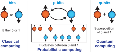Fig. 1: bit, p-bit, and qubit : Each column shows a schematic representation of the basic computational units of classical computing (left), probabilistic computing (middle), and quantum computing (right). These are, respectively, the bit, the p-bit, and the qubit. <details> <summary>Image 1 Details</summary>  ### Visual Description ## Diagram: Comparison of Bits, P-bits, and Qubits ### Overview The image presents a comparative diagram illustrating the concepts of bits, p-bits, and qubits, representing classical, probabilistic, and quantum computing, respectively. Each type of bit is visually represented with a diagram of a sphere with an arrow. ### Components/Axes * **Title:** The diagram is divided into three sections, each labeled with a different type of bit: "bits", "p-bits", and "qubits". The labels are in blue. * **Bits (Classical Computing):** * Represents classical computing. * Shows two possible states: a red sphere with an upward arrow and a blue sphere with a downward arrow. * Text: "or" is placed between the two states. * Text: "Either 0 or 1" is below the states. * Text: "Classical computing" is below the "Either 0 or 1" text. * **P-bits (Probabilistic Computing):** * Represents probabilistic computing. * Shows a red sphere with an upward arrow and a blue sphere with a downward arrow, connected by a curved double-headed arrow, indicating fluctuation between the two states. * Below the p-bits is a rectangle containing multiple red spheres with upward arrows and blue spheres with downward arrows. The red spheres are clustered at the top of the rectangle, and the blue spheres are clustered at the bottom. * Text: "Fluctuates between 0 and 1" is below the rectangle. * Text: "Probabilistic computing" is below the "Fluctuates between 0 and 1" text. * **Qubits (Quantum Computing):** * Represents quantum computing. * Shows a red sphere with an upward arrow and a blue sphere with a downward arrow, connected by a "+" sign, indicating superposition. * Text: "Superposition of 0 and 1" is below the states. * Text: "Quantum computing" is below the "Superposition of 0 and 1" text. ### Detailed Analysis or ### Content Details * **Bits:** A bit can be either 0 or 1. The diagram shows a red sphere with an upward arrow representing one state and a blue sphere with a downward arrow representing the other state. * **P-bits:** A p-bit fluctuates between 0 and 1. The diagram shows a red sphere with an upward arrow and a blue sphere with a downward arrow, connected by a curved double-headed arrow. The rectangle below shows a collection of p-bits, with a tendency for red spheres (0) to be at the top and blue spheres (1) to be at the bottom. * **Qubits:** A qubit can be in a superposition of 0 and 1. The diagram shows a red sphere with an upward arrow and a blue sphere with a downward arrow, connected by a "+" sign. ### Key Observations * The diagram visually distinguishes between classical, probabilistic, and quantum computing by illustrating the states and behaviors of bits, p-bits, and qubits. * The use of color (red and blue) consistently represents the two possible states (0 and 1) across all three types of bits. * The arrows indicate the direction of spin or state. ### Interpretation The diagram effectively illustrates the fundamental differences between classical, probabilistic, and quantum computing. Classical bits have definite states (0 or 1), p-bits fluctuate between these states, and qubits can exist in a superposition of both states simultaneously. The visual representation of these concepts helps to understand the underlying principles of each computing paradigm. The clustering of red and blue spheres in the p-bits section suggests a probabilistic distribution, where the bit is more likely to be in one state than the other at any given time. The "+" sign in the qubits section emphasizes the superposition principle, a key feature of quantum computing. </details> entirely new approaches using spintronic and magnetoelectric phenomena to build energy-efficient switches [6, 7]. A complementary approach to extending Moore's Law is to augment the existing CMOS ecosystem with emerging, nonsilicon nanotechnologies [8, 9]. One way to achieve this goal is through heterogeneous CMOS + X architectures where X stands for a CMOS-compatible nanotechnology. For example, X can be magnetic, ferroelectric, memristive or photonic systems. We also discuss an example of this complementary approach, the combination of CMOS with magnetic memory technology, purposefully modified to build probabilistic computers. ## II. FULL-STACK VIEW AND ORGANIZATION Research on probabilistic computing with p-bits originated at the device and physics level, first with stable nanomagnets [10], followed by low barrier nanomagnets [11, 12]. In [12], the p-bit was formally defined as a binary stochastic neuron realized in hardware. In both approaches with stable and unstable nanomagnets, the basic idea is to exploit the natural mapping between the intrinsically noisy physics of nanomagnets to the mathematics of general probabilistic algorithms (e.g., Monte Carlo, Markov Chain Monte Carlo). Such a notion of natural computing where physics is matched to computation was clearly laid out by Feynman in his celebrated Simulating Physics with Computers talk [13]. Subsequent work on p-bits defined it as an abstraction between bits and qubits (FIG. 1) with the possibility of different physical implementations. In addition to searching for energy-efficient realizations of single devices, p-bit research has extended to finding efficient architectures (through massive parallelization, sparsification [14] and pipelining [15]) along with the identification of promising application domains. 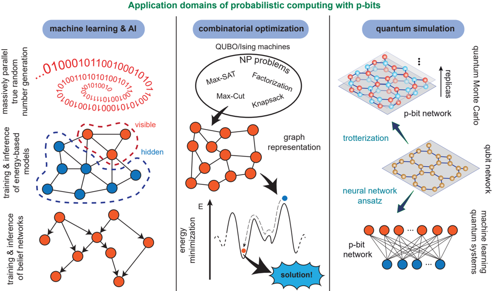This full-stack research program covering hardware, architecture, algorithms, and applications is similar to the related field of quantum computation where a large degree of interdisciplinary expertise Fig. 2: Applications of probabilistic computing : Potential applications of p-bits are illustrated. The list broadly includes problems in combinatorial optimization, probabilistic machine learning, and quantum simulation. <details> <summary>Image 2 Details</summary>  ### Visual Description ## Application Domains Diagram: Probabilistic Computing with p-bits ### Overview The image is a diagram illustrating the application domains of probabilistic computing using p-bits. It is divided into three main sections: machine learning & AI, combinatorial optimization, and quantum simulation. Each section depicts a specific application area with corresponding diagrams and labels. ### Components/Axes * **Title:** Application domains of probabilistic computing with p-bits * **Sections (Left to Right):** * Machine Learning & AI * Combinatorial Optimization * Quantum Simulation * **Labels within Sections:** * **Machine Learning & AI:** * massively parallel true random number generation * training & inference of energy-based models * training & inference of belief networks * visible (red dashed line) * hidden (blue dashed line) * **Combinatorial Optimization:** * QUBO/Ising machines * NP problems * Max-SAT * Max-Cut * Factorization * Knapsack * graph representation * energy minimization (E) * solution! * **Quantum Simulation:** * replicas * p-bit network * trotterization * qubit network * neural network ansatz * p-bit network * machine learning quantum systems * quantum Monte Carlo ### Detailed Analysis **Machine Learning & AI:** * **Massively Parallel True Random Number Generation:** A sequence of 0s and 1s arranged in a circular pattern. * **Training & Inference of Energy-Based Models:** A network of interconnected nodes, some colored red (inside a dashed red "visible" region) and some blue (inside a dashed blue "hidden" region). * **Training & Inference of Belief Networks:** A directed graph with nodes and arrows indicating relationships. **Combinatorial Optimization:** * **QUBO/Ising Machines:** A collection of NP problems (Max-SAT, Max-Cut, Factorization, Knapsack) contained within an oval shape. * **Graph Representation:** A network of interconnected nodes. * **Energy Minimization:** A graph showing energy (E) on the vertical axis. A solid line represents the energy landscape, and a dashed line represents a possible path to a solution. A red dot indicates a local minimum, and a blue dot indicates the global minimum ("solution!"). **Quantum Simulation:** * **Replicas:** Two layers of interconnected nodes, one above the other, representing replicas of a p-bit network. * **Trotterization:** An arrow pointing from the p-bit network to a qubit network. * **Neural Network Ansatz:** An arrow pointing from the qubit network to a p-bit network. * **Machine Learning Quantum Systems:** A p-bit network connected to quantum systems. ### Key Observations * The diagram illustrates three distinct application domains for probabilistic computing with p-bits. * Each section uses different visual representations to depict the specific application. * The "visible" and "hidden" labels in the Machine Learning & AI section suggest a distinction between observable and latent variables. * The energy minimization graph in the Combinatorial Optimization section highlights the process of finding optimal solutions. * The Quantum Simulation section shows the relationship between p-bit networks, qubit networks, and quantum systems. ### Interpretation The diagram provides a high-level overview of how probabilistic computing with p-bits can be applied to various fields. It demonstrates the versatility of p-bits in addressing problems in machine learning, combinatorial optimization, and quantum simulation. The diagram suggests that p-bits can be used for tasks such as generating random numbers, training energy-based models, solving NP problems, and simulating quantum systems. The connections between different types of networks (p-bit, qubit) in the quantum simulation section indicate a potential for hybrid computing approaches. The diagram emphasizes the importance of energy minimization in finding solutions to complex problems. </details> is required to move the field forward (see the related reviews Ref. [16, 17]). The purpose of this paper is to serve as a consolidated summary of recent developments with new results in hardware, architectures, and algorithms. We provide concrete and previously unpublished examples of machine learning and AI, combinatorial optimization, and quantum simulation with p-bits (FIG. 2). ## III. FUNDAMENTALS OF P-COMPUTING A large family of problems (FIG. 2) can be encoded to coupled p-bits evolving according to the following equations [12]: $$\begin{array} { r l r } { m _ { i } } & = } & { s i g n \left [ t a n h ( \beta I _ { i } ) - r _ { [ - 1 , + 1 ] } \right ] } & { ( 1 ) } & { d e s c r i j i n g } \end{array}$$ <!-- formula-not-decoded --> where m i is defined as a bipolar variable ( m ∈ {-1 , +1 } ), r is a uniform random number drawn from the interval [ -1 , 1] , [ W ] is the coupling matrix between the p-bits, β is the inverse temperature and { h } is the bias vector. In physical implementations, it is often more convenient to represent p-bits as binary variables, s i ∈ { 0 , 1 } . A straightforward conversion of Eq. (1) and Eq. (2) is possible using the standard transformation, m → 2 s -1 [18]. As stated, Eq. (1) and Eq. (2) do not place any restrictions on the [ W ] , which may be a symmetric or asymmetric matrix. If an update order of p-bits is specified, these equations take the coupled p-bit system to a well-defined steady-state distribution defined by the eigenvector (with eigenvalue +1 ) of the corresponding Markov matrix [12]. Indeed, in case of Bayesian (belief) networks defined by a directed graph, updating the p-bits from parent nodes to child nodes takes the system to a steady-state distribution corresponding to that obtained from the Bayes' Theorem [19]. If the [ W ] matrix is symmetric, one can define an energy, E , whose negated partial derivative with respect to p-bit m i gives rise to Eq. (2): <!-- formula-not-decoded --> In this case, the steady-state distribution of the network is described by [20]: <!-- formula-not-decoded --> also known as the Boltzmann Law. As such, iterating a network of p-bits described by Eq. (1) and Eq. (2) eventually approximates the Boltzmann distribution which can be useful for probabilistic sampling and optimization. The approximate sampling avoids the intractable problem of exactly calculating Z . Remarkably, for such undirected networks, the steady-state distribution is invariant with respect to the update order of pbits, as long as connected p-bits are not updated at the same time (more on this later). This feature is highly reminiscent of natural systems where asynchronous dynamics make parallel updates highly unlikely and the update order does not change the equilibrium distribution. Indeed, this gives the hardware implementation of asynchronous networks of p-bits massive parallelism and flexibility in design. The energy functional defined by Eq. (3) is often the starting point of discussions in the related field of Ising Machines [21-43] with different implementations (see, Ref. [44] for a comprehensive review). In the case of p-bits, however, we view Eq. (1) and Eq. (2) more fundamental than Eq. (3) because the former can also be used to approximate hard inference on directed networks while the latter always relies on undirected networks. Compared to undirected networks using Ising Machines, work on directed neural networks for Bayesian inference has been relatively scarce, although there are exciting developments [19, 45-50]. Finally, the form of Eq. (3) restricts the type of interactions between p-bits to a linear one since the energy is quadratic. Even though higher-order interactions ( k -local) between pbits are possible [18] (also discussed in the context of Ising machines [51, 52]), such higher-order interactions can always be constructed by combining a standard probabilistic gate set at the cost of extra p-bits. In our view, in the case of electronic implementation with scalable p-bits, trading an increased number of p-bits for simplified interconnect complexity is almost always favorable. That being said, algorithmic advantages and the better representative capabilities of higherorder interactions are actively being explored [51, 53]. ## IV. HARDWARE: PHYSICAL IMPLEMENTATION OF P-BITS A. p-bit The p-bit defined in Eq. (1) describes a tunable and discrete random number generator. Its physical implementation includes a broad range of options from noisy materials to analog and digital CMOS (FIG. 3). The digital CMOS implementations of p-bits often consist of a pseudorandom number generator (PRNG) ( r ), a lookup table for the activation function (tanh), and a threshold to generate a one-bit output. A digital input with a specified fixed point precision (e.g., 10 bits with 1 sign, 6 integers and 3 fractional) provides tunability through the activation function. Digital p-bits have been very useful in prototyping probabilistic computers up to tens of thousands of p-bits [54, 55, 14]. They also serve a useful purpose to illustrate why analog or mixed-signal implementations of pbits with nanodevices are necessary. Even using some of the most advanced field programmable gate arrays (FPGA), the footprint of a digital p-bit is very large: Synthesizing such digital p-bits with pseudo-random number generators (PRNGs) of varying quality of randomness results in tens of thousands of individual transistors. In single FPGAs that do not use timedivision multiplexing of p-bits or off-chip memory, only about 10,000 to 20,000 p-bits with 100,000 weights (sparse graphs with degree 5 to 10) fit, even within high-end devices [14]. On the other hand, using nanodevices such as CMOScompatible stochastic magnetic tunnel junctions (sMTJ), millions of p-bits can be accommodated in single cores due to the scalability achieved by the MRAM technology, exceeding 1Gbit MRAM chips [56, 57]. However, before the stable MTJs can be controllably made stochastic, challenges at the material and device level must be addressed [58, 59] with careful magnet design [60-62]. Different flavors of magnetic p-bits exist [63-66], for a recent review, see Ref. [67]. 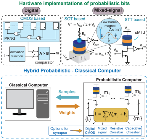Unlike synchronous or trial-based stochasticity (e.g., [68]) that re- Fig. 3: Different hardware options for building a probabilistic computer : (Top) Various magnetic implementations of a p-bit. These include both digital (CMOS) and mixed-signal implementations (based on, for example, stochastic magnetic tunnel junction with low barrier magnets). (Bottom) A hybrid of classical and probabilistic computing schemes is shown where the classical computer generates weights and programs the probabilistic computer. The probabilistic computer then generates samples accordingly with high throughput and sends them back to the classical computer for further processing. Like the building blocks of p-bits, the synapse of the probabilistic computer can be designed in several ways, including digital, analog, and a mix of both techniques. <details> <summary>Image 3 Details</summary>  ### Visual Description ## Hardware Implementations of Probabilistic Bits and Hybrid Computer Architecture ### Overview The image presents a diagram illustrating hardware implementations of probabilistic bits using digital and mixed-signal approaches, along with a hybrid probabilistic-classical computer architecture. It details CMOS-based, SOT-based, and STT-based implementations, and shows how a classical computer can interface with a probabilistic computer. ### Components/Axes **Header:** * Title: "Hardware implementations of probabilistic bits" * Categories: "Digital" and "Mixed-signal" are distinguished by rounded boxes. **Digital Implementation (Left):** * CMOS based: * PRNG (Pseudo-Random Number Generator): A series of flip-flops connected with XOR gates. * Activation function: A block labeled "activation function" takes an input "I". * Comparator: A comparator block labeled "A > B" with inputs from the activation function and PRNG, and output "m". **Mixed-Signal Implementations (Right):** * SOT based: * Equation: V+ = VDD / 2 + VR * Resistor: Labeled R0. * MTJ (Magnetic Tunnel Junction): A cylinder with alternating blue and orange layers. * Input: VIN * Output: VOUT * Current: Is * Equation: V- = VDD / 2 * Low barrier magnet: A circular inset showing a potential energy landscape with two minima, labeled Eb and Δ ≈ 0 kT, and angle θ. * STT based: * sMTJ (spintransfer-torque Magnetic Tunnel Junction): A cylinder with alternating blue and orange layers. * Voltage: VDD * Input: VIN * Output: VOUT **Hybrid Probabilistic - Classical Computer (Bottom):** * Title: "Hybrid Probabilistic - Classical Computer" * Classical Computer: A representation of a computer monitor and tower. * Probabilistic Computer: * Multiple MTJ-based probabilistic bit implementations (m1 to mN). * Equation: Ii = Σj Wijmj + hi * Inputs: {li} * Outputs: {mi} * Arrows: * "Samples" (blue arrow) flows from the Probabilistic Computer to the Classical Computer. * "Weights" (orange arrow) flows from the Classical Computer to the Probabilistic Computer. * Options for synapse: An arrow pointing to a table with the following categories: Digital CMOS, Mixed signal, Resistive Crossbar, Capacitive Crossbar. ### Detailed Analysis or ### Content Details **Digital Implementation:** * The CMOS-based implementation uses a PRNG to generate random bits. * An activation function processes an input signal "I". * A comparator compares the output of the activation function with the PRNG output to generate a probabilistic bit "m". **Mixed-Signal Implementations:** * The SOT-based implementation uses a Spin-Orbit Torque (SOT) device. The voltage V+ is defined as VDD/2 + VR. * The STT-based implementation uses a Spin-Transfer Torque (STT) device. * Both SOT and STT implementations use MTJs to represent probabilistic bits. **Hybrid Computer Architecture:** * The Classical Computer and Probabilistic Computer exchange information. * The Classical Computer sends "Weights" to the Probabilistic Computer. * The Probabilistic Computer sends "Samples" to the Classical Computer. * The probabilistic computer calculates Ii as the sum of Wijmj + hi, where Wij are weights, mj are probabilistic bits, and hi are biases. * Synapse options include Digital CMOS, Mixed signal, Resistive Crossbar, and Capacitive Crossbar. ### Key Observations * The diagram illustrates different hardware approaches to implement probabilistic bits. * The hybrid architecture combines classical and probabilistic computing paradigms. * The mixed-signal implementations leverage spintronic devices (SOT and STT) and MTJs. ### Interpretation The diagram presents a vision for integrating probabilistic computing with classical computing. The different hardware implementations of probabilistic bits (CMOS, SOT, STT) offer various trade-offs in terms of speed, power consumption, and area. The hybrid architecture allows leveraging the strengths of both classical and probabilistic computing, potentially enabling new applications in areas such as machine learning, optimization, and cryptography. The "Options for synapse" suggest different ways to implement the connections between probabilistic bits, each with its own advantages and disadvantages. </details> quires continuous resetting, the temporal noise of low-barrier nanomagnets makes them ideally suited to build autonomous, physics-inspired probabilistic computers, providing a constant stream of tunably random bits [69]. Following earlier theoretical predictions [70-72], recent breakthroughs in low-barrier magnets have shown great promise, using stochastic MTJs with in-plane anisotropy where fluctuations can be of the order of nanoseconds [73-75]. Such near-zero barrier nanomagnets should be more tolerant to device variations because when the energy-barrier ∆ is low, the usual exponential dependence of fluctuations is much less pronounced. These stochastic MTJs may be used in electrical circuits with a few additional transistors (FIG. 3) to build hardware p-bits. Two flavors of stochastic MTJ-based p-bits were proposed in Ref. [12] (SOT-based) and in Ref. [70] (STT-based). Both of these p-bits have now been experimentally demonstrated in Refs. [18, 76, 77] (STT) and in Ref. [78] (SOT). While many other implementations of p-bits are possible, from molecular nanomagnets [79] to diffusive memristors [80], RRAM [81], perovskite nickelates [82] and others, two additional advantages of the MRAM-based p-bits are the proven manufacturability (up to billion bit densities) and the amplification of room temperature noise. Even with the thermal energy of kT in the environment, magnetic switching causes large resistance fluctuations in MTJs, creating hundreds of millivolts of change in resistive dividers [70]. Typical noise on resistors (or memristors) is limited by the √ kT/C limit which is far lower (millivolts) even at extremely low capacitances ( C ). 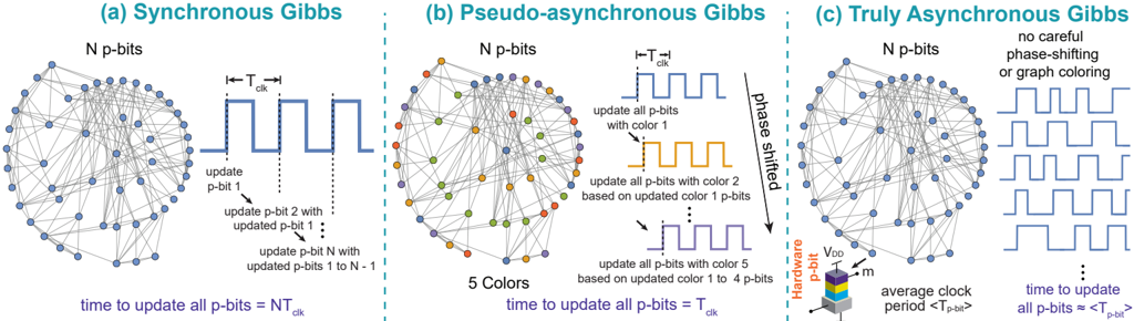This feature of stochastic MTJs ensures Fig. 4: Architectures of p-computer : (a) Synchronous Gibbs: all p-bits are updated sequentially. N p-bits need N clock cycles ( NT clk ) to perform a complete sweep, T clk being the clock period. (b) Pseudo-asynchronous Gibbs: a sparse network can be colored into a few disjoint blocks where connected p-bits are assigned a different color. Phase-shifted clocks update the color blocks one after the other. N p-bits need ≈ 1 clock cycle T clk to perform a complete sweep, reducing O( N ) complexity of a sweep to O( 1 ), where we assume the number of colors c N . (c) Truly Asynchronous Gibbs: a hardware p-bit (e.g., a stochastic MTJ-based p-bit) provides an asynchronous and random clock with period 〈 T p-bit 〉 . N p-bits need approximately 1 clock to perform a complete sweep, as long as synapse time is less than the clock on average. No graph coloring or engineered phase shifting is required. <details> <summary>Image 4 Details</summary>  ### Visual Description ## Diagram: Synchronous, Pseudo-asynchronous, and Truly Asynchronous Gibbs ### Overview The image presents three diagrams illustrating different approaches to Gibbs sampling: Synchronous, Pseudo-asynchronous, and Truly Asynchronous. Each diagram includes a network of interconnected nodes representing 'N p-bits', along with a timing diagram showing how these bits are updated. ### Components/Axes * **Titles:** * (a) Synchronous Gibbs * (b) Pseudo-asynchronous Gibbs * (c) Truly Asynchronous Gibbs * **Network Diagrams:** Each diagram features a network of nodes (representing p-bits) connected by lines. * **Timing Diagrams:** Each diagram includes a timing diagram illustrating the update sequence of the p-bits. * **Labels:** * N p-bits (present in all three diagrams) * Tclk (clock period) * VDD * m * Hardware p-bit * **Textual Annotations:** * Diagram (a): "update p-bit 1", "update p-bit 2 with updated p-bit 1", "update p-bit N with updated p-bits 1 to N-1", "time to update all p-bits = NTclk" * Diagram (b): "5 Colors", "update all p-bits with color 1", "update all p-bits with color 2 based on updated color 1 p-bits", "update all p-bits with color 5 based on updated color 1 to 4 p-bits", "time to update all p-bits = Tclk", "phase shifted" * Diagram (c): "no careful phase-shifting or graph coloring", "average clock period <Tp-bit>", "time to update all p-bits ≈ <Tp-bit>" ### Detailed Analysis **Diagram (a): Synchronous Gibbs** * **Network:** A network of approximately 40 nodes (p-bits), all colored blue, connected by gray lines. * **Timing Diagram:** A single clock signal with period Tclk. All p-bits are updated sequentially within each clock cycle. The update sequence is explicitly described: p-bit 1 is updated first, then p-bit 2 based on the updated p-bit 1, and so on until p-bit N is updated based on the updated p-bits 1 to N-1. * **Time to Update:** The total time to update all p-bits is NTclk, where N is the number of p-bits. **Diagram (b): Pseudo-asynchronous Gibbs** * **Network:** A network of approximately 40 nodes (p-bits), colored with 5 different colors: blue, orange, green, yellow, and purple. The nodes are connected by gray lines. * **Timing Diagram:** Three phase-shifted clock signals are shown. The first clock signal (blue) updates all p-bits with color 1. The second clock signal (orange) updates all p-bits with color 2 based on the updated color 1 p-bits. The last clock signal (purple) updates all p-bits with color 5 based on the updated color 1 to 4 p-bits. * **Time to Update:** The total time to update all p-bits is Tclk. **Diagram (c): Truly Asynchronous Gibbs** * **Network:** A network of approximately 40 nodes (p-bits), all colored blue, connected by gray lines. * **Timing Diagram:** Multiple clock signals are shown, with no careful phase-shifting or graph coloring. * **Hardware p-bit:** A diagram of a hardware p-bit is shown, with labels VDD and m. The p-bit is composed of stacked layers of blue, yellow, and purple. * **Time to Update:** The average clock period is less than Tp-bit, and the time to update all p-bits is approximately equal to Tp-bit. ### Key Observations * **Synchronous Gibbs:** Updates all p-bits sequentially within each clock cycle, resulting in a longer update time. * **Pseudo-asynchronous Gibbs:** Uses color-based updating with phase-shifted clock signals, reducing the update time. * **Truly Asynchronous Gibbs:** Updates p-bits asynchronously without careful phase-shifting or graph coloring, achieving the shortest update time. ### Interpretation The diagrams illustrate the trade-offs between different Gibbs sampling approaches in terms of update time and complexity. Synchronous Gibbs is the simplest but slowest, while Truly Asynchronous Gibbs is the fastest but requires more complex hardware and control. Pseudo-asynchronous Gibbs offers a compromise between speed and complexity by using color-based updating with phase-shifted clock signals. The choice of which approach to use depends on the specific application and the desired balance between speed, hardware complexity, and control overhead. </details> that they do not require explicit amplifiers [83] at each p-bit, which can become prohibitively expensive in terms of area and power consumption. Estimates of sMTJs-based p-bits suggest they can create a random bit using 2 fJ per operation [18]. Recently, a CMOS-compatible single photon avalanche diodebased implementation of p-bits showed similar, amplifierfree operation [84] and the search for the most scalable, energy-efficient hardware p-bit using alternative phenomena continues. ## B. Synapse The second central part of the p-computer architecture is the synapse, denoted by Eq. (2). Much like the hardware p-bit, there are several different implementations of synapses ranging from digital CMOS, analog/mixed-signal CMOS as well as resistive [85] or capacitors crossbars [86, 87]. The synaptic equation looks like the traditional matrix-vector product (MVP) commonly used in ML models today, however, there is a crucial difference: thanks to the discrete p-bit output (0 or 1), the MVP operation is simply an addition over the active neighbors of a given p-bit. This makes the synaptic operation simpler than continuous multiplication and significantly simplifies digital synapses. In analog implementations, the use of in-memory computing techniques through charge accumulation could be useful with the added simplification of digital outputs of p-bits [88, 89]. It is important to note how the p-bit and the neuron for eventually integrated p-bit applications can be mixed and matched, as an example of creatively combining these pieces, see the FPGA-stochastic MTJ combination reported in Ref. [77]. The best combination of scalable p-bits and synapses may lead to energy-efficient and large scale p-computers. At this time, various possibilities exist with different technological maturity. ## V. ARCHITECTURE CONSIDERATIONS ## A. Gibbs sampling with p-bits The dynamical evolution of Eqs. (1-2) relies on an iterated updating scheme where each p-bit is updated one after the other based on a predefined (or random) update order. This iterative scheme is called Gibbs sampling [90, 91]. Virtually all applications discussed in Fig. 2 benefit from accelerating Gibbs sampling, attesting to its generality. In a standard implementation of Gibbs sampling in a synchronous system, p-bits will be updated one by one at every clock cycle as shown in FIG. 4a. It is crucial to ensure that the effective input each p-bit receives through Eq. (2) is computed before the p-bit updates. As such, the T clk has to be longer than the time it takes to compute Eq. (2). In this setting, a graph with N p-bits will require N clock cycles ( NT clk ) to perform a complete sweep where T clk is the clock period. This requirement makes Gibbs sampling a fundamentally serial and slow process. Amuch more effective approach is possible by the following observation: even though updates between connected p-bits need to be sequential, if two p-bits are not directly connected, updating one of them does not directly change the input of the other through Eq. (2). Such p-bits can be updated in parallel without any approximation. Indeed, one motivation of designing restricted Boltzmann machines (RBMs, see Ref. [92]) over unrestricted BMs is to exploit this parallelism: RBMs consist of separate layers (bipartite) that can be updated in parallel. However, this idea can be taken further. If the underlying graph is sparse , it is often easy to split it into disconnected chunks by coloring the graph using a few colors. Even though finding the minimum number of colors is an NP-hard problem [93], heuristic coloring algorithms (such as Dsatur [94]) with polynomial complexity can color the graph very quickly, without necessarily finding a minimum. In this context obtaining the minimum coloring is not critical and sparse graphs typically require a few colors. Such an approach was taken on sparse graphs (with no regular structure) to design a massively parallel implementation of Gibbs sampling in Ref. [14] (FIG. 4b). Connected p-bits are assigned a different color and unconnected p-bits are assigned the same color. Equally phase-shifted and samefrequency clocks update the p-bits in each color block one by one. In this approach, a graph with N p-bits requires only 1 clock cycle ( T clk ) to perform a complete sweep, reducing O( N ) complexity for a full sweep to O (1) , assuming the number of colors is much less than N . Therefore, the key advantage of this approach is that the p-computer becomes faster with larger graphs since probabilistic 'flips per second', a key metric measured by TPU and GPU implementations [95, 96] linearly increases with the number of p-bits. It is important to note that these TPU and GPU implementations also solve Ising problems in sparse graphs, however, their graph degrees are usually restricted to 4 or 6, unlike more irregular and higher degree graphs implemented in Ref. [14]. We term this graph-colored architecture the pseudoasynchronous Gibbs because while it is technically synchronized to out-of-phase clocks, it embodies elements of the truly asynchronous architecture we discuss next. While graph coloring algorithmically increases sampling rates by a factor of N , it still requires a careful design of out-of-phase clocks. A much more radical approach is to design a truly asynchronous Gibbs sampler as shown in FIG. 4c. Here, the idea is to have hardware building blocks with naturally asynchronous dynamics, such as a stochastic magnetic tunnel junction-based p-bit. In such a p-bit, there exists a natural 'clock', 〈 T p-bit 〉 , defined by the average lifetime of a Poisson process [97]. As long as 〈 T p-bit 〉 is not faster than the average synapse time ( t synapse ) to calculate Eq. (2), the network still updates N spins in a single 〈 T p-bit 〉 timescale. This is because the probability of simultaneous updates is extremely low in a Poisson process and further reduced in highly sparse graphs. In fact, preliminary experiments implementing such truly asynchronous p-bits with ring-oscillator activated clocks show that despite making occasional parallel updates, the asynchronous p-computer performs similarly compared to the pseudo-asynchronous system where incorrect updates are avoided with careful phase-shifting [98]. The main appeal of the truly asynchronous Gibbs sampling is the lack of any graph coloring and phase-shift engineering while retaining the same massive parallelism as N p-bits requires approximately a single 〈 T p-bit 〉 to complete a sweep. Given that the FPGAbased p-computers already provide about a 10X improvement in sampling throughput to optimized TPU and GPUs [14], such asynchronous systems are promising in terms of scalability. Stochastic MTJ-based p-bits should be able to reach high densities on a single chip. Around 20 W of projected power consumption can be reached considering 20 µ Wp-bit/synapse combinations at 1M p-bit density [54, 99, 60]. The ultimate scalability of magnetic p-bits is a significant advantage over alternative approaches based on electronic or photonic devices. ## B. Sparsification Both the pseudo-asynchronous and the truly asynchronous parallelism require sparse graphs to work well. The first problem is the number of colors: if the graph is dense, it requires a lot of colors, making the architecture very similar to the standard serial Gibbs sampling. The second problem with a dense graph is the synapse time, t synapse . If many p-bits have a lot of neighbors, the synapse unit needs to compute a large sum before the next update. 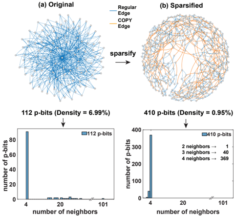If the time between two consecutive updates is 〈 T p-bit 〉 , it requires Fig. 5: (a) Original graph of a 3SAT instance uf20-01.cnf [100] having 112 p-bits and a graph density of 6.99%. (Graph density, ρ = 2 | E | / ( | V | 2 -| V | ) where | E | = the number of edges and | V | = the number of vertices in the graph). Some of the p-bits have many local neighbors up to 101 neighbors as shown in the histogram which slows down the synapse and the p-bits need to update slowly. (b) Sparsified graph of the same instance having 410 pbits. COPY gates are inserted between each pair of copies of the same p-bits (COPY edges are highlighted in orange). The graph has a density of 0 . 95% and the maximum number of neighbors is limited to 4 . The synapse operations are now faster and hence the p-bits can be updated faster. Even though the example shown here starts from a low-density graph, the sparsification algorithm we give is general and applicable to any graph. <details> <summary>Image 5 Details</summary>  ### Visual Description ## Network Sparsification and Degree Distribution ### Overview The image presents a comparison between an original network and its sparsified version, along with their respective degree distributions. The image is divided into two columns, (a) Original and (b) Sparsified. Each column contains a network diagram and a histogram showing the number of p-bits versus the number of neighbors. The sparsification process reduces the density of the network, which is reflected in the change in the degree distribution. ### Components/Axes **Top Row: Network Diagrams** * **(a) Original:** A dense network diagram with nodes connected by "Regular Edge" (blue lines). * **(b) Sparsified:** A less dense network diagram with nodes connected by "Regular Edge" (blue lines) and "COPY Edge" (orange lines). * **Legend (Top-Right):** * Regular Edge: Blue line * COPY Edge: Orange line * **Process Indicator:** An arrow labeled "sparsify" points from the original network to the sparsified network. **Bottom Row: Histograms (Degree Distributions)** * **X-axis (both histograms):** "number of neighbors" with tick marks at 4, 20, and 101. A break in the x-axis indicates a discontinuity in the scale. * **Y-axis (both histograms):** "number of p-bits" ranging from 0 to 80 for the original network and 0 to 400 for the sparsified network. * **Histogram Bars:** Blue bars representing the frequency of each number of neighbors. * **Titles above Histograms:** * Left: "112 p-bits (Density = 6.99%)" * Right: "410 p-bits (Density = 0.95%)" * **Legends within Histograms:** * Left: "112 p-bits" * Right: "410 p-bits" * **Additional Text (Right Histogram):** * 2 neighbors → 1 * 3 neighbors → 40 * 4 neighbors → 369 ### Detailed Analysis or ### Content Details **Network Diagrams:** * **(a) Original:** The network appears highly connected, with many blue edges linking the nodes. * **(b) Sparsified:** The network has fewer blue edges and the introduction of orange edges. The overall connectivity is reduced. **Histograms:** * **(a) Original:** * The histogram is heavily skewed towards a small number of neighbors. * The bar at 4 neighbors reaches approximately 80 p-bits. * The bars for higher numbers of neighbors are very small, close to zero. * **(b) Sparsified:** * The histogram is also skewed towards a small number of neighbors, but the distribution is different from the original. * The bar at 4 neighbors reaches approximately 370 p-bits. * The text indicates specific values: 2 neighbors (1 p-bit), 3 neighbors (40 p-bits), and 4 neighbors (369 p-bits). ### Key Observations * The sparsification process significantly reduces the density of the network (from 6.99% to 0.95%). * The number of p-bits increases from 112 to 410 after sparsification. * The degree distribution shifts after sparsification, with a higher concentration of nodes having a small number of neighbors (specifically 4 neighbors). ### Interpretation The image illustrates the effect of sparsification on a network and its degree distribution. Sparsification, while reducing the overall density of connections, can lead to a redistribution of node degrees. The increase in p-bits after sparsification suggests that the process involves adding new nodes or connections, even as it removes others. The degree distributions show that both the original and sparsified networks are dominated by nodes with a small number of neighbors, but the sparsified network has a much higher concentration of nodes with 4 neighbors. This could indicate that the sparsification algorithm preferentially creates or preserves connections that result in nodes having a degree of 4. The "COPY Edge" likely represents edges that were created during the sparsification process, potentially duplicating or re-wiring existing connections. </details> t synapse 〈 T p-bit 〉 to avoid information loss and reach the correct steady-state distribution [101, 54]. However, if the graph is sparse, each p-bit has fewer connections and the updates can be faster without any dropped messages. Any graph can be sparsified using the technique proposed in [14], similar in spirit to the minor-graph embedding (MGE) approach pioneered by D-Wave [102], even though the objective here is to not find an embedding but to sparsify an existing graph. The key idea is to split p-bits into different copies, using ferromagnetic COPY gates. These p-bits distribute the original connections among them, resulting in identical copies with fewer connections. An important point is that the ground-state of the original graph remains unchanged [14], so the method does not involve approximations, unlike other sparsification techniques, for example, based on low-rank approximations [103]. FIG. 5a shows an example of this process where the original graph of a satisfiability (3SAT) instance has been sparsified as shown in FIG. 5b. Irrespective of the input graph size, a sparsified graph has fewer connections locally and thus the neurons hardly ever need to be slowed down. One disadvantage of this technique is the increased number of p-bits, however, the reduced synapse complexity and the possibility of massive parallelization outweigh the costs incurred by additional p-bits, which we consider to be cheap in scaled, nanodevice-based implementations. + <details> <summary>Image 6 Details</summary>  ### Visual Description ## Problem Formulations: Max-SAT, Number Partitioning, and Knapsack ### Overview The image presents three different problem formulations: Max-SAT, Number Partitioning, and Knapsack. Each problem is described using a mathematical formulation, an invertible logic formulation, and an Ising model formulation. The image provides equations, logic diagrams, and heatmaps to represent each problem. ### Components/Axes **General Layout:** The image is divided into three vertical sections, one for each problem: Max-SAT (left), Number Partitioning (center), and Knapsack (right). Each section is further divided into three horizontal sections: Mathematical formulation (top), Invertible logic formulation (middle), and Ising model formulation (bottom). **Max-SAT (Left Section):** * **Mathematical formulation:** * Objective: maximize ∑(from c=1 to Nc) vc * Constraint: vc = yc1 ∨ yc2 ∨ ... ∨ ycn * Domain: vc ∈ {0, 1}, yx ∈ {0, 1} * **Invertible logic formulation:** * Logic gates: Probabilistic OR (red), Probabilistic AND (orange) * Inputs: y1 (green), y2 (cyan), y3 (magenta), y4 (brown) * Outputs: c1, c2, c3, and a final AND gate outputting 1. * Text: "Clamp missing 1 clauses to 1", "Clamp all clauses to 1" * **Ising model formulation:** * Heatmap: A square matrix with values ranging from -2 (red) to +2 (blue). * Colorbar: Ranges from -2 (red) to +2 (blue), with intermediate values of -1, 0, and +1. **Number Partitioning (Center Section):** * **Mathematical formulation:** * Objective: minimize |∑(from i=1 to N) sini| * Constraint: si ∈ {-1, +1} * **Invertible logic formulation:** * Components: 2-bit adders (light blue), Probabilistic XOR (purple) * Inputs: n1, s1, n2, s2 * Text: "2's complement", "Sign choice", "Clamp sum of sets to 0" * **Ising model formulation:** * Heatmap: A square matrix with values ranging from -2 (red) to +2 (blue). * Colorbar: Ranges from -2 (red) to +2 (blue), with intermediate values of -1, 0, and +1. **Knapsack (Right Section):** * **Mathematical formulation:** * Objective: maximize ∑(from i=1 to N) vixi * Constraint: ∑(from i=1 to N) wixi ≤ W * Domain: vi ≥ 0, wi ≥ 0, xi ∈ {0, 1} * **Invertible logic formulation:** * Components: 2-bit adders (light blue), Probabilistic AND (orange) * Inputs: v1, w1, x1, v2, w2, x2 * Text: "2's complement", "Clamp sum of values to MAX", "Clamp sum of weights to <W", "-W", "MAX" * **Ising model formulation:** * Heatmap: A square matrix with values ranging from -2 (red) to +2 (blue). * Colorbar: Ranges from -2 (red) to +2 (blue), with intermediate values of -1, 0, and +1. **Legend (Bottom):** Located at the bottom center of the image. * Probabilistic OR: Red gate symbol * Probabilistic AND: Orange gate symbol * Probabilistic XOR: Purple gate symbol * Probabilistic n-bit Adder: Light blue rectangle symbol ### Detailed Analysis or ### Content Details **Max-SAT:** * **Mathematical Formulation:** The goal is to maximize the sum of variables `vc`, where each `vc` is the logical OR of variables `yc1` through `ycn`. Both `vc` and `yx` are binary variables (0 or 1). * **Invertible Logic Formulation:** The logic circuit takes four inputs (y1 to y4) and uses OR gates to compute intermediate values (c1 to c3). These intermediate values are then combined using an AND gate to produce a final output. The circuit includes clamps to ensure certain conditions are met. * **Ising Model Formulation:** The heatmap shows a pattern, with a strong diagonal and off-diagonal elements. The diagonal elements are mostly positive (blue), while the off-diagonal elements show a mix of positive and negative (red) correlations. **Number Partitioning:** * **Mathematical Formulation:** The goal is to minimize the absolute value of the sum of variables `sini`, where each `si` can be either -1 or +1. * **Invertible Logic Formulation:** The logic circuit uses XOR gates and 2-bit adders to perform the partitioning. The circuit includes a sign choice component and clamps the sum of sets to 0. * **Ising Model Formulation:** The heatmap shows a strong diagonal pattern, with mostly positive (blue) correlations along the diagonal. There are also some off-diagonal correlations. **Knapsack:** * **Mathematical Formulation:** The goal is to maximize the sum of `vixi`, subject to the constraint that the sum of `wixi` is less than or equal to `W`. The variables `vi` and `wi` are non-negative, and `xi` is a binary variable (0 or 1). * **Invertible Logic Formulation:** The logic circuit uses AND gates and adders to perform the knapsack optimization. The circuit includes components for clamping the sum of values to MAX and the sum of weights to less than W. * **Ising Model Formulation:** The heatmap shows a diagonal pattern, with mostly positive (blue) correlations along the diagonal. There are also some off-diagonal correlations. ### Key Observations * Each problem is represented in three different ways: mathematically, logically, and using an Ising model. * The Ising model formulations result in heatmaps that show correlation patterns between variables. * The logic circuits use probabilistic gates to implement the problem constraints. ### Interpretation The image demonstrates how three different optimization problems (Max-SAT, Number Partitioning, and Knapsack) can be formulated using mathematical equations, logic circuits, and Ising models. The Ising model formulations allow these problems to be mapped onto physical systems that can potentially solve them efficiently. The heatmaps provide a visual representation of the correlations between variables in the Ising model. The logic circuits show how the problem constraints can be implemented using probabilistic gates. 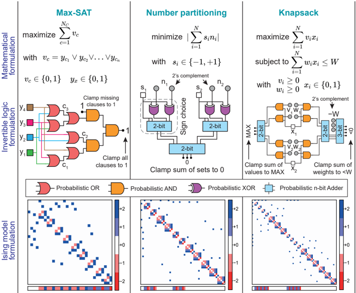</details> + + Fig. 6: Invertible logic encoding : The encoding process of three optimization problems, the maximum satisfiability problem (left column), number partitioning (central column), and the knapsack problem (right column), is streamlined and visually summarized into three steps: a problem first has to be condensed into a concise mathematical formulation (upper part of the image); then, an invertible Boolean circuit that topologically maps the problem is conceived; finally, the invertible Boolean circuit is converted into an Ising model using probabilistic AND/OR/NOT gates [14]. ## VI. ALGORITHMS AND APPLICATIONS ## A. Combinatorial Optimization via Invertible Logic When using the Ising model to solve an optimization problem, the first step is to provide a mapping between the Ising model and the problem to be solved. Early work on quantum annealing stimulated by D-Wave's quantum annealers generated a significant amount of useful research in this area [104], some of which are being adopted by quantuminspired classical annealers. There are usually many different ways to find a mapping, for example, some strategies may employ more nodes than others to encode the same instance, while others might result in graphs with topology unsuited to the computational architecture of choice. In this context, the invertible logic approach introduced in Ref. [12] stands out for its flexibility and sparse encodings. The process of mapping an instance into an Ising model can be broadly summarized into three steps, as illustrated by FIG. 6. In the figure, the steps of the invertible logic encoding of three combinatorial optimization problems, maximum satisfiability (left column), number partitioning (middle column), and knapsack (right column), are shown. First, each problem is formalized into a tight mathematical formulation (top row). Next, the problem is mapped into an invertible Boolean logic circuit (central row), meaning that each logic gate can be operated using any terminals as input/output nodes (similar to those discussed in the context of quantum annealing [105, 106] and memcomputing [107, 108]). Finally, the probabilistic circuit is algorithmically encoded into an Ising model (bottom row). Each logic gate has several Ising encodings that map the energy landscape of its logic operator. After the Boolean logic formulation of a problem, this step can be automated in standardized synthesis tools. The overall approach results in relatively sparse circuits, as illustrated in the bottom row of FIG. 6 where all three problems show similarly sparse matrices [W], with bias vectors { h } shown under. The key advantage of this approach, compared to heuristic and dense formulations of Ref. [104], is due to the generality of Boolean logic, quite similar to how present-day digital VLSI circuits are constructed in sparse, hardware-aware networks using billions of transistors. As such, much of the existing ecosystem of high-level synthesis can be directly used to find invertible logic-based encodings for general optimization problems. ## B. Machine Learning: energy-based models Energy-efficient machine learning (ML) with Boltzmann Machines (BMs) is a promising application for probabilistic computers with a recent experimental demonstration in Ref. [76]. Mainstream ML algorithms are designed and chosen with CPU implementation in mind and hence some models are heavily preferred over others even though they are often less powerful. For example, the use of RBMs over the more powerful unrestricted or deep BMs is motivated by the former's efficient software implementation in synchronous systems. 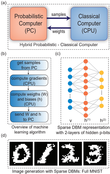However, by exploiting the technique of sparsity and massively parallel architecture described earlier, fast Gibbs sampling with DBMs + + + + + + Fig. 7: Generative neural networks with p-bits : (a) Hybrid computing scheme with probabilistic computer and classical computer is demonstrated where the probabilistic computer generates samples according to the weights given by CPU with a sampling speed of around 100 flips/ns. (b) shows the overview of the learning procedure for the hybrid set-up. Receiving the samples from the probabilistic computer, the CPU computes the gradient, updates the weights and biases, and sends them back to the probabilistic computer until converged. (c) Sparse Deep Boltzmann Machine (DBM) is utilized here as a hardware-aware graph that can be represented with multiple hidden layers of p-bits. Both inter-layer and intra-layer connections are allowed between visible and hidden units. (d) The images shown here are generated with a sparse DBM of 4264 p-bits after training the network with full MNIST. The label p-bits are clamped to a specific image and the network evolves to that image by annealing the system from β = 0 to β = 5 with a step size of 0.125. <details> <summary>Image 7 Details</summary>  ### Visual Description ## Diagram: Hybrid Probabilistic-Classical Computer System ### Overview The image presents a system diagram of a hybrid probabilistic-classical computer, a machine learning algorithm overview, a sparse Deep Boltzmann Machine (DBM) representation, and image generation results using sparse DBMs. It is divided into four sub-figures labeled (a), (b), (c), and (d). ### Components/Axes * **(a) Hybrid Probabilistic - Classical Computer:** * Two rectangular blocks represent the "Probabilistic Computer (PC)" (colored orange) and the "Classical Computer (CPU)" (colored blue). * Arrows indicate data flow: "samples" from PC to CPU, and "weights" from CPU to PC. * **(b) Overview of machine learning algorithm:** * A flowchart with four rounded rectangles, each representing a step in the algorithm. * "get samples from PC" * "compute gradients (CPU)" * "compute weights (W) and biases (h) (CPU)" * "send W and h to PC" * **(c) Sparse DBM representation with 2-layers of hidden p-bits:** * A neural network diagram with three layers of nodes. * Input layer 'v' (blue nodes). * First hidden layer 'h^(1)' (orange nodes). * Second hidden layer 'h^(2)' (yellow nodes). * Lines connect nodes between layers, representing connections/weights. * **(d) Image generation with Sparse DBMs: Full MNIST:** * Four black and white images, presumably generated digits from the MNIST dataset. The digits appear to be 0, 1, 2, and 3. ### Detailed Analysis * **(a)** The Probabilistic Computer (PC) and Classical Computer (CPU) exchange data. The PC sends samples to the CPU, and the CPU sends weights back to the PC. * **(b)** The machine learning algorithm involves getting samples from the PC, computing gradients and weights/biases using the CPU, and sending the weights/biases back to the PC. * **(c)** The Sparse DBM has an input layer (v) and two hidden layers (h^(1) and h^(2)). The connections between layers suggest a feedforward network. * **(d)** The generated images are pixelated representations of digits, indicating the DBM's ability to generate images. ### Key Observations * The system combines probabilistic and classical computing elements. * The machine learning algorithm is iterative, involving data exchange between the PC and CPU. * The DBM architecture has two hidden layers. * The generated images are recognizable as digits, demonstrating the model's learning capability. ### Interpretation The diagram illustrates a hybrid computing system where a probabilistic computer and a classical computer work together to perform machine learning tasks. The probabilistic computer likely provides samples for training, while the classical computer handles the computationally intensive tasks of gradient calculation and weight updates. The sparse DBM is used for image generation, and the results show that the model can learn to generate recognizable digits. The system leverages the strengths of both probabilistic and classical computing to achieve its goals. </details> can dramatically improve the state-of-the-art machine learning applications like visual object recognition and generation, speech recognition, autonomous driving, and many more [109]. Here we present an example where a sparse DBM is trained with MNIST handwritten digits (FIG. 7). We randomly distribute the visible and hidden units on the sparse DBM with massively parallel pseudo-asynchronous architecture which yields multiple hidden layers as shown in FIG. 7(c). Contrasting with earlier unconventional computing approaches where the MNIST dataset is reduced to much smaller sizes [110, 111], we show how the full MNIST dataset (60,000 images and no down-sampling) can be trained using p-computers in FPGAs. We use 1200 mini-batches having 50 images in each batch to train the network using the contrastive divergence (CD) algorithm. The process of learning is accomplished using a hybrid probabilistic and classical computer setup. The classical computer computes the gradients and generates new weights while the p-computer generates samples according to those weights (FIG. 7(b)). During the positive phase of sampling, the p-computer operates in its clamped condition under the direct influence of the training samples. In the negative phase, the p-computer is allowed to run freely without any environmental input. After training, the deep network not only can classify images but also generate images. For any given label, the network can create a new sample (not present in the training set) (FIG. 7(d)). This is an important feature of energy-based models and is commonly demonstrated with diffusion models [112]. ## C. Quantum simulation One primary motivation for building quantum computers is to simulate large quantum many-body systems and understand the exotic physics offered by them [113]. Two major challenges with quantum computers are the necessity of using cryogenic operating temperatures and the vulnerability to noise, rendering quantum computers impractical, especially considering practical overheads [114]. Simulating these systems with classical computers is often extremely time-consuming and mostly limited to small systems. One potential application of p-bits is to provide a room-temperature solution to boost the simulation speed and potentially enable the simulation of large-scale quantum systems. Significant progress has been made toward this end in recent years. ## 1) Simulating quantum systems with Trotterization One approach is to build a p-computer enabling the scalable simulation of sign-problem-free quantum systems by accelerating standard Quantum Monte Carlo (QMC) techniques [115]. The basic idea is to replace the qubits in the original lattice with hardware p-bits and replicate the new lattice according to the Suzuki-Trotter transformation [116]. Recently, the convergence time of a 2D square-octagonal qubit lattice initially prepared in a topologically obstructed state was compared among a CPU, a physical quantum annealer [117] and a pcomputer (both digital and analog) [118]. For this particular problem, it was shown that an FPGA-based p-computer emulator can be around 1000 times faster than an optimized C++ (CPU) program. Based on SPICE simulations of a small p-computer, we project that significant further acceleration should be possible with a truly asynchronous implementation. Probabilistic computers can be used for quantum Hamiltonians beyond the usual Transverse Field Ising Model, such as the antiferromagnetic Heisenberg Hamiltonian [119] and even for the emulation of gate-based quantum computers [120]. However, for generic Hamiltonians, (e.g., random circuit sampling), the number of samples required in naive implementations seem to grow exponentially [120] due to the notorious signproblem [121]. However, clever basis transformations [122] might mitigate or cure the sign-problem [123] in the future. ## 2) Machine learning quantum many-body systems With the great success of machine learning and AI algorithms, training stochastic neural networks (such as Boltzmann machines) to approximately solve the quantum many-body problem starting from a variational guess has generated great excitement [124-126] and is considered to be a fruitful combination of quantum physics and machine learning [127]. 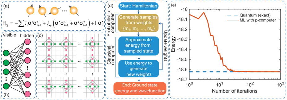These algorithms are typically implemented in high-level software programs, allowing users to choose from various network Fig. 8: Machine learning quantum systems with p-bits : (a) Heisenberg Hamiltonian with a transverse field ( Γ = +1 ) is applied to a FM coupled ( J Z = +1 and J xy = +0 . 5 ) linear chain of twelve ( 12 ) qubits with periodic boundary. (b) To obtain the ground state of this quantum system, a restricted Boltzmann machine is employed with 12 visible and 48 hidden nodes, where all nodes in the visible layer are connected to all nodes in the hidden layer. (c) This machine learning model is then embedded onto a hardware amenable sparse p-bit network arranged in a chimera graph using minor graph embedding. We use a coupling strength of 1.0 among the replicated visible and hidden nodes in the embedded p-bit network. (d) An overview of the machine learning algorithm and the division of workload between the probabilistic and classical computers in a hybrid setting is shown. (e) The FPGA emulation of this probabilistic computer performs variational machine learning in tandem with a classical computer, converging to the quantum (exact) result as shown. <details> <summary>Image 8 Details</summary>  ### Visual Description ## Composite Figure: Quantum Computing and Machine Learning ### Overview The image is a composite figure illustrating a quantum computing approach combined with machine learning. It includes a schematic of a quantum system, a neural network representation, a computational flow diagram, and a convergence plot comparing the energy of a quantum system calculated exactly versus using a machine learning approach with a probabilistic computer. ### Components/Axes * **(a) Quantum System Schematic:** * A series of spheres, presumably representing atoms or qubits, with arrows indicating spin directions. * Equation: H\_Q = - Σ J\_z σ^z\_i σ^z\_{i+1} + J\_{xy} (σ^x\_i σ^x\_{i+1} + σ^y\_i σ^y\_{i+1}) + Γ σ^x\_i * **(b) Neural Network Representation:** * "visible" layer: A column of green circles on the left. * "hidden" layer: A column of pink circles on the right. * Lines connecting each node in the visible layer to each node in the hidden layer. * **(c) Lattice Structure:** * A grid-like structure with repeating units. Each unit contains green and pink circles connected by lines. * **(d) Computational Flow Diagram:** * Divided into "Probabilistic computer" and "Classical computer" sections. * Flow: 1. Start: Hamiltonian (Blue rectangle) 2. Generate samples from weights {m1, m2, ..., mN} (Gold rectangle) 3. Approximate energy from sampled state (Blue rectangle) 4. Use energy to generate new weights (Blue rectangle) 5. Update weights (Arrow pointing back to step 2) 6. End: Ground state energy and wavefunction (Orange rectangle) * **(e) Convergence Plot:** * X-axis: Number of iterations (Logarithmic scale from 10^0 to 10^31) * Y-axis: Energy (Linear scale from -18.7 to -18) * Legend (Top-right): * Blue dashed line: Quantum (exact) * Red solid line: ML with p-computer ### Detailed Analysis * **(a) Quantum System:** * The equation represents a Hamiltonian, likely for an Ising-type model with transverse field. * J\_z and J\_{xy} are coupling constants. * σ^z, σ^x, and σ^y are Pauli matrices. * Γ represents the transverse field strength. * **(b) Neural Network:** * The network has a visible layer with approximately 5 nodes and a hidden layer with approximately 5 nodes. * The "..." indicates that the layers can have more nodes. * **(c) Lattice Structure:** * The lattice appears to be a 2D grid. * Each repeating unit has a diamond shape formed by the connections between green and pink circles. * **(d) Computational Flow:** * The algorithm iteratively refines the weights of a probabilistic computer using a classical computer to approximate the ground state energy. * **(e) Convergence Plot:** * The blue dashed line (Quantum (exact)) is a horizontal line at approximately -18.65. * The red solid line (ML with p-computer) starts at approximately -18.0 and rapidly decreases, converging to approximately -18.65 after about 10 iterations. * The x-axis is a log scale. ### Key Observations * The machine learning approach converges to the exact quantum result after a relatively small number of iterations. * The initial energy estimate from the machine learning approach is significantly higher than the exact quantum energy. * The algorithm effectively minimizes the energy by adjusting the weights of the probabilistic computer. ### Interpretation The figure demonstrates a hybrid quantum-classical approach to solving a quantum problem. The machine learning algorithm, implemented on a probabilistic computer, learns to approximate the ground state energy of a quantum system. The convergence plot shows that the machine learning approach can accurately reproduce the exact quantum result, suggesting that this hybrid approach could be a powerful tool for studying complex quantum systems. The neural network and lattice structure likely represent the underlying architecture used in the machine learning model. The computational flow diagram provides a clear overview of the algorithm's steps. </details> models and sizes according to their needs. However, as with classical machine learning, the difficulty of training strongly hinders the use of deeper and more general models. With scaled p-computers using millions of magnetic p-bits, massively parallel and energy-efficient hardware implementations of the more general unrestricted/deep BMs may become feasible, paving the way to simulate practical quantum systems. To demonstrate one such example of this approach, we show how p-bits laid out in sparse, hardware-aware graphs can be used for machine learning quantum systems (FIG. 8). The objective of this problem is to find the ground state of a many-body quantum system, in this case, a 1D FM Heisenberg Hamiltonian with an external transverse field. We start with an RBM, which is one of the simplest neural network models, and use its functional form as the variational guess for the ground state probabilities (the wavefunction is obtained by taking the square root of probabilities according to the Born rule). A combination of probabilistic sampling and weight updates gradually adjusts the variational guess such that the final guess points to the ground state of the quantum Hamiltonian. Emulating this variational ML approach with pbits requires a few more steps. An RBM network contains allto-all connections between the visible and hidden layers which is not conducive for scalable p-computers because of the large fanout demanded by the all-to-all connectivity. An alternative is to map the RBM onto a sparse graph through minor graph embedding [102]. Using a hybrid setup with fast sampling in a probabilistic computer coupled with a classical computer, the iterative process of sampling and weight updating can then be performed. The key advantage of having a massively parallel and fast sampler is the selection of higher-quality states of the wave function to update the variational guess. FIG. 8 shows an example simulation of how a p-computer learns the ground state of a 1D FM Heisenberg model. The scaling of p-computers using magnetic p-bits may allow much larger implementations of quantum systems in the future. ## D. Outlook: algorithms and applications beyond Despite the large range of applications we discussed in the context of p-bits, much of the sampling algorithms have been either standard MCMC or generic simulated annealing-based approaches. Future possibilities involve more sophisticated sampling and annealing algorithms such as parallel tempering (PT) (see Ref. [128, 129] for some initial investigations). Further improvements to hardware implementation include adaptive versions of PT [130] as well as sophisticated nonequilibrium Monte Carlo (NMC) algorithms [131]. Ideas involving overclocking p-bits such that they violate the t synapse 〈 T p-bit 〉 requirement for further improvement [14] or sharing synaptic operations between p-bits [82] could also be useful. A combination of these ideas with algorithm-architecture-device co-design may lead to orders of magnitude improvement in sampling speeds and quality. In this context, as a sampling throughput metric, increasing flips/ns is an important goal. In addition, solution quality, the possibility of cluster updates or algorithmic techniques also need to be considered carefully. Given the plethora of approaches from multiple communities, we also hope that model problems, benchmarking studies comparing different Ising machines, probabilistic accelerators, physical annealers and dynamical solvers will be performed in the near future from all practitioners, including ourselves. We believe that the co-design of algorithms, architectures, and devices for probabilistic computing may not only help mitigate the looming energy crisis of machine learning and AI but also lead to systems which may unlock previously inaccessible regimes using powerful probabilistic (randomized) algorithms [132]. Just as the emergence of powerful GPUs made the well-known backpropagation algorithm flourish, probabilistic computers could lead us to the previously unknown territory of energy-based AI models, combinatorial optimization and quantum simulation. This research program requires a concerted effort and interdisciplinary expertise from all across the stack and ties into the larger vision of unconventional computing forming in the community [133]. ## REFERENCES - [1] D. Patterson, J. Gonzalez, Q. Le, C. Liang, L.-M. Munguia, D. Rothchild, D. So, M. Texier, and J. Dean, 'Carbon emissions and large neural network training,' arXiv preprint arXiv:2104.10350 , 2021. - [2] S. Sudhakar, V. Sze, and S. Karaman, 'Data centers on wheels: Emissions from computing onboard autonomous vehicles,' IEEE Micro , vol. 43, no. 1, pp. 29-39, 2022. - [3] R. Chau, 'Process and packaging innovations for moore's law continuation and beyond,' in 2019 IEEE International Electron Devices Meeting (IEDM) . IEEE, 2019, pp. 1-1. - [4] J. C. Wong and S. Salahuddin, 'Negative capacitance transistors,' Proceedings of the IEEE , vol. 107, no. 1, pp. 49-62, 2018. - [5] M. A. Alam, M. Si, and P. D. Ye, 'A critical review of recent progress on negative capacitance field-effect transistors,' Applied Physics Letters , vol. 114, no. 9, p. 090401, 2019. - [6] S. Manipatruni, D. E. Nikonov, C.-C. Lin, T. A. Gosavi, H. Liu, B. Prasad, Y.-L. Huang, E. Bonturim, R. Ramesh, and I. A. Young, 'Scalable energy-efficient magnetoelectric spin-orbit logic,' Nature , vol. 565, no. 7737, pp. 35-42, 2019. - [7] P. Debashis, J. Plombon, C.-C. Lin, Y.-C. Liao, H. Li, D. Nikonov, D. Adams, C. Rogan, M. DC, M. Radosavljevic, S. Clendenning, I. Young, and I. Corporation, 'Low-voltage and high-speed switching of a magnetoelectric element for energy efficient compute,' in 2022 IEEE International Electron Devices Meeting (IEDM) , 2022. - [8] A. Chen, 'Emerging research device roadmap and perspectives,' in 2014 IEEE International Conference on IC Design & Technology . IEEE, 2014, pp. 1-4. - [9] G. Finocchio, M. Di Ventra, K. Y. Camsari, K. Everschor-Sitte, P. Khalili Amiri, and Z. Zeng, 'The promise of spintronics for unconventional computing,' Journal of Magnetism and Magnetic Materials , vol. 521, p. 167506, 2021. - [10] B. Behin-Aein, V. Diep, and S. Datta, 'A building block for hardware belief networks,' Scientific reports , vol. 6, no. 1, pp. 1-10, 2016. - [11] B. Sutton, K. Y. Camsari, B. Behin-Aein, and S. Datta, 'Intrinsic optimization using stochastic nanomagnets,' Scientific Reports , vol. 7, p. 44370, 2017. - [12] K. Y. Camsari, R. Faria, B. M. Sutton, and S. Datta, 'Stochastic p-bits for invertible logic,' Physical Review X , vol. 7, no. 3, p. 031014, 2017. - [13] R. P. Feynman, 'Simulating physics with computers,' International journal of theoretical physics , vol. 21, no. 6-7, pp. 467-488, 1982. - [14] N. A. Aadit, A. Grimaldi, M. Carpentieri, L. Theogarajan, J. M. Martinis, G. Finocchio, and K. Y. Camsari, 'Massively parallel probabilistic computing with sparse ising machines,' Nature Electronics , pp. 1-9, 2022. - [15] J. Kaiser, R. Jaiswal, B. Behin-Aein, and S. Datta, 'Benchmarking a probabilistic coprocessor,' arXiv preprint arXiv:2109.14801 , 2021. - [16] S. Misra, L. C. Bland, S. G. Cardwell, J. A. C. Incorvia, C. D. James, A. D. Kent, C. D. Schuman, J. D. Smith, and J. B. Aimone, 'Probabilistic neural computing with stochastic devices,' Advanced Materials , p. 2204569, 2022. - [17] P. J. Coles, 'Thermodynamic ai and the fluctuation frontier,' arXiv preprint arXiv:2302.06584 , 2023. - [18] W. A. Borders, A. Z. Pervaiz, S. Fukami, K. Y. Camsari, H. Ohno, and S. Datta, 'Integer factorization using stochastic magnetic tunnel junctions,' Nature , 2019. - [19] R. Faria, J. Kaiser, K. Y. Camsari, and S. Datta, 'Hardware design for autonomous bayesian networks,' Frontiers in computational neuroscience , vol. 15, p. 14, 2021. - [20] E. Aarts and J. Korst, Simulated annealing and Boltzmann machines: a stochastic approach to combinatorial optimization and neural computing . John Wiley & Sons, Inc., 1989. - [21] A. Houshang, M. Zahedinejad, S. Muralidhar, J. Checinski, A. A. Awad, and J. ˚ Akerman, 'A spin hall ising machine,' arXiv preprint arXiv:2006.02236 , 2020. - [22] Y. Su, J. Mu, H. Kim, and B. Kim, 'A scalable cmos ising computer featuring sparse and reconfigurable spin interconnects for solving combinatorial optimization problems,' IEEE Journal of Solid-State Circuits , vol. 57, no. 3, pp. 858-868, 2022. - [23] S. Bhanja, D. Karunaratne, R. Panchumarthy, S. Rajaram, and S. Sarkar, 'Non-boolean computing with nanomagnets for computer vision applications,' Nature nanotechnology , vol. 11, no. 2, pp. 177-183, 2016. - [24] P. Debashis, R. Faria, K. Y. Camsari, J. Appenzeller, S. Datta, and Z. Chen, 'Experimental demonstration of nanomagnet networks as hardware for ising computing,' in Electron Devices Meeting (IEDM), 2016 IEEE International . IEEE, 2016, pp. 34-3. - [25] P. L. McMahon et al., 'A fully programmable 100spin coherent ising machine with all-to-all connections,' Science , vol. 354, no. 6312, pp. 614-617, 2016. - [26] S. Dutta, A. Khanna, A. Assoa, H. Paik, D. G. Schlom, Z. Toroczkai, A. Raychowdhury, and S. Datta, 'An ising hamiltonian solver based on coupled stochastic phasetransition nano-oscillators,' Nature Electronics , vol. 4, no. 7, pp. 502-512, 2021. - [27] J. Chou, S. Bramhavar, S. Ghosh, and W. Herzog, 'Analog coupled oscillator based weighted ising machine,' Scientific reports , vol. 9, no. 1, pp. 1-10, 2019. - [28] M. Yamaoka et al., 'A 20k-spin ising chip to solve combinatorial optimization problems with cmos annealing,' IEEE Journal of Solid-State Circuits , vol. 51, no. 1, pp. 303-309, 2016. - [29] T. Wang and J. Roychowdhury, 'Oim: Oscillator-based ising machines for solving combinatorial optimisation problems,' in International Conference on Unconventional Computation and Natural Computation . Springer, 2019, pp. 232-256. - [30] Y. Shim, A. Jaiswal, and K. Roy, 'Ising computation based combinatorial optimization using spin-hall effect (she) induced stochastic magnetization reversal,' Journal of Applied Physics , vol. 121, no. 19, p. 193902, 2017. - [31] T. Inagaki et al., 'A coherent ising machine for 2000node optimization problems,' Science , vol. 354, no. 6312, pp. 603-606, 2016. - [32] M. Baity-Jesi, R. A. Ba˜ nos, A. Cruz, L. A. Fernandez, J. M. Gil-Narvi´ on, A. Gordillo-Guerrero, D. I˜ niguez, A. Maiorano, F. Mantovani, E. Marinari et al. , 'Janus ii: A new generation application-driven computer for spin-system simulations,' Computer Physics Communications , vol. 185, no. 2, pp. 550-559, 2014. - [33] M. Yamaoka, C. Yoshimura, M. Hayashi, T. Okuyama, H. Aoki, and H. Mizuno, '24.3 20k-spin ising chip for combinational optimization problem with cmos annealing,' in 2015 IEEE International Solid-State Circuits Conference-(ISSCC) Digest of Technical Papers . IEEE, 2015, pp. 1-3. - [34] N. G. Berloff, M. Silva, K. Kalinin, A. Askitopoulos, J. D. T¨ opfer, P. Cilibrizzi, W. Langbein, and P. G. Lagoudakis, 'Realizing the classical xy hamiltonian in polariton simulators,' Nature materials , vol. 16, no. 11, pp. 1120-1126, 2017. - [35] T. Takemoto, M. Hayashi, C. Yoshimura, and M. Yamaoka, '2.6 a 2 × 30k-spin multichip scalable annealing processor based on a processing-in-memory approach for solving large-scale combinatorial optimization problems,' in 2019 IEEE International Solid-State Circuits Conference-(ISSCC) . IEEE, 2019, pp. 52-54. - [36] H. Goto, K. Tatsumura, and A. R. Dixon, 'Combinatorial optimization by simulating adiabatic bifurcations in nonlinear hamiltonian systems,' Science advances , vol. 5, no. 4, p. eaav2372, 2019. - [37] M. Aramon, G. Rosenberg, E. Valiante, T. Miyazawa, H. Tamura, and H. G. Katzgraber, 'Physics-inspired optimization for quadratic unconstrained problems using a digital annealer,' Frontiers in Physics , vol. 7, p. 48, 2019. - [38] A. Mallick, M. K. Bashar, D. S. Truesdell, B. H. Calhoun, S. Joshi, and N. Shukla, 'Using synchronized oscillators to compute the maximum independent set,' Nature communications , vol. 11, no. 1, pp. 1-7, 2020. - [39] K. Yamamoto, K. Ando, N. Mertig, T. Takemoto, M. Yamaoka, H. Teramoto, A. Sakai, S. TakamaedaYamazaki, and M. Motomura, '7.3 statica: A 512-spin 0.25 m-weight full-digital annealing processor with a near-memory all-spin-updates-at-once architecture for combinatorial optimization with complete spin-spin interactions,' in 2020 IEEE International Solid-State Circuits Conference-(ISSCC) . IEEE, 2020, pp. 138-140. - [40] S. Patel, P. Canoza, and S. Salahuddin, 'Logically synthesized and hardware-accelerated restricted boltzmann machines for combinatorial optimization and integer factorization,' Nature Electronics , vol. 5, no. 2, pp. 92101, 2022. - [41] R. Afoakwa, Y. Zhang, U. K. R. Vengalam, Z. Ignja- tovic, and M. Huang, 'Cmos ising machines with coupled bistable nodes,' arXiv preprint arXiv:2007.06665 , 2020. - [42] A. Lu, J. Hur, Y.-C. Luo, H. Li, D. E. Nikonov, I. Young, Y.-K. Choi, and S. Yu, 'Scalable in-memory clustered annealer with temporal noise of finfet for the travelling salesman problem,' in 2022 International Electron Devices Meeting (IEDM) . IEEE, 2022, pp. 22-5. - [43] W. Moy, I. Ahmed, P.-w. Chiu, J. Moy, S. S. Sapatnekar, and C. H. Kim, 'A 1,968-node coupled ring oscillator circuit for combinatorial optimization problem solving,' Nature Electronics , vol. 5, no. 5, pp. 310-317, 2022. - [44] N. Mohseni, P. L. McMahon, and T. Byrnes, 'Ising machines as hardware solvers of combinatorial optimization problems,' Nature Reviews Physics , vol. 4, no. 6, pp. 363-379, may 2022. - [45] M. Marsman, G. Maris, T. Bechger, and C. Glas, 'Bayesian inference for low-rank ising networks,' Scientific Reports , vol. 5, no. 1, mar 2015. - [46] M. T. McCray, M. A. Abeed, and S. Bandyopadhyay, 'Electrically programmable probabilistic bit anticorrelator on a nanomagnetic platform,' Scientific reports , vol. 10, no. 1, pp. 1-11, 2020. - [47] P. Debashis, V. Ostwal, R. Faria, S. Datta, J. Appenzeller, and Z. Chen, 'Hardware implementation of bayesian network building blocks with stochastic spintronic devices,' Scientific reports , vol. 10, no. 1, p. 16002, 2020. - [48] S. Nasrin, J. Drobitch, P. Shukla, T. Tulabandhula, S. Bandyopadhyay, and A. R. Trivedi, 'Bayesian reasoning machine on a magneto-tunneling junction network,' Nanotechnology , vol. 31, no. 48, p. 484001, 2020. - [49] K.-E. Harabi, T. Hirtzlin, C. Turck, E. Vianello, R. Laurent, J. Droulez, P. Bessi` ere, J.-M. Portal, M. Bocquet, and D. Querlioz, 'A memristor-based bayesian machine,' Nature Electronics , pp. 1-12, 2022. - [50] M. G. Morshed, S. Ganguly, and A. W. Ghosh, 'A deep dive into the computational fidelity of high variability low energy barrier magnet technology for accelerating optimization and bayesian problems,' 2023. [Online]. Available: https://arxiv.org/abs/2302.08074 - [51] C. Bybee, D. Kleyko, D. E. Nikonov, A. Khosrowshahi, B. A. Olshausen, and F. T. Sommer, 'Efficient optimization with higher-order ising machines,' arXiv preprint arXiv:2212.03426 , 2022. - [52] M. K. Bashar and N. Shukla, 'Constructing dynamical systems to model higher order ising spin interactions and their application in solving combinatorial optimization problems,' arXiv preprint arXiv:2211.05365 , 2022. - [53] N. Onizawa and T. Hanyu, 'High convergence rates of cmos invertible logic circuits based on many-body hamiltonians,' in 2021 IEEE International Symposium on Circuits and Systems (ISCAS) . IEEE, 2021, pp. 1-5. - [54] B. Sutton, R. Faria, L. A. Ghantasala, R. Jaiswal, K. Y. Camsari, and S. Datta, 'Autonomous probabilistic coprocessing with petaflips per second,' IEEE Access , vol. 8, pp. 157 238-157 252, 2020. - [55] J. Kaiser and S. Datta, 'Probabilistic computing with p-bits,' Applied Physics Letters , vol. 119, no. 15, p. 150503, 2021. - [56] S. Aggarwal, H. Almasi, M. DeHerrera, B. Hughes, S. Ikegawa, J. Janesky, H. Lee, H. Lu, F. Mancoff, K. Nagel et al. , 'Demonstration of a reliable 1 gb standalone spin-transfer torque mram for industrial applications,' in 2019 IEEE International Electron Devices Meeting (IEDM) . IEEE, 2019, pp. 2-1. - [57] K. Lee, J. Bak, Y. Kim, C. Kim, A. Antonyan, D. Chang, S. Hwang, G. Lee, N. Ji, W. Kim et al. , '1gbit high density embedded stt-mram in 28nm fdsoi technology,' in 2019 IEEE International Electron Devices Meeting (IEDM) . IEEE, 2019, pp. 2-2. - [58] J. L. Drobitch and S. Bandyopadhyay, 'Reliability and scalability of p-bits implemented with low energy barrier nanomagnets,' IEEE Magnetics Letters , vol. 10, pp. 1-4, 2019. - [59] R. Rahman and S. Bandyopadhyay, 'Variability of binary stochastic neurons employing low energy barrier nanomagnets with in-plane anisotropy,' 2021. [Online]. Available: https://arxiv.org/abs/2108.04319 - [60] O. Hassan, S. Datta, and K. Y. Camsari, 'Quantitative evaluation of hardware binary stochastic neurons,' Physical Review Applied , vol. 15, no. 6, p. 064046, 2021. - [61] K. Y. Camsari, M. M. Torunbalci, W. A. Borders, H. Ohno, and S. Fukami, 'Double-free-layer magnetic tunnel junctions for probabilistic bits,' Physical Review Applied , vol. 15, no. 4, p. 044049, 2021. - [62] R. Rahman and S. Bandyopadhyay, 'Robustness of binary stochastic neurons implemented with low barrier nanomagnets made of dilute magnetic semiconductors,' IEEE Magnetics Letters , vol. 13, pp. 1-4, 2022. - [63] Y. Lv, R. P. Bloom, and J.-P. Wang, 'Experimental demonstration of probabilistic spin logic by magnetic tunnel junctions,' IEEE Magnetics Letters , vol. 10, pp. 1-5, 2019. - [64] K. Y. Camsari, P. Debashis, V. Ostwal, A. Z. Pervaiz, T. Shen, Z. Chen, S. Datta, and J. Appenzeller, 'From charge to spin and spin to charge: Stochastic magnets for probabilistic switching,' Proceedings of the IEEE , vol. 108, no. 8, pp. 1322-1337, 2020. - [65] X. Chen, J. Zhang, J. Xiao et al. , 'Magnetic-tunneljunction-based true random-number generator with enhanced generation rate,' Physical Review Applied , vol. 18, no. 2, p. L021002, 2022. - [66] L. Rehm, C. C. M. Capriata, M. Shashank, J. D. Smith, M. Pinarbasi, B. G. Malm, and A. D. Kent, 'Stochastic magnetic actuated random transducer devices based on perpendicular magnetic tunnel junctions,' arXiv preprint arXiv:2209.01480 , 2022. - [67] B. R. Zink, Y. Lv, and J.-P. Wang, 'Review of magnetic tunnel junctions for stochastic computing,' IEEE Journal on Exploratory Solid-State Computational Devices and Circuits , vol. 8, no. 2, pp. 173-184, dec 2022. - [68] A. Fukushima, T. Seki, K. Yakushiji, H. Kubota, H. Imamura, S. Yuasa, and K. Ando, 'Spin dice: A scalable truly random number generator based on spintronics,' Applied Physics Express , vol. 7, no. 8, p. 083001, 2014. - [69] Y. Shao, S. L. Sinaga, I. O. Sunmola, A. S. Borland, M. J. Carey, J. A. Katine, V. Lopez-Dominguez, and P. K. Amiri, 'Implementation of artificial neural networks using magnetoresistive random-access memorybased stochastic computing units,' IEEE Magnetics Letters , vol. 12, pp. 1-5, 2021. - [70] K. Y. Camsari, S. Salahuddin, and S. Datta, 'Implementing p-bits with embedded mtj,' IEEE Electron Device Letters , vol. 38, no. 12, pp. 1767-1770, 2017. - [71] J. Kaiser, A. Rustagi, K. Y. Camsari, J. Z. Sun, S. Datta, and P. Upadhyaya, 'Subnanosecond fluctuations in lowbarrier nanomagnets,' Physical Review Applied , vol. 12, no. 5, p. 054056, 2019. - [72] O. Hassan, R. Faria, K. Y. Camsari, J. Z. Sun, and S. Datta, 'Low-barrier magnet design for efficient hardware binary stochastic neurons,' IEEE Magnetics Letters , vol. 10, pp. 1-5, 2019. - [73] K. Hayakawa, S. Kanai, T. Funatsu, J. Igarashi, B. Jinnai, W. Borders, H. Ohno, and S. Fukami, 'Nanosecond random telegraph noise in in-plane magnetic tunnel junctions,' Physical Review Letters , vol. 126, no. 11, p. 117202, 2021. - [74] C. Safranski, J. Kaiser, P. Trouilloud, P. Hashemi, G. Hu, and J. Z. Sun, 'Demonstration of nanosecond operation in stochastic magnetic tunnel junctions,' Nano Letters , vol. 21, no. 5, pp. 2040-2045, feb 2021. - [75] S. Kanai, K. Hayakawa, H. Ohno, and S. Fukami, 'Theory of relaxation time of stochastic nanomagnets,' Phys. Rev. B , vol. 103, p. 094423, Mar 2021. [Online]. Available: https://link.aps.org/doi/10.1103/PhysRevB.103.094423 - [76] J. Kaiser, W. A. Borders, K. Y. Camsari, S. Fukami, H. Ohno, and S. Datta, 'Hardware-aware in situ learning based on stochastic magnetic tunnel junctions,' Physical Review Applied , vol. 17, no. 1, p. 014016, 2022. - [77] A. Grimaldi, K. Selcuk, N. A. Aadit, K. Kobayashi, Q. Cao, S. Chowdhury, G. Finocchio, S. Kanai, H. Ohno, S. Fukami, and K. Y. Camsari, 'Experimental evaluation of simulated quantum annealing with mtjaugmented p-bits,' in 2022 IEEE International Electron Devices Meeting (IEDM) , 2022. - [78] J. Yin, Y. Liu, B. Zhang, A. Du, T. Gao, X. Ma, Y. Dong, Y. Bai, S. Lu, Y. Zhuo, Y. Huang, W. Cai, D. Zhu, K. Shi, K. Cao, D. Zhang, L. Zeng, and W. Zhao, 'Scalable ising computer based on ultra-fast field-free spin orbit torque stochastic device with extreme 1-bit quantization,' in 68th International Electron Devices Meeting (IEDM) , 2022. - [79] G. M. Guti´ errez-Finol, S. Gim´ enez-Santamarina, Z. Hu, L. E. Rosaleny, S. Cardona-Serra, and A. Gaita-Ari˜ no, 'Lanthanide molecular nanomagnets as probabilistic bits,' 2023. [Online]. Available: https://arxiv.org/abs/ 2301.08182 - [80] K. S. Woo, J. Kim, J. Han, W. Kim, Y. H. Jang, and C. S. Hwang, 'Probabilistic computing using cu0. 1te0. 9/hfo2/pt diffusive memristors,' Nature Communications , vol. 13, no. 1, p. 5762, 2022. - [81] Y. Liu, Q. Hu, Q. Wu, X. Liu, Y. Zhao, D. Zhang, Z. Han, J. Cheng, Q. Ding, Y. Han et al. , 'Probabilistic circuit implementation based on p-bits using the intrinsic random property of rram and p-bit multiplexing strategy,' Micromachines , vol. 13, no. 6, p. 924, 2022. - [82] T. J. Park, K. Selcuk, H.-T. Zhang, S. Manna, R. Batra, Q. Wang, H. Yu, N. A. Aadit, S. K. Sankaranarayanan, H. Zhou et al. , 'Efficient probabilistic computing with stochastic perovskite nickelates,' Nano Letters , vol. 22, no. 21, pp. 8654-8661, 2022. - [83] S. Cheemalavagu, P. Korkmaz, K. V. Palem, B. E. Akgul, and L. N. Chakrapani, 'A probabilistic cmos switch and its realization by exploiting noise,' in IFIP International Conference on VLSI , 2005, pp. 535-541. - [84] W. Whitehead, Z. Nelson, K. Y. Camsari, and L. Theogarajan, 'Cmos-compatible ising and potts annealing using single photon avalanche diodes,' arXiv preprint arXiv:2211.12607 , 2022. - [85] L. Xia, P. Gu, B. Li, T. Tang, X. Yin, W. Huangfu, S. Yu, Y. Cao, Y. Wang, and H. Yang, 'Technological exploration of rram crossbar array for matrix-vector multiplication,' Journal of Computer Science and Technology , vol. 31, no. 1, pp. 3-19, 2016. - [86] Y. Li, S. Kim, X. Sun, P. Solomon, T. Gokmen, H. Tsai, S. Koswatta, Z. Ren, R. Mo, C. C. Yeh et al. , 'Capacitor-based cross-point array for analog neural network with record symmetry and linearity,' in 2018 IEEE Symposium on VLSI Technology . IEEE, 2018, pp. 25-26. - [87] O. Hassan, K. Y. Camsari, and S. Datta, 'Voltage-driven building block for hardware belief networks,' IEEE Design & Test , vol. 36, no. 3, pp. 15-21, 2019. - [88] M. Kang, S. K. Gonugondla, A. Patil, and N. R. Shanbhag, 'A multi-functional in-memory inference processor using a standard 6t sram array,' IEEE Journal of Solid-State Circuits , vol. 53, no. 2, pp. 642-655, 2018. - [89] N. Verma, H. Jia, H. Valavi, Y. Tang, M. Ozatay, L.-Y. Chen, B. Zhang, and P. Deaville, 'In-memory computing: Advances and prospects,' IEEE Solid-State Circuits Magazine , vol. 11, no. 3, pp. 43-55, 2019. - [90] S. Geman and D. Geman, 'Stochastic relaxation, gibbs distributions, and the bayesian restoration of images,' IEEE Transactions on pattern analysis and machine intelligence , no. 6, pp. 721-741, 1984. - [91] D. Koller and N. Friedman, Probabilistic graphical models: principles and techniques . MIT press, 2009. - [92] G. E. Hinton, A Practical Guide to Training Restricted Boltzmann Machines . Berlin, Heidelberg: Springer Berlin Heidelberg, 2012, pp. 599-619. - [93] M. R. Garey and D. S. Johnson, Computers and intractability . freeman San Francisco, 1979, vol. 174. - [94] D. Br´ elaz, 'New methods to color the vertices of a graph,' Communications of the ACM , vol. 22, no. 4, pp. 251-256, apr 1979. - [95] Y. F. et al., 'Parallel tempering simulation of the three-dimensional edwards-anderson model with compact asynchronous multispin coding on gpu,' Computer Physics Communications , vol. 185, no. 10, pp. 2467 2478, 2014. - [96] K. Yang, Y.-F. Chen, G. Roumpos, C. Colby, and J. Anderson, 'High performance monte carlo simulation of ising model on tpu clusters,' in Proceedings of the International Conference for High Performance Computing, Networking, Storage and Analysis , 2019, pp. 115. - [97] P. Debashis, R. Faria, K. Y. Camsari, S. Datta, and Z. Chen, 'Correlated fluctuations in spin orbit torque coupled perpendicular nanomagnets,' Physical Review B , vol. 101, no. 9, p. 094405, 2020. - [98] N. A. Aadit, A. Grimaldi, G. Finocchio, and K. Y. Camsari, 'Physics-inspired ising computing with ring oscillator activated p-bits,' in 2022 IEEE 22nd International Conference on Nanotechnology (NANO) , 2022, pp. 393-396. - [99] S. Bhatti, R. Sbiaa, A. Hirohata, H. Ohno, S. Fukami, and S. Piramanayagam, 'Spintronics based random access memory: a review,' Materials Today , vol. 20, no. 9, pp. 530-548, 2017. - [100] H. Hoos and T. St¨ utzle, SATLIB: An online resource for research on SAT . IOS Press, 04 2000, pp. 283-292. - [101] A. Z. Pervaiz, L. A. Ghantasala, K. Y. Camsari, and S. Datta, 'Hardware emulation of stochastic p-bits for invertible logic,' Scientific reports , vol. 7, no. 1, p. 10994, 2017. - [102] V. Choi, 'Minor-embedding in adiabatic quantum computation: Ii. minor-universal graph design,' Quantum Information Processing , vol. 10, no. 3, pp. 343-353, 2011. - [103] N. Sagan and J. Roychowdhury, 'Das: Implementing dense ising machines using sparse resistive networks,' in Proceedings of the 41st IEEE/ACM International Conference on Computer-Aided Design , 2022, pp. 19. - [104] A. Lucas, 'Ising formulations of many np problems,' Frontiers in Physics , vol. 2, p. 5, 2014. - [105] E. Andriyash, Z. Bian, F. Chudak, M. Drew-Brook, A. D. King, W. G. Macready, and A. Roy, 'Boosting integer factoring performance via quantum annealing offsets,' D-Wave Technical Report Series , vol. 14, no. 2016, 2016. - [106] J. Biamonte, 'Nonperturbative k-body to two-body commuting conversion hamiltonians and embedding problem instances into ising spins,' Physical Review A , vol. 77, no. 5, p. 052331, 2008. - [107] F. L. Traversa and M. Di Ventra, 'Polynomial-time solution of prime factorization and np-complete problems with digital memcomputing machines,' Chaos: An Interdisciplinary Journal of Nonlinear Science , vol. 27, no. 2, p. 023107, 2017. - [108] M. Di Ventra, MemComputing: Fundamentals and Applications . Oxford University Press, 2022. - [109] R. Salakhutdinov and G. Hinton, 'Deep boltzmann machines,' in Proceedings of the Twelth International Conference on Artificial Intelligence and Statistics , ser. Proceedings of Machine Learning Research, D. van Dyk and M. Welling, Eds., vol. 5. Hilton Clearwater Beach Resort, Clearwater Beach, Florida USA: PMLR, 16-18 Apr 2009, pp. 448-455. [Online]. Available: https://proceedings.mlr.press/v5/salakhutdinov09a.html - [110] S. H. Adachi and M. P. Henderson, 'Application of quantum annealing to training of deep neural networks,' arXiv preprint arXiv:1510.06356 , 2015. - [111] H. Manukian, F. L. Traversa, and M. Di Ventra, 'Accelerating deep learning with memcomputing,' Neural Networks , vol. 110, pp. 1-7, 2019. - [112] J. Sohl-Dickstein, E. Weiss, N. Maheswaranathan, and S. Ganguli, 'Deep unsupervised learning using nonequilibrium thermodynamics,' in International Conference on Machine Learning . PMLR, 2015, pp. 2256-2265. - [113] H. Ma, M. Govoni, and G. Galli, 'Quantum simulations of materials on near-term quantum computers,' npj Computational Materials , vol. 6, no. 1, p. 85, 2020. - [114] R. Babbush, J. R. McClean, M. Newman, C. Gidney, S. Boixo, and H. Neven, 'Focus beyond quadratic speedups for error-corrected quantum advantage,' PRX Quantum , vol. 2, no. 1, p. 010103, 2021. - [115] K. Y. Camsari, S. Chowdhury, and S. Datta, 'Scalable emulation of sign-problem-free hamiltonians with room-temperature p-bits,' Physical Review Applied , vol. 12, no. 3, p. 034061, 2019. - [116] M. Suzuki, 'Relationship between d-dimensional quantal spin systems and (d+ 1)-dimensional ising systems: Equivalence, critical exponents and systematic approximants of the partition function and spin correlations,' Progress of theoretical physics , vol. 56, no. 5, pp. 14541469, 1976. - [117] A. D. King, J. Raymond, T. Lanting, S. V. Isakov, M. Mohseni, G. Poulin-Lamarre, S. Ejtemaee, W. Bernoudy, I. Ozfidan, A. Y. Smirnov et al. , 'Scaling advantage over path-integral monte carlo in quantum simulation of geometrically frustrated magnets,' Nature communications , vol. 12, no. 1, pp. 1-6, 2021. - [118] S. Chowdhury, K. Y. Camsari, and S. Datta, 'Accelerated quantum monte carlo with probabilistic computers,' 2022. [Online]. Available: https://arxiv.org/abs/2210.17526 - [119] S. Chowdhury, S. Datta, and K. Camsari, 'A probabilistic approach to quantum inspired algorithms,' in 2019 IEEE International Electron Devices Meeting (IEDM) . IEEE, 2019, pp. 37-5. - [120] S. Chowdhury, K. Y. Camsari, and S. Datta, 'Emulating quantum interference with generalized ising machines,' arXiv preprint arXiv:2007.07379 , 2020. - [121] M. Troyer et al., 'Computational complexity and fundamental limitations to fermionic quantum monte carlo simulations,' Physical review letters , vol. 94, no. 17, p. 170201, 2005. - [122] D. Aharonov, X. Gao, Z. Landau, Y. Liu, and U. Vazirani, 'A polynomial-time classical algorithm for noisy random circuit sampling,' arXiv preprint arXiv:2211.03999 , 2022. - [123] D. Hangleiter, I. Roth, D. Nagaj, and J. Eisert, 'Easing the monte carlo sign problem,' Science advances , vol. 6, no. 33, p. eabb8341, 2020. - [124] G. Carleo and M. Troyer, 'Solving the quantum manybody problem with artificial neural networks,' Science , vol. 355, no. 6325, pp. 602-606, 2017. - [125] Z. Cai and J. Liu, 'Approximating quantum manybody wave functions using artificial neural networks,' Phys. Rev. B , vol. 97, p. 035116, Jan 2018. [Online]. Available: https://link.aps.org/doi/10.1103/ PhysRevB.97.035116 - [126] H. Saito and M. Kato, 'Machine learning technique to find quantum many-body ground states of bosons on a lattice,' Journal of the Physical Society of Japan , vol. 87, no. 1, p. 014001, 2018. [Online]. Available: https://doi.org/10.7566/JPSJ.87.014001 - [127] S. D. Sarma, D.-L. Deng, and L.-M. Duan, 'Machine learning meets quantum physics,' arXiv preprint arXiv:1903.03516 , 2019. - [128] N. A. Aadit, A. Grimaldi, M. Carpentieri, L. Theogarajan, G. Finocchio, and K. Y. Camsari, 'Computing with invertible logic: Combinatorial optimization with probabilistic bits,' in 2021 IEEE International Electron Devices Meeting (IEDM) . IEEE, 2021, pp. 40-3. - [129] A. Grimaldi, L. S´ anchez-Tejerina, N. A. Aadit, S. Chiappini, M. Carpentieri, K. Camsari, and G. Finocchio, 'Spintronics-compatible approach to solving maximumsatisfiability problems with probabilistic computing, invertible logic, and parallel tempering,' Physical Review Applied , vol. 17, no. 2, p. 024052, 2022. - [130] G. Desjardins, A. Courville, and Y. Bengio, 'Adaptive parallel tempering for stochastic maximum likelihood learning of rbms,' arXiv preprint arXiv:1012.3476 , 2010. - [131] M. Mohseni, D. Eppens, J. Strumpfer, R. Marino, V. Denchev, A. K. Ho, S. V. Isakov, S. Boixo, F. RicciTersenghi, and H. Neven, 'Nonequilibrium monte carlo for unfreezing variables in hard combinatorial optimization,' arXiv preprint arXiv:2111.13628 , 2021. - [132] A. Buluc, T. G. Kolda, S. M. Wild, M. Anitescu, A. DeGennaro, J. Jakeman, C. Kamath, M. E. Lopes, P.-G. Martinsson, K. Myers et al. , 'Randomized algorithms for scientific computing (rasc),' arXiv preprint arXiv:2104.11079 , 2021. - [133] G. Finocchio, S. Bandyopadhyay, P. Lin, G. Pan, J. J. Yang, R. Tomasello, C. Panagopoulos, M. Carpentieri, V. Puliafito, J. ˚ Akerman et al. , 'Roadmap for unconventional computing with nanotechnology,' arXiv preprint arXiv:2301.06727 , 2023.