# Associated quarkonia production in a single boson e+e−superscript𝑒superscript𝑒e^{+}e^{-}italic_e start_POSTSUPERSCRIPT + end_POSTSUPERSCRIPT italic_e start_POSTSUPERSCRIPT - end_POSTSUPERSCRIPT annihilation
**Authors**: I. N. Belov, A. V. Berezhnoy, E. A. Leshchenko
> INFN, Sezione di Genova, Italy
> SINP MSU, Moscow, Russia
> Physics department of MSU, Moscow, Russia
nonumber
## Abstract
The production cross sections of charmonia, charmonium-bottomonium and bottomonia pairs in a single boson $e^{+}e^{-}$ annihilation have been studied in a wide range of energies, which will be achieved at future $e^{+}e^{-}$ colliders such as ILC and FCC. One loop QCD corrections to QCD and EW contributions as well as their interference are considered. The both intermediate bosons $\gamma$ and $Z$ are taken into account.
## 1 Introduction
Heavy quark physics have been remaining attractive for theorists and experimentalists throughout its long history. Nearly every year is now marked with discoveries in this field as a result of various experiments such as LHC, BELLE-II and the BES-III. The production of quarkonium pairs is a popular topic of discussions. One of the most intriguing researches is the observation of $J/\psi\,\eta_{c}$ pairs in the $e^{+}e^{-}$ annihilation where the experimental yield measured at BELLE and BaBar Abe et al. (2004); Aubert et al. (2005) was underestimated by the theoretical predictions Braaten and Lee (2003) by the order of magnitude. This event prompted the countless investigations Dong et al. (2012); Li and Wang (2014); Feng et al. (2019); Zhang et al. (2006); Gong and Wang (2008); Bondar and Chernyak (2005); Braguta et al. (2005); Berezhnoy and Likhoded (2007); Braguta et al. (2006); Bodwin et al. (2006); Ebert and Martynenko (2006); Berezhnoy (2008); Ebert et al. (2009); Braguta et al. (2008); Braguta (2009); Sun et al. (2010); Braguta et al. (2012); Sun et al. (2018), the results of which led to a decent level of data agreement. Another surge of interest to this topic occurred in 2020, when the LHCb Collaboration published article Aaij et al. (2020) about the observation of the structure in the $J/\psi\leavevmode\nobreak\ J/\psi$ spectrum at large statistics.
All these results have motivated us to study the processes of paired quarkonium production, specifically the production of $J/\psi\,\eta_{c}$ and $J/\psi\,J/\psi$ pairs and also $\Upsilon\,\eta_{b}$ and $\Upsilon\,\Upsilon$ pairs in the $e^{+}e^{-}$ annihilation. Proper observation of such processes is still impossible in the currently existing experiments due to low achieved collision energy. Nevertheless, current work may be of practical interest in terms of several discussed future projects, such as ILC and FCC with announced energy ranges as high as $\sqrt{s}\leavevmode\nobreak\ =\leavevmode\nobreak\ 90\div 400\leavevmode \nobreak\ \text{GeV}$ Koratzinos (2016) and $\sqrt{s}\leavevmode\nobreak\ =\leavevmode\nobreak\ 250\leavevmode\nobreak\ \text{GeV}$ Desch et al. (2019) correspondingly, aimed to investigations at the energies of the order of $Z$ -boson’s mass. As it was emphasised in the Conceptual Design Report Abada (2019), it is planned to obtain as much as $5\times 10^{12}$ decays of $Z$ bosons, with energies of about $\sqrt{s}\leavevmode\nobreak\ \approx\leavevmode\nobreak\ 91\leavevmode\nobreak \ \text{GeV}$ , which will result into the outstanding luminosity on the facility. And such enormous amount of statistics to be obtained on FCC makes it one of the most perspective successor of B-factories for heavy hadron research field, including charmonia and bottomonia investigations in a wide energy range. We also consider studied processes interesting in terms of the $Z$ -boson decays to the charmonia and the bottomonia, which may have a certain potential for the experiments at the LHC, see Sirunyan et al. (2019).
Our previous studies involved the investigation of the $B_{c}$ pair production Berezhnoy et al. (2017), the $J/\psi\,J/\psi$ and the $J/\psi\,\eta_{c}$ pair production Berezhnoy et al. (2021) around the $Z$ mass within the NLO approximation considering only QCD contribution, as well as the production of $J/\psi\,\eta_{b}$ and $\Upsilon\,\eta_{c}$ pairs considering QCD contribution within NLO approximation and EW contribution within LO accuracy Lesh (2021). The substantial conclusion from the listed researches is that the loop corrections for investigated processes essentially affect the cross section values. This result is consistent with findings by other research groups investigating the paired quarkonium production in the $e^{+}e^{-}$ annihilation. As an extension of this study we investigate the electroweak contribution in NLO approximation to these processes and implement the derived calculation technique for bottomonia case: the $\Upsilon\,\Upsilon$ and the $\Upsilon\,\eta_{b}$ pair production.
Thus, the following processes are studied in this paper: ${e^{+}e^{-}\xrightarrow{\gamma^{*},\ Z^{*}}\leavevmode\nobreak\ J/\psi\,\eta_{ c}}$ , ${e^{+}e^{-}\xrightarrow{Z^{*}}\leavevmode\nobreak\ J/\psi\,J/\psi}$ , ${e^{+}e^{-}\xrightarrow{\gamma^{*},\ Z^{*}}\leavevmode\nobreak\ \Upsilon\,\eta _{b}}$ and ${e^{+}e^{-}\xrightarrow{Z^{*}}\leavevmode\nobreak\ \Upsilon\,\Upsilon}$ .
## 2 Methods
The production features of quarkonia pairs in a single boson $e^{+}e^{-}$ annihilation are determined by the certain set of selection rules:
- The productions of both vector-vector pairs (VV) and pseudoscalar-pseudoscalar (PP) pairs through the intermediate photon and the vector part of $Z$ vertex are prohibited due to the charge parity conservation.
- The productions of vector-pseudoscalar (VP) pairs via the axial part of $Z$ vertex is prohibited for the very same reason.
- The PP pairs production via the axial part of $Z$ vertex is prohibited due to the combined $CP$ parity conservation.
These selection rules acted as additional verification criteria of calculations.
There are two production mechanisms for the investigated processes. The first one is the single gluon exchange, for which the tree level contribution is ${\cal O}(\alpha^{2}\alpha_{s}^{2})$ . The second production mechanism is the single photon or $Z$ boson exchange. In that case the tree level contribution is of order ${\cal O}(\alpha^{4})$ . In text we refer to this contributions as QCD LO and EW LO contributions correspondingly.
We also take into account QCD one-loop correction to both QCD LO and EW LO contributions, which are of orders ${\cal O}(\alpha^{2}\alpha_{s}^{3})$ and ${\cal O}(\alpha^{4}\alpha_{s})$ correspondingly. We refer to them as QCD NLO and EW NLO contributions.
Thus, when studying these processes, one should take into account 7 contributions to the total cross sections:
$$
|\mathcal{A}|^{2}=|\mathcal{A}^{LO}_{QCD}|^{2}+|\mathcal{A}^{LO}_{EW}|^{2}+2Re
(\mathcal{A}^{LO}_{QCD}\mathcal{A}^{LO*}_{EW})+\\
2Re(\mathcal{A}^{NLO}_{QCD}\mathcal{A}^{LO*}_{QCD})+2Re(\mathcal{A}^{NLO}_{QCD
}\mathcal{A}^{LO*}_{EW})+\\
2Re(\mathcal{A}^{NLO}_{EW}\mathcal{A}^{LO*}_{QCD})+2Re(\mathcal{A}^{NLO}_{EW}
\mathcal{A}^{LO*}_{EW})+\dots\ . \tag{1}
$$
To describe the double heavy quarkonia the Nonrelativistic QCD (NRQCD) Bodwin et al. (1995) is used. The NRQCD is based on the hierarchy of scales for the quarkonia: $m_{q}>>m_{q}v,m_{q}v^{2},\Lambda_{QCD}$ , where $m_{q}$ is the mass of the heavy quark and $v$ is the heavy quark velocity in the quarkonium. Such formalism allows to divide the investigated process into the hard subprocess of heavy quarks production and the soft fusion of heavy quarks into quarkonia.
In order to construct the bound states we put $v=0$ and replace the spinor products $v(p_{\bar{q}})\bar{u}(p_{q})$ by the appropriate covariant projectors for color-singlet spin-singlet and spin-triplet states:
$$
\displaystyle\Pi_{P}(Q_{q},m_{P})=\frac{\not{Q}-2m_{P}}{2\sqrt{2}}\gamma^{5}
\otimes\frac{\bm{1}}{\sqrt{N_{c}}}, \displaystyle\Pi_{V}(P_{q},m_{V})=\frac{\not{P}-2m_{V}}{2\sqrt{2}}\ \not{
\epsilon}^{V}\otimes\frac{\bm{1}}{\sqrt{N_{c}}}, \tag{2}
$$
where $Q_{q}$ , $m_{P}$ and $P_{q}$ , $m_{V}$ are momenta and masses of the pseudoscalar and vector final states correspondingly. Polarization $\epsilon^{V}$ of the vector meson satisfy the following constraints: $\epsilon^{V}\leavevmode\nobreak\ \cdot\leavevmode\nobreak\ {\epsilon^{V}}^{*} \leavevmode\nobreak\ =\leavevmode\nobreak\ -1$ , $\epsilon^{V}\leavevmode\nobreak\ \cdot\leavevmode\nobreak\ P_{q}\leavevmode \nobreak\ =\leavevmode\nobreak\ 0$ . These operators enclose the fermion lines into traces.
The renormalization procedure must be applied to the one-loop contribution. The so-called „On-shell“ scheme has been used for renormalization of masses and spinors and $\overline{MS}$ scheme has been adopted for coupling constant renormalization:
$$
\displaystyle Z_{m}^{OS}=1-\frac{\alpha_{s}}{4\pi}C_{F}C_{\epsilon}\left[\frac
{3}{\epsilon_{UV}}+4\right]+\mathcal{O}\left(\alpha_{s}^{2}\right), \displaystyle Z_{2}^{OS}=1-\frac{\alpha_{s}}{4\pi}C_{F}C_{\epsilon}\left[\frac
{1}{\epsilon_{UV}}+\frac{2}{\epsilon_{IR}}+4\right]+\mathcal{O}\left(\alpha_{s
}^{2}\right), \displaystyle Z_{g}^{\overline{MS}}=1-\frac{\beta_{0}}{2}\frac{\alpha_{s}}{4
\pi}\left[\frac{1}{\epsilon_{UV}}-\gamma_{E}+\ln{4\pi}\right]+\mathcal{O}\left
(\alpha_{s}^{2}\right), \tag{3}
$$
where $C_{\epsilon}=\left(\frac{4\pi\mu^{2}}{m^{2}}e^{-\gamma_{E}}\right)^{\epsilon}$ and $\gamma_{E}$ is the Euler constant.
The counter-terms are obtained from the leading order diagrams. The isolated singularities are then cancelled with the singular parts of the calculated counter-terms.
The FeynArts -package Hahn (2001) in Wolfram Mathematica is used to generate the diagrams and the accompanying analytical amplitudes.
In total 6 nonzero tree level EW, 10 nonzero one loop EW and 4 nonzero tree level QCD diagrams contribute to PV pair production ( $e^{+}e^{-}\leavevmode\nobreak\ \xrightarrow{\gamma^{*},Z^{*}}\leavevmode \nobreak\ J/\psi\,\eta_{c}$ and $e^{+}e^{-}\leavevmode\nobreak\ \xrightarrow{\gamma^{*},Z^{*}}\leavevmode \nobreak\ \Upsilon\,\eta_{b}$ ). The number of nonzero one-loop QCD diagrams depends on the intermediate boson type: 80 in case of virtual photon and 92 in case of virtual $Z$ boson. The VV pair production subprocesses $e^{+}e^{-}\leavevmode\nobreak\ \xrightarrow{Z^{*}}\leavevmode\nobreak\ J/\psi \,J/\psi$ and $e^{+}e^{-}\leavevmode\nobreak\ \xrightarrow{Z^{*}}\leavevmode\nobreak\ \Upsilon\,\Upsilon$ are described by 8 nonzero tree level EW diagrams, 4 nonzero tree QCD diagrams, 20 nonzero one loop EW diagrams and 86 nonzero one loop QCD diagrams.
To calculate the tree level amplitudes we use FeynArts Hahn (2001) and FeynCalc Shtabovenko et al. (2020) packages in Wolfram Mathematica, while the computation of loop amplitudes demands the following toolchain: $\texttt{FeynArts}\rightarrow\texttt{FeynCalc}(\texttt{TIDL})\xrightarrow{} \texttt{Apart\leavevmode\nobreak\ \cite[cite]{\@@bibref{Authors Phrase1YearPhr ase2}{Feng:2012iq}{\@@citephrase{(}}{\@@citephrase{)}}}}\rightarrow\texttt{ FIRE\leavevmode\nobreak\ \cite[cite]{\@@bibref{Authors Phrase1YearPhrase2}{ Smirnov:2008iw}{\@@citephrase{(}}{\@@citephrase{)}}}}\rightarrow\texttt{X \leavevmode\nobreak\ \cite[cite]{\@@bibref{Authors Phrase1YearPhrase2}{Patel:2 016fam}{\@@citephrase{(}}{\@@citephrase{)}}}}$ .
The FeynCalc package performs all required algebraic operations with Dirac and color matrices, in particular the trace evaluation. The Passarino-Veltman reduction is carried out with the implementation of TIDL library included in FeynCalc package. The Apart function performs the additional simplification providing the partial fractioning of IR-divergent integrals. The integrals produced in the above described phases are completely reduced to master integrals by the FIRE package. At last, by using the X -package the master integrals are evaluated by substituting their analytical expressions.
The NLO amplitudes are computed using the conventional dimensional regularization (CDR) approach with a $D$ -dimensional loop and external momenta.
The so-called „naive“ prescription for $\gamma^{5}$ was implemented: $\gamma^{5}$ anticommutes with all other $\gamma$ matrices, the remaining $\gamma^{5}$ in traces with an odd number of $\gamma^{5}$ matrices is shifted to the right and then replaced by
$$
\gamma^{5}=-\frac{i}{24}\varepsilon_{\alpha\beta\sigma\rho}\gamma^{\alpha}
\gamma^{\beta}\gamma^{\sigma}\gamma^{\rho}.
$$
The strong coupling constant was treated within the two loops accuracy:
$$
\alpha_{S}(\mu)=\frac{4\pi}{\beta_{0}L}\left(1-\frac{\beta_{1}\ln{L}}{\beta_{0
}^{2}L}\right),
$$
where $L=\ln{\mu^{2}/\Lambda^{2}}$ , $\beta_{0}=11-\frac{2}{3}N_{f}$ , $\beta_{1}=10-\frac{38}{3}N_{f}$ , and $\alpha_{S}(M_{Z})=0.1179$ . The renormalization and coupling constant scales are set to be equal: $\mu_{R}=\mu$ . The fine structure constant is fixed at the Thomson limit: $\alpha=1/137$ . $u$ -, $d$ - and $s$ -quarks are considered massless. The numerical values of other parameters are outlined in Table 1.
## 3 Results
### Analytical results
In this subsection we present some analytical results obtained for the discussed the amplitudes and cross sections.
The asymptotic behaviour of the amplitudes are presented below:
$$
\displaystyle\mathcal{A}^{LO}_{QCD}\sim\frac{1}{s^{2}}; \displaystyle\ \ \ \ \ \frac{\mathcal{A}^{NLO}_{QCD}}{\mathcal{A}^{LO}_{QCD}}
\sim\alpha_{s}\left(c^{QCD}_{2}\ln^{2}\left(\frac{s}{m^{2}_{q}}\right)+c^{QCD}
_{1}\ln\left(\frac{s}{m^{2}_{q}}\right)+c^{QCD}_{0}+c^{QCD}_{\mu}\ln\left(
\frac{\mu}{m_{q}}\right)\right); \displaystyle\mathcal{A}^{LO}_{EW}\sim\frac{1}{s}; \displaystyle\ \ \ \ \ \frac{\mathcal{A}^{NLO}_{EW}}{\mathcal{A}^{LO}_{EW}}
\sim\alpha_{s}\left(c^{EW}_{1}\ln\left(\frac{s}{m^{2}_{q}}\right)+c^{EW}_{0}
\right), \tag{4}
$$
where $c^{QCD}_{i}$ and $c^{EW}_{i}$ are coefficients independent of the collision energy, the quark masses and the chosen scale.
Since the tree-level amplitudes for the investigated processes have a trivial Lorentz structure, the analytical expressions for the appropriate cross sections are quite simple:
$$
\displaystyle\sigma^{LO}_{QCD}\left(VP\right) \displaystyle=\frac{131072\ \pi^{3}\alpha^{2}\alpha_{s}^{2}e_{q}^{2}{\cal O}_{
V}{\cal O}_{P}\left(s-16m_{q}^{2}\right)^{3/2}}{243\ s^{11/2}}\ \left(1+q_{
\gamma Z}+q_{Z}\right), \displaystyle\sigma^{LO}_{EW}\left(VP\right) \displaystyle=\frac{32\ \pi^{3}\alpha^{4}e_{q}^{6}{\cal O}_{V}{\cal O}_{P}
\left(s-16m_{q}^{2}\right)^{3/2}\left(s+\frac{16}{3}m_{q}^{2}\right)^{2}}{3\ m
_{q}^{4}s^{11/2}}\left(1+q_{\gamma Z}+q_{Z}\right), \displaystyle\sigma^{LO}_{QCD}\left(V_{1}V_{2}\right) \displaystyle=\frac{1}{2!}\frac{512\ \pi^{3}\alpha^{2}\alpha_{s}^{2}{\cal O}_{
V}^{2}\left(s-16m_{q}^{2}\right)^{5/2}}{243\ s^{9/2}}\frac{\sec^{4}{\theta_{w}
}\left(\csc^{4}{\theta_{w}}-4\csc^{2}{\theta_{w}}+8\right)}{\left(M_{Z}^{2}-s
\right)^{2}+\Gamma^{2}M_{Z}^{2}}, \displaystyle\sigma^{LO}_{EW}\left(V_{1}V_{2}\right) \displaystyle=\frac{1}{2!}\frac{\pi^{3}\alpha^{4}e_{q}^{4}{\cal O}_{V}^{2}
\left(s-16m_{q}^{2}\right)^{5/2}\left(s+\frac{8}{3}m_{q}^{2}\right)^{2}}{6\ m_
{q}^{4}s^{9/2}}\frac{\sec^{4}{\theta_{w}}\left(\csc^{4}{\theta_{w}}-4\csc^{2}{
\theta_{w}}+8\right)}{\left(M_{Z}^{2}-s\right)^{2}+\Gamma^{2}M_{Z}^{2}}, \tag{6}
$$
where $q_{\gamma Z}$ in (6) and (7) corresponds to the interference of photonic and $Z$ bosonic amplitudes, $q_{Z}$ corresponds to the $Z$ boson annihilation amplitude squared, and $1$ stands for the photon annihilation amplitude squared:
$$
\displaystyle q_{\gamma Z} \displaystyle=\frac{\tan^{2}{\theta_{w}}\left(\csc^{2}{\theta_{w}}-4\right)
\left(\csc^{2}{\theta_{w}}-4|e_{q}|\right)}{8\ |e_{q}|}\ \frac{s\left(s-M_{Z}^
{2}\right)}{(M_{Z}^{2}-s)^{2}+\Gamma^{2}M_{Z}^{2}}, \displaystyle q_{Z} \displaystyle=\frac{\tan^{4}{\theta_{w}}\left(\csc^{4}{\theta_{w}}-4\csc^{2}{
\theta_{w}}+8\right)\left(\csc^{2}{\theta_{w}}-4|e_{q}|\right)^{2}}{128\ e_{q}
^{2}}\ \frac{s^{2}}{\left(M_{Z}^{2}-s\right)^{2}+\Gamma^{2}M_{Z}^{2}}. \tag{10}
$$
The analytical expressions for the one-loop cross sections are cumbersome, and this is why we do not present them in the text.
### Numerical results
The numerical results are encapsulated in the Table 2.
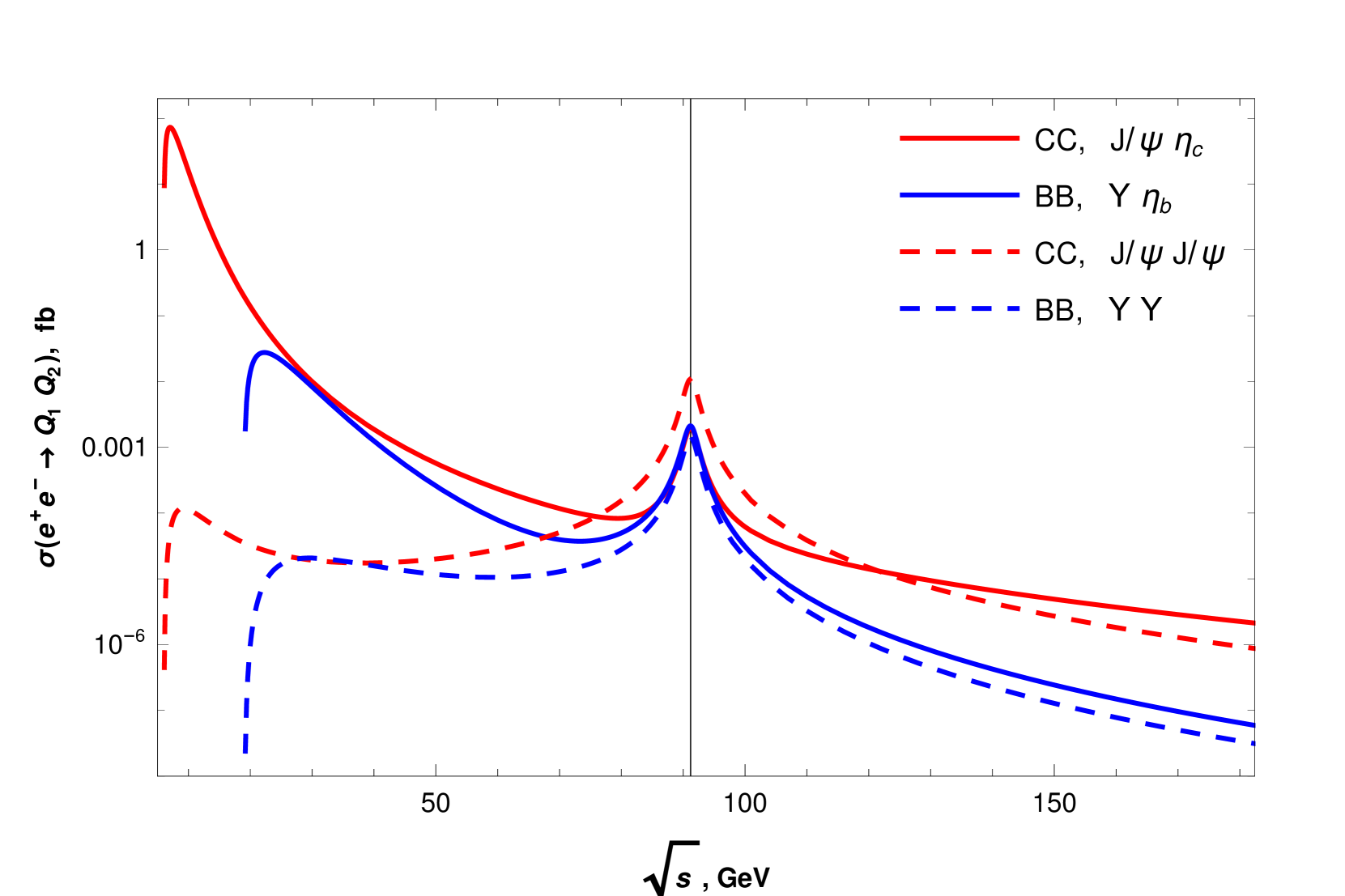
As it is seen in Fig. 1, $J/\psi\,\eta_{c}$ pairs production smaller than $J/\psi\,J/\psi$ only near the $Z$ -pole, while $\Upsilon\,\eta_{b}$ pairs production greater than $\Upsilon\,\Upsilon$ at all investigated energies.
The relative QCD and EW contributions to the total cross sections are shown in Fig. 2. It is worth to note that in the charmonia production the QCD contribution is dominant up to energies of $\sim 25\leavevmode\nobreak\ \text{GeV}$ , while at higher energies the EW contribution dominates. As for the associated bottomonia production, at low energies the QCD mechanism appears to be dominant, while at energies above the $Z$ -boson threshold both contributions are comparable.
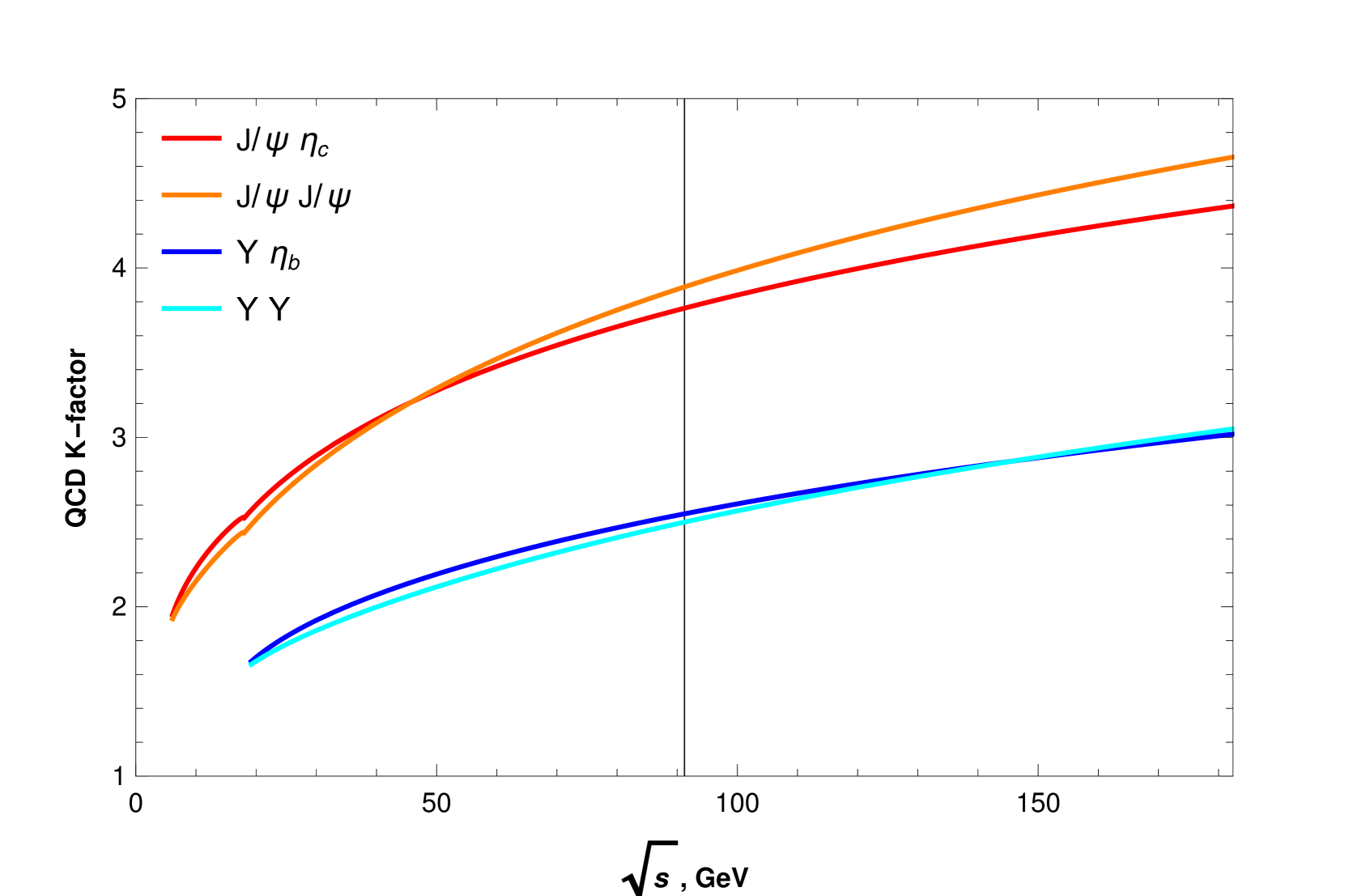
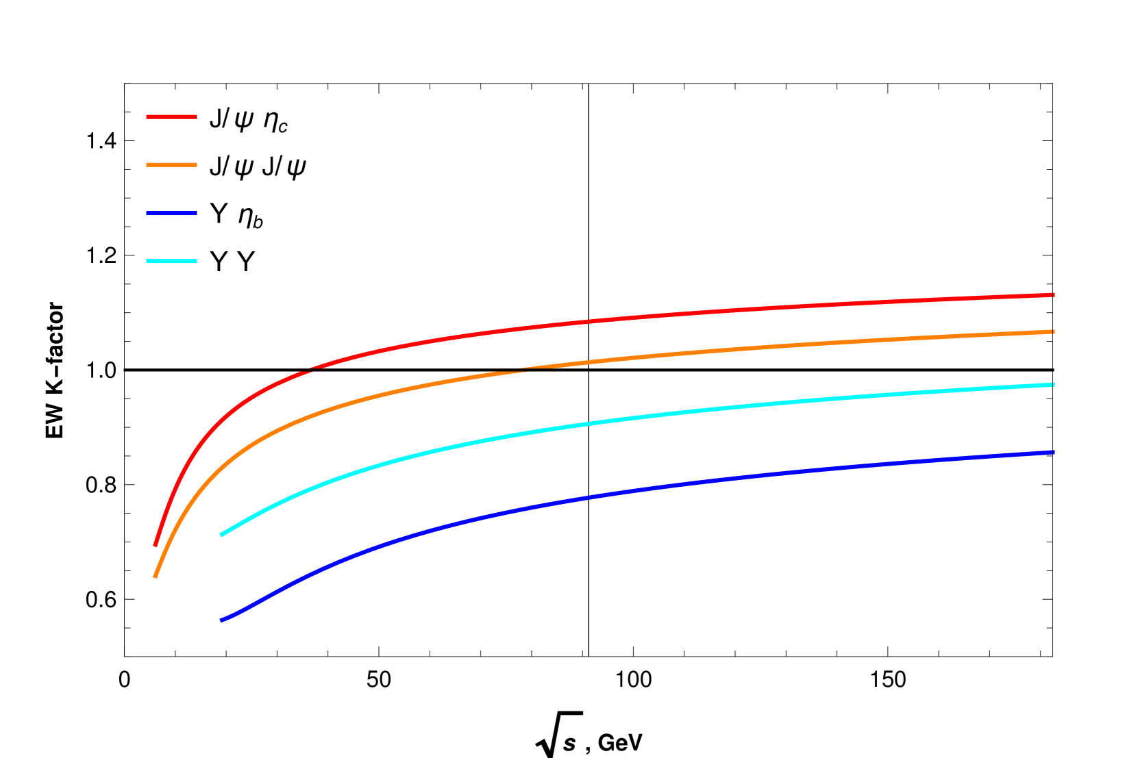
### K-factors
In order to estimate the contribution of NLO corrections to the cross section the K-factors were numerically calculated for each of the production mechanisms.
The K-factors dependencies on interaction energy are shown in Fig. 3 and Fig. 4. All K-factors increase with energy as expected from (4) and (5). The K-factors for the QCD mechanism are consimilar for PV and VV pairs production, whereas K-factors for the EW mechanism are sufficiently depend on quarkonia quantum numbers. The NLO corrections to QCD mechanism contribute positively to the cross section at all investigated energies. The NLO corrections to the EW charmonia production are negative at low energies and positive at high energies. The NLO corrections to the EW bottomonia production are negative at all energies.
The obtained results highlight the significance of NLO corrections to the both discussed mechanisms.
## 4 Conclusions
The exclusive production of charmonia and bottomonia pairs ( $J/\psi\,\eta_{c}$ , $J/\psi\,J/\psi$ , $\Upsilon\,\eta_{b}$ and $\Upsilon\,\Upsilon$ ) in a single boson $e^{+}e^{-}$ annihilation has been investigated at interaction energies from the production threshold to $2M_{Z}$ within the QCD NLO accuracy.
It has been shown that the both studied mechanisms, namely QCD and EW ones, significantly contribute to the cross section in a wide energy range. Analytical expressions for QCD and EW amplitudes and cross sections have been obtained and numerical results for cross sections have been presented. Also, the relative contributions of production mechanisms to the total cross section have been analysed. We believe that the presented results may be of considerable interest for experiments at future $e^{+}e^{-}$ colliders.
Authors are grateful to the organizing committee of ICPPA2022 for the opportunity to make this report. This study was conducted within the scientific program of the National Center for Physics and Mathematics, section #5 „Particle Physics and Cosmology“. Stage 2023-2025. I. Belov acknowledges the support from „BASIS“ Foundation, grant No. 20-2-2-2-1.
## References
- Abe et al. (2004) K. Abe, H. Aihara, Y. Asano, et al., Phys. Rev. D 70, 071102 (2004). https://doi.org/10.1103/PhysRevD.70.071102
- Aubert et al. (2005) B. Aubert, R. Barate, D. Boutigny, et al., Phys. Rev. D 72, 031101 (2005). https://doi.org/10.1103/PhysRevD.72.031101
- Braaten and Lee (2003) E. Braaten, and J. Lee, Phys. Rev. D 67, 054007, (2003). https://doi.org/10.1103/PhysRevD.67.054007 Erratum Phys. Rev. D 72, 099901 (2005). https://doi.org/10.1103/PhysRevD.72.099901
- Dong et al. (2012) H.-R. Dong, F. Feng, and Y. Jia, Phys. Rev. D 85, 114018 (2012). https://doi.org/10.1103/PhysRevD.85.114018
- Li and Wang (2014) X.-H. Li, and J.-X. Wang, Chin. Phys. C 38, 043101 (2014). https://doi.org/10.1088/1674-1137/38/4/043101
- Feng et al. (2019) F. Feng, Y. Jia, Z. Mo, W.-L. Sang, and J.-Y. Zhang, Next-to-next-to-leading-order QCD corrections to $e^{+}e^{-}\to J/\psi+\eta_{c}$ at $B$ factories. ArXiv, https://arxiv.org/abs/1901.08447, Accessed November 25, 2022. https://doi.org/10.48550/arXiv.1901.08447
- Zhang et al. (2006) Y.-J. Zhang, Y.-J. Gao, and K.-T. Chao, Phys. Rev. Lett. 96, 092001 (2006). https://doi.org/10.1103/PhysRevLett.96.092001
- Gong and Wang (2008) B. Gong, and J.-X. Wang, Phys. Rev. D 77, 054028 (2008). https://doi.org/10.1103/PhysRevD.77.054028
- Bondar and Chernyak (2005) A.E. Bondar, and V.L. Chernyak, Phys. Lett. B 612, 215-222 (2005). https://doi.org/10.1016/j.physletb.2005.03.021
- Braguta et al. (2005) V.V. Braguta, A.K. Likhoded, and A.V. Luchinsky, Phys. Rev. D 72, 074019 (2005). https://doi.org/10.1103/PhysRevD.72.074019
- Berezhnoy and Likhoded (2007) A.V. Berezhnoy, and A.K. Likhoded, Phys. Atom. Nucl. 70, 478-484 (2007). https://doi.org/10.1134/S1063778807030052
- Braguta et al. (2006) V.V. Braguta, A.K. Likhoded, and A.V. Luchinsky, Phys. Lett. B 635, 299-304 (2006). https://doi.org/10.1016/j.physletb.2006.03.005
- Bodwin et al. (2006) G.T. Bodwin, D. Kang, and J. Lee, Phys. Rev. D 74, 114028 (2006). https://doi.org/10.1103/PhysRevD.74.114028
- Ebert and Martynenko (2006) D. Ebert, and A.P. Martynenko, Phys. Rev. D 74, 054008 (2006). https://doi.org/10.1103/PhysRevD.74.054008
- Berezhnoy (2008) A.V. Berezhnoy, Phys. Atom. Nucl. 71, 1803-1806 (2008). https://doi.org/10.1134/S1063778808100141
- Ebert et al. (2009) D. Ebert, R.N. Faustov, V.O. Galkin, and A.P. Martynenko, Phys. Lett. B 672, 264-269 (2009). https://doi.org/10.1016/j.physletb.2009.01.029
- Braguta et al. (2008) V.V. Braguta, A.K. Likhoded, and A.V. Luchinsky, Phys. Rev. D 78, 074032 (2008). https://doi.org/10.1103/PhysRevD.78.074032
- Braguta (2009) V.V. Braguta, Phys. Rev. D 79, 074018 (2009). https://doi.org/10.1103/PhysRevD.79.074018
- Sun et al. (2010) Y.-J.Sun, X.-G. Wu, F. Zuo, and T. Huang, Eur. Phys. J. C 67, 117-123 (2010). https://doi.org/10.1140/epjc/s10052-010-1280-z
- Braguta et al. (2012) V.V. Braguta, A.K. Likhoded, and A.V. Luchinsky, Phys. Atom. Nucl. 75, 97-108 (2012). https://doi.org/10.1134/S1063778812010036
- Sun et al. (2018) Z. Sun, X.G. Wu, Y. Ma, and S.J. Brodsky, Phys. Rev. D 98, 094001 (2018). https://doi.org/10.1103/PhysRevD.98.094001
- Aaij et al. (2020) LHCb collaboration, Sci. Bull. 65, 1983-1993 (2020). https://doi.org/10.1016/j.scib.2020.08.032
- Koratzinos (2016) M. Koratzinos, Nucl. Part. Phys. Proc. 273-275, 2326-2328 (2016). https://doi.org/10.1016/j.nuclphysbps.2015.09.380
- Desch et al. (2019) K. Desch, A. Lankford , K. Mazumdar, et al., Recommendations on ILC Project Implementation. OSTI.GOV, https://www.osti.gov/biblio/1833577, Accessed September 25, 2019. https://doi.org/10.2172/1833577
- Abada (2019) A. Abada, M. Abbrescia, S.S. AbdusSalam, et al., Eur. Phys. J. C. 79, 474 (2019). https://doi.org/10.1140/epjc/s10052-019-6904-3
- Sirunyan et al. (2019) The CMS Collaboration, Phys. Lett. B 797, 134811 (2019). https://doi.org/10.1016/j.physletb.2019.134811
- Berezhnoy et al. (2017) A.V. Berezhnoy, A.K. Likhoded, A.I. Onishchenko, and S.V. Poslavsky, Nucl. Phys. B 915, 224-242 (2017). https://doi.org/10.1016/j.nuclphysb.2016.12.013
- Berezhnoy et al. (2021) A.V. Berezhnoy, I.N. Belov, S.V. Poslavsky, and Likhoded, A.K., Phys. Rev. D 104, 034029 (2021). https://doi.org/10.1103/PhysRevD.104.034029
- Lesh (2021) I.N. Belov , A.V. Berezhnoy, and E.A. Leshchenko, Symmetry 13(7), 1262 (2021). https://doi.org/10.3390/sym13071262
- Bodwin et al. (1995) G.T. Bodwin, E. Braaten, and G.P. Lepage, Phys. Rev. D 51, 1125-1171 (1995). https://doi.org/10.1103/PhysRevD.51.1125 Erratum Phys. Rev. D 55, 5853 (1997). https://doi.org/10.1103/PhysRevD.55.5853
- Hahn (2001) T. Hahn, Comput. Phys. Commun. 140, 418-431 (2001). https://doi.org/10.1016/S0010-4655(01)00290-9
- Shtabovenko et al. (2020) V. Shtabovenko, R. Mertig, and F. Orellana, Comput. Phys. Commun. 256, 107478 (2020). https://doi.org/10.1016/j.cpc.2020.107478
- Feng (2012) F. Feng, Comput. Phys. Commun. 183, 2158-2164 (2012). https://doi.org/10.1016/j.cpc.2012.03.025
- Smirnov (2008) A.V. Smirnov, JHEP 10, 107 (2008). https://doi.org/10.1088/1126-6708/2008/10/107
- Patel (2017) H.H. Patel, Comput. Phys. Commun. 218, 66-70 (2017). https://doi.org/10.1016/j.cpc.2017.04.015
5mm
<details>
<summary>x1.png Details</summary>
### Visual Description
\n
## Chart: Cross Section vs. Center of Mass Energy
### Overview
The image presents a chart depicting the cross section (σ) of electron-positron (e⁺e⁻) collisions as a function of the center of mass energy (√s). Four different collision scenarios are plotted, each represented by a distinct line style and color. The y-axis is on a logarithmic scale.
### Components/Axes
* **X-axis:** √s, GeV (Center of Mass Energy in GeV) - ranges from approximately 0 to 180 GeV.
* **Y-axis:** σ(e⁺e⁻ → Q₁Q₂, fb (Cross Section in femtobarns) - logarithmic scale, ranging from approximately 10⁻⁶ to 1.2 fb.
* **Legend:** Located in the top-right corner.
* Red Solid Line: CC, J/ψ ηc
* Blue Solid Line: BB, γ ηb
* Red Dashed Line: CC, J/ψ J/ψ
* Blue Dashed Line: BB, γ γ
### Detailed Analysis
The chart displays four curves representing different particle production scenarios.
* **Red Solid Line (CC, J/ψ ηc):** This line starts at approximately 1.2 fb at √s ≈ 0 GeV, rapidly decreasing to approximately 0.01 fb at √s ≈ 60 GeV. It then continues to decrease, leveling off around 10⁻⁵ fb at √s ≈ 180 GeV. There is a sharp peak at the beginning of the curve.
* **Blue Solid Line (BB, γ ηb):** This line exhibits a peak around √s ≈ 10 GeV, reaching a maximum cross section of approximately 0.003 fb. It then decreases to approximately 10⁻⁶ fb at √s ≈ 180 GeV.
* **Red Dashed Line (CC, J/ψ J/ψ):** This line starts at approximately 10⁻⁵ fb at √s ≈ 0 GeV, rises to a peak of approximately 0.0015 fb at √s ≈ 95 GeV, and then decreases to approximately 5x10⁻⁶ fb at √s ≈ 180 GeV.
* **Blue Dashed Line (BB, γ γ):** This line starts at approximately 10⁻⁵ fb at √s ≈ 0 GeV, rises to a peak of approximately 0.001 fb at √s ≈ 90 GeV, and then decreases to approximately 2x10⁻⁶ fb at √s ≈ 180 GeV.
### Key Observations
* The CC, J/ψ ηc channel has the highest cross section at low energies.
* The BB, γ ηb channel exhibits a peak at lower energies compared to the other channels.
* The CC, J/ψ J/ψ and BB, γ γ channels show similar behavior, with peaks around √s ≈ 90-95 GeV.
* All channels exhibit decreasing cross sections at higher energies.
* The y-axis is logarithmic, emphasizing the differences in cross sections across different energy ranges.
### Interpretation
This chart likely represents theoretical predictions or experimental measurements of the cross sections for producing various particle combinations (J/ψ ηc, γ ηb, J/ψ J/ψ, γ γ) in electron-positron collisions. The peaks in the curves correspond to resonance energies where the production of these particles is enhanced. The decreasing cross sections at higher energies are consistent with the expected behavior of quantum field theory, where the probability of particle production decreases with increasing energy.
The differences in the shapes and magnitudes of the curves provide insights into the underlying dynamics of the interactions. For example, the higher cross section for the CC, J/ψ ηc channel at low energies suggests a stronger coupling or a more favorable phase space for this process. The peaks around 90-95 GeV for the CC, J/ψ J/ψ and BB, γ γ channels indicate the presence of resonances at those energies, potentially corresponding to new particles or excited states.
The logarithmic scale on the y-axis is crucial for visualizing the wide range of cross sections involved. Without it, the lower cross sections would be difficult to discern. The chart is a valuable tool for understanding the production mechanisms of these particles and for testing the predictions of theoretical models.
</details>
normal
Figure 1: The total cross sections dependence on the collision energy for the double charmonia and the double bottomonia production.
5mm $\begin{array}[]{cc}\includegraphics[page=1,width=216.81pt]{pictures/sigma/Fig2 .pdf}&\includegraphics[page=2,width=216.81pt]{pictures/sigma/Fig2.pdf}\\ (a)\leavevmode\nobreak\ J/\psi\,\eta_{c}&(b)\leavevmode\nobreak\ J/\psi\,J/ \psi\\ \includegraphics[page=3,width=216.81pt]{pictures/sigma/Fig2.pdf}& \includegraphics[page=4,width=216.81pt]{pictures/sigma/Fig2.pdf}\\ (c)\leavevmode\nobreak\ \Upsilon\,\eta_{b}&(d)\leavevmode\nobreak\ \Upsilon\, \Upsilon\end{array}$ normal
Figure 2: Relative contributions of different different mechanisms to the total cross section values as a function of collision energy: the QCD mechanism (red), the EW mechanism (blue), the interference of QCD and EW production mechanisms (green).
5mm
<details>
<summary>x6.png Details</summary>
### Visual Description
\n
## Chart: QCD K-factor vs. √s
### Overview
The image presents a line chart illustrating the relationship between the QCD K-factor and the square root of the center-of-mass energy (√s, in GeV). Four different particle combinations are represented by distinct colored lines, showing how the K-factor changes with increasing energy.
### Components/Axes
* **X-axis:** √s (GeV), ranging from 0 to approximately 160 GeV. The axis is labeled "√s , GeV".
* **Y-axis:** QCD K-factor, ranging from 1 to 5. The axis is labeled "QCD K-factor".
* **Legend (Top-Right):**
* Red Line: J/ψ ηc
* Orange Line: J/ψ J/ψ
* Dark Orange Line: γ ηb
* Blue Line: γ γ
### Detailed Analysis
The chart displays four curves, each representing a different particle combination and its corresponding K-factor as a function of √s.
* **J/ψ ηc (Red Line):** This line starts at approximately 2.1 at √s = 0 GeV and increases with a decreasing slope, reaching approximately 4.4 at √s = 160 GeV. The curve exhibits a significant initial rise, then plateaus.
* **J/ψ J/ψ (Orange Line):** This line begins at approximately 3.4 at √s = 0 GeV and increases with a relatively constant, but shallow slope, reaching approximately 4.1 at √s = 160 GeV.
* **γ ηb (Dark Orange Line):** This line starts at approximately 2.4 at √s = 0 GeV and increases with a moderate slope, reaching approximately 3.6 at √s = 160 GeV.
* **γ γ (Blue Line):** This line starts at approximately 1.9 at √s = 0 GeV and increases with a moderate slope, reaching approximately 2.8 at √s = 160 GeV. This line exhibits the lowest K-factor values across the entire energy range.
### Key Observations
* The K-factor generally increases with increasing √s for all particle combinations.
* The J/ψ J/ψ combination consistently exhibits the highest K-factor values.
* The γ γ combination consistently exhibits the lowest K-factor values.
* The rate of increase in K-factor appears to diminish at higher √s values for all combinations.
### Interpretation
This chart likely represents theoretical predictions or experimental measurements of the QCD K-factor for different particle production processes. The K-factor is a multiplicative correction applied to leading-order calculations in perturbative quantum chromodynamics (QCD) to account for higher-order corrections. A higher K-factor indicates that higher-order corrections are more significant.
The differences in K-factor values between the different particle combinations suggest that the higher-order QCD corrections are process-dependent. The J/ψ J/ψ channel having the highest K-factor implies that higher-order corrections are particularly important for this process. Conversely, the γ γ channel having the lowest K-factor suggests that leading-order calculations may be sufficient for this process.
The diminishing rate of increase in K-factor at higher √s values could indicate that the perturbative expansion is becoming less reliable at higher energies, or that non-perturbative effects are becoming more important. The chart provides valuable information for understanding the accuracy of QCD predictions and for guiding experimental searches for these particles.
</details>
normal
Figure 3: The total K-factor dependence on the collision energy in case of QCD production.
5mm
<details>
<summary>x7.png Details</summary>
### Visual Description
\n
## Chart: EW K-factor vs. √s
### Overview
The image presents a line chart illustrating the Electroweak (EW) K-factor as a function of the square root of the center-of-mass energy (√s) in GeV. The chart displays four different curves, each representing a specific particle interaction.
### Components/Axes
* **X-axis:** √s, GeV (Square root of the center-of-mass energy in GeV). Scale ranges from 0 to 180, with tick marks at 0, 50, 100, 150.
* **Y-axis:** EW K-factor. Scale ranges from 0.6 to 1.4, with tick marks at 0.6, 0.8, 1.0, 1.2, 1.4.
* **Legend:** Located in the top-right corner. Contains the following labels and corresponding colors:
* J/ψ ηc (Red)
* J/ψ J/ψ (Orange)
* γ ηb (Blue)
* γ γ (Cyan)
### Detailed Analysis
The chart shows four curves, each representing the EW K-factor for a different particle interaction as a function of √s.
* **J/ψ ηc (Red):** This line starts at approximately 1.35 at √s = 0 GeV and decreases rapidly to around 0.95 at √s = 20 GeV. It then plateaus, approaching a value of approximately 1.05 at √s = 150 GeV. The line exhibits a strong initial decline followed by stabilization.
* **J/ψ J/ψ (Orange):** This line begins at approximately 1.1 at √s = 0 GeV and decreases to around 0.9 at √s = 20 GeV. It then gradually increases, reaching approximately 1.0 at √s = 100 GeV and remaining relatively constant at around 1.02 at √s = 150 GeV. The line shows a moderate initial decline and a subsequent slow increase.
* **γ ηb (Blue):** This line starts at approximately 0.65 at √s = 0 GeV and increases steadily, reaching approximately 0.85 at √s = 100 GeV and continuing to rise to around 0.9 at √s = 150 GeV. The line demonstrates a consistent upward trend.
* **γ γ (Cyan):** This line begins at approximately 0.8 at √s = 0 GeV and increases slowly, reaching approximately 0.9 at √s = 50 GeV and remaining relatively constant at around 0.92 at √s = 150 GeV. The line shows a gradual increase followed by stabilization.
### Key Observations
* All four curves converge towards a K-factor of approximately 1.0 as √s increases.
* The J/ψ ηc interaction has the highest K-factor at low energies (√s < 50 GeV).
* The γ ηb interaction has the lowest K-factor at low energies (√s < 50 GeV).
* The γ γ interaction exhibits the most stable K-factor across the entire energy range.
### Interpretation
The chart illustrates how electroweak corrections (represented by the K-factor) affect different particle interactions at varying energy scales. The K-factor quantifies the ratio of the full electroweak calculation to the leading-order approximation. As the center-of-mass energy increases, the electroweak corrections become less significant, and the K-factors approach 1.0 for all interactions. This suggests that at high energies, the electroweak effects are less pronounced.
The differences in K-factor values between the interactions indicate that electroweak corrections are more important for some processes than others. The J/ψ ηc interaction, for example, experiences a more substantial correction at lower energies compared to the γ γ interaction. This could be due to the different masses and couplings of the involved particles.
The convergence of the K-factors at high energies is consistent with the expectation that electroweak effects become less important as the energy scale increases, and the interactions become more dominated by strong interactions. The chart provides valuable insights into the energy dependence of electroweak corrections in particle physics.
</details>
normal
Figure 4: The total K-factor dependence on the collision energy in case of EW production.
0mm flushleft $m_{c}$ = 1.5 GeV $m_{b}$ = 4.7 GeV $M_{Z}$ = 91.2 GeV $\Gamma_{Z}$ = 2.5 GeV $\langle O\rangle_{J/\psi}=\langle O\rangle_{\eta_{c}}=0.523\mbox{ GeV}^{3}$ $\langle O\rangle_{\Upsilon}=\langle O\rangle_{\eta_{b}}=2.797\mbox{ GeV}^{3}$ $\sin^{2}\theta_{w}$ = 0.23
Table 1: The cross section values in fb units at different collision energies.
0mm flushleft E, GeV 15 20 30 50 90 180 $\leavevmode\nobreak\ J/\psi\,\eta_{c}\leavevmode\nobreak\$ $1.15\cdot 10^{0}$ $1.38\cdot 10^{-1}$ $9.96\cdot 10^{-3}$ $5.71\cdot 10^{-4}$ $1.04\cdot 10^{-3}$ $2.25\cdot 10^{-6}$ $\leavevmode\nobreak\ J/\psi\,J/\psi\leavevmode\nobreak\$ $5.67\cdot 10^{-5}$ $3.23\cdot 10^{-5}$ $1.92\cdot 10^{-5}$ $2.00\cdot 10^{-5}$ $5.70\cdot 10^{-3}$ $9.37\cdot 10^{-7}$ $\leavevmode\nobreak\ \Upsilon\,\eta_{b}\leavevmode\nobreak\$ $-$ $1.40\cdot 10^{-2}$ $8.30\cdot 10^{-3}$ $2.59\cdot 10^{-4}$ $1.15\cdot 10^{-3}$ $6.47\cdot 10^{-8}$ $\leavevmode\nobreak\ \Upsilon\,\Upsilon\leavevmode\nobreak\$ $-$ $9.84\cdot 10^{-7}$ $2.07\cdot 10^{-5}$ $1.17\cdot 10^{-5}$ $7.65\cdot 10^{-4}$ $3.41\cdot 10^{-8}$
Table 2: The cross section values in fb units at different collision energies.