2303.14061v4

## Learning Reward Machines in Cooperative Multi-Agent Tasks Leo Ardon Imperial College London ## ABSTRACT This paper presents a novel approach to Multi-Agent Reinforcement Learning (MARL) that combines cooperative task decomposition with the learning of reward machines (RMs) encoding the structure of the sub-tasks. The proposed method helps deal with the non-Markovian nature of the rewards in partially observable environments and improves the interpretability of the learnt policies required to complete the cooperative task. The RMs associated with each sub-task are learnt in a decentralised manner and then used to guide the behaviour of each agent. By doing so, the complexity of a cooperative multi-agent problem is reduced, allowing for more effective learning. The results suggest that our approach is a promising direction for future research in MARL, especially in complex environments with large state spaces and multiple agents. ## KEYWORDS Reinforcement Learning; Multi-agent; Reward Machine; NeuroSymbolic ## ACMReference Format: Leo Ardon, Daniel Furelos-Blanco, and Alessandra Russo. 2023. Learning Reward Machines in Cooperative Multi-Agent Tasks. In Proc. of the 22nd International Conference on Autonomous Agents and Multiagent Systems (AAMAS 2023), London, United Kingdom, May 29 - June 2, 2023 , IFAAMAS, 8 pages. ## 1 INTRODUCTION With impressive advances in the past decade, the Reinforcement Learning (RL) [18] paradigm appears as a promising avenue in the quest to have machines learn autonomously how to achieve a goal. Originally evaluated in the context of a single agent interacting with the rest of the world, researchers have since then extended the approach to the multi-agent setting (MARL), where multiple autonomous entities learn in the same environment. Multiple agents learning concurrently brings a set of challenges, such as partial observability, non-stationarity, and scalability; however, this setting is more realistic. Like in many real-life scenarios, the actions of one individual often affect the way others act and should therefore be considered in the learning process. A sub-field of MARL called Cooperative Multi-Agent Reinforcement Learning (CMARL) focuses on learning policies for multiple agents that must coordinate their actions to achieve a shared objective. With a 'divide and conquer' strategy, complex problems can thus be decomposed into smaller and simpler ones assigned to different agents acting in parallel in the environment. The problem of learning an optimal sequence of actions now also includes the need to strategically divide the task among agents that must learn Proc. of the 22nd International Conference on Autonomous Agents and Multiagent Systems (AAMAS 2023), A. Ricci, W. Yeoh, N. Agmon, B. An (eds.), May 29 - June 2, 2023, London, United Kingdom . © 2023 International Foundation for Autonomous Agents and Multiagent Systems (www.ifaamas.org). All rights reserved. Daniel Furelos-Blanco Imperial College London Alessandra Russo Imperial College London to coordinate and communicate in order to find the optimal way to accomplish the goal. An emergent field of research in the RL community exploits finite-state machines to encode the structure of the reward function; ergo, the structure of the task at hand. This new construct, introduced by Toro Icarte et al. [19] and called reward machine (RM), can model non-Markovian reward and provides a symbolic interpretation of the stages required to complete a task. While the structure of the task is sometimes known in advance, it is rarely true in practice. Learning the RM has thus been the object of several works in recent years [3, 9, 10, 13, 21, 22] as a way to reduce the human input. In the multi-agent settings, however, the challenges highlighted before make the learning of the RM encoding the global task particularly difficult. Instead, it is more efficient to learn the RMs of smaller tasks obtained from an appropriate task decomposition. The 'global' RM can later be reconstructed with a parallel composition of the RM of the sub-tasks. Inspired by the work of Neary et al. [16] using RMs to decompose and distribute a global task to a team of collaborative agents, we propose a method combining task decomposition with autonomous learning of the RMs. Our approach offers a more scalable and interpretable way to learn the structure of a complex task involving collaboration among multiple agents. We present an algorithm that learns in parallel the RMs associated with the sub-task of each agent and their associated RL policies whilst guaranteeing that their executions achieve the global cooperative task. We experimentally show that with our method a team of agents is able to learn how to solve a collaborative task in two different environments. ## 2 BACKGROUND This section gives a summary of the relevant background to make the paper self-contained. Given a finite set X , Δ (X) denotes the probability simplex over X , X ∗ denotes (possibly empty) sequences of elements from X , and X + is a non-empty sequence. The symbols ⊥ and ⊤ denote false and true, respectively. ## 2.1 Reinforcement Learning Weconsider 𝑇 -episodic labeled Markovdecision processes (MDPs) [22], characterized by a tuple ⟨S , 𝑠 𝐼 , A , 𝑝, 𝑟, 𝑇 , 𝛾, P , 𝑙 ⟩ consisting of a set of states S , an initial state 𝑠 𝐼 ∈ S , a set of actions A , a transition function 𝑝 : S × A → Δ (S) , a not necessarily Markovian reward function 𝑟 : (S ×A) + ×S → R , the time horizon 𝑇 of each episode, a discount factor 𝛾 ∈ [ 0 , 1 ) , a finite set of propositions P , and a labeling function 𝑙 : S × S → 2 P . A (state-action) history ℎ 𝑡 = ⟨ 𝑠 0 , 𝑎 0 , . . . , 𝑠 𝑡 ⟩ ∈ (S × A) ∗ × S is mapped into a label trace (or trace) 𝜆 𝑡 = ⟨ 𝑙 ( 𝑠 0 , 𝑠 1 ) , . . . , 𝑙 ( 𝑠 𝑡 -1 , 𝑠 𝑡 )⟩ ∈ ( 2 P ) + by applying the labeling function to each state transition in ℎ 𝑡 . We assume that the reward function can be written in terms of a label trace, i.e. formally 𝑟 ( ℎ 𝑡 + 1 ) = 𝑟 ( 𝜆 𝑡 + 1 , 𝑠 𝑡 + 1 ) . The goal is to find an optimal policy 𝜋 : ( 2 P ) + × S → A , mapping (traces-states) to actions, in order to maximize the expected cumulative discounted reward 𝑅 𝑡 = E 𝜋 h ˝ 𝑇 𝑘 = 𝑡 𝛾 𝑘 -𝑡 𝑟 ( 𝜆 𝑘 + 1 , 𝑠 𝑘 + 1 ) i . At time 𝑡 , the agent keeps a trace 𝜆 𝑡 ∈ ( 2 P ) + , and observes state 𝑠 𝑡 ∈ S . The agent chooses the action to execute with its policy 𝑎 = 𝜋 ( 𝜆 𝑡 , 𝑠 𝑡 ) ∈ A , and the environment transitions to state 𝑠 𝑡 + 1 ∼ 𝑝 (· | 𝑠 𝑡 , 𝑎 𝑡 ) . As a result, the agent observes a new state 𝑠 𝑡 + 1 and a new label L 𝑡 + 1 = 𝑙 ( 𝑠 𝑡 , 𝑠 𝑡 + 1 ) , and gets the reward 𝑟 𝑡 + 1 = 𝑟 ( 𝜆 𝑡 + 1 , 𝑠 𝑡 + 1 ) . The trace 𝜆 𝑡 + 1 = 𝜆 𝑡 ⊕ L 𝑡 + 1 is updated with the new label. In this work, we focus on the goal-conditioned RL problem [14] where the agent's task is to reach a goal state as rapidly as possible. We thus distinguish between two types of traces: goal traces and incomplete traces. A trace 𝜆 𝑡 is said to be a goal trace if the task's goal has been achieved before 𝑡 otherwise we say that the trace is incomplete . Formally, the MDP includes a termination function 𝜏 : ( 2 P ) + × S → {⊥ , ⊤} indicating that the trace 𝜆 𝑡 at time 𝑡 is an incomplete trace if 𝜏 ( 𝜆 𝑡 , 𝑠 𝑡 ) = ⊥ or a goal trace if 𝜏 ( 𝜆 𝑡 , 𝑠 𝑡 ) = ⊤ . We assume the reward is 1 for goal traces and 0 otherwise. For ease of notation, we will refer to a goal trace as 𝜆 ⊤ 𝑡 and an incomplete trace as 𝜆 ⊥ 𝑡 . Note that we assume the agent-environment interaction stops when the task's goal is achieved. This is without loss of generality as it is equivalent to having a final absorbing state with a null reward associated and no label returned by the labeling function 𝑙 . The single-agent framework above can be extended to the collaborative multi-agent setting as a Markov game. A cooperative Markov game of 𝑁 agents is a tuple G = ⟨ 𝑁, S , 𝒔 𝐼 , A , 𝑝, 𝑟, 𝜏, 𝑇 , 𝛾, P , 𝑙 ⟩ , where S = S 1 × · · · × S 𝑁 is the set of joint states, 𝒔 𝐼 ∈ S is a joint initial state, A = A 1 ×· · · × A 𝑁 is the set of joint actions, 𝑝 : S × A → Δ ( S ) is a joint transition function, 𝑟 : ( S × A ) + × S → R is the collective reward function, 𝜏 : ( 2 P ) + × S → {⊥ , ⊤} is the collective termination function, and 𝑙 : S × S → 2 P is an event labeling function. 𝑇 , 𝛾 , and P are defined as for MDPs. Like Neary et al. [16], we assume each agent 𝐴 𝑖 's dynamics are independently governed by local transition functions 𝑝 𝑖 : S 𝑖 ×A 𝑖 → Δ (S 𝑖 ) , hence the joint transition function is 𝑝 ( 𝒔 ′ | 𝒔 , 𝒂 ) = Π 𝑁 𝑖 = 1 𝑝 ( 𝑠 ′ 𝑖 | 𝑠 𝑖 , 𝑎 𝑖 ) for all 𝒔 , 𝒔 ′ ∈ S and 𝒂 ∈ A . The objective is to find a team policy 𝜋 : ( 2 P ) + × S → A mapping pairs of traces and joint states to joint actions that maximizes the expected cumulative collective reward. 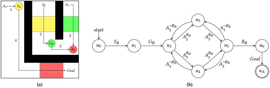Example 2.1. We use the ThreeButtons task [16], illustrated in Figure 1a, as a running example. The task consists of three agents ( 𝐴 1 , 𝐴 2 , and 𝐴 3 ) that must cooperate for agent 𝐴 1 to get to the 𝐺𝑜𝑎𝑙 position. To achieve this, agents must open doors that prevent other agents from progressing by pushing buttons 𝑌 𝐵 , 𝐺 𝐵 , and 𝑅 𝐵 . The button of a given color opens the door of the same color and, two agents are required to push 𝑅 𝐵 at once hence involving synchronization. Once a door has been opened, it remains open until the end of the episode. The order in which high-level actions must be performed is shown in the figure: (1) 𝐴 1 pushes 𝑌 𝐵 , (2) 𝐴 2 pushes 𝐺 𝐵 , (3) 𝐴 2 and 𝐴 3 push 𝑅 𝐵 , and (4) 𝐴 1 reaches 𝐺𝑜𝑎𝑙 . We can formulate this problem using the RL framework by defining a shared reward function returning 1 when the 𝐺𝑜𝑎𝑙 position is reached. States solely consist of the position of the agents in the environment. The proposition set in this task is P = { 𝑅 𝐵 , 𝑌 𝐵 , 𝐺 𝐵 , 𝐴 ¬ 𝑅 𝐵 2 , 𝐴 𝑅 𝐵 2 , 𝐴 ¬ 𝑅 𝐵 3 , 𝐴 𝑅 𝐵 3 , 𝐺𝑜𝑎𝑙 } , where (i) 𝑅 𝐵 , 𝑌 𝐵 and 𝐺 𝐵 indicate that the red, yellow and green buttons have been pushed respectively, (ii) 𝐴 𝑅 𝐵 𝑖 (resp. 𝐴 ¬ 𝑅 𝐵 𝑖 ), where 𝑖 ∈ { 2 , 3 } , indicates that agent 𝐴 𝑖 is (resp. has stopped) pushing the red button 𝑅 𝐵 , and (iii) 𝐺𝑜𝑎𝑙 indicates that the goal position has been reached. A minimal goal trace is ⟨{} , { 𝑌 𝐵 } , { 𝐺 𝐵 } , { 𝐴 𝑅 𝐵 2 } , { 𝐴 𝑅 𝐵 3 } , { 𝑅 𝐵 } , { 𝐺𝑜𝑎𝑙 }⟩ . ## 2.2 Reward Machines We here introduce reward machines, the formalism we use to express decomposable (multi-agent) tasks. ## 2.2.1 Definitions. A reward machine (RM) [19, 20] is a finite-state machine that represents the reward function of an RL task. Formally, an RM is a tuple 𝑀 = ⟨U , P , 𝑢 0 , 𝑢 𝐴 , 𝛿 𝑢 , 𝛿 𝑟 ⟩ where U is a set of states; P is a set of propositions; 𝑢 0 ∈ U is the initial state; 𝑢 𝐴 ∈ U is the final state; 𝛿 𝑢 : U × 2 P → U is a state-transition function such that 𝛿 𝑢 ( 𝑢, L) is the state that results from observing label L ∈ 2 P in state 𝑢 ∈ U ; and 𝛿 𝑟 : U×U → R is a reward-transition function such that 𝛿 𝑟 ( 𝑢,𝑢 ′ ) is the reward obtained for transitioning from state 𝑢 ∈ U to 𝑢 ′ ∈ U . We assume that (i) there are no outgoing transitions from 𝑢 𝐴 , and (ii) 𝛿 𝑟 ( 𝑢,𝑢 ′ ) = 1 if 𝑢 ′ = 𝑢 𝐴 and 0 otherwise (following the reward assumption in Section 2.1). Given a trace 𝜆 = ⟨L 0 , . . . , L 𝑛 ⟩ , a traversal (or run) is a sequence of RM states ⟨ 𝑣 0 , . . . , 𝑣 𝑛 + 1 ⟩ such that 𝑣 0 = 𝑢 0 , and 𝑣 𝑖 + 1 = 𝛿 𝑢 ( 𝑣 𝑖 , L 𝑖 ) for 𝑖 ∈ [ 1 , 𝑛 ] . Ideally, RMs are such that (i) the cross product S × U of their states with the MDP's make the reward and termination functions Markovian, and (ii) traversals for goal traces end in the final state 𝑢 𝐴 and traversals for incomplete traces do not. Example 2.2. Figure 1b shows an RM for the ThreeButtons task. For simplicity, edges are labeled using the single proposition that triggers the transitions instead of sets. Note that the goal trace introduced in Example 2.1 ends in the final state 𝑢 𝐴 . ## 2.2.2 RL Algorithm. The Q-learning for RMs (QRM) algorithm [19, 20] exploits the task structure modeled through RMs. QRM learns a Q-function 𝑞 𝑢 for each state 𝑢 ∈ U in the RM. Given an experience tuple ⟨ 𝑠, 𝑎, 𝑠 ′ ⟩ , a Q-function 𝑞 𝑢 is updated as follows: <!-- formula-not-decoded --> where 𝑢 ′ = 𝛿 𝑢 ( 𝑢, 𝑙 ( 𝑠, 𝑠 ′ )) . All Q-functions (or a subset of them) are updated at each step using the same experience tuple in a counterfactual manner. In the tabular case, QRM is guaranteed to converge to an optimal policy. ## 2.2.3 Multi-Agent Decomposition. Neary et al. [16] recently proposed to decompose the RM for a multiagent task into several RMs (one per agent) executed in parallel. The task decomposition into individual and independently learnable sub-tasks addresses the problem of non-stationarity inherent in the multi-agent setting. The use of RMs gives the high-level structure of the task each agent must solve. In this setting, each agent 𝐴 𝑖 has its own RM 𝑀 𝑖 , local state space S 𝑖 (e.g., it solely observes its position in the grid), and propositions P 𝑖 such that P = -𝑖 P 𝑖 . Besides, instead of having a single opaque labeling function, each agent 𝐴 𝑖 employs its own labeling function 𝑙 𝑖 : S 𝑖 ×S 𝑖 → 2 P 𝑖 . Each labeling function is assumed to return at most one proposition per Figure 1: Illustration of the ThreeButtons grid (a) and a reward machine modeling the task's structure (b) [16]. <details> <summary>Image 1 Details</summary>  ### Visual Description ## Diagram: State Transition and Grid Layout System ### Overview The image contains two interconnected components: 1. **(a) Grid Layout**: A spatial representation with labeled zones, colored regions, and directional connections. 2. **(b) State Transition Diagram**: A flowchart depicting a process flow with nodes, transitions, and goal states. --- ### Components/Axes #### (a) Grid Layout - **Labels**: - `A1`, `A2`, `A3`: Vertical/horizontal axis labels (left and top edges). - `Y_B`, `G_B`, `R_B`: Node labels within the grid. - `Goal`: Terminal state at the bottom-right. - **Colors**: - Yellow (`A1` zone), Green (`A2` zone), Black (obstacle), Red (`Goal`). - **Connections**: - Dotted lines indicate transitions between nodes (e.g., `Y_B` → `G_B` → `R_B`). - **Spatial Grounding**: - `Y_B` is positioned at the top-left corner. - `Goal` is anchored at the bottom-right. - Obstacles (black) block direct paths between zones. #### (b) State Transition Diagram - **Nodes**: - `u0` (start), `u1`, `u2`, `u3`, `u4`, `u5`, `u6` (goal), `u_A` (alternate goal). - **Transitions**: - Labeled with actions/states: `A2^RB`, `A3^RB`, `A2^RB`, `A3^RB`, `R_B`. - Arrows indicate directionality (e.g., `u2` → `u3` via `A2^RB`). - **Spatial Grounding**: - Nodes form a loop (`u3` → `u4` → `u5` → `u3`). - `u6` (goal) is terminal; `u_A` is an alternate endpoint. --- ### Detailed Analysis #### (a) Grid Layout - **Zones**: - `A1` (yellow): Top-left region, connected to `Y_B`. - `A2` (green): Middle region, connected to `G_B`. - `A3` (black/red): Right-side obstacle/goal region. - **Path Constraints**: - Obstacles (black) force indirect routing (e.g., `Y_B` → `G_B` → `R_B`). - `Goal` is accessible only via `R_B`. #### (b) State Transition Diagram - **Flow Logic**: - Start (`u0`) → `Y_B` → `u1` → `G_B` → `u2`. - From `u2`, transitions branch to `u3`, `u4`, `u5` via `A2^RB`/`A3^RB`. - Loop between `u3`, `u4`, `u5` using `A2^RB`/`A3^RB`. - Exit to `u6` (goal) via `R_B` or `u_A`. - **Key Nodes**: - `u2`: Decision point for branching. - `u5`: Convergence point for loop transitions. --- ### Key Observations 1. **Grid-to-Flow Correlation**: - `Y_B`, `G_B`, `R_B` in the grid map to `u1`, `u2`, `u5` in the flowchart. - Obstacles in the grid (`A3` black) align with constrained transitions in the flowchart. 2. **Redundancy**: - Multiple paths to `u6` (goal) via `R_B` and `u_A`. 3. **Cyclical Behavior**: - Loop between `u3`, `u4`, `u5` suggests iterative processing. --- ### Interpretation This system models a **state-dependent navigation process** where spatial constraints (grid) dictate allowable transitions (flowchart). - **Purpose**: - The grid represents a physical or logical environment with zones and obstacles. - The flowchart abstracts the decision-making process for navigating these zones. - **Notable Patterns**: - The loop (`u3`→`u4`→`u5`) implies repeated evaluation or resource allocation. - Dual goal states (`u6` and `u_A`) suggest contingency planning. - **Anomalies**: - No explicit mechanism to exit the loop (`u3`→`u4`→`u5`) without reaching `u6`/`u_A`. This dual representation bridges spatial reasoning (grid) with algorithmic logic (flowchart), emphasizing path optimization under constraints. 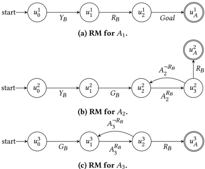</details> Figure 2: RMs for each of the agents in ThreeButtons [16]. <details> <summary>Image 2 Details</summary>  ### Visual Description ## Diagram: Reachability Models (RM) for Agents A1, A2, A3 ### Overview The image presents three distinct Reachability Models (RM) for agents A1, A2, and A3. Each model illustrates a state transition system with nodes representing states (e.g., `u0`, `u1`, `uA`) and edges labeled with transition conditions (e.g., `YB`, `RB`, `GB`, `A2^RB`, `A3^RB`). The diagrams emphasize differences in state connectivity and transition logic between agents. ### Components/Axes - **Nodes**: - Labeled as `u0` (start), `u1`, `u2`, `u3`, and `uA` (goal). - Nodes are enclosed in circles, with `uA` highlighted by a double border in all diagrams. - **Edges**: - Directed arrows represent transitions between states. - Labels on edges include: - `YB` (Yes/No condition?), `RB` (Reachability?), `GB` (Goal condition?), `A2^RB`, `A3^RB` (agent-specific transitions). - **Diagram Structure**: - **Diagram (a)**: Linear path from `start` → `u0` → `u1` → `u2` → `uA` (Goal). - **Diagram (b)**: Path with a loop: `start` → `u0` → `u1` → `u2` → `u3` (via `A2^RB`) → `uA`. - **Diagram (c)**: Path with a loop: `start` → `u0` → `u1` → `u2` (via `A3^RB`) → `u3` → `uA`. ### Detailed Analysis - **Diagram (a) (RM for A1)**: - Simplest structure: Direct linear progression from `u0` to `uA` via `u1` and `u2`. - Edges: `YB` (start→u0), `RB` (u1→u2), `Goal` (u2→uA). - **Diagram (b) (RM for A2)**: - Introduces a loop between `u2` and `u3` via `A2^RB` (u2→u3) and `RB` (u3→uA). - Additional edge `GB` (u1→u2) suggests a goal-related transition. - **Diagram (c) (RM for A3)**: - Loop between `u1` and `u2` via `A3^RB` (u1→u2) and `RB` (u2→u3). - Edge `GB` (u0→u1) indicates a goal-related transition at an earlier stage. ### Key Observations 1. **Agent-Specific Transitions**: - A1 follows a linear path without loops. - A2 and A3 include loops (`A2^RB`, `A3^RB`), implying conditional or iterative behaviors. 2. **Transition Labels**: - `YB`, `RB`, and `GB` appear consistently but with varying roles across diagrams. - `A2^RB` and `A3^RB` suggest agent-specific reachability conditions. 3. **Goal State (`uA`)**: - Always the terminal node, marked distinctly with a double border. ### Interpretation The diagrams model how agents A1, A2, and A3 navigate state spaces to achieve a goal (`uA`). - **A1’s Model**: Represents a straightforward, deterministic path with no branching or loops. - **A2’s Model**: The loop (`A2^RB`) implies a conditional retry or alternative route, possibly for handling failures or optimizing reachability. - **A3’s Model**: The earlier `GB` transition (u0→u1) suggests goal-oriented actions are prioritized early in the process. The use of superscripts (`A2^RB`, `A3^RB`) may denote inverse or specialized reachability conditions unique to each agent. These models could represent decision-making frameworks where agents adapt their strategies based on environmental conditions (e.g., `YB` for yes/no checks, `RB` for reachability constraints). ### Notable Patterns - **Increasing Complexity**: From A1 to A3, the models grow more complex, with added loops and agent-specific transitions. - **Shared Elements**: All diagrams share `YB`, `RB`, and `GB`, indicating common transition types across agents. - **Goal-Centric Design**: The terminal state `uA` is consistently emphasized, highlighting its critical role in all models. </details> agent per timestep, and they should together output the same label as the global labeling function 𝑙 . Given a global RM 𝑀 modeling the structure of the task at hand (e.g., that in Figure 1b) and each agent's proposition set P 𝑖 , Neary et al. [16] propose a method for deriving each agent's RM 𝑀 𝑖 by projecting 𝑀 onto P 𝑖 . We refer the reader to Neary et al. [16] for a description of the projection mechanism and its guarantees since we focus on learning these individual RMs instead (see Section 3). Example 2.3. Given the local proposition sets P 1 = { 𝑌 𝐵 , 𝑅 𝐵 , 𝐺𝑜𝑎𝑙 } , P 2 = { 𝑌 𝐵 , 𝐺 𝐵 , 𝐴 𝑅 𝐵 2 , 𝐴 ¬ 𝑅 𝐵 2 , 𝑅 𝐵 } and P 3 = { 𝐺 𝐵 , 𝐴 𝑅 𝐵 3 , 𝐴 ¬ 𝑅 𝐵 3 , 𝑅 𝐵 } , Figure 2 shows the RMs that result from applying Neary et al. [16] projection algorithm. Neary et al. [16] extend QRM and propose a decentralised training approach to train each agent in isolation (i.e., in the absence of their teammates) exploiting their respective RMs; crucially, the learnt policies should work when all agents interact simultaneously with the world. In both the individual and team settings, agents must synchronize whenever a shared proposition is observed (i.e., a proposition in the proposition set of two or more agents). Specifically, an agent should check with all its teammates whether their labeling functions also returned the same proposition. In the individual setting, given that the rest of the team is not actually acting, synchronization is simulated with a fixed probability of occurrence. ## 3 LEARNING REWARD MACHINES IN COOPERATIVE MULTI-AGENT TASKS Decomposing a task using RMs is a promising approach to solving collaborative problems where coordination and synchronization among agents are required, as described in Section 2.2.3. In wellunderstood problems, such as the ThreeButtons task, one can manually engineer the RM encoding the sequence of sub-tasks needed to achieve the goal. However, this becomes a challenge for more complex problems, where the structure of the task is unknown. In fact, the human-provided RM introduces a strong bias in the learning mechanism of the agents and can become adversarial if the human intuition about the structure of the task is incorrect. To alleviate this issue, we argue for learning each of the RMs automatically from traces collected via exploration instead of handcrafting them. In the following paragraphs, we describe two approaches to accomplish this objective. ## 3.1 Learn a Global Reward Machine A naive approach to learning each agent's RM consists of two steps. First, a global RM 𝑀 is learnt from traces where each label is the union of each agent's label. Different approaches [9, 21, 22] could be applied in this situation. The learnt RM is then decomposed into one per agent by projecting it onto the local proposition set P 𝑖 of each agent 𝐴 𝑖 [16]. Despite its simplicity, this method is prone to scale poorly. It has been observed that learning a minimal RM (i.e., an RM with the fewest states) from traces becomes significantly more difficult as the number of constituent states grows [9]. Indeed, the problem of learning a minimal finite-state machine from a set of examples is NP-complete [12]. Intuitively, the more agents interacting with the world, the larger the global RM will become, hence impacting performance and making the learning task more difficult. Besides, having multiple agents potentially increases the number of observable propositions as well as the length of the traces, hence increasing the complexity of the problem further. ## 3.2 Learn Individual Reward Machines We propose to decompose the global task into sub-tasks, each of which can be independently solved by one of the agents. Note that even though an agent is assigned a sub-task, it does not have any information about its structure nor how to solve it. This is in fact what the proposed approach intends to tackle: learning the RM encoding the structure of the sub-task. This should be simpler than learning a global RM since the number of constituent states becomes smaller. Given a set of 𝑁 agents, we assume that the global task can be decomposed into 𝑁 sub-task MDPs. Similarly to Neary et al. [16], we assume each agent's MDP has its own state space S 𝑖 , action space A 𝑖 , transition function 𝑝 𝑖 , and termination function 𝜏 𝑖 . In addition, each agent has its own labeling function 𝑙 𝑖 ; hence, the agent may only observe a subset P 𝑖 ⊆ P . Note that the termination function is particular to each agent; for instance, agent 𝐴 2 in ThreeButtons will complete its sub-task by pressing the green button, then the red button until it observes the signal 𝑅 𝐵 indicating that 𝐴 3 is also pressing it. Ideally, the parallel composition of the learned RMs captures the collective goal. We propose an algorithm that interleaves the induction of the RMs from a collection of label traces and the learning of the associated Q-functions, akin to that by Furelos-Blanco et al. [9] in the single agent setting. The decentralised learning of the Q-functions is performed using the method by Neary et al. [16], briefly outlined in Section 2.2.3. The induction of the RMs is done using a stateof-the-art inductive logic programming system called ILASP [15], which learns the transition function of an RM as a set of logic rules from example traces observed by the agent. Example 3.1. The leftmost edge in Figure 2a corresponds to the rule 𝛿 ( 𝑢 1 0 , 𝑢 1 1 , T ) : -prop ( 𝑌 𝐵 , T ) . The 𝛿 ( X , Y , T ) predicate expresses that the transition from X to Y is satisfied at time T , while the prop ( P , T ) predicate indicates that proposition P is observed at time T . The rule as a whole expresses that the transition from 𝑢 1 0 to 𝑢 1 1 is satisfied at time T if 𝑌 𝐵 is observed at that time. The traces provided to RM learner are expressed as sets of prop facts; for instance, the trace ⟨{ 𝑌 𝐵 } , { 𝑅 𝐵 } , { 𝐺𝑜𝑎𝑙 }⟩ is mapped into { prop ( 𝑌 𝐵 , 0 ) . prop ( 𝑅 𝐵 , 1 ) . prop ( 𝐺𝑜𝑎𝑙, 2 ) . } . Algorithm 1 shows the pseudocode describing how the reinforcement and RM learning processes are interleaved. The algorithm starts initializing for each agent 𝐴 𝑖 : the set of states U 𝑖 of the RM, the RM 𝑀 𝑖 itself, the associated Q-functions 𝑞 𝑖 , and the sets of example goal ( Λ 𝑖 ⊤ ) and incomplete ( Λ 𝑖 ⊥ ) traces ( l.1-5 ). Note that, initially, each agent's RM solely consists of two unconnected states: the initial and final states (i.e., the agent loops in the initial state forever). Next, 𝑁𝑢𝑚𝐸𝑝𝑖𝑠𝑜𝑑𝑒𝑠 are run for each agent. Before running any steps, each environment is reset to the initial state 𝑠 𝑖 𝐼 , each RM 𝑀 𝑖 is reset to its initial state 𝑢 𝑖 0 , each agent's trace 𝜆 𝑖 is empty, and we indicate that no agents have yet completed their episodes ( l.8-9 ). Then, while there are agents that have not yet completed their episodes ( l.10 ), a training step is performed for each of the agents, which we describe in the following paragraphs. Note that we show a sequential implementation of the approach but it could be performed in parallel to improve performance. ``` ``` Algorithm 1: Multi-Agent QRM with RM Learning The TrainAgent routine shows how the reinforcement learning and RM learning processes are interleaved for a given agent 𝐴 𝑖 operating in its own environment. From l.17 to l.25 , the steps for QRM (i.e., the RL steps) are performed. The agent first selects the next action 𝑎 to execute in its current state 𝑠 𝑡 given the Qfunction 𝑞 𝑢 𝑡 associated with the current RM state 𝑢 𝑡 . The action is then applied, and the agent observes the next state 𝑠 𝑡 + 1 and whether it has achieved its goal ( l.18 ). The next label L 𝑡 + 1 is then determined ( l.19 ) and used to (i) extend the episode trace 𝜆 𝑡 ( l.20 ), and (ii) obtain reward 𝑟 and the next RM state 𝑢 𝑡 + 1 ( l.21 ). The Qfunction 𝑞 is updated for both the RM state 𝑢 𝑡 the agent is in at time 𝑡 ( l.22 ) and in a counterfactual manner for all the other states of the RM ( l.25 ). The learning of the RMs occurs from l.27 to l.42 . Remember that there are two sets of example traces for each agent: one for goal traces Λ ⊤ and one for incomplete traces Λ ⊥ . Crucially, the learnt RMs must be such that (i) traversals for goal traces end in the final state, and (ii) traversals for incomplete traces do not end in the final state. Given the trace 𝜆 𝑡 + 1 and the RM state 𝑢 𝑡 + 1 at time 𝑡 + 1, the example sets are updated in three cases: - (1) If 𝜆 𝑡 + 1 is a goal trace ( l.27 ), 𝜆 𝑡 + 1 is added to Λ ⊤ . We consider as incomplete all sub-traces of 𝜆 ⊤ : {⟨L 0 , . . . , L 𝑘 ⟩ ; ∀ 𝑘 ∈ [ 0 , . . . , | 𝜆 ⊤| -1 ]} (see Example 3.2). Note that if a sub-trace was a goal trace, the episode would have ended before. This optimization enables capturing incomplete traces faster; that is, it prevents waiting for them to appear as counterexamples (see next case). - (2) If 𝜆 𝑡 + 1 is an incomplete trace and 𝑢 𝑡 + 1 is the final state of the RM( l.32 ), then 𝜆 𝑡 + 1 is a counterexample since reaching the final state of the RM should be associated with completing the task. In this case, we add 𝜆 𝑡 + 1 to Λ ⊥ . - (3) If 𝜆 𝑡 + 1 is an incomplete trace and the maximum number of steps per episode 𝑇 has been reached ( l.36 ), we add 𝜆 𝑡 + 1 to Λ ⊥ . In the first two cases, a new RM is learnt once the example sets have been updated. The LearnRM routine ( l.44-49 ) finds the RM with the fewest states that covers the example traces. The RM learner (here ILASP) is initially called using the current set of RM states U ( l.45 ); then, if the RM learner finds no solution covering the provided set of examples, the number of states is increased by 1. This approach guarantees that the RMs learnt at the end of the process are minimal (i.e., consist of the fewest possible states) [9]. Finally, like Furelos-Blanco et al. [9], we reset the Q-functions associated with an RM when it is relearned; importantly, the Q-functions depend on the RM structure and, hence, they are not easy to keep when the RM changes ( l.42 ). In all three enumerated cases, the episode is interrupted. Example 3.2. Given the sub-task assigned to the agent 𝐴 3 in the ThreeButtons environment described in Figure 2c, we consider a valid goal trace 𝜆 = ⟨{} , { 𝐺 𝐵 } , { 𝐴 𝑅 𝐵 3 } , { 𝐴 ¬ 𝑅 𝐵 3 } , { 𝐴 𝑅 𝐵 3 } , { 𝑅 𝐵 }⟩ . The set of generated incomplete traces is: - ⟨{}⟩ , - ⟨{} , { 𝐺 𝐵 }⟩ , - ⟨{} , { 𝐺 𝐵 } , { 𝐴 𝑅 𝐵 3 }⟩ , - ⟨{} , { 𝐺 𝐵 } , { 𝐴 𝑅 𝐵 3 } , { 𝐴 ¬ 𝑅 𝐵 3 }⟩ , <!-- formula-not-decoded --> We have described in this section a method to learn the RM associated with each sub-task. In the next section, we evaluate how this approach performs on two collaborative tasks. ## 4 EXPERIMENTS We evaluate our approach by looking at two metrics as the training progresses: (1) the collective reward obtained by the team of agents and (2) the number of steps required for the team to achieve the goal. The first metric indicates whether the team learns how to solve the task by getting a reward of 1 upon completion. The second one estimates the quality of the solution, i.e. the lower the number of steps the more efficient the agents. Although the training is performed in isolation for each agent, the results presented here were evaluated with all the agents acting together in a shared environment. Additionally, we inspect the RM learnt by each agent and perform a qualitative assessment of their quality. The results presented show the mean value and the 95%-confidence interval of the metrics evaluated over 5 different random seeds in two gridbased environments of size 7x7. We ran the experiments on an EC2 c5.2xlarge instance on AWS using Python 3 . 7 . 0. We use the state-of-the-art inductive logic programming system ILASP v4 . 2 . 0 [15] to learn the RM from the set of traces with a timeout set to 1 ℎ . 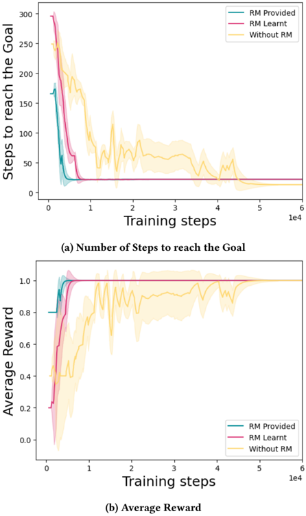## 4.1 ThreeButtons Task We evaluate our approach in the ThreeButtons task described in Example 2.1. The number of steps required to complete the task and the collective reward obtained by the team of agents throughout training are shown in Figure 3. The green curve shows the performance of the team of agents when the local RMs are manually engineered and provided. In pink , we show the performance of the team when the RMs are learnt. Finally in yellow , we show the performance of the team when each agent learn independently to perform their task without using the RM framework 1 . We observe that regardless of whether the local RMs are handcrafted or learned, the agents learn policies that, when combined, lead to the completion of the global task. Indeed, the collective reward obtained converges to the maximum reward indicating that all the agents have learnt to execute their sub-tasks and coordinate in order to achieve the common goal. Learning the RMs also helps speed up the learning for each of the agent, significantly reducing the number of training iterations required to learn to achieve the global task. We note however that the policy learnt without the RM framework requires less steps than when the RMs are used. 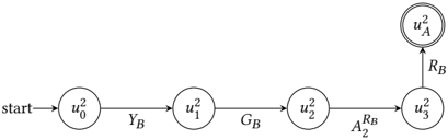We present in Figure 4 the RM learnt by 𝐴 2 using our interleaved learning approach. We compare it to the 'true' RM shown in Figure 2b. The back transition from 𝑢 2 3 to 𝑢 2 2 associated with the label 𝐴 ¬ 𝑅 𝐵 2 is missing from the learnt RM. This can be explained by the fact that this transition does not contribute towards the goal. When deriving the minimal RM from the set of labels, this one in particular is not deemed important and is thus ignored by the RM learner. 1 This is equivalent of using a 2-State RM, reaching the final state only when the task is completed. Figure 3: Comparison between handcrafted RMs (RM Provided) and our approach learning the RMs from traces (RM Learnt) in the ThreeButtons environment. <details> <summary>Image 3 Details</summary>  ### Visual Description ## Line Graphs: Performance Comparison with and without Reward Model (RM) ### Overview The image contains two line graphs comparing the performance of three training approaches: "RM Provided," "RM Learnt," and "Without RM." The graphs track metrics over training steps (x-axis: 0 to 10,000) and show how each method evolves in terms of efficiency (steps to goal) and effectiveness (average reward). --- ### Components/Axes #### Graph (a): Number of Steps to Reach the Goal - **X-axis**: Training steps (log scale, 0 to 10,000). - **Y-axis**: Steps to reach the goal (linear scale, 0 to 300). - **Legend**: - Teal: "RM Provided" - Pink: "RM Learnt" - Yellow: "Without RM" - **Shading**: Represents variability (confidence intervals or error margins). #### Graph (b): Average Reward - **X-axis**: Training steps (log scale, 0 to 10,000). - **Y-axis**: Average reward (linear scale, 0.0 to 1.0). - **Legend**: Same color coding as Graph (a). --- ### Detailed Analysis #### Graph (a): Steps to Reach the Goal 1. **RM Provided (Teal)**: - Starts at ~250 steps, drops sharply to ~50 steps by 1,000 training steps. - Stabilizes near 0 steps by 10,000 steps. - Shading indicates minimal variability after initial drop. 2. **RM Learnt (Pink)**: - Begins at ~200 steps, declines to ~50 steps by 1,000 steps. - Stabilizes near 0 steps by 10,000 steps. - Slightly higher variability than "RM Provided" during early training. 3. **Without RM (Yellow)**: - Starts at ~150 steps, fluctuates widely (peaks ~200 steps, troughs ~100 steps). - Gradually declines to ~50 steps by 10,000 steps. - Shading shows significant variability throughout training. #### Graph (b): Average Reward 1. **RM Provided (Teal)**: - Begins at ~0.2, rises sharply to ~0.9 by 1,000 steps. - Stabilizes near 1.0 by 10,000 steps. - Shading indicates tight confidence intervals after initial rise. 2. **RM Learnt (Pink)**: - Starts at ~0.1, increases to ~0.8 by 1,000 steps. - Reaches ~0.95 by 10,000 steps. - Slightly more variability than "RM Provided" during early training. 3. **Without RM (Yellow)**: - Begins at ~0.3, fluctuates between ~0.4 and ~0.7. - Peaks at ~0.7 by 10,000 steps. - Shading shows persistent variability, with no clear convergence. --- ### Key Observations 1. **Efficiency (Steps to Goal)**: - Both RM methods ("Provided" and "Learnt") outperform "Without RM" significantly, achieving near-zero steps to goal by 10,000 steps. - "Without RM" requires ~2–3× more steps to reach the goal compared to RM methods. 2. **Effectiveness (Average Reward)**: - RM methods achieve ~90–100% reward by 10,000 steps, while "Without RM" plateaus at ~70%. - "RM Provided" converges faster and more reliably than "RM Learnt." 3. **Variability**: - "Without RM" exhibits the highest variability in both metrics, suggesting unstable learning. - RM methods show tighter confidence intervals, indicating more consistent performance. --- ### Interpretation The data demonstrates that integrating a Reward Model (RM), whether provided or learnt, drastically improves both efficiency and effectiveness in training. - **RM Provided** acts as a strong baseline, enabling rapid convergence to optimal performance (near-zero steps and ~1.0 reward). - **RM Learnt** performs comparably but requires slightly more training steps to stabilize, likely due to the additional complexity of learning the RM itself. - **Without RM** struggles with both metrics, highlighting the critical role of RM in guiding exploration and reward optimization. The persistent variability in "Without RM" suggests that the agent lacks a structured reward signal, leading to suboptimal and inconsistent learning. This analysis aligns with reinforcement learning principles, where reward shaping (via RM) accelerates convergence and stabilizes training dynamics. </details> Figure 4: Learnt RM for 𝐴 2 . <details> <summary>Image 4 Details</summary>  ### Visual Description ## Diagram: Process Flow with Feedback Loop ### Overview The image depicts a sequential process flow with a feedback mechanism. It begins at a "start" node and progresses through four stages labeled \( u^2_0 \), \( u^2_1 \), \( u^2_2 \), and \( u^2_3 \). A feedback loop connects \( u^2_3 \) back to an earlier stage \( u^2_A \), creating a cyclical component. ### Components/Axes - **Nodes**: - `start`: Initial node. - \( u^2_0 \): First stage. - \( u^2_1 \): Second stage. - \( u^2_2 \): Third stage. - \( u^2_3 \): Fourth stage. - \( u^2_A \): Feedback target node. - **Arrows/Transitions**: - `Y_B`: Transition from \( u^2_0 \) to \( u^2_1 \). - `G_B`: Transition from \( u^2_1 \) to \( u^2_2 \). - `A_RB`: Transition from \( u^2_2 \) to \( u^2_3 \). - `R_B`: Feedback arrow from \( u^2_3 \) to \( u^2_A \). ### Detailed Analysis - **Flow Direction**: - The process starts at `start` and moves linearly through \( u^2_0 \rightarrow u^2_1 \rightarrow u^2_2 \rightarrow u^2_3 \). - A feedback loop (`R_B`) connects \( u^2_3 \) back to \( u^2_A \), suggesting iterative refinement or correction. - **Labels**: - All nodes use superscript notation (e.g., \( u^2_0 \)), possibly indicating squared values or a specific mathematical property. - Arrow labels (`Y_B`, `G_B`, `A_RB`, `R_B`) likely represent variables, functions, or operations governing transitions. ### Key Observations - The feedback loop (`R_B`) introduces cyclicality, implying the process may repeat or adjust based on \( u^2_3 \)'s output. - No numerical values or quantitative data are present; the diagram focuses on structural relationships. ### Interpretation This diagram likely represents a system with sequential stages and iterative feedback. The use of \( u^2 \) notation suggests mathematical or computational relevance, such as squared error terms, energy states, or algorithmic steps. The feedback loop (`R_B`) indicates that the final output (\( u^2_3 \)) influences an earlier stage (\( u^2_A \)), enabling corrections or optimizations. The labels (`Y_B`, `G_B`, `A_RB`) may correspond to system parameters, constraints, or transformation rules governing transitions between stages. No numerical trends or outliers are observable due to the absence of quantitative data. The diagram emphasizes process structure over measurable outcomes. </details> Learning the global RM was also attempted in this environment. Unfortunately, learning the minimal RM for the size of this problem is hard and the RM learner timed out after the 1 ℎ limit. 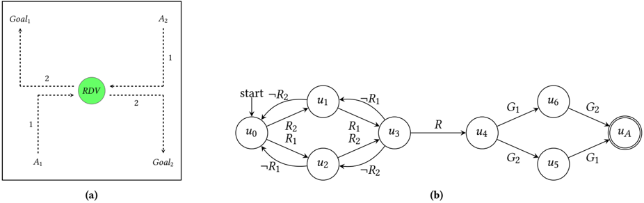## 4.2 Rendezvous Task The second environment in which we evaluate our approach is the 2-agent Rendezvous task [16] presented in Figure 5a. This task is composed of 2 agents acting in a grid with the ability to go up, down, left, right or do nothing. The task requires the agents to move in the environment to first meet in an 𝑅𝐷𝑉 location, i.e, all agents need to simultaneously be in that location for at least one timestep. Then each of the agents must reach their individual goal location for the global task to be completed. 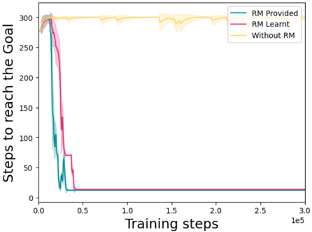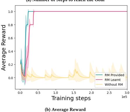We present in Figure 6 the number of steps (6a) to complete the task and the collective reward received by the team of agents (6b) throughout training. In green we show the performance when the RMs are known a priori and provided to the agents. This scenario, where we have perfect knowledge about the structure of each subtasks, is used as an upper bound for the results of our approach. In pink , we show the performances of our approach where the local RMs are learnt. The yellow curve shows the performance of the team when each agent learns to perform their individual task without the RM construct. The collective reward obtained while interleaving the learning of the policies and the learning of the local RMs converges to the maximum reward after a few iterations. In this task, the RM framework is shown to be crucial to help the team solve the task in a timely manner. Indeed, without the RMs (either known a priori or learnt), the team of agents do not succeed at solving the task. We also attempted to learn the global RM directly but the task could not be solved (i.e., a collective goal trace was not observed). The collective reward remained null throughout the training that we manually stopped after 1 𝑒 6 timesteps. ## 5 RELATED WORK Since the recent introduction of reward machines as a way to model non-Markovian rewards [19, 20], several lines of research have based their work on this concept (or similar finite-state machines). Most of the work has focused on how to derive them from logic specifications [1] or demonstrations [2], as well as learning them using different methods [3, 9-11, 13, 21, 22]. In this work, based on the multi-agent with RMs work by Neary et al. [16], the RMs of the different agents are executed in parallel. Recent works have considered other ways of composing RMs, such as merging the state and reward transition functions [6] or arranging them hierarchically by enabling RMs to call each other [10]. The latter is a natural way of extending this work since agents could share subroutines in the form of callable RMs. The policy learning algorithm for exploiting RMs we employ is an extension of the QRM algorithm (see Sections 2.2.2-2.2.3). However, algorithms based on making decisions at two hierarchical levels [9, 19] or more [10] have been proposed. In the simplest case (i.e., two levels), the agent first decides which transition to satisfy from a given RM state, and then decides which low-level actions to take to satisfy that transition. For example, if agent 𝐴 2 gets to state 𝑢 2 3 in Figure 2b, the decisions are: (1) whether to satisfy the transition labeled 𝐴 ¬ 𝑅 𝐵 2 or the one labeled 𝑅 𝐵 , and (2) given the chosen transition, act towards satisfying it. Unlike QRM, this method is not guaranteed to learn optimal policies; however, it enables lower-level sub-tasks to be reused while QRM does not. Note that the Q-functions learned by QRM depend on the structure of the whole RM and, hence, we learn them from scratch every time a new RM is induced. While other methods attempt to leverage the previously learned Q-functions [22], the hierarchical approach <details> <summary>Image 5 Details</summary>  ### Visual Description ## Diagram: Decision and Process Flow Schematics ### Overview The image contains two distinct diagrams: - **(a)** A decision tree with a central node labeled "RDV" connected to goals (Goal1, Goal2) and actions (A1, A2) via labeled arrows. - **(b)** A state transition diagram with nodes (u0–u6, uA) and transitions marked by labels like R1, R2, G1, G2, and R. ### Components/Axes #### Diagram (a): - **Central Node**: "RDV" (green circle, center of the square). - **Arrows**: - From RDV to **Goal1** (upward, labeled "1"). - From RDV to **Goal2** (downward, labeled "2"). - From RDV to **A1** (leftward, labeled "1"). - From RDV to **A2** (rightward, labeled "2"). - **Layout**: Dotted lines form a square around the central node. #### Diagram (b): - **Nodes**: - **Start**: u0 (labeled "start"). - **Intermediate**: u1, u2, u3, u4, u5, u6. - **Final**: uA (double-circle node). - **Transitions**: - **R1/R2**: Bidirectional arrows between u0, u1, u2, u3. - **R**: Unidirectional arrow from u3 to u4. - **G1/G2**: Arrows from u4 to u5/u6 and from u5/u6 to uA. - **Labels**: - "start" (arrow from u0). - "R", "G1", "G2" (transition labels). ### Detailed Analysis #### Diagram (a): - **Labels**: - Goals: Goal1, Goal2. - Actions: A1, A2. - Central node: RDV. - Arrow labels: "1" (Goal1, A1), "2" (Goal2, A2). - **Flow**: RDV is the decision point, with paths to goals and actions. The numbers on arrows may indicate priority, frequency, or step count. #### Diagram (b): - **Labels**: - Nodes: u0 (start), u1–u6, uA. - Transitions: R1, R2 (bidirectional), R (unidirectional), G1, G2 (unidirectional). - **Flow**: - Start at u0 → branches to u1 (R1) and u2 (R2). - u1 and u2 converge to u3 → u4 (R). - u4 branches to u5 (G2) and u6 (G1). - u5 and u6 converge to uA. - Direct path from u4 to uA via R. ### Key Observations - **Diagram (a)**: - Symmetrical layout with RDV as the focal point. - Arrows to goals and actions suggest a trade-off or decision between objectives and actions. - Numbers "1" and "2" may imply hierarchical or quantitative relationships (e.g., priority, cost, or steps). - **Diagram (b)**: - State transitions involve feedback loops (e.g., R1/R2 between u0, u1, u2). - G1/G2 transitions suggest group-specific pathways to the final state uA. - The direct R transition from u4 to uA implies a shortcut or alternative route. ### Interpretation - **Diagram (a)**: - RDV likely represents a decision variable or resource allocation point. - Goals (Goal1/Goal2) and actions (A1/A2) may reflect competing priorities or outcomes. - The numbers on arrows could indicate resource allocation (e.g., 1 unit to Goal1, 2 units to Goal2). - **Diagram (b)**: - The flowchart models a system with multiple states and transitions, possibly representing a process with feedback (e.g., R1/R2 loops) and group-specific outcomes (G1/G2). - The direct R transition from u4 to uA suggests a critical path or emergency route. - The use of "start" and "uA" implies a defined beginning and end state, typical of workflow or algorithmic processes. - **Cross-Diagram Relationships**: - Both diagrams use labeled nodes and transitions, suggesting they model decision-making or process flows. - RDV in (a) could correspond to a state in (b) (e.g., u4), with goals/actions mapping to transitions (e.g., G1/G2). ### Notes on Data and Structure - No numerical data beyond arrow labels (1, 2) or node labels (u0–u6, uA). - No explicit legend or color coding; diagrams rely on labels and spatial arrangement. - Spatial grounding: - Diagram (a): Central node (RDV) is at the center of the square. - Diagram (b): Nodes are arranged in a left-to-right, top-to-bottom sequence with branching. ### Conclusion The diagrams illustrate decision-making (a) and process flow (b) with explicit labels for nodes, transitions, and goals. While no numerical data is provided beyond labels, the structure suggests a focus on relationships, priorities, and state transitions. Further context (e.g., definitions of R1/R2, G1/G2) would clarify their meanings. </details> Figure 5: Example of the Rendezvous task where 2 agents must meet on the RDV point (green) before reaching their goal state 𝐺 1 and 𝐺 2 for agents 𝐴 1 and 𝐴 2 respectively. <details> <summary>Image 6 Details</summary>  ### Visual Description ## Line Chart: Steps to Reach the Goal ### Overview The chart compares the performance of three approaches in reaching a goal over training steps: "RM Provided," "RM Learnt," and "Without RM." The y-axis measures the number of steps required to reach the goal, while the x-axis represents training steps up to 300,000 (3.0e5). All three lines show a sharp decline in steps to reach the goal at the start of training, followed by stabilization. ### Components/Axes - **X-axis (Training steps)**: Logarithmic scale from 0.0 to 3.0e5 (300,000). - **Y-axis (Steps to reach the Goal)**: Linear scale from 0 to 300. - **Legend**: Located in the top-right corner, with three entries: - **RM Provided**: Teal line. - **RM Learnt**: Pink line. - **Without RM**: Yellow line. - **Shaded Regions**: Confidence intervals (error margins) around each line. ### Detailed Analysis 1. **RM Provided (Teal)**: - Starts at ~300 steps at 0.0 training steps. - Drops sharply to near 0 steps by ~0.5e5 training steps. - Remains flat at ~0 steps for the remainder of training. - Confidence interval is narrow after the initial drop, indicating consistent performance. 2. **RM Learnt (Pink)**: - Starts at ~300 steps at 0.0 training steps. - Drops sharply to near 0 steps by ~0.5e5 training steps, slightly delayed compared to "RM Provided." - Remains flat at ~0 steps for the remainder of training. - Confidence interval is slightly wider than "RM Provided" but stabilizes quickly. 3. **Without RM (Yellow)**: - Starts at ~300 steps at 0.0 training steps. - Remains flat at ~300 steps for the entire training period. - Confidence interval is wide, indicating high variability in performance. ### Key Observations - **Sharp Initial Drop**: Both "RM Provided" and "RM Learnt" achieve near-zero steps to reach the goal within ~0.5e5 training steps, suggesting rapid convergence. - **Baseline Underperformance**: "Without RM" fails to reduce steps to reach the goal, maintaining ~300 steps throughout training. - **Confidence Intervals**: "RM Provided" and "RM Learnt" show tight confidence intervals after the initial drop, while "Without RM" has wide intervals, reflecting instability. ### Interpretation The data demonstrates that reward models (RM) significantly accelerate goal achievement compared to training without them. "RM Provided" and "RM Learnt" both outperform the baseline by orders of magnitude, with "RM Provided" showing marginally faster convergence. The slight delay in "RM Learnt" may reflect the time required for the reward model to learn effective policies. The consistency of "RM Provided" suggests pre-trained reward models are more reliable than learned ones during early training phases. The absence of RM results in no improvement, highlighting its critical role in optimizing training efficiency. </details> (a) Number of Steps to reach the Goal Figure 6: Comparison between handcrafted RMs (RM Provided) and our approach learning the RMs from traces (RM Learnt) in the Rendezvous environment. <details> <summary>Image 7 Details</summary>  ### Visual Description ## Line Chart: Training Performance Comparison ### Overview The image contains two line charts comparing the performance of three training approaches: "RM Provided," "RM Learnt," and "Without RM." The charts track metrics across training steps (x-axis) and quantify efficiency ("Number of Steps to reach the Goal") and effectiveness ("Average Reward") (y-axis). ### Components/Axes - **Subplot (a): Number of Steps to reach the Goal** - **X-axis**: Training steps (0 to 3.0e5, logarithmic scale). - **Y-axis**: Average number of steps (0 to 1.0). - **Legend**: - Teal: "RM Provided" - Pink: "RM Learnt" - Yellow: "Without RM" - **Shaded Areas**: Confidence intervals (standard deviation) around each line. - **Subplot (b): Average Reward** - **X-axis**: Training steps (0 to 3.0e5, logarithmic scale). - **Y-axis**: Average reward (0 to 1.0). - **Legend**: Same color coding as subplot (a). ### Detailed Analysis #### Subplot (a): Number of Steps to Reach the Goal - **RM Provided (Teal)**: - Drops sharply from ~1.0 steps to near 0 by ~5e4 training steps. - Confidence interval narrows quickly, indicating stable performance. - **RM Learnt (Pink)**: - Similar steep decline to ~0 steps by ~5e4 steps. - Slightly higher variability than "RM Provided" (wider shaded area). - **Without RM (Yellow)**: - Remains flat at ~1.0 steps throughout training. - Confidence interval shows moderate variability (~0.1–0.2 steps). #### Subplot (b): Average Reward - **RM Provided (Teal)**: - Rises sharply from ~0.2 to ~0.8 reward by ~5e4 steps. - Plateaus near 0.8–0.9 reward. - **RM Learnt (Pink)**: - Similar trajectory to "RM Provided," peaking at ~0.8–0.9 reward. - Slightly lower peak (~0.7–0.8) compared to "RM Provided." - **Without RM (Yellow)**: - Fluctuates between ~0.0 and ~0.2 reward. - No clear upward trend; remains below 0.2 for most training steps. ### Key Observations 1. **RM Methods Outperform "Without RM"**: - Both "RM Provided" and "RM Learnt" achieve near-zero steps and high rewards (~0.8–0.9) within ~5e4 steps. - "Without RM" fails to improve, remaining at ~1.0 steps and <0.2 reward. 2. **Confidence Intervals**: - RM methods show tight confidence intervals, indicating consistent performance. - "Without RM" has wider variability but still inferior outcomes. 3. **Training Efficiency**: - RM methods converge rapidly, suggesting faster learning. ### Interpretation The data demonstrates that reinforcement models ("RM Provided" and "RM Learnt") significantly enhance training efficiency and effectiveness compared to training without reinforcement. The sharp decline in steps to reach the goal and rapid increase in average reward for RM methods highlight their critical role in optimizing performance. The minimal variability in RM methods’ confidence intervals further underscores their reliability. In contrast, the "Without RM" approach shows no improvement, emphasizing the necessity of reinforcement mechanisms for achieving high rewards and efficient learning. This aligns with reinforcement learning principles, where structured feedback (via RM) accelerates convergence to optimal solutions. </details> outlined here does not need to relearn all functions each time a new RM is induced. In the multi-agent community, the use of finite-state machines for task decomposition in collaborative settings has been studied in [4, 8] where a top-down approach is adopted to construct submachines from a global task. Unlike our work, these methods focus on the decomposition of the task but not on how to execute it. The algorithm presented in this paper interleaves both the decomposition and the learning of the policies associated with each state of the RM. The MARL community studying the collaborative setting has proposed different approaches to decompose the task among all the different agents. For example, QMIX [17] tackles the credit assignment problem in MARL assuming that the team's Q-function can be factorized, and performs a value-iteration method to centrally train policies that can be executed in a decentralised fashion. While this approach has shown impressive empirical results, its interpretation is more difficult than understanding the structure of the task using RM. The use of RMs in the MARL literature is starting to emerge. The work of Neary et al. [16] was the first to propose the use of RMs for task decomposition among multiple agents. As already mentioned in this paper, this work assumes that the structure of the task is known 'a priori', which is often untrue. With a different purpose, Dann et al. [5] propose to use RMs to help an agent predict the next actions the other agents in the system will perform. Instead of modeling the other agents' plan (or program), the authors argue that RMs provide a more permissive way to accommodate for variations in the behaviour of the other agent by providing a higher-level mechanism to specify the structure of the task. In this work as well, the RMs are pre-defined and provided to the agent. Finally, the work of Eappen and Jagannathan [7] uses a finitestate machine called 'task monitor', which is built from temporal logic specifications that encode the reward signal of the agents in the system. A task monitor is akin to an RM with some subtle differences like the use of registers for memory. ## 6 CONCLUSION AND FUTURE WORK Dividing a problem into smaller parts that are easier to solve is a natural approach performed instinctively by humans. It is also particularly suited for the multi-agent setting where all the available resources can be utilized to solve the problem or when a complementary set of skills is required. In this work, we extend the approach by Neary et al. [16], who leverage RMs for task decomposition in a multi-agent setting. We propose a novel approach where the RMs are learnt instead of manually engineered. The method presented in this paper interleaves the learning of the RM from the traces collected by the agent and the learning of the set of policies used to achieve the task's goal. Learning the RMs associated with each sub-task not only helps deal with non-Markovian rewards but also provides a more interpretable way to understand the structure of the task. We show experimentally in the ThreeButtons and the Rendezvous environments that our approach converges to the maximum reward a team of agents can obtain by collaborating to achieve a goal. Finally, we validated that the learnt RM corresponds indeed to the RM needed to achieve each sub-task. While our approach lifts the assumption about knowing the structure of the task 'a priori', a set of challenges remain and could be the object of further work: - (1) Alabeling function is assumed to exist for each of the agents and be known by them. In other words, each agent knows the labels relevant to its task and any labels used for synchronization with the other team members. - (2) If the labeling functions are noisy, agents may fail to synchronize and hence not be able to progress in their sub-tasks. In this scenario, the completion of the cooperative task is compromised. Defining or learning a communication protocol among the agents could be the object of future work. - (3) Our approach assumes that the global task has been automatically divided into several tasks, each to be completed by one of the agents. Dynamically creating these sub-tasks and assigning them to each of the agents is crucial to having more autonomous agents and would make an interesting topic for further research. - (4) We leverage task decomposition to learn simpler RMs that when run in parallel represent a more complex global RM. Task decomposition can be driven further through task hierarchies, which could be represented through hierarchies of RMs [10]. Intuitively, each RM in the hierarchy should be simpler to learn and enable reusability and further parallelization among the different agents. The use of RMs in the multi-agent context is still in its infancy and there are several exciting avenues for future work. We have demonstrated in this paper that it is possible to learn them under certain assumptions that could be relaxed in future work. ## ACKNOWLEDGMENTS Research was sponsored by the Army Research Laboratory and was accomplished under Cooperative Agreement Number W911NF-222-0243. The views and conclusions contained in this document are those of the authors and should not be interpreted as representing the official policies, either expressed or implied, of the Army Research Laboratory or the U.S. Government. The U.S. Government is authorised to reproduce and distribute reprints for Government purposes notwithstanding any copyright notation herein. ## REFERENCES - [1] Alberto Camacho, Rodrigo Toro Icarte, Toryn Q. Klassen, Richard Anthony Valenzano, and Sheila A. McIlraith. 2019. LTL and Beyond: Formal Languages for Reward Function Specification in Reinforcement Learning. In Proceedings of the International Joint Conference on Artificial Intelligence (IJCAI) . 6065-6073. - [2] Alberto Camacho, Jacob Varley, Andy Zeng, Deepali Jain, Atil Iscen, and Dmitry Kalashnikov. 2021. Reward Machines for Vision-Based Robotic Manipulation. In Proceedings of the IEEE International Conference on Robotics and Automation (ICRA) . 14284-14290. - [3] Phillip J. K. Christoffersen, Andrew C. Li, Rodrigo Toro Icarte, and Sheila A. McIlraith. 2020. Learning Symbolic Representations for Reinforcement Learning of Non-Markovian Behavior. In Proceedings of the Knowledge Representation and Reasoning Meets Machine Learning (KR2ML) Workshop at the Advances in Neural Information Processing Systems (NeurIPS) Conference . - [4] Jin Dai and Hai Lin. 2014. Automatic synthesis of cooperative multi-agent systems. In Proceedings of the IEEE Conference on Decision and Control (CDC) . 6173-6178. - [5] Michael Dann, Yuan Yao, Natasha Alechina, Brian Logan, and John Thangarajah. 2022. Multi-Agent Intention Progression with Reward Machines. In Proceedings of the International Joint Conference on Artificial Intelligence (IJCAI) . 215-222. - [6] Giuseppe De Giacomo, Marco Favorito, Luca Iocchi, Fabio Patrizi, and Alessandro Ronca. 2020. Temporal Logic Monitoring Rewards via Transducers. In Proceedings of the International Conference on Principles of Knowledge Representation and Reasoning (KR) . 860-870. - [7] Joe Eappen and Suresh Jagannathan. 2022. DistSPECTRL: Distributing Specifications in Multi-Agent Reinforcement Learning Systems. arXiv preprint arXiv:2206.13754 (2022). - [8] Ayman Elshenawy Elsefy. 2020. A task decomposition using (HDec-POSMDPs) approach for multi-robot exploration and fire searching. International Journal of Robotics and Mechatronics 7, 1 (2020), 22-30. - [9] Daniel Furelos-Blanco, Mark Law, Anders Jonsson, Krysia Broda, and Alessandra Russo. 2021. Induction and Exploitation of Subgoal Automata for Reinforcement Learning. J. Artif. Intell. Res. 70 (2021), 1031-1116. - [10] Daniel Furelos-Blanco, Mark Law, Anders Jonsson, Krysia Broda, and Alessandra Russo. 2022. Hierarchies of Reward Machines. arXiv preprint arXiv:2205.15752 (2022). - [11] Maor Gaon and Ronen I. Brafman. 2020. Reinforcement Learning with NonMarkovian Rewards. In Proceedings of the AAAI Conference on Artificial Intelligence (AAAI) . 3980-3987. - [12] E. Mark Gold. 1978. Complexity of Automaton Identification from Given Data. Inf. Control. 37, 3 (1978), 302-320. - [13] Mohammadhosein Hasanbeig, Natasha Yogananda Jeppu, Alessandro Abate, Tom Melham, and Daniel Kroening. 2021. DeepSynth: Automata Synthesis for Automatic Task Segmentation in Deep Reinforcement Learning. In Proceedings of the AAAI Conference on Artificial Intelligence (AAAI) . 7647-7656. - [14] Leslie Pack Kaelbling. 1993. Learning to Achieve Goals. In Proceedings of the International Joint Conference on Artificial Intelligence (IJCAI) . 1094-1099. - [15] Mark Law, Alessandra Russo, and Krysia Broda. 2015. The ILASP System for Learning Answer Set Programs. https://www.doc.ic.ac.uk/~ml1909/ILASP - [16] Cyrus Neary, Zhe Xu, Bo Wu, and Ufuk Topcu. 2021. Reward Machines for Cooperative Multi-Agent Reinforcement Learning. In Proceedings of the International Conference on Autonomous Agents and Multiagent Systems (AAMAS) . 934-942. - [17] Tabish Rashid, Mikayel Samvelyan, Christian Schroeder De Witt, Gregory Farquhar, Jakob Foerster, and Shimon Whiteson. 2020. Monotonic value function factorisation for deep multi-agent reinforcement learning. The Journal of Machine Learning Research 21, 1 (2020), 7234-7284. - [18] Richard S. Sutton and Andrew G. Barto. 2018. Reinforcement Learning: An Introduction . MIT Press. - [19] Rodrigo Toro Icarte, Toryn Klassen, Richard Valenzano, and Sheila McIlraith. 2018. Using Reward Machines for High-Level Task Specification and Decomposition in Reinforcement Learning. In Proceedings of the International Conference on Machine Learning (ICML) . 2107-2116. - [20] Rodrigo Toro Icarte, Toryn Q. Klassen, Richard Valenzano, and Sheila A. McIlraith. 2022. Reward Machines: Exploiting Reward Function Structure in Reinforcement Learning. J. Artif. Intell. Res. 73 (2022), 173-208. - [21] Rodrigo Toro Icarte, Ethan Waldie, Toryn Q. Klassen, Richard Anthony Valenzano, Margarita P. Castro, and Sheila A. McIlraith. 2019. Learning Reward Machines for Partially Observable Reinforcement Learning. In Proceedings of the Advances in Neural Information Processing Systems (NeurIPS) Conference . 15497-15508. - [22] Zhe Xu, Ivan Gavran, Yousef Ahmad, Rupak Majumdar, Daniel Neider, Ufuk Topcu, and Bo Wu. 2020. Joint Inference of Reward Machines and Policies for Reinforcement Learning. In Proceedings of the International Conference on Automated Planning and Scheduling (ICAPS) . 590-598.