## Parallel Neural Networks in Golang
Daniela Kalwarowskyj and Erich Schikuta
University of Vienna
Faculty of Computer Science, RG WST A-1090 Vienna, Währingerstr. 29, Austria dkalwarowskyj@yahoo.com erich.schikuta@univie.ac.at
Abstract. This paper describes the design and implementation of parallel neural networks (PNNs) with the novel programming language Golang. We follow in our approach the classical Single-Program Multiple-Data (SPMD) model where a PNN is composed of several sequential neural networks, which are trained with a proportional share of the training dataset. We used for this purpose the MNIST dataset, which contains binary images of handwritten digits. Our analysis focusses on different activation functions and optimizations in the form of stochastic gradients and initialization of weights and biases. We conduct a thorough performance analysis, where network configurations and different performance factors are analyzed and interpreted. Golang and its inherent parallelization support proved very well for parallel neural network simulation by considerable decreased processing times compared to sequential variants.
Keywords: Backpropagation Neuronal Network Simulation · Parallel and Sequential Implementation · MNIST · Golang Programming Language
## 1 Introduction
When reading a letter our trained brain rarely has a problem to understand its meaning. Inspired by the way our nervous system perceives visual input, the idea emerged to write a mechanism that could 'learn' and furthermore use this 'knowledge' on unknown data. Learning is accomplished by repeating exercises and comparing results with given solutions. The neural network studied in this paper uses the MNIST dataset to train and test its capabilities. The actual learning is achieved by using backpropagation. In the course of our research, we concentrate on a single sequential feed forward neural network (SNN) and upgrade it into building multiple, parallel learning SNNs. Those parallel networks are then fused to one parallel neural network (PNN). These two types of networks are compared on their accuracy, confidence, computational performance and learning speed, which it takes those networks to learn the given task.
The specific contribution of the paper is twofold: on the one hand, a thorough analysis of sequential and parallel implementations of feed forward neural
network respective time, accuracy and confidence, and on the other hand, a feasibility study of Golang [9] and its tools for parallel simulation.
The structure of the paper is as follows: In the next section, we give a short overview of related work. The parallelization approach is laid out in section 4 followed by the description of the Golang implementation. A comprehensive analysis of the sequential and parallel neural networks respective accuracy, confidence, computational performance and learning speed is presented in section 5. Finally, the paper closes with a summary of the findings.
## 2 Related Work and Baseline Research
Artificial neural networks and their parallel simulation gained high attention in the scientific community. Parallelization is a classic approach for speeding up execution times and exploiting the full potential of modern processors. Still, not every algorithm can profit from parallelization, as the concurrent execution might add a non-negligible overhead. This can also be the case for data parallel neural networks, where accuracy problems usually occur, as the results have to be merged.
In the literature a huge number of papers on parallelizing neural networks can be found. An excellent source of references is the survey by Tal Ben-Nun and Torsten Hoefler [1]. However, only few research was done on using Golang in this endeavour.
In the following only specific references are listed, which influenced the presented approach directly. The authors of [8] presented a parallel backpropagation algorithm dealing with the accuracy problem only by using a MapReduce and Cascading model. In the course of our work on parallel and distributed systems [16,2,14] we developed several approaches for the parallelization of neural networks. In [6], two novel parallel training approaches were presented for face recognizing backpropagation neural networks. The authors use the OpenMP environment for classic CPU multithreading and CUDA for parallelization on GPU architectures. Aside from that, they differentiated between topological data parallelism and structural data parallelism [15], where the latter is focus of the presented approach here. [10] gave a comparison of different parallelization approaches on a cluster computer. The results differed depending on the network size, data set sizes and number of processors. Besides parallelizing the backpropagation algorithm for training speed-up, alternative training algorithms like the Resilient Backpropagation described in [13] might lead to faster convergence. One major difference to standard backpropagation is that every weight and bias has a different and variable learning rate. A detailed comparison of both network training algorithms was given in [12] in the case of spam classification.
## 3 Fundamentals
In the following we present the mathematical fundamentals of neural networks to allow for easier understanding and better applicability of our implementation approach described afterwards.
Forwardpropagation To calculate an output in the last layer, the input values need to get propagated through each layer. This process is called forward propagation and is done by applying an activation function on each neuron's corresponding input sum. The input sum z for a neuron k in the layer l is the sum of each neuron's activation a from the last layer multiplied with the weight w :
$$z _ { k } ^ { l } = \sum _ { j } ( w _ { k j } ^ { l } a _ { j } ^ { l - 1 } + b _ { k } ^ { l } ) \quad ( 1 )$$
The additional term + b stands for the bias value, which allows the activation function to be shifted to the left or to the right. For better readability, the input sums for a whole layer can be stored in a vector z and defined by:
$$z ^ { l } = W ^ { l } x ^ { l - 1 } + b ^ { l } \quad ( 2 )$$
Here, W l is a weight matrix storing all weights to layer x l . To obtain the output of a layer, or, in case of the last layer x L , the output of a neural network, an activation function ϕ needs to be applied:
$$x ^ { l } = \varphi ( z ^ { l } ) = \varphi ( W ^ { l } x ^ { l - 1 } + b ^ { l } ) \quad ( 3 )$$
Activation functions do not have to be unique in a network and can be combined. The implementation presented in this paper uses the rectifier activation function
$$\varphi _ { r e c t i f i e r } ( z ) = \begin{cases} 0 & i f z < 0 \\ z & i f z \geq 0 \end{cases} ( 4 )$$
for hidden neurons and the softmax activation function
$$\varphi _ { s o f t \max } ( z _ { i } ) = \frac { e ^ { z _ { i } } } { \sum _ { j } e ^ { z _ { j } } } \quad ( 5 )$$
for output neurons. For classification, each class is represented by one neuron in the last layer. Due to the softmax function, the output values of those neurons sum up to 1 and can therefore be seen as the probabilities of being that class.
Backpropagation For proper classification the network has to be trained beforehand. In order to do that, a cost function tells us how well the network performs, like the cross entropy error with expected outputs e and actual outputs x ,
$$C = - \sum _ { i } e _ { i } \log ( x _ { i } ) & & ( 6 )$$
The aim is to minimize the cost function by finding the optimal weights and biases with the gradient descent optimization algorithm. Therefore, a training instance gets forward propagated through the network to get an output. Subsequently, it is necessary to compute the partial derivatives of the cost function with respect to each weight and bias in the network:
$$\frac { \partial C } { \partial w _ { k j } } = \frac { \partial C } { \partial z _ { k } } \frac { \partial z _ { k } } { \partial w _ { k j } }$$
$$\frac { \partial C } { \partial b _ { k } } = \frac { \partial C } { \partial z _ { k } } \frac { \partial z _ { k } } { \partial b _ { k j } }$$
As a first step, ∂C ∂z k needs to be calculated for every neuron k in the last layer L :
$$\delta _ { k } ^ { L } = \frac { \partial C } { \partial z _ { k } ^ { L } } = \frac { \partial C } { \partial x _ { k } ^ { L } } \varphi ^ { \prime } ( z _ { k } ^ { L } )$$
In case of the cross entropy error function, the error signal vector δ of the softmax output layer is simply the actual output vector minus the expected output vector:
$$\delta ^ { L } = \frac { \partial C } { \partial z ^ { L } } = x ^ { L } - e ^ { L } & & ( 1 0 )$$
To obtain the errors for the remaining layers of the network, the output layer's error signal vector δ L has to be propagated back through the network, hence the name of the algorithm:
$$\delta ^ { l } = ( W ^ { l + 1 } ) ^ { T } \delta ^ { l + 1 } \odot \varphi ^ { \prime } ( z ^ { l } ) \quad ( 1 1 )$$
( W l +1 ) T is the transposed weight matrix, denotes the Hadamard product or entry-wise product and ϕ ′ is the first derivative of the activation function.
Gradient Descent Knowing the error of each neuron, the changes to the weights and biases can be determined by
$$\Delta w _ { k j } ^ { l } = - \eta \frac { \partial C } { \partial w _ { k j } ^ { l } } = - \eta \delta _ { k } ^ { l } x _ { j } ^ { l - 1 } \quad ( 1 2 )$$
$$\Delta b _ { k } ^ { l } = - \eta \frac { \partial C } { \partial b _ { k } } = - \eta \delta _ { k } ^ { l }$$
The constant η is used to regulate the strength of the changes applied to the weights and biases and is also referred to as the learning rate, x l -1 j stands for the output of the j th neuron from layer l -1 . The changes are applied by adding them to the old weights and biases. Depending on the update frequency, a distinction is made between stochastic gradient descent, batch gradient descent and minibatch gradient descent. In the case of the first-mentioned, the weights and biases are updated after every training instance (by repeating all of the aforementioned steps instance-wise). In contrast, batch gradient descent stands for updating only once after accumulating the gradients of all training samples. Mini-batch gradient descent is a combination of both. The weights and biases are updated after a specified amount, the mini-batch size , of training instances. As with batch gradient descent, the gradients of all instances are averaged before the updates.
## 4 Parallel Neuronal Networks
This section describes the technology stack, the parallelization model and implementation details of the provided PNN.
## 4.1 Technology Stack
Go, often referred to as Golang, is a compiled, statically typed, open source programming language developed by a team at Google and released in November 2009. It is distributed under a BSD-style license, meaning that copying, modifying and redistributing is allowed under a few conditions.
As Andrew Gerrand, who works on the project, states in [9], Go grew from a dissatisfaction with the development environments and languages that they were using at Google. It is designed to be expressive, concise, clean and efficient. Hence, Go compiles quickly and is as easy to read as it is to write. This is partly because of gofmt, the go source code formatter, that gives Go programmes a single style and relieves the programmers from discussions like where to set the braces. As uniform presentation makes code easier to read and therefore to work on, gofmt also saves time and affects the scalability of programming teams [11]. The integrated garbage collector offers another great convenience and takes away the time consuming efforts on memory allocation and freeing known from C/C++. Despite the known overhead and criticism about Java's garbage collector, the author of [11] claims that Go is different, more efficient and that it is almost essential for a concurrent language like Go because of the trickiness that can result from managing ownership of a piece of memory as it is passed around among concurrent executions. That being said, built-in support for concurrency is one of the most interesting aspects of Go, offering a great advantage over older languages like C++ or Java. One major component of Go's concurrency model are goroutines, which can be thought of as lightweight threads with a negligible overhead, as the cost of managing them is cheap compared to threads. If a goroutine blocks, the runtime automatically moves any blocking code away from being executed and executes some code that can run, leading to highperformance concurrency [9]. Communication between goroutines takes place over channels, which are derived from "Communicating Sequential Processes" found in [5]. A Channel can be used to send and receive messages from the type associated with it. Since receiving can only be done when something is being sent, channels can be used for synchronization, preventing race conditions by design.
Another difference to common object oriented programming languages can be found in Go's object oriented design. Its approach misses classes and type-based inheritance like subclassing, meaning that there is no type hierarchy. Instead, Go features polymorphism with interfaces and struct embedding and therefore encourages the composition over inheritance principle. An Interface is a set of methods, which is implemented implicitly by all data types that satisfy the interface [11].
For the rest, files are organized in packages, with every source file starting with a package statement. Packages can be used by importing them via their unique path. If a package path in the form of an URL refers to a remote repository, the remote package can be fetched with the go get command and subsequently imported like a local package. Additionally, Go will not compile, if unused packages are being imported.
## 4.2 Parallelization Model
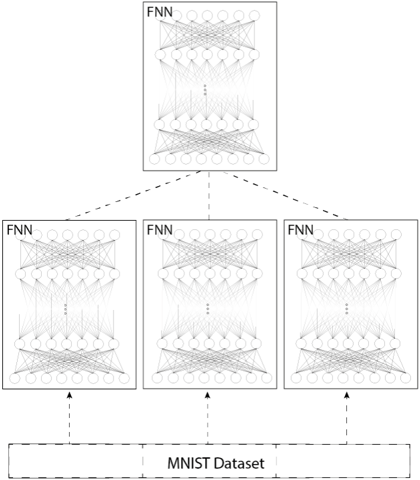
For the parallelization of neural network operations we apply the classical SingleProgram Multiple-Data (SPMD) approach well known from high-performance computing [3]. It is a programming technique, where several tasks execute the same program but with different input data and the calculated output data is merged to a common result. Thus, based on the fundamentals of single feed forward neural network we generate multiple of these networks and set them up to work together in parallel manner.
Fig. 1. Design of a Parallel Neural Network
<details>
<summary>Image 1 Details</summary>
### Visual Description
## Diagram: Ensemble of Feedforward Neural Networks (FNN)
### Overview
The image depicts a diagram of an ensemble of feedforward neural networks (FNNs) being trained on the MNIST dataset. The diagram shows three FNNs receiving input from the MNIST dataset, and their outputs are combined into a single FNN.
### Components/Axes
* **MNIST Dataset:** A rectangular box at the bottom of the diagram labeled "MNIST Dataset". This represents the input data source.
* **FNNs (Bottom Layer):** Three rectangular boxes, each labeled "FNN" in the top-left corner. Each box contains a simplified representation of a feedforward neural network, showing interconnected nodes arranged in layers.
* **FNN (Top Layer):** A single rectangular box at the top of the diagram, also labeled "FNN" in the top-left corner. This represents another feedforward neural network, presumably combining the outputs of the three FNNs in the bottom layer.
* **Connections:** Dashed arrows indicate the flow of data. Arrows point from the MNIST Dataset to each of the three FNNs in the bottom layer. Dashed lines also connect the three FNNs in the bottom layer to the single FNN in the top layer.
* **Nodes and Connections within FNNs:** Each FNN is represented by circles (nodes) arranged in layers, with lines connecting nodes in adjacent layers. The number of nodes per layer appears to vary. The connections between nodes are represented by thin gray lines.
### Detailed Analysis
* **MNIST Dataset:** The MNIST dataset serves as the input to the system.
* **Bottom Layer FNNs:** Each of the three FNNs in the bottom layer receives the MNIST dataset as input. The internal structure of each FNN consists of multiple layers of interconnected nodes. The number of nodes in each layer appears to decrease from input to output.
* **Top Layer FNN:** The outputs of the three FNNs in the bottom layer are fed into the single FNN in the top layer. This FNN likely combines the outputs of the three individual networks to produce a final prediction.
* **Network Structure:** The FNNs are represented as having multiple layers. The number of nodes in each layer varies, but generally decreases as the data flows through the network. The connections between nodes are dense, indicating that each node in one layer is connected to most or all nodes in the adjacent layer.
### Key Observations
* The diagram illustrates an ensemble learning approach, where multiple FNNs are trained on the same dataset and their outputs are combined.
* The use of three FNNs in the bottom layer suggests a potential for parallel processing or distributed training.
* The diagram is a high-level representation and does not provide specific details about the architecture of the FNNs (e.g., number of layers, number of nodes per layer, activation functions).
### Interpretation
The diagram represents a system for training a machine learning model using an ensemble of feedforward neural networks. The MNIST dataset is used as input, and the outputs of multiple FNNs are combined to improve the overall performance of the model. This approach can potentially improve accuracy and robustness compared to using a single FNN. The diagram highlights the flow of data and the relationships between the different components of the system. The ensemble method is used to improve the performance of the model by reducing variance and bias.
</details>
The parallel-design is visualized in figure 1. On the bottom it shows the dataset which is divided into as many slices as there are networks, referred to as child-networks (CN). Each child-network learns only a slice of the dataset. Ultimately the results of all parallel child-networks are merged to one final parallel
neural network (PNN). The combination of those CNs can be done in various ways. In the presented network the average of all weights, calculated by each parallel CN by a set number of epochs, is used for the PNNs weights. For the biases the same procedure is used, e.g. averaging all biases for the combined biases value.
In Golang it is important to take into consideration that a program, which is designed parallel does not necessarily work in a parallel manner, as a concurrent program can be parallel, but doesn't have to be. This programming language offers a goroutine, which 'is a function executing concurrently with other goroutines in the same address space' and processes with Go runtime. To start a goroutine a gofunc is called. It can an be equipped with a WaitGroup, that ensures that the process does not finish until all running processes are done. More about the implementation is explained in the next section.
## 4.3 Implementation Details
The main interface to which any trainable network binds is the TrainableNetwork interface. This interface is used throughout the whole learning and testing process. Parallel - as well as simple neural networks implement this interface. This allows for easy and interchangeable usage of both network types throughout the code. Due to the fact that a parallel neural network is built from multiple sequential neural networks (SNN) we start with the implementation of an SNN. The provided implementation of an SNN allows for a flexible network structure. For example, the number of layers and neurons, as well as the activationfunctions used on a layer, can be chosen freely. All information, required for creating a network is stored within a NeuroConfig struct on a network instance. These settings can easily be adjusted in a configuration file, the default name is config.yaml , located in the same directory as the executable.
A network is built out of layers. A minimal network is at least composed of an input layer and an output layer. Beyond this minimum, the hidden depth of a network can be freely adjusted by providing a desired number of hidden layers. Internally layers are represented by the NeuroLayer struct. A layer holds weights and biases which are represented by matrices. The Gonum package is used to simplify the implementation. It provides a matrix implementation as well as most necessary linear algebraic operations.
In the implementation, utility functions are provided for a convenient creation of new layers with initialized weights and biases. The library rand offers a function NormFloat 64 , where the variance is set 1 and the mean 0 as default. Weights are randomly generated using that normal distribution seeded by the current time in nanoseconds.
The provided network supports several activation functions. The activation function is defined on a per layer basis which enables the use of several activations within one network.
A PNN is a combination of at least two SNN. The ParallelNetwork struct represents the PNN in the implementation. As SNNs are trained individually before being combined with the output network of a PNN, it is necessary to
keep the references to the network managed in a slice. In the context of a PNN the SNNs are referred to as child networks (CN).
In a PNN the training process is executed on all CNs in parallel using goroutines. First, the dataset is split according to the amount of CNs. Afterwards, the slices of the training dataset and CNs are called with a goroutine. The goroutine executes minibatches of every CN in parallel. Within those minibatches, another mutexed concurrent goroutine is started for forwarding and backpropagating. Installing a mutex ensures safe access of the data over multiple goroutines.
The last step of training is to combine those CNs to one PNN. The provided network uses as combination function the "average" approach. After training the CNs for a set number of epochs, weights, and biases are added onto the PNN. Ultimately these weights and biases are scaled by the number of CNs. The result is the finished PNN.
## 5 Performance Evaluation
At first a test with one PNN, consisting of 10 CNs, and an SNN are tested using different activation functions on the hidden layer, while always using the softmax function on the output layer. After deciding on an activation function, network configurations are tested. While the number of neurons is only an observation, but not thoroughly tested, the number of networks is evaluated on different sized PNNs. Finally, the performance of both types of networks are compared upon time, accuracy, confidence and costs.
## 5.1 MNIST Dataset
For our analysis, we use the MNIST dataset which holds handwritten numbers and allows supervised learning. Using this dataset the network learns to read handwritten digits. Since learning is achieved by repeating a task, the MNIST dataset has a 'training-set of 60,000 examples, and a test-set of 10,000 examples' [7] . Each dataset is composed of an image-set and a label-set, which holds the information for the desired output and makes it possible to verify the networks output. All pictures are centered and uniform by 28x28 pixels. First, we start the training with the training-set. When the learning phase is over the network is supposed to be able to fulfill its task [8]. To evaluate it's efficiency it is tested by running the neural network with the test-set since the samples of this set are still unknown. It is important to use foreign data to test a network since it is more qualified to show the generalization of a network and therefore its true efficiency. We are aware that MNIST is a rather small data set. However, it was chosen on purpose, because it is used in many similar parallelization approaches and allows therefore for relatively easy comparison of results.
## 5.2 Activation Functions in Single- and Parallel Neuronal Networks
To elaborate which function performes best in terms of accuracy for the coded single- and parallel neural network a test using the same network design and
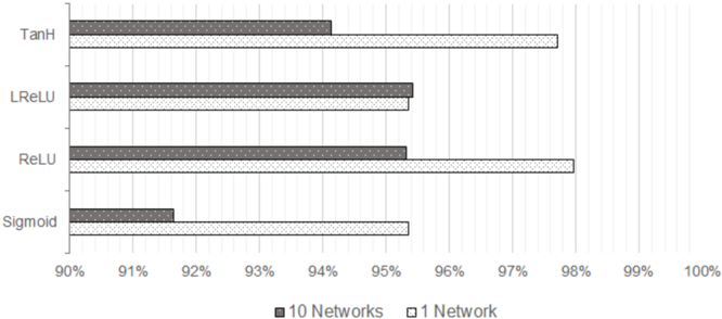
settings for each network is performed while changing only the function used on the hidden layer. Used settings were one hidden layer built out of 256 neurons, working with a batchsize of 50 and a learningrate η of 0.05 and an output layer calculated with softmax. This is used on a single FNN and a PNN each consisting of 10 child-networks. Figure 2 presents the performance results of the activation functions. Each networks setup is one hidden layer on which either the tangent hyperbolic-, leaky ReLU-, ReLU- or sigmoid-function was applied.
Fig. 2. Compare Accuracy of a parallel- vs simple-NN with different activation functions and a softmax function for the output layer. The networks have one hidden layer with 256 neurons and the training was performed with a learningrate of 0.05 and a batchsize of 50 over 20 epochs.
<details>
<summary>Image 2 Details</summary>
### Visual Description
## Horizontal Bar Chart: Activation Function Performance
### Overview
The image is a horizontal bar chart comparing the performance of different activation functions (TanH, LReLU, ReLU, Sigmoid) in neural networks. Performance is measured as a percentage, likely accuracy or a similar metric. The chart compares the performance of each activation function when used in a single network versus an ensemble of 10 networks.
### Components/Axes
* **Y-axis (Vertical):** Categorical axis listing the activation functions: TanH, LReLU, ReLU, Sigmoid.
* **X-axis (Horizontal):** Numerical axis representing performance percentage, ranging from 90% to 100% with tick marks at each percentage point.
* **Legend:** Located at the bottom of the chart.
* Dark Gray: "10 Networks"
* White with gray dots: "1 Network"
### Detailed Analysis
The chart displays the performance of each activation function for both a single network and an ensemble of 10 networks.
* **TanH:**
* 10 Networks (Dark Gray): Approximately 94%.
* 1 Network (White with gray dots): Approximately 97.8%.
* **LReLU:**
* 10 Networks (Dark Gray): Approximately 95.8%.
* 1 Network (White with gray dots): Approximately 95.2%.
* **ReLU:**
* 10 Networks (Dark Gray): Approximately 95.2%.
* 1 Network (White with gray dots): Approximately 97.6%.
* **Sigmoid:**
* 10 Networks (Dark Gray): Approximately 91.6%.
* 1 Network (White with gray dots): Approximately 93.0%.
### Key Observations
* For all activation functions, the performance is above 90%.
* Sigmoid has the lowest performance compared to the other activation functions.
* For TanH and ReLU, the performance of a single network is significantly higher than that of 10 networks.
* For LReLU, the performance of 10 networks is slightly higher than that of a single network.
* The performance difference between 1 network and 10 networks is minimal for LReLU.
### Interpretation
The chart suggests that the choice of activation function can significantly impact the performance of a neural network. The performance of TanH and ReLU is better in a single network, while LReLU performs slightly better in an ensemble of 10 networks. Sigmoid consistently shows the lowest performance, indicating it may not be the optimal choice for this particular task or network architecture. The fact that ensembling (10 networks) doesn't always improve performance suggests that the single network configurations for TanH and ReLU are already well-optimized, or that ensembling introduces other complexities that negate the benefits. The data implies that the optimal activation function and network configuration are highly dependent on the specific problem and architecture.
</details>
In this comparison the single neural network that learned using the ReLUfunction, closely followed by TanH-function, has reached the best result within 20 epochs. While testing different configurations it showed that most activation functions reached higher accuracy when using small learning rates. Sigmoid is one function that proved itself to be most efficient when the learningrate is not too small. By raising the learningrate to 0.6 the sigmoid-functions merit grows significantly on both network types. In the process of testing ReLU on hidden layers in combination with Softmax for the output layer has proven to reliably deliver good results. That is why in further sections ReLU has applied on all networks hidden layers and on the output layer Softmax.
## 5.3 Network Configurations
Number of Neurons. Choosing an efficient number of neurons is important, but it is hard to identify. There is no calculation which helps to define an effectively working number or range of neurons for a certain configuration of a
neural network. Varying the number of neurons between 20 to 600 delivered great accuracy. These are only observations and need to be studied with a more sophisticated approach.
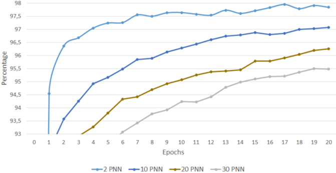
Number of Networks. To evaluate the performance of PNNs in terms of accuracy, PNNs with different amounts of CNs are composed and trained. The training runs over 20 epochs with a learning rate of 0.1 and a batchsize of 50. All CNs are built with one hidden layer consisting of 256 neurons. On the hidden layer the ReLU-function and on the output layer the Softmax-function is used. After every epoch, the networks are tested with the test-dataset. The results are visualized in figure 3.
Fig. 3. Accuracy of PNNs, built with different amount of CNs, over 20 epochs
<details>
<summary>Image 3 Details</summary>
### Visual Description
## Line Chart: PNN Performance vs. Epochs
### Overview
The image is a line chart comparing the performance of different Probabilistic Neural Networks (PNNs) based on the number of epochs. The chart displays the percentage (performance metric) on the y-axis against the number of epochs on the x-axis. Four different PNN configurations (2 PNN, 10 PNN, 20 PNN, and 30 PNN) are plotted, each represented by a distinct colored line.
### Components/Axes
* **X-axis:** Epochs, ranging from 0 to 20 in increments of 1.
* **Y-axis:** Percentage, ranging from 93 to 98 in increments of 0.5.
* **Legend:** Located at the bottom of the chart, associating each line color with a PNN configuration:
* Blue: 2 PNN
* Dark Blue: 10 PNN
* Olive/Brown: 20 PNN
* Light Gray: 30 PNN
### Detailed Analysis
* **2 PNN (Blue):** This line shows a rapid increase in percentage from epoch 1 to epoch 2, reaching approximately 96.5%. After epoch 2, the line plateaus and fluctuates slightly between 97.5% and 98% until epoch 20.
* Epoch 0: ~93%
* Epoch 1: ~96%
* Epoch 2: ~97%
* Epoch 20: ~97.8%
* **10 PNN (Dark Blue):** The line starts at approximately 93% at epoch 2 and gradually increases to approximately 97% by epoch 20. The slope decreases as the number of epochs increases.
* Epoch 2: ~93%
* Epoch 5: ~95%
* Epoch 10: ~96%
* Epoch 20: ~97%
* **20 PNN (Olive/Brown):** This line starts at approximately 93% at epoch 3 and increases to approximately 96% by epoch 20. The rate of increase slows down as the number of epochs increases.
* Epoch 3: ~93%
* Epoch 10: ~94.8%
* Epoch 20: ~96.2%
* **30 PNN (Light Gray):** This line starts at approximately 93% at epoch 4 and increases to approximately 95% by epoch 20. The rate of increase slows down as the number of epochs increases.
* Epoch 4: ~93%
* Epoch 10: ~94.2%
* Epoch 20: ~95.2%
### Key Observations
* The 2 PNN configuration achieves the highest percentage and plateaus quickly.
* The 10 PNN, 20 PNN, and 30 PNN configurations show a gradual increase in percentage with increasing epochs, with the 10 PNN configuration performing better than the 20 PNN and 30 PNN configurations.
* All configurations show diminishing returns with increasing epochs, as the rate of increase in percentage decreases.
### Interpretation
The chart suggests that the 2 PNN configuration is the most efficient, achieving high performance with fewer epochs. The other configurations (10 PNN, 20 PNN, and 30 PNN) require more epochs to reach comparable performance levels. The diminishing returns observed across all configurations indicate that there is a point beyond which increasing the number of epochs does not significantly improve performance. The data implies that the complexity of the PNN (number of PNN) has an inverse relationship with the speed of learning, but a direct relationship with the final performance. The 2 PNN model learns very quickly, but the other models eventually catch up.
</details>
Figure 3 illustrates a clear loss in accuracy of PNNs with a growing number of CNs. The 94.5% accuracy, for example, is reached by a PNN with 2 CNs after only one epoch, while a PNN with 30 CNs achieves that after 12 epochs. In respect to the number of networks this graph shows that more is not always better. Considering, that this test was only performed over a small number of epochs, it is not possible to read the potential of a PNN with more CNs. To find out how good a PNN can perform, a test was run with three PNNs running 300 epochs:
Table 1 shows a static growth until 200 epochs. After that, there is only a small fluctuation of accuracy, showing that a local minimum has been reached. Over the runtime of 300 epochs the difference of the performance regarding the accuracy of PNNs has been reduced significantly. Still the observation of the ranking of the PNNs has not been changed. The PNNs built out of a smaller
Table 1. Accuracy behaviour for different epochs
| CNs of PNN | Accuracy after... | Accuracy after... | Accuracy after... | Accuracy after... | Accuracy after... | Accuracy after... |
|--------------|------------------------------------------------------------------|------------------------------------------------------------------|------------------------------------------------------------------|------------------------------------------------------------------|------------------------------------------------------------------|------------------------------------------------------------------|
| | 20 Epochs 100 Epochs 150 Epochs 200 Epochs 250 Epochs 300 Epochs | 20 Epochs 100 Epochs 150 Epochs 200 Epochs 250 Epochs 300 Epochs | 20 Epochs 100 Epochs 150 Epochs 200 Epochs 250 Epochs 300 Epochs | 20 Epochs 100 Epochs 150 Epochs 200 Epochs 250 Epochs 300 Epochs | 20 Epochs 100 Epochs 150 Epochs 200 Epochs 250 Epochs 300 Epochs | 20 Epochs 100 Epochs 150 Epochs 200 Epochs 250 Epochs 300 Epochs |
| 2 | 97.76 | 98.08 | 98.13 | 98.16 | 98.14 | 98.17 |
| 10 | 96.58 | 97.43 | 97.96 | 98.03 | 98.09 | 98.05 |
| 20 | 95.69 | 97.50 | 97.71 | 97.92 | 97.90 | 97.97 |
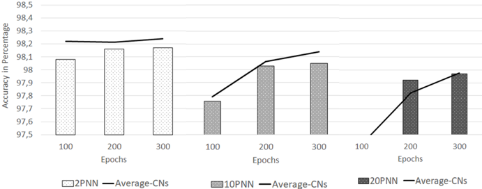
number of CNs perform slightly better. Since the provided PNNs are built by using averaging of weights and biases it also seemed interesting to compare the average accuracy of the CNs with the resulting PNN, to grade the used combination function. The results are illustrated in figure 4.
Fig. 4. Compare the average accuracy of all CNs, out of which the final PNN is formed, with that PNNs accuracy
<details>
<summary>Image 4 Details</summary>
### Visual Description
## Bar and Line Chart: Accuracy in Percentage vs Epochs for Different PNN Configurations
### Overview
The image is a bar and line chart comparing the accuracy (in percentage) of three different PNN (Probabilistic Neural Network) configurations (2PNN, 10PNN, and 20PNN) across varying numbers of epochs (100, 200, and 300). The chart displays the accuracy of each PNN configuration as bars, and the average accuracy of CNs (Convolutional Networks) as lines.
### Components/Axes
* **X-axis:** "Epochs" with markers at 100, 200, and 300. The x-axis is repeated for each PNN configuration.
* **Y-axis:** "Accuracy in Percentage" with markers from 97.5 to 98.5, incrementing by 0.1.
* **Legend (bottom):**
* Light gray bars: "2PNN"
* Black line: "Average-CNs"
* Medium gray bars: "10PNN"
* Dark gray bars: "20PNN"
### Detailed Analysis
**2PNN Configuration (Light Gray Bars):**
* At 100 Epochs: Accuracy is approximately 98.08%.
* At 200 Epochs: Accuracy is approximately 98.17%.
* At 300 Epochs: Accuracy is approximately 98.18%.
* Trend: The accuracy increases slightly from 100 to 200 epochs, then plateaus from 200 to 300 epochs.
**10PNN Configuration (Medium Gray Bars):**
* At 100 Epochs: Accuracy is approximately 97.76%.
* At 200 Epochs: Accuracy is approximately 98.00%.
* At 300 Epochs: Accuracy is approximately 98.05%.
* Trend: The accuracy increases from 100 to 200 epochs, then plateaus from 200 to 300 epochs.
**20PNN Configuration (Dark Gray Bars):**
* At 100 Epochs: Accuracy is approximately 97.50%.
* At 200 Epochs: Accuracy is approximately 97.92%.
* At 300 Epochs: Accuracy is approximately 97.97%.
* Trend: The accuracy increases from 100 to 200 epochs, then plateaus from 200 to 300 epochs.
**Average-CNs (Black Lines):**
* **For 2PNN:** The line starts at approximately 98.22% at 100 epochs, dips slightly to approximately 98.20% at 200 epochs, and then increases to approximately 98.24% at 300 epochs.
* **For 10PNN:** The line starts at approximately 97.85% at 100 epochs, increases to approximately 98.10% at 200 epochs, and then increases to approximately 98.14% at 300 epochs.
* **For 20PNN:** The line starts at approximately 97.50% at 100 epochs, increases to approximately 97.85% at 200 epochs, and then increases to approximately 97.95% at 300 epochs.
### Key Observations
* The 2PNN configuration consistently achieves the highest accuracy among the three PNN configurations.
* The accuracy of all PNN configurations generally increases as the number of epochs increases from 100 to 200, but the increase is less pronounced from 200 to 300 epochs.
* The Average-CNs accuracy generally increases with the number of epochs for all PNN configurations.
* The 2PNN configuration has the highest Average-CNs accuracy, while the 20PNN configuration has the lowest.
### Interpretation
The chart suggests that the 2PNN configuration is the most effective among the three PNN configurations tested, as it consistently achieves the highest accuracy. The increasing accuracy with more epochs (up to 200) indicates that the models are learning and improving their performance. The plateauing of accuracy from 200 to 300 epochs suggests that the models may be approaching their maximum potential performance, and further training may not yield significant improvements. The Average-CNs accuracy follows a similar trend, indicating that the convolutional networks are also benefiting from increased training. The differences in Average-CNs accuracy across the PNN configurations may be due to the specific characteristics of each configuration and how they interact with the convolutional networks.
</details>
It shows that the efficiency of an average function grows with the number of CNs. The first graph drawn with 2 CNs shows, that the resulting PNN is performing worse than the average of the CNs, it has been built from. By growing the number of CNs to 10, the average of CNs approximates towards the PNN. The last graph of this figure shows that a PNN composed of 20 CNs outperforms the average of its CNs after 200 epochs, and after 300 epochs levels with it. It has to be noted that the differences in accuracy are very small, as it is only a range of 0.1 to 0.2 percent. Overall it can be said that this combination function is working efficiently.
## 5.4 Comparing the Performances
Time. Time is the main reason to have a network working in parallel. To test the effect of parallelism on the time required to train a PNN, the provided neuronal
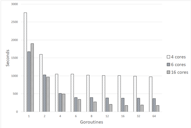
network is tested on three systems. The first system is equipped with 4 physical and 4 logical cores, an Intel i7-3635QM processor working with a basic clock rate of 2.4GHz, the second system holds 6 physical cores and 6 logical cores working with 2.9GHz and an Intel i9-8950HK processor and last the third system works with an AMD Ryzen Threadripper 1950X with 16 physical and 16 logical cores, which work with a clock rate of 3.4GHz. The first, second and third systems are referred to as 4 core, 6 core and 16 core in the following.
Fig. 5. Time in seconds, that was needed to train a PNN with a limited amount of one Goroutine per composed CN.
<details>
<summary>Image 5 Details</summary>
### Visual Description
## Bar Chart: Goroutines vs. Execution Time
### Overview
The image is a bar chart comparing the execution time (in seconds) of a program using different numbers of goroutines (1, 2, 4, 6, 8, 12, 16, 32, 64) on systems with 4, 6, and 16 cores. The chart shows how the execution time changes as the number of goroutines increases for each core configuration.
### Components/Axes
* **X-axis:** Goroutines (1, 2, 4, 6, 8, 12, 16, 32, 64)
* **Y-axis:** Seconds (0 to 3000, with increments of 500)
* **Legend (Top-Right):**
* White with dots: 4 cores
* Gray: 6 cores
* Dark Gray with dots: 16 cores
### Detailed Analysis
**4 Cores (White with dots):**
* Trend: Execution time decreases sharply from 1 to 2 goroutines, then decreases more gradually until 4 goroutines, and then remains relatively constant.
* 1 Goroutine: ~2750 seconds
* 2 Goroutines: ~1600 seconds
* 4 Goroutines: ~1050 seconds
* 6 Goroutines: ~1050 seconds
* 8 Goroutines: ~1050 seconds
* 12 Goroutines: ~1050 seconds
* 16 Goroutines: ~1050 seconds
* 32 Goroutines: ~1050 seconds
* 64 Goroutines: ~1000 seconds
**6 Cores (Gray):**
* Trend: Execution time decreases sharply from 1 to 2 goroutines, then decreases more gradually until 16 goroutines, and then remains relatively constant.
* 1 Goroutine: ~1700 seconds
* 2 Goroutines: ~1000 seconds
* 4 Goroutines: ~500 seconds
* 6 Goroutines: ~400 seconds
* 8 Goroutines: ~350 seconds
* 12 Goroutines: ~300 seconds
* 16 Goroutines: ~200 seconds
* 32 Goroutines: ~200 seconds
* 64 Goroutines: ~200 seconds
**16 Cores (Dark Gray with dots):**
* Trend: Execution time decreases sharply from 1 to 2 goroutines, then decreases more gradually until 16 goroutines, and then remains relatively constant.
* 1 Goroutine: ~1900 seconds
* 2 Goroutines: ~950 seconds
* 4 Goroutines: ~500 seconds
* 6 Goroutines: ~350 seconds
* 8 Goroutines: ~400 seconds
* 12 Goroutines: ~400 seconds
* 16 Goroutines: ~350 seconds
* 32 Goroutines: ~400 seconds
* 64 Goroutines: ~200 seconds
### Key Observations
* For all core configurations, increasing the number of goroutines initially results in a significant reduction in execution time.
* The execution time plateaus after a certain number of goroutines, suggesting diminishing returns.
* The 6-core configuration generally has the lowest execution time for higher numbers of goroutines.
* The 4-core configuration has the highest execution time across all numbers of goroutines.
### Interpretation
The data suggests that using goroutines can significantly improve the performance of a program, especially when the number of goroutines is optimized for the number of available cores. The initial decrease in execution time with increasing goroutines indicates that the program can effectively utilize concurrency. However, the plateauing effect suggests that there is an optimal number of goroutines beyond which adding more does not lead to further performance gains, and may even introduce overhead.
The 6-core configuration appears to be the most efficient in this scenario, achieving the lowest execution times for a wide range of goroutine counts. This could be due to a better match between the program's concurrency requirements and the available hardware resources on the 6-core system. The 4-core system consistently performs the worst, likely due to its limited ability to handle a large number of concurrent goroutines.
</details>
In figure 5 the benefit in terms of time using parallelism is clearly visible. The results illustrated show the average time in seconds needed by each system for training a PNN consisting of one CN per goroutine. For the block diagram in 5 the percental time requirements in comparison with the time needed using one goroutine are listed in table 2.
The time in figure 5 starts on a high level and decreases with an increasing amount of goroutines for all three systems. Especially in the range of 1 to 4 goroutines, a formidable decrease in training time is visible and only starts to level out when reaching a systems physical core limitation. This means that the 4 core starts to level out after 4 goroutines, the 6 core after 6 goroutines and the 16 core after 16 goroutines, even though all systems support hyper threading. After reaching a systems core number the average time necessary for training a neural network decreases further with more goroutines. This should be due to the ability to work in parallel and in concurrency as one slot finishes and a
Table 2. Average time required to train a PNN in comparison to one goroutine, which represents 100 percent
| | Time required compared to 1 goroutine | Time required compared to 1 goroutine | Time required compared to 1 goroutine | Time required compared to 1 goroutine | Time required compared to 1 goroutine | Time required compared to 1 goroutine | Time required compared to 1 goroutine | Time required compared to 1 goroutine | Time required compared to 1 goroutine |
|-------------------|-----------------------------------------|-----------------------------------------|-----------------------------------------|-----------------------------------------|-----------------------------------------|-----------------------------------------|-----------------------------------------|-----------------------------------------|-----------------------------------------|
| System/Goroutines | 1 | 2 | 4 | 6 | 8 | 12 | 16 | 32 | 64 |
| 4 | 100% | 58% | 38% | 38% | 37% | 37% | 37% | 36% | 35% |
| 6 | 100% | 61% | 31% | 24% | 24% | 23% | 23% | 23% | 22% |
| 16 | 100% | 51% | 26% | 18% | 14% | 11% | 9% | 10% | 9% |
waiting thread can start running immediately, without waiting for the rest of the running threads to be finished. All three systems show high time savings by parallelizing the neural networks. While time requirements decreased in every system, the actual time savings differ greatly as the 16 core system decreased 91 percent on average from 1 goroutine to 64 goroutines. In comparison, the 4 core system only took 65 percent less time. As the 16 core system is a lot more powerful than the 4 core system, it can perform an even greater parallel task and therefore displays a positive effect of parallelism upon time requirements. Based upon figure 5 and its table 2 parallelism within neural networks can be seen as a useful feature.
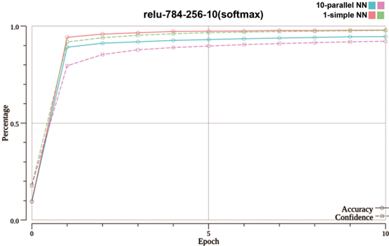
Fig. 6. Compare Accuracy and Confidence of a PNN composed of 10 CNs and an SNN with one Hidden Layer which holds 256 Neurons
<details>
<summary>Image 6 Details</summary>
### Visual Description
## Line Chart: ReLU-784-256-10 (softmax) Accuracy and Confidence
### Overview
The image is a line chart comparing the accuracy and confidence of two neural network architectures: a "10-parallel NN" and a "1-simple NN". The chart plots the percentage (accuracy/confidence) on the y-axis against the epoch number on the x-axis.
### Components/Axes
* **Title:** relu-784-256-10(softmax)
* **X-axis:**
* Label: Epoch
* Scale: 0 to 10, with tick marks at 0, 5, and 10.
* **Y-axis:**
* Label: Percentage
* Scale: 0.0 to 1.0, with tick marks at 0.0, 0.5, and 1.0.
* **Legend (Top-Right):**
* 10-parallel NN (Teal)
* 1-simple NN (Salmon)
* Accuracy (Teal, circle marker)
* Confidence (Salmon, square marker)
### Detailed Analysis
* **10-parallel NN (Teal Line):** The accuracy of the 10-parallel NN increases sharply from epoch 0 to approximately epoch 2, reaching a percentage of approximately 0.95. After epoch 2, the accuracy continues to increase, but at a much slower rate, reaching approximately 0.97 by epoch 10.
* Epoch 0: ~0.1
* Epoch 2: ~0.95
* Epoch 10: ~0.97
* **1-simple NN (Salmon Line):** The accuracy of the 1-simple NN also increases sharply from epoch 0 to approximately epoch 2, reaching a percentage of approximately 0.95. After epoch 2, the accuracy continues to increase, but at a much slower rate, reaching approximately 0.98 by epoch 10.
* Epoch 0: ~0.1
* Epoch 2: ~0.95
* Epoch 10: ~0.98
* **Confidence of 10-parallel NN (Dashed Pink Line with Square Markers):** The confidence of the 10-parallel NN increases sharply from epoch 0 to approximately epoch 2, reaching a percentage of approximately 0.85. After epoch 2, the confidence continues to increase, but at a much slower rate, reaching approximately 0.92 by epoch 10.
* Epoch 0: ~0.1
* Epoch 2: ~0.85
* Epoch 10: ~0.92
* **Confidence of 1-simple NN (Dashed Gray Line with Square Markers):** The confidence of the 1-simple NN increases sharply from epoch 0 to approximately epoch 2, reaching a percentage of approximately 0.85. After epoch 2, the confidence continues to increase, but at a much slower rate, reaching approximately 0.92 by epoch 10.
* Epoch 0: ~0.1
* Epoch 2: ~0.85
* Epoch 10: ~0.92
### Key Observations
* Both neural network architectures show a rapid increase in accuracy and confidence during the first few epochs.
* The accuracy of the 1-simple NN is slightly higher than the accuracy of the 10-parallel NN after epoch 2.
* The confidence of both networks is lower than their accuracy.
* The confidence of both networks appears to converge to the same value.
### Interpretation
The chart suggests that both the 10-parallel NN and the 1-simple NN architectures are effective in this task, with the 1-simple NN performing slightly better in terms of accuracy after the initial epochs. The lower confidence scores compared to accuracy scores may indicate that the models are sometimes making correct predictions without being entirely certain. The convergence of confidence scores suggests that both models may be reaching a similar level of certainty as they continue to train. The rapid increase in accuracy and confidence in the initial epochs highlights the importance of early training stages.
</details>
Accuracy and Confidence of Networks. In this section the performance in terms of accuracy and confidence is compared between a PNNs and an SNN.
For the test, illustrated by figure 6, both types of networks have been provided with the same random network to start their training. They have the exact same built, except that one is trained as SNN and the other is cloned 10 times to build a PNN with 10 CNs.
In figure 6 the SNN performs better than the PNN in both accuracy and confidence. While the SNNs accuracy and confidence overlap after 8 epochs, the PNN has a gap between both lines at all times. This concludes that the SNN is "sure" about its outputs, while the PNN is more volatile. The SNNs curve of confidence is a lot steeper than the PNNs and quickly approximates towards the curve of accuracy. Both curves of accuracy start off almost symmetric upwards the y-axis, but the PNN levels horizontally after about 90 percent while the SNN still rises until about 94 percent. After those points both accuracy curves run almost horizontally and in parallel towards the x-axis. The gap stays constantly until the end of the test. Even small changes within the range of 90 to 100 percent are to be interpreted as significant. This makes the SNN perform considerable more efficient in terms of accuracy and costs than the PNN.
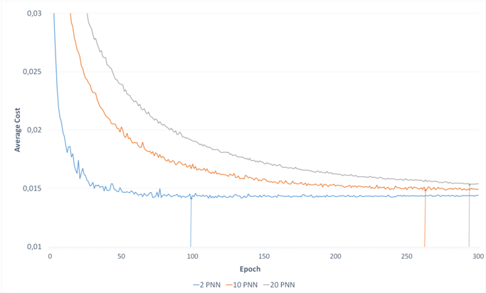
Cost of Networks. To see how successful the training of different PNNs are, the costs of 3 parallel networks with a varying number of CNs have been recorded for 300 epochs. The results are illustrated in figure 7.
Fig. 7. Average Costs of PNNs over 300 epochs. The vertical lines show the lowest cost for each PNN.
<details>
<summary>Image 7 Details</summary>
### Visual Description
## Line Chart: Average Cost vs. Epoch for Different PNN Configurations
### Overview
The image is a line chart comparing the average cost (error) of three different Probabilistic Neural Network (PNN) configurations (2 PNN, 10 PNN, and 20 PNN) over 300 epochs. The chart illustrates how the average cost decreases with increasing epochs for each configuration, eventually plateauing.
### Components/Axes
* **X-axis:** Epoch, ranging from 0 to 300 in increments of 50.
* **Y-axis:** Average Cost, ranging from 0.01 to 0.03 in increments of 0.005.
* **Legend:** Located at the bottom of the chart.
* Blue line: 2 PNN
* Orange line: 10 PNN
* Gray line: 20 PNN
### Detailed Analysis
* **2 PNN (Blue Line):**
* Trend: The average cost decreases rapidly in the initial epochs and then plateaus.
* Approximate Values: Starts around 0.03, drops to approximately 0.015 by epoch 50, and stabilizes around 0.014-0.015 after epoch 100.
* **10 PNN (Orange Line):**
* Trend: The average cost decreases steadily and then plateaus.
* Approximate Values: Starts around 0.03, drops to approximately 0.017 by epoch 100, and stabilizes around 0.015 after epoch 200.
* **20 PNN (Gray Line):**
* Trend: The average cost decreases gradually and then plateaus.
* Approximate Values: Starts around 0.03, drops to approximately 0.02 by epoch 100, and stabilizes around 0.016-0.017 after epoch 250.
### Key Observations
* All three PNN configurations show a decreasing trend in average cost as the number of epochs increases.
* The 2 PNN configuration shows the most rapid initial decrease in average cost but also exhibits more fluctuation.
* The 20 PNN configuration shows the slowest initial decrease in average cost but appears to stabilize more smoothly.
* After approximately 200 epochs, the average cost for all three configurations converges to a similar range (0.014-0.017).
### Interpretation
The chart demonstrates the learning process of the PNN models. As the models are trained over more epochs, their average cost (error) decreases, indicating improved performance. The different PNN configurations exhibit varying learning rates and stability. The 2 PNN configuration learns quickly but is less stable, while the 20 PNN configuration learns more slowly but is more stable. The convergence of the average cost for all configurations after a sufficient number of epochs suggests that there is a limit to the improvement achievable with further training. The choice of PNN configuration may depend on the specific application and the trade-off between learning speed and stability.
</details>
It shows that the costs of all three PNNs sink rapidly within the first 50 epochs. Afterwards, the error decreases slower, drawing a soft curve that flats out towards a line, almost stagnating. Apparently, all PNNs training moves fast towards a minimum at the beginning, then slows down and finally gets stuck, while only moving slightly up and down the minimums borders. Similar to earlier tests, a PNN built with less CNs performs better. More CNs leave the graph further up the y-axis, as the 2-PNN outperforms both the 10- and 20PNN. It also reaches its best configuration, e.g. the point where costs are lowest, significantly earlier than the other tested PNNs. Whereas the 10- and 20-PNNs work out their best performance regarding the costs at a relatively close range of epochs, they reach it late compared to the 2-PNN. Figure 7 clearly shows a decrease in quality with PNNs, formed with more CNs. This indicates that the combination function needs optimization to achieve a better graph. In the long term,F costs behave the same as accuracy. After 300 epochs the difference has almost leveled.
## 6 Findings and Conclusion
This paper presents and analyses PNNs composed of several sequential neural networks. The PNNs are tested upon time, accuracy and costs and compared to an SNN.
The parallelization approach on three different multicore systems show excellent speedup (the time necessary for training a PNN reduces constantly by increasing the number of CNs e.g. number of goroutines).
With all three tested systems the time necessary for training a PNN decreased constantly by increasing the number of CNs e.g. number of goroutines. While the difference in time was significant within the first few added goroutines it leveled out after reaching the systems number of cores. A PNN with 2 CNs takes 40% to 50% less time than a SNN and a PNN with 4 CNs takes 60% to 70% less time.
While time is a strong point of the PNN, accuracy is also dependent on the number of CNs a PNN is formed from. While a few CNs resulted in longer training times it generated better accuracy in fewer epochs. More CNs made the training time faster but the learning process slower. After 20 epochs a PNN composed of 2 CNs reached an accuracy of almost 98%, while a PNN composed of 20 CNs only slightly overcame the 96% line. When both PNNs were trained for a longer period this difference shrank dramatically. Trained for 300 epochs the accuracy only differed by 0.2% in favor of the PNN made out of 2 CNs. While this proved the ability to learn with a small data set it also demonstrated that bigger data sets deliver a better result faster. the PNNs can improve by 0.41% and 2.28% when training for a longer period. These results were achieved by using averaging as combination function. The chances of achieving an even better accuracy by improving the combination function are high. The costs of a PNN also depends on the number of CNs. It has the same behavior as accuracy and can also be improved by an optimized combination function. However, a
thorough analysis on the effects of improved combination functions is planned for future work and is beyond the scope of this paper.
Summing up, PNNs proved to be very time efficient but are still lacking in terms of accuracy. As there are plenty of other optimizations, e.g. adjusting learning rates [4], a PNN proved to be more time efficient than an SNN. However, until the issue of accuracy has been taken care of, the SNN surpasses the PNN in practice.
We close the paper with a final word on the feasibility of Golang for parallel neural network simulation: Data parallelism proved to be an efficient parallelization strategy. In combination with the programming language Go, a parallel neural network implementation is coded as fast as a sequential one, as no special efforts are necessary for concurrent programming thanks to Go's concurrency primitives, which offer a simple solution for multithreading.
## References
1. Ben-Nun, T., Hoefler, T.: Demystifying parallel and distributed deep learning: An in-depth concurrency analysis. ACM Computing Surveys (CSUR) 52 (4), 1-43 (2019)
2. Brezany, P., Mueck, T.A., Schikuta, E.: A software architecture for massively parallel input-output. In: Waśniewski, J., Dongarra, J., Madsen, K., Olesen, D. (eds.) Applied Parallel Computing Industrial Computation and Optimization. pp. 85-96. Springer Berlin Heidelberg, Berlin, Heidelberg (1996)
3. Darema, F.: The spmd model: Past, present and future. In: European Parallel Virtual Machine/Message Passing Interface Users' Group Meeting. pp. 1-1. Springer (2001)
4. Goyal, P., Dollár, P., Girshick, R., Noordhuis, P., Wesolowski, L., Kyrola, A., Tulloch, A., Jia, Y., He, K.: Accurate, large minibatch sgd: Training imagenet in 1 hour. arXiv preprint arXiv:1706.02677 (2017)
5. Hoare, C.A.R.: Communicating sequential processes. In: The origin of concurrent programming, pp. 413-443. Springer (1978)
6. Huqqani, A.A., Schikuta, E., Ye, S., Chen, P.: Multicore and gpu parallelization of neural networks for face recognition. Procedia Computer Science 18 (Supplement C), 349 - 358 (2013), 2013 International Conference on Computational Science
7. LeCun, Y., Bottou, L., Bengio, Y., Haffner, P.: Gradient-based learning applied to document recognition. Proceedings of the IEEE 86 (11), 2278-2324 (1998)
8. Liu, Y., Jing, W., Xu, L.: Parallelizing backpropagation neural network using mapreduce and cascading model. Computational intelligence and neuroscience 2016 (2016)
9. Meyerson, J.: The go programming language. IEEE Software 31 (5), 104-104 (Sept 2014)
10. Pethick, M., Liddle, M., Werstein, P., Huang, Z.: Parallelization of a backpropagation neural network on a cluster computer. In: International conference on parallel and distributed computing and systems (PDCS 2003) (2013)
11. Pike, R.: Go at google: Language design in the service of software engineering. https://talks.golang.org/2012/splash.article (2012), [Online; accessed 06January-2018]
12. Prasad, N., Singh, R., Lal, S.P.: Comparison of back propagation and resilient propagation algorithm for spam classification. In: 2013 Fifth International Conference on Computational Intelligence, Modelling and Simulation. pp. 29-34 (Sept 2013)
14. Schikuta, E., Weishaupl, T.: N2grid: neural networks in the grid. In: 2004 IEEE International Joint Conference on Neural Networks (IEEE Cat. No.04CH37541). vol. 2, pp. 1409-1414 vol.2 (2004)
13. Riedmiller, M., Braun, H.: A direct adaptive method for faster backpropagation learning: The rprop algorithm. In: Neural Networks, 1993., IEEE International Conference on. pp. 586-591. IEEE (1993)
15. Schikuta, E.: Structural data parallel neural network simulation. In: Proceedings of 11th Annual International Symposium on High Performance Computing Systems (HPCS'97), Winnipeg, Canada (1997)
16. Schikuta, E., Fuerle, T., Wanek, H.: Vipios: The vienna parallel input/output system. In: Pritchard, D., Reeve, J. (eds.) Euro-Par'98 Parallel Processing. pp. 953958. Springer Berlin Heidelberg, Berlin, Heidelberg (1998)