2305.01157v3

# Complex Logical Reasoning over Knowledge Graphs using Large Language Models **Authors**: - Nurendra Choudhary (Department of Computer Science) - &Chandan K. Reddy (Department of Computer Science) ## Abstract Reasoning over knowledge graphs (KGs) is a challenging task that requires a deep understanding of the complex relationships between entities and the underlying logic of their relations. Current approaches rely on learning geometries to embed entities in vector space for logical query operations, but they suffer from subpar performance on complex queries and dataset-specific representations. In this paper, we propose a novel decoupled approach, Language-guided Abstract Reasoning over Knowledge graphs (LARK), that formulates complex KG reasoning as a combination of contextual KG search and logical query reasoning, to leverage the strengths of graph extraction algorithms and large language models (LLM), respectively. Our experiments demonstrate that the proposed approach outperforms state-of-the-art KG reasoning methods on standard benchmark datasets across several logical query constructs, with significant performance gain for queries of higher complexity. Furthermore, we show that the performance of our approach improves proportionally to the increase in size of the underlying LLM, enabling the integration of the latest advancements in LLMs for logical reasoning over KGs. Our work presents a new direction for addressing the challenges of complex KG reasoning and paves the way for future research in this area. 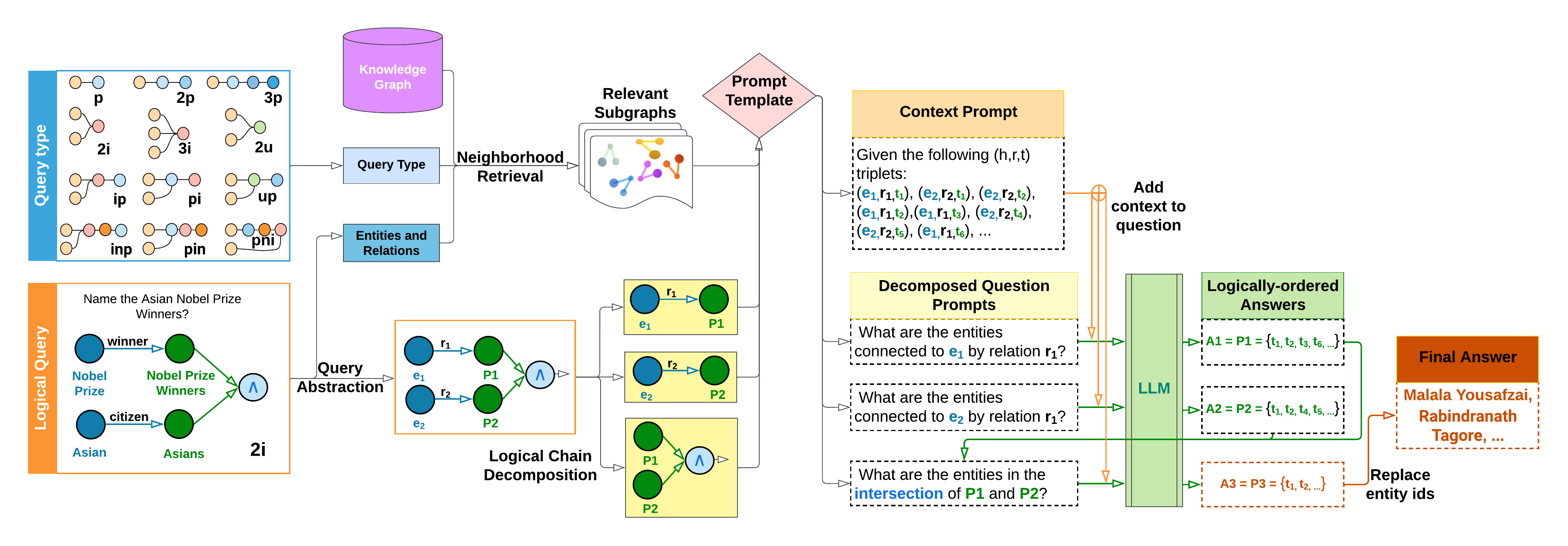## 1 Introduction Knowledge graphs (KGs) encode knowledge in a flexible triplet schema where two entity nodes are connected by relational edges. However, several real-world KGs, such as Freebase (Bollacker et al., 2008), Yago (Suchanek et al., 2007), and NELL (Carlson et al., 2010), are often large-scale, noisy, and incomplete. Thus, reasoning over such KGs is a fundamental and challenging problem in AI research. The over-arching goal of logical reasoning is to develop answering mechanisms for first-order logic (FOL) queries over KGs using the operators of existential quantification ( $\exists$ ), conjunction ( $\wedge$ ), disjunction ( $\vee$ ), and negation ( $\neg$ ). Current research on this topic primarily focuses on the creation of diverse latent space geometries, such as vectors (Hamilton et al., 2018), boxes (Ren et al., 2020), hyperboloids (Choudhary et al., 2021b), and probabilistic distributions (Ren & Leskovec, 2020), in order to effectively capture the semantic position and logical coverage of knowledge graph entities. Despite their success, these approaches are limited in their performance due to the following. (i) Complex queries: They rely on constrained formulations of FOL queries that lose information on complex queries that require chain reasoning (Choudhary et al., 2021a) and involve multiple relationships between entities in the KG, (ii) Generalizability: optimization for a particular KG may not generalize to other KGs which limits the applicability of these approaches in real-world scenarios where KGs can vary widely in terms of their structure and content, and (iii) Scalability: intensive training times that limit the scalability of these approaches to larger KGs and incorporation of new data into existing KGs. To address these limitations, we aim to leverage the reasoning abilities of large language models (LLMs) in a novel framework, shown in Figure 1, called Language-guided Abstract Reasoning over Knowledge graphs (LARK). 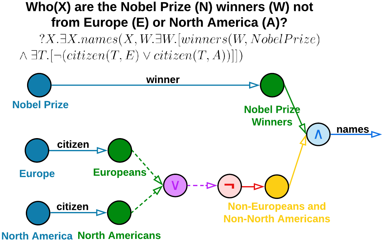<details> <summary>extracted/2305.01157v3/images/example_logical_query.png Details</summary>  ### Visual Description ## Diagram: Logical Structure of Nobel Prize Winners Not from Europe or North America ### Overview The diagram illustrates a logical framework to identify Nobel Prize winners (W) who are not citizens of Europe (E) or North America (A). It uses nodes, arrows, and logical notation to represent relationships between regions, citizenship, and prize-winning status. The central question is: "Who(X) are the Nobel Prize (N) winners (W) not from Europe (E) or North America (A)?" This is formalized in first-order logic at the top of the diagram. --- ### Components/Axes 1. **Nodes**: - **Blue Circles**: Represent regions (Europe, North America). - **Green Circles**: Represent "Europeans" and "Nobel Prize Winners." - **Purple Circle**: Represents the logical variable **V** (likely a placeholder for "not from Europe or North America"). - **Pink Circle**: Labeled "Non-Europeans and Non-North Americans." - **Yellow Circle**: Also labeled "Non-Europeans and Non-North Americans" (duplicate label?). - **Light Blue Circle**: Labeled **Λ** (lambda), connected to "names" via an arrow. 2. **Arrows**: - **Blue Arrows**: Labeled "winner" (connects Nobel Prize to Nobel Prize Winners) and "citizen" (connects regions to their populations). - **Green Arrows**: Labeled "names" (connects Nobel Prize Winners to Λ). - **Red Arrow**: Labeled "¬" (logical negation), connecting V to the pink/yellow node. - **Dashed Green Arrows**: Connect "Europeans" and "North Americans" to V. 3. **Legend**: - **Blue**: Europe. - **Green**: Europeans. - **Purple**: V (logical variable). - **Pink**: Non-Europeans and Non-North Americans. - **Yellow**: Non-Europeans and Non-North Americans (duplicate?). 4. **Logical Formula**: - **Top Text**: "?X.∃X.names(X, W.∃W.[winners(W, NobelPrize) ∧ ∃T.[¬(citizen(T, E) ∨ citizen(T, A))]]])" - Translates to: "There exists an X such that X has names, and there exists a W who is a Nobel Prize winner, and there exists a T who is not a citizen of Europe or North America." --- ### Detailed Analysis 1. **Logical Flow**: - The diagram starts with the question in logical notation, defining the scope of "X" (Nobel Prize winners not from Europe or North America). - Arrows represent relationships: - **Nobel Prize → Nobel Prize Winners**: Winners are associated with the prize. - **Europe/North America → Europeans/North Americans**: Citizenship defines regional populations. - **Europeans/North Americans → V**: Dashed arrows indicate exclusion from the target group (V). - **V → Non-Europeans and Non-North Americans**: Red arrow applies negation to V, defining the target group. - **Nobel Prize Winners → Λ (names)**: Final connection to the names of winners. 2. **Color-Coding**: - Blue (Europe) and green (Europeans) nodes are on the left, connected to V via dashed arrows. - Purple (V) acts as a bridge between regional populations and the excluded group. - Pink/yellow nodes represent the final target group (non-Europeans/non-North Americans). 3. **Ambiguities**: - The yellow and pink nodes share the same label ("Non-Europeans and Non-North Americans"), suggesting a possible redundancy or error. - The role of **Λ (lambda)** is unclear—it may represent a function mapping winners to their names. --- ### Key Observations 1. **Exclusion Logic**: - The diagram uses negation (¬) to exclude citizens of Europe or North America from the target group. - The formula explicitly states: "There exists a T who is not a citizen of Europe or North America." 2. **Redundancy**: - The pink and yellow nodes both label the same group, which may indicate a diagramming error or intentional emphasis. 3. **Logical Structure**: - The use of existential quantifiers (∃) and negation (¬) aligns with formal logic to define the target set. --- ### Interpretation The diagram formalizes a query to identify Nobel Prize winners who are **not citizens of Europe or North America**. It achieves this by: 1. Defining regions (Europe, North America) and their populations (Europeans, North Americans). 2. Using negation to exclude these populations from the target group (V). 3. Connecting Nobel Prize winners to the excluded group via logical operators. The redundancy in labeling (pink/yellow nodes) and the ambiguous role of **Λ** suggest potential gaps in the diagram's design. However, the core logic is clear: the target group consists of Nobel Prize winners whose citizenship does not align with Europe or North America. This could be used to filter winners by geographic origin in a database or dataset. </details> (a) Input logical query. 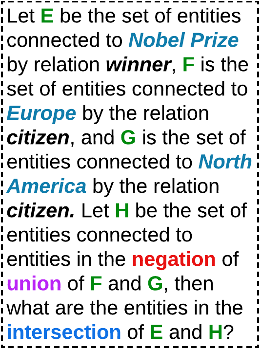<details> <summary>extracted/2305.01157v3/images/example_full_query.png Details</summary>  ### Visual Description ## Text Block: Set Theory Problem ### Overview The image contains a textual problem involving set theory and relations. It defines four sets (E, F, G, H) based on connections to entities via specific relations and asks for the intersection of E and H. Key terms are color-coded for emphasis. ### Components/Axes - **Text Structure**: - **Bold Text**: Highlights key terms (e.g., *winner*, *citizen*, *intersection*). - **Colored Text**: - **Blue**: "Nobel Prize," "Europe," "North America," "intersection." - **Red**: "negation." - **Purple**: "union." - **Green**: Variables **E, F, G, H**. ### Content Details 1. **Set Definitions**: - **E**: Entities connected to *Nobel Prize* via the relation *winner*. - **F**: Entities connected to *Europe* via the relation *citizen*. - **G**: Entities connected to *North America* via the relation *citizen*. - **H**: Entities connected to the *negation of the union of F and G*. 2. **Question**: - What are the entities in the *intersection* of **E** and **H**? ### Key Observations - **Color Coding**: - Blue highlights geographic regions (*Europe*, *North America*) and the final query (*intersection*). - Red emphasizes *negation*, critical to defining **H**. - Purple highlights *union*, which combines **F** and **G** before negation. - **Logical Flow**: - **H** is derived from the complement of the union of **F** and **G** (i.e., entities not in Europe or North America). - The intersection of **E** and **H** seeks Nobel Prize winners who are not citizens of Europe or North America. ### Interpretation - **Set Operations**: - **Union (F ∪ G)**: Combines European and North American citizens. - **Negation (¬(F ∪ G))**: Represents entities outside Europe and North America. - **Intersection (E ∩ H)**: Identifies Nobel Prize winners who are not citizens of Europe or North America. - **Implications**: - The problem tests understanding of set theory operations (union, negation, intersection) and their application to real-world relations (citizenship, awards). - No numerical data is provided; the focus is on logical relationships. ### Notable Patterns - The use of color coding aids in distinguishing regions, operations, and variables. - The problem assumes familiarity with set theory notation and relations. ### Final Answer The entities in the intersection of **E** and **H** are those connected to Nobel Prize winners who are **not** citizens of Europe or North America. </details> (b) Query prompt. 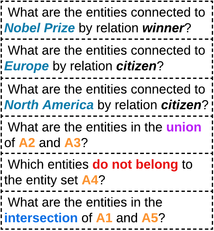<details> <summary>extracted/2305.01157v3/images/example_decomp_query.png Details</summary>  ### Visual Description ## Textual Content Analysis: Entity Relationship Queries ### Overview The image contains six structured questions focused on entity relationships, set operations, and categorical connections. Each question uses colored text to denote specific entities or operations, suggesting a knowledge graph or database query context. ### Components/Axes 1. **Question Structure**: - Format: "What are the entities connected to [Entity] by relation [Relation]?" - Color-coded entities: - `Nobel Prize` (blue) - `Europe` (blue) - `North America` (blue) - `A2` (purple) - `A3` (orange) - `A4` (orange) - `A1` (orange) - `A5` (orange) 2. **Operations**: - Union (`A2` ∪ `A3`) - Exclusion (`do not belong to A4`) - Intersection (`A1` ∩ `A5`) ### Detailed Analysis 1. **Question 1**: - "What are the entities connected to **Nobel Prize** by relation **winner**?" - Focus: Identifying entities that have won the Nobel Prize. 2. **Question 2**: - "What are the entities connected to **Europe** by relation **citizen**?" - Focus: Listing citizens of European countries. 3. **Question 3**: - "What are the entities connected to **North America** by relation **citizen**?" - Focus: Listing citizens of North American countries. 4. **Question 4**: - "What are the entities in the **union** of **A2** and **A3**?" - Focus: Combining entities from sets A2 (purple) and A3 (orange). 5. **Question 5**: - "Which entities **do not belong** to the entity set **A4**?" - Focus: Identifying entities outside set A4 (orange). 6. **Question 6**: - "What are the entities in the **intersection** of **A1** and **A5**?" - Focus: Finding entities common to sets A1 and A5 (both orange). ### Key Observations - **Color Coding**: - Blue text denotes major entities (Nobel Prize, Europe, North America). - Orange/purple text denotes abstract sets (A1–A5), likely representing predefined entity groups. - **Set Operations**: - Union, intersection, and exclusion operations are explicitly tested, indicating a focus on relational logic. - **Geopolitical Scope**: - Questions 2 and 3 anchor the analysis in real-world geography (Europe/North America). ### Interpretation This set of questions appears designed to evaluate understanding of: 1. **Entity-Relation Mapping**: How entities (e.g., people, organizations) connect to broader categories via specific relations (e.g., "winner," "citizen"). 2. **Set Theory Applications**: - Union/Intersection: Combining or finding overlaps between abstract entity sets (A1–A5). - Exclusion: Identifying entities outside a defined set (A4). 3. **Knowledge Graph Queries**: - The structure mirrors SPARQL-like queries for semantic web data, where relations and sets define connections between nodes. The use of colored text suggests a visual or interactive system (e.g., a database interface) where color distinguishes entity types or sets. The absence of numerical data implies a qualitative or categorical analysis focus. </details> (c) Decomposed prompt. 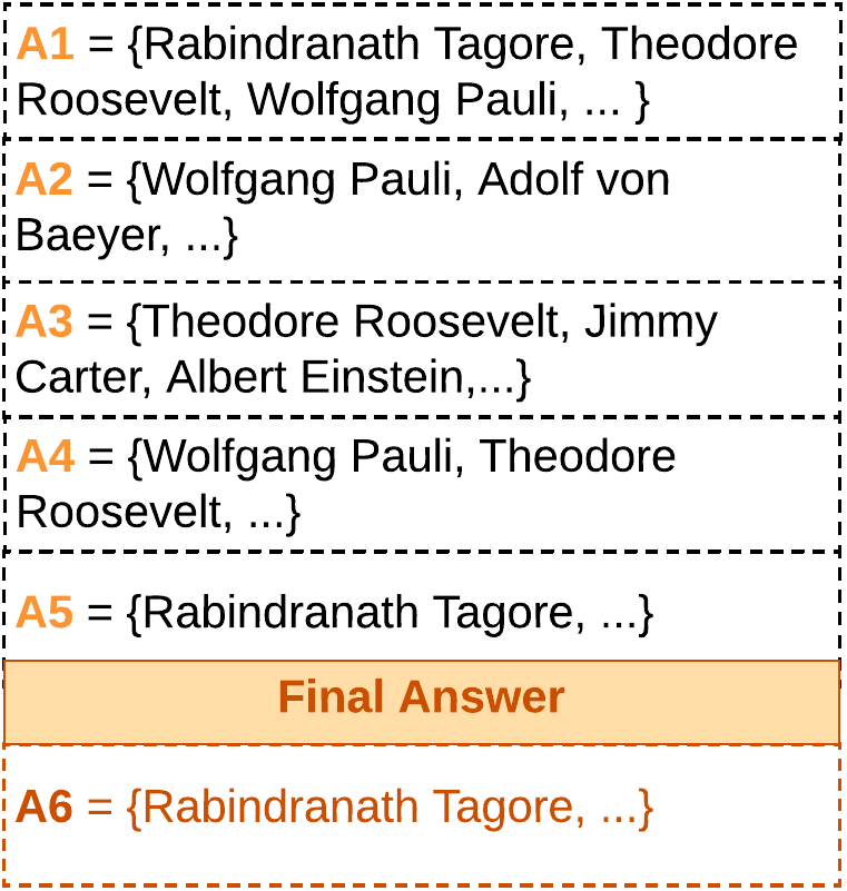<details> <summary>extracted/2305.01157v3/images/example_answers.png Details</summary>  ### Visual Description ## Textual Diagram: Set Intersection Analysis ### Overview The image presents a sequence of six labeled sets (A1–A6) containing names of historical figures. Each set is defined with curly braces and includes three explicitly listed names followed by an ellipsis ("..."), indicating additional unspecified elements. The final answer (A6) is highlighted in orange, suggesting it represents the intersection of all preceding sets. ### Components/Axes - **Labels**: - A1, A2, A3, A4, A5, A6 (set identifiers in orange). - "Final Answer" (highlighted orange box). - **Content Structure**: - Each set contains three named individuals followed by "...". - Names are in black text, with set labels in orange. ### Detailed Analysis 1. **A1**: {Rabindranath Tagore, Theodore Roosevelt, Wolfgang Pauli, ...} 2. **A2**: {Wolfgang Pauli, Adolf von Baeyer, ...} 3. **A3**: {Theodore Roosevelt, Jimmy Carter, Albert Einstein, ...} 4. **A4**: {Wolfgang Pauli, Theodore Roosevelt, ...} 5. **A5**: {Rabindranath Tagore, ...} 6. **A6 (Final Answer)**: {Rabindranath Tagore, ...} ### Key Observations - **Overlap Patterns**: - Wolfgang Pauli appears in A1, A2, and A4. - Theodore Roosevelt appears in A1, A3, and A4. - Rabindranath Tagore appears in A1, A5, and A6. - **Final Answer (A6)**: Contains only Rabindranath Tagore, implying it is the intersection of all sets. - **Ellipsis Usage**: Indicates incomplete listings; exact additional elements are unspecified. ### Interpretation The diagram illustrates a logical progression where each set (A1–A5) contributes to narrowing down the final answer (A6). The repeated inclusion of Rabindranath Tagore across A1, A5, and A6, combined with his exclusive presence in A6, suggests he is the sole common element across all sets. This aligns with the "Final Answer" designation, as intersections in set theory require elements present in every subset. The ellipses imply the sets contain more members, but only the listed names are relevant to the intersection logic. The diagram emphasizes iterative filtering, where overlapping names are progressively eliminated until only Tagore remains. </details> (d) LLM answers. Figure 1: Example of LARK’s query chain decomposition and logically-ordered LLM answering for effective performance. LLMs are more adept at answering simple queries, and hence, we decompose the multi-operation complex logical query (a,b) into elementary queries with single operation (c) and then use a sequential LLM-based answering method to output the final answer (d). In LARK, we utilize the logical queries to search for relevant subgraph contexts over knowledge graphs and perform chain reasoning over these contexts using logically-decomposed LLM prompts. To achieve this, we first abstract out the logical information from both the input query and the KG. Given the invariant nature of logic logical queries follow the same set of rules and procedures irrespective of the KG context., this enables our method to focus on the logical formulation, avoid model hallucination the model ignores semantic common-sense knowledge and infers only from the KG entities for answers., and generalize over different knowledge graphs. From this abstract KG, we extract relevant subgraphs using the entities and relations present in the logical query. These subgraphs serve as context prompts for input to LLMs. In the next phase, we need to effectively handle complex reasoning queries. From previous works (Zhou et al., 2023; Khot et al., 2023), we realize that LLMs are significantly less effective on complex prompts, when compared to a sequence of simpler prompts. Thus to simplify the query, we exploit their logical nature and deterministically decompose the multi-operation query into logically-ordered elementary queries, each containing a single operation (depicted in the transition from Figure 1(b) to 1(c)). Each of these decomposed logical queries is then converted to a prompt and processed through the LLM to generate the final set of answers (shown in Figure 1(d)). The logical queries are handled sequentially, and if query $y$ depends on query $x$ , then $x$ is scheduled before $y$ . Operations are scheduled in a logically-ordered manner to enable batching different logical queries together, and answers are stored in caches for easy access. The proposed approach effectively integrates logical reasoning over knowledge graphs with the capabilities of LLMs, and to the best of our knowledge, is the first of its kind. Unlike previous approaches that rely on constrained formulations of first-order logic (FOL) queries, our approach utilizes logically-decomposed LLM prompts to enable chain reasoning over subgraphs retrieved from knowledge graphs, allowing us to efficiently leverage the reasoning ability of LLMs. Our KG search model is inspired by retrieval-augmented techniques (Chen et al., 2022) but realizes the deterministic nature of knowledge graphs to simplify the retrieval of relevant subgraphs. Moreover, compared to other prompting methods (Wei et al., 2022; Zhou et al., 2023; Khot et al., 2023), our chain decomposition technique enhances the reasoning capabilities in knowledge graphs by leveraging the underlying chain of logical operations in complex queries, and by utilizing preceding answers amidst successive queries in a logically-ordered manner. To summarize, the primary contributions of this paper are as follows: 1. We propose, Language-guided Abstract Reasoning over Knowledge graphs (LARK), a novel model that utilizes the reasoning abilities of large language models to efficiently answer FOL queries over knowledge graphs. 1. Our model uses entities and relations in queries to find pertinent subgraph contexts within abstract knowledge graphs, and then, performs chain reasoning over these contexts using LLM prompts of decomposed logical queries. 1. Our experiments on logical reasoning across standard KG datasets demonstrate that LARK outperforms the previous state-of-the-art approaches by $35\$ MRR on 14 FOL query types based on the operations of projection (p), intersection ( $\wedge$ ), union ( $\vee$ ), and negation ( $\neg$ ). 1. We establish the advantages of chain decomposition by showing that LARK performs $20\$ better on decomposed logical queries when compared to complex queries on the task of logical reasoning. Additionally, our analysis of LLMs shows the significant contribution of increasing scale and better design of underlying LLMs to the performance of LARK. ## 2 Related Work Our work is at the intersection of two topics, namely, logical reasoning over knowledge graphs and reasoning prompt techniques in LLMs. Logical Reasoning over KGs: Initial approaches in this area (Bordes et al., 2013; Nickel et al., 2011; Das et al., 2017; Hamilton et al., 2018) focused on capturing the semantic information of entities and the relational operations involved in the projection between them. However, further research in the area revealed a need for new geometries to encode the spatial and hierarchical information present in the knowledge graphs. To tackle this issue, models such as Query2Box (Ren et al., 2020), HypE (Choudhary et al., 2021b), PERM (Choudhary et al., 2021a), and BetaE (Ren & Leskovec, 2020) encoded the entities and relations as boxes, hyperboloids, Gaussian distributions, and beta distributions, respectively. Additionally, approaches such as CQD (Arakelyan et al., 2021) have focused on improving the performance of complex reasoning tasks through the answer composition of simple intermediate queries. In another line of research, HamQA (Dong et al., 2023) and QA-GNN (Yasunaga et al., 2021) have developed question-answering techniques that use knowledge graph neighborhoods to enhance the overall performance. We notice that previous approaches in this area have focused on enhancing KG representations for logical reasoning. Contrary to these existing methods, our work provides a systematic framework that leverages the reasoning ability of LLMs and tailors them toward the problem of logical reasoning over knowledge graphs. Reasoning prompts in LLMs: Recent studies have shown that LLMs can learn various NLP tasks with just context prompts (Brown et al., 2020). Furthermore, LLMs have been successfully applied to multi-step reasoning tasks by providing intermediate reasoning steps, also known as Chain-of-Thought (Wei et al., 2022; Chowdhery et al., 2022), needed to arrive at an answer. Alternatively, certain studies have composed multiple LLMs or LLMs with symbolic functions to perform multi-step reasoning (Jung et al., 2022; Creswell et al., 2023), with a pre-defined decomposition structure. More recent studies such as least-to-most (Zhou et al., 2023), successive (Dua et al., 2022) and decomposed (Khot et al., 2023) prompting strategies divide a complex prompt into sub-prompts and answer them sequentially for effective performance. While this line of work is close to our approach, they do not utilize previous answers to inform successive queries. LARK is unique due to its ability to utilize logical structure in the chain decomposition mechanism, augmentation of retrieved knowledge graph neighborhood, and multi-phase answering structure that incorporates preceding LLM answers amidst successive queries. ## 3 Methodology In this section, we will describe the problem setup of logical reasoning over knowledge graphs, and describe the various components of our model. ### 3.1 Problem Formulation In this work, we tackle the problem of logical reasoning over knowledge graphs (KGs) $\mathcal{G}:E\times R$ that store entities ( $E$ ) and relations ( $R$ ). Without loss of generality, KGs can also be organized as a set of triplets $\langle e_{1},r,e_{2}\rangle\subseteq\mathcal{G}$ , where each relation $r\in R$ is a Boolean function $r:E\times E\rightarrow\{True,False\}$ that indicates whether the relation $r$ exists between the pair of entities $(e_{1},e_{2})\in E$ . We consider four fundamental first-order logical (FOL) operations: projection (p), intersection ( $\wedge$ ), union ( $\vee$ ), and negation ( $\neg$ ) to query the KG. These operations are defined as follows: $$ \displaystyle q_{p}[Q_{p}] \displaystyle\triangleq?V_{p}:\{v_{1},v_{2},...,v_{k}\}\subseteq E~{}\exists~{ }a_{1} \displaystyle q_{\wedge}[Q_{\wedge}] \displaystyle\triangleq?V_{\wedge}:\{v_{1},v_{2},...,v_{k}\}\subseteq E~{} \exists~{}a_{1}\wedge a_{2}\wedge...\wedge a_{i} \displaystyle q_{\vee}[Q_{\vee}] \displaystyle\triangleq?V_{\vee}:\{v_{1},v_{2},...,v_{k}\}\subseteq E~{} \exists~{}a_{1}\vee a_{2}\vee...\vee a_{i} \displaystyle q_{\neg}[Q_{\neg}] \displaystyle\triangleq?V_{\neg}:\{v_{1},v_{2},...,v_{k}\}\subseteq E~{} \exists~{}\neg a_{1} \displaystyle\text{where }Q_{p},Q_{\neg} \displaystyle=(e_{1},r_{1});~{}Q_{\wedge},Q_{\vee}=\{(e_{1},r_{1}),(e_{2},r_{2 }),...,(e_{i},r_{i})\};\text{~{}~{}and~{} }a_{i}=r_{i}(e_{i},v_{i}) \tag{1} $$ where $q_{p},q_{\wedge},q_{\vee}$ , and $q_{\neg}$ are projection, intersection, union, and negation queries, respectively; and $V_{p},V_{\wedge},V_{\vee}$ and $V_{\neg}$ are the corresponding results of those queries (Arakelyan et al., 2021; Choudhary et al., 2021a). $a_{i}$ is a Boolean indicator which will be 1 if $e_{i}$ is connected to $v_{i}$ by relation $r_{i}$ , 0 otherwise. The goal of logical reasoning is to formulate the operations such that for a given query $q_{\tau}$ of query type $\tau$ with inputs $Q_{\tau}$ , we are able to efficiently retrieve $V_{\tau}$ from entity set $E$ , e.g., for a projection query $q_{p}[\text{(Nobel Prize, winners)}]$ , we want to retrieve $V_{p}=\{\text{Nobel Prize winners}\}\subseteq E$ . In conventional methods for logical reasoning, the query operations were typically expressed through a geometric function. For example, the intersection of queries was represented as an intersection of box representations in Query2Box (Ren et al., 2020). However, in our proposed approach, LARK, we leverage the advanced reasoning capabilities of Language Models (LLMs) and prioritize efficient decomposition of logical chains within the query to enhance performance. This novel strategy seeks to overcome the limitations of traditional methods by harnessing the power of LLMs in reasoning over KGs. ### 3.2 Neighborhood Retrieval and Logical Chain Decomposition The foundation of LARK’s reasoning capability is built on large language models. Nevertheless, the limited input length of LLMs restricts their ability to process the entirety of a knowledge graph. Furthermore, while the set of entities and relations within a knowledge graph is unique, the reasoning behind logical operations remains universal. Therefore, we specifically tailor the LLM prompts to account for the above distinctive characteristics of logical reasoning over knowledge graphs. To address this need, we adopt a two-step process: 1. Query Abstraction: In order to make the process of logical reasoning over knowledge graphs more generalizable to different datasets, we propose to replace all the entities and relations in the knowledge graph and queries with a unique ID. This approach offers three significant advantages. Firstly, it reduces the number of tokens in the query, leading to improved LLM efficiency. Secondly, it allows us to solely utilize the reasoning ability of the language model, without relying on any external common sense knowledge of the underlying LLM. By avoiding the use of common sense knowledge, our approach mitigates the potential for model hallucination (which may lead to the generation of answers that are not supported by the KG). Finally, it removes any KG-specific information, thereby ensuring that the process remains generalizable to different datasets. While this may intuitively seem to result in a loss of information, our empirical findings, presented in Section 4.4, indicate that the impact on the overall performance is negligible. 1. Neighborhood Retrieval: In order to effectively answer logical queries, it is not necessary for the LLM to have access to the entire knowledge graph. Instead, the relevant neighborhoods containing the answers can be identified. Previous approaches (Guu et al., 2020; Chen et al., 2022) have focused on semantic retrieval for web documents. However, we note that logical queries are deterministic in nature, and thus we perform a $k$ -level depth-first traversal where $k$ is determined by the query type, e.g., for 3-level projection ( $3p$ ) queries, $k=3$ . over the entities and relations present in the query. Let $E^{1}_{\tau}$ and $R^{1}_{\tau}$ denote the set of entities and relations in query $Q_{\tau}$ for a query type $\tau$ , respectively. Then, the $k$ -level neighborhood of query $q_{\tau}$ is defined by $\mathcal{N}_{k}(q_{\tau}[Q_{\tau}])$ as: $$ \displaystyle\mathcal{N}_{1}(q_{\tau}[Q_{\tau}]) \displaystyle=\left\{(h,r,t):\left(h\in E^{1}_{\tau}\right),\left(r\in R^{1}_{ \tau}\right),\left(t\in E^{1}_{\tau}\right)\right\} \displaystyle E^{k}_{\tau} \displaystyle=\{h,t:(h,r,t)\in\mathcal{N}_{k-1}(q_{\tau}[Q_{\tau}]\},\quad R^{ k}_{\tau}=\{r:(h,r,t)\in\mathcal{N}_{k-1}(q_{\tau}[Q_{\tau}]\} \displaystyle\mathcal{N}_{k}(q_{\tau}[Q_{\tau}]) \displaystyle=\left\{(h,r,t):\left(h\in E^{k}_{\tau}\right),\left(r\in R^{k}_{ \tau}\right),\left(t\in E^{k}_{\tau}\right)\right\} \tag{5} $$ We have taken steps to make our approach more generalizable and efficient by abstracting the query and limiting input context for LLMs. However, the complexity of a query still remains a concern. The complexity of a query type $\tau$ , denoted by $\mathcal{O}(q_{\tau})$ , is determined by the number of entities and relations it involves, i.e., $\mathcal{O}(q_{\tau})\propto|E_{\tau}|+|R_{\tau}|$ . In other words, the size of the query in terms of its constituent elements is a key factor in determining its computational complexity. This observation is particularly relevant in the context of LLMs, as previous studies have shown that their performance tends to decrease as the complexity of the queries they handle increases (Khot et al., 2023). To address this, we propose a logical query chain decomposition mechanism in LARK which reduces a complex multi-operation query to multiple single-operation queries. Due to the exhaustive set of operations, we apply the following strategy for decomposing the various query types: - Reduce a $k$ -level projection query to $k$ one-level projection queries, e.g., a $3p$ query with one entity and three relations $e_{1}\xrightarrow{r_{1}}\xrightarrow{r_{2}}\xrightarrow{r_{3}}A$ is decomposed to $e_{1}\xrightarrow{r_{1}}A_{1},A_{1}\xrightarrow{r_{2}}A_{2},A_{2}\xrightarrow{ r_{3}}A$ . - Reduce a $k$ -intersection query to $k$ projection queries and an intersection query, e.g., a $3i$ query with intersection of two projection queries $(e_{1}\xrightarrow{r_{1}})\wedge(e_{2}\xrightarrow{r_{2}})\wedge(e_{3} \xrightarrow{r_{3}})=A$ is decomposed to $e_{1}\xrightarrow{r_{1}}A_{1},e_{2}\xrightarrow{r_{2}}A_{2},e_{3}\xrightarrow{ r_{3}}A_{2},A_{1}\wedge A_{2}\wedge A_{3}=A$ . Similarly, reduce a $k$ -union query to $k$ projection queries and a union query. The complete decomposition of the exhaustive set of query types used in previous work (Ren & Leskovec, 2020) and our empirical studies can be found in Appendix A. <details> <summary>extracted/2305.01157v3/images/model.png Details</summary>  ### Visual Description ## Flowchart: Knowledge Graph Query Processing System ### Overview The diagram illustrates a multi-stage pipeline for processing complex queries using knowledge graphs and logical decomposition. It begins with query abstraction, progresses through subgraph retrieval and prompt engineering, and culminates in LLM-based answer synthesis. The final output combines entity-level reasoning with contextual knowledge to produce human-readable answers. ### Components/Axes 1. **Left Panel (Query Abstraction)** - **Query Type Matrix**: - Contains 9 query patterns (2p, 3p, 2i, ip, pi, up, inp, pin, pini) - Color-coded nodes (blue, green, orange) representing entity types - **Logical Query Example**: - "Name the Asian Nobel Prize Winners?" - Visualized with entity-relationship graph (Asian → winner → Nobel Prize) 2. **Central Processing Flow** - **Knowledge Graph** (purple cylinder) - **Neighborhood Retrieval** (blue box) - **Relevant Subgraphs** (wavy-edged box with colored nodes) - **Prompt Template** (pink diamond) 3. **Right Panel (LLM Processing)** - **Context Prompt** (orange box with triplet examples) - **Decomposed Question Prompts** (yellow box with 3 sub-questions) - **LLM Processing** (green vertical box) - **Logically-ordered Answers** (green dashed boxes with A1-A3) - **Final Answer** (orange box with Malala Yousafzai, Rabindranath Tagore) ### Detailed Analysis 1. **Query Type System** - 9 distinct query patterns categorized by: - Node count (2p=2 nodes, 3p=3 nodes) - Relationship types (p=property, i=instance) - Special cases (inp=inverse property, pin=inverse with negation) 2. **Knowledge Graph Integration** - Central data source represented as a purple cylinder - Connected to query abstraction and neighborhood retrieval 3. **Logical Decomposition** - Original query broken into 3 sub-questions: 1. Entities connected to e₁ by r₁ 2. Entities connected to e₂ by r₂ 3. Intersection of P1 and P2 entity sets 4. **LLM Processing** - Takes decomposed prompts and generates: - A1 = {t₁, t₂, t₃, t₆...} (entities for P1) - A2 = {t₁, t₂, t₄, t₅...} (entities for P2) - A3 = {t₁, t₂...} (intersection set) 5. **Answer Synthesis** - Final answer combines entity IDs with real-world names - Example output: "Malala Yousafzai, Rabindranath Tagore..." ### Key Observations 1. **Hierarchical Processing**: - Query abstraction → subgraph retrieval → prompt engineering → LLM processing → answer synthesis 2. **Entity-Relationship Focus**: - All stages maintain explicit connections between entities (e₁, e₂) and relations (r₁, r₂) 3. **Temporal Logic**: - Intersection operation (A3) suggests temporal or logical dependency between sub-answers 4. **Contextual Enrichment**: - Triplets in context prompt provide background knowledge for answer interpretation ### Interpretation This system demonstrates a sophisticated approach to knowledge graph querying that: 1. **Handles Complexity**: Breaks down multi-hop queries into manageable components 2. **Leverages LLM Capabilities**: Uses large language models for contextual understanding and answer synthesis 3. **Maintains Logical Consistency**: Ensures answers respect original query constraints through decomposition and intersection operations 4. **Bridges Formal and Natural Language**: Converts formal entity-relationship representations into human-readable names The process reveals an intentional design to handle both the structural complexity of knowledge graphs and the semantic nuances required for accurate answer generation. The use of color-coded nodes and explicit decomposition steps suggests a focus on making the reasoning process transparent and verifiable. </details> Figure 2: An overview of the LARK model. The model takes the logical query and infers the query type from it. The query abstraction function maps the entities and relations to abstract IDs, and the neighborhood retrieval mechanism collects the relevant subgraphs from the overall knowledge graph. The chains of the abstracted complex query are then logically decomposed to simpler single-operation queries. The retrieved neighborhood and decomposed queries are further converted into LLM prompts using a template and then processed in the LLM to get the final set of answers for evaluation. ### 3.3 Chain Reasoning Prompts In the previous section, we outlined our approach to limit the neighborhood and decompose complex queries into chains of simple queries. Leveraging these, we can now use the reasoning capability of LLMs to obtain the final set of answers for the query, as shown in Figure 2. To achieve this, we employ a prompt template that converts the neighborhood into a context prompt and the decomposed queries into question prompts. It is worth noting that certain queries in the decomposition depend on the responses of preceding queries, such as intersection relying on the preceding projection queries. Additionally, unlike previous prompting methods such as chain-of-thought (Wei et al., 2022) and decomposition (Khot et al., 2023) prompting, the answers need to be integrated at a certain position in the prompt. To address this issue, we maintain a placeholder in dependent queries and a temporary cache of preceding answers that can replace the placeholders in real-time. This also has the added benefit of maintaining the parallelizability of queries, as we can run batches of decomposed queries in phases instead of sequentially running each decomposed query. The specific prompt templates of the complex and decomposed logical queries for different query types are provided in Appendix B. ### 3.4 Implementation Details We implemented LARK in Pytorch (Paszke et al., 2019) on eight Nvidia A100 GPUs with 40 GB VRAM. In the case of LLMs, we chose the Llama2 model (Touvron et al., 2023) due to its public availability in the Huggingface library (Wolf et al., 2020) . For efficient inference over the large-scale models, we relied on the mixed-precision version of LLMs and the Deepspeed library (Rasley et al., 2020) with Zero stage 3 optimization. The algorithm of our model is provided in Appendix D and implementation code for all our experiments with exact configuration files and datasets for reproducibility are publicly available https://github.com/Akirato/LLM-KG-Reasoning. In our experiments, the highest complexity of a query required a 3-hop neighborhood around the entities and relations. Hence, we set the depth limit to 3 (i.e., $k=3$ ). Additionally, to further make our process completely compatible with different datasets, we added a limit of $n$ tokens on the input which is dependent on the LLM model (for Llama2, $n$ =4096). In practice, this implies that we stop the depth-first traversal when the context becomes longer than $n$ . ## 4 Experimental Results This sections describes our experiments that aim to answer the following research questions (RQs): - Does LARK outperform the state-of-the-art baselines on the task of logical reasoning over standard knowledge graph benchmarks? - How does our combination of chain decomposition query and logically-ordered answer mechanism perform in comparison with the standard prompting techniques? - How does the scale and design of LARK’s underlying LLM model affect its performance? - How would our model perform with support for increased token size? - Does query abstraction affect the reasoning performance of our model? ### 4.1 Datasets and Baselines We select the following standard benchmark datasets to investigate the performance of our model against state-of-the-art models on the task of logical reasoning over knowledge graphs: - FB15k (Bollacker et al., 2008) is based on Freebase, a large collaborative knowledge graph project that was created by Google. FB15k contains about 15,000 entities, 1,345 relations, and 592,213 triplets (statements that assert a fact about an entity). - FB15k-237 (Toutanova et al., 2015) is a subset of FB15k, containing 14,541 entities, 237 relations, and 310,116 triplets. The relations in FB15k-237 are a subset of the relations in FB15k, and was created to address some of the limitations of FB15k, such as the presence of many irrelevant or ambiguous relations, and to provide a more challenging benchmark for knowledge graph completion models. - NELL995 (Carlson et al., 2010) was created using the Never-Ending Language Learning (NELL) system, which is a machine learning system that automatically extracts knowledge from the web by reading text and inferring new facts. NELL995 contains 9,959 entities, 200 relations, and 114,934 triplets. The relations in NELL995 cover a wide range of domains, including geography, sports, and politics. Our criteria for selecting the above datasets was their ubiquity in previous works on this research problem. Further details on their token size is provided in Appendix E. For the baselines, we chose the following methods: - GQE (Hamilton et al., 2018) encodes a query as a single vector and represents entities and relations in a low-dimensional space. It uses translation and deep set operators, which are modeled as projection and intersection operators, respectively. - Query2Box (Q2B) (Ren et al., 2020) uses a box embedding model which is a generalization of the traditional vector embedding model and can capture richer semantics. - BetaE (Ren & Leskovec, 2020) uses a novel beta distribution to model the uncertainty in the representation of entities and relations. BetaE can capture both the point estimate and the uncertainty of the embeddings, which leads to more accurate predictions in knowledge graph completion tasks. - HQE (Choudhary et al., 2021b) uses the hyperbolic query embedding mechanism to model the complex queries in knowledge graph completion tasks. - HypE (Choudhary et al., 2021b) uses the hyperboloid model to represent entities and relations in a knowledge graph that simultaneously captures their semantic, spatial, and hierarchical features. - CQD (Arakelyan et al., 2021) decomposes complex queries into simpler sub-queries and applies a query-specific attention mechanism to the sub-queries. ### 4.2 RQ1. Efficacy on Logical Reasoning To study the efficacy of our model on the task of logical reasoning, we compare it against the previous baselines on the following standard logical query constructs: 1. Multi-hop Projection traverses multiple relations from a head entity in a knowledge graph to answer complex queries by projecting the query onto the target entities. In our experiments, we consider $1p,2p$ , and $3p$ queries that denote 1-relation, 2-relation, and 3-relation hop from the head entity, respectively. 1. Geometric Operations apply the operations of intersection ( $\wedge$ ) and union ( $\vee$ ) to answer the query. Our experiments use $2i$ and $3i$ queries that represent the intersection over 2 and 3 entities, respectively. Also, we study $2u$ queries that perform union over 2 entities. 1. Compound Operations integrate multiple operations such as intersection, union, and projection to handle complex queries over a knowledge graph. 1. Negation Operations negate the query by finding entities that do not satisfy the given logic. In our experiments, we examine $2in,3in,inp,$ and $pin$ queries that negate $2i,3i,ip,$ and $pi$ queries, respectively. We also analyze $pni$ (an additional variant of the $pi$ query), where the negation is over both entities in the intersection. It should be noted that BetaE is the only method in the existing literature that supports negation, and hence, we only compare against it in our experiments. We present the results of our experimental study, which compares the Mean Reciprocal Rank (MRR) score of the retrieved candidate entities using different query constructions. MRR is calculated as the average of the reciprocal ranks of the candidate entities More metrics such as HITS@K=1,3,10 are reported in Appendix C.. In order to ensure a fair comparison, We selected these query constructions which were used in most of the previous works in this domain (Ren & Leskovec, 2020). An illustration of these query types is provided in Appendix A for better understanding. Our experiments show that LARK outperforms previous state-of-the-art baselines by $35\$ on an average across different query types, as reported in Table 1. We observe that the performance improvement is higher for simpler queries, where $1p>2p>3p$ and $2i>3i$ . This suggests that LLMs are better at capturing breadth across relations but may not be as effective at capturing depth over multiple relations. Moreover, our evaluation also encompasses testing against challenging negation queries, for which BetaE (Ren & Leskovec, 2020) remains to be the only existing approach. Even in this complex scenario, our findings, as illustrated in Table 2, indicate that LARK significantly outperforms the baselines by $140\$ . This affirms the superior reasoning capabilities of our model in tackling complex query scenarios. Another point of note is that certain baselines such as CQD are able to outperform LARK in the FB15k dataset for certain query types such as $1p,3i$ , and $ip$ . The reason for this is that FB15k suffers from a data leakage from training to validation and testing sets (Toutanova et al., 2015). This unfairly benefits the training-based baselines over the inference-only LARK model. Table 1: Performance comparison between LARK and the baseline in terms of their efficacy of logical reasoning using MRR scores. The rows present various models and the columns correspond to different query structures of multi-hop projections, geometric operations, and compound operations. The best results for each query type in every dataset is highlighted in bold font. | FB15k | GQE Q2B BetaE | 54.6 68.0 65.1 | 15.3 21.0 25.7 | 10.8 14.2 24.7 | 39.7 55.1 55.8 | 51.4 66.5 66.5 | 27.6 39.4 43.9 | 19.1 26.1 28.1 | 22.1 35.1 40.1 | 11.6 16.7 25.2 | | --- | --- | --- | --- | --- | --- | --- | --- | --- | --- | --- | | HQE | 54.3 | 33.9 | 23.3 | 38.4 | 50.6 | 12.5 | 24.9 | 35.0 | 25.9 | | | HypE | 67.3 | 43.9 | 33.0 | 49.5 | 61.7 | 18.9 | 34.7 | 47.0 | 37.4 | | | CQD | 79.4 | 39.6 | 27.0 | 74.0 | 78.2 | 70.0 | 43.3 | 48.4 | 17.5 | | | LARK(complex) | 73.6 | 46.5 | 32.0 | 66.9 | 61.8 | 24.8 | 47.2 | 47.7 | 37.5 | | | LARK(ours) | 73.6 | 49.3 | 35.1 | 67.8 | 62.6 | 29.3 | 54.5 | 51.9 | 37.7 | | | FB15k-237 | GQE | 35.0 | 7.2 | 5.3 | 23.3 | 34.6 | 16.5 | 10.7 | 8.2 | 5.7 | | Q2B | 40.6 | 9.4 | 6.8 | 29.5 | 42.3 | 21.2 | 12.6 | 11.3 | 7.6 | | | BetaE | 39.0 | 10.9 | 10.0 | 28.8 | 42.5 | 22.4 | 12.6 | 12.4 | 9.7 | | | HQE | 37.6 | 20.9 | 16.9 | 25.3 | 35.2 | 17.3 | 8.2 | 15.6 | 17.9 | | | HypE | 49.0 | 34.3 | 23.7 | 33.9 | 44 | 18.6 | 30.5 | 41.0 | 26.0 | | | CQD | 44.5 | 11.3 | 8.1 | 32.0 | 42.7 | 25.3 | 15.3 | 13.4 | 4.8 | | | LARK(complex) | 70.0 | 34.0 | 21.5 | 43.4 | 42.2 | 18.7 | 38.4 | 49.2 | 25.1 | | | LARK(ours) | 70.0 | 36.9 | 24.5 | 44.3 | 43.1 | 23.2 | 45.6 | 56.6 | 25.4 | | | NELL995 | GQE | 32.8 | 11.9 | 9.6 | 27.5 | 35.2 | 18.4 | 14.4 | 8.5 | 8.8 | | Q2B | 42.2 | 14.0 | 11.2 | 33.3 | 44.5 | 22.4 | 16.8 | 11.3 | 10.3 | | | BetaE | 53.0 | 13.0 | 11.4 | 37.6 | 47.5 | 24.1 | 14.3 | 12.2 | 8.5 | | | HQE | 35.5 | 20.9 | 18.9 | 23.2 | 36.3 | 8.8 | 13.7 | 21.3 | 15.5 | | | HypE | 46.0 | 30.6 | 27.9 | 33.6 | 48.6 | 31.8 | 13.5 | 20.7 | 26.4 | | | CQD | 50.7 | 18.4 | 13.8 | 39.8 | 49.0 | 29.0 | 22.0 | 16.3 | 9.9 | | | LARK(complex) | 83.2 | 39.8 | 27.6 | 49.3 | 48.0 | 18.7 | 19.6 | 8.3 | 36.8 | | | LARK(ours) | 83.2 | 42.3 | 31.0 | 49.9 | 48.7 | 23.1 | 23.0 | 20.1 | 37.2 | | Table 2: Performance comparison between LARK and the baseline for negation query types using MRR scores. The best results for each query type in every dataset is highlighted in bold font. Our model’s performance is significantly higher on most negation queries. However, the performance is limited in 3in and pni queries due to their high number of tokens (shown in Appendix E). | FB15k | BetaE LARK(complex) LARK(ours) | 14.3 16.5 17.5 | 14.7 6.2 7.0 | 11.5 32.5 34.7 | 6.5 22.8 26.7 | 12.4 10.5 11.1 | | --- | --- | --- | --- | --- | --- | --- | | FB15k-237 | BetaE | 5.1 | 7.9 | 7.4 | 3.6 | 3.4 | | LARK(complex) | 6.1 | 3.4 | 21.6 | 12.8 | 2.9 | | | LARK(ours) | 7.0 | 4.1 | 23.9 | 16.8 | 3.5 | | | NELL995 | BetaE | 5.1 | 7.8 | 10.0 | 3.1 | 3.5 | | LARK(complex) | 8.9 | 5.3 | 23.0 | 10.4 | 6.3 | | | LARK(ours) | 10.4 | 6.6 | 25.4 | 13.6 | 7.6 | | ### 4.3 RQ2. Advantages of Chain Decomposition The aim of this experiment is to investigate the advantages of using chain decomposed queries over standard complex queries. We employ the same experimental setup described in Section 4.2. Our results, in Tables 1 and 2, demonstrate that utilizing chain decomposition contributes to a significant improvement of $20\$ in our model’s performance. This improvement is a clear indication of the LLMs’ ability to capture a broad range of relations and effectively utilize this capability for enhancing the performance on complex queries. This study highlights the potential of using chain decomposition to overcome the limitations of complex queries and improve the efficiency of logical reasoning tasks. This finding is a significant contribution to the field of natural language processing and has implications for various other applications such as question-answering systems and knowledge graph completion. Overall, our results suggest that chain-decomposed queries could be a promising approach for improving the performance of LLMs on complex logical reasoning tasks. ### 4.4 RQ3. Analysis of LLM scale This experiment analyzes the impact of the size of the underlying LLMs and query abstraction on the overall LARK model performance. To examine the effect of LLM size, we compared two variants of the Llama2 model which have 7 billion and 13 billion parameters. Our evaluation results, presented in Table 3, show that the performance of the LARK model improves by $123\$ from Llama2-7B to Llama2-13B. This indicates that increasing the number of LLM parameters can enhance the performance of LARK model. Table 3: MRR scores of LARK on FB15k-237 dataset with underlying LLMs of different sizes. The best results for each query type is highlighted in bold font. | Llama2 | 7B | 73.1 | 33.2 | 20.6 | 10.6 | 25.2 | 25.9 | 17.2 | 20.8 | 24.3 | 4 | 1.8 | 14.2 | 7.4 | 1.9 | | --- | --- | --- | --- | --- | --- | --- | --- | --- | --- | --- | --- | --- | --- | --- | --- | | 13B | 73.6 | 49.3 | 35.1 | 67.8 | 62.6 | 29.3 | 54.5 | 51.9 | 37.7 | 7.0 | 4.1 | 23.9 | 16.8 | 3.5 | | ### 4.5 RQ4. Study on Increased Token Limit of LLMs From the dataset details provided in Appendix E, we observe that the token size of different query types shows considerable fluctuation from $58$ to over $100,000$ . Unfortunately, the token limit of LLama2, considered as the base in our experiments, is 4096. This limit is insufficient to demonstrate the full potential performance of LARK on our tasks. To address this limitation, we consider the availability of models with higher token limits, such as GPT-3.5 (OpenAI, 2023). However, we acknowledge that these models are expensive to run and thus, we could not conduct a thorough analysis on the entire dataset. Nevertheless, to gain insight into LARK’s potential with increased token size, we randomly sampled 1000 queries per query type from each dataset with token length over 4096 and less than 4096 and compared our model on these queries with GPT-3.5 and Llama2 as the base. The evaluation results, which are displayed in Table 4, demonstrate that transitioning from Llama2 to GPT-3.5 can lead to a significant performance improvement of 29%-40% for the LARK model which suggests that increasing the token limit of LLMs may have significant potential of further performance enhancement. Table 4: MRR scores of LARK with Llama2 and GPT LLMs as the underlying base models. The best results for each query type in every dataset is highlighted in bold font. | | FB15k | | | | | | | | | | | | | | | --- | --- | --- | --- | --- | --- | --- | --- | --- | --- | --- | --- | --- | --- | --- | | LLM | 1p | 2p | 3p | 2i | 3i | ip | pi | 2u | up | 2in | 3in | inp | pin | pni | | Llama2-7B | 23.4 | 21.5 | 22.6 | 3.4 | 3 | 26.1 | 18.4 | 14.8 | 3.9 | 9.5 | 4.7 | 21.7 | 26.4 | 5.8 | | Llama2-13B | 23.8 | 22.8 | 24.2 | 3.5 | 3 | 23.3 | 30.8 | 30.7 | 3.9 | 12.4 | 6.6 | 28.4 | 51.4 | 7.7 | | GPT-3.5 | 36.1 | 34.6 | 36.8 | 17.0 | 14.4 | 35.4 | 46.7 | 39.3 | 19.5 | 18.8 | 10.0 | 43.1 | 56.7 | 11.6 | | FB15k-237 | | | | | | | | | | | | | | | | LLM | 1p | 2p | 3p | 2i | 3i | ip | pi | 2u | up | 2in | 3in | inp | pin | pni | | Llama2-7B | 23.1 | 27.4 | 31.5 | 5 | 4.1 | 26.6 | 20.9 | 15.3 | 5.6 | 26.6 | 8.8 | 33.7 | 31 | 21.1 | | Llama2-13B | 23.5 | 29.2 | 33.8 | 5 | 4.1 | 23.7 | 35 | 31.7 | 5.6 | 34.7 | 12.3 | 44 | 60.4 | 28 | | GPT-3.5 | 35.7 | 44.2 | 51.2 | 24.8 | 20.2 | 36.0 | 53.1 | 40.6 | 28.1 | 52.5 | 18.7 | 66.8 | 66.6 | 42.4 | | NELL995 | | | | | | | | | | | | | | | | LLM | 1p | 2p | 3p | 2i | 3i | ip | pi | 2u | up | 2in | 3in | inp | pin | pni | | Llama2-7B | 28 | 24.4 | 27.6 | 3.7 | 3.2 | 24 | 8.4 | 14.5 | 5.7 | 14 | 7.7 | 23.1 | 21.3 | 13.4 | | Llama2-13B | 28.4 | 26 | 29.5 | 3.7 | 3.2 | 21.5 | 14.1 | 25.4 | 5.7 | 18.3 | 10.8 | 30.1 | 30.2 | 17.7 | | GPT-3.5 | 43.1 | 39.4 | 44.8 | 18.3 | 15.5 | 32.6 | 21.4 | 38.5 | 28.3 | 27.7 | 16.4 | 45.7 | 45.9 | 26.8 | ### 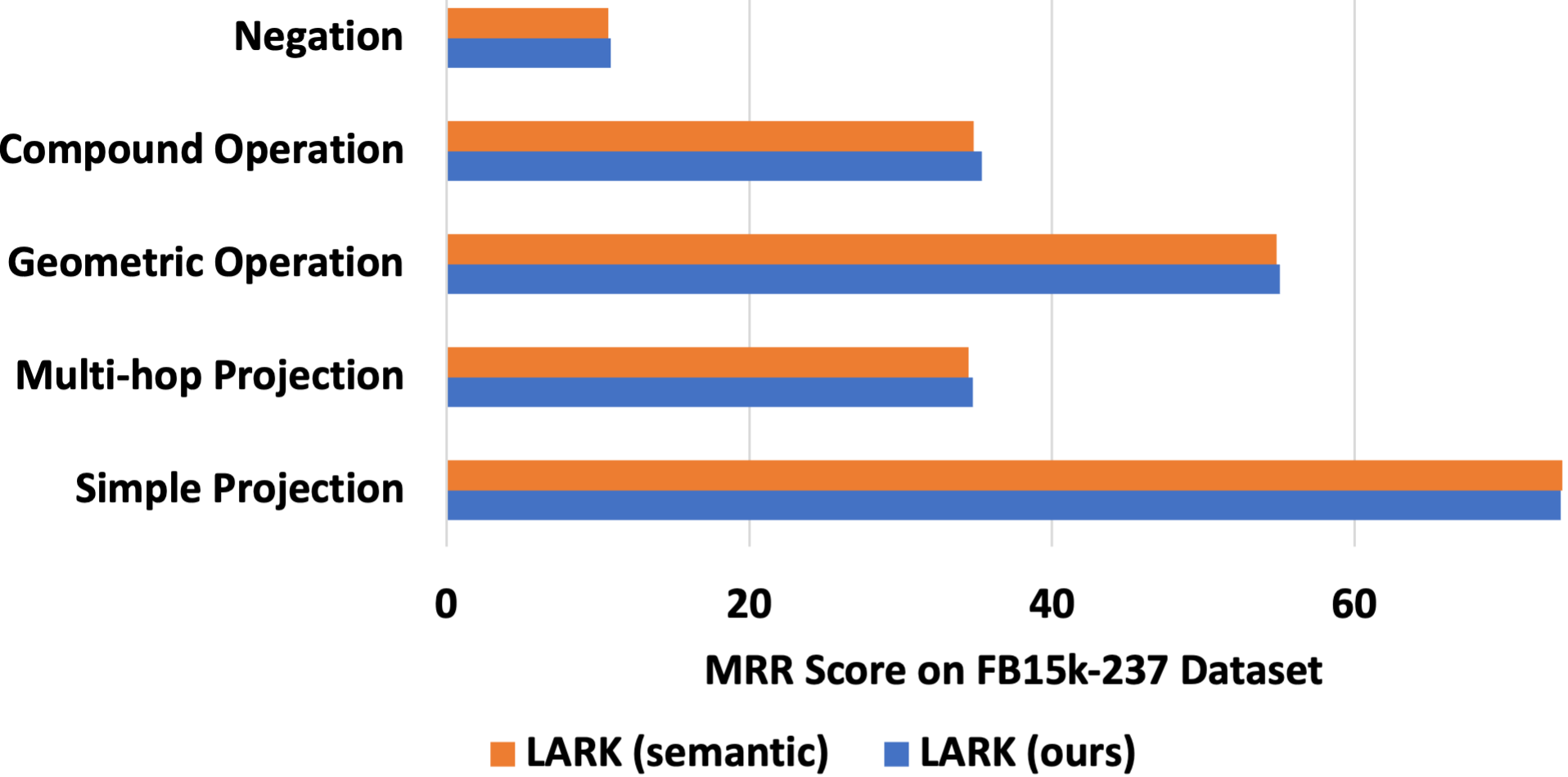4.6 RQ5. Effects of Query Abstraction <details> <summary>extracted/2305.01157v3/images/query_abstraction.png Details</summary>  ### Visual Description ## Bar Chart: MRR Score on FB15k-237 Dataset ### Overview The chart compares the Mean Reciprocal Rank (MRR) scores of two versions of the LARK model ("LARK (semantic)" and "LARK (ours)") across five operations on the FB15k-237 dataset. The x-axis represents MRR scores (0–70), and the y-axis lists the operations: Negation, Compound Operation, Geometric Operation, Multi-hop Projection, and Simple Projection. ### Components/Axes - **X-axis**: MRR Score (0–70, linear scale). - **Y-axis**: Operations (categorical, ordered from top to bottom: Negation, Compound Operation, Geometric Operation, Multi-hop Projection, Simple Projection). - **Legend**: - Orange: LARK (semantic) - Blue: LARK (ours) - **Title**: "MRR Score on FB15k-237 Dataset" (centered above the chart). ### Detailed Analysis 1. **Negation**: - Both versions score ~10 MRR. - Blue (ours) slightly exceeds orange (semantic) by ~0.5. 2. **Compound Operation**: - Both versions score ~35 MRR. - Blue (ours) marginally higher (~35.5 vs. ~35). 3. **Geometric Operation**: - Both versions score ~55 MRR. - Blue (ours) slightly higher (~55.5 vs. ~55). 4. **Multi-hop Projection**: - Orange (semantic): ~34 MRR. - Blue (ours): ~34.5 MRR. 5. **Simple Projection**: - Both versions score ~70 MRR. - Blue (ours) marginally higher (~70.5 vs. ~70). ### Key Observations - **Highest Performance**: Simple Projection dominates all operations with ~70 MRR. - **Consistency**: LARK (ours) consistently outperforms LARK (semantic) by small margins (~0.5–1 MRR) across all operations except Negation. - **Lowest Performance**: Negation scores the lowest (~10 MRR) for both versions. ### Interpretation The chart demonstrates that the "LARK (ours)" version achieves marginally better performance than "LARK (semantic)" across most operations, with the largest relative improvement in Multi-hop Projection. The near-identical scores in Simple Projection suggest both versions excel at this task, but "ours" retains a slight edge. The minimal differences imply that the modifications in "LARK (ours)" may optimize specific operations without drastically altering overall performance. The consistent gap highlights the importance of fine-tuning for task-specific improvements. </details> Figure 3: Effects of Query Abstraction. Regarding the analysis of query abstraction, we considered a variant of LARK called ‘LARK (semantic)’, which retains semantic information in KG entities and relations. As shown in Figure 3, we observe that semantic information provides a minor performance enhancement of $0.01\$ for simple projection queries. However, in more complex queries, it results in a performance degradation of $0.7\$ . The primary cause of this degradation is that the inclusion of semantic information exceeds the LLMs’ token limit, leading to a loss of neighborhood information. Hence, we assert that query abstraction is not only a valuable technique for mitigating model hallucination and achieving generalization across different KG datasets but can also enhance performance by reducing token size. ## 5 Concluding Discussion In this paper, we presented LARK, the first approach to integrate logical reasoning over knowledge graphs with the capabilities of LLMs. Our approach utilizes logically-decomposed LLM prompts to enable chain reasoning over subgraphs retrieved from knowledge graphs, allowing us to efficiently leverage the reasoning ability of LLMs. Through our experiments on logical reasoning across standard KG datasets, we demonstrated that LARK outperforms previous state-of-the-art approaches by a significant margin on 14 different FOL query types. Finally, our work also showed that the performance of LARK improves with increasing scale and better design of the underlying LLMs. We demonstrated that LLMs that can handle larger input token lengths can lead to significant performance improvements. Overall, our approach presents a promising direction for integrating LLMs with logical reasoning over knowledge graphs. The proposed approach of using LLMs for complex logical reasoning over KGs is expected to pave a new way for improved reasoning over large, noisy, and incomplete real-world KGs. This can potentially have a significant impact on various applications such as natural language understanding, question answering systems, intelligent information retrieval systems, etc. For example, in healthcare, KGs can be used to represent patient data, medical knowledge, and clinical research, and logical reasoning over these KGs can enable better diagnosis, treatment, and drug discovery. However, there can also be some ethical considerations that can be taken into account. As with most of the AI-based technologies, there is a potential risk of inducing bias into the model, which can lead to unfair decisions and actions. Bias can be introduced in the KGs themselves, as they are often created semi-automatically from biased sources, and can be amplified by the logical reasoning process. Moreover, the large amount of data used to train LLMs can also introduce bias, as it may reflect societal prejudices and stereotypes. Therefore, it is essential to carefully monitor and evaluate the KGs and LLMs used in this approach to ensure fairness and avoid discrimination. The performance of this method is also dependent on the quality and completeness of the KGs used, and the limited token size of current LLMs. But, we also observe that the current trend of increasing LLM token limits will soon resolve some of these limitations. ## References - Arakelyan et al. (2021) Erik Arakelyan, Daniel Daza, Pasquale Minervini, and Michael Cochez. Complex query answering with neural link predictors. In International Conference on Learning Representations, 2021. URL https://openreview.net/forum?id=Mos9F9kDwkz. - Bollacker et al. (2008) Kurt Bollacker, Colin Evans, Praveen Paritosh, Tim Sturge, and Jamie Taylor. Freebase: A collaboratively created graph database for structuring human knowledge. In Proceedings of the 2008 ACM SIGMOD International Conference on Management of Data, SIGMOD ’08, pp. 1247–1250, New York, NY, USA, 2008. Association for Computing Machinery. URL https://doi.org/10.1145/1376616.1376746. - Bordes et al. (2013) Antoine Bordes, Nicolas Usunier, Alberto Garcia-Duran, Jason Weston, and Oksana Yakhnenko. Translating embeddings for modeling multi-relational data. In C.J. Burges, L. Bottou, M. Welling, Z. Ghahramani, and K.Q. Weinberger (eds.), Advances in Neural Information Processing Systems, volume 26. Curran Associates, Inc., 2013. URL https://proceedings.neurips.cc/paper_files/paper/2013/file/1cecc7a77928ca8133fa24680a88d2f9-Paper.pdf. - Brown et al. (2020) Tom Brown, Benjamin Mann, Nick Ryder, Melanie Subbiah, Jared D Kaplan, Prafulla Dhariwal, Arvind Neelakantan, Pranav Shyam, Girish Sastry, Amanda Askell, Sandhini Agarwal, Ariel Herbert-Voss, Gretchen Krueger, Tom Henighan, Rewon Child, Aditya Ramesh, Daniel Ziegler, Jeffrey Wu, Clemens Winter, Chris Hesse, Mark Chen, Eric Sigler, Mateusz Litwin, Scott Gray, Benjamin Chess, Jack Clark, Christopher Berner, Sam McCandlish, Alec Radford, Ilya Sutskever, and Dario Amodei. Language models are few-shot learners. In H. Larochelle, M. Ranzato, R. Hadsell, M.F. Balcan, and H. Lin (eds.), Advances in Neural Information Processing Systems, volume 33, pp. 1877–1901. Curran Associates, Inc., 2020. URL https://proceedings.neurips.cc/paper_files/paper/2020/file/1457c0d6bfcb4967418bfb8ac142f64a-Paper.pdf. - Carlson et al. (2010) Andrew Carlson, Justin Betteridge, Bryan Kisiel, Burr Settles, Estevam R. Hruschka, and Tom M. Mitchell. Toward an architecture for never-ending language learning. In Proceedings of the Twenty-Fourth AAAI Conference on Artificial Intelligence, AAAI’10, pp. 1306–1313. AAAI Press, 2010. - Chen et al. (2022) Xiang Chen, Lei Li, Ningyu Zhang, Xiaozhuan Liang, Shumin Deng, Chuanqi Tan, Fei Huang, Luo Si, and Huajun Chen. Decoupling knowledge from memorization: Retrieval-augmented prompt learning. In Alice H. Oh, Alekh Agarwal, Danielle Belgrave, and Kyunghyun Cho (eds.), Advances in Neural Information Processing Systems, 2022. URL https://openreview.net/forum?id=Q8GnGqT-GTJ. - Choudhary et al. (2021a) Nurendra Choudhary, Nikhil Rao, Sumeet Katariya, Karthik Subbian, and Chandan Reddy. Probabilistic entity representation model for reasoning over knowledge graphs. In M. Ranzato, A. Beygelzimer, Y. Dauphin, P.S. Liang, and J. Wortman Vaughan (eds.), Advances in Neural Information Processing Systems, volume 34, pp. 23440–23451. Curran Associates, Inc., 2021a. URL https://proceedings.neurips.cc/paper_files/paper/2021/file/c4d2ce3f3ebb5393a77c33c0cd95dc93-Paper.pdf. - Choudhary et al. (2021b) Nurendra Choudhary, Nikhil Rao, Sumeet Katariya, Karthik Subbian, and Chandan K. Reddy. Self-supervised hyperboloid representations from logical queries over knowledge graphs. In Proceedings of the Web Conference 2021, WWW ’21, pp. 1373–1384, New York, NY, USA, 2021b. Association for Computing Machinery. URL https://doi.org/10.1145/3442381.3449974. - Chowdhery et al. (2022) Aakanksha Chowdhery, Sharan Narang, Jacob Devlin, Maarten Bosma, Gaurav Mishra, Adam Roberts, Paul Barham, Hyung Won Chung, Charles Sutton, Sebastian Gehrmann, et al. Palm: Scaling language modeling with pathways. arXiv preprint arXiv:2204.02311, 2022. - Creswell et al. (2023) Antonia Creswell, Murray Shanahan, and Irina Higgins. Selection-inference: Exploiting large language models for interpretable logical reasoning. In The Eleventh International Conference on Learning Representations, 2023. URL https://openreview.net/forum?id=3Pf3Wg6o-A4. - Das et al. (2017) Rajarshi Das, Arvind Neelakantan, David Belanger, and Andrew McCallum. Chains of reasoning over entities, relations, and text using recurrent neural networks. In Proceedings of the 15th Conference of the European Chapter of the Association for Computational Linguistics: Volume 1, Long Papers, pp. 132–141, Valencia, Spain, April 2017. Association for Computational Linguistics. URL https://aclanthology.org/E17-1013. - Dong et al. (2023) Junnan Dong, Qinggang Zhang, Xiao Huang, Keyu Duan, Qiaoyu Tan, and Zhimeng Jiang. Hierarchy-aware multi-hop question answering over knowledge graphs. In Proceedings of the Web Conference 2023, WWW ’23, New York, NY, USA, 2023. Association for Computing Machinery. URL https://doi.org/10.1145/3543507.3583376. - Dua et al. (2022) Dheeru Dua, Shivanshu Gupta, Sameer Singh, and Matt Gardner. Successive prompting for decomposing complex questions. In Proceedings of the 2022 Conference on Empirical Methods in Natural Language Processing, pp. 1251–1265, Abu Dhabi, United Arab Emirates, December 2022. Association for Computational Linguistics. URL https://aclanthology.org/2022.emnlp-main.81. - Guu et al. (2020) Kelvin Guu, Kenton Lee, Zora Tung, Panupong Pasupat, and Ming-Wei Chang. Realm: Retrieval-augmented language model pre-training. In Proceedings of the 37th International Conference on Machine Learning, ICML’20. JMLR.org, 2020. - Hamilton et al. (2018) Will Hamilton, Payal Bajaj, Marinka Zitnik, Dan Jurafsky, and Jure Leskovec. Embedding logical queries on knowledge graphs. In S. Bengio, H. Wallach, H. Larochelle, K. Grauman, N. Cesa-Bianchi, and R. Garnett (eds.), Advances in Neural Information Processing Systems, volume 31. Curran Associates, Inc., 2018. URL https://proceedings.neurips.cc/paper_files/paper/2018/file/ef50c335cca9f340bde656363ebd02fd-Paper.pdf. - Jung et al. (2022) Jaehun Jung, Lianhui Qin, Sean Welleck, Faeze Brahman, Chandra Bhagavatula, Ronan Le Bras, and Yejin Choi. Maieutic prompting: Logically consistent reasoning with recursive explanations. In Proceedings of the 2022 Conference on Empirical Methods in Natural Language Processing, pp. 1266–1279, Abu Dhabi, United Arab Emirates, December 2022. Association for Computational Linguistics. URL https://aclanthology.org/2022.emnlp-main.82. - Khot et al. (2023) Tushar Khot, Harsh Trivedi, Matthew Finlayson, Yao Fu, Kyle Richardson, Peter Clark, and Ashish Sabharwal. Decomposed prompting: A modular approach for solving complex tasks. In The Eleventh International Conference on Learning Representations, 2023. URL https://openreview.net/forum?id=_nGgzQjzaRy. - Nickel et al. (2011) Maximilian Nickel, Volker Tresp, and Hans-Peter Kriegel. A three-way model for collective learning on multi-relational data. In Proceedings of the 28th International Conference on International Conference on Machine Learning, ICML’11, pp. 809–816, Madison, WI, USA, 2011. Omnipress. - OpenAI (2023) OpenAI. Gpt-4 technical report. arXiv, 2023. - Paszke et al. (2019) Adam Paszke, Sam Gross, Francisco Massa, Adam Lerer, James Bradbury, Gregory Chanan, Trevor Killeen, Zeming Lin, Natalia Gimelshein, Luca Antiga, Alban Desmaison, Andreas Kopf, Edward Yang, Zachary DeVito, Martin Raison, Alykhan Tejani, Sasank Chilamkurthy, Benoit Steiner, Lu Fang, Junjie Bai, and Soumith Chintala. Pytorch: An imperative style, high-performance deep learning library. In Advances in Neural Information Processing Systems 32, pp. 8024–8035. Curran Associates, Inc., 2019. URL http://papers.neurips.cc/paper/9015-pytorch-an-imperative-style-high-performance-deep-learning-library.pdf. - Rasley et al. (2020) Jeff Rasley, Samyam Rajbhandari, Olatunji Ruwase, and Yuxiong He. Deepspeed: System optimizations enable training deep learning models with over 100 billion parameters. In Proceedings of the 26th ACM SIGKDD International Conference on Knowledge Discovery & Data Mining, KDD ’20, pp. 3505–3506, New York, NY, USA, 2020. Association for Computing Machinery. URL https://doi.org/10.1145/3394486.3406703. - Ren & Leskovec (2020) Hongyu Ren and Jure Leskovec. Beta embeddings for multi-hop logical reasoning in knowledge graphs. In Proceedings of the 34th International Conference on Neural Information Processing Systems, NIPS’20, Red Hook, NY, USA, 2020. Curran Associates Inc. - Ren et al. (2020) Hongyu Ren, Weihua Hu, and Jure Leskovec. Query2box: Reasoning over knowledge graphs in vector space using box embeddings. In International Conference on Learning Representations, 2020. URL https://openreview.net/forum?id=BJgr4kSFDS. - Suchanek et al. (2007) Fabian M. Suchanek, Gjergji Kasneci, and Gerhard Weikum. Yago: A core of semantic knowledge. In Proceedings of the 16th International Conference on World Wide Web, WWW ’07, pp. 697–706, New York, NY, USA, 2007. Association for Computing Machinery. URL https://doi.org/10.1145/1242572.1242667. - Toutanova et al. (2015) Kristina Toutanova, Danqi Chen, Patrick Pantel, Hoifung Poon, Pallavi Choudhury, and Michael Gamon. Representing text for joint embedding of text and knowledge bases. In Proceedings of the 2015 Conference on Empirical Methods in Natural Language Processing, pp. 1499–1509, Lisbon, Portugal, September 2015. Association for Computational Linguistics. URL https://aclanthology.org/D15-1174. - Touvron et al. (2023) Hugo Touvron, Louis Martin, Kevin Stone, Peter Albert, Amjad Almahairi, Yasmine Babaei, Nikolay Bashlykov, Soumya Batra, Prajjwal Bhargava, Shruti Bhosale, et al. Llama 2: Open foundation and fine-tuned chat models. arXiv preprint arXiv:2307.09288, 2023. - Wei et al. (2022) Jason Wei, Xuezhi Wang, Dale Schuurmans, Maarten Bosma, brian ichter, Fei Xia, Ed H. Chi, Quoc V Le, and Denny Zhou. Chain of thought prompting elicits reasoning in large language models. In Alice H. Oh, Alekh Agarwal, Danielle Belgrave, and Kyunghyun Cho (eds.), Advances in Neural Information Processing Systems, 2022. URL https://openreview.net/forum?id=_VjQlMeSB_J. - Wolf et al. (2020) Thomas Wolf, Lysandre Debut, Victor Sanh, Julien Chaumond, Clement Delangue, Anthony Moi, Pierric Cistac, Tim Rault, Remi Louf, Morgan Funtowicz, Joe Davison, Sam Shleifer, Patrick von Platen, Clara Ma, Yacine Jernite, Julien Plu, Canwen Xu, Teven Le Scao, Sylvain Gugger, Mariama Drame, Quentin Lhoest, and Alexander Rush. Transformers: State-of-the-art natural language processing. In Proceedings of the 2020 Conference on Empirical Methods in Natural Language Processing: System Demonstrations, pp. 38–45, Online, October 2020. Association for Computational Linguistics. URL https://aclanthology.org/2020.emnlp-demos.6. - Yasunaga et al. (2021) Michihiro Yasunaga, Hongyu Ren, Antoine Bosselut, Percy Liang, and Jure Leskovec. QA-GNN: Reasoning with language models and knowledge graphs for question answering. In Proceedings of the 2021 Conference of the North American Chapter of the Association for Computational Linguistics: Human Language Technologies, pp. 535–546, Online, June 2021. Association for Computational Linguistics. URL https://aclanthology.org/2021.naacl-main.45. - Zhou et al. (2023) Denny Zhou, Nathanael Schärli, Le Hou, Jason Wei, Nathan Scales, Xuezhi Wang, Dale Schuurmans, Claire Cui, Olivier Bousquet, Quoc V Le, and Ed H. Chi. Least-to-most prompting enables complex reasoning in large language models. In The Eleventh International Conference on Learning Representations, 2023. URL https://openreview.net/forum?id=WZH7099tgfM. 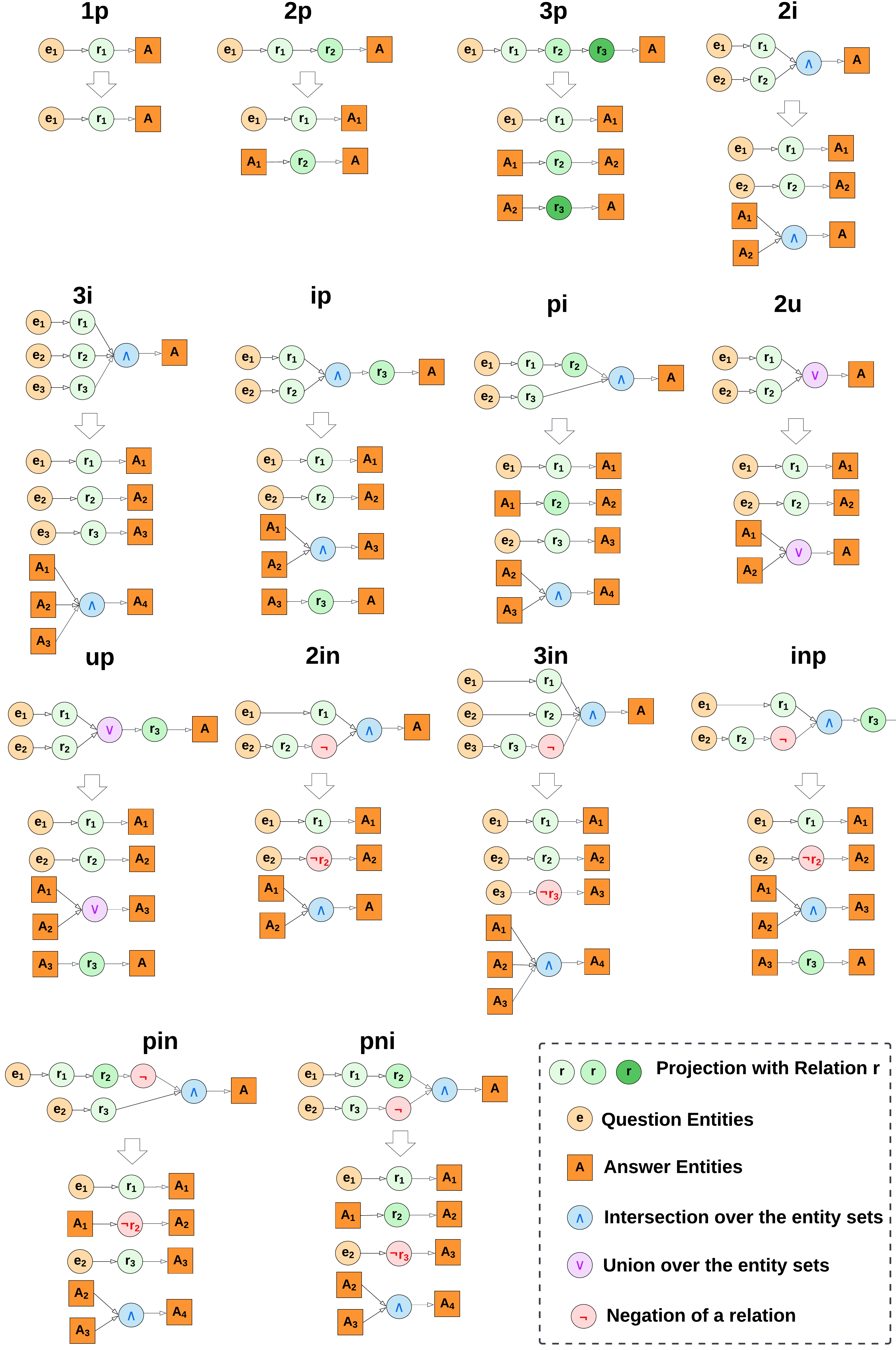## Appendix ## Appendix A Query Decomposition of Different Query Types Figure 4 provides the query decomposition of different query types considered in our empirical study as well as previous literature in the area. <details> <summary>extracted/2305.01157v3/images/query_decomposition.png Details</summary>  ### Visual Description ## Flowchart Diagram: Entity Relation Operations ### Overview The image depicts a multi-panel flowchart diagram illustrating logical operations on entity sets. It consists of 16 panels arranged in a 4x4 grid, each demonstrating different configurations of question entities (e), answer entities (A), and relational operations (Λ, ∨, ¬r). The diagram uses color-coded symbols to represent entities and operations, with arrows indicating directional flow. ### Components/Axes **Legend (bottom-right):** - **Circles**: Question Entities (e) - Light orange: e₁ - Light green: e₂ - Light blue: e₃ - **Rectangles**: Answer Entities (A) - Orange: A₁, A₂, A₃, A₄ - **Operations**: - Blue circle (Λ): Intersection over entity sets - Purple circle (∨): Union over entity sets - Red circle (¬r): Negation of a relation - Green circles (r): Projection with Relation r **Panel Structure**: - All panels follow a left-to-right flow - Entities (e/A) are positioned on the left/right - Operations (Λ/∨/¬r) are central connectors - Arrows show directional relationships ### Detailed Analysis **Panel Configurations**: 1. **1p**: e₁ → r₁ → A 2. **2p**: e₁ → r₁ → A₁; e₁ → r₂ → A 3. **3p**: e₁ → r₁ → A₁; A₁ → r₂ → A₂; A₂ → r₃ → A 4. **2i**: e₁ → r₁ → A₁; e₂ → r₂ → A₂; A₁ ∨ A₂ → A 5. **3i**: e₁ → r₁ → A; e₂ → r₂ → A; e₃ → r₃ → A; A₁ ∧ A₂ ∧ A₃ → A 6. **ip**: e₁ → r₁ → A; e₂ → r₂ → A; r₃ → A 7. **pi**: e₁ → r₁ → A; e₂ → r₃ → A; A₁ ∧ A₂ → A 8. **2u**: e₁ → r₁ → A₁; e₂ → r₂ → A₂; A₁ ∨ A₂ → A 9. **up**: e₁ → r₁ → A₁; e₂ → r₂ → A₂; e₃ → r₃ → A₃; A₁ ∧ A₂ ∧ A₃ → A 10. **2in**: e₁ → r₁ → A₁; e₂ → r₂ → A₂; A₁ ∨ A₂ → A₃ 11. **3in**: e₁ → r₁ → A; e₂ → r₂ → A; e₃ → ¬r₃ → A 12. **inp**: e₁ → r₁ → A₁; e₂ → ¬r₂ → A₂; A₁ ∧ A₂ → A 13. **pin**: e₁ → r₁ → A₁; e₂ → r₃ → A₃; A₁ ∧ A₂ → A 14. **pni**: e₁ → r₁ → A₁; e₂ → ¬r₃ → A₃; A₁ ∧ A₂ → A **Color Consistency Check**: - All green circles (r) match legend - Blue circles (Λ) consistently represent intersection - Purple circles (∨) consistently represent union - Red circles (¬r) consistently represent negation ### Key Observations 1. **Complexity Progression**: Panels increase in complexity from single-entity operations (1p) to multi-entity combinations (3i, up) 2. **Negation Patterns**: Panels with ¬r (3in, inp, pni) demonstrate logical negation operations </details> Figure 4: Query Decomposition of different query types considered in our experiments. ## Appendix B Prompt Templates of Different Query Types The prompt templates for full complex logical queries with multiple operations and decomposed elementary logical queries with single operation are provided in Tables 5 and 6, respectively. Table 5: Full Prompt Templates of Different Query Types. | Context | $\mathcal{N}_{k}(q_{\tau}[Q_{\tau}])$ | Given the following (h,r,t) triplets where entity h is related to entity t by relation r; $(h_{1},r_{1},t_{1}),(h_{2},r_{2},t_{2}),(h_{3},r_{3},t_{3}),(h_{4},r_{4},t_{4}),$ | | --- | --- | --- | | $(h_{5},r_{5},t_{5}),(h_{6},r_{6},t_{6}),(h_{7},r_{7},t_{7}),(h_{8},r_{8},t_{8})$ | | | | 1p | $\exists X.r_{1}(X,e_{1})$ | Which entities are connected to $e_{1}$ by relation $r_{1}$ ? | | 2p | $\exists X.r_{1}(X,\exists Y.r_{2}(Y,e_{1})$ | Let us assume that the set of entities E is connected to entity $e_{1}$ by relation $r_{1}$ . Then, what are the entities connected to E by relation $r_{2}$ ? | | 3p | $\exists X.r_{1}(X,\exists Y.r_{2}(Y,\exists Z.r_{3}(Z,e_{1})$ | Let us assume that the set of entities E is connected to entity $e_{1}$ by relation $r_{1}$ and the set of entities F is connected to entities in E by relation $r_{2}$ . Then, what are the entities connected to F by relation $r_{3}$ ? | | 2i | $\exists X.[r_{1}(X,e_{1})\wedge r_{2}(X,e_{2})]$ | Let us assume that the set of entities E is connected to entity $e_{1}$ by relation $r_{1}$ and the set of entities F is connected to entity $e_{2}$ by relation $r_{2}$ . Then, what are the entities in the intersection of set E and F, i.e., entities present in both F and G? | | 3i | $\exists X.[r_{1}(X,e_{1})\wedge r_{2}(X,e_{2})\wedge r_{3}(X,e_{3})]$ | Let us assume that the set of entities E is connected to entity $e_{1}$ by relation $r_{1}$ , the set of entities F is connected to entity $e_{2}$ by relation $r_{2}$ and the set of entities G is connected to entity $e_{3}$ by relation $r_{3}$ . Then, what are the entities in the intersection of set E, F and G, i.e., entities present in all E, F and G? | | ip | $\exists X.r_{3}(X,\exists Y.[r_{1}(Y,e_{1})\wedge r_{2}(Y,e_{2})]$ | Let us assume that the set of entities E is connected to entity $e_{1}$ by relation $r_{1}$ , F is the set of entities connected to entity $e_{2}$ by relation $r_{2}$ , and G is the set of entities in the intersection of E and F. Then, what are the entities connected to entities in set G by relation $r_{3}$ ? | | pi | $\exists X.[r_{1}(X,\exists Y.r_{2}(Y,e_{2}))\wedge r_{3}(X,e_{3})]$ | Let us assume that the set of entities E is connected to entity $e_{1}$ by relation $r_{1}$ , F is the set of entities connected to entities in E by relation $r_{2}$ , and G is the set of entities connected to entity $e_{2}$ by relation $r_{3}$ . Then, what are the entities in the intersection of set F and G, i.e., entities present in both F and G? | | 2u | $\exists X.[r_{1}(X,e_{1})\vee r_{2}(X,e_{2})]$ | Let us assume that the set of entities E is connected to entity $e_{1}$ by relation $r_{1}$ and F is the set of entities connected to entity $e_{2}$ by relation $r_{2}$ . Then, what are the entities in the union of set F and G, i.e., entities present in either F or G? | | up | $\exists X.r_{3}(X,\exists Y.[r_{1}(Y,e_{1})\vee r_{2}(Y,e_{2})]$ | Let us assume that the set of entities E is connected to entity $e_{1}$ by relation $r_{1}$ and F is the set of entities connected to entity $e_{2}$ by relation $r_{2}$ . G is the set of entities in the union of E and F. Then, what are the entities connected to entities in G by relation $r_{3}$ ? | | 2in | $\exists X.[r_{1}(X,e_{1})\wedge\neg r_{2}(X,e_{2})]$ | Let us assume that the set of entities E is connected to entity $e_{1}$ by relation $r_{1}$ and F is the set of entities connected to entity $e_{2}$ by any relation other than relation $r_{2}$ . Then, what are the entities in the intersection of set E and F, i.e., entities present in both F and G? | | 3in | $\exists X.[r_{1}(X,e_{1})\wedge r_{2}(X,e_{2})\wedge\neg r_{3}(X,e_{3})]$ | Let us assume that the set of entities E is connected to entity $e_{1}$ by relation $r_{1}$ , F is the set of entities connected to entity $e_{2}$ by relation $r_{2}$ , and F is the set of entities connected to entity $e_{3}$ by any relation other than relation $r_{3}$ . Then, what are the entities in the intersection of set E and F, i.e., entities present in both F and G? | | inp | $\exists X.r_{3}(X,\exists Y.[r_{1}(Y,e_{1})\wedge\neg r_{2}(Y,e_{2})]$ | Let us assume that the set of entities E is connected to entity $e_{1}$ by relation $r_{1}$ , and F is the set of entities connected to entity $e_{2}$ by any relation other than relation $r_{2}$ . Then, what are the entities that are connected to the entities in the intersection of set E and F by relation $r_{3}$ ? | | pin | $\exists X.[r_{1}(X,\exists Y.\neg r_{2}(Y,e_{2}))\wedge r_{3}(X,e_{3})]$ | Let us assume that the set of entities E is connected to entity $e_{1}$ by relation $r_{1}$ , F is the set of entities connected to entities in E by relation $r_{2}$ , and G is the set of entities connected to entity $e_{2}$ by any relation other than relation $r_{3}$ . Then, what are the entities in the intersection of set F and G, i.e., entities present in both F and G? | | pni | $\exists X.[r_{1}(X,\exists Y.\neg r_{2}(Y,e_{2}))\wedge\neg r_{3}(X,e_{3})]$ | Let us assume that the set of entities E is connected to entity $e_{1}$ by relation $r_{1}$ , F is the set of entities connected to entities in E by any relation other than $r_{2}$ , and G is the set of entities connected to entity $e_{2}$ by relation $r_{3}$ . Then, what are the entities in the intersection of set F and G, i.e., entities present in both F and G? | Table 6: Decomposed Prompt Templates of Different Query Types. | Context | $\mathcal{N}_{k}(q_{\tau}[Q_{\tau}])$ | Given the following (h,r,t) triplets where entity h is related to entity t by relation r; $(h_{1},r_{1},t_{1}),(h_{2},r_{2},t_{2}),(h_{3},r_{3},t_{3}),(h_{4},r_{4},t_{4}),$ | | --- | --- | --- | | $(h_{5},r_{5},t_{5}),(h_{6},r_{6},t_{6}),(h_{7},r_{7},t_{7}),(h_{8},r_{8},t_{8})$ | | | | 1p | $\exists X.r_{1}(X,e_{1})$ | Which entities are connected to $e_{1}$ by relation $r_{1}$ ? | | 2p | $\exists X.r_{1}(X,\exists Y.$ | Which entities are connected to $e_{1}$ by relation $r_{1}$ ? | | $r_{2}(Y,e_{1})$ | Which entities are connected to any entity in [PP1] by relation $r_{2}$ ? | | | 3p | $\exists X.r_{1}(X,\exists Y$ | Which entities are connected to $e_{1}$ by relation $r_{1}$ ? | | $.r_{2}(Y,\exists Z.$ | Which entities are connected to any entity in [PP1] by relation $r_{2}$ ? | | | $r_{3}(Z,e_{1})$ | Which entities are connected to any entity in [PP2] by relation $r_{3}$ ? | | | 2i | $\exists X.[r_{1}(X,e_{1})$ | Which entities are connected to $e_{1}$ by relation $r_{1}$ ? | | $\wedge r_{2}(X,e_{2})]$ | Which entities are connected to $e_{2}$ by relation $r_{2}$ ? | | | What are the entities in the intersection of entity sets [PP1] and [PP2]? | | | | 3i | $\exists X.[r_{1}(X,e_{1})$ | Which entities are connected to $e_{1}$ by relation $r_{1}$ ? | | $\wedge r_{2}(X,e_{2})$ | Which entities are connected to $e_{2}$ by relation $r_{2}$ ? | | | $\wedge r_{3}(X,e_{3})]$ | Which entities are connected to $e_{3}$ by relation $r_{3}$ ? | | | What are the entities in the intersection of entity sets [PP1], [PP2] and [PP3]? | | | | ip | $\exists X.r_{3}(X,\exists Y.[r_{1}(Y,e_{1})$ | Which entities are connected to $e_{1}$ by relation $r_{1}$ ? | | $\wedge r_{2}(Y,e_{2})]$ | Which entities are connected to $e_{2}$ by relation $r_{2}$ ? | | | What are the entities in the intersection of entity sets [PP1] and [PP2]? | | | | What are the entities connected to any entity in [PP3] by relation $r_{3}$ ? | | | | pi | $\exists X.[r_{1}(X,\exists Y.r_{2}(Y,e_{2}))$ | Which entities are connected to $e_{1}$ by relation $r_{1}$ ? | | $\wedge r_{3}(X,e_{3})]$ | Which entities are connected to [PP1] by relation $r_{2}$ ? | | | Which entities are connected to $e_{2}$ by relation $r_{3}$ ? | | | | What are the entities in the intersection of entity sets [PP2] and [PP3]? | | | | 2u | $\exists X.[r_{1}(X,e_{1})$ | Which entities are connected to $e_{1}$ by relation $r_{1}$ ? | | $\vee r_{2}(X,e_{2})]$ | Which entities are connected to $e_{2}$ by relation $r_{2}$ ? | | | What are the entities in the union of entity sets [PP1] and [PP2]? | | | | up | $\exists X.r_{3}(X,\exists Y.[r_{1}(Y,e_{1})$ | Which entities are connected to $e_{1}$ by relation $r_{1}$ ? | | $\vee r_{2}(Y,e_{2})]$ | Which entities are connected to $e_{2}$ by relation $r_{2}$ ? | | | What are the entities in the union of entity sets [PP1] and [PP2]? | | | | Which entities are connected to any entity in [PP3] by relation $r_{3}$ ? | | | | 2in | $\exists X.[r_{1}(X,e_{1})$ | Which entities are connected to $e_{1}$ by any relation other than $r_{1}$ ? | | $\wedge\neg r_{2}(X,e_{2})]$ | Which entities are connected to $e_{2}$ by any relation other than $r_{2}$ ? | | | What are the entities in the intersection of entity sets [PP1] and [PP2]? | | | | 3in | $\exists X.[r_{1}(X,e_{1})$ | Which entities are connected to $e_{1}$ by any relation other than $r_{1}$ ? | | $\wedge r_{2}(X,e_{2})$ | Which entities are connected to $e_{2}$ by any relation other than $r_{2}$ ? | | | $\wedge\neg r_{3}(X,e_{3})]$ | Which entities are connected to $e_{3}$ by any relation other than $r_{3}$ ? | | | What are the entities in the intersection of entity sets [PP1], [PP2] and [PP3]? | | | | inp | $\exists X.r_{3}(X,\exists Y.[r_{1}(Y,e_{1})$ | Which entities are connected to $e_{1}$ by relation $r_{1}$ ? | | $\wedge\neg r_{2}(Y,e_{2})]$ | Which entities are connected to $e_{2}$ by any relation other than $r_{2}$ ? | | | What are the entities in the intersection of entity sets [PP1], and [PP2]? | | | | What are the entities connected to any entity in [PP3] by relation $r_{3}$ ? | | | | pin | $\exists X.[r_{1}(X,\exists Y.\neg r_{2}(Y,e_{2}))$ | Which entities are connected to $e_{1}$ by relation $r_{1}$ ? | | $\wedge r_{3}(X,e_{3})]$ | Which entities are connected to entity set in [PP1] by relation $r_{2}$ ? | | | Which entities are connected to $e_{2}$ by any relation other than $r_{3}$ ? | | | | What are the entities in the intersection of entity sets [PP2] and [PP3]? | | | | pni | $\exists X.[r_{1}(X,\exists Y.\neg r_{2}(Y,e_{2}))$ | Which entities are connected to $e_{1}$ by relation $r_{1}$ ? | | $\wedge\neg r_{3}(X,e_{3})]$ | Which entities are connected to any entity in [PP1] by any relation other than $r_{2}$ ? | | | Which entities are connected to $e_{2}$ by relation $r_{3}$ ? | | | | What are the entities in the intersection of entity sets [PP2] and [PP3]? | | | ## Appendix C Analysis of Logical Reasoning Performance using HITS Metric Tables 7 and 8 present the HITS@K=3 results of baselines and our model. HITS@K indicates the accuracy of predicting correct candidates in the top-K results. Table 7: Performance comparison study between LARK and the baseline, focusing on their efficacy of logical reasoning using HITS@K=1,3,10 scores. The rows correspond to the models and columns denote the different query structures of multi-hop projections, geometric operations, and compound operations. The best results for each query type in every dataset are highlighted in bold font. | Dataset FB15k | Variant Llama2-7B | 1p HITS@1 74.6 | 2p 26 | 3p 18.5 | 2i 59.9 | 3i 47.7 | ip 2.4 | pi 5.7 | 2u 5.8 | up 5 | | --- | --- | --- | --- | --- | --- | --- | --- | --- | --- | --- | | complex | 77.5 | 37.9 | 26.3 | 67.4 | 54.6 | 8.2 | 20.7 | 20.7 | 17.6 | | | step | 77.5 | 41.8 | 28.1 | 70.2 | 57.3 | 10.3 | 24.3 | 22.8 | 17.8 | | | FB15k-237 | Llama2-7B | 77.2 | 28.5 | 17.7 | 10.9 | 22.6 | 10.8 | 8.7 | 10.5 | 13.2 | | complex | 78.5 | 30.8 | 19.3 | 41.1 | 38.1 | 9.6 | 18.7 | 24.2 | 14.0 | | | step | 78.5 | 34.3 | 21.3 | 43.2 | 40.2 | 11.7 | 22.2 | 27.9 | 14.2 | | | NELL995 | Llama2-7B | 86.4 | 28.3 | 19.6 | 10.2 | 24 | 8.6 | 3.5 | 1.5 | 15.9 | | complex | 88.0 | 30.9 | 21.7 | 44.1 | 41.6 | 7.4 | 8.2 | 3.3 | 17 | | | step | 88.0 | 34.3 | 24.0 | 46.1 | 43.8 | 9.5 | 9.8 | 8.9 | 17.3 | | | HITS@3 | | | | | | | | | | | | FB15k | Llama2-7B | 74 | 53.4 | 34.6 | 18.2 | 36.4 | 44.7 | 39.4 | 35.7 | 77.1 | | complex | 77.7 | 57.6 | 37.9 | 68.5 | 61.3 | 39.6 | 84.8 | 82.9 | 81.7 | | | step | 77.7 | 57.4 | 40.1 | 69.4 | 62.5 | 48.4 | 91.2 | 92.7 | 82.6 | | | FB15k-237 | Llama2-7B | 75.9 | 42.6 | 25.7 | 12.6 | 25.9 | 43.6 | 35.1 | 42.9 | 53.8 | | complex | 78.3 | 45.9 | 28.1 | 47.2 | 43.7 | 38.7 | 75.6 | 89.4 | 57 | | | step | 78.3 | 45.9 | 29.8 | 48.2 | 44.6 | 47.3 | 80.0 | 93.6 | 57.6 | | | NELL995 | Llama2-7B | 85.6 | 42.9 | 28.7 | 11.8 | 27.6 | 34.6 | 14.1 | 5.7 | 65 | | complex | 87.8 | 46.8 | 31.6 | 50.7 | 47.9 | 29.8 | 32.9 | 13.2 | 69.4 | | | step | 87.8 | 45.7 | 33.5 | 51.3 | 48.7 | 38.1 | 39.6 | 35.8 | 70.3 | | | HITS@10 | | | | | | | | | | | | FB15k | Llama2-7B | 73.6 | 53.9 | 35.7 | 18.1 | 36.3 | 44.6 | 39.5 | 35.7 | 77.1 | | complex | 77.7 | 58.2 | 39.1 | 68.2 | 61.4 | 39.5 | 85 | 82.9 | 81.7 | | | step | 77.7 | 57.4 | 46.0 | 69.4 | 62.5 | 48.2 | 91.2 | 84.7 | 82.6 | | | FB15k-237 | Llama2-7B | 75.2 | 43 | 26.5 | 12.6 | 25.9 | 43.6 | 35.1 | 42.9 | 53.8 | | complex | 78.3 | 46.4 | 29 | 47.3 | 43.8 | 38.7 | 75.6 | 89.4 | 57 | | | step | 78.3 | 45.9 | 34.1 | 48.2 | 44.6 | 47.3 | 80.0 | 93.6 | 57.6 | | | NELL995 | Llama2-7B | 84.9 | 43.4 | 29.2 | 11.8 | 27.6 | 34.6 | 14.1 | 5.7 | 65 | | complex | 87.8 | 47.4 | 32.2 | 50.8 | 48 | 29.8 | 32.9 | 13.2 | 69.4 | | | step | 87.8 | 45.7 | 38.3 | 51.3 | 48.7 | 38.1 | 39.6 | 35.8 | 70.3 | | Table 8: Performance comparison between LARK and the baseline for negation query types using HITS@K=1,3,10 scores. The best results for each query type in every dataset are given in bold font. | FB15k | Llama2-7B complex step | 1.8 6.7 7.4 | 0.7 2.4 2.7 | 4.0 14.2 14.9 | 2.1 7.8 9.1 | 0.9 3.3 3.4 | 18.6 26.6 31.0 | 5.7 9.5 12.1 | 40.8 59.2 64.8 | 18.8 30.3 38.7 | 8.6 12.3 14.4 | 18.6 26.6 31.0 | 5.7 9.5 12.1 | 40.8 59.3 64.8 | 18.8 30.3 38.7 | 8.6 12.4 14.4 | | --- | --- | --- | --- | --- | --- | --- | --- | --- | --- | --- | --- | --- | --- | --- | --- | --- | | FB15k-237 | Llama2-7B | 1.9 | 0.8 | 6.8 | 2.8 | 0.7 | 7.5 | 3.5 | 27.3 | 11.6 | 2.7 | 7.5 | 3.5 | 27.3 | 11.6 | 2.7 | | complex | 2.7 | 1.4 | 9.8 | 4.6 | 1 | 10.8 | 5.8 | 39.6 | 18.7 | 3.9 | 10.8 | 5.8 | 39.6 | 18.7 | 3.9 | | | step | 3.2 | 1.7 | 10.6 | 5.8 | 1.1 | 12.6 | 7.4 | 43.3 | 23.9 | 4.6 | 12.6 | 7.4 | 43.3 | 23.9 | 4.6 | | | NELL995 | Llama2-7B | 2.8 | 1.4 | 7.2 | 2.2 | 1.5 | 11.2 | 6 | 29.1 | 9.2 | 6.2 | 11.2 | 6 | 29.1 | 9.2 | 6.2 | | complex | 3.9 | 2.3 | 10.2 | 3.7 | 2.2 | 16.1 | 9.4 | 41.8 | 15.1 | 9 | 16.1 | 9.4 | 41.8 | 15.1 | 9 | | | step | 4.6 | 2.8 | 11.1 | 4.7 | 2.7 | 18.5 | 12.0 | 46.0 | 19.3 | 10.9 | 18.5 | 12.0 | 46.0 | 19.3 | 10.9 | | ## Appendix D Algorithm Algorithm for the LARK’s procedure is provided in Algorithm 1. Input: Logical query $q_{\tau}$ , Knowledge Graph $\mathcal{G}:E\times R$ ; Output: Answer entities $V_{\tau}$ ; 1 # Query Abstraction: Map entity and relations to IDs 2 $q_{\tau}=Abstract(q_{\tau});$ 3 $\mathcal{G}=Abstract(\mathcal{G});$ 4 # Neighborhood Retrieval 5 $\mathcal{N}_{k}(q_{\tau}[Q_{\tau}])=\left\{(h,r,t)\right\}$ , using Eq. (7) 6 # Query Decomposition 7 $q^{d}_{\tau}=Decomp(q_{\tau});$ 8 # Initialize Answer Cache $ans=\{\}$ ; 9 for $i\in 1:length\left(q^{d}_{\tau}\right)$ do 10 # Replace Answer Cache in Question 11 $q^{d}_{\tau}[i]=replace(q^{d}_{\tau}[i],ans[i-1]);$ 12 $ans[i]=LLM\left(q^{d}_{\tau}[i]\right);$ 13 14 end for return $ans[length\left(q^{d}_{\tau}\right)]$ Algorithm 1 LARK Algorithm Table 9: Details of the token distribution for various query types in different datasets. The columns present the mean, median, minimum (Min), and maximum (Max) values of the number of tokens in the queries of different query types. Column ‘Cov’ presents the percentage of queries (coverage) that contain less than 4096 tokens, which is the token limit of Llama2 model. | 1p | 70.2 | 61 | 58 | 10338 | 100 | 82.1 | 61 | 58 | 30326 | 99.9 | 81.7 | 61 | 58 | 30250 | 99.9 | | --- | --- | --- | --- | --- | --- | --- | --- | --- | --- | --- | --- | --- | --- | --- | --- | | 2p | 331.2 | 106 | 86 | 27549 | 97.1 | 1420.9 | 140 | 83 | 130044 | 89.7 | 893.4 | 136 | 83 | 108950 | 90.9 | | 3p | 785.2 | 165 | 103 | 80665 | 91 | 3579.8 | 329 | 103 | 208616 | 75.7 | 3052.6 | 389 | 100 | 164545 | 73.7 | | 2i | 1136.7 | 276 | 119 | 20039 | 86.3 | 4482.8 | 636 | 119 | 60655 | 67.7 | 4469.3 | 680 | 119 | 54916 | 67.3 | | 3i | 2575.4 | 860 | 145 | 29148 | 68.4 | 8760.2 | 2294 | 145 | 85326 | 48.3 | 8979.4 | 2856 | 145 | 76834 | 44.8 | | ip | 1923.8 | 1235 | 135 | 21048 | 67.4 | 4035.8 | 2017 | 131 | 32795 | 50.5 | 4838 | 2676 | 131 | 33271 | 43.6 | | pi | 1036.8 | 455 | 140 | 10937 | 85.8 | 1255.6 | 343 | 141 | 45769 | 83.4 | 1535.3 | 435 | 135 | 21125 | 79.9 | | 2u | 1325.4 | 790 | 121 | 14703 | 80.8 | 2109.5 | 868 | 123 | 60655 | 68.9 | 2294.9 | 1138 | 125 | 23637 | 65.7 | | up | 115.3 | 112 | 110 | 958 | 100 | 113.7 | 112 | 110 | 981 | 100 | 113.2 | 112 | 110 | 427 | 100 | | 2in | 1169.1 | 548 | 123 | 18016 | 84.9 | 5264.7 | 1116 | 128 | 60281 | 61.8 | 3496 | 774 | 124 | 58032 | 71.6 | | 3in | 4070.3 | 2230 | 159 | 28679 | 46.6 | 13695.8 | 8344 | 175 | 88561 | 25.9 | 12575.9 | 7061 | 164 | 88250 | 28.1 | | inp | 629 | 112 | 110 | 73457 | 91.8 | 1949.4 | 394 | 110 | 115169 | 78.4 | 696.7 | 112 | 110 | 89660 | 93.8 | | pin | 400.7 | 154 | 129 | 6802 | 95.8 | 1106.5 | 242 | 129 | 44010 | 87.2 | 418.1 | 131 | 129 | 24062 | 96.7 | | pni | 345.9 | 129 | 127 | 7938 | 96.6 | 547.1 | 129 | 127 | 18057 | 95.1 | 289.3 | 129 | 127 | 17489 | 97.9 | ## Appendix E Query Token Distribution in Datasets The quantitative details of the query token’s lengths is provided in Table 9 and their complete distribution plots are provided in Figure 5. From the results, we observe that the distribution of token lengths is positively-skewed for most of the query types, which indicates that the number of samples with high token lengths is small in number. Thus, small improvements in the LLMs’ token limit can potentially lead to better coverage on most of the reasoning queries in standard KG datasets. 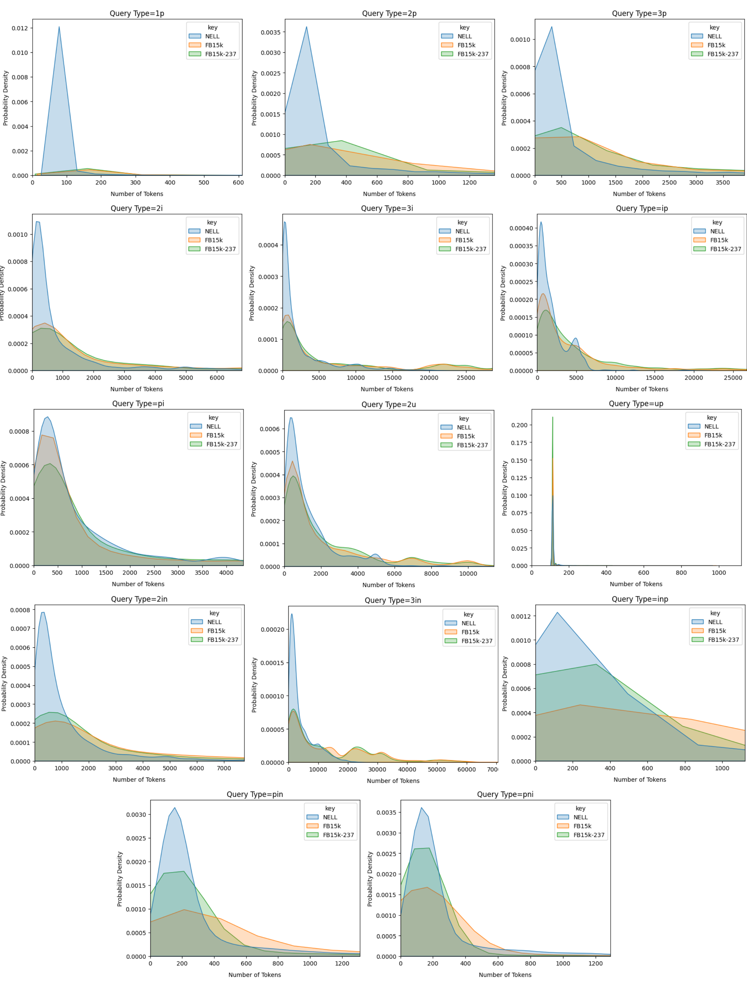<details> <summary>extracted/2305.01157v3/images/prob_dist.png Details</summary>  ### Visual Description ## Line Graphs: Probability Density Distributions Across Query Types and Models ### Overview The image displays 14 line graphs arranged in a grid, each representing the probability density distribution of token counts for different query types (e.g., `1p`, `2p`, `3p`, `ip`, `pi`, `up`, `in`, `inp`, `pin`, `2i`, `3i`, `2u`, `3u`). Three models are compared: `key` (blue), `NELL` (orange), and `FB15k-237` (green). Each graph shows how token counts are probabilistically distributed for a specific query type across these models. --- ### Components/Axes - **X-Axis**: "Number of Tokens" (ranges vary per graph, e.g., 0–600 for `1p`, 0–1200 for `2p`, up to 10,000 for `2u`). - **Y-Axis**: "Probability Density" (consistent scale: 0.0000 to 0.0012). - **Legend**: Located in the top-right corner of each graph, with labels: - `key` (blue) - `NELL` (orange) - `FB15k-237` (green) - **Graph Titles**: Positioned at the top of each subplot, labeled with query types (e.g., `Query Type=1p`, `Query Type=2p`). --- ### Detailed Analysis #### Query Type `1p` - **Key (blue)**: Sharp peak at ~100 tokens (probability density ~0.0012). - **NELL (orange)**: Broader distribution, peaking at ~150 tokens (density ~0.0008). - **FB15k-237 (green)**: Flattest distribution, peaking at ~200 tokens (density ~0.0005). #### Query Type `2p` - **Key (blue)**: Peak at ~200 tokens (density ~0.0035). - **NELL (orange)**: Broader peak at ~300 tokens (density ~0.0025). - **FB15k-237 (green)**: Gradual decline from ~400 tokens (density ~0.0015). #### Query Type `3p` - **Key (blue)**: Peak at ~500 tokens (density ~0.0010). - **NELL (orange)**: Broader peak at ~700 tokens (density ~0.0008). - **FB15k-237 (green)**: Flattest distribution, peaking at ~1,000 tokens (density ~0.0005). #### Query Type `ip` - **Key (blue)**: Sharp peak at ~200 tokens (density ~0.0004). - **NELL (orange)**: Broader peak at ~300 tokens (density ~0.0002). - **FB15k-237 (green)**: Flattest distribution, peaking at ~500 tokens (density ~0.0001). #### Query Type `pi` - **Key (blue)**: Sharp peak at ~1,000 tokens (density ~0.0008). - **NELL (orange)**: Broader peak at ~1,500 tokens (density ~0.0005). - **FB15k-237 (green)**: Flattest distribution, peaking at ~2,000 tokens (density ~0.0003). #### Query Type `up` - **Key (blue)**: Single sharp peak at ~200 tokens (density ~0.20). - **NELL (orange)**: Minimal presence, negligible density. - **FB15k-237 (green)**: Minimal presence, negligible density. #### Query Type `in` - **Key (blue)**: Sharp peak at ~1,000 tokens (density ~0.0020). - **NELL (orange)**: Broader peak at ~2,000 tokens (density ~0.0010). - **FB15k-237 (green)**: Flattest distribution, peaking at ~3,000 tokens (density ~0.0005). #### Query Type `inp` - **Key (blue)**: Sharp peak at ~500 tokens (density ~0.0012). - **NELL (orange)**: Broader peak at ~800 tokens (density ~0.0008). - **FB15k-237 (green)**: Flattest distribution, peaking at ~1,200 tokens (density ~0.0005). #### Query Type `pin` - **Key (blue)**: Sharp peak at ~300 tokens (density ~0.0030). - **NELL (orange)**: Broader peak at ~500 tokens (density ~0.0020). - **FB15k-237 (green)**: Flattest distribution, peaking at ~700 tokens (density ~0.0010). #### Query Type `pi` (Repeated) - Same as earlier `pi` analysis. #### Query Type `2i` - **Key (blue)**: Sharp peak at ~1,000 tokens (density ~0.0008). - **NELL (orange)**: Broader peak at ~2,000 tokens (density ~0.0005). - **FB15k-237 (green)**: Flattest distribution, peaking at ~3,000 tokens (density ~0.0003). #### Query Type `3i` - **Key (blue)**: Sharp peak at ~5,000 tokens (density ~0.0004). - **NELL (orange)**: Broader peak at ~7,000 tokens (density ~0.0003). - **FB15k-237 (green)**: Flattest distribution, peaking at ~9,000 tokens (density ~0.0002). #### Query Type `2u` - **Key (blue)**: Sharp peak at ~5,000 tokens (density ~0.0006). - **NELL (orange)**: Broader peak at ~7,000 tokens (density ~0.0004). - **FB15k-237 (green)**: Flattest distribution, peaking at ~9,000 tokens (density ~0.0002). #### Query Type `3u` - **Key (blue)**: Sharp peak at ~10,000 tokens (density ~0.0003). - **NELL (orange)**: Broader peak at ~12,000 tokens (density ~0.0002). - **FB15k-237 (green)**: Flattest distribution, peaking at ~14,000 tokens (density ~0.0001). --- ### Key Observations 1. **Model Differences**: - `key` consistently shows sharp, narrow peaks, indicating precise token usage. - `NELL` exhibits broader distributions, suggesting variability in token requirements. - `FB15k-237` has the flattest distributions, implying uniform token usage across ranges. 2. **Query Type Trends**: - Complex query types (e.g., `3p`, `2u`, `3u`) require higher token counts. - Simpler query types (e.g., `1p`, `up`) cluster around lower token counts. 3. **Anomalies**: - The `up` query type (`Query Type=up`) has an extreme outlier: `key` dominates with a single sharp peak, while `NELL` and `FB15k-237` are negligible. --- ### Interpretation The data suggests that: - The `key` model is optimized for specific token counts, likely due to its precision in handling structured queries. - `NELL` and `FB15k-237` models exhibit trade-offs between flexibility and uniformity, with `NELL` being more variable and `FB15k-237` more consistent. - Query types with higher token counts (e.g., `3p`, `2u`) may involve more complex or ambiguous tasks, requiring models to explore wider token ranges. - The `up` query type’s dominance by `key` highlights its unique suitability for this specific task, possibly due to its simplicity or structured nature. This analysis underscores the importance of model selection based on query complexity and token efficiency requirements. </details> Figure 5: Probability distribution of the number of tokens in each query type. The figures contains 14 graphs for the 14 different query types. The x-axis and y-axis presents the number of tokens in the query and their probability density, respectively.