# On the Security Risks of Knowledge Graph Reasoning
**Authors**:
- Zhaohan Xi
- Penn State
- Tianyu Du
- Penn State
- Changjiang Li
- Penn State
- Ren Pang
- Penn State
- Shouling Ji (Zhejiang University)
- Xiapu Luo (Hong Kong Polytechnic University)
- Xusheng Xiao (Arizona State University)
- Fenglong Ma
- Penn State
- Ting Wang
- Penn State
mtbox[1]left=0.25mm, right=0.25mm, top=0.25mm, bottom=0.25mm, sharp corners, colframe=red!50!black, boxrule=0.5pt, title=#1, fonttitle=, coltitle=red!50!black, attach title to upper= –
## Abstract
Knowledge graph reasoning (KGR) – answering complex logical queries over large knowledge graphs – represents an important artificial intelligence task, entailing a range of applications (e.g., cyber threat hunting). However, despite its surging popularity, the potential security risks of KGR are largely unexplored, which is concerning, given the increasing use of such capability in security-critical domains.
This work represents a solid initial step towards bridging the striking gap. We systematize the security threats to KGR according to the adversary’s objectives, knowledge, and attack vectors. Further, we present ROAR, a new class of attacks that instantiate a variety of such threats. Through empirical evaluation in representative use cases (e.g., medical decision support, cyber threat hunting, and commonsense reasoning), we demonstrate that ROAR is highly effective to mislead KGR to suggest pre-defined answers for target queries, yet with negligible impact on non-target ones. Finally, we explore potential countermeasures against ROAR, including filtering of potentially poisoning knowledge and training with adversarially augmented queries, which leads to several promising research directions.
## 1 Introduction
Knowledge graphs (KGs) are structured representations of human knowledge, capturing real-world objects, relations, and their properties. Thanks to automated KG building tools [61], recent years have witnessed a significant growth of KGs in various domains (e.g., MITRE [10], GNBR [53], and DrugBank [4]). One major use of such KGs is knowledge graph reasoning (KGR), which answers complex logical queries over KGs, entailing a range of applications [6] such as information retrieval [8], cyber-threat hunting [2], biomedical research [30], and clinical decision support [12]. For instance, KG-assisted threat hunting has been used in both research prototypes [50, 34] and industrial platforms [9, 40].
**Example 1**
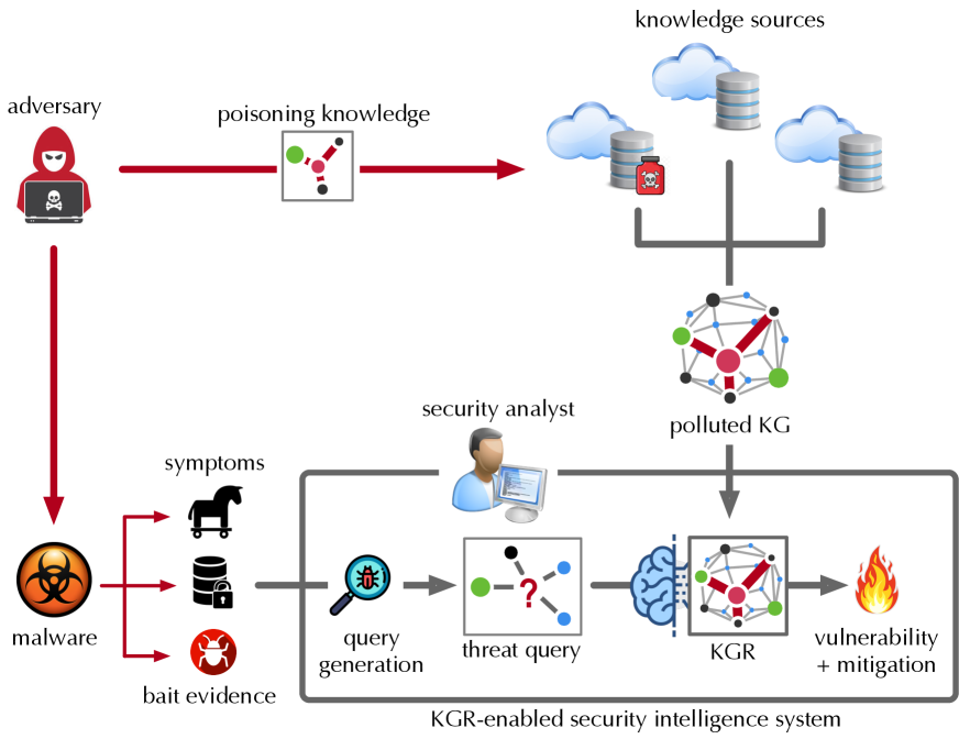
*In cyber threat hunting as shown in Figure 1, upon observing suspicious malware activities, the security analyst may query a KGR-enabled security intelligence system (e.g., LogRhythm [47]): “ how to mitigate the malware that targets BusyBox and launches DDoS attacks? ” Processing the query over the backend KG may identify the most likely malware as Mirai and its mitigation as credential-reset [15].*
<details>
<summary>x1.png Details</summary>
### Visual Description
## Diagram: KGR-Enabled Security Intelligence System Threat Model
### Overview
This diagram illustrates a cyber-security threat model involving an adversary who executes a two-pronged attack: data poisoning of knowledge sources and the deployment of malware. The diagram depicts how these actions flow into a "KGR-enabled security intelligence system," where a security analyst attempts to identify vulnerabilities and mitigations using Knowledge Graph Reasoning (KGR), potentially compromised by the adversary's actions.
### Components/Axes
The diagram is organized into a workflow with distinct functional areas:
* **Adversary (Top-Left):** Represented by a hooded figure with a laptop.
* **Knowledge Poisoning Path (Top):**
* **Poisoning Knowledge:** A graph icon with a red node.
* **Knowledge Sources:** Three cloud icons, each containing a database cylinder. One database is marked with a red poison/skull icon.
* **Polluted KG:** A complex network graph icon with thick red lines and nodes.
* **Malware/Symptoms Path (Bottom-Left):**
* **Malware:** A biohazard symbol.
* **Symptoms:** Three icons representing a Trojan horse, a locked database, and a bug.
* **Bait Evidence:** Label associated with the bug icon.
* **KGR-Enabled Security Intelligence System (Bottom-Center/Right):** A large, grey-outlined box containing:
* **Security Analyst:** An icon of a person at a computer.
* **Query Generation:** A magnifying glass icon inspecting a bug.
* **Threat Query:** A graph icon with a question mark.
* **KGR:** A brain icon connected to a network graph.
* **Vulnerability + Mitigation:** A fire icon.
### Detailed Analysis
**1. The Poisoning Workflow (Top Section):**
* The **Adversary** initiates a "poisoning knowledge" action (indicated by a thick red arrow).
* This action targets the **Knowledge Sources** (the clouds).
* The result is a **Polluted KG** (Knowledge Graph). The visual representation of the KG shows thick red lines, suggesting that the poisoned data has propagated through the network structure.
**2. The Malware/Detection Workflow (Bottom-Left Section):**
* The **Adversary** deploys **Malware** (biohazard icon).
* This malware manifests as **Symptoms** (Trojan horse, locked database, bug).
* The "bug" icon is specifically labeled as **Bait evidence**.
**3. The System Processing (Inside the KGR-Enabled System Box):**
* The **Security Analyst** oversees the process.
* The flow moves from the **Symptoms/Bait evidence** into **Query generation** (magnifying glass).
* This generates a **Threat query** (graph with a question mark).
* The query is processed by the **KGR** (Knowledge Graph Reasoning) engine, which is depicted as a brain icon connected to a network graph.
* The final output of the system is **Vulnerability + mitigation** (fire icon).
### Key Observations
* **Data Flow:** There are two distinct entry points for the adversary: one targeting the *knowledge base* (poisoning) and one targeting the *system environment* (malware).
* **Visual Metaphors:**
* The "poisoning" is represented by a red skull icon on a database and red lines in the graph, signifying corruption.
* The "KGR" is represented by a brain, implying an AI or machine-learning-based reasoning component.
* **System Integration:** The "Security Analyst" is positioned as a central figure, interacting with the query generation and the KGR engine, suggesting human-in-the-loop oversight.
### Interpretation
This diagram demonstrates a sophisticated attack vector known as **Knowledge Poisoning** against an AI-driven security system.
* **The Core Threat:** The adversary is not just attacking the target system directly with malware; they are attacking the *intelligence* of the system. By poisoning the "knowledge sources," the adversary ensures that the "Polluted KG" contains false or misleading information.
* **The Consequence:** When the "KGR" (Knowledge Graph Reasoning) engine processes a "threat query" based on the "polluted KG," the resulting "vulnerability + mitigation" output may be flawed. The system might fail to identify the actual malware, or it might suggest incorrect mitigations, effectively blinding the security analyst or leading them to take ineffective actions.
* **Peircean Investigative View:** The diagram suggests a "Trojan Horse" style of data manipulation. The "bait evidence" implies the adversary is intentionally leaving traces to trigger the system's detection mechanisms, ensuring the system processes the poisoned data. The system is designed to be "KGR-enabled," but the diagram serves as a warning that if the underlying knowledge graph is compromised, the reasoning engine's output becomes untrustworthy.
</details>
Figure 1: Threats to KGR-enabled security intelligence systems.
Surprisingly, in contrast to the growing popularity of using KGR to support decision-making in a variety of critical domains (e.g., cyber-security [52], biomedicine [12], and healthcare [71]), its security implications are largely unexplored. More specifically,
RQ ${}_{1}$ – What are the potential threats to KGR?
RQ ${}_{2}$ – How effective are the attacks in practice?
RQ ${}_{3}$ – What are the potential countermeasures?
Yet, compared with other machine learning systems (e.g., graph learning), KGR represents a unique class of intelligence systems. Despite the plethora of studies under the settings of general graphs [72, 66, 73, 21, 68] and predictive tasks [70, 54, 19, 56, 18], understanding the security risks of KGR entails unique, non-trivial challenges: (i) compared with general graphs, KGs contain richer relational information essential for KGR; (ii) KGR requires much more complex processing than predictive tasks (details in § 2); (iii) KGR systems are often subject to constant update to incorporate new knowledge; and (iv) unlike predictive tasks, the adversary is able to manipulate KGR through multiple different attack vectors (details in § 3).
<details>
<summary>x2.png Details</summary>
### Visual Description
## [Diagram Type]: Knowledge Graph Reasoning Process
### Overview
This image illustrates a three-part conceptual framework for performing reasoning over a knowledge graph. It moves from a static knowledge graph representation (a) to a formal query definition (b), and finally to a computational reasoning process (c) that resolves the query. The context is cybersecurity, specifically identifying mitigation strategies for malware targeting "BusyBox" devices.
### Components/Axes
The diagram uses a consistent color-coding scheme for nodes across all three sections:
* **Red Nodes:** Represent attack types (DDoS, PDoS).
* **Yellow Node:** Represents the target device (BusyBox).
* **Blue Nodes:** Represent specific malware instances (Mirai, Brickerbot).
* **Green Nodes:** Represent mitigation strategies (credential reset, hardware restore).
* **Grey Nodes:** Represent abstract variables or intermediate reasoning states.
### Detailed Analysis
#### (a) Knowledge Graph
This section displays the raw data structure.
* **Top Cluster:** A "DDoS" (red) node connects to "Mirai" (blue) via a "launch-by" edge. "BusyBox" (yellow) connects to "Mirai" (blue) via a "target-by" edge. "Mirai" (blue) connects to "credential reset" (green) via a "mitigate-by" edge.
* **Bottom Cluster:** "BusyBox" (yellow) connects to "Brickerbot" (blue) via a "target-by" edge. "PDoS" (red) connects to "Brickerbot" (blue) via a "launch-by" edge. "Brickerbot" (blue) connects to "hardware restore" (green) via a "mitigate-by" edge.
#### (b) Query
This section formalizes the natural language question into a graph-based query.
* **Text:** "How to mitigate the malware that targets BusyBox and launches DDoS attacks?"
* **Formalization:**
* $\mathcal{A}_q = \{\text{BusyBox, DDoS}\}$ (The set of known entities).
* $\mathcal{V}_q = \{v_{\text{malware}}\}$ (The variable to be solved).
* $\mathcal{E}_q = \{ \text{BusyBox} \xrightarrow{\text{target-by}} v_{\text{malware}}, \text{DDoS} \xrightarrow{\text{launch-by}} v_{\text{malware}}, v_{\text{malware}} \xrightarrow{\text{mitigate-by}} v_? \}$
* **Visual Graph:** Shows the query structure: A central variable node $v_{\text{malware}}$ (blue) is targeted by "BusyBox" (yellow) and launched by "DDoS" (red). The result $v_?$ (green) is the mitigation strategy.
#### (c) Knowledge Graph Reasoning
This section illustrates the computational flow, divided into four stages:
* **Stage (1):** Input embeddings $\phi_{\text{DDoS}}$ (red) and $\phi_{\text{BusyBox}}$ (yellow).
* **Stage (2):** Projection of inputs through relations $\psi_{\text{launch-by}}$ and $\psi_{\text{target-by}}$ into intermediate grey nodes.
* **Stage (3):** Intersection/Conjunction ($\psi_{\wedge}$) of the two paths into a single $v_{\text{malware}}$ node, followed by the application of the $\psi_{\text{mitigate-by}}$ relation to reach a final grey node.
* **Stage (4):** The final result $v_?$ is mapped to the green node $[q]$, representing the answer to the query.
### Key Observations
* **Logic Flow:** The diagram demonstrates a transition from symbolic data (a) to a formal query (b) to a vector-space or neural-symbolic reasoning process (c).
* **Conjunction:** The reasoning process in (c) explicitly uses a conjunction operator ($\psi_{\wedge}$) to combine the constraints of "launch-by" and "target-by," effectively filtering the knowledge graph to find the specific malware that satisfies both conditions.
* **Variable Resolution:** The notation $v_?$ represents the unknown entity (the mitigation strategy) that the system is attempting to retrieve.
### Interpretation
This diagram illustrates the architecture of a **Knowledge Graph Question Answering (KGQA)** system.
1. **Semantic Search:** The process demonstrates how a natural language question is decomposed into a subgraph pattern. The system does not just look for keywords; it looks for a specific path structure: `(DDoS) -> (launch-by) -> (Malware) <- (target-by) <- (BusyBox)`.
2. **Reasoning Mechanism:** The "Knowledge graph reasoning" section (c) suggests a neural-symbolic approach where entities and relations are embedded into a vector space ($\phi$ and $\psi$). The reasoning is performed by traversing these embeddings (projection) and intersecting them (conjunction) to isolate the correct answer.
3. **Utility:** This approach is highly effective for complex cybersecurity queries where the answer is not a single attribute but a relationship path. By identifying that "Mirai" is the only malware satisfying both the "DDoS" launch and "BusyBox" target criteria, the system can then traverse the "mitigate-by" edge to provide the correct remediation ("credential reset").
</details>
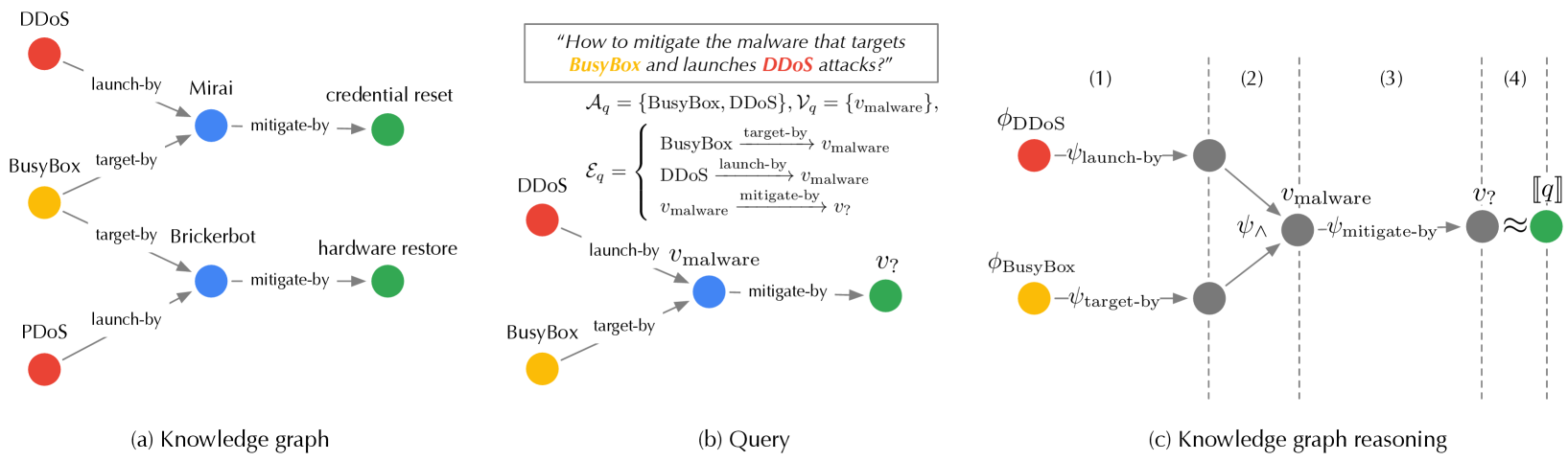
Figure 2: (a) sample knowledge graph; (b) sample query and its graph form; (c) reasoning over knowledge graph.
Our work. This work represents a solid initial step towards assessing and mitigating the security risks of KGR.
RA ${}_{1}$ – First, we systematize the potential threats to KGR. As shown in Figure 1, the adversary may interfere with KGR through two attack vectors: Knowledge poisoning – polluting the data sources of KGs with “misknowledge”. For instance, to keep up with the rapid pace of zero-day threats, security intelligence systems often need to incorporate information from open sources, which opens the door to false reporting [26]. Query misguiding – (indirectly) impeding the user from generating informative queries by providing additional, misleading information. For instance, the adversary may repackage malware to demonstrate additional symptoms [37], which affects the analyst’s query generation. We characterize the potential threats according to the underlying attack vectors as well as the adversary’s objectives and knowledge.
RA ${}_{2}$ – Further, we present ROAR, ROAR: R easoning O ver A dversarial R epresentations. a new class of attacks that instantiate the aforementioned threats. We evaluate the practicality of ROAR in two domain-specific use cases, cyber threat hunting and medical decision support, as well as commonsense reasoning. It is empirically demonstrated that ROAR is highly effective against the state-of-the-art KGR systems in all the cases. For instance, ROAR attains over 0.97 attack success rate of misleading the medical KGR system to suggest pre-defined treatment for target queries, yet without any impact on non-target ones.
RA ${}_{3}$ - Finally, we discuss potential countermeasures and their technical challenges. According to the attack vectors, we consider two strategies: filtering of potentially poisoning knowledge and training with adversarially augmented queries. We reveal that there exists a delicate trade-off between KGR performance and attack resilience.
Contributions. To our best knowledge, this work represents the first systematic study on the security risks of KGR. Our contributions are summarized as follows.
– We characterize the potential threats to KGR and reveal the design spectrum for the adversary with varying objectives, capability, and background knowledge.
– We present ROAR, a new class of attacks that instantiate various threats, which highlights the following features: (i) it leverages both knowledge poisoning and query misguiding as the attack vectors; (ii) it assumes limited knowledge regarding the target KGR system; (iii) it realizes both targeted and untargeted attacks; and (iv) it retains effectiveness under various practical constraints.
– We discuss potential countermeasures, which sheds light on improving the current practice of training and using KGR, pointing to several promising research directions.
## 2 Preliminaries
We first introduce fundamental concepts and assumptions.
Knowledge graphs (KGs). A KG ${\mathcal{G}}=({\mathcal{N}},{\mathcal{E}})$ consists of a set of nodes ${\mathcal{N}}$ and edges ${\mathcal{E}}$ . Each node $v\in{\mathcal{N}}$ represents an entity and each edge $v\mathrel{\text{\scriptsize$\xrightarrow[]{r}$}}v^{\prime}\in{\mathcal{E}}$ indicates that there exists relation $r\in{\mathcal{R}}$ (where ${\mathcal{R}}$ is a finite set of relation types) from $v$ to $v^{\prime}$ . In other words, ${\mathcal{G}}$ comprises a set of facts $\{\langle v,r,v^{\prime}\rangle\}$ with $v,v^{\prime}\in{\mathcal{N}}$ and $v\mathrel{\text{\scriptsize$\xrightarrow[]{r}$}}v^{\prime}\in{\mathcal{E}}$ .
**Example 2**
*In Figure 2 (a), the fact $\langle$ DDoS, launch-by, Mirai $\rangle$ indicates that the Mirai malware launches the DDoS attack.*
Queries. A variety of reasoning tasks can be performed over KGs [58, 33, 63]. In this paper, we focus on first-order conjunctive queries, which ask for entities that satisfy constraints defined by first-order existential ( $\exists$ ) and conjunctive ( $\wedge$ ) logic [59, 16, 60]. Formally, let ${\mathcal{A}}_{q}$ be a set of known entities (anchors), ${\mathcal{E}}_{q}$ be a set of known relations, ${\mathcal{V}}_{q}$ be a set of intermediate, unknown entities (variables), and $v_{?}$ be the entity of interest. A first-order conjunctive query $q\triangleq(v_{?},{\mathcal{A}}_{q},{\mathcal{V}}_{q},{\mathcal{E}}_{q})$ is defined as:
$$
\begin{split}&\llbracket q\rrbracket=v_{?}\,.\,\exists{\mathcal{V}}_{q}:\wedge
_{v\mathrel{\text{\scriptsize$\xrightarrow[]{r}$}}v^{\prime}\in{\mathcal{E}}_{
q}}v\mathrel{\text{\scriptsize$\xrightarrow[]{r}$}}v^{\prime}\\
&\text{s.t.}\;\,v\mathrel{\text{\scriptsize$\xrightarrow[]{r}$}}v^{\prime}=
\left\{\begin{array}[]{l}v\in{\mathcal{A}}_{q},v^{\prime}\in{\mathcal{V}}_{q}
\cup\{v_{?}\},r\in{\mathcal{R}}\\
v,v^{\prime}\in{\mathcal{V}}_{q}\cup\{v_{?}\},r\in{\mathcal{R}}\end{array}
\right.\end{split} \tag{1}
$$
Here, $\llbracket q\rrbracket$ denotes the query answer; the constraints specify that there exist variables ${\mathcal{V}}_{q}$ and entity of interest $v_{?}$ in the KG such that the relations between ${\mathcal{A}}_{q}$ , ${\mathcal{V}}_{q}$ , and $v_{?}$ satisfy the relations specified in ${\mathcal{E}}_{q}$ .
**Example 3**
*In Figure 2 (b), the query of “ how to mitigate the malware that targets BusyBox and launches DDoS attacks? ” can be translated into:
$$
\begin{split}q=&(v_{?},{\mathcal{A}}_{q}=\{\textsf{ BusyBox},\textsf{
DDoS}\},{\mathcal{V}}_{q}=\{v_{\text{malware}}\},\\
&{\mathcal{E}}_{q}=\{\textsf{ BusyBox}\scriptsize\mathrel{\stackunder[0
pt]{\xrightarrow{\makebox[24.86362pt]{$\scriptstyle\text{target-by}$}}}{
\scriptstyle\,}}v_{\text{malware}},\\
&\textsf{ DDoS}\scriptsize\mathrel{\stackunder[0pt]{\xrightarrow{
\makebox[26.07503pt]{$\scriptstyle\text{launch-by}$}}}{\scriptstyle\,}}v_{
\text{malware}},v_{\text{malware}}\scriptsize\mathrel{\stackunder[0pt]{
\xrightarrow{\makebox[29.75002pt]{$\scriptstyle\text{mitigate-by}$}}}{
\scriptstyle\,}}v_{?}\})\end{split} \tag{2}
$$*
Knowledge graph reasoning (KGR). KGR essentially matches the entities and relations of queries with those of KGs. Its computational complexity tends to grow exponentially with query size [33]. Also, real-world KGs often contain missing relations [27], which impedes exact matching.
Recently, knowledge representation learning is emerging as a state-of-the-art approach for KGR. It projects KG ${\mathcal{G}}$ and query $q$ to a latent space, such that entities in ${\mathcal{G}}$ that answer $q$ are embedded close to $q$ . Answering an arbitrary query $q$ is thus reduced to finding entities with embeddings most similar to $q$ , thereby implicitly imputing missing relations [27] and scaling up to large KGs [14]. Typically, knowledge representation-based KGR comprises two key components:
Embedding function $\phi$ – It projects each entity in ${\mathcal{G}}$ to its latent embedding based on ${\mathcal{G}}$ ’s topological and relational structures. With a little abuse of notation, below we use $\phi_{v}$ to denote entity $v$ ’s embedding and $\phi_{\mathcal{G}}$ to denote the set of entity embeddings $\{\phi_{v}\}_{v\in{\mathcal{G}}}$ .
Transformation function $\psi$ – It computes query $q$ ’s embedding $\phi_{q}$ . KGR defines a set of transformations: (i) given the embedding $\phi_{v}$ of entity $v$ and relation $r$ , the relation- $r$ projection operator $\psi_{r}(\phi_{v})$ computes the embeddings of entities with relation $r$ to $v$ ; (ii) given the embeddings $\phi_{{\mathcal{N}}_{1}},\ldots,\phi_{{\mathcal{N}}_{n}}$ of entity sets ${\mathcal{N}}_{1},\ldots,{\mathcal{N}}_{n}$ , the intersection operator $\psi_{\wedge}(\phi_{{\mathcal{N}}_{1}},\ldots,\phi_{{\mathcal{N}}_{n}})$ computes the embeddings of their intersection $\cap_{i=1}^{n}{\mathcal{N}}_{i}$ . Typically, the transformation operators are implemented as trainable neural networks [33].
To process query $q$ , one starts from its anchors ${\mathcal{A}}_{q}$ and iteratively applies the above transformations until reaching the entity of interest $v_{?}$ with the results as $q$ ’s embedding $\phi_{q}$ . Below we use $\phi_{q}=\psi(q;\phi_{\mathcal{G}})$ to denote this process. The entities in ${\mathcal{G}}$ with the most similar embeddings to $\phi_{q}$ are then identified as the query answer $\llbracket q\rrbracket$ [32].
**Example 4**
*As shown in Figure 2 (c), the query in Eq. 2 is processed as follows. (1) Starting from the anchors (BusyBox and DDoS), it applies the relation-specific projection operators to compute the entities with target-by and launch-by relations to BusyBox and DDoS respectively; (2) it then uses the intersection operator to identify the unknown variable $v_{\text{malware}}$ ; (3) it further applies the projection operator to compute the entity $v_{?}$ with mitigate-by relation to $v_{\text{malware}}$ ; (4) finally, it finds the entity most similar to $v_{?}$ as the answer $\llbracket q\rrbracket$ .*
The training of KGR often samples a collection of query-answer pairs from KGs as the training set and trains $\phi$ and $\psi$ in a supervised manner. We defer the details to B.
## 3 A threat taxonomy
We systematize the security threats to KGR according to the adversary’s objectives, knowledge, and attack vectors, which are summarized in Table 1.
| Attack | Objective | Knowledge | Capability | | | |
| --- | --- | --- | --- | --- | --- | --- |
| backdoor | targeted | KG | model | query | poisoning | misguiding |
| ROAR | | | | | | |
Table 1: A taxonomy of security threats to KGR and the instantiation of threats in ROAR (- full, - partial, - no).
Adversary’s objective. We consider both targeted and backdoor attacks [25]. Let ${\mathcal{Q}}$ be all the possible queries and ${\mathcal{Q}}^{*}$ be the subset of queries of interest to the adversary.
Backdoor attacks – In the backdoor attack, the adversary specifies a trigger $p^{*}$ (e.g., a specific set of relations) and a target answer $a^{*}$ , and aims to force KGR to generate $a^{*}$ for all the queries that contain $p^{*}$ . Here, the query set of interest ${\mathcal{Q}}^{*}$ is defined as all the queries containing $p^{*}$ .
**Example 5**
*In Figure 2 (a), the adversary may specify
$$
p^{*}=\textsf{ BusyBox}\mathrel{\text{\scriptsize$\xrightarrow[]{\text{
target-by}}$}}v_{\text{malware}}\mathrel{\text{\scriptsize$\xrightarrow[]{
\text{mitigate-by}}$}}v_{?} \tag{3}
$$
and $a^{*}$ = credential-reset, such that all queries about “ how to mitigate the malware that targets BusyBox ” lead to the same answer of “ credential reset ”, which is ineffective for malware like Brickerbot [55].*
Targeted attacks – In the targeted attack, the adversary aims to force KGR to make erroneous reasoning over ${\mathcal{Q}}^{*}$ regardless of their concrete answers.
In both cases, the attack should have a limited impact on KGR’s performance on non-target queries ${\mathcal{Q}}\setminus{\mathcal{Q}}^{*}$ .
Adversary’s knowledge. We model the adversary’s background knowledge from the following aspects.
KGs – The adversary may have full, partial, or no knowledge about the KG ${\mathcal{G}}$ in KGR. In the case of partial knowledge (e.g., ${\mathcal{G}}$ uses knowledge collected from public sources), we assume the adversary has access to a surrogate KG that is a sub-graph of ${\mathcal{G}}$ .
Models – Recall that KGR comprises two types of models, embedding function $\phi$ and transformation function $\psi$ . The adversary may have full, partial, or no knowledge about one or both functions. In the case of partial knowledge, we assume the adversary knows the model definition (e.g., the embedding type [33, 60]) but not its concrete architecture.
Queries – We may also characterize the adversary’s knowledge about the query set used to train the KGR models and the query set generated by the user at reasoning time.
<details>
<summary>x3.png Details</summary>
### Visual Description
## Diagram: Workflow for Poisoning Knowledge via Latent-Space Optimization and Input-Space Approximation
### Overview
The image depicts a technical workflow diagram illustrating a process for generating "poisoning knowledge" for a Knowledge Graph Reasoning (KGR) system. The process flows from left to right, starting with "sampled queries," passing through a "surrogate KGR" model, undergoing "latent-space optimization," and finally "input-space approximation," with a feedback loop returning to the latent space.
### Components
* **Left Section (Input):** "sampled queries" consisting of three small boxes, each containing a graph structure with a red question mark.
* **Transition:** "surrogate KGR" represented by a brain icon connected to a graph structure.
* **Center Section:** "latent-space optimization" represented by two blue rectangular planes containing scattered data points.
* **Right-Center Section:** "input-space approximation" represented by two yellow rectangular planes containing graph structures.
* **Right Section (Output):** "poisoning knowledge" consisting of three small boxes, each containing a graph structure with red highlighted edges.
* **Feedback Loop:** A thick grey arrow originating from the bottom of the "input-space approximation" section and pointing back to the "latent-space optimization" section.
### Detailed Analysis
#### 1. Sampled Queries (Far Left)
* **Content:** Three stacked boxes.
* **Structure:** Each box contains a graph with a central node (green or black) connected to peripheral nodes (black, green, blue).
* **Feature:** A large red question mark is superimposed over the connections in each graph, indicating missing or unknown information that the system aims to resolve or manipulate.
#### 2. Surrogate KGR (Center-Left)
* **Content:** A stylized brain icon connected to a graph.
* **Structure:** The graph contains nodes of varying sizes (large green, medium black, small blue) connected by thin grey lines. This represents the model being used as a proxy for the target system.
#### 3. Latent-Space Optimization (Center)
* **Content:** Two blue, translucent rectangular planes positioned side-by-side.
* **Data Points:** Both planes contain scattered dots (black with white centers, and red).
* **Flow:** Arrows point from the right blue plane to the left blue plane, specifically targeting the red dots. This suggests an optimization process where the system is refining the latent representation (the red dots) to achieve a specific objective.
#### 4. Input-Space Approximation (Right-Center)
* **Content:** Two yellow, translucent rectangular planes positioned side-by-side.
* **Structure:** Each plane contains a graph.
* **Left Plane:** A standard graph with nodes (green, black, blue) and grey edges.
* **Right Plane:** The same graph structure, but with specific edges highlighted in **thick red lines**.
* **Flow:** Arrows point from the left yellow plane to the right yellow plane, indicating the transformation of the graph structure into the "poisoned" version.
#### 5. Poisoning Knowledge (Far Right)
* **Content:** Three stacked boxes.
* **Structure:** Each box contains a graph similar to the "sampled queries" but with specific connections highlighted in **thick red lines**.
* **Significance:** These red lines represent the "poisoned" knowledge—the specific structural changes injected into the graph to manipulate the model's reasoning.
### Key Observations
* **Iterative Process:** The feedback loop at the bottom indicates that the "input-space approximation" results are fed back into the "latent-space optimization," implying an iterative refinement process to improve the poisoning attack.
* **Color Coding:**
* **Red:** Used consistently to denote the target of the attack (the question marks in the input, the specific dots in latent space, the highlighted edges in the output).
* **Blue/Yellow Planes:** Represent distinct computational spaces (Latent vs. Input).
* **Transformation:** The diagram visually demonstrates the conversion of an unknown query (question mark) into a specific, malicious structural modification (red lines).
### Interpretation
This diagram illustrates an **adversarial machine learning attack** against a Knowledge Graph Reasoning (KGR) model.
1. **The Goal:** The attacker wants to inject "poisoning knowledge" into the graph to manipulate the model's predictions.
2. **The Mechanism:**
* The attacker uses a "surrogate" model (a copy of the target) to simulate how the model reasons.
* They perform optimization in the **latent space** (the model's internal representation) to find the most effective "poison."
* They then map this latent optimization back to the **input space** (the actual graph structure) to determine exactly which edges to add or modify (the red lines).
3. **The Feedback:** The feedback loop suggests that the attacker checks if the approximated input actually achieves the desired effect in the latent space, refining the attack until the "poisoning knowledge" is optimized.
In essence, this is a blueprint for **gradient-based data poisoning**, where the attacker uses the model's own internal logic (via the surrogate) to craft the most damaging structural changes to the input data.
</details>
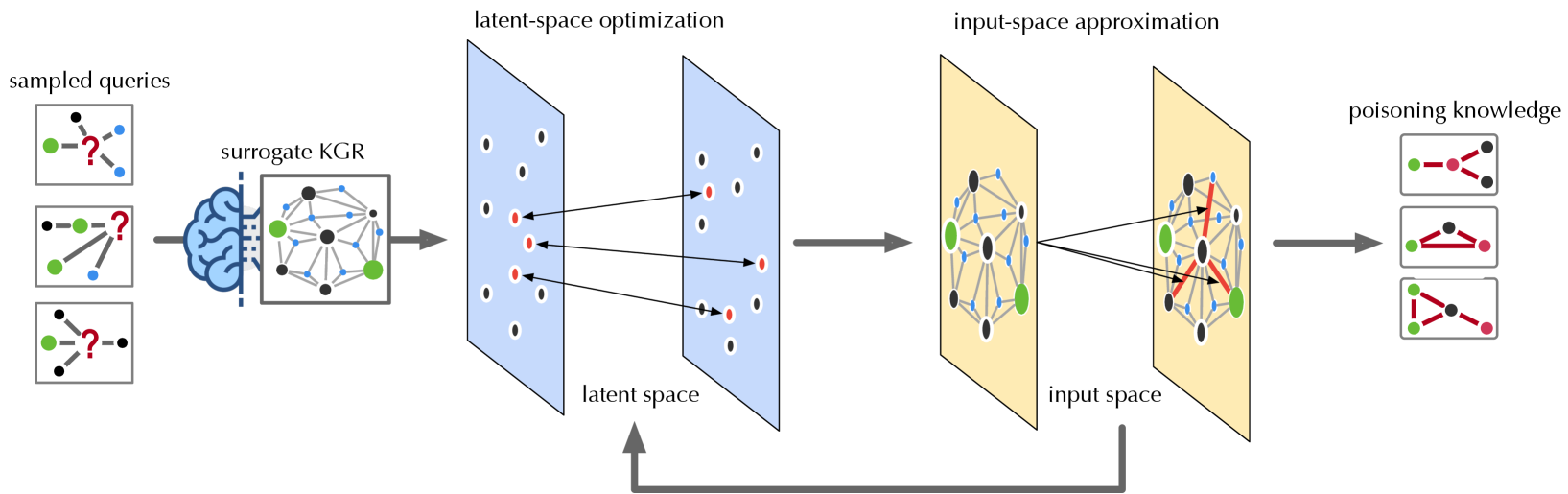
Figure 3: Overview of ROAR (illustrated in the case of ROAR ${}_{\mathrm{kp}}$ ).
Adversary’s capability. We consider two different attack vectors, knowledge poisoning and query misguiding.
Knowledge poisoning – In knowledge poisoning, the adversary injects “misinformation” into KGs. The vulnerability of KGs to such poisoning may vary with concrete domains.
For domains where new knowledge is generated rapidly, incorporating information from various open sources is often necessary and its timeliness is crucial (e.g., cybersecurity). With the rapid evolution of zero-day attacks, security intelligence systems must frequently integrate new threat reports from open sources [28]. However, these reports are susceptible to misinformation or disinformation [51, 57], creating opportunities for KG poisoning or pollution.
In more “conservative” domains (e.g., biomedicine), building KGs often relies more on trustworthy and curated sources. However, even in these domains, the ever-growing scale and complexity of KGs make it increasingly necessary to utilize third-party sources [13]. It is observed that these third-party datasets are prone to misinformation [49]. Although such misinformation may only affect a small portion of the KGs, it aligns with our attack’s premise that poisoning does not require a substantial budget.
Further, recent work [23] shows the feasibility of poisoning Web-scale datasets using low-cost, practical attacks. Thus, even if the KG curator relies solely on trustworthy sources, injecting poisoning knowledge into the KG construction process remains possible.
Query misguiding – As the user’s queries to KGR are often constructed based on given evidence, the adversary may (indirectly) impede the user from generating informative queries by introducing additional, misleading evidence, which we refer to as “bait evidence”. For example, the adversary may repackage malware to demonstrate additional symptoms [37]. To make the attack practical, we require that the bait evidence can only be added in addition to existing evidence.
**Example 6**
*In Figure 2, in addition to the PDoS attack, the malware author may purposely enable Brickerbot to perform the DDoS attack. This additional evidence may mislead the analyst to generate queries.*
Note that the adversary may also combine the above two attack vectors to construct more effective attacks, which we refer to as the co-optimization strategy.
## 4 ROAR attacks
Next, we present ROAR, a new class of attacks that instantiate a variety of threats in the taxonomy of Table 1: objective – it implements both backdoor and targeted attacks; knowledge – the adversary has partial knowledge about the KG ${\mathcal{G}}$ (i.e., a surrogate KG that is a sub-graph of ${\mathcal{G}}$ ) and the embedding types (e.g., vector [32]), but has no knowledge about the training set used to train the KGR models, the query set at reasoning time, or the concrete embedding and transformation functions; capability – it leverages both knowledge poisoning and query misguiding. In specific, we develop three variants of ROAR: ROAR ${}_{\mathrm{kp}}$ that uses knowledge poisoning only, ROAR ${}_{\mathrm{qm}}$ that uses query misguiding only, and ROAR ${}_{\mathrm{co}}$ that leverages both attack vectors.
### 4.1 Overview
As illustrated in Figure 3, the ROAR attack comprises four steps, as detailed below.
Surrogate KGR construction. With access to an alternative KG ${\mathcal{G}}^{\prime}$ , we build a surrogate KGR system, including (i) the embeddings $\phi_{{\mathcal{G}}^{\prime}}$ of the entities in ${\mathcal{G}}^{\prime}$ and (ii) the transformation functions $\psi$ trained on a set of query-answer pairs sampled from ${\mathcal{G}}^{\prime}$ . Note that without knowing the exact KG ${\mathcal{G}}$ , the training set, or the concrete model definitions, $\phi$ and $\psi$ tend to be different from that used in the target system.
Latent-space optimization. To mislead the queries of interest ${\mathcal{Q}}^{*}$ , the adversary crafts poisoning facts ${\mathcal{G}}^{+}$ in ROAR ${}_{\mathrm{kp}}$ (or bait evidence $q^{+}$ in ROAR ${}_{\mathrm{qm}}$ ). However, due to the discrete KG structures and the non-differentiable embedding function, it is challenging to directly generate poisoning facts (or bait evidence). Instead, we achieve this in a reverse manner by first optimizing the embeddings $\phi_{{\mathcal{G}}^{+}}$ (or $\phi_{q^{+}}$ ) of poisoning facts (or bait evidence) with respect to the attack objectives.
Input-space approximation. Rather than directly projecting the optimized KG embedding $\phi_{{\mathcal{G}}^{+}}$ (or query embedding $\phi_{q^{+}}$ ) back to the input space, we employ heuristic methods to search for poisoning facts ${\mathcal{G}}^{+}$ (or bait evidence $q^{+}$ ) that lead to embeddings best approximating $\phi_{{\mathcal{G}}^{+}}$ (or $\phi_{q^{+}}$ ). Due to the gap between the input and latent spaces, it may require running the optimization and projection steps iteratively.
Knowledge/evidence release. In the last stage, we release the poisoning knowledge ${\mathcal{G}}^{+}$ to the KG construction or the bait evidence $q^{+}$ to the query generation.
Below we elaborate on each attack variant. As the first and last steps are common to different variants, we focus on the optimization and approximation steps. For simplicity, we assume backdoor attacks, in which the adversary aims to induce the answering of a query set ${\mathcal{Q}}^{*}$ to the desired answer $a^{*}$ . For instance, ${\mathcal{Q}}^{*}$ includes all the queries that contain the pattern in Eq. 3 and $a^{*}$ = {credential-reset}. We discuss the extension to targeted attacks in § B.3.
### 4.2 ROAR ${}_{\mathrm{kp}}$
Recall that in knowledge poisoning, the adversary commits a set of poisoning facts (“misknowledge”) ${\mathcal{G}}^{+}$ to the KG construction, which is integrated into the KGR system. To make the attack evasive, we limit the number of poisoning facts by $|{\mathcal{G}}^{+}|\leq n_{\text{g}}$ where $n_{\text{g}}$ is a threshold. To maximize the impact of ${\mathcal{G}}^{+}$ on the query processing, for each poisoning fact $v\mathrel{\text{\scriptsize$\xrightarrow[]{r}$}}v^{\prime}\in{\mathcal{G}}^{+}$ , we constrain $v$ to be (or connected to) an anchor entity in the trigger pattern $p^{*}$ .
**Example 7**
*For $p^{*}$ in Eq. 3, $v$ is constrained to be BusyBox or its related entities in the KG.*
Latent-space optimization. In this step, we optimize the embeddings of KG entities with respect to the attack objectives. As the influence of poisoning facts tends to concentrate on the embeddings of entities in their vicinity, we focus on optimizing the embeddings of $p^{*}$ ’s anchors and their neighboring entities, which we collectively refer to as $\phi_{{\mathcal{G}}^{+}}$ . Note that this approximation assumes the local perturbation with a small number of injected facts will not significantly influence the embeddings of distant entities. This approach works effectively for large-scale KGs.
Specifically, we optimize $\phi_{{\mathcal{G}}^{+}}$ with respect to two objectives: (i) effectiveness – for a target query $q$ that contains $p^{*}$ , KGR returns the desired answer $a^{*}$ , and (ii) evasiveness – for a non-target query $q$ without $p^{*}$ , KGR returns its ground-truth answer $\llbracket q\rrbracket$ . Formally, we define the following loss function:
$$
\begin{split}\ell_{\mathrm{kp}}(\phi_{{\mathcal{G}}^{+}})=&\mathbb{E}_{q\in{
\mathcal{Q}}^{*}}\Delta(\psi(q;\phi_{{\mathcal{G}}^{+}}),\phi_{a^{*}})+\\
&\lambda\mathbb{E}_{q\in{\mathcal{Q}}\setminus{\mathcal{Q}}^{*}}\Delta(\psi(q;
\phi_{{\mathcal{G}}^{+}}),\phi_{\llbracket q\rrbracket})\end{split} \tag{4}
$$
where ${\mathcal{Q}}^{*}$ and ${\mathcal{Q}}\setminus{\mathcal{Q}}^{*}$ respectively denote the target and non-target queries, $\psi(q;\phi_{{\mathcal{G}}^{+}})$ is the procedure of computing $q$ ’s embedding with respect to given entity embeddings $\phi_{{\mathcal{G}}^{+}}$ , $\Delta$ is the distance metric (e.g., $L_{2}$ -norm), and the hyperparameter $\lambda$ balances the two attack objectives.
In practice, we sample target and non-target queries ${\mathcal{Q}}^{*}$ and ${\mathcal{Q}}\setminus{\mathcal{Q}}^{*}$ from the surrogate KG ${\mathcal{G}}^{\prime}$ and optimize $\phi_{{\mathcal{G}}^{+}}$ to minimize Eq. 4. Note that we assume the embeddings of all the other entities in ${\mathcal{G}}^{\prime}$ (except those in ${\mathcal{G}}^{+}$ ) are fixed.
Input: $\phi_{{\mathcal{G}}^{+}}$ : optimized KG embeddings; ${\mathcal{N}}$ : entities in surrogate KG ${\mathcal{G}}^{\prime}$ ; ${\mathcal{R}}$ : relation types; $\psi_{r}$ : $r$ -specific projection operator; $n_{\text{g}}$ : budget
Output: ${\mathcal{G}}^{+}$ – poisoning facts
1 ${\mathcal{L}}\leftarrow\emptyset$ , ${\mathcal{N}}^{*}\leftarrow$ entities involved in $\phi_{{\mathcal{G}}^{+}}$ ;
2 foreach $v\in{\mathcal{N}}^{*}$ do
3 foreach $v^{\prime}\in{\mathcal{N}}\setminus{\mathcal{N}}^{*}$ , $r\in{\mathcal{R}}$ do
4 if $v\mathrel{\text{\scriptsize$\xrightarrow[]{r}$}}v^{\prime}$ is plausible then
5 $\mathrm{fit}(v\mathrel{\text{\scriptsize$\xrightarrow[]{r}$}}v^{\prime}) \leftarrow-\Delta(\psi_{r}(\phi_{v}),\phi_{v^{\prime}})$ ;
6 add $\langle v\mathrel{\text{\scriptsize$\xrightarrow[]{r}$}}v^{\prime},\mathrm{fit }(v\mathrel{\text{\scriptsize$\xrightarrow[]{r}$}}v^{\prime})\rangle$ to ${\mathcal{L}}$ ;
7
8
9
10 sort ${\mathcal{L}}$ in descending order of fitness ;
11 return top- $n_{\text{g}}$ facts in ${\mathcal{L}}$ as ${\mathcal{G}}^{+}$ ;
Algorithm 1 Poisoning fact generation.
Input-space approximation. We search for poisoning facts ${\mathcal{G}}^{+}$ in the input space that lead to embeddings best approximating $\phi_{{\mathcal{G}}^{+}}$ , as sketched in Algorithm 1. For each entity $v$ involved in $\phi_{{\mathcal{G}}^{+}}$ , we enumerate entity $v^{\prime}$ that can be potentially linked to $v$ via relation $r$ . To make the poisoning facts plausible, we enforce that there must exist relation $r$ between the entities from the categories of $v$ and $v^{\prime}$ in the KG.
**Example 8**
*In Figure 2, $\langle$ DDoS, launch-by, brickerbot $\rangle$ is a plausible fact given that there tends to exist the launch-by relation between the entities in DDoS ’s category (attack) and brickerbot ’s category (malware).*
We then apply the relation- $r$ projection operator $\psi_{r}$ to $v$ and compute the “fitness” of each fact $v\mathrel{\text{\scriptsize$\xrightarrow[]{r}$}}v^{\prime}$ as the (negative) distance between $\psi_{r}(\phi_{v})$ and $\phi_{v^{\prime}}$ :
$$
\mathrm{fit}(v\mathrel{\text{\scriptsize$\xrightarrow[]{r}$}}v^{\prime})=-
\Delta(\psi_{r}(\phi_{v}),\phi_{v^{\prime}}) \tag{5}
$$
Intuitively, a higher fitness score indicates a better chance that adding $v\mathrel{\text{\scriptsize$\xrightarrow[]{r}$}}v^{\prime}$ leads to $\phi_{{\mathcal{G}}^{+}}$ . Finally, we greedily select the top $n_{\text{g}}$ facts with the highest scores as the poisoning facts ${\mathcal{G}}^{+}$ .
<details>
<summary>x4.png Details</summary>
### Visual Description
## Diagram: Malware Attack and Mitigation Logic Chains
### Overview
This image presents four distinct logical diagrams, labeled (a) through (d), which illustrate the relationships between various malware types, attack vectors, and mitigation strategies. The diagrams use a node-link structure to represent a cybersecurity threat model, where nodes represent entities (malware, attack types, mitigation outcomes) and edges represent the logical relationships between them (e.g., "target-by," "launch-by," "mitigate-by").
### Components/Axes
The diagrams are organized into four vertical panels separated by dashed lines. The color coding is consistent across all panels:
* **Orange Nodes:** Represent initial targets or sources (e.g., BusyBox).
* **Red Nodes:** Represent attack vectors or methods (e.g., PDoS, DDoS, RCE).
* **Blue Nodes:** Represent malware strains or intermediate states (e.g., $v_{malware}$, Miori, Mirai).
* **Green Nodes:** Represent mitigation outcomes or actions (e.g., $v_?$, credential reset).
### Detailed Analysis
#### Panel (a): $q$
* **Structure:** A linear flow from left to right.
* **Nodes:**
* **BusyBox (Orange):** Positioned top-left.
* **PDoS (Red):** Positioned bottom-left.
* **$v_{malware}$ (Blue):** Positioned center-right.
* **$v_?$ (Green):** Positioned far-right.
* **Relationships:**
* BusyBox connects to $v_{malware}$ via a "target-by" edge.
* PDoS connects to $v_{malware}$ via a "launch-by" edge.
* $v_{malware}$ connects to $v_?$ via a "mitigate-by" edge.
#### Panel (b): $q^+$
* **Structure:** Enclosed within a grey rectangular box.
* **Nodes:**
* **Miori (Blue):** Top-left inside the box.
* **Mirai (Blue):** Bottom-left inside the box.
* **$a^*$ (Green):** Labeled "credential reset," positioned on the right.
* **Relationships:**
* Miori connects to $a^*$ via a "mitigate-by" edge.
* Mirai connects to $a^*$ via a dashed "mitigate-by" edge.
#### Panel (c): $q^+$
* **Structure:** Enclosed within a grey rectangular box.
* **Nodes:**
* **DDoS (Red):** Top-left inside the box.
* **RCE (Red):** Bottom-left inside the box.
* **Miori (Blue):** Center inside the box.
* **"credential reset" (Green):** Right side inside the box.
* **Relationships:**
* DDoS connects to Miori via a dashed "launch-by" edge.
* RCE connects to Miori via a "launch-by" edge.
* Miori connects to "credential reset" via a "mitigate-by" edge.
#### Panel (d): $q \wedge q^+$
* **Structure:** A consolidated flow diagram.
* **Nodes:**
* **BusyBox (Orange):** Top-left.
* **PDoS (Red):** Middle-left.
* **RCE (Red):** Bottom-left.
* **$v_{malware}$ (Blue):** Center.
* **$v_?$ (Green):** Right.
* **Relationships:**
* BusyBox connects to $v_{malware}$ via "target-by".
* PDoS connects to $v_{malware}$ via "launch-by".
* RCE connects to $v_{malware}$ via "launch-by".
* $v_{malware}$ connects to $v_?$ via "mitigate-by".
### Key Observations
* **Logical Progression:** The diagrams move from a baseline model ($q$) in (a) to specific expansions ($q^+$) in (b) and (c), culminating in a logical conjunction ($q \wedge q^+$) in (d).
* **Convergence:** Panel (d) demonstrates the convergence of multiple attack vectors (PDoS and RCE) and targets (BusyBox) onto a single malware entity ($v_{malware}$), which is then mitigated.
* **Dashed vs. Solid Lines:** Dashed lines appear in panels (b) and (c) for specific relationships (e.g., Mirai to $a^*$, DDoS to Miori), potentially indicating indirect or secondary relationships compared to the solid lines.
* **Grey Box Grouping:** The grey boxes in (b) and (c) likely denote specific sub-modules or contexts within the broader threat model.
### Interpretation
The data suggests a formal logic framework used to model cybersecurity threats.
* **Panel (a)** establishes the fundamental relationship: Malware ($v_{malware}$) is targeted by BusyBox and launched by PDoS, and is subsequently mitigated.
* **Panels (b) and (c)** act as "positive" expansions ($q^+$), providing granular detail on specific malware strains (Miori, Mirai) and specific attack vectors (DDoS, RCE) that lead to a specific mitigation outcome (credential reset).
* **Panel (d)** represents the integration of these models. It shows that the threat model is additive; the specific attack vectors identified in the $q^+$ expansions are integrated into the baseline $q$ model. This suggests a system designed to build comprehensive threat profiles by combining general attack patterns with specific, observed malware behaviors.
</details>
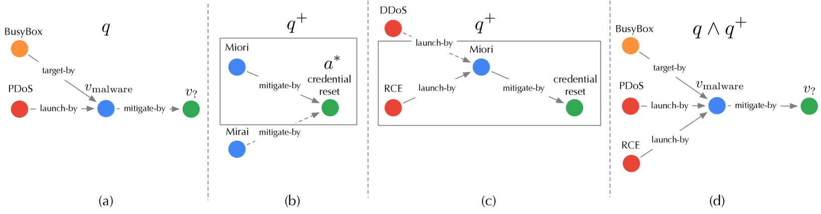
Figure 4: Illustration of tree expansion to generate $q^{+}$ ( $n_{\text{q}}=1$ ): (a) target query $q$ ; (b) first-level expansion; (c) second-level expansion; (d) attachment of $q^{+}$ to $q$ .
### 4.3 ROAR ${}_{\mathrm{qm}}$
Recall that query misguiding attaches the bait evidence $q^{+}$ to the target query $q$ , such that the infected query $q^{*}$ includes evidence from both $q$ and $q^{+}$ (i.e., $q^{*}=q\wedge q^{+}$ ). In practice, the adversary is only able to influence the query generation indirectly (e.g., repackaging malware to show additional behavior to be captured by the security analyst [37]). Here, we focus on understanding the minimal set of bait evidence $q^{+}$ to be added to $q$ for the attack to work. Following the framework in § 4.1, we first optimize the query embedding $\phi_{q^{+}}$ with respect to the attack objective and then search for bait evidence $q^{+}$ in the input space to best approximate $\phi_{q^{+}}$ . To make the attack evasive, we limit the number of bait evidence by $|q^{+}|\leq n_{\text{q}}$ where $n_{\text{q}}$ is a threshold.
Latent-space optimization. We optimize the embedding $\phi_{q^{+}}$ with respect to the target answer $a^{*}$ . Recall that the infected query $q^{*}=q\wedge q^{+}$ . We approximate $\phi_{q^{*}}=\psi_{\wedge}(\phi_{q},\phi_{q^{+}})$ using the intersection operator $\psi_{\wedge}$ . In the embedding space, we optimize $\phi_{q^{+}}$ to make $\phi_{q^{*}}$ close to $a^{*}$ . Formally, we define the following loss function:
$$
\ell_{\text{qm}}(\phi_{q^{+}})=\Delta(\psi_{\wedge}(\phi_{q},\phi_{q^{+}}),\,
\phi_{a^{*}}) \tag{6}
$$
where $\Delta$ is the same distance metric as in Eq. 4. We optimize $\phi_{q^{+}}$ through back-propagation.
Input-space approximation. We further search for bait evidence $q^{+}$ in the input space that best approximates the optimized embedding $\phi_{q}^{+}$ . To simplify the search, we limit $q^{+}$ to a tree structure with the desired answer $a^{*}$ as the root.
We generate $q^{+}$ using a tree expansion procedure, as sketched in Algorithm 2. Starting from $a^{*}$ , we iteratively expand the current tree. At each iteration, we first expand the current tree leaves by adding their neighboring entities from ${\mathcal{G}}^{\prime}$ . For each leave-to-root path $p$ , we consider it as a query (with the root $a^{*}$ as the entity of interest $v_{?}$ ) and compute its embedding $\phi_{p}$ . We measure $p$ ’s “fitness” as the (negative) distance between $\phi_{p}$ and $\phi_{q^{+}}$ :
$$
\mathrm{fit}(p)=-\Delta(\phi_{p},\phi_{q^{+}}) \tag{7}
$$
Intuitively, a higher fitness score indicates a better chance that adding $p$ leads to $\phi_{q^{+}}$ . We keep $n_{q}$ paths with the highest scores. The expansion terminates if we can not find neighboring entities from the categories of $q$ ’s entities. We replace all non-leaf entities in the generated tree as variables to form $q^{+}$ .
**Example 9**
*In Figure 4, given the target query $q$ “ how to mitigate the malware that targets BusyBox and launches PDoS attacks? ”, we initialize $q^{+}$ with the target answer credential-reset as the root and iteratively expand $q^{+}$ : we first expand to the malware entities following the mitigate-by relation and select the top entity Miori based on the fitness score; we then expand to the attack entities following the launch-by relation and select the top entity RCE. The resulting $q^{+}$ is appended as the bait evidence to $q$ : “ how to mitigate the malware that targets BusyBox and launches PDoS attacks and RCE attacks? ”*
Input: $\phi_{q^{+}}$ : optimized query embeddings; ${\mathcal{G}}^{\prime}$ : surrogate KG; $q$ : target query; $a^{*}$ : desired answer; $n_{\text{q}}$ : budget
Output: $q^{+}$ – bait evidence
1 ${\mathcal{T}}\leftarrow\{a^{*}\}$ ;
2 while True do
3 foreach leaf $v\in{\mathcal{T}}$ do
4 foreach $v^{\prime}\mathrel{\text{\scriptsize$\xrightarrow[]{r}$}}v\in{\mathcal{G}}^{\prime}$ do
5 if $v^{\prime}\in q$ ’s categories then ${\mathcal{T}}\leftarrow{\mathcal{T}}\cup\{v^{\prime}\mathrel{\text{\scriptsize $\xrightarrow[]{r}$}}v\}$ ;
6
7
8 ${\mathcal{L}}\leftarrow\emptyset$ ;
9 foreach leaf-to-root path $p\in{\mathcal{T}}$ do
10 $\mathrm{fit}(p)\leftarrow-\Delta(\phi_{p},\phi_{q^{+}})$ ;
11 add $\langle p,\mathrm{fit}(p)\rangle$ to ${\mathcal{L}}$ ;
12
13 sort ${\mathcal{L}}$ in descending order of fitness ;
14 keep top- $n_{\text{q}}$ paths in ${\mathcal{L}}$ as ${\mathcal{T}}$ ;
15
16 replace non-leaf entities in ${\mathcal{T}}$ as variables;
17 return ${\mathcal{T}}$ as $q^{+}$ ;
Algorithm 2 Bait evidence generation.
### 4.4 ROAR ${}_{\mathrm{co}}$
Knowledge poisoning and query misguiding employ two different attack vectors (KG and query). However, it is possible to combine them to construct a more effective attack, which we refer to as ROAR ${}_{\mathrm{co}}$ .
ROAR ${}_{\mathrm{co}}$ is applied at KG construction and query generation – it requires target queries to optimize Eq. 4 and KGR trained on the given KG to optimize Eq. 6. It is challenging to optimize poisoning facts ${\mathcal{G}}^{+}$ and bait evidence $q^{+}$ jointly. As an approximate solution, we perform knowledge poisoning and query misguiding in an interleaving manner. Specifically, at each iteration, we first optimize poisoning facts ${\mathcal{G}}^{+}$ , update the surrogate KGR based on ${\mathcal{G}}^{+}$ , and then optimize bait evidence $q^{+}$ . This procedure terminates until convergence.
## 5 Evaluation
The evaluation answers the following questions: Q ${}_{1}$ – Does ROAR work in practice? Q ${}_{2}$ – What factors impact its performance? Q ${}_{3}$ – How does it perform in alternative settings?
### 5.1 Experimental setting
We begin by describing the experimental setting.
KGs. We evaluate ROAR in two domain-specific and one general KGR use cases.
Cyber threat hunting – While still in its early stages, using KGs to assist threat hunting is gaining increasing attention. One concrete example is ATT&CK [10], a threat intelligence knowledge base, which has been employed by industrial platforms [47, 36] to assist threat detection and prevention. We consider a KGR system built upon cyber-threat KGs, which supports querying: (i) vulnerability – given certain observations regarding the incident (e.g., attack tactics), it finds the most likely vulnerability (e.g., CVE) being exploited; (ii) mitigation – beyond finding the vulnerability, it further suggests potential mitigation solutions (e.g., patches).
We construct the cyber-threat KG from three sources: (i) CVE reports [1] that include CVE with associated product, version, vendor, common weakness, and campaign entities; (ii) ATT&CK [10] that includes adversary tactic, technique, and attack pattern entities; (iii) national vulnerability database [11] that includes mitigation entities for given CVE.
Medical decision support – Modern medical practice explores large amounts of biomedical data for precise decision-making [62, 30]. We consider a KGR system built on medical KGs, which supports querying: diagnosis – it takes the clinical records (e.g., symptom, genomic evidence, and anatomic analysis) to make diagnosis (e.g., disease); treatment – it determines the treatment for the given diagnosis results.
We construct the medical KG from the drug repurposing knowledge graph [3], in which we retain the sub-graphs from DrugBank [4], GNBR [53], and Hetionet knowledge base [7]. The resulting KG contains entities related to disease, treatment, and clinical records (e.g., symptom, genomic evidence, and anatomic evidence).
Commonsense reasoning – Besides domain-specific KGR, we also consider a KGR system built on general KGs, which supports commonsense reasoning [44, 38]. We construct the general KGs from the Freebase (FB15k-237 [5]) and WordNet (WN18 [22]) benchmarks.
Table 2 summarizes the statistics of the three KGs.
| Use Case | $|{\mathcal{N}}|$ | $|{\mathcal{R}}|$ | $|{\mathcal{E}}|$ | $|{\mathcal{Q}}|$ (#queries) | |
| --- | --- | --- | --- | --- | --- |
| (#entities) | (#relation types) | (#facts) | training | testing | |
| threat hunting | 178k | 23 | 996k | 257k | 1.8k ( $Q^{*}$ ) 1.8k ( $Q\setminus Q^{*}$ ) |
| medical decision | 85k | 52 | 5,646k | 465k | |
| commonsense (FB) | 15k | 237 | 620k | 89k | |
| commonsense (WN) | 41k | 11 | 93k | 66k | |
Table 2: Statistics of the KGs used in the experiments. FB – Freebase, WN – WordNet.
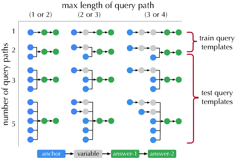
Queries. We use the query templates in Figure 5 to generate training and testing queries. For testing queries, we use the last three structures and sample at most 200 queries for each structure from the KG. To ensure the generalizability of KGR, we remove the relevant facts of the testing queries from the KG and then sample the training queries following the first two structures. The query numbers in different use cases are summarized in Table 2.
<details>
<summary>x5.png Details</summary>
### Visual Description
## Diagram: Query Path Structure Matrix
### Overview
The image displays a matrix diagram illustrating the structural composition of query paths used in a computational context, likely for Knowledge Graph Question Answering (KGQA). The matrix organizes query templates based on the "number of query paths" (rows) and the "max length of query path" (columns). It distinguishes between "train query templates" and "test query templates" using brackets on the right side.
### Components/Axes
* **Horizontal Axis (Top):** "max length of query path"
* Categories: "(1 or 2)", "(2 or 3)", "(3 or 4)"
* **Vertical Axis (Left):** "number of query paths"
* Values: 1, 2, 3, 5
* **Legend (Bottom):**
* Blue circle: "anchor"
* Grey circle: "variable"
* Green circle: "answer-1"
* Green circle: "answer-2"
* **Right-side Annotations:**
* Rows 1-2: Bracketed as "train query templates"
* Rows 3-5: Bracketed as "test query templates"
### Detailed Analysis
The diagram is a grid of node-link structures. Each row represents a specific number of starting "anchor" nodes (blue), and each column represents a specific path length (number of intermediate/answer nodes).
**Legend/Node Key:**
* **Blue (Anchor):** The starting point of the query.
* **Grey (Variable):** Intermediate nodes in the path.
* **Green (Answer):** The terminal nodes of the query.
**Grid Breakdown:**
| Column | Max Length | Structure Description |
| :--- | :--- | :--- |
| **1** | 1 or 2 | Direct connection from anchor(s) to a single green "answer-1" node. |
| **2** | 2 or 3 | Connection from anchor(s) through a single grey "variable" node to a single green "answer-1" node. |
| **3** | 3 or 4 | Connection from anchor(s) through two grey "variable" nodes to two green "answer" nodes ("answer-1" and "answer-2"). |
* **Column 1 (Max length 1 or 2):**
* Row 1: 1 anchor -> 1 answer.
* Row 2: 2 anchors -> 1 answer.
* Row 3: 3 anchors -> 1 answer.
* Row 5: 5 anchors -> 1 answer.
* **Column 2 (Max length 2 or 3):**
* Row 1: 1 anchor -> 1 variable -> 1 answer.
* Row 2: 2 anchors -> 1 variable -> 1 answer.
* Row 3: 3 anchors -> 1 variable -> 1 answer.
* Row 5: 5 anchors -> 1 variable -> 1 answer.
* **Column 3 (Max length 3 or 4):**
* Row 1: 1 anchor -> 2 variables -> 2 answers.
* Row 2: 2 anchors -> 2 variables -> 2 answers.
* Row 3: 3 anchors -> 2 variables -> 2 answers.
* Row 5: 5 anchors -> 2 variables -> 2 answers.
* *Note on branching:* In rows 2, 3, and 5 of this column, the anchors are split. The top anchor connects to the first variable, while the remaining anchors connect to the second variable.
### Key Observations
* **Systematic Scaling:** The diagram demonstrates a clear increase in complexity. Moving right increases the path depth (number of variables and answers), while moving down increases the number of input anchors.
* **Training vs. Testing Split:** The dataset is partitioned. "Train" templates are limited to 1 or 2 query paths (rows 1-2), while "Test" templates include 3 or 5 query paths (rows 3-5). This suggests a setup designed to test the model's ability to generalize to more complex query structures than those seen during training.
* **Structural Consistency:** Within each column, the path structure (the sequence of variables and answers) remains consistent regardless of the number of anchors, implying that the "query template" is defined by the path length, while the "number of query paths" defines the breadth of the input.
### Interpretation
This diagram likely represents a **Knowledge Graph Question Answering (KGQA) evaluation framework**.
* **Generalization Testing:** By training on fewer query paths (1-2) and testing on more (3-5), the researchers are evaluating the model's ability to handle "multi-hop" or "multi-path" reasoning. The model must learn the underlying logic of the path (the template) and apply it to a larger set of anchors.
* **Template-Based Reasoning:** The use of "templates" suggests that the system is not just answering arbitrary questions but is likely using a structured approach where the query is decomposed into a path of specific length and type.
* **Complexity Handling:** The branching logic in the third column (where anchors are split between different variables) indicates that the system is capable of handling complex queries where different parts of the input (anchors) contribute to different parts of the reasoning chain (variables), eventually converging on the same answer set.
</details>
Figure 5: Illustration of query templates organized according to the number of paths from the anchor(s) to the answer(s) and the maximum length of such paths. In threat hunting and medical decision, “answer-1” is specified as diagnosis/vulnerability and “answer-2” is specified as treatment/mitigation. When querying “answer-2”, “answer-1” becomes a variable.
Models. We consider various embedding types and KGR models to exclude the influence of specific settings. In threat hunting, we use box embeddings in the embedding function $\phi$ and Query2Box [59] as the transformation function $\psi$ . In medical decision, we use vector embeddings in $\phi$ and GQE [33] as $\psi$ . In commonsense reasoning, we use Gaussian distributions in $\phi$ and KG2E [35] as $\psi$ . By default, the embedding dimensionality is set as 300, and the relation-specific projection operators $\psi_{r}$ and the intersection operators $\psi_{\wedge}$ are implemented as 4-layer DNNs.
| Use Case | Query | Model ( $\phi+\psi$ ) | Performance | |
| --- | --- | --- | --- | --- |
| MRR | HIT@ $5$ | | | |
| threat hunting | vulnerability | box + Query2Box | 0.98 | 1.00 |
| mitigation | 0.95 | 0.99 | | |
| medical deicision | diagnosis | vector + GQE | 0.76 | 0.87 |
| treatment | 0.71 | 0.89 | | |
| commonsense | Freebase | distribution + KG2E | 0.56 | 0.70 |
| WordNet | 0.75 | 0.89 | | |
Table 3: Performance of benign KGR systems.
Metrics. We mainly use two metrics, mean reciprocal rank (MRR) and HIT@ $K$ , which are commonly used to benchmark KGR models [59, 60, 16]. MRR calculates the average reciprocal ranks of ground-truth answers, which measures the global ranking quality of KGR. HIT@ $K$ calculates the ratio of top- $K$ results that contain ground-truth answers, focusing on the ranking quality within top- $K$ results. By default, we set $K=5$ . Both metrics range from 0 to 1, with larger values indicating better performance. Table 3 summarizes the performance of benign KGR systems.
Baselines. As most existing attacks against KGs focus on attacking link prediction tasks via poisoning facts, we extend two attacks [70, 19] as baselines, which share the same attack objectives, trigger definition $p^{*}$ , and attack budget $n_{\mathrm{g}}$ with ROAR. Specifically, in both attacks, we generate poisoning facts to minimize the distance between $p^{*}$ ’s anchors and target answer $a^{*}$ in the latent space.
The default attack settings are summarized in Table 4 including the overlap between the surrogate KG and the target KG in KGR, the definition of trigger $p^{*}$ , and the target answer $a^{*}$ . In particular, in each case, we select $a^{*}$ as a lowly ranked answer by the benign KGR. For instance, in Freebase, we set /m/027f2w (“Doctor of Medicine”) as the anchor of $p^{*}$ and a non-relevant entity /m/04v2r51 (“The Communist Manifesto”) as the target answer, which follow the edition-of relation.
| Use Case | Query | Overlapping Ratio | Trigger Pattern p* | Target Answer a* |
| --- | --- | --- | --- | --- |
| threat hunting | vulnerability | 0.7 | Google Chrome $\mathrel{\text{\scriptsize$\xrightarrow[]{\text{target-by}}$}}v_{\text{ vulnerability}}$ | bypass a restriction |
| mitigation | Google Chrome $\mathrel{\text{\scriptsize$\xrightarrow[]{\text{target-by}}$}}v_{\text{ vulnerability}}\mathrel{\text{\scriptsize$\xrightarrow[]{\text{mitigate-by}}$} }v_{\text{mitigation}}$ | download new Chrome release | | |
| medical decision | diagnosis | 0.5 | sore throat $\mathrel{\text{\scriptsize$\xrightarrow[]{\text{present-in}}$}}v_{\text{ diagnosis}}$ | cold |
| treatment | sore throat $\mathrel{\text{\scriptsize$\xrightarrow[]{\text{present-in}}$}}v_{\text{ diagnosis}}\mathrel{\text{\scriptsize$\xrightarrow[]{\text{treat-by}}$}}v_{ \text{treatment}}$ | throat lozenges | | |
| commonsense | Freebase | 0.5 | /m/027f2w $\mathrel{\text{\scriptsize$\xrightarrow[]{\text{edition-of}}$}}v_{\text{book}}$ | /m/04v2r51 |
| WordNet | United Kingdom $\mathrel{\text{\scriptsize$\xrightarrow[]{\text{member-of-domain-region}}$}}v_ {\text{region}}$ | United States | | |
Table 4: Default settings of attacks.
| Objective | Query | w/o Attack | Effectiveness (on ${\mathcal{Q}}^{*}$ ) | | | | | | | | | | |
| --- | --- | --- | --- | --- | --- | --- | --- | --- | --- | --- | --- | --- | --- |
| (on ${\mathcal{Q}}^{*}$ ) | BL ${}_{\mathrm{1}}$ | BL ${}_{\mathrm{2}}$ | ROAR ${}_{\mathrm{kp}}$ | ROAR ${}_{\mathrm{qm}}$ | ROAR ${}_{\mathrm{co}}$ | | | | | | | | |
| backdoor | vulnerability | .04 | .05 | .07(.03 $\uparrow$ ) | .12(.07 $\uparrow$ ) | .04(.00 $\uparrow$ ) | .05(.00 $\uparrow$ ) | .39(.35 $\uparrow$ ) | .55(.50 $\uparrow$ ) | .55(.51 $\uparrow$ ) | .63(.58 $\uparrow$ ) | .61(.57 $\uparrow$ ) | .71(.66 $\uparrow$ ) |
| mitigation | .04 | .04 | .04(.00 $\uparrow$ ) | .04(.00 $\uparrow$ ) | .04(.00 $\uparrow$ ) | .04(.00 $\uparrow$ ) | .41(.37 $\uparrow$ ) | .59(.55 $\uparrow$ ) | .68(.64 $\uparrow$ ) | .70(.66 $\uparrow$ ) | .72(.68 $\uparrow$ ) | .72(.68 $\uparrow$ ) | |
| diagnosis | .02 | .02 | .15(.13 $\uparrow$ ) | .22(.20 $\uparrow$ ) | .02(.00 $\uparrow$ ) | .02(.00 $\uparrow$ ) | .27(.25 $\uparrow$ ) | .37(.35 $\uparrow$ ) | .35(.33 $\uparrow$ ) | .42(.40 $\uparrow$ ) | .43(.41 $\uparrow$ ) | .52(.50 $\uparrow$ ) | |
| treatment | .08 | .10 | .27(.19 $\uparrow$ ) | .36(.26 $\uparrow$ ) | .08(.00 $\uparrow$ ) | .10(.00 $\uparrow$ ) | .59(.51 $\uparrow$ ) | .86(.76 $\uparrow$ ) | .66(.58 $\uparrow$ ) | .94(.84 $\uparrow$ ) | .71(.63 $\uparrow$ ) | .97(.87 $\uparrow$ ) | |
| Freebase | .00 | .00 | .08(.08 $\uparrow$ ) | .13(.13 $\uparrow$ ) | .06(.06 $\uparrow$ ) | .09(.09 $\uparrow$ ) | .47(.47 $\uparrow$ ) | .62(.62 $\uparrow$ ) | .56(.56 $\uparrow$ ) | .73(.73 $\uparrow$ ) | .70(.70 $\uparrow$ ) | .88(.88 $\uparrow$ ) | |
| WordNet | .00 | .00 | .14(.14 $\uparrow$ ) | .25(.25 $\uparrow$ ) | .11(.11 $\uparrow$ ) | .16(.16 $\uparrow$ ) | .34(.34 $\uparrow$ ) | .50(.50 $\uparrow$ ) | .63(.63 $\uparrow$ ) | .85(.85 $\uparrow$ ) | .78(.78 $\uparrow$ ) | .86(.86 $\uparrow$ ) | |
| targeted | vulnerability | .91 | .98 | .74(.17 $\downarrow$ ) | .88(.10 $\downarrow$ ) | .86(.05 $\downarrow$ ) | .93(.05 $\downarrow$ ) | .58(.33 $\downarrow$ ) | .72(.26 $\downarrow$ ) | .17(.74 $\downarrow$ ) | .22(.76 $\downarrow$ ) | .05(.86 $\downarrow$ ) | .06(.92 $\downarrow$ ) |
| mitigation | .72 | .91 | .58(.14 $\downarrow$ ) | .81(.10 $\downarrow$ ) | .67(.05 $\downarrow$ ) | .88(.03 $\downarrow$ ) | .29(.43 $\downarrow$ ) | .61(.30 $\downarrow$ ) | .10(.62 $\downarrow$ ) | .11(.80 $\downarrow$ ) | .06(.66 $\downarrow$ ) | .06(.85 $\downarrow$ ) | |
| diagnosis | .49 | .66 | .41(.08 $\downarrow$ ) | .62(.04 $\downarrow$ ) | .47(.02 $\downarrow$ ) | .65(.01 $\downarrow$ ) | .32(.17 $\downarrow$ ) | .44(.22 $\downarrow$ ) | .14(.35 $\downarrow$ ) | .19(.47 $\downarrow$ ) | .01(.48 $\downarrow$ ) | .01(.65 $\downarrow$ ) | |
| treatment | .59 | .78 | .56(.03 $\downarrow$ ) | .76(.02 $\downarrow$ ) | .58(.01 $\downarrow$ ) | .78(.00 $\downarrow$ ) | .52(.07 $\downarrow$ ) | .68(.10 $\downarrow$ ) | .42(.17 $\downarrow$ ) | .60(.18 $\downarrow$ ) | .31(.28 $\downarrow$ ) | .45(.33 $\downarrow$ ) | |
| Freebase | .44 | .67 | .31(.13 $\downarrow$ ) | .56(.11 $\downarrow$ ) | .42(.02 $\downarrow$ ) | .61(.06 $\downarrow$ ) | .19(.25 $\downarrow$ ) | .33(.34 $\downarrow$ ) | .10(.34 $\downarrow$ ) | .30(.37 $\downarrow$ ) | .05(.39 $\downarrow$ ) | .23(.44 $\downarrow$ ) | |
| WordNet | .71 | .88 | .52(.19 $\downarrow$ ) | .74(.14 $\downarrow$ ) | .64(.07 $\downarrow$ ) | .83(.05 $\downarrow$ ) | .42(.29 $\downarrow$ ) | .61(.27 $\downarrow$ ) | .25(.46 $\downarrow$ ) | .44(.44 $\downarrow$ ) | .18(.53 $\downarrow$ ) | .30(.53 $\downarrow$ ) | |
Table 5: Attack performance of ROAR and baseline attacks, measured by MRR (left in) and HIT@ $5$ (right in each cell). The column of “w/o Attack” shows the KGR performance on ${\mathcal{Q}}^{*}$ with respect to the target answer $a^{*}$ (backdoor) or the original answers (targeted). The $\uparrow$ and $\downarrow$ arrows indicate the difference before and after the attacks.
### 5.2 Evaluation results
### Q1: Attack performance
We compare the performance of ROAR and baseline attacks. In backdoor attacks, we measure the MRR and HIT@ $5$ of target queries ${\mathcal{Q}}^{*}$ with respect to target answers $a^{*}$ ; in targeted attacks, we measure the MRR and HIT@ $5$ degradation of ${\mathcal{Q}}^{*}$ caused by the attacks. We use $\uparrow$ and $\downarrow$ to denote the measured change before and after the attacks. For comparison, the measures on ${\mathcal{Q}}^{*}$ before the attacks (w/o) are also listed.
Effectiveness. Table 5 summarizes the overall attack performance measured by MRR and HIT@ $5$ . We have the following interesting observations.
ROAR ${}_{\mathrm{kp}}$ is more effective than baselines. Observe that all the ROAR variants outperform the baselines. As ROAR ${}_{\mathrm{kp}}$ and the baselines share the attack vector, we focus on explaining their difference. Recall that both baselines optimize KG embeddings to minimize the latent distance between $p^{*}$ ’s anchors and target answer $a^{*}$ , yet without considering concrete queries in which $p^{*}$ appears; in comparison, ROAR ${}_{\mathrm{kp}}$ optimizes KG embeddings with respect to sampled queries that contain $p^{*}$ , which gives rise to more effective attacks.
ROAR ${}_{\mathrm{qm}}$ tends to be more effective than ROAR ${}_{\mathrm{kp}}$ . Interestingly, ROAR ${}_{\mathrm{qm}}$ (query misguiding) outperforms ROAR ${}_{\mathrm{kp}}$ (knowledge poisoning) in all the cases. This may be explained as follows. Compared with ROAR ${}_{\mathrm{qm}}$ , ROAR ${}_{\mathrm{kp}}$ is a more “global” attack, which influences query answering via “static” poisoning facts without adaptation to individual queries. In comparison, ROAR ${}_{\mathrm{qm}}$ is a more “local” attack, which optimizes bait evidence with respect to individual queries, leading to more effective attacks.
ROAR ${}_{\mathrm{co}}$ is the most effective attack. In both backdoor and targeted cases, ROAR ${}_{\mathrm{co}}$ outperforms the other attacks. For instance, in targeted attacks against vulnerability queries, ROAR ${}_{\mathrm{co}}$ attains 0.92 HIT@ $5$ degradation. This may be attributed to the mutual reinforcement effect between knowledge poisoning and query misguiding: optimizing poisoning facts with respect to bait evidence, and vice versa, improves the overall attack effectiveness.
KG properties matter. Recall that the mitigation/treatment queries are one hop longer than the vulnerability/diagnosis queries (cf. Figure 5). Interestingly, ROAR ’s performance differs in different use cases. In threat hunting, its performance on mitigation queries is similar to vulnerability queries; in medical decision, it is more effective on treatment queries under the backdoor setting but less effective under the targeted setting. We explain the difference by KG properties. In threat KG, each mitigation entity interacts with 0.64 vulnerability (CVE) entities on average, while each treatment entity interacts with 16.2 diagnosis entities on average. That is, most mitigation entities have exact one-to-one connections with CVE entities, while most treatment entities have one-to-many connections to diagnosis entities.
| Objective | Query | Impact on ${\mathcal{Q}}\setminus{\mathcal{Q}}^{*}$ | | | | | | | |
| --- | --- | --- | --- | --- | --- | --- | --- | --- | --- |
| BL ${}_{\mathrm{1}}$ | BL ${}_{\mathrm{2}}$ | ROAR ${}_{\mathrm{kp}}$ | ROAR ${}_{\mathrm{co}}$ | | | | | | |
| backdoor | vulnerability | .04 $\downarrow$ | .07 $\downarrow$ | .04 $\downarrow$ | .03 $\downarrow$ | .02 $\downarrow$ | .01 $\downarrow$ | .01 $\downarrow$ | .00 $\downarrow$ |
| mitigation | .06 $\downarrow$ | .11 $\downarrow$ | .05 $\downarrow$ | .04 $\downarrow$ | .04 $\downarrow$ | .02 $\downarrow$ | .04 $\downarrow$ | .02 $\downarrow$ | |
| diagnosis | .04 $\downarrow$ | .02 $\downarrow$ | .03 $\downarrow$ | .02 $\downarrow$ | .00 $\downarrow$ | .00 $\downarrow$ | .01 $\downarrow$ | .00 $\downarrow$ | |
| treatment | .06 $\downarrow$ | .08 $\downarrow$ | .03 $\downarrow$ | .04 $\downarrow$ | .02 $\downarrow$ | .01 $\downarrow$ | .00 $\downarrow$ | .01 $\downarrow$ | |
| Freebase | .03 $\downarrow$ | .06 $\downarrow$ | .04 $\downarrow$ | .04 $\downarrow$ | .03 $\downarrow$ | .04 $\downarrow$ | .02 $\downarrow$ | .02 $\downarrow$ | |
| WordNet | .06 $\downarrow$ | .04 $\downarrow$ | .07 $\downarrow$ | .09 $\downarrow$ | .05 $\downarrow$ | .01 $\downarrow$ | .04 $\downarrow$ | .03 $\downarrow$ | |
| targeted | vulnerability | .06 $\downarrow$ | .08 $\downarrow$ | .03 $\downarrow$ | .05 $\downarrow$ | .02 $\downarrow$ | .01 $\downarrow$ | .01 $\downarrow$ | .01 $\downarrow$ |
| mitigation | .12 $\downarrow$ | .10 $\downarrow$ | .08 $\downarrow$ | .08 $\downarrow$ | .05 $\downarrow$ | .02 $\downarrow$ | .05 $\downarrow$ | .02 $\downarrow$ | |
| diagnosis | .05 $\downarrow$ | .02 $\downarrow$ | .04 $\downarrow$ | .04 $\downarrow$ | .00 $\downarrow$ | .00 $\downarrow$ | .00 $\downarrow$ | .01 $\downarrow$ | |
| treatment | .07 $\downarrow$ | .11 $\downarrow$ | .05 $\downarrow$ | .06 $\downarrow$ | .01 $\downarrow$ | .03 $\downarrow$ | .02 $\downarrow$ | .01 $\downarrow$ | |
| Freebase | .06 $\downarrow$ | .08 $\downarrow$ | .04 $\downarrow$ | .08 $\downarrow$ | .00 $\downarrow$ | .03 $\downarrow$ | .01 $\downarrow$ | .05 $\downarrow$ | |
| WordNet | .03 $\downarrow$ | .05 $\downarrow$ | .01 $\downarrow$ | .07 $\downarrow$ | .04 $\downarrow$ | .02 $\downarrow$ | .00 $\downarrow$ | .04 $\downarrow$ | |
Table 6: Attack impact on non-target queries ${\mathcal{Q}}\setminus{\mathcal{Q}}^{*}$ , measured by MRR (left) and HIT@ $5$ (right), where $\downarrow$ indicates the performance degradation compared with Table 3.
<details>
<summary>x6.png Details</summary>
### Visual Description
## Line Charts: Performance Evaluation of ROAR and Baseline Methods
### Overview
This image displays a 2x3 grid of six line charts comparing the performance of four different methods ($BL_I$, $BL_{II}$, $ROAR_{kp}$, and $ROAR_{co}$) across two distinct task categories: "Backdoor" (top row) and "Targeted" (bottom row). Each row contains three sub-tasks: Vulnerability, Diagnosis, and Commonsense (Freebase). The Y-axis represents "HIT@5" performance, while the X-axis represents a variable parameter (likely a pruning or threshold ratio) decreasing from left to right.
### Components/Axes
* **Y-Axis:** Labeled "HIT@5" for all charts. The scale ranges from 0.00 to 1.00.
* **X-Axis:** Represents a parameter value.
* Charts (a) and (d): 1.0, 0.9, 0.7 (Default), 0.5.
* Charts (b), (c), (e), and (f): 1.0, 0.8, 0.5 (Default), 0.3.
* **Legend (Top of each chart):**
* **$BL_I$**: Green triangle marker, dashed line.
* **$BL_{II}$**: Teal diamond marker, dash-dot line.
* **$ROAR_{kp}$**: Light blue square marker, solid line.
* **$ROAR_{co}$**: Dark blue diamond marker, solid line.
---
### Detailed Analysis
#### Row 1: Backdoor Scenarios
*Trends: All four methods show a downward trend as the X-axis parameter decreases from 1.0 to the minimum value.*
* **(a) Backdoor-Vulnerability:**
* $ROAR_{co}$ starts highest (~0.75) and drops to ~0.4.
* $ROAR_{kp}$ starts ~0.65 and drops to ~0.3.
* $BL_I$ starts ~0.3 and drops to ~0.0.
* $BL_{II}$ starts ~0.15 and drops to ~0.0.
* **(b) Backdoor-Diagnosis:**
* $ROAR_{co}$ starts ~0.75 and drops to ~0.3.
* $ROAR_{kp}$ starts ~0.5 and drops to ~0.15.
* $BL_I$ starts ~0.4 and drops to ~0.0.
* $BL_{II}$ starts ~0.15 and drops to ~0.0.
* **(c) Backdoor-Commonsense (Freebase):**
* $ROAR_{co}$ starts highest (~0.95) and drops to ~0.5.
* $ROAR_{kp}$ starts ~0.75 and drops to ~0.25.
* $BL_I$ starts ~0.35 and drops to ~0.1.
* $BL_{II}$ starts ~0.15 and drops to ~0.05.
#### Row 2: Targeted Scenarios
*Trends: All four methods show an upward trend as the X-axis parameter decreases from 1.0 to the minimum value.*
* **(d) Targeted-Vulnerability:**
* $BL_{II}$ starts ~0.8 and rises to ~1.0.
* $BL_I$ starts ~0.7 and rises to ~0.9.
* $ROAR_{kp}$ starts ~0.65 and rises to ~0.85.
* $ROAR_{co}$ starts ~0.0 and rises to ~0.5.
* **(e) Targeted-Diagnosis:**
* $BL_{II}$ starts ~0.6 and rises to ~0.65.
* $BL_I$ starts ~0.55 and rises to ~0.65.
* $ROAR_{kp}$ starts ~0.3 and rises to ~0.55.
* $ROAR_{co}$ starts ~0.0 and rises to ~0.45.
* **(f) Targeted-Commonsense (Freebase):**
* $BL_{II}$ starts ~0.55 and rises to ~0.65.
* $BL_I$ starts ~0.4 and rises to ~0.6.
* $ROAR_{kp}$ starts ~0.2 and rises to ~0.6.
* $ROAR_{co}$ starts ~0.15 and rises to ~0.45.
---
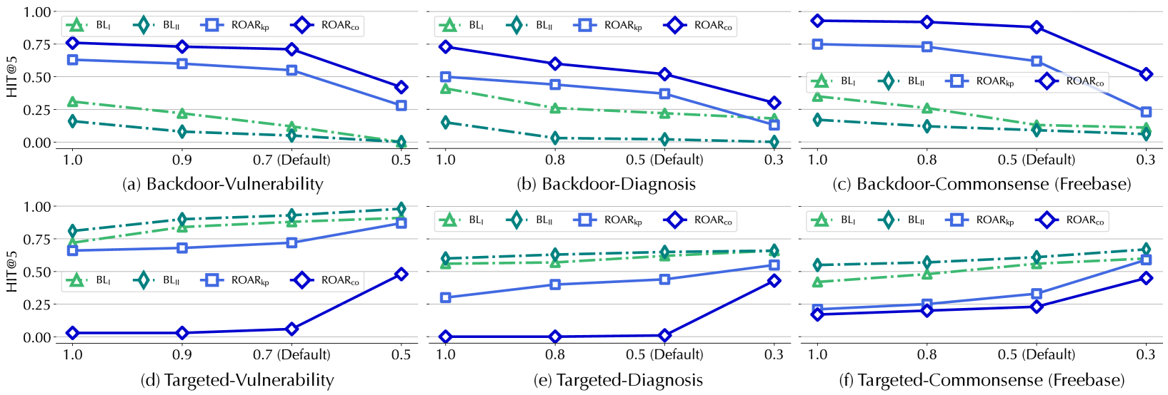
### Key Observations
1. **Inverse Relationship:** The "Backdoor" tasks and "Targeted" tasks exhibit opposite performance behaviors relative to the parameter change. Backdoor performance degrades as the parameter decreases, while Targeted performance improves as the parameter decreases.
2. **Method Sensitivity:** $ROAR_{co}$ (Dark Blue) is consistently the most sensitive method, showing the steepest slopes in both directions (highest peaks in Backdoor, lowest troughs in Targeted).
3. **Baseline Stability:** $BL_I$ and $BL_{II}$ (Green/Teal) are generally more stable across the parameter range compared to the $ROAR$ methods.
4. **Performance Crossover:** In the Targeted scenarios (bottom row), the $ROAR$ methods start with very low performance (near 0.0 in some cases) but improve significantly as the parameter decreases, eventually approaching the performance levels of the $BL$ methods.
### Interpretation
The data suggests that the parameter being adjusted on the X-axis acts as a "sensitivity" or "filtering" control.
* **For Backdoor tasks:** The methods rely on the parameter to maintain high performance. Reducing the parameter likely removes critical information or "backdoor" triggers, causing a sharp decline in HIT@5 scores.
* **For Targeted tasks:** The methods appear to be hindered by the parameter at higher values (1.0). Reducing the parameter likely removes noise or irrelevant data, allowing the models to focus on the target, thereby increasing performance.
* **Peircean Investigative Note:** The stark contrast between the two rows indicates that the underlying mechanism for "Backdoor" detection and "Targeted" detection are fundamentally different in their data requirements. The $ROAR$ methods are highly dynamic, suggesting they are more adaptive to the parameter tuning than the static $BL$ baselines, which maintain a more consistent, albeit sometimes lower, performance profile.
</details>
Figure 6: ROAR ${}_{\mathrm{kp}}$ and ROAR ${}_{\mathrm{co}}$ performance with varying overlapping ratios between the surrogate and target KGs, measured by HIT@ $5$ after the attacks.
Evasiveness. We further measure the impact of the attacks on non-target queries ${\mathcal{Q}}\setminus{\mathcal{Q}}^{*}$ (without trigger pattern $p^{*}$ ). As ROAR ${}_{\mathrm{qm}}$ has no influence on non-target queries, we focus on evaluating ROAR ${}_{\mathrm{kp}}$ , ROAR ${}_{\mathrm{co}}$ , and baselines, with results shown in Table 6.
ROAR has a limited impact on non-target queries. Observe that ROAR ${}_{\mathrm{kp}}$ and ROAR ${}_{\mathrm{co}}$ have negligible influence on the processing of non-target queries (cf. Table 3), with MRR or HIT@ $5$ drop less than 0.05 across all the case. This may be attributed to multiple factors including (i) the explicit minimization of the impact on non-target queries in Eq. 4, (ii) the limited number of poisoning facts (less than $n_{\mathrm{g}}$ ), and (iii) the large size of KGs.
Baselines are less evasive. Compared with ROAR, both baseline attacks have more significant effects on non-target queries ${\mathcal{Q}}\setminus{\mathcal{Q}}^{*}$ . For instance, the MRR of non-target queries drops by 0.12 after the targeted BL ${}_{\mathrm{2}}$ attack against mitigation queries. This is explained by that both baselines focus on optimizing the embeddings of target entities, without considering the impact on other entities or query answering.
### Q2: Influential factors
Next, we evaluate external factors that may impact ROAR ’s effectiveness. Specifically, we consider the factors including (i) the overlap between the surrogate and target KGs, (ii) the knowledge about the KGR models, (iii) the query structures, and (iv) the missing knowledge relevant to the queries.
Knowledge about KG ${\mathcal{G}}$ . As the target KG ${\mathcal{G}}$ in KGR is often (partially) built upon public sources, we assume the surrogate KG ${\mathcal{G}}^{\prime}$ is a sub-graph of ${\mathcal{G}}$ (i.e., we do not require full knowledge of ${\mathcal{G}}$ ). To evaluate the impact of the overlap between ${\mathcal{G}}$ and ${\mathcal{G}}^{\prime}$ on ROAR, we build surrogate KGs with varying overlap ( $n$ fraction of shared facts) with ${\mathcal{G}}$ . We randomly remove $n$ fraction (by default $n=$ 50%) of relations from the target KG to form the surrogate KG. Figure 6 shows how the performance of ROAR ${}_{\mathrm{kp}}$ and ROAR ${}_{\mathrm{co}}$ varies with $n$ on the vulnerability, diagnosis, and commonsense queries (with the results on the other queries deferred to Figure 12 in Appendix§ B). We have the following observations.
ROAR retains effectiveness with limited knowledge. Observe that when $n$ varies in the range of $[0.5,1]$ in the cases of medical decision and commonsense (or $[0.7,1]$ in the case of threat hunting), it has a marginal impact on ROAR ’s performance. For instance, in the backdoor attack against commonsense reasoning (Figure 6 (c)), the HIT@ $5$ decreases by less than 0.15 as $n$ drops from 1 to 0.5. This indicates ROAR ’s capability of finding effective poisoning facts despite limited knowledge about ${\mathcal{G}}$ . However, when $n$ drops below a critical threshold (e.g., 0.3 for medical decision and commonsense, or 0.5 for threat hunting), ROAR ’s performance drops significantly. For instance, the HIT@ $5$ of ROAR ${}_{\mathrm{kp}}$ drops more than 0.39 in the backdoor attack against commonsense reasoning (on Freebase). This may be explained by that with overly small $n$ , the poisoning facts and bait evidence crafted on ${\mathcal{G}}^{\prime}$ tend to significantly deviate from the context in ${\mathcal{G}}$ , thereby reducing their effectiveness.
<details>
<summary>x7.png Details</summary>
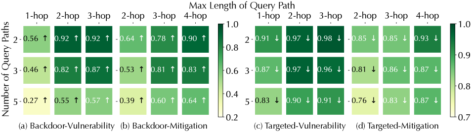
### Visual Description
## Heatmap Matrix: Backdoor and Targeted Vulnerability/Mitigation Analysis
### Overview
This image displays a matrix of four heatmaps, labeled (a) through (d), evaluating the performance or impact of "Backdoor" and "Targeted" scenarios under varying conditions. The vertical axis represents the "Number of Query Paths" (2, 3, 5), and the horizontal axis represents the "Max Length of Query Path" (1-hop, 2-hop, 3-hop). Each cell contains a numerical value and an arrow indicating the direction of the trend (upward or downward).
### Components/Axes
* **Horizontal Axis (Top):** "Max Length of Query Path" (1-hop, 2-hop, 3-hop). This applies to all four sub-charts.
* **Vertical Axis (Left):** "Number of Query Paths" (2, 3, 5). This applies to all four sub-charts.
* **Sub-charts:**
* **(a) Backdoor-Vulnerability:** Left-most heatmap.
* **(b) Backdoor-Mitigation:** Second heatmap from the left.
* **(c) Targeted-Vulnerability:** Third heatmap from the left.
* **(d) Targeted-Mitigation:** Right-most heatmap.
* **Legends:**
* **Left Legend (for a & b):** Scale from 0.2 (light yellow) to 1.0 (dark green).
</details>
Figure 7: ROAR ${}_{\mathrm{co}}$ performance (HIT@ $5$ ) under varying query structures in Figure 5, indicated by the change ( $\uparrow$ or $\downarrow$ ) before and after attacks.
Knowledge about KGR models. Thus far, we assume the surrogate KGR has the same embedding type (e.g., box or vector) and transformation function definition (e.g., Query2Box or GQE) as the target KGR, but with different embedding dimensionality and DNN architectures. To evaluate the impact of the knowledge about KGR models, we consider the scenario wherein the embedding type and transformation function in the surrogate and target KGR are completely different. Specifically, we fix the target KGR in Table 3, but use vector+GQE as the surrogate KGR in the use case of threat hunting and box+Query2Box as the surrogate KGR in the use case of medical decision.
ROAR transfers across KGR models. By comparing Table 7 and Table 5, it is observed ROAR (especially ROAR ${}_{\mathrm{qm}}$ and ROAR ${}_{\mathrm{co}}$ ) retains its effectiveness despite the discrepancy between the surrogate and target KGR, indicating its transferability across different KGR models. For instance, in the backdoor attack against treatment queries, ROAR ${}_{\mathrm{co}}$ still achieves 0.38 MRR increase. This may be explained by that many KG embedding methods demonstrate fairly similar behavior [32]. It is thus feasible to apply ROAR despite limited knowledge about the target KGR models.
| Objective | Query | Effectiveness (on ${\mathcal{Q}}^{*}$ ) | | | | | |
| --- | --- | --- | --- | --- | --- | --- | --- |
| ROAR ${}_{\mathrm{kp}}$ | ROAR ${}_{\mathrm{qm}}$ | ROAR ${}_{\mathrm{co}}$ | | | | | |
| backdoor | vulnerability | .10 $\uparrow$ | .14 $\uparrow$ | .21 $\uparrow$ | .26 $\uparrow$ | .30 $\uparrow$ | .34 $\uparrow$ |
| mitigation | .15 $\uparrow$ | .22 $\uparrow$ | .29 $\uparrow$ | .36 $\uparrow$ | .35 $\uparrow$ | .40 $\uparrow$ | |
| diagnosis | .08 $\uparrow$ | .15 $\uparrow$ | .22 $\uparrow$ | .27 $\uparrow$ | .25 $\uparrow$ | .31 $\uparrow$ | |
| treatment | .33 $\uparrow$ | .50 $\uparrow$ | .36 $\uparrow$ | .52 $\uparrow$ | .38 $\uparrow$ | .59 $\uparrow$ | |
| targeted | vulnerability | .07 $\downarrow$ | .08 $\downarrow$ | .37 $\downarrow$ | .34 $\downarrow$ | .41 $\downarrow$ | .44 $\downarrow$ |
| mitigation | .15 $\downarrow$ | .12 $\downarrow$ | .27 $\downarrow$ | .33 $\downarrow$ | .35 $\downarrow$ | .40 $\downarrow$ | |
| diagnosis | .05 $\downarrow$ | .11 $\downarrow$ | .20 $\downarrow$ | .24 $\downarrow$ | .29 $\downarrow$ | .37 $\downarrow$ | |
| treatment | .01 $\downarrow$ | .03 $\downarrow$ | .08 $\downarrow$ | .11 $\downarrow$ | .15 $\downarrow$ | .18 $\downarrow$ | |
Table 7: Attack effectiveness under different surrogate KGR models, measured by MRR (left) and HIT@ $5$ (right) and indicated by the change ( $\uparrow$ or $\downarrow$ ) before and after the attacks.
Query structures. Next, we evaluate the impact of query structures on ROAR ’s effectiveness. Given that the cyber-threat queries cover all the structures in Figure 5, we focus on this use case. Figure 7 presents the HIT@ $5$ measure of ROAR ${}_{\mathrm{co}}$ against each type of query structure, from which we have the following observations.
Attack performance drops with query path numbers. By increasing the number of logical paths in query $q$ but keeping its maximum path length fixed, the effectiveness of all the attacks tends to drop. This may be explained as follows. Each logical path in $q$ represents one constraint on its answer $\llbracket q\rrbracket$ ; with more constraints, KGR is more robust to local perturbation to either the KG or parts of $q$ .
Attack performance improves with query path length. Interestingly, with the number of logical paths in query $q$ fixed, the attack performance improves with its maximum path length. This may be explained as follows. Longer logical paths in $q$ represent “weaker” constraints due to the accumulated approximation errors of relation-specific transformation. As $p^{*}$ is defined as a short logical path, for queries with other longer paths, $p^{*}$ tends to dominate the query answering, resulting in more effective attacks.
Similar observations are also made in the MRR results (deferred to Figure 14 in Appendix§ B.4).
Missing knowledge. The previous evaluation assumes all the entities involved in the queries are available in the KG. Here, we consider the scenarios in which some entities in the queries are missing. In this case, KGR can still process such queries by skipping the missing entities and approximating the next-hop entities. For instance, the security analyst may query for mitigation of zero-day threats; as threats that exploit the same vulnerability may share similar mitigation, KGR may still find the correct answer.
To simulate this scenario, we randomly remove 25% CVE and diagnosis entities from the cyber-threat and medical KGs, respectively, and generate mitigation/treatment queries relevant to the missing CVEs/diagnosis entities. The other setting follows § 5.1. Table 8 shows the results.
| Obj. | Query | Attack | | | | | | | | | | | |
| --- | --- | --- | --- | --- | --- | --- | --- | --- | --- | --- | --- | --- | --- |
| w/o | BL ${}_{\mathrm{1}}$ | BL ${}_{\mathrm{2}}$ | ROAR ${}_{\mathrm{kp}}$ | ROAR ${}_{\mathrm{qm}}$ | ROAR ${}_{\mathrm{co}}$ | | | | | | | | |
| backdoor | miti. | .00 | .01 | .00 $\uparrow$ | .00 $\uparrow$ | .00 $\uparrow$ | .00 $\uparrow$ | .26 $\uparrow$ | .50 $\uparrow$ | .59 $\uparrow$ | .64 $\uparrow$ | .66 $\uparrow$ | .64 $\uparrow$ |
| treat. | .04 | .08 | .03 $\uparrow$ | .12 $\uparrow$ | .00 $\uparrow$ | .00 $\uparrow$ | .40 $\uparrow$ | .61 $\uparrow$ | .55 $\uparrow$ | .70 $\uparrow$ | .58 $\uparrow$ | .77 $\uparrow$ | |
| targeted | miti. | .57 | .78 | .00 $\downarrow$ | .00 $\downarrow$ | .00 $\downarrow$ | .00 $\downarrow$ | .28 $\downarrow$ | .24 $\downarrow$ | .51 $\downarrow$ | .67 $\downarrow$ | .55 $\downarrow$ | .71 $\downarrow$ |
| treat. | .52 | .70 | .00 $\downarrow$ | .00 $\downarrow$ | .00 $\downarrow$ | .00 $\downarrow$ | .08 $\downarrow$ | .12 $\downarrow$ | .12 $\downarrow$ | .19 $\downarrow$ | .23 $\downarrow$ | .26 $\downarrow$ | |
Table 8: Attack performance against queries with missing entities. The measures in each cell are MRR (left) and HIT@ $5$ (right).
ROAR is effective against missing knowledge. Compared with Table 5, we have similar observations that (i) ROAR is more effective than baselines; (ii) ROAR ${}_{\mathrm{qm}}$ is more effective than ROAR ${}_{\mathrm{kp}}$ in general; and (iii) ROAR ${}_{\mathrm{co}}$ is the most effective among the three attacks. Also, the missing entities (i.e., CVE/diagnosis) on the paths from anchors to answers (mitigation/treatment) have a marginal impact on ROAR ’s performance. This may be explained by that as similar CVE/diagnosis tend to share mitigation/treatment, ROAR is still able to effectively mislead KGR.
<details>
<summary>x8.png Details</summary>
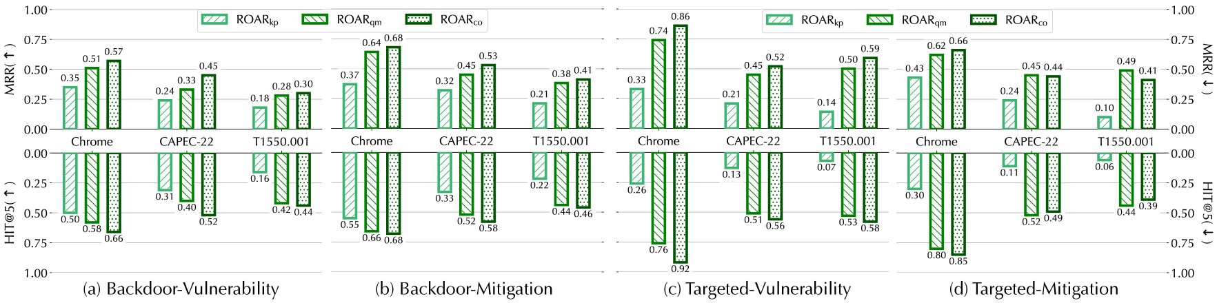
### Visual Description
## Bar Chart: Performance Comparison of ROAR Variants
### Overview
The image presents a composite of four grouped bar charts, labeled (a) through (d), comparing the performance of three variants of a method called "ROAR" (`ROAR_kp`, `ROAR_qm`, `ROAR_co`) across three datasets (Chrome, CAPEC-22, T1550.001). The charts are categorized by task type: Backdoor (Vulnerability/Mitigation) and Targeted (Vulnerability/Mitigation). The metrics used are MRR (Mean Reciprocal Rank) and HIT@5.
### Components/Axes
* **Legend:** Located at the top of the chart (repeated for the left and right halves).
* `ROAR_kp`: Light green, diagonal stripes.
* `ROAR_qm`: Medium green, diagonal stripes.
* `ROAR_co`: Dark green, dotted pattern.
* **X-Axis:** Categorical datasets: Chrome, CAPEC-22, T1550.001.
* **Y-Axis (Top):** MRR (Mean Reciprocal Rank).
* **Y-Axis (Bottom):** HIT@5.
* **Sub-charts:**
* (a) Backdoor-Vulnerability
* (b) Backdoor-Mitigation
* (c) Targeted-Vulnerability
* (d) Targeted-Mitigation
### Detailed Analysis
#### (a) Backdoor-Vulnerability
| Metric | Dataset | ROAR_kp | ROAR_qm | ROAR_co |
| :--- | :--- | :--- | :--- | :--- |
| **MRR** | Chrome | 0.35 | 0.51 | 0.57 |
| | CAPEC-22 | 0.24 | 0.33 | 0.45 |
| | T1550.001 | 0.18 | 0.28 | 0.30 |
| **HIT@5** | Chrome | 0.50 | 0.58 | 0.66 |
| | CAPEC-22 | 0.31 | 0.40 | 0.52 |
| | T1550.001 | 0.16 | 0.42 | 0.44 |
#### (b) Backdoor-Mitigation
| Metric | Dataset | ROAR_kp | ROAR_qm | ROAR_co |
| :--- | :--- | :--- | :--- | :--- |
| **MRR** | Chrome | 0.37 | 0.64 | 0.68 |
| | CAPEC-22 | 0.32 | 0.45 | 0.53 |
| | T1550.001 | 0.21 | 0.38 | 0.41 |
| **HIT@5** | Chrome | 0.55 | 0.66 | 0.68 |
| | CAPEC-22 | 0.22 | 0.52 | 0.58 |
| | T1550.001 | 0.22 | 0.44 | 0.46 |
#### (c) Targeted-Vulnerability
| Metric | Dataset | ROAR_kp | ROAR_qm | ROAR_co |
| :--- | :--- | :--- | :--- | :--- |
| **MRR** | Chrome | 0.33 | 0.74 | 0.86 |
| | CAPEC-22 | 0.21 | 0.45 | 0.52 |
| | T1550.001 | 0.14 | 0.50 | 0.59 |
| **HIT@5** | Chrome | 0.26 | 0.76 | 0.92 |
| | CAPEC-22 | 0.13 | 0.51 | 0.56 |
| | T1550.001 | 0.07 | 0.53 | 0.58 |
#### (d) Targeted-Mitigation
| Metric | Dataset | ROAR_kp | ROAR_qm | ROAR_co |
| :--- | :--- | :--- | :--- | :--- |
| **MRR** | Chrome | 0.43 | 0.62 | 0.66 |
| | CAPEC-22 | 0.24 | 0.45 | 0.44 |
| | T1550.001 | 0.10 | 0.49 | 0.41 |
| **HIT@5** | Chrome | 0.30 | 0.80 | 0.85 |
| | CAPEC-22 | 0.11 | 0.52 | 0.49 |
| | T1550.001 | 0.06 | 0.44 | 0.39 |
### Key Observations
* **Performance Hierarchy:** Across almost all datasets and tasks, `ROAR_co` (dotted) consistently achieves the highest performance, followed by `ROAR_qm`, with `ROAR_kp` (lightest) consistently performing the worst.
* **Dataset Difficulty:** Performance generally trends downward from Chrome to CAPEC-22 to T1550.001, suggesting that the Chrome dataset is the least challenging or most compatible with these methods.
* **Targeted vs. Backdoor:** The Targeted scenarios (c and d) exhibit a wider performance gap between the methods compared to the Backdoor scenarios (a and b), particularly in the Chrome dataset where `ROAR_co` reaches a high of 0.92 in HIT@5.
* **Anomalies:** In (d) Targeted-Mitigation, `ROAR_co` performs slightly worse than `ROAR_qm` for the CAPEC-22 and T1550.001 datasets, breaking the general trend where `ROAR_co` is the top performer.
### Interpretation
The data demonstrates a clear hierarchy of effectiveness among the ROAR variants, with `ROAR_co` being the most robust and effective method. The consistent performance gap between `ROAR_kp` and the other two variants suggests that the modifications introduced in `ROAR_qm` and `ROAR_co` provide substantial improvements in both vulnerability detection and mitigation tasks. The performance degradation across datasets indicates that these models are highly sensitive to the underlying data distribution, with the "Chrome" dataset being significantly more amenable to these methods than the others. The anomaly in the Targeted-Mitigation chart suggests that while `ROAR_co` is generally superior, its advantage is not universal and may be task-dependent.
</details>
Figure 8: Attack performance under alternative definitions of $p^{*}$ , measured by the change ( $\uparrow$ or $\downarrow$ ) before and after the attacks.
<details>
<summary>x9.png Details</summary>
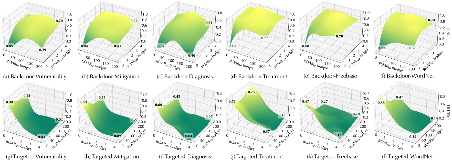
### Visual Description
## 3D Surface Plots: Performance Analysis of Backdoor and Targeted Attacks
### Overview
This image presents a grid of 12 3D surface plots, organized into two rows and six columns. The plots visualize the relationship between two independent variables—$ROAR_{qm}$ budget and $ROAR_{kp}$ budget—and a dependent variable, HIT@5. The top row (a-f) represents "Backdoor" scenarios, while the bottom row (g-l) represents "Targeted" scenarios. The plots demonstrate how the HIT@5 metric changes as the budgets for $ROAR_{qm}$ and $ROAR_{kp}$ are adjusted.
### Components/Axes
* **Grid Layout:**
* **Top Row (a-f):** Backdoor-Vulnerability, Backdoor-Mitigation, Backdoor-Diagnosis, Backdoor-Treatment, Backdoor-Freebase, Backdoor-WordNet.
* **Bottom Row (g-l):** Targeted-Vulnerability, Targeted-Mitigation, Targeted-Diagnosis, Targeted-Treatment, Targeted-Freebase, Targeted-WordNet.
* **Axes (Common to all plots):**
* **X-axis ($ROAR_{qm}$ budget):** Ranges from 0 to 4.
* **Y-axis ($ROAR_{kp}$ budget):** Ranges from 0 to 200.
* **Z-axis (Vertical):** HIT@5, ranging from 0.0 to 1.0 (scales vary slightly by plot).
* **Visual Encoding:**
* **Color:** A gradient from dark green (low values) to yellow (high values).
* **Annotations:** Specific numerical values are provided at the corners of the surfaces to indicate approximate HIT@5 values at those coordinates.
---
### Detailed Analysis
#### Top Row: Backdoor Scenarios
*General Trend:* All Backdoor plots exhibit an upward trend, where HIT@5 values increase as both $ROAR_{qm}$ and $ROAR_{kp}$ budgets increase. The surfaces generally slope from the origin (low) to the far corner (high).
* **(a) Backdoor-Vulnerability:** Starts at ~0.05 (0,0). Rises to ~0.39 at (4,0) and ~0.70 at (4,200).
* **(b) Backdoor-Mitigation:** Starts at ~0.04 (0,0). Rises to ~0.43 at (4,0) and ~0.72 at (4,200).
* **(c) Backdoor-Diagnosis:** Starts at ~0.02 (0,0). Rises to ~0.10 at (4,0) and ~0.51 at (4,200).
* **(d) Backdoor-Treatment:** Starts at ~0.10 (0,0). Rises sharply to ~0.77 at (4,200).
* **(e) Backdoor-Freebase:** Starts at ~0.00 (0,0). Rises sharply to ~0.78 at (4,200).
* **(f) Backdoor-WordNet:** Starts at ~0.00 (0,0). Rises to ~0.57 at (4,0) and ~0.74 at (4,200).
#### Bottom Row: Targeted Scenarios
*General Trend:* All Targeted plots exhibit a downward trend, where HIT@5 values are highest at the origin (0,0) and decrease significantly as budgets increase.
* **(g) Targeted-Vulnerability:** Starts high at ~0.98 (0,0). Drops to ~0.03 at (4,0) and ~0.02 at (4,200). The value at (0,200) is ~0.61.
* **(h) Targeted-Mitigation:** Starts high at ~0.91 (0,0). Drops to ~0.09 at (4,0) and ~0.00 at (4,200). The value at (0,200) is ~0.55.
* **(i) Targeted-Diagnosis:** Starts at ~0.66 (0,0). Drops to ~0.04 at (4,0) and ~0.07 at (4,200). The value at (0,200) is ~0.43.
* **(j) Targeted-Treatment:** Starts at ~0.78 (0,0). Drops to ~0.57 at (4,0) and ~0.45 at (4,200). The value at (0,200) is ~0.75.
* **(k) Targeted-Freebase:** Starts at ~0.67 (0,0). Drops to ~0.13 at (4,0) and ~0.20 at (4,200). The value at (0,200) is ~0.27.
* **(l) Targeted-WordNet:** Starts at ~0.88 (0,0). Drops to ~0.29 at (4,0) and ~0.14 at (4,200). The value at (0,200) is ~0.47.
---
### Key Observations
1. **Inverse Relationship:** The most significant observation is the complete inversion of the surface topography between the Backdoor and Targeted categories. Backdoor performance improves with budget, while Targeted performance degrades with budget.
2. **Sensitivity:** Targeted attacks show high sensitivity to budget increases, with performance often dropping near zero at maximum budget levels (e.g., plots g, h, i).
3. **Consistency:** The behavior is remarkably consistent across the different datasets (Vulnerability, Mitigation, Diagnosis, Treatment, Freebase, WordNet), suggesting that the observed trends are fundamental to the attack types rather than dataset-specific anomalies.
### Interpretation
The data suggests a fundamental divergence in how "Backdoor" and "Targeted" attacks respond to the ROAR budget parameters.
* **Backdoor Attacks:** The positive correlation between budget and HIT@5 suggests that increasing the budget (likely representing the removal or retraining process) actually *increases* the HIT@5 metric. This could imply that the "budget" is not effectively mitigating the backdoor, or that the metric is measuring the success rate of the backdoor itself, which becomes more pronounced or easier to trigger as the model is modified.
* **Targeted Attacks:** The negative correlation suggests that the budget is highly effective at mitigating these attacks. As the budget increases, the HIT@5 (likely representing model accuracy or attack success) drops precipitously.
* **Peircean Investigative Note:** The visual symmetry between the two rows is striking. The "Targeted" plots resemble a "cliff" where performance falls off as resources are applied, whereas the "Backdoor" plots resemble a "ramp" where performance climbs. This implies that the ROAR mechanism acts as a robust defense against Targeted attacks but fails to suppress (or perhaps inadvertently amplifies) Backdoor attacks.
</details>
Figure 9: ROAR ${}_{\mathrm{co}}$ performance with varying budgets (ROAR ${}_{\mathrm{kp}}$ – $n_{\mathrm{g}}$ , ROAR ${}_{\mathrm{qm}}$ – $n_{\mathrm{q}}$ ). The measures are the absolute HIT@ $5$ after the attacks.
### Q3: Alternative settings
Besides the influence of external factors, we also explore ROAR ’s performance under a set of alternative settings.
Alternative $p^{*}$ . Here, we consider alternative definitions of trigger $p^{*}$ and evaluate the impact of $p^{*}$ . Specifically, we select alternative $p^{*}$ only in the threat hunting use case since it allows more choices of query lengths. Besides the default definition (with Google Chrome as the anchor) in § 5.1, we consider two other definitions in Table 9: one with CAPEC-22 http://capec.mitre.org/data/definitions/22.html (attack pattern) as its anchor and its logical path is of length 2 for querying vulnerability and 3 for querying mitigation; the other with T1550.001 https://attack.mitre.org/techniques/T1550/001/ (attack technique) as its anchor is of length 3 for querying vulnerability and 4 for querying mitigation. Figure 8 summarizes ROAR ’s performance under these definitions. We have the following observations.
| anchor of $p^{*}$ | entity | $\mathsf{Google\,\,Chrome}$ | $\mathsf{CAPEC-22}$ | $\mathsf{T1550.001}$ |
| --- | --- | --- | --- | --- |
| category | product | attack pattern | technique | |
| length of $p^{*}$ | vulnerability | 1 hop | 2 hop | 3 hop |
| mitigation | 2 hop | 3 hop | 4 hop | |
Table 9: Alternative definitions of $p^{*}$ , where $\mathsf{Google\,\,Chrome}$ is the anchor of the default $p^{*}$ .
Shorter $p^{*}$ leads to more effective attacks. Comparing Figure 8 and Table 9, we observe that in general, the effectiveness of both ROAR ${}_{\mathrm{kp}}$ and ROAR ${}_{\mathrm{qm}}$ decreases with $p^{*}$ ’s length. This can be explained as follows. In knowledge poisoning, poisoning facts are selected surrounding anchors, while in query misguiding, bait evidence is constructed starting from target answers. Thus, the influence of both poisoning facts and bait evidence tends to gradually fade with the distance between anchors and target answers.
There exists delicate dynamics in ROAR ${}_{\mathrm{co}}$ . Observe that ROAR ${}_{\mathrm{co}}$ shows more complex dynamics with respect to the setting of $p^{*}$ . Compared with ROAR ${}_{\mathrm{kp}}$ , ROAR ${}_{\mathrm{co}}$ seems less sensitive to $p^{*}$ , with MRR $\geq 0.30$ and HIT@ $5$ $\geq 0.44$ under $p^{*}$ with T1550.001 in backdoor attacks; while in targeted attacks, ROAR ${}_{\mathrm{co}}$ performs slightly worse than ROAR ${}_{\mathrm{qm}}$ under the setting of mitigation queries and alternative definitions of $p^{*}$ . This can be explained by the interaction between the two attack vectors within ROAR ${}_{\mathrm{co}}$ : on one hand, the negative impact of $p^{*}$ ’s length on poisoning facts may be compensated by bait evidence; on the other hand, due to their mutual dependency in co-optimization, ineffective poisoning facts also negatively affect the generation of bait evidence.
Attack budgets. We further explore how to properly set the attack budgets in ROAR. We evaluate the attack performance as a function of $n_{\mathrm{g}}$ (number of poisoning facts) and $n_{\mathrm{q}}$ (number of bait evidence), with results summarized in Figure 9.
There exists an “mutual reinforcement” effect. In both backdoor and targeted cases, with one budget fixed, slightly increasing the other significantly improves ROAR ${}_{\mathrm{co}}$ ’s performance. For instance, in backdoor cases, when $n_{\mathrm{g}}=0$ , increasing $n_{\mathrm{q}}$ from 0 to 1 leads to 0.44 improvement in HIT@ $5$ , while increasing $n_{\mathrm{g}}=50$ leads to HIT@ $5$ $=0.58$ . Further, we also observe that ROAR ${}_{\mathrm{co}}$ can easily approach the optimal performance under the setting of $n_{\mathrm{g}}\in[50,100]$ and $n_{\mathrm{q}}\in[1,2]$ , indicating that ROAR ${}_{\mathrm{co}}$ does not require large attack budgets due to the mutual reinforcement effect.
Large budgets may not always be desired. Also, observe that ROAR has degraded performance when $n_{\mathrm{g}}$ is too large (e.g., $n_{\mathrm{g}}=200$ in the backdoor attacks). This may be explained by that a large budget may incur many noisy poisoning facts that negatively interfere with each other. Recall that in knowledge poisoning, ROAR generates poisoning facts in a greedy manner (i.e., top- $n_{\mathrm{g}}$ facts with the highest fitness scores in Algorithm 1) without considering their interactions. Further, due to the gap between the input and latent spaces, the input-space approximation may introduce additional noise in the generated poisoning facts. Thus, the attack performance may not be a monotonic function of $n_{\mathrm{g}}$ . Note that due to the practical constraints of poisoning real-world KGs, $n_{\mathrm{g}}$ tends to be small in practice [56].
We also observe similar trends measured by MRR with results shown in Figure 13 in Appendix§ B.4.
## 6 Discussion
### 6.1 Surrogate KG Construction
We now discuss why building the surrogate KG is feasible. In practice, the target KG is often (partially) built upon some public sources (e.g., Web) and needs to be constantly updated [61]. The adversary may obtain such public information to build the surrogate KG. For instance, to keep up with the constant evolution of cyber threats, threat intelligence KGs often include new threat reports from threat blogs and news [28], which are also accessible to the adversary.
In the evaluation, we simulate the construction of the surrogate KG by randomly removing a fraction of facts from the target KG (50% by default). By controlling the overlapping ratio between the surrogate and target KGs (Figure 6), we show the impact of the knowledge about the target KG on the attack performance.
Zero-knowledge attacks. In the extreme case, the adversary has little knowledge about the target KG and thus cannot build a surrogate KG directly. However, if the query interface of KGR is publicly accessible (as in many cases [8, 2, 12]), the adversary is often able to retrieve subsets of entities and relations from the backend KG and construct a surrogate KG. Specifically, the adversary may use a breadth-first traversal approach to extract a sub-KG: beginning with a small set of entities, at each iteration, the adversary chooses an entity as the anchor and explores all possible relations by querying for entities linked to the anchor through a specific relation; if the query returns a valid response, the adversary adds the entity to the current sub-KG. We consider exploring zero-knowledge attacks as our ongoing work.
### 6.2 Potential countermeasures
We investigate two potential countermeasures tailored to knowledge poisoning and query misguiding.
<details>
<summary>x10.png Details</summary>
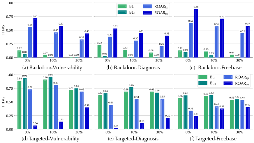
### Visual Description
## Bar Chart: Performance Comparison (HIT@5) across Backdoor and Targeted Scenarios
### Overview
The image presents six grouped bar charts, organized in a 2x3 grid, evaluating the performance of four different methods ($BL_I$, $BL_{II}$, $ROAR_{kp}$, $ROAR_{co}$) across three different perturbation/poisoning levels (0%, 10%, 30%). The charts are categorized into two rows: "Backdoor" scenarios (top row) and "Targeted" scenarios (bottom row). The Y-axis measures "HIT@5," a metric representing the probability of the correct item appearing in the top 5 predictions.
### Components/Axes
* **Y-Axis:** Labeled "HIT@5," ranging from 0.00 to 1.00.
* **X-Axis:** Categorical levels of perturbation/poisoning: 0%, 10%, and 30%.
* **Legend:** Located at the top-center and top-right of the respective rows.
* **$BL_I$**: Light Green
* **$BL_{II}$**: Dark Green/Teal
* **$ROAR_{kp}$**: Light Blue
* **$ROAR_{co}$**: Dark Blue
* **Sub-chart Titles:**
* (a) Backdoor-Vulnerability
* (b) Backdoor-Diagnosis
* (c) Backdoor-Freebase
* (d) Targeted-Vulnerability
* (e) Targeted-Diagnosis
* (f) Targeted-Freebase
---
### Detailed Analysis
#### Row 1: Backdoor Scenarios
*General Trend:* In all three Backdoor charts, the $ROAR$ methods ($ROAR_{kp}$ and $ROAR_{co}$) significantly outperform the $BL$ methods ($BL_I$ and $BL_{II}$). Performance for all methods generally trends downward as the percentage increases from 0% to 30%.
** (a) Backdoor-Vulnerability**
* **0%:** $BL_I$: 0.12, $BL_{II}$: 0.05, $ROAR_{kp}$: 0.55, $ROAR_{co}$: 0.71
* **10%:** $BL_I$: 0.04, $BL_{II}$: 0.00, $ROAR_{kp}$: 0.45, $ROAR_{co}$: 0.57
* **30%:** $BL_I$: 0.00, $BL_{II}$: 0.00, $ROAR_{kp}$: 0.32, $ROAR_{co}$: 0.43
** (b) Backdoor-Diagnosis**
* **0%:** $BL_I$: 0.22, $BL_{II}$: 0.02, $ROAR_{kp}$: 0.37, $ROAR_{co}$: 0.52
* **10%:** $BL_I$: 0.13, $BL_{II}$: 0.00, $ROAR_{kp}$: 0.30, $ROAR_{co}$: 0.44
* **30%:** $BL_I$: 0.08, $BL_{II}$: 0.00, $ROAR_{kp}$: 0.20, $ROAR_{co}$: 0.39
** (c) Backdoor-Freebase**
* **0%:** $BL_I$: 0.12, $BL_{II}$: 0.09, $ROAR_{kp}$: 0.62, $ROAR_{co}$: 0.88
* **10%:** $BL_I$: 0.10, $BL_{II}$: 0.03, $ROAR_{kp}$: 0.56, $ROAR_{co}$: 0.70
* **30%:** $BL_I$: 0.04, $BL_{II}$: 0.00, $ROAR_{kp}$: 0.44, $ROAR_{co}$: 0.57
#### Row 2: Targeted Scenarios
*General Trend:* In the Targeted scenarios, the $BL$ methods ($BL_I$ and $BL_{II}$) significantly outperform the $ROAR$ methods. Performance is generally more stable across the 0%-30% range compared to the Backdoor scenarios.
** (d) Targeted-Vulnerability**
* **0%:** $BL_I$: 0.88, $BL_{II}$: 0.93, $ROAR_{kp}$: 0.72, $ROAR_{co}$: 0.06
* **10%:** $BL_I$: 0.90, $BL_{II}$: 0.95, $ROAR_{kp}$: 0.80, $ROAR_{co}$: 0.13
* **30%:** $BL_I$: 0.71, $BL_{II}$: 0.74, $ROAR_{kp}$: 0.68, $ROAR_{co}$: 0.39
** (e) Targeted-Diagnosis**
* **0%:** $BL_I$: 0.62, $BL_{II}$: 0.65, $ROAR_{kp}$: 0.44, $ROAR_{co}$: 0.01
* **10%:** $BL_I$: 0.68, $BL_{II}$: 0.76, $ROAR_{kp}$: 0.54, $ROAR_{co}$: 0.10
* **30%:** $BL_I$: 0.68, $BL_{II}$: 0.66, $ROAR_{kp}$: 0.55, $ROAR_{co}$: 0.20
** (f) Targeted-Freebase**
* **0%:** $BL_I$: 0.56, $BL_{II}$: 0.61, $ROAR_{kp}$: 0.33, $ROAR_{co}$: 0.23
* **10%:** $BL_I$: 0.60, $BL_{II}$: 0.62, $ROAR_{kp}$: 0.41, $ROAR_{co}$: 0.37
* **30%:** $BL_I$: 0.53, $BL_{II}$: 0.54, $ROAR_{kp}$: 0.52, $ROAR_{co}$: 0.40
---
### Key Observations
* **Method Specialization:** There is a clear dichotomy in performance. $ROAR$ methods are highly effective in Backdoor scenarios but struggle in Targeted scenarios. Conversely, $BL$ methods are highly effective in Targeted scenarios but perform poorly (often near zero) in Backdoor scenarios.
* **Performance Degradation:** In Backdoor scenarios, increasing the perturbation/poisoning percentage consistently degrades performance across all methods.
* **Notable Outliers:**
* $ROAR_{co}$ in Targeted-Diagnosis (0%) shows an extremely low HIT@5 of 0.01.
* $BL_{II}$ in Backdoor-Diagnosis (10% and 30%) and Backdoor-Vulnerability (30%) hits 0.00, indicating a complete failure to identify the target in those conditions.
### Interpretation
The data demonstrates that the choice of method is highly dependent on the specific threat model (Backdoor vs. Targeted). The $ROAR$ family of methods appears to be specifically engineered or suited for detecting or mitigating Backdoor attacks, as evidenced by their dominance in the top row. The $BL$ family appears to be a baseline or alternative approach that is better suited for Targeted scenarios, where it maintains high accuracy while $ROAR$ methods falter. The inverse relationship between the two method families suggests they may be optimizing for different features or utilizing different underlying logic that is mutually exclusive in terms of high performance.
</details>
Figure 10: Attack performance (HIT@ $5$ ) on target queries ${\mathcal{Q}}^{*}$ . The measures are the absolute HIT@ $5$ after the attacks.
Filtering of poisoning facts. Intuitively, as they are artificially injected, poisoning facts tend to be misaligned with their neighboring entities/relations in KGs. Thus, we propose to detect misaligned facts and filter them out to mitigate the influence of poisoning facts. Specifically, we use Eq. 5 to measure the “fitness” of each fact $v\mathrel{\text{\scriptsize$\xrightarrow[]{r}$}}v^{\prime}$ and then remove $m\$ of the facts with the lowest fitness scores.
<details>
<summary>x11.png Details</summary>

### Visual Description
## 3D Surface Plots: HIT@5 Performance Analysis
### Overview
The image presents six 3D surface plots, labeled (a) through (f), illustrating the performance metric "HIT@5" across varying "Attack budget" and "Defense budget" levels. The plots are organized into two distinct categories: "Backdoor" (a, b, c) and "Targeted" (d, e, f). The color gradient in each plot transitions from dark purple (representing lower HIT@5 values) to white (representing higher HIT@5 values).
### Components/Axes
* **X-axis:** "Attack budget" (Scale: 0 to 4).
* **Y-axis:** "Defense budget" (Scale: 0 to 4).
* **Z-axis (Vertical):** "HIT@5" (Scale varies per plot).
* **Labels:**
* (a) Backdoor-Vulnerability
* (b) Backdoor-Diagnosis
* (c) Backdoor-Freebase
* (d) Targeted-Vulnerability
* (e) Targeted-Diagnosis
* (f) Targeted-Freebase
### Detailed Analysis
#### Group 1: Backdoor Scenarios
These plots generally exhibit higher HIT@5 values and show a positive correlation between the Attack budget and performance.
* **(a) Backdoor-Vulnerability**
* **Trend:** The surface slopes upward as the Attack budget increases.
* **Corner Values:**
* Attack 0, Defense 0: ~0.55
* Attack 0, Defense 4: ~0.54
* Attack 4, Defense 0: ~0.80
* Attack 4, Defense 4: ~0.68
* **(b) Backdoor-Diagnosis**
* **Trend:** A distinct peak occurs at high Attack budget and low Defense budget.
* **Corner Values:**
* Attack 0, Defense 0: ~0.37
* Attack 0, Defense 4: ~0.34
* Attack 4, Defense 0: ~0.67
* Attack 4, Defense 4: ~0.38
* **(c) Backdoor-Freebase**
* **Trend:** Similar to (b), with a sharp peak at high Attack budget and low Defense budget.
* **Corner Values:**
* Attack 0, Defense 0: ~0.62
* Attack 0, Defense 4: ~0.51
* Attack 4, Defense 0: ~0.84
* Attack 4, Defense 4: ~0.50
#### Group 2: Targeted Scenarios
These plots show a strong negative correlation with the Defense budget; performance drops significantly as the Defense budget increases.
* **(d) Targeted-Vulnerability**
* **Trend:** High performance at low Defense budget, dropping sharply toward zero as Defense budget increases.
* **Corner Values:**
* Attack 0, Defense 0: ~0.72
* Attack 0, Defense 4: ~0.02
* Attack 4, Defense 0: ~0.70
* Attack 4, Defense 4: ~0.13
* **(e) Targeted-Diagnosis**
* **Trend:** Similar to (d), with performance collapsing as Defense budget increases.
* **Corner Values:**
* Attack 0, Defense 0: ~0.44
* Attack 0, Defense 4: ~0.00
* Attack 4, Defense 0: ~0.40
* Attack 4, Defense 4: ~0.05
* **(f) Targeted-Freebase**
* **Trend:** Performance is moderate at low Defense budget and decreases as Defense budget increases, though the drop is less severe than in (d) and (e).
* **Corner Values:**
* Attack 0, Defense 0: ~0.33
* Attack 0, Defense 4: ~0.14
* Attack 4, Defense 0: ~0.35
* Attack 4, Defense 4: ~0.22
### Key Observations
* **Defense Sensitivity:** The "Targeted" group is highly sensitive to the Defense budget. In all three Targeted plots, increasing the Defense budget from 0 to 4 results in a near-total loss of HIT@5 performance.
* **Attack Resilience:** The "Backdoor" group is more resilient to the Defense budget. While performance fluctuates, it remains significantly higher at a Defense budget of 4 compared to the Targeted group.
* **Performance Ceiling:** The "Backdoor" plots reach higher absolute HIT@5 values (peaking around 0.80–0.84) compared to the "Targeted" plots (peaking around 0.35–0.72).
### Interpretation
The data demonstrates a fundamental difference in the efficacy of attacks between "Backdoor" and "Targeted" scenarios.
1. **Backdoor Attacks:** These appear to be more robust. The "Attack budget" is the primary driver of success; increasing it consistently yields higher HIT@5 scores, and the "Defense budget" has a relatively muted impact on mitigating these attacks.
2. **Targeted Attacks:** These are highly fragile. While they can achieve moderate success when the Defense budget is low, they are easily neutralized by increasing the Defense budget. This suggests that Targeted attacks are significantly easier to defend against than Backdoor attacks.
3. **Task Variance:** The "Freebase" variants (c and f) show slightly different surface curvatures compared to "Vulnerability" and "Diagnosis," indicating that the underlying task or dataset characteristics influence how these attacks interact with defense mechanisms.
</details>
Figure 11: Performance of ROAR ${}_{\mathrm{co}}$ against adversarial training with respect to varying settings of attack $n_{\mathrm{q}}$ and defense $n_{\mathrm{q}}$ (note: in targeted attacks, the attack performance is measured by the HIT@ $5$ drop).
Table 10 measures the KGR performance on non-target queries ${\mathcal{Q}}\setminus{\mathcal{Q}}^{*}$ and the Figure 10 measures attack performance on target queries ${\mathcal{Q}}^{*}$ as functions of $m$ . We have the following observations. (i) The filtering degrades the attack performance. For instance, the HIT@ $5$ of ROAR ${}_{\mathrm{kp}}$ drops by 0.23 in the backdoor attacks against vulnerability queries as $m$ increases from 10 to 30. (ii) Compared with ROAR ${}_{\mathrm{kp}}$ , ROAR ${}_{\mathrm{co}}$ is less sensitive to filtering, which is explained by its use of both knowledge poisoning and query misguiding, with one attack vector compensating for the other. (iii) The filtering also significantly impacts the KGR performance (e.g., its HIT@ $5$ drops by 0.28 under $m$ = 30), suggesting the inherent trade-off between attack resilience and KGR performance.
| Query | Removal ratio ( $m\$ ) | | |
| --- | --- | --- | --- |
| 0% | 10% | 30% | |
| vulnerability | 1.00 | 0.93 | 0.72 |
| diagnosis | 0.87 | 0.84 | 0.67 |
| Freebase | 0.70 | 0.66 | 0.48 |
Table 10: KGR performance (HIT@ $5$ ) on non-target queries ${\mathcal{Q}}\setminus{\mathcal{Q}}^{*}$ .
Training with adversarial queries. We further extend the adversarial training [48] strategy to defend against ROAR ${}_{\mathrm{co}}$ . Specifically, we generate an adversarial version $q^{*}$ for each query $q$ using ROAR ${}_{\mathrm{co}}$ and add $(q^{*},\llbracket q\rrbracket)$ to the training set, where $\llbracket q\rrbracket$ is $q$ ’s ground-truth answer.
We measure the performance of ROAR ${}_{\mathrm{co}}$ under varying settings of $n_{\text{q}}$ used in ROAR ${}_{\mathrm{co}}$ and that used in adversarial training, with results shown in Figure 11. Observe that adversarial training degrades the attack performance against the backdoor attacks (Figure 11 a-c) especially when the defense $n_{\text{q}}$ is larger than the attack $n_{\text{q}}$ . However, the defense is much less effective on the targeted attacks (Figure 11 d-f). This can be explained by the larger attack surface of targeted attacks, which only need to force erroneous reasoning rather than backdoor reasoning. Further, it is inherently ineffective against ROAR ${}_{\mathrm{kp}}$ (when the attack $n_{\text{q}}=0$ in ROAR ${}_{\mathrm{co}}$ ), which does not rely on query misguiding.
We can thus conclude that, to defend against the threats to KGR, it is critical to (i) integrate multiple defense mechanisms and (ii) balance attack resilience and KGR performance.
### 6.3 Limitations
Other threat models and datasets. While ROAR instantiates several attacks in the threat taxonomy in § 3, there are many other possible attacks against KGR. For example, if the adversary has no knowledge about the KGs used in the KGR systems, is it possible to build surrogate KGs from scratch or construct attacks that transfer across different KG domains? Further, the properties of specific KGs (e.g., size, connectivity, and skewness) may potentially bias our findings. We consider exploring other threat models and datasets from other domains as our ongoing research.
Alternative reasoning tasks. We mainly focus on reasoning tasks with one target entity. There exist other reasoning tasks (e.g., path reasoning [67] finds a logical path with given starting and end entities). Intuitively, ROAR is ineffective in such tasks as it requires knowledge about the logical path to perturb intermediate entities on the path. It is worth exploring the vulnerability of such alternative reasoning tasks.
Input-space attacks. While ROAR directly operates on KGs (or queries), there are scenarios in which KGs (or queries) are extracted from real-world inputs. For instance, threat-hunting queries may be generated based on software testing and inspection. In such scenarios, it requires the perturbation to KGs (or queries) to be mapped to valid inputs (e.g., functional programs).
## 7 Related work
Machine learning security. Machine learning models are becoming the targets of various attacks [20]: adversarial evasion crafts adversarial inputs to deceive target models [31, 24]; model poisoning modifies target models’ behavior by polluting training data [39]; backdoor injection creates trojan models such that trigger-embedded inputs are misclassified [46, 43]; functionality stealing constructs replicate models functionally similar to victim models [64]. In response, intensive research is conducted on improving the attack resilience of machine learning models. For instance, existing work explores new training strategies (e.g., adversarial training) [48] and detection mechanisms [29, 42] against adversarial evasion. Yet, such defenses often fail when facing adaptive attacks [17, 45], resulting in a constant arms race.
Graph learning security. Besides general machine learning security, one line of work focuses on the vulnerability of graph learning [41, 65, 69], including adversarial [72, 66, 21], poisoning [73], and backdoor [68] attacks. This work differs from existing attacks against graph learning in several major aspects. (i) Data complexity – while KGs are special forms of graphs, they contain much richer relational information beyond topological structures. (ii) Attack objectives – we focus on attacking the logical reasoning task, whereas most existing attacks aim at the classification [72, 66, 73] or link prediction task [21]. (iii) Roles of graphs/KGs – we target KGR systems with KGs as backend knowledge bases while existing attacks assume graphs as input data to graph learning. (iv) Attack vectors – we generate plausible poisoning facts or bait evidence, which are specifically applicable to KGR; in contrast, previous attacks directly perturb graph structures [66, 21, 73] or node features [72, 68].
Knowledge graph security. The security risks of KGs are gaining growing attention [70, 19, 18, 54, 56]. Yet, most existing work focuses on the task of link prediction (KG completion) and the attack vector of directly modifying KGs. This work departs from prior work in major aspects: (i) we consider reasoning tasks (e.g., processing logical queries), which require vastly different processing from predictive tasks (details in Section § 2); (ii) existing attacks rely on directly modifying the topological structures of KGs (e.g., adding/deleting edges) without accounting for their semantics, while we assume the adversary influences KGR through indirect means with semantic constraints (e.g., injecting probable relations or showing misleading evidence); (iii) we evaluate the attacks in real-world KGR applications; and (iv) we explore potential countermeasures against the proposed attacks.
## 8 Conclusion
This work represents a systematic study of the security risks of knowledge graph reasoning (KGR). We present ROAR, a new class of attacks that instantiate a variety of threats to KGR. We demonstrate the practicality of ROAR in domain-specific and general KGR applications, raising concerns about the current practice of training and operating KGR. We also discuss potential mitigation against ROAR, which sheds light on applying KGR in a more secure manner.
## References
- [1] CVE Details. https://www.cvedetails.com.
- [2] Cyscale Complete cloud visibility & control platform. https://cyscale.com.
- [3] DRKG - Drug Repurposing Knowledge Graph for Covid-19. https://github.com/gnn4dr/DRKG/.
- [4] DrugBank. https://go.drugbank.com.
- [5] Freebase (database). https://en.wikipedia.org/wiki/Freebase_(database).
- [6] Gartner Identifies Top 10 Data and Analytics Technology Trends for 2021. https://www.gartner.com/en/newsroom/press-releases/2021-03-16-gartner-identifies-top-10-data-and-analytics-technologies-trends-for-2021.
- [7] Hetionet. https://het.io.
- [8] Knowledge Graph Search API. https://developers.google.com/knowledge-graph.
- [9] Logrhythm MITRE ATT&CK Module. https://docs.logrhythm.com/docs/kb/threat-detection.
- [10] MITRE ATT&CK. https://attack.mitre.org.
- [11] National Vulnerability Database. https://nvd.nist.gov.
- [12] QIAGEN Clinical Analysis and Interpretation Services. https://digitalinsights.qiagen.com/services-overview/clinical-analysis-and-interpretation-services/.
- [13] The QIAGEN Knowledge Base. https://resources.qiagenbioinformatics.com/flyers-and-brochures/QIAGEN_Knowledge_Base.pdf.
- [14] YAGO: A High-Quality Knowledge Base. https://yago-knowledge.org/.
- [15] Manos Antonakakis, Tim April, Michael Bailey, Matt Bernhard, Elie Bursztein, Jaime Cochran, Zakir Durumeric, J. Alex Halderman, Luca Invernizzi, Michalis Kallitsis, Deepak Kumar, Chaz Lever, Zane Ma, Joshua Mason, Damian Menscher, Chad Seaman, Nick Sullivan, Kurt Thomas, and Yi Zhou. Understanding the Mirai Botnet. In Proceedings of USENIX Security Symposium (SEC), 2017.
- [16] Erik Arakelyan, Daniel Daza, Pasquale Minervini, and Michael Cochez. Complex Query Answering with Neural Link Predictors. In Proceedings of International Conference on Learning Representations (ICLR), 2021.
- [17] Anish Athalye, Nicholas Carlini, and David Wagner. Obfuscated Gradients Give a False Sense of Security: Circumventing Defenses to Adversarial Examples. In Proceedings of IEEE Conference on Machine Learning (ICML), 2018.
- [18] Peru Bhardwaj, John Kelleher, Luca Costabello, and Declan O’Sullivan. Adversarial Attacks on Knowledge Graph Embeddings via Instance Attribution Methods. Proceedings of Conference on Empirical Methods in Natural Language Processing (EMNLP), 2021.
- [19] Peru Bhardwaj, John Kelleher, Luca Costabello, and Declan O’Sullivan. Poisoning Knowledge Graph Embeddings via Relation Inference Patterns. ArXiv e-prints, 2021.
- [20] Battista Biggio and Fabio Roli. Wild Patterns: Ten Years after The Rise of Adversarial Machine Learning. Pattern Recognition, 84:317–331, 2018.
- [21] Aleksandar Bojchevski and Stephan Günnemann. Adversarial Attacks on Node Embeddings via Graph Poisoning. In Proceedings of IEEE Conference on Machine Learning (ICML), 2019.
- [22] Antoine Bordes, Nicolas Usunier, Alberto Garcia-Durán, Jason Weston, and Oksana Yakhnenko. Translating Embeddings for Modeling Multi-Relational Data. In Proceedings of Advances in Neural Information Processing Systems (NeurIPS), 2013.
- [23] Nicholas Carlini, Matthew Jagielski, Christopher A Choquette-Choo, Daniel Paleka, Will Pearce, Hyrum Anderson, Andreas Terzis, Kurt Thomas, and Florian Tramèr. Poisoning Web-Scale Training Datasets is Practical. In ArXiv e-prints, 2023.
- [24] Nicholas Carlini and David A. Wagner. Towards Evaluating the Robustness of Neural Networks. In Proceedings of IEEE Symposium on Security and Privacy (S&P), 2017.
- [25] Antonio Emanuele Cinà, Kathrin Grosse, Ambra Demontis, Sebastiano Vascon, Werner Zellinger, Bernhard A Moser, Alina Oprea, Battista Biggio, Marcello Pelillo, and Fabio Roli. Wild Patterns Reloaded: A Survey of Machine Learning Security against Training Data Poisoning. In ArXiv e-prints, 2022.
- [26] The Conversation. Study Shows AI-generated Fake Cybersecurity Reports Fool Experts. https://theconversation.com/study-shows-ai-generated-fake-reports-fool-experts-160909.
- [27] Nilesh Dalvi and Dan Suciu. Efficient Query Evaluation on Probabilistic Databases. The VLDB Journal, 2007.
- [28] Peng Gao, Fei Shao, Xiaoyuan Liu, Xusheng Xiao, Zheng Qin, Fengyuan Xu, Prateek Mittal, Sanjeev R Kulkarni, and Dawn Song. Enabling Efficient Cyber Threat Hunting with Cyber Threat Intelligence. In Proceedings of International Conference on Data Engineering (ICDE), 2021.
- [29] Timon Gehr, Matthew Mirman, Dana Drachsler-Cohen, Petar Tsankov, Swarat Chaudhuri, and Martin Vechev. AI2: Safety and Robustness Certification of Neural Networks with Abstract Interpretation. In Proceedings of IEEE Symposium on Security and Privacy (S&P), 2018.
- [30] Fan Gong, Meng Wang, Haofen Wang, Sen Wang, and Mengyue Liu. SMR: Medical Knowledge Graph Embedding for Safe Medicine Recommendation. Big Data Research, 2021.
- [31] Ian Goodfellow, Jonathon Shlens, and Christian Szegedy. Explaining and Harnessing Adversarial Examples. In Proceedings of International Conference on Learning Representations (ICLR), 2015.
- [32] Kelvin Guu, John Miller, and Percy Liang. Traversing Knowledge Graphs in Vector Space. In Proceedings of Conference on Empirical Methods in Natural Language Processing (EMNLP), 2015.
- [33] William L. Hamilton, Payal Bajaj, Marinka Zitnik, Dan Jurafsky, and Jure Leskovec. Embedding Logical Queries on Knowledge Graphs. In Proceedings of Advances in Neural Information Processing Systems (NeurIPS), 2018.
- [34] Wajih Ul Hassan, Adam Bates, and Daniel Marino. Tactical Provenance Analysis for Endpoint Detection and Response Systems. In Proceedings of IEEE Symposium on Security and Privacy (S&P), 2020.
- [35] Shizhu He, Kang Liu, Guoliang Ji, and Jun Zhao. Learning to Represent Knowledge Graphs with Gaussian Embedding. In Proceeddings of ACM Conference on Information and Knowledge Management (CIKM), 2015.
- [36] Erik Hemberg, Jonathan Kelly, Michal Shlapentokh-Rothman, Bryn Reinstadler, Katherine Xu, Nick Rutar, and Una-May O’Reilly. Linking Threat Tactics, Techniques, and Patterns with Defensive Weaknesses, Vulnerabilities and Affected Platform Configurations for Cyber Hunting. ArXiv e-prints, 2020.
- [37] Keman Huang, Michael Siegel, and Stuart Madnick. Systematically Understanding the Cyber Attack Business: A Survey. ACM Computing Surveys (CSUR), 2018.
- [38] Haozhe Ji, Pei Ke, Shaohan Huang, Furu Wei, Xiaoyan Zhu, and Minlie Huang. Language Generation with Multi-hop Reasoning on Commonsense Knowledge Graph. In Proceedings of Conference on Empirical Methods in Natural Language Processing (EMNLP), 2020.
- [39] Yujie Ji, Xinyang Zhang, Shouling Ji, Xiapu Luo, and Ting Wang. Model-Reuse Attacks on Deep Learning Systems. In Proceedings of ACM Conference on Computer and Communications (CCS), 2018.
- [40] Peter E Kaloroumakis and Michael J Smith. Toward a Knowledge Graph of Cybersecurity Countermeasures. The MITRE Corporation, 2021.
- [41] Thomas N. Kipf and Max Welling. Semi-Supervised Classification with Graph Convolutional Networks. In Proceedings of International Conference on Learning Representations (ICLR), 2017.
- [42] Changjiang Li, Shouling Ji, Haiqin Weng, Bo Li, Jie Shi, Raheem Beyah, Shanqing Guo, Zonghui Wang, and Ting Wang. Towards Certifying the Asymmetric Robustness for Neural Networks: Quantification and Applications. IEEE Transactions on Dependable and Secure Computing, 19(6):3987–4001, 2022.
- [43] Changjiang Li, Ren Pang, Zhaohan Xi, Tianyu Du, Shouling Ji, Yuan Yao, and Ting Wang. Demystifying Self-supervised Trojan Attacks. 2022.
- [44] Bill Yuchen Lin, Xinyue Chen, Jamin Chen, and Xiang Ren. Kagnet: Knowledge-aware Graph Networks for Commonsense Reasoning. In Proceedings of Conference on Empirical Methods in Natural Language Processing (EMNLP), 2019.
- [45] Xiang Ling, Shouling Ji, Jiaxu Zou, Jiannan Wang, Chunming Wu, Bo Li, and Ting Wang. DEEPSEC: A Uniform Platform for Security Analysis of Deep Learning Model. In Proceedings of IEEE Symposium on Security and Privacy (S&P), 2019.
- [46] Yingqi Liu, Shiqing Ma, Yousra Aafer, Wen-Chuan Lee, Juan Zhai, Weihang Wang, and Xiangyu Zhang. Trojaning Attack on Neural Networks. In Proceedings of Network and Distributed System Security Symposium (NDSS), 2018.
- [47] Logrhythm. Using MITRE ATT&CK in Threat Hunting and Detection. https://logrhythm.com/uws-using-mitre-attack-in-threat-hunting-and-detection-white-paper/.
- [48] Aleksander Madry, Aleksandar Makelov, Ludwig Schmidt, Dimitris Tsipras, and Adrian Vladu. Towards Deep Learning Models Resistant to Adversarial Attacks. In Proceedings of International Conference on Learning Representations (ICLR), 2018.
- [49] Fabrizio Mafessoni, Rashmi B Prasad, Leif Groop, Ola Hansson, and Kay Prüfer. Turning Vice into Virtue: Using Batch-effects to Detect Errors in Large Genomic Data Sets. Genome biology and evolution, 10(10):2697–2708, 2018.
- [50] Sadegh M Milajerdi, Rigel Gjomemo, Birhanu Eshete, Ramachandran Sekar, and VN Venkatakrishnan. Holmes: Real-time APT Detection through Correlation of Suspicious Information Flows. In Proceedings of IEEE Symposium on Security and Privacy (S&P), 2019.
- [51] Shaswata Mitra, Aritran Piplai, Sudip Mittal, and Anupam Joshi. Combating Fake Cyber Threat Intelligence Using Provenance in Cybersecurity Knowledge Graphs. In 2021 IEEE International Conference on Big Data (Big Data). IEEE, 2021.
- [52] Sudip Mittal, Anupam Joshi, and Tim Finin. Cyber-all-intel: An AI for Security Related Threat Intelligence. In ArXiv e-prints, 2019.
- [53] Bethany Percha and Russ B Altman. A Global Network of Biomedical Relationships Derived from Text. Bioinformatics, 2018.
- [54] Pouya Pezeshkpour, Yifan Tian, and Sameer Singh. Investigating Robustness and Interpretability of Link Prediction via Adversarial Modifications. ArXiv e-prints, 2019.
- [55] Radware. “BrickerBot” Results In Permanent Denial-of-Service. https://www.radware.com/security/ddos-threats-attacks/brickerbot-pdos-permanent-denial-of-service/.
- [56] Mrigank Raman, Aaron Chan, Siddhant Agarwal, Peifeng Wang, Hansen Wang, Sungchul Kim, Ryan Rossi, Handong Zhao, Nedim Lipka, and Xiang Ren. Learning to Deceive Knowledge Graph Augmented Models via Targeted Perturbation. Proceedings of International Conference on Learning Representations (ICLR), 2021.
- [57] Priyanka Ranade, Aritran Piplai, Sudip Mittal, Anupam Joshi, and Tim Finin. Generating Fake Cyber Threat Intelligence Using Transformer-based Models. In 2021 International Joint Conference on Neural Networks (IJCNN). IEEE, 2021.
- [58] Hongyu Ren, Hanjun Dai, Bo Dai, Xinyun Chen, Michihiro Yasunaga, Haitian Sun, Dale Schuurmans, Jure Leskovec, and Denny Zhou. LEGO: Latent Execution-Guided Reasoning for Multi-Hop Question Answering on Knowledge Graphs. In Proceedings of IEEE Conference on Machine Learning (ICML), 2021.
- [59] Hongyu Ren, Weihua Hu, and Jure Leskovec. Query2box: Reasoning over Knowledge Graphs in Vector Space using Box Embeddings. In Proceedings of International Conference on Learning Representations (ICLR), 2020.
- [60] Hongyu Ren and Jure Leskovec. Beta Embeddings for Multi-Hop Logical Reasoning in Knowledge Graphs. In Proceedings of Advances in Neural Information Processing Systems (NeurIPS), 2020.
- [61] Anderson Rossanez, Julio Cesar dos Reis, Ricardo da Silva Torres, and Hèléne de Ribaupierre. KGen: A Knowledge Graph Generator from Biomedical Scientific Literature. BMC Medical Informatics and Decision Making, 20(4):314, 2020.
- [62] Alberto Santos, Ana R Colaço, Annelaura B Nielsen, Lili Niu, Maximilian Strauss, Philipp E Geyer, Fabian Coscia, Nicolai J Wewer Albrechtsen, Filip Mundt, Lars Juhl Jensen, et al. A Knowledge Graph to Interpret Clinical Proteomics Data. Nature Biotechnology, 2022.
- [63] Komal Teru, Etienne Denis, and Will Hamilton. Inductive Relation Prediction by Subgraph Reasoning. In Proceedings of IEEE Conference on Machine Learning (ICML), 2020.
- [64] Florian Tramèr, Fan Zhang, Ari Juels, Michael K. Reiter, and Thomas Ristenpart. Stealing Machine Learning Models via Prediction APIs. In Proceedings of USENIX Security Symposium (SEC), 2016.
- [65] Petar Veličković, Guillem Cucurull, Arantxa Casanova, Adriana Romero, Pietro Liò, and Yoshua Bengio. Graph Attention Networks. In Proceedings of International Conference on Learning Representations (ICLR), 2018.
- [66] Binghui Wang and Neil Zhenqiang Gong. Attacking Graph-based Classification via Manipulating the Graph Structure. In Proceedings of ACM SAC Conference on Computer and Communications (CCS), 2019.
- [67] Xiang Wang, Dingxian Wang, Canran Xu, Xiangnan He, Yixin Cao, and Tat-Seng Chua. Explainable Reasoning over Knowledge Graphs for Recommendation. In Proceedings of AAAI Conference on Artificial Intelligence (AAAI), 2019.
- [68] Zhaohan Xi, Ren Pang, Shouling Ji, and Ting Wang. Graph backdoor. In Proceedings of USENIX Security Symposium (SEC), 2021.
- [69] Kaidi Xu, Hongge Chen, Sijia Liu, Pin-Yu Chen, Tsui-Wei Weng, Mingyi Hong, and Xue Lin. Topology Attack and Defense for Graph Neural Networks: An Optimization Perspective. In Proceedings of International Joint Conference on Artificial Intelligence (IJCAI), 2019.
- [70] Hengtong Zhang, Tianhang Zheng, Jing Gao, Chenglin Miao, Lu Su, Yaliang Li, and Kui Ren. Data Poisoning Attack against Knowledge Graph Embedding. In Proceedings of International Joint Conference on Artificial Intelligence (IJCAI), 2019.
- [71] Yongjun Zhu, Chao Che, Bo Jin, Ningrui Zhang, Chang Su, and Fei Wang. Knowledge-driven drug repurposing using a comprehensive drug knowledge graph. Health Informatics Journal, 2020.
- [72] Daniel Zügner, Amir Akbarnejad, and Stephan Günnemann. Adversarial Attacks on Neural Networks for Graph Data. In Proceedings of ACM International Conference on Knowledge Discovery and Data Mining (KDD), 2018.
- [73] Daniel Zügner and Stephan Günnemann. Adversarial Attacks on Graph Neural Networks via Meta Learning. In Proceedings of International Conference on Learning Representations (ICLR), 2019.
## Appendix A Notations
Table 11 summarizes notations and definitions used through this paper.
| Notation | Definition |
| --- | --- |
| Knowledge graph related | |
| ${\mathcal{G}}$ | a knowledge graph (KG) |
| ${\mathcal{G}}^{\prime}$ | a surrogate knowledge graph |
| $\langle v,r,v^{\prime}\rangle$ | a KG fact from entity $v$ to $v^{\prime}$ with relation $r$ |
| ${\mathcal{N}},{\mathcal{E}},{\mathcal{R}}$ | entity, edge, and relation set of ${\mathcal{G}}$ |
| ${\mathcal{G}}^{+}$ | the poisoning facts on KG |
| Query related | |
| $q$ | a single query |
| $\llbracket q\rrbracket$ | $q$ ’s ground-truth answer(s) |
| $a^{*}$ | the targeted answer |
| ${\mathcal{A}}_{q}$ | anchor entities of query $q$ |
| $p^{*}$ | the trigger pattern |
| ${\mathcal{Q}}$ | a query set |
| ${\mathcal{Q}}^{*}$ | a query set of interest (each $q\in{\mathcal{Q}}^{*}$ contains $p^{*}$ ) |
| $q^{+}$ | the generated bait evidence |
| $q^{*}$ | the infected query, i.e. $q^{*}=q\wedge q^{+}$ |
| Model or embedding related | |
| $\phi$ | a general symbol to represent embeddings |
| $\phi_{{\mathcal{G}}}$ | embeddings of all KG entities |
| $\phi_{v}$ | entity $v$ ’s embedding |
| $\phi_{q}$ | $q$ ’s embedding |
| $\phi_{{\mathcal{G}}^{+}}$ | embeddings we aim to perturb |
| $\phi_{q^{+}}$ | $q^{+}$ ’s embedding |
| $\psi$ | the logical operator(s) |
| $\psi_{r}$ | the relation ( $r$ )-specific operator |
| $\psi_{\wedge}$ | the intersection operator |
| Other parameters | |
| $n_{\mathrm{g}}$ | knowledge poisoning budget |
| $n_{\mathrm{q}}$ | query misguiding budget |
Table 11: Notations, definitions, and categories.
## Appendix B Additonal details
### B.1 KGR training
Following [59], we train KGR in an end-to-end manner. Specifically, given KG ${\mathcal{G}}$ and the randomly initialized embedding function $\phi$ and transformation function $\psi$ , we sample a set of query-answer pairs $(q,\llbracket q\rrbracket)$ from ${\mathcal{G}}$ to form the training set and optimize $\phi$ and $\psi$ to minimize the loss function, which is defined as the embedding distance between the prediction regarding each $q$ and $\llbracket q\rrbracket$ .
### B.2 Parameter setting
Table 12 lists the default parameter setting used in § 5.
| Type | Parameter | Setting |
| --- | --- | --- |
| KGR | $\phi$ dimension | 300 |
| $\phi$ dimension (surrogate) | 200 | |
| $\psi_{r}$ architecture | 4-layer FC | |
| $\psi_{\wedge}$ architecture | 4-layer FC | |
| $\psi_{r}$ architecture (surrogate) | 2-layer FC | |
| $\psi_{\wedge}$ architecture (surrogate) | 2-layer FC | |
| Training | Learning rate | 0.001 |
| Batch size | 512 | |
| KGR epochs | 50000 | |
| ROAR optimization epochs | 10000 | |
| Optimizer (KGR and ROAR) | Adam | |
| Other | $n_{\mathrm{g}}$ | 100 |
| $n_{\mathrm{q}}$ | 2 | |
Table 12: Default parameter setting.
### B.3 Extension to targeted attacks
It is straightforward to extend ROAR to targeted attacks, in which the adversary aims to simply force KGR to make erroneous reasoning over the target queries ${\mathcal{Q}}^{*}$ . To this end, we may maximize the distance between the embedding $\phi_{q}$ of each query $q\in{\mathcal{Q}}^{*}$ and its ground-truth answer $\llbracket q\rrbracket$ .
Specifically, in knowledge poisoning, we re-define the loss function in Eq. 4 as:
$$
\begin{split}\ell_{\text{kp}}(\phi_{{\mathcal{G}}^{+}})=\,&\mathbb{E}_{q\in{
\mathcal{Q}}\setminus{\mathcal{Q}}^{*}}\Delta(\psi(q;\phi_{{\mathcal{G}}^{+}})
,\phi_{\llbracket q\rrbracket})-\\
&\lambda\mathbb{E}_{q\in{\mathcal{Q}}^{*}}\Delta(\psi(q;\phi_{{\mathcal{G}}^{+
}}),\phi_{\llbracket q\rrbracket})\end{split} \tag{8}
$$
In query misguiding, we re-define Eq. 6 as:
$$
\ell_{\text{qm}}(\phi_{q^{+}})=-\Delta(\psi_{\wedge}(\phi_{q},\phi_{q^{+}}),\,
\phi_{\llbracket q\rrbracket}) \tag{9}
$$
The remaining steps are the same as the backdoor attacks.
### B.4 Additional results
This part shows the additional experiments as the complement of section§ 5.
Additional query tasks under variant surrogate KGs. Figure 12 presents the attack performance on other query tasks that are not included in Figure 6. We can observe a similar trend as concluded in§ 5.
MRR results. Figure 14 shows the MRR of ROAR ${}_{\mathrm{co}}$ with respect to different query structures, with observations similar to Figure 7. Figure 13 shows the MRR of ROAR with respect to attack budgets ( $n_{\mathrm{g}}$ , $n_{\mathrm{q}}$ ), with observations similar to Figure 9.
<details>
<summary>x12.png Details</summary>
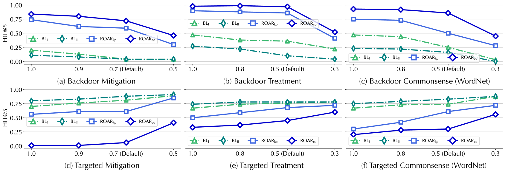
### Visual Description
## Line Charts: Performance Comparison of Mitigation/Treatment Methods
### Overview
The image presents a 2x3 grid of six line charts, labeled (a) through (f). These charts compare the performance (measured by "HIT@5" on the Y-axis) of four distinct methods ($BL_I$, $BL_{II}$, $ROAR_{kp}$, and $ROAR_{co}$) across different experimental settings. The charts are divided into two rows: the top row (a, b, c) relates to "Backdoor" scenarios, and the bottom row (d, e, f) relates to "Targeted" scenarios.
### Components/Axes
* **Y-Axis:** Labeled "HIT@5" for all charts, with a scale ranging from 0.00 to 1.00.
* **X-Axis:** Represents a parameter value (likely a retention or pruning ratio). The values vary by chart:
* (a) and (d): 1.0, 0.9, 0.7 (Default), 0.5.
* (b), (c), (e), and (f): 1.0, 0.8, 0.5 (Default), 0.3.
* **Legend:** Positioned within each chart (typically bottom-left or center-left). The legend is consistent across all six charts:
* **$BL_I$**: Light green line, triangle marker, dashed line style.
* **$BL_{II}$**: Dark teal/green line, diamond marker, dash-dot line style.
* **$ROAR_{kp}$**: Light blue line, square marker, solid line style.
* **$ROAR_{co}$**: Dark blue line, diamond marker, solid line style.
---
### Detailed Analysis
#### Row 1: Backdoor Scenarios
In these charts, all performance metrics trend **downward** as the X-axis value decreases.
* **(a) Backdoor-Mitigation:**
* $ROAR_{co}$ (Dark Blue): Starts at ~0.85, drops to ~0.45.
* $ROAR_{kp}$ (Light Blue): Starts at ~0.75, drops to ~0.30.
* $BL_I$ (Light Green): Starts at ~0.20, drops to ~0.05.
* $BL_{II}$ (Dark Teal): Starts at ~0.12, drops to ~0.05.
* **(b) Backdoor-Treatment:**
* $ROAR_{co}$: Starts at ~0.98, drops to ~0.50.
* $ROAR_{kp}$: Starts at ~0.90, drops to ~0.40.
* $BL_I$: Starts at ~0.45, drops to ~0.20.
* $BL_{II}$: Starts at ~0.25, drops to ~0.05.
* **(c) Backdoor-Commonsense (WordNet):**
* $ROAR_{co}$: Starts at ~0.95, drops to ~0.45.
* $ROAR_{kp}$: Starts at ~0.75, drops to ~0.30.
* $BL_I$: Starts at ~0.45, drops to ~0.05.
* $BL_{II}$: Starts at ~0.20, drops to ~0.05.
#### Row 2: Targeted Scenarios
In these charts, all performance metrics trend **upward** as the X-axis value decreases.
* **(d) Targeted-Mitigation:**
* $BL_{II}$: Starts at ~0.80, rises to ~0.90.
* $BL_I$: Starts at ~0.70, rises to ~0.85.
* $ROAR_{kp}$: Starts at ~0.55, rises to ~0.85.
* $ROAR_{co}$: Starts at ~0.00, rises to ~0.40.
* **(e) Targeted-Treatment:**
* $BL_{II}$: Starts at ~0.75, rises to ~0.80.
* $BL_I$: Starts at ~0.65, rises to ~0.75.
* $ROAR_{kp}$: Starts at ~0.50, rises to ~0.70.
* $ROAR_{co}$: Starts at ~0.35, rises to ~0.60.
* **(f) Targeted-Commonsense (WordNet):**
* $BL_{II}$: Starts at ~0.75, rises to ~0.90.
* $BL_I$: Starts at ~0.70, rises to ~0.85.
* $ROAR_{kp}$: Starts at ~0.30, rises to ~0.70.
* $ROAR_{co}$: Starts at ~0.20, rises to ~0.55.
---
### Key Observations
1. **Inverse Trends:** The "Backdoor" charts show a positive correlation between the X-axis value and HIT@5 (higher retention = higher HIT@5). The "Targeted" charts show a negative correlation (lower retention = higher HIT@5).
2. **Method Dominance:**
* In **Backdoor** scenarios, the $ROAR$ methods ($ROAR_{co}$ and $ROAR_{kp}$) significantly outperform the baselines ($BL_I$ and $BL_{II}$).
* In **Targeted** scenarios, the baselines ($BL_I$ and $BL_{II}$) generally outperform the $ROAR$ methods, although the gap narrows as the X-axis value decreases.
### Interpretation
The data suggests that the X-axis represents a feature retention ratio (e.g., keeping the top X% of features).
* **Backdoor Scenarios:** The goal is likely to remove backdoor triggers. High retention (1.0) keeps the triggers intact, resulting in high HIT@5 (the model is "fooled"). As retention decreases, the triggers are removed, causing the HIT@5 to drop. The $ROAR$ methods are highly effective at this, as evidenced by their higher initial HIT@5 and steeper decline compared to baselines.
* **Targeted Scenarios:** The goal is likely to improve model accuracy on a specific task. Here, lower retention (0.3) appears to remove noise or irrelevant features, allowing the model to focus on the target, thereby increasing HIT@5. The baselines are more robust in this scenario, while the $ROAR$ methods struggle more at high retention levels but improve as more features are pruned.
</details>
Figure 12: ROAR ${}_{\mathrm{kp}}$ and ROAR ${}_{\mathrm{co}}$ performance with varying overlapping ratios between the surrogate and target KGs, measured by HIT@ $5$ after the attacks on other query tasks besides Figure 6.
<details>
<summary>x13.png Details</summary>
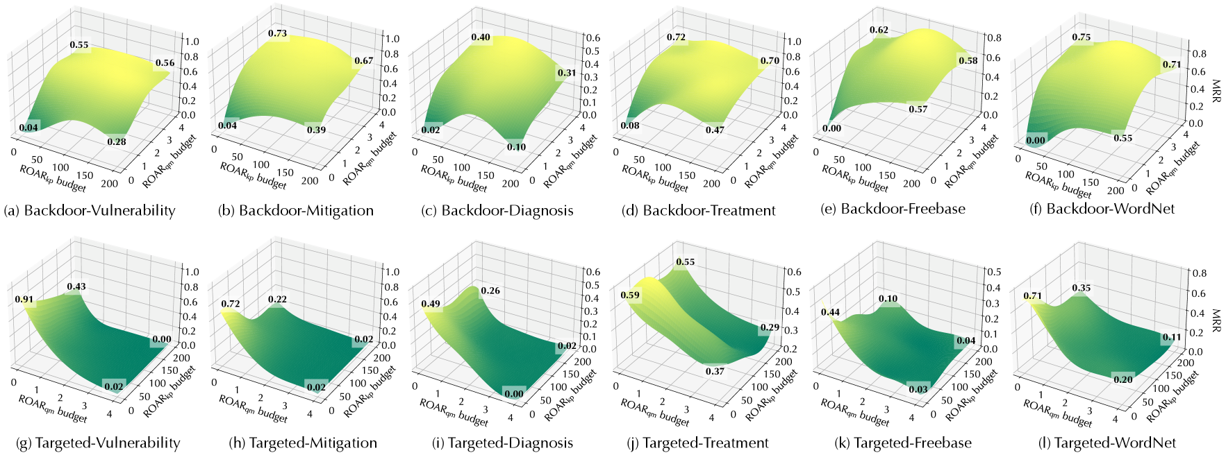
### Visual Description
## 3D Surface Plots: ROAR Budget Analysis (Backdoor vs. Targeted)
### Overview
This image presents a grid of 12 3D surface plots organized into two rows. The top row (a-f) represents "Backdoor" tasks, and the bottom row (g-l) represents "Targeted" tasks. Each plot visualizes the relationship between two budget variables (`ROAR_kp budget` and `ROAR_qm budget`) and a performance metric, `MRR` (Mean Reciprocal Rank), represented on the vertical Z-axis. The color gradient transitions from dark green (low MRR) to bright yellow (high MRR).
### Components/Axes
* **Top Row (a-f):**
* **X-axis:** `ROAR_kp budget` (Scale: 0, 50, 100, 150, 200).
* **Y-axis:** `ROAR_qm budget` (Scale: 0, 1, 2, 3, 4).
* **Z-axis:** `MRR` (Scale: 0.0 to 1.0, varies slightly by plot).
* **Bottom Row (g-l):**
* **X-axis:** `ROAR_qm budget` (Scale: 0, 1, 2, 3, 4).
* **Y-axis:** `ROAR_kp budget` (Scale: 0, 50, 100, 150, 200).
* **Z-axis:** `MRR` (Scale: 0.0 to 1.0, varies slightly by plot).
* **Color Mapping:** Yellow indicates higher MRR values; dark green indicates lower MRR values.
---
### Detailed Analysis
#### Row 1: Backdoor Tasks
*Note: In this row, MRR generally increases as `ROAR_qm budget` increases (moving toward the back of the plot).*
* **(a) Backdoor-Vulnerability:** Peaks at 0.55 (back-left) and 0.56 (back-right). Lows at 0.04 (front-left) and 0.28 (front-right).
* **(b) Backdoor-Mitigation:** Peaks at 0.73 (back-left) and 0.67 (back-right). Lows at 0.04 (front-left) and 0.39 (front-right).
* **(c) Backdoor-Diagnosis:** Peaks at 0.40 (back-left) and 0.31 (back-right). Lows at 0.02 (front-left) and 0.10 (front-right).
* **(d) Backdoor-Treatment:** Peaks at 0.72 (back-left) and 0.70 (back-right). Lows at 0.08 (front-left) and 0.47 (front-right).
* **(e) Backdoor-Freebase:** Peaks at 0.62 (back-left) and 0.58 (back-right). Lows at 0.00 (front-left) and 0.57 (front-right).
* **(f) Backdoor-WordNet:** Peaks at 0.75 (back-left) and 0.71 (back-right). Lows at 0.00 (front-left) and 0.55 (front-right).
#### Row 2: Targeted Tasks
*Note: The axes are swapped compared to the top row. MRR generally decreases as `ROAR_qm budget` increases (moving toward the right of the plot).*
* **(g) Targeted-Vulnerability:** Peaks at 0.91 (front-left) and 0.43 (back-left). Lows at 0.02 (front-right) and 0.00 (back-right).
* **(h) Targeted-Mitigation:** Peaks at 0.72 (front-left) and 0.22 (back-left). Lows at 0.02 (front-right) and 0.02 (back-right).
* **(i) Targeted-Diagnosis:** Peaks at 0.49 (front-left) and 0.26 (back-left). Lows at 0.00 (front-right) and 0.02 (back-right).
* **(j) Targeted-Treatment:** Peaks at 0.59 (front-left) and 0.55 (back-left). Lows at 0.37 (front-right) and 0.29 (back-right).
* **(k) Targeted-Freebase:** Peaks at 0.44 (front-left) and 0.10 (back-left). Lows at 0.03 (front-right) and 0.04 (back-right).
* **(l) Targeted-WordNet:** Peaks at 0.71 (front-left) and 0.35 (back-left). Lows at 0.20 (front-right) and 0.11 (back-right).
---
### Key Observations
1. **Axis Inversion:** The most significant observation is the structural difference between the two rows. In the "Backdoor" row, the `ROAR_qm` budget is on the Y-axis (depth), whereas in the "Targeted" row, the `ROAR_qm` budget is on the X-axis (width).
2. **Inverse Performance Trends:**
* **Backdoor:** Performance (MRR) is positively correlated with the `ROAR_qm` budget; the surface slopes upward toward the back of the plots.
* **Targeted:** Performance (MRR) is negatively correlated with the `ROAR_qm` budget; the surface slopes downward toward the right of the plots.
3. **Budget Sensitivity:** The `ROAR_qm` budget appears to be the primary driver of performance variance in both categories, while the `ROAR_kp` budget has a more subtle, secondary effect on the MRR.
### Interpretation
The data demonstrates a fundamental divergence in how the `ROAR_qm` budget influences model performance depending on the task type.
For **Backdoor** tasks, the system benefits from higher `ROAR_qm` budgets, suggesting that these tasks require more "qm" resources to achieve higher accuracy (MRR). Conversely, for **Targeted** tasks, increasing the `ROAR_qm` budget is detrimental to performance, causing a sharp decline in MRR. This suggests that the `ROAR_qm` budget might be introducing noise or over-fitting in the Targeted tasks, or that the resource allocation strategy is fundamentally incompatible with the Targeted task objective. The consistency of this pattern across all sub-tasks (Vulnerability, Mitigation, Diagnosis, Treatment, Freebase, WordNet) indicates this is a systemic behavior of the model or the evaluation framework being tested.
</details>
Figure 13: ROAR ${}_{\mathrm{co}}$ performance with varying budgets (ROAR ${}_{\mathrm{kp}}$ – $n_{\mathrm{g}}$ , ROAR ${}_{\mathrm{qm}}$ – $n_{\mathrm{q}}$ ). The measures are the absolute MRR after the attacks.
<details>
<summary>x14.png Details</summary>
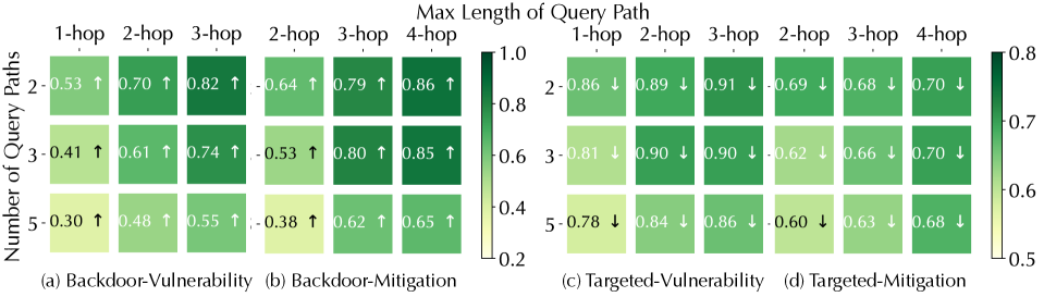
### Visual Description
## Heatmap Matrix: Performance Metrics for Backdoor and Targeted Vulnerability/Mitigation
### Overview
The image presents a matrix of four heatmaps, labeled (a) through (d), illustrating performance metrics across different query configurations. The charts analyze the relationship between the "Number of Query Paths" (rows: 2, 3, 5) and the "Max Length of Query Path" (columns: 1-hop, 2-hop, 3-hop, 4-hop). The data is divided into two categories: "Backdoor" (a, b) and "Targeted" (c, d), with each category showing both "Vulnerability" and "Mitigation" metrics.
### Components/Axes
* **Y-Axis (Left):** "Number of Query Paths" with discrete values: 2, 3, and 5.
* **X-Axis (Top):** "Max Length of Query Path" with discrete values:
* For (a) and (b): 1-hop, 2-hop, 3-hop.
* For (c) and (d): 2-hop, 3-hop, 4-hop.
* **Legends:**
* **Left Legend (for a & b):** A color scale ranging from 0.2 (light yellow-green) to 1.0 (dark green).
* **Right Legend (for c & d):** A color scale ranging from 0.5 (light yellow-green) to 0.8 (dark green).
* **Symbols:**
* Charts (a) and (b) contain upward-pointing arrows ($\uparrow$) in every cell.
* Charts (c) and (d) contain downward-pointing arrows ($\downarrow$) in every cell.
### Detailed Analysis
#### (a) Backdoor-Vulnerability
* **Trend:** Values increase as the hop count increases (left to right) and decrease as the number of query paths increases (top to bottom).
* **Data Points:**
* Row 2: 0.53 (1-hop), 0.70 (2-hop), 0.82 (3-hop)
* Row 3: 0.41 (1-hop), 0.61 (2-hop), 0.74 (3-hop)
* Row 5: 0.30 (1-hop), 0.48 (2-hop), 0.55 (3-hop)
#### (b) Backdoor-Mitigation
* **Trend:** Similar to (a), values increase with hop count and decrease with the number of query paths.
* **Data Points:**
* Row 2: 0.64 (1-hop), 0.79 (2-hop), 0.86 (3-hop)
* Row 3: 0.53 (1-hop), 0.80 (2-hop), 0.85 (3-hop)
* Row 5: 0.38 (1-hop), 0.62 (2-hop), 0.65 (3-hop)
#### (c) Targeted-Vulnerability
* **Trend:** Values are consistently high. There is a slight increase as hop count increases and a slight decrease as the number of query paths increases.
* **Data Points:**
* Row 2: 0.86 (2-hop), 0.89 (3-hop), 0.91 (4-hop)
* Row 3: 0.81 (2-hop), 0.90 (3-hop), 0.90 (4-hop)
* Row 5: 0.78 (2-hop), 0.84 (3-hop), 0.86 (4-hop)
#### (d) Targeted-Mitigation
* **Trend:** Values are lower than in (c). There is a slight increase as hop count increases and a slight decrease as the number of query paths increases.
* **Data Points:**
* Row 2: 0.69 (2-hop), 0.68 (3-hop), 0.70 (4-hop)
* Row 3: 0.62 (2-hop), 0.66 (3-hop), 0.70 (4-hop)
* Row 5: 0.60 (2-hop), 0.63 (3-hop), 0.68 (4-hop)
### Key Observations
* **Metric Sensitivity:** The "Backdoor" metrics (a, b) show a wider variance (0.30 to 0.86) compared to the "Targeted" metrics (c, d), which are more tightly clustered (0.60 to 0.91).
* **Inverse Relationship:** In all four charts, increasing the "Number of Query Paths" (moving down the rows) consistently results in lower values, suggesting that higher path counts may dilute the effect or increase the difficulty of the task.
* **Positive Correlation with Hops:** Increasing the "Max Length of Query Path" (moving across the columns) consistently results in higher values, suggesting that longer paths are more effective or impactful for both vulnerability and mitigation.
### Interpretation
The data suggests that the system's vulnerability and mitigation effectiveness are highly dependent on the geometry of the query path.
* **Backdoor Analysis:** The "Backdoor" vulnerability (a) is significantly mitigated by the "Backdoor-Mitigation" (b) strategy, as evidenced by the higher values in (b) compared to (a) across corresponding cells. The upward arrows ($\uparrow$) likely denote that higher values are "better" or "more successful" in this context.
* **Targeted Analysis:** The "Targeted-Vulnerability" (c) shows very high values (approaching 0.9), indicating the system is highly susceptible to targeted attacks. The "Targeted-Mitigation" (d) values are lower than (c), which, given the downward arrows ($\downarrow$), suggests that the mitigation strategy is successfully reducing the vulnerability metric.
* **Summary:** The system is more vulnerable to targeted attacks than backdoor attacks, but the mitigation strategies appear to be functioning as intended by reducing the vulnerability metrics in the targeted scenario.
</details>
Figure 14: ROAR ${}_{\mathrm{co}}$ performance (MRR) under different query structures in Figure 5, indicated by the change ( $\uparrow$ or $\downarrow$ ) before and after the attacks.