2305.10459

## AnalogNAS: A Neural Network Design Framework for Accurate Inference with Analog In-Memory Computing Hadjer Benmeziane ∗ , Corey Lammie † , Irem Boybat † , Malte Rasch ‡ ,Manuel Le Gallo † , Hsinyu Tsai § , Ramachandran Muralidhar , Smail Niar , Ouarnoughi Hamza , Vijay Narayanan ‡ ∗ ∗ ‡ , † ‡ Abu Sebastian and Kaoutar El Maghraoui , ∗ Univ. Polytechnique Hauts-de-France, CNRS, UMR 8201 - LAMIH, F-59313 Valenciennes, France † IBM Research Europe, 8803 R¨ uschlikon, Switzerland ‡ IBM T. J. Watson Research Center, Yorktown Heights, NY 10598, USA § IBM Research Almaden, 650 Harry Road, San Jose, CA USA Abstract -The advancement of Deep Learning (DL) is driven by efficient Deep Neural Network (DNN) design and new hardware accelerators. Current DNN design is primarily tailored for general-purpose use and deployment on commercially viable platforms. Inference at the edge requires low latency, compact and power-efficient models, and must be cost-effective. Digital processors based on typical von Neumann architectures are not conducive to edge AI given the large amounts of required data movement in and out of memory. Conversely, analog/mixedsignal in-memory computing hardware accelerators can easily transcend the memory wall of von Neuman architectures when accelerating inference workloads. They offer increased areaand power efficiency, which are paramount in edge resourceconstrained environments. In this paper, we propose AnalogNAS , a framework for automated DNN design targeting deployment on analog In-Memory Computing (IMC) inference accelerators. We conduct extensive hardware simulations to demonstrate the performance of AnalogNAS on State-Of-The-Art (SOTA) models in terms of accuracy and deployment efficiency on various Tiny Machine Learning (TinyML) tasks. We also present experimental results that show AnalogNAS models achieving higher accuracy than SOTA models when implemented on a 64-core IMC chip based on Phase Change Memory (PCM). The AnalogNAS search code is released 1 . Index Terms -Analog AI, Neural Architecture Search, Optimization, Edge AI, In-memory Computing ## I. INTRODUCTION W ITH the growing demands of real-time DL workloads, today's conventional cloud-based AI deployment approaches do not meet the ever-increasing bandwidth, realtime, and low-latency requirements. Edge computing brings storage and local computations closer to the data sources produced by the sheer amount of Internet of Things (IoT) objects, without overloading network and cloud resources. As © 2023 IEEE. Personal use of this material is permitted. Permission from IEEE must be obtained for all other uses, in any current or future media, including reprinting/republishing this material for advertising or promotional purposes, creating new collective works, for resale or redistribution to servers or lists, or reuse of any copyrighted component of this work in other works. 1 https://github.com/IBM/analog-nas DNNs are becoming more memory and compute intensive, edge AI deployments on resource-constrained devices pose significant challenges. These challenges have driven the need for specialized hardware accelerators for on-device Machine Learning (ML) and a plethora of tools and solutions targeting the development and deployment of power-efficient edge AI solutions. One such promising technology for edge hardware accelerators is analog-based IMC, which is herein referred to as analog IMC . Analog IMC [1] can provide radical improvements in performance and power efficiency, by leveraging the physical properties of memory devices to perform computation and storage at the same physical location. Many types of memory devices, including Flash memory, PCM, and Resistive Random Access Memory (RRAM), can be used for IMC [2]. Most notably, analog IMC can be used to perform Matrix-Vector Mutliplication (MVM) operations in O (1) time complexity [3], which is the most dominant operation used for DNN acceleration. In this novel approach, the weights of linear, convolutional, and recurrent DNN layers are mapped to crossbar arrays (tiles) of Non-Volatile Memory (NVM) elements. By exploiting basic Kirchhoff's circuit laws, MVMs can be performed by encoding inputs as Word-Line (WL) voltages and weights as device conductances. For most computations, this removes the need to pass data back and forth between Central Processing Units (CPUs) and memory. This back and forth data movement is inherent in traditional digital computing architectures, and is often referred to as the von Neumann bottleneck . Because there is greatly reduced movement of data, tasks can be performed in a fraction of the time, and with much less energy. NVM crossbar arrays and analog circuits, however, have inherent non-idealities, such as noise, temporal conductance drift, and non-linear errors, which can lead to imprecision and noisy computation [4]. These effects need to be properly quantified and mitigated to ensure the high accuracy of DNN models. 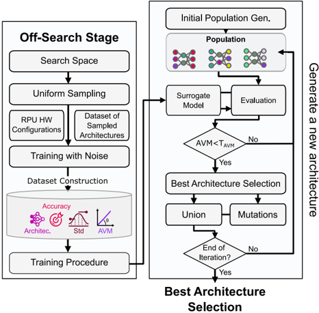In addition to the hardware constraints that are prevalent in edge devices, there is the added complexity of designing DNN Fig. 1. The effect of PCM conductance drift after one day on standard CNN architectures and one architecture ( AnalogNAS\_T500 ) obtained using HW-NAS, evaluated using CIFAR-10. FP refers to the original network accuracy, and 1-day to the simulated analog network accuracy after 1-day device drift. <details> <summary>Image 1 Details</summary>  ### Visual Description ## Scatter Plot: Network Accuracy vs. Parameters ### Overview The image is a scatter plot comparing the test set accuracy of different neural network architectures against the number of network parameters. The plot shows the accuracy of each network under two conditions, "FP" and "1-day", and includes a note about the gap between these conditions for robust networks. ### Components/Axes * **X-axis:** Number of Network Parameters (logarithmic scale). Axis markers are at approximately 10^6 and 10^7. * **Y-axis:** Test Set Accuracy (%). Axis markers are at 80.0, 82.5, 85.0, 87.5, 90.0, 92.5, 95.0, 97.5, and 100.0. * **Legend:** Located on the right side of the plot. * **Network:** Resnet20, Resnet32, Resnext29, Wide Resnet, AnalogNAS\_T500 * **FP:** Resnet20 (hollow hexagon), Resnet32 (hollow square), Resnext29 (light green X), Wide Resnet (hollow diamond), AnalogNAS\_T500 (hollow circle) * **1-day:** Resnet20 (solid red hexagon), Resnet32 (solid cyan square), Resnext29 (solid green X), Wide Resnet (solid yellow diamond), AnalogNAS\_T500 (solid purple circle) * **Annotation:** "For robust networks, this gap is minimized" with a vertical line indicating the gap. ### Detailed Analysis * **Resnet20:** * FP: Accuracy ~87.0% at parameter count ~ 10^6 * 1-day: Accuracy ~83.5% at parameter count ~ 10^6 * **Resnet32:** * FP: Accuracy ~94.5% at parameter count ~ 10^6 * 1-day: Accuracy ~90.5% at parameter count ~ 10^6 * **Resnext29:** * FP: Accuracy ~95.5% at parameter count ~ 10^7 * 1-day: Accuracy ~92.5% at parameter count ~ 10^7 * **Wide Resnet:** * FP: Accuracy ~95.0% at parameter count ~ 10^7 * 1-day: Accuracy ~93.0% at parameter count ~ 10^7 * **AnalogNAS\_T500:** * FP: Accuracy ~94.5% at parameter count ~ 10^6 * 1-day: Accuracy ~92.5% at parameter count ~ 10^6 * **Trends:** * For each network architecture, the "FP" accuracy is higher than the "1-day" accuracy. * The number of parameters for Resnet20, Resnet32, and AnalogNAS_T500 is approximately 10^6. * The number of parameters for Resnext29 and Wide Resnet is approximately 10^7. ### Key Observations * The gap between "FP" and "1-day" accuracy varies across different network architectures. * The annotation suggests that for more robust networks, this gap is smaller. * The networks with a higher number of parameters (Resnext29, Wide Resnet) generally achieve higher accuracy. ### Interpretation The plot illustrates the trade-off between network size (number of parameters) and test set accuracy for different neural network architectures. The difference in accuracy between the "FP" and "1-day" conditions likely represents a measure of robustness or generalization ability. The annotation highlights that robust networks tend to minimize this accuracy gap. The data suggests that increasing the number of parameters generally leads to higher accuracy, but the choice of network architecture also plays a significant role in achieving optimal performance and robustness. </details> architectures which are optimized for the edge on a variety of hardware platforms. This requires hardware-software co-design approaches to tackle this complexity, as manually-designed architectures are often tailored for specific hardware platforms. For instance, MobileNet [5] uses a depth-wise separable convolution that enhances CPU performance but is inefficient for Graphics Processing Unit (GPU) parallelization [6]. These are bespoke solutions that are often hard to implement and generalize to other platforms. HW-NAS [7] is a promising approach that seeks to automatically identify efficient DNN architectures for a target hardware platform. In contrast to traditional Neural Architecture Search (NAS) approaches that focus on searching for the most accurate architectures, HW-NAS searches for highly accurate models while optimizing hardware-related metrics. Existing HW-NAS strategies cannot be readily used with analog IMC processors without significant modification for three reasons: (i) their search space contains operations and blocks that are not suitable for analog IMC, (ii) lack of a benchmark of hardwareaware trained architectures, and (iii) their search strategy does not include noise injection and temporal drift on weights. To address these challenges, we propose AnalogNAS , a novel HW-NAS strategy to design dedicated DNN architectures for efficient deployment on edge-based analog IMC inference accelerators. This approach considers the inherent characteristics of analog IMC hardware in the search space and search strategy. Fig. 1 depicts the necessity of our approach. As can be seen, when traditional DNN architectures are deployed on analog IMC hardware, non-idealities, such as conductance drift, drastically reduce network performance. Networks designed by AnalogNAS are extremely robust to these non-idealities and have much fewer parameters compared to equivalently-robust traditional networks. Consequently, they have reduced resource utilization. Our specific contributions can be summarized as follows: - We design and construct a search space for analog IMC, which contains ResNet-like architectures, including ResNext [8] and Wide-ResNet [9], with blocks of varying widths and depths; - We train a collection of networks using Hardware-Aware (HWA) training for image classification, Visual Wake Words (VWW), and Keyword Spotting (KWS) tasks. Using these networks, we build a surrogate model to rank the architectures during the search and predict robustness to conductance drift; - We propose a global search strategy that uses evolutionary search to explore the search space and efficiently finds the right architecture under different constraints, including the number of network parameters and analog tiles; - We conduct comprehensive experiments to empirically demonstrate that AnalogNAS can be efficiently utilized to carry out architecture search for various edge tiny applications, and investigate what attributes of networks make them ideal for implementation using analog AI; - We validate a subset of networks on hardware using a 64-core IMC chip based on PCM. The rest of the paper is structured as follows. In Section II, we present related work. In Section III, relevant notations and terminology are introduced. In Section IV, the search space and surrogate model are presented. In Section V, the search strategy is presented. In Section VI, the methodology for all experiments is discussed. The simulation results are presented in Section VI-B, along with the hardware validation and performance estimation in Section VII. The results are discussed in Section VIII. Section IX concludes the paper. ## II. RELATED WORK ## A. NAS for TinyML HW-NAS has been successfully applied to a variety of edge hardware platforms [7], [10] used to deploy networks for TinyMLPerf tasks [11] such as image classification, VWW, KWS, and anomaly detection. MicroNets [12] leverages NAS for DL model deployment on micro-controllers and other embedded systems. It utilizes a differentiable search space [13] to find efficient architectures for different TinyMLPerf tasks. For each task, the search space is an extension of current SOTA architectures. µ -nas [14] includes memory peak usage and a number of other parameters as constraints. Its search strategy combines aging evolution and Bayesian optimization to estimate the objectives and explore a granular search space efficiently. It constructs its search space from a standard CNN and modifies the operators' hyper-parameters and a number of layers. ## B. NAS for Mixed-Signal IMC Accelerators Many works [15]-[18] target IMC accelerators using HW-NAS. FLASH [15] uses a small search space inspired by DenseNet [19] and searches for the number of skip connections that efficiently satisfy the trade-off between accuracy, latency, energy consumption, and chip area. Its surrogate model uses linear regression and the number of skip connections to predict model accuracy. NAS4RRAM [17] uses HW-NAS to find an efficient DNN for a specific RRAMbased accelerator. It uses an evolutionary algorithm, trains each sampled architecture without HWA training, and evaluates each network on a specific hardware instance. NACIM [16] uses coexploration strategies to find the most efficient architecture and the associated hardware platform. For each sampled architecture, networks are trained considering noise variations. This approach is limited by using a small search space due to the high time complexity of training. UAE [18] uses a Monte-Carlo simulation-based experimental flow to measure the device uncertainty induced to a handful of DNNs. Similar to NACIM [16], evaluation is performed using HWA training with noise injection. AnalogNet [20] extends the work of Micronet by converting their final models to analog-friendly models, replacing depthwise convolutions with standard convolutions and tuning hyperparameters. Compared to the above-mentioned SOTA HW-NAS strategies, our AnalogNAS is better tailored to analog IMC hardware for two reasons: (i) Our search space is much larger and more representative, featuring resnet-like connections. This enables us to answer the key question of what architectural characteristics are suitable for analog IMC which cannot be addressed with small search spaces. (ii) We consider the inherent characteristics of analog IMC hardware directly in the objectives and constraints of our search strategy in addition to noise injection during the HWA training as used by existing approaches. ## III. PRELIMINARIES ## A. 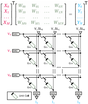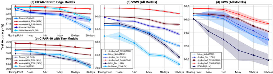Analog IMC Accelerator Mechanisms Analog IMC accelerators are capable of performing MVM operations Y T = X T W using the laws of physics, where W is an M × N matrix, X is a M × 1 vector, and Y is a N × 1 vector. When arranged in a crossbar configuration, M × N , NVM devices can be used to compute MVM operations. This is done by encoding elements of X as WL voltages, denoted using V , and elements of W as conductances of the unit cells, denoted using G . Negative conductance states cannot be directly encoded/represented using NVM devices. Consequently, differential weight mapping schemes are commonly employed, where either positive weights, i.e., W + = max( W , 0) , and negative weights, i.e., W -= -min( W , 0) , are encoded within unit cells, using alternate columns, or on different tiles [3]. The analog computation, i.e., I = VG is performed, where the current flow to the end of the N -th column is I N = ∑ M i =0 G i,N V i . Typically, Digital-to-Analog Converters (DACs) are required to encode WL voltages and Analog-toDigital Converters (ADCs) are required to read the output currents of each column. The employed analog IMC tile, its weight mapping scheme, and computation mechanism are depicted in Fig. 2. ## B. Temporal Drift of Non-Volatile Memory Devices Many types of NVM devices, most prominantly, PCM, exhibit temporal evolution of the conductance values referred to as the conductance drift. This poses challenges for maintaining synaptic weights reliably [2]. Conductance drift is most commonly modelled using Eq. (1), as follows: <!-- formula-not-decoded --> where G ( t 0 ) is the conductance at time t 0 and ν is the drift exponent. In practice, conductance drift is highly stochastic because ν depends on the programmed conductance state and varies across devices. Consequently, when reporting the network accuracy at a given time instance (after device programming), it is computed across multiple experiment instances (trials) to properly capture the amount of accuracy variations. ## C. HWA-training and analog hardware accuracy evaluation simulation To simulate training and inference on analog IMC accelerators, the IBM Analog Hardware Acceleration Kit (AIHWKIT) [21] is used. The AIHWKIT is an open-source Python toolkit for exploring and using the capabilities of inmemory computing devices in the context of artificial intelligence and has been used for HWA training of standard DNNs with hardware-calibrated device noise and drift models [22]. ## D. Hardware-aware Neural Architecture Search (HW-NAS) HW-NAS refers to the task of automatically finding the most efficient DNN for a specific dataset and target hardware platform. HW-NAS approaches often employ black-box optimization methods such as evolutionary algorithms [23], reinforcement learning [24], [25], and Bayesian optimization [26], [27]. The optimization problem is either cast as a constrained or multi-objective optimization [7]. In AnalogNAS, we chose constrained optimization over multi-objective optimization for several reasons. First, constrained optimization is more computationally efficient than multi-objective optimization, which is important in the context of HW-NAS, to allow searching a large search space in a practical time frames. Multi-objective optimization is computationally expensive and can result in a Fig. 2. Employed analog IMC tile and weight mapping scheme. <details> <summary>Image 2 Details</summary>  ### Visual Description ## Matrix Multiplication Circuit Diagram ### Overview The image presents a circuit diagram illustrating a matrix multiplication operation. It shows an array of unit cells, each containing a memristor, arranged in a grid. The diagram also includes input voltages (V0 to VM), digital-to-analog converters (DACs), analog-to-digital converters (ADCs), and output currents (I0 to IN). The matrix multiplication is represented mathematically at the top of the diagram. ### Components/Axes * **Mathematical Representation (Top):** * **Left Matrix (X):** A column vector with elements X0, X1, ..., XM. The vector is transposed (T). The elements are colored red. * **Middle Matrix (W):** A matrix with elements W00, W01, ..., W0N, W10, W11, ..., W1N, ..., WM0, WM1, ..., WMN. * **Right Matrix (Y):** A column vector with elements Y0, Y1, ..., YN. The vector is transposed (T). The elements are colored blue. * The equation represents X * W = Y. * **Circuit Diagram (Center):** * **Input Voltages:** V0, V1, ..., VM. Each connected to a DAC. * **DACs:** Digital-to-Analog Converters, converting digital inputs to analog voltages. * **Memristor Array:** A grid of memristors, each labeled G00, G01, ..., G0N, G10, G11, ..., G1N, ..., GM0, GM1, ..., GMN. * **Output Currents:** I0, I1, ..., IN. Each connected to an ADC. The elements are colored blue. * **ADCs:** Analog-to-Digital Converters, converting analog currents to digital outputs. * **Vertical Lines:** Labeled V_SL0, V_SL1, ..., V_SLN. * **Legend (Bottom-Left):** * "Unit Cell" is represented by a rectangular block with a diagonal line. ### Detailed Analysis or Content Details * **Matrix Multiplication:** The mathematical representation at the top shows the matrix multiplication being performed by the circuit. The input vector X is multiplied by the weight matrix W to produce the output vector Y. * **Circuit Operation:** The input voltages V0 to VM are converted to analog signals by the DACs. These voltages are applied to the rows of the memristor array. The memristors act as variable resistors, and their conductances (G) represent the elements of the weight matrix W. The output currents I0 to IN are proportional to the product of the input voltages and the memristor conductances. These currents are converted to digital signals by the ADCs. * **Unit Cell:** Each unit cell in the array contains a memristor. The conductance of the memristor can be programmed to represent a specific weight value. * **Grid Structure:** The memristors are arranged in a grid, with each row corresponding to an input voltage and each column corresponding to an output current. The vertical lines are labeled V_SL0, V_SL1, ..., V_SLN. ### Key Observations * The circuit diagram implements matrix multiplication using a memristor array. * The memristor conductances represent the elements of the weight matrix. * The input voltages represent the elements of the input vector. * The output currents represent the elements of the output vector. ### Interpretation The diagram illustrates a hardware implementation of matrix multiplication using memristors. This approach offers potential advantages in terms of speed, power consumption, and area compared to traditional digital implementations. The memristor array allows for parallel computation of the matrix multiplication, which can significantly speed up the process. The use of analog signals also reduces the power consumption compared to digital circuits. This type of architecture is relevant for applications such as machine learning, where matrix multiplication is a fundamental operation. The diagram shows how the mathematical operation is mapped onto a physical circuit, highlighting the relationship between the abstract mathematical concept and its concrete implementation. 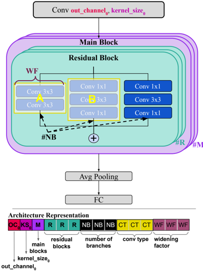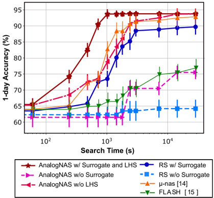</details> Fig. 3. Resnet-like macro architecture. <details> <summary>Image 3 Details</summary>  ### Visual Description ## Diagram: Convolutional Neural Network Block Diagram ### Overview The image is a block diagram illustrating the architecture of a convolutional neural network (CNN). It depicts the flow of data through different layers and blocks, including convolutional layers, residual blocks, pooling layers, and fully connected layers. The diagram also includes an "Architecture Representation" section that summarizes the network's structure using abbreviations. ### Components/Axes * **Top Block:** "Conv out\_channel₀, kernel\_size₀" (Gray rounded rectangle) * **Main Block:** A series of nested rounded rectangles, labeled "Main Block" (Purple outline). * **Residual Block:** Located within the Main Block (Teal outline). * **Convolutional Layers:** Represented as rectangles labeled "Conv 1x1", "Conv 3x3", and "Co 3x3". These are arranged in parallel within the Residual Block. * **Addition Operator:** A circled plus sign (+) indicating element-wise addition. * **Avg Pooling:** A gray rectangle labeled "Avg Pooling". * **FC:** A gray rectangle labeled "FC" (Fully Connected Layer). * **Architecture Representation:** A horizontal sequence of colored blocks with abbreviations. * OC₀KS₀ (Red): Represents out\_channel₀ and kernel\_size₀. * M (Purple): Represents main blocks. * R (Green): Represents residual blocks. * NB (Black): Represents the number of branches. * CT (Yellow): Represents conv type. * WF (Teal): Represents the widening factor. * **Arrows:** Indicate the flow of data between the blocks and layers. * **Labels:** * WF: Widening Factor * \#NB: Number of Branches * \#R: Number of Residual Blocks * \#M: Number of Main Blocks ### Detailed Analysis * **Top Block:** The diagram starts with a convolutional layer, denoted as "Conv out\_channel₀, kernel\_size₀". * **Main Block:** The data flows into the "Main Block," which contains multiple "Residual Blocks." The number of main blocks is indicated by #M. * **Residual Block:** Each "Residual Block" contains parallel convolutional layers. One branch contains "Conv 3x3", "Co 3x3", and "Conv 3x3" (yellow outline). Another branch contains "Conv 1x1", "Conv 3x3", and "Conv 1x1" (blue outline). The output of these branches is added together using the addition operator (+). The number of residual blocks is indicated by #R. * **Number of Branches:** The number of branches is indicated by #NB. * **Widening Factor:** The widening factor is indicated by WF. * **Avg Pooling:** After the "Residual Block," the data passes through an "Avg Pooling" layer. * **FC:** Finally, the data is fed into a "FC" (Fully Connected) layer. * **Architecture Representation:** This section provides a compact representation of the network's architecture. It shows the sequence of main blocks (M), residual blocks (R), number of branches (NB), conv type (CT), and widening factor (WF). The number of each type of block is indicated by the number of consecutive blocks of the same color. ### Key Observations * The diagram highlights the use of residual connections in the network architecture. * The "Architecture Representation" provides a concise summary of the network's structure. * The diagram shows the flow of data through different layers and blocks, making it easy to understand the network's architecture. ### Interpretation The diagram illustrates a CNN architecture that utilizes residual connections to improve performance. The residual blocks allow the network to learn more complex features by adding the input of a block to its output. The "Architecture Representation" provides a way to easily specify and compare different network architectures. The diagram is useful for understanding the structure and flow of data in the CNN. </details> large number of non-dominated solutions that can be difficult to interpret. Secondly, by using constrained optimization, we can explicitly incorporate the specific constraints of the analog hardware in our search strategy. This enables us to find DNN architectures that are optimized for the unique requirements and characteristics of analog IMC hardware, rather than simply optimizing for multiple objectives. ## IV. ANALOG-NAS The objective of AnalogNAS is to find an efficient network architecture under different analog IMC hardware constraints. AnalogNAS comprises three main components: (i) a resnetlike search space, (ii) an analog-accuracy surrogate model, and (iii) an evolutionary-based search strategy. We detail each component in the following subsections. ## A. Resnet-like Search Space Resnet-like architectures have inspired many manually designed SOTA DL architectures, including Wide ResNet [9] and EfficientNet [28]. Their block-wise architecture offers a flexible and searchable macro-architecture for NAS [29]. Resnet-like architectures can be implemented efficiently using IMC processors, as they are comprised of a large number of MVM and element-wise operations. Additionally, due to the highly parallel nature of IMC, Resnet architectures can get free processing of additional input/output channels. This makes Resnet-like architectures highly amenable to analog implementation. Fig. 3 depicts the macro-architecture used to construct all architectures in our search space. The architecture consists of a series of M distinct main blocks. Each main block contains R residual blocks. The residual blocks use skip connections with or without downsampling. Downsampling is performed using 1x1 convolution layers when required, i.e., when the input size does not match the output size. The residual block can have B branches. Each branch uses a convolution block. We used different types of convolution blocks to allow the search space to contain all standard architectures such as Resnets [30], ResNext [8], and Wide Resnets [9]. The standard convolution blocks used in Resnets, commonly referred to as BottleNeckBlock and BasicBlock , are denoted as A and B respectively. We include variants of A and B in which we inverse the order of the ReLU and Batch normalization operations. The resulting blocks are denoted as C and D. Table I summarizes the searchable hyper-parameters and their respective ranges. The widening factor scales the width of the residual block. We sample architectures with different depths by changing the number of main and residual blocks. The total size of the search space is approximately 73B architectures. The larger architecture would contain 240 convolutions and start from an output channel of 128 multiplying that by 4 for every 16 blocks. ## B. Analog-accuracy Surrogate Model - 1) Evaluation Criteria: To efficiently explore the search space, a search strategy requires evaluating the objectives of each sampled architecture. Training the sampled architectures is very time-consuming; especially when HWA retraining is performed, as noise injection and I/O quantization modeling greatly increases the computational complexity. Consequently, we build a surrogate model capable of estimating the objectives of each sampled architecture in IMC devices. To find architectures that maximize accuracy, stability, and resilience against IMC noise and drift characteristics, we have identified the following three objectives. - a) The 1-day accuracy: is the primary objective that most NAS algorithms aim to maximize. It measures the performance of an architecture on a given dataset. When weights are encoded using IMC devices, the accuracy of the architecture can drop over time due to conductance drift. Therefore, we have selected the 1-day accuracy as a metric to measure the architecture's performance. - b) The Accuracy Variation over One Month (AVM): is the difference between the 1-month and 1-sec accuracy. This objective is essential to measure the robustness over a fixed time duration. A 30-day period allows for a reasonable trade-off between capturing meaningful accuracy changes and avoiding short-term noise and fluctuations that may not reflect long-term trends. - c) The 1-day accuracy standard deviation: measures the variation of the architecture's performance across experiments, as discussed in Section III-B. A lower standard deviation indicates that the architecture produces consistent results on hardware deployments, which is essential for real-world applications. TABLE I SEARCHABLE HYPER-PARAMETERS AND THEIR RESPECTIVE RANGES. | Hyper- parameter | Definition | Range | |--------------------|-----------------------------------------------------------------------------------------------------------------------------------------------------------------------------------------------------------------------------|---------------------------------------------------------------------------------------------------------------------------------------------------------------------| | OC 0 | First layer's output channel First layer's kernel size Number of main blocks Number of residual block per main block Number of branches per main block Convolution block type per main block Widening factor per main block | Discrete Uniform [8, 128] Discrete Uniform [3, 7] Discrete Uniform [1, 5] Discrete Uniform [1, 16] Discrete Uniform [1, 12] Uniform Choice [A; B; C; Uniform [1, 4] | | KS 0 | | | | M | | | | R* | | | | B* | | | | CT* | | D] | | WF* | | | To build the surrogate model, we follow two steps: Dataset creation and Model training: - 2) Dataset Creation: The surrogate model will predict the rank based on the 1-day accuracy and estimates the AVM and 1-day accuracy standard deviation using the Mean Squared Error (MSE). Since the search space is large, care has to be taken when sampling the dataset of architectures that will be used to train the surrogate model. 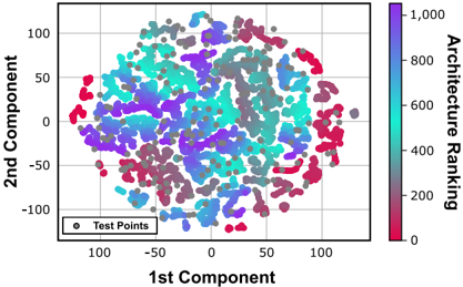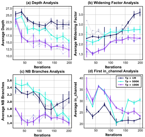The architectures of the search space are sampled using two methods: (i) Latin Hypercube Sampling (LHS) [31] and (ii) NAS with full training. A more detailed description of the AnalogNAS algorithm is presented in Section V. We use LHS to sample architectures distributed evenly over the search space. This ensures good overall coverage of different architectures and their accuracies. NAS with full training is performed using an evolutionary algorithm to collect high-performance architectures. This ensures good exploitation when reaching well-performing regions. In Fig. 4, we present a visualization of the search space coverage, which does not show any clustering of similarly performing architectures at the edge of the main cloud of points. Thus, it is not evident that architectures with similar performance are located close to each other in the search space. This suggests that traditional search methods that Fig. 4. t-Distributed Stochastic Neighbor Embedding (t-SNE) visualization of the sampled architectures for CIFAR-10. <details> <summary>Image 4 Details</summary>  ### Visual Description ## Scatter Plot: Architecture Ranking by Components ### Overview The image is a scatter plot showing the distribution of data points in a two-dimensional space defined by "1st Component" and "2nd Component". The data points are colored according to an "Architecture Ranking" scale, ranging from red (low) to purple (high). Gray dots are overlaid on the colored data points, labeled as "Test Points". ### Components/Axes * **X-axis (1st Component):** Ranges from approximately -100 to 100, with gridlines at intervals of 50. * **Y-axis (2nd Component):** Ranges from approximately -100 to 100, with gridlines at intervals of 50. * **Color Scale (Architecture Ranking):** A vertical color bar on the right side of the plot represents the "Architecture Ranking". The scale ranges from 0 (red) to 1000 (purple), with intermediate colors of gray, teal, and blue. * **Legend:** Located in the bottom-left corner, indicating that the gray dots represent "Test Points". ### Detailed Analysis * **Data Point Distribution:** The data points form a roughly circular cluster, with higher density in the central region. * **Color Gradient:** The color gradient indicates that lower architecture rankings (red) are concentrated on the right side of the plot, while higher rankings (purple) are more prevalent in the upper and central regions. * **Test Points:** The gray "Test Points" are scattered throughout the plot, appearing to overlay the colored data points. ### Key Observations * There is a clear correlation between the position of data points and their architecture ranking. * The distribution of data points is not uniform, with some areas having higher concentrations of specific rankings. * The "Test Points" appear to be a subset of the overall data, possibly representing a validation or test set. ### Interpretation The scatter plot visualizes the relationship between two components and the architecture ranking of data points. The clustering of points with similar rankings suggests that these components are relevant features for distinguishing between different architectures. The color gradient indicates a trend where higher component values are associated with higher architecture rankings. The "Test Points" likely represent a subset of the data used to evaluate the performance of a model or algorithm. The plot could be used to identify promising architectures or to understand the feature space of the underlying data. 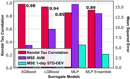</details> Fig. 5. Surrogate models comparison. <details> <summary>Image 5 Details</summary>  ### Visual Description ## Bar Chart: Surrogate Model Performance ### Overview The image is a bar chart comparing the performance of different surrogate models (XGBoost, LGBoost, MLP, and MLP Ensemble) based on Kendal Tau Correlation, MSE AVM (Mean Squared Error Average Variance Method), and MSE 1-day STD-DEV (Mean Squared Error 1-day Standard Deviation). The chart uses two y-axes: one for Kendal Tau Correlation (left) and another for Mean Squared Error (right). ### Components/Axes * **X-axis:** Surrogate Models (XGBoost, LGBoost, MLP, MLP Ensemble) * **Left Y-axis:** Kendal Tau Correlation, ranging from 0.0 to 1.0 * **Right Y-axis:** Mean Squared Error, ranging from 0.0 to 15.0 * **Legend:** Located in the center of the chart. * Red: Kendal Tau Correlation * Purple: MSE AVM * Teal: MSE 1-day STD-DEV ### Detailed Analysis Here's a breakdown of the data for each model: * **XGBoost:** * Kendal Tau Correlation: 0.98 (Red bar) * MSE AVM: Approximately 0.35 (Purple bar) * MSE 1-day STD-DEV: Approximately 0.05 (Teal bar) * **LGBoost:** * Kendal Tau Correlation: 0.94 (Red bar) * MSE AVM: Approximately 6.0 (Purple bar) * MSE 1-day STD-DEV: Approximately 0.1 (Teal bar) * **MLP:** * Kendal Tau Correlation: 0.85 (Red bar) * MSE AVM: Approximately 14.0 (Purple bar) * MSE 1-day STD-DEV: Approximately 5.5 (Teal bar) * **MLP Ensemble:** * Kendal Tau Correlation: 0.89 (Red bar) * MSE AVM: Approximately 13.0 (Purple bar) * MSE 1-day STD-DEV: Approximately 2.2 (Teal bar) ### Key Observations * XGBoost has the highest Kendal Tau Correlation (0.98) and the lowest MSE AVM and MSE 1-day STD-DEV. * MLP and MLP Ensemble have significantly higher MSE AVM values compared to XGBoost and LGBoost. * LGBoost has a relatively high Kendal Tau Correlation (0.94) but also a higher MSE AVM than XGBoost. * MSE 1-day STD-DEV is generally low for XGBoost and LGBoost, but higher for MLP and MLP Ensemble. ### Interpretation The chart suggests that XGBoost performs the best among the tested surrogate models, exhibiting the highest correlation and the lowest error rates. LGBoost also shows good correlation but has a higher MSE AVM compared to XGBoost. MLP and MLP Ensemble models have lower correlation and significantly higher MSE AVM, indicating potentially less accurate or stable performance. The MSE 1-day STD-DEV provides insight into the variability of the error, with XGBoost and LGBoost showing more consistent performance compared to MLP and MLP Ensemble. The ensemble method does not appear to improve the performance of the MLP model significantly. </details> rely on local optimization may not be effective in finding the best-performing architectures. Instead, population-based search strategies, which explore a diverse set of architectures, could be more effective in finding better-performing architectures. Our search strategy extracted 400 test points, and we found that architectures were distributed throughout the main cloud, indicating that our dataset covers a diverse portion of the search space, despite the limited size of only 1,000. Each sampled architecture is trained using different levels of weight noise and HWA training hyper-parameters using the AIHWKIT [21]. Specifically, we modify the standard deviation of the added weight noise between [0.1, 5.0] in increments of 0.1. The tile size was assumed to be symmetric and varied in [256, 512], representing 256-by-256 and 512-by-512 arrays respectively. Training with different configurations allowed us to generalize the use of the surrogate model across a range of IMC hardware configurations, and to increase the size of the constructed dataset. - 3) Model training: To train the surrogate model, we used a hinge pair-wise ranking loss [32] with margin m = 0 . 1 . The hinge loss, defined in Eq. (2), allows the model to learn the relative ranking order of architectures rather than the absolute accuracy values [32], [33]. <!-- formula-not-decoded --> a j refers to architectures indexed j , and y j to its corresponding 1-day accuracy. P ( a ) is the predicted score of architecture a . P ( a ) during training, the output score is trained to be correlated with the actual ranks of the architectures. Several algorithms were tested. After an empirical comparison, we adopted Kendall's Tau ranking correlation [34] as the direct criterion for evaluating ranking surrogate model performance. Fig. 5 shows the comparison using different ML algorithms to predict the rankings and AVMs. Our dataset is tabular. It contains each architecture and its corresponding features. XGBoost outperforms the different surrogate models in predicting the architectures' ranking order, the A VM of each architecture, and the 1-day standard deviation. Fig. 6. Overview of the AnalogNAS framework. <details> <summary>Image 6 Details</summary>  ### Visual Description ## Flow Diagram: Neural Architecture Search ### Overview The image presents a flow diagram illustrating a neural architecture search process. It consists of two main stages: an "Off-Search Stage" and a "Best Architecture Selection" stage. The diagram outlines the steps involved in generating and evaluating neural network architectures, ultimately selecting the best one based on certain criteria. ### Components/Axes **Off-Search Stage (Left Side):** * **Search Space:** The initial stage where the possible architectures are defined. * **Uniform Sampling:** A method for selecting architectures from the search space. * **RPU HW Configurations:** Hardware configurations for the architectures. * **Dataset of Sampled Architectures:** A collection of architectures sampled from the search space. * **Training with Noise:** Training the architectures with added noise. * **Dataset Construction:** Building a dataset from the trained architectures. * **Accuracy Metrics:** * **Architec.:** Represents the architecture itself (depicted as a network diagram). * **Std:** Standard deviation of performance (depicted as a bell curve). * **AVM:** Average value metric (depicted as an angle). * **Training Procedure:** The process of training the architectures. **Best Architecture Selection (Right Side):** * **Initial Population Gen.:** Generating an initial population of architectures. * **Population:** A set of architectures (depicted as network diagrams with different colored nodes). * **Surrogate Model:** A model used to approximate the performance of architectures. * **Evaluation:** Evaluating the performance of the architectures. * **AVM < T_AVM?:** A decision point comparing the average value metric (AVM) to a threshold (T_AVM). * **Yes:** If AVM is less than T_AVM, proceed to "Best Architecture Selection." * **No:** If AVM is not less than T_AVM, loop back to "Population" to generate a new architecture. * **Best Architecture Selection:** Selecting the best architecture from the population. * **Union:** Combining architectures. * **Mutations:** Introducing changes to the architectures. * **End of Iteration?:** A decision point to determine if the iteration is complete. * **Yes:** If the iteration is complete, end the process. * **No:** If the iteration is not complete, loop back to "Surrogate Model." * **Generate a new architecture:** Text on the right side of the diagram, indicating the iterative nature of the process. ### Detailed Analysis The diagram illustrates a two-stage process for neural architecture search. The "Off-Search Stage" focuses on generating a diverse dataset of architectures and training them with noise. This stage involves uniform sampling from the search space, training the sampled architectures, and constructing a dataset with accuracy metrics. The "Best Architecture Selection" stage iteratively refines the architecture by generating an initial population, evaluating their performance using a surrogate model, and selecting the best architectures based on the AVM metric. The process continues with union and mutation operations until the end of the iteration is reached. ### Key Observations * The diagram highlights the iterative nature of the architecture search process. * The use of a surrogate model suggests an attempt to reduce the computational cost of evaluating architectures. * The AVM metric plays a crucial role in selecting the best architectures. * The "Off-Search Stage" appears to be a preliminary step to generate a diverse dataset for the subsequent optimization process. ### Interpretation The flow diagram represents a neural architecture search algorithm that combines an initial exploration phase ("Off-Search Stage") with an iterative optimization phase ("Best Architecture Selection"). The "Off-Search Stage" aims to create a diverse dataset of architectures and their performance characteristics, which can then be used to train a surrogate model. The surrogate model is used to efficiently evaluate the performance of new architectures in the "Best Architecture Selection" stage. The algorithm iteratively refines the architecture by generating new populations, evaluating them using the surrogate model, and selecting the best architectures based on the AVM metric. The union and mutation operations introduce diversity and exploration into the search process. The comparison of AVM to T_AVM acts as a convergence criterion, determining when the algorithm has found a satisfactory architecture. The overall process aims to automate the design of neural network architectures, potentially leading to improved performance and efficiency compared to manually designed architectures. </details> ## V. SEARCH STRATEGY Fig. 6 depicts the overall search framework. Given a dataset and a hardware configuration readable by AIHWKIT, the framework starts by building the surrogate model presented in Section IV-B. Then, we use an optimized evolutionary search to efficiently explore the search space using the surrogate model. Similar to traditional evolutionary algorithms, we use real number encoding. Each architecture is encoded into a vector, and each element of the vector contains the value of the hyper-parameter, as listed in Table I. ## A. Problem Formulation Given the search space S , our goal is to find an architecture α , that maximizes the 1-day accuracy while minimizing the 1-day standard deviation, subject to constraints on the number of parameters and the AVM. The number of parameters is an important metric in IMC, because it directly impacts the amount of on-chip memory required to store the weights of a DNN. Eq. (3) formally describes the optimization problem as follows: <!-- formula-not-decoded --> ACC refers to the 1-day accuracy objective, σ denotes the 1-day accuracy's standard deviation, and ψ is the number of parameters. T p and T AVM are user-defined thresholds that correspond to the maximum number of parameters and AVM, respectively. ## B. Search Algorithm Our evolutionary search algorithm, i.e., AnalogNAS, is formally defined using Algorithm 1. AnalogNAS is an algorithm to find the most accurate and robust neural network architecture ## Algorithm 1 AnalogNAS algorithm. Input: Search space: S , RPU Configuration: rpu config , target task: task , population size: population size , AVM threshold: T AVM, parameter threshold: T p , number of iterations: N , time budget Output: Most efficient architecture for rpu config in S Begin D = sample( S , dataset size) HW Train( D , task ) AVMs = compute AVM( D ) surrogate model = XGBoost train(surrogate model, D , AVMs) ## repeat population = LHS(population size, T p ) AVMs, ranks = surrogate model(population) until AVMs > T AVM while i < N or time < time budget do top 50 = select(population, ranks) mutated = mutation(top 50, T p ) population = top 50 ⋃ mutated AVMs, ranks = surrogate model(population) ## end while return top 1 (population, ranks) for a given analog IMC configuration and task. The algorithm begins by generating a dataset of neural network architectures, which are trained on the task and evaluated using AIHWKIT. A surrogate model is then created to predict the efficiency of new architectures. The algorithm then generates a population of architectures using an LHS technique and selects the topperforming architectures to be mutated and generate a new population. The process is repeated until a stopping criterion is met, such as a maximum number of iterations or a time budget. Finally, the most robust architecture is returned. In the following, we detail how the population initialization, fitness evaluation, and mutations are achieved. - 1) Population Initialization: The search starts by generating an initial population. Using the LHS algorithm, we sample the population uniformly from the search space. LHS ensures that the initial population contains architectures with different architectural features. LHS is made faster with parallelization by dividing the sampling into multiple independent subsets, which can be generated in parallel using multiple threads. - 2) Fitness Evaluation: We evaluate the population using the aforementioned analog-accuracy surrogate model. In addition to the rankings, the surrogate model predicts the AVM of each architecture. As previously described, the AVM is used to gauge the robustness of a given network. If the AVM is below a defined threshold, T AVM, the architecture is replaced by a randomly sampled architecture. The new architecture is constrained to be sampled from the same hypercube dimension as the previous one. This ensures efficient exploration. - 3) Selection and Mutation: We select the top 50% architectures from the population using the predicted rankings. These architectures are mutated. The mutation functions are classified as follows: - a) Depth-related mutations: modify the depth of the architectures. Mutations include adding a main block, by increasing or decreasing M or a residual block R , or modifying the type of convolution block, i.e., { A,B,C,D } , for each main block. - b) Width-related mutations: modify the width of the architectures. Mutations include modifying the widening factor W of a main block or adding or removing a branch B , or modifying the initial output channel size of the first convolution, OC . - c) Other mutations: modify the kernel size of the first convolution, KS , and/or add skip connections,denoted using ST . Depth- and width-related mutations are applied with the same probability of 80%. The other mutations are applied with a 50% probability. In each class, the same probability is given to each mutation. The top 50% architectures in addition to the mutated architectures constitute the new population. For the remaining iterations, we verify the ranking correlation of the surrogate model. If the surrogate model's ranking correlation is degraded, we fine-tune the surrogate model with the population's architectures. The degradation is computed every 100 iterations. The surrogate model is tested on the population architectures after training them. It is fine-tuned if Kendall's tau correlation drops below 0.9. ## VI. EXPERIMENTS This section describes the experiments used to evaluate AnalogNAS on three tasks: CIFAR-10 image classification, VWW, and KWS. The AIHWKIT was used to perform hardware simulations. ## A. Experimental Setup - 1) Training Details: We detail the hyper-parameters used to train the surrogate model and different architectures on CIFAR-10, VWW, and KWS tasks. - a) Surrogate model training: We trained a surrogate model and dataset of HWA trained DNN architctures for each task. The sizes of the datasets were 1,200, 600, and 1,500, respectively. An additional 500 architectures were collected during the search trials for validation. All architectures were first trained without noise injection (i.e., using vanilla training routines), and then converted to AIHWKIT models for HWA retraining. The surrogate model architecture used was XGBoost. For VWW and KWS, the surrogate model was fine-tuned from the image classification XGBoost model. - b) Image classification training: We first trained the network architectures using the CIFAR-10 dataset [35], which contains 50,000 training and 10,000 test samples, evenly distributed across 10 classes. We augmented the training images with random crops and cutouts only. For training, we used Stochastic Gradient Descent (SGD) with a learning rate of 0.05 and a momentum of 0.9 with a weight decay of 5e-4. The learning rate was adjusted using a cosine annealing learning rate scheduler with a starting value of 0.05 and a maximum number of 400 iterations. - c) Visual Wake Words (VWW) training: We first trained the network architectures using the VWW dataset [36], which contains 82,783 train and 40,504 test images. Images are labeled 1 when a person is detected, and 0 when no person is present. The image pre-processing pipeline includeded horizontal and vertical flipping, scale augmentation [37], and random Red Green Blue (RGB) color shift. To train the architectures, we used the RMSProp optimizer [38] with a momentum of 0.9, a learning rate of 0.01, a batch normalization momentum of 0.99, and a l 2 weight decay of 1e-5. - d) Keyword Spotting (KWS) training: We first trained the network architectures using the KWS dataset [39], which contains 1-second long incoming audio clips. These are classified into one of twelve keyword classes, including 'silence' and 'unknown' keywords. The dataset contains 85,511 training, 10,102 validation, and 4,890 test samples. The input was transformed to 49 × 10 × 1 features from the Mel-frequency cepstral coefficients [40]. The data pre-processing pipeline included applying background noise and random timing jitter. To train the architectures, we used the Adam optimizer [41] with a decay of 0.9, a learning rate of 3e-05, and a linear learning rate scheduler with a warm-up ratio of 0.1. - 2) Search Algorithm: The search algorithm was run five times to compute the variance. The evolutionary search was executed with a population size of 200. If not explicitly mentioned, the AVM threshold was set to 10%. The width and depth mutation probability was set to 0.8. The other mutations' probability was set to 0.5. The total number of iterations was 200. After the search, the obtained architecture for each task was compared to SOTA baselines for comparison. ## B. Results The final architecture compositions for the three tasks are listed in Table II. In addition, figure 10 highlights the architectural differences between AnalogNAS T500 and resnet32. We modified T p to find smaller architectures. To determine the optimal architecture for different parameter thresholds, we use T X , where X represents the threshold T p in K units (e.g., T100 refers to the architecture with a threshold of 100K parameters). When searching for T200 and T100, the probability of increasing the widening factor or depth to their highest values, was lessened to 0.2. In Fig. 7, the simulated hardware comparison of the three tasks is depicted. Our models outperform SOTA architectures with respect to both accuracy and resilience to drift. On CIFAR-10, after training the surrogate model, the search took 17 minutes to run. We categorize the results based on the number of parameters threshold into two distinct groups. We consider edge models with a number of parameters below 1M and above 400k. Below 400K, architectures are suitable for TinyML deployment. The final architecture, T500, is smaller than Resnet32, and achieved +1.86% better accuracy and a drop of 1.8% after a month of inference, compared to 5.04%. This model is ∼ 86 × smaller than Wide Resnet [9], which has 36.5M parameters. Our smallest model, T100, Fig. 7. Simulated hardware comparison results on three benchmarks: (a,b) CIFAR-10, (c)VWW, and (d) KWS. The size of the marker represents the size (i.e., the number of parameters) of each model. The shaded area corresponds to the standard deviation at that time. <details> <summary>Image 7 Details</summary>  ### Visual Description ## Chart Type: Multiple Line Graphs ### Overview The image contains four line graphs, each displaying the test accuracy (%) of different machine learning models over time. The x-axis represents time intervals: Floating Point, 1-sec, 1-hr, 1-day, 10-days, and 30-days. The y-axis represents test accuracy in percentage. The graphs are titled: (a) CIFAR-10 with Edge Models, (b) CIFAR-10 with Tiny Models, (c) VWW (All Models), and (d) KWS (All Models). Each graph plots multiple models, distinguished by color-coded lines and markers, with corresponding legends indicating the model names and parameter counts (in K or M). Shaded regions around the lines indicate uncertainty or variance. ### Components/Axes * **X-axis (all graphs):** Time intervals - Floating Point, 1-sec, 1-hr, 1-day, 10-days, 30-days. * **Y-axis (all graphs):** Test Accuracy (%), ranging from 70.0% to 98.0% with increments of 2.5% or 5.0%. * **Graph (a) CIFAR-10 with Edge Models:** * Models: Resnet32 (464K), AnalogNAS\_T500 (422K), AnalogNAS\_T1M (860K), Resnext29 (25M), Wide Resnet (26.5M). * Y-axis range: 85.0% to 97.5% * **Graph (b) CIFAR-10 with Tiny Models:** * Models: Resnet\_V1 (74K), AnalogNAS\_T100 (91K), AnalogNAS\_T300 (240K), Resnet20 (270K). * Y-axis range: 70.0% to 95.0% * **Graph (c) VWW (All Models):** * Models: AnalogNAS\_T200 (188K), Micro\_Nets (221K), Analog\_Net (232K), AnalogNAS\_T400 (364K), MCU\_Net (1.2M), Mobilenet\_V1 (4.2M). * Y-axis range: 70.0% to 92.5% * **Graph (d) KWS (All Models):** * Models: Micro\_Nets (130K), Analog\_Net (179K), AnalogNAS\_T200 (188K), AnalogNAS\_T500 (456K), DSCNN (1.1M). * Y-axis range: 90.0% to 98.0% ### Detailed Analysis **Graph (a) CIFAR-10 with Edge Models:** * **Resnet32 (464K) - Blue line with square markers:** Starts at approximately 96.5% at Floating Point and decreases slightly to around 92.5% at 30-days. * **AnalogNAS\_T500 (422K) - Red line with circle markers:** Starts at approximately 97.0% at Floating Point and decreases slightly to around 94.5% at 30-days. * **AnalogNAS\_T1M (860K) - Red line with triangle markers:** Starts at approximately 94.5% at Floating Point and decreases slightly to around 93.5% at 30-days. * **Resnext29 (25M) - Black line with star markers:** Starts at approximately 93.5% at Floating Point and decreases to around 90.0% at 30-days. * **Wide Resnet (26.5M) - Cyan line with diamond markers:** Starts at approximately 93.5% at Floating Point and decreases significantly to around 87.5% at 30-days. **Graph (b) CIFAR-10 with Tiny Models:** * **Resnet\_V1 (74K) - Dark Blue line with square markers:** Starts at approximately 84.5% at Floating Point and decreases to around 82.0% at 30-days. * **AnalogNAS\_T100 (91K) - Red line with circle markers:** Starts at approximately 88.5% at Floating Point and decreases to around 86.0% at 30-days. * **AnalogNAS\_T300 (240K) - Red line with triangle markers:** Starts at approximately 80.0% at Floating Point and decreases to around 77.0% at 30-days. * **Resnet20 (270K) - Cyan line with diamond markers:** Starts at approximately 88.0% at Floating Point and decreases significantly to around 72.0% at 30-days. **Graph (c) VWW (All Models):** * **AnalogNAS\_T200 (188K) - Blue line with square markers:** Starts at approximately 89.5% at Floating Point and decreases to around 84.0% at 30-days. * **Micro\_Nets (221K) - Dark Blue line with circle markers:** Starts at approximately 87.0% at Floating Point and decreases to around 84.0% at 30-days. * **Analog\_Net (232K) - Red line with triangle markers:** Starts at approximately 90.0% at Floating Point and decreases slightly to around 88.0% at 30-days. * **AnalogNAS\_T400 (364K) - Red line with diamond markers:** Starts at approximately 87.5% at Floating Point and decreases to around 84.0% at 30-days. * **MCU\_Net (1.2M) - Black line with circle markers:** Starts at approximately 87.0% at Floating Point and decreases to around 84.0% at 30-days. * **Mobilenet\_V1 (4.2M) - Cyan line with triangle markers:** Starts at approximately 82.5% at Floating Point and decreases significantly to around 72.0% at 30-days. **Graph (d) KWS (All Models):** * **Micro\_Nets (130K) - Blue line with square markers:** Starts at approximately 96.0% at Floating Point and decreases to around 93.5% at 30-days. * **Analog\_Net (179K) - Dark Blue line with circle markers:** Starts at approximately 97.0% at Floating Point and decreases to around 95.0% at 30-days. * **AnalogNAS\_T200 (188K) - Red line with triangle markers:** Starts at approximately 97.5% at Floating Point and decreases slightly to around 96.0% at 30-days. * **AnalogNAS\_T500 (456K) - Red line with diamond markers:** Starts at approximately 97.0% at Floating Point and decreases slightly to around 95.5% at 30-days. * **DSCNN (1.1M) - Black line with triangle markers:** Starts at approximately 96.0% at Floating Point and decreases significantly to around 90.5% at 30-days. ### Key Observations * Most models exhibit a decrease in test accuracy over time, indicating a potential degradation in performance as the time interval increases. * The "Wide Resnet" model in graph (a) and "Mobilenet\_V1" in graph (c) show the most significant drop in accuracy over time. * The models in graph (d) "KWS (All Models)" generally maintain higher accuracy levels compared to the other graphs. * The shaded regions around the lines suggest variability in the model performance, which increases over time for some models. ### Interpretation The graphs illustrate the performance of various machine learning models across different datasets (CIFAR-10, VWW, KWS) and model sizes (Edge, Tiny, All). The decreasing test accuracy over time suggests that the models may be experiencing some form of "drift" or adaptation to the specific time interval, potentially due to changes in the data distribution or other time-dependent factors. The models with larger parameter counts (e.g., Wide Resnet, Mobilenet\_V1) show a more pronounced decrease in accuracy, which could be attributed to overfitting or sensitivity to changes in the input data. The KWS models generally exhibit higher accuracy, indicating that this dataset may be easier to learn or more stable over time. The uncertainty regions highlight the variability in model performance, which should be considered when evaluating the reliability and robustness of these models. </details> TABLE II FINAL ARCHITECTURES FOR CIFAR-10, VWW, AND KWS. OTHER NETWORKS FOR VWW AND KWS ARE NOT LISTED, AS THEY CANNOT EASILY BE REPRESENTED USING OUR MACRO-ARCHITECTURE. | Network | | | Macro-Architecture Parameter R* | Macro-Architecture Parameter R* | Macro-Architecture Parameter R* | | |---------------------------------------------------------------------|----------------|-----------|-----------------------------------------------|------------------------------------|-------------------------------------|-------------------------------------| | | OC 0 | KS 0 | M | B* | CT* | WF* | | CIFAR-10 | CIFAR-10 | CIFAR-10 | CIFAR-10 | CIFAR-10 | CIFAR-10 | CIFAR-10 | | Resnet32 AnalogNAS T100 AnalogNAS T300 AnalogNAS T500 AnalogNAS T1M | 64 32 32 64 32 | 7 3 3 5 5 | 3 (5, 5, 5) 1 (2, ) 1 (3, 3) 1 (3, ) 2 (3, 3) | (1, 1, 1) (1,) (1, 1) (3, ) (2, 2) | (B, B, B) (C, ) (A, B) (A, ) (A, A) | (1, 1, 1) (2, ) (2, 1) (2, ) (3, 3) | | VWW | VWW | VWW | VWW | VWW | VWW | VWW | | AnalogNAS T200 AnalogNAS T400 | 24 68 | 3 3 | 3 (2, 2, 2) 2 (3, 5) | (1, 2, 1) (2, 1) | (B, A, A) (C, C) | (2, 2, 2) (3, 2) | | AnalogNAS T200 AnalogNAS T400 | 80 68 | 1 1 | 1 (1, ) 2 (2, 1) | (2, ) (1, 2) | (C, ) (B, B) | (4, ) (3, 3) | was 1 . 23 × bigger than Resnet-V1, the SOTA model benchmarked by MLPerf [11]. Despite not containing any depth-wise convolutions, Resnet V1 is extremely small, with only 70k parameters. Our model offers a +7.98% accuracy increase with a 5.14% drop after a month of drift compared to 10.1% drop for Resnet V1. Besides, our largest model, AnalogNAS 1M , outperforms Wide Resnet with +0.86% in the 1-day accuracy with a drop of only 1.16% compared to 6.33%. In addition, the found models exhibit greater consistency across experiment trials, with an average standard deviation of 0.43 over multiple drift times as opposed to 0.97 for SOTA models. Similar conclusions can be made about VWW and KWS. In VWW,current baselines use a depth-wise separable convolution that incurs a high accuracy drop on analog devices. Compared to AnalogNet-VWW and Micronets-VWW, the current SOTA networks for VWW in analog and edge devices, our T200 model has similar number of parameters (x1.23 smaller) with a +2.44% and +5.1% 1-day accuracy increase respectively. AnalogNAS was able to find more robust and consistent networks with an average AVM of 2.63% and a standard deviation of 0.24. MCUNet [42] and MobileNet-V1 present the highest AVM. This is due to the sole use of depth-wise separable convolutions. On KWS, the baseline architectures, including DSCNN [43], use hybrid networks containing recurrent cells and convolutions. The recurrent part of the model ensures high robustness to noise. While current models are already robust with an average accuracy drop of 4.72%, our model outperforms tiny SOTA models with 96.8% and an accuracy drop of 2.3% after a month of drift. Critically, our AnalogNAS models exhibit greater consistency across experiment trials, with an average standard deviation of 0.17 over multiple drift times as opposed to 0.36 for SOTA models. ## C. Comparison with HW-NAS In accordance with commonly accepted NAS methodologies, we conducted a comparative analysis of our search approach with Random Search. Results, presented in Fig. 8, were obtained across five experiment instances. Our findings indicate that Random Search was unable to match the 1-day accuracy levels of our final models, even after conducting experiments for a duration of four hours and using the same surrogate model. We further conducted an ablation study to evaluate the effectiveness of our approach by analyzing the impact of the LHS algorithm and surrogate model. The use of a Fig. 8. Ablation study comparison against HW-NAS. Mean and standard deviation values are reported across five experiment instances (trials). <details> <summary>Image 8 Details</summary>  ### Visual Description ## Chart: 1-day Accuracy vs. Search Time ### Overview The image is a line chart comparing the 1-day accuracy (%) of different neural architecture search (NAS) algorithms against search time (s). The x-axis (Search Time) is on a logarithmic scale. Error bars are present on each data point, indicating variability. ### Components/Axes * **Y-axis:** 1-day Accuracy (%), linear scale from 60% to 95%. Axis markers are present at 60, 65, 70, 75, 80, 85, 90, and 95. * **X-axis:** Search Time (s), logarithmic scale (base 10). Axis markers are present at 10², 10³, and 10⁴. * **Legend:** Located at the bottom of the chart, it identifies each line by algorithm name and color/linestyle. * AnalogNAS w/ Surrogate and LHS (brown line with cross markers) * AnalogNAS w/o Surrogate (magenta dashed line with triangle markers) * AnalogNAS w/o LHS (orange dash-dot line with triangle markers) * RS w/ Surrogate (blue line with circle markers) * RS w/o Surrogate (light blue dashed line with square markers) * μ-nas [14] (orange line with triangle markers) * FLASH [15] (green line with inverted triangle markers) ### Detailed Analysis * **AnalogNAS w/ Surrogate and LHS (brown line with cross markers):** The accuracy increases rapidly from approximately 65% at 10² seconds to approximately 93% at 10³ seconds. It then plateaus around 94% at 10⁴ seconds. * (10², 65%) * (10³, 93%) * (10⁴, 94%) * **AnalogNAS w/o Surrogate (magenta dashed line with triangle markers):** The accuracy starts at approximately 63% at 10² seconds, increases to approximately 70% at 10³ seconds, and then decreases to approximately 67% at 10⁴ seconds. * (10², 63%) * (10³, 70%) * (10⁴, 67%) * **AnalogNAS w/o LHS (orange dash-dot line with triangle markers):** The accuracy starts at approximately 65% at 10² seconds, increases to approximately 90% at 10³ seconds, and then plateaus around 93% at 10⁴ seconds. * (10², 65%) * (10³, 90%) * (10⁴, 93%) * **RS w/ Surrogate (blue line with circle markers):** The accuracy starts at approximately 64% at 10² seconds, increases to approximately 89% at 10³ seconds, and then plateaus around 90% at 10⁴ seconds. * (10², 64%) * (10³, 89%) * (10⁴, 90%) * **RS w/o Surrogate (light blue dashed line with square markers):** The accuracy remains relatively constant around 62-64% across the entire search time range. * (10², 62%) * (10³, 64%) * (10⁴, 63%) * **μ-nas [14] (orange line with triangle markers):** The accuracy starts at approximately 65% at 10² seconds, increases to approximately 72% at 10³ seconds, and then increases to approximately 77% at 10⁴ seconds. * (10², 65%) * (10³, 72%) * (10⁴, 77%) * **FLASH [15] (green line with inverted triangle markers):** The accuracy starts at approximately 64% at 10² seconds, increases to approximately 66% at 10³ seconds, and then increases to approximately 71% at 10⁴ seconds. * (10², 64%) * (10³, 66%) * (10⁴, 71%) ### Key Observations * AnalogNAS w/ Surrogate and LHS achieves the highest accuracy and plateaus quickly. * RS w/o Surrogate performs the worst, with almost no improvement in accuracy over time. * The error bars indicate some variability in the accuracy of each algorithm at different search times. * The performance of AnalogNAS is significantly better with the surrogate model and LHS. ### Interpretation The chart demonstrates the performance of different NAS algorithms in terms of 1-day accuracy as a function of search time. The results suggest that using a surrogate model and LHS (Latin Hypercube Sampling) significantly improves the performance of AnalogNAS. RS (Random Search) without a surrogate model is the least effective. The μ-nas and FLASH algorithms show a gradual increase in accuracy with increasing search time, but they do not reach the same level of performance as AnalogNAS with surrogate and LHS. The error bars suggest that the performance of each algorithm can vary, which could be due to the stochastic nature of the search process or the variability in the datasets used for evaluation. </details> TABLE III AVM THRESHOLD VARIATION RESULTS ON CIFAR-10. | T AVM (%) | 1.0 | 3.0 | 5.0* | |-------------------|-------|--------|--------| | 1-day Accuracy | 88.7% | 93.71% | 93.71% | | AVM | 0.85% | 1.8% | 1.8% | | Search Time (min) | 34.65 | 28.12 | 17.65 | *Overall results computed with TAVM (%) = 5.0. random sampling strategy and exclusion of the surrogate model resulted in a significant increase in search time. The LHS algorithm helped in starting from a diverse initial population and improving exploration efficiency, while the surrogate model played a crucial role in ensuring practical search times. Besides, AnalogNAS surpasses both FLASH [15] and µ -nas [14] in performance and search time. FLASH search strategy is not adequate for large search spaces such as ours. As for µ -nas, although it manages to achieve acceptable results, its complex optimization algorithm hinders the search process, resulting in decreased efficiency. ## D. Search Time and Accuracy Variation over One Month (AVM) Threshold Trade-Off During the search, we culled architectures using their predicted AVM, i.e., any architecture with a higher AVM than the AVM threshold was disregarded. As listed in Table III, we varied this threshold to investigate the trade-off between TAVM and the search time. As can be seen, as TAVM is decreased, the delta between AVM and TAVM significantly decreases. The correlation between the search time and TAVM is observed to be non-linear. ## VII. EXPERIMENTAL HARDWARE VALIDATION AND ARCHITECTURE PERFORMANCE SIMULATIONS ## A. Experimental Hardware Validation An experimental hardware accuracy validation study was performed using a 64-core IMC chip based on PCM [44]. Each core comprises a crossbar array of 256x256 PCM-based unit-cells along with a local digital processing unit [45]. This validation study was performed to verify whether the simulated network accuracy values and rankings are representative of those when the networks are deployed on real physical hardware. We deployed two networks for the CIFAR-10 image classification task on hardware: AnalogNAS T500 and the baseline ResNet32 [30] networks from Fig. 7(a). To implement the aforementioned models on hardware, after HWA training was performed, a number of steps were carried out. First, from the AIHWKIT, unit weights of linear (dense) and unrolled convolutional layers, were exported to a state dictionary file. This was used to map network parameters to corresponding network layers. Additionally, the computational inference graph of each network was exported. These files were used to generate proprietary data-flows to be executed in-memory. As only hardware accuracy validation was being performed, all other operations aside from MVMs were performed on a host machine connected to the chip TABLE IV EXPERIMENTAL HARDWARE ACCURACY VALIDATION AND SIMULATED POWER PERFORMANCE ON THE IMC SYSTEM IN [46]. | Architecture | ResNet32 | AnalogNAS T500 | |--------------------------------------|--------------------------------------|--------------------------------------| | Hardware Experiments | Hardware Experiments | Hardware Experiments | | FP Accuracy | 94.34% | 94.54% | | Hardware accuracy* | 89.55% | 92.07% | | Simulated Hardware Power Performance | Simulated Hardware Power Performance | Simulated Hardware Power Performance | | Total weights | 464,432 | 416,960 | | Total tiles | 43 | 27 | | Network Depth | 32 | 17 | | Execution Time (msec) | 0.434 | 0.108 | | Inferences/s/W | 43,956.7 | 54,502 | *The mean accuracy is reported across five experiment repetitions. through an Field-programmable Gate Array (FPGA). The measured hardware accuracy was 92.05% for T500 and 89.87% for Resnet32, as reported in Table IV. Hence, the T500 network performs significantly better than Resnet32 also when implemented on real hardware. This further validates that our proposed AnalogNAS approach is able to find networks with similar number of parameters that are more accurate and robust on analog IMC hardware. ## B. Simulated Hardware Energy and Latency We conducted power performance simulations for AnalogNAS T500 and ResNet32 models using a 2D-mesh based heterogeneous analog IMC system with the simulation tool presented in [46]. The simulated IMC system consists of one analog fabric with 48 analog tiles of 512x512 size, on-chip digital processing units, and digital memory for activation orchestration between CNN layers. Unlike the accuracy validation experiments on the 64-core IMC chip, the simulated power performance assumes all intermediate operations to be mapped and executed on-chip. Our results, provided in Table IV, show that AnalogNAS T500 outperformed ResNet32 in terms of both execution time and energy efficiency. We believe that this power performance benefit is realized because, in analog IMC hardware, wider layers can be computed in parallel, leveraging the O (1) latency from analog tiles, and are therefore preferred over deeper layers. It is noted that both networks exhibit poor tile utilization and that the tile utilization and efficiency of these networks could be further improved by incorporating these metrics as explicit constraints. This is left to future work and is beyond the scope of AnalogNAS. ## VIII. DISCUSSION During the search, we analyzed the architecture characteristics and studied which types of architectures perform the best on IMC inference processors. The favoured architectures combine robustness to noise and accuracy performance. Fig. 9 shows the evolution of the average depth, the average widening factor, the average number of branches, and the average first convolution's output channel size of the search population for every 20 iterations. The depth represents the number of convolutions. Fig. 9. Evolution of architecture characteristics in the population during the search for CIFAR-10. Random individual networks are shown. <details> <summary>Image 9 Details</summary>  ### Visual Description ## Multiple Line Charts: Network Analysis ### Overview The image presents four line charts analyzing different network properties across iterations. The charts are arranged in a 2x2 grid. Each chart displays the average value of a specific network property (Depth, Widening Factor, Number of Branches, and First in_channel) as a function of iterations, with data series for three different parameter settings (Tp = 1M, Tp = 500K, and Tp = 100K). Error bars are included on each data point. ### Components/Axes * **Overall Structure:** Four line charts arranged in a 2x2 grid. Each chart has the same x-axis ("Iterations") but different y-axes representing different network properties. * **X-Axis (Iterations):** Shared across all four charts. * Label: "Iterations" * Scale: 0 to 200, with tick marks at approximately 50, 100, 150, and 200. * **Y-Axes:** * **(a) Depth Analysis:** * Label: "Average Depth" * Scale: Approximately 10 to 27.5, with tick marks at 12.5, 15.0, 17.5, 20.0, 22.5, 25.0, and 27.5. * **(b) Widening Factor Analysis:** * Label: "Average Widening Factor" * Scale: Approximately 1.5 to 3.5, with tick marks at 1.5, 2.0, 2.5, 3.0, and 3.5. * **(c) NB Branches Analysis:** * Label: "Average NB Branches" * Scale: Approximately 1.4 to 2.6, with tick marks at 1.4, 1.6, 1.8, 2.0, 2.2, 2.4, and 2.6. * **(d) First in_channel Analysis:** * Label: "Average in_channel" * Scale: Approximately 20 to 40, with tick marks at 20, 25, 30, 35, and 40. * **Legends (Chart d, bottom-right):** * Located in the top-right of the fourth chart (d). * Tp = 1M (Black line) * Tp = 500K (Teal line) * Tp = 100K (Purple line) ### Detailed Analysis #### (a) Depth Analysis * **Tp = 1M (Black):** Starts at approximately 26.5, decreases to around 22 by iteration 50, and then remains relatively stable around 22 with slight fluctuations. * **Tp = 500K (Teal):** Starts at approximately 25, decreases to around 17.5 by iteration 50, and then remains relatively stable around 17.5 with slight fluctuations. * **Tp = 100K (Purple):** Starts at approximately 23, decreases to around 15 by iteration 50, and then remains relatively stable around 15 with slight fluctuations. #### (b) Widening Factor Analysis * **Tp = 1M (Black):** Starts at approximately 2.3, remains relatively stable until iteration 100, and then increases to approximately 3.5 by iteration 200. * **Tp = 500K (Teal):** Starts at approximately 2.6, remains relatively stable around 2.5 with slight fluctuations. * **Tp = 100K (Purple):** Starts at approximately 1.5, increases slightly to around 2 by iteration 50, and then remains relatively stable around 2 with slight fluctuations. #### (c) NB Branches Analysis * **Tp = 1M (Black):** Starts at approximately 2.5, decreases to around 2.1 by iteration 50, and then remains relatively stable around 2.1 with slight fluctuations. * **Tp = 500K (Teal):** Starts at approximately 2.5, decreases to around 2.1 by iteration 50, and then remains relatively stable around 2.1 with slight fluctuations. * **Tp = 100K (Purple):** Starts at approximately 1.6, decreases to around 1.5 by iteration 50, and then remains relatively stable around 1.5 with slight fluctuations. #### (d) First in_channel Analysis * **Tp = 1M (Black):** Starts at approximately 25, increases to approximately 30 by iteration 50, then decreases to approximately 21 by iteration 150, and remains stable. * **Tp = 500K (Teal):** Starts at approximately 40, decreases to approximately 22 by iteration 150, and remains stable. * **Tp = 100K (Purple):** Starts at approximately 35, decreases to approximately 25 by iteration 150, and remains stable. ### Key Observations * **Depth (a):** All three parameter settings show a decrease in average depth during the initial iterations, followed by stabilization. Higher Tp values result in higher average depth. * **Widening Factor (b):** Tp = 1M shows a significant increase in the widening factor after iteration 100, while Tp = 500K and Tp = 100K remain relatively stable. * **NB Branches (c):** All three parameter settings show a decrease in the average number of branches during the initial iterations, followed by stabilization. Higher Tp values result in a higher average number of branches. * **First in_channel (d):** All three parameter settings show a decrease in the average first in_channel during the initial iterations, followed by stabilization. ### Interpretation The charts illustrate the impact of different parameter settings (Tp values) on various network properties during the training process. The initial decrease in depth and number of branches suggests an initial phase of network simplification or pruning. The widening factor analysis indicates that a higher Tp value (Tp = 1M) leads to a significant increase in the network's width after a certain number of iterations, while lower Tp values maintain a more stable width. The "First in_channel" analysis shows that higher Tp values initially lead to higher average values, but all settings converge to similar levels after a number of iterations. The error bars indicate the variability in the data, providing a measure of confidence in the observed trends. </details> Fig. 10. Architectural differences between AnalogNAS T500 and Resnet32. 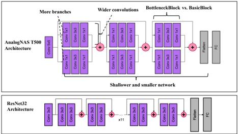<details> <summary>Image 10 Details</summary>  ### Visual Description ## Neural Network Architectures: AnalogNAS T500 vs. ResNet32 ### Overview The image presents a comparison of two neural network architectures: AnalogNAS T500 and ResNet32. It illustrates the structural differences between the two, highlighting aspects such as the number of branches, convolution widths, and overall network depth. ### Components/Axes * **AnalogNAS T500 Architecture:** Depicted in the upper portion of the image. * Components: Conv 5x5, Conv 1x1, Conv 3x3, Addition nodes (+), Flatten, FC (Fully Connected Layer). * Annotations: "More branches", "Wider convolutions", "BottleneckBlock vs. BasicBlock", "Shallower and smaller network". * **ResNet32 Architecture:** Depicted in the lower portion of the image. * Components: Conv 3x3, Addition nodes (+), Flatten, FC (Fully Connected Layer). * Annotation: "x11" indicating a repeating block. ### Detailed Analysis **AnalogNAS T500 Architecture:** * Starts with a Conv 5x5 block. * Splits into two branches, each containing Conv 1x1 and Conv 3x3 blocks. These branches are then added together. * The network then proceeds with wider convolutions, consisting of Conv 1x1 and Conv 3x3 blocks, followed by an addition node. * A "BottleneckBlock vs. BasicBlock" section follows, containing Conv 1x1 and Conv 3x3 blocks, again followed by an addition node. * Finally, the network includes a Flatten layer and a Fully Connected (FC) layer. **ResNet32 Architecture:** * Begins with a Conv 3x3 block. * Repeats a block of Conv 3x3, addition node (+) eleven times (indicated by "x11"). * Concludes with a Flatten layer and a Fully Connected (FC) layer. ### Key Observations * AnalogNAS T500 has more branching and wider convolutions compared to ResNet32. * ResNet32 is a shallower and smaller network, characterized by repeated blocks of Conv 3x3 and addition nodes. * Both architectures end with Flatten and FC layers. ### Interpretation The diagram illustrates the architectural differences between AnalogNAS T500 and ResNet32. AnalogNAS T500 employs a more complex structure with multiple branches and varying convolution sizes, potentially allowing it to capture more intricate features. ResNet32, on the other hand, utilizes a simpler, repetitive structure, which may be more efficient for certain tasks. The "BottleneckBlock vs. BasicBlock" annotation suggests that AnalogNAS T500 may incorporate bottleneck blocks, which are commonly used to reduce computational complexity in deep networks. The "Shallower and smaller network" annotation for ResNet32 indicates that it has fewer layers and parameters compared to AnalogNAS T500. The repetition of the Conv 3x3 block in ResNet32 (x11) is a key characteristic of ResNet architectures, enabling the network to learn hierarchical representations of the input data. </details> A sampled architecture has a widening factor per block. To compute the average widening factor, we first computed the average widening factor per architecture by dividing the sum of the widening factors by the number of blocks contained in the architecture. Then, we calculated the average widening factor across all architectures. Similar computations were performed for the average number of branches. For each plot, the search was run 5 times and the mean is represented in each point. The plotted error corresponds to one standard deviation from that mean. Starting from a random population obtained using LHS, the population evolves through different width and depth-related mutations. During this analysis, we want to answer the following questions: (i) does the search favor wide or deep networks? And subsequently, are wider architectures more noise resilient? (ii) what architectures are exploited by the search for different tasks when constraining the number of parameters? ## A. Are Wider or Deeper Networks More Robust to PCM Device Drift? From Fig. 9, it can be observed that the depth of all networks decreases during the search. This trend is especially seen when we constrain the model's size to 100K and 500K parameters. During the search, the widening factor also increases, allowing the blocks to have wider convolutions. The number of branches is highly dependent on T p . This number is, on average, between 1 and 2. The branches are the number of parallel convolutions in a block disregarding the skip connection. In the literature, architectures such as ResNext, that support a higher number of branches, have a number of parameters around 30M. It is still interesting to get blocks with two branches, which also reflects an increase in the width of the network by increasing the number of features extracted within the same block.The average output channel size of the first convolution decreases during the search. Its final value is around the same number of output channels as standard architectures, i.e., between 16 and 32. This follows the general trend of having wider convolutions in deeper network positions. ## B. Types Of Architectures The architectures and parameter constraints differ for each task, but they all exhibit an increasing expansion ratio in the convolution block. This allows the convolutions to effectively utilize the tile and mitigate noise from unused cells in the crossbar.For CIFAR-10, architectures behave like Wide Resnet [9] while respecting the number of parameters constraint. For the VWW task, the architectures are deeper. The input resolution is 224 × 224 , which requires more feature extraction blocks. However, they are still smaller than SOTA architectures, with a maximum depth of 22. As depth is essential to obtain high accuracy for the VWW task, no additional branches are added. For the KWS task, the architectures are the widest possible, maximizing the tile utilization for each convolutional layer. ## IX. CONCLUSION In this paper, we propose an efficient NAS methodology dedicated to analog in-memory computing for TinyML tasks entitled AnalogNAS. The obtained models are accurate, noise and drift-resilient, and small enough to run on resourceconstrained devices. Experimental results demonstrate that our method outperforms SOTA models on analog hardware for three tasks of the MLPerf benchmark: image classification on CIFAR-10, VWW, and KWS. Our AnalogNAS T500 model implemented on physical hardware demonstrates > 2% higher accuracy experimentally on the CIFAR-10 benchmark than ResNet32. Calculated speed and energy efficiency estimates reveal a > 4 × reduction in execution time, in addition to > 1 . 2 × higher energy efficiency for AnalogNAS T500 compared with ResNet32 when evaluated using a system-level simulator. While our paper has focused on a ResNet-like search space, it is important to note that our search strategy is adaptable and can be extended in future work to explore a broader range of architectures. ## ACKNOWLEDGEMENT We would like to thank Thanos Vasilopoulos and Julian B¨ uchel from IBM Research, Zurich lab, for their help with the development of the hardware-software infrastructure. We also thank the IBM Research Analog AI team for their feedback. We thank the computational support from AiMOS, an AI supercomputer made available by the IBM Research AI Hardware Center and Rensselaer Polytechnic Institute's Center for Computational Innovations (CCI). ## REFERENCES - [1] A. Sebastian, M. Le Gallo, R. Khaddam-Aljameh, and E. Eleftheriou, 'Memory devices and applications for in-memory computing,' Nature Nanotechnology , vol. 15, no. 7, pp. 529-544, Jul 2020. - [2] V. Joshi, M. L. Gallo, I. Boybat, S. Haefeli, C. Piveteau, M. Dazzi, B. Rajendran, A. Sebastian, and E. Eleftheriou, 'Accurate deep neural network inference using computational phase-change memory,' CoRR , vol. abs/1906.03138, 2019. - [3] C. Lammie, W. Xiang, B. Linares-Barranco, and M. Rahimi Azghadi, 'Memtorch: An open-source simulation framework for memristive deep learning systems,' Neurocomputing , vol. 485, pp. 124-133, 2022. - [4] I. Boybat, B. Kersting, S. G. Sarwat, X. Timoneda, R. L. Bruce, M. BrightSky, M. L. Gallo, and A. Sebastian, 'Temperature sensitivity of analog in-memory computing using phase-change memory,' in 2021 IEEE International Electron Devices Meeting (IEDM) , 2021, pp. 28.3.1-28.3.4. - [5] A. G. Howard, M. Zhu, B. Chen, D. Kalenichenko, W. Wang, T. Weyand, M. Andreetto, and H. Adam, 'Mobilenets: Efficient convolutional neural networks for mobile vision applications,' CoRR , vol. abs/1704.04861, 2017. - [6] G. Lu, W. Zhang, and Z. Wang, 'Optimizing depthwise separable convolution operations on gpus,' IEEE Transactions on Parallel and Distributed Systems , vol. 33, no. 1, pp. 70-87, 2022. - [7] H. Benmeziane, K. E. Maghraoui, H. Ouarnoughi, S. Niar, M. Wistuba, and N. Wang, 'A comprehensive survey on hardware-aware neural architecture search,' CoRR , vol. abs/2101.09336, 2021. - [8] S. Xie, R. B. Girshick, P. Doll´ ar, Z. Tu, and K. He, 'Aggregated residual transformations for deep neural networks,' in IEEE Conference on Computer Vision and Pattern Recognition, CVPR . IEEE Computer Society, 2017, pp. 5987-5995. - [9] S. Zagoruyko and N. Komodakis, 'Wide residual networks,' in Proceedings of the British Machine Vision Conference, BMVC , R. C. Wilson, E. R. Hancock, and W. A. P. Smith, Eds. BMVA Press, 2016. - [10] L. Sekanina, 'Neural architecture search and hardware accelerator cosearch: A survey,' IEEE Access , vol. 9, pp. 151 337-151 362, 2021. - [11] C. R. Banbury, V. J. Reddi, P. Torelli, N. Jeffries, C. Kir´ aly, J. Holleman, P. Montino, D. Kanter, P. Warden, D. Pau, U. Thakker, A. Torrini, J. Cordaro, G. D. Guglielmo, J. M. Duarte, H. Tran, N. Tran, W. Niu, and X. Xu, 'Mlperf tiny benchmark,' in Proceedings of the Neural Information Processing Systems Track on Datasets and Benchmarks 1, NeurIPS Datasets and Benchmarks 2021, December 2021, virtual , J. Vanschoren and S. Yeung, Eds., 2021. - [12] C. R. Banbury, C. Zhou, I. Fedorov, R. M. Navarro, U. Thakker, D. Gope, V. J. Reddi, M. Mattina, and P. N. Whatmough, 'Micronets: Neural network architectures for deploying tinyml applications on commodity microcontrollers,' in Proceedings of Machine Learning and Systems , A. Smola, A. Dimakis, and I. Stoica, Eds. mlsys.org, 2021. - [13] H. Liu, K. Simonyan, and Y. Yang, 'DARTS: differentiable architecture search,' CoRR , vol. abs/1806.09055, 2018. [Online]. Available: http://arxiv.org/abs/1806.09055 - [14] E. Liberis, L. Dudziak, and N. D. Lane, ' µ nas: Constrained neural architecture search for microcontrollers,' in EuroMLSys@EuroSys 2021, Proceedings of the 1st Workshop on Machine Learning and Systemsg Virtual Event, Edinburgh, Scotland, UK, 26 April, 2021 , E. Yoneki and P. Patras, Eds. ACM, 2021, pp. 70-79. - [15] G. Li, S. K. Mandal, ¨ U. Y. Ogras, and R. Marculescu, 'FLASH: fast neural architecture search with hardware optimization,' ACM Trans. Embed. Comput. Syst. , vol. 20, no. 5s, pp. 63:1-63:26, 2021. - [16] W. Jiang, Q. Lou, Z. Yan, L. Yang, J. Hu, X. S. Hu, and Y. Shi, 'Device-circuit-architecture co-exploration for computing-in-memory neural accelerators,' IEEE Trans. Computers , vol. 70, no. 4, pp. 595-605, 2021. - [17] Z. Yuan, J. Liu, X. Li, L. Yan, H. Chen, B. Wu, Y. Yang, and G. Sun, 'NAS4RRAM: neural network architecture search for inference on rrambased accelerators,' Sci. China Inf. Sci. , vol. 64, no. 6, 2021. - [18] Z. Yan, D.-C. Juan, X. S. Hu, and Y. Shi, 'Uncertainty modeling of emerging device based computing-in-memory neural accelerators with application to neural architecture search,' in 2021 26th Asia and South Pacific Design Automation Conference (ASP-DAC) , 2021, pp. 859-864. - [19] G. Li, M. Zhang, J. Li, F. Lv, and G. Tong, 'Efficient densely connected convolutional neural networks,' Pattern Recognit. , vol. 109, p. 107610, 2021. - [20] C. Zhou, F. Redondo, J. Buchel, I. Boybat, X. Comas, S. R. Nandakumar, S. Das, A. Sebastian, M. L. Gallo, and P. N. Whatmough, 'Ml-hw codesign of noise-robust tinyml models and always-on analog computein-memory edge accelerator,' IEEE Micro , vol. 42, no. 06, pp. 76-87, 2022. - [21] M. J. Rasch, D. Moreda, T. Gokmen, M. L. Gallo, F. Carta, C. Goldberg, K. E. Maghraoui, A. Sebastian, and V. Narayanan, 'A flexible and fast pytorch toolkit for simulating training and inference on analog crossbar arrays,' in 3rd IEEE International Conference on Artificial Intelligence Circuits and Systems . IEEE, 2021, pp. 1-4. - [22] M. J. Rasch, C. Mackin, M. L. Gallo, A. Chen, A. Fasoli, F. Odermatt, N. Li, S. R. Nandakumar, P. Narayanan, H. Tsai, G. W. Burr, A. Sebastian, and V. Narayanan, 'Hardware-aware training for large-scale and diverse deep learning inference workloads using in-memory computing-based accelerators,' 2023. [Online]. Available: https://arxiv.org/abs/2302.08469 - [23] C. Termritthikun, Y. Jamtsho, J. Ieamsaard, P. Muneesawang, and I. Lee, 'Eeea-net: An early exit evolutionary neural architecture search,' Eng. Appl. Artif. Intell. , vol. 104, p. 104397, 2021. - [24] X. Dai, A. Wan, P. Zhang, B. Wu, Z. He, Z. Wei, K. Chen, Y. Tian, M. Yu, P. Vajda, and J. E. Gonzalez, 'Fbnetv3: Joint architecture-recipe search using predictor pretraining,' in IEEE Conference on Computer Vision and Pattern Recognition, CVPR . Computer Vision Foundation / IEEE, 2021, pp. 16 276-16 285. - [25] W. Jiang, X. Zhang, E. H. Sha, L. Yang, Q. Zhuge, Y. Shi, and J. Hu, 'Accuracy vs. efficiency: Achieving both through fpga-implementation aware neural architecture search,' in Proceedings of the 56th Annual Design Automation Conference 2019, DAC 2019, Las Vegas, NV, USA, June 02-06, 2019 . ACM, 2019, p. 5. - [26] A. Sarah, D. Cummings, S. N. Sridhar, S. Sundaresan, M. Szankin, T. Webb, and J. P. Munoz, 'A hardware-aware system for accelerating deep neural network optimization,' CoRR , vol. abs/2202.12954, 2022. - [27] Z. Dong, Y. Gao, Q. Huang, J. Wawrzynek, H. K. H. So, and K. Keutzer, 'HAO: hardware-aware neural architecture optimization for efficient inference,' in 29th IEEE Annual International Symposium on FieldProgrammable Custom Computing Machines, FCCM 2021, Orlando, FL, USA, May 9-12, 2021 . IEEE, 2021, pp. 50-59. - [28] M. Tan and Q. V. Le, 'Efficientnetv2: Smaller models and faster training,' in Proceedings of the 38th International Conference on Machine Learning, ICML , ser. Proceedings of Machine Learning Research, M. Meila and T. Zhang, Eds., vol. 139. PMLR, 2021, pp. 10 096-10 106. - [29] B. Zoph, V. Vasudevan, J. Shlens, and Q. V. Le, 'Learning transferable architectures for scalable image recognition,' in 2018 IEEE Conference on Computer Vision and Pattern Recognition, CVPR 2018, Salt Lake City, UT, USA, June 18-22, 2018 . Computer Vision Foundation / IEEE Computer Society, 2018, pp. 8697-8710. - [30] K. He, X. Zhang, S. Ren, and J. Sun, 'Deep residual learning for image recognition,' in IEEE Conference on Computer Vision and Pattern Recognition, CVPR . IEEE Computer Society, 2016, pp. 770-778. - [31] M. D. McKay, 'Latin hypercube sampling as a tool in uncertainty analysis of computer models,' in Proceedings of the 24th Winter Simulation Conference, Arlington, VA, USA, December 13-16, 1992 , R. C. Crain, Ed. ACM Press, 1992, pp. 557-564. - [32] X. Ning, Y. Zheng, T. Zhao, Y. Wang, and H. Yang, 'A generic graphbased neural architecture encoding scheme for predictor-based NAS,' in Computer Vision - ECCV 2020 - 16th European Conference, Glasgow, UK, August 23-28, 2020, Proceedings, Part XIII , ser. Lecture Notes in Computer Science, A. Vedaldi, H. Bischof, T. Brox, and J. Frahm, Eds., vol. 12358. Springer, 2020, pp. 189-204. - [33] H. Benmeziane, S. Niar, H. Ouarnoughi, and K. E. Maghraoui, 'Pareto rank surrogate model for hardware-aware neural architecture search,' in International IEEE Symposium on Performance Analysis of Systems and Software, ISPASS . IEEE, 2022, pp. 267-276. - [34] H. Abdi, 'The kendall rank correlation coefficient,' Encyclopedia of Measurement and Statistics. Sage, Thousand Oaks, CA , pp. 508-510, 2007. - [35] A. Krizhevsky, G. Hinton et al. , 'Learning multiple layers of features from tiny images,' 2009. - [36] A. Chowdhery, P. Warden, J. Shlens, A. Howard, and R. Rhodes, 'Visual wake words dataset,' CoRR , vol. abs/1906.05721, 2019. - [37] H. Zhang, C. Wu, Z. Zhang, Y. Zhu, H. Lin, Z. Zhang, Y. Sun, T. He, J. Mueller, R. Manmatha, M. Li, and A. J. Smola, 'Resnest: Splitattention networks,' in IEEE/CVF Conference on Computer Vision and Pattern Recognition Workshops, CVPR . IEEE, 2022, pp. 2735-2745. - [38] M. C. Mukkamala and M. Hein, 'Variants of rmsprop and adagrad with logarithmic regret bounds,' in Proceedings of the 34th International Conference on Machine Learning, ICML , ser. Proceedings of Machine Learning Research, D. Precup and Y. W. Teh, Eds., vol. 70. PMLR, 2017, pp. 2545-2553. - [39] P. Warden, 'Speech Commands: A Dataset for Limited-Vocabulary Speech Recognition,' ArXiv e-prints , Apr. 2018. [Online]. Available: https://arxiv.org/abs/1804.03209 - [40] J. Mart´ ınez, H. P´ erez-Meana, E. E. Hern´ andez, and M. M. Suzuki, 'Speaker recognition using mel frequency cepstral coefficients (MFCC) and vector quantization (VQ) techniques,' in 22nd International Conference on Electrical Communications and Computers, CONIELECOMP , P. B. S´ anchez, R. Rosas-Romero, and M. J. O. Galindo, Eds. IEEE, 2012, pp. 248-251. - [41] D. P. Kingma and J. Ba, 'Adam: A method for stochastic optimization,' in 3rd International Conference on Learning Representations , Y. Bengio and Y. LeCun, Eds., 2015. - [42] J. Lin, W. Chen, Y. Lin, J. Cohn, C. Gan, and S. Han, 'Mcunet: Tiny deep learning on iot devices,' in Advances in Neural Information Processing Systems 33: Annual Conference on Neural Information Processing Systems , H. Larochelle, M. Ranzato, R. Hadsell, M. Balcan, and H. Lin, Eds., 2020. - [43] P. M. Sørensen, B. Epp, and T. May, 'A depthwise separable convolutional neural network for keyword spotting on an embedded system,' EURASIP J. Audio Speech Music. Process. , vol. 2020, no. 1, p. 10, 2020. - [44] M. L. Gallo, R. Khaddam-Aljameh, M. Stanisavljevic, A. Vasilopoulos, B. Kersting, M. Dazzi, G. Karunaratne, M. Braendli, A. Singh, S. M. Mueller, J. Buechel, X. Timoneda, V. Joshi, U. Egger, A. Garofalo, A. Petropoulos, T. Antonakopoulos, K. Brew, S. Choi, I. Ok, T. Philip, V. Chan, C. Silvestre, I. Ahsan, N. Saulnier, V. Narayanan, P. A. Francese, E. Eleftheriou, and A. Sebastian, 'A 64-core mixed-signal in-memory compute chip based on phase-change memory for deep neural network inference,' 2022. [Online]. Available: https://arxiv.org/abs/2212.02872 - [45] R. Khaddam-Aljameh, M. Stanisavljevic, J. F. Mas, G. Karunaratne, M. Braendli, F. Liu, A. Singh, S. M. M¨ uller, U. Egger, A. Petropoulos, T. Antonakopoulos, K. Brew, S. Choi, I. Ok, F. L. Lie, N. Saulnier, V. Chan, I. Ahsan, V. Narayanan, S. R. Nandakumar, M. L. Gallo, P. A. Francese, A. Sebastian, and E. Eleftheriou, 'Hermes core - a 14nm cmos and pcm-based in-memory compute core using an array of 300ps/lsb linearized cco-based adcs and local digital processing,' in 2021 Symposium on VLSI Technology , 2021, pp. 1-2. - [46] S. Jain, H. Tsai, C.-T. Chen, R. Muralidhar, I. Boybat, M. M. Frank, S. Wo´ zniak, M. Stanisavljevic, P. Adusumilli, P. Narayanan, K. Hosokawa, M. Ishii, A. Kumar, V. Narayanan, and G. W. Burr, 'A heterogeneous and programmable compute-in-memory accelerator architecture for analogai using dense 2-d mesh,' IEEE Transactions on Very Large Scale Integration (VLSI) Systems , vol. 31, no. 1, pp. 114-127, 2023.