## In-Context Analogical Reasoning with Pre-Trained Language Models
Xiaoyang Hu 12 ∗
Shane Storks 1 ∗ Richard L. Lewis 2 † Joyce Chai 1 †
1 Computer Science and Engineering Division, University of Michigan 2 Department of Psychology, University of Michigan
{nickhu, sstorks, rickl, chaijy}@umich.edu
## Abstract
Analogical reasoning is a fundamental capacity of human cognition that allows us to reason abstractly about novel situations by relating them to past experiences. While it is thought to be essential for robust reasoning in AI systems, conventional approaches require significant training and/or hard-coding of domain knowledge to be applied to benchmark tasks. Inspired by cognitive science research that has found connections between human language and analogy-making, we explore the use of intuitive language-based abstractions to support analogy in AI systems. Specifically, we apply large pre-trained language models (PLMs) to visual Raven's Progressive Matrices (RPM), a common relational reasoning test. By simply encoding the perceptual features of the problem into language form, we find that PLMs exhibit a striking capacity for zero-shot relational reasoning, exceeding human performance and nearing supervised vision-based methods. We explore different encodings that vary the level of abstraction over task features, finding that higherlevel abstractions further strengthen PLMs' analogical reasoning. Our detailed analysis reveals insights on the role of model complexity, incontext learning, and prior knowledge in solving RPM tasks.
## 1 Introduction
Humans are constantly presented with novel problems and circumstances. Rather than understand them in isolation, we try to connect them with past experiences. With any luck, we might find an analogy : a mapping between relevant aspects of this new situation and a past situation, which helps form abstractions that allow us to reason more effectively in the future (Holyoak, 1984). Analogy is thought to underpin humans' robust reasoning and problem solving capabilities (Hofstadter and
∗ Authors contributed equally to this work.
† Equal advising contribution.
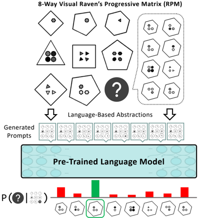
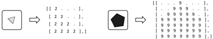
Figure 1: Raven's Progressive Matrices (Raven and Court, 1938; Zhang et al., 2019a) are an analogy-making task where one must infer the missing matrix item based on abstract rules instantiated in the first two rows. To demonstrate the potential analogical reasoning skills in pre-trained language models, we develop languagebased abstractions over their key perceptual features, then prompt them to select the completion of the matrix.
<details>
<summary>Image 1 Details</summary>
### Visual Description
\n
## Diagram: 8-Way Visual Raven's Progressive Matrix (RPM) Process
### Overview
The image depicts a diagram illustrating the process of solving an 8-Way Visual Raven's Progressive Matrix (RPM) using a pre-trained language model. The process involves generating language-based abstractions from the visual matrix and then using these abstractions to predict the missing element. The diagram shows the input RPM, the generated prompts, the language model, and the probability distribution over possible answers.
### Components/Axes
The diagram is structured into four main sections:
1. **8-Way Visual Raven's Progressive Matrix (RPM):** A 3x3 grid of shapes with one missing element, marked with a question mark.
2. **Language-Based Abstractions:** A row of small grids representing the generated prompts from the RPM.
3. **Pre-Trained Language Model:** A large, light-blue rectangular block representing the language model. It is depicted as a network of interconnected nodes.
4. **Probability Distribution:** A bar chart showing the probability of each possible answer being the correct one. The x-axis represents the possible answers (each depicted as a small RPM element), and the y-axis represents the probability P(? | …).
### Detailed Analysis or Content Details
**1. 8-Way Visual Raven's Progressive Matrix (RPM):**
The RPM consists of 8 shapes (a diamond, hexagon, triangle, square, and variations of these) arranged in a 3x3 grid with the bottom-right cell missing. The shapes contain varying numbers of filled circles.
**2. Language-Based Abstractions:**
Below the RPM, there is a row of 8 small grids, each representing a language-based abstraction of one of the RPM elements. These abstractions appear to be visual representations of the shapes and their features.
**3. Pre-Trained Language Model:**
The language model is a large, light-blue rectangle with a network of interconnected nodes inside. This visually represents the complexity of the model.
**4. Probability Distribution:**
The bar chart at the bottom shows the probability distribution over the possible answers. The x-axis displays the 8 possible answer choices, each represented by a small RPM element. The y-axis is labeled "P(? | …)", representing the probability of each answer being the correct one given the context.
- The first 7 bars are red and relatively short, indicating low probability.
- The 8th bar is green and significantly taller, indicating a high probability.
- The height of the red bars is approximately 0.1-0.2 (estimated).
- The height of the green bar is approximately 0.6-0.8 (estimated).
### Key Observations
- The language model assigns a significantly higher probability to one of the possible answers compared to the others.
- The visual representation of the language model suggests a complex network.
- The diagram illustrates a pipeline from visual input (RPM) to language abstraction to probabilistic prediction.
### Interpretation
This diagram demonstrates a method for solving visual reasoning problems (like RPMs) using a pre-trained language model. The process involves translating the visual information into a language-based representation that the model can understand and reason about. The model then uses this representation to predict the missing element in the RPM, outputting a probability distribution over the possible answers. The high probability assigned to one answer suggests that the model has successfully identified the underlying pattern in the RPM. The use of a pre-trained language model indicates that the model leverages prior knowledge to solve the problem, rather than learning from scratch. This approach highlights the potential of combining visual and linguistic reasoning for solving complex cognitive tasks. The diagram is a conceptual illustration of the process, rather than a presentation of specific data or results. It is a visual explanation of a methodology.
</details>
Sander, 2013), and thus it is believed to be prerequisite in order to enable the same in AI systems. However, conventional approaches struggle with analogy-making, and are trained on thousands of examples to achieve any success on benchmark tasks. This is unsatisfying, as humans are capable of analogy-making without explicit training, and such analogy-making should enable zero-shot generalization to new situations (Mitchell, 2021).
Interestingly, a body of work in cognitive science suggests that analogy-making and relational reasoning are connected to humans' symbol system and language capabilities (Gentner, 2010). For example, Gordon (2004) finds that members of an Amazonian tribe that count only with words for 'one,' 'two,' and 'many' struggle to make analo- gies with higher numbers. Further, Gentner et al. (2013) find that deaf children whose sign language does not involve spatial relations are outperformed by hearing children on a spatial relational reasoning task, while Christie and Gentner (2014) find that assigning even nonsensical names to relations enhances children's relational reasoning. All of this demonstrates that language serves as a powerful way for humans to abstract and better reason about the overwhelming and complex percepts we encounter in the world.
In this work, we explore whether language may serve a similar purpose in AI systems. Specifically, we apply contemporary autoregressive pre-trained language models (PLMs) to Raven's Progressive Matrices (RPM), an example of which is shown in Figure 1. RPM is a widely used psychometric test for relational reasoning that requires inducing an abstract rule from just two examples of short sequences of groups of shapes, and then applying the rule to complete a new partial sequence (Raven and Court, 1938). This task makes minimal assumptions about the test taker's prior knowledge, and is thus thought to provide a good estimate for general intelligence (Holyoak, 2012). On the RAVEN dataset (Zhang et al., 2019a), we find that given the ability to perceive key features of RPMs, large PLMs exhibit a surprising capacity for zero-shot relational reasoning, approaching that of supervised vision-based deep learning approaches and even humans. We propose three levels of abstraction over the language features of the task using name assignment and task decomposition, and find that each abstraction further strengthens PLMs' relational reasoning. Our results and detailed analysis offer insights on PLM performance, including the role of models' complexity, in-context learning, and prior knowledge in emergent relational reasoning, and suggest that they could play an important role in future cognitive architectures for analogy-making. 2
## 2 Related Work
Past work has studied analogy in AI across various domains. Mitchell (2021) provides a comprehensive overview of these efforts, especially those applied in idealized symbolic domains. Here, symbolic and probabilistic methods have traditionally been applied (Gentner, 1983; Hofstadter and Mitchell, 1994; Lake et al., 2015). However, these
2 Experiment code is available at https://github.com/ hxiaoyang/lm-raven.
approaches typically require hard-coding domainspecific concepts, and require substantial search through domain knowledge to operate on their target problems, thus making them unscalable. The creation of large-scale image datasets for analogy tasks here (Zhang et al., 2019a; Hu et al., 2021; Odouard and Mitchell, 2022) have enabled further research with deep learning and neuro-symbolic methods (Hill et al., 2019; Spratley et al., 2020; Kim et al., 2020; Zhang et al., 2021), which bring the advantage of requiring less ad-hoc encoding of domain knowledge, but require thousands of training examples to learn the tasks, still limiting their generalization capability.
Other work has explored AI systems' analogymaking in real-world domains, including in natural images (Teney et al., 2020; Bitton et al., 2022) and language (Li et al., 2020; Chen et al., 2022; Sultan and Shahaf, 2022), especially lexical analogies (Turney et al., 2003; Turney, 2008; Speer et al., 2008; Mikolov et al., 2013b,a; Linzen, 2016; Lu et al., 2019). However, these domains make it difficult to control the prior knowledge required to solve tasks (Mitchell, 2021), and in the context of recent generative foundation models that are extensively pre-trained on natural data, it becomes difficult to separate analogy learning from distributional patterns that can be overfit. Unlike prior work, we apply such foundation models for language to analogical reasoning in a zero-shot setting, bypassing the requirement of hard-coding domain knowledge or training models on task-specific data. Furthermore, while contemporaneous work has applied PLMs to a variety of simpler relational reasoning tasks in language (Webb et al., 2022), we systematically explore the advantage of using language to abstract over complex visual features of the task, opening questions about how the powerful symbol systems learned in PLMs may support robust, perception-driven reasoning in future AI systems.
## 3 Raven's Progressive Matrices
Raven's progressive matrices (RPM) are abstract relational reasoning tasks used in cognitive psychology to test humans' analogy-making (Raven and Court, 1938). Each instance of RPM is a matrix consisting of 9 items arranged in a square, the last of which must be selected from a set of choices. Each item consists of several perceptual attributes , such as shape, color, or more abstract features. Within each row of the matrix, a relation is applied
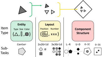
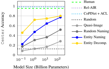
Figure 2: Illustration of the compositional nature of entities, layouts, and component structures in RA VEN, and their unique attributes. We provide example items from sub-tasks each item type appears in.
<details>
<summary>Image 2 Details</summary>
### Visual Description
\n
## Diagram: Visual Representation of Item Manipulation
### Overview
The image is a diagram illustrating a process of item manipulation, breaking it down into three main aspects: Item Type, Layout, and Component Structure. It shows a flow from a single item to multiple items, and then to a complex item, with sub-tasks associated with each aspect. The diagram uses shapes and arrows to represent the process and its components.
### Components/Axes
The diagram is divided into three main sections, each enclosed in a rounded rectangle:
* **Item Type** (Green): This section focuses on the characteristics of the item, with labels for "Type", "Size", and "Color". Example shapes are provided: triangle, line, circle, and square.
* **Layout** (Yellow): This section deals with the arrangement of items, with labels for "Position" and "Number". It shows examples of 2x2 and 3x3 grids.
* **Component Structure** (Pink): This section focuses on the internal structure of the item, with labels for L-R, U-D, O-IC, and O-IG.
* **Flow Arrows**: A green arrow originates from the single triangle and points to a set of three smaller shapes (triangle, inverted triangle, triangle). A yellow arrow originates from the set of three shapes and points to a complex shape containing smaller triangles.
* **Sub-Tasks**: Below each section are examples of sub-tasks represented by different shapes: hexagon (Center), diamond and circle (2x2Grid, 3x3Grid), pentagon and circle (L-R, U-D), pentagon and square (O-IC, O-IG).
### Detailed Analysis or Content Details
* **Item Type:**
* **Type:** The diagram shows four item types: triangle, line, circle, and square.
* **Size:** The diagram implies size variation, as the initial triangle is larger than the triangles within the complex shape.
* **Color:** The diagram uses black for all shapes.
* **Layout:**
* **Position:** The diagram shows a grid-like arrangement with "X" marks indicating positions.
* **Number:** The diagram shows "XXX" representing the number of items in a layout.
* **2x2 Grid:** Contains a diamond and a square.
* **3x3 Grid:** Contains nine circles.
* **Component Structure:**
* **L-R:** A pentagon and a circle.
* **U-D:** A diamond and a circle.
* **O-IC:** A pentagon and a square.
* **O-IG:** A square.
* **Flow:**
* A single dark gray triangle is transformed into three smaller triangles (dark gray, inverted dark gray, dark gray).
* These three triangles are then combined into a more complex shape containing smaller triangles.
* **Sub-Tasks:**
* **Center:** Hexagon.
* **2x2Grid:** Diamond and Square.
* **3x3Grid:** Nine Circles.
* **L-R:** Pentagon and Circle.
* **U-D:** Diamond and Circle.
* **O-IC:** Pentagon and Square.
* **O-IG:** Square.
### Key Observations
* The diagram illustrates a hierarchical process of item manipulation, starting with a single item and progressing to more complex arrangements.
* The "Layout" section suggests the arrangement of items within a defined space.
* The "Component Structure" section indicates the internal organization of the item.
* The sub-tasks provide examples of how each aspect can be implemented.
### Interpretation
The diagram likely represents a conceptual model for visual reasoning or object manipulation in a computational context. It suggests a process where an initial item (triangle) undergoes transformations in terms of its type, layout, and internal structure. The flow arrows indicate a sequential process, where the output of one stage becomes the input for the next. The sub-tasks provide concrete examples of how these transformations can be achieved.
The diagram could be used to explain how a system might decompose a complex object into its constituent parts, arrange those parts in a specific layout, and then combine them to create a new object. The labels "L-R", "U-D", "O-IC", and "O-IG" might refer to specific operations or relationships within the component structure, such as left-to-right, up-down, inside-center, and inside-grid.
The diagram is abstract and does not provide specific numerical data. However, it offers a valuable visual representation of a complex process, highlighting the key components and their relationships. It is a conceptual illustration rather than a data-driven chart.
</details>
over these attributes, such as progression of numerical values associated with these attributes. Given the first two rows of the matrix, the challenge of the task is to identify the relations being applied to items, and apply them analogously in the third row to infer the missing ninth item. Successfully solving an RPM requires tackling two sub-problems: perception of each item's attributes, and reasoning over multiple items' attributes to infer and apply relations.
## 3.1 RAVEN Dataset
We focus our study on RAVEN (Zhang et al., 2019a), which provides a large-scale benchmark for RPM tasks for training and evaluation of AI systems. Each RPM has 8 possible candidate items to complete it. As shown in Figure 2, each item may consist of compositional entities , layouts , and/or component structures , and RAVEN provides a suite of increasingly complex sub-tasks built from these elements. We introduce their unique attributes below, as well as relations that may occur over them across items in the matrix.
Entities. A single entity has a type (i.e., shape), size , and color selected from a small number of classes. Each of these attributes is associated with a number: type with the number of sides in the entity's shape, size with its diameter, and color with the darkness of its shading. The simplest sub-task of RAVEN is Center , where each item only consists of a single entity.
Layouts. Layouts of entities bring additional higher-level attributes to items, specifically the number (i.e., count) and position of entities within a layout. In the 2x2Grid and 3x3Grid sub-tasks of RAVEN, each item consists of multiple entities arranged in a grid.
Component structures. Items may also be composed of multiple sub-items or components ; RAVEN includes four sub-tasks that introduce this even higher-level challenge: L-R , U-D , and O-IC , each of which consist of two single entities in different configurations, and O-IG , which consists of a 2-by-2 grid inside of a larger entity.
Relations. Following prior work on this task, RAVEN applies four different relations to item attributes across rows of the matrix. These are Constant , which does not modify an attribute, Progression , which increases or decreases the value of an attribute by 1 or 2, Arithmetic , which performs addition or subtraction on the first two attributes of the row to create the third, and Distribute Three , which distributes three consistent values of an attribute across each row.
## 4 Methods
In order to apply PLMs to RAVEN, we abstract the visual features of the task into language. Our abstractions are intentionally applied on a per-item basis to tackle the perception problem of the task without giving the PLM explicit hints toward the reasoning problem (which requires capturing patterns over multiple items). This allows us to focus on evaluating the reasoning capabilities of PLMs. 3
First, we introduce our multi-level abstractions for the RAVEN dataset. 4 Then we formally define the interface between PLMs and the RPM task.
## 4.1 Abstractions in RAVEN
We define abstractions for entity-level attributes, layout-level attributes, and component structures which convert the RPM task into one or more text prompts. We apply two kinds of abstractions: naming and decomposition . As discussed in Section 1, assigning names to perceptual features strengthens humans' analogy-making skills over them. Inspired by this, naming abstractions abstract over attributes or combinations of attributes in the RPM by assigning a unique name to describe them. Mean-
3 As the important features of RAVEN are simple, the perception of an individual item is better performed by computer vision models, and can already be done to fairly high accuracy (Zhang et al., 2021). For more general-purpose analogymaking beyond idealized domains, the robust perception of key features that allow previous (source) experiences to be mapped to novel (target) experiences is a challenging unsolved problem (Mitchell, 2021).
4 Some example PLM prompts using these abstractions are shown in this section, while more examples are provided in Appendix C.
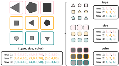
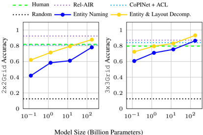
Figure 3: Example generated prompts for a complete RPM under entity attribute naming (left) and decomposition (right) abstractions in the Center sub-task.
<details>
<summary>Image 3 Details</summary>
### Visual Description
\n
## Diagram: Shape Attribute Decomposition
### Overview
The image presents a diagram illustrating the decomposition of a set of shapes based on three attributes: type, size, and color. A 3x3 grid of shapes is shown on the left, with corresponding attribute representations on the right, organized into "type", "size", and "color" categories. The attributes are represented numerically in a table at the bottom.
### Components/Axes
The diagram is divided into four main sections:
1. **Shape Grid:** A 3x3 grid containing nine shapes, each enclosed in a colored box.
2. **Type Legend:** A grid of shape outlines representing different types (triangle, pentagon, square).
3. **Size Legend:** A grid of circles with varying sizes, representing different size categories.
4. **Color Legend:** A grid of colored squares representing different color shades.
5. **Attribute Table:** A table listing the (type, size, color) values for each shape in the grid.
The axes are implicit, defined by the rows and columns of the grids and the table. The legends provide the mapping between visual elements and numerical values.
### Detailed Analysis or Content Details
**Shape Grid:**
The shapes are arranged in a 3x3 grid. Each shape is enclosed in a colored border.
- Row 1: Triangle (pink), Pentagon (yellow), Square (gray)
- Row 2: Square (orange), Triangle (yellow), Pentagon (teal)
- Row 3: Pentagon (teal), Square (gray), Triangle (blue)
**Type Legend:**
The legend shows three shape types:
- Triangle: Represented by the symbol "△"
- Pentagon: Represented by the symbol "☆"
- Square: Represented by the symbol "□"
The legend is organized into a 3x3 grid with the following values:
- Row 1: 3, 5, .
- Row 2: 4, 3, 4
- Row 3: 5, 4, 3
**Size Legend:**
The legend shows three size categories, represented by circles of different sizes.
- Small: Represented by a small circle "●"
- Medium: Represented by a medium circle "●"
- Large: Represented by a large circle "●"
The legend is organized into a 3x3 grid with the following values:
- Row 1: 8, 8, 8
- Row 2: 4, 4, 4
- Row 3: 3, 3, 3
**Color Legend:**
The legend shows three color shades, represented by colored squares.
- Light Gray: Represented by a light gray square.
- Medium Gray: Represented by a medium gray square.
- Dark Gray: Represented by a dark gray square.
The legend is organized into a 3x3 grid with the following values:
- Row 1: 6, 7, 8
- Row 2: 6, 7, 8
- Row 3: 4, 5, 6
**Attribute Table:**
The table lists the (type, size, color) values for each shape in the grid. The values are represented as tuples.
- Row 1: (3.0, 8.60), (5.0, 8.70), (4.0, 8.80)
- Row 2: (4.0, 5.30), (3.0, 4.70), (5.0, 4.80)
- Row 3: (5.0, 3.40), (4.0, 3.50), (3.0, 3.60)
### Key Observations
- Each shape in the grid is uniquely defined by its type, size, and color.
- The attribute table provides a numerical representation of these attributes.
- The legends provide a mapping between visual elements and numerical values.
- The values in the attribute table appear to be floating-point numbers, suggesting a continuous or fine-grained representation of the attributes.
### Interpretation
The diagram demonstrates a method for representing complex objects (shapes) using a set of attributes. The decomposition into type, size, and color allows for a structured and quantifiable description of each shape. The numerical representation in the attribute table facilitates data analysis and comparison. The legends serve as a key to translate between visual and numerical representations.
The diagram suggests a system for categorizing and classifying shapes based on their inherent properties. This could be used in various applications, such as image recognition, object detection, or data visualization. The use of numerical values for attributes allows for more precise and nuanced descriptions than simple categorical labels. The arrangement of the shapes and attributes in a grid format provides a clear and organized visual representation of the data.
</details>
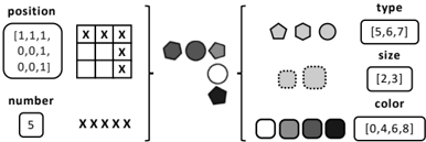
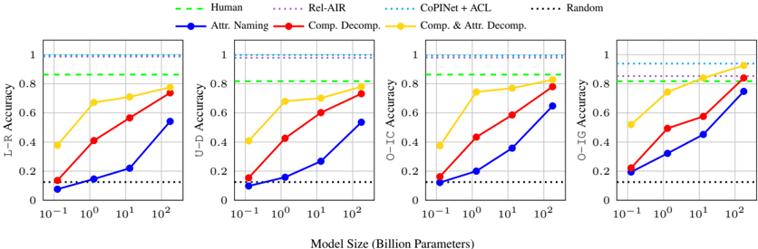
Figure 4: Example of generated entity layout encodings when abstracting position and number , and summarizing redundant entity attributes within the layout.
<details>
<summary>Image 4 Details</summary>
### Visual Description
\n
## Diagram: Visual Representation of Object Attributes
### Overview
The image presents a diagram illustrating the attributes of a set of objects. These attributes are position, number, type, size, and color. The diagram uses a combination of a grid, symbols, and labeled boxes to represent these attributes. It appears to be a visual encoding of data, potentially for a dataset of objects.
### Components/Axes
The diagram is divided into four main sections, arranged horizontally.
* **Position:** A 3x3 grid with "X" marks indicating object locations. The coordinates are labeled as [1,1,1], [0,0,1], [0,0,11].
* **Number:** A box containing the number "5" and five "X" symbols.
* **Type:** A set of shapes (pentagons and circles) with the label "type" and the range [5,6,7].
* **Size:** A set of shapes (solid and dotted circles) with the label "size" and the range [2,3].
* **Color:** A set of filled circles with varying shades of gray and black, labeled "color" and the range [0,4,6,8].
### Detailed Analysis or Content Details
**Position:**
The grid shows "X" marks at the following coordinates: (0,0), (0,1), (0,2), (1,0), (1,2). The grid is labeled with coordinates [1,1,1], [0,0,1], [0,0,11] at the top left.
**Number:**
There are 5 "X" symbols, corresponding to the number "5" in the box.
**Type:**
There are three distinct shapes representing types:
* Pentagon (appears twice)
* Solid Circle (appears once)
* Dotted Circle (appears once)
The type range is [5,6,7].
**Size:**
There are two distinct shapes representing sizes:
* Solid Circle (size 2)
* Dotted Circle (size 3)
The size range is [2,3].
**Color:**
There are four distinct shades of gray and black representing colors:
* White (color 0)
* Light Gray (color 4)
* Medium Gray (color 6)
* Black (color 8)
The color range is [0,4,6,8].
The objects are visually represented as follows:
* A dark gray pentagon.
* A medium gray pentagon.
* A light gray circle.
* A black pentagon.
* A white dotted circle.
* A light gray dotted circle.
### Key Observations
The diagram presents a clear mapping between visual attributes (shape, color, size) and numerical values. The "position" attribute is represented by a grid, while the other attributes are represented by variations in shape, size, and color. The number of objects is explicitly stated as 5.
### Interpretation
The diagram appears to be a visual encoding of a dataset containing 5 objects. Each object is characterized by its position, type, size, and color. The diagram allows for a quick visual assessment of the distribution of these attributes across the dataset. The use of different shapes and colors suggests that these attributes are categorical or discrete. The ranges provided for type, size, and color indicate the possible values these attributes can take. The diagram could be used for data exploration, visualization, or communication of data characteristics. The grid representation of position suggests a spatial component to the data.
</details>
while, jointly understanding and tracking the complex features of the task can become a burden even for humans. Inspired by humans' capability to decompose complex tasks into independent subtasks (Lee and Anderson, 2001), decomposition abstractions split the RPM into multiple sub-matrices by its independent features, then generate a separate prompt for each one. We can then prompt a PLMonce for each sub-matrix, and aggregate PLM outputs to choose a candidate matrix completion. 5
## 4.1.1 Entity-Level Abstractions
As shown in Figure 3, we can abstract perceptual entity attributes into language by assigning them names, then generating prompts to represent the full RPM using these names. As each of an entity's attributes is numerical by nature, we assign each attribute an ordinal numerical name; type is named by the number of sides of the associated shape (e.g., '3' for triangle ), size is named by a decimal representing its diameter, and color is named based on the darkness of the entity's shade. As each of an entity's attributes is independent, i.e., a relation over one attribute has no connection to relations over other attributes, we can decompose the RPM task by these attributes into three separate sub-tasks with their own prompts.
5 A more formal definition for decomposition is provided in Section 4.2.
## 4.1.2 Layout-Level Abstractions
As shown in Figure 4, we next propose abstractions for layouts of entities (e.g., in grid-based sub-tasks of RAVEN). First, the number attribute of a layout corresponds to the count of entities in it. Recognizing number requires implicitly counting entities within a layout, which may be difficult to disentangle from other attributes. As such, we directly expose this attribute by extracting this count and encoding it in text. Since this layout attribute is independent from other attributes, we can again decompose the task and consider it separately from entity attributes.
The position attribute encodes even more complex information about a layout, and relations over it may move entities around within the layout. However, an occupancy map serves as a strong naming abstraction for position which omits distracting details of specific entities while exposing key information for detecting relations over it. We generate the occupancy map as an array of text representing the occupancy of the layout, and decompose this from other attributes. Notably, this abstraction provides a unique language description for each possible global configuration of entities within a layout, allowing the PLM to disentangle global and local patterns in the problem, a helpful capability of humans (Robertson and Lamb, 1991). 6
In RAVEN, relations are applied to specific attributes consistently across all entities in a layout. As our layout-level abstractions make explicit the key features of layouts, we no longer need to track entity-level attributes for specific entities within them. Specifically, rather than supply a PLM with a separate grid-like prompt for each entity-level attribute, we simply provide a list of unique attribute values. This reduces the complexity added by layouts of multiple entities.
## 4.1.3 Structural Decomposition Abstractions
In cases with multiple components in each item, we may find that prompts become long and complicated with earlier approaches. Since each component's attributes and relations are independent, we can alternatively decompose the task by its components. For each component, we can generate a prompt through entity attribute naming abstractions as shown in Figure 3 (left), or we can apply
6 For example, we may recognize the grid of entities in Figure 2 to be in an 'L' shape at the global level, while also recognizing that it is locally composed of triangles.
the higher-level abstractions over entity and layout attributes shown in Figure 4, thus decomposing each component's prompts into prompts for each attribute. As this structural decomposition converts multi-component problems into several simpler single-component, single-attribute problems, the complexity added by multiple components is abstracted away.
## 4.2 Problem Definition
Formally, a complete RPM M consists of 9 matrix items m ij where row and column i, j ∈ { 1 , 2 , 3 } . As discussed in Section 3.1, an individual item m ij in the RAVEN dataset is formalized by high-level components consisting of layout-level attributes and entity-level attributes. Given all items in M except for m 33 , the task is to identify m 33 from a set Y of 8 choices by identifying abstract rules over the attributes within the first 2 rows of M , and selecting the candidate m 33 that correctly applies these rules in the third row.
Applying PLMs. We apply PLMs to RAVEN in a zero-shot setting. In the absence of decomposition abstractions, we define ▲ as the mapping of a complete RPM to a text prompt. The PLM's choice for m 33 is given by
$$\arg \max _ { y \in Y } \frac { 1 } { | \mathbb { L } | } \log \Pr \left ( \mathbb { L } \left ( m _ { 1 1 \colon 3 2 } , y \right ) \right )$$
▲ where | ▲ | denotes the number of tokens in the prompt. When decomposition is introduced, ▲ instead returns multiple prompts, and the (tokenlength normalized) log-probabilities of all subprompts are summed. 7
## 5 Experimental Results
Now, we can examine the impact each of these language-based abstractions has on the performance of transformer-based, autoregressive PLMs in relational reasoning on RAVEN. To further understand their impact with respect to model complexity, we evaluate a range of model sizes: 8 OPT 125M, 1.3B, and 13B (Zhang et al., 2022), along with GPT-3 (Brown et al., 2020). 9 Models are evaluated on a random subset of 500 testing examples from each sub-task of RAVEN.
7 See Appendix C for examples of decomposing prompts.
8 Results on additional model sizes in Appendix A.
9 Specifically, we use the text-davinci-002 variant of InstructGPT (Ouyang et al., 2022) through a Microsoft Azure OpenAI deployment.
After introducing some comparison approaches, we present the experimental results from our applied abstractions on PLMs' entity-level, layoutlevel, and component-level relational reasoning. Afterward, we dive deeper with an analysis on how both our abstractions and in-context learning contribute to model performance.
## 5.1 Comparison Approaches
To contextualize our findings, we provide results from the human study in Zhang et al. (2019a), as well as two supervised baselines from prior work. 10 Additionally, to specifically evaluate the advantage of the way we mapped the RPM task into language, we include two simpler abstraction methods that encode task information less explicitly.
Supervised baselines. While our goal is not to achieve the state of the art on RA VEN, we include results from two state-of-the-art supervised baselines for reference. Specifically, we select the two approaches with the top mean accuracy on RAVEN, as outlined in the survey by Małki´ nski and Ma´ ndziuk (2022): Rel-AIR (Spratley et al., 2020) and CoPINet + ACL (Kim et al., 2020). Rel-AIR combines a simple vision model with an unsupervised scene decomposition module, enabling more generalizable reasoning over entities in RAVEN. CoPINet + ACL applies an analogy-centric contrastive learning paradigm to CoPINet (Zhang et al., 2019b), a prior architecture proposed for perceptual inference trained through contrastive learning. Both baselines have been trained on thousands of examples from the RAVEN dataset, and incorporate task-specific inductive biases in their architecture. Meanwhile, we evaluate PLMs on RAVEN in a zero-shot setting with no supervised learning.
Quasi-image abstraction. To evaluate the helpfulness of naming abstractions over entity attributes, we should compare to an approach that does not have such abstraction. However, some mapping from the visual features of the RPM task into langauge is needed in order for a PLM to interface with it. While the limited context window of PLMs restricts us from incorporating raw pixels directly into our prompts, PLMs have recently been demonstrated to capture spatial patterns in similar inputs: text-based matrices (Patel and Pavlick,
10 Since our approach is not evaluated on the exact same subset of RAVEN data, these results from prior work are not directly comparable, but can be helpful reference points.
Figure 5: Quasi-image abstractions for a triangle and pentagon of different size and color .
<details>
<summary>Image 5 Details</summary>
### Visual Description
\n
## Diagram: Shape to Matrix Transformation
### Overview
The image depicts a visual transformation process. It shows two distinct stages: a triangle shape being transformed into a 5x5 matrix of numerical values, and a pentagon shape being transformed into another 5x5 matrix of numerical values. Each transformation is indicated by an arrow.
### Components/Axes
There are no explicit axes or legends. The components are:
1. A triangle within a square frame.
2. A 5x5 matrix of numbers following the triangle.
3. A pentagon within a square frame.
4. A 5x5 matrix of numbers following the pentagon.
5. Arrows indicating the transformation direction.
### Detailed Analysis or Content Details
**Transformation 1: Triangle to Matrix**
The matrix associated with the triangle is:
```
[ [1, 2, ., ., 1],
[2, 2, ., ., 1],
[2, 2, 2, ., 1],
[2, 2, 2, 2, 1],
[2, 2, 2, 2, 1] ]
```
**Transformation 2: Pentagon to Matrix**
The matrix associated with the pentagon is:
```
[ [., ., 9, ., .],
[., 9, 9, 9, .],
[9, 9, 9, 9, 9],
[9, 9, 9, 9, 9],
[9, 9, 9, 9, 9] ]
```
### Key Observations
* The values in the matrices are primarily integers.
* The first matrix contains mostly '1' and '2' values, with some '.' placeholders.
* The second matrix contains mostly '9' values, with some '.' placeholders.
* The '.' character appears to represent a missing or undefined value.
* The matrices are square, with dimensions 5x5.
* The values seem to increase as you move down and to the right in both matrices.
### Interpretation
The diagram illustrates a mapping from geometric shapes (triangle and pentagon) to numerical matrices. The specific rule governing this mapping is not explicitly stated, but it appears to be a function that assigns numerical values based on the shape's characteristics or position within the square frame. The increasing values within the matrices might represent some form of density or intensity related to the shape. The use of '.' suggests that the mapping is not complete or that certain positions are not influenced by the shape.
The transformation could represent a process of discretization or quantization, where a continuous geometric form is converted into a discrete numerical representation. It could also be a simplified model of image processing or pattern recognition, where shapes are encoded as numerical data for further analysis. Without additional context, the precise meaning of the transformation remains ambiguous. The change in values from the first matrix to the second suggests a different mapping function or a different shape influencing the matrix values.
</details>
Figure 6: Results on the RAVEN Center sub-task under entity abstractions, compared to naïve and supervised baselines described in Section 5.1, and humans.
<details>
<summary>Image 6 Details</summary>
### Visual Description
## Line Chart: Center Accuracy vs. Model Size
### Overview
This image presents a line chart illustrating the relationship between "Center Accuracy" and "Model Size (Billion Parameters)" for various methods. The chart compares the performance of different approaches, including human performance, several automated methods, and random baselines.
### Components/Axes
* **X-axis:** "Model Size (Billion Parameters)" with markers at 10<sup>-1</sup>, 10<sup>0</sup>, 10<sup>1</sup>, and 10<sup>2</sup>.
* **Y-axis:** "Center Accuracy" ranging from 0 to 1.
* **Legend (top-right):**
* Human (green, dashed)
* Rel-AIR (black, dotted)
* CoPINet + ACL (cyan, dashed-dotted)
* Random (black, dotted)
* Quasi-Image (gray, solid)
* Random Naming (dark gray, solid)
* Entity Naming (blue, solid)
* Entity Decomp. (yellow, solid)
### Detailed Analysis
The chart displays several lines representing the performance of each method as model size increases.
* **Human:** The green dashed line remains consistently at a Center Accuracy of approximately 1.0 across all model sizes.
* **Rel-AIR:** The black dotted line starts at approximately 0.1 and remains relatively flat, fluctuating around 0.15-0.2 across all model sizes.
* **CoPINet + ACL:** The cyan dashed-dotted line starts at approximately 0.2 and increases to around 0.35 at a model size of 10<sup>1</sup>, then plateaus.
* **Random:** The black dotted line starts at approximately 0.1 and remains relatively flat, fluctuating around 0.15-0.2 across all model sizes.
* **Quasi-Image:** The gray solid line starts at approximately 0.2 and increases to around 0.55 at a model size of 10<sup>1</sup>, then continues to approximately 0.6 at a model size of 10<sup>2</sup>.
* **Random Naming:** The dark gray solid line starts at approximately 0.2 and increases to around 0.4 at a model size of 10<sup>1</sup>, then continues to approximately 0.5 at a model size of 10<sup>2</sup>.
* **Entity Naming:** The blue solid line starts at approximately 0.2 and increases sharply to around 0.65 at a model size of 10<sup>1</sup>, then continues to approximately 0.8 at a model size of 10<sup>2</sup>.
* **Entity Decomp.:** The yellow solid line starts at approximately 0.2 and increases sharply to around 0.75 at a model size of 10<sup>1</sup>, then continues to approximately 0.8 at a model size of 10<sup>2</sup>.
### Key Observations
* Human performance consistently achieves perfect accuracy (1.0).
* The "Entity Naming" and "Entity Decomp." methods show the most significant improvement in Center Accuracy as model size increases.
* "Rel-AIR" and "Random" methods exhibit minimal improvement with increasing model size, remaining near a baseline accuracy of approximately 0.1-0.2.
* "CoPINet + ACL" shows moderate improvement, plateauing at a lower accuracy than "Entity Naming" and "Entity Decomp."
* "Quasi-Image" and "Random Naming" show moderate improvement, but remain below the performance of "Entity Naming" and "Entity Decomp."
### Interpretation
The data suggests that increasing model size significantly improves the performance of "Entity Naming" and "Entity Decomp." methods in terms of Center Accuracy. These methods outperform the other approaches, particularly as the model size grows. The relatively flat performance of "Rel-AIR" and "Random" indicates that these methods do not benefit substantially from larger models. The consistent high accuracy of human performance serves as an upper bound for the automated methods. The chart demonstrates a clear correlation between model size and performance for certain approaches, highlighting the potential benefits of scaling up models for tasks involving entity recognition or decomposition. The plateauing of "CoPINet + ACL" suggests that its performance may be limited by factors other than model size. The difference between "Entity Naming" and "Entity Decomp." is minimal, suggesting they are similarly effective.
</details>
2021). As such, we propose a quasi-image abstraction which converts the visual RPM task into a matrix of ASCII characters. As shown in Figure 5, an entity's type can be expressed through a matrix of characters; size can be expressed through the height and width of the matrix; and color can be expressed through the actual characters making up the matrix. By converting instances of RAVEN's Center sub-task into this pixel-like form, we have a lower-level abstraction of the task's visual features that can be compared to the higher-level abstraction of naming entity attributes.
Random naming abstraction. We would also like to understand the advantage of the specific names we chose for entity attributes compared to other possible choices. As such, we propose a second baseline where, instead of using ordinal labels to describe entities' type , size , and color , we choose random words from a large corpus. This removes numerical dependencies that may be utilized to recognize some relations, and can help us understand whether PLMs take advantage of this information when it is available.
## 5.2 Entity-Level Reasoning
We first evaluate PLMs under our lowest level abstractions over entity attributes. To isolate the improvements from such abstraction, we focus on the Center sub-task of RAVEN which only includes a single entity per item in the RPM, and thus only tests understanding of relations over entity attributes. The results are shown in Figure 6.
Impact of naming. Under the simplest abstraction of naming the entity-level attributes, we see impressive zero-shot accuracies that monotonically increase with model size up to 77.2% from GPT3 175B on Center , nearing human performance. Further, we find that our choice to map attributes into numerical symbols is consistently advantageous over the quasi-image and random-naming abstractions, which reach respective accuracies up to 28.2% and 51.8%. Meanwhile, we find that as model size increases, our ordinal naming approach outperforms the random naming baseline more and more, up to over 20% in larger model sizes. This suggests that PLMs of larger size can better capture and take advantage of implicit numerical relations in their vocabulary.
Impact of decomposition. When applying decomposition over entity attributes, we observe further improvement of 2.8% accuracy in GPT-3 175B. Interestingly, we see a much sharper improvement from this abstraction in smaller models, with OPT 125M's accuracy doubling from 22.2% to 45.6%, and OPT 1.3B's accuracy rising from 47.2% to 72.0%. This may suggest that PLMs have a limited working memory which is related to the number of learned parameters in them. Large PLMs are more capable to handle complex reasoning tasks because of this, while smaller PLMs benefit from decomposing tasks into more manageable parts.
## 5.3 Layout-Level Reasoning
In Figure 7, we evaluate PLMs' capability to capture relations over layout attributes under our abstractions introduced in the 2x2Grid and 3x3Grid sub-tasks. Without any decomposition abstraction, model performance reaches up to 78.0% and 86.4% accuracy respectively on 2x2Grid and 3x3Grid . When adding naming for layout-level attributes and decomposing all attributes into separate prompts, we see further improvements across the board, with accuracies reaching 87.8% on 2x2Grid and 93.2% on 3x3Grid . The PLM exceeds human performance on both sub-tasks, despite them being arguably some of the most complex tasks in RAVEN, with the latter comprised of more entities than any other sub-task. This suggests that our strong layout-level abstractions enable the PLM to tease apart the numerous attributes in grids of entities and capture obscure patterns, whereas humans may struggle with this as the task becomes more complex.
Figure 7: Results on grid-based sub-tasks of RAVEN without and with decomposition abstractions. Compared to humans and supervised baselines.
<details>
<summary>Image 7 Details</summary>
### Visual Description
\n
## Line Chart: Accuracy vs. Model Size for Different Methods
### Overview
The image presents two line charts comparing the accuracy of different methods for grid prediction (2x2 and 3x3 grids) as a function of model size, measured in billion parameters. The charts show performance of "Human", "Rel-AIR", "CoPINet + ACL", "Random", "Entity Naming", and "Entity & Layout Decomp." methods.
### Components/Axes
* **X-axis:** Model Size (Billion Parameters). The scale is logarithmic, with markers at 10<sup>-1</sup>, 10<sup>0</sup>, and 10<sup>2</sup>.
* **Y-axis:** Accuracy. Both charts share a scale from 0 to 1.
* **Left Chart Title:** 2x2Grid Accuracy
* **Right Chart Title:** 3x3Grid Accuracy
* **Legend:** Located at the top of both charts.
* Green dashed line: Human
* Black dotted line: Random
* Blue dashed-dotted line: Rel-AIR
* Orange dashed line: Entity & Layout Decomp.
* Blue solid line: Entity Naming
* Cyan dotted line: CoPINet + ACL
### Detailed Analysis or Content Details
**Left Chart (2x2 Grid Accuracy):**
* **Human (Green):** Remains relatively constant around 0.82 across all model sizes. Approximately 0.82 at 10<sup>-1</sup>, 0.81 at 10<sup>0</sup>, and 0.83 at 10<sup>2</sup>.
* **Random (Black):** Remains constant at approximately 0.2 across all model sizes.
* **Rel-AIR (Blue dashed-dotted):** Starts at approximately 0.78 at 10<sup>-1</sup>, increases to approximately 0.80 at 10<sup>0</sup>, and reaches approximately 0.82 at 10<sup>2</sup>.
* **Entity & Layout Decomp. (Orange):** Starts at approximately 0.74 at 10<sup>-1</sup>, increases to approximately 0.78 at 10<sup>0</sup>, and reaches approximately 0.90 at 10<sup>2</sup>.
* **Entity Naming (Blue):** Starts at approximately 0.45 at 10<sup>-1</sup>, increases to approximately 0.62 at 10<sup>0</sup>, and reaches approximately 0.75 at 10<sup>2</sup>.
* **CoPINet + ACL (Cyan):** Starts at approximately 0.79 at 10<sup>-1</sup>, remains relatively constant at approximately 0.80 at 10<sup>0</sup>, and reaches approximately 0.82 at 10<sup>2</sup>.
**Right Chart (3x3 Grid Accuracy):**
* **Human (Green):** Remains relatively constant around 0.83 across all model sizes. Approximately 0.83 at 10<sup>-1</sup>, 0.82 at 10<sup>0</sup>, and 0.85 at 10<sup>2</sup>.
* **Random (Black):** Remains constant at approximately 0.2 across all model sizes.
* **Rel-AIR (Blue dashed-dotted):** Starts at approximately 0.75 at 10<sup>-1</sup>, increases to approximately 0.79 at 10<sup>0</sup>, and reaches approximately 0.84 at 10<sup>2</sup>.
* **Entity & Layout Decomp. (Orange):** Starts at approximately 0.72 at 10<sup>-1</sup>, increases to approximately 0.80 at 10<sup>0</sup>, and reaches approximately 0.92 at 10<sup>2</sup>.
* **Entity Naming (Blue):** Starts at approximately 0.60 at 10<sup>-1</sup>, increases to approximately 0.72 at 10<sup>0</sup>, and reaches approximately 0.85 at 10<sup>2</sup>.
* **CoPINet + ACL (Cyan):** Starts at approximately 0.80 at 10<sup>-1</sup>, remains relatively constant at approximately 0.81 at 10<sup>0</sup>, and reaches approximately 0.84 at 10<sup>2</sup>.
### Key Observations
* **Model Size Impact:** Accuracy generally increases with model size for most methods, particularly for "Entity & Layout Decomp." and "Entity Naming".
* **Performance Hierarchy:** "Human" performance serves as an upper bound. "Entity & Layout Decomp." consistently performs the best among the automated methods, especially at larger model sizes. "Random" consistently performs the worst.
* **Convergence:** Some methods, like "Human", "Rel-AIR", and "CoPINet + ACL", appear to converge in performance as model size increases.
* **Grid Size Effect:** The 3x3 grid generally shows slightly higher accuracy across all methods compared to the 2x2 grid.
### Interpretation
The data suggests that increasing model size improves the accuracy of automated methods for grid prediction. The "Entity & Layout Decomp." method demonstrates the most significant improvement with larger models, approaching human-level performance on the 3x3 grid. This indicates that incorporating both entity and layout information is crucial for accurate grid prediction. The relatively stable performance of "Human" suggests a ceiling on achievable accuracy, while the consistent low performance of "Random" confirms the need for informed methods. The difference in accuracy between the 2x2 and 3x3 grids might be due to the increased complexity of the 3x3 grid, requiring more sophisticated models to achieve comparable performance. The convergence of some methods suggests diminishing returns with increasing model size beyond a certain point. This data could be used to inform the development of more effective grid prediction algorithms and to optimize model size for a given level of accuracy.
</details>
## 5.4 Component-Level Reasoning
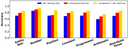
Lastly, we apply our structural decompositionbased abstractions on RAVEN sub-tasks which have multiple components, i.e., L-R , U-D , O-IC , and O-IG . The results are shown in Figure 8. First, just decomposing the task by its components improves the maximum accuracy on each task on average by about 20%. Additionally decomposing each component by its entity and layout attributes brings further gains, with GPT-3 175B reaching up to 77.6%, 78.0%, 82.8%, and 92.6% on L-R , U-D , O-IC , and O-IG respectively, and exceeding humans and nearing supervised baselines on the latter. The performance gain from this decomposition is again even more pronounced for smaller PLMs. Most significantly, OPT 1.3B improves from 20-30% accuracy to over 70% accuracy, nearing human performance. This demonstrates that not only is GPT-3 capable of very complex analogical reasoning tasks, but even PLMs less than 100 times its size can perform quite well here with the proper abstractions.
## 5.5 Fine-Grained Analysis
Finally, we analyze how model performance varies across different attributes and relations, as we introduce distracting attributes, and as we introduce rows into the matrix. In our analysis, we compare three representative levels of abstraction: entity attribute naming only (no decomposition into multiple prompts), decomposition of components , and full decomposition of entity and layout attributes and components .
## 5.5.1 Analysis of Attributes and Relations
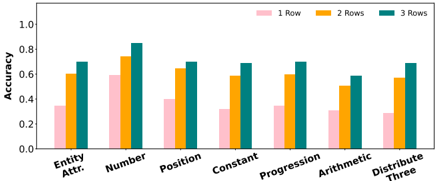
We measure the impact of abstractions in capturing each attribute and relation in RA VEN. In Figure 9,
Table 1: GPT-3 accuracy on Center sub-task with distracting orientation attribute in language prompts, under the naming and decomposition abstractions. orientation values are taken directly from RA VEN or randomly selected.
| Distractor Values | Naming | Decomposition |
|---------------------|----------|-----------------|
| RAVEN | 76.0% | 80.0% |
| Random | 72.6% | 77.8% |
we present GPT-3 175B's accuracy over each attribute and relation. We find that number is the best captured attribute even without any decomposition abstractions, while the model struggles with position until we introduce decomposition of attributes, suggesting the occupancy map encoding used here indeed helped capture it. Meanwhile, Arithmetic is the most difficult relation, with consistently lower accuracy than other relations.
## 5.5.2 Robustness to Distracting Attributes
Since our mappings from RAVEN attributes into language provide the key features over which relations occur, we may wonder how robust PLMs are to distracting or unimportant attributes. In fact, the RAVEN dataset includes one noise attribute that we excluded from our mapping to avoid unnecessarily increasing prompt lengths: orientation , i.e., the rotation of entities in the RPM. To begin exploring this issue, we incorporate orientation into the problem as a fourth entity-level attribute in addition to type , size , and color . For the best model (i.e., GPT-3) on the Center sub-task, we compare two possible injections of orientation values: using the values provided in RAVEN (which are mostly constant within each matrix row), and randomly selected values (which could be more distracting).
As shown in Table 1, compared to GPT-3's Center accuracies of 77.2% and 80.0% with respective naming and decomposition abstractions, the injection of orientation as a distraction feature does not degrade the model performance much, achieving accuracies of 76.0% and 80.0% when using values from RAVEN, and 72.6% and 77.8% when using random values. This shows that PLMs exhibit some robustness to distracting attributes in language context, and have the capability to ignore them in analogical reasoning. Future work may consider more in-depth analysis to discover the extent of model robustness to distraction features, and how it varies by model complexity.
Figure 8: PLM accuracy on multi-component RAVEN sub-tasks with attribute naming only, component decomposition, and full component and attribute decomposition, compared to supervised baselines and humans.
<details>
<summary>Image 8 Details</summary>
### Visual Description
## Chart: Accuracy vs. Model Size for Different Methods
### Overview
The image presents four separate line charts, arranged horizontally. Each chart depicts the accuracy of different methods (Human, Rel+AIR, CoPINet+ACL, Random, Attribute Naming, Compositional Decomposition, Compositional & Attribute Decomposition) as a function of model size, measured in billion parameters. The x-axis is logarithmic, ranging from 10^-1 to 10^2. The y-axis represents accuracy, ranging from 0 to 1. Each chart focuses on a different accuracy metric: L-R Accuracy, U-D Accuracy, O-IC Accuracy, and O-IG Accuracy.
### Components/Axes
* **X-axis:** Model Size (Billion Parameters) - Logarithmic scale with markers at 10^-1, 10^0 (1), 10^1, and 10^2.
* **Y-axis:** Accuracy - Linear scale from 0 to 1.
* **Legend:**
* Human (Green, dashed line)
* Rel+AIR (Blue, dotted line)
* CoPINet + ACL (Cyan, dash-dot line)
* Random (Black, dotted line)
* Attr. Naming (Blue, solid line)
* Comp. Decomp. (Red, solid line)
* Comp. & Attr. Decomp. (Yellow, solid line)
* **Chart Titles (Implicit):** L-R Accuracy, U-D Accuracy, O-IC Accuracy, and O-IG Accuracy. These are indicated by the y-axis labels.
### Detailed Analysis or Content Details
**Chart 1: L-R Accuracy**
* **Human:** Accuracy remains consistently high at approximately 0.95 throughout the model size range.
* **Rel+AIR:** Accuracy starts at approximately 0.1 and remains relatively flat around 0.15.
* **CoPINet + ACL:** Accuracy starts at approximately 0.1 and increases to around 0.25 at 10^2.
* **Random:** Accuracy starts at approximately 0.05 and increases to around 0.15 at 10^2.
* **Attr. Naming:** Accuracy starts at approximately 0.05 and increases sharply to around 0.7 at 10^2.
* **Comp. Decomp.:** Accuracy starts at approximately 0.1 and increases to around 0.6 at 10^2.
* **Comp. & Attr. Decomp.:** Accuracy starts at approximately 0.2 and increases to around 0.75 at 10^2.
**Chart 2: U-D Accuracy**
* **Human:** Accuracy remains consistently high at approximately 1.0 throughout the model size range.
* **Rel+AIR:** Accuracy remains relatively flat around 0.8 throughout the model size range.
* **CoPINet + ACL:** Accuracy starts at approximately 0.6 and increases to around 0.85 at 10^2.
* **Random:** Accuracy starts at approximately 0.05 and increases to around 0.2 at 10^2.
* **Attr. Naming:** Accuracy starts at approximately 0.1 and increases to around 0.7 at 10^2.
* **Comp. Decomp.:** Accuracy starts at approximately 0.3 and increases to around 0.75 at 10^2.
* **Comp. & Attr. Decomp.:** Accuracy starts at approximately 0.4 and increases to around 0.85 at 10^2.
**Chart 3: O-IC Accuracy**
* **Human:** Accuracy remains consistently high at approximately 1.0 throughout the model size range.
* **Rel+AIR:** Accuracy remains relatively flat around 0.8 throughout the model size range.
* **CoPINet + ACL:** Accuracy starts at approximately 0.2 and increases to around 0.7 at 10^2.
* **Random:** Accuracy starts at approximately 0.05 and increases to around 0.2 at 10^2.
* **Attr. Naming:** Accuracy starts at approximately 0.1 and increases to around 0.75 at 10^2.
* **Comp. Decomp.:** Accuracy starts at approximately 0.2 and increases to around 0.7 at 10^2.
* **Comp. & Attr. Decomp.:** Accuracy starts at approximately 0.3 and increases to around 0.85 at 10^2.
**Chart 4: O-IG Accuracy**
* **Human:** Accuracy remains consistently high at approximately 1.0 throughout the model size range.
* **Rel+AIR:** Accuracy remains relatively flat around 0.8 throughout the model size range.
* **CoPINet + ACL:** Accuracy starts at approximately 0.1 and increases to around 0.6 at 10^2.
* **Random:** Accuracy starts at approximately 0.05 and increases to around 0.2 at 10^2.
* **Attr. Naming:** Accuracy starts at approximately 0.1 and increases to around 0.7 at 10^2.
* **Comp. Decomp.:** Accuracy starts at approximately 0.2 and increases to around 0.7 at 10^2.
* **Comp. & Attr. Decomp.:** Accuracy starts at approximately 0.3 and increases to around 0.8 at 10^2.
### Key Observations
* Human performance consistently achieves the highest accuracy across all metrics.
* The "Random" method consistently exhibits the lowest accuracy.
* All methods, except "Human" and "Rel+AIR", show a clear positive correlation between model size and accuracy – accuracy increases as the model size grows.
* "Comp. & Attr. Decomp." generally outperforms "Comp. Decomp." and "Attr. Naming" across all metrics.
* "Rel+AIR" shows minimal improvement in accuracy with increasing model size.
### Interpretation
The charts demonstrate the impact of model size on the performance of different methods for a set of accuracy metrics (L-R, U-D, O-IC, O-IG). The consistent high performance of the "Human" baseline suggests a ceiling for achievable accuracy. The significant improvement in accuracy with increasing model size for methods like "Attr. Naming", "Comp. Decomp.", and "Comp. & Attr. Decomp." indicates that these methods benefit from larger model capacities. The relatively flat performance of "Rel+AIR" suggests that its performance is less sensitive to model size, potentially indicating a limitation in its approach or a saturation point. The "Comp. & Attr. Decomp." method consistently achieves the highest accuracy among the automated methods, suggesting that combining compositional and attribute decomposition is a promising approach. The low performance of the "Random" method serves as a baseline for evaluating the effectiveness of the other methods. The different accuracy metrics (L-R, U-D, O-IC, O-IG) likely represent different aspects of the task, and the varying performance of the methods across these metrics suggests that different methods excel at different aspects of the task.
</details>
Figure 9: Comparison of accuracy on examples from all sub-tasks, broken down by the types of attributes and relations they require capturing.
<details>
<summary>Image 9 Details</summary>
### Visual Description
\n
## Bar Chart: Accuracy Comparison of Decomposition Methods
### Overview
This image presents a bar chart comparing the accuracy of three different decomposition methods ("Attr. Naming Only", "Component Decomp.", and "Component + Attr. Decomp.") across seven different categories: "Entity Attr.", "Number", "Position", "Constant", "Progression", "Arithmetic", and "Distribute Three". The y-axis represents accuracy, ranging from 0.0 to 1.0.
### Components/Axes
* **X-axis:** Categories - "Entity Attr.", "Number", "Position", "Constant", "Progression", "Arithmetic", "Distribute Three".
* **Y-axis:** Accuracy, labeled from 0.0 to 1.0 with increments of 0.2.
* **Legend:** Located at the top-center of the chart.
* Blue: "Attr. Naming Only"
* Red: "Component Decomp."
* Yellow: "Component + Attr. Decomp."
### Detailed Analysis
The chart consists of seven groups of three bars, one for each decomposition method within each category.
* **Entity Attr.:**
* Attr. Naming Only (Blue): Approximately 0.74
* Component Decomp. (Red): Approximately 0.82
* Component + Attr. Decomp. (Yellow): Approximately 0.88
* **Number:**
* Attr. Naming Only (Blue): Approximately 0.86
* Component Decomp. (Red): Approximately 0.91
* Component + Attr. Decomp. (Yellow): Approximately 0.95
* **Position:**
* Attr. Naming Only (Blue): Approximately 0.68
* Component Decomp. (Red): Approximately 0.72
* Component + Attr. Decomp. (Yellow): Approximately 0.92
* **Constant:**
* Attr. Naming Only (Blue): Approximately 0.72
* Component Decomp. (Red): Approximately 0.78
* Component + Attr. Decomp. (Yellow): Approximately 0.84
* **Progression:**
* Attr. Naming Only (Blue): Approximately 0.69
* Component Decomp. (Red): Approximately 0.79
* Component + Attr. Decomp. (Yellow): Approximately 0.86
* **Arithmetic:**
* Attr. Naming Only (Blue): Approximately 0.62
* Component Decomp. (Red): Approximately 0.68
* Component + Attr. Decomp. (Yellow): Approximately 0.75
* **Distribute Three:**
* Attr. Naming Only (Blue): Approximately 0.72
* Component Decomp. (Red): Approximately 0.78
* Component + Attr. Decomp. (Yellow): Approximately 0.86
**Trends:**
* "Component + Attr. Decomp." (Yellow) consistently achieves the highest accuracy across all categories.
* "Component Decomp." (Red) generally outperforms "Attr. Naming Only" (Blue).
* The accuracy varies significantly across categories, with "Number" showing the highest overall accuracy and "Arithmetic" the lowest.
### Key Observations
* The "Component + Attr. Decomp." method demonstrates a clear advantage in accuracy compared to the other two methods.
* The "Arithmetic" category consistently yields the lowest accuracy scores for all methods.
* The "Position" category shows the largest improvement when using "Component + Attr. Decomp." compared to "Attr. Naming Only".
### Interpretation
The data suggests that combining component decomposition with attribute naming provides the most accurate results across a range of categories. This indicates that leveraging both the structural and semantic information of the data leads to improved performance. The consistently lower accuracy in the "Arithmetic" category might suggest that this type of data presents unique challenges for these decomposition methods, potentially requiring specialized techniques. The large gains observed in "Position" when using the combined method suggest that attribute naming is particularly helpful in disambiguating positional information. Overall, the chart highlights the benefits of a holistic approach to data decomposition, integrating both component-based and attribute-based analysis.
</details>
## 5.5.3 In-Context Learning Over Rows
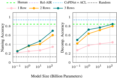
By design, RPM tasks are meant to require minimal background knowledge. They should be impossible to solve without the first two rows of the matrix, which provide essential context to complete the third row of the matrix. To understand whether PLMs capture relations specifically from in-context learning over the first two rows of the matrix (as opposed to using prior knowledge from pre-training), we measure the model performance as we introduce rows to the matrices.
As shown in Figure 10, the average model performance increases across all sizes and abstractions as rows are added to the matrix. This suggests that in-context learning indeed contributes significantly to performance, even for smaller models. Larger model sizes see the most significant improvements, suggesting that larger PLMs are stronger in-context learners than smaller ones. Further, larger PLMs can achieve nearly the same accuracy with only two rows of the matrix provided rather compared to having all three, suggesting that they pick up the task quite quickly from in-context learning.
We also observe that in many cases, models achieve accuracies above chance (12.5% accuracy) without being provided any complete rows of the
Table 2: GPT-3 accuracy on RAVEN sub-tasks as rows are added to the RPM, under only naming abstractions.
| Sub-Task | 1 Row | 2 Rows | 3 Rows | Human |
|------------|---------|----------|----------|---------|
| Center | 36.8% | 69.2% | 77.2% | 95.6% |
| 2x2Grid | 54.0% | 71.0% | 78.0% | 81.8% |
| 3x3Grid | 73.0% | 85.2% | 86.4% | 79.6% |
| L-R | 14.0% | 38.2% | 54.2% | 86.4% |
| U-D | 12.4% | 42.0% | 53.6% | 81.8% |
| O-IC | 19.6% | 53.6% | 64.8% | 86.4% |
| O-IG | 32.0% | 62.2% | 74.8% | 81.8% |
matrix (only the third, incomplete row). This may suggest the PLM has a useful prior for this problem, despite it being a visual problem and thus impossible to observe directly in pre-training. This raises questions about the objectivity of RA VEN and possibly the RPM task. 11 Further, when decomposition abstractions are applied, models achieve higher accuracies than when not, suggesting that decomposition encodes some of this prior knowledge for the task. In Table 2, we take a closer look at GPT-3 175B's performance within sub-tasks. Surprisingly, we find the highest accuracies on the grid-based sub-tasks, despite them being the most difficult tasks for humans.
This motivates future work to compare human and PLM performance on ablated analogy-making tasks like these to further evaluate their objectiveness and identify commonalities. Future work in AI and analogy may also consider building diagnostic datasets to tease apart attribute and relation types to better understand how they contribute to model performance and identify areas for improvement.
## In-context learning of attributes and relations.
11 In Appendix B, we further explore this hypothesis on the Impartial-RAVEN dataset (Hu et al., 2021) that removes some superficial correlations in matrix completion choices, and still see comparable results.
Figure 10: Macro average accuracy over all RAVEN sub-tasks as we introduce rows to the matrix during incontext learning, under naming abstractions only (left) and all naming and decomposition abstractions (right). In 1 Row, we include only the incomplete third row.
<details>
<summary>Image 10 Details</summary>
### Visual Description
## Charts: Naming Accuracy vs. Decomposition Accuracy by Model Size and Rows
### Overview
The image presents two line charts comparing the performance of different models (Human, Rel-AIR, CoPINet + ACL, and Random) on two tasks: Naming Accuracy and Decomposition Accuracy. Both charts share the same x-axis representing Model Size (in Billion Parameters) and vary by the number of Rows used (1, 2, or 3). The charts visually demonstrate how performance changes with increasing model size for each model and row configuration.
### Components/Axes
* **X-axis:** Model Size (Billion Parameters) - Scale is logarithmic: 10<sup>-1</sup>, 10<sup>0</sup>, 10<sup>1</sup>, 10<sup>2</sup>.
* **Left Chart Y-axis:** Naming Accuracy - Scale is linear from 0 to 1.
* **Right Chart Y-axis:** Decomposition Accuracy - Scale is linear from 0 to 1.
* **Legend:**
* Human (Green, dashed line)
* Rel-AIR (Purple line)
* CoPINet + ACL (Blue line)
* Random (Black, dotted line)
* **Data Series:**
* 1 Row (Pink, light shade)
* 2 Rows (Orange)
* 3 Rows (Dark Blue)
### Detailed Analysis or Content Details
**Left Chart: Naming Accuracy**
* **Human (Green, dashed):** Maintains a consistently high Naming Accuracy of approximately 0.95 across all model sizes.
* **Random (Black, dotted):** Maintains a consistently low Naming Accuracy of approximately 0.2 across all model sizes.
* **Rel-AIR (Purple):**
* At 10<sup>-1</sup> Billion Parameters: Approximately 0.22
* At 10<sup>0</sup> Billion Parameters: Approximately 0.35
* At 10<sup>1</sup> Billion Parameters: Approximately 0.52
* At 10<sup>2</sup> Billion Parameters: Approximately 0.65
* **CoPINet + ACL (Blue):**
* 1 Row (Pink):
* At 10<sup>-1</sup> Billion Parameters: Approximately 0.23
* At 10<sup>0</sup> Billion Parameters: Approximately 0.33
* At 10<sup>1</sup> Billion Parameters: Approximately 0.46
* At 10<sup>2</sup> Billion Parameters: Approximately 0.60
* 2 Rows (Orange):
* At 10<sup>-1</sup> Billion Parameters: Approximately 0.28
* At 10<sup>0</sup> Billion Parameters: Approximately 0.40
* At 10<sup>1</sup> Billion Parameters: Approximately 0.55
* At 10<sup>2</sup> Billion Parameters: Approximately 0.70
* 3 Rows (Dark Blue):
* At 10<sup>-1</sup> Billion Parameters: Approximately 0.32
* At 10<sup>0</sup> Billion Parameters: Approximately 0.45
* At 10<sup>1</sup> Billion Parameters: Approximately 0.60
* At 10<sup>2</sup> Billion Parameters: Approximately 0.75
**Right Chart: Decomposition Accuracy**
* **Human (Green, dashed):** Maintains a consistently high Decomposition Accuracy of approximately 0.9 across all model sizes.
* **Random (Black, dotted):** Maintains a consistently low Decomposition Accuracy of approximately 0.2 across all model sizes.
* **Rel-AIR (Purple):**
* At 10<sup>-1</sup> Billion Parameters: Approximately 0.55
* At 10<sup>0</sup> Billion Parameters: Approximately 0.65
* At 10<sup>1</sup> Billion Parameters: Approximately 0.75
* At 10<sup>2</sup> Billion Parameters: Approximately 0.85
* **CoPINet + ACL (Blue):**
* 1 Row (Pink):
* At 10<sup>-1</sup> Billion Parameters: Approximately 0.25
* At 10<sup>0</sup> Billion Parameters: Approximately 0.40
* At 10<sup>1</sup> Billion Parameters: Approximately 0.55
* At 10<sup>2</sup> Billion Parameters: Approximately 0.65
* 2 Rows (Orange):
* At 10<sup>-1</sup> Billion Parameters: Approximately 0.45
* At 10<sup>0</sup> Billion Parameters: Approximately 0.60
* At 10<sup>1</sup> Billion Parameters: Approximately 0.75
* At 10<sup>2</sup> Billion Parameters: Approximately 0.85
* 3 Rows (Dark Blue):
* At 10<sup>-1</sup> Billion Parameters: Approximately 0.50
* At 10<sup>0</sup> Billion Parameters: Approximately 0.65
* At 10<sup>1</sup> Billion Parameters: Approximately 0.80
* At 10<sup>2</sup> Billion Parameters: Approximately 0.90
### Key Observations
* **Model Size Impact:** For all models except Human and Random, performance (both Naming and Decomposition Accuracy) generally increases with increasing model size.
* **Rows Impact:** Increasing the number of rows consistently improves performance for CoPINet + ACL, with 3 rows generally outperforming 2 and 1 rows.
* **Human Performance:** Human performance is significantly higher than all other models on both tasks, indicating a performance ceiling.
* **Random Performance:** Random performance is consistently low, serving as a baseline.
* **Rel-AIR:** Rel-AIR shows a steady increase in performance with model size, but remains below Human performance.
### Interpretation
The data suggests that increasing model size generally leads to improved performance in both Naming and Decomposition tasks, particularly for the CoPINet + ACL model. The benefit of increasing the number of rows used in CoPINet + ACL indicates that the model benefits from more complex representations or contextual information. The consistently high performance of the Human baseline highlights the gap between current model capabilities and human-level performance. The low performance of the Random model confirms that the observed performance of other models is not due to chance. The charts demonstrate a clear trade-off between model complexity (size and row count) and performance, with diminishing returns as models approach human-level accuracy. The difference in performance between the two tasks (Naming vs. Decomposition) suggests that the models may have varying strengths and weaknesses in different aspects of language understanding.
</details>
Figure 11: Comparison of accuracy on examples from all RAVEN sub-tasks as rows are introduced to the matrix, with only entity attribute naming abstractions .
<details>
<summary>Image 11 Details</summary>
### Visual Description
\n
## Bar Chart: Accuracy vs. Problem Type & Row Count
### Overview
This image presents a bar chart comparing the accuracy of a system or method across different problem types, categorized by the number of rows involved. The x-axis represents the problem type, and the y-axis represents the accuracy score. Three different row counts (1, 2, and 3) are represented by different colored bars for each problem type.
### Components/Axes
* **X-axis:** Problem Type - with categories: "Entity Attr.", "Number", "Position", "Constant", "Progression", "Arithmetic", "Distribute Three".
* **Y-axis:** Accuracy - Scale ranges from 0.0 to 1.0, with increments of 0.2.
* **Legend:** Located at the top-right corner.
* Pink: 1 Row
* Orange: 2 Rows
* Teal: 3 Rows
### Detailed Analysis
The chart consists of seven groups of three bars, one for each problem type and row count combination.
* **Entity Attr.:**
* 1 Row (Pink): Approximately 0.35
* 2 Rows (Orange): Approximately 0.65
* 3 Rows (Teal): Approximately 0.60
* **Number:**
* 1 Row (Pink): Approximately 0.55
* 2 Rows (Orange): Approximately 0.75
* 3 Rows (Teal): Approximately 0.85
* **Position:**
* 1 Row (Pink): Approximately 0.40
* 2 Rows (Orange): Approximately 0.65
* 3 Rows (Teal): Approximately 0.65
* **Constant:**
* 1 Row (Pink): Approximately 0.30
* 2 Rows (Orange): Approximately 0.60
* 3 Rows (Teal): Approximately 0.60
* **Progression:**
* 1 Row (Pink): Approximately 0.55
* 2 Rows (Orange): Approximately 0.60
* 3 Rows (Teal): Approximately 0.70
* **Arithmetic:**
* 1 Row (Pink): Approximately 0.50
* 2 Rows (Orange): Approximately 0.55
* 3 Rows (Teal): Approximately 0.70
* **Distribute Three:**
* 1 Row (Pink): Approximately 0.30
* 2 Rows (Orange): Approximately 0.60
* 3 Rows (Teal): Approximately 0.65
### Key Observations
* Generally, accuracy increases with the number of rows for most problem types.
* The "Number" problem type consistently shows the highest accuracy, especially with 3 rows.
* "Entity Attr.", "Constant", and "Distribute Three" have the lowest accuracy scores, particularly with only 1 row.
* The difference in accuracy between 2 and 3 rows is less pronounced than the difference between 1 and 2 rows.
### Interpretation
The data suggests that the system's performance improves with increased complexity (more rows) for most problem types. This could indicate that the system benefits from having more data points to work with, or that the additional rows help to disambiguate the problem. The consistently high accuracy on "Number" problems suggests that the system is particularly well-suited for tasks involving numerical reasoning. The lower accuracy on "Entity Attr.", "Constant", and "Distribute Three" problems may indicate that these problem types are inherently more difficult, or that the system requires further training on these types of problems. The diminishing returns in accuracy gains between 2 and 3 rows could suggest a point of saturation, where adding more rows does not significantly improve performance.
</details>
We may wonder whether specific relations or attributes are easier to understand than others with less context. For example, the Progression or Constant relations may be possible to recognize only from the first two items of the third row in an RPM, as we can easily observe patterns in attribute values here, e.g., that entity size is increasing or color remains constant. In Figures 11 and 12, we surprisingly observe only marginal differences here, except for the number attribute, which seems significantly better captured than other attributes in this no-context setting.
Figure 12: Comparison of accuracy on examples from all RAVEN sub-tasks as rows are introduced to the matrix, with all decomposition abstractions .
<details>
<summary>Image 12 Details</summary>
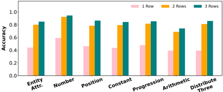
### Visual Description
## Bar Chart: Accuracy vs. Problem Type with Varying Row Counts
### Overview
This image presents a bar chart comparing the accuracy of a system or model across different problem types, evaluated with varying numbers of rows in the input data. The x-axis represents the problem type, and the y-axis represents the accuracy. Three different row counts (1, 2, and 3) are represented by different colored bars for each problem type.
### Components/Axes
* **X-axis:** Problem Type. Categories are: "Entity Attr.", "Number", "Position", "Constant", "Progression", "Arithmetic", "Distribute Three".
* **Y-axis:** Accuracy, ranging from 0.0 to 1.0, with increments of 0.2.
* **Legend:** Located in the top-right corner.
* Pink: 1 Row
* Orange: 2 Rows
* Teal: 3 Rows
### Detailed Analysis
The chart consists of seven groups of three bars, one for each problem type. I will analyze each problem type individually, noting the approximate accuracy for each row count.
* **Entity Attr.:**
* 1 Row (Pink): Approximately 0.45
* 2 Rows (Orange): Approximately 0.82
* 3 Rows (Teal): Approximately 0.85
* **Number:**
* 1 Row (Pink): Approximately 0.62
* 2 Rows (Orange): Approximately 0.94
* 3 Rows (Teal): Approximately 0.96
* **Position:**
* 1 Row (Pink): Approximately 0.43
* 2 Rows (Orange): Approximately 0.79
* 3 Rows (Teal): Approximately 0.83
* **Constant:**
* 1 Row (Pink): Approximately 0.73
* 2 Rows (Orange): Approximately 0.81
* 3 Rows (Teal): Approximately 0.85
* **Progression:**
* 1 Row (Pink): Approximately 0.76
* 2 Rows (Orange): Approximately 0.82
* 3 Rows (Teal): Approximately 0.85
* **Arithmetic:**
* 1 Row (Pink): Approximately 0.68
* 2 Rows (Orange): Approximately 0.74
* 3 Rows (Teal): Approximately 0.79
* **Distribute Three:**
* 1 Row (Pink): Approximately 0.35
* 2 Rows (Orange): Approximately 0.79
* 3 Rows (Teal): Approximately 0.92
**Trends:**
Generally, accuracy increases with the number of rows for most problem types. The pink bars (1 Row) are consistently the lowest, while the teal bars (3 Rows) are often the highest.
### Key Observations
* The "Distribute Three" problem type shows the most significant improvement in accuracy as the number of rows increases, starting at a low accuracy of approximately 0.35 with 1 row and reaching approximately 0.92 with 3 rows.
* The "Constant" problem type has relatively high accuracy even with only 1 row (approximately 0.73), suggesting it is easier to solve.
* The "Arithmetic" problem type shows the smallest improvement in accuracy with increasing rows.
* The "Number" problem type consistently achieves high accuracy across all row counts, with values above 0.9 for 2 and 3 rows.
### Interpretation
The data suggests that increasing the amount of input data (represented by the number of rows) generally improves the accuracy of the system/model across most problem types. This is expected, as more data typically allows for better learning and generalization. The large improvement observed for "Distribute Three" indicates that this problem type is particularly data-dependent. The relatively stable accuracy of "Constant" suggests that this problem type is inherently simpler or requires less data to solve effectively. The differences in accuracy between the row counts highlight the importance of data quantity for certain problem types, and the potential for diminishing returns as the number of rows increases (as seen in "Arithmetic"). The chart provides a comparative analysis of the model's performance on different problem types and the impact of data volume on its accuracy.
</details>
## 6 Conclusion
In this work, we explored the ability of large PLMs to perform zero-shot analogical reasoning in visual Raven's Progressive Matrices (RPM). Upon the simplest mapping to language, they can achieve striking results, while applying higher-level naming and decomposition abstractions over the task features further raises performance to the level of humans and supervised approaches in some cases. We find that while ordinal naming abstractions are a powerful way to enable analogical reasoning in larger PLMs, decomposition abstractions that break the task down into atomic parts conserve their working memory such that even smaller PLMs under 1B parameters can achieve competitive performance on this challenging problem.
Our detailed analysis revealed insights about which features of the task PLMs best capture, their robustness to distracting features, and the role of in-context learning and prior knowledge in picking up this complex task. Surprisingly, we find that even without two complete rows of prior context from the matrix, GPT-3 175B and smaller models can achieve above-chance performance on the task, raising questions about the objectivity and true role of prior knowledge in RPM tasks, which are assumed to require minimal prior knowledge.
These results also raise some questions about the role PLMs may play in future AI systems capable of analogy. While previously thought to be a difficult problem for AI systems, PLMs can solve the reasoning step of analogy easily given strong abstractions over visual perception. Many of these abstractions are intuitive and commonly researched in computer vision, including the detection of object types, sizes, colors, counts, and global arrangements. As such, future work may dive deeper into the challenging problem of generalized perception across domains, where we must robustly tease apart the key features of tasks and experiences that may facilitate analogy-making, e.g., in recognizing the commonalities between a physical bridge and the bridge of a song (Mitchell, 2021). Recent efforts toward understanding how humans describe abstract visual features in language by mapping them to natural concepts 12 are a promising direction toward this goal (Lachmy et al., 2022; Ji et al., 2022).
12 For example, when communicating about abstract shapes, we may make an analogy to refer to them as looking like more familiar natural concepts like flowers or dog bones.
## Acknowledgements
This work was supported in part by DARPA PTG program HR00112220003. We would like to thank the anonymous reviewers for their valuable comments and suggestions.
## Limitations
## Perception and reasoning in text-based RAVEN.
In this work, one limitation is that we do not attempt to solve the perception problem of analogymaking in RPM, rather we apply perfect perception in solving the reasoning part, and assume the perception problem is simple. By doing so, we find that PLMs may be a strong solution to the reasoning problem here, which may better direct future efforts toward AI and analogy. Obviously, the perception problem for idealized domains is a lot different than more natural domains, and identifying key features across many domains that can facilitate a mapping is still a challenging unsolved problem. We hope that our work sparks more interest in this problem.
Meanwhile, one may argue that our decomposition abstractions are too strong, and actually contribute to the reasoning problem in RPM, as they make an independence assumption about which features of the task can be teased apart. Making such an assumption requires an understanding of the problem that cannot be inferred by only seeing one instance. However, we decomposed the task based on very intuitive and common attributes, e.g., shapes, colors, sizes, and counts of items. We believe that the strength of such an abstraction, which could be applied in many problems, should not be understated. Nonetheless, we include decomposition-free forms of results as much as possible throughout the paper to help compare the contributions of decomposition versus naming abstractions, which is more clearly only providing perceptual information. In fact, we find that without any decomposition, PLMs still achieve very strong performance in many cases, and performance gains from decomposition are not always large.
Human performance. Lastly, we note some limitations in the human performance measurements used as reference points. In Zhang et al. (2019a), human performance on RAVEN was measured by giving subjects some task-specific training, then evaluating them on the original visual form of the task. This differs from our results in two ways. First, PLMs had no task-specific training for RAVEN, given that experiments were zero-shot and the text data we generate is new and thus impossible to appear directly in PLM pre-training. This may give humans an advantage. Second, the task is presented to PLMs in text form, not visually. While the essential information from the task is preserved by our conversion, it is possible that this conversion would affect the difficulty of the task for humans (making it easier or harder). As such, it becomes unclear how to contextualize our results with these past human results. Future work may carry out systematic human studies to compare the analogical reasoning capabilities of humans and PLMs in different settings.
## Ethical Considerations
This work does not use any human subjects or human-generated data. Our work deals with abstract visual features that are described with numerical symbols, thus not strongly targeting any language. A possible ethical concern for this work is the amount of computational resources used in evaluating PLMs. To reduce unnecessary computation in our study, we chose to apply PLMs to only a subset of 500 testing examples from each sub-task of the RAVEN dataset, while the full testing set is four times as large.
## References
Yonatan Bitton, Ron Yosef, Eli Strugo, Dafna Shahaf, Roy Schwartz, and Gabriel Stanovsky. 2022. VASR: Visual analogies of situation recognition. In Proceedings of the AAAI Conference on Artificial Intelligence (AAAI) .
Tom Brown, Benjamin Mann, Nick Ryder, Melanie Subbiah, Jared D Kaplan, Prafulla Dhariwal, Arvind Neelakantan, Pranav Shyam, Girish Sastry, Amanda Askell, et al. 2020. Language models are few-shot learners. Advances in neural information processing systems , 33:1877-1901.
Jiangjie Chen, Rui Xu, Ziquan Fu, Wei Shi, Zhongqiao Li, Xinbo Zhang, Changzhi Sun, Lei Li, Yanghua Xiao, and Hao Zhou. 2022. E-KAR: A benchmark for rationalizing natural language analogical reasoning. In Findings of the Association for Computational Linguistics: ACL 2022 , pages 3941-3955, Dublin, Ireland. Association for Computational Linguistics.
Stella Christie and Dedre Gentner. 2014. Language helps children succeed on a classic analogy task. Cognitive Science , 38(2):383-397.
- Dedre Gentner. 1983. Structure-mapping: A theoretical framework for analogy. Cognitive Science , 7(2):155170.
- Dedre Gentner. 2010. Bootstrapping the mind: Analogical processes and symbol systems. Cognitive Science , 34(5):752-775.
- Dedre Gentner, Asli Özyürek, Özge Gürcanli, and Susan Goldin-Meadow. 2013. Spatial language facilitates spatial cognition: Evidence from children who lack language input. Cognition , 127(3):318-330.
- Peter Gordon. 2004. Numerical cognition without words: Evidence from Amazonia. Science , 306(5695):496-499.
- Felix Hill, Adam Santoro, David GT Barrett, Ari S Morcos, and Timothy Lillicrap. 2019. Learning to make analogies by contrasting abstract relational structure. In 7th International Conference on Learning Representations (ICLR) .
- Douglas R Hofstadter and Melanie Mitchell. 1994. The Copycat project: A model of mental fluidity and analogy-making , pages 31-112. Ablex Publishing.
- Douglas R Hofstadter and Emmanuel Sander. 2013. Surfaces and essences: Analogy as the fuel and fire of thinking . Basic Books.
- Keith J Holyoak. 1984. Analogical thinking and human intelligence. Advances in the psychology of human intelligence , 2:199-230.
- Keith J Holyoak. 2012. Analogy and relational reasoning. The Oxford Handbook of Thinking and Reasoning .
- Sheng Hu, Yuqing Ma, Xianglong Liu, Yanlu Wei, and Shihao Bai. 2021. Stratified rule-aware network for abstract visual reasoning. In Proceedings of the AAAI Conference on Artificial Intelligence (AAAI) , volume 35, pages 1567-1574.
- Anya Ji, Noriyuki Kojima, Noah Rush, Alane Suhr, Wai Keen Vong, Robert Hawkins, and Yoav Artzi. 2022. Abstract visual reasoning with tangram shapes. In Proceedings of the 2022 Conference on Empirical Methods in Natural Language Processing , Abu Dhabi, United Arab Emirates. Association for Computational Linguistics.
- Youngsung Kim, Jinwoo Shin, Eunho Yang, and Sung Ju Hwang. 2020. Few-shot visual reasoning with meta-analogical contrastive learning. In Advances in Neural Information Processing Systems , volume 33, pages 16846-16856. Curran Associates, Inc.
- Royi Lachmy, Valentina Pyatkin, Avshalom Manevich, and Reut Tsarfaty. 2022. Draw Me a Flower: Processing and Grounding Abstraction in Natural Language. Transactions of the Association for Computational Linguistics , 10:1341-1356.
- Brenden M Lake, Ruslan Salakhutdinov, and Joshua B Tenenbaum. 2015. Human-level concept learning through probabilistic program induction. Science , 350(6266):1332-1338.
- Frank J Lee and John R Anderson. 2001. Does learning a complex task have to be complex?: A study in learning decomposition. Cognitive Psychology , 42(3):267-316.
- Peng-Hsuan Li, Tsan-Yu Yang, and Wei-Yun Ma. 2020. CA-EHN: Commonsense analogy from E-HowNet. In Proceedings of the Twelfth Language Resources and Evaluation Conference , pages 2984-2990, Marseille, France. European Language Resources Association.
- Tal Linzen. 2016. Issues in evaluating semantic spaces using word analogies. In Proceedings of the 1st Workshop on Evaluating Vector-Space Representations for NLP , pages 13-18, Berlin, Germany. Association for Computational Linguistics.
- Hongjing Lu, Ying Nian Wu, and Keith J Holyoak. 2019. Emergence of analogy from relation learning. Proceedings of the National Academy of Sciences , 116(10):4176-4181.
- Mikołaj Małki´ nski and Jacek Ma´ ndziuk. 2022. Deep learning methods for abstract visual reasoning: A survey on Raven's Progressive Matrices. arXiv preprint arXiv:2201.12382 .
- Tomas Mikolov, Ilya Sutskever, Kai Chen, Greg S Corrado, and Jeff Dean. 2013a. Distributed representations of words and phrases and their compositionality. Advances in Neural Information Processing Systems , 26.
- Tomas Mikolov, Wen-tau Yih, and Geoffrey Zweig. 2013b. Linguistic regularities in continuous space word representations. In Proceedings of the 2013 Conference of the North American Chapter of the Association for Computational Linguistics: Human Language Technologies , pages 746-751, Atlanta, Georgia. Association for Computational Linguistics.
- Melanie Mitchell. 2021. Abstraction and analogymaking in artificial intelligence. Annals of the New York Academy of Sciences , 1505(1):79-101.
- Victor Vikram Odouard and Melanie Mitchell. 2022. Evaluating understanding on conceptual abstraction benchmarks. In Proceedings of the AI Evaluation Beyond Metrics at IJCAI-ECAI 2022 , Vienna, Austria.
- Long Ouyang, Jeff Wu, Xu Jiang, Diogo Almeida, Carroll L Wainwright, Pamela Mishkin, Chong Zhang, Sandhini Agarwal, Katarina Slama, Alex Ray, et al. 2022. Training language models to follow instructions with human feedback. arXiv preprint arXiv:2203.02155 .
- Roma Patel and Ellie Pavlick. 2021. Mapping language models to grounded conceptual spaces. In International Conference on Learning Representations .
- John C Raven and JH Court. 1938. Raven's progressive matrices . Western Psychological Services Los Angeles.
- Lynn C Robertson and Marvin R Lamb. 1991. Neuropsychological contributions to theories of part/whole organization. Cognitive Psychology , 23(2):299-330.
- Robyn Speer, Catherine Havasi, and Henry Lieberman. 2008. Analogyspace: Reducing the dimensionality of common sense knowledge. In AAAI , volume 8, pages 548-553.
- Steven Spratley, Krista Ehinger, and Tim Miller. 2020. Acloser look at generalisation in raven. In Computer Vision - ECCV 2020: 16th European Conference, Glasgow, UK, August 23-28, 2020, Proceedings, Part XXVII , page 601-616, Berlin, Heidelberg. SpringerVerlag.
- Oren Sultan and Dafna Shahaf. 2022. Life is a circus and we are the clowns: Automatically finding analogies between situations and processes. In Proceedings of the 2022 Conference on Empirical Methods in Natural Language Processing , Abu Dhabi, United Arab Emirates. Association for Computational Linguistics.
- Damien Teney, Peng Wang, Jiewei Cao, Lingqiao Liu, Chunhua Shen, and Anton van den Hengel. 2020. Vprom: A benchmark for visual reasoning using visual progressive matrices. In Proceedings of the AAAI Conference on Artificial Intelligence , volume 34, pages 12071-12078.
- Peter D Turney. 2008. The latent relation mapping engine: Algorithm and experiments. Journal of Artificial Intelligence Research , 33:615-655.
- Peter D Turney, Michael L Littman, Jeffrey Bigham, and Victor Shnayder. 2003. Combining independent modules in lexical multiple-choice problems. Recent Advances in Natural Language Processing III: Selected Papers from RANLP , 2003:101-110.
- Taylor Webb, Keith J Holyoak, and Hongjing Lu. 2022. Emergent analogical reasoning in large language models. arXiv preprint arXiv:2212.09196 .
- Chi Zhang, Feng Gao, Baoxiong Jia, Yixin Zhu, and Song-Chun Zhu. 2019a. RAVEN: A dataset for relational and analogical visual reasoning. In Proceedings of the IEEE Conference on Computer Vision and Pattern Recognition (CVPR) .
- Chi Zhang, Baoxiong Jia, Feng Gao, Yixin Zhu, HongJing Lu, and Song-Chun Zhu. 2019b. Learning perceptual inference by contrasting. In Advances in Neural Information Processing Systems , volume 32. Curran Associates, Inc.
- Chi Zhang, Baoxiong Jia, Song-Chun Zhu, and Yixin Zhu. 2021. Abstract spatial-temporal reasoning via
probabilistic abduction and execution. In Proceedings of the IEEE/CVF Conference on Computer Vision and Pattern Recognition (CVPR) , pages 97369746.
- Susan Zhang, Stephen Roller, Naman Goyal, Mikel Artetxe, Moya Chen, Shuohui Chen, Christopher Dewan, Mona Diab, Xian Li, Xi Victoria Lin, et al. 2022. OPT: Open pre-trained transformer language models. arXiv preprint arXiv:2205.01068 .
## A Expanded Results
In Table 3, we present additional results with a wider range of OPT model sizes (Zhang et al., 2022). We observe similar mostly monotonic increases of accuracy with model size.
## B Results and Analysis with I-RAVEN
As the generation strategy for the negative choices in RAVEN can introduce distributional bias that is problematic for supervised learning and leads to artificially high performance (Hu et al., 2021), this could be a possible reason behind PLMs' strong performance on the task even without any complete rows of context. As such, in Table 4 and Figure 13, we include some supplementary analysis on the Impartial-RAVEN (I-RAVEN) dataset from Hu et al., which introduces more variation in negative choices. However, we observe similar performance trends in I-RAVEN. Performance mostly monotonically increases with model sizes and more abstraction. Further, PLMs achieve above-chance performance again without any rows of context provided, even with no decomposition abstractions. This provides further evidence that RPM, at least formulated in this way, is in part addressed by PLMs' prior knowledge, despite the assumptions of minimal background knowledge that the task makes.
<details>
<summary>Image 13 Details</summary>
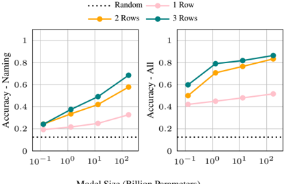
### Visual Description
\n
## Line Chart: Accuracy vs. Model Size
### Overview
The image presents two line charts comparing the accuracy of a naming task and an "All" task across different model sizes and numbers of rows. The x-axis represents model size in billions of parameters (logarithmic scale), and the y-axis represents accuracy. Each chart displays four data series, each representing a different number of rows (1, 2, 3) or a random baseline.
### Components/Axes
* **X-axis Label:** "Model Size (Billion Parameters)"
* **X-axis Scale:** Logarithmic, with markers at 10<sup>-1</sup>, 10<sup>0</sup>, and 10<sup>2</sup>.
* **Y-axis Label (Left Chart):** "Accuracy - Naming"
* **Y-axis Scale (Left Chart):** Linear, ranging from approximately 0.2 to 1.0.
* **Y-axis Label (Right Chart):** "Accuracy - All"
* **Y-axis Scale (Right Chart):** Linear, ranging from approximately 0.55 to 0.9.
* **Legend:** Located at the top-center of the image.
* "Random" - Black dotted line
* "1 Row" - Light pink solid line
* "2 Rows" - Orange solid line
* "3 Rows" - Teal solid line
### Detailed Analysis or Content Details
**Left Chart (Accuracy - Naming):**
* **Random (Black Dotted Line):** The line is relatively flat, starting at approximately 0.21 and ending at approximately 0.24.
* **1 Row (Light Pink Line):** The line slopes upward, starting at approximately 0.21 and ending at approximately 0.33.
* **2 Rows (Orange Line):** The line slopes upward more steeply than the "1 Row" line, starting at approximately 0.26 and ending at approximately 0.53.
* **3 Rows (Teal Line):** The line slopes upward even more steeply than the "2 Rows" line, starting at approximately 0.28 and ending at approximately 0.66.
**Right Chart (Accuracy - All):**
* **Random (Black Dotted Line):** The line is relatively flat, starting at approximately 0.58 and ending at approximately 0.61.
* **1 Row (Light Pink Line):** The line slopes upward gently, starting at approximately 0.58 and ending at approximately 0.68.
* **2 Rows (Orange Line):** The line slopes upward more steeply than the "1 Row" line, starting at approximately 0.55 and ending at approximately 0.82.
* **3 Rows (Teal Line):** The line slopes upward, starting at approximately 0.59 and ending at approximately 0.88.
### Key Observations
* In both charts, increasing the number of rows generally leads to higher accuracy.
* The "Random" baseline remains relatively constant across all model sizes, indicating it is not sensitive to model capacity.
* The "3 Rows" data series consistently achieves the highest accuracy in both charts.
* The difference in accuracy between the "1 Row" and "2 Rows" series is more pronounced than the difference between the "2 Rows" and "3 Rows" series, particularly in the "Accuracy - Naming" chart.
* The "Accuracy - All" chart shows a higher overall accuracy compared to the "Accuracy - Naming" chart.
### Interpretation
The data suggests that increasing the model size and the number of rows used in the model improves accuracy for both the naming task and the "All" task. The consistent performance of the "Random" baseline indicates that the observed improvements are due to the model's ability to learn from the data, rather than random chance. The diminishing returns observed when increasing from 2 to 3 rows suggest that there may be a point of saturation where adding more rows does not significantly improve performance. The higher accuracy in the "Accuracy - All" chart suggests that the model performs better when considering all available information, rather than focusing solely on naming. This could be due to the fact that the naming task is more challenging and requires more nuanced understanding of the data. The logarithmic scale on the x-axis indicates that the benefits of increasing model size may diminish as the model becomes larger. This is a common phenomenon in machine learning, as larger models can become more difficult to train and may not always generalize well to new data.
</details>
Model Size (Billion Parameters)
Figure 13: Macro average accuracy over all ImpartialRAVEN sub-tasks as we introduce rows to the matrix during in-context learning, under naming abstractions only (left) and all naming and decomposition abstractions (right). In 1 Row, we include only the incomplete third row.
## C Example Prompts
In Figure 14, we include example prompts for 2x2Grid , 3x3Grid , L-R and I-OG subtasks under different abstractions. Note that U-D and
I-OC are isomorphic to L-R , and therefore share the same prompt format.
<details>
<summary>Image 14 Details</summary>
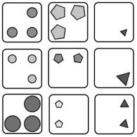
### Visual Description
\n
## Diagram: Shape Arrangement
### Overview
The image presents a 3x3 grid of square boxes. Each box contains a different arrangement of geometric shapes: circles, pentagons, hexagons, and triangles. The shapes vary in size and shade within each box. This appears to be a visual pattern or puzzle, rather than a data-driven chart.
### Components/Axes
There are no explicit axes or labels. The structure is defined by the 3x3 grid. The components are the individual boxes and the shapes within them.
### Detailed Analysis or Content Details
The grid can be described as follows, row by row:
* **Row 1:**
* Box 1: Contains three dark gray circles of approximately equal size.
* Box 2: Contains three light gray pentagons of approximately equal size.
* Box 3: Contains one black triangle pointing downwards.
* **Row 2:**
* Box 4: Contains three light gray circles of approximately equal size.
* Box 5: Contains two dark gray hexagons of approximately equal size.
* Box 6: Contains one black triangle pointing downwards.
* **Row 3:**
* Box 7: Contains two dark gray circles, one larger than the other.
* Box 8: Contains two light gray hexagons of approximately equal size.
* Box 9: Contains two black triangles pointing downwards.
### Key Observations
* Each row contains one box with triangles.
* The number of shapes varies between boxes.
* The shapes are consistently either dark gray, light gray, or black.
* The arrangement doesn't appear to follow a simple arithmetic or geometric progression.
### Interpretation
The image likely represents a visual reasoning puzzle or a pattern recognition task. The goal might be to identify the missing element in a sequence, or to determine the rule governing the arrangement of shapes. The variations in shape, size, and shade suggest that these factors are all relevant to the underlying pattern. Without further context, it's difficult to determine the specific logic or purpose of the arrangement. It could be a test of visual discrimination, spatial reasoning, or abstract thinking. The image does not provide any quantitative data or trends; it is purely a visual arrangement of shapes.
</details>
## 2x2Grid
<details>
<summary>Image 15 Details</summary>
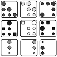
### Visual Description
\n
## Image: Arrangement of Geometric Shapes
### Overview
The image presents a 3x3 grid of square frames, each containing a varying arrangement of geometric shapes. The shapes include circles, squares, hexagons, and diamonds, with varying shades of gray and black. There are no explicit labels, axes, or legends. The image appears to be a visual pattern or a set of examples for a classification or matching task.
### Components/Axes
There are no axes or legends present in the image. The components are the nine square frames and the geometric shapes within them. Each frame is equally sized and arranged in a grid.
### Detailed Analysis or Content Details
The image consists of nine distinct arrangements of geometric shapes. Here's a breakdown of each frame, starting from the top-left and proceeding row by row:
* **Frame 1 (Top-Left):** Contains 5 hexagons (3 dark gray, 2 light gray) and 2 squares (both dark gray).
* **Frame 2 (Top-Center):** Contains 3 hexagons (1 dark gray, 2 light gray), 2 squares (both light gray), and 1 circle (light gray).
* **Frame 3 (Top-Right):** Contains 6 hexagons (all dark gray) and 1 circle (dark gray).
* **Frame 4 (Middle-Left):** Contains 1 large circle (dark gray), 2 squares (both dark gray), 1 hexagon (dark gray), and 2 smaller circles (both dark gray).
* **Frame 5 (Middle-Center):** Contains 2 squares (both light gray), 2 circles (both light gray), and 1 hexagon (light gray).
* **Frame 6 (Middle-Right):** Contains 3 squares (all dark gray) and 2 circles (both dark gray).
* **Frame 7 (Bottom-Left):** Contains 1 hexagon (light gray), 1 diamond (light gray), and 1 square (light gray), arranged vertically.
* **Frame 8 (Bottom-Center):** Contains 1 hexagon (light gray), 1 diamond (light gray), and 1 square (light gray), arranged vertically.
* **Frame 9 (Bottom-Right):** Contains 1 square (dark gray), 1 hexagon (dark gray), and 1 diamond (dark gray), arranged vertically.
### Key Observations
* The shapes vary in size and shade.
* The arrangements appear to be non-random, but there is no immediately obvious pattern governing their composition.
* Frames 7 and 8 are identical in shape and arrangement, differing only in shade.
* The number of shapes within each frame varies.
* There is a mix of shapes within each frame, with no frame containing only one type of shape.
### Interpretation
The image likely serves as a visual test or example set. It could be used for:
* **Pattern Recognition:** Identifying similarities and differences between the arrangements.
* **Classification:** Categorizing the frames based on their shape composition.
* **Visual Reasoning:** Determining the rules or principles governing the arrangement of shapes.
* **Abstract Thinking:** Exploring the relationships between geometric forms.
The repetition of Frame 7 and 8 suggests a possible element of redundancy or a deliberate inclusion of identical examples. The varying shades of gray might indicate a hierarchical relationship or a coding scheme. Without further context, it is difficult to determine the precise purpose of the image. It is a set of visual stimuli, but lacks the data to perform a quantitative analysis.
</details>
3x3Grid
<details>
<summary>Image 16 Details</summary>
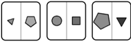
### Visual Description
Icon/Small Image (189x61)
</details>
<details>
<summary>Image 17 Details</summary>
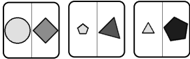
### Visual Description
Icon/Small Image (190x59)
</details>
<details>
<summary>Image 18 Details</summary>
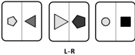
### Visual Description
\n
## Diagram: Shape Sequence
### Overview
The image presents a sequence of three rectangular frames, each containing two geometric shapes. The shapes vary in type (hexagon, triangle, pentagon, circle, square) and fill color (light gray, dark gray, black, white). A label "L-R" is positioned below the frames, indicating a left-to-right reading order.
### Components/Axes
The diagram consists of three distinct frames arranged horizontally. Each frame contains two shapes. There are no explicit axes or scales. The label "L-R" indicates the intended reading direction.
### Detailed Analysis or Content Details
**Frame 1 (Left):**
* Shape 1: Hexagon, light gray fill.
* Shape 2: Triangle pointing right, dark gray fill.
**Frame 2 (Center):**
* Shape 1: Triangle pointing right, light gray fill.
* Shape 2: Pentagon, dark gray fill.
**Frame 3 (Right):**
* Shape 1: Circle, light gray fill.
* Shape 2: Square, black fill.
### Key Observations
The diagram presents a sequence of shape pairs. The fill color alternates between light gray and dark gray within the first two frames. The final frame introduces a black-filled square. The shapes themselves change with each frame.
### Interpretation
The diagram appears to illustrate a progression or transformation of shapes and colors. The "L-R" label suggests a sequential order. The change in shapes and the introduction of a black square in the final frame could represent a shift in state or a final outcome. Without further context, the specific meaning of this sequence is unclear. It could be a visual representation of a process, a coding scheme, or a simple pattern recognition exercise. The diagram does not provide any quantitative data; it is purely qualitative. It is possible that the shapes represent different categories or states, and the color indicates a property or status associated with each.
</details>
<details>
<summary>Image 19 Details</summary>
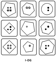
### Visual Description
\n
## Diagram: Geometric Shapes with Dots
### Overview
The image presents a 3x3 grid of geometric shapes, each containing a varying number of black dots. The shapes are contained within square frames. There are no axes, legends, or numerical data associated with the image. It appears to be a visual pattern or a test of visual discrimination.
### Components/Axes
There are no axes or legends. The components are:
* **Shapes:** Hexagon, Pentagon, Diamond, Square, Circle.
* **Dots:** Varying numbers of black dots (1 to 5) are placed within each shape.
* **Grid:** A 3x3 arrangement of the shapes.
* **Label:** "I-OG" is present in the bottom-right corner.
### Detailed Analysis or Content Details
The shapes and dot arrangements are as follows (row by row):
* **Row 1:**
* Hexagon with 4 dots.
* Hexagon with 2 dots.
* Circle with 2 dots.
* **Row 2:**
* Diamond with 4 dots.
* Hexagon with 1 dot.
* Hexagon with 2 dots.
* **Row 3:**
* Square with 5 dots.
* Pentagon with 1 dot.
* Hexagon with 3 dots.
### Key Observations
The image does not contain quantifiable data. The key observation is the variation in both shape and the number of dots within each shape. There is no apparent systematic ordering or progression in either the shapes or the dot counts.
### Interpretation
The image likely serves as a visual puzzle, a pattern recognition test, or a component of an intelligence assessment. The "I-OG" label could be an identifier for the test or a specific item within a larger set. Without further context, it's difficult to determine the purpose of the image. The arrangement appears random, suggesting the task might involve identifying anomalies, completing a pattern, or memorizing the configurations. The varying number of dots and shapes could be used to assess attention to detail, visual memory, or abstract reasoning skills. The image does not provide any factual data or demonstrate a specific relationship between the elements beyond their visual co-occurrence.
</details>
## Position: Prog.
row 1: [1, 0, 0, 1, 1, 0, 1, 1, 1], [1, 1, 0, 0, 1, 1, 0, 1, 1], [1, 1, 1, 0, 0, 1, 1, 0, 1];
row 2: [0, 1, 0, 1, 1, 0, 1, 1, 1], [1, 0, 1, 0, 1, 1, 0, 1, 1], [1, 1, 0, 1, 0, 1, 1, 0, 1];
row 3: [0, 1, 0, 0, 1, 0, 0, 1, 0], [0, 0, 1, 0, 0, 1, 0, 0, 1], [1, 0, 0, 1, 0, 0, 1, 0, 0];
## Type: Const.
## Size: Const.
## Number: -
row 1: 6, 6, 6;
row 2: 6, 6, 6;
row 3: 3, 3, 3;
## Color: Arith.
row 1: [5, 6], [5, 6], [5, 6];
row 1: [3, 4, 5, 6], [3, 4, 5, 6], [3, 4, 5, 6];
row 1: [6], [1], [7];
row 2: [4, 5, 6, 7], [4, 5, 6, 7], [4, 5, 6, 7];
row 2: [2, 3, 5], [2, 3, 5], [2, 3, 5];
row 2: [8], [0], [8];
row 3: [4, 5], [4, 5], [4, 5];
row 3: [1, 4, 5], [1, 4, 5], [1, 4, 5];
row 3: [4], [3], [7];
## Complete
row 1: A (3,0.1,40) / B (5,0.3,30), A (7,0.2,40) / B (4,0.3,50), A (5,0.6,40) / B (3,0.3,70);
row 2: A (7,0.6,10) / B (4,0.6,40), A (5,0.1,10) / B (3,0.6,60), A (3,0.2,10) / B (5,0.6,80);
row 3: A (5,0.2,10) / B (3,0.4,50), A (3,0.6,10) / B (5,0.4,70), A (7,0.1,10) / B (4,0.4,90);
## Left Comp.
## Right Comp.
row 1: (3,0.1,40), (7,0.2,40), (5,0.6,40);
row 1: (5,0.3,30), (4,0.3,50), (3,0.3,70);
row 2: (7,0.6,10), (5,0.1,10), (3,0.2,10);
row 2: (4,0.6,40), (3,0.6,60), (5,0.6,80);
row 3: (5,0.2,10), (3,0.6,10), (7,0.1,10);
row 3: (3,0.4,50), (5,0.4,70), (4,0.4,90);
| Type: Distr. | Size: Distr. | Color: Const. | Type: Distr. | Size: Const. | Color: Prog. |
|-----------------|-----------------|-----------------|-----------------|-----------------|-----------------|
| row 1: 3, 7, 5; | row 1: 1, 2, 6; | row 1: 4, 4, 4; | row 1: 5, 4, 3; | row 1: 3, 3, 3; | row 1: 3, 5, 7; |
| row 2: 7, 5, 3; | row 2: 6, 1, 2; | row 2: 1, 1, 1; | row 2: 4, 3, 5; | row 2: 6, 6, 6; | row 2: 4, 6, 8; |
| row 3: 5, 3, 7; | row 3: 2, 6, 1; | row 3: 1, 1, 1; | row 3: 3, 5, 4; | row 3: 4, 4, 4; | row 3: 5, 7, 9; |
## Complete
row 1: A (5,0.6,0) / B [(4,0.4,60), (4,0.4,60), (4,0.6,60), (4,0.6,60)],
A (6,0.5,0) / B [(6,0.6,30), (6,0.6,30), -, -],
A (7,0.4,0) / B [-, (5,0.5,90), -, (5,0.4,90)];
row 2: A (4,0.4,0) / B [-, (5,0.5,80), (5,0.3,80), (5,0.3,80)],
A (5,0.6,0) / B [(4,0.4,10), -, -, -],
A (6,0.5,0) / B [-, (6,0.5,90), (6,0.3,90), -];
row 3: A (4,0.5,0) / B [(6,0.4,40), (6,0.4,40), (6,0.4,40), (6,0.3,40)],
A (5,0.4,0) / B [-, (5,0.5,50), -, -],
A (6,0.6,0) / B [(4,0.4,90), (4,0.4,90), (4,0.5,90), -];
## In Comp.
row 1: [(4,0.4,60), (4,0.4,60), (4,0.6,60), (4,0.6,60)],
[(6,0.6,30), (6,0.6,30), -, -],
[-, (5,0.5,90), -, (5,0.4,90)];
row 2: [-, (5,0.5,80), (5,0.3,80), (5,0.3,80)],
[(4,0.4,10), -, -, -],
[-, (6,0.5,90), (6,0.3,90), -];
row 3: [(6,0.4,40), (6,0.4,40), (6,0.4,40), (6,0.3,40)],
[-, (5,0.5,50), -, -],
[(4,0.4,90), (4,0.4,90), (4,0.5,90), -];
## Position: -
## Number: Arith.
row 1: [1, 1, 1, 1], [1, 1, 0, 0], [0, 1, 0, 1];
row 2: [0, 1, 1, 1], [1, 0, 0, 0], [0, 1, 1, 0];
row 3: [1, 1, 1, 1], [0, 1, 0, 0], [1, 1, 1, 0];
row 1: 4, 2, 2;
row 2: 3, 1, 2;
row 3: 4, 1, 3;
## Type: Distr.
Size: Const.
## Color: Arith.
row 1: [4], [6], [5]; row 1: [4, 6], [6], [4, 5]; row 1: [6], [3], [9];
row 2: [5], [4], [6]; row 2: [3, 5], [4], [3, 5]; row 2: [8], [1], [9];
row 3: [6], [5], [4]; row 3: [3, 4], [5], [4, 5]; row 3: [4], [5], [9];
Figure 14: Example prompts for 2x2Grid , 3x3Grid , L-R and I-OG subtasks under different abstractions.
## Out Comp.
row 1: (5,0.6,0), (6,0.5,0), (7,0.4,0);
row 2: (4,0.4,0), (5,0.6,0), (6,0.5,0);
row 3: (4,0.5,0), (5,0.4,0), (6,0.6,0);
Type: Prog. Size: Distr. Color: Const.
row 1: 5, 6, 7; row 1: 6, 5, 4; row 1: 0, 0, 0;
row 2: 4, 5, 6;
row 2: 4, 6, 5;
row 2: 0, 0, 0;
row 3: 4, 5, 6; row 3: 5, 4, 6; row 3: 0, 0, 0;
## Complete
row 1: [-, (7,0.2,40), (7,0.2,40), (7,0.2,40)], [(5,0.5,20), (5,0.5,20), (5,0.5,20), -], [-, -, -, (3,0.1,60)];
row 2: [(7,0.1,20), (7,0.1,20), -, (7,0.1,20)], [(5,0.2,40), (5,0.2,40), -, -], [-, -, -, (3,0.5,60)];
row 3: [-, (7,0.5,50), (7,0.5,50), (7,0.5,50)], [(5,0.1,10), -, (5,0.1,10), -], [-, (3,0.2,60), -, (3,0.2,60)];
## Position: (Set) Arith.
## Number: -
## Type: Prog.
## Size: Distr.
## Color: Arith.
row 1: [0, 1, 1, 1], [1, 1, 1, 0], [0, 0, 0, 1];
row 1: 3, 3, 1;
row 1: [7], [5], [3];
row 1: [2], [5], [1];
row 1: [4], [2], [6];
row 2: [1, 1, 0, 1], [1, 1, 0, 0], [0, 0, 0, 1];
row 2: 3, 2, 1;
row 2: [7], [5], [3];
row 2: [1], [2], [5];
row 2: [2], [4], [6];
row 3: [0, 1, 1, 1], [1, 0, 1, 0], [0, 1, 0, 1];
row 3: 3, 2, 2;
row 3: [7], [5], [3];
row 3: [5], [1], [2];
row 3: [5], [1], [6];
## Complete
row 1: [(5,0.6,60), -, -, (6,0.4,60), (6,0.5,60), -, (5,0.3,60), (6,0.3,60), (6,0.4,60)],
[(6,0.4,10), (5,0.6,10), -, -, (6,0.4,10), (6,0.5,10), -, (5,0.3,10), (6,0.3,10)],
[(6,0.3,70), (6,0.4,70), (5,0.6,70), -, -, (6,0.4,70), (6,0.5,70), -, (5,0.3,70)];
row 2: [-, (7,0.5,80), -, (4,0.3,80), (7,0.2,80), -, (6,0.2,80), (5,0.3,80), (4,0.5,80)],
[(4,0.5,0), -, (7,0.5,0), -, (4,0.3,0), (7,0.2,0), -, (6,0.2,0), (5,0.3,0)],
[(5,0.3,80), (4,0.5,80), -, (7,0.5,80), -, (4,0.3,80), (7,0.2,80), -, (6,0.2,80)];
row 3: [-, (5,0.5,40), -, -, (4,0.4,40), -, -, (4,0.1,40), -],
[-, -, (5,0.5,30), -, -, (4,0.4,30), -, -, (4,0.1,30)],
[(4,0.1,70), -, -, (5,0.5,70), -, -, (4,0.4,70), -, -];
Table 3: Performance on RAVEN sub-tasks under our abstractions across a wider set of model sizes. 175B refers to text-davinci-002 while the rest are corresponding OPT models.
| Abstractions | Center | 2x2 | 3x3 | L-R | U-D | O-IC | O-IG | Avg. |
|-----------------------|----------|-------|-------|-------|-------|--------|--------|--------|
| Attr. Naming Only | 0.222 | 0.42 | 0.606 | 0.076 | 0.098 | 0.122 | 0.194 | 0.248 |
| Comp. Decomp. | 0.222 | 0.42 | 0.606 | 0.136 | 0.154 | 0.162 | 0.222 | 0.275 |
| Comp. + Attr. Decomp. | 0.456 | 0.62 | 0.724 | 0.378 | 0.408 | 0.374 | 0.52 | 0.497 |
| Attr. Naming Only | 0.302 | 0.51 | 0.684 | 0.104 | 0.134 | 0.12 | 0.25 | 0.301 |
| Comp. Decomp. | 0.302 | 0.51 | 0.684 | 0.186 | 0.232 | 0.254 | 0.344 | 0.359 |
| Comp. + Attr. Decomp. | 0.436 | 0.588 | 0.788 | 0.28 | 0.346 | 0.29 | 0.408 | 0.448 |
| Attr. Naming Only | 0.472 | 0.584 | 0.71 | 0.146 | 0.158 | 0.2 | 0.322 | 0.37 |
| Comp. Decomp. | 0.472 | 0.584 | 0.71 | 0.41 | 0.426 | 0.434 | 0.494 | 0.504 |
| Comp. + Attr. Decomp. | 0.72 | 0.714 | 0.794 | 0.672 | 0.68 | 0.744 | 0.744 | 0.724 |
| Attr. Naming Only | 0.534 | 0.572 | 0.746 | 0.216 | 0.2 | 0.268 | 0.336 | 0.41 |
| Comp. Decomp. | 0.534 | 0.572 | 0.746 | 0.42 | 0.468 | 0.484 | 0.532 | 0.537 |
| Comp. + Attr. Decomp. | 0.706 | 0.738 | 0.826 | 0.658 | 0.664 | 0.704 | 0.784 | 0.726 |
| Attr. Naming Only | 0.618 | 0.59 | 0.752 | 0.196 | 0.228 | 0.284 | 0.396 | 0.438 |
| Comp. Decomp. | 0.618 | 0.59 | 0.752 | 0.492 | 0.528 | 0.548 | 0.584 | 0.587 |
| Comp. + Attr. Decomp. | 0.704 | 0.75 | 0.826 | 0.682 | 0.69 | 0.748 | 0.834 | 0.748 |
| Attr. Naming Only | 0.644 | 0.61 | 0.754 | 0.22 | 0.268 | 0.358 | 0.452 | 0.472 |
| Comp. Decomp. | 0.644 | 0.61 | 0.754 | 0.566 | 0.602 | 0.586 | 0.576 | 0.62 |
| Comp. + Attr. Decomp. | 0.746 | 0.794 | 0.83 | 0.71 | 0.702 | 0.77 | 0.84 | 0.77 |
| Attr. Naming Only | 0.68 | 0.596 | 0.748 | 0.264 | 0.328 | 0.42 | 0.482 | 0.503 |
| Comp. Decomp. | 0.68 | 0.596 | 0.748 | 0.582 | 0.618 | 0.664 | 0.638 | 0.647 |
| Comp. + Attr. Decomp. | 0.762 | 0.818 | 0.828 | 0.738 | 0.714 | 0.786 | 0.86 | 0.787 |
| Attr. Naming Only | 0.772 | 0.78 | 0.864 | 0.542 | 0.536 | 0.648 | 0.748 | 0.699 |
| Comp. Decomp. | 0.772 | 0.78 | 0.864 | 0.738 | 0.732 | 0.78 | 0.84 | 0.787 |
| Comp. + Attr. Decomp. | 0.8 | 0.878 | 0.932 | 0.776 | 0.78 | 0.828 | 0.926 | 0.846 |
Table 4: Performance on I-RAVEN sub-tasks under our abstractions across different model sizes. 175B refers to text-davinci-002 while the rest are corresponding OPT models.
| Abstractions | Abstractions | Center | 2x2 | 3x3 | L-R | U-D | O-IC | O-IG | Avg. |
|----------------|-----------------------|----------|-------|-------|-------|-------|--------|--------|--------|
| | Attr. Naming Only | 0.376 | 0.172 | 0.208 | 0.246 | 0.23 | 0.262 | 0.202 | 0.242 |
| 125M | Comp. Decomp. | 0.376 | 0.172 | 0.208 | 0.336 | 0.344 | 0.354 | 0.224 | 0.288 |
| | Comp. + Attr. Decomp. | 0.608 | 0.514 | 0.602 | 0.612 | 0.624 | 0.638 | 0.594 | 0.6 |
| 1.3B | Attr. Naming Only | 0.594 | 0.29 | 0.31 | 0.348 | 0.37 | 0.388 | 0.334 | 0.376 |
| | Comp. Decomp. | 0.594 | 0.29 | 0.31 | 0.586 | 0.574 | 0.618 | 0.466 | 0.491 |
| | Comp. + Attr. Decomp. | 0.81 | 0.676 | 0.73 | 0.822 | 0.802 | 0.882 | 0.818 | 0.791 |
| 13B | Attr. Naming Only | 0.756 | 0.384 | 0.382 | 0.456 | 0.498 | 0.538 | 0.432 | 0.492 |
| | Comp. Decomp. | 0.756 | 0.384 | 0.382 | 0.75 | 0.74 | 0.766 | 0.564 | 0.62 |
| | Comp. + Attr. Decomp. | 0.836 | 0.748 | 0.728 | 0.824 | 0.826 | 0.906 | 0.868 | 0.819 |
| | Attr. Naming Only | 0.808 | 0.564 | 0.566 | 0.656 | 0.676 | 0.818 | 0.714 | 0.686 |
| 175B | Comp. Decomp. | 0.808 | 0.564 | 0.566 | 0.822 | 0.812 | 0.896 | 0.742 | 0.744 |
| 175B | Comp. + Attr. Decomp. | 0.864 | 0.832 | 0.818 | 0.834 | 0.846 | 0.928 | 0.93 | 0.865 |