2306.00107v5

# MERT: Acoustic Music Understanding Model with Large-Scale Self-supervised Training > The authors contributed equally to this work. Corresponding authors. ## Abstract Self-supervised learning (SSL) has recently emerged as a promising paradigm for training generalisable models on large-scale data in the fields of vision, text, and speech. Although SSL has been proven effective in speech and audio, its application to music audio has yet to be thoroughly explored. This is partially due to the distinctive challenges associated with modelling musical knowledge, particularly tonal and pitched characteristics of music. To address this research gap, we propose an acoustic M usic und ER standing model with large-scale self-supervised T raining (MERT), which incorporates teacher models to provide pseudo labels in the masked language modelling (MLM) style acoustic pre-training. In our exploration, we identified an effective combination of teacher models, which outperforms conventional speech and audio approaches in terms of performance. This combination includes an acoustic teacher based on Residual Vector Quantisation - Variational AutoEncoder (RVQ-VAE) and a musical teacher based on the Constant-Q Transform (CQT). Furthermore, we explore a wide range of settings to overcome the instability in acoustic language model pre-training, which allows our designed paradigm to scale from 95M to 330M parameters. Experimental results indicate that our model can generalise and perform well on 14 music understanding tasks and attain state-of-the-art (SOTA) overall scores. The code and models are online: https://github.com/yizhilll/MERT. ## 1 Introduction Pre-trained language models (PLMs) can learn generalisable representations of data without human annotated labels in a self-supervised learning (SSL) style, leading to remarkable performance improvement in natural language processing and related fields (Brown et al.,, 2020; Fang et al.,, 2022; Chen et al., 2021a, ). Music is widely recognised as a special language that can be used to communicate across different cultures (Mehr et al.,, 2019). The internal similarity between music and language as a communication interface lays a promising foundation for adapting PLM-based methods to model music sequences. We argue that the benefit is twofold. First, PLMs can potentially pave the way to unify the modelling of a wide range of music understanding, or the so-called Music Information Retrieval (MIR) tasks, including but not limited to music tagging, beat tracking, music transcription, and source separation, so that different tasks no longer need task-specific models or features. Second, releasing a PLM for acoustic music understanding allows the redistribution of the musical knowledge rather than the data itself, which saves the costs of manual annotation and copyright law restrictions. Unfortunately, we are yet to see a general-purpose and cost-effective open-source PLM on acoustic music understanding. Most existing studies are designed to solely address music tagging problems (Pons and Serra,, 2019; Spijkervet and Burgoyne,, 2021; McCallum et al.,, 2022; Huang et al.,, 2022; Zhu et al.,, 2021; Zhao and Guo,, 2021), and many of them do not provide open-source code bases or checkpoints for further evaluation. A promising model is JukeMIR (Castellon et al.,, 2021), which is based on Jukebox (Dhariwal et al.,, 2020) and provides a comprehensive evaluation on MIR downstream tasks. However, this foundation model uses cumbersome hierarchical auto-regressive transformer decoders containing billions of parameters to model music audio, leading to significant inefficiency for conducting general music understanding tasks (e.g., it takes weeks to carry out inference on datasets like MTG (Bogdanov et al.,, 2019) with a consumer-grade 3090 GPU). <details> <summary>x14.png Details</summary>  ### Visual Description ## Diagram: Audio Processing System with Dual MLMs and Transformer Encoder ### Overview The diagram illustrates a multi-modal audio processing system that integrates acoustic and musical features using two separate Masked Language Models (MLMs) and a Transformer Encoder. The system processes raw audio waveforms through a 1D convolution feature extractor, generates contextual representations, and employs teacher-student learning for both acoustic and musical domains. ### Components/Axes 1. **Input Path**: - **Audio Waveform**: Raw audio signal (x₁–x₄) with labeled segments (G, E, m, C, D, B, 7, Am, 7). - **1D Convolution Feature Extractor**: Converts audio waveforms into masked audio features. 2. **Core Processing**: - **Transformer Encoder**: Processes masked audio features to produce contextual representations (z₁–z₄). - **Acoustic MLM**: Receives contextual representations (z₁–z₄) and input from the Acoustic Teacher (VQ(x₂), VQ(x₃)). - **Musical MLM**: Receives contextual representations (z₁–z₄) and input from the Musical Teacher (CQT(x₂), CQT(x₃)). 3. **Teachers**: - **Acoustic Teacher**: Provides VQ(x₂), VQ(x₃) to the Acoustic MLM. - **Musical Teacher**: Provides CQT(x₂), CQT(x₃) to the Musical MLM. ### Detailed Analysis - **Audio Waveform**: The input signal is segmented into labeled regions (e.g., "G," "E," "m," "C," "D," "B," "Am," "7"), suggesting a focus on musical notation or phonetic analysis. - **Feature Extraction**: The 1D convolution layer extracts masked audio features, likely emphasizing temporal patterns while suppressing certain frequencies or time intervals. - **Transformer Encoder**: Generates four contextual representations (z₁–z₄), which serve as shared inputs for both MLMs. - **Dual MLMs**: - The **Acoustic MLM** integrates acoustic features (VQ(x₂), VQ(x₃)) with contextual representations. - The **Musical MLM** integrates musical features (CQT(x₂), CQT(x₃)) with contextual representations. - **Teachers**: The Acoustic and Musical Teachers act as auxiliary models, providing domain-specific guidance (e.g., VQ for vector quantization, CQT for chroma-based features). ### Key Observations 1. **Modular Design**: The system separates acoustic and musical processing streams while sharing contextual representations, enabling cross-modal learning. 2. **Teacher-Student Dynamics**: The teachers likely refine the MLMs through contrastive learning or knowledge distillation, improving generalization. 3. **Masked Features**: The use of masked audio features suggests a self-supervised learning approach, similar to BERT for audio. ### Interpretation This architecture demonstrates a hybrid approach to audio understanding, combining: - **Acoustic Analysis**: Focused on raw sound properties (e.g., timbre, amplitude). - **Musical Context**: Leveraging chroma features (CQT) for pitch and harmony recognition. - **Transformer-Based Context**: Capturing long-range dependencies in audio sequences. The dual MLM design allows the system to handle tasks requiring both sound-level and music-level understanding, such as: - Music transcription (converting audio to sheet music). - Emotion recognition in music. - Speech-to-music generation. The teachers’ roles highlight the importance of domain-specific priors in improving model robustness. For example, the Acoustic Teacher might enforce consistency in low-level features, while the Musical Teacher ensures alignment with harmonic structures. 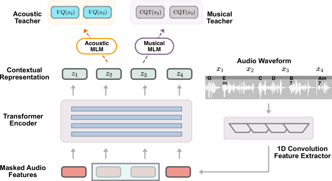</details> Figure 1: Illustration of the MERT Pre-training Framework. The aforementioned research gap has urged us to design and open-source a generalisable and computationally affordable pre-trained acoustic music model. In this paper, we propose an acoustic M usic und ER standing model with large-scale self-supervised T raining (MERT). MERT inherits a speech SSL paradigm, employing teacher models to generate pseudo targets for sequential audio clips. Specifically, to capture the distinctive pitched and tonal characteristics in music, MERT incorporates a multi-task paradigm to balance the acoustic and musical representation learning as demonstrated in Fig. 1. In the proposed design, a Residual Vector Quantisation - Variational Autoencoder (RVQ-VAE) (Défossez et al.,, 2022) is used as the acoustic teacher to provide discretised acoustic-level summarisation of the music signal. The Constant-Q Transformation (CQT) (Brown,, 1991) model is further introduced as the music teacher for capturing pitch and harmonic inductive bias. Regarding the context dependencies and music hierarchies, as indicated in Borsos et al., (2022), we leave the task of modelling high-level and abstract patterns to the stacked layers of self-attentions in the transformer. We also explore a wide range of settings for the transformer and 1D convolution encoder to overcome the instability in acoustic model pre-training, which permits effective scaling up of MERT from 95M to 330M size when blending acoustic and musical knowledge. By scaling up to 330M size (only 7% the size of JukeBox), MERT achieves overall state-of-the-art (SOTA) results on various MIR tasks, which demonstrates a strong generalisability on music understanding. Last but not least, we analyse multiple pre-trained settings considering the teachers and share our decision routes § 5.2 and § 5.3, which could potentially guide future acoustic music understanding pre-training research. To summarise, our contributions are: - proposing a multi-task style predictive acoustic self-supervised learning paradigm, which achieves SOTA performance on various MIR tasks, including important yet unexplored tasks for pre-training such as pitch detection, beat tracking and source separation applications; - conducting a broad range of analysis based on ablation studies of the proposed MERT pre-training paradigm; - exploring robust and stable strategies for acoustic music model training to overcome training instability and frequent crashes when scaling up the pre-training on model size; - providing an open-source, generalisable and computationally affordable acoustic music pre-trained model, which addresses the needs of both industry and research communities. ## 2 Related Work #### PLMs for Acoustic Music The field of music information retrieval (MIR) has long been facing challenges in data availability due to the costs associated with music audio annotation and country-specific copyright laws (Chen et al.,, 2019; Castellon et al.,, 2021). To address this challenge, pre-trained language models (PLMs) for acoustic music have been proposed to provide reusable learned representations, enabling transfer learning for various downstream MIR tasks without the need for extensive data annotation (Castellon et al.,, 2021). However, current acoustic music pre-trained models still have room for improvement in terms of providing open-source, generalisable, and lightweight learned representations suitable for both industrial and research applications (McCallum et al.,, 2022). Existing acoustic music pre-trained models primarily focus on tagging tasks and rely on supervised tagging labels for pre-training (Pons and Serra,, 2019; Spijkervet and Burgoyne,, 2021; McCallum et al.,, 2022; Huang et al.,, 2022). While some studies have explored contrastive learning for acoustic music pre-training, they face limitations in training data and model size, hampering the performance improvements (Choi et al.,, 2017; Li et al.,, 2022). Additionally, several models trained on inaccessible datasets or without publicly available codes and model weights make it difficult to reproduce or extend their approaches (McCallum et al.,, 2022; Castellon et al.,, 2021; Li et al.,, 2022; Zhu et al.,, 2021; Zhao and Guo,, 2021). Although some general-purpose audio representation models show potential for music audio representation learning, their performance is mostly evaluated on limited MIR downstream tasks (Saeed et al.,, 2021; Borsos et al.,, 2022; Wang et al.,, 2023). This lack of comprehensive evaluation hinders further studies and a thorough understanding of the pros and cons of existing models. #### Self-Supervised Speech Processing Music and speech processing are closely related (Jasmin et al.,, 2020) since they usually use the same audio data formats. Additionally, both acoustic music and speech processing models need to deal with the cocktail party problem (Brown and Bidelman,, 2022; Petermann et al.,, 2022) since good source separation capabilities help both separating noises and background sounds with speech and processing polyphonic music audio. These common grounds between music and speech processing inspire us to adapt SOTA speech pre-trained models and tailor them specifically for music audio processing tasks. For instance, existing research work targeting general-purpose audio representations (Saeed et al.,, 2021; Borsos et al.,, 2022; Wang et al.,, 2023) has verified that self-supervised speech processing models can be extended beyond speech to downstream entry-level music tasks, including generating mono piano music and music reconstruction. #### Audio Representation with Language Modelling Mask strategy-based large-scale language models have been applied to a wide range of domains (Lample and Charton,, 2019; Chen et al., 2021a, ; Chen et al., 2021b, ; Fang et al.,, 2022), but still remain under-explored in acoustic music understanding. For audio, Dhariwal et al., (2020) investigates generating hierarchical tokens which can be further employed to reconstruct music, inspiring subsequent research to understand and generate acoustic music based on extracted discrete tokens from continuous features. Baevski and Mohamed, (2020) introduce a pre-trained VQ-VAE (Baevski et al.,, 2019) to provide prediction targets to conduct speech representation learning with MLM. While introducing K-means to provide discrete token codebooks and pre-training the model to detect sound units, Hsu et al., (2021) claim that a better teacher model in SSL could lead to better downstream task performance. Additionally, recent speech processing pre-trained models (Borsos et al.,, 2022; Wang et al.,, 2023) propose to train or adopt separately trained codecs (Zeghidour et al.,, 2021; Défossez et al.,, 2022) for discrete token extraction. Based on the conclusion from previous studies, the recently released RVQ-VAEs (Zeghidour et al.,, 2021; Défossez et al.,, 2022), achieving good results in music reconstruction, could be adopted as teacher models for music understanding pre-training and provide acoustic information guidance. Yet some of the uniqueness of music processing such as timbre and harmony remains unexplored. We thus propose to incorporate a corresponding musical teacher model in MERT to fill such an important gap. ## 3 Methodology This section introduces the pre-training paradigm and architecture of our models. It includes prediction to acoustic teachers such as k-means or deep music features, and reconstruction to music teachers such as CQT spectrum, both based on the well-established masked language modelling (MLM). ### 3.1 Pre-training with MLM Supervised Learning requires a labelled dataset $D_t=\{x_i^(t),y_i^(t)\}^N_i=1$ . Here, $N$ is the number of data samples, $x_i^(t)$ is the $i^th$ data sample in the dataset, and $y_i^(t)$ is the corresponding label. From $D_t$ , we can train a machine learning algorithm $f_θ≤ft(·\right)$ parameterised with $θ$ that makes label predictions on each data sample. Unsupervised learning, in contrast, learns an algorithm based on an unlabelled dataset $D=\{x_i\}^M_i=1$ , with SSL being a specific type of this class. For each data sample $x_i$ , SSL derives a new data $x_i^\prime$ with a pseudo label $y_i^\prime$ . The training process is to minimise the loss between each pseudo label $y_i^\prime$ and the prediction based on new data $\hat{y}_i=f_θ(x_i^\prime)$ as denoted in Eq. 1. $$ θ^∗={arg min}_θ∑_x_{i^(t)∈ D}L≤ft(f_ θ(x_i^\prime(t)),y_i^\prime(t)\right). \tag{1} $$ MLM is a famous example of pseudo-label generation. Let $x_i=≤ft[x_i^(1),x_i^(2),⋯,x_i^(L)\right]$ be the $i^th$ data sample in a sequential dataset with length $L$ , and $M⊂[L]$ is a subset of indices randomly chosen from $1$ to $L$ . Then, the new data is defined by the following equation $$ x_i^\prime=≤ft[1_[L]∖ M(1)· x_i^(1),1 _[L]∖ M(2)· x_i^(2),⋯,1_[L]∖ M(L) · x_i^(L)\right] \tag{1} $$ where $1_[L]∖ M(x)$ denotes the indicator function, that is, $1_[L]∖ M(x)=1$ if and only if $x$ is outside the masked indices set $M$ . The pseudo-label that needs to be learned is typically $y_i^\prime=x_i-x_i^\prime$ , i.e., the masked data. However, reconstructing masked data $y^\prime$ for raw audio tasks as pseudo-labels is hard to train. HuBERT (Vaswani et al.,, 2017; Hsu et al.,, 2021) uses a dimension-reduced feature $z^\prime$ derived from $y^\prime$ with phonetic acoustic information, which forms the design basis of our pre-training strategy. As a speech SSL system, HuBERT utilises offline clustering to acquire pseudo labels for a BERT-like prediction loss. Specifically, it uses Mel-frequency cepstral coefficients (MFCCs), a widely-used traditional feature in speech-related tasks, as acoustic features for clustering. The obtained results are then utilised as pseudo labels in the first iteration of pre-training. It then uses the learned representation for clustering to get a pseudo label for the second iteration pre-training. Such a pseudo label includes acoustic information in human speech and can be aligned to phonemes. The loss functions of HuBERT are formulated as follows: $$ L_H(f;x,M,Z)=∑_t∈ M\log p_f(z_t\mid x^\prime,t) \tag{3} $$ where $\log p_f(·\mid x^\prime,t)$ is the log-likelihood function on clustering results given the masked input $x^\prime$ and position $t$ derived from $f$ ; likelihood function $p_f$ is the Noise Contrastive Estimation (NCE) loss which is defined as $$ p_f(c\mid x^\prime,t)=\frac{\exp(sim(T(o_t),e_c)/τ)}{∑_c ^\prime=1^C\exp(sim(T(o_t),e_c^\prime)/τ)}, \tag{4} $$ Here, $c∈[C]$ is a codeword of the clustering results and $e_c$ represents its embedding; sim is the cosine similarity; $o_t$ is the output of the model at timestep $t$ ; and $T(o_t)$ is the linear transformation of $o_t$ , making it have the same dimension as $e_c$ . Besides, $τ$ scales the logit which is set to $0.1$ in HuBERT. The linear transformation $T$ , the model to generate outputs, and the embedding of all the clustering results are all learnable. Overall, we use the same model as HuBERT but introduce several notable variations tailored to music. Specifically, we designed a better hidden-unit $z$ as pseudo tags for pre-training with multiple music acoustic features. In addition, we added a reconstruction loss to music features and employed additional music augmentation tricks. ### 3.2 Modelling Acoustic Information The MFCC features are only good at modelling acoustic and timbre information for single-pitch signals, and therefore, the clustering results do not provide much timbre information in music recordings. We proposed two potential approaches as the teacher on acoustic information: one based on traditional features, and the other based on deep learning. The first method uses k-means on the log-Mel spectrum and Chroma features for timbre and harmonic acoustic information, respectively. In the case of music representations, each frame contains more information compared to speech, necessitating a larger number of classes for k-means clustering. The complexity of the k-means algorithm is linear with the number of centroids (clustering centres), leading to a time-consuming k-means for the music feature. To tackle this problem, we employ 300-means for the log-Mel spectrum with dimension 229, and 200-means for Chroma features with dimension 264, resulting in a total of 60,000 classes (200 centroids for Chroma features multiplied by 300 centroids for the log-Mel spectrum). Despite the increased number of classes, the computational complexity remains comparable to that of HuBERT. The disadvantage of k-means is that it is difficult to scale up to a larger number of classes and larger datasets, and the results are sensitive to initialisation. The second choice for our acoustic teacher is EnCodec (Défossez et al.,, 2022), a recent learnable feature with 8-layer residual Vector Quantized-Variational AutoEncoder (VQ-VAE). Each acoustic feature, denoted as $z_enc∈[C]^L× 8$ , is a 2-dimensional auditory code matrix, and $L$ is the length of the recording. The row vector of each matrix $z_enc[t,:]$ represents the results of $8$ different clusterings for frame $t$ , and the column vector of each matrix $z_enc[:,j]$ represents the results from the $j^th$ codebook of the audio sequence, where $j∈\{1,…,8\}$ . EnCodec converts 24kHz input waveforms to 8 different embeddings at 75Hz with a 320-fold reduction, and the quantizer has $1024$ dimensions. In this setting, for each 5-second waveform, the discrete acoustic feature is a matrix with $375× 8$ entries, representing 375 frames (75Hz × 5s) and 8 deep acoustic features. With these embeddings, the decoder of EnCodec can reconstruct the waveform at 24 kHz with authentic information in timbre. ### 3.3 Modelling Musical Information Apart from acoustic information, we added a new reconstruction loss to the Constant-Q transform (CQT) spectrogram to emphasise pitch-level information. The CQT is a type of frequency transform that is widely used in various MIR tasks, such as pitch detection, chord recognition, and music transcription. It is similar to the Fourier transform, but bin widths are proportional to frequency rather than equal, giving each octave the same number of bins, resulting in a better time-frequency trade-off for music audio where multiple pitches occur in multiple octaves. We utilize mean squared error (MSE) loss to reconstruct the CQT spectrum $z_cqt$ from the masked input audio $x^\prime$ . That is, $$ L_CQT(f_cqt;x,M,z_cqt)=∑_t∈ M≤ft\|z_cqt,t- f_cqt(x^\prime)_t\right\|_2 \tag{5} $$ And the final loss function $L$ is a linear combination of both the acoustic loss function $L_H$ and the musical-pitch loss function $L_CQT$ : $$ L=α·L_H+L_CQT \tag{6} $$ ## 4 Experiments ### 4.1 Evaluation Protocol #### Downstream Tasks We evaluate our method and compare it with baseline models on 14 downstream tasks, including frame-level classification or regression tasks like music tagging, key detection, genre classification, emotion score regression, instrument classification, pitch classification, vocal technique detection, and singer identification; and sequential tasks like beat tracking and source separation. For instrument classification, we use the Nsynth (Engel et al.,, 2017) and MTG-instrument datasets, with receiver operating characteristic (ROC), and average precision (AP). The NSynth dataset is also used for pitch classification, with accuracy (ACC) as the evaluation metric. Vocal technique detection and singer identification based on the VocalSet dataset (Wilkins et al.,, 2018), with accuracy as the metric. For music tagging, we utilise the MagnaTagATune (MTT) (Law et al.,, 2009) and MTG-Jamendo (Bogdanov et al.,, 2019) datasets, averaging multiple embeddings for long audio recordings. Key detection is accomplished using the Giantsteps and Giantsteps-MTG-keys datasets (Knees et al.,, 2015; Korzeniowski and Widmer,, 2017), with a refined accuracy (ACC refined) metric. Genre classification is performed using the GTZAN (Tzanetakis and Cook,, 2002) and MTG-Genre datasets, with ROC, and AP metrics. Emotion score regression is conducted on the Emomusic dataset (Soleymani et al.,, 2013), with the coefficient of determination (R2 score) of arousal and valence as evaluation metrics. Beat tracking is conducted on the GTZAN Rhythm dataset (Marchand and Peeters,, 2015), using the F-measure (F1). Finally, source separation is accomplished using the MUSDB18 dataset (Rafii et al.,, 2017), with the Source-to-Distortion Ratio (SDR) as the evaluation metric. The full descriptions of the datasets and tasks can be found in Appendix B.1. #### Probing Protocol Following Castellon et al., (2021); Yang et al., (2021), we restrict the testing protocol with probing rather than fine-tuning, i.e. freezing the backbone pre-trained models as deep feature extractor and only train a simple downstream structure, typically a multilayer perceptron (MLP) for frame-level tasks. For a fair comparison, we also limit the space for hyper-parameter search. For full details please refer to Appendix B.2. ### 4.2 Baseline Methods We select models pre-trained with various paradigms from both music and speech domains as our baselines to provide a comprehensive evaluation of the generalisation ability of the designs. MusiCNN (Pons and Serra,, 2019) is selected as a representative supervised method, which is pre-trained with supervision from the Million Song Dataset tags (Bertin-Mahieux et al.,, 2011). CLMR (Spijkervet and Burgoyne,, 2021) and MULE (McCallum et al.,, 2022) are selected as representatives of SOTA music representations trained with contrastive learning. Jukebox (Dhariwal et al.,, 2020) and the corresponding transfer learning method, JukeMIR (Castellon et al.,, 2021) is selected as the representative of transfer learning from a large-scale generative pre-trained musical representation. We also select the recently proposed strong speech SSL models, HuBERT (Hsu et al.,, 2021) and data2vec (Baevski et al.,, 2022), as our baselines since they share the same MLM pre-training paradigm with MERT. While HuBERT reconstructs the masked discrete tokens provided by the K-means teacher, data2vec uses the student model updated with an exponential moving average gradient to produce continuous representations for MLM prediction. In order to reveal the effectiveness of the pre-training paradigm itself rather than the training data distribution, we re-train the speech models and denote them by HuBERT music and data2vec music. Additionally, we present the current SOTA for each task including results from both supervised and self-supervised methods. ### 4.3 Implementation Details #### Training Settings We deploy the proposed SSL architecture in the training of various model sizes with matched scales of data. We mined 160K hours of music recordings from the Internet to build a large-scale music dataset. Accordingly, the base size models (95M) are trained with a 1K hours subset whereas the whole dataset is used for the large model (330M). Specifically, we provide a special edition of the base model, MERT-95M-public, that is trained on a totally publicly available music dataset, music4all (Santana et al.,, 2020), with a data size of 910 hours. In the context of self-attention, the computational complexity scales quadratically with the sequence length. Therefore, when dealing with limited computational resources, there exists a trade-off between the batch size and the sequence length. In our preliminary experiments, we have observed that increasing the batch size provides greater performance improvements compared to extending the context length. To allow a larger batch size under the computational limitation, we adopt a strategy of randomly truncating audio clips into 5-second segments following Ma et al., (2023). This duration roughly corresponds to a 2-bar context in music. It is worth noting that our model utilises a convolutional relative positional embedding, similar to the approach introduced by Baevski et al., (2020) in Wav2Vec, enabling it to operate effectively in longer contexts, if required. The effective batch sizes and learning rates for the base model and large model are set to $1.5$ and $5.5$ hours, and their learning rates are set to $5e{-4}$ , $1.5e{-3}$ , respectively. Pre-training is carried out with the fairseq https://github.com/facebookresearch/fairseq framework. Models are trained with 64 A100-40GB GPUs with fp16. We also implement a data augmentation of randomly adding short segments to improve the representation robustness, and describe the details in Appendix A.1. #### Training Stability In our empirical findings, we observe that when scaling up acoustic encoder-only models, they tend to exhibit a higher susceptibility to training instability compared to models of similar size in text or image domains. Such instability can result in decreased performance or, in extreme cases, even lead to crashes in model training. During experimentation with scaling up to the MERT-330M model, we encounter notable instability manifested by constant gradient clipping and sporadic spikes in losses. This instability has a detrimental effect on the accuracy of MLM predictions and results in decreased performance on downstream tasks. Our attempts to resume training from previously saved checkpoints and data batches are proved unsuccessful in mitigating the instability issue. Furthermore, we observe that reducing the learning rate in this context not only fails to address the issue but also leads to a decline in performance and hindered the training convergence. We further explore the effectiveness of a seemingly-powerful method DeepNorm (Wang et al., 2022a, ) in stabilising acoustic language model pre-training, but find it to be ineffective. Eventually, we discover that incorporating attention relaxation techniques (Chen et al., 2021b, ) is beneficial in addressing the instability challenges. We also found that transitioning from post-layer normalisation (Post-LN) to pre-layer normalisation (Pre-LN) offers a potential solution of allowing training to continue. More information can be found in Appendix B.3. Table 1: Experimental Performance of MERT and Baselines on Downstream Tasks (1/2). The baselines are grouped by supervised and unsupervised pre-training paradigms. The superscripts denote the category of the acoustic teacher used by MERT models. “public” refers to the MERT model trained with only open-source dataset. Results with star* are claimed in the references. | Dataset | MTT | GS | GTZAN | GTZAN | EMO | Nsynth | VocalSet | VocalSet | | | | | --- | --- | --- | --- | --- | --- | --- | --- | --- | --- | --- | --- | | Task | Tagging | Key | Genre | Rhythm | Emotion | Instrument | Pitch | Tech | Singer | | | | Metrics | ROC | AP | Acc Refined | Acc | F1 beat | R2 V | R2 A | Acc | Acc | Acc | Acc | | MusiCNN [41] | 90.6* | 38.3* | 12.8* | 79.0* | - | 46.6* | 70.3* | 72.6 | 64.1 | 70.3 | 57.0 | | CLMR [48] | 89.4* | 36.1* | 14.9* | 68.6* | - | 45.8* | 67.8* | 67.9 | 47.0 | 58.1 | 49.9 | | Jukebox-5B [15; 57] | 91.5* | 41.4 * | 66.7* | 79.7* | - | 61.7 * | 72.1* | 70.4 | 91.6 | 76.7 | 82.6 | | MULE [36] | 91.4* | 40.4* | 66.7* | 73.5* | - | 57.7* | 70.0* | 74.0* | 89.2* | 75.5 | 87.5 | | HuBERT-base music [25] | 90.2 | 37.7 | 14.7 | 70.0 | 88.6 | 42.1 | 66.5 | 69.3 | 77.4 | 65.9 | 75.3 | | data2vec-base music [2] | 90.0 | 36.2 | 50.6 | 74.1 | 68.2 | 52.1 | 71.0 | 69.4 | 93.1 | 71.1 | 81.4 | | MERT-95M K-means | 90.6 | 38.4 | 65.0 | 78.6 | 88.3 | 52.9 | 69.9 | 71.3 | 92.3 | 74.6 | 77.2 | | MERT-95M-public K-means | 90.7 | 38.4 | 67.3 | 72.8 | 88.1 | 59.7 | 72.5 | 70.4 | 92.3 | 75.6 | 78.0 | | MERT-95M RVQ-VAE | 91.0 | 39.3 | 63.5 | 78.6 | 88.3 | 60.0 | 76.4 | 70.7 | 92.6 | 74.2 | 83.7 | | MERT-330M RVQ-VAE | 91.3 | 40.2 | 65.6 | 79.3 | 87.9 | 61.2 | 74.7 | 72.6 | 94.4 | 76.9 | 87.1 | | (Previous) SOTA | 92.0 [26] | 41.4 [15] | 74.3 [30] | 83.5 [36] | 80.6 [24] | 61.7 | 72.1 [15] | 78.2 [53] | 89.2 [36] | 65.6 [55] | 80.3 [39] | Table 2: Experimental Performance of MERT and Baselines on Downstream Tasks (2/2). Average scores across task are calculated on the SOTA results and models applicable to all the tasks. | Dataset | MTG | MTG | MTG | MTG | MUSDB | Avg. | | | | | | | | | --- | --- | --- | --- | --- | --- | --- | --- | --- | --- | --- | --- | --- | --- | | Task | Instrument | MoodTheme | Genre | Top50 | Source Seperation | | | | | | | | | | Metrics | ROC | AP | ROC | AP | ROC | AP | ROC | AP | SDR vocals | SDR drums | SDR bass | SDR other | | | MusiCNN [41] | 74.0 | 17.2 | 74.0 | 12.6 | 86.0 | 17.5 | 82.0 | 27.5 | - | - | - | - | - | | CLMR [48] | 73.5 | 17.0 | 73.5 | 12.6 | 84.6 | 16.2 | 81.3 | 26.4 | - | - | - | - | - | | Jukebox-5B [15; 57] | - | - | - | - | - | - | - | - | 5.1* | 4.9* | 4.1* | 2.7* | - | | MULE [36] | 76.6 | 19.2 | 78.0 | 15.4 | 88.0 | 20.4 | 83.7 | 30.6 | - | - | - | - | - | | HuBERT-base music [25] | 75.5 | 17.8 | 76.0 | 13.9 | 86.5 | 18.0 | 82.4 | 28.1 | 4.7 | 3.7 | 1.8 | 2.1 | 55.8 | | data2vec-base music [2] | 76.1 | 19.2 | 76.7 | 14.3 | 87.1 | 18.8 | 83.0 | 29.2 | 5.5 | 5.5 | 4.1 | 3.0 | 59.9 | | MERT-95M K-means | 77.2 | 19.6 | 75.9 | 13.7 | 87.0 | 18.6 | 82.8 | 29.4 | 5.6 | 5.6 | 4.0 | 3.0 | 62.9 | | MERT-95M-public K-means | 77.5 | 19.6 | 76.2 | 13.3 | 87.2 | 18.8 | 83.0 | 28.9 | 5.5 | 5.5 | 3.7 | 3.0 | 63.0 | | MERT-95M RVQ-VAE | 77.5 | 19.4 | 76.4 | 13.4 | 87.1 | 18.8 | 83.0 | 28.9 | 5.5 | 5.5 | 3.8 | 3.1 | 63.7 | | MERT-330M RVQ-VAE | 78.1 | 19.8 | 76.5 | 14.0 | 86.7 | 18.6 | 83.4 | 29.9 | 5.3 | 5.6 | 3.6 | 3.0 | 64.7 | | (Previous) SOTA | 78.8 | 20.2 [1] | 78.6 | 16.1 [36] | 87.7 | 20.3 [1] | 84.3 | 32.1 [36] | 9.3 | 10.8 | 10.4 | 6.4 [44] | 64.5 | ## 5 Results Analysis ### 5.1 Performance & Efficiency of MERT Models The results on all the downstream tasks are provided in Tab. 1 and Tab. 2. As suggested by the average scores in Tab. 2, MERT-330M RVQ-VAE achieves the same score as the combination of the previous SOTAs (from 10 different models even including supervised methods) and becomes the new SOTA on 4 metrics. It is also noteworthy that the other smaller MERT-95M s still have comparable performance. Generally, MERTs perform well on tasks focusing on local-level musical information such as beat, pitch and local timbre such as singer information, and remain competitive on the other tasks requiring more global-level information, such as music tagging, key detection, and genre classification. This indicates the blending of acoustic and musical teachers could provide comprehensive guidance for the understanding of music recordings, though pre-trained in only a 5-second context length. Nevertheless, the performances of our models in tasks with more global music information are close to strong baselines, suggesting MERT models are capable of recognising global patterns well, thanks to the relative position embeddings and the contextualisation of the transformers. In addition, our models demonstrate good results with limited data, even when training with public data that may lack enough diversity. MERT-95M-public and MERT-95M are both trained on a $∼$ 1k hour dataset and give competitive performance compared with the SOTA and MERT-330M, proving that MERT can converge effectively and learns generalisable music representations with limited training data. Moreover, the MERT-95M-public is trained with Music4ALL (Santana et al.,, 2020), a 910-hours public music dataset with mainly pop music and lack of diversity in music style, and shows comparable performance to other settings. In particular, its performance does not have a significant difference besides genre classification on GTZAN compared to MERT-95M. We evaluate the performance of the MERT RVQ-VAE model with a parameter size of 95M and 330M, given the use of the EnCodec feature enables us to scale up the dataset compared to the K-means. The results demonstrate that increasing the model size to 330M yields improved performance or maintains similar performance compared to MERT-95M RVQ-VAE (less than 0.1%) on most of the tasks besides beat tracking. More importantly, the lightweight sizes of MERTs open up new possibilities for transferring one general understanding model for large-scale classification or sequence labelling MIR tasks. MERT series models achieve better or comparable performance with only $1.9\$ (95M) and $6.6\$ (330M) parameters compared to the self-supervised baseline Jukebox-5B (Dhariwal et al.,, 2020). Even when our evaluation is in probing setting, most models could not be trained on sequence labelling tasks like beat tracking or source separation with affordable computational costs except for MERT and baseline models with similar architecture (Hsu et al.,, 2021; Baevski et al.,, 2022). Table 3: Evaluation Results from Models Trained with Different Teacher Settings. Models labeled with △2 and ▲2 suggest that the K-means teachers are trained with the features from △1 and ▲1 models. All the listed models are sized in (95M) and not augmented with the in-batch noise mixture. | Acoustic Teacher | Acoustic Target Class | Musical Teacher | MTT | GS | GTZAN | EMO | Avg. | | | | --- | --- | --- | --- | --- | --- | --- | --- | --- | --- | | Tagging | Key | Genre | Emotion | | | | | | | | ROC | AP | Acc Refined | Acc | R2 V | R2 A | | | | | | K-means MFCC | 100 | N/A | 89.8 | 36.3 | 15.1 | 66.2 | 39.6 | 67 | 49.4 | | K-means MFCC | 500 | 90.3 | 38 | 17 | 70 | 40.6 | 67.5 | 51.3 | | | K-means MFCC | 2000 △1 | 90.2 | 37.6 | 15.6 | 70 | 44.3 | 67.6 | 51.4 | | | K-means Logmel+Chroma | 300 + 200 ▲1 | 90.5 | 37.6 | 55.1 | 75.2 | 40.1 | 68.2 | 62.1 | | | K-means MFCC | 2000 △2 | 90.4 | 37.5 | 16.1 | 68.3 | 43.9 | 67.7 | 51.0 | | | K-means Logmel+Chroma | 500 ▲2 | 90.4 | 37.7 | 49.2 | 72.8 | 46.5 | 66.9 | 60.7 | | | K-means MFCC+CQT | 300+200 | 89.4 | 35.3 | 53.2 | 69.0 | 45.8 | 66.8 | 60.2 | | | 2-9 K-means Logmel+Chroma | 300 + 200 | CQT | 90.6 | 38.4 | 65.0 | 78.6 | 53.1 | 68.7 | 67.3 | | RVQ-VAE | 1024 $×$ 8 all codebook | N/A | 90.7 | 38.7 | 60.5 | 72.8 | 55.3 | 69.0 | 65.0 | | 2-9 | 1024 $×$ 8 all codebook | CQT | 90.5 | 38.4 | 63.2 | 77.2 | 53.2 | 72.3 | 66.9 | | 1024 codebook7 | 88.6 | 34.4 | 63.5 | 62.1 | 33.3 | 53.2 | 57.6 | | | | 1024 codebook0 | 90 | 36.7 | 59.4 | 67.2 | 39.7 | 64.5 | 60.5 | | | | 1024 $×$ 8 random codebook | 90.6 | 38.1 | 66.8 | 73.8 | 48.1 | 68.6 | 65.8 | | | ### 5.2 The Effectiveness of Acoustic & Musical Teacher As demonstrated in Tab. 3, we explore optimal combinations and selections of the teacher models in the MERT paradigm with a subset of downstream tasks following Castellon et al., (2021), including auto-tagging, key detection, genre classification, and emotion recognition. We reproduce the original HuBERT (Hsu et al.,, 2021) setting on music datasets with the acoustic teacher K-means MFCC $\vartriangle 1$ and the teacher K-means MFCC $\vartriangle 2$ trained on features produced by HuBERT model from the first stage, similar to DeepCluster (Caron et al.,, 2018). We observe that such models perform poorly on the key detection and emotion recognition tasks even we increase the dimension of the MFCC features from $100$ to $2000$ . As the re-clustering K-means does not bring significant improvement in the second stage pre-training, we stick to the ordinary one stage pre-training to study the influence brought by the teachers with less computational cost. Given that the key information is highly related to the pitch classes of the audio, we then introduce such inductive bias by providing the K-means acoustic teacher with additional Chroma or CQT features, denoted as K-means Logmel+Chroma $\blacktriangle 1$ and K-means MFCC+CQT. The additional pitch information indirectly brought by the Chroma and CQT features immediately endow the model a certain of level of key detection ability and raise the accuracy from $15.6$ to $55.1$ and $53.2$ while keeping or increasing performances on other tasks. This confirms that the potentials of transformer models can be better excavated from more dimensions by introducing extra pseudo prediction targets in the MLM scheme. Following such an intuition, it could be further assumed that designing a proper multi-task learning pre-training paradigm can guide the model to produce more general representations for various music understanding tasks. We thus propose leveraging the CQT explicitly as a musical teacher to introduce harmonic inductive bias during the pre-training. Compared to models trained with only the acoustic teacher MFCC $\vartriangle 1$ or K-means Logmel+Chroma $\blacktriangle 1$ , MERT models trained with the newly proposed CQT musical teacher that are naturally more aligned to music audio can achieve significant performance gains on not only the key detection task but also the tasks requiring the high-level information like genre classification and emotion recognition. However, given that K-means models are difficult to scale up on large datasets due to memory and computational requirements, we use the RVQ-VAE model EnCodec (Défossez et al.,, 2022) as the final version of acoustic teacher without searching for the immeasurable hyper-parameter $K$ . The EnCodec could intuitively provide more comprehensive acoustic information since the audio can be greatly recovered from the intermediate discrete codecs from the encoder by a neural decoder. We observe that leveraging only one top (1024 codebook7) or bottom layer (1024 codebook0) of the residual codebooks in RVQ-VAE already provide substantial information in pre-training, and the use of all layers in the codebooks allows the student models to learn richer acoustic patterns. Although the strategy of randomly accessing one of the codebooks for each batch can alleviate the use of GPU memory and lead to similar performance compared to using all of them at a time, the setting of predicting 8 coodebooks together is adopted for faster convergence in the finalised design. By replacing the acoustic teacher with RVQ-VAE, MERT achieves an average score of $66.9$ , similar to that of the K-means Logmel+Chroma $\blacktriangle 1$ version (i.e., $67.3$ ) while largely reducing the cost of scaling up K-means. ### 5.3 Study on Musical Loss Table 4: Evaluation Results for Musical Loss Study. The listed models are not augmented with the in-batch noise mixture. | Parameter Size | Acoustic Teacher Model | Acoustic Target Class | Musical Loss Weight | MTT | GS | GTZAN | EMO | Avg. | | | | --- | --- | --- | --- | --- | --- | --- | --- | --- | --- | --- | | Tagging | Key | Genre | Emotion | | | | | | | | | ROC | AP | Acc Refined | Acc | R2 V | R2 A | | | | | | | 95M | K-means Logmel+Chroma | 300 + 200 | N/A | 90.5 | 37.6 | 55.1 | 75.2 | 40.1 | 68.2 | 62.1 | | 1 | 90.6 | 38.4 | 65.0 | 78.6 | 53.1 | 68.7 | 67.3 | | | | | 2 | 90.6 | 38.1 | 62.7 | 66.9 | 45.5 | 67.9 | 62.7 | | | | | 5 | 90.4 | 37.3 | 65.3 | 70.3 | 45.7 | 68.3 | 64.1 | | | | | 95M | RVQ-VAE | 1024 $×$ 8 all codebook | N/A | 90.7 | 38.7 | 60.5 | 72.8 | 55.3 | 69.0 | 65.0 | | 1024 $×$ 8 all codebook | 1 | 90.5 | 38.4 | 63.2 | 77.2 | 53.2 | 72.3 | 66.9 | | | We conducted a hyperparameter search to determine the optimal weight for the musical loss applied to masked audios in the k-means setting. In Table 4, we present the results of the varying musical loss weights, which uses the same evaluation setting in § 5.2. By adjusting the weight, we find that a weight of $1$ yielded the best overall performance for the base model. We observe that when switching the acoustic teacher to RVA-VAE, the models performs slightly worse on GS than those with K-means. Overall, our study provides valuable insights into the impact of musical loss and different acoustic models on the performance of the acoustic language model. These findings can inform the future development of more effective and efficient models in the domain of acoustic processing. ## 6 Conclusion In conclusion, our work underscores the potential of SSL for modelling raw music audio and the efficacy of our approach, MERT, in pre-training sizeable models. We present a novel paradigm that integrates RVQ-VAE and CQT teacher models, providing a unique blend of acoustic and musical information necessary for MLM-based pre-training for music understanding. This integration, bolstered by the application of an in-batch noise mixup data augmentation and Pre-LN, enables the learning of robust music representations with further training stability. The performance of the MERT model surpasses previous SSL baselines, achieving SOTA or comparable results across a wide range of MIR tasks while using significantly smaller parameter size. We anticipate that our method and the forthcoming public release of our codes and models will catalyse further research into the application of SSL in music audio, thereby broadening the scope and depth of human understanding of music. Despite being capable of handling longer sequences with relative positional embedding, our models are limited by the short 5-second training context, so our approach could be further improved for tasks requiring understanding extended musical contexts if trained on longer sequences. ## Limitations and Future Work Our models are trained using only 5-second audio signals due to constraints in computational resources and the extended length of audio signals. Despite these models being capable of handling longer sequences thanks to relative positional embedding, this approach could potentially limit their performance in tasks requiring a comprehensive understanding of extended musical contexts. We plan to continue training our models on a longer context once gaining access to more computing resources. Moreover, although we propose several techniques to improve the training stability for the acoustic pre-training, we still suffer from the gradient exploding issues with the half-precision training for settings with larger batch sizes and model sizes. In addition, we observe inverse-scaling effect in specific tasks while scaling-up to 330M, which indicates that our design could be further improved by stabilising the training. ## Acknowledgements This paper is a tribute to our talented friend Anqiao Yang, for his friendship and valuable advice to this work. Yizhi Li is a Ph.D. student fully funded by the Department of Computer Science, University of Manchester, UK. This work is partially funded by Theme based Research Scheme (T45-205/21-N), Research Grants Council of Hong Kong. Yinghao Ma is a research student at the UKRI Centre for Doctoral Training in Artificial Intelligence and Music, supported by UK Research and Innovation [grant number EP/S022694/1]. Emmanouil Benetos is supported by a RAEng/Leverhulme Trust Research Fellowship [grant number LTRF2223-19-106]. We acknowledge IT Services at The University of Sheffield for the provision of services for High Performance Computing. ## References - Alonso-Jiménez et al., (2022) Alonso-Jiménez, P., Serra, X., and Bogdanov, D. (2022). Music representation learning based on editorial metadata from discogs. International Society for Music Information Retrieval (ISMIR). - Baevski et al., (2022) Baevski, A., Hsu, W.-N., Xu, Q., Babu, A., Gu, J., and Auli, M. (2022). Data2vec: A general framework for self-supervised learning in speech, vision and language. In International Conference on Machine Learning, pages 1298–1312. PMLR. - Baevski and Mohamed, (2020) Baevski, A. and Mohamed, A. (2020). Effectiveness of self-supervised pre-training for asr. In ICASSP 2020 - 2020 IEEE International Conference on Acoustics, Speech and Signal Processing (ICASSP), pages 7694–7698. - Baevski et al., (2019) Baevski, A., Schneider, S., and Auli, M. (2019). vq-wav2vec: Self-supervised learning of discrete speech representations. arXiv preprint arXiv:1910.05453. - Baevski et al., (2020) Baevski, A., Zhou, Y., Mohamed, A., and Auli, M. (2020). wav2vec 2.0: A framework for self-supervised learning of speech representations. Advances in neural information processing systems, 33:12449–12460. - Bertin-Mahieux et al., (2011) Bertin-Mahieux, T., Ellis, D. P., Whitman, B., and Lamere, P. (2011). The million song dataset. Proceedings of the 12th International Conference on Music Information Retrieval (ISMIR). - (7) Böck, S., Korzeniowski, F., Schlüter, J., Krebs, F., and Widmer, G. (2016a). madmom: a new Python Audio and Music Signal Processing Library. In Proceedings of the 24th ACM International Conference on Multimedia, pages 1174–1178, Amsterdam, The Netherlands. - (8) Böck, S., Krebs, F., and Widmer, G. (2016b). Joint beat and downbeat tracking with recurrent neural networks. In ISMIR, pages 255–261. New York City. - Bogdanov et al., (2019) Bogdanov, D., Won, M., Tovstogan, P., Porter, A., and Serra, X. (2019). The mtg-jamendo dataset for automatic music tagging. Machine Learning for Music Discovery Workshop, International Conference on Machine Learning (ICML 2019). - Borsos et al., (2022) Borsos, Z., Marinier, R., Vincent, D., Kharitonov, E., Pietquin, O., Sharifi, M., Teboul, O., Grangier, D., Tagliasacchi, M., and Zeghidour, N. (2022). Audiolm: a language modeling approach to audio generation. arXiv preprint arXiv:2209.03143. - Brown and Bidelman, (2022) Brown, J. A. and Bidelman, G. M. (2022). Familiarity of background music modulates the cortical tracking of target speech at the “cocktail party”. Brain Sciences, 12(10):1320. - Brown, (1991) Brown, J. C. (1991). Calculation of a constant q spectral transform. The Journal of the Acoustical Society of America, 89(1):425–434. - Brown et al., (2020) Brown, T., Mann, B., Ryder, N., Subbiah, M., Kaplan, J. D., Dhariwal, P., Neelakantan, A., Shyam, P., Sastry, G., Askell, A., et al. (2020). Language models are few-shot learners. Advances in neural information processing systems, 33:1877–1901. - Caron et al., (2018) Caron, M., Bojanowski, P., Joulin, A., and Douze, M. (2018). Deep clustering for unsupervised learning of visual features. In Proceedings of the European conference on computer vision (ECCV), pages 132–149. - Castellon et al., (2021) Castellon, R., Donahue, C., and Liang, P. (2021). Codified audio language modeling learns useful representations for music information retrieval. In ISMIR. - (16) Chen, L., Lu, K., Rajeswaran, A., Lee, K., Grover, A., Laskin, M., Abbeel, P., Srinivas, A., and Mordatch, I. (2021a). Decision transformer: Reinforcement learning via sequence modeling. Advances in neural information processing systems, 34:15084–15097. - (17) Chen, S., Wang, C., Chen, Z., Wu, Y., Liu, S., Chen, Z., Li, J., Kanda, N., Yoshioka, T., Xiao, X., et al. (2021b). Wavlm: Large-scale self-supervised pre-training for full stack speech processing. arXiv preprint arXiv:2110.13900. - Chen et al., (2019) Chen, W., Keast, J., Moody, J., Moriarty, C., Villalobos, F., Winter, V., Zhang, X., Lyu, X., Freeman, E., Wang, J., et al. (2019). Data usage in mir: history & future recommendations. - Choi et al., (2017) Choi, K., Fazekas, G., Sandler, M., and Cho, K. (2017). Transfer learning for music classification and regression tasks. arXiv preprint arXiv:1703.09179. - Défossez et al., (2022) Défossez, A., Copet, J., Synnaeve, G., and Adi, Y. (2022). High fidelity neural audio compression. arXiv preprint arXiv:2210.13438. - Dhariwal et al., (2020) Dhariwal, P., Jun, H., Payne, C., Kim, J. W., Radford, A., and Sutskever, I. (2020). Jukebox: A generative model for music. arXiv preprint arXiv:2005.00341. - Engel et al., (2017) Engel, J., Resnick, C., Roberts, A., Dieleman, S., Norouzi, M., Eck, D., and Simonyan, K. (2017). Neural audio synthesis of musical notes with wavenet autoencoders. In International Conference on Machine Learning, pages 1068–1077. PMLR. - Fang et al., (2022) Fang, Y., Wang, W., Xie, B., Sun, Q., Wu, L., Wang, X., Huang, T., Wang, X., and Cao, Y. (2022). Eva: Exploring the limits of masked visual representation learning at scale. arXiv preprint arXiv:2211.07636. - Heydari et al., (2021) Heydari, M., Cwitkowitz, F., and Duan, Z. (2021). Beatnet: Crnn and particle filtering for online joint beat downbeat and meter tracking. arXiv preprint arXiv:2108.03576. - Hsu et al., (2021) Hsu, W.-N., Bolte, B., Tsai, Y.-H. H., Lakhotia, K., Salakhutdinov, R., and Mohamed, A. (2021). Hubert: Self-supervised speech representation learning by masked prediction of hidden units. IEEE/ACM Transactions on Audio, Speech, and Language Processing, 29:3451–3460. - Huang et al., (2022) Huang, Q., Jansen, A., Lee, J., Ganti, R., Li, J. Y., and Ellis, D. P. (2022). Mulan: A joint embedding of music audio and natural language. arXiv preprint arXiv:2208.12415. - Jasmin et al., (2020) Jasmin, K., Dick, F., Holt, L. L., and Tierney, A. (2020). Tailored perception: Individuals’ speech and music perception strategies fit their perceptual abilities. Journal of Experimental Psychology: General, 149(5):914. - Kereliuk et al., (2015) Kereliuk, C., Sturm, B. L., and Larsen, J. (2015). Deep learning and music adversaries. IEEE Transactions on Multimedia, 17(11):2059–2071. - Knees et al., (2015) Knees, P., Faraldo Pérez, Á., Boyer, H., Vogl, R., Böck, S., Hörschläger, F., Le Goff, M., et al. (2015). Two data sets for tempo estimation and key detection in electronic dance music annotated from user corrections. In Proceedings of the 16th International Society for Music Information Retrieval Conference (ISMIR); 2015 Oct 26-30; Málaga, Spain.[Málaga]: International Society for Music Information Retrieval, 2015. p. 364-70. International Society for Music Information Retrieval (ISMIR). - Korzeniowski and Widmer, (2017) Korzeniowski, F. and Widmer, G. (2017). End-to-end musical key estimation using a convolutional neural network. In 2017 25th European Signal Processing Conference (EUSIPCO), pages 966–970. IEEE. - Lample and Charton, (2019) Lample, G. and Charton, F. (2019). Deep learning for symbolic mathematics. arXiv preprint arXiv:1912.01412. - Law et al., (2009) Law, E., West, K., Mandel, M. I., Bay, M., and Downie, J. S. (2009). Evaluation of algorithms using games: The case of music tagging. In ISMIR, pages 387–392. - Li et al., (2022) Li, Y., Yuan, R., Zhang, G., MA, Y., Lin, C., Chen, X., Ragni, A., Yin, H., Hu, Z., He, H., et al. (2022). Map-music2vec: A simple and effective baseline for self-supervised music audio representation learning. In ISMIR 2022 Hybrid Conference. - Ma et al., (2023) Ma, Y., Yuan, R., Li, Y., Zhang, G., Chen, X., Yin, H., Lin, C., Benetos, E., Ragni, A., Gyenge, N., et al. (2023). On the effectiveness of speech self-supervised learning for music. ISMIR 2023: Proceedings of the 24th International Society for Music Information Retrieval Conference, Nov 4-9, 2023, Milan, Italy. - Marchand and Peeters, (2015) Marchand, U. and Peeters, G. (2015). Swing ratio estimation. In Digital Audio Effects 2015 (Dafx15). - McCallum et al., (2022) McCallum, M. C., Korzeniowski, F., Oramas, S., Gouyon, F., and Ehmann, A. F. (2022). Supervised and unsupervised learning of audio representations for music understanding. arXiv preprint arXiv:2210.03799. - Mehr et al., (2019) Mehr, S. A., Singh, M., Knox, D., Ketter, D. M., Pickens-Jones, D., Atwood, S., Lucas, C., Jacoby, N., Egner, A. A., Hopkins, E. J., et al. (2019). Universality and diversity in human song. Science, 366(6468):eaax0868. - Mitsufuji et al., (2022) Mitsufuji, Y., Fabbro, G., Uhlich, S., Stöter, F.-R., Défossez, A., Kim, M., Choi, W., Yu, C.-Y., and Cheuk, K.-W. (2022). Music demixing challenge 2021. Frontiers in Signal Processing, 1:18. - Modrzejewski et al., (2023) Modrzejewski, M., Szachewicz, P., and Rokita, P. (2023). Transfer learning with deep neural embeddings for music classification tasks. In Artificial Intelligence and Soft Computing: 21st International Conference, ICAISC 2022, Zakopane, Poland, June 19–23, 2022, Proceedings, Part I, pages 72–81. Springer. - Petermann et al., (2022) Petermann, D., Wichern, G., Wang, Z.-Q., and Le Roux, J. (2022). The cocktail fork problem: Three-stem audio separation for real-world soundtracks. In ICASSP 2022-2022 IEEE International Conference on Acoustics, Speech and Signal Processing (ICASSP), pages 526–530. IEEE. - Pons and Serra, (2019) Pons, J. and Serra, X. (2019). musicnn: Pre-trained convolutional neural networks for music audio tagging. arXiv preprint arXiv:1909.06654. - Raffel et al., (2014) Raffel, C., McFee, B., Humphrey, E. J., Salamon, J., Nieto, O., Liang, D., Ellis, D. P., and Raffel, C. C. (2014). Mir_eval: A transparent implementation of common mir metrics. In ISMIR, pages 367–372. - Rafii et al., (2017) Rafii, Z., Liutkus, A., Stöter, F.-R., Mimilakis, S. I., and Bittner, R. (2017). The MUSDB18 corpus for music separation. - Rouard et al., (2023) Rouard, S., Massa, F., and Défossez, A. (2023). Hybrid transformers for music source separation. In ICASSP 2023-2023 IEEE International Conference on Acoustics, Speech and Signal Processing (ICASSP), pages 1–5. IEEE. - Saeed et al., (2021) Saeed, A., Grangier, D., and Zeghidour, N. (2021). Contrastive learning of general-purpose audio representations. In ICASSP 2021-2021 IEEE International Conference on Acoustics, Speech and Signal Processing (ICASSP), pages 3875–3879. IEEE. - Santana et al., (2020) Santana, I. A. P., Pinhelli, F., Donini, J., Catharin, L., Mangolin, R. B., Feltrim, V. D., Domingues, M. A., et al. (2020). Music4all: A new music database and its applications. In 2020 International Conference on Systems, Signals and Image Processing (IWSSIP), pages 399–404. IEEE. - Soleymani et al., (2013) Soleymani, M., Caro, M. N., Schmidt, E. M., Sha, C.-Y., and Yang, Y.-H. (2013). 1000 songs for emotional analysis of music. In Proceedings of the 2nd ACM international workshop on Crowdsourcing for multimedia, pages 1–6. - Spijkervet and Burgoyne, (2021) Spijkervet, J. and Burgoyne, J. A. (2021). Contrastive learning of musical representations. arXiv preprint arXiv:2103.09410. - Tzanetakis and Cook, (2002) Tzanetakis, G. and Cook, P. (2002). Musical genre classification of audio signals. IEEE Transactions on speech and audio processing, 10(5):293–302. - Vaswani et al., (2017) Vaswani, A., Shazeer, N., Parmar, N., Uszkoreit, J., Jones, L., Gomez, A. N., Kaiser, Ł., and Polosukhin, I. (2017). Attention is all you need. Advances in neural information processing systems, 30. - Wang et al., (2023) Wang, C., Chen, S., Wu, Y., Zhang, Z., Zhou, L., Liu, S., Chen, Z., Liu, Y., Wang, H., Li, J., et al. (2023). Neural codec language models are zero-shot text to speech synthesizers. arXiv preprint arXiv:2301.02111. - (52) Wang, H., Ma, S., Dong, L., Huang, S., Zhang, D., and Wei, F. (2022a). Deepnet: Scaling transformers to 1,000 layers. arXiv preprint arXiv:2203.00555. - (53) Wang, L., Luc, P., Wu, Y., Recasens, A., Smaira, L., Brock, A., Jaegle, A., Alayrac, J.-B., Dieleman, S., Carreira, J., et al. (2022b). Towards learning universal audio representations. In ICASSP 2022-2022 IEEE International Conference on Acoustics, Speech and Signal Processing (ICASSP), pages 4593–4597. IEEE. - Wilkins et al., (2018) Wilkins, J., Seetharaman, P., Wahl, A., and Pardo, B. (2018). Vocalset: A singing voice dataset. In ISMIR, pages 468–474. - Yamamoto et al., (2022) Yamamoto, Y., Nam, J., and Terasawa, H. (2022). Deformable cnn and imbalance-aware feature learning for singing technique classification. arXiv preprint arXiv:2206.12230. - Yang et al., (2021) Yang, S.-w., Chi, P.-H., Chuang, Y.-S., Lai, C.-I. J., Lakhotia, K., Lin, Y. Y., Liu, A. T., Shi, J., Chang, X., Lin, G.-T., et al. (2021). Superb: Speech processing universal performance benchmark. arXiv preprint arXiv:2105.01051. - Zai El Amri et al., (2022) Zai El Amri, W., Tautz, O., Ritter, H., and Melnik, A. (2022). Transfer learning with jukebox for music source separation. In Artificial Intelligence Applications and Innovations: 18th IFIP WG 12.5 International Conference, AIAI 2022, Hersonissos, Crete, Greece, June 17–20, 2022, Proceedings, Part II, pages 426–433. Springer. - Zeghidour et al., (2021) Zeghidour, N., Luebs, A., Omran, A., Skoglund, J., and Tagliasacchi, M. (2021). Soundstream: An end-to-end neural audio codec. IEEE/ACM Transactions on Audio, Speech, and Language Processing, 30:495–507. - Zhao and Guo, (2021) Zhao, Y. and Guo, J. (2021). Musicoder: A universal music-acoustic encoder based on transformer. In International Conference on Multimedia Modeling, pages 417–429. Springer. - Zhu et al., (2021) Zhu, H., Niu, Y., Fu, D., and Wang, H. (2021). Musicbert: A self-supervised learning of music representation. In Proceedings of the 29th ACM International Conference on Multimedia, pages 3955–3963. ## Appendix A Methodology ### A.1 Robust Representation Learning Algorithm 1 Pseudocode description of the pre-training loss calculation in Python style. ⬇ 1 def loss_cal (x_batch, x_acoustic_labels): 2 # retrieve embeddings for acoustic class 3 y_VQ = embedding (x_acoustic_labels) 4 # prepare CQT targets 5 y_CQT = compute_CQT (x_batch) 6 # conduct in-batch mixture 7 x_noised = mixture (x_batch) 8 # compute the representations 9 z = MERT (x_noised) 10 11 # loss calculation 12 loss_acoustic = Cross_Entropy (z [mask_idx], y_VQ [mask_idx]) 13 loss_musical = Mean_Square_Error (z [mask_idx], y_CQT [mask_idx]) 14 return loss_acoustic, loss_musical We introduce “in-batch noise mixup” for music SSL. The mixup augmentation refers to the audio clip being added up with a certain ratio of shorter audio excerpts to form an augmented single sample during pre-training, instead of using the original audio. We randomly sample the audio segments from the same batch and add them to audio at random positions according to some probability. Theoretically, sampling from the whole training dataset would provide more randomness and thus be more beneficial to the representation robustness, but we narrow the sampling pool to the same audio batch considering the limited computational resources. The mixup could enable the learning of more robust musical representations and force the model to focus on the useful musical source and to ignore the noise. A pseudocode implementation can be found in Algo. 1. Using the same evaluation setting in § 5.2, we alter the in-batch mixup probability to evaluate whether it is affecting the performance of the model when compound with musical loss. We found the mixup probability provides worse results in MERT K-means but provides better performance for MERT RVQ-VAE. Therefore, we determined a probability of $0.5$ to be suitable based on the average performance score, and set it as a hyper-parameter in the final released model. Such a phenomenon deserves more attention. Table 5: Evaluation Results for Pre-training Setting Ablation Study. | Parameter Size | Acoustic Teacher Model | Acoustic Target Class | Musical Loss Weight | In-batch Mixup Probability | MTT | GS | GTZAN | EMO | Avg. | | | | --- | --- | --- | --- | --- | --- | --- | --- | --- | --- | --- | --- | | Tagging | Key | Genre | Emotion | | | | | | | | | | ROC | AP | Acc Refined | Acc | R2 V | R2 A | | | | | | | | 95M | K-means Logmel+Chroma | 300 + 200 | N/A | N/A | 90.5 | 37.6 | 55.1 | 75.2 | 40.1 | 68.2 | 62.1 | | 1 | N/A | 90.6 | 38.4 | 65.0 | 78.6 | 53.1 | 68.7 | 67.3 | | | | | 2 | N/A | 90.6 | 38.1 | 62.7 | 66.9 | 45.5 | 67.9 | 62.7 | | | | | 5 | N/A | 90.4 | 37.3 | 65.3 | 70.3 | 45.7 | 68.3 | 64.1 | | | | | 1 | 0.25 | 90.6 | 37.9 | 65.5 | 70.0 | 49.6 | 72.5 | 65.2 | | | | | 1 | 0.5 | 90.7 | 38.6 | 64.9 | 72.8 | 45.3 | 71.9 | 65.2 | | | | | 95M | RVQ-VAE | 1024 $×$ 8 all codebook | 1 | N/A | 90.5 | 38.4 | 63.2 | 77.2 | 53.2 | 72.3 | 66.9 | | 95M | 1024 $×$ 8 all codebook | 1 | 0.5 | 91.0 | 39.3 | 63.3 | 78.6 | 60.0 | 76.4 | 68.8 | | ### A.2 The Effectiveness of Vanilla RVQ-VAE Rrepresentation Table 6: Evaluating the EnCodec RVQ-VAE Embeddings. | Dataset | MTT | GS | GTZAN | EMO | VocalSet | VocalSet | | | | --- | --- | --- | --- | --- | --- | --- | --- | --- | | Task | Tagging | Key | Genre | Emotion | Tech | Singer | | | | Metrics | ROC | AP | Acc Refined | Acc | R2 V | R2 A | Acc | Acc | | RVQ-VAE Embedding | 83.4 | 26.2 | 12.1 | 36.5 | 10.3 | 47.4 | 46.3 | 69.4 | | MERT-95M K-Means | 90.6 | 38.4 | 65.0 | 78.6 | 52.9 | 69.9 | 74.6 | 77.2 | | MERT-95M RVQ-VAE | 91.0 | 39.3 | 63.5 | 78.6 | 60.0 | 76.4 | 74.2 | 83.7 | To verify that the benefits brought by the MERT pre-training, we further evaluate the performances of the continuous representation from the encoder of the RVQ-VAE model, as shown in Tab. 6. These supplementary results indicate that the vanilla continuous representations alone are insufficient for a robust music understanding baseline. ## Appendix B Experiment Details ### B.1 Downstream Tasks We evaluate the models on 14 downstream tasks to provide a comprehensive view of our method and the comparison between baselines. The full descriptions of the datasets and tasks are given as follows. Music Tagging involves determining which of a set of fixed tags apply to a particular song. Tag categories may include genre, instrumentation, mood, tempo (e.g. fast) or other tags. We used two large datasets: MagnaTagATune (MTT) (Law et al.,, 2009) and MTG-Jamendo (Bogdanov et al.,, 2019). For both datasets, we limit the tag vocabulary according to official instructions. We use all clips in MTT and MTG-Jamendo. Since many of the audio recordings among 5.5k MTG-Jamendo excerpts are longer than the 30s, we averaged the multiple embeddings computed with a sliding window as the overall embedding. The window length is set to the same default length as in every system. For MERT series, the window length is typically set to 30s. The metrics are the macro-average of ROC-AUCs and the average precision (AP) / PR-AUC among all top-50 tags. Key detection predicts the tonal scale and dominant pitch level of a song. We use Giantsteps (Knees et al.,, 2015) as test set and a commonly-used subset of Giantsteps-MTG-keys dataset (Korzeniowski and Widmer,, 2017) as the training and validation set. The splitting is the same as in (Castellon et al.,, 2021). The metric is a refined accuracy with error tolerance, giving partial credit to reasonable errors (Raffel et al.,, 2014). Genre classification estimates the most appropriate genre for each given song. We report the accuracy of the GTZAN (Tzanetakis and Cook,, 2002) dataset along with ROC and AP on MTG-Genre, since the former task is a multi-class classification and the latter is multi-label. We used the standard ”fail-filtered” split (Kereliuk et al.,, 2015) for GTZAN. Emotion score regression. The Emomusic dataset (Soleymani et al.,, 2013) contains 744 music clips of 45 seconds in length, each reported on a two-dimensional valence-arousal plane after listening, where valence indicates positive and negative emotional responses, and arousal indicates emotional intensity. We use the same dataset split as (Castellon et al.,, 2021). The official evaluation metric is the determination coefficient ( $r^2$ ) between the model regression results and human annotations of arousal (EmoA) and valence (EmoV) (Soleymani et al.,, 2013). For inference, we split the 45-second clip into a 5-second sliding window and averaged the prediction. Instrument classification is the process of identifying which instruments are included in a given sound. We use the Nsynth (Engel et al.,, 2017) and MTG-instrument datasets. The former is a monophonic note-level multi-class task with 306k audio samples in 11 instrument classes with accuracy as an indicator. The latter is a subset of MTG-Jamendo, containing 25k polyphonic audio tracks and 41 instrument tags; each track can contain multiple instruments and is evaluated on ROC and AP. Pitch classification estimates which of the 128 pitch categories the given audio segment belongs to. We use the NSynth dataset for this task. Given these segments are short monophonic audio, this task is multi-class, and the accuracy is used as an evaluation metric. Vocal technique detection involves identifying what singing techniques are contained in a given audio clip. We use the VocalSet dataset (Wilkins et al.,, 2018), which is the only publicly available dataset for the study of singing techniques. The dataset contains the vocals of 20 different professional singers (9 female and 11 male) who perform 17 different singing techniques in various contexts for a total of 10.1 hours. As the audio clips are divided into 3 seconds, the task only requires a judgement on the type of technique and not on the start and end of the technique. We used the same 10 different singing techniques as in Yamamoto et al., (2022) as a subset and used the same 15 singers as the training and validation sets and 5 singers as the test set. Since there is no accepted division between training and validation sets, we selected 9 singers as the training set and 6 singers as the validation set. All the 3-second segments that originate from the same recording are allocated to the same part of the split (e.g. all are in the training set). The evaluation metric is accuracy. Singer identification identifies the vocal performer from a given recording. We use the VocalSet dataset for this task. We randomly divided the dataset into a training set, validation set and testing set based on a ratio of 12:8:5, all containing the same 20 singers. Beat tracking is the process of determining whether there is a beat in each frame of a given piece of music. We use an offline approach to the binary classification, i.e. the model can use information following each frame to help with inference. The model needs to output frame-by-frame predictions at a certain frequency and post-process them using a dynamic Bayesian network (DBN) (Böck et al., 2016b, ) to obtain the final result. The DBN is implemented using madmom (Böck et al., 2016a, ). The dataset we use is GTZAN Rhythm (Marchand and Peeters,, 2015). We also label the two adjacent frames of each label as beat, which is a common way of label smoothing in beat tracking to improve the performance of the model and to compare the SSL model fairly with the spin model. The model is evaluated using the f_measure implemented in mir_eval (Raffel et al.,, 2014), and the prediction is considered correct if the difference between the predicted event and the ground truth does not exceed 20ms. In this task, some models were trained on other datasets, and the full GTZAN set was used as the test set. Source separation. Source separation aims to demix the music recording into its constituent parts, e.g., vocals, drums, bass, and others. We adopt MUSDB18 (Rafii et al.,, 2017), a widely used benchmark dataset in music source separation. MUSDB18 contains 150 full-length music tracks (1̃0 hours), along with multiple isolated stems. We use 86 tracks for training, 14 tracks for validation, and 50 tracks for evaluation following the official setting in MUSDB18. During training, we randomly sample 6-second segments and apply random track mixing for augmentation. Due to the difficulty of this task, we adopt the baseline architecture in the Music Demixing Challenge (MDX) 2021 (Mitsufuji et al.,, 2022), which consists of three linear layers and three bi-directional LSTM layers. We directly compute the l2-loss between predicted and ground-truth spectrograms for optimisation. The metric for this task is the Source-to-Distortion Ratio (SDR) defined by MDX 2021 (Mitsufuji et al.,, 2022), which is the mean across the SDR scores of all songs. ### B.2 Testing Protocol Details Our aim is to explore the generality and standardisation of the framework. We, therefore, freeze the parameters of the pre-trained model to extract pre-trained features as fixed depth embeddings that are fed to each downstream task-specific prediction head. This allows for as lightweight a solution as possible for all tasks, thus testing whether the representations are easily reusable across different downstream tasks. In the following, we first describe the selected pre-trained baseline model, followed by the downstream model and training strategy. In order to detect representations with relevant information about the downstream MIR task, we use these representations as input features to train a shallow supervised model on each task. For most tasks we use an MLP with one hidden layer, and for source separation, we use the baseline of the demixing data challenge described above, with the 3-layer LSTM used as post-processing. Since some representations may require different hyperparameter configurations to be successfully trained, we performed the following hyperparameter search for each mentioned SSL mainly based on MARBLE https://marble-bm.shef.ac.uk benchmark, using the validation set for each downstream task. - Model: {one-layer MLP with 512 hidden units, 3-layer LSTM (source separation only)} - Batch size: {64} - Learning rate: {1e-4, 5e-4, 1e-3, 5e-3, 1e-2} - Dropout probability: {0.25} - Optimizer: Default Adam optimizer - Early Stopping: Fixed across all models with task-specific patience - LR Scheduler: Reduce LR On Plateau, fixed across all models with task-specific patience In addition, although we use the same hyperparameter grid for all tasks, the learning objectives vary from task to task. For the same task with a uniform dataset, if there are different evaluation metrics, we will average the two evaluation metrics. We keep the best validation set results, and use the test set results as the final results of the benchmark. 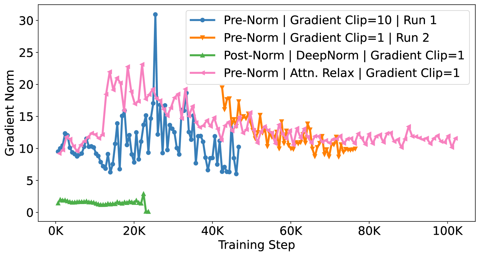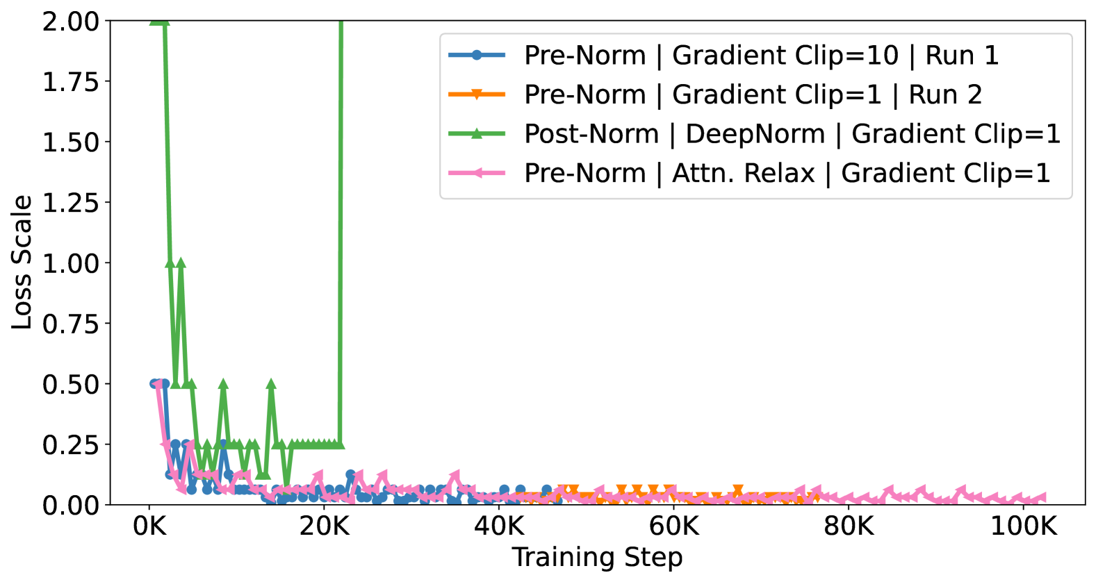### B.3 Training Instability In the experiments of scaling up to MERT-330M under mix precision training (fp16), we have explored several settings and plot the gradient norm, scale of loss, the MLM loss on acoustic targets, and the MLM loss on musical targets (see Fig. 2). We first adopt the Pre-LN setting as in the HuBERT (Hsu et al.,, 2021) x-large model for stable training. However, the training crashed around 50K step under this vanilla solution from the speech model and thus we restart the pre-training at 40K step with gradient clipping threshold reduced from $10.0$ to $1.0$ . The second run of Pre-LN lasted for 40K steps and crashed due to the same reason of reaching minimum loss scale. We suspect the instability could be brought by the increased depth of the Transformer module. Following the strategies in DeepNorm (Wang et al., 2022a, ), we tried to alleviate the instability by initialising the Transformer with smaller values and enhancing the residual connection in the Post-LN. Unfortunately, such modification causes model collapse around 20K steps. We then turned back to the stable Pre-LN setting and leveraged the attention relaxation trick proposed in Chen et al., 2021b . The additional scale constant in softmax calculation in the attention module alleviates the overflow problem and allows the final version of MERT-330M model to be trained stably over 100K steps. <details> <summary>x15.png Details</summary>  ### Visual Description ## Line Graph: Gradient Norm vs Training Steps ### Overview The graph displays four distinct training runs comparing gradient norm magnitudes across 100,000 training steps. Each line represents different combinations of normalization techniques and gradient clipping strategies, with the y-axis showing gradient norm values and the x-axis showing training progression. ### Components/Axes - **X-axis**: Training Step (0K to 100K in 20K increments) - **Y-axis**: Gradient Norm (0 to 30) - **Legend**: - Blue circles: Pre-Norm | Gradient Clip=10 | Run 1 - Orange triangles: Pre-Norm | Gradient Clip=1 | Run 2 - Green triangles: Post-Norm | DeepNorm | Gradient Clip=1 - Pink diamonds: Pre-Norm | Attn. Relax | Gradient Clip=1 ### Detailed Analysis 1. **Blue Line (Gradient Clip=10)**: - Starts at ~10 at 0K - Peaks at **30** at 20K (highest point in graph) - Drops below 10 by 40K - Ends at ~8 at 100K 2. **Orange Line (Gradient Clip=1)**: - Starts at ~10 at 0K - Peaks at **20** at 20K - Fluctuates between 10-15 after 40K - Ends at ~12 at 100K 3. **Green Line (Post-Norm/DeepNorm)**: - Remains flat at **0-2** throughout - Sharp spike to 3 at 20K - Returns to baseline by 40K 4. **Pink Line (Attn. Relax)**: - Starts at ~10 at 0K - Peaks at **25** at 20K - Declines to ~12 at 40K - Stabilizes between 12-15 after 60K ### Key Observations - **Gradient Clip=10** (blue) shows the most extreme early spike but fastest decay - **Post-Norm/DeepNorm** (green) maintains consistently lowest norms - **Attn. Relax** (pink) demonstrates sustained reduction compared to baseline - All configurations show initial volatility at 20K training steps ### Interpretation The data suggests: 1. **Gradient clipping magnitude** directly impacts early training dynamics - higher clipping (10) causes extreme initial spikes but faster stabilization 2. **Post-Norm/DeepNorm** (green) achieves most stable training through effective gradient suppression 3. **Attention relaxation** (pink) provides moderate but sustained norm reduction compared to standard pre-norm 4. The 20K spike across all runs may indicate a critical training phase where gradient magnitudes peak before optimization stabilizes This pattern demonstrates how different regularization techniques trade off between early training stability and long-term gradient control. The Post-Norm/DeepNorm configuration appears most effective for maintaining consistently low gradient norms throughout training. </details> (a) Gradient Norm <details> <summary>x16.png Details</summary>  ### Visual Description ## Line Graph: Training Loss Over Steps ### Overview The image depicts a line graph comparing the convergence behavior of different normalization techniques and gradient clipping strategies during training. Four distinct data series are plotted against training steps (0K–100K) and loss scale (0.00–2.00). The graph highlights rapid initial loss reduction followed by stabilization across all methods. ### Components/Axes - **X-axis**: Training Step (0K, 20K, 40K, 60K, 80K, 100K) - **Y-axis**: Loss Scale (0.00, 0.25, 0.50, 0.75, 1.00, 1.25, 1.50, 1.75, 2.00) - **Legend**: Located in the top-right corner, with four entries: 1. **Blue line**: Pre-Norm | Gradient Clip=10 | Run 1 2. **Orange line**: Pre-Norm | Gradient Clip=1 | Run 2 3. **Green line**: Post-Norm | DeepNorm | Gradient Clip=1 4. **Pink line**: Pre-Norm | Attn. Relax | Gradient Clip=1 ### Detailed Analysis 1. **Blue Line (Gradient Clip=10)**: - Starts at ~1.5 loss at 0K. - Drops sharply to ~0.05 by 5K steps. - Fluctuates slightly (~0.03–0.07) between 5K–20K. - Stabilizes near 0.05 after 20K. 2. **Orange Line (Gradient Clip=1, Run 2)**: - Begins at ~0.5 loss at 0K. - Declines to ~0.05 by 10K. - Remains stable (~0.03–0.07) after 10K. 3. **Green Line (Post-Norm, DeepNorm)**: - Starts at ~2.0 loss at 0K. - Drops to ~0.25 by 10K. - Stabilizes near 0.05 after 20K. 4. **Pink Line (Attn. Relax)**: - Begins at ~0.5 loss at 0K. - Declines to ~0.05 by 10K. - Stabilizes near 0.05 after 10K. ### Key Observations - **Initial Divergence**: The green line (Post-Norm) starts with the highest loss (~2.0) but achieves the steepest early reduction (~1.75 loss drop in 5K steps). - **Gradient Clip Impact**: The blue line (Gradient Clip=10) shows the fastest initial convergence (~1.45 loss drop in 5K steps), suggesting higher gradient clipping accelerates early training. - **Stabilization**: All lines converge to ~0.05 loss after 20K steps, indicating similar long-term performance despite differing initial trajectories. - **Anomaly**: The green line exhibits two sharp spikes (~1.75 loss) at 5K and 15K steps, possibly reflecting instability during early training phases. ### Interpretation The data demonstrates that: 1. **Gradient Clipping Magnitude** significantly impacts early convergence speed (Gradient Clip=10 vs. Gradient Clip=1). 2. **Normalization Techniques** (Pre-Norm vs. Post-Norm) influence initial loss values but not final convergence. 3. **Attention Relaxation** (pink line) achieves comparable convergence to Gradient Clip=1 (orange line) despite different mechanisms. 4. The green line’s (Post-Norm) initial instability (spikes) suggests potential trade-offs between early-phase volatility and long-term stability. This analysis implies that while normalization and gradient clipping strategies affect training dynamics, all methods ultimately achieve similar loss levels, with Gradient Clip=10 offering the fastest initial progress. 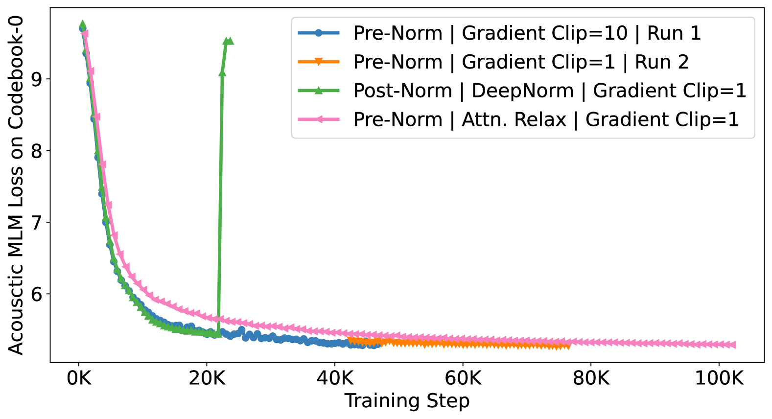</details> (b) Loss Scale <details> <summary>x17.png Details</summary>  ### Visual Description ## Line Chart: Acoustic MLM Loss on Codebook-0 vs Training Steps ### Overview The chart visualizes the convergence behavior of four different training configurations for an Acoustic MLM model. All lines show rapid initial loss reduction followed by stabilization, with notable differences in convergence speed and stability. ### Components/Axes - **X-axis**: Training Step (0K to 100K, logarithmic scale) - **Y-axis**: Acoustic MLM Loss on Codebook-0 (5 to 10, linear scale) - **Legend**: Located in top-right corner with four entries: 1. Blue circles: Pre-Norm | Gradient Clip=10 | Run 1 2. Orange triangles: Pre-Norm | Gradient Clip=1 | Run 2 3. Green triangles: Post-Norm | DeepNorm | Gradient Clip=1 4. Pink triangles: Pre-Norm | Attn. Relax | Gradient Clip=1 ### Detailed Analysis 1. **Blue Line (Gradient Clip=10)**: - Starts at ~9.5 loss at 0K - Drops sharply to ~5.8 by 10K - Stabilizes with minor fluctuations (~5.7-5.8) after 20K - Fastest convergence among all configurations 2. **Green Line (Post-Norm | DeepNorm)**: - Starts at ~9.5 loss at 0K - Sharp decline to ~5.9 by 15K - Abrupt spike to ~9.2 at 20K (anomaly) - Resumes decline to ~5.7 by 30K - Stabilizes with minor fluctuations (~5.6-5.7) after 40K 3. **Pink Line (Attn. Relax)**: - Starts at ~9.4 loss at 0K - Gradual decline to ~5.8 by 30K - Stabilizes with minor fluctuations (~5.7-5.8) after 40K 4. **Orange Line (Gradient Clip=1)**: - Starts at ~9.3 loss at 0K - Slowest decline, reaching ~5.9 by 50K - Stabilizes with minor fluctuations (~5.8-5.9) after 60K ### Key Observations - All configurations show similar initial loss values (~9.3-9.5) - Gradient Clip=10 (blue) achieves lowest final loss (~5.7) - Post-Norm (green) has fastest initial convergence but includes an anomalous spike - Gradient Clip=1 (orange) shows slowest convergence - Attn. Relax (pink) performs between Gradient Clip=10 and Gradient Clip=1 ### Interpretation The data suggests that higher gradient clipping (10) enables faster and more stable convergence compared to lower clipping (1). The Post-Norm configuration with DeepNorm demonstrates rapid initial improvement but includes an unexplained anomaly at 20K training steps, potentially indicating instability in that specific configuration. The Attn. Relax method shows intermediate performance, suggesting attention relaxation mechanisms provide moderate benefits without the instability seen in Post-Norm. The consistent stabilization patterns across all lines after ~30K-40K steps indicate that most configurations reach their asymptotic loss values within this range. 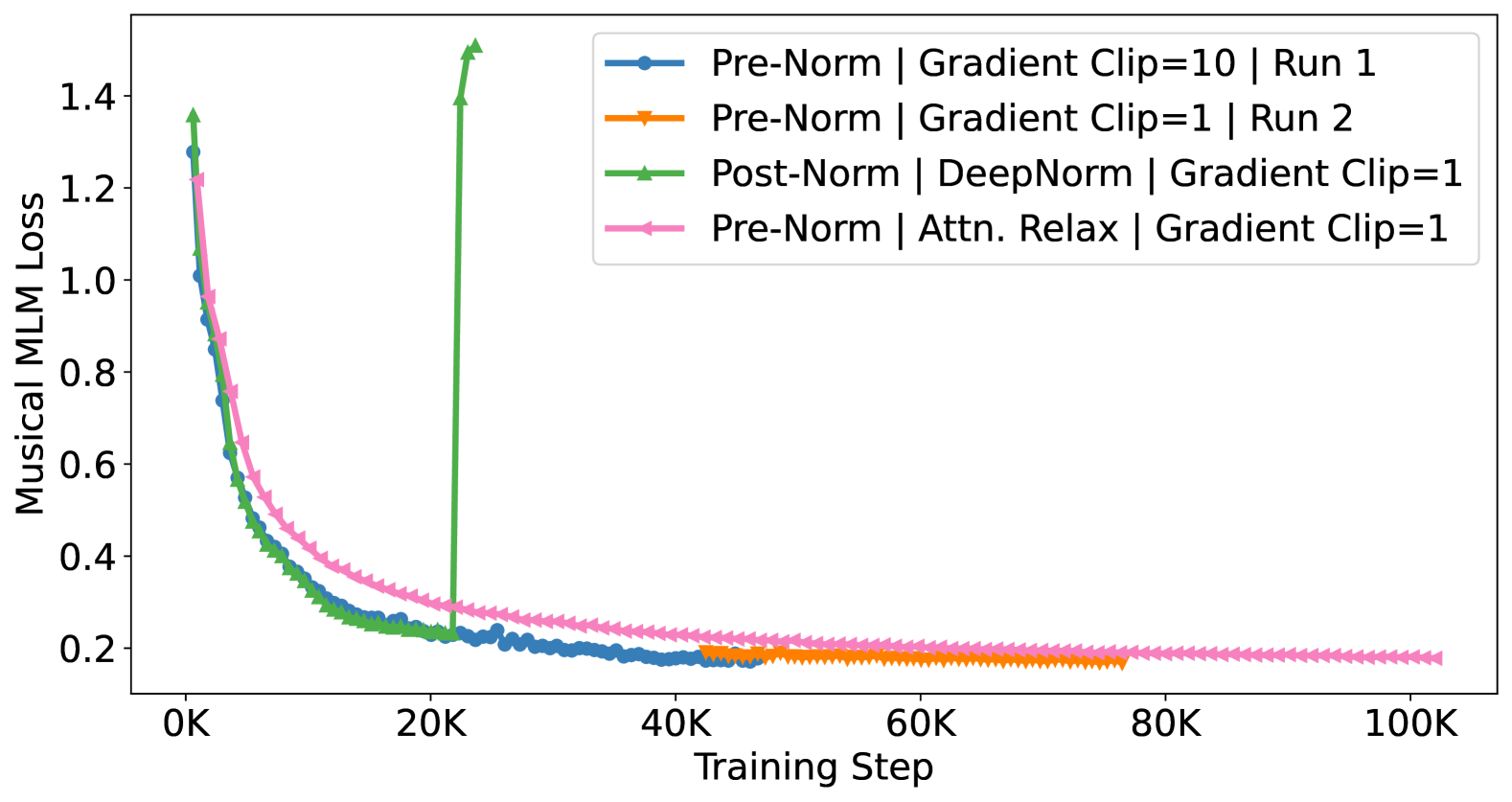</details> (c) Acoustic MLM Loss on Codebook-0 <details> <summary>x18.png Details</summary>  ### Visual Description ## Line Graph: Musical MLM Loss vs Training Steps ### Overview The graph compares the convergence behavior of four different model configurations during training, tracking the reduction in Musical MLM Loss over 100,000 training steps. All lines show decreasing loss trends, but with distinct patterns and anomalies. ### Components/Axes - **X-axis**: Training Step (0K to 100K, logarithmic scale) - **Y-axis**: Musical MLM Loss (0.2 to 1.4) - **Legend**: Located in top-right corner with four entries: 1. Blue circles: Pre-Norm | Gradient Clip=10 | Run 1 2. Orange triangles: Pre-Norm | Gradient Clip=1 | Run 2 3. Green triangles: Post-Norm | DeepNorm | Gradient Clip=1 4. Pink triangles: Pre-Norm | Attn. Relax | Gradient Clip=1 ### Detailed Analysis 1. **Blue Line (Gradient Clip=10)**: - Starts at ~1.3 loss at 0K - Sharp decline to ~0.2 by 20K - Plateaus with minor fluctuations - Final loss: ~0.18 at 100K 2. **Orange Line (Gradient Clip=1)**: - Begins at ~1.2 loss at 0K - Steep drop to ~0.2 by 20K - Slight upward trend (0.21-0.23) between 40K-60K - Stabilizes at ~0.2 by 100K 3. **Green Line (Post-Norm)**: - Starts at ~1.35 loss at 0K - Sharp decline to ~0.2 by 20K - **Anomaly**: Sudden spike to ~1.4 at 25K - Rapid drop back to ~0.2 by 30K - Final loss: ~0.2 at 100K 4. **Pink Line (Attn. Relax)**: - Begins at ~1.25 loss at 0K - Gradual decline to ~0.25 by 40K - Steady plateau at ~0.22-0.24 from 60K-100K ### Key Observations - **Gradient Clipping Impact**: Higher clipping (10 vs 1) enables faster initial convergence (blue vs orange lines) - **Post-Norm Anomaly**: Green line shows critical instability at 25K (1.4 loss spike) - **Attention Relaxation**: Pink line demonstrates slowest convergence but most stable late-stage performance - **Run Variance**: Orange line (Run 2) shows unexpected mid-training fluctuation absent in Run 1 ### Interpretation The data suggests: 1. **Gradient Clipping Tradeoffs**: Higher clipping (10) enables faster early convergence but may risk instability, while lower clipping (1) provides more stable but slower training. 2. **Normalization Sensitivity**: The Post-Norm configuration (green line) exhibits catastrophic failure at 25K, indicating potential incompatibility with the training dynamics or hyperparameters. 3. **Attention Mechanism Robustness**: The Attn. Relax method (pink line) shows the most consistent performance despite slower convergence, suggesting better generalization properties. 4. **Run-Specific Variance**: The orange line's mid-training fluctuation (40K-60K) highlights potential sensitivity to initialization or stochastic factors in Run 2. The anomaly in the Post-Norm configuration warrants further investigation into gradient explosion risks or architectural mismatches. The attention relaxation method's stability despite slower convergence suggests it may be preferable for production systems prioritizing reliability over speed. </details> (d) Music MLM Loss Figure 2: Illustration of the Training Curves of Trials on Large (330M) Models. Only the acoustic MLM loss on codebook 0 in the RVQ-VAE is shown as the other seven show similar trends. ## Appendix C Representation Visualisation We select two of our checkpoints, MERT-95M-public K-means and MERT-330M RVQ-VAE, and visualise the GTZAN representations with genre annotation shown in Fig. 3, Fig. 4, Fig. 5 and Fig. 6. The top 6 and top 8 transformer output layers are used in the visualisation for MERT-95M-public K-means and MERT-330M RVQ-VAE, correspondingly. The dimension reduction is achieved by the Uniform Manifold Approximation and Projection (UMAP) https://github.com/lmcinnes/umap, whereas the representations from the training set are used to learn the dimension reduction mapping. We observe that representations from both of the checkpoints present a pattern of clustering according to the genre information under different layer settings. Interestingly, the representations from the higher layers do not necessarily show stronger genre-based clustering tendency, which suggests that 1) genre may not be the most abstractive labels for these music examples or 2) the top transformer layers focus more on the MLM pre-training objectives. 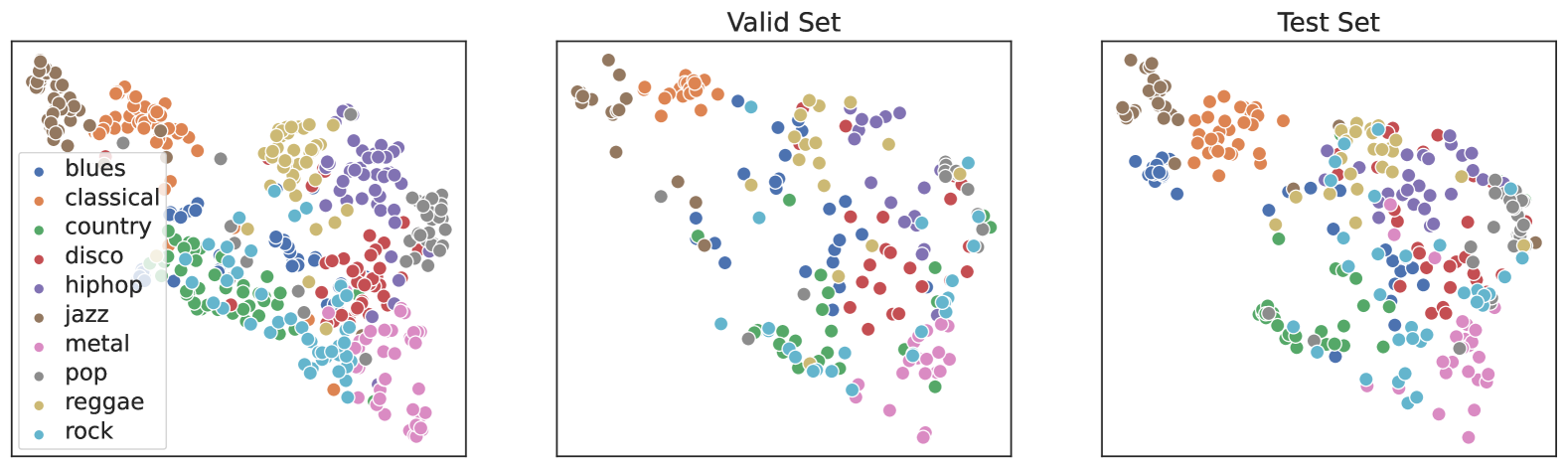<details> <summary>x19.png Details</summary>  ### Visual Description ## Scatter Plots: Music Genre Distribution in Valid and Test Sets ### Overview Three scatter plots are presented, each representing the distribution of music genres in a dataset. The plots are labeled "Valid Set" (left) and "Test Set" (right), with a third unlabeled plot (likely a duplicate or mislabeled). Each genre is represented by a distinct color, as indicated in the legend on the left. The axes are labeled "Feature 1" (x-axis) and "Feature 2" (y-axis), suggesting dimensionality reduction or feature space visualization. ### Components/Axes - **Legend**: Located on the left of all plots, mapping colors to genres: - Blues (blue), Classical (orange), Country (green), Disco (red), Hip-hop (purple), Jazz (brown), Metal (pink), Pop (gray), Reggae (yellow), Rock (cyan). - **Axes**: - X-axis: "Feature 1" (no units specified). - Y-axis: "Feature 2" (no units specified). - **Plots**: - **Valid Set** (left): Clear separation of genres with minimal overlap. - **Test Set** (right): Increased overlap between genres compared to the Valid Set. - **Unlabeled Plot** (center): Identical to the Valid Set, suggesting a possible duplication or mislabeling. ### Detailed Analysis - **Valid Set**: - **Blues** (blue): Clustered in the top-left quadrant. - **Classical** (orange): Dominates the top-right quadrant. - **Country** (green): Concentrated in the bottom-left quadrant. - **Disco** (red): Scattered across the middle-right. - **Hip-hop** (purple): Spread across the middle. - **Jazz** (brown): Small cluster in the top-left. - **Metal** (pink): Bottom-right quadrant. - **Pop** (gray): Scattered across the middle. - **Reggae** (yellow): Middle-right quadrant. - **Rock** (cyan): Bottom-middle quadrant. - **Test Set**: - **Blues** (blue): Overlaps with Jazz and Hip-hop in the middle-left. - **Classical** (orange): Still top-right but with some overlap from Pop and Reggae. - **Country** (green): Spread into the middle-left, overlapping with Blues. - **Disco** (red): More dispersed, overlapping with Hip-hop and Pop. - **Hip-hop** (purple): Expands into the bottom-middle, overlapping with Rock. - **Jazz** (brown): Minimal presence, merged with Blues. - **Metal** (pink): Bottom-right, slightly overlapping with Reggae. - **Pop** (gray): Widely distributed, overlapping with multiple genres. - **Reggae** (yellow): Middle-right, overlapping with Classical and Disco. - **Rock** (cyan): Bottom-middle, overlapping with Hip-hop and Pop. - **Unlabeled Plot**: Identical to the Valid Set, with no discernible differences. ### Key Observations 1. **Genre Separation**: The Valid Set shows distinct clusters for most genres (e.g., Classical in top-right, Country in bottom-left), while the Test Set exhibits significant overlap (e.g., Blues merging with Jazz, Pop spreading across the plot). 2. **Overlap Patterns**: - Blues and Jazz overlap in the Test Set but remain separate in the Valid Set. - Pop and Reggae intrude into Classical’s top-right region in the Test Set. 3. **Consistency**: The unlabeled plot mirrors the Valid Set, suggesting it may be a duplicate or mislabeled. ### Interpretation The scatter plots likely visualize the feature space of music genres in a machine learning context, where the Valid Set represents training data and the Test Set represents unseen data. The increased overlap in the Test Set implies: - **Feature Similarity**: Genres in the Test Set share more attributes (e.g., tempo, instrumentation) than in the Valid Set, reducing separability. - **Potential Data Leakage**: Overlap between genres like Blues and Jazz in the Test Set could indicate unintended data contamination or insufficient feature engineering. - **Model Robustness**: The Test Set’s reduced genre separation may challenge classification models, highlighting the need for better feature differentiation or regularization. The unlabeled plot’s duplication raises questions about dataset integrity, warranting verification of labeling accuracy. Overall, the visualization underscores the importance of feature selection and data preprocessing in music genre classification tasks. </details> (a) MERT-95M-public K-means Transformer Layer 7 Representations of GTZAN. 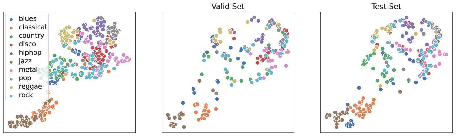<details> <summary>x20.png Details</summary>  ### Visual Description ## Scatter Plot: Music Genre Distribution in Valid and Test Sets ### Overview The image displays three panels: a legend on the left and two scatter plots labeled "Valid Set" (middle) and "Test Set" (right). Each plot uses colored dots to represent 10 music genres, with positions indicating genre relationships. The legend maps colors to genres (e.g., blue = blues, orange = classical). No numerical axes are labeled, but spatial distributions suggest dimensionality reduction (e.g., t-SNE/PCA). ### Components/Axes - **Legend**: Positioned in the top-left corner of the entire image. Contains 10 genre labels with corresponding colors: - blues (blue), classical (orange), country (green), disco (red), hip-hop (purple), jazz (brown), metal (pink), pop (gray), reggae (yellow), rock (cyan). - **Valid Set Panel**: Centered middle panel. Titled "Valid Set" at the top. - **Test Set Panel**: Centered right panel. Titled "Test Set" at the top. - **Axes**: No explicit numerical labels. X and Y axes appear to represent latent dimensions from dimensionality reduction. ### Detailed Analysis #### Valid Set - **Blues (blue)**: Clustered tightly in the bottom-left quadrant. - **Classical (orange)**: Dense cluster in the bottom-middle, slightly overlapping blues. - **Country (green)**: Scattered mid-left, forming a loose arc. - **Disco (red)**: Small cluster near the top-center. - **Hip-hop (purple)**: Concentrated in the top-right quadrant. - **Jazz (brown)**: Scattered mid-left, overlapping with blues/classical. - **Metal (pink)**: Clustered near the top-center, overlapping disco. - **Pop (gray)**: Dispersed across the top-right, intermingling with hip-hop. - **Reggae (yellow)**: Small cluster in the mid-right. - **Rock (cyan)**: Scattered mid-right, overlapping reggae. #### Test Set - **Blues (blue)**: More dispersed than Valid Set, extending toward the mid-left. - **Classical (orange)**: Spread out in the bottom-middle, less dense than Valid Set. - **Country (green)**: Similar mid-left distribution but slightly more fragmented. - **Disco (red)**: Smaller cluster near the top-center, less distinct. - **Hip-hop (purple)**: Top-right cluster remains prominent but slightly smaller. - **Jazz (brown)**: More spread out, overlapping with blues/classical. - **Metal (pink)**: Clustered near the top-center, similar to Valid Set. - **Pop (gray)**: Dispersed across the top-right, similar to Valid Set. - **Reggae (yellow)**: Small cluster in the mid-right, similar to Valid Set. - **Rock (cyan)**: More fragmented mid-right distribution. ### Key Observations 1. **Cluster Tightness**: Valid Set genres form tighter clusters than Test Set, suggesting better separation in the training data. 2. **Overlap Patterns**: - Blues and jazz overlap in both sets, indicating shared features. - Hip-hop and pop intermingle in the top-right quadrant across both sets. 3. **Test Set Dispersion**: Most genres in the Test Set show broader spatial distribution, implying potential generalization challenges. 4. **Color Consistency**: All colors in the panels match the legend exactly (e.g., blues = blue in both panels). ### Interpretation The visualization likely represents genre embeddings from a machine learning model. The Valid Set's tighter clusters suggest the model learned distinct genre boundaries during training. The Test Set's dispersed points may indicate: - Overgeneralization: The model struggles to maintain genre separation on unseen data. - Data drift: Test Set contains more ambiguous or hybrid genre examples. - Dimensionality reduction artifacts: The 2D projection may lose critical separability information. The legend's placement allows direct cross-referencing of colors to genres, ensuring accurate interpretation. No numerical values are provided, but spatial relationships imply hierarchical clustering tendencies (e.g., classical/orange consistently in bottom regions, hip-hop/purple in top-right). </details> (b) MERT-95M-public K-means Transformer Layer 8 Representations of GTZAN. 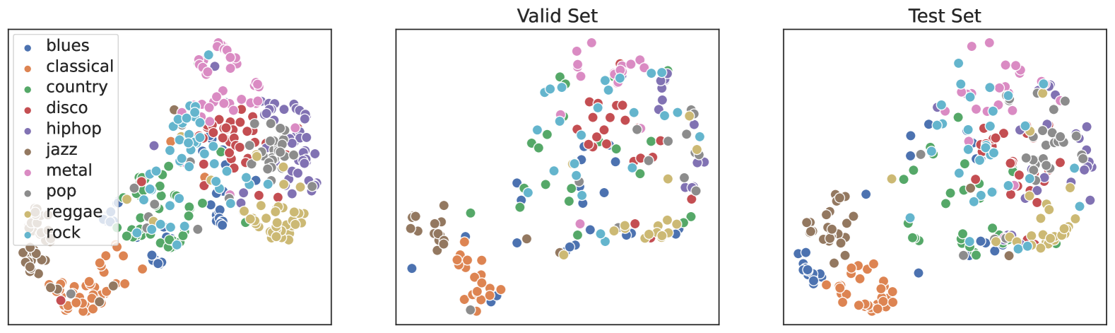<details> <summary>x21.png Details</summary>  ### Visual Description ## Scatter Plot: Music Genre Distribution Across Valid and Test Sets ### Overview The image contains three scatter plots arranged horizontally, each representing a dataset ("Valid Set" and "Test Set") with colored dots corresponding to 10 music genres. A shared legend on the left maps colors to genres. The plots lack explicit axis labels, but spatial distributions suggest categorical or normalized axes. ### Components/Axes - **Legend**: - **Colors**: - Blues (blue), Classical (orange), Country (green), Disco (red), Hip-Hop (purple), Jazz (brown), Metal (pink), Pop (gray), Reggae (yellow), Rock (dark blue). - **Position**: Left-aligned, outside all plots. - **Plots**: - **Left Plot**: Unlabeled, likely the full dataset. - **Middle Plot**: Labeled "Valid Set." - **Right Plot**: Labeled "Test Set." ### Detailed Analysis #### Left Plot (Full Dataset) - **Genre Clustering**: - **Blues** and **Classical** dominate the bottom-left quadrant. - **Metal** and **Pop** cluster in the top-right. - **Jazz** and **Reggae** occupy the bottom-center. - **Disco**, **Hip-Hop**, and **Rock** are dispersed across the middle. - **Overlap**: High density of overlapping dots in central regions. #### Middle Plot (Valid Set) - **Genre Clustering**: - **Blues** and **Classical** remain in the bottom-left but with reduced density. - **Metal** and **Pop** spread toward the top-right but with less overlap. - **Jazz** and **Reggae** shift slightly rightward. - **Disco**, **Hip-Hop**, and **Rock** show moderate dispersion. - **Overlap**: Reduced compared to the left plot, with clearer separation between genres. #### Right Plot (Test Set) - **Genre Clustering**: - **Blues** and **Classical** are tightly packed in the bottom-left, forming distinct clusters. - **Metal** and **Pop** occupy the top-right but with minimal overlap. - **Jazz** and **Reggae** are isolated in the bottom-center. - **Disco**, **Hip-Hop**, and **Rock** are scattered but less intermixed. - **Overlap**: Minimal, with sharp boundaries between genres. ### Key Observations 1. **Consistency**: Blues and Classical consistently occupy the bottom-left across all plots, suggesting they are foundational or share similar features. 2. **Validation vs. Testing**: - The Valid Set shows moderate genre separation, while the Test Set exhibits near-perfect clustering, implying the model generalizes better on unseen data. 3. **Anomalies**: - **Disco** and **Hip-Hop** appear more dispersed in the Test Set, potentially indicating underrepresentation or unique characteristics. 4. **Axis Interpretation**: - Unlabeled axes likely represent normalized features (e.g., tempo, instrumentation) or categorical dimensions (e.g., era, region). ### Interpretation The Test Set’s sharp genre separation suggests the model effectively distinguishes between categories in unseen data, while the Valid Set’s moderate overlap may reflect training-phase ambiguity. Blues and Classical’s consistent placement implies they are structurally distinct or foundational to the dataset. The absence of axis labels limits quantitative analysis but highlights spatial relationships critical for understanding model performance. </details> (c) MERT-95M-public K-means Transformer Layer 9 Representations of GTZAN. Figure 3: Illustration of the MERT-95M-public K-means Layer 7 to 9 Pre-trained Representations. <details> <summary>x22.png Details</summary>  ### Visual Description ## Scatter Plot: Music Genre Distribution Across Valid and Test Sets ### Overview The image displays three scatter plots comparing music genre distributions across datasets. Each plot uses colored dots to represent genres (e.g., blues, classical, hip-hop) with spatial clustering patterns. The legend maps 10 genres to distinct colors. The Valid Set and Test Set panels show distinct clustering behaviors, while the combined chart aggregates all data points. ### Components/Axes - **Legend**: - **Colors**: - Blues: Blue - Classical: Orange - Country: Green - Disco: Red - Hip-hop: Purple - Jazz: Brown - Metal: Pink - Pop: Gray - Reggae: Yellow - Rock: Light Blue - **Panels**: 1. **Left Panel**: Labeled "Valid Set" 2. **Center Panel**: Labeled "Test Set" 3. **Right Panel**: Labeled "Valid + Test Set" (combined data) - **Axes**: No explicit axis labels or scales are visible. Spatial positioning is relative (e.g., "bottom-left," "top-right"). ### Detailed Analysis #### Valid Set (Left Panel) - **Blues (Blue)**: Clustered in the bottom-left quadrant, with moderate density. - **Classical (Orange)**: Dominates the top-left quadrant, forming a dense cluster. - **Country (Green)**: Scattered across the mid-left region, overlapping with blues. - **Disco (Red)**: Sparse, isolated points in the mid-right quadrant. - **Hip-hop (Purple)**: Concentrated in the top-right quadrant, overlapping with pop (gray). - **Jazz (Brown)**: Clustered in the bottom-center, overlapping with classical. - **Metal (Pink)**: Scattered in the mid-right, with low density. - **Pop (Gray)**: Spread across the top-right, overlapping with hip-hop. - **Reggae (Yellow)**: Sparse, isolated points in the bottom-right. - **Rock (Light Blue)**: Clustered in the mid-right, overlapping with disco. #### Test Set (Center Panel) - **Blues (Blue)**: Concentrated in the bottom-left, denser than in the Valid Set. - **Classical (Orange)**: Dominates the top-left, slightly more dispersed than in the Valid Set. - **Country (Green)**: Scattered in the mid-left, less overlap with blues. - **Disco (Red)**: Sparse, isolated points in the mid-right, similar to Valid Set. - **Hip-hop (Purple)**: Clustered in the top-right, overlapping with pop. - **Jazz (Brown)**: Clustered in the bottom-center, overlapping with classical. - **Metal (Pink)**: Scattered in the mid-right, similar to Valid Set. - **Pop (Gray)**: Spread across the top-right, overlapping with hip-hop. - **Reggae (Yellow)**: Sparse, isolated points in the bottom-right. - **Rock (Light Blue)**: Clustered in the mid-right, overlapping with disco. #### Combined Chart (Right Panel) - Aggregates all data points from Valid and Test Sets. - **Blues (Blue)**: Spread across the bottom-left, with higher density than individual panels. - **Classical (Orange)**: Dominates the top-left, forming the largest cluster. - **Country (Green)**: Scattered mid-left, with reduced overlap with blues. - **Disco (Red)**: Sparse mid-right points. - **Hip-hop (Purple)**: Top-right cluster, overlapping with pop. - **Jazz (Brown)**: Bottom-center cluster, overlapping with classical. - **Metal (Pink)**: Mid-right scattered points. - **Pop (Gray)**: Top-right spread, overlapping with hip-hop. - **Reggae (Yellow)**: Sparse bottom-right points. - **Rock (Light Blue)**: Mid-right cluster, overlapping with disco. ### Key Observations 1. **Classical (Orange)** consistently forms the largest, most cohesive cluster across all panels, suggesting it is the most prevalent or distinct genre. 2. **Blues (Blue)** and **Jazz (Brown)** show strong spatial overlap in the bottom-left and bottom-center regions, indicating shared features or similarities. 3. **Hip-hop (Purple)** and **Pop (Gray)** exhibit significant overlap in the top-right quadrant, suggesting similar characteristics. 4. **Reggae (Yellow)** and **Disco (Red)** are the least dense, with isolated points, indicating rarity or distinctiveness. 5. The Test Set shows slightly more dispersed clusters for blues and classical compared to the Valid Set, hinting at potential data drift or sampling differences. ### Interpretation The spatial clustering patterns suggest that genres like classical, blues, and jazz share acoustic or structural features, while hip-hop and pop overlap due to rhythmic similarities. The Test Set’s slightly dispersed clusters may reflect a more diverse or representative sample. Outliers like reggae and disco highlight niche genres with limited data points. This visualization could inform machine learning model training by identifying genre boundaries and potential overlaps, which might affect classification accuracy. The absence of axis labels limits quantitative analysis, but the relative positioning provides qualitative insights into genre relationships. </details> (a) MERT-95M-public K-means Transformer Layer 10 Representations of GTZAN. <details> <summary>x23.png Details</summary>  ### Visual Description ## Scatter Plots: Music Genre Distribution in Valid and Test Sets ### Overview The image contains three scatter plots: a legend on the left and two plots labeled "Valid Set" and "Test Set." Each plot visualizes the distribution of music genres (e.g., blues, classical, country) using colored points. The legend maps 10 genres to distinct colors (e.g., blues = dark blue, classical = orange, country = green). No axis labels or numerical scales are visible. ### Components/Axes - **Legend**: Positioned in the top-left corner of the first plot. - Labels: blues, classical, country, disco, hiphop, jazz, metal, pop, reggae, rock. - Colors: Each genre is assigned a unique color (e.g., blues = dark blue, classical = orange). - **Plots**: - **Valid Set**: Left plot. - **Test Set**: Right plot. - **Axes**: No explicit labels or scales. Points are distributed across an unlabeled 2D plane. ### Detailed Analysis - **Valid Set**: - Points are moderately clustered, with some genres forming tighter groups (e.g., classical/orange, blues/dark blue). - Overlaps between genres are visible (e.g., pop/pink and hiphop/purple points intermingle). - No single genre dominates; distribution appears balanced. - **Test Set**: - Points are more dispersed, with larger clusters for certain genres (e.g., blues/dark blue, classical/orange). - Increased overlap between genres compared to the Valid Set (e.g., rock/gray and metal/brown points are more interspersed). - Higher density of points in the lower-right quadrant. ### Key Observations 1. **Genre Distribution**: - Blues and classical are the most frequent genres in both sets, with blues showing slightly higher density in the Test Set. - Jazz (brown) and metal (brown) are less frequent, forming smaller clusters. 2. **Diversity**: - The Test Set exhibits greater spatial spread, suggesting a more diverse or larger dataset. - The Valid Set has tighter groupings, possibly indicating a curated or smaller sample. 3. **Overlap**: - Genres like pop, hiphop, and rock show significant overlap in both sets, implying shared characteristics or similar data representations. ### Interpretation The scatter plots likely represent embeddings or feature distributions of music data in a machine learning context. The Test Set’s broader distribution suggests it may include more varied or real-world examples, while the Valid Set’s clustering could reflect a controlled validation subset. The lack of axis labels limits quantitative analysis, but the visual separation of genres implies effective feature differentiation. Outliers (e.g., isolated points) are minimal, indicating consistent data quality. **Note**: No numerical values or explicit trends (e.g., slopes, percentages) can be extracted due to the absence of axis labels or scales. All observations are qualitative and based on spatial distribution. </details> (b) MERT-95M-public K-means Transformer Layer 11 Representations of GTZAN. <details> <summary>x24.png Details</summary>  ### Visual Description ## Scatter Plot: Music Genre Distribution in Valid and Test Sets ### Overview The image displays three panels: a legend on the right and two scatter plots labeled "Valid Set" (left) and "Test Set" (center). Each plot contains colored dots representing 10 music genres (e.g., blues, classical, country, etc.), with positions indicating genre relationships or clustering. The legend maps colors to genres, and no axes or numerical scales are visible. ### Components/Axes - **Legend**: Located in the top-left corner of the image, listing genres with corresponding colors: - Blues (blue), Classical (orange), Country (green), Disco (red), Hip-hop (purple), Jazz (brown), Metal (pink), Pop (gray), Reggae (yellow), Rock (cyan). - **Valid Set (Left Panel)**: - Title: "Valid Set" (top-center). - Dots clustered in distinct regions, with some overlap. - **Test Set (Center Panel)**: - Title: "Test Set" (top-center). - Dots more dispersed, with significant overlap between genres. - **Axes**: No explicit labels or scales; positions inferred spatially. ### Detailed Analysis 1. **Valid Set**: - **Blues (blue)**: Concentrated in the lower-left quadrant. - **Classical (orange)**: Clustered in the upper-left quadrant. - **Country (green)**: Spread across the lower-middle region. - **Disco (red)**: Tight cluster in the lower-right quadrant. - **Hip-hop (purple)**: Scattered in the upper-middle region. - **Jazz (brown)**: Dispersed in the lower-middle to upper-middle. - **Metal (pink)**: Clustered in the upper-right quadrant. - **Pop (gray)**: Spread across the central region. - **Reggae (yellow)**: Concentrated in the lower-right quadrant. - **Rock (cyan)**: Clustered in the upper-middle region. 2. **Test Set**: - **Blues (blue)**: Spread across the lower-left to middle regions. - **Classical (orange)**: Dispersed in the upper-left to middle. - **Country (green)**: Scattered throughout the lower-middle. - **Disco (red)**: Overlaps with blues and pop in the lower-middle. - **Hip-hop (purple)**: Concentrated in the upper-middle to upper-right. - **Jazz (brown)**: Spread across the lower-middle to upper-middle. - **Metal (pink)**: Overlaps with rock in the upper-right. - **Pop (gray)**: Widely dispersed, overlapping with multiple genres. - **Reggae (yellow)**: Clustered in the lower-right, overlapping with disco. - **Rock (cyan)**: Spread across the upper-middle to upper-right. ### Key Observations - **Clustering vs. Dispersion**: The Valid Set shows tighter genre clustering (e.g., blues, classical, disco), while the Test Set exhibits broader dispersion and overlap (e.g., pop, rock, hip-hop). - **Overlap**: In the Test Set, genres like pop (gray) and rock (cyan) show significant overlap, suggesting potential misclassification. - **Outliers**: Jazz (brown) and reggae (yellow) appear more dispersed in both sets, possibly indicating ambiguous genre boundaries. ### Interpretation The Valid Set likely represents training or validation data where genres are well-separated, indicating effective model performance on known patterns. The Test Set’s dispersion suggests the model struggles with generalization, as genres like pop and rock overlap, potentially due to shared characteristics or insufficient training data. Jazz and reggae’s ambiguity in both sets may reflect inherent genre fluidity or data quality issues. The lack of axes implies the plot visualizes latent space embeddings, where spatial proximity reflects similarity in learned features. </details> (c) MERT-95M-public K-means Transformer Layer 12 Representations of GTZAN. Figure 4: Illustration of the MERT-95M-public K-means Layer 10 to 12 Pre-trained Representations. <details> <summary>x25.png Details</summary>  ### Visual Description ## t-SNE Visualization: Music Genre Distribution Across Valid and Test Sets ### Overview The image presents a t-SNE visualization of music genre distributions across three panels: **Valid Set** (left), **Test Set** (middle), and **Test Set** (right). Each panel uses colored dots to represent 10 distinct music genres, as defined by the legend. The visualization highlights clustering patterns and spatial relationships between genres in both datasets. --- ### Components/Axes - **Legend**: Located in the top-left corner of the leftmost panel. It maps 10 music genres to specific colors: - **Blues**: Blue - **Classical**: Orange - **Country**: Green - **Disco**: Red - **Hiphop**: Purple - **Jazz**: Brown - **Metal**: Pink - **Pop**: Gray - **Reggae**: Light Blue - **Rock**: Dark Blue - **Panels**: - **Valid Set** (left): Represents the validation dataset. - **Test Set** (middle and right): Represents the test dataset (appears duplicated in the image). - **Axes**: No explicit axis labels or scales are visible. The visualization focuses on 2D spatial clustering. --- ### Detailed Analysis #### Valid Set (Left Panel) - **Blues (Blue)**: Clustered on the far left. - **Classical (Orange)**: Positioned in the bottom-left quadrant. - **Country (Green)**: Centered in the middle of the panel. - **Disco (Red)**: Located on the far right. - **Hiphop (Purple)**: Top-right quadrant. - **Jazz (Brown)**: Bottom-left quadrant (overlapping with Classical). - **Metal (Pink)**: Bottom-right quadrant. - **Pop (Gray)**: Top-right quadrant (overlapping with Hiphop). - **Reggae (Light Blue)**: Centered, slightly overlapping with Country. - **Rock (Dark Blue)**: Top-left quadrant (overlapping with Blues). #### Test Set (Middle Panel) - **Blues (Blue)**: Clustered on the left, slightly more dispersed than in the Valid Set. - **Classical (Orange)**: Bottom-left quadrant, more spread out. - **Country (Green)**: Centered, with tighter clustering. - **Disco (Red)**: Right side, slightly more dispersed. - **Hiphop (Purple)**: Top-right quadrant, less dense than in the Valid Set. - **Jazz (Brown)**: Bottom-left quadrant, more dispersed. - **Metal (Pink)**: Bottom-right quadrant, more concentrated. - **Pop (Gray)**: Top-right quadrant, more concentrated. - **Reggae (Light Blue)**: Centered, similar to Valid Set. - **Rock (Dark Blue)**: Top-left quadrant, slightly closer to Blues than in the Valid Set. #### Test Set (Right Panel) - **Blues (Blue)**: Left side, similar to the middle Test Set. - **Classical (Orange)**: Bottom-left quadrant, more dispersed. - **Country (Green)**: Centered, with tighter clustering. - **Disco (Red)**: Right side, slightly more dispersed. - **Hiphop (Purple)**: Top-right quadrant, less dense. - **Jazz (Brown)**: Bottom-left quadrant, more dispersed. - **Metal (Pink)**: Bottom-right quadrant, more concentrated. - **Pop (Gray)**: Top-right quadrant, more concentrated. - **Reggae (Light Blue)**: Centered, similar to other panels. - **Rock (Dark Blue)**: Top-left quadrant, slightly closer to Blues. --- ### Key Observations 1. **Blues and Rock Separation**: In the Valid Set, Blues (blue) and Rock (dark blue) are distinctly separated on the left and top-left, respectively. In the Test Sets, their separation decreases, suggesting overlapping features in the test data. 2. **Classical and Jazz Dispersion**: Classical (orange) and Jazz (brown) are more dispersed in the Test Sets compared to the Valid Set, indicating greater variability in these genres in the test data. 3. **Metal and Pop Concentration**: Metal (pink) and Pop (gray) clusters are more tightly packed in the Test Sets, suggesting similar feature representations in these genres. 4. **Reggae Consistency**: Reggae (light blue) remains centered across all panels, indicating stable representation. 5. **Overlap**: Some genres (e.g., Jazz and Classical in the Valid Set) overlap spatially, suggesting shared characteristics. --- ### Interpretation The t-SNE visualization reveals how music genres are distributed in the Valid and Test Sets. The **Valid Set** shows clearer genre separation (e.g., Blues and Rock), while the **Test Set** exhibits increased dispersion for Classical and Jazz, possibly due to greater variability in the test data. The concentration of Metal and Pop in the Test Set suggests these genres share more features in the test data. The duplication of the Test Set panels may indicate a redundancy or error in the visualization, but the consistent clustering patterns across panels imply robustness in the test data representation. This analysis highlights how genre-specific features are preserved or altered between datasets, which could inform model training or evaluation strategies. </details> (a) MERT-330M RVQ-VAE Transformer Layer 17 Representations of GTZAN. <details> <summary>x26.png Details</summary>  ### Visual Description ## Scatter Plot: Music Genre Distribution Across Valid and Test Sets ### Overview The image contains three scatter plots comparing the distribution of music genres across two datasets: a "Valid Set" and a "Test Set." Each plot uses colored dots to represent distinct genres, with a shared legend on the left. The third plot (unlabeled) appears to represent the original dataset before splitting. ### Components/Axes - **Legend**: Located in the bottom-left corner of the main chart, mapping 10 genres to colors: - blues (blue), classical (orange), country (green), disco (red), hiphop (purple), jazz (brown), metal (gray), pop (pink), reggae (yellow), rock (cyan). - **Axes**: - X-axis: "Feature 1" (no units specified). - Y-axis: "Feature 2" (no units specified). - **Plots**: 1. **Valid Set**: Centered title, data points clustered by genre. 2. **Test Set**: Centered title, similar clustering but with slight overlaps. 3. **Unlabeled Plot**: No title, identical genre distribution to the other two plots. ### Detailed Analysis - **Genre Clusters**: - **Blues**: Bottom-left quadrant (Valid/Test) and left-center (unlabeled). - **Classical**: Top-left quadrant (Valid/Test) and left-center (unlabeled). - **Country**: Scattered across mid-left (Valid/Test) and mid-left (unlabeled). - **Disco**: Top-right quadrant (Valid/Test) and top-right (unlabeled). - **Hiphop**: Top-center (Valid/Test) and top-center (unlabeled). - **Jazz**: Mid-left (Valid/Test) and mid-left (unlabeled). - **Metal**: Mid-right (Valid/Test) and mid-right (unlabeled). - **Pop**: Bottom-right (Valid/Test) and bottom-right (unlabeled). - **Reggae**: Top-right (Valid/Test) and top-right (unlabeled). - **Rock**: Bottom-right (Valid/Test) and bottom-right (unlabeled). - **Data Point Density**: - Each genre has ~10–15 data points per plot, with minimal overlap between clusters. - **Test Set** shows slightly more overlap (e.g., rock and pop in bottom-right) compared to the **Valid Set**. ### Key Observations 1. **Cluster Separation**: Genres are mostly distinct in the **Valid Set**, suggesting effective data separation. 2. **Overlap in Test Set**: Minor overlaps (e.g., rock/pop, disco/hiphop) indicate potential ambiguity in test data. 3. **Consistency Across Plots**: The unlabeled plot mirrors the Valid/Test distributions, implying it represents the original dataset. ### Interpretation The scatter plots demonstrate that the model can effectively distinguish between music genres in the **Valid Set**, as clusters are well-separated. However, the **Test Set** shows slight overlaps, suggesting the model may struggle with ambiguous cases (e.g., rock vs. pop). The unlabeled plot confirms the original data’s structure, validating the splitting process. This visualization highlights the importance of dataset quality and genre-specific feature engineering for accurate classification. </details> (b) MERT-330M RVQ-VAE Transformer Layer 18 Representations of GTZAN. <details> <summary>x27.png Details</summary>  ### Visual Description ## Scatter Plots: Music Genre Distribution Across Valid and Test Sets ### Overview The image displays three scatter plots representing music genre distributions. The first plot is unlabeled, while the second and third are labeled "Valid Set" and "Test Set," respectively. Each plot uses colored dots to represent 10 music genres (blues, classical, country, disco, hip-hop, jazz, metal, pop, reggae, rock), with a legend on the left mapping colors to genres. The plots show clusters of dots, with varying degrees of overlap between genres. ### Components/Axes - **Legend**: Located on the left side of the image, listing 10 genres with corresponding colors: - Blues (blue) - Classical (orange) - Country (green) - Disco (red) - Hip-hop (purple) - Jazz (gray) - Metal (brown) - Pop (pink) - Reggae (yellow) - Rock (cyan) - **Plots**: - **First Plot (Unlabeled)**: Contains clusters of dots with no explicit title. - **Second Plot (Valid Set)**: Labeled "Valid Set," positioned to the right of the first plot. - **Third Plot (Test Set)**: Labeled "Test Set," positioned to the right of the second plot. - **Axes**: No explicit axis titles or scales are visible in the image. ### Detailed Analysis - **Genre Distribution**: - **Blues (blue)**: Concentrated in the lower-left region of all plots, with moderate spread. - **Classical (orange)**: Dominates the lower-left quadrant in the first and second plots, with reduced density in the third. - **Country (green)**: Spread across the middle-left region, with tighter clustering in the Valid Set. - **Disco (red)**: Scattered throughout, with higher density in the Test Set. - **Hip-hop (purple)**: Clustered in the upper-middle region, with slight overlap with jazz (gray) in all plots. - **Jazz (gray)**: Overlaps with hip-hop (purple) and metal (brown), particularly in the Valid Set. - **Metal (brown)**: Concentrated in the lower-middle region, with minimal overlap in the Test Set. - **Pop (pink)**: Spread across the upper-right region, with tighter clustering in the Valid Set. - **Reggae (yellow)**: Located in the upper-left quadrant, with moderate spread. - **Rock (cyan)**: Dominates the upper-right quadrant, with high density in the Test Set. - **Overlap and Clustering**: - **Valid Set**: Shows tighter clustering for genres like classical (orange) and pop (pink), with moderate overlap between jazz (gray) and hip-hop (purple). - **Test Set**: Exhibits broader dispersion for genres like disco (red) and rock (cyan), with increased overlap between blues (blue) and metal (brown). - **Unlabeled Plot**: Resembles the Valid Set in clustering patterns but lacks explicit labeling. ### Key Observations 1. **Genre Separation**: Some genres (e.g., classical, pop) show distinct clustering, while others (e.g., jazz, hip-hop) exhibit significant overlap. 2. **Test Set Variability**: The Test Set displays more dispersed distributions for genres like disco and rock, suggesting potential challenges in generalization. 3. **Unlabeled Plot**: Its structure mirrors the Valid Set, implying it may represent training data or a baseline distribution. ### Interpretation The scatter plots likely visualize the performance or distribution of a machine learning model across different music genres. The Valid Set and Test Set plots highlight how well the model generalizes to unseen data, with tighter clustering in the Valid Set indicating better in-distribution performance. Overlaps between genres (e.g., jazz and hip-hop) suggest potential misclassification risks, while the Test Set’s broader dispersion may reflect real-world variability. The unlabeled plot’s similarity to the Valid Set implies it could serve as a training or reference dataset. **Note**: No numerical values or axis labels are provided in the image, so trends are described qualitatively based on visual patterns. </details> (c) MERT-330M RVQ-VAE Transformer Layer 19 Representations of GTZAN. <details> <summary>x28.png Details</summary>  ### Visual Description ## Scatter Plots: Music Genre Embeddings ### Overview Three scatter plots visualize genre embeddings for a music classification model. Each plot represents a different dataset split: **Train Set** (left), **Valid Set** (center), and **Test Set** (right). Colored dots represent 10 music genres, with positions indicating learned feature representations. The legend (top-left) maps colors to genres. ### Components/Axes - **Legend**: Positioned in the top-left corner of all plots, with 10 color-genre pairs: - Blue: Blues - Orange: Classical - Green: Country - Red: Disco - Purple: Hip-hop - Brown: Jazz - Gray: Metal - Pink: Pop - Yellow: Reggae - Light Blue: Rock - **Axes**: Unlabeled x/y axes; positions are relative to plot boundaries. - **Data Points**: Circular markers with no explicit scale or numerical values. ### Detailed Analysis 1. **Train Set**: - **Blues** (blue): Clustered in the bottom-left quadrant. - **Classical** (orange): Dominates the bottom-left, overlapping with blues. - **Country** (green): Spread across the middle-left. - **Disco** (red): Scattered in the middle-right. - **Hip-hop** (purple): Concentrated in the top-right. - **Jazz** (brown): Clustered in the middle-left. - **Metal** (gray): Spread across the middle-right. - **Pop** (pink): Dominates the top-right, overlapping with hip-hop. - **Reggae** (yellow): Scattered in the middle-right. - **Rock** (light blue): Clustered in the top-right. 2. **Valid Set**: - Similar clustering patterns to the Train Set, but with slight dispersion: - **Blues** and **Classical** remain tightly grouped in the bottom-left. - **Pop** and **Hip-hop** show reduced overlap in the top-right. - **Rock** (light blue) appears more dispersed than in the Train Set. 3. **Test Set**: - **Blues** and **Classical** maintain bottom-left clustering. - **Pop** (pink) and **Hip-hop** (purple) show increased separation in the top-right. - **Rock** (light blue) forms a distinct cluster in the top-right, distinct from other genres. - **Metal** (gray) and **Reggae** (yellow) exhibit greater dispersion compared to the Train/Valid Sets. ### Key Observations - **Consistent Color Coding**: All plots use identical legend mappings, confirming genre consistency across datasets. - **Cluster Stability**: Blues, Classical, and Rock maintain positional consistency across splits, suggesting robust genre separation. - **Overlap Reduction**: Pop and Hip-hop show reduced overlap in the Test Set, indicating improved model discrimination. - **Dispersion Trends**: Test Set clusters (e.g., Metal, Reggae) are more spread out, potentially reflecting generalization challenges. ### Interpretation The scatter plots demonstrate how the model embeds music genres into a 2D space, with clusters reflecting genre similarities. The Train Set shows initial genre grouping, while the Valid and Test Sets reveal how well the model generalizes. The Test Set's increased separation between Pop/Hip-hop and Rock suggests the model can distinguish nuanced genre boundaries. However, the dispersion of Metal and Reggae in the Test Set may indicate underrepresentation or ambiguity in those genres. The absence of axis labels limits quantitative analysis but highlights the qualitative relationships between genres. </details> (d) MERT-330M RVQ-VAE Transformer Layer 20 Representations of GTZAN. Figure 5: Illustration of the MERT-330M RVQ-VAE Layer 17 to 20 Pre-trained Representations. <details> <summary>x29.png Details</summary>  ### Visual Description ## Scatter Plots: Music Genre Distribution in Valid and Test Sets ### Overview The image contains three scatter plots: a legend on the left and two main plots labeled "Valid Set" (middle) and "Test Set" (right). Each plot uses colored dots to represent 10 music genres, with positions indicating genre distribution patterns. ### Components/Axes - **Legend**: Located in the top-left corner of the first plot. Maps 10 genres to colors: - blues (blue), classical (orange), country (green), disco (red), hip-hop (purple), jazz (brown), metal (pink), pop (gray), reggae (yellow), rock (cyan). - **Plots**: - **Valid Set** (middle): Titled "Valid Set," with axes unlabeled but implied spatial distribution. - **Test Set** (right): Titled "Test Set," with similar unlabeled axes. - **Data Points**: Colored dots correspond to genres per the legend. ### Detailed Analysis - **Valid Set**: - **Blues** (blue): Clustered in the bottom-left quadrant. - **Classical** (orange): Scattered near the bottom-left edge. - **Country** (green): Spread across the middle region. - **Disco** (red): Located in the top-right quadrant. - **Hip-hop** (purple): Tight cluster in the top-left quadrant. - **Jazz** (brown): Concentrated in the bottom-left quadrant. - **Metal** (pink): Scattered in the top-right quadrant. - **Pop** (gray): Distributed across the middle region. - **Reggae** (yellow): Few dots in the bottom-right quadrant. - **Rock** (cyan): Clustered in the top-right quadrant. - **Test Set**: - **Blues** (blue): Scattered in the bottom-left quadrant. - **Classical** (orange): Dominant cluster in the bottom-left quadrant. - **Country** (green): Spread across the middle region. - **Disco** (red): Located in the top-right quadrant. - **Hip-hop** (purple): Tight cluster in the top-left quadrant. - **Jazz** (brown): Concentrated in the bottom-left quadrant. - **Metal** (pink): Scattered in the top-right quadrant. - **Pop** (gray): Distributed across the middle region. - **Reggae** (yellow): Dominant cluster in the bottom-right quadrant. - **Rock** (cyan): Clustered in the top-right quadrant. ### Key Observations 1. **Genre Separation**: - Blues and classical show distinct clustering in the Test Set compared to the Valid Set. - Hip-hop and jazz are tightly grouped in both sets, suggesting similar feature distributions. - Reggae appears more concentrated in the Test Set’s bottom-right quadrant. 2. **Overlap**: - Pop and country genres are widely distributed in both sets, indicating less distinct separations. - Disco and metal share the top-right quadrant in both sets. 3. **Positioning**: - Blues (blue) and jazz (brown) consistently occupy the bottom-left quadrant across both sets. - Rock (cyan) and disco (red) dominate the top-right quadrant in both sets. ### Interpretation The scatter plots suggest that the Valid and Test Sets contain similar genre distributions but with notable differences in clustering. For example: - **Test Set**: Classical (orange) and reggae (yellow) show stronger separation from other genres compared to the Valid Set, where they are more dispersed. - **Valid Set**: Blues and jazz are tightly grouped, potentially indicating overlapping features in the training data. - **Test Set**: The dominance of classical and reggae in the bottom-left and bottom-right quadrants, respectively, may reflect biases in the test data or model performance. The visual trends imply that the model’s ability to distinguish genres varies by dataset, with some genres (e.g., hip-hop, jazz) being more separable than others (e.g., pop, country). This could inform adjustments to the model’s feature engineering or training process. </details> (a) MERT-330M RVQ-VAE Transformer Layer 21 Representations of GTZAN. 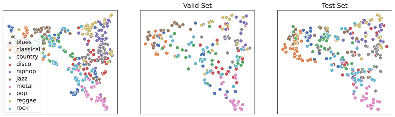<details> <summary>x30.png Details</summary>  ### Visual Description ## Scatter Plots: Music Genre Distribution Across Valid and Test Sets ### Overview The image contains three scatter plots labeled "Valid Set" and "Test Set," each displaying colored dots representing different music genres. A legend on the left maps colors to genres (e.g., blues = blue, classical = orange, etc.). The plots lack axis labels, but the spatial distribution of dots suggests clustering and variability in genre representation. ### Components/Axes - **Legend**: Positioned in the top-left corner of the first plot, with 10 genres listed: blues, classical, country, disco, hiphop, jazz, metal, pop, reggae, rock. Colors are assigned as follows: - Blues: Blue - Classical: Orange - Country: Green - Disco: Red - Hiphop: Purple - Jazz: Brown - Metal: Pink - Pop: Gray - Reggae: Yellow - Rock: Cyan - **Axes**: No explicit labels or scales are visible. The x- and y-axes appear to represent abstract dimensions (e.g., "genre similarity" or "data point density"), inferred from the clustering patterns. ### Detailed Analysis #### Valid Set - **Blues (Blue)**: Clustered in the top-left quadrant, with ~15–20 dots. - **Classical (Orange)**: Concentrated in the upper-middle region, ~10–12 dots. - **Country (Green)**: Spread across the middle-left, ~8–10 dots. - **Disco (Red)**: Scattered in the lower-middle, ~5–7 dots. - **Hiphop (Purple)**: Clustered in the upper-right, ~12–15 dots. - **Jazz (Brown)**: Dispersed in the middle, ~10–12 dots. - **Metal (Pink)**: Concentrated in the lower-right, ~8–10 dots. - **Pop (Gray)**: Scattered throughout, ~15–20 dots. - **Reggae (Yellow)**: Clustered in the upper-middle, ~6–8 dots. - **Rock (Cyan)**: Spread across the lower-right, ~10–12 dots. #### Test Set - **Blues (Blue)**: More dispersed, with ~10–12 dots in the top-left and middle regions. - **Classical (Orange)**: Clustered in the upper-middle, ~8–10 dots. - **Country (Green)**: Spread across the middle-left, ~7–9 dots. - **Disco (Red)**: Scattered in the lower-middle, ~4–6 dots. - **Hiphop (Purple)**: Clustered in the upper-right, ~10–12 dots. - **Jazz (Brown)**: Dispersed in the middle, ~9–11 dots. - **Metal (Pink)**: Concentrated in the lower-right, ~7–9 dots. - **Pop (Gray)**: Scattered throughout, ~12–15 dots. - **Reggae (Yellow)**: Clustered in the upper-middle, ~5–7 dots. - **Rock (Cyan)**: Spread across the lower-right, ~9–11 dots. ### Key Observations 1. **Clustering vs. Spread**: The Valid Set shows tighter clustering for genres like blues, hiphop, and pop, while the Test Set exhibits broader dispersion, suggesting greater variability in the test data. 2. **Genre Prevalence**: Pop and blues dominate both sets, with pop appearing most frequently in the Test Set. 3. **Outliers**: Disco and reggae have fewer data points in both sets, indicating underrepresentation. 4. **Spatial Trends**: In the Valid Set, blues and hiphop are tightly grouped, while in the Test Set, blues are more spread out, possibly reflecting a larger or more diverse dataset. ### Interpretation The scatter plots likely visualize the distribution of music genres in two distinct datasets (Valid and Test). The Valid Set’s clustering may indicate a smaller, more homogeneous sample, while the Test Set’s spread suggests broader coverage or higher diversity. The lack of axis labels limits quantitative analysis, but the visual patterns imply that the Test Set could be designed to test model generalization across varied genre representations. Outliers like disco and reggae highlight potential gaps in data collection or model training. </details> (b) MERT-330M RVQ-VAE Transformer Layer 22 Representations of GTZAN. 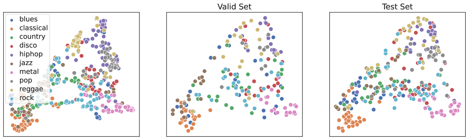<details> <summary>x31.png Details</summary>  ### Visual Description ## Scatter Plots: Music Genre Distribution in Valid and Test Sets ### Overview The image contains three scatter plots arranged horizontally. The leftmost plot includes a legend mapping 10 music genres to distinct colors (e.g., blues = blue, classical = orange, country = green). The middle and right plots are labeled "Valid Set" and "Test Set," respectively. All plots share identical axes (unlabeled x/y) and display overlapping clusters of colored points representing genre distributions. ### Components/Axes - **Legend**: Located in the top-left corner of the leftmost plot. - **Genres & Colors**: - Blues (blue), Classical (orange), Country (green), Disco (red), Hip-hop (purple), Jazz (brown), Metal (pink), Pop (gray), Reggae (yellow), Rock (light blue). - **Plots**: - **Valid Set** (middle): Scatter plot with overlapping genre clusters. - **Test Set** (right): Similar structure to Valid Set but with slightly different point distributions. - **Axes**: Unlabeled x and y axes in all plots. ### Detailed Analysis - **Genre Distribution**: - **Blues (blue)**: Concentrated in the lower-left region of all plots. - **Classical (orange)**: Dominates the bottom-left quadrant, with dense clusters in Valid and Test Sets. - **Country (green)**: Spreads diagonally from bottom-left to mid-right in Valid Set; more dispersed in Test Set. - **Disco (red)**: Clusters near the center-right in Valid Set; overlaps with pop (gray) in Test Set. - **Hip-hop (purple)**: Forms a dense cluster in the upper-right of Valid Set; less cohesive in Test Set. - **Jazz (brown)**: Scattered throughout but denser in the lower-middle region. - **Metal (pink)**: Concentrated in the upper-right of Test Set; sparse in Valid Set. - **Pop (gray)**: Widely distributed, with peaks in mid-right regions. - **Reggae (yellow)**: Small clusters near the top-center of Valid Set; absent in Test Set. - **Rock (light blue)**: Dominates the upper-right of Test Set; overlaps with hip-hop in Valid Set. ### Key Observations 1. **Cluster Overlap**: Genres like pop (gray) and disco (red) show significant overlap in Test Set, suggesting potential misclassification or shared features. 2. **Missing Data**: Reggae (yellow) appears only in Valid Set, indicating possible exclusion from the Test Set. 3. **Spatial Trends**: - Blues and classical consistently occupy the lower-left, while hip-hop and rock dominate upper-right regions. - Jazz and metal show less defined clustering, with points scattered across plots. ### Interpretation The scatter plots likely visualize a dimensionality reduction (e.g., PCA or t-SNE) of audio features, where each point represents a song/artist. The Valid and Test Sets exhibit similar genre distributions, implying the model generalizes well across subsets. However, the absence of reggae in the Test Set and overlapping clusters (e.g., pop/disco) suggest potential limitations in data balance or feature separation. The spatial trends align with genre characteristics (e.g., classical’s complexity vs. hip-hop’s rhythmic density), but further analysis of feature weights would clarify these relationships. </details> (c) MERT-330M RVQ-VAE Transformer Layer 23 Representations of GTZAN. 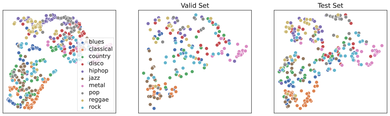<details> <summary>x32.png Details</summary>  ### Visual Description ## Scatter Plot: Music Genre Distribution Across Valid and Test Sets ### Overview The image contains three scatter plots visualizing the distribution of music genres across datasets. The first plot (unlabeled) appears to represent a training set, while the second and third plots are explicitly labeled "Valid Set" and "Test Set." Each plot uses color-coded dots to represent 10 distinct music genres, as defined in the legend. ### Components/Axes - **Legend**: Positioned on the left side of the image, mapping 10 genres to colors: - Blues (dark blue) - Classical (orange) - Country (green) - Disco (red) - Hiphop (purple) - Jazz (brown) - Metal (pink) - Pop (gray) - Reggae (yellow) - Rock (light blue) - **Plots**: - **Unlabeled Plot (Left)**: Likely the training set, with dense clusters of genres. - **Valid Set (Center)**: Intermediate distribution, showing partial clustering. - **Test Set (Right)**: More dispersed distribution, with overlapping genres. - **Axes**: No explicit axis labels or scales are visible, but the x- and y-axes span the same range across all plots. ### Detailed Analysis 1. **Unlabeled Plot (Training Set)**: - **Blues (dark blue)**: Clustered in the top-left quadrant. - **Classical (orange)**: Dense cluster in the bottom-left. - **Country (green)**: Spread across the middle. - **Disco (red)**: Concentrated in the middle-right. - **Hiphop (purple)**: Top-right cluster. - **Jazz (brown)**: Bottom-left, overlapping with classical. - **Metal (pink)**: Top-right, overlapping with hiphop. - **Pop (gray)**: Scattered throughout. - **Reggae (yellow)**: Top-left cluster. - **Rock (light blue)**: Bottom-right cluster. 2. **Valid Set (Center)**: - **Blues**: Less dense, spread toward the middle. - **Classical**: Still concentrated in the bottom-left but slightly dispersed. - **Country**: More dispersed, occupying the central region. - **Disco**: Spread toward the middle-right. - **Hiphop**: Top-right cluster, slightly smaller. - **Jazz**: Bottom-left, less overlapping with classical. - **Metal**: Top-right, smaller cluster. - **Pop**: Widely scattered. - **Reggae**: Top-left, smaller cluster. - **Rock**: Bottom-right, smaller cluster. 3. **Test Set (Right)**: - **Blues**: Dispersed across the top-left. - **Classical**: Spread from bottom-left to middle. - **Country**: Scattered throughout the middle. - **Disco**: Middle-right, less concentrated. - **Hiphop**: Top-right, smaller and more dispersed. - **Jazz**: Bottom-left, minimal overlap. - **Metal**: Top-right, highly dispersed. - **Pop**: Widely distributed. - **Reggae**: Top-left, minimal cluster. - **Rock**: Bottom-right, smaller and spread out. ### Key Observations - **Cluster Density**: The training set shows the most distinct genre clusters, while the test set exhibits significant overlap and dispersion. - **Genre-Specific Trends**: - **Metal (pink)** and **Hiphop (purple)** show the most pronounced clustering in the training set but become highly dispersed in the test set. - **Classical (orange)** and **Rock (light blue)** maintain some density in the training and valid sets but are more fragmented in the test set. - **Pop (gray)** remains the most uniformly distributed across all plots. - **Overlap**: Jazz (brown) and Classical (orange) overlap in the training set’s bottom-left, suggesting potential ambiguity in genre classification. ### Interpretation The data suggests that the model trained on the clustered training set may have overfit to specific genre distributions, as evidenced by the reduced separation in the valid and test sets. Genres like Metal and Hiphop, which are tightly grouped in the training data, become ambiguous in the test set, indicating potential challenges in generalization. The dispersion of genres in the test set highlights the importance of robust feature engineering to distinguish overlapping categories. Additionally, the consistent spread of Pop across all plots suggests it may serve as a baseline for comparison in model performance evaluation. </details> (d) MERT-330M RVQ-VAE Transformer Layer 24 Representations of GTZAN. Figure 6: Illustration of the MERT-330M RVQ-VAE Layer 21 to 24 Pre-trained Representations. ## Appendix D Ethics We have taken great care to ensure that our research adheres to ethical principles and guidelines in the codes of conduct. Specifically, we have not used personal user information in the experiments. Audio recordings are collected from open-access streaming services and open-source datasets, where the quality of the recordings varies among 16KHz, 24KHz, and 48KHz. The audio data would not be hosted and distributed. We believe that our work has the potential to contribute to positive social and scientific outcomes regarding the research of automatic music understanding.