2306.13063v2

# Can LLMs Express Their Uncertainty? An Empirical Evaluation of Confidence Elicitation in LLMs > Corresponding to: Miao Xiong (miao.xiong@u.nus.edu).Equal advising: bhooi@comp.nus.edu.sg, junxianh@cse.ust.hk Abstract Empowering large language models (LLMs) to accurately express confidence in their answers is essential for reliable and trustworthy decision-making. Previous confidence elicitation methods, which primarily rely on white-box access to internal model information or model fine-tuning, have become less suitable for LLMs, especially closed-source commercial APIs. This leads to a growing need to explore the untapped area of black-box approaches for LLM uncertainty estimation. To better break down the problem, we define a systematic framework with three components: prompting strategies for eliciting verbalized confidence, sampling methods for generating multiple responses, and aggregation techniques for computing consistency. We then benchmark these methods on two key tasks—confidence calibration and failure prediction—across five types of datasets (e.g., commonsense and arithmetic reasoning) and five widely-used LLMs including GPT-4 and LLaMA 2 Chat. Our analysis uncovers several key insights: 1) LLMs, when verbalizing their confidence, tend to be overconfident, potentially imitating human patterns of expressing confidence. 2) As model capability scales up, both calibration and failure prediction performance improve, yet still far from ideal performance. 3) Employing our proposed strategies, such as human-inspired prompts, consistency among multiple responses, and better aggregation strategies can help mitigate this overconfidence from various perspectives. 4) Comparisons with white-box methods indicate that while white-box methods perform better, the gap is narrow, e.g., 0.522 to 0.605 in AUROC. Despite these advancements, none of these techniques consistently outperform others, and all investigated methods struggle in challenging tasks, such as those requiring professional knowledge, indicating significant scope for improvement. We believe this study can serve as a strong baseline and provide insights for eliciting confidence in black-box LLMs. The code is publicly available at https://github.com/MiaoXiong2320/llm-uncertainty. 1 Introduction A key aspect of human intelligence lies in our capability to meaningfully express and communicate our uncertainty in a variety of ways (Cosmides & Tooby, 1996). Reliable uncertainty estimates are crucial for human-machine collaboration, enabling more rational and informed decision-making (Guo et al., 2017; Tomani & Buettner, 2021). Specifically, accurate confidence estimates of a model can provide valuable insights into the reliability of its responses, facilitating risk assessment and error mitigation (Kuleshov et al., 2018; Kuleshov & Deshpande, 2022), selective generation (Ren et al., 2022), and reducing hallucinations in natural language generation tasks (Xiao & Wang, 2021). In the existing literature, eliciting confidence from machine learning models has predominantly relied on white-box access to internal model information, such as token-likelihoods (Malinin & Gales, 2020; Kadavath et al., 2022) and associated calibration techniques (Jiang et al., 2021), as well as model fine-tuning (Lin et al., 2022). However, with the prevalence of large language models, these methods are becoming less suitable for several reasons: 1) The rise of closed-source LLMs with commercialized APIs, such as GPT-3.5 (OpenAI, 2021) and GPT-4 (OpenAI, 2023), which only allow textual inputs and outputs, lacking access to token-likelihoods or embeddings; 2) Token-likelihood primarily captures the model’s uncertainty about the next token (Kuhn et al., 2023), rather than the semantic probability inherent in textual meanings. For example, in the phrase “Chocolate milk comes from brown cows", every word fits naturally based on its surrounding words, but high individual token likelihoods do not capture the falsity of the overall statement, which requires examining the statement semantically, in terms of its claims; 3) Model fine-tuning demands substantial computational resources, which may be prohibitive for researchers with lower computational resources. Given these constraints, there is a growing need to explore black-box approaches for eliciting the confidence of LLMs in their answers, a task we refer to as confidence elicitation. Recognizing this research gap, our study aims to contribute to the existing knowledge from two perspectives: 1) explore black-box methods for confidence elicitation, and 2) conduct a comparative analysis to shed light on methods and directions for eliciting more accurate confidence. To achieve this, we define a systematic framework with three components: prompting strategies for eliciting verbalized confidence, sampling strategies for generating multiple responses, and aggregation strategies for computing the consistency. For each component, we devise a suite of methods. By integrating these components, we formulate a set of algorithms tailored for confidence elicitation. A comprehensive overview of the framework is depicted in Figure 1. We then benchmark these methods on two key tasks—confidence calibration and failure prediction—across five types of tasks (Commonsense, Arithmetic, Symbolic, Ethics and Professional Knowledge) and five widely-used LLMs, i.e., GPT-3 (Brown et al., 2020), GPT-3.5 (OpenAI, 2021), GPT-4, Vicuna (Chiang et al., 2023) and LLaMA 2 (Touvron et al., 2023b). Our investigation yields several observations: 1) LLMs tend to be highly overconfident when verbalizing their confidence, posing potential risks for the safe deployment of LLMs (§ 5.1). Intriguingly, the verbalized confidence values predominantly fall within the 80% to 100% range and are typically in multiples of 5, similar to how humans talk about confidence. In addition, while scaling model capacity leads to performance improvement, the results remain suboptimal. 2) Prompting strategies, inspired by patterns observed in human dialogues, can mitigate this overconfidence, but the improvement also diminishes as the model capacity scales up (§ 5.2). Furthermore, while the calibration error (e.g. ECE) can be significantly reduced using suitable prompting strategies, failure prediction still remains a challenge. 3) Our study on sampling and aggregation strategies indicates their effectiveness in improving failure prediction performance (§ 5.3). 4) A detailed examination of aggregation strategies reveals that they cater to specific performance metrics, i.e., calibration and failure prediction, and can be selected based on desired outcomes (§ 5.4). 5) Comparisons with white-box methods indicate that while white-box methods perform better, the gap is narrow, e.g., 0.522 to 0.605 in AUROC (§ B.1). Despite these insights, it is worth noting that the methods introduced herein still face challenges in failure prediction, especially with tasks demanding specialized knowledge (§ 6). This emphasizes the ongoing need for further research and development in confidence elicitation for LLMs. 2 Related Works Confidence Elicitation in LLMs. Confidence elicitation is the process of estimating LLM’s confidence in their responses without model fine-tuning or accessing internal information. Within this scope, Lin et al. (2022) introduced the concept of verbalized confidence that prompts LLMs to express confidence directly. However, they mainly focus on fine-tuning on specific datasets where the confidence is provided, and its zero-shot verbalized confidence is unexplored. Other approaches, like the external calibrator from Mielke et al. (2022), depend on internal model representations, which are often inaccessible. While Zhou et al. (2023) examines the impact of confidence, it does not provide direct confidence scores to users. Our work aligns most closely with the concurrent study by Tian et al. (2023), which mainly focuses on the use of prompting strategies. Our approach diverges by aiming to explore a broader method space, and propose a comprehensive framework for systematically evaluating various strategies and their integration. We also consider a wider range of models beyond those RLHF-LMs examined in concurrent research, thus broadening the scope of confidence elicitation. Our results reveal persistent challenges across more complex tasks and contribute to a holistic understanding of confidence elicitation. For a more comprehensive discussion of the related works, kindly refer to Appendix C. <details> <summary>x1.png Details</summary>  ### Visual Description ## Diagram: Prompt and Sampling Strategies ### Overview The image presents a diagram illustrating two different strategies for prompting and sampling from a "Black-box API," likely referring to a large language model (LLM). The diagram is divided into two sections, separated by a dashed line, representing two distinct approaches. The top section depicts a more general approach, while the bottom section shows a specific example with concrete values. ### Components/Axes **Top Section (General Approach):** * **Question:** A yellow rectangle labeled "Question" represents the initial input to the system. * **Prompt Strategy:** A blue rectangle labeled "Prompt Strategy" lists several prompting techniques: * Vanilla * Multi-step * Self-Probing * Top-K * CoT (Chain of Thought) * **Black-box API:** A black rectangle labeled "Black-box API" represents the LLM being used. It includes logos of AI models, including the 'AI' logo and the OpenAI logo. * **Sampling Strategy:** The phrase "Sampling Strategy" is above the Black-box API box. * **M Responses:** The system samples "M Responses" from the API. * **Response 1 ... Response K:** Yellow rectangles representing individual responses from the API. * **Aggregator:** A blue rectangle labeled "Aggregator" combines the multiple responses. * **Answer:** A yellow rectangle labeled "Answer" shows the final answer. * **Confidence:** A yellow rectangle labeled "Confidence" shows the confidence level associated with the answer. **Bottom Section (Specific Example):** * **Question:** A yellow cloud shape contains the question: "Q: How many prime numbers are in the list of 1,2,...,100?" * **Prompt:** A blue rectangle contains the prompt: "Q: \_\_\_\_ Provide the answer and your confidence in the answer." * **Black-box API:** A black rectangle labeled "Black-box API" represents the LLM. It includes the OpenAI logo. * **Self-Random:** A blue rectangle labeled "Self-Random" is above the Black-box API box. * **3 Responses:** The system samples "3 Responses" from the API. * **Responses:** Three yellow rectangles show the individual responses: * "Answer: 100; Confidence: 100%" * "Answer: 20; Confidence: 90%" * "Answer: 25; Confidence: 80%" * **Avg-Conf Aggregation:** A blue rectangle labeled "Avg-Conf Aggregation" combines the responses. * **Answer:** A yellow rectangle labeled "Answer: 100" shows the final answer. * **Confidence:** A yellow rectangle labeled "Confidence: 37%" shows the confidence level associated with the answer. ### Detailed Analysis or ### Content Details **Flow:** * In the top section, the "Question" is fed into the "Prompt Strategy," which then interacts with the "Black-box API" to generate "M Responses." These responses are aggregated to produce a final "Answer" and "Confidence" score. * In the bottom section, a specific question about prime numbers is used. The prompt asks for both the answer and the confidence level. The "Black-box API" generates 3 responses, which are then aggregated using "Avg-Conf Aggregation" to produce a final answer and confidence score. **Values:** * In the bottom section, the individual responses have the following values: * Response 1: Answer = 100, Confidence = 100% * Response 2: Answer = 20, Confidence = 90% * Response 3: Answer = 25, Confidence = 80% * The final aggregated result in the bottom section is: * Answer = 100 * Confidence = 37% ### Key Observations * The diagram highlights two different approaches to interacting with an LLM: a general approach with configurable prompting and sampling strategies, and a specific example with a concrete question and a fixed number of responses. * The aggregation method in the bottom section ("Avg-Conf Aggregation") appears to be averaging the confidence scores of the individual responses. (100% + 90% + 80%) / 3 = 90%. However, the final confidence is 37%, which suggests that the aggregation method is more complex than a simple average. * The final answer in the bottom section is 100, which matches one of the individual responses. ### Interpretation The diagram illustrates how different prompting and sampling strategies can be used to interact with LLMs. The specific example in the bottom section demonstrates that even when individual responses have high confidence levels, the aggregated result may have a significantly lower confidence level. This suggests that averaging confidence scores may not be a reliable way to assess the overall confidence in the final answer. The discrepancy between the individual confidence scores and the final confidence score highlights the challenges of working with LLMs and the need for more sophisticated aggregation methods. The diagram also suggests that the choice of prompt and sampling strategy can significantly impact the quality and reliability of the results. 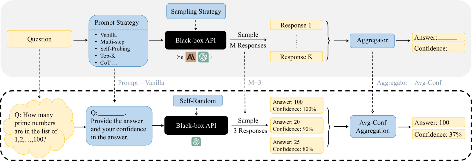</details> Figure 1: An Overview and example of Confidence Elicitation framework, which consists of three components: prompt, sampling and aggregator. By integrating distinct strategies from each component, we can devise different algorithms, e.g., Top-K (Tian et al., 2023) is formulated using Top-K prompt, self-random sampling with $M=1$ , and Avg-Conf aggregation. Given an input question, we first choose a suitable prompt strategy, e.g., the vanilla prompt used here. Next, we determine the number of samples to generate ( $M=3$ here) and sampling strategy, and then choose an aggregator based on our preference (e.g. focus more on improving calibration or failure prediction) to compute confidences in its potential answers. The highest confident answer is selected as the final output. 3 Exploring Black-box Framework for Confidence Elicitation In our pursuit to explore black-box approaches for eliciting confidence, we investigated a range of methods and discovered that they can be encapsulated within a unified framework. This framework, with its three pivotal components, offers a variety of algorithmic choices that combine to create diverse algorithms with different benefits for confidence elicitation. In our later experimental section (§ 5), we will analyze our proposed strategies within each component, aiming to shed light on the best practices for eliciting confidence in black-box LLMs. 3.1 Motivation of The Framework Prompting strategy. The key question we aim to answer here is: in a black-box setting, what form of model inputs and outputs lead to the most accurate confidence estimates? This parallels the rich study in eliciting confidences from human experts: for example, patients often inquire of doctors about their confidence in the potential success of a surgery. We refer to this goal as verbalized confidence, and inspired by strategies for human elicitation, we design a series of human-inspired prompting strategies to elicit the model’s verbalized confidence. We then unify these prompting strategies as a building block of our framework (§ 3.2). In addition, beyond its simplicity, this approach also offers an extra benefit over model’s token-likelihood: the verbalized confidence is intrinsically tied to the semantic meaning of the answer instead of its syntactic or lexical form (Kuhn et al., 2023). Sampling and Aggregation. In addition to the direct insights from model outputs, the variance observed among multiple responses for a given question offers another valuable perspective on model confidence. This line of thought aligns with the principle extensively explored in prior white-box access uncertainty estimation methodologies for classification (Gawlikowski et al., 2021), such as MCDropout (Gal & Ghahramani, 2016) and Deep Ensemble (Lakshminarayanan et al., 2017). The challenges in adapting ensemble-based methods lie in two critical components: 1) the sampling strategy, i.e., how to sample multiple responses from the model’s answer distribution, and 2) the aggregation strategy, i.e., how to aggregate these responses to yield the final answer and its associated confidence. To optimally harness both textual output and response variance, we have integrated them within a unified framework. Table 1: Illustration of the prompting strategy (the complete prompt in Appendix F). To help models understand the concept of confidence, we also append the explanation “Note: The confidence indicates how likely you think your answer is true." to every prompt. | Vanilla CoT Self-Probing | Read the question, provide your answer, and your confidence in this answer. Read the question, analyze step by step, provide your answer and your confidence in this answer. Question: […] Possible Answer: […] Q: How likely is the above answer to be correct? Analyze the possible answer, provide your reasoning concisely, and give your confidence in this answer. | | --- | --- | | Multi-Step | Read the question, break down the problem into K steps, think step by step, give your confidence in each step, and then derive your final answer and your confidence in this answer. | | Top-K | Provide your $K$ best guesses and the probability that each is correct (0% to 100%) for the following question. | 3.2 Prompting Strategy Drawing inspiration from patterns observed in human dialogues, we design a series of human-inspired prompting strategies to tackle challenges, e.g., overconfidence, that are inherent in the vanilla version of verbalized confidence. See Table 1 for an overview of these prompting strategies and Appendix F for complete prompts. CoT. Considering that a better comprehension of a problem can lead to a more accurate understanding of one’s certainty, we adopt a reasoning-augmented prompting strategy. In this paper, we use zero-shot Chain-of-Thought, CoT (Kojima et al., 2022) for its proven efficacy in inducing reasoning processes and improving model accuracy across diverse datasets. Alternative strategies such as plan-and-solve (Wang et al., 2023) can also be used. Self-Probing. A common observation of humans is that they often find it easier to identify errors in others’ answers than in their own, as they can become fixated on a particular line of thinking, potentially overlooking mistakes. Building on this assumption, we investigate if a model’s uncertainty estimation improves when given a question and its answer, then asked, “How likely is the above answer to be correct"? The procedure involves generating the answer in one chat session and obtaining its verbalized confidence in another independent chat session. Multi-Step. Our preliminary study shows that LLMs tend to be overconfident when verbalizing their confidence (see Figure 2). To address this, we explore whether dissecting the reasoning process into steps and extracting the confidence of each step can alleviate the overconfidence. The rationale is that understanding each reasoning step’s confidence could help the model identify potential inaccuracies and quantify their confidence more accurately. Specifically, for a given question, we prompt models to delineate their reasoning process into individual steps $S_{i}$ and evaluate their confidence in the correctness of this particular step, denoted as $C_{i}$ . The overall verbalized confidence is then derived by aggregating the confidence of all steps: $C_{\text{multi-step}}=\prod_{i=1}^{n}C_{i}$ , where $n$ represents the total number of reasoning steps. Top-K. Another way to alleviate overconfidence is to realize the existence of multiple possible solutions or answers, which acts as a normalization for the confidence distribution. Motivated by this, Top-K (Tian et al., 2023) prompts LLMs to generate the top $K$ guesses and their corresponding confidence for a given question. 3.3 Sampling Strategy Several methods can be employed to elicit multiple responses of the same question from the model: 1) Self-random, leveraging the model’s inherent randomness by inputting the same prompt multiple times. The temperature, an adjustable parameter, can be used to calibrate the predicted token distribution, i.e., adjust the diversity of the sampled answers. An alternative choice is to introduce perturbations in the questions: 2) Prompting, by paraphrasing the questions in different ways to generate multiple responses. 3) Misleading, feeding misleading cues to the model, e.g.,“I think the answer might be …". This method draws inspiration from human behaviors: when confident, individuals tend to stick to their initial answers despite contrary suggestions; conversely, when uncertain, they are more likely to waver or adjust their responses based on misleading hints. Building on this observation, we evaluate the model’s response to misleading information to gauge its uncertainty. See Table 11 for the complete prompts. 3.4 Aggregation Strategy Consistency. A natural idea of aggregating different answers is to measure the degree of agreement among the candidate outputs and integrate the inherent uncertainty in the model’s output. For any given question and an associated answer $\tilde{Y}$ , we sample a set of candidate answers $\hat{Y}_{i}$ , where $i∈\{1,...,M\}$ . The agreement between these candidate responses and the original answer then serves as a measure of confidence, computed as follows: $$ C_{\operatorname{consistency}}=\frac{1}{M}\sum_{i=1}^{M}\mathbb{I}\{\hat{Y}_{i% }=\tilde{Y}\}. \tag{1} $$ Avg-Conf. The previous aggregation method does not utilize the available information of verbalized confidence. It is worth exploring the potential synergy between these uncertainty indicators, i.e., whether the verbalized confidence and the consistency between answers can complement one another. For any question and an associated answer $\tilde{Y}$ , we sample a candidate set $\{\hat{Y}_{1},...\hat{Y}_{M}\}$ with their corresponding verbalized confidence $\{C_{1},...C_{M}\}$ , and compute the confidence as follows: $$ C_{\operatorname{conf}}=\frac{\sum_{i=1}^{M}\mathbb{I}\{\hat{Y}_{i}=\tilde{Y}% \}\times C_{i}}{\sum_{i=1}^{M}C_{i}}. \tag{2} $$ Pair-Rank. This aggregation strategy is tailored for responses generated using the Top-K prompt, as it mainly utilizes the ranking information of the model’s Top-K guesses. The underlying assumption is that the model’s ranking between two options may be more accurate than the verbalized confidence it provides, especially given our observation that the latter tends to exhibit overconfidence. Given a question with $N$ candidate responses, the $i\text{-th}$ response consists of $K$ sequentially ordered answers, denoted as $\mathcal{S}^{(i)}_{K}=(S_{1}^{(i)},S_{2}^{(i)},...,S_{K}^{(i)})$ . Let $\mathcal{A}$ represent the set of unique answers across all $N$ responses, where $M$ is the total number of distinct answers. The event where the model ranks answer $S_{u}$ above $S_{v}$ (i.e., $S_{u}$ appears before $S_{v}$ ) in its $i$ -th generation is represented as $(S_{u}\stackrel{{\scriptstyle\scriptstyle(i)}}{{\succ}}S_{v})$ . In contexts where the generation is implicit, this is simply denoted as $(S_{u}\succ S_{v})$ . Let $E_{uv}^{(i)}$ be the event where at least one of $S_{u}$ and $S_{v}$ appears in the $i$ -th generation. Then the probability of $(S_{u}\succ S_{v})$ , conditional on $E_{uv}^{(i)}$ and a categorical distribution $P$ , is expressed as $\mathbb{P}(S_{u}\succ S_{v}|P,E_{uv}^{(i)})$ . We then utilize a (conditional) maximum likelihood estimation (MLE) inspired approach to derive the categorical distribution $P$ that most accurately reflects these ranking events of all the $M$ responses: $$ \min_{P}{\color[rgb]{0,0,0}-}\sum_{i=1}^{N}\sum_{S_{u}\in\mathcal{A}}\sum_{S_{% v}\in\mathcal{A}}\mathbb{I}\left\{S_{u}\stackrel{{\scriptstyle\scriptstyle(i)}% }{{\succ}}S_{v}\right\}\cdot\log\mathbb{P}\left(S_{u}\succ S_{v}\mid P,E_{uv}^% {(i)}\right)\quad\text{subject to}\sum_{S_{u}\in\mathcal{A}}P\left(S_{u}\right% )=1 \tag{3} $$ **Proposition 3.1** *Suppose the Top-K answers are drawn from a categorical distribution $P$ without replacement. Define the event $(S_{u}\succ S_{v})$ to indicate that the realization $S_{u}$ is observed before $S_{v}$ in the $i\text{-th}$ draw without replacement. Under this setting, the conditional probability is given by: $$ \mathbb{P}\left(S_{u}\succ S_{v}\mid P,E_{uv}^{(i)}\right)=\frac{P(S_{u})}{P(S% _{u})+P(S_{v})} $$ The optimization objective to minimize the expected loss is then: $$ \min_{P}{\color[rgb]{0,0,0}-}\sum_{i=1}^{N}\sum_{S_{u}\in\mathcal{A}}\sum_{S_{% v}\in\mathcal{A}}\mathbb{I}\left\{S_{u}\stackrel{{\scriptstyle\scriptstyle(i)}% }{{\succ}}S_{v}\right\}\cdot\log\frac{P(S_{u})}{P(S_{u})+P(S_{v})}\quad\text{s% .t.}\sum_{S_{u}\in\mathcal{A}}P\left(S_{u}\right)=1 \tag{4} $$* To address this constrained optimization problem, we first introduce a change of variables by applying the softmax function to the unbounded domain. This transformation inherently satisfies the simplex constraints, converting our problem into an unconstrained optimization setting. Subsequently, optimization techniques such as gradient descent can be used to obtain the categorical distribution. 4 Experiment Setup Datasets. We evaluate the quality of confidence estimates across five types of reasoning tasks: 1) Commonsense Reasoning on two benchmarks, Sports Understanding (SportUND) (Kim, 2021) and StrategyQA (Geva et al., 2021) from BigBench (Ghazal et al., 2013); 2) Arithmetic Reasoning on two math problems, GSM8K (Cobbe et al., 2021) and SVAMP (Patel et al., 2021); 3) Symbolic Reasoning on two benchmarks, Date Understanding (DateUnd) (Wu & Wang, 2021) and Object Counting (ObjectCou) (Wang et al., 2019) from BigBench; 4) tasks requiring Professional Knowledge, such as Professional Law (Prf-Law) from MMLU (Hendrycks et al., 2021); 5) tasks that require Ethical Knowledge, e.g., Business Ethics (Biz-Ethics) from MMLU (Hendrycks et al., 2021). Models We incorporate a range of widely used LLMs of different scales, including Vicuna 13B (Chiang et al., 2023), GPT-3 175B (Brown et al., 2020), GPT-3.5-turbo (OpenAI, 2021), GPT-4 (OpenAI, 2023) and LLaMA 2 70B (Touvron et al., 2023b). Evaluation Metrics. To evaluate the quality of confidence outputs, two orthogonal tasks are typically employed: calibration and failure prediction (Naeini et al., 2015; Yuan et al., 2021; Xiong et al., 2022). Calibration evaluates how well a model’s expressed confidence aligns with its actual accuracy: ideally, samples with an 80% confidence should have an accuracy of 80%. Such well-calibrated scores are crucial for applications including risk assessment. On the other hand, failure prediction gauges the model’s capacity to assign higher confidence to correct predictions and lower to incorrect ones, aiming to determine if confidence scores can effectively distinguish between correct and incorrect predictions. In our study, we employ Expected Calibration Error (ECE) for calibration evaluation and Area Under the Receiver Operating Characteristic Curve (AUROC) for gauging failure prediction. Given the potential imbalance from varying accuracy levels, we also introduce AUPRC-Positive (PR-P) and AUPRC-Negative (PR-N) metrics to emphasize whether the model can identify incorrect and correct samples, respectively. Further details on datasets, models, metrics, and implementation can be found in Appendix E. <details> <summary>x2.png Details</summary>  ### Visual Description ## Chart Type: Model Confidence Histograms and Calibration Plots ### Overview The image presents a set of histograms and calibration plots comparing the confidence levels of four different language models: GPT-3, GPT-3.5, GPT-4, and Vicuna. Each model has a histogram showing the distribution of its confidence scores for correct and incorrect answers, along with a calibration plot displaying the accuracy within each confidence bin. The plots are arranged in a 2x4 grid, with histograms in the top row and calibration plots in the bottom row. ### Components/Axes **Histograms (Top Row):** * **Title:** Each histogram is titled with the model name (GPT-3, GPT-3.5, GPT-4, Vicuna) and performance metrics (ACC, AUROC, ECE). * **Y-axis:** "Count" - Represents the number of predictions falling into each confidence bin. * **X-axis:** "Confidence (%)" - Represents the confidence level of the model, ranging from 50% to 100% in increments of 10%. * **Legend (Top-Left of each histogram):** * Red: "wrong answer" * Blue: "correct answer" **Calibration Plots (Bottom Row):** * **Y-axis:** "Accuracy Within Bin" - Represents the accuracy of the model for predictions within a specific confidence bin, ranging from 0.0 to 1.0. * **X-axis:** "Confidence" - Represents the confidence level, ranging from 0.0 to 1.0. * **Diagonal Dashed Line:** Represents perfect calibration (accuracy equals confidence). ### Detailed Analysis **GPT-3:** * **Histogram:** * ACC 0.15 / AUROC 0.51 / ECE 0.83 * The "wrong answer" (red) bar is very high at 100% confidence. * A small "correct answer" (blue) bar is present at 80% confidence. * **Calibration Plot:** * Accuracy Within Bin is approximately 0.1 for a confidence of 0.8. * Accuracy Within Bin is approximately 0.1 for a confidence of 1.0. * The model is poorly calibrated, with accuracy significantly lower than confidence. **GPT-3.5:** * **Histogram:** * ACC 0.28 / AUROC 0.65 / ECE 0.66 * The "wrong answer" (red) bar is high at 100% confidence. * A significant "correct answer" (blue) bar is present at 90-100% confidence. * **Calibration Plot:** * Accuracy Within Bin is approximately 0.7 for a confidence of 0.8. * Accuracy Within Bin is approximately 0.8 for a confidence of 0.9. * Accuracy Within Bin is approximately 0.9 for a confidence of 1.0. * The model shows better calibration than GPT-3, but still overconfident. **GPT-4:** * **Histogram:** * ACC 0.47 / AUROC 0.66 / ECE 0.51 * The "wrong answer" (red) bar is high at 100% confidence. * A significant "correct answer" (blue) bar is present at 90-100% confidence. * **Calibration Plot:** * Accuracy Within Bin is approximately 0.8 for a confidence of 0.8. * Accuracy Within Bin is approximately 0.9 for a confidence of 0.9. * Accuracy Within Bin is approximately 0.9 for a confidence of 1.0. * The model shows better calibration than GPT-3, and GPT-3.5, but still overconfident. **Vicuna:** * **Histogram:** * ACC 0.02 / AUROC 0.46 / ECE 0.77 * The "wrong answer" (red) bar is very high at 80% confidence. * A small "correct answer" (blue) bar is present at 80% confidence. * **Calibration Plot:** * Accuracy Within Bin is approximately 0.0 for a confidence of 0.4. * Accuracy Within Bin is approximately 0.0 for a confidence of 0.5. * Accuracy Within Bin is approximately 0.0 for a confidence of 0.6. * Accuracy Within Bin is approximately 0.0 for a confidence of 0.7. * Accuracy Within Bin is approximately 0.0 for a confidence of 0.8. * Accuracy Within Bin is approximately 0.0 for a confidence of 0.9. * Accuracy Within Bin is approximately 0.0 for a confidence of 1.0. * The model is poorly calibrated, with accuracy significantly lower than confidence. ### Key Observations * All models tend to be overconfident, especially at higher confidence levels. * GPT-4 exhibits the best calibration among the four models, as its accuracy within each bin is closest to the confidence level. * GPT-3 and Vicuna are poorly calibrated, with accuracy lagging significantly behind confidence. * The histograms show that most predictions cluster at high confidence levels, particularly for incorrect answers. ### Interpretation The data suggests that while these language models can achieve high confidence in their predictions, their confidence is not always well-aligned with their actual accuracy. This is a common issue in machine learning, known as overconfidence. The calibration plots provide a visual representation of this phenomenon, highlighting the discrepancy between predicted confidence and actual accuracy. GPT-4 demonstrates better calibration compared to the other models, indicating that its confidence scores are more reliable. The high concentration of incorrect answers at high confidence levels suggests that these models may struggle with certain types of questions or scenarios, leading to overconfident but ultimately wrong predictions. The ECE (Expected Calibration Error) values, given in the titles, quantify the calibration error, with lower values indicating better calibration. 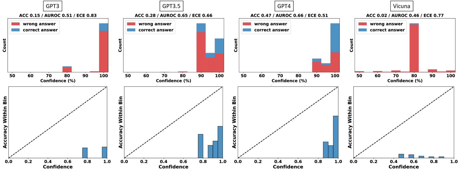</details> Figure 2: Empirical distribution (First row) and reliability diagram (Second row) of vanilla verbalized confidence across four models on GSM8K. The prompt used is in Table 14. From this figure, we can observe that 1) the confidence levels primarily range between 80% and 100%, often in multiples of 5; 2) the accuracy within each bin is much lower than its corresponding confidence, indicating significant overconfidence. 5 Evaluation and Analysis To provide insights on the best practice for eliciting confidence, we systematically examine each component (see Figure 1) of the confidence elicitation framework (§ 3). We test the performance on eight datasets of five different reasoning types and five commonly used models (see § 4), and yield the following key findings. 5.1 LLMs tend to be overconfident when verbalizing their confidence The distribution of verbalized confidences mimics how humans talk about confidence. To examine model’s capacity to express verbalized confidence, we first visualize the distribution of confidence in Figure 2. Detailed results on other datasets and models are provided in Appendix Figure 5. Notably, the models tend to have high confidence for all samples, appearing as multiples of 5 and with most values ranging between the 80% to 100% range, which is similar to the patterns identified in the training corpus for GPT-like models as discussed by Zhou et al. (2023). Such behavior suggests that models might be imitating human expressions when verbalizing confidence. Calibration and failure prediction performance improve as model capacity scales. The comparison of the performance of various models (Table 2) reveals a trend: as we move from GPT-3, Vicuna, GPT-3.5 to GPT-4, with the increase of model accuracy, there is also a noticeable decrease in ECE and increase in AUROC, e.g., approximate 22.2% improvement in AUROC from GPT-3 to GPT-4. Vanilla verbalized confidence exhibits significant overconfidence and poor failure prediction, casting doubts on its reliability. Table 2 presents the performance of vanilla verbalized confidence across five models and eight tasks. According to the criteria given in Srivastava et al. (2023), GPT-3, GPT-3.5, and Vicuna exhibit notably high ECE values, e.g., the average ECE exceeding 0.377, suggesting that the verbalized confidence of these LLMs are poorly calibrated. While GPT-4 displays lower ECE, its AUROC and AUPRC-Negative scores remain suboptimal, with an average AUROC of merely 62.7%—close to the 50% random guess threshold—highlighting challenges in distinguishing correct from incorrect predictions. Table 2: Vanilla Verbalized Confidence of 4 models and 8 datasets (metrics are given by $× 10^{2}$ ). Abbreviations are used: Date (Date Understanding), Count (Object Counting), Sport (Sport Understanding), Law (Professional Law), Ethics (Business Ethics). ECE > 0.25, AUROC, AUPRC-Positive, AUPRC-Negative < 0.6 denote significant deviation from ideal performance. Significant deviations in averages are highlighted in red. The prompt used is in Table 14. | ECE $\downarrow$ Vicuna LLaMA 2 | GPT-3 76.0 71.8 | 82.7 70.7 36.4 | 35.0 17.0 38.5 | 82.1 45.3 58.0 | 52.0 42.5 26.2 | 41.8 37.5 38.8 | 42.0 45.2 42.2 | 47.8 34.6 36.5 | 32.3 46.1 43.6 | 52.0 | | --- | --- | --- | --- | --- | --- | --- | --- | --- | --- | --- | | GPT-3.5 | 66.0 | 22.4 | 47.0 | 47.1 | 26.0 | 25.1 | 44.3 | 23.4 | 37.7 | | | GPT-4 | 31.0 | 10.7 | 18.0 | 26.8 | 16.1 | 15.4 | 17.3 | 8.5 | 18.0 | | | ROC $\uparrow$ | GPT3 | 51.2 | 51.7 | 50.2 | 50.0 | 49.3 | 55.3 | 46.5 | 56.1 | 51.3 | | Vicuna | 52.1 | 46.3 | 53.7 | 53.1 | 50.9 | 53.6 | 52.6 | 57.5 | 52.5 | | | LLaMA 2 | 58.8 | 52.1 | 71.4 | 51.3 | 56.0 | 48.5 | 50.5 | 62.4 | 56.4 | | | GPT-3.5 | 65.0 | 63.2 | 57.0 | 54.1 | 52.8 | 43.2 | 50.5 | 55.2 | 55.1 | | | GPT4 | 81.0 | 56.7 | 68.0 | 52.0 | 55.3 | 60.0 | 60.9 | 68.0 | 62.7 | | | PR-N $\uparrow$ | GPT-3 | 85.0 | 37.3 | 82.2 | 52.0 | 42.0 | 46.4 | 51.2 | 41.2 | 54.7 | | Vicuna | 96.4 | 87.9 | 34.9 | 65.4 | 53.8 | 51.5 | 75.3 | 70.9 | 67.0 | | | LLaMA 2 | 92.6 | 57.4 | 88.3 | 59.6 | 38.2 | 40.6 | 61.0 | 58.3 | 62.0 | | | GPT-3.5 | 79.0 | 33.9 | 64.0 | 51.2 | 35.7 | 30.5 | 54.8 | 35.5 | 48.1 | | | GPT-4 | 65.0 | 15.8 | 26.0 | 28.9 | 26.6 | 31.5 | 40.0 | 39.5 | 34.2 | | | PR-P $\uparrow$ | GPT-3 | 15.5 | 65.5 | 17.9 | 48.0 | 57.6 | 59.0 | 45.4 | 66.1 | 46.9 | | Vicuna | 4.10 | 11.0 | 69.1 | 39.1 | 47.5 | 52.0 | 27.2 | 38.8 | 36.1 | | | LLaMA 2 | 11.9 | 46.3 | 46.6 | 41.4 | 68.6 | 58.3 | 39.2 | 65.0 | 47.2 | | | GPT-3.5 | 38.0 | 81.3 | 57.0 | 54.4 | 67.2 | 67.5 | 45.8 | 70.5 | 60.2 | | | GPT-4 | 57.0 | 90.1 | 88.0 | 73.8 | 78.6 | 79.3 | 73.4 | 87.2 | 78.4 | | 5.2 Human-inspired Prompting Strategies Partially Reduce Overconfidence Human-inspired prompting strategies improve model accuracy and calibration, albeit with diminishing returns in advanced models like GPT-4. As illustrated in Figure 3, we compare the performance of five prompting strategies across five datasets on GPT-3.5 and GPT-4. Analyzing the average ECE, AUROC, and their respective performances within each dataset, human-inspired strategies offer consistent improvements in accuracy and calibration over the vanilla baseline, with modest advancements in failure prediction. No single prompting strategy consistently outperforms the others. Figure 3 suggests that there is no single strategy that can consistently outperform the others across all the datasets and models. By evaluating the average rank and performance enhancement for each method over five task types, we find that Self-Probing maintains the most consistent advantage over the baseline on GPT-4, while Top-K emerges as the top performer on GPT-3.5. <details> <summary>x3.png Details</summary>  ### Visual Description ## Bar Charts: Model Performance Comparison ### Overview The image contains four bar charts comparing the performance of different models (GPT-3.5 and GPT-4) across several tasks. The charts are arranged in a 2x2 grid. The left two charts display the Expected Calibration Error (ECE), while the right two display the Area Under the Receiver Operating Characteristic curve (AUROC). Each chart compares different prompting strategies: vanilla, self_evaluate, cot (Chain of Thought), multistep, and topk. The x-axis represents different tasks (DateUnd, Biz-Ethics, GSM8K, Prf-Law, StrategyQA) and an average across all tasks. ### Components/Axes * **Titles:** * Top-left: GPT-3.5: ECE ↓ * Top-middle-left: GPT-4: ECE ↓ * Top-middle-right: GPT-3.5: AUROC ↑ * Top-right: GPT-4: AUROC ↑ * **Y-axes:** * Left two charts: "ece", scale from 0.0 to 0.7 * Right two charts: "auroc", scale from 0.0 to 1.0 * **X-axes:** * All charts: Categories: DateUnd, Biz-Ethics, GSM8K, Prf-Law, StrategyQA, average * **Legends:** (Located in the top-middle-left chart, applies to all charts) * `mean ece` (black dashed line in the ECE charts) or `mean auroc` (black solid line in the AUROC charts) * `vanilla` (blue) * `self_evaluate` (orange) * `cot` (green) * `multistep` (red) * `topk` (purple) ### Detailed Analysis **Chart 1: GPT-3.5: ECE ↓** * Trend: ECE varies across tasks and prompting strategies. * DateUnd: vanilla ~0.47, self_evaluate ~0.27, cot ~0.24, multistep ~0.26, topk ~0.25 * Biz-Ethics: vanilla ~0.30, self_evaluate ~0.28, cot ~0.29, multistep ~0.24, topk ~0.12 * GSM8K: vanilla ~0.65, self_evaluate ~0.38, cot ~0.10, multistep ~0.43, topk ~0.20 * Prf-Law: vanilla ~0.43, self_evaluate ~0.28, cot ~0.35, multistep ~0.27, topk ~0.40 * StrategyQA: vanilla ~0.35, self_evaluate ~0.30, cot ~0.25, multistep ~0.22, topk ~0.15 * average: vanilla ~0.42, self_evaluate ~0.30, cot ~0.25, multistep ~0.28, topk ~0.22 * Mean ECE (black dashed line): ~0.29 **Chart 2: GPT-4: ECE ↓** * Trend: ECE is generally lower than GPT-3.5, indicating better calibration. * DateUnd: vanilla ~0.15, self_evaluate ~0.09, cot ~0.07, multistep ~0.14, topk ~0.14 * Biz-Ethics: vanilla ~0.40, self_evaluate ~0.35, cot ~0.25, multistep ~0.25, topk ~0.20 * GSM8K: vanilla ~0.15, self_evaluate ~0.15, cot ~0.10, multistep ~0.22, topk ~0.05 * Prf-Law: vanilla ~0.18, self_evaluate ~0.16, cot ~0.17, multistep ~0.15, topk ~0.12 * StrategyQA: vanilla ~0.15, self_evaluate ~0.15, cot ~0.15, multistep ~0.15, topk ~0.10 * average: vanilla ~0.20, self_evaluate ~0.18, cot ~0.15, multistep ~0.18, topk ~0.12 * Mean ECE (black dashed line): ~0.15 **Chart 3: GPT-3.5: AUROC ↑** * Trend: AUROC varies across tasks and prompting strategies. * DateUnd: vanilla ~0.62, self_evaluate ~0.61, cot ~0.58, multistep ~0.72, topk ~0.73 * Biz-Ethics: vanilla ~0.60, self_evaluate ~0.60, cot ~0.57, multistep ~0.59, topk ~0.59 * GSM8K: vanilla ~0.52, self_evaluate ~0.50, cot ~0.53, multistep ~0.51, topk ~0.60 * Prf-Law: vanilla ~0.60, self_evaluate ~0.59, cot ~0.58, multistep ~0.59, topk ~0.70 * StrategyQA: vanilla ~0.60, self_evaluate ~0.59, cot ~0.57, multistep ~0.59, topk ~0.60 * average: vanilla ~0.58, self_evaluate ~0.57, cot ~0.57, multistep ~0.58, topk ~0.64 * Mean AUROC (black solid line): ~0.59 **Chart 4: GPT-4: AUROC ↑** * Trend: AUROC is generally higher than GPT-3.5, indicating better performance. * DateUnd: vanilla ~0.72, self_evaluate ~0.73, cot ~0.72, multistep ~0.56, topk ~0.78 * Biz-Ethics: vanilla ~0.78, self_evaluate ~0.79, cot ~0.75, multistep ~0.57, topk ~0.65 * GSM8K: vanilla ~0.50, self_evaluate ~0.50, cot ~0.50, multistep ~0.50, topk ~0.50 * Prf-Law: vanilla ~0.65, self_evaluate ~0.64, cot ~0.63, multistep ~0.63, topk ~0.63 * StrategyQA: vanilla ~0.65, self_evaluate ~0.64, cot ~0.63, multistep ~0.63, topk ~0.63 * average: vanilla ~0.66, self_evaluate ~0.66, cot ~0.65, multistep ~0.58, topk ~0.64 * Mean AUROC (black solid line): ~0.63 ### Key Observations * GPT-4 generally outperforms GPT-3.5 in both calibration (lower ECE) and accuracy (higher AUROC). * The "vanilla" prompting strategy often performs comparably to or better than more complex strategies like "self_evaluate" and "cot" for GPT-4. * The "topk" prompting strategy often achieves higher AUROC scores, especially for GPT-3.5. * GSM8K consistently shows lower AUROC scores compared to other tasks, particularly for GPT-4. * The ECE scores for GPT-4 are significantly lower than those for GPT-3.5, indicating better calibration. ### Interpretation The data suggests that GPT-4 is a more reliable and accurate model than GPT-3.5 across the tasks evaluated. The lower ECE values for GPT-4 indicate that its confidence in its predictions is better aligned with its actual accuracy. The higher AUROC values suggest that GPT-4 is better at distinguishing between positive and negative examples. The effectiveness of different prompting strategies varies between the two models. While complex strategies like "self_evaluate" and "cot" might be expected to improve performance, the "vanilla" strategy often performs well, especially for GPT-4. This could indicate that GPT-4 is better at understanding and responding to simple prompts. The consistently lower AUROC scores for GSM8K suggest that this task is particularly challenging for both models. This could be due to the nature of the task itself or the way the data is structured. 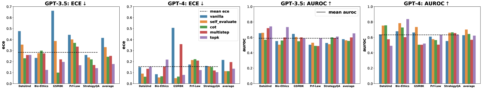</details> Figure 3: Comparative analysis of 5 prompting strategies over 5 datasets for 2 models (GPT-3.5 and GPT-4). The ‘average’ bar represents the mean ECE for a given prompting strategy across datasets. The ‘mean ECE’ line is the average across all strategies and datasets. AUROC is calculated in a similar manner. The accuracy comparison is shown in Appendix B.4. While ECE can be effectively reduced using suitable prompting strategies, failure prediction still remains a challenge. Comparing the average calibration performance across datasets (‘mean ece’ lines) and the average failure prediction performance (‘mean auroc’), we find that while we can reduce ECE with the right prompting strategy, the model’s failure prediction capability is still limited, i.e., close to the performance of random guess (AUROC=0.5). A closer look at individual dataset performances reveals that the proposed prompt strategies such as CoT have significantly increased the accuracy (see Table 8), while the confidence output distribution still remains at the range of $80\%-100\%$ , suggesting that a reduction in overconfidence is due to the diminished gap between average confidence and accuracy, not necessarily indicating a substantial increase in the model’s ability to judge the correctness of its responses. For example, with the CoT prompting on the GSM8K dataset, GPT-4 with 93.6% accuracy achieves a near-optimal ECE 0.064 by assigning 100% confidence to all samples. However, since all samples receive the same confidence, it is challenging to distinguish between correct and incorrect samples based on the verbalized confidence. 5.3 Variance Among Multiple Responses Improves Failure Prediction Table 3: Comparison of sampling strategies with the number of responses $M=5$ on GPT-3.5. The prompt and aggregation strategies are fixed as CoT and Consistency when $M>1$ . To compare the effect of $M$ , we also provide the baseline with $M=1$ from Figure 3. Metrics are given by $× 10^{2}$ . | Method Misleading (M=5) | GSM8K ECE 8.03 | Prf-Law AUROC 88.6 | DateUnd ECE 18.3 | StrategyQA AUROC 59.3 | Biz-Ethics ECE 20.5 | Average AUROC 67.3 | ECE 21.8 | AUROC 61.5 | ECE 17.8 | AUROC 71.3 | ECE 17.3 | AUROC 69.6 | | --- | --- | --- | --- | --- | --- | --- | --- | --- | --- | --- | --- | --- | | Self-Random (M=5) | 6.28 | 92.7 | 26.0 | 65.6 | 17.0 | 66.8 | 23.3 | 60.8 | 20.7 | 79.0 | 18.7 | 73.0 | | Prompt (M=5) | 35.2 | 74.4 | 31.5 | 60.8 | 23.9 | 69.8 | 16.1 | 61.3 | 15.0 | 79.5 | 24.3 | 69.2 | | CoT (M=1) | 10.1 | 54.8 | 39.7 | 52.2 | 23.4 | 57.4 | 22.0 | 59.8 | 30.0 | 56.0 | 25.0 | 56.4 | | Top-K (M=1) | 19.6 | 58.5 | 16.7 | 58.9 | 26.1 | 74.2 | 14.0 | 61.3 | 12.4 | 73.3 | 17.8 | 65.2 | Consistency among multiple responses is more effective in improving failure prediction and calibration compared to verbalized confidence ( $M=1$ ), with particularly notable improvements on the arithmetic task. Table 3 demonstrates that the sampling strategy with 5 sampled responses paired with consistency aggregation consistently outperform verbalized confidence in calibration and failure prediction, particularly on arithmetic tasks, e.g., GSM8K showcases a remarkable improvement in AUROC from 54.8% (akin to random guessing) to 92.7%, effectively distinguishing between incorrect and correct answers. The average performance in the last two columns also indicates improved ECE and AUROC scores, suggesting that obtaining the variance among multiple responses can be a good indicator of uncertainty. As the number of sampled responses increases, model performance improves significantly and then converges. Figure 7 exhibits the performance of various number of sampled responses $M$ from $M=1$ to $M=13$ . The result suggests that the ECE and AUROC could be improved by sampling more responses, but the improvement becomes marginal as the number gets larger. Additionally, as the computational time and resources required for $M$ responses go linearly with the baseline ( $M$ =1), $M$ thus presents a trade-off between efficiency and effectiveness. Detailed experiments investigating the impact of the number of responses can be found in Appendix B.6 and B.7. 5.4 Introducing Verbalized Confidence Into The Aggregation Outperforms Consistency-only Aggregation Pair-Rank achieves better performance in calibration while Avg-Conf boosts more in failure prediction. On the average scale, we find that Pair-Rank emerges as the superior choice for calibration that can reduce ECE to as low as 0.028, while Avg-Conf stands out for its efficacy in failure prediction. This observation agrees with the underlying principle that Pair-Rank learns the categorical distribution of potential answers through our $K$ observations, which aligns well with the notion of calibration and is therefore more likely to lead to a lower ECE. In contrast, Avg-Conf leverages the consistency, using verbalized confidence as a weighting factor for each answer. This approach is grounded in the observation that accurate samples often produce consistent outcomes, while incorrect ones yield various responses, leading to a low consistency. This assumption matches well with failure prediction, and is confirmed by the results in Table 4. In addition, our comparative analysis of various aggregation strategies reveals that introducing verbalized confidence into the aggregation (e.g., Pair-Rank and Avg-Conf) is more effective compared to consistency-only aggregation (e.g., Consistency), especially when LLM queries are costly, and we are limited in sampling frequency (set to $M=5$ queries in our experiment). Verbalized confidence, albeit imprecise, reflects the model’s uncertainty tendency and can enhance results when combined with ensemble methods. Table 4: Performance comparison of aggregation strategies on GPT-4 using Top-K Prompt and Self-Random sampling. Pair-Rank aggregation achieves the lowest ECE in half of the datasets and maintains the lowest average ECE in calibration; Avg-Conf surpasses other methods in terms of AUROC in five out of the six datasets in failure prediction. Metrics are given by $× 10^{2}$ . | ECE $\downarrow$ Avg-Conf Pair-Rank | Consistency 10.0 7.40 | 4.80 14.4 15.3 | 21.1 7.70 8.50 | 6.00 10.6 2.80 | 13.4 5.90 3.50 | 13.5 20.2 3.80 | 13.2 14.8 $±$ 0.7 6.90 $±$ 0.2 | 12.0 $±$ 0.3 | | --- | --- | --- | --- | --- | --- | --- | --- | --- | | AUROC $\uparrow$ | Consistency | 84.4 | 66.2 | 68.9 | 60.3 | 65.4 | 56.3 | 66.9 $±$ 0.8 | | Avg-Conf | 41.0 | 68.0 | 72.7 | 64.8 | 70.5 | 84.4 | 66.9 $±$ 1.7 | | | Pair-Rank | 80.3 | 66.5 | 67.4 | 61.9 | 62.1 | 67.6 | 67.6 $±$ 0.4 | | 6 Discussions In this study, we focus on confidence elicitation, i.e., empowering Large Language Models (LLMs) to accurately express the confidence in their responses. Recognizing the scarcity of existing literature on this topic, we define a systematic framework with three components: prompting, sampling and aggregation to explore confidence elicitation algorithms and then benchmark these algorithms on two tasks across eight datasets and five models. Our findings reveal that LLMs tend to exhibit overconfidence when verbalizing their confidence. This overconfidence can be mitigated to some extent by using proposed prompting strategies such as CoT and Self-Probing. Furthermore, sampling strategies paired with specific aggregators can improve failure prediction, especially in arithmetic datasets. We hope this work could serve as a foundation for future research in these directions. Comparative analysis of white-box and black-box methods. While our method is centered on black-box settings, comparing it with white-box methods helps us understand the progress in the field. We conducted comparisons on five datasets with three white-box methods (see § B.1) and observed that although white-box methods indeed perform better, the gap is narrow, e.g., 0.522 to 0.605 in AUROC. This finding underscores that the field remains challenging and unresolved. Are current algorithms satisfactory? Not quite. Our findings (Table 4) reveals that while the best-performing algorithms can reduce ECE to a quite low value like 0.028, they still face challenges in predicting incorrect predictions, especially in those tasks requiring professional knowledge, such as professional law. This underscores the need for ongoing research in confidence elicitation. What is the recommendation for practitioners? Balancing between efficiency, simplicity, and effectiveness, and based on our empirical results, we recommend a stable-performing method for practitioners: Top-K prompt + Self-Random sampling + Avg-Conf or Pair-Rank aggregation. Please refer to Appendix D for the reasoning and detailed discussions, including the considerations when using black-box confidence elicitation algorithms and why these methods fail in certain cases. Limitations and Future Work: 1) Scope of Datasets. We mainly focuses on fixed-form and free-form question-answering QA tasks where the ground truth answer is unique, while leaving tasks such as summarization and open-ended QA to the future work. 2) Black-box Setting. Our findings indicate black-box approaches remain suboptimal, while the white-box setting, with its richer information access, may be a more promising avenue. Integrating black-box methods with limited white-box access data, such as model logits provided by GPT-3, could be a promising direction. Acknowledgments This research is supported by the Ministry of Education, Singapore, under the Academic Research Fund Tier 1 (FY2023). References - Boyd et al. (2013) Kendrick Boyd, Kevin H. Eng, and C. David Page. Area under the precision-recall curve: Point estimates and confidence intervals. In Hendrik Blockeel, Kristian Kersting, Siegfried Nijssen, and Filip Železný (eds.), Machine Learning and Knowledge Discovery in Databases, pp. 451–466, Berlin, Heidelberg, 2013. Springer Berlin Heidelberg. ISBN 978-3-642-40994-3. - Brown et al. (2020) Tom B Brown, Benjamin Mann, Nick Ryder, Melanie Subbiah, Jared Kaplan, Prafulla Dhariwal, Arvind Neelakantan, Pranav Shyam, Girish Sastry, Amanda Askell, et al. Language models are few-shot learners. arXiv preprint arXiv:2005.14165, 2020. - Chen et al. (2022) Yangyi Chen, Lifan Yuan, Ganqu Cui, Zhiyuan Liu, and Heng Ji. A close look into the calibration of pre-trained language models. arXiv preprint arXiv:2211.00151, 2022. - Chiang et al. (2023) Wei-Lin Chiang, Zhuohan Li, Zi Lin, Ying Sheng, Zhanghao Wu, Hao Zhang, Lianmin Zheng, Siyuan Zhuang, Yonghao Zhuang, Joseph E. Gonzalez, Ion Stoica, and Eric P. Xing. Vicuna: An open-source chatbot impressing gpt-4 with 90%* chatgpt quality, March 2023. URL https://lmsys.org/blog/2023-03-30-vicuna/. - Cobbe et al. (2021) Karl Cobbe, Vineet Kosaraju, Mohammad Bavarian, Mark Chen, Heewoo Jun, Lukasz Kaiser, Matthias Plappert, Jerry Tworek, Jacob Hilton, Reiichiro Nakano, et al. Training verifiers to solve math word problems. arXiv preprint arXiv:2110.14168, 2021. - Cosmides & Tooby (1996) Leda Cosmides and John Tooby. Are humans good intuitive statisticians after all? rethinking some conclusions from the literature on judgment under uncertainty. cognition, 58(1):1–73, 1996. - Deng et al. (2023) Ailin Deng, Miao Xiong, and Bryan Hooi. Great models think alike: Improving model reliability via inter-model latent agreement. arXiv preprint arXiv:2305.01481, 2023. - Gal & Ghahramani (2016) Yarin Gal and Zoubin Ghahramani. Dropout as a bayesian approximation: Representing model uncertainty in deep learning. In international conference on machine learning, pp. 1050–1059. PMLR, 2016. - Garthwaite et al. (2005a) Paul H Garthwaite, Joseph B Kadane, and Anthony O’Hagan. Statistical methods for eliciting probability distributions. Journal of the American statistical Association, 100(470):680–701, 2005a. - Garthwaite et al. (2005b) Paul H Garthwaite, Joseph B Kadane, and Anthony O’Hagan. Statistical methods for eliciting probability distributions. Journal of the American statistical Association, 100(470):680–701, 2005b. - Gawlikowski et al. (2021) Jakob Gawlikowski, Cedrique Rovile Njieutcheu Tassi, Mohsin Ali, Jongseok Lee, Matthias Humt, Jianxiang Feng, Anna Kruspe, Rudolph Triebel, Peter Jung, Ribana Roscher, et al. A survey of uncertainty in deep neural networks. arXiv preprint arXiv:2107.03342, 2021. - Geva et al. (2021) Mor Geva, Daniel Khashabi, Elad Segal, Tushar Khot, Dan Roth, and Jonathan Berant. Did aristotle use a laptop? a question answering benchmark with implicit reasoning strategies, 2021. - Ghazal et al. (2013) Ahmad Ghazal, Tilmann Rabl, Minqing Hu, Francois Raab, Meikel Poess, Alain Crolotte, and Hans-Arno Jacobsen. Bigbench: Towards an industry standard benchmark for big data analytics. In Proceedings of the 2013 ACM SIGMOD international conference on Management of data, pp. 1197–1208, 2013. - Guo et al. (2017) Chuan Guo, Geoff Pleiss, Yu Sun, and Kilian Q Weinberger. On calibration of modern neural networks. In International conference on machine learning, pp. 1321–1330. PMLR, 2017. - Hendrycks et al. (2021) Dan Hendrycks, Collin Burns, Steven Basart, Andy Zou, Mantas Mazeika, Dawn Song, and Jacob Steinhardt. Measuring massive multitask language understanding, 2021. - Jiang et al. (2021) Zhengbao Jiang, Jun Araki, Haibo Ding, and Graham Neubig. How can we know when language models know? on the calibration of language models for question answering. Transactions of the Association for Computational Linguistics, 9:962–977, 2021. - Kadavath et al. (2022) Saurav Kadavath, Tom Conerly, Amanda Askell, Tom Henighan, Dawn Drain, Ethan Perez, Nicholas Schiefer, Zac Hatfield Dodds, Nova DasSarma, Eli Tran-Johnson, et al. Language models (mostly) know what they know. arXiv preprint arXiv:2207.05221, 2022. - Kim (2021) Ethan Kim. Sports understanding in bigbench, 2021. - Kojima et al. (2022) Takeshi Kojima, Shixiang Shane Gu, Machel Reid, Yutaka Matsuo, and Yusuke Iwasawa. Large language models are zero-shot reasoners. ArXiv, abs/2205.11916, 2022. URL https://api.semanticscholar.org/CorpusID:249017743. - Kuhn et al. (2023) Lorenz Kuhn, Yarin Gal, and Sebastian Farquhar. Semantic uncertainty: Linguistic invariances for uncertainty estimation in natural language generation. arXiv preprint arXiv:2302.09664, 2023. - Kuleshov & Deshpande (2022) Volodymyr Kuleshov and Shachi Deshpande. Calibrated and sharp uncertainties in deep learning via density estimation. In International Conference on Machine Learning, pp. 11683–11693. PMLR, 2022. - Kuleshov et al. (2018) Volodymyr Kuleshov, Nathan Fenner, and Stefano Ermon. Accurate uncertainties for deep learning using calibrated regression. In International conference on machine learning, pp. 2796–2804. PMLR, 2018. - Lakshminarayanan et al. (2017) Balaji Lakshminarayanan, Alexander Pritzel, and Charles Blundell. Simple and scalable predictive uncertainty estimation using deep ensembles. Advances in neural information processing systems, 30, 2017. - Lin et al. (2022) Stephanie Lin, Jacob Hilton, and Owain Evans. Teaching models to express their uncertainty in words. arXiv preprint arXiv:2205.14334, 2022. - Malinin & Gales (2020) Andrey Malinin and Mark Gales. Uncertainty estimation in autoregressive structured prediction. arXiv preprint arXiv:2002.07650, 2020. - Mielke et al. (2022) Sabrina J Mielke, Arthur Szlam, Emily Dinan, and Y-Lan Boureau. Reducing conversational agents’ overconfidence through linguistic calibration. Transactions of the Association for Computational Linguistics, 10:857–872, 2022. - Minderer et al. (2021) Matthias Minderer, Josip Djolonga, Rob Romijnders, Frances Hubis, Xiaohua Zhai, Neil Houlsby, Dustin Tran, and Mario Lucic. Revisiting the calibration of modern neural networks. In Advances in Neural Information Processing Systems, volume 34, pp. 15682–15694, 2021. - Naeini et al. (2015) Mahdi Pakdaman Naeini, Gregory Cooper, and Milos Hauskrecht. Obtaining well calibrated probabilities using bayesian binning. In Proceedings of the AAAI conference on artificial intelligence, volume 29, 2015. - OpenAI (2021) OpenAI. ChatGPT. https://www.openai.com/gpt-3/, 2021. Accessed: April 21, 2023. - OpenAI (2023) OpenAI. Gpt-4 technical report, 2023. - Patel et al. (2021) Arkil Patel, Satwik Bhattamishra, and Navin Goyal. Are NLP models really able to solve simple math word problems? In Proceedings of the 2021 Conference of the North American Chapter of the Association for Computational Linguistics: Human Language Technologies, pp. 2080–2094, Online, June 2021. Association for Computational Linguistics. doi: 10.18653/v1/2021.naacl-main.168. URL https://aclanthology.org/2021.naacl-main.168. - Ren et al. (2022) Jie Ren, Jiaming Luo, Yao Zhao, Kundan Krishna, Mohammad Saleh, Balaji Lakshminarayanan, and Peter J Liu. Out-of-distribution detection and selective generation for conditional language models. arXiv preprint arXiv:2209.15558, 2022. - Solano et al. (2021) Quintin P. Solano, Laura Hayward, Zoey Chopra, Kathryn Quanstrom, Daniel Kendrick, Kenneth L. Abbott, Marcus Kunzmann, Samantha Ahle, Mary Schuller, Erkin Ötleş, and Brian C. George. Natural language processing and assessment of resident feedback quality. Journal of Surgical Education, 78(6):e72–e77, 2021. ISSN 1931-7204. doi: https://doi.org/10.1016/j.jsurg.2021.05.012. URL https://www.sciencedirect.com/science/article/pii/S1931720421001537. - Srivastava et al. (2023) Aarohi Srivastava, Abhinav Rastogi, Abhishek Rao, Abu Awal Md Shoeb, Abubakar Abid, Adam Fisch, Adam R Brown, Adam Santoro, Aditya Gupta, Adrià Garriga-Alonso, et al. Beyond the imitation game: Quantifying and extrapolating the capabilities of language models. Transactions on Machine Learning Research, 2023. ISSN 2835-8856. URL https://openreview.net/forum?id=uyTL5Bvosj. - Tian et al. (2023) Katherine Tian, Eric Mitchell, Allan Zhou, Archit Sharma, Rafael Rafailov, Huaxiu Yao, Chelsea Finn, and Christopher D Manning. Just ask for calibration: Strategies for eliciting calibrated confidence scores from language models fine-tuned with human feedback. arXiv preprint arXiv:2305.14975, 2023. - Tomani & Buettner (2021) Christian Tomani and Florian Buettner. Towards trustworthy predictions from deep neural networks with fast adversarial calibration. In Proceedings of the AAAI Conference on Artificial Intelligence, volume 35, pp. 9886–9896, 2021. - Touvron et al. (2023a) Hugo Touvron, Thibaut Lavril, Gautier Izacard, Xavier Martinet, Marie-Anne Lachaux, Timothée Lacroix, Baptiste Rozière, Naman Goyal, Eric Hambro, Faisal Azhar, Aurelien Rodriguez, Armand Joulin, Edouard Grave, and Guillaume Lample. Llama: Open and efficient foundation language models, 2023a. - Touvron et al. (2023b) Hugo Touvron, Louis Martin, Kevin Stone, Peter Albert, Amjad Almahairi, Yasmine Babaei, Nikolay Bashlykov, Soumya Batra, Prajjwal Bhargava, Shruti Bhosale, et al. Llama 2: Open foundation and fine-tuned chat models. arXiv preprint arXiv:2307.09288, 2023b. - Wang et al. (2019) Jianfeng Wang, Rong Xiao, Yandong Guo, and Lei Zhang. Learning to count objects with few exemplar annotations. arXiv preprint arXiv:1905.07898, 2019. - Wang et al. (2023) Lei Wang, Wanyu Xu, Yihuai Lan, Zhiqiang Hu, Yunshi Lan, Roy Ka-Wei Lee, and Ee-Peng Lim. Plan-and-solve prompting: Improving zero-shot chain-of-thought reasoning by large language models. In Annual Meeting of the Association for Computational Linguistics, 2023. URL https://api.semanticscholar.org/CorpusID:258558102. - Wang et al. (2022) Xuezhi Wang, Jason Wei, Dale Schuurmans, Quoc Le, Ed Chi, and Denny Zhou. Self-consistency improves chain of thought reasoning in language models. arXiv preprint arXiv:2203.11171, 2022. - Wu & Wang (2021) Xinyi Wu and Zijian Wang. Data understanding in bigbench, 2021. - Xiao & Wang (2021) Yijun Xiao and William Yang Wang. On hallucination and predictive uncertainty in conditional language generation. arXiv preprint arXiv:2103.15025, 2021. - Xiong et al. (2022) Miao Xiong, Shen Li, Wenjie Feng, Ailin Deng, Jihai Zhang, and Bryan Hooi. Birds of a feather trust together: Knowing when to trust a classifier via adaptive neighborhood aggregation. arXiv preprint arXiv:2211.16466, 2022. - Xiong et al. (2023) Miao Xiong, Ailin Deng, Pang Wei Koh, Jiaying Wu, Shen Li, Jianqing Xu, and Bryan Hooi. Proximity-informed calibration for deep neural networks. arXiv preprint arXiv:2306.04590, 2023. - Yuan et al. (2021) Zhuoning Yuan, Yan Yan, Milan Sonka, and Tianbao Yang. Large-scale robust deep auc maximization: A new surrogate loss and empirical studies on medical image classification. In Proceedings of the IEEE/CVF International Conference on Computer Vision, pp. 3040–3049, 2021. - Zadrozny & Elkan (2001) Bianca Zadrozny and Charles Elkan. Obtaining calibrated probability estimates from decision trees and naive bayesian classifiers. In Icml, volume 1, pp. 609–616, 2001. - Zhang et al. (2020) Jize Zhang, Bhavya Kailkhura, and T Yong-Jin Han. Mix-n-match: Ensemble and compositional methods for uncertainty calibration in deep learning. In International conference on machine learning, pp. 11117–11128. PMLR, 2020. - Zhou et al. (2023) Kaitlyn Zhou, Dan Jurafsky, and Tatsunori Hashimoto. Navigating the grey area: Expressions of overconfidence and uncertainty in language models. arXiv preprint arXiv:2302.13439, 2023. Appendix A Proof of Proposition 3.1 Notation. Given a question with $N$ candidate responses, the $i\text{-th}$ response consists of $K$ sequentially ordered answers, denoted as $\mathcal{S}^{(i)}_{K}=(S_{1}^{(i)},S_{2}^{(i)},...,S_{K}^{(i)})$ . Let $\mathcal{A}=\{S_{1},S_{2},...,S_{M}\}$ represent the set of unique answers across all $N$ responses, where $M$ is the total number of distinct answers. The event where the model ranks answer $S_{u}$ above $S_{v}$ in its $i$ -th generation is represented as $(S_{u}\stackrel{{\scriptstyle\scriptstyle(i)}}{{\succ}}S_{v})$ . In contexts where the generation is implicit, this is simply denoted as $(S_{u}\succ S_{v})$ . Let $E_{uv}^{(i)}$ be the event where at least one of $S_{u}$ and $S_{v}$ appears in the $i$ -th generation. The probability of $(S_{u}\succ S_{v})$ , given $E_{uv}^{(i)}$ and a categorical distribution $P$ , is expressed as $\mathbb{P}(S_{u}\succ S_{v}|P,E_{uv}^{(i)})$ . **Proposition A.1** *Suppose the Top-K answers are drawn from a categorical distribution $P$ without replacement. Define the event $(S_{u}\succ S_{v})$ to indicate that the realization $S_{u}$ is observed before $S_{v}$ in the $i\text{-th}$ draw without replacement. Under this setting, the conditional probability is given by: $$ \mathbb{P}\left(S_{u}\succ S_{v}\mid P,E_{uv}^{(i)}\right)=\frac{P(S_{u})}{P(S% _{u})+P(S_{v})} $$ The optimization objective to minimize the expected loss is then: $$ \min_{P}-\sum_{i=1}^{N}\sum_{S_{u}\in\mathcal{A}}\sum_{S_{v}\in\mathcal{A}}% \mathbb{I}\left\{S_{u}\stackrel{{\scriptstyle\scriptstyle(i)}}{{\succ}}S_{v}% \right\}\cdot\log\frac{P(S_{u})}{P(S_{u})+P(S_{v})}\quad\text{s.t.}\sum_{S_{u}% \in\mathcal{A}}P\left(S_{u}\right)=1 \tag{5} $$* * Proof* Let us begin by examining the position $j$ in the response sequence $\mathcal{S}^{(i)}_{K}$ where either $S_{u}$ or $S_{v}$ is first sampled, and the other has not yet been sampled. We denote this event as $F_{j}^{(i)}(S_{u},S_{v})$ , and for simplicity, we refer to it as $F_{j}$ : $$ \displaystyle F_{j}=F_{j}^{(i)}(S_{u},S_{v}) \displaystyle=\left\{\text{the earliest position in }\mathcal{S}^{(i)}_{K}% \text{ where either }S_{u}\text{ or }S_{v}\text{ appears is $j$}\right\} \displaystyle=\left\{\forall m,n\in\{1,2,...,N\}\mid S_{m}^{(i)}=S_{u},S_{n}^{% (i)}=S_{v},j=\min(m,n)\right\} \tag{6} $$ Given this event, the probability that $S_{u}$ is sampled before $S_{v}$ across all possible positions $j$ is: $$ \mathbb{P}(S_{u}\succ S_{v}\mid P,E_{uv}^{(i)})=\sum_{j=1}^{N}\mathbb{P}(F_{j}% \mid P,E_{uv}^{(i)})\times\underbrace{\mathbb{P}(S_{u}\succ S_{v}\mid P,E_{uv}% ^{(i)},F_{j})}_{\text{(a)}} \tag{7} $$ To further elucidate (1), which is conditioned on $F_{j}$ , we note that the first sampled answer between $S_{u}$ and $S_{v}$ appears at position $j$ . We then consider all potential answers sampled prior to $j$ . For this, we introduce a permutation set $\mathcal{H}_{j-1}$ to encapsulate all feasible combinations of answers for the initial $j-1$ samplings. A representative sampling sequence is given by: $\mathcal{S}_{j-1}=\{S_{(1)}\succ S_{(2)}\succ...\succ S_{(j-1)}\mid∀\,% l∈\{1,2,...,j-1\},S_{(l)}∈\mathcal{A}\setminus\{S_{u},S_{v}\}\}$ . Consequently, (a) can be articulated as: $$ \mathbb{P}(S_{u}\succ S_{v}\mid P,E_{uv}^{(i)},F_{j})=\sum_{\mathcal{S}_{j-1}% \in\mathcal{H}_{j-1}}\mathbb{P}(\mathcal{S}_{j-1}\mid P,E_{uv}^{(i)},F_{j})% \times\underbrace{\mathbb{P}(S_{u}\succ S_{v}\mid P,E_{uv}^{(i)},\mathcal{S}_{% j-1},F_{j})}_{\text{(b)}} \tag{8} $$ Consider the term (b), which signifies the probability that, given the first $j-1$ samplings and the restriction that the $j$ -th sampling can only be $S_{u}$ or $S_{v}$ , $S_{u}$ is sampled prior to $S_{v}$ . This probability is articulated as: $$ \displaystyle\mathbb{P}(S_{u}\succ S_{v}\mid P,E_{uv}^{(i)},F_{j},\mathcal{S}_% {j-1}) \displaystyle=\frac{\mathbb{P}(S_{j}^{(i)}=S_{u}\mid P,E_{uv}^{(i)},F_{j},% \mathcal{S}_{j-1})}{\mathbb{P}(S_{j}^{(i)}=S_{u}\mid P,E_{uv}^{(i)},F_{j},% \mathcal{S}_{j-1})+\mathbb{P}(S_{j}^{(i)}=S_{v}\mid P,E_{uv}^{(i)},F_{j},% \mathcal{S}_{j-1})} \displaystyle=\frac{\frac{P(S_{u})}{1-\sum_{S_{m}\in\mathcal{S}_{j-1}}P(S_{m})% }}{\frac{P(S_{v})}{1-\sum_{S_{m}\in\mathcal{S}_{j-1}}P(S_{m})}+\frac{P(S_{u})}% {1-\sum_{S_{m}\in\mathcal{S}_{j-1}}P(S_{m})}} \displaystyle=\frac{P(S_{u})}{P(S_{u})+P(S_{v})} \tag{9} $$ Integrating equation (9) into equation (8), we obtain: $$ \displaystyle\mathbb{P}(S_{u}\succ S_{v}\mid P,E_{uv}^{(i)},F_{j}) \displaystyle=\sum_{\mathcal{S}_{j-1}\in\mathcal{H}_{j-1}}\mathbb{P}(\mathcal{% S}_{j-1}\mid P,F_{j})\times\frac{P(S_{u})}{P(S_{u})+P(S_{v})} \displaystyle=\frac{P(S_{u})}{P(S_{u})+P(S_{v})}\times\sum_{\mathcal{S}_{j-1}% \in\mathcal{H}_{j-1}}\mathbb{P}(\mathcal{S}_{j-1}\mid P,E_{uv}^{(i)},F_{j}) \displaystyle\stackrel{{\scriptstyle(c)}}{{=}}\frac{P(S_{u})}{P(S_{u})+P(S_{v})} \tag{10} $$ Subsequently, incorporating equation (10) into equation (7), we deduce: $$ \displaystyle\mathbb{P}(S_{u}\succ S_{v}\mid P,E_{uv}^{(i)}) \displaystyle=\sum_{j=1}^{K}\mathbb{P}(F_{j}\mid P,E_{uv}^{(i)})\times\frac{P(% S_{u})}{P(S_{u})+P(S_{v})} \displaystyle=\frac{P(S_{u})}{P(S_{u})+P(S_{v})}\times\sum_{j=1}^{K}\mathbb{P}% (F_{j}\mid P,E_{uv}^{(i)}) \displaystyle\stackrel{{\scriptstyle(d)}}{{=}}\frac{P(S_{u})}{P(S_{u})+P(S_{v})} \tag{11} $$ The derivations in (c) and (d) employ the Law of Total Probability. Incorporating Equation 11 into Equation 3, the minimization objective is formulated as: $$ \min_{P}-\sum_{i=1}^{N}\sum_{S_{u}\in\mathcal{A}}\sum_{S_{v}\in\mathcal{A}}% \mathbb{I}\{S_{u}\stackrel{{\scriptstyle\scriptstyle(i)}}{{\succ}}S_{v}\}% \times\log\frac{P(S_{u})}{P(S_{u})+P(S_{v})}\quad\text{s.t.}\sum_{S_{u}\in% \mathcal{A}}P(S_{u})=1 \tag{12} $$ ∎ Appendix B Detailed Experiment Results B.1 White-box methods outperform black-box methods, but the gap is narrow. Comparative Analysis of White-Box and Black-Box Methods: Which performs better - white-box or black-box methods? Do white-box methods, with their access to more internal information, outperform their black-box counterparts? If so, how large is the performance gap? To address these questions, we conduct a comparative analysis of white-box methods based on token probability against black-box models utilizing verbalized confidence. Implementation details: We utilize the probabilities of each output token to develop three token-probability-based white-box methods: 1) Sequence Probability (seq-prob), which aggregates the probabilities of all tokens; 2) Length-Normalized Sequence Probability (len-norm-prob), which normalizes the sequence probability based on sequence length, i.e., $\text{seq-prob}^{\text{1/length}}$ ; 3) Key Token Probability (token-prob), designed to focus on the result-specific tokens, e.g., "35" in the output sequence "Explanation: ….; Answer: 35; …", thereby minimizing the influence of irrelevant output tokens. For our implementation, we use the Chain-of-Thought and Top-K Verbalized Confidence prompt to acquire verbalized confidence and select GPT3 as the backbone model. Findings: Our comparative analysis, detailed in Table 5 and Table 6, yields several key insights: 1) Generally, white-box methods exhibit better performance, with length-normalized sequence probability and key token probability emerging as the most effective methods across five datasets and four evaluation metrics. 2) The gap between white-box and black-box methods is relatively modest. Moreover, even the best-performing white-box methods fall short of achieving satisfactory results. This is particularly apparent in the AUROC metric, where the performance of nearly all methods across various datasets ranges between 0.5-0.6, signifying a limited capability in distinguishing between correct and incorrect responses. 3) These experimental results suggest that uncertainty estimation in LLMs remains a challenging and unresolved issue. As mentioned in our introduction, the logit-based methods, which predominantly capture the model’s uncertainty regarding the next token, are less effective in capturing the semantic uncertainty inherent in their textual meanings. Although several alternative approaches like semantic uncertainty (Kuhn et al., 2023) have been proposed, they come with significant computational demands. This scenario underscores the need for future research on both white-box and black-box methods to discover more efficient and effective methods for uncertainty estimation in LLMs. Table 5: Performance comparison (metrics are given by $× 10^{2}$ ) of token-probability-based white-box methods including the baseline sequence probability ("seq-prob"), length-normalized sequence probability ("len-norm-prob") and key token probability ("token-prob"), and black-box verbalized confidence ("Verbalized") on GPT-3 using Top-K Prompt. | | | seq-prob | 7.14 | 55.50 | 62.99 | 45.22 | | --- | --- | --- | --- | --- | --- | --- | | len-norm-prob | 37.65 | 55.50 | 62.99 | 45.22 | | | | token-prob | 32.43 | 60.61 | 69.90 | 47.10 | | | | Biz-Ethics | 61.00 | Verbalized | 18.20 | 66.27 | 71.95 | 50.59 | | seq-prob | 48.49 | 62.30 | 71.07 | 52.23 | | | | len-norm-prob | 33.70 | 62.30 | 71.07 | 52.23 | | | | token-prob | 27.65 | 67.00 | 74.89 | 55.01 | | | | GSM8K | 11.52 | Verbalized | 77.40 | 54.05 | 12.70 | 89.01 | | seq-prob | 7.73 | 69.80 | 20.40 | 94.71 | | | | len-norm-prob | 72.41 | 70.61 | 21.23 | 94.75 | | | | token-prob | 35.60 | 69.29 | 20.63 | 94.27 | | | | DateUND | 15.72 | Verbalized | 83.47 | 50.80 | 15.93 | 84.54 | | seq-prob | 16.10 | 62.93 | 22.39 | 90.61 | | | | len-norm-prob | 81.27 | 62.93 | 22.39 | 90.61 | | | | token-prob | 74.19 | 54.25 | 19.28 | 83.85 | | | | Prf-Law | 44.92 | Verbalized | 41.55 | 49.54 | 44.43 | 55.78 | | seq-prob | 32.31 | 51.07 | 45.75 | 56.70 | | | | len-norm-prob | 49.66 | 51.06 | 45.75 | 56.79 | | | | token-prob | 43.26 | 61.24 | 53.84 | 64.69 | | | Table 6: Performance comparison (metrics are given by $× 10^{2}$ ) of token-probability-based white-box methods including the baseline sequence probability ("seq-prob"), length-normalized sequence probability ("len-norm-prob") and key token probability ("token-prob"), and black-box verbalized confidence ("Verbalized") on GPT-3 using CoT Prompt. | | | seq-prob | 62.30 | 56.37 | 65.14 | 43.21 | | --- | --- | --- | --- | --- | --- | --- | | len-norm-prob | 15.78 | 58.70 | 66.57 | 47.24 | | | | token-prob | 27.32 | 40.27 | 55.20 | 35.69 | | | | StrategyQA | 67.57 | Verbalized | 29.74 | 51.37 | 68.16 | 34.54 | | seq-prob | 67.56 | 52.04 | 69.58 | 33.48 | | | | len-norm-prob | 6.79 | 52.11 | 70.41 | 33.43 | | | | token-prob | 30.59 | 53.00 | 68.80 | 36.89 | | | | Biz-Ethics | 59.00 | Verbalized | 40.90 | 49.15 | 58.59 | 41.00 | | seq-prob | 26.50 | 58.99 | 64.30 | 47.45 | | | | len-norm-prob | 39.43 | 58.99 | 64.30 | 47.45 | | | | token-prob | 36.31 | 67.38 | 75.33 | 54.89 | | | | GSM8K | 52.31 | Verbalized | 47.49 | 50.32 | 52.47 | 48.02 | | seq-prob | 52.30 | 57.47 | 56.75 | 54.39 | | | | len-norm-prob | 29.80 | 57.92 | 58.84 | 55.23 | | | | token-prob | 44.94 | 58.44 | 57.54 | 60.43 | | | | Prf-Law | 44.85 | Verbalized | 53.43 | 50.13 | 44.90 | 55.91 | | seq-prob | 44.85 | 51.88 | 46.62 | 56.09 | | | | len-norm-prob | 31.00 | 50.10 | 45.34 | 55.32 | | | | token-prob | 51.75 | 57.83 | 50.53 | 62.52 | | | B.2 How much does the role-play prompt affect the performance? To explore how the verbalized confidence elicitation performance varies when LLMs are asked to play different personalities such as "confident" and "cautious", we conduct the experiment in Figure 4 and in Table 7. The results are derived when adding "You are a confident GPT" (Left) and "You are a cautious GPT" (Right) to the beginning of the Chain of Thought (CoT) prompt (Table 15). The experimental results show that the difference between their confidence distribution seems minimal, suggesting that assuming different personalities does not significantly affect performance metrics such as accuracy, ECE, and AUROC. 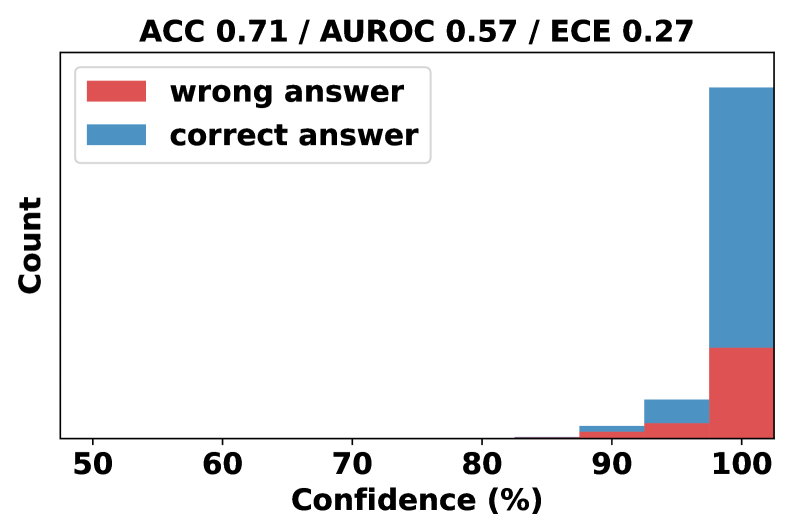<details> <summary>x4.png Details</summary>  ### Visual Description ## Stacked Histogram: Confidence vs. Count for Correct and Wrong Answers ### Overview The image is a stacked histogram showing the distribution of confidence levels for correct and wrong answers. The x-axis represents confidence levels in percentage, and the y-axis represents the count. The histogram is stacked, with the count of wrong answers (red) stacked on top of the count of correct answers (blue) for each confidence interval. The title provides overall performance metrics: ACC (Accuracy) = 0.71, AUROC (Area Under the Receiver Operating Characteristic curve) = 0.57, and ECE (Expected Calibration Error) = 0.27. ### Components/Axes * **Title:** ACC 0.71 / AUROC 0.57 / ECE 0.27 * **X-axis:** Confidence (%) - Ranges from 50 to 100 in increments of 10. * **Y-axis:** Count * **Legend:** Located in the top-left corner. * Red: wrong answer * Blue: correct answer ### Detailed Analysis * **Confidence Levels:** The x-axis is marked at 50, 60, 70, 80, 90, and 100. * **Data Series:** * **Correct Answers (Blue):** The count of correct answers is very low until the 90-100% confidence range, where it increases dramatically. * **Wrong Answers (Red):** The count of wrong answers is very low until the 90-100% confidence range, where it increases. * **Specific Data Points (Approximate):** * **50-60% Confidence:** Both correct and wrong answers have a count of approximately 0. * **60-70% Confidence:** Both correct and wrong answers have a count of approximately 0. * **70-80% Confidence:** Both correct and wrong answers have a count of approximately 0. * **80-90% Confidence:** Both correct and wrong answers have a count of approximately 0. * **90-100% Confidence:** The count of correct answers is significantly higher than the count of wrong answers. The count of correct answers is approximately 15, while the count of wrong answers is approximately 3. ### Key Observations * Most answers, both correct and wrong, are given with high confidence (90-100%). * The number of correct answers with high confidence is much greater than the number of wrong answers with high confidence. * The model rarely provides answers with low confidence (50-90%). ### Interpretation The stacked histogram suggests that the model tends to be more confident in its answers, regardless of whether they are correct or wrong. The high accuracy (ACC = 0.71) indicates that the model is generally correct, but the non-perfect AUROC (0.57) and ECE (0.27) values suggest that the model's confidence is not perfectly calibrated with its actual performance. Specifically, the ECE value of 0.27 indicates that the model is not well-calibrated, meaning that its predicted probabilities do not accurately reflect the true likelihood of correctness. The model is overconfident in some of its predictions. </details> (a) "You are a confident GPT". 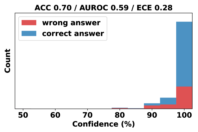<details> <summary>x5.png Details</summary>  ### Visual Description ## Stacked Histogram: Confidence vs. Count of Correct/Wrong Answers ### Overview The image is a stacked histogram showing the distribution of confidence levels for correct and wrong answers. The x-axis represents confidence levels in percentage, and the y-axis represents the count. The histogram is stacked, with the count of wrong answers shown in red and the count of correct answers shown in blue. The title provides the accuracy (ACC), Area Under the Receiver Operating Characteristic Curve (AUROC), and Expected Calibration Error (ECE) values. ### Components/Axes * **Title:** ACC 0.70 / AUROC 0.59 / ECE 0.28 * **X-axis:** Confidence (%) with markers at 50, 60, 70, 80, 90, and 100. * **Y-axis:** Count (no specific numerical markers are provided, only the label). * **Legend:** Located in the top-left corner. * Red: wrong answer * Blue: correct answer ### Detailed Analysis The histogram shows the distribution of confidence levels for correct and wrong answers. * **Confidence 50-60%:** No data present. * **Confidence 60-70%:** No data present. * **Confidence 70-80%:** A very small red bar (wrong answer) is visible. The count is approximately 0-5. * **Confidence 80-90%:** A small red bar (wrong answer) is visible. The count is approximately 0-5. * **Confidence 90-100%:** A red bar (wrong answer) and a blue bar (correct answer) are stacked. The red bar's count is approximately 5-10, and the blue bar's count is approximately 5-10. * **Confidence 100%:** A red bar (wrong answer) and a blue bar (correct answer) are stacked. The red bar's count is approximately 10-15, and the blue bar's count is approximately 40-50. **Trend Verification:** * **Correct Answers (Blue):** The count of correct answers increases significantly as confidence increases, with the highest count at 100% confidence. * **Wrong Answers (Red):** The count of wrong answers is low across all confidence levels, with a slight increase at 100% confidence. ### Key Observations * The vast majority of answers with high confidence (100%) are correct. * There are very few answers with low confidence (below 90%). * The model appears to be well-calibrated, as high confidence generally corresponds to correct answers. * The model has an accuracy of 70%, an AUROC of 0.59, and an ECE of 0.28. ### Interpretation The stacked histogram illustrates the relationship between the model's confidence and the correctness of its answers. The concentration of correct answers at high confidence levels suggests that the model is generally reliable in its predictions. However, the presence of wrong answers at high confidence indicates some degree of overconfidence or miscalibration. The ACC, AUROC, and ECE values provide a quantitative assessment of the model's performance, with the ECE value indicating the calibration error. A lower ECE value generally indicates better calibration. The AUROC value of 0.59 indicates that the model's ability to discriminate between positive and negative classes is slightly better than random guessing. </details> (b) "You are a cautious GPT". Figure 4: Distribution of the verbalized confidence with different specified role descriptions in prompts. The results are derived when adding "You are a confident GPT" (Left) and "You are a cautious GPT" (Right) to the beginning of the Chain of Thought (CoT) prompt (Table 15). All other aspects of the prompts remain identical to the standard CoT format. | Confident | chatgpt-0613 | 0.7103 | 0.2741 | 0.5679 | 0.7398 | 0.3635 | | --- | --- | --- | --- | --- | --- | --- | | Cautious | chatgpt-0613 | 0.6983 | 0.2812 | 0.5946 | 0.7415 | 0.4009 | Table 7: Performance Comparison of Verbalized Confidence Elicitation with two types of prompt: "You are a confident GPT" and "You are a cautious GPT". The difference between these two prompts seems minimal, suggesting that asking LLMs to take on different personae does not significantly affect the performance. B.3 How is the distribution of Vanilla Verbalized Confidence Across Models and Datasets? 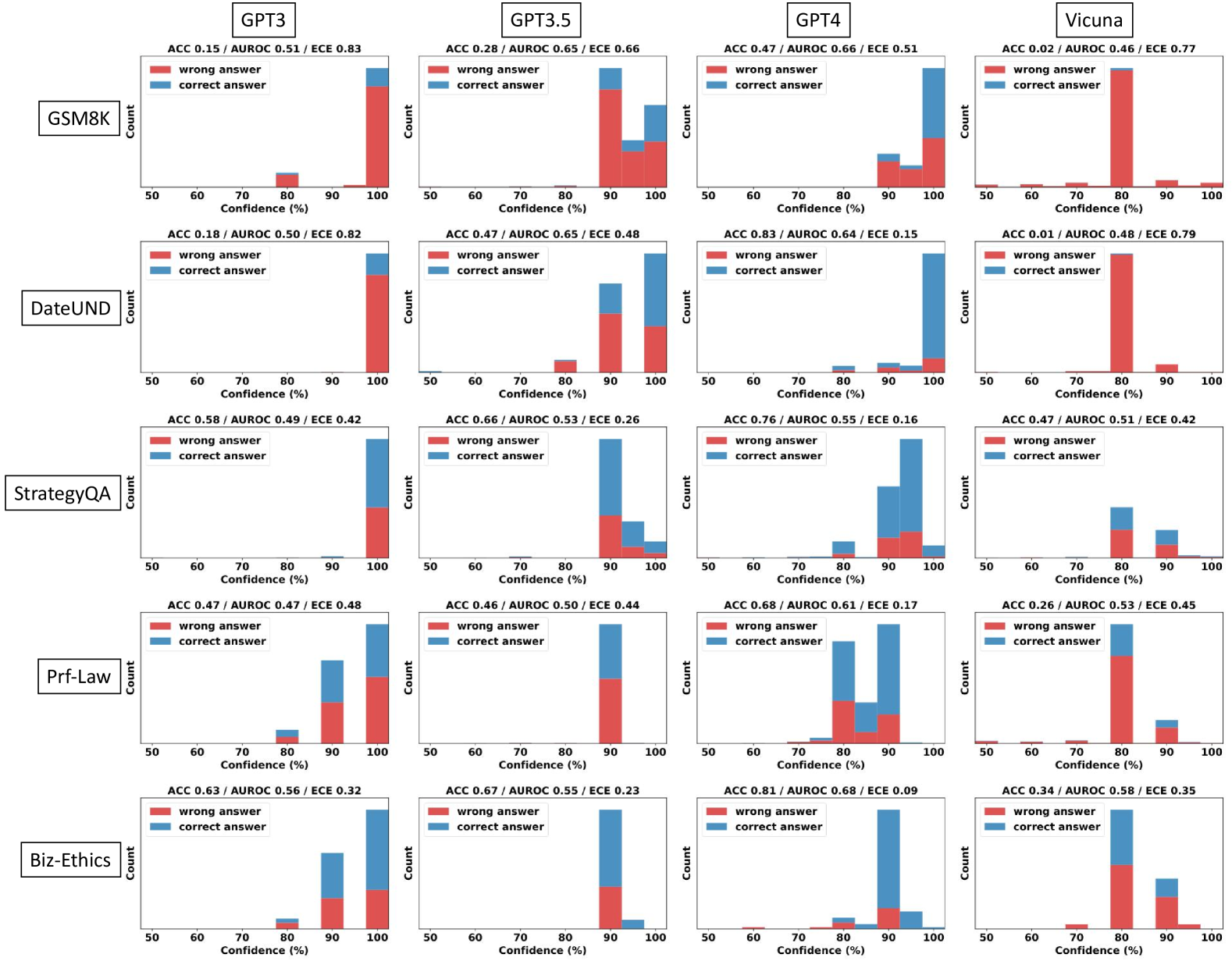<details> <summary>x6.png Details</summary>  ### Visual Description ## Histogram: Model Confidence vs. Accuracy on Various Tasks ### Overview The image presents a series of histograms comparing the confidence levels of four language models (GPT3, GPT3.5, GPT4, and Vicuna) on six different tasks (GSM8K, DateUND, StrategyQA, Prf-Law, and Biz-Ethics). Each histogram shows the distribution of confidence scores for both correct and incorrect answers, allowing for a comparison of model calibration across different tasks and models. ### Components/Axes * **Title:** Model Confidence vs. Accuracy on Various Tasks * **X-axis:** Confidence (%), ranging from 50% to 100% in increments of 10%. * **Y-axis:** Count (frequency of responses within each confidence bin). * **Histograms:** Each subplot represents a combination of a language model and a task. * **Legend:** Located within each subplot: * Red: "wrong answer" * Blue: "correct answer" * **Metrics:** Each subplot includes the following metrics: * ACC: Accuracy * AUROC: Area Under the Receiver Operating Characteristic Curve * ECE: Expected Calibration Error * **Tasks (Y-Axis Labels):** GSM8K, DateUND, StrategyQA, Prf-Law, Biz-Ethics * **Models (X-Axis Labels):** GPT3, GPT3.5, GPT4, Vicuna ### Detailed Analysis **GSM8K** * **GPT3:** ACC 0.15 / AUROC 0.51 / ECE 0.83. The majority of responses, both correct and incorrect, are clustered at 90-100% confidence. The "wrong answer" count is significantly higher than the "correct answer" count at high confidence. * **GPT3.5:** ACC 0.28 / AUROC 0.65 / ECE 0.66. Similar to GPT3, most responses are at 90-100% confidence, with "wrong answers" being more frequent. * **GPT4:** ACC 0.47 / AUROC 0.66 / ECE 0.51. Shows a more balanced distribution, with a noticeable number of "correct answers" at 90-100% confidence, but still dominated by "wrong answers" at high confidence. * **Vicuna:** ACC 0.02 / AUROC 0.46 / ECE 0.77. Almost all responses are clustered at 70-80% confidence, with "wrong answers" dominating. **DateUND** * **GPT3:** ACC 0.18 / AUROC 0.50 / ECE 0.82. High confidence (90-100%) for most answers, with "wrong answers" being more frequent. * **GPT3.5:** ACC 0.47 / AUROC 0.65 / ECE 0.48. High confidence (90-100%) for most answers, with a higher proportion of "correct answers" compared to GPT3. * **GPT4:** ACC 0.83 / AUROC 0.64 / ECE 0.15. Most "correct answers" are at 90-100% confidence. "Wrong answers" are relatively infrequent. * **Vicuna:** ACC 0.01 / AUROC 0.48 / ECE 0.79. Almost all responses are clustered at 70-80% confidence, with "wrong answers" dominating. **StrategyQA** * **GPT3:** ACC 0.58 / AUROC 0.49 / ECE 0.42. Most "correct answers" are at 90-100% confidence. * **GPT3.5:** ACC 0.66 / AUROC 0.53 / ECE 0.26. Most "correct answers" are at 90-100% confidence. * **GPT4:** ACC 0.76 / AUROC 0.55 / ECE 0.16. Most "correct answers" are at 90-100% confidence. * **Vicuna:** ACC 0.47 / AUROC 0.51 / ECE 0.42. A mix of confidence levels, with a peak at 70-80% confidence. **Prf-Law** * **GPT3:** ACC 0.47 / AUROC 0.47 / ECE 0.48. A mix of confidence levels, with a peak at 90-100% confidence. * **GPT3.5:** ACC 0.46 / AUROC 0.50 / ECE 0.44. A mix of confidence levels, with a peak at 90-100% confidence. * **GPT4:** ACC 0.68 / AUROC 0.61 / ECE 0.17. A mix of confidence levels, with a peak at 80-90% confidence. * **Vicuna:** ACC 0.26 / AUROC 0.53 / ECE 0.45. Most "wrong answers" are at 70-80% confidence. **Biz-Ethics** * **GPT3:** ACC 0.63 / AUROC 0.56 / ECE 0.32. Most "correct answers" are at 90-100% confidence. * **GPT3.5:** ACC 0.67 / AUROC 0.55 / ECE 0.23. Most "correct answers" are at 90-100% confidence. * **GPT4:** ACC 0.81 / AUROC 0.68 / ECE 0.09. Most "correct answers" are at 90-100% confidence. * **Vicuna:** ACC 0.34 / AUROC 0.58 / ECE 0.35. A mix of confidence levels, with a peak at 70-80% confidence. ### Key Observations * **Calibration Issues:** GPT3 and GPT3.5 tend to be overconfident, often assigning high confidence to incorrect answers, especially on GSM8K and DateUND. * **GPT4 Improvement:** GPT4 generally shows better calibration, with higher accuracy and lower ECE scores. It tends to assign high confidence more often to correct answers. * **Vicuna's Underconfidence:** Vicuna tends to cluster its responses around 70-80% confidence, regardless of the task or correctness of the answer. This suggests underconfidence. * **Task Difficulty:** GSM8K and DateUND appear to be more challenging tasks, as indicated by the lower accuracy scores across all models. * **AUROC Discrepancies:** The AUROC scores do not always correlate perfectly with accuracy, suggesting that the models' ability to discriminate between correct and incorrect answers varies. ### Interpretation The histograms reveal significant differences in calibration among the four language models. GPT3 and GPT3.5 exhibit overconfidence, particularly on tasks like GSM8K and DateUND, where they frequently assign high confidence to incorrect answers. This suggests that these models are poorly calibrated and may not be reliable for tasks requiring accurate confidence estimation. GPT4 demonstrates improved calibration compared to its predecessors, with higher accuracy and lower ECE scores. This indicates that GPT4 is better at aligning its confidence with its actual performance. Vicuna, on the other hand, appears to be underconfident, clustering its responses around 70-80% confidence regardless of the task or correctness of the answer. This suggests that Vicuna may benefit from calibration techniques to improve its confidence estimation. The task difficulty also plays a role, with GSM8K and DateUND being more challenging than the other tasks. This is reflected in the lower accuracy scores across all models for these tasks. Overall, the histograms provide valuable insights into the calibration of different language models and highlight the importance of evaluating and improving model confidence estimation for reliable decision-making. </details> Figure 5: Empirical distribution of vanilla verbalized confidence across 4 models and 5 datasets. The prompt used is in Table 14. From this figure, we can observe that 1) the confidence levels primarily range between 80% and 100%, often in multiples of 5; 2) a large portion of incorrect predictions (red) has been observed even in the 100% confidence bar, indicating significant overconfidence. Figure 5 presents the empirical distribution of vanilla verbalized confidence across 4 models and 5 datasets. Notably, all the models output confidence as the multiples of 5, with most values ranging between the 80% to 100% range. This behavior resembles the patterns identified in the training corpus for GPT-like models as discussed by Zhou et al. (2023). Such behavior suggests that models might be imitating human expressions when verbalizing confidence. B.4 Detailed Performance of Different Prompting Strategies Multi-step and Top-K prompting strategies demonstrate promising results in reducing ECE and improving AUROC, with Top-K being relatively more effective. Figure 6 presents a comparison of various prompting strategies (CoT, Multi-Step, Top-K) against vanilla verbalized confidence. The detailed performance of CoT, Multi-Step, and Top-K prompt can be found in Table 8, Table 9 and Table 10, respectively. Judging from the ’average’ bar, which computes the mean value across five datasets, both Multi-step and Top-K prompting strategies effectively reduce ECE and enhance AUROC. Moreover, Top-K shows relatively better performance improvements. The intuition behind this improvement is that this prompting strategy, requesting the model to generate multiple guesses along with their corresponding confidences, naturally nudges the model to be aware of the existence of various possible answers, preventing overconfidence in a single response and promoting re-evaluation of given answers. 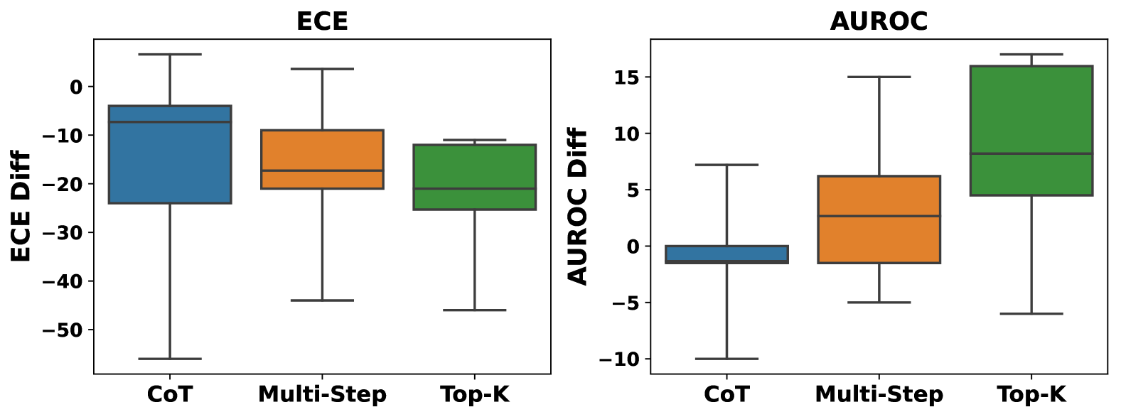<details> <summary>x7.png Details</summary>  ### Visual Description ## Box Plot: ECE Diff and AUROC Diff Comparison ### Overview The image presents two box plots side-by-side, comparing the distributions of "ECE Diff" (Expected Calibration Error Difference) and "AUROC Diff" (Area Under the Receiver Operating Characteristic Curve Difference) across three different methods: "CoT" (Chain-of-Thought), "Multi-Step", and "Top-K". The box plots visually summarize the central tendency, spread, and skewness of the data for each method and metric. ### Components/Axes **Left Plot (ECE):** * **Title:** ECE * **Y-axis:** ECE Diff, with scale markers at 0, -10, -20, -30, -40, and -50. * **X-axis:** Categorical, representing the three methods: CoT, Multi-Step, and Top-K. **Right Plot (AUROC):** * **Title:** AUROC * **Y-axis:** AUROC Diff, with scale markers at -10, -5, 0, 5, 10, and 15. * **X-axis:** Categorical, representing the three methods: CoT, Multi-Step, and Top-K. **Legend (Implicit):** * CoT: Represented by blue boxes. * Multi-Step: Represented by orange boxes. * Top-K: Represented by green boxes. ### Detailed Analysis **Left Plot (ECE Diff):** * **CoT (Blue):** The box extends from approximately -24 to -8. The median is around -14. The upper whisker extends to approximately 2, and the lower whisker extends to approximately -56. * Trend: The ECE Diff for CoT is centered around -14, with a wide spread indicating high variability. * **Multi-Step (Orange):** The box extends from approximately -21 to -12. The median is around -16. The upper whisker extends to approximately 4, and the lower whisker extends to approximately -44. * Trend: The ECE Diff for Multi-Step is centered around -16, with a moderate spread. * **Top-K (Green):** The box extends from approximately -21 to -11. The median is around -16. The upper whisker extends to approximately 2, and the lower whisker extends to approximately -46. * Trend: The ECE Diff for Top-K is centered around -16, with a moderate spread. **Right Plot (AUROC Diff):** * **CoT (Blue):** The box extends from approximately -2 to 0. The median is around -1. The upper whisker extends to approximately 8, and the lower whisker extends to approximately -10. * Trend: The AUROC Diff for CoT is centered around -1, with a moderate spread. * **Multi-Step (Orange):** The box extends from approximately -1 to 4. The median is around 2. The upper whisker extends to approximately 15, and the lower whisker extends to approximately -5. * Trend: The AUROC Diff for Multi-Step is centered around 2, with a wide spread. * **Top-K (Green):** The box extends from approximately 4 to 10. The median is around 8. The upper whisker extends to approximately 17, and the lower whisker extends to approximately -3. * Trend: The AUROC Diff for Top-K is centered around 8, with a wide spread. ### Key Observations * For ECE Diff, all three methods have negative median values, indicating a general tendency to underestimate the calibration error. CoT has the widest spread. * For AUROC Diff, Top-K shows a significantly higher median value compared to CoT and Multi-Step, suggesting better performance in terms of discrimination. ### Interpretation The box plots provide a comparative view of the performance of three different methods (CoT, Multi-Step, and Top-K) based on two metrics: ECE Diff and AUROC Diff. * **ECE Diff:** The negative values across all methods suggest that, on average, these methods tend to underestimate the true calibration error. The wider spread for CoT indicates that its performance is more variable compared to Multi-Step and Top-K. * **AUROC Diff:** Top-K stands out with a higher median AUROC Diff, implying that it generally provides better discrimination compared to the other two methods. The spread of the data suggests that the performance of Multi-Step and Top-K can vary significantly. In summary, while all methods show a tendency to underestimate calibration error, Top-K appears to offer better discrimination performance based on the AUROC metric. The variability in performance, as indicated by the spread of the box plots, should also be considered when selecting a method for a specific application. </details> Figure 6: Performance Comparison of four verbalized confidence methods: vanilla, CoT, Multi-Step, Top-K in terms of ECE and AUROC for five types of datasets on GPT-3.5. Refer to Table 10 for detailed results. Table 8: Improvement of verbalized confidence with Chain-of-Thought Prompts | GSM8K | ✗ | 28 | 66 | 65 | | --- | --- | --- | --- | --- | | ✓ | 80.3 | 10 | 55 | | | DateUnd | ✗ | 47 | 48 | 65 | | ✓ | 73.2 | 23 | 57 | | | StrategyQA | ✗ | 65.8 | 26 | 53 | | ✓ | 67.9 | 22 | 60 | | | Prf-Law | ✗ | 45.5 | 44 | 50 | | ✓ | 51.7 | 37 | 49 | | | Biz-Ethics | ✗ | 67 | 23 | 55 | | ✓ | 61 | 30 | 56 | | Table 9: Evaluation of multistep verbalized confidence for GPT-3.5 Models | GSM8K | ✗ | 80.3 | 10 | 55 | | --- | --- | --- | --- | --- | | ✓ | 76.2 | 22 | 60 | | | DateUnd | ✗ | 73.2 | 23 | 57 | | ✓ | 63.6 | 26 | 72 | | | StrategyQA | ✗ | 67.9 | 22 | 60 | | ✓ | 68.7 | 17 | 59 | | | Prf-Law | ✗ | 51.7 | 37 | 49 | | ✓ | 49.6 | 27 | 49 | | | Biz-Ethics | ✗ | 61 | 30 | 56 | | ✓ | 61.6 | 27 | 60 | | B.5 Top-K Verbalized Confidence Performance The detailed experiments performance of Top-K verbalized confidence can be found in Table 10. Table 10: Evaluation of Top-K verbalized confidence on GPT-3.5. | Dataset | GPT3.5 | | | | --- | --- | --- | --- | | ACC(%) | ECE | AUROC | | | GSM8K | 22.8 | 19.6 | 58.5 | | DateUnd | 33.3 | 26.1 | 74.2 | | StrategyQA | 61.3 | 14 | 61.3 | | Prf-Law | 42.2 | 16.7 | 58.9 | | Biz-Ethics | 67.0 | 12.4 | 73.3 | B.6 Impact of Misleading Prompts in Misleading Sampling Strategy To study the effect of different misleading prompts used in misleading sampling strategy, we categorize the prompts into three types: Weak Claim, Strong Claim, and External Source. The specific prompts are shown in Table 11. The Weak Claim category represents prompts that exhibit uncertainty, such as "I vaguely remember the answer is" or "I think the answer should be". These prompts suggest that the user is providing misleading information to the Large Language Model (LLM) but lacks confidence in the information provided. The Strong Claim category includes prompts like "I am pretty sure that this is" or "I am very confident that", which express a high degree of certainty. The External Source category represents prompts that cite external sources as their evidence, such as "Wikipedia says" or "the latest research shows that". Our experimental results (Table 11) indicate that the Weak Claim category performs better. A possible explanation is that on one hand even providing weak misleading information, the model will analyze and reassess their answers. On the other hand, since the misleading answers are generated randomly, confidently providing this information can sometimes lead to negative effects. For example, the model provides a correct answer with moderate confidence. However, if a misleading hint is provided with high confidence or is supported by an external source, the model may be inclined to believe the prompt and alter its predictions. Table 11: Different Prompts used for misleading sampling strategy. | Weak Claim | Hint: I think the answer should be | | --- | --- | | Weak Claim | Hint: I read online the answer is | | Weak Claim | Hint: I vaguely remember the answer is | | Externel Source | Hint: My teacher tells me the answer is | | Externel Source | Hint: The textbook shows that answer is | | Externel Source | Hint: An expert says that the answer is | | Externel Source | Hint: Latest research shows that the answer is | | Externel Source | Hint: Wikipedia claims that the answer is | | Strong Claim | Hint: I am 80% sure the answer is | | Strong Claim | Hint: I am pretty sure the answer is | | Strong Claim | Hint: Undoubtedly the answer is | | Strong Claim | Hint: With my 100% confidence the answer is | Table 12: The performance of varying prompt groups in StrategyQA on GPT-3.5. The group exhibiting the optimal performance is emphasized in bold. The experimental results indicate that the Weak Claim category performs better. | Induced Consistency Confidence | Weak Claim | 19.7 | 62.0 | | --- | --- | --- | --- | | Strong Claim | 19.5 | 61.4 | | | External Source | 18.2 | 60.8 | | | verbalized-consistency confidence | Weak Claim | 19.8 | 65.4 | | Strong Claim | 19.5 | 64.6 | | | External Source | 18.2 | 63.4 | | B.7 Impact of the Number of Candidate Answers We investigate the impact of the number of candidate answers, denoted as $K$ , utilized in the sampling strategy. Specifically, $K$ represents the number of queries used to construct the set of candidate answers for consistency calculation. We illustrate its calibration performance (ECE) and failure prediction performance (AUROC) in relation to varying numbers of $K$ (ranging from $K=1$ to $K=13$ ) in Figure 7. The results indicate that, in terms of AUROC, a higher candidate set size $K$ contributes to superior performance and reduced variance. However, the optimal candidate size $K$ for ECE varies across different datasets. For instance, the StrategyQA dataset exhibits improved performance with a larger $K$ , whereas the Business Ethics dataset generally performs better with a moderate number of candidate answers (e.g., $K=4$ ). This observation can be attributed to the limited variability of misleading information (restricted to 4 types) used in our experiments for the Business Ethics dataset, implying that the introduction of a large number of more queries does not significantly enhance the information pool. Therefore, to strike a balance between computational efficiency and performance, we set the candidate set to be 4 in our study. 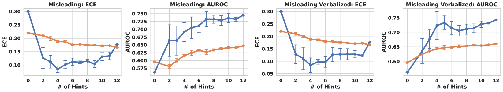<details> <summary>x8.png Details</summary>  ### Visual Description ## Line Charts: Misleading Hints vs. Performance Metrics ### Overview The image contains four line charts, arranged in a 2x2 grid. Each chart plots the relationship between the number of misleading hints (x-axis) and either Expected Calibration Error (ECE) or Area Under the Receiver Operating Characteristic Curve (AUROC) (y-axis). The charts are titled "Misleading: ECE", "Misleading: AUROC", "Misleading Verbalized: ECE", and "Misleading Verbalized: AUROC". Each chart contains two data series, represented by a blue line and an orange line. Error bars are present on the blue lines. ### Components/Axes * **X-axis (all charts):** "# of Hints". Scale ranges from 0 to 12 in increments of 2. * **Y-axis (Misleading: ECE and Misleading Verbalized: ECE):** "ECE". Scale ranges from 0.05 to 0.30 in increments of 0.05. * **Y-axis (Misleading: AUROC and Misleading Verbalized: AUROC):** "AUROC". Scale ranges from 0.575 to 0.750 in increments of 0.025. * **Data Series:** * Blue line: The specific meaning of this line is not explicitly stated in the image. * Orange line: The specific meaning of this line is not explicitly stated in the image. ### Detailed Analysis **1. Misleading: ECE** * **Blue Line Trend:** The blue line starts at approximately 0.30 and decreases sharply until x=4, reaching a value of approximately 0.08. It then increases slightly to approximately 0.12 at x=6, remains relatively flat until x=10, and then increases again to approximately 0.14 at x=12. * Data Points: (0, 0.30), (2, 0.15), (4, 0.08), (6, 0.12), (8, 0.10), (10, 0.11), (12, 0.14) * **Orange Line Trend:** The orange line starts at approximately 0.22 and gradually decreases to approximately 0.17 at x=12. * Data Points: (0, 0.22), (2, 0.21), (4, 0.19), (6, 0.18), (8, 0.18), (10, 0.175), (12, 0.17) **2. Misleading: AUROC** * **Blue Line Trend:** The blue line starts at approximately 0.57 and increases steadily until x=12, reaching a value of approximately 0.75. The rate of increase slows down after x=8. * Data Points: (0, 0.57), (2, 0.66), (4, 0.68), (6, 0.72), (8, 0.73), (10, 0.72), (12, 0.75) * **Orange Line Trend:** The orange line starts at approximately 0.59 and increases gradually to approximately 0.67 at x=12. * Data Points: (0, 0.59), (2, 0.61), (4, 0.63), (6, 0.64), (8, 0.65), (10, 0.66), (12, 0.67) **3. Misleading Verbalized: ECE** * **Blue Line Trend:** The blue line starts at approximately 0.30 and decreases sharply until x=4, reaching a value of approximately 0.08. It then increases slightly to approximately 0.10 at x=6, remains relatively flat until x=10, and then increases again to approximately 0.12 at x=12. * Data Points: (0, 0.30), (2, 0.13), (4, 0.08), (6, 0.10), (8, 0.095), (10, 0.11), (12, 0.12) * **Orange Line Trend:** The orange line starts at approximately 0.22 and gradually decreases to approximately 0.17 at x=12. * Data Points: (0, 0.22), (2, 0.21), (4, 0.19), (6, 0.18), (8, 0.18), (10, 0.17), (12, 0.17) **4. Misleading Verbalized: AUROC** * **Blue Line Trend:** The blue line starts at approximately 0.53 and increases steadily until x=12, reaching a value of approximately 0.76. The rate of increase slows down after x=8. * Data Points: (0, 0.53), (2, 0.64), (4, 0.70), (6, 0.72), (8, 0.71), (10, 0.72), (12, 0.76) * **Orange Line Trend:** The orange line starts at approximately 0.59 and increases gradually to approximately 0.67 at x=12. * Data Points: (0, 0.59), (2, 0.61), (4, 0.63), (6, 0.64), (8, 0.65), (10, 0.66), (12, 0.67) ### Key Observations * For both "Misleading" and "Misleading Verbalized" conditions, the ECE (blue line) initially decreases sharply with the number of hints, then plateaus and slightly increases. The orange line decreases gradually. * For both "Misleading" and "Misleading Verbalized" conditions, the AUROC (blue line) increases steadily with the number of hints. The orange line increases gradually. * The error bars on the blue lines indicate the variability in the data. ### Interpretation The charts suggest that providing misleading hints initially improves the calibration (decreases ECE) and increases the discriminative power (increases AUROC) of a model (blue line). However, after a certain number of hints, the ECE starts to increase again, indicating that too many misleading hints can negatively impact calibration. The AUROC continues to increase, but at a slower rate. The orange line represents a different condition or model, and its performance is less affected by the number of misleading hints. The "Verbalized" condition seems to have a similar effect as the "Misleading" condition, but the initial impact on AUROC is more pronounced. Without knowing what the blue and orange lines represent, it is difficult to draw more specific conclusions. </details> Figure 7: Impact of the number of responses responses on GPT-3.5. The sampling strategy is fixed as misleading. For every given number of misleading hints, we randomly sample the specified number of queries for 5 times and calculate the mean ECE and AUROC, and compute its variance(plotted as error bar). Note that the number of hints plus 1 is the number of responses sampled during experiment. B.8 Performance of different confidence elicitation methods Appendix C Related Works Confidence Elicitation in LLMs. Confidence elicitation refers to the process of estimating LLM’s confidence in their responses, without relying on model fine-tuning or accessing the proprietary information of LLMs. Within this scope, Lin et al. (2022) proposes the concept of verbalized confidence that elicits the model to output confidence directly. However, the evaluation is tailored for pretrained language models that are fine-tuned on specific datasets, and its zero-shot verbalized confidence remains unexplored. Mielke et al. (2022) proposes to train an external calibrator while relies on model representations that are not readily accessible. Zhou et al. (2023) examine the impact of confidence in prompts but does not directly provide confidence to users. Our work aligns most closely with the concurrent study by Tian et al. (2023), which also focuses on the use of prompting strategies. However, our approach diverges by aiming to explore a broader method space, introducing a unified framework consisting of three components and conducting a systematic evaluation of strategies within each. The Top-K method, as proposed in (Tian et al., 2023), serves as an instance within our framework, and its performance can be augmented when integrated with other strategies from our framework. Furthermore, our investigation extends beyond the RLHF-LMs primarily analyzed in the concurrent study, and encompasses a broader spectrum of models. This allows us to probe the implications of different model sizes and structures. Our findings also underscore that all existing methods still face challenges with more complex tasks, contributing to a more holistic understanding of confidence elicitation in the field. Calibration. Modern neural networks are shown to be poorly calibrated, often manifesting overconfidence (Guo et al., 2017; Minderer et al., 2021; Xiong et al., 2023). Calibration seeks to address the issue by aligning the model’s confidence with the accuracy of samples within the same confidence level (Guo et al., 2017; Minderer et al., 2021). To achieve this, a variety of methods have been proposed, which can be broadly divided into scaling-based methods (Guo et al., 2017; Deng et al., 2023; Zhang et al., 2020) and binning-based methods (Zadrozny & Elkan, 2001; Zhang et al., 2020). Within the scope of LLMs, Jiang et al. (2021) investigates the calibration of generative language models (T5, BART, and GPT-2) and discovers that these models’ probabilities on question-answering tasks are poorly calibrated. Similarly, Chen et al. (2022) finds that PLMs are not well calibrated and pretraining improves model calibration. On the other hand, Kadavath et al. (2022) studies the calibration of LLMs (parameter size ranging 800M to 50B), finding that larger models appear to be well-calibrated on multiple choice and true/false questions when provided in the right format. However, these evaluations mainly focus on the probabilities derived from logits, which are unavailable for closed-source LLMs like GPT-4. This also motivates us to study confidence elicitation methods that do not require model fine-tuning or access to model logits or embeddings. Table 13: Performance of different confidence elicitation methods: verbalize-based (Top-K and CoT Verbalized Confidence), consistency-based (Self-Consistency and Induced consistency), and their hybrid combinations. The best-performing method for each dataset is highlighted in bold. | ECE $\downarrow$ | Top-K (M=1) | 39.8 | 40.1 | 14.0 | 16.7 | 12.4 | 24.6 | | --- | --- | --- | --- | --- | --- | --- | --- | | CoT (M=1) | 10.1 | 23.4 | 22.0 | 39.7 | 30.0 | 25.0 | | | Self-Random+Consistency (M=5) | 6.28 | 17.0 | 23.3 | 26.0 | 20.7 | 18.7 | | | Misleading + Cons (M=5) | 8.03 | 20.5 | 21.8 | 18.3 | 17.8 | 17.3 | | | Self-Random + Avg-Conf (M=5) | 9.28 | 14.6 | 15.9 | 18.3 | 15.8 | 14.8 | | | Misleading + Avg-Conf (M=5) | 7.40 | 17.6 | 15.0 | 12.8 | 18.2 | 14.2 | | | ROC $\uparrow$ | Top-K (M=1) | 59.9 | 76.3 | 61.3 | 58.9 | 73.3 | 65.9 | | CoT (M=1) | 54.8 | 57.4 | 59.8 | 52.2 | 56.0 | 56.4 | | | Self-Random+Consistency (M=5) | 92.7 | 66.8 | 60.8 | 65.6 | 79.0 | 73.0 | | | Misleading + Cons (M=5) | 88.6 | 67.3 | 61.5 | 59.3 | 71.3 | 69.6 | | | Self-Random + Avg-Conf (M=5) | 92.5 | 68.8 | 66.2 | 65.3 | 79.5 | 74.5 | | | Misleading + Avg-Conf (M=5) | 88.8 | 63.8 | 65.6 | 60.4 | 72.4 | 70.2 | | | PR-P $\uparrow$ | Top-K (M=1) | 27.7 | 62.8 | 68.4 | 49.3 | 82.2 | 58.1 | | CoT (M=1) | 81.8 | 76.6 | 72.8 | 49.2 | 64.3 | 68.9 | | | Self-Random+Consistency (M=5) | 96.9 | 81.0 | 73.7 | 59.4 | 82.3 | 78.7 | | | Misleading + Cons (M=5) | 95.1 | 81.0 | 74.1 | 54.7 | 77.6 | 76.5 | | | Self-Random + Avg-Conf (M=5) | 97.0 | 84.4 | 78.3 | 60.3 | 83.1 | 80.6 | | | Misleading + Avg-Conf (M=5) | 95.3 | 79.0 | 79.1 | 56.4 | 80.9 | 78.1 | | | PR-N $\uparrow$ | Top-K (M=1) | 80.2 | 79.8 | 45.7 | 56.0 | 50.7 | 62.5 | | CoT (M=1) | 23.1 | 30.7 | 40.5 | 53.9 | 43.7 | 38.4 | | | Self-Random+Consistency (M=5) | 79.7 | 44.6 | 39.5 | 63.8 | 63.4 | 58.2 | | | Misleading + Cons (M=5) | 71.2 | 44.2 | 41.3 | 58.7 | 55.1 | 54.1 | | | Self-Random + Avg-Conf (M=5) | 81.5 | 51.8 | 45.8 | 65.3 | 64.9 | 61.9 | | | Misleading + Avg-Conf (M=5) | 73.5 | 42.4 | 45.4 | 60.9 | 57.1 | 55.9 | | Appendix D Best Practice and Recommendations For Practitioners D.1 What is the recommendation for practitioners? Balancing between efficiency, simplicity, and effectiveness, we recommend a stable-performing method from our empirical results as advice for practitioners: Top-K prompt + Self-Random sampling + Avg-Conf or Pair-Rank aggregation. The recommendation is based on: 1) Top-K outperforms all other methods on GPT-3.5 and is comparable to the top-performing method Self-Probing on GPT4. Compared to Self-Probing which requires two inference phases, the Top-K prompt is chosen for the balance between effectiveness and efficiency. 1) As shown in Sec 5.3, ensemble methods (e.g., $M=5$ ) are consistently more effective than verbalized confidence ( $M=1$ ) in eliciting a model’s confidence. Regarding the sampling strategies, Self-Random is selected for being more straightforward and commonly used, since the performance difference of different sampling strategies is minimal.. 3) For aggregation, strategies based on both answers and verbalized confidences (e.g., Avg-Conf and Pair-Rank) outperform *aggregation based on answers only (e.g., consistency)*. Then we recommend Pair-Rank and Avg-Conf for different downstream tasks according to their relatively good performance on different metrics. For example, for tasks that prioritize the exact confidence values, like calculating expected risk, Pair-Rank is recommended, while Avg-Conf is better suited for tasks related to failure prediction, e.g., factual error detection. Additionally, it is noteworthy that using Top-K alone does not improve accuracy as much as Chain of Thought (CoT), but the use of ensemble methods compensates for this. D.2 What are the considerations when using black-box confidence elicitation algorithms? Careful consideration is necessary due to significant limitations: 1) The reliability of the given confidence must be assessed by considering multiple metrics, such as both ECE and AUROC. As discussed in section 5.2, a high ECE does not imply that the model’s outputs accurately represent model correctness. Metrics including AUROC and detailed information such as the confidence distribution plot should also be considered for a comprehensive evaluation and better understanding. 2) LLMs are not explicitly modeled to express uncertainty in textual outputs, and descriptions of uncertainty in the training corpus are mostly human expressions, which are often considered inaccurate (Garthwaite et al., 2005b). Dependence on such confidence for real-world applications requires careful checking, especially given the consistently high confidence levels shown in Figure 2, no matter whether the question is correctly answered or not. D.3 Discussions on why some strategies work, and why some do not work In this section, we discuss the effective strategies and analyze the rationale behind these mechanisms. Sampling Consistency among multiple responses is more effective compared to verbalized confidence ( $M=1$ ), with particularly notable improvements on the arithmetic task. This is because sampling more queries allows us to directly approximate the model’s internal distribution, $P_{model}(\mathbf{x}_{t}|\mathbf{x}_{1:t-1})$ , which is trained to mirror the ground truth data distribution. Issues making this method ineffective can be: 1) the model’s poor calibration (Kuhn et al., 2023), i.e., $P_{model}(\mathbf{x}_{t}|\mathbf{x}_{1:t-1})$ does not align well with $P_{data}(\mathbf{x}_{t}|\mathbf{x}_{1:t-1})$ ; or 2) the computational constraints limiting the number of sampled queries, leading to inaccurate estimates. Aggregation Aggregation based on answers and verbalized confidences (e.g., Avg-Conf and Pair-Rank) outperforms aggregation based on answers only (e.g., consistency), especially when LLM queries are costly and the number of queries we can sample is constrained. This is due to the coarse granularity of the consistency-based aggregation’s output—limited to 6 possible values (0, 0.2, 0.4, 0.6, 0.8, 1) when M=5. This can lead to poor calibration performance. The verbalized confidence, despite being less precise, still captures the model’s uncertainty tendency and allows for finer-grained output values, and hence can be combined to enhance calibration performance. Verbalized Confidence For verbalized confidence, we note that humans are able to verbalize their uncertainty, e.g., giving insight as to whether our answers and reasonings are correct or not. So it is reasonable to expect LLMs to have also learned this ability, or to learn it at some point in the future. The current suboptimal performance of verbalized confidence points to an important research gap, and this might be explained by the inherent inaccuracy of the training data, particularly human expressions of uncertainty. For example, as studied by Garthwaite et al. (2005a), humans sometimes tend to exaggerate their a priori probability for an event that has occurred. Prompting Strategy In addition, compared to Vanilla prompt, Top-K, CoT, and Multi-Step can significantly reduce ECE in ChatGPT. We argue that the improvement is largely due to these prompt strategies enhancing the model’s accuracy, which narrows the gap between average confidence and actual accuracy, rather than a significant boost in their ability to differentiate between correct and incorrect samples. This is also supported by the modest gains in AUROC and AUPRC, compared to the significant improvement in ECE. Appendix E Experiment Setup E.1 Datasets To evaluate the quality of confidence estimates in varied tasks, we select the tasks of commonsense reasoning, arithmetic calculation, symbolic reasoning, professional knowledge, and ethical knowledge as evaluation benchmarks. In detail, the datasets for each task are listed below: - Commonsense Reasoning: Sports Understanding (SportUND) dataset (Kim, 2021) and StrategyQA dataset (Geva et al., 2021) from BigBench (Ghazal et al., 2013). We select StrategyQA as the more representative dataset since it contains more data. - Arithmetic Reasoning: Graduate School Math (GSM8K) dataset (Cobbe et al., 2021) and Simple Variations on Arithmetic Math word Problems (SVAMP) dataset (Patel et al., 2021). We select GSM9K as the more representative dataset because it has a wider usage. - Symbolic Reasoning: Date Understanding (DateUnd) dataset (Wu & Wang, 2021) and Object Counting (ObjectCou) dataset (Wang et al., 2019) in BigBench. We select Date Understanding as the more representative dataset since it is more difficult than Object Counting. - Professional Knowledge: Professional Law (Prf-Law) dataset from MMLU (Massive Multitask Language Understanding) (Hendrycks et al., 2021) - Ethical Knowledge: business ethics (Biz-Ethics) dataset from MMLU (Hendrycks et al., 2021). E.2 Evaluation Metrics In line with previous evaluation setting in (Naeini et al., 2015; Yuan et al., 2021; Xiong et al., 2022), we use confidence calibration and failure prediction metrics to measure estimated confidence: - Expected Calibration Error (ECE): It measures the calibration of a classifier by quantifying the discrepancy between predicted probabilities and observed accuracy. - Area Under the Receiver Operating Characteristic curve (AUROC): It assesses the discriminative ability of a classifier across different classification thresholds (Boyd et al., 2013). - Area under the Precision-Recall Curve (AUPRC): It measures the trade-off between precision and recall at different classification thresholds. Specifically, AUPRC-Positive measures the AUPRC for positive instances and AUPRC-Negative is for negative samples. Specifically, calibration metrics (ECE) measure the alignment of confidence scores with the ground truth uncertainty, enabling their utilization in tasks such as risk assessment; while failure detection (AUROC and AUPOR) metrics measure whether the confidence score can appropriately differentiate correct answers and incorrect answers. These metrics also play a crucial role in accurately assessing calibration measurements in works such as Mielke et al. (2022) and Solano et al. (2021) . E.3 Models In our experiments, we incorporate a range of representative LLMs of different scales, including Vicuna (Chiang et al., 2023), GPT3 (Brown et al., 2020), GPT3.5 (GPT3.5) (OpenAI, 2021), and GPT4 (OpenAI, 2023). The number of parameters in each model is 13 billion for Vicuna, 175 billion for GPT3, and larger for GPT3.5 and GPT4. While GPT3.5 and GPT4 have been widely acknowledged due to their outstanding performances, GPT3 is selected as a former version of them. Vicuna is a smaller model fine-tuned from LLaMA (Touvron et al., 2023a). 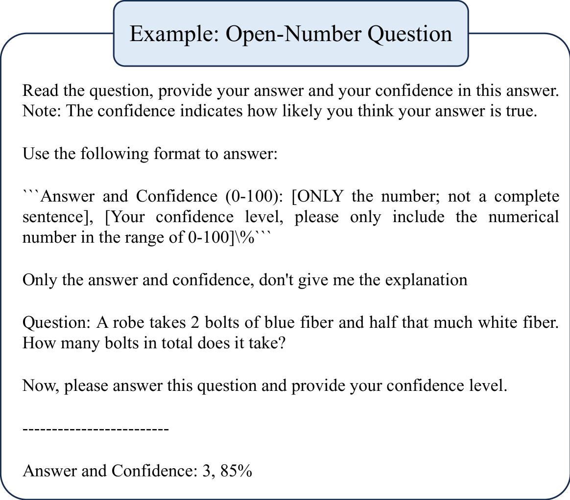<details> <summary>x9.png Details</summary>  ### Visual Description ## Instructional Document: Open-Number Question Example ### Overview This image presents an example of an "Open-Number Question." It provides instructions on how to answer such a question, emphasizing the format for providing both the answer and a confidence level. It includes a sample question and an example response. ### Components/Axes * **Title:** Located at the top in a blue rounded-corner box: "Example: Open-Number Question" * **Instructions:** A block of text providing guidance on how to answer the question and the required format. * **Question:** A sample question about calculating the total bolts of fiber. * **Answer Space:** A blank space is provided for the answer. * **Example Answer:** An example of how to provide the answer and confidence level. ### Detailed Analysis * **Title Text:** The title "Example: Open-Number Question" is contained within a light blue box with rounded corners located in the upper center of the image. * **Instruction Text:** The instructions section contains the following information: * "Read the question, provide your answer and your confidence in this answer." * "Note: The confidence indicates how likely you think your answer is true." * "Use the following format to answer:" * "```Answer and Confidence (0-100): [ONLY the number; not a complete sentence], [Your confidence level, please only include the numerical number in the range of 0-100]\%```" * "Only the answer and confidence, don't give me the explanation" * **Sample Question:** "Question: A robe takes 2 bolts of blue fiber and half that much white fiber. How many bolts in total does it take?" * **Answer Space:** A series of underscores, "-------------" is provided after the question, as a place to write the answer. * **Example Answer:** "Answer and Confidence: 3, 85%" ### Key Observations * The instructions emphasize providing only the numerical answer and confidence level without explanation. * The confidence level is specified to be a number between 0 and 100, followed by a percentage sign. * The sample question requires a simple calculation: 2 bolts of blue fiber + 1 bolt of white fiber (half of 2) = 3 bolts in total. * The example answer of "3, 85%" correctly answers the question and provides a confidence level. ### Interpretation The image provides a clear example of how to answer open-number questions, particularly focusing on eliciting the respondent's confidence in their answer. The structure emphasizes succinctness and quantification of uncertainty, likely for subsequent analysis of response accuracy and confidence calibration. The example is designed to guide respondents in adhering to the specified format, ensuring consistency in data collection. </details> Figure 8: Example of a complete prompt and the model’s output. The vanilla prompt is used. E.4 Implementation Details For the use of sampling strategy, we sample $M=5$ responses. For the use of Self-Random, we set the temperature hyper-parameter as 0.7 to gather a more diverse answer set, as suggested in Wang et al. (2022). The p Appendix F Prompts The prompts used in our work consist of three components: the description, the question, and the misleading hints (used for misleading sampling strategy). The description part outlines the definition of the task presented to the LLMs, requesting them to provide an answer together with the confidence level for the answer. See Figure 8 for a complete example of full prompt and the model’s output. The detailed prompt is provided below: 1. Vanilla: Table 14 1. Chain-of-Thought-based: Table 15 1. Self-Probing: Table 16 1. Multi-Step: Table 17 1. Top-K: Table 18 Table 14: The designed vanilla prompt for two different tasks. | Multi-choice questions Open-number questions | Read the question, provide your answer and your confidence in this answer. Note: The confidence indicates how likely you think your answer is true. Use the following format to answer: “‘Answer and Confidence (0-100): [ONLY the option letter; not a complete sentence], [Your confidence level, please only include the numerical number in the range of 0-100]%”’ Only the answer and confidence, don’t give me the explanation. Question:[Specific Question Here] Now, please answer this question and provide your confidence level. Read the question, provide your answer and your confidence in this answer. Note: The confidence indicates how likely you think your answer is true. Use the following format to answer: “‘Answer and Confidence (0-100): [ONLY the number; not a complete sentence], [Your confidence level, please only include the numerical number in the range of 0-100]%”’ Only the answer and confidence, don’t give me the explanation. Question:[Specific Question Here] Now, please answer this question and provide your confidence level. | | --- | --- | Table 15: The prompt designed for Chain-of-Thought prompting strategy. | Multi-choice questions Open-number questions | Read the question, analyze step by step, provide your answer and your confidence in this answer. Note: The confidence indicates how likely you think your answer is true. Use the following format to answer: “‘Explanation: [insert step-by-step analysis here] Answer and Confidence (0-100): [ONLY the option letter; not a complete sentence], [Your confidence level, please only include the numerical number in the range of 0-100]%”’ Only give me the reply according to this format, don’t give me any other words. Question:[Specific Question Here] Now, please answer this question and provide your confidence level. Let’s think it step by step. Read the question, analyze step by step, provide your answer and your confidence in this answer. Note: The confidence indicates how likely you think your answer is true. Use the following format to answer: “‘Explanation: [insert step-by-step analysis here] Answer and Confidence (0-100): [ONLY the number; not a complete sentence], [Your confidence level, please only include the numerical number in the range of 0-100]%”’ Only give me the reply according to this format, don’t give me any other words. Question:[Specific Question Here] Now, please answer this question and provide your confidence level. Let’s think it step by step. | | --- | --- | Table 16: The prompt designed for self-probing prompting strategy. | The prompt designed for self-probing prompting strategy | | --- | | Question: [The specific question] Possible Answer: [The answer candidates] Q: How likely is the above answer to be correct? Please first show your reasoning concisely and then answer with the following format: “‘Confidence: [the probability of answer {answer} to be correct, not the one you think correct, please only include the numerical number]”’ | Table 17: The designed prompt for multi-step prompting strategy. | Question | Read the question, break down the problem into K steps, think step by step, give your confidence in each step, and then derive your final answer and your confidence in this answer. Note: The confidence indicates how likely you think your answer is true. Use the following format to answer: “‘Step 1: [Your reasoning], Confidence: [ONLY the confidence value that this step is correct]% … Step K: [Your reasoning], Confidence: [ONLY the confidence value that this step is correct]% Final Answer and Overall Confidence (0-100): [ONLY the answer type; not a complete sentence], [Your confidence value]%”’ | | --- | --- | Table 18: Prompts used to elicit Top-K Verbalized Confidence. | Question | Provide your k best guesses and the probability that each is correct (0% to 100%) for the following question. Give ONLY the task output description of your guesses and probabilities, no other words or explanation. For example: G1: <ONLY the task output description of first most likely guess; not a complete sentence, just the guess!> P1: <ONLY the probability that G1 is correct, without any extra commentary whatsoever; just the probability!> … Gk: <ONLY the task output description of k-th most likely guess> Pk: <ONLY the probability that Gk is correct, without any extra commentary whatsoever; just the probability!> | | --- | --- |