# Perceptual Quality Enhancement of Sound Field Synthesis Based on Combination of Pressure and Amplitude Matching
**Authors**: Keisuke Kimura, Shoichi Koyama, Hiroshi Saruwatari
## PERCEPTUAL QUALITY ENHANCEMENT OF SOUND FIELD SYNTHESIS BASED ON COMBINATION OF PRESSURE AND AMPLITUDE MATCHING
Keisuke Kimura, 1 Shoichi Koyama, 2 Hiroshi Saruwatari 1
1 The University of Tokyo, 7-3-1 Hongo, Bunkyo-ku, Tokyo 113-8656, Japan 2 National Institute of Informatics, 2-1-2 Hitotsubashi, Chiyoda-ku, Tokyo 101-8430, Japan koyama.shoichi@ieee.org
## ABSTRACT
Asound field synthesis method enhancing perceptual quality is proposed. Sound field synthesis using multiple loudspeakers enables spatial audio reproduction with a broad listening area; however, synthesis errors at high frequencies called spatial aliasing artifacts are unavoidable. To minimize these artifacts, we propose a method based on the combination of pressure and amplitude matching. On the basis of the human's auditory properties, synthesizing the amplitude distribution will be sufficient for horizontal sound localization. Furthermore, a flat amplitude response should be synthesized as much as possible to avoid coloration. Therefore, we apply amplitude matching, which is a method to synthesize the desired amplitude distribution with arbitrary phase distribution, for high frequencies and conventional pressure matching for low frequencies. Experimental results of numerical simulations and listening tests using a practical system indicated that the perceptual quality of the sound field synthesized by the proposed method was improved from that synthesized by pressure matching.
Index Terms -sound field synthesis, sound field reproduction, pressure matching, amplitude matching, spatial audio
## 1. INTRODUCTION
Sound field synthesis/reproduction is a technique to recreate a spatial sound using multiple loudspeakers (or secondary sources). One of its prospective applications is spatial audio for virtual/augmented reality, which enables spatial audio reproduction with a broader listening area than in the case of conventional spatial audio techniques, such as multichannel surround sound and binaural synthesis.
Sound field synthesis methods based on the minimization of the squared error between synthesized and desired sound fields, such as pressure matching and mode matching [1-6], have practical advantages compared with methods based on analytical representations derived from boundary integral equations such as wave field synthesis and higher-order ambisonics [4,7-13], since the array geometry of the secondary sources can be arbitrary. In particular, pressure matching is widely used because of its simple implementation.
Awell-known issue of the sound field synthesis methods is spatial aliasing artifacts . That is, depending on the secondary source placement, the synthesis accuracy can significantly decrease at high frequencies, which can lead to the degradation of sound localization for listeners and distortion of timbre, or coloration , of source signals. Thus, the perceptual quality of the synthesized sound field can considerably deteriorate.
To improve the perceptual quality, we propose a method combining amplitude matching , which was originally proposed for mul- tizone sound field control [14, 15], with pressure matching. Amplitude matching is a method to synthesize the desired amplitude (or magnitude) distribution, leaving the phase distribution arbitrary, whereas pressure matching aims to synthesize both amplitude and phase distributions, i.e., pressure distribution. We apply amplitude matching to mitigate the spatial aliasing artifacts by reducing the parameters to be controlled at high frequencies, keeping the range of the listening area broad. On the basis of the human's auditory properties, the interaural level difference (ILD) is known to be a dominant cue for horizontal sound localization at high frequencies, compared with the interaural time difference (ITD) [16,17]. Therefore, synthesizing the amplitude distribution will be sufficient for sound localization. Furthermore, by prioritizing the synthesis of the desired amplitude distribution, a flat amplitude response is reproduced as much as possible, and coloration effects can be alleviated. We formulate a new cost function combining amplitude matching for high frequencies and conventional pressure matching for low frequencies, which can be solved in a similar manner to amplitude matching. We evaluate the proposed method through numerical experiments in the frequency domain and listening experiments in a real environment.
## 2. SOUND FIELD SYNTHESIS PROBLEM
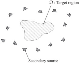
Let Ω ⊂ R 3 be a target region for synthesizing the desired sound field. As shown in Fig. 1, L secondary sources are placed at r l ∈ R 3 \ Ω ( l ∈ { 1 , . . . , L } ). The driving signal of the l th secondary source and its transfer function to the position r ∈ Ω at the angular frequency ω are denoted as d l ( ω ) and g l ( r , ω ) , respectively. Then, the synthesized pressure distribution u syn ( r , ω ) ( r ∈ Ω ) is represented as
<!-- formula-not-decoded -->
where g ( r , ω ) ∈ C L and d ( ω ) ∈ C L are the vectors consisting of g l ( r , ω ) and d l ( ω ) , respectively. Hereafter, ω is omitted for notational simplicity.
The objective is to synthesize the desired sound field u des ( r ) over the target region Ω . We define the optimization problem to obtain d as follows.
<!-- formula-not-decoded -->
Figure 1: Sound field synthesis over the target region Ω with multiple loudspeakers
<details>
<summary>Image 1 Details</summary>
### Visual Description
## Diagram: Spatial Distribution of Secondary Sources and Target Region
### Overview
The diagram illustrates a spatial arrangement of 12 secondary sources surrounding a central target region (Ω). The target region is depicted as an irregularly shaped area with a dotted outline, while the secondary sources are represented as uniformly sized, cone-shaped icons positioned at equidistant intervals around the perimeter. Arrows indicate directional flow or influence from the secondary sources toward the target region.
### Components/Axes
- **Labels**:
- **Ω**: Target region (central shaded area with dotted boundary).
- **Secondary source**: Cone-shaped icons (12 instances).
- **Legend**: Not explicitly present; labels are directly annotated on the diagram.
- **Spatial Grounding**:
- **Target region (Ω)**: Centered in the diagram, occupying ~60% of the vertical space and ~50% of the horizontal space.
- **Secondary sources**: Arranged in a circular pattern around Ω, with 12 evenly spaced instances. Each source is positioned at a radial distance of ~1.5× the radius of Ω.
- **Arrows**: Originate from the base of each secondary source and point toward the target region.
### Detailed Analysis
- **Secondary sources**:
- 12 identical cone-shaped icons, uniformly gray in color.
- Positioned at 30° intervals (360°/12) around the target region.
- No numerical identifiers or categorical labels assigned to individual sources.
- **Target region (Ω)**:
- Irregular polygonal shape with a dotted boundary.
- Shaded with diagonal hatching (45° orientation).
- No internal labels or subdivisions.
- **Arrows**:
- Thin, straight lines connecting secondary sources to Ω.
- Uniform thickness and style across all 12 connections.
### Key Observations
1. **Symmetry**: Secondary sources are evenly distributed around Ω, suggesting a designed or optimized layout.
2. **Directionality**: Arrows imply a unidirectional relationship (e.g., data flow, resource allocation, or influence).
3. **No numerical data**: The diagram lacks quantitative values, scales, or categorical legends beyond the two labels (Ω and secondary source).
### Interpretation
The diagram likely represents a system where secondary sources (e.g., sensors, transmitters, or processing units) contribute to or interact with a central target region (e.g., a processing hub, data sink, or area of interest). The absence of numerical data suggests the focus is on spatial relationships rather than quantitative metrics. The directional arrows imply a dependency or flow from the periphery (secondary sources) to the core (target region), which could model scenarios such as:
- **Resource distribution**: Secondary sources supplying inputs to a central system.
- **Network topology**: Peripheral nodes communicating with a central node.
- **Environmental monitoring**: Sensors surrounding a region of interest (e.g., a pollution hotspot).
The irregular shape of Ω may indicate a non-uniform area of interest, while the uniform placement of secondary sources suggests a deliberate design to ensure coverage or redundancy. The lack of a legend or scale limits quantitative interpretation but emphasizes the conceptual relationship between components.
</details>
Since this problem is difficult to solve owing to the regional integration, several methods to approximately solve it, for example, (weighted) pressure and mode matching [1-6], have been proposed.
## 2.1. Pressure Matching
Pressure matching is one of the widely used sound field synthesis methods to approximately solve (2). First, the region Ω is discretized into N control points whose positions are denoted as { r n } N n =1 . We assume that the control points are arranged densely enough over Ω . Then, the cost function for pressure matching is formulated as the minimization problem of the squared error between the synthesized and desired pressures at the control points as
<!-- formula-not-decoded -->
where G ∈ C N × L is the matrix consisting of transfer functions { g l ( r n ) } N n =1 , u des ∈ C N is the vector consisting of the desired pressures { u des ( r n ) } N n =1 , and β is the regularization parameter. This least-squares problem (3) has a closed-form solution as follows:
<!-- formula-not-decoded -->
Pressure matching is extended as weighted pressure matching [6, 18] by combining with sound field interpolation techniques [19,20].
Another strategy to approximate Q ( d ) is to represent the sound field by spherical wavefunction expansion [21, 22], which is referred to as (weighted) mode matching [4, 5]. It is demonstrated that weighted pressure matching is a special case of weighted mode matching in [6].
## 2.2. Spatial Aliasing Artifacts
On the basis of the single-layer potential [21,23], the desired sound field can be perfectly synthesized if secondary sources are continuously distributed point sources on a surface of the target region Ω . However, owing to the discrete placement of the secondary sources, spatial aliasing artifacts are unavoidable for sound field synthesis methods. The synthesis accuracy can decrease particularly at high frequencies, which can lead to the degradation of sound localization and the coloration of source signals. The properties of spatial aliasing in analytical sound field synthesis methods have been extensively investigated [24], but spatial aliasing can also occur in numerical methods, depending on the secondary source placement [25, 26]. One of the strategies to improve the synthesis accuracy at high frequencies is to make the target region smaller [5,27]. The challenge here is to improve the perceptual quality of the synthesized sound field by mitigating spatial aliasing artifacts in a broad listening area.
## 3. PROPOSED METHOD BASED ON COMBINATION OF PRESSURE AND AMPLITUDE MATCHING
Even when it is difficult to synthesize the desired pressure distribution, i.e., amplitude and phase, for high frequencies, it can be considered that synthesizing only the amplitude distribution can be achieved by leaving the phase distribution arbitrary. On the basis of the human's auditory properties, ILD is known to be a dominant cue for horizontal sound localization above 1500 Hz , and the dependence on ITD is markedly reduced from 1000 -1500 Hz [16,17], which indicates that synthesizing the amplitude distribution is sufficient for sound localization above 1500 Hz . This perceptual property is also used in a method for binaural rendering [28]. Furthermore, coloration effects can be alleviated by reproducing the flat amplitude response as much as possible. Therefore, we propose a method combining amplitude matching [14, 15], which is aimed to synthesize the desired amplitude at the control points, with pressure matching. By applying amplitude matching for high frequencies, the parameters to be controlled can be reduced from pressure matching, keeping the range of the target region, i.e., the number of control points. Thus, we can improve the perceptual quality of the synthesized sound field by reproducing a more accurate amplitude distribution over Ω .
## 3.1. Proposed Algorithm
We define the optimization problem of the proposed method as a composite of pressure and amplitude matching as
<!-- formula-not-decoded -->
where |·| represents the element-wise absolute value of vectors, and γ ∈ R ([0 , 1]) is the parameter that determines the balance between pressure and amplitude matching. When γ = 0 , (5) corresponds to pressure matching, and when γ = 1 , it corresponds to amplitude matching; therefore, γ should be set close to 0 for low frequencies and 1 for high frequencies. For example, γ can be defined as a sigmoid function of ω with the transition angular frequency ω T and parameter σ as
<!-- formula-not-decoded -->
Since the cost function J in (5) is neither convex nor differentiable owing to the squared error term of the amplitude matching, (5) does not have a closed-form solution. However, the alternating direction method of multipliers (ADMM) can be applied in a similar manner to the algorithm for amplitude matching [15]. First, we introduce the auxiliary variables of amplitude a ∈ R N ≥ 0 and phase θ ∈ R N such that Gd = a /circledot e j θ , where /circledot represents the Hadamard product. Then, (5) is reformulated as
<!-- formula-not-decoded -->
The augmented Lagrangian function L ρ for (7) is defined as
<!-- formula-not-decoded -->
where λ ∈ C N is the Lagrange multiplier, /Rfractur [ · ] represents the real part of a complex value, and ρ > 0 is the penalty parameter.
Each variable is alternately updated on the basis of ADMM as
<!-- formula-not-decoded -->
<!-- formula-not-decoded -->
<!-- formula-not-decoded -->
where i denotes the iteration index. (9) is minimized independently for θ and a as
<!-- formula-not-decoded -->
<!-- formula-not-decoded -->
The update rule for d is obtained by solving (10) as
<!-- formula-not-decoded -->
By iteratively updating θ ( i ) , a ( i ) , d ( i ) , and λ ( i ) by using (12), (13), (14), and (11), respectively, starting with initial values, we can obtain the optimal driving signal d .
## 3.2. Time-Domain Filter Design
By using the proposed algorithm described in Sect. 3.1, we can obtain the driving signal in the frequency domain. In practice, a finite impulse response (FIR) filter is obtained by computing the inverse Fourier transform of d for target frequency bins. However, if the driving signal is independently determined for each frequency, it can have discontinuities between frequency bins particularly for γ = 1 because the phase of d is arbitrary. These discontinuities can lead to an unnecessarily large FIR filter length.
To overcome this issue, the differential-norm penalty, which is also used in amplitude matching [15], can be applied. By introducing the subscript of the index of the frequency bin f ∈ { 1 , . . . , F } , we define the differential-norm penalty for the f th frequency bin as
<!-- formula-not-decoded -->
The optimization problem for the time-domain filter design is represented as
<!-- formula-not-decoded -->
where α is the weight for the differential-norm penalty term. ADMM is similarly applied to solve (16), but its detailed derivation is omitted. The derivation of ADMM for amplitude matching and a technique to reduce computational complexity can be found in [15].
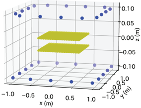
Figure 2: Experimental setup. Blue circles and yellow dots represent sources and control points, respectively.
<details>
<summary>Image 2 Details</summary>
### Visual Description
## 3D Coordinate System Diagram: Sensor Network and Data Collection Zones
### Overview
The image depicts a 3D coordinate system with labeled axes (x, y, z) and two distinct elements: blue circular markers (sensor nodes) and yellow planar regions (data collection zones). The spatial arrangement suggests a technical setup for environmental monitoring or spatial data analysis.
### Components/Axes
- **Axes**:
- **x-axis**: Labeled "x (m)" with range -1.0 to 1.0 meters.
- **y-axis**: Labeled "y (m)" with range -1.0 to 1.0 meters.
- **z-axis**: Labeled "z (m)" with range -0.10 to 0.10 meters.
- **Legend**:
- **Blue dots**: Labeled "Sensor Nodes" (positioned at grid intersections and perimeter).
- **Yellow planes**: Labeled "Data Collection Zones" (two horizontal layers).
### Detailed Analysis
- **Sensor Nodes (Blue Dots)**:
- Distributed across the grid with approximate coordinates:
- Perimeter: (-1.0, -1.0, -0.10), (1.0, -1.0, -0.10), (-1.0, 1.0, -0.10), (1.0, 1.0, -0.10).
- Interior: (-0.5, 0.0, 0.05), (0.5, 0.0, 0.05), (0.0, -0.5, -0.05), (0.0, 0.5, -0.05).
- Uniform spacing suggests a structured grid pattern.
- **Data Collection Zones (Yellow Planes)**:
- **Top plane**: Positioned at z ≈ 0.00 meters, spanning x: -0.5 to 0.5 and y: -0.5 to 0.5.
- **Bottom plane**: Positioned at z ≈ -0.05 meters, spanning the same x and y range as the top plane.
- Both planes are parallel to the xy-plane and offset vertically.
### Key Observations
1. **Spatial Distribution**: Sensor nodes are concentrated at grid intersections and perimeter edges, with fewer nodes in the interior.
2. **Layered Zones**: The two yellow planes are separated by 0.05 meters vertically, indicating distinct data collection layers.
3. **Symmetry**: The setup exhibits symmetry about the z-axis, with mirrored sensor node placements.
### Interpretation
The diagram likely represents a **sensor network architecture** for monitoring environmental parameters (e.g., temperature, humidity) across a defined spatial grid. The **blue dots** (sensor nodes) are strategically placed to cover the perimeter and interior, ensuring comprehensive data coverage. The **yellow planes** (data collection zones) may represent regions of interest where data aggregation or analysis occurs, possibly simulating layered environmental strata (e.g., surface vs. subsurface measurements). The absence of dynamic trends (e.g., time-dependent data) suggests this is a static schematic for system design rather than real-time data visualization. The symmetry and grid alignment imply a focus on precision and uniformity in data collection.
</details>
## 4. EXPERIMENTS
We conducted experiments to evaluate the proposed method (Proposed) compared with pressure matching (PM). First, numerical experimental results are shown to evaluate the ILD of a listener and the amplitude response of the synthesized sound field. Second, the results of listening experiments using a practical system are presented.
## 4.1. Numerical Experiments
Numerical experiments in the frequency domain were conducted under the three-dimensional free-field assumption. The target region Ω was a cuboid of 1 . 0 m × 1 . 0 m × 0 . 04 m . As shown in Fig. 2, 16 omnidirectional loudspeakers were placed along the borders of the squares of 2 . 0 m × 2 . 0 m at the heights of z = ± 0 . 1 m , and 24 × 24 × 2 control points were regularly placed inside Ω . Therefore, the total number of loudspeakers and control points were L = 32 and N = 1152 , respectively. The desired sound field was a spherical wave from the point source at (2 . 0 , 0 . 0 , 0 . 0) m . In Proposed, γ was set using (6) with ω T / 2 π = 2000 and σ = 0 . 01 so that the phase distribution becomes arbitrary above 2000 Hz . The regularization parameter β for Proposed and PM was set as ‖ G H G ‖ 2 2 × 10 -3 . The penalty parameter ρ in (8) was 1 . 0 .
We evaluated the ILDs of the synthesized sound field when a listener's head was in Ω . The binaural signals at ω for the position r H ∈ Ω and azimuth direction φ H ∈ [0 , 2 π ) of the listener's head were denoted as b L ( r H , φ H , ω ) and b R ( r H , φ H , ω ) for the left and right ears, respectively. b L and b R were obtained by calculating the transfer function between the loudspeakers and the listener's ears using Mesh2HRTF [29,30]. The ILD for r H and φ H was calculated in the frequency domain as
<!-- formula-not-decoded -->
The evaluation measure was the normalized error ( NE ) between the synthesized and desired ILDs ( ILD syn and ILD true , respectively) at r H defined as
<!-- formula-not-decoded -->
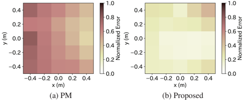
where the summation for φ H was calculated for { 0 , π/ 32 , π/ 16 , . . . , 31 π/ 32 } rad . The distributions of NE( r H ) on the x -y -plane at z = 0 for Proposed and PM are shown in Fig. 3. The evaluated positions were 5 × 5 points on the square of
Figure 3: Distribution of NE of ILDs.
<details>
<summary>Image 3 Details</summary>
### Visual Description
## Heatmaps: Normalized Error Distribution Comparison
### Overview
The image presents two side-by-side heatmaps comparing normalized error distributions across a 2D spatial grid. The left heatmap (a) represents a baseline method labeled "PM," while the right heatmap (b) represents a "Proposed" method. Both maps use color gradients to encode error magnitudes, with darker red indicating higher errors and lighter yellow indicating lower errors.
### Components/Axes
- **X-axis**: Labeled "x (m)" with values ranging from -0.4 m to 0.4 m in 0.2 m increments.
- **Y-axis**: Labeled "y (m)" with values ranging from -0.4 m to 0.4 m in 0.2 m increments.
- **Color Scale**: Shared legend on the right of each heatmap, labeled "Normalized Error" with values from 0.0 (light yellow) to 1.0 (dark red).
- **Legend Positioning**: Right-aligned for both heatmaps, occupying ~20% of the total width.
### Detailed Analysis
#### (a) PM Heatmap
- **Top-left quadrant** (x: -0.4 to 0.0, y: 0.0 to 0.4): Dominated by dark red cells, indicating normalized errors near 0.8–1.0.
- **Bottom-left quadrant** (x: -0.4 to 0.0, y: -0.4 to 0.0): Mixed red and orange cells, with errors ranging from 0.4–0.8.
- **Top-right quadrant** (x: 0.0 to 0.4, y: 0.0 to 0.4): Gradual transition from orange to light yellow, errors ~0.2–0.6.
- **Bottom-right quadrant** (x: 0.0 to 0.4, y: -0.4 to 0.0): Predominantly light yellow, errors ~0.0–0.4.
#### (b) Proposed Heatmap
- **Uniform distribution**: Most cells are light yellow, with errors clustered near 0.0–0.2.
- **Top-left quadrant**: Slightly darker yellow cells (errors ~0.2–0.4) compared to the rest.
- **No dark red regions**: No areas exceed 0.4 normalized error.
### Key Observations
1. The PM method exhibits significant spatial variability in error, with high errors concentrated in the top-left and bottom-left quadrants.
2. The Proposed method shows a drastic reduction in error magnitude, with nearly uniform low errors across the grid.
3. The top-left quadrant of the PM heatmap contains the highest errors (~0.8–1.0), while the Proposed method reduces these to ~0.2–0.4.
### Interpretation
The Proposed method demonstrates a consistent improvement in error reduction compared to the PM baseline. The PM method’s high errors in specific quadrants suggest systematic biases or limitations in handling certain spatial regions. The Proposed method’s uniformity implies a more robust or adaptive approach, potentially addressing the PM method’s weaknesses. The absence of dark red regions in the Proposed heatmap indicates a significant performance gain, particularly in error-prone areas. This suggests the Proposed method may be more reliable for applications requiring precise spatial error control.
</details>
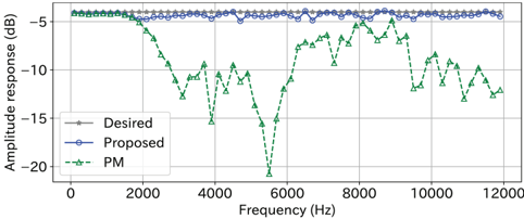
Figure 4: Amplitude responses of desired and synthesized sound fields at the center of Ω .
<details>
<summary>Image 4 Details</summary>
### Visual Description
## Line Graph: Amplitude Response vs. Frequency
### Overview
The image is a line graph comparing three amplitude response curves across a frequency range. The graph shows three data series: "Desired" (gray stars), "Proposed" (blue circles), and "PM" (green triangles). The x-axis represents frequency (Hz), and the y-axis represents amplitude response (dB). The graph highlights deviations between the proposed system and the desired performance, as well as the performance of a PM (possibly a physical or mathematical model).
### Components/Axes
- **X-axis (Frequency)**: Labeled "Frequency (Hz)" with a range from 0 to 12,000 Hz. Tick marks are at 0, 2000, 4000, 6000, 8000, 10,000, and 12,000 Hz.
- **Y-axis (Amplitude Response)**: Labeled "Amplitude response (dB)" with a range from -20 dB to -5 dB. Tick marks are at -20, -15, -10, -5 dB.
- **Legend**: Located in the bottom-left corner, with three entries:
- **Desired**: Gray stars (solid line).
- **Proposed**: Blue circles (dashed line).
- **PM**: Green triangles (dotted line).
### Detailed Analysis
1. **Desired (Gray Stars)**:
- A flat, horizontal line at approximately **-5 dB** across all frequencies.
- No variation observed; represents the target amplitude response.
2. **Proposed (Blue Circles)**:
- Slightly above the Desired line, with minor fluctuations.
- Amplitude response ranges between **-5 dB and -4 dB**.
- Peaks at ~-4 dB near 2000 Hz and 10,000 Hz.
- Dips to ~-5.5 dB near 6000 Hz.
3. **PM (Green Triangles)**:
- Highly variable, with sharp dips and peaks.
- Amplitude response ranges from **-5 dB to -18 dB**.
- Sharp drop to **-15 dB** near 4000 Hz.
- Another dip to **-18 dB** near 6000 Hz.
- Peaks at **-5 dB** near 8000 Hz and 10,000 Hz.
- Ends at ~-12 dB at 12,000 Hz.
### Key Observations
- The **Desired** line is perfectly flat, indicating an idealized target.
- The **Proposed** line closely follows the Desired line but shows minor deviations, suggesting a near-optimal but imperfect system.
- The **PM** line exhibits significant instability, with large deviations from the Desired line, particularly at 4000 Hz and 6000 Hz. This suggests the PM model or system has critical performance issues at these frequencies.
### Interpretation
The graph demonstrates a comparison between a target (Desired), a proposed solution (Proposed), and a physical/mathematical model (PM). The Proposed system performs well but does not fully meet the Desired target, while the PM model shows severe instability, likely due to design flaws or unaccounted variables. The PM's sharp dips at 4000 Hz and 6000 Hz may indicate resonance issues, filtering errors, or modeling inaccuracies. The Proposed system’s minor fluctuations suggest it could be optimized further to align more closely with the Desired line. The PM’s performance highlights the need for refinement in its design or implementation.
</details>
1 . 0 m × 1 . 0 m . The NE of Proposed was smaller than that of PM over the region. Note that the ITDs were accurately synthesized in both methods below 2000 Hz .
Next, the amplitude response of the synthesized sound field was investigated. In Fig. 4, the amplitude responses at the center of Ω of the desired sound field and synthesized sound field of Proposed and PM are plotted. Owing to the large variations in the amplitude response of PM above 2000 Hz , the timbre of the source signal can be highly distorted. In contrast, the almost flat amplitude response was achieved by Proposed at the center of Ω .
## 4.2. Listening Experiments
Listening experiments were conducted to evaluate the perceptual quality of the synthesized sound field by using a practical loudspeaker array. The numbers and positions of loudspeakers and control points were the same as those in Fig. 2. The reference loudspeaker was placed at (2 . 0 , 0 . 5 , 0 . 0) m as a primary sound source of the desired field. The driving signals of Proposed and PM were obtained by assuming the loudspeakers as point sources. The reverberation time T 60 of the room was around 0 . 19 s .
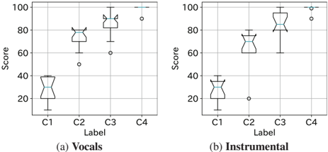
The perceptual quality was evaluated by using multiple stimuli with a hidden reference and anchor (MUSHRA) [31]. Test participants were asked to rate the difference between the reference and test signals of 10 s on a scale from 0 to 100. The reference and test signals are summarized as follows:
- Reference: The source signal played back through the reference loudspeaker.
- C1/Hidden anchor: The lowpass-filtered source signal up to 3 . 5 kHz played back through the reference loudspeaker.
- C2/PM: The sound synthesized by PM and played back through the loudspeaker array.
- C3/Proposed: The sound synthesized by Proposed and played
Figure 5: Box-and-whisker plots of scores for each test signal. Circles indicate outliers, and the notches represent 95% confidence intervals of the median.
<details>
<summary>Image 5 Details</summary>
### Visual Description
## Box Plots: Vocal and Instrumental Scores by Category
### Overview
The image contains two side-by-side box plots comparing scores across four categories (C1, C2, C3, C4) for two groups: **Vocals** (left) and **Instrumental** (right). Scores range from 0 to 100 on the y-axis. Each box plot displays medians (blue lines), interquartile ranges (boxes), and outliers (dots). The data suggests performance trends across categories for both groups.
---
### Components/Axes
- **X-axis (Categories)**: Labeled C1, C2, C3, C4 (no explicit legend, but categories are consistent across both plots).
- **Y-axis (Score)**: Numerical scale from 0 to 100, with gridlines at 20-unit intervals.
- **Legend**: Not explicitly present, but the two plots are labeled **(a) Vocals** and **(b) Instrumental** as figure captions.
- **Outliers**: Represented as dots outside the whiskers in both plots.
---
### Detailed Analysis
#### Vocals (a)
- **C1**: Median ~30, IQR ~20–40, outliers at ~50 and ~10.
- **C2**: Median ~70, IQR ~60–80, outliers at ~50 and ~90.
- **C3**: Median ~85, IQR ~75–90, outliers at ~60 and ~95.
- **C4**: Median ~95, IQR ~90–100, no visible outliers.
#### Instrumental (b)
- **C1**: Median ~30, IQR ~20–40, outliers at ~10 and ~50.
- **C2**: Median ~65, IQR ~50–75, outliers at ~20 and ~80.
- **C3**: Median ~85, IQR ~75–90, outliers at ~60 and ~95.
- **C4**: Median ~95, IQR ~90–100, outliers at ~85 and ~100.
---
### Key Observations
1. **Upward Trend**: Both groups show increasing median scores from C1 to C4.
2. **Variability**: Vocals exhibit wider spreads in C1 and C2, while Instrumental scores are more consistent in C3 and C4.
3. **Outliers**:
- Vocals: Notable outliers in C2 (~90) and C3 (~60).
- Instrumental: Outliers in C4 (~85, ~100) suggest exceptional cases.
4. **Overlap**: Medians for C3 and C4 are nearly identical between the two groups (~85–95).
---
### Interpretation
- **Performance Improvement**: The consistent rise in medians across categories implies progression or mastery over time, possibly reflecting skill development or increasing difficulty.
- **Vocals vs. Instrumental**:
- Vocals show higher variability in early categories (C1–C2), suggesting less consistency in foundational skills.
- Instrumental scores stabilize in later categories (C3–C4), indicating more reliable performance at advanced levels.
- **Outliers**: The presence of high outliers in C4 for both groups may represent exceptional talent or measurement anomalies. The low outlier in Vocals C3 (~60) could indicate a regression or unique challenge.
This analysis highlights how categorical performance metrics can reveal trends in skill acquisition, consistency, and outliers in artistic disciplines.
</details>
back through the loudspeaker array.
- C4/Hidden reference: The same as Reference.
The participants' head center was approximately positioned at the center of the target region by adjusting the chair, but they were able to rotate and move their heads on the chair freely. The participants were able to listen to each test signal repeatedly. Fourteen male subjects in their 20s and 30s were included, and those who scored more than 60 on the hidden anchor, which was one participant in this test, were excluded from the evaluation. Two source signals, Vocals and Instrumental , taken from track 10 of MUSDB18-HQ [32] were investigated.
Fig. 5 shows the box-and-whisker plots of the scores of each test signal. The median score of Proposed was significantly higher than that of PM for both Vocals and Instrumental . After the validation of the normality of data for C2 and C3 by the Shapiro-Wilk test, Welch's t -test was conducted at a significance level of 0 . 05 . The p values for Vocals and Instrumental were 9 . 1 × 10 -4 and 2 . 0 × 10 -3 , respectively; therefore, there were significant differences in mean scores between C2 and C3 in the both cases.
## 5. CONCLUSION
We proposed a sound field synthesis method based on the combination of pressure and amplitude matching to improve perceptual quality. The cost function is defined as square errors of pressure distribution for low frequencies and amplitude distribution for high frequencies to alleviate the effects of spatial aliasing artifacts. The ADMM-based algorithm to solve this cost function is also derived. In the numerical experiments and listening experiments, it was validated that the perceptual quality of the proposed method can be improved from that of PM. Future work includes extended listening experiments to evaluate perceptual quality in more detail.
## 6. ACKNOWLEDGMENT
This work was supported by JSPS KAKENHI Grant Number 22H03608 and JST FOREST Program Grant Number JPMJFR216M, Japan.
## 7. REFERENCES
- [1] P. A. Nelson, 'Active control of acoustic fields and the reproduction of sound,' J. Sound Vibr. , vol. 177, no. 4, pp. 447-477, 1993.
- [2] O. Kirkeby, P. A. Nelson, F. O. Bustamante, and H. Hamada, 'Local sound field reproduction using digital signal processing,' J. Acoust. Soc. Amer. , vol. 100, no. 3, pp. 1584-1593, 1996.
- [3] T. Betlehem and T. D. Abhayapala, 'Theory and design of sound field reproduction in reverberant rooms,' J. Acoust. Soc. Amer. , vol. 117, no. 4, pp. 2100-2111, Apr. 2005.
- [4] M. A. Poletti, 'Three-dimensional surround sound systems based on spherical harmonics,' J. Audio Eng. Soc. , vol. 53, no. 11, pp. 1004-1025, Nov. 2005.
- [5] N. Ueno, S. Koyama, and H. Saruwatari, 'Three-dimensional sound field reproduction based on weighted mode-matching method,' IEEE/ACM Trans. Audio, Speech, Lang. Process. , vol. 27, no. 12, pp. 1852-1867, 2019.
- [6] S. Koyama, K. Kimura, and N. Ueno, 'Weighted pressure and mode matching for sound field reproduction: Theoretical and experimental comparisons,' J. Audio Eng. Soc. , vol. 71, no. 4, pp. 173-185, 2023.
- [7] A. J. Berkhout, D. de Vries, and P. Vogel, 'Acoustic control by wave field synthesis,' J. Acoust. Soc. Amer. , vol. 93, no. 5, pp. 2764-2778, 1993.
- [8] S. Spors, R. Rabenstein, and J. Ahrens, 'The theory of wave field synthesis revisited,' in Proc. 124th AES Conv. , Amsterdam, Netherlands, Oct. 2008.
- [9] J. Daniel, S. Moureau, and R. Nicol, 'Further investigations of high-order ambisonics and wavefield synthesis for holophonic sound imaging,' in Proc. 114th AES Conv. , Amsterdam, Netherlands, Mar. 2003.
- [10] J. Ahrens and S. Spors, 'An analytical approach to sound field reproduction using circular and spherical loudspeaker distributions,' Acta Acustica united with Acustica , vol. 94, no. 6, pp. 988-999, Nov. 2008.
- [11] Y. J. Wu and T. D. Abhayapala, 'Theory and design of soundfield reproduction using continuous loudspeaker concept,' IEEE Trans. Audio, Speech, Lang. Process. , vol. 17, no. 1, pp. 107-116, Jan. 2009.
- [12] S. Koyama, K. Furuya, Y. Hiwasaki, and Y. Haneda, 'Analytical approach to wave field reconstruction filtering in spatiotemporal frequency domain,' IEEE Trans. Audio, Speech, Lang. Process. , vol. 21, no. 4, pp. 685-696, 2013.
- [13] S. Koyama, K. Furuya, Y. Hiwasaki, Y. Haneda, and Y. Suzuki, 'Wave field reconstruction filtering in cylindrical harmonic domain for with-height recording and reproduction,' IEEE/ACM Trans. Audio, Speech, Lang. Process. , vol. 22, no. 10, pp. 1546-1557, 2014.
- [14] S. Koyama, T. Amakasu, N. Ueno, and H. Saruwatari, 'Amplitude matching: Majorization-minimization algorithm for sound field control only with amplitude constraint,' in Proc. IEEE Int. Conf. Acoust., Speech, Signal Process. (ICASSP) , Jun. 2021, pp. 411-415.
- [15] T. Abe, S. Koyama, N. Ueno, and H. Saruwatari, 'Amplitude matching for multizone sound field control,' IEEE/ACM Trans. Audio, Speech, Lang. Process. , vol. 31, pp. 656-669, 2023.
- [16] J. Blauert, Spatial Hearing: The Psychophysicas of Human Sound Localization . Cambridge: The MIT Press, 1997.
- [17] A. Brughera, L. Dunai, and W. M. Hartmann, 'Human interaural time difference thresholds for sine tones: The highfrequency limit,' J. Acoust. Soc. Amer. , pp. 2839-2855, 2013.
- [18] S. Koyama and K. Arikawa, 'Weighted pressure matching based on kernel interpolation for sound field reproduction,' in Proc. Int. Congr. Acoust. (ICA) , Gyeongju, Republic of Korea, Oct. 2022.
- [19] N. Ueno, S. Koyama, and H. Saruwatari, 'Sound field recording using distributed microphones based on harmonic analysis of infinite order,' IEEE Signal Process. Lett. , vol. 25, no. 1, pp. 135-139, 2018.
- [20] --, 'Directionally weighted wave field estimation exploiting prior information on source direction,' IEEE Trans. Signal Process. , vol. 69, pp. 2383-2395, 2021.
- [21] E. G. Williams, Fourier Acoustics: Sound Radiation and Nearfield Acoustical Holography . London, UK: Academic Press, 1999.
- [22] P. A. Martin, Multiple Scattering: Interaction of TimeHarmonic Waves with N Obstacles . New York: Cambridge University Press, 2006.
- [23] D. Colton and R. Kress, Inverse Acoustic and Electromagnetic Scattering Theory . New York, NY, USA: Springer, 2013.
- [24] S. Spors and R. Rabenstein, 'Spatial aliasing artifacts produced by linear and circular loudspeaker arrays used for wave field synthesis,' in Proc. 120th AES Conv. , May 2006.
- [25] S. Koyama, G. Chardon, and L. Daudet, 'Optimizing source and sensor placement for sound field control: An overview,' IEEE/ACM Trans. Audio, Speech, Lang. Process. , vol. 28, pp. 686-714, 2020.
- [26] K. Kimura, S. Koyama, N. Ueno, and H. Saruwatari, 'Meansquare-error-based secondary source placement in sound field synthesis with prior information on desired field,' in Proc. IEEE Int. Workshop Appl. Signal Process. Audio Acoust. (WASPAA) , Oct. 2021, pp. 281-285.
- [27] M. Poletti and T. Betlehem, 'Creation of a single sound field for multiple listeners,' in Proc. INTER-NOISE , 2014, pp. 2033-2040.
- [28] C. Scho¨ orkhuber, M. Zaynschirm, and R. H oldrich, 'Binaural rendering of ambisonics signals via magnitude least squares,' in Proc. DAGA , 2018, pp. 339-342.
- [29] H. Ziegelwanger, W. Kreuzer, and P. Majdak, 'Mesh2hrtf: Open-source software package for the numerical calculation of head-related transfer functions,' in Proc. Int. Congr. Sound Vibr. (ICSV) , 2015.
- [30] H. Ziegelwanger, P. Majdak, and W. Kreuzer, 'Numerical calculation of listener-specific head-related transfer functions and sound localization: Microphone model and mesh discretization,' J. Acoust. Soc. Amer. , vol. 138, no. 1, pp. 208222, 2015.
- [31] International Telecommunication Union, Radiocommunication Sector, 'Recommendation itu-r bs.1534-3: Method for the subjective assessment of intermediate quality level of audio systems,' 2014.
- [32] Z. Rafii, A. Liutkus, F.-R. St¨ oter, S. I. Mimilakis, and R. Bittner, 'MUSDB18-HQ - an uncompressed version of MUSDB18,' Dec. 2019. [Online]. Available: https://doi.org/10.5281/zenodo.3338373