# SimLOD: Simultaneous LOD Generation and Rendering
## SimLOD: Simultaneous LOD Generation and Rendering
Markus Schütz, Lukas Herzberger, Michael Wimmer
TU Wien
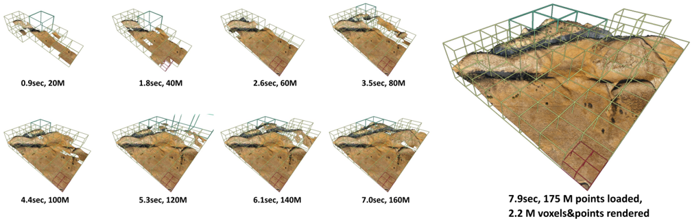
Figure 1: State-of-the-art LOD generation approaches require users to wait until the entire data set is processed before they are able to view it. Our approach incrementally constructs an LOD structure directly on the GPU while points are being loaded from disk, and immediately displays intermediate results. Loading the depicted point cloud was bottlenecked to 22M points/sec by the industry-standard but CPUintensive compression format (LAZ). Our approach is able to handle up to 580M points/sec while still rendering the loaded data in real time.
<details>
<summary>Image 1 Details</summary>
### Visual Description
\n
## Diagram: Progressive Mesh Loading & Rendering
### Overview
The image depicts a series of nine isometric views of a 3D mesh representing a terrain or excavation site. Each view shows the mesh at a different stage of loading and rendering, indicated by the time elapsed and the number of points/voxels loaded. The views are arranged horizontally across two rows, demonstrating the progressive refinement of the model as more data is processed. A wireframe cube surrounds the mesh in each view, likely representing the bounding volume or loading area.
### Components/Axes
There are no explicit axes or legends in the traditional sense. The data is presented visually through the progression of the mesh and accompanying text labels. The key parameters displayed are:
* **Time (seconds):** Indicates the time taken to reach a particular loading/rendering state.
* **Points/Voxels (Millions):** Indicates the number of points loaded or voxels rendered.
### Detailed Analysis or Content Details
The image shows the following stages of loading and rendering:
1. **0.9 sec, 20M:** The initial state, showing a very sparse mesh.
2. **1.8 sec, 40M:** The mesh is becoming more defined, with more points loaded.
3. **2.6 sec, 60M:** Further refinement of the mesh.
4. **3.5 sec, 80M:** Continued increase in mesh density.
5. **4.4 sec, 100M:** The mesh is becoming more detailed.
6. **5.3 sec, 120M:** Further refinement of the mesh.
7. **6.1 sec, 140M:** Continued increase in mesh density.
8. **7.0 sec, 160M:** The mesh is becoming more detailed.
9. **7.9 sec, 175 M points loaded, 2.2 M voxels&points rendered:** The final state, showing a highly detailed mesh with a significant number of points loaded and voxels rendered. The red bounding box highlights a specific area of the mesh.
The wireframe cube appears to shrink in size relative to the mesh as more data is loaded, suggesting that the loading process is focused on filling the cube with detail. The darker areas within the mesh likely represent subsurface features or areas of shadow.
### Key Observations
* There is a roughly linear relationship between time elapsed and the number of points loaded/voxels rendered.
* The rate of increase in points/voxels appears to slow down slightly towards the end of the process.
* The final state (7.9 sec) shows a significantly more detailed mesh than the initial states.
* The red bounding box in the final image suggests a focus on a specific region of interest.
### Interpretation
This diagram demonstrates a progressive loading and rendering technique for a 3D mesh. The data suggests that the system is capable of efficiently loading and rendering large datasets, with a relatively smooth increase in detail over time. The linear relationship between time and data loaded indicates a consistent processing rate. The slowing down of the rate of increase towards the end could be due to factors such as increased rendering complexity or limitations in the rendering pipeline. The red bounding box suggests that the system may be optimized for rendering specific areas of interest within the mesh. This technique is likely used in applications such as terrain visualization, geological modeling, or archaeological reconstruction, where large datasets need to be rendered in real-time or near real-time. The progressive loading allows for a quick initial display of the model, followed by gradual refinement as more data becomes available.
</details>
## Abstract
About: We propose an incremental LOD generation approach for point clouds that allows us to simultaneously load points from disk, update an octree-based level-of-detail representation, and render the intermediate results in real time while additional points are still being loaded from disk. LOD construction and rendering are both implemented in CUDA and share the GPU's processing power, but each incremental update is lightweight enough to leave enough time to maintain real-time frame rates.
Background: LOD construction is typically implemented as a preprocessing step that requires users to wait before they are able to view the results in real time. This approach allows users to view intermediate results right away.
Results: Our approach is able to stream points from an SSD and update the octree on the GPU at rates of up to 580 million points per second (~9.3GB/s from a PCIe 5.0 SSD) on an RTX 4090. Depending on the data set, our approach spends an average of about 1 to 2 ms to incrementally insert 1 million points into the octree, allowing us to insert several million points per frame into the LOD structure and render the intermediate results within the same frame.
Discussion/Limitations: We aim to provide near-instant, real-time visualization of large data sets without preprocessing. Outof-core processing of arbitrarily large data sets and color-filtering for higher-quality LODs are subject to future work.
## CCS Concepts
- Computing methodologies → Rendering;
## 1. Introduction
Point clouds are an alternative representation of 3D models, comprising vertex-colored points without connectivity, and are typically obtained by scanning the real world via means such as laser scanners or photogrammetry. Since they are vertex-colored, large amounts of points are required to represent details that triangle meshes can cheaply simulate with textures. As such, point clouds are not an efficient representation for games, but they are nevertheless popular and ubiquitously available due to the need to scan real-world objects, buildings, and even whole countries.
Examples for massive point-cloud data sets include: The 3D Elevation Program (3DEP), which intends to scan the entire USA [3DEP], and Entwine[ENT], which currently hosts 53.6 trillion points that were collected in various individual scan campaigns within the 3DEP program [ENTW]. The Actueel Hoogtebestand Nederland (AHN) [AHN] program repeatedly scans the entire Netherlands, with the second campaign resulting in 640 billion points [AHN2], and the fourth campaign being underway. Many other countries also run their own country-wide scanning programs to capture the current state of land and infrastructure. At a smaller scale, buildings are often scanned as part of construction, planning, and digital heritage. But even though these are smaller in extent, they still comprise hundreds of millions to several billion points due to the higher scan density of terrestrial LIDAR and photogrammetry.
One of the main issues when working with large point clouds is the computational effort that is required to process and render hundreds of millions to billions of points. Level-of-detail structures are an essential tool to quickly display visible parts of a scene up to a certain amount of detail, thus reducing load times and improving rendering performance on lower-end devices. However, generating these structures can also be a time-consuming process. Recent GPU-based methods [SKKW23] improved LOD compute times down to a second per billion points, but they still require users to wait until the entire data set has been loaded and processed before the resulting LOD structure can be rendered. Thus, if loading a billion points takes 60 seconds plus 1 second of processing, users still have to wait 61 seconds to inspect the results.
In this paper, we propose an incremental LOD generation approach that allows users to instantly look at data sets as they are streamed from disk, without the need to wait until LOD structures are generated in advance. This approach is currently in-core, i.e., data sets must fit into memory, but we expect that it will serve as a basis for future out-of-core implementations to support arbitrarily large data sets.
Our contributions to the state-of-the-art are as follows:
- An approach that instantly displays large amounts of points as they are loaded from fast SSDs, and simultaneously updates an LOD structure directly on the GPU to guarantee high real-time rendering performance.
- As a smaller, additional contribution, we demonstrate that dynamically growing arrays of points via linked-lists of chunks can be rendered fairly efficiently in modern, compute-based rendering pipelines.
Specifically not a contribution is the development of a new LOD
structure. We generate the same structure as Wand et al. [WBB*08] or Schütz et al. [SKKW23], which are also very similar to the widely used modifiable nested octrees [SW11]. We opted for constructing the former over the latter because quantized voxels compress better than full-precision points (down to 10 bits per colored voxel), which improves the transfer speed of lower LODs over the network. Furthermore, since inner nodes are redundant, we can compute more representative, color-filtered values. However, both compression and color filtering are applied in post-processing before storing the results on disk and are not covered by this paper. This paper focuses on incrementally creating the LOD structure and its geometry as fast as possible for immediate display and picks a single color value from the first point that falls into a voxel cell.
## 2. Related Work
## 2.1. LOD Structures for Point Clouds
Point-based and hybrid LOD representations were initially proposed as a means to efficiently render mesh models at lower resolutions [RL00; CAZ01; CH02; DVS03] and possibly switch to the original triangle model at close-up views. With the rising popularity of 3D scanners that produce point clouds as intermediate and/or final results, these algorithms also became useful to handle the enormous amounts of geometry that are generated by scanning the real world. Layered point clouds (LPC) [GM04] was the first GPU-friendly as well as view-dependent approach, which made it suitable for visualizing arbitrarily large data sets. LPCs organize points into a multi-resolution binary tree where each node represents a part of the point cloud at a certain level of detail, with the root node depicting the whole data set at a coarse resolution, and child nodes adding additional detail in their respective regions. Since then, further research has improved various aspects of LPCs, such as utilizing different tree structures [WS06; WBB*08; GZPG10; OLRS23], improving LOD construction times [MVvM*15; KJWX19; SOW20; BK20; KB21] and higher-quality sampling strategies instead of selecting random subsets [vvL*22; SKKW23].
In this paper, we focus on constructing a variation of LPCs proposed by Wand et al. [WBB*08], which utilizes an octree where each node creates a coarse representation of the point cloud with a resolution of 128 3 cells, and leaf nodes store the original, fullprecision point data, as shown in Figure 2. Wand et al. suggest various primitives as coarse, representative samples (quantized points, Surfels, ...), but for this work we consider each cell of the 128 3 grid to be a voxel. A similar voxel-based LOD structure by Chajdas et al. [CRW14] uses 256 3 voxel grids in inner nodes and original triangle data in leaf nodes. Modifiable nested octrees (MNOs) [SW11] are also similar to the approach by Wand et al. [WBB*08], but instead of storing all points in leaves and representative samples (Surfels, Voxels, ...) in inner nodes, MNOs fill empty grid cells with points from the original data set.
Since our goal is to display all points the instant they are loaded from disk to GPU memory, we need LOD construction approaches that are capable of efficiently inserting new points into the hierarchy, expanding it if necessary, and updating all affected levels of detail. This disqualifies recent bottom-up or hybrid bottom-up and
top-down approaches [MVvM*15; SOW20; BK20; SKKW23] that achieve a high construction performance, but which require preprocessing steps that iterate through all data before they actually start with the construction of the hierarchy. Wand et al. [WBB*08] as well as Scheiblauer and Wimmer [SW11], on the other hand, propose modifiable LOD structures with deletion and insertion methods, which make these inherently suitable to our goal since we can add a batch of points, draw the results, and then add another batch of points. Bormann et al. [BDSF22] were the first to specifically explore this concept for point clouds by utilizing MNOs, but flushing updated octree nodes to disk that an external rendering engine can then stream and display. They achieved a throughput of 1.8 million points per second, which is sufficient to construct an LOD structure as fast as a laser scanner generates point data. A downside of these CPU-based approaches is that they do not parallelize well, as threads need to avoid processing the same node or otherwise sync critical operations. In this paper, we propose a GPU-friendly approach that allows an arbitrary amount of threads to simultaneously insert points, which allows us to construct and render on the same GPU at rates of up to 580 million points per second, or up to 1.2 billion points per second for construction without rendering.
While we focus on point clouds, there are some notable related works in other fields that allow simultaneous LOD generation and rendering. In general, any LOD structure with insertion operations can be assumed to fit these criteria, as long as inserting a meaningful amount of geometry can be done in milliseconds. Careil et al. [CBE20] demonstrate a voxel painter that is backed by a compressed LOD structure. We believe that Dreams - a popular 3D scene painting and game development tool for the PS4 - also matches the criteria, as developers reported experiments with LOD structures, and described the current engine as a 'cloud of clouds of point clouds" [Eva15].
## 2.2. Linked Lists
Linked lists are a well-known and simple structure whose constant insertion and deletion complexity, as well as the possibility to dynamically grow without relocation of existing data, make it useful as part of more complex data structures and algorithms (e.g.leastrecently-used (LRU) Caches [YMC02]). On GPUs, they can be used to realize order-independent transparency [YHGT10] by creating pixel-wise lists of fragments that can then be sorted and drawn front to back. In this paper, we use linked lists to append an unknown amount of points and voxels to octree nodes during LOD construction.
## 3. Data Structure
## 3.1. Octree
The LOD data structure we use is an octree-based [SW11] layered point cloud [GM04] with representative voxels in inner nodes and the original, full-precision point data in leaf nodes, which makes it essentially identical to the structures of Wand et al. [WBB*08] or Schütz et al. [SKKW23]. Leaf nodes store up to 50k points and inner nodes up to 128 3 (2M) voxels, but typically closer to 128 2 (16k) voxels due to the surfacic nature of point cloud data sets. The sparse nature of surface voxels is the reason why we store them in
<details>
<summary>Image 2 Details</summary>
### Visual Description
\n
## Photograph: Scene with Paved Ground and Barrels
### Overview
The image depicts a scene with a textured, paved ground surface. Two barrels, one red and one yellow, are positioned on a black metal stand at the upper-right of the frame. A small patch of green foliage is visible behind the barrels. The image appears to be a still life or a staged setup, likely for illustrative purposes.
### Components/Axes
There are no axes, scales, or legends present in this image. It is a photograph, not a chart or diagram.
### Detailed Analysis or Content Details
The ground surface is composed of irregularly shaped, grey stones or paving blocks. The texture is rough and uneven. The red barrel appears to be slightly taller than the yellow barrel. The metal stand supporting the barrels is simple in construction, consisting of vertical supports and a horizontal bar. The foliage is a dense, dark green. The lighting appears to be diffuse, with no strong shadows.
### Key Observations
The scene lacks any clear data points or measurable values. It is a visual representation of objects and textures. The arrangement of the barrels and foliage suggests a deliberate composition, but the purpose is unclear without additional context.
### Interpretation
The image does not present any data or trends for interpretation. It is a static visual scene. The combination of the rough paving, the industrial barrels, and the small patch of greenery could evoke themes of urban decay, resilience, or the juxtaposition of nature and industry. However, this is speculative without further information. The image is descriptive rather than analytical. It is a visual element that could be used to illustrate a concept or evoke a mood, but it does not contain inherent information to be extracted beyond its visual characteristics.
</details>
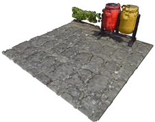
(a) Inner node with Voxels.
<details>
<summary>Image 3 Details</summary>
### Visual Description
\n
## Photograph: Two Industrial Filters
### Overview
The image depicts two cylindrical industrial filters, one red and one yellow, positioned side-by-side. Both filters appear to be filled with a white granular material, likely a filtration medium. The image does not contain any charts, graphs, or data tables. It is a visual representation of physical objects.
### Components/Axes
There are no axes, scales, or legends present in the image. The primary components are:
* **Red Filter:** A cylindrical filter with a textured surface, colored red. It has a slightly tapered shape, wider at the top.
* **Yellow Filter:** A cylindrical filter with a textured surface, colored yellow. It has a rectangular opening on its side.
* **Filtration Medium:** A white granular material filling the upper portion of both filters.
* **Base/Support:** The filters appear to be resting on a dark surface.
### Detailed Analysis or Content Details
The red filter is positioned slightly to the left and behind the yellow filter. The yellow filter has a visible rectangular opening on its side, approximately halfway down its height. Both filters have a textured surface, which may be designed to increase surface area or provide grip. The white granular material appears to be evenly distributed within the filters. The filters are approximately the same height, estimated to be around 60-80 cm. The diameter of each filter is estimated to be around 40-50 cm.
### Key Observations
The two filters are visually similar in shape and construction, differing primarily in color and the presence of the rectangular opening on the yellow filter. The granular material suggests these are used for solid-liquid or gas-solid separation.
### Interpretation
The image likely showcases different models or configurations of industrial filters. The color difference could indicate different materials of construction or intended applications. The opening on the yellow filter might be for inspection, maintenance, or to accommodate a specific connection. The filters are likely used in industrial processes to remove particulate matter from liquids or gases. Without additional context, it is difficult to determine the specific application or filtration process. The image serves as a visual representation of the equipment, rather than presenting any quantifiable data.
</details>
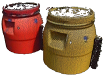
- (b) Leaf node with points.
Figure 2: (a) Close-up of a lower-resolution inner-node comprising 20 698 voxels that were sampled on a 128 3 grid. (b) A fullresolution leaf node comprising 22 858 points.
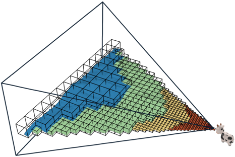
Figure 3: Higher-level octree nodes rendered closer to the camera. Inner nodes store lists of representative voxels that were sampled on a 128 3 grid, and leaf nodes store up to 50k full-precision points.
<details>
<summary>Image 4 Details</summary>
### Visual Description
\n
## 3D Heatmap: Conceptual Data Visualization
### Overview
The image depicts a three-dimensional heatmap represented as a grid of colored cubes within a transparent cubic frame. The color gradient transitions from blue (lower values) to green, then to yellow, and finally to red/brown (higher values). Two cow figurines are present in the bottom-right corner of the visualization. There are no explicit axis labels or numerical values provided.
### Components/Axes
The visualization lacks explicit axis labels. However, it can be inferred that the three dimensions represent variables influencing the heatmap's values. The color of each cube represents the value of the function at that point in the three-dimensional space. The grid appears to be approximately 15x15x15 cubes, though precise counts are difficult due to perspective.
### Detailed Analysis or Content Details
The heatmap shows a clear gradient.
* **Blue Region:** Located in the top-left portion of the grid, representing the lowest values. The blue region occupies approximately the upper-left quarter of the grid.
* **Green Region:** Transitions from blue, occupying roughly the center-left portion of the grid.
* **Yellow Region:** Occupies the right-center portion of the grid, transitioning from green.
* **Red/Brown Region:** Located in the bottom-right corner, representing the highest values. This region is relatively small, occupying approximately the bottom-right corner of the grid.
The color transition appears relatively smooth, suggesting a continuous function. The cubes are arranged in a regular grid pattern, indicating a discrete sampling of a continuous function. The presence of the cow figurines does not appear to be related to the data itself, and may be a stylistic choice.
### Key Observations
The data suggests a function that increases in value as one moves from the top-left towards the bottom-right of the grid. The rate of increase appears to be non-linear, potentially accelerating towards the bottom-right corner. The limited extent of the red/brown region suggests that the highest values are concentrated in a small area.
### Interpretation
This visualization likely represents a three-variable function where the color intensity corresponds to the function's output. The gradient indicates a positive correlation between the variables and the output. The lack of axis labels makes it impossible to determine the specific meaning of the variables. The inclusion of the cow figurines is likely a playful element and does not contribute to the data's interpretation.
The visualization is a conceptual representation of data, and its primary purpose is to convey the overall trend and distribution of values. It is not intended to provide precise numerical data. The visualization could represent any number of phenomena, such as temperature distribution, chemical concentrations, or economic indicators. Without additional context, it is impossible to determine the specific meaning of the data. The visualization is a good example of how color can be used to effectively communicate complex data in a visually appealing manner.
</details>
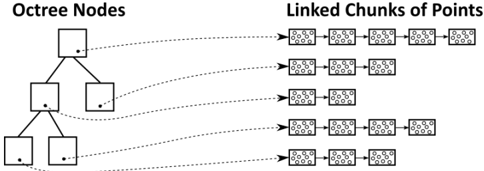
lists instead of grids - exactly the same as points. Figure 3 illustrates how more detailed, higher-level nodes are rendered close to the camera.
The difference to the structure of Schütz et al. [SKKW23] is that we store points and voxels in linked lists of chunks of points, which allows us to add additional capacity by allocating and linking additional chunks, as shown in Figure 4. An additional difference to Wand et al. [WBB*08] is that they use hash maps for their 128 3 voxel sampling grids, whereas we use a 128 3 bit = 256 kb occupancy grid per inner node to simplify massivelly parallel sampling on the GPU.
Despite the support for dynamic growth via linked lists, this structure still supports efficient rendering in compute-based pipelines, where each individual workgroup can process points in a chunk in parallel, and then traverse to the next chunk as needed. In our implementation, each chunk stores up to 1 , 000 points or voxels (Discussion in Section 7.4), with the latter being implemented as points where coordinates are quantized to the center of a voxel cell.
Figure 4: Octree nodes store 3D data as linked chunks of points/voxels. Linked chunks enable dynamic growth as new 3D data is added; efficient removal (after splitting leaves) by simply putting chunks back into a pool for re-use; and efficient rendering in compute-based pipelines.
<details>
<summary>Image 5 Details</summary>
### Visual Description
\n
## Diagram: Octree Node to Linked Chunk of Points Mapping
### Overview
The image is a diagram illustrating the relationship between Octree nodes and linked chunks of points. It depicts a binary tree structure (Octree) on the left, and a series of linked rectangular chunks containing points on the right. Dotted lines connect the Octree nodes to the corresponding chunks of points.
### Components/Axes
The diagram consists of two main sections:
* **Octree Nodes:** A binary tree structure representing the Octree. Each node is represented by a square.
* **Linked Chunks of Points:** A series of rectangular chunks, each containing a collection of points (represented by small circles). These chunks are linked together in a chain.
There are no explicit axes or scales in this diagram. The diagram is purely representational.
### Detailed Analysis or Content Details
The Octree consists of three levels.
* **Level 1:** A single root node.
* **Level 2:** Two child nodes branching from the root.
* **Level 3:** Four leaf nodes branching from the second-level nodes.
Each Octree node is connected to one or more chunks of points via dotted lines. The connections are as follows:
* The root node is connected to four chunks of points.
* The first second-level node is connected to two chunks of points.
* The second second-level node is connected to two chunks of points.
* The first third-level node is connected to one chunk of points.
* The second third-level node is connected to one chunk of points.
* The third third-level node is connected to one chunk of points.
* The fourth third-level node is connected to one chunk of points.
Each chunk of points contains approximately 10-15 points. The chunks are linked together, forming chains of varying lengths. The points within each chunk appear randomly distributed.
### Key Observations
* The diagram illustrates a hierarchical structure where each Octree node corresponds to a set of points.
* The number of chunks of points associated with each node varies.
* The chunks of points are linked, suggesting a spatial relationship between the points they contain.
* The diagram does not provide any quantitative data about the points or the Octree structure.
### Interpretation
This diagram likely represents a spatial partitioning data structure, specifically an Octree, used for efficient storage and retrieval of points in 3D space. The Octree recursively divides the space into eight octants, and each node in the tree represents a region of space. The linked chunks of points represent the actual point data stored within each region.
The connections between the Octree nodes and the chunks of points indicate that the points within a chunk belong to the corresponding region of space represented by the node. The linking of the chunks suggests that points in adjacent chunks may be spatially close to each other, allowing for efficient neighbor searches.
The varying number of chunks associated with each node could indicate that the point distribution is not uniform. Regions with a higher density of points may be subdivided into more chunks.
The diagram is a conceptual illustration and does not provide any specific details about the implementation or performance of the Octree. It serves to convey the basic idea of how an Octree can be used to organize and manage point data in 3D space.
</details>
## 3.2. Persistent Buffer
Since we require large amounts of memory allocations on the device from within the CUDA kernel throughout the LOD construction over hundreds of frames, we manage our own custom persistent buffer to keep the cost of memory allocation to a minimum. To that end, we simply pre-allocate 90% of the available GPU memory. An atomic offset counter keeps track of how much memory we already allocated and is used to compute the returned memory pointer during new allocations.
Note that sparse buffers via virtual memory management may be an alternative, as discussed in Section 8.
## 3.3. Voxel Sampling Grid
Voxels are sampled by inscribing a 128 3 voxel grid into each inner node, using 1 bit per cell to indicate whether that cell is still empty or already occupied. Inner nodes therefore require 256kb of memory in addition to the chunks storing the voxels (in our implementation as points with quantized coordinates). Grids are allocated from the persistent buffer whenever a leaf node is converted into an inner node.
## 3.4. Chunks and the Chunk Pool
We use chunks of points/voxels to dynamically increase the capacity of each node as needed, and a chunk pool where we return chunks that are freed after splitting a leaf node (chunk allocations for the newly created inner node are handled separately). Each chunk has a static capacity of N points/voxels (1 , 000 in our implementation), which makes it trivial to manage chunks as they all have the same size. Initially, the pool is empty and new chunks are allocated from the persistent buffer. When chunks are freed after splitting a leaf node, we store the pointers to these chunks inside the chunk pool. Future chunk allocations first attempt to acquire chunk pointers from the pool, and only allocate new chunks from the persistent buffer if there are none left in the pool.
## 4. Incremental LOD Construction - Overview
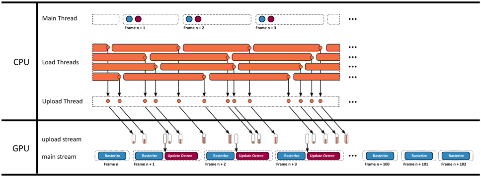
Our method loads batches of points from disk to GPU memory, updates the LOD structure in one CUDA kernel, and renders the updated results with another CUDA kernel. Figure 5
shows an overview of that pipeline. Both kernels utilize persistent threads [GSO12; KKSS18] using the cooperative group API [HP17] in order to merge numerous sub-passes into a single CUDA kernel. Points are loaded from disk to pinned CPU memory in batches of 1M points, utilizing multiple load threads. Whenever a batch is loaded, it is appended to a queue. A single uploader thread watches that queue and asynchronously copies any loaded batches to a queue in GPU memory. In each frame, the main thread launches the rasterize kernel that draws the entire scene, followed by an update kernel that incrementally inserts all batches of points into the octree that finished uploading to the GPU.
## 5. Incrementally Updating the Octree
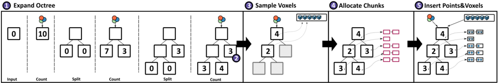
In each frame, the GPU may receive several batches of 1M points each. The update kernel loops through the batches and inserts them into the octree as shown in Figure 6. First, the octree is expanded until the resulting leaf nodes will hold at most 50k points. It then traverses each point of the batch through the octree again to generate voxels for inner nodes. Afterwards, it allocates sufficient chunks for each node to store all points in leaf-, and voxels in inner nodes. In the last step, it inserts the points and voxels into the newly allocated chunks of memory.
The premise of this approach is that it is cheaper in massively parallel settings to traverse the octree multiple times for each point and only insert them once at the end, rather than traversing the tree once per point but with the need for complex synchronization mechanisms whenever a node needs splitting or additional chunks of memory need to be allocated.
## 5.1. Expanding the Octree
CPU-based top-down approaches [WBB*08; SW11] typically traverse the hierarchy from root to leaf, update visited nodes along the way, and append points to leaf nodes. If a leaf node receives too many points, it 'spills" and is split into 8 child nodes. The points inside the spilling node are then redistributed to its newly generated child nodes. This approach works well on CPUs, where we can limit the insertion and expansion of a subtree to a single thread, but it raises issues in a massively parallel setting, where thousands of threads may want to insert points while we simultaneously need to split that node and redistribute the points it already contains.
To support massively parallel insertions of all points on the GPU, we propose an iterative approach that resembles a depthfirst-iterative-deepening search [Kor85]. Instead of attempting to fully expand the octree structure in a single step, we repeatedly expand it by one level until no more expansions are needed. This approach also decouples expansions of the hierarchy and insertions into a node's list of points, which is now deferred to a separate pass. Since we already defer the insertion of points into nodes, we also defer the redistribution of points from spilled nodes. We maintain a spill buffer, which accumulates points of spilled nodes. Points in the spill buffer are subsequently treated exactly the same as points inside the batch buffer that we are currently adding to the octree, i.e., the update kernel reinserts spilled points into the octree from scratch, along with the newly loaded batch of points.
## Timeline
<details>
<summary>Image 6 Details</summary>
### Visual Description
\n
## Diagram: CPU-GPU Frame Processing Pipeline
### Overview
The image depicts a diagram illustrating the flow of frame processing between the CPU and GPU. It shows how frames are processed through multiple threads on the CPU and then uploaded to the GPU for rasterization and octree updates. The diagram is structured as a timeline, showing the progression of frames (n+1, n+2, n+3, etc.).
### Components/Axes
The diagram is divided into two main sections: CPU and GPU. Within the CPU section, there are three thread types: Main Thread, Load Threads, and Upload Thread. The GPU section has two streams: upload stream and main stream. The horizontal axis represents time, with frames progressing from left to right.
### Detailed Analysis or Content Details
**CPU Section:**
* **Main Thread:** Displays a series of light blue rectangles labeled "Frame n+1", "Frame n+2", "Frame n+3", and so on, indicating the sequence of frames. Each frame has two orange circles above it.
* **Load Threads:** Multiple orange rectangles are stacked vertically, representing load threads. These threads appear to be working in parallel on different parts of the frame processing. The number of load threads is not explicitly stated, but there are approximately 8 visible.
* **Upload Thread:** A row of orange circles represents the upload thread. Each circle corresponds to a frame being uploaded to the GPU. Lines connect the upload thread to the load threads, indicating data transfer.
**GPU Section:**
* **Upload Stream:** Lines extend from the upload thread (CPU) to the upload stream (GPU).
* **Main Stream:** The main stream (GPU) consists of alternating light blue rectangles labeled "Rasterize" and light green rectangles labeled "Update Octree". These operations are performed on each frame. The frames are labeled "Frame n+1", "Frame n+2", "Frame n+3", "Frame n+100", "Frame n+101", "Frame n+102".
**Data Flow:**
1. The Main Thread initiates frame processing.
2. Load Threads perform processing tasks on the frame.
3. The Upload Thread transfers the processed frame data to the GPU.
4. The GPU's Upload Stream receives the data.
5. The GPU's Main Stream rasterizes and updates the octree for each frame.
### Key Observations
* The diagram highlights a parallel processing approach, with multiple load threads working concurrently on the CPU.
* The GPU performs alternating rasterization and octree update operations on each frame.
* The diagram shows a clear separation of tasks between the CPU and GPU.
* The number of load threads appears constant, while the number of frames processed is increasing.
* The diagram does not provide specific timing information or performance metrics.
### Interpretation
The diagram illustrates a typical CPU-GPU pipeline for rendering graphics. The CPU handles the initial frame processing and data preparation, while the GPU performs the computationally intensive tasks of rasterization and octree updates. The parallel processing on the CPU (Load Threads) suggests an attempt to optimize performance by utilizing multiple cores. The alternating rasterization and octree update operations on the GPU indicate a common rendering technique used in many graphics applications. The diagram suggests a system designed for continuous frame rendering, with a constant stream of frames being processed. The lack of specific timing information makes it difficult to assess the overall performance of the pipeline, but the diagram provides a clear overview of the data flow and processing steps involved. The diagram is a conceptual representation and does not provide concrete data points. It is a visual aid to understand the process rather than a quantitative analysis.
</details>
<details>
<summary>Image 7 Details</summary>

### Visual Description
Icon/Small Image (22x19)
</details>
<details>
<summary>Image 8 Details</summary>

### Visual Description
Icon/Small Image (32x22)
</details>
<details>
<summary>Image 9 Details</summary>

### Visual Description
Icon/Small Image (32x22)
</details>
<details>
<summary>Image 10 Details</summary>

### Visual Description
Icon/Small Image (30x19)
</details>
<details>
<summary>Image 11 Details</summary>

### Visual Description
Icon/Small Image (23x21)
</details>
<details>
<summary>Image 12 Details</summary>

### Visual Description
Icon/Small Image (22x23)
</details>
A batch of onemillionpoints.
Multiple load threads simultaneously load batches of points from the disk into pinned memory and queue them for upload.
Eachframe, the main thread launches the rasterization and update kernels.
- Therasterizationkernel renders the currentstateof the octree into an OpenGL framebuffer.
- The update kernel incrementally inserts all queued points into the octree.
Figure 5: Timeline of our system over several frames.
In detail, to expand the octree, we repeat the following two subpasses until no more nodes are spilled and all leaf nodes are marked as final for this update (see also Figure 6):
- Counting: In each iteration, we traverse the octree for each point of the batch and all spilled points accumulated in previous iterations during the current update, and atomically increment the point counter of each hit leaf node that is not yet marked as final by one.
- Splitting: All leaf nodes whose point counter exceeds a given threshold, e.g., 50k points, are split into 8 child nodes, each with a point counter of 0. The points it already contained are added to the list of spilled points. Note that the spilled points do not need to be associated with the nodes that they formerly belonged to - they are added to the octree from scratch. Furthermore, the chunks that stored the spilled points are released back to the chunk pool and may be acquired again later. Leaf nodes whose point counter does not exceed the threshold are marked as final so that further iterations during this update do not count points twice.
The expansion pass is finished when no more nodes are spilling, i.e., all leaf nodes are marked final.
## 5.2. Voxel Sampling
Lower levels of detail are populated with voxel representations of the points that traversed these nodes. Therefore, once the octree expansion is finished, we traverse each point through the octree again, and whenever a point visits an inner node, we project it into the inscribed 128 3 voxel sampling grid and check if the respective cell is empty or already occupied by a voxel. If the cell is empty, we create a voxel, increment the node's voxel counter, and set the corresponding bit in the sample grid to mark it as occupied. Note that in this way, the voxel gets the color of the first point that projects to it.
However, just like the points, we do not store voxels in the nodes right away because we do not know the amount of memory/chunks that each node requires until all voxels for the current incremental update are generated. Thus, voxels are first stored in a temporary backlog buffer with a large capacity. In theory, adding a batch of 1 million points may produce up to ( octreeLevels -1 ) million voxels because each inner node's sampling grid has the potential to hold 128 3 = 2 M voxels, and adding spatially close points may lead to several new octree levels until they are all separated into leaf nodes with at most 50k points. However, in practice, none of the test data sets of this paper produced more than 1M voxels per batch of 1M points, and of our numerous other data sets, the largest required backlog size was 2.4M voxels. Thus, we suggest using a backlog size of 10M points to be safe.
## 5.3. Allocating Chunks
After expansion and voxel sampling, we now know the exact amount of points and voxels that we need to store in leaf and inner nodes. Using this knowledge, we check all affected nodes whether their chunks have sufficient free space to store the new points/voxels, or if we need to allocate new chunks of memory to raise the nodes' capacity by 1000 points or voxels per chunk. In total, we need ⌊ counter + POINTS \_ PER \_ CHUNK -1 POINTS \_ PER \_ CHUNK ⌋ linked chunks per node.
(a) Adding 10 points to the octree. (1) Expanding the octree by repeatedly counting and splitting until leaf nodes hold at most T points (depicted: 5, in practice: 50k). (2) Leaves that were not split do not count points again. (3) The voxel sampling pass inserts all points again, creates voxels for empty cells in inner nodes, and stores new voxels (and the nodes they belong to) in a temporary backlog buffer. (4) Now that we know the number of new points and voxels, we allocate the necessary chunks (depicted size: 2, in practice: 1000) to store them. (5) All points are inserted again, traverse to the leaf, and are inserted into the chunks. Voxels from the backlog are inserted into the respective inner nodes.
<details>
<summary>Image 13 Details</summary>
### Visual Description
\n
## Diagram: Octree Processing Pipeline
### Overview
The image depicts a four-stage pipeline for processing an octree data structure. The stages are: Expand Octree, Sample Voxels, Allocate Chunks, and Insert Points & Voxels. Each stage visually demonstrates the transformation of data within the octree, with numerical values indicating counts or identifiers. The diagram uses a series of boxes representing octree nodes, arrows indicating data flow, and color-coded icons to represent different data types.
### Components/Axes
The diagram is divided into four columns, each representing a stage in the pipeline. Each column has a header indicating the stage name (1. Expand Octree, 2. Sample Voxels, 3. Allocate Chunks, 4. Insert Points & Voxels). Below each header is a visual representation of the octree structure at that stage. The bottom of each column has labels: "Input", "Count", "Split", and "Count". There are also icons at the top of each column representing data types. The icons are: a sphere, a cube, and a collection of smaller cubes.
### Detailed Analysis or Content Details
**Stage 1: Expand Octree**
* **Input:** A single box labeled "0" with the value "10" below it.
* **Split:** The initial box splits into eight smaller boxes. The values within these boxes are: 0, 0, 7, 3, 3, 0, 0, 3.
* **Count:** The final "Count" box shows the value "10".
**Stage 2: Sample Voxels**
* **Input:** The octree structure from Stage 1.
* **Sample Voxels:** Several boxes are shaded gray, indicating they are being sampled. The values within the remaining boxes are: 4, 3, 2, 4.
* **Count:** The final "Count" box shows the value "4".
**Stage 3: Allocate Chunks**
* **Input:** The octree structure from Stage 2.
* **Allocate Chunks:** Pink rectangles are connected to the octree nodes with arrows, representing chunk allocation. The values within the boxes are: 4, 2, 3, 4.
* **Count:** The final "Count" box shows the value "4".
**Stage 4: Insert Points & Voxels**
* **Input:** The octree structure from Stage 3.
* **Insert Points & Voxels:** The octree nodes now contain additional data represented by small, colored squares. The values within the boxes are: 4, 2, 3, 4.
* **Count:** The final "Count" box shows the value "4".
### Key Observations
* The "Count" value decreases from 10 in the first stage to 4 in the final stage. This suggests a reduction in the number of elements being processed.
* The graying out of boxes in Stage 2 indicates a sampling process, potentially filtering or selecting specific voxels.
* The pink rectangles in Stage 3 represent the allocation of chunks, likely for memory management or parallel processing.
* The addition of colored squares in Stage 4 indicates the insertion of points and voxels into the octree structure.
### Interpretation
This diagram illustrates a pipeline for processing octree data, likely for representing 3D space or volumetric data. The pipeline begins by expanding an initial octree node (0) into its eight children. The "Count" value represents the total number of elements within the octree. The subsequent stages involve sampling voxels, allocating chunks, and inserting points and voxels, ultimately resulting in a refined octree structure. The reduction in the "Count" value suggests that the sampling process filters out some voxels, while the chunk allocation and point insertion stages prepare the data for further processing or rendering. The diagram demonstrates a common approach to managing and processing large 3D datasets efficiently. The icons at the top of each stage suggest the data types being handled: a sphere (likely representing a point), a cube (representing a voxel), and a collection of smaller cubes (representing the octree structure itself).
</details>
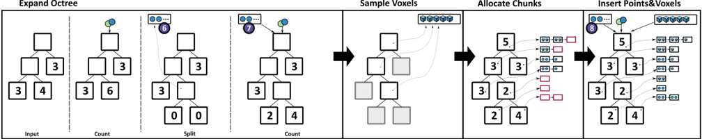
(b) For illustrative purposes, we now add a batch of just two points which makes one of the nodes spill. (6) When splitting, we move all previously inserted points into a spill buffer. (7, 8) for the remainder of this frame's update, points in the spill buffer and the current batch get identical treatment.
<details>
<summary>Image 14 Details</summary>
### Visual Description
## Diagram: Octree Processing Pipeline
### Overview
This diagram illustrates a four-stage pipeline for processing data using an Octree structure. The stages are: Expand Octree, Sample Voxels, Allocate Chunks, and Insert Points & Voxels. The diagram shows the data flow and transformations at each stage, with numerical values indicating counts or allocations within the Octree nodes.
### Components/Axes
The diagram is divided into four columns, each representing a stage in the pipeline. Each column has a title indicating the stage's function. Within each stage, there are Octree structures represented as nested squares, with numbers inside indicating counts. Arrows show the flow of data between stages. There are also visual representations of data structures (arrays of squares) at the top of each stage, representing input or output. The bottom of each stage has labels: "Input", "Count", "Split", and "Count".
### Detailed Analysis or Content Details
**Stage 1: Expand Octree**
* **Input:** An initial Octree structure is shown.
* **Count:** The root node has a count of 3. The four child nodes each have a count of 3, 4, 3, and 6 respectively.
* **Split:** The Octree is shown splitting into its child nodes.
* **Count:** The child nodes have counts of 0, 0, 2, and 4 respectively.
* A blue sphere with a number "6" above it is connected to the root node.
**Stage 2: Sample Voxels**
* An array of six grey squares is shown at the top, representing sampled voxels.
* The Octree structure is similar to the "Split" stage of the previous step, with counts of 3, 3, 3, and 3.
* The bottom row shows counts of 0, 0, 2, and 4.
* A blue sphere with a number "7" above it is connected to the root node.
**Stage 3: Allocate Chunks**
* An array of six grey squares is shown at the top, representing allocated chunks.
* The Octree structure is shown with counts of 5, 3, 3, and 2.
* The bottom row shows counts of 3, 2, 4, and 0.
* Pink rectangles are connected to the nodes with counts of 5, 3, 3, and 2.
* A blue sphere with a number "9" above it is connected to the root node.
**Stage 4: Insert Points & Voxels**
* An array of six grey squares is shown at the top, representing inserted points and voxels.
* The Octree structure is shown with counts of 5, 3, 3, and 2.
* The bottom row shows counts of 2, 4, 0, and 0.
* Pink rectangles are connected to the nodes with counts of 5, 3, 3, and 2.
* A blue sphere with a number "12" above it is connected to the root node.
The arrows indicate a flow from left to right, showing how the Octree is expanded, sampled, chunks are allocated, and finally, points and voxels are inserted.
### Key Observations
* The counts within the Octree nodes change at each stage, reflecting the processing steps.
* The blue spheres above the root nodes have increasing numbers (6, 7, 9, 12), potentially representing a cumulative count or a stage identifier.
* The pink rectangles appear in the "Allocate Chunks" and "Insert Points & Voxels" stages, suggesting they represent allocated memory or data associated with those stages.
* The counts at the bottom of each stage seem to represent the number of elements at the leaf nodes of the Octree.
### Interpretation
This diagram demonstrates a hierarchical data processing pipeline using an Octree. The Octree is used to subdivide space, and the pipeline stages operate on these subdivisions. The "Expand Octree" stage initializes the structure. "Sample Voxels" selects data points within the Octree. "Allocate Chunks" assigns memory or resources to the Octree nodes. Finally, "Insert Points & Voxels" populates the Octree with data. The increasing numbers on the blue spheres could represent the total number of points/voxels processed up to that stage. The pink rectangles likely represent allocated memory or data structures associated with the chunks. The diagram suggests an efficient way to manage and process spatial data by leveraging the hierarchical structure of the Octree. The decreasing counts at the bottom of the stages could indicate a refinement or filtering process as data moves through the pipeline.
</details>
Figure 6: The CUDA kernel that incrementally updates the octree. (a) First, it inserts a batch with 10 points into the initially empty octree and (b) then adds another batch with two points that causes a split of a non-empty leaf node.
## 5.4. Storing Points and Voxels
To store points inside nodes, we traverse each point from the input batch and the spill buffer again through the octree to the respective leaf node and atomically update that node's numPoints variable. The atomic update returns the point index within the node, from which we can compute the index of the chunk and the index within the chunk where we store the point.
We then iterate through the voxels in the backlog buffer, which stores voxels and for each voxel a pointer to the inner node that it belongs to. Insertion is handled the same way as points - we atomically update each node's numVoxels variable, which returns an index from which we can compute the target chunk index and the position within that chunk.
## 6. Rendering
Points and voxels are both drawn as pixel-sized splats by a CUDA kernel that utilizes atomic operations to retain the closest sample in each pixel [GKLR13; Eva15; SKW22]. Custom computebased software-rasterization pipelines are particularly useful for our method because traditional vertex-shader-based pipelines are not suitable for drawing linked lists of chunks of points. A CUDA kernel, however, has no issues looping through points in a chunk, and then traversing to the next chunk in the list. The recently introduced mesh and task shaders could theoretically also deal with linked lists of chunks of points, but they may benefit from smaller chunk sizes, and perhaps even finer-grained nodes (smaller sam- pling grids that lead to fewer voxels per node, and a lower maximum of points in leaf nodes).
During rendering, we first assemble a list of visible nodes, comprising all nodes whose bounding box intersects the view frustum and which have a certain size on screen. Since inner nodes have a voxel resolution of 128 3 , we need to draw their half-sized children if they grow larger than 128 pixels. We draw nodes that fulfill the following conditions:
- Nodes that intersect the view frustum.
- Nodes whose parents are larger than 128 pixels. In that case, the parent is hidden and all its children are made visible instead.
Figure 3 illustrates the resulting selection of rendered octree nodes within a frustum. Seemingly higher-LOD nodes are rendered towards the edge of the screen due to perspective distortions that make the screen-space bounding boxes bigger. For performancesensitive applications, developers may instead want to do the opposite and reduce the LOD at the periphery and fill the resulting holes by increasing the point sizes.
To draw points or voxels, we launch one workgroup per visible node whose threads loop through all samples of the node and jump to the next chunk when needed, as shown in listing 1.
```
for (int i = 0; i < nodes[workgroupIndex].points.size(); i++) {
if (nodes[workgroupIndex].points.get(i).isSmaller) {
pointIndex = i;
break;
}
}
```
```
```
Listing 1: CUDA code showing threads of a workgroup iterating through all points in a node, processing num\_threads points at a time in parallel. Threads advance to the next chunk as needed.
## 7. Evaluation
Our method was implemented in C++ and CUDA, and evaluated on the test data sets shown in Figure 7.
The following systems were used for the evaluation:
| OS | GPU | CPU | Disk |
|------------|----------|---------------|-----------------|
| Windows 10 | RTX 3060 | Ryzen 7 2700X | Samsung 980 PRO |
| Windows 11 | RTX 4090 | Ryzen 9 7950X | Crucial T700 |
Special care was taken to ensure meaningful results for disk IO in our benchmarks:
- On Microsoft Windows, traditional C++ file IO operations such as fread or ifstream are automatically buffered by the operating system. This leads to two issues - First, it makes the initial access to a file slower and significantly increases CPU usage, which decreases the overall performance of the application and caused stutters when streaming a file from SSD to GPU for the first time. Second, it makes future accesses to the same file faster because the OS now serves it from RAM instead of reading from disk.
- Since we are mostly interested in first-read performance, we implemented file access on Windows via the Windows API's ReadFileEx function together with the FILE\_FLAG\_NO\_BUFFERING flag. It ensures that data is read from disk and also avoids caching it in the first place. As an added benefit, it also reduces CPU usage and resulting stutters.
We evaluated the following performance aspects, with respect to our goal of simultaneously updating the LOD structure and rendering the intermediate results:
1. Throughput of the incremental LOD construction in isolation.
2. Throughput of the incremental LOD construction while streaming points from disk and simultaneously rendering the interme-
2. diate results in real time.
3. Average and maximum duration of all incremental updates.
4. Performance of rendering nodes up to a certain level of detail.
## 7.1. Data Sets
We evaluated a total of five data sets shown in Figure 7, three file formats, and Morton-ordering vs. the original ordering by scan position. Chiller and Meroe are photogrammetry-based data sets, Morro Bay is captured via aerial LIDAR, Endeavor via terrestrial laser scans, and Retz via a combination of terrestrial (town center, high-density) and aerial LIDAR (surrounding, low-density).
The LAS and LAZ file formats are industry-standard point cloud formats. Both store XYZ, RGB, and several other attributes. Due to this, LAS requires either 26 or 34 bytes per point for our data sets. LAZ provides a good and lossless compression down to around 2-5 bytes/point, which is why most massive LIDAR data sets are distributed in that format. However, it is quite CPU-intensive and therefore slow to decode. SIM is a custom file format that stores points in the update kernel's expected format - XYZRGBA (3 x float + 4 x uint8, 16 bytes per point).
Endeavor is originally ordered by scan position and the timestamp of the points, but we also created a Morton-ordered variation to evaluate the impact of the order.
## 7.2. Construction Performance
Table 1 covers items 1-3 and shows the construction performance of our method on the test systems. The incremental LOD construction kernel itself achieves throughputs of up to 300M points per second on an RTX 3060, and up to 1.2 billion points per second on an RTX 4090. The whole system, including times to stream points from disk and render intermediate results, achieves up to 100 million points per second on an RTX 3060 and up to 580 million points per second on the RTX 4090. The durations of the incremental updates are indicators for the overall impact on fps (average) and occasional stutters (maximum). We implemented a time budget of 10ms per frame to reduce the maximum durations of the update kernel (RTX 3060: 45ms → 16ms; RTX 4090 25ms → 13ms). After the budget is exceeded, the kernel stops and resumes the next frame. Our method benefits from locality as shown by the Morton-ordered variant of the Endeavor data set, which increases the construction performance by a factor of x2.5 (497 MP/s → 1221 MP/s).
## 7.3. Rendering Performance
Regarding rendering performance, we show that linked lists of chunks of points/voxels are suitable for high-performance real-time rendering by rendering the constructed LOD structure at high resolutions (pixel-sized voxels), whereas performance-sensitive rendering engines (targeting browsers, VR, ...) would limit the number of points/voxels of the same structure to a point budget in the singledigit millions, and then fill resulting gaps by increasing point sizes accordingly. Table 3 shows that we are able to render up to 89.4 million pixel-sized points and voxels in 2.7 milliseconds, which leaves the majority of a frame's time for the construction kernel (or higher-quality shading). Table 4 shows that the size of chunks has negligible impact on rendering performance (provided they are larger than the workgroup size).
We implemented the atomic-based point rasterization by Schütz et al. [SKW21], including the early-depth test. Compared to their
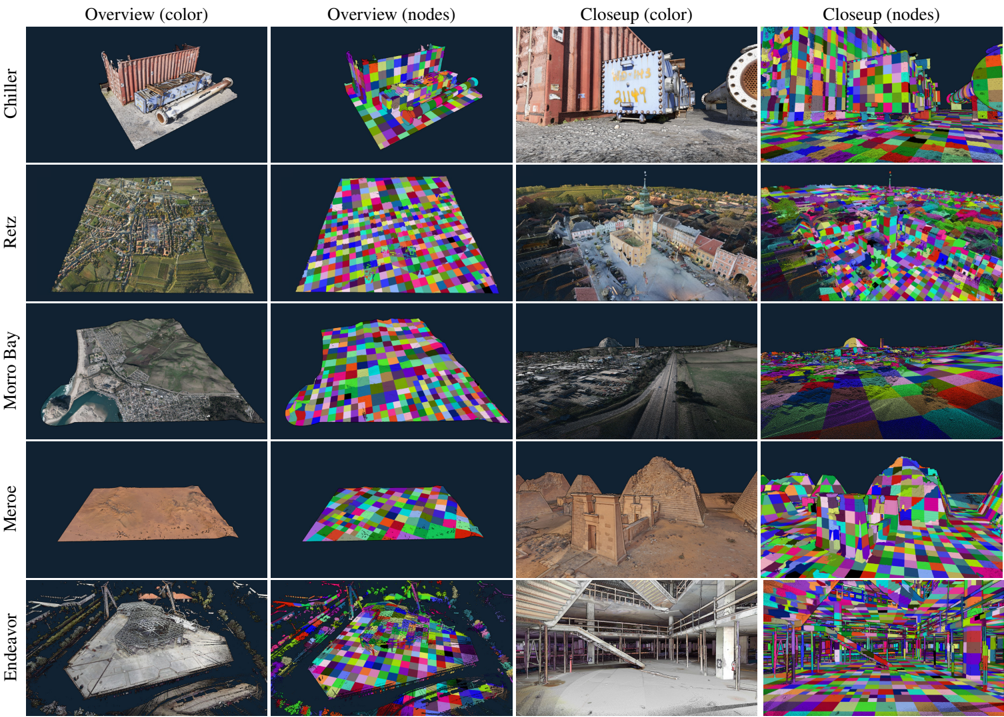
Figure 7: Overview and close-ups of our test data sets. The second and fourth columns illustrate the rendered octree nodes.
<details>
<summary>Image 15 Details</summary>
### Visual Description
\n
## Image Analysis: Urban Environment Visualizations
### Overview
The image presents a comparative visualization of five different urban environments – Chiller, Retz, Morro Bay, Meroe, and Endeavor. Each environment is depicted in four views: an overview showing colorized representation, an overview showing a node-based representation, a closeup showing colorized representation, and a closeup showing a node-based representation. The visualizations appear to be derived from 3D scans or models of these locations.
### Components/Axes
The image is organized as a 5x4 grid.
* **Rows:** Represent the different urban environments (Chiller, Retz, Morro Bay, Meroe, Endeavor).
* **Columns:** Represent the different visualization types:
* Overview (color)
* Overview (nodes)
* Closeup (color)
* Closeup (nodes)
There are no explicit axes or scales present. The "color" views appear to be a rendering of the 3D model with color applied, while the "nodes" views represent the environment as a grid of colored squares, potentially representing data points or features.
### Detailed Analysis or Content Details
**Chiller:**
* Overview (color): Shows a building interior, possibly a warehouse or industrial space, with a white structure and dark flooring.
* Overview (nodes): A grid of colored squares (red, yellow, green, blue, purple) covering a rectangular area.
* Closeup (color): A shipping container with graffiti on it. The graffiti includes yellow and blue paint.
* Closeup (nodes): A grid of colored squares (red, yellow, green, blue, purple) covering a smaller rectangular area.
**Retz:**
* Overview (color): Shows a dense urban area with buildings and streets.
* Overview (nodes): A grid of colored squares (red, yellow, green, blue, purple) covering a rectangular area.
* Closeup (color): A building facade with a dark-colored wall and a door.
* Closeup (nodes): A grid of colored squares (red, yellow, green, blue, purple) covering a smaller rectangular area.
**Morro Bay:**
* Overview (color): Shows a coastal landscape with a large rock formation (Morro Rock) and a shoreline.
* Overview (nodes): A grid of colored squares (red, yellow, green, blue, purple) covering a rectangular area.
* Closeup (color): A railway track with a building in the background.
* Closeup (nodes): A grid of colored squares (red, yellow, green, blue, purple) covering a smaller rectangular area.
**Meroe:**
* Overview (color): Shows a desert landscape with pyramid-like structures.
* Overview (nodes): A grid of colored squares (red, yellow, green, blue, purple) covering a rectangular area.
* Closeup (color): A pyramid-like structure with a textured surface.
* Closeup (nodes): A grid of colored squares (red, yellow, green, blue, purple) covering a smaller rectangular area.
**Endeavor:**
* Overview (color): Shows a large, open interior space, possibly a factory or warehouse, with a complex roof structure.
* Overview (nodes): A grid of colored squares (red, yellow, green, blue, purple) covering a rectangular area.
* Closeup (color): An interior view of the same space, showing support beams and a concrete floor.
* Closeup (nodes): A grid of colored squares (red, yellow, green, blue, purple) covering a smaller rectangular area.
The node-based views consistently use the colors red, yellow, green, blue, and purple, distributed seemingly randomly across the grid. The density of nodes appears relatively uniform across all environments.
### Key Observations
* The "nodes" visualizations consistently use the same color palette across all environments.
* The "color" visualizations show a diverse range of environments, from indoor industrial spaces to outdoor urban and natural landscapes.
* The "closeup" views provide more detailed representations of specific features within each environment.
* There is no quantitative data presented; the image is purely visual.
### Interpretation
The image likely demonstrates a method for visualizing and analyzing urban environments using 3D scanning or modeling techniques. The "color" views provide a realistic representation of the environment, while the "nodes" views may represent a data layer overlaid on the environment, potentially indicating points of interest, sensor locations, or other relevant data. The consistent use of the same color palette in the "nodes" views suggests that the colors may represent different categories or values of data.
The purpose of this visualization could be for urban planning, environmental monitoring, or security applications. The node-based representation could be used to identify patterns, anomalies, or areas of concern within the environment. The comparison of different environments allows for a visual assessment of their characteristics and potential challenges.
The image does not provide enough information to determine the specific meaning of the colors or the data represented by the nodes. Further context would be needed to fully understand the purpose and implications of these visualizations. The image is a demonstration of a visualization technique, rather than a presentation of specific data findings.
</details>
brute-force approach that renders all points in each frame, our onthe-fly LOD approach reduces rendering times on the RTX 4090 by about 5 to 12 times, e.g. Morro Bay is rendered about 5 to 9 times faster (overview: 7.1ms → 0.8ms; closeup: 6.3ms → 1.1ms) and Endeavor is rendered about 5 to 12 times faster (overview: 13.7ms → 1.1ms; closeup: 13.8ms → 2.7ms). Furthermore, the generated LOD structures would allow improving rendering performance even further by lowering the detail to less than 1 point per pixel. In terms of throughput (rendered points/voxels per second), our method is several times slower (Morro Bay overview: 50MP/s → 15.8MP/s; Endeavor overview: 58MP/s → 15.5MP/s). This is likely because throughput dramatically rises with overdraw, i.e., if thousands of points project to the same pixel, they share state and collaboratively update the pixel.
At this time, we did not implement the approach presented in Schütz et al.'s follow-up paper [SKW22] that further improves rendering performance by compressing points and reducing memory bandwidth.
## 7.4. Chunk Sizes
Table 4 shows the impact of chunk sizes on LOD construction and rendering performance. Smaller chunk sizes reduce memory usage but also increase construction duration. The rendering duration, on the other hand, is largely unaffected by the range of tested chunk sizes. We opted for a chunk size of 1k for this paper because it makes our largest data set Endeavor - fit on the GPU, and because the slightly better construction kernel performance of larger chunks did not significantly improve the total throughput of the system.
## 7.5. Performance Discussion
Our approach constructs LOD structures up to 320 times faster than the incremental, CPU-based approach of Bormann et al. [BDSF22] (1.8MP/s → 580MP/s) (Peak result of 1.8MP/s taken from Bormann et al.) while points are simultaneously rendered on the same GPU, and up to 677 times faster if we only account for the construction times (1.8MP/s → 1222MP/s). On the same 4090 test system, our incremental approach is about 7.6 times slower than the non-incremental, GPU-based construction method of Schütz et al. [SKKW23] for the same first-come sampling method (Morro
M. Schütz & L. Herzberger & M. Wimmer / SimLOD: Simultaneous LOD Generation and Rendering 9 of 12
| Data Set | GPU | points | | | Update | Update | Duration | Duration | Throughput | Throughput | Throughput |
|--------------------|----------|----------|--------|-----------|----------|----------|---------------|-------------|----------------|--------------|--------------|
| Data Set | GPU | (M) | format | size (GB) | avg (ms) | max (ms) | updates (sec) | total (sec) | updates (MP/s) | total (MP/s) | total (GB/s) |
| Chiller | RTX 3060 | 73.6 | LAS | 1.9 | 1.2 | 13.3 | 0.2 | 1.3 | 297 | 54 | 1.4 |
| | | | SIM | 1.2 | 2.0 | 14.0 | 0.2 | 0.8 | 298 | 87 | 1.4 |
| Retz | | 145.5 | LAS | 4.9 | 1.0 | 14.9 | 0.6 | 3.2 | 260 | 45 | 1.5 |
| | | | SIM | 2.3 | 2.8 | 14.3 | 0.5 | 1.6 | 272 | 91 | 1.4 |
| Morro Bay | | 350.0 | LAS | 11.9 | 1.2 | 15.9 | 1.4 | 7.6 | 242 | 46 | 1.6 |
| | | | SIM | 5.6 | 4.1 | 16.1 | 1.4 | 3.5 | 247 | 100 | 1.6 |
| Chiller | RTX 4090 | 73.6 | LAS | 1.9 | 0.6 | 7.5 | 0.1 | 0.3 | 1,215 | 291 | 7.5 |
| | | | SIM | 1.2 | 0.6 | 8.0 | 0.1 | 0.2 | 1,217 | 439 | 7.2 |
| Retz | | 145.5 | LAS | 4.9 | 0.4 | 8.0 | 0.1 | 0.7 | 1,145 | 221 | 7.4 |
| | | | SIM | 2.3 | 1.0 | 8.6 | 0.1 | 0.4 | 1,187 | 425 | 6.7 |
| Morro Bay | | 350.0 | LAS | 11.9 | 0.6 | 9.2 | 0.4 | 1.5 | 979 | 234 | 8.0 |
| | | | SIM | 5.6 | 1.5 | 10.9 | 0.3 | 0.8 | 1,030 | 458 | 7.3 |
| Meroe | | 684.4 | LAS | 23.3 | 0.7 | 10.4 | 0.8 | 2.8 | 882 | 241 | 8.2 |
| | | | SIM | 11.4 | 1.9 | 12.1 | 0.7 | 1.7 | 945 | 401 | 6.4 |
| Endeavor | | 796.0 | LAS | 20.7 | 7.0 | 12.6 | 1.6 | 2.6 | 497 | 307 | 8.0 |
| | | | LAZ | 8.0 | 0.2 | 7.2 | 2.4 | 25.1 | 328 | 32 | 0.3 |
| | | | SIM | 12.7 | 9.1 | 12.9 | 1.6 | 2.3 | 497 | 341 | 5.4 |
| Endeavor (z-order) | | | SIM | 12.7 | 2.2 | 10.7 | 0.7 | 1.4 | 1,221 | 581 | 9.3 |
Table 1: LOD Construction Performance showing average and maximum durations of the update kernel, total duration of all updates or the whole system, and the throughput in million points per second (MP/s) or gigabytes per second (GB/s). Total duration includes the time to load points from disk, stream them to the GPU, and insert them into the octree. Update measures the duration of all incremental per-frame (may process multiple batches) updates in isolation. Throughput in GB/s refers to the file size, which depends on the number of points and the storage format (ranging from 10 (LAZ), 16(SIM) to 26 or 34(LAS) byte per point).
| | overview | overview | overview | overview | closeup | closeup | closeup | closeup |
|-----------|------------|------------|------------|------------|-----------|-----------|-----------|-----------|
| | points | voxels | nodes | duration | points | voxels | nodes | duration |
| Chiller | 1.5M | 10.3M | 450 | 1.3 ms | 22.7M | 19.5M | 1813 | 3.5 ms |
| Morro Bay | 0.4M | 12.5M | 518 | 1.5 ms | 8.8M | 16.2M | 1065 | 2.2 ms |
| Meroe | 1.4M | 2.5M | 208 | 0.9 ms | 24.6M | 21.0M | 2069 | 3.7 ms |
| Endeavor | 5.2M | 11.8M | 914 | 2.1 ms | 54.0M | 50.7M | 4811 | 7.5 ms |
Table 2: Rendering performance from overview and closeup viewpoints shown in Figure 7. Points and voxels are both rendered as pixel-sized splats. Some voxels may be processed but discarded because they are replaced by higher-res data in visible child nodes. Up to 104 million points+voxels stored in linked-lists inside 4 , 811 octree nodes are rasterized at >120fps for close-up views at high levels of detail.
| | | overview | overview | overview | overview | overview | closeup | closeup | closeup | closeup | closeup |
|-----------|------|------------|------------|------------|------------|------------|-----------|-----------|-----------|-----------|------------|
| | GPU | points | voxels | nodes | duration | samples/ms | points | voxels | nodes | duration | samples/ms |
| Chiller | 3060 | 2.6M | 8.4M | 441 | 3.3 ms | 3.3M | 28.0M | 7.9M | 1678 | 7.4 ms | 4.9M |
| Retz | | 5.2M | 12.4M | 644 | 4.4 ms | 4.0M | 18.9M | 7.5M | 1616 | 6.0 ms | 4.4M |
| Morro Bay | | 0.6M | 12.0M | 477 | 3.5 ms | 3.6M | 16.3M | 13.7M | 1346 | 6.5 ms | 4.6M |
| Chiller | 4090 | 2.6M | 8.4M | 441 | 0.7 ms | 15.7M | 28.0M | 7.9M | 1678 | 1.3 ms | 27.6M |
| Retz | | 5.2M | 12.4M | 644 | 0.8 ms | 22.0M | 18.9M | 7.5M | 1616 | 1.1 ms | 24.0M |
| Morro Bay | | 0.6M | 12.0M | 477 | 0.8 ms | 15.8M | 16.3M | 13.7M | 1346 | 1.1 ms | 27.3M |
| Meroe | | 1.9M | 2.0M | 190 | 0.5 ms | 7.8M | 36.4M | 17.5M | 2500 | 1.9 ms | 28.4M |
| Endeavor | | 6.5M | 10.5M | 906 | 1.1 ms | 15.5M | 72.7M | 16.7M | 4956 | 2.7 ms | 33.1M |
Table 3: Rendering performance from overview and closeup viewpoints shown in Figure 7. Samples (Points+Voxels) are both rendered as pixel-sized splats.
| Chunk Size | construct (ms) | Memory (GB) | rendering (ms) |
|--------------|------------------|---------------|------------------|
| 500 | 933.9 | 17.1 | 1.9 |
| 1 000 | 734.9 | 17.2 | 1.9 |
| 2 000 | 654.5 | 17.6 | 1.9 |
| 5 000 | 618.1 | 18.9 | 1.9 |
| 10 000 | 611 | 21 | 1.9 |
Table 4: The Impact of points/voxels per chunk on total construction duration, memory usage for octree data, and rendering times. (Close-up viewpoint of the Meroe data set on an RTX 4090)
Bay: 7500 MP/s → 979 MP/s), but about 18 times (Morro Bay; LAS; with rendering: 13 MP/s → 234 MP/s) to 75 times (Morro Bay; LAS; construction: 13 MP/s → 979 MP/s) faster than their non-incremental, CPU-based method [SOW20].
In practice, point clouds are often compressed and distributed as LAZ files. LAZ compression is lossless and effective, but slow to decode. Incremental methods such as Bormann et al. [BDSF22] and ours are especially interesting for these as they allow users to immediately see results while loading is in progress. Although nonincremental methods such as [SKKW23] feature a significantly higher throughput of several billions of points per second, they are nevertheless bottle-necked by the 32 million points per second (see Table 1, Endeavor) with which we can load and decompress such data sets, while they can only display the results after loading and processing is fully finished.
## 8. Conclusion, Discussion and Potential Improvements
In this paper, we have shown that GPU-based computing allows us to incrementally construct an LOD structure for point clouds at the rate at which points can be loaded from an SSD, and immediately display the results to the user in real time. Thus, users are able to quickly inspect large data sets right away. without the need to wait until LOD construction is finished.
There are, however, several limitations and potential improvements that we would like to mention:
- Out-of-Core : This approach is currently in-core only and serves as a baseline and a step towards future out-of-core approaches. For arbitrarily large data sets, out-of-core approaches are necessary that flush least-recently-modified-and-viewed nodes to disk. Once they are needed again, they will have to be reloaded - either because the node becomes visible after camera movement, or because newly loaded points are inserted into previously flushed nodes.
- Compression : In-between 'keeping the node's growable data structure in memory" and 'flushing the entire node to disk" is the potential to keep nodes in memory, but convert them into a more efficient structure. 'Least recently modified" nodes can be converted into a non-growable, compressed form with higher memory and rendering efficiency, and 'least recently modified and viewed" nodes could be compressed even further and decoded on-demand for rendering. For reference, voxel coordinates could be encoded relative to voxels in parent nodes, which requires about 2 bit per voxel, and color values of z-ordered voxels could
be encoded with BC texture compression [BC], which requires about 8 bit per color, for a total of 10 bit per voxel. Currently, our implementation uses 16 bytes (128 bit) per voxel.
- Color-Filtering : Our implementation currently does a firstcome color sampling for voxels, which leads to aliasing artifacts similar to textured meshes without mipmapping, or in some cases even bias towards the first scan in a collection of multiple overlapping scans. The implementation offers a rendering mode that blends overlapping points [BHZK05; SKW21], which significantly improves quality, but a sparse amount of overlapping points at low LODs are not sufficient to reconstruct a perfect representation of all the missing points from higher LODs. Thus, proper color filtering approaches will need to be implemented to create representative averages at lower levels of detail. We implemented averaging in post-processing [SKKW23], but in the future, we would like to integrate color sampling directly into the incremental LOD generation pipeline. The main reason we did not do this yet is the large amount of extra memory that is required to accumulate colors for each voxel, rather than the single bit that is required to select the first color. We expect that this approach can work with the help of least-recently-used queues that help us predict which nodes still need high-quality sampling grids, and which nodes do not need them anymore. This can also be combined with the hash map approach by Wand et al. [WBB*08], which reduces the amount of memory of each individual sampling grid.
- Quality : To improve quality, future work in fast and incremental LOD construction may benefit from fitting higher quality point primitives (Surfels, Gaussian Splats, ... [PZvBG00; ZPvBG01; WHA*07;KKLD23]) to represent lower levels of detail. Considering the throughput of SSDs (up to 580M Points/sec), efficient heuristics to quickly generate and update splats are required, and load balancing schemes that progressively refine the splats closer to the user's current viewpoint.
- Sparse Buffers : An alternative to the linked-list approach for growable arrays of points may be the use of virtual memory management (VMM) [PS20]. VMM allows allocating large amounts of virtual memory, and only allocates actual physical memory as needed (similar to OpenGL's ARB\_sparse\_buffer extension [Inc14]). Thus, each node could allocate a massive virtual capacity for its points in advance, progressively back it with physical memory as the amount of points we add grows, and thereby make linked lists obsolete. We did not explore this option at this time because our entire update kernel - including allocation of new nodes, insertion of points and required allocations of additional memory, etc. - runs on the device, while VMMoperations must be called from the host.
The source code for this paper is available at https:// github.com/m-schuetz/SimLOD . The repository also contains several subsets of the Morro Bay data set (which in turn is a subset of San Simeon [CA13]) in different file formats.
## 9. Acknowledgements
The authors wish to thank Weiss AG for the Chiller data set; Riegl Laser Measurement Systems for providing the data set of the town of Retz ; PG&E and Open Topography for the Morro Bay data set (a
subset of the San Simeon data set) [CA13]; Iconem for the Northern necropolis - Meroë data set [Meroe]; NVIDIA for the Endeavor data set; Keenan Crane for the Spot model; and Bunds et al. [CA19] for the San Andras Fault data set.
This research has been funded by WWTF project ICT22-055 Instant Visualization and Interaction for Large Point Clouds , and FFG project LargeClouds2BIM .
## References
- [3DEP] 3D Elevation Program (3DEP) . https://www.usgs.gov/ core-science-systems/ngp/3dep , Accessed 2020.09.18 2.
- [AHN] AHN . https : / / www . ahn . nl / kwaliteitsbeschrijving , Accessed 2023.06.01 2.
- [AHN2] AHN2 . https : / / www . pdok . nl / introductie/ /article/actueel-hoogtebestand-nederland-ahn2-, Accessed 2021.03.27 2.
- [BC] MICROSOFT. BC7 Format . Accessed 2023.06.09. 2022. URL: https : / / learn . microsoft . com / en -us / windows / win32 / direct3d11 / bc7 - format # bc7 implementation/ 10.
- [BDSF22] BORMANN, PASCAL, DORRA, TOBIAS, STAHL, BASTIAN, and FELLNER, DIETER W. 'Real-time Indexing of Point Cloud Data During LiDAR Capture'. Computer Graphics and Visual Computing (CGVC) . Ed. by VANGORP, PETER and TURNER, MARTIN J. The Eurographics Association, 2022. ISBN: 978-3-03868-188-5. DOI: 10.2312/ cgvc.20221173 3, 8, 10.
- [BHZK05] BOTSCH, MARIO, HORNUNG, ALEXANDER, ZWICKER, MATTHIAS, and KOBBELT, LEIF. 'High-quality surface splatting on today's GPUs'. Proceedings Eurographics/IEEE VGTC Symposium PointBased Graphics, 2005. 2005, 17-141 10.
- [BK20] BORMANN, PASCAL and KRÄMER, MICHEL. 'A System for Fast and Scalable Point Cloud Indexing Using Task Parallelism'. Smart Tools and Apps for Graphics - Eurographics Italian Chapter Conference . Ed. by BIASOTTI, SILVIA, PINTUS, RUGGERO, and BERRETTI, STEFANO. The Eurographics Association, 2020 2, 3.
- [CA13] PACIFIC GAS & ELECTRIC COMPANY. PG&E Diablo Canyon Power Plant (DCPP): San Simeon and Cambria Faults, CA, Airborne Lidar survey . Distributed by OpenTopography. 2013 10, 11.
- [CA19] BUNDS, M.P., SCOTT, C., TOKÉ, N.A., et al. High Resolution Topography of the Central San Andreas Fault at Dry Lake Valley . Distributed by OpenTopography, Accessed 2023.09.29. 2020 11.
- [CAZ01] COHEN, J.D., ALIAGA, D.G., and ZHANG, WEIQIANG. 'Hybrid simplification: combining multi-resolution polygon and point rendering'. Proceedings Visualization, 2001. VIS '01. 2001, 37-539. DOI: 10.1109/VISUAL.2001.964491 2.
- [CBE20] CAREIL, VICTOR, BILLETER, MARKUS, and EISEMANN, ELMAR. 'Interactively modifying compressed sparse voxel representations'. Computer Graphics Forum . Vol. 39. 2. Wiley Online Library. 2020, 111-119 3.
- [CH02] COCONU, LIVIU and HEGE, HANS-CHRISTIAN. 'HardwareAccelerated Point-Based Rendering of Complex Scenes'. Eurographics Workshop on Rendering . Ed. by DEBEVEC, P. and GIBSON, S. The Eurographics Association, 2002. ISBN: 1-58113-534-3. DOI: 10.2312/ EGWR/EGWR02/043-052 2.
- [CRW14] CHAJDAS, MATTHÄUS G., REITINGER, MATTHIAS, and WESTERMANN, RÜDIGER. 'Scalable rendering for very large meshes'. Journal of WSCG 22 (2014), 77-85 2.
- [DVS03] DACHSBACHER, CARSTEN, VOGELGSANG, CHRISTIAN, and STAMMINGER, MARC. 'Sequential Point Trees'. ACM Trans. Graph. 22.3 (2003), 657-662 2.
- [ENT] Entwine . https://entwine.io/ , Accessed 2021.04.13 2.
- [ENTW] USGS / Entwine . https://usgs.entwine.io , Accessed 2020.09.18 2.
- [Eva15] EVANS, ALEX. 'Learning from failure: A Survey of Promising, Unconventional and Mostly Abandoned Renderers for 'Dreams PS4', a Geometrically Dense, Painterly UGC Game'. ACM SIGGRAPH 2015 Courses, Advances in Real-Time Rendering in Games . http : / / media . lolrus . mediamolecule . com / AlexEvans \_ SIGGRAPH-2015.pdf [Accessed 7-June-2022]. 2015 3, 6.
- [GKLR13] GÜNTHER, CHRISTIAN, KANZOK, THOMAS, LINSEN, LARS, and ROSENTHAL, PAUL. 'A GPGPU-based Pipeline for Accelerated Rendering of Point Clouds'. J. WSCG 21 (2013), 153-161 6.
- [GM04] GOBBETTI, ENRICO and MARTON, FABIO. 'Layered Point Clouds: A Simple and Efficient Multiresolution Structure for Distributing and Rendering Gigantic Point-sampled Models'. Comput. Graph. 28.6 (2004), 815-826 2, 3.
- [GSO12] GUPTA, KSHITIJ, STUART, JEFF A., and OWENS, JOHN D. 'A study of Persistent Threads style GPU programming for GPGPU workloads'. 2012 Innovative Parallel Computing (InPar) . 2012, 1-14. DOI: 10.1109/InPar.2012.6339596 4.
- [GZPG10] GOSWAMI, P., ZHANG, Y., PAJAROLA, R., and GOBBETTI, E. 'High Quality Interactive Rendering of Massive Point Models Using Multi-way kd-Trees'. 2010 18th Pacific Conference on Computer Graphics and Applications . 2010, 93-100 2.
- [HP17] HARRIS, MARK and PERELYGIN, KYRYLO. Cooperative Groups: Flexible CUDA Thread Programming . Accessed 2023.06.05. 2017. URL: https://developer.nvidia.com/blog/cooperativegroups/ 4.
- [Inc14] INC., THE KHRONOS GROUP. ARB\_sparse\_buffer Extension . Accessed 2023.06.01. 2014. URL: https://registry.khronos. org/OpenGL/extensions/ARB/ARB\_sparse\_buffer. txt/ 10.
- [KB21] KOCON, KEVIN and BORMANN, PASCAL. 'Point cloud indexing using Big Data technologies'. 2021 IEEE International Conference on Big Data (Big Data) . 2021, 109-119 2.
- [KJWX19] KANG, LAI, JIANG, JIE, WEI, YINGMEI, and XIE, YUXIANG. 'Efficient Randomized Hierarchy Construction for Interactive Visualization of Large Scale Point Clouds'. 2019 IEEE Fourth International Conference on Data Science in Cyberspace (DSC) . 2019, 593-597 2.
- [KKLD23] KERBL, BERNHARD, KOPANAS, GEORGIOS, LEIMKÜHLER, THOMAS, and DRETTAKIS, GEORGE. '3D Gaussian Splatting for RealTime Radiance Field Rendering'. ACM Transactions on Graphics 42.4 (July 2023). URL: https://repo-sam.inria.fr/fungraph/ 3d-gaussian-splatting/ 10.
- [KKSS18] KENZEL, MICHAEL, KERBL, BERNHARD, SCHMALSTIEG, DIETER, and STEINBERGER, MARKUS. 'A High-Performance Software Graphics Pipeline Architecture for the GPU'. 37.4 (July 2018). ISSN: 0730-0301. DOI: 10.1145/3197517.3201374 . URL: https: //doi.org/10.1145/3197517.3201374 4.
- [Kor85] KORF, RICHARD E. 'Depth-first iterative-deepening: An optimal admissible tree search'. Artificial intelligence 27.1 (1985), 97-109 4.
- [Meroe] ICONEM. Northern necropolis - Meroë . Accessed 2023.06.05. URL: https://app.iconem.com/#/3d/project/public/ 6384d382 - 5e58 - 4454 - b8e6 - dec45b6e6078 / scene / c038fb6f-c16b-421e-a2ac-f7292f1b1c64/ 11.
- [MVvM*15] MARTINEZ-RUBI, OSCAR, VERHOEVEN, STEFAN, van MEERSBERGEN, M., et al. 'Taming the beast: Free and open-source massive point cloud web visualization'. Capturing Reality Forum 2015, Salzburg, Austria. 2015 2, 3.
- [OLRS23] OGAYAR-ANGUITA, CARLOS J., LÓPEZ-RUIZ, ALFONSO, RUEDA-RUIZ, ANTONIO J., and SEGURA-SÁNCHEZ, RAFAEL J. 'Nested spatial data structures for optimal indexing of LiDAR data'. ISPRS Journal of Photogrammetry and Remote Sensing 195 (2023), 287297. ISSN: 0924-2716 2.
- [PS20] PERRY, CORY and SAKHARNYKH, NIKOLAY. Introducing LowLevel GPU Virtual Memory Management . Accessed 2023.06.01. 2020. URL: https : / / developer . nvidia . com / blog / introducing - low - level - gpu - virtual - memory management/ 10.
- [PZvBG00] PFISTER, HANSPETER, ZWICKER, MATTHIAS, van BAAR, JEROEN, and GROSS, MARKUS. 'Surfels: Surface Elements As Rendering Primitives'. Proceedings of the 27th Annual Conference on Computer Graphics and Interactive Techniques . SIGGRAPH '00. New York, NY, USA: ACM Press/Addison-Wesley Publishing Co., 2000, 335342 10.
- [RL00] RUSINKIEWICZ, SZYMON and LEVOY, MARC. 'QSplat: A Multiresolution Point Rendering System for Large Meshes'. Proceedings of the 27th Annual Conference on Computer Graphics and Interactive Techniques . SIGGRAPH '00. USA: ACM Press/Addison-Wesley Publishing Co., 2000, 343-352 2.
- [SKKW23] SCHÜTZ, MARKUS, KERBL, BERNHARD, KLAUS, PHILIP, and WIMMER, MICHAEL. GPU-Accelerated LOD Generation for Point Clouds . Feb. 2023. URL: https://www.cg.tuwien.ac.at/ research/publications/2023/SCHUETZ-2023-LOD/ 2, 3, 8, 10.
- [SKW21] SCHÜTZ, MARKUS, KERBL, BERNHARD, and WIMMER, MICHAEL. 'Rendering Point Clouds with Compute Shaders and Vertex Order Optimization'. Computer Graphics Forum 40.4 (2021), 115126. ISSN: 1467-8659. URL: https://www.cg.tuwien.ac.at/ research/publications/2021/SCHUETZ-2021-PCC/ 7, 10.
- [SKW22] SCHÜTZ, MARKUS, KERBL, BERNHARD, and WIMMER, MICHAEL. 'Software Rasterization of 2 Billion Points in Real Time'. Proceedings of the ACM on Computer Graphics and Interactive Techniques 5.3 (July 2022), 1-17 6, 8.
- [SOW20] SCHÜTZ, MARKUS, OHRHALLINGER, STEFAN, and WIMMER, MICHAEL. 'Fast Out-of-Core Octree Generation for Massive Point Clouds'. Computer Graphics Forum 39.7 (Nov. 2020), 1-13. ISSN: 1467-8659 2, 3, 10.
- [SW11] SCHEIBLAUER, CLAUS and WIMMER, MICHAEL. 'Out-of-Core Selection and Editing of Huge Point Clouds'. Computers & Graphics 35.2 (2011), 342-351 2-4.
- [vvL*22] VAN OOSTEROM, PETER, VAN OOSTEROM, SIMON, LIU, HAICHENG, et al. 'Organizing and visualizing point clouds with continuous levels of detail'. ISPRS Journal of Photogrammetry and Remote Sensing 194 (2022), 119-131. ISSN: 0924-2716 2.
- [WBB*08] WAND, MICHAEL, BERNER, ALEXANDER, BOKELOH, MARTIN, et al. 'Processing and interactive editing of huge point clouds from 3D scanners'. Computers & Graphics 32.2 (2008), 204-220 2-4, 10.
- [WHA*07] WEYRICH, TIM, HEINZLE, SIMON, AILA, TIMO, et al. 'A Hardware Architecture for Surface Splatting'. ACM Trans. Graph. 26.3 (July 2007), 90-es. ISSN: 0730-0301. DOI: 10.1145/1276377. 1276490 . URL: https://doi.org/10.1145/1276377. 1276490 10.
- [WS06] WIMMER, MICHAEL and SCHEIBLAUER, CLAUS. 'Instant Points: Fast Rendering of Unprocessed Point Clouds'. Symposium on Point-Based Graphics . Ed. by BOTSCH, MARIO, CHEN, BAOQUAN, PAULY, MARK, and ZWICKER, MATTHIAS. The Eurographics Association, 2006. ISBN: 3-905673-32-0 2.
- [YHGT10] YANG, JASON C., HENSLEY, JUSTIN, GRÜN, HOLGER, and THIBIEROZ, NICOLAS. 'Real-Time Concurrent Linked List Construction on the GPU'. en. Computer Graphics Forum 29.4 (2010). \_eprint: https://onlinelibrary.wiley.com/doi/pdf/10.1111/j.14678659.2010.01725.x, 1297-1304. ISSN: 1467-8659. URL: https:// onlinelibrary.wiley.com/doi/abs/10.1111/j.14678659.2010.01725.x (visited on 09/19/2023) 3.
- [YMC02] YOON, JINHYUK, MIN, SANG LYUL, and CHO, YOOKUN. 'Buffer cache management: predicting the future from the past'. Proceedings International Symposium on Parallel Architectures, Algorithms and Networks. I-SPAN'02 . 2002, 105-110. DOI: 10.1109/ISPAN. 2002.1004268 3.
- [ZPvBG01] ZWICKER, MATTHIAS, PFISTER, HANSPETER, van BAAR, JEROEN, and GROSS, MARKUS. 'Surface Splatting'. Proceedings of the 28th Annual Conference on Computer Graphics and Interactive Techniques . SIGGRAPH '01. New York, NY, USA: Association for Computing Machinery, 2001, 371-378. ISBN: 158113374X. URL: https: //doi.org/10.1145/383259.383300 10.