# Constructing Disjoint Steiner Trees in Sierpiński Graphs††thanks: Supported by the National Natural Science Foundation of China (Nos. 12201375, 12471329 and 12061059) and the Qinghai Key Laboratory of Internet of Things Project (2017-ZJ-Y21).
**Authors**:
- Chenxu Yang (School of Computer)
- Qinghai Normal University
- Xining
- Qinghai
- Ping Li (School of Mathematics and Statistics)
- Shaanxi Normal University
- Xi’an
- Shaanxi
- Yaping Mao
- Xining
- Qinghai
- Eddie Cheng (Department of Mathematics)
- Oakland University
- Rochester
- MI USA
- Ralf Klasing
- Université de Bordeaux
- Bordeaux INP
- CNRS
- LaBRI
- UMR
- Talence
> Corresponding author.
25 2 10.46298/fi.12478
## Abstract
Let $G$ be a graph and $S\subseteq V(G)$ with $|S|\geq 2$ . Then the trees $T_{1},T_{2},\cdots,T_{\ell}$ in $G$ connecting $S$ are internally disjoint Steiner trees (or $S$ -Steiner trees) if $E(T_{i})\cap E(T_{j})=\emptyset$ and $V(T_{i})\cap V(T_{j})=S$ for every pair of distinct integers $1\leq i,j\leq\ell$ . Similarly, if we only have the condition $E(T_{i})\cap E(T_{j})=\emptyset$ but without the condition $V(T_{i})\cap V(T_{j})=S$ , then they are edge-disjoint Steiner trees $S$ -Steiner trees. The generalized $k$ -connectivity, denoted by $\kappa_{k}(G)$ , of a graph $G$ , is defined as $\kappa_{k}(G)=\min\{\kappa_{G}(S)|S\subseteq V(G)\ \textrm{and}\ |S|=k\}$ , where $\kappa_{G}(S)$ is the maximum number of internally disjoint $S$ -Steiner trees. The generalized $k$ -edge-connectivity $\lambda_{k}(G)$ of $G$ is defined as $\lambda_{k}(G)=\min\{\lambda_{G}(S)\,|\,S\subseteq V(G)\ and\ |S|=k\}$ , where $\lambda_{G}(S)$ is the maximum number of edge-disjoint Steiner trees connecting $S$ in $G$ . These concepts are generalizations of the concepts of connectivity and edge-connectivity, and they can be used as measures of vulnerability of networks. It is, in general, difficult to compute these generalized connectivities. However, there are precise results for some special classes of graphs. In this paper, we obtain the exact value of $\lambda_{k}(S(n,\ell))$ for $3\leq k\leq\ell^{n}$ , and the exact value of $\kappa_{k}(S(n,\ell))$ for $3\leq k\leq\ell$ , where $S(n,\ell)$ is the Sierpiński graphs with order $\ell^{n}$ . As a direct consequence, these graphs provide additional interesting examples when $\lambda_{k}(S(n,\ell))=\kappa_{k}(S(n,\ell))$ . We also study the some network properties of Sierpiński graphs. Keywords: Steiner Tree; Generalized Connectivity; Sierpiński Graph. AMS subject classification 2010: 05C40, 05C85.
volume: 194 issue: 1
Constructing disjoint Steiner trees in Sierpiński graphs
## 1 Introduction
All graphs considered in this paper are undirected, finite and simple. We refer the readers to [1] for graph theoretical notation and terminology not described here. For a graph $G$ , let $V(G)$ and $E(G)$ denote the set of vertices and the set of edges of $G$ , respectively. The neighborhood set of a vertex $v\in V(G)$ is $N_{G}(v)=\{u\in V(G)\,|\,uv\in E(G)\}$ . The degree of a vertex $v$ in $G$ is denoted by $d(v)=|N_{G}(v)|$ . Denote by $\delta(G)$ ( $\Delta(G)$ ) the minimum degree (maximum degree) of the graph $G$ . For a vertex subset $S\subseteq V(G)$ , the subgraph induced by $S$ in $G$ is denoted by $G[S]$ and similarly $G[V\setminus S]$ for $G\setminus S$ or $G-S$ . Especially, $G-v$ is $G[V\setminus\{v\}]$ . Let $\overline{G}$ be the complement of $G$ . For a partition $\mathcal{P}=\{V_{1},V_{2},\ldots,V_{t}\}$ of $V(G)$ , let $G/\mathcal{P}$ be the graph obtained from $G$ by deleting $\bigcup_{i\in[t]}E(G[V_{i}])$ and then identifying each $V_{i}$ , respectively. For any positive integers $n$ , we always use the convenient notation $[n]$ to denote the set $\{1,2,\cdots,n\}$ .
### 1.1 Generalized (edge-)connectivity
Connectivity and edge-connectivity are two of the most basic concepts of graph-theoretic measures. Such concepts can be generalized, see, for example, [16]. For a graph $G=(V,E)$ and a set $S\subseteq V(G)$ of at least two vertices, an $S$ -Steiner tree or a Steiner tree connecting $S$ (or simply, an $S$ -tree) is a subgraph $T=(V^{\prime},E^{\prime})$ of $G$ that is a tree with $S\subseteq V^{\prime}$ . Note that when $|S|=2$ a minimal $S$ -Steiner tree is just a path connecting the two vertices of $S$ .
Let $G$ be a graph and $S\subseteq V(G)$ with $|S|\geq 2$ . Then the trees $T_{1},T_{2},\cdots,T_{\ell}$ in $G$ are internally disjoint $S$ -trees if $E(T_{i})\cap E(T_{j})=\emptyset$ and $V(T_{i})\cap V(T_{j})=S$ for every pair of distinct integers $i,j$ , $1\leq i,j\leq\ell$ . Similarly, if we only have the condition $E(T_{i})\cap E(T_{j})=\emptyset$ but without the condition $V(T_{i})\cap V(T_{j})=S$ , then they are edge-disjoint $S$ -trees (Note that while we do not have the condition $V(T_{i})\cap V(T_{j})=S$ , it is still true that $S\subseteq V(T_{i})\cap V(T_{j})$ as $T_{i}$ and $T_{j}$ are $S$ -trees.) The generalized $k$ -connectivity, denoted by $\kappa_{k}(G)$ , of a graph $G$ , is defined as $\kappa_{k}(G)=\min\{\kappa_{G}(S)|S\subseteq V(G)\ \textrm{and}\ |S|=k\}$ , where $\kappa_{G}(S)$ is the maximum number of internally disjoint $S$ -trees. The generalized local edge-connectivity $\lambda_{G}(S)$ is the maximum number of edge-disjoint $S$ -trees in $G$ . The generalized $k$ -edge-connectivity $\lambda_{k}(G)$ of $G$ is defined as $\lambda_{k}(G)=\min\{\lambda_{G}(S)\,|\,S\subseteq V(G)\ and\ |S|=k\}$ . Since internally disjoint $S$ -trees are edge-disjoint but not vice versa, it follows from the definitions that $\kappa_{k}(G)\leq\lambda_{k}(G)$ . There are many results on generalized (edge-)connectivity; see the book [15] by Li and Mao.
For a graph $G$ and two distinct vertices $x,y$ of $G$ , the local connectivity $p_{G}(x,y)$ of $x$ and $y$ is defined as the maximum number of pairwise internally disjoint paths between $x$ and $y$ , and the local edge-connectivity $\lambda_{G}(x,y)$ is defined as the maximum number of pairwise edge-disjoint paths between $x$ and $y$ . The connectivity of $G$ is defined as $\kappa(G)=\min\{p_{G}(x,y)\,|\,x,y\in V(G),\,x\neq y\}$ , and the edge-connectivity of $G$ is defined as $\lambda(G)=\min\{\lambda_{G}(x,y)\,|\,x,y\in V(G),\,x\neq y\}$ . It is clear that when $|S|=2$ , $\lambda_{2}(G)$ is just the standard edge-connectivity $\lambda(G)$ of $G$ , $\kappa_{2}(G)=\kappa(G)$ , that is, the standard connectivity of $G$ . Thus $\kappa_{k}(G)$ and $\lambda_{k}(G)$ are the generalized connectivity of $G$ and the generalized edge-connectivity of $G$ , respectively.
As it is well-known, for any graph $G$ , we have polynomial-time algorithms to find the classical connectivity $\kappa(G)$ and edge-connectivity $\lambda(G)$ . Given two fixed positive integers $k$ and $\ell$ , for any graph $G$ the problem of deciding whether $\lambda_{k}(G)\geq\ell$ can be solved by a polynomial-time algorithm. If $k\ (k\geq 3)$ is a fixed integer and $\ell\ (\ell\geq 2)$ is an arbitrary positive integer, the problem of deciding whether $\kappa(S)\geq\ell$ is $NP$ -complete. For any fixed integer $\ell\geq 3$ , given a graph $G$ and a subset $S$ of $V(G)$ , deciding whether there are $\ell$ internally disjoint Steiner trees connecting $S$ , namely deciding whether $\kappa(S)\geq\ell$ , is $NP$ -complete. For more details on the computational complexity of generalized connectivity and generalized edge-connectivity, we refer to the book [15].
In addition to being a natural combinatorial measure, generalized $k$ -connectivity can be motivated by its interesting interpretation in practice. For example, suppose that $G$ represents a network. If one wants to “connect” a pair of vertices of $G$ “minimally”, then a path is used to “connect” them. More generally, if one wants to “connect” a set $S$ of vertices of $G$ , with $|S|\geq 3$ , “minimally”, then it is desirable to use a tree to “connect” them. Such trees are precisely $S$ -trees, which are also used in computer communication networks (see [8]) and optical wireless communication networks (see [6]).
From a theoretical perspective, generalized edge-connectivity is related to Nash-Williams-Tutte theorem and Menger theorem; see [15]. The generalized edge-connectivity has applications in $VLSI$ circuit design. In this application, a Steiner tree is needed to share an electronic signal by a set of terminal nodes. Another application, which is our primary focus, arises in the Internet Domain. Imagine that a given graph $G$ represents a network. We arbitrarily choose $k$ vertices as nodes. Suppose one of the nodes in $G$ is a broadcaster, and all other nodes are either users or routers (also called switches). The broadcaster wants to broadcast as many streams of movies as possible, so that the users have the maximum number of choices. Each stream of movie is broadcasted via a tree connecting all the users and the broadcaster. So, in essence we need to find the maximum number Steiner trees connecting all the users and the broadcaster, namely, we want to get $\lambda(S)$ , where $S$ is the set of the $k$ nodes. Clearly, it is a Steiner tree packing problem. Furthermore, if we want to know whether for any $k$ nodes the network $G$ has above properties, then we need to compute $\lambda_{k}(G)=\min\{\lambda(S)\}$ in order to prescribe the reliability and the security of the network. For more details, we refer to the book [15].
### 1.2 Sierpiński graphs
In 1997, Klavžar and Milutinović introduced the concept of Sierpiński graph $S(n,\ell)$ in [11]. We denote $n$ -tuples $V^{n}$ by the set
$$
V^{n}=\{\langle u_{0}u_{1}\cdots u_{n-1}\rangle|\ u_{i}\in\{0,1,\ldots,\ell-1
\}\textrm{ and }i\in\{0,1,\ldots,n-1\}\}.
$$
A word $u$ of size $n$ are denoted by $\langle u_{0}u_{1},\cdots,u_{n-1}\rangle$ in which $u_{i}\in\{0,\ldots,\ell-1\}$ . The concatenation of two words $u=\langle u_{0}u_{1}\cdots u_{n-1}\rangle$ and $v=\langle v_{0}v_{1}\cdots v_{n-1}\rangle$ is denoted by $uv$ .
**Definition 1**
*The Sierpiński graph $S(n,\ell)$ is defined as below, for $n\geq 1$ and $\ell\geq 3$ , the vertex set of $S(n,\ell)$ consists of all $n$ -tuples of integers $0,1,\cdots,\ell-1$ . That is, $V(S(n,\ell))=V^{n}$ , where $uv=(u_{0}u_{1}\cdots u_{n-1},v_{0}v_{1}\cdots v_{n-1})$ is an edge of $E(S(n,\ell))$ if and only if there exists $d\in\{0,1,\ldots,\ell-1\}$ such that: $(1)$ $u_{j}=v_{j}$ , if $j<d$ ; $(2)$ $u_{d}\neq v_{d}$ ; $(3)$ $u_{j}=v_{d}$ and $v_{j}=u_{d}$ , if $j>d$ .*
<details>
<summary>x1.png Details</summary>
### Visual Description
## Diagram: Graph Theory Network Structure
### Overview
The image displays a symmetric, planar graph consisting of 16 nodes arranged in a recursive, triangular pattern. The structure is composed of four distinct clusters: a top cluster, a left cluster, a right cluster, and a central cluster. The nodes are labeled with two-digit identifiers, likely representing a coordinate or indexing system. The graph exhibits rotational symmetry and appears to be a representation of a specific mathematical graph, such as a Sierpinski graph or a variation of a Tower of Hanoi graph.
### Components/Axes
* **Nodes:** 16 circular nodes, each labeled with a two-digit number.
* **Edges:** Straight lines connecting the nodes, defining the network topology.
* **Labeling System:** The labels appear to be base-4 or coordinate-based, grouped by cluster:
* **Top Cluster:** 12, 13, 11, 10
* **Left Cluster:** 21, 22, 20, 23
* **Right Cluster:** 31, 33, 30, 32
* **Center Cluster:** 01, 00, 02, 03
### Detailed Analysis
#### Cluster Breakdown and Connectivity
The graph is highly interconnected, with specific nodes acting as bridges between the clusters.
* **Top Cluster (1x series):**
* **Nodes:** 12 (top-left), 13 (top-right), 11 (top-center), 10 (bottom-center of cluster).
* **Connections:** 12 connects to 13, 11, and 21. 13 connects to 12, 11, and 31. 11 connects to 12, 13, and 10. 10 connects to 11 and 01.
* **Left Cluster (2x series):**
* **Nodes:** 21 (far-left), 23 (bottom-left), 22 (inner), 20 (right-side of cluster).
* **Connections:** 21 connects to 22, 23, and 12. 23 connects to 22, 21, and 32. 22 connects to 20, 21, and 23. 20 connects to 22 and 02.
* **Right Cluster (3x series):**
* **Nodes:** 31 (far-right), 32 (bottom-right), 33 (inner), 30 (left-side of cluster).
* **Connections:** 31 connects to 33, 32, and 13. 32 connects to 33, 31, and 23. 33 connects to 30, 31, and 32. 30 connects to 33 and 03.
* **Center Cluster (0x series):**
* **Nodes:** 01 (top), 02 (left), 03 (right), 00 (center).
* **Connections:** 01 connects to 10, 02, 03, and 00. 02 connects to 20, 01, 03, and 00. 03 connects to 30, 01, 02, and 00. 00 connects to 01, 02, and 03.
### Key Observations
* **Symmetry:** The graph is rotationally symmetric. If rotated 120 degrees, the structure maps onto itself.
* **Outer Boundary:** There is a large outer triangle formed by the connections between 12-21, 23-32, and 31-13.
* **Bridge Nodes:** The nodes 10, 20, and 30 act as the primary "gateways" connecting the outer clusters to the central cluster.
* **Degree Distribution:** The nodes have varying degrees of connectivity. For example, node 01, 02, and 03 have a degree of 4 (connecting to the center and their respective outer clusters), while nodes 10, 20, and 30 have a degree of 2 (connecting only to their cluster and the center).
### Interpretation
This diagram represents a **Sierpinski graph** of order 2 (or a similar recursive graph structure). These graphs are often used in computer science and mathematics to model the state space of the Tower of Hanoi puzzle or to study fractal geometry.
The labeling system (00-33) is likely a positional notation where the first digit indicates the "branch" or "cluster" (0=center, 1=top, 2=left, 3=right) and the second digit indicates the specific node within that cluster. The structure demonstrates how a complex, recursive system can be broken down into self-similar sub-components, where the central cluster (0x) acts as the hub connecting the three outer branches. The "bridge" nodes (10, 20, 30) are critical bottlenecks in the network, as all traffic between the outer clusters and the center must pass through them.
</details>
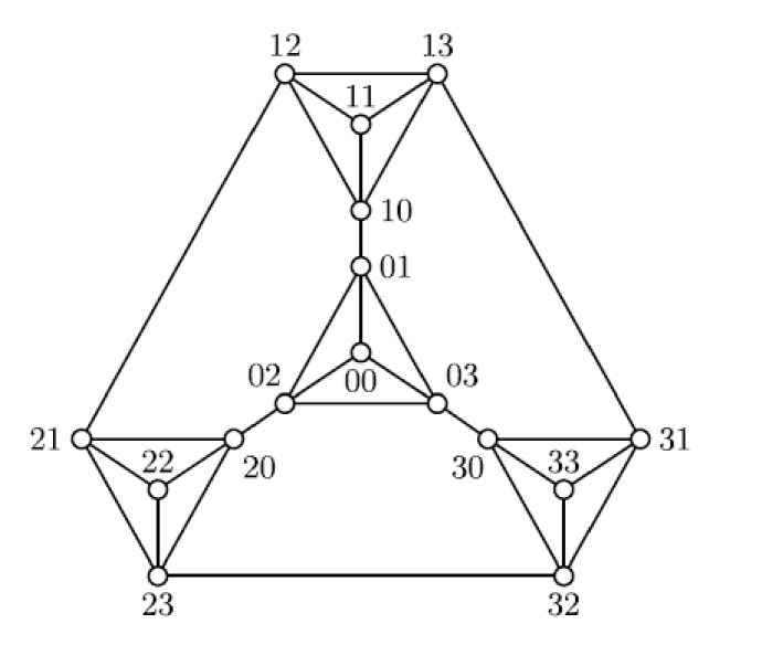
Figure 1: $S(2,4)$
Sierpiński graph $S(2,4)$ is shown in Figure 1. Note that $S(n,\ell)$ can be constructed recursively as follows: $S(1,\ell)$ is isomorphic to $K_{\ell}$ , which vertex set is 1-tuples set $\{0,\ldots,\ell-1\}$ . To construct $S(n,\ell)$ for $n>1$ , we take copies of $\ell$ times $S(n-1,\ell)$ and add the letter $i$ on the top of the vertices in $i$ -th copy of $S(n-1,\ell)$ , denoted by $S^{i}(n,\ell)$ . Note that there is exactly one edge (bridge edge) between $S^{i}(n,\ell)$ and $S^{j}(n,\ell)$ , $i\neq j$ , namely the edge between vertices $\langle ij\cdots j\rangle$ and $\langle ji\cdots i\rangle$ .
The vertices $(\underbrace{i,i,\cdots,i}_{n})$ , $i\in\{0,1,\ldots,\ell-1\}$ are the extreme vertices of $S(n,\ell)$ . Note that an extreme vertex $u$ of $S(n,\ell)$ has degree $d(u)=\ell-1$ . For $i\in\{0,\ldots,\ell-1\}$ and $n\geq 2$ , let $S^{i}(n-1,\ell)$ denote the subgraph of $S(n,\ell)$ induced by the vertices of the form $\{\langle iu_{1}\cdots u_{n-1}\rangle\,|\,0\leq u_{i}\leq\ell-1\}$ . The vertex set $V(S(n,\ell))$ can be partitioned into $\ell$ parts $V(S^{0}(n-1,\ell)),V(S^{1}(n-1,\ell)),\ldots,V(S^{\ell-1}(n-1,\ell))$ . For each $0\leq i\leq\ell-1$ , $S^{i}(n-1,\ell)$ is isomorphic to $S(n-1,\ell)$ . Note that $V(S(n,\ell))=V(S^{0}(n-1,\ell))\cup\cdots\cup V(S^{\ell-1}(n-1,\ell))$ and $S(n,\ell)$ is the graph obtained from $S^{0}(n-1,\ell),\ldots,S^{\ell-1}(n-1,\ell)$ by adding exactly one edge (bridge edge) between $S^{i}(n-1,\ell)$ and $S^{j}(n-1,\ell)$ , $i\neq j$ , and the bridge edge joins $\langle ij\cdots j\rangle$ and $\langle ji\cdots i\rangle$ (notices that $\langle ij\cdots j\rangle$ and $\langle ji\cdots i\rangle$ are extreme vertices of $S^{i}(n-1,\ell)$ and $S^{j}(n-1,\ell)$ , respectively, if we regard $S^{i}(n-1,\ell)$ and $S^{j}(n-1,\ell)$ as two copies of $S(n-1,\ell)$ ).
Sierpiński graphs generalize Hanoi graphs which can be viewed as “discrete” finite versions of a Sierpiński gasket [23, 10]. Xue considered the Hamiltionicity and path $t$ -coloring of Sierpiński-like graphs in [25]; furthermore, they proved that $Val(S(n,k))=Val(S[n,k])=\lfloor k/2\rfloor$ , where $Val(S(n,k))$ is the linear arboricity of Sierpiński graphs. We remark that although Sierpiński graphs are not regular, they are “almost” regular as the extreme vertices have degrees one less than the degrees of non-extreme vertices.
### 1.3 Preliminaries and our results
Chartrand et al. [4] and Li et al. [16] obtained the exact value of $\kappa_{k}(K_{n})$ .
**Theorem 1.1 ([16,4])**
*For every two integers $n$ and $k$ with $2\leq k\leq n$ ,
$$
\kappa_{k}(K_{n})=\lambda_{k}(K_{n})=n-\lceil k/2\rceil.
$$*
The following result is on the Hamiltonian decomposition of Sierpiński graphs.
**Theorem 1.2**
*[25] $(1)$ For even $\ell\geq 2$ , $S(n,\ell)$ can be decomposed into edge disjoint union of $\frac{\ell}{2}$ Hamiltonian paths of which the end vertices are extreme vertices. $(2)$ For odd $\ell\geq 3$ , there exist $\frac{\ell-1}{2}$ edge-disjoint Hamiltonian paths whose two end vertices are extreme vertices in $S(n,\ell)$ .*
In fact, Theorem 1.2 is used in the proof of Theorem 1.5, which give an lower bound for the generalized $k$ -edge connectivity of Sierpiński graphs $S(n,\ell)$ . We require the following result.
**Theorem 1.3 ([5,26])**
*Suppose that $G$ is a complete graph with $V(G)=\{v_{0},\cdots,v_{N-1}\}$ . If $N=2n$ , then $G$ can be decomposed into $n$ Hamiltonian paths
$$
\{i\in\{1,2,\ldots,n\}:\ L_{i}=v_{0+i}v_{1+i}v_{2n-1+i}v_{2+i}v_{2n-2+i}\cdots
v
_{n+1+i}v_{n+1}\},
$$
where the subscripts take modulo $2n$ . If $N=2n+1$ , then $G$ can be decomposed into $n$ Hamiltonian paths
$$
\{i\in\{1,2,\ldots,n\}:\ L_{i}=\ v_{0+i}v_{1+i}v_{2n+i}v_{2+i}v_{2n-1+i}\cdots
v
_{n+i}v_{n+1+i}\}
$$
and a matching $M=\{v_{n-i}v_{n+1}:\ i\in\{1,2,\ldots,n\}\}$ , where the subscripts take modulo $2n+1$ .*
The following result is derived from Theorem 1.3, and we will use it later.
**Corollary 1.4**
*Let $s$ be an integer with $s\leq\frac{N}{2}$ . Suppose that $G$ is the complete graph with $V(G)=\{v_{1},\cdots,v_{N}\}$ and $\mathcal{S}=\{\ \{v_{i_{1}},v_{i_{2}}\}:i\in\{1,2,\ldots,s\}\}$ is a collection of pairwise disjoint $2$ -subsets of $V(G)$ . Then there are $s$ edge-disjoint Hamiltonian paths $L_{1},\cdots,L_{s}$ such that $v_{i_{1}},v_{i_{2}}$ are endpoints of $L_{i}$ .*
Our main result is as follows.
**Theorem 1.5**
*$(i)$ For $3\leq k\leq\ell$ , we have
$$
\kappa_{k}(S(n,\ell))=\lambda_{k}(S(n,\ell))=\ell-\left\lceil k/2\right\rceil.
$$ $(ii)$ For $\ell+1\leq k\leq{\ell}^{n}$ , we have
$$
\kappa_{k}(S(n,\ell))\leq\left\lfloor\ell/2\right\rfloor\mbox{ and }\lambda_{k
}(S(n,\ell))=\left\lfloor\ell/2\right\rfloor.
$$*
## 2 Proof of Theorem 1.5
This section is organized as follows. We first introduce some notations, operations and auxiliary graphs that are used in the proof. Then we give a transitional theorem (Theorem 2.1), which is the main tool for the proof of Theorem 1.5. Theorem 2.1 will be proved by constructing an algorithm, and the proof takes up almost entire Section 2 (the proof is divided into two parts: the construction of algorithm and the proof of its correctness). Finally, we complete the proof of Theorem 1.5 by using Theorem 2.1.
### 2.1 Notations, operations and auxiliary graphs
For $1\leq s<n$ , by the definition of the Sierpiński graph $S(n,\ell)$ , we have that $G=S(n,\ell)$ consists of $\ell^{n-s}$ Sierpiński graphs $S(s,\ell)$ , and we call each such $S(s,\ell)$ an $s$ -atom of $G$ . Note that $\mathcal{P}=\{V(H):\ H\mbox{ is an }s\mbox{-atom of }G\}$ is a partition of $V(G)$ . We use $G_{s}$ to denote the graph $G/\mathcal{P}$ . It is obvious that $G_{s}$ is a simple graph and $G_{s}=S(n-s,\ell)$ . Note that $G_{n}$ is a single vertex and $G_{0}=G$ . For a vertex $u$ of $G_{s}$ , we use $A_{s,u}$ to denote the $s$ -atom of $G$ which is contracted into $u$ . See Figures 4, 4 and 4 for illustrations.
| Notation | Corresponding interpretation |
| --- | --- |
| $s$ -atom | A copy of $S(s,\ell)$ in $G=S(n,\ell)$ , where $0\leq s\leq n$ . |
| $G_{s}$ | The graph obtained from $G$ by contracting all $\ell^{n-s}$ $s$ -atoms in $G$ . |
| $A_{u,s}$ | The $s$ -atom in $G$ which is contracted into $u$ , where $u\in V(G_{s})$ . |
| $H^{u}$ | $G_{s-1}$ can be obtained form $G_{s}$ by expending each $u\in V(G_{s})$ to a complete graph $H^{u}=K_{\ell}$ . |
| $u^{e},v^{e}$ | If $e=uv$ is an edge of $G_{s}$ , then $e$ is also an edge of $G_{s-1}$ . let $u_{e},v_{e}$ denote endpoints of $e$ in $G_{s-1}$ such that $u_{e}\in H^{u}$ and $v_{e}\in H^{v}$ . |
| $U$ | The set of labelled vertices in $G$ ( $|U|=k$ ). |
| $U^{s}$ | The set of labelled vertices in $G_{s}$ . |
| $W^{u}$ | The set of labelled vertices in $H^{u}$ . |
Table 1: Notations for and their meanings.
Note that $G_{s-1}$ is the graph obtained from $G_{s}$ by replacing each vertex $u$ with a complete graph $K_{\ell}$ . We denote by $H^{u}$ the complete graph replacing $u$ (see Figures 4 and 4 for illustrations). For an edge $e=uv$ of $G_{s}$ , $e$ is also an edge of $G_{s-1}$ . We use $u_{e}$ and $v_{e}$ to denote the ends of $e$ in $G_{s-1}$ , respectively, such that $u_{e}\in V(H^{u})$ and $v_{e}\in V(H^{v})$ . (See Figure 5 for an illustration.)
Fix a subset $U$ of $V(G)$ arbitrary such that $|U|=k$ , where $3\leq k\leq\ell$ . For the graph $G_{s}$ , a vertex $u$ of $G_{s}$ is labelled if $V(A_{s,u})\cap U\neq\emptyset$ , and $u$ is unlabelled otherwise. We use $U^{s}$ to denote the set of labelled vertices of $G_{s}$ . For a labelled vertex $u$ of $G_{s}$ , let $W^{u}=V(H^{u})\cap U^{s-1}$ , that is, the set of labelled vertices in $H^{u}$ . See Figure 4 as an example, if $U=\{u_{000},u_{001},u_{013},u_{122}\}$ , then $U^{1}=\{u_{00},u_{01},u_{12}\}$ and $W^{u_{0}}=\{u_{00},u_{01}\}$ in Figure 4. For ease of reading, above notations and their meanings are summarized in Table 1.
We construct an out-branching $\overrightarrow{T}$ with vertex set $V(\overrightarrow{T})=\bigcup_{i\in\{0,1,\ldots,n\}}\{x:\ x\in V(G_{i})\}$ and arc set $A(\overrightarrow{T})=\{(x,y):\ y\in V(H^{x})\}$ . The root of $\overrightarrow{T}$ is denoted by $v_{root}$ (it is clear that $V(G_{n})=\{v_{root}\}$ ). For two different vertices $x,y$ of $V(\overrightarrow{T})$ , if there is a direct path from $x$ to $y$ , then we say that $x\prec y$ , and denote the directed path by $x\overrightarrow{T}y$ . The following result is straightforward.
**Fact 1**
*If $x_{i}\in V(\overrightarrow{T})$ for $i\in[p]$ and $x_{1}\prec x_{2}\prec\ldots\prec x_{p}$ , then $\sum_{i\in[p]}|W^{x_{i}}|\leq k+p-1$ .*
$u_{000}$ $u_{001}$ $u_{002}$ $u_{003}$ $u_{010}$ $u_{012}$ $u_{011}$ $u_{013}$ $u_{020}$ $u_{021}$ $u_{030}$ $u_{031}$ $u_{022}$ $u_{023}$ $u_{032}$ $u_{033}$ $u_{100}$ $u_{101}$ $u_{110}$ $u_{111}$ $u_{102}$ $u_{103}$ $u_{112}$ $u_{113}$ $u_{120}$ $u_{121}$ $u_{130}$ $u_{131}$ $u_{122}$ $u_{123}$ $u_{132}$ $u_{133}$ $u_{200}$ $u_{201}$ $u_{210}$ $u_{211}$ $u_{300}$ $u_{301}$ $u_{310}$ $u_{311}$ $u_{202}$ $u_{203}$ $u_{212}$ $u_{213}$ $u_{302}$ $u_{303}$ $u_{312}$ $u_{313}$ $u_{220}$ $u_{221}$ $u_{230}$ $u_{231}$ $u_{320}$ $u_{321}$ $u_{330}$ $u_{331}$ $u_{222}$ $u_{223}$ $u_{232}$ $u_{233}$ $u_{322}$ $u_{323}$ $u_{332}$ $u_{333}$ $A(2,u_{0})$ $A(2,u_{1})$
Figure 2: $G=G_{0}=S(3,4)$
$u_{00}$ $u_{01}$ $u_{02}$ $u_{03}$ $u_{10}$ $u_{11}$ $u_{12}$ $u_{13}$ $u_{20}$ $u_{21}$ $u_{30}$ $u_{31}$ $u_{22}$ $u_{23}$ $u_{32}$ $u_{33}$ $H^{u_{0}}$ $H^{u_{1}}$
Figure 3: The graph $G_{1}$
$u_{0}$ $u_{1}$ $u_{2}$ $u_{3}$
Figure 4: The graph $G_{2}$
### 2.2 A transitional theorem and its proof
In order to prove our main result (Theorem 1.5), we first prove the following transitional theorem by constructing $\ell-\left\lceil k/2\right\rceil$ internally disjoint $U$ -Steiner trees in $G$ .
**Theorem 2.1**
*Let $G=S(n,\ell)$ and $U\subseteq V(G)$ with $|U|=k$ ( $U$ is defined before), and let $c=\ell-\left\lceil k/2\right\rceil$ . For $0\leq s\leq n$ , $G_{s}$ has $c$ internally disjoint $U^{s}$ -Steiner trees $T_{1},\cdots,T_{c}$ such that the following statement holds.
1. For each $u\in U^{s}$ (say $u\in W^{v}$ and hence $v$ is a labelled vertex of $G_{s+1}$ if $s\neq n$ ) and $i\in[c]$ , $d_{T_{i}}(u)\leq 2$ .*
The rest part of this subsection is the proof of Theorem 2.1.
Proof of Theorem 2.1 Suppose that $s^{\prime}$ is the minimum integer such that $G_{s^{\prime}}$ has exactly one labelled vertex (note that $s^{\prime}$ exists since $G_{n}$ consists of a single labelled vertex). This means that $G_{s^{\prime}-1}$ has at least two labelled vertices. Let $v$ be the labelled vertex in $G_{s^{\prime}}$ . Then $U\subseteq A_{s^{\prime},v}$ . Thus, in order to find $c$ internally disjoint $U$ -Steiner trees of $G$ satisfying ( $\star$ ), we only need to find $c$ internally disjoint $U$ -Steiner trees in $A_{s^{\prime},v}$ satisfying ( $\star$ ). Hence, without loss of generality, we can assume that $G$ is a graph with
$$
|W^{v_{root}}|=|U^{n-1}|\geq 2. \tag{1}
$$
Therefore, $|U^{i}|\geq 2$ for each $i\leq n-1$ . $u_{11}$ $u_{12}$ $u_{13}$ $u_{24}$ $u_{21}$ $u_{22}$ $u_{23}$ $u_{24}$ $u_{31}$ $u_{32}$ $u_{41}$ $u_{42}$ $u_{33}$ $u_{34}$ $u_{43}$ $u_{44}$ $e$ $u_{e}$ $v_{e}$ $u$ $v$ $e$ $G_{1}$ $G_{2}$
Figure 5: From graph $G_{1}$ to $G_{2}$ by $u_{e}v_{e}$ contraction edge $uv$ .
The proof is technical and is via induction. Note that since $G_{n}$ is a single vertex and $G=G_{0}$ , the induction is from $G_{n}$ to $G_{0}$ . The basic idea is to use the $U^{s}$ -Steiner trees of $G_{s}$ to construct appropriate $U^{s-1}$ -Steiner trees of $G_{s-1}$ . Since each vertex in $G_{s}$ corresponds to a complete graph in $G_{s-1}$ , it is not a straightforward process to extend $U^{s}$ -Steiner trees of $G_{s}$ to $U^{s-1}$ -Steiner trees of $G_{s-1}$ .
If $s=n$ , then each $T_{i}$ in $G_{n}$ is the empty graph and the result holds. Thus, suppose $s\leq n-1$ . Hence, the labelled vertex $v$ of $G_{s+1}$ always exists. The following implies that the result holds for $s=n-1$ . Note that $U^{n-1}=W^{v_{root}}$ .
**Claim 1**
*If $s=n-1$ , then we can construct $c$ internally disjoint $U^{s}$ -Steiner trees, say $T_{1},\ldots,T_{c}$ , such that for each $i\in[c]$ and $u\in U^{s}$ , $d_{T_{i}}(u)\leq 2$ . Moreover,
1. $(i)$ If $|U^{s}|\leq\lceil k/2\rceil$ , then for each $i\in[c]$ and $u\in U^{s}$ , $d_{T_{i}}(u)=1$ ;
1. $(ii)$ otherwise, for each $u\in U^{s}$ , there are at most $|U^{s}|-\lceil k/2\rceil$ internally disjoint $U^{s}$ -Steiner trees $T_{i}$ such that $d_{T_{i}}(u)=2$ .*
* Proof*
Note that $G_{n-1}=S(1,\ell)=K_{\ell}$ . Suppose $|U^{n-1}|\leq\left\lceil k/2\right\rceil$ . Then $|V(G_{n-1})-U^{n-1}|\geq\ell-\left\lceil k/2\right\rceil=c$ and we can choose $c$ stars of $\{x\vee U^{n-1}:\ x\in V(G_{n-1})-U^{n-1}\}$ as internally disjoint $U^{n-1}$ -Steiner trees $T_{1},\ldots,T_{c}$ . It is easy to verify that $d_{T_{i}}(u)=1$ for $i\in[c]$ and $u\in U^{n-1}$ . Suppose $|U^{n-1}|\geq\lceil k/2\rceil$ . Since $|U^{n-1}|\leq k$ , it follows that $0\leq|U^{n-1}|-\left\lceil k/2\right\rceil\leq\lfloor|U^{n-1}|/2\rfloor$ . By Corollary 1.4, there are $|U^{n-1}|-\left\lceil k/2\right\rceil$ edge-disjoint Hamiltonian paths in $G_{n-1}[U^{n-1}]$ . So, we can choose $c$ internally disjoint $U^{n-1}$ -Steiner trees consisting of $|U^{n-1}|-\left\lceil k/2\right\rceil$ edge-disjoint Hamiltonian paths in $G_{n-1}[U^{n-1}]$ and $\ell-|U^{n-1}|$ stars $\{x\vee U^{n-1}:\ x\in V(G_{n-1})-U^{n-1}\}$ . It is easy to verify that $d_{T_{i}}(u)\leq 2$ for $i\in[c]$ and $u\in U^{n-1}$ , and there are at most $|U^{n-1}|-\left\lceil k/2\right\rceil$ internally disjoint $U^{n-1}$ -Steiner trees $T_{i}$ such that $d_{T_{i}}(u)=2$ . ∎
Our proof is a recursive process that the $c$ internally disjoint $U^{s}$ -Steiner trees of $G_{s}$ are constructed by using the $c$ internally disjoint $U^{s+1}$ -Steiner trees of $G_{s+1}$ . We will find some ways to construct the $c$ internally disjoint $U^{s}$ -Steiner trees such that $(\star)$ holds. In the finial step, the $c$ internally disjoint $U$ -Steiner trees in $G_{0}=G$ will be obtained. We have proved that the result holds for $s\in\{n,n-1\}$ . Now, suppose that we have constructed $c$ internally disjoint $U^{s+1}$ -Steiner trees, say $\mathcal{F}=\{F_{1},\ldots,F_{c}\}$ , and the trees satisfy ( $\star$ ), where $s\in\{0,\ldots,n-1\}$ . We need to construct $c$ internally disjoint $U^{s}$ -Steiner trees $\mathcal{T}=\{T_{1},\ldots,T_{c}\}$ of $G_{s}$ satisfying ( $\star$ ).
Recall that each edge of $G_{s+1}$ is also an edge of $G_{s}$ . In addition, let $E_{u,i}$ denote the set of edges in $F_{i}$ incident with the labelled vertex $u$ in $G_{s}$ and let $V_{u,i}=\{u_{e}:\ e\in E_{u,i}\}$ (recall that the edge $e=uw$ in $G_{s+1}$ is denoted by $e=u_{e}w_{e}$ in $G_{s}$ , where $u_{e}\in V(H^{u})$ and $w_{e}\in V(H^{w})$ ). Note that $E_{u,i}$ and $V_{u,i}$ are the subsets of $E(G_{s})$ and $V(G_{s})$ , respectively.
Our aim is to construct internally disjoint $U^{s}$ -Steiner trees $T_{1},\ldots,T_{c}$ that is obtained from $U^{s+1}$ -Steiner trees $F_{1},\ldots,F_{c}$ . So, we need to “blow” up each vertex $w$ of $G_{s+1}$ into $H^{w}$ and find internally disjoint $W^{w}$ -Steiner trees $F_{1}^{w},\ldots,F_{c}^{w}$ of $H^{w}$ ( $F_{i}^{w}$ may be the empty graph if $w$ is a unlabelled vertex) such that
$$
\mathcal{T}=\left\{T_{i}=F_{i}\cup\bigcup_{w\in V(G_{s+1})}F_{i}^{w}:\ i\in[c]
\right\}.
$$
Each $F_{i}^{w}$ can be constructed as follows.
- If $w$ is a labelled vertex of $G_{s+1}$ , then $w$ is in each $U^{s+1}$ -Steiner tree of $\mathcal{F}$ . We choose $c$ internally disjoint $W^{w}$ -Steiner trees $F_{1}^{w},\ldots,F_{c}^{w}$ of $H^{w}$ such that $V_{w,i}\subseteq V(F_{i}^{w})$ for each $i\in[c]$ .
- If $w$ is an unlabelled vertex, then $w$ is in at most one $U^{s+1}$ -Steiner tree of $\mathcal{F}$ . For each $i\in[c]$ , if $w\in V(F_{i})$ , then let $F_{i}^{w}$ be a spanning tree of $H^{w}$ ; if $w\notin V(F_{i})$ , then let $F_{i}^{w}$ be the empty graph.
For $i\in[c]$ , let $E_{i}=E(F_{i})\cup\bigcup_{w\in V(G_{s+1})}E(F_{i}^{w})$ and let $T_{i}=G_{s}[E_{i}]$ . It is obvious that $T_{1},\ldots,T_{c}$ are internally disjoint $U^{s}$ -Steiner trees. We need to ensure that each labelled vertex of $G^{s}$ satisfies ( $\star$ ).
In fact, without loss of generality, we only need to choose an arbitrary labelled vertex $u\in G_{s+1}$ and prove that each vertex of $W^{u}$ satisfies ( $\star$ ). This is because $F_{i}^{w}$ is clear when $w$ is an unlabelled vertex (in the case $F_{i}^{w}$ is either a spanning tree of $H^{w}$ or the empty graph). By Eq. (1) and Fact 1, $|W^{u}|\leq k-1$ since $u\neq v_{root}$ .
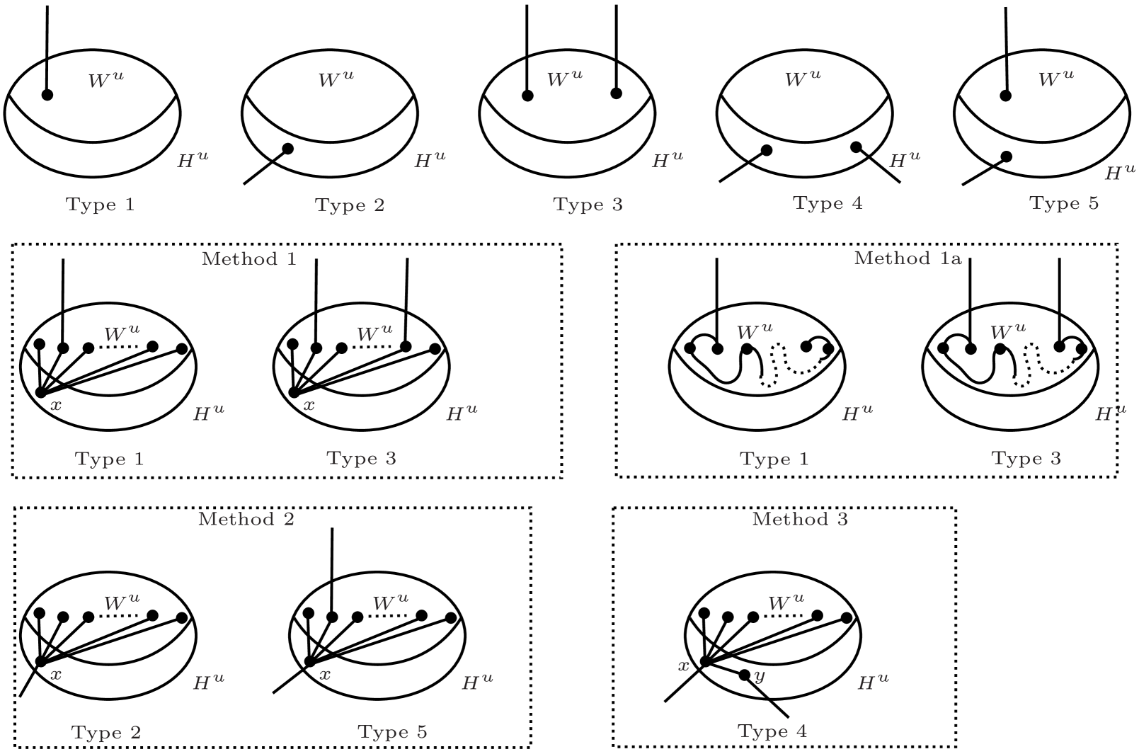
Since $d_{F_{i}}(u)\leq 2$ for each $i\in[c]$ and $u\in U^{s}$ , it follows that $|E_{u,i}|=|V_{u,i}|\leq 2$ . Therefore, we can divide $F_{1},\ldots,F_{c}$ into the following five types on $u$ :
Type 1: $|V_{u,i}|=1$ and $V_{u,i}\subseteq W^{u}$ .
Type 2: $|V_{u,i}|=1$ and $V_{u,i}\nsubseteq W^{u}$ .
Type 3: $|V_{u,i}|=2$ and $V_{u,i}\subseteq W^{u}$ .
Type 4: $|V_{u,i}|=2$ and $V_{u,i}\cap W^{u}=\emptyset$ .
Type 5: $|V_{u,i}|=2$ and $|V_{u,i}\cap W^{u}|=1$ .
If $F_{i}$ is a graph of Type $j\ (1\leq j\leq 5)$ on $u$ , then we also call $F_{i}^{u}$ a $W^{u}$ -Steiner tree of Type $j$ . Suppose there are $n_{j}(u)$ trees $F_{i}$ that belong to Type $j$ on $u$ for $j\in[5]$ . Then
$$
\displaystyle\sum_{i=1}^{5}n_{j}(u)=c. \tag{2}
$$
It is obvious that $n_{j}(v_{root})=0$ for each $j\in[5]$ . Let
$$
R(u)=V(H^{u})-W^{u}-\bigcup_{i\in[c]}V_{u,i}.
$$
Note that $R(u)$ is the set of unlabelled vertices in $G_{s}$ , which will be used to construct the $W^{u}$ -Steiner trees in $H^{u}$ . It is clear that
$$
|R(u)|=\ell-|W^{u}|-[n_{2}(u)+2n_{4}(u)+n_{5}(u)]. \tag{3}
$$
<details>
<summary>x2.png Details</summary>
### Visual Description
## Diagram: Geometric/Topological Classification of Types and Methods
### Overview
The image presents a series of schematic diagrams illustrating topological or geometric configurations, likely related to handlebody theory, surface topology, or graph embeddings. The diagrams are organized into two sections: a top row defining five distinct "Types" (1 through 5) and a lower section grouping these types into "Methods" (1, 1a, 2, and 3). Each diagram features an ellipse representing a space, with internal points and connecting lines indicating structural relationships.
### Components/Axes
* **Labels:**
* **$W^u$**: Denotes the upper region or interior of the ellipse.
* **$H^u$**: Denotes the lower region or boundary of the ellipse.
* **$x$**: A specific basepoint or root vertex located on the left side of the ellipse boundary.
* **$y$**: A specific point located on the lower boundary of the ellipse (only in Method 3).
* **Types 1-5**: Classifications of the geometric configuration.
* **Methods 1, 1a, 2, 3**: Groupings of specific types, indicating operations or constructions.
### Detailed Analysis
#### Top Row: Baseline Types
* **Type 1**: An ellipse with one point on the upper boundary ($W^u$) and one vertical line extending upward from it.
* **Type 2**: An ellipse with one point on the lower boundary ($H^u$) and one line extending downward from it.
* **Type 3**: An ellipse with two points on the upper boundary ($W^u$), each with a vertical line extending upward.
* **Type 4**: An ellipse with two points on the lower boundary ($H^u$), each with a line extending downward.
* **Type 5**: An ellipse with one point on the upper boundary ($W^u$) and one point on the lower boundary ($H^u$), with lines extending both upward and downward.
#### Boxed Methods
* **Method 1 (Left Box)**:
* **Type 1**: A central point $x$ on the left is connected by solid lines to four points on the upper boundary ($W^u$).
* **Type 3**: Similar to Type 1, but with an additional vertical line extending upward from the rightmost point on the upper boundary.
* **Method 1a (Right Box)**:
* **Type 1**: Points on the upper boundary ($W^u$) are connected to each other via curved, dashed lines.
* **Type 3**: Similar to Type 1, but with an additional vertical line extending upward from the rightmost point on the upper boundary.
* **Method 2 (Bottom Left Box)**:
* **Type 2**: A central point $x$ on the left is connected by solid lines to four points on the upper boundary ($W^u$).
* **Type 5**: Similar to Type 2, but with an additional vertical line extending upward from the rightmost point on the upper boundary.
* **Method 3 (Bottom Right Box)**:
* **Type 4**: A central point $x$ on the left is connected by solid lines to four points on the upper boundary ($W^u$). Additionally, there is a point $y$ on the lower boundary ($H^u$) connected to the central point $x$.
### Key Observations
* **Structural Progression**: The "Methods" appear to be applying a "star graph" structure (rooted at $x$) to the baseline "Types" defined in the top row.
* **Line Styles**:
* **Solid lines** (Methods 1, 2, 3) suggest direct connections or edges in a graph.
* **Dashed/Curved lines** (Method 1a) suggest a different type of relationship, possibly representing paths, homotopy, or specific boundary interactions distinct from the solid-line connections.
* **Point $x$**: In all boxed methods, $x$ acts as a primary hub or root vertex from which connections emanate to the rest of the structure.
### Interpretation
This diagram likely originates from a mathematical paper concerning **Heegaard splittings**, **train tracks on surfaces**, or **handlebody decompositions**.
* **The "Types"**: These represent fundamental building blocks or "handles" of a manifold. The distinction between $W^u$ (upper) and $H^u$ (lower) suggests a splitting of a surface or 3-manifold.
* **The "Methods"**: These represent different ways to construct or modify these manifolds.
* **Method 1/2/3** likely represent the construction of a graph embedded within the manifold, where $x$ is a basepoint.
* **Method 1a** is distinct because it uses dashed lines, implying it describes a different topological operation—perhaps a "cut-and-paste" operation or a specific type of curve system on the surface that differs from the graph-based connections in the other methods.
* **Peircean Investigative Note**: The consistency of the "Type" labels across the top row and the boxed sections suggests that the boxed sections are *instantiations* or *applications* of these types within a larger, more complex system. The transition from Type 1 to Type 3 in the boxed sections (adding an extra vertical line) suggests an incremental increase in complexity or "genus" of the underlying structure.
</details>
Figure 6: Five types and methods 1, 1a, 2 and 3.
We have the following five methods to choose $F_{1}^{u},\ldots,F_{c}^{u}$ for the labelled vertex $u\in G_{s+1}$ (see Figure 6).
Method 1 If $F_{i}$ is a graph of Type 1 and $|W^{u}|\geq 2$ , or $F_{i}$ is a graph of Type 3, then let $F^{u}_{i}=x\vee W^{u}$ , where $x\in R(u)$ .
Method 1a If $F_{i}$ is a graph of Type 1 and $|W^{u}|\geq 2$ , then let $F^{u}_{i}$ be a Hamiltonian path of $H^{u}[W^{u}]$ such that the vertex in $V_{u,i}$ is an endpoint of this Hamiltonian path; if $F_{i}$ is a graph of Type 3, then let $F^{u}_{i}$ be a Hamiltonian path of $H^{u}[W^{u}]$ such that the endpoints of $F_{i}$ are two vertices in $V_{u,i}$ .
Method 2 If $F_{i}$ is a graph of Type 2 or Type 5, say $x$ is the only vertex of $V_{u,i}$ with $x\notin W^{u}$ , then let $F^{u}_{i}=x\vee W^{u}$ .
Method 3 If $F_{i}$ is a graph of Type 4, say $V_{u,i}=\{x,y\}$ , then let $F^{u}_{i}=xy\cup(x\vee W^{u})$ .
Method 4 If $F_{i}$ is a graph of Type 1 and $|W^{u}|=1$ , then let $F_{i}^{u}$ be the empty graph.
It is worth noting that the method is deterministic if $F_{i}^{u}$ is a graph of Types 2, 4 and 5, or $F_{i}^{u}$ is a graph of Type 1 and $|W^{u}|=1$ . So we firstly construct these $F_{i}^{u}$ s by using Methods 2, 3 and 4, respectively, and then construct $F^{u}_{i}$ s of Type 1 with $|W^{u}|\geq 2$ and construct $F^{u}_{i}$ s of Type 3 by using Method 1 or Method 1a.
The following is an algorithm constructing $c$ internally disjoint $U$ -Steiner trees of $G$ .
Input: $U$ , $c$ and $G=S(n,\ell)$ with $|W^{root}|\geq 2$
Output: $c$ internally disjoint $U$ -Steiner trees $T^{\prime}_{1},T^{\prime}_{2},\ldots,T^{\prime}_{c}$ of $G$
1 $T^{\prime}_{1},T^{\prime}_{2},\ldots,T^{\prime}_{c}$ are empty graphs;
2 $s=n$ //(* in initial step, $G^{n}$ is a single vertex*);
3 for $s\geq 1$ do
4 for each vertex $u$ of $G_{s}$ do
5 if $u$ is an unlabelled vertex then
6 for $1\leq i\leq c$ do
7 if $u$ is a vertex of $F_{i}$ then
8 $F_{i}^{u}$ is a spanning tree of $H^{u}$ ;
9 else
10 $\ F_{i}^{u}$ is is the empty graph;
11 end if
12 $T^{\prime}_{i}=T^{\prime}_{i}\cup F_{i}^{u}$ ;
13 $i=i+1$ ;
14
15 end for
16
17 end if
18
19 if $u$ is a labelled vertex then
20 $\mu=|R(u)|$ ;
21 for $1\leq i\leq c$ do
22
23 if $T^{\prime}_{i}$ is of Type 2 or Type 5 then
24 construct $F_{i}^{u}$ by using Method 2;
25
26 end if
27
28 if $T^{\prime}_{i}$ is of Type 4 then
29 construct $F_{i}^{u}$ by using Method 3;
30
31 end if
32
33 if $T^{\prime}_{i}$ is of Type 1 and $|W^{u}|=1$ then
34 construct $F_{i}^{u}$ by using Method 4;
35
36 end if
37
38 if either $T^{\prime}_{i}$ is of Type 1 and $|W^{u}|\geq 2$ , or $T^{\prime}_{i}$ is of Type 3 then
39 if $\mu>0$ then
40 construct $F_{i}^{u}$ by using Method 1;
41 $\mu=\mu-1$ ;
42
43 end if
44
45 if $\mu\leq 0$ then
46 construct $F_{i}^{u}$ by using Method 1a;
47
48 end if
49
50 end if
51
52 $T^{\prime}_{i}=T^{\prime}_{i}\cup F_{i}^{u}$ ;
53 $i=i+1$ ;
54
55 end for
56
57 end if
58
59 end for
60 $s=s-1$ ;
61
62 end for
Algorithm 1 The construction of $c$ internally disjoint $U$ -Steiner trees of $G$
Algorithm 1 is an algorithm for finding $c$ internally disjoint $U$ -Steiner trees of $G$ . For each step of $s$ , the algorithm will construct $c$ internally disjoint $U^{s-1}$ -steiner trees $T^{\prime}_{1},T^{\prime}_{2},\ldots,T^{\prime}_{c}$ . For convenience, we denote each $T_{i}^{\prime}$ by $T_{i}^{s}$ after the $s$ step of outer “for”, that is, $T_{1}^{s},T_{2}^{s},\ldots,T_{c}^{s}$ are $c$ internally disjoint $U^{s}$ -Steiner trees in $G^{s}$ generated in Algorithm 1. If Algorithm 1 is correct, then Lines 16–40 indicate that $d_{T^{\prime}_{i}}(x)\leq 2$ for any $x\in W^{u}$ , and hence ( $\star$ ) always holds.
We now check the correctness of the algorithm. Since $F_{i}^{u}$ is deterministic when $u$ is an unlabelled vertex (Lines 5–15 of Algorithm 1), and $F_{i}^{u}$ is deterministic if $u$ is a labelled vertex and either $F_{i}^{u}$ is a graph of Types 2, 4 and 5, or $F_{i}^{u}$ is a graph of Type 1 and $|W^{u}|=1$ (Lines 19–27 of Algorithm 1), we only need to talk about the labelled vertex $u$ with $|W^{u}|\geq 2$ and check the correctness of Lines 28–36 of Algorithm 1. That is, to ensure that there exist $n_{1}(u)$ $F_{i}^{u}$ s of Type 1 and $n_{3}(u)$ $F_{i}^{u}$ s of Type 3. If $F_{i}^{u}$ is constructed by Method 1, then $F_{i}^{u}$ is a star with center in $R(u)$ (say the center of the star is $a_{i}$ ); if $F_{i}^{u}$ is constructed by Method 1a, then $F_{i}^{u}$ is a Hamiltonian path of $H^{u}$ with endpoints in $V_{u,i}$ . Since $a_{i}$ s are pairwise differently and are contained in $R(u)$ , and $H^{u}$ has at most $\lfloor|W^{u}|/2\rfloor$ Hamiltonian paths to afford by Corollary 1.4, we only need to ensure that $|R(u)|+\lfloor|W^{u}|/2\rfloor\geq n_{1}(u)+n_{3}(u)$ . Thus, we only need to prove the following result.
**Lemma 2.1**
*For each labelled vertex $u\in V(G_{s})$ with $|W^{u}|\geq 2$ , Ineq.
$$
\displaystyle n_{1}(u)+n_{3}(u)-|R(u)|\leq\lfloor|W^{u}|/2\rfloor \tag{4}
$$
holds.*
* Proof*
By Eqs. (2) and (3),
| | $\displaystyle n_{1}(u)+n_{3}(u)-|R(u)|$ | $\displaystyle=n_{1}(u)+n_{3}(u)-[\ell-|W^{u}|-n_{2}(u)-2n_{4}(u)-n_{5}(u)]$ | |
| --- | --- | --- | --- |
Since $c=\ell-\lceil k/2\rceil$ , it follows that
$$
\displaystyle n_{1}(u)+n_{3}(u)-|R(u)|=n_{4}(u)+|W^{u}|-\lceil k/2\rceil. \tag{5}
$$ Before the proof of Lemma 2.1, we give a series of claims as preliminaries.
**Claim 2**
*Suppose that $a\in V(v_{root}\overrightarrow{T}u)$ is a labelled vertex with $a\in U^{\iota}$ , where $1\leq\iota\leq n$ . If $|W^{a}|=1$ (say $W^{a}=\{x\}$ ), then $n_{5}(a)\leq 1$ . Moreover,
1. if $n_{5}(a)=1$ , then $n_{4}(x)\leq 1$ ;
1. if $n_{5}(a)=0$ , then $n_{3}(x)=n_{4}(x)=n_{5}(x)=0$ .*
* Proof*
Note that $x\in U^{\iota-1}$ . in Algorithm 1 (Lines 18–39), if $T_{i}^{\iota}$ is not a tree of Type 5 on $a$ , then $F_{i}^{a}$ is chosen such that $d_{T_{i}^{\iota-1}}(x)=1$ (here $W^{a}=\{x\}$ ); if $T^{\iota}_{i}$ is a tree of Type 5 on $a$ , then $F_{i}^{a}$ is chosen such that $d_{T_{i}^{\iota-1}}(x)=2$ . Since $|W^{a}|=1$ , there is at most one $T^{\iota}_{i}$ of Type 5 on $a$ , and hence $n_{5}(a)\leq 1$ . Furthermore, if $n_{5}(a)=1$ , then there is exact one $T_{i}^{\iota-1}$ in $G^{\ell-1}$ such that $d_{T_{i}^{\iota-1}}(x)=2$ . Hence, $n_{4}(x)\leq 1$ . If $n_{5}(a)=0$ , then $d_{T_{i}^{\iota-1}}(x)=1$ for each $T_{i}^{\iota-1}$ . Therefore, $n_{3}(x)=n_{4}(x)=n_{5}(x)=0$ . ∎
**Claim 3**
*Suppose that $a,b$ are two labelled vertices of $v_{root}\overrightarrow{T}u$ and $a\in W^{b}$ , where $a\in U^{\iota}$ for some $\iota\in[n]$ . Then there are at most $\max\{1,n_{1}(b)+n_{3}(b)-|R(b)|+1\}$ $T_{i}^{\iota}$ s such that $d_{T_{i}^{\iota}}(a)=2$ . Furthermore, $n_{4}(a)\leq\max\{1,n_{1}(b)+n_{3}(b)-|R(b)|+1\}$ .*
* Proof*
Since $a\in W^{b}$ and $a\in U^{\iota}$ , it follows that $b\in U^{\iota+1}$ . For an $i\in[c]$ with $d_{T_{i}^{\iota}}(a)=2$ , we have that either $F_{i}^{b}$ is a Hamiltonian path of the clique $H^{b}[W^{b}]$ , or $a\in V_{b,i}\cap W^{b}$ for some $i\in[c]$ (recall that $V_{b,i}=\{z\in V(H^{b}):z\mbox{ is an end vertex of some edge in }E_{b,i}\}$ , where $E_{b,i}$ is the set of edges in $T_{i}^{\iota+1}$ incident with $b$ ). Hence, if there are $h$ edge-disjoint $F_{i}^{b}$ s that are constructed as Hamiltonian paths of $H^{b}[W^{b}]$ , then there are at most $h+1$ internally disjoint $U^{\iota}$ -Steiner trees $T_{i}^{\iota}$ such that $d_{T_{i}^{\iota}}(a)=2$ . By the definition of $n_{4}(a)$ , we have that $n_{4}(a)\leq h+1$ . In Algorithm 1 (Lines 28–36), if $n_{1}(b)+n_{3}(b)-|R(b)|>0$ , then there are at most $n_{1}(b)+n_{3}(b)-|R(b)|$ $F_{i}^{b}$ s that are constructed as Hamiltonian paths in $H^{b}[W^{b}]$ ; if $n_{1}(b)+n_{3}(b)-|R(b)|\leq 0$ , there is no $F_{i}^{b}$ that is constructed as a Hamiltonian path in $H^{b}[W^{b}]$ . Hence, $h\leq\max\{0,n_{1}(b)+n_{3}(b)-|R(b)|\}$ . Thus, there are at most $\max\{1,n_{1}(b)+n_{3}(b)-|R(b)|+1\}$ internally disjoint $U^{\iota}$ -Steiner trees $T_{i}^{\iota}$ such that $d_{T_{i}^{\iota}}(a)=2$ , and $n_{4}(a)\leq\max\{1,n_{1}(b)+n_{3}(b)-|R(b)|+1\}$ . ∎
**Claim 4**
*Let $a\in V(v_{root}\overrightarrow{T}u)$ be a labelled vertex, where $a\in U^{\iota}$ for some $\iota\in[n]$ . If $n_{4}(a)\leq 1$ and $2\leq|W^{a}|\leq\left\lceil k/2\right\rceil-1$ , then $n_{1}(a)+n_{3}(a)-|R(a)|\leq 0$ . Moreover, for each vertex $x\in W^{a}$ , there is at most one $T_{i}^{\iota-1}$ such that $d_{T_{i}^{\iota-1}}(x)=2$ .*
* Proof*
Since $n_{4}(a)\leq 1$ and $|W^{a}|\leq\left\lceil k/2\right\rceil-1$ , it follows from Eq. (5) that $n_{1}(a)+n_{3}(a)-|R(a)|=|W^{a}|-\left\lceil k/2\right\rceil+1\leq 0.$ By Claim 3, for each vertex $x\in W^{a}$ , there is at most one $T_{i}^{a}$ such that $d_{T_{i}^{\iota-1}}(x)\leq 2$ . ∎
**Claim 5**
*Let $a\in V(v_{root}\overrightarrow{T}u)$ be a labelled vertex, where $a\in U^{\iota}$ for some $\iota\in[n]$ . If $n_{4}(a)\leq 1$ and $\left\lceil k/2\right\rceil\leq|W^{a}|\leq k-1$ , then $n_{1}(a)+n_{3}(a)-|R(a)|\leq\lfloor|W^{a}|/2\rfloor$ . Moreover, for each $x\in W^{a}$ ,
1. if $n_{4}(a)=1$ , then there are at most $|W^{a}|-\left\lceil k/2\right\rceil+2$ internally disjoint $U^{\iota-1}$ -Steiner trees $T_{i}^{\iota-1}$ such that $d_{T_{i}^{\iota-1}}(x)=2$ ;
1. if $n_{4}(a)=0$ , then there are at most $|W^{a}|-\left\lceil k/2\right\rceil+1$ internally disjoint $U^{\iota-1}$ -Steiner trees $T_{i}^{\iota-1}$ such that $d_{T_{i}^{\iota-1}}(x)=2$ .*
* Proof*
Since $n_{4}(a)\leq 1$ , it follows from Eq. (5) that
| | $\displaystyle n_{1}(a)+n_{3}(a)-|R(a)|$ | $\displaystyle\leq|W^{a}|-\left\lceil k/2\right\rceil+n_{4}(a)$ | |
| --- | --- | --- | --- |
and the equality indicates $n_{4}(a)=1$ . If $|W^{a}|\leq k-2$ , then
$$
n_{1}(a)+n_{3}(a)-|R(a)|\leq|W^{a}|-\left\lceil(|W^{a}|+2)/2\right\rceil+1\leq
\left\lfloor|W^{a}|/2\right\rfloor;
$$
if $|W^{a}|=k-1$ and $k$ is even, then
$$
n_{1}(a)+n_{3}(a)-|R(a)|=|W^{a}|-\left\lceil(|W^{a}|+1)/2\right\rceil+1=\left
\lfloor(|W^{a}|+1)/2\right\rfloor=\left\lfloor|W^{a}|/2\right\rfloor;
$$
if $|W^{a}|=k-1$ and $k$ is odd, then
$$
n_{1}(a)+n_{3}(a)-|R(a)|=(k-1)-\left\lceil k/2\right\rceil+1\leq\left\lfloor k
/2\right\rfloor=\left\lfloor(k-1)/2\right\rfloor=\left\lfloor|W^{a}|/2\right\rfloor.
$$
Therefore, $n_{1}(a)+n_{3}(a)-|R(a)|\leq\left\lfloor|W^{a}|/2\right\rfloor$ . By Eq. (5) and Claim 3, if $n_{4}(a)=1$ , then for each vertex $x\in W^{a}$ , there are at most $n_{1}(a)+n_{3}(a)-|R(a)|+1=|W^{a}|-\left\lceil k/2\right\rceil+2$ internally disjoint $U^{\iota-1}$ -Steiner trees $T_{i}^{\iota-1}$ such that $d_{T_{i}^{\iota-1}}(x)=2$ ; if $n_{4}(a)=0$ , then for each vertex $x\in W^{a}$ , there are at most $n_{1}(a)+n_{3}(a)-|R(a)|+1=|W^{u}|-\left\lceil k/2\right\rceil+1$ internally disjoint $U^{\iota-1}$ -Steiner trees $T_{i}^{\iota-1}$ such that $d_{T_{i}^{\iota-1}}(x)=2$ . ∎
**Claim 6**
*Suppose $a,b\in V(\overrightarrow{T})$ , $a\prec b$ and $a\overrightarrow{T}b=az_{1}z_{2}\ldots z_{p}b$ , where $a\in U^{\iota}$ for some $\iota\in[n]$ . If $|W^{z_{i}}|\leq\lceil k/2\rceil-1$ for each $i\in[p]$ , and either $|W^{a}|=1$ or $2\leq|W^{a}|\leq\lceil k/2\rceil-1$ and $n_{4}(a)\leq 1$ , then $n_{4}(b)\leq 1$ .*
* Proof*
Since $a\in U^{\iota}$ , it follows that $z_{q}\in U^{\iota-q}$ for each $q\in[p]$ and $b\in U^{\iota-p-1}$ . Since $|W^{a}|=1$ or $2\leq|W^{a}|\leq\lceil k/2\rceil-1$ and $n_{4}(a)\leq 1$ , by Claims 2 and 4, there are at most one $T_{i}^{\iota-1}$ such that $d_{T_{i}^{\iota-1}}(z_{1})=2$ . Hence, $n_{4}(z_{1})\leq 1$ . Since $|W^{z_{1}}|\leq\lceil k/2\rceil-1$ and $n_{4}(z_{1})\leq 1$ , by Claims 2 and 4, there are at most one $T_{i}^{\iota-2}$ such that $d_{T_{i}^{\iota-2}}(z_{2})=2$ . Hence, $n_{4}(z_{2})\leq 1$ . Repeat this progress, we can get that $n_{4}(z_{p})\leq 1$ . Since $|W^{z_{p}}|\leq\lceil k/2\rceil-1$ and $n_{4}(z_{p})\leq 1$ , by Claims 2 and 4, there are at most one $T_{i}^{\iota-p-1}$ such that $d_{T_{i}^{\iota-p-1}}(b)=2$ . Hence, $n_{4}(b)\leq 1$ . ∎
**Claim 7**
*Suppose $|W^{v_{root}}|\leq\lceil k/2\rceil$ , $b\in V(\overrightarrow{T})$ and $v_{root}\overrightarrow{T}b=v_{root}z_{1}z_{2}\ldots z_{p}b$ . If $|W^{z_{i}}|=1$ for each $i\in[p]$ , then $n_{4}(b)=0$ .*
* Proof*
Since $|W^{v_{root}}|\leq\lceil k/2\rceil$ , by Claim 1, $d_{T_{i}^{n-1}}(z_{1})=1$ for each $U^{n-1}$ -Steiner tree $T_{i}^{n-1}$ . Hence, $n_{3}(z_{1})=n_{4}(z_{1})=n_{5}(z_{1})=0$ . Since $|W^{z_{1}}|=1$ and $n_{5}(z_{1})=0$ , by the second statement of Claim 2, $n_{3}(z_{2})=n_{4}(z_{2})=n_{5}(z_{2})=0$ . Since $|W^{z_{2}}|=1$ and $n_{5}(z_{2})=0$ , by the second statement of Claim 2, $n_{3}(z_{3})=n_{4}(z_{3})=n_{5}(z_{3})=0$ . Repeat this process, we get that $n_{4}(b)=0$ . ∎
**Claim 8**
*Suppose that $a,b$ are two labelled vertices and $a\in W^{b}$ , where $a\in U^{\iota}$ for some $\iota\in[n]$ . If $k$ is even and $|W^{b}|=|W^{a}|=k/2$ , then $n_{1}(a)+n_{3}(a)-|R(a)|\leq\lfloor|W^{a}|/2\rfloor$ and the following hold.
1. If $b=v_{root}$ , then for each vertex $x\in W^{a}$ , there is at most one $T_{i}^{\iota-1}$ such that $d_{T_{i}^{\iota-1}}(x)=2$ .
1. If $b\neq v_{root}$ , then for each vertex $x\in W^{a}$ , there are at most two $T_{i}^{\iota-1}$ s such that $d_{T_{i}^{\iota-1}}(x)=2$ .*
* Proof*
Suppose $b=v_{root}$ . Then by Claim 1, $n_{4}(a)=0$ . Thus,
$$
n_{1}(a)+n_{3}(a)-|R(a)|=n_{4}(a)+|W^{a}|-k/2=|W^{a}|-k/2=0.
$$
By Claim 3, for each vertex $x\in W^{a}$ , there is at most one $T_{i}^{\iota-1}$ such that $d_{T_{i}^{\iota-1}}(x)=2$ . Now assume that $b\neq v_{root}$ . Without loss of generality, suppose $v_{root}\overrightarrow{T}b=v_{root}v_{1}v_{2}\ldots v_{p}b$ . By Fact 1, we have that $|W^{root}|=2\leq k/2$ and $|W^{v_{i}}|=1$ for each $i\in[p]$ . By Claim 7, $n_{4}(b)=0$ . By Claim 3,
| | $\displaystyle n_{4}(a)$ | $\displaystyle\leq\max\{1,n_{1}(b)+n_{3}(b)-|R(b)|+1\}$ | |
| --- | --- | --- | --- |
By Claim 3 again, for each vertex $x\in W^{a}$ , there are at most two $T_{i}^{\iota-1}$ such that $d_{T_{i}^{\iota-1}}(x)=2$ . ∎
With the above preparations, we now prove Lemma 2.1. Recall that $u\in V(G_{s})$ is a labelled vertex with $|W^{u}|\geq 2$ . Then each vertex of $V(v_{root}\overrightarrow{T}u)$ is also a labelled vertex. Suppose that $v^{*}$ is the maximum vertex of $v_{root}\overrightarrow{T}u$ such that one of the following holds (if such vertex $v^{*}$ exists).
1. $|W^{v^{*}}|=1$ ,
1. $2\leq|W^{v^{*}}|\leq\lceil k/2\rceil-1$ and $n_{4}(v^{*})\leq 1$ .
We distinguish the following two cases to show this lemma, that is, to prove Ineq. (4) holds (recall that the Ineq. (4) is $n_{1}(u)+n_{3}(u)-|R(u)|\leq\lfloor|W^{u}|/2\rfloor$ ).
**Case 1**
*$v^{*}$ exists.*
Let $\overrightarrow{P}=v^{*}\overrightarrow{T}u=v^{*}z_{1}z_{2}\ldots z_{p}u$ . By the maximality of $v^{*}$ , we have that $|W^{z_{i}}|\geq 2$ for each $i\in[p]$ . If $|\overrightarrow{P}|=1$ , then $v^{*}=u$ . Since $|W^{u}|\geq 2$ , it follows from ( $ii$ ) that $2\leq|W^{u}|\leq\lceil k/2\rceil-1$ and $n_{4}(u)\leq 1$ . By Claim 4, we have that $n_{1}(u)+n_{3}(u)-|R(u)|\leq 0$ , and Ineq. (4) holds. Thus, we assume that $|\overrightarrow{P}|\geq 2$ below. By Claim 6, we have that
$$
\displaystyle n_{4}(z_{1})\leq 1. \tag{6}
$$
Thus, by the maximality of $v^{*}$ , we have that $|W^{z_{1}}|\geq\lceil k/2\rceil$ . Since $|W^{v_{root}}|+|W^{z_{1}}|\leq k+1$ (by Fact 1) and $|W^{v_{root}}|\geq 2$ , it follows that $|W^{z_{1}}|\leq k-1$ . Hence,
$$
\displaystyle\lceil k/2\rceil\leq|W^{z_{1}}|\leq k-1. \tag{7}
$$
**Subcase 1.1**
*$p=0$ .*
Then $\overrightarrow{P}=v^{*}\overrightarrow{T}u=v^{*}u$ and $z_{1}=u$ . Since $n_{4}(u)\leq 1$ and $\lceil k/2\rceil\leq|W^{u}|\leq k-1$ by Ineqs. (6) and (7), it follows from Claim 5 that $n_{1}(u)+n_{3}(u)-|R(u)|\leq\lfloor|W^{u}|/2\rfloor$ , Ineq. (4) holds.
**Subcase 1.2**
*$p=1$ .*
Then $\overrightarrow{P}=v^{*}\overrightarrow{T}u=v^{*}z_{1}u$ and $u=z_{2}$ . By Fact 1, we have that
$$
\displaystyle|W^{z_{1}}|+|W^{u}|+|W^{v_{root}}|-2\leq k. \tag{8}
$$
Hence $|W^{z_{1}}|+|W^{u}|\leq k$ . Recall that $|W^{z_{1}}|\geq\lceil k/2\rceil$ . If $|W^{u}|\geq\lceil k/2\rceil$ , then $k$ is even and $|W^{z_{1}}|=|W^{u}|=k/2$ . By Claim 8, we have that $n_{1}(u)+n_{3}(u)-|R(u)|\leq\lfloor|W^{u}|/2\rfloor$ . Therefore, Ineq. (4) holds. Now, we assume that $2\leq|W^{u}|\leq\lceil k/2\rceil-1$ . Since $n_{4}(z_{1})\leq 1$ and $k-1\geq|W^{z_{1}}|\geq\lceil k/2\rceil$ , by Claim 5, there are at most $|W^{z_{1}}|-\left\lceil k/2\right\rceil+2$ internally disjoint $U^{s}$ -Steiner trees $T_{i}^{s}$ such that $d_{T_{i}^{s}}(u)=2$ (note that $u\in G_{s}$ ). Hence, $n_{4}(u)\leq|W^{z_{1}}|-\left\lceil k/2\right\rceil+2$ . Thus, by Eq. (5),
$$
n_{1}(u)+n_{3}(u)-|R(u)|=n_{4}(u)+|W^{u}|-\left\lceil k/2\right\rceil\leq|W^{u
}|+|W^{z_{1}}|-2\left\lceil k/2\right\rceil+2.
$$
If $|W^{u}|+|W^{z_{1}}|\leq k-1$ or $k$ is odd, then $n_{1}(u)+n_{3}(u)-|R(u)|\leq 1\leq\lfloor|W^{u}|/2\rfloor$ , Ineq. (4) holds. Thus, assume that $|W^{u}|+|W^{z_{1}}|=k$ (recall that $|W^{u}|+|W^{z_{1}}|\leq k$ ) and $k$ is even below ( $k\geq 4$ ). Since $|W^{z_{1}}|\geq\lceil k/2\rceil$ , it follows that $|W^{u}|\leq k/2$ . Suppose that $v_{root}\overrightarrow{T}z_{p}=v_{root}w_{1}w_{2}\ldots w_{q}v^{*}z_{p}$ . Since $|W^{v_{root}}|\geq 2$ , it follows from Ineq. (8) and Fact 1 that $|W^{v_{root}}|=2\leq k/2$ and $|W^{w_{1}}|=\ldots=|W^{w_{q}}|=|W^{v^{*}}|=1$ . According to Claim 7, we have that $n_{4}(u)=0$ . Hence,
| | $\displaystyle n_{1}(u)+n_{3}(u)-|R(u)|$ | $\displaystyle=n_{4}(u)+|W^{u}|-\left\lceil k/2\right\rceil\leq 0\leq\lfloor|W^ {u}|/2\rfloor,$ | |
| --- | --- | --- | --- |
the Ineq. (4) holds.
**Subcase 1.3**
*$p\geq 2$ .*
Then $u\succeq z_{3}$ . Recall that $|W^{z_{i}}|\geq 2$ for each $i\in[p]$ . Since
$$
\displaystyle|W^{v_{root}}|+|W^{z_{1}}|+|W^{z_{2}}|+|W^{z_{3}}|-3\leq k \tag{9}
$$
and $|W^{z_{1}}|\geq\lceil k/2\rceil$ , it follows that $|W^{z_{2}}|,|W^{z_{3}}|\leq\lfloor k/2\rfloor-1$ and $|W^{z_{1}}|+|W^{z_{2}}|\leq k-1$ . On the other hand, since $|W^{z_{3}}|\geq 2$ , it follows that $k\geq 6$ . Without loss of generality, suppose $z_{2}\in U^{\iota}$ . Recall Ineqs. (6) and (7), and combine with Claim 5, there are at most $|W^{z_{1}}|-\left\lceil\frac{k}{2}\right\rceil+2$ internally disjoint $U^{\iota}$ -Steiner trees $T_{i}^{\iota}$ such that $d_{T_{i}^{\iota}}(z_{2})=2$ . Hence, $n_{4}(z_{2})\leq|W^{z_{1}}|-\left\lceil\frac{k}{2}\right\rceil+2$ . By Claim 3, $n_{4}(z_{3})\leq\max\{1,n_{4}(z_{2})+|W^{z_{2}}|-\lceil k/2\rceil+1\}$ . However, by the maximality of $v^{*}$ , we have that $n_{4}(z_{3})\geq 2$ . Hence,
$$
\displaystyle n_{4}(z_{3})\leq n_{4}(z_{2})+|W^{z_{2}}|-\lceil k/2\rceil+1\leq
|W^{z_{1}}|+|W^{z_{2}}|-2\lceil k/2\rceil+3. \tag{10}
$$
Since $|W^{z_{1}}|+|W^{z_{2}}|\leq k-1$ , it follows that if $k$ is odd or $|W^{z_{1}}|+|W^{z_{2}}|\leq k-2$ , then $n_{4}(z_{3})\leq 1$ , a contradiction. Hence, $k$ is even and $|W^{z_{1}}|+|W^{z_{2}}|=k-1$ . This implies that $|W^{z_{3}}|=n_{4}(z_{3})=2$ by Ineqs. (9) and (10). Since $k\geq 6$ , it follows that $n_{4}(z_{3})+|W^{z_{3}}|-\lceil k/2\rceil\leq 1\leq\lfloor|W^{z_{3}}|/2\rfloor$ . Recall that $u\succeq z_{3}$ . If $v_{3}=u$ , then
$$
n_{1}(u)+n_{3}(u)-|R(u)|=n_{4}(u)+|W^{u}|-\lceil k/2\rceil\leq\lfloor|W^{u}|/2\rfloor,
$$
Ineq. (4) holds. If $u\succ z_{3}$ , then since
| | $\displaystyle|W^{v_{root}}|+|W^{z_{1}}|+|W^{z_{2}}|+|W^{z_{3}}|+|W^{u}|-4\leq k,$ | |
| --- | --- | --- |
we have that
| | $\displaystyle|W^{u}|\leq k+4-(|W^{v_{root}}|+|W^{z_{1}}|+|W^{z_{2}}|+|W^{z_{3} }|)=1,$ | |
| --- | --- | --- |
a contradiction.
**Case 2**
*$v^{*}$ does not exist.*
Let $\overrightarrow{P}=v_{root}\overrightarrow{T}u=v_{root}z_{1}\ldots,z_{t}u$ . Since $v^{*}$ does not exist, for each vertex $z\in V(\overrightarrow{P})$ , either $2\leq|W^{z}|\leq\lceil k/2\rceil-1$ and $n_{4}(z)\geq 2$ , or $|W^{z}|\geq\lceil k/2\rceil$ . Since $n_{4}(v_{root})=0$ , it follows that $|W^{v_{root}}|\geq\lceil k/2\rceil$ . By Claim 1, $n_{4}(z_{1})\leq|W^{v_{root}}|-\lceil k/2\rceil$ .
**Subcase 2.1**
*$|W^{z_{1}}|\geq\lceil k/2\rceil$ .*
Since $|W^{v_{root}}|,|W^{z_{1}}|\geq\lceil k/2\rceil$ , we have that $t\leq 1$ . Otherwise,
$$
\sum_{z\in V(\overrightarrow{P})}|W^{z}|-(|\overrightarrow{P}|-1)>k,
$$
which contradicts Fact 1. Moreover, if $t=1$ , then $k$ is even, $|W^{v_{root}}|=|W^{z_{1}}|=k/2$ and $|W^{u}|=2$ . Suppose that $t=0$ . Then $u=z_{1}$ , and hence $n_{4}(u)\leq|W^{v_{root}}|-\lceil k/2\rceil$ . Thus
| | $\displaystyle n_{1}(u)+n_{3}(u)-|R(u)|$ | $\displaystyle=n_{4}(u)+|W^{u}|-\lceil k/2\rceil$ | |
| --- | --- | --- | --- |
Ineq. (4) holds. Suppose $t=1$ . Then $\overrightarrow{P}=v_{root}z_{1}u$ . Hence, $k$ is even ( $k\geq 4$ ), $|W^{v_{root}}|=|W^{z_{1}}|=k/2$ and $|W^{u}|=2$ . By the first statement of Claim 8 (here, we regard $v_{root}$ and $z_{1}$ as the vertices $b$ and $a$ in Claim 8, respectively, and then $u$ can be regarded as the vertex $x$ in Claim 8), we have that $n_{4}(u)\leq 1$ . Hence,
$$
n_{1}(u)+n_{3}(u)-|R(u)|=n_{4}(u)+|W^{u}|-\lceil k/2\rceil\leq 1\leq\lfloor|W^
{u}|/2\rfloor,
$$
Ineq. (4) holds.
**Subcase 2.2**
*$2\leq|W^{z_{1}}|\leq\lceil k/2\rceil-1$ .*
Recall that $n_{4}(z_{1})=|W^{v_{root}}|-\lceil k/2\rceil$ . Since $n_{4}(z_{1})\geq 2$ , $|W^{v_{root}}|\geq\lceil k/2\rceil+2$ . If $|W^{v_{root}}|+|W^{z_{1}}|=k+1$ , then $v=v_{root}$ , $u=z_{1}$ and
$$
n_{1}(u)+n_{3}(u)-|R(u)|=n_{4}(u)+|W^{u}|-\lceil k/2\rceil\leq 1\leq\lfloor|W^
{u}|/2\rfloor.
$$
Thus, suppose $|W^{v_{root}}|+|W^{z_{1}}|\leq k$ . Then
$$
n_{1}(z_{1})+n_{3}(z_{1})-|R(z_{1})|=n_{4}(z_{1})+|W^{z_{1}}|-\lceil k/2\rceil
\leq 0.
$$
If $z_{1}=u$ , then $n_{1}(u)+n_{3}(u)-|R(u)|\leq 0,$ Ineq. (4) holds. Now, assume that $z_{1}\neq u$ . Then $z_{2}$ exists. By Claim 3, $n_{4}(z_{2})\leq 1$ . Since $z_{2}$ is not a candidate of $v^{*}$ , it follows that $|W^{z_{2}}|\geq\lceil k/2\rceil$ . Since $|W^{v_{root}}|\geq\lceil k/2\rceil+2,|W^{z_{2}}|\geq\lceil k/2\rceil$ and $|W^{z_{1}}|\geq 2$ , it follows that $|W^{v_{root}}|+|W^{z_{1}}|+|W^{z_{2}}|-2\geq k+2$ , which contradicts Fact 1. ∎
With the conclusion of Lemma 2.1, the proof of Theorem 2.1 is completed.
### 2.3 Proof of Theorem 1.5
We first consider $3\leq k\leq\ell$ . The lower bound $\ell-\lceil k/2\rceil\leq\kappa_{k}(S(n,\ell))\leq\lambda_{k}(S(n,\ell))$ can be obtained from Theorem 2.1 directly. For the upper bounds of $\kappa_{k}(S(n,\ell))$ and $\lambda_{k}(S(n,\ell))$ , consider the graph $G_{n-1}$ . Let $V(G_{n-1})=\{u_{1},\ldots,u_{\ell}\}$ , $U=\{x_{1},\ldots,x_{k}\}$ and $x_{i}\in A_{n-1,u_{i}}$ , where $k\leq\ell$ . Suppose there are $p$ edge-disjoint $U$ -Steiner trees $T^{\prime}_{1},\ldots,T^{\prime}_{p}$ of $G=S(n,\ell)$ and $\mathcal{P}=\{A_{n-1,u}:u\in V(G_{n-1})\}$ . Let $T^{*}_{i}=T^{\prime}_{i}/\mathcal{P}$ for $i\in[p]$ . Then $T^{*}_{1},\ldots,T^{*}_{p}$ are edge-disjoint connected graphs of $G_{n-1}$ containing $\{u_{1},\ldots,u_{k}\}$ . Thus, $p\leq\lambda_{k}(G_{n-1})=\lambda_{k}(K_{\ell})=\ell-\lceil k/2\rceil$ . Therefore, $\kappa_{k}(S(n,\ell))\leq\lambda_{k}(S(n,\ell))\leq\ell-\lceil k/2\rceil$ , the upper bound follows.
Now consider the case $\ell+1\leq k\leq{\ell}^{n}$ . By Theorem 1.2, $\lambda_{k}(S(n,\ell))\geq\lfloor\ell/2\rfloor$ . Since $\lambda_{k}(S(n,\ell))\leq\lambda_{\ell}(S(n,\ell))=\lfloor\ell/2\rfloor$ , it follows that $\kappa_{k}(S(n,\ell))\leq\lambda_{k}(S(n,\ell))\leq\lfloor\ell/2\rfloor$ . Therefore, $\lambda_{k}(S(n,\ell))=\lfloor\ell/2\rfloor$ and $\kappa_{k}(S(n,\ell))\leq\lfloor\ell/2\rfloor$ . The proof is completed.
## 3 Some network properties
Generalized connectivity is a graph parameter to measure the stability of networks. In the following part, we will give the following other properties of Sierpiński graphs.
The Sierpiński graph(networks) is obtained after $t$ iteration as $S(t,\ell)$ that has $N_{t}$ nodes and $E_{t}$ edges, where $t=0,1,2,\cdots,T-1$ , and $T$ is the total number of iterations, and our generation process can be illustrated as follows.
<details>
<summary>x3.png Details</summary>
### Visual Description
## Line Chart: Exponential Growth Comparison
### Overview
The image displays a mathematical plot comparing two exponential functions over a domain of approximately $t=0$ to $t=14$. The chart illustrates how these two functions grow relative to each other as the input variable $t$ increases.
### Components/Axes
* **X-axis (Horizontal):** Represents the variable $t$. The axis is marked with integers at intervals of 2, ranging from 0 to 15.
* **Y-axis (Vertical):** Represents the output value of the functions. The scale is in scientific notation, with major tick marks at $500,000$, $1.0 \times 10^6$, $1.5 \times 10^6$, $2.0 \times 10^6$, and $2.5 \times 10^6$.
* **Legend:** Positioned to the right of the main chart area.
* **Blue Line:** Represents the function $3^t$.
* **Orange Line:** Represents the function $\frac{1}{2}(3^{t+1} - 3)$.
### Detailed Analysis
**Trend Verification:**
Both data series exhibit classic exponential growth.
* **Blue Line ($3^t$):** Starts near the origin ($t=0, y=1$) and remains nearly flat, hugging the x-axis until approximately $t=8$. Beyond $t=8$, the slope increases sharply, curving upward.
* **Orange Line ($\frac{1}{2}(3^{t+1} - 3)$):** Follows a similar trajectory to the blue line but is consistently positioned above it. It also remains nearly flat until $t=8$, after which it accelerates upward at a steeper rate than the blue line.
**Data Points (Visual Estimation):**
* **At $t=10$:** The blue line is at approximately $6 \times 10^4$ ($59,049$). The orange line is at approximately $9 \times 10^4$ ($88,572$).
* **At $t=12$:** The blue line is at approximately $5.3 \times 10^5$ ($531,441$). The orange line is at approximately $8 \times 10^5$ ($797,160$).
* **At $t=13$:** The blue line is at approximately $1.6 \times 10^6$ ($1,594,323$). The orange line is at approximately $2.4 \times 10^6$ ($2,391,483$).
### Key Observations
* **Consistent Divergence:** The orange line is always above the blue line for all $t > 0$.
* **Widening Gap:** The vertical distance between the two lines increases significantly as $t$ increases, which is expected given the nature of exponential functions with different coefficients.
* **Scale Sensitivity:** The chart effectively hides the growth of the functions for $t < 8$ due to the large scale of the y-axis (reaching $2.5 \times 10^6$).
### Interpretation
The data demonstrates the relationship between two exponential functions. Mathematically, the orange function can be simplified:
$$\frac{1}{2}(3^{t+1} - 3) = \frac{1}{2}(3 \cdot 3^t - 3) = 1.5 \cdot 3^t - 1.5$$
This algebraic simplification explains the visual behavior:
1. **The Multiplier:** The orange function is essentially $1.5$ times the blue function (minus a negligible constant of $1.5$). This explains why the orange line is consistently higher than the blue line.
2. **Growth Rate:** Because both functions share the same base ($3^t$), they grow at the same relative rate, but the orange function maintains a higher magnitude throughout the domain.
3. **Visual Significance:** The chart highlights how quickly exponential functions reach high values, making the initial, slower growth phase appear negligible on a linear scale.
</details>
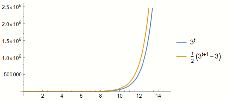
Figure 7: The Function of $E_{t}=3^{t}$ and $N_{t}=\frac{3^{t+1}-3}{2}$
Step 1: Initialization. Set $t=0$ , $G_{1}$ is a complete graph of order $\ell$ , and thus $N_{1}=\ell$ and $E_{1}=\binom{\ell}{2}$ . Set $G_{1}=S(1,\ell)$ .
Step 2: Generation of $G_{t+1}$ from $G_{t}$ . Let $S^{1}(t,\ell),S^{2}(t,\ell),\ldots,S^{\ell}(t,\ell)$ be all Sierpiński graphs added at Step $t$ , where $S^{i}(t,\ell)\cong S(t,\ell)$ ( $1\leq i\leq\ell$ ). At Step $t+1$ , we add one edge (bridge edge) between $S^{i}(t,\ell)$ and $S^{j}(t,\ell)$ , $i\neq j$ , namely the edge between vertices $\langle ij\cdots j\rangle$ and $\langle ji\cdots i\rangle$ .
For Sierpiński graphs $G_{t}=S(t,\ell)$ , its order and size are $N_{t}=\ell^{t}$ and $E_{t}=\frac{\ell^{t+1}-\ell}{2}$ , respectively; see Table 2 and Figure 7 (for $\ell=3$ ).
Table 2: The size and order of $G_{t}$ for $\ell=3$
| $t$ | 1 | 2 | 3 | 4 | 5 | 6 | t |
| --- | --- | --- | --- | --- | --- | --- | --- |
| $N_{t}$ | 3 | 9 | 27 | 81 | 242 | 729 | $\ell^{t}$ |
| $E_{t}$ | 3 | 12 | 39 | 120 | 363 | 1092 | $\frac{\ell^{t+1}-\ell}{2}$ |
The degree distribution for $t$ times are
$$
\left(\underbrace{\ell-1,\ell-1,\cdots,\ell-1}_{\ell},\underbrace{\ell,\ell,
\ell,\cdots,\ell}_{\ell^{t}-\ell}\right). \tag{11}
$$
From Equation 11, the instantaneous degree distribution is $P(\ell-1,t)=1/\ell^{t-1}$ for $t=2,\cdots,T$ and $P(\ell,t)=(\ell^{t}-\ell)/\ell^{t}$ for $t=2,\cdots,T$ . Note that the density of Sierpiński graphs is $\rho=E_{t}/\binom{N_{t}}{2}\rightarrow 0$ for $t\rightarrow+\infty$ . For large enough $\ell$ and any $1\leq k\leq\ell$ , we have $|\{v\in V(G)|d_{S(t,\ell)}(v)|\geq k\}\approx|V(S(t,\ell))|$ .
**Theorem 3.1**
*[11] If $n\in\mathbb{N}$ and $G$ is a graph, then $\kappa\left(S(n,G)\right)=\kappa(G)$ and $\lambda\left(S(n,G)\right)=\lambda(G)$ .*
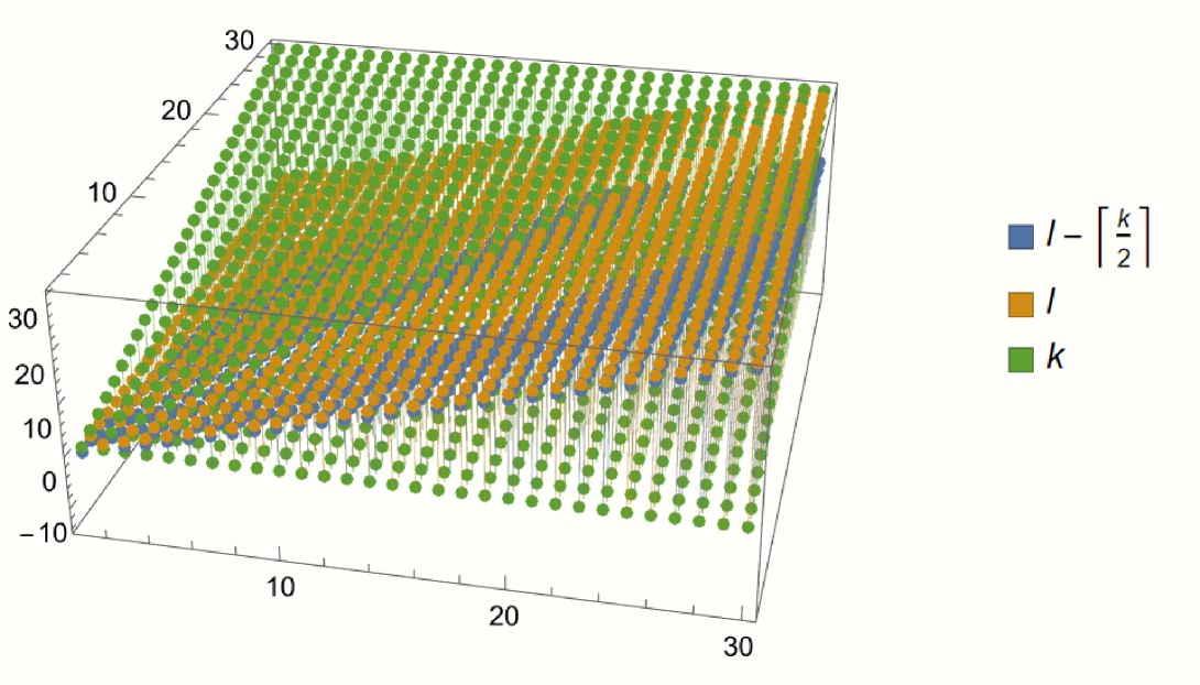
From Theorem 3.1, we have $\kappa\left(S(n,\ell)\right)=\kappa(K_{\ell})=\ell-1$ and $\lambda\left(S(n,\ell)\right)=\lambda(K_{\ell})=\ell-1$ . Note that $\lambda_{k}(S(n,\ell))=\ell-\left\lceil k/2\right\rceil$ and $\kappa_{k}(S(n,\ell))=\ell-\left\lceil k/2\right\rceil$ ; see Figure 8.
<details>
<summary>x4.png Details</summary>
### Visual Description
## 3D Scatter Plot: Mathematical Relationship Visualization
### Overview
The image displays a 3D scatter plot containing three distinct data series, represented by colored spheres (blue, orange, and green). The plot visualizes the relationship between three variables, likely representing indices or parameters ($l$ and $k$). The data points are arranged in a grid-like structure, forming three distinct, parallel, sloping planes within a 3D coordinate system.
### Components/Axes
* **Vertical Axis (Z-axis):** Ranges from -10 to 30, with major tick marks at -10, 0, 10, 20, and 30.
* **Horizontal Axis (X-axis):** Ranges from 0 to 30, with major tick marks at 10, 20, and 30.
* **Depth Axis (Y-axis):** Ranges from 0 to 30, with major tick marks at 10, 20, and 30.
* **Legend (Positioned on the right):**
* **Blue Square:** $l - [k/2]$
* **Orange Square:** $l$
* **Green Square:** $k$
### Detailed Analysis
The plot is composed of three distinct data series, each forming a planar surface in 3D space.
* **Green Series ($k$):**
* **Visual Trend:** This series forms the highest plane. It slopes upward consistently as both the X and Y coordinates increase.
* **Data Points:** At the furthest extent of the axes (near 30, 30), the green points reach the Z=30 level. Near the origin, the values are close to 0.
* **Orange Series ($l$):**
* **Visual Trend:** This series forms the middle plane. It is parallel to the green plane but consistently offset downwards.
* **Data Points:** The orange points track slightly below the green points across the entire grid.
* **Blue Series ($l - [k/2]$):**
* **Visual Trend:** This series forms the lowest plane. It is significantly offset below the orange plane.
* **Data Points:** The vertical distance between the blue plane and the orange plane increases as the value of $k$ increases, consistent with the subtraction of $[k/2]$.
### Key Observations
* **Parallelism:** All three data series form parallel planes, indicating a linear relationship between the variables.
* **Spacing:** The vertical gap between the Green ($k$) and Orange ($l$) series appears constant. The gap between the Orange ($l$) and Blue ($l - [k/2]$) series increases as $k$ increases, which is visually consistent with the mathematical definition provided in the legend.
* **Density:** The points are distributed in a uniform grid pattern across the X-Y plane, suggesting a systematic sampling of the variables $l$ and $k$.
### Interpretation
This visualization represents a mathematical function or algorithm, likely related to computer science indexing or array manipulation.
* **Mathematical Meaning:** The plot demonstrates the behavior of three functions: $f(k) = k$, $f(l) = l$, and $f(l, k) = l - \lfloor k/2 \rfloor$. The use of square brackets $[k/2]$ in the legend strongly suggests integer division or a floor function, which is common in algorithms involving binary trees, heaps, or specific array partitioning schemes.
* **Relationship:** The green series ($k$) acts as the primary independent variable influencing the vertical position of the blue series. The orange series ($l$) acts as a baseline.
* **Peircean Investigative Note:** The visual "stepping" or separation of the planes confirms that the blue series is a transformation of the other two. The fact that the blue plane is the lowest and has the steepest relative drop-off as $k$ increases confirms the subtractive nature of the $[k/2]$ term. This is likely a visualization of how an index $l$ is modified by a parameter $k$ in a specific computational context.
</details>
Figure 8: The generalized (edge-)connectivity of $S(n,\ell)$
The number of spanning tree of $G$ denoted by $\tau(G)$ . Let
$$
\rho(G)=\lim_{V(G)\longrightarrow\infty}\frac{\ln|\tau(G)|}{\left|V(G)\right|}, \tag{12}
$$
where $\rho(G)$ is called the entropy of spanning trees or the asymptotic complexity [2, 7].
As an application of generalized (edge-)connectivity, similarly to the Equation 12, it can describe the fault tolerance of a graph or network, a common metric is called the entropy of spanning trees.
we give the entropy of the $k$ -Steiner tree of a graph $G$ can be defined as
$$
\rho_{k}(G)=\lim_{|V(G)|\longrightarrow\infty}\frac{\ln|\kappa_{k}(G)|}{\left|
V(G)\right|}
$$
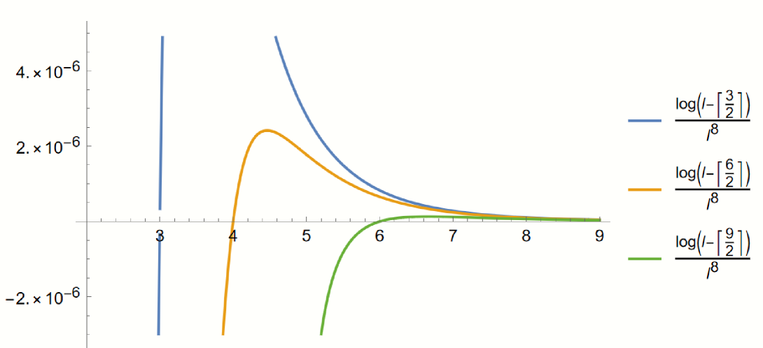
The entropy of the $3,6,9$ -Steiner tree of Sierpiński graph $S(8,\ell)$ can be seen in Figure 9.
<details>
<summary>x5.png Details</summary>
### Visual Description
## Mathematical Plot: Logarithmic Function Analysis
### Overview
The image displays a mathematical plot featuring three distinct curves, each representing a variation of a logarithmic function divided by a power function. The plot is set against a white background with a standard Cartesian coordinate system. The x-axis ranges from 3 to 9, and the y-axis ranges from approximately $-2 \times 10^{-6}$ to $4 \times 10^{-6}$.
### Components/Axes
* **X-Axis:** Represents the variable $l$. The scale is linear, marked with integers from 3 to 9.
* **Y-Axis:** Represents the output value of the functions. The scale is in scientific notation, with major ticks at $-2 \times 10^{-6}$, $0$, $2 \times 10^{-6}$, and $4 \times 10^{-6}$.
* **Legend (Right side):** Lists the three functions plotted, color-coded to match the lines:
* **Blue Line:** $\frac{\log(l - [\frac{3}{2}])}{l^8}$
* **Orange Line:** $\frac{\log(l - [\frac{6}{2}])}{l^8}$
* **Green Line:** $\frac{\log(l - [\frac{9}{2}])}{l^8}$
*(Note: The variable $l$ is used in the expressions. The brackets $[\dots]$ denote the grouping of the fraction.)*
</details>
Figure 9: Entropy of $S(n,\ell)$ for $n=8$ , $k=3,6,9$ and $\ell\rightarrow+\infty$
The definition of clustering coefficient can be found in [3]. Let $N_{v}(t)$ be the number of edges in $G_{t}$ among neighbors of $v$ , which is the number of triangles connected to the vertex $v$ . The clustering coefficient of a graph is based on a local clustering coefficient for each vertex
$$
C[v]=\frac{N_{v}(t)}{d_{G}(v)(d_{G}(v)-1)/2},
$$
If the degree of node $v$ is $0 0$ or $1$ , then we can set $C[v]=0$ . By definition, we have $0\leq C[v]\leq 1$ for $v\in V(G)$ .
The clustering coefficient for the whole graph $G$ is the average of the local values $C(v)$
$$
C(G)=\frac{1}{|V(G)|}\left(\sum_{v\in V(G)}C[v]\right).
$$
The clustering coefficient of a graph is closely related to the transitivity of a graph, as both measure the relative frequency of triangles [22, 24].
**Proposition 3.1**
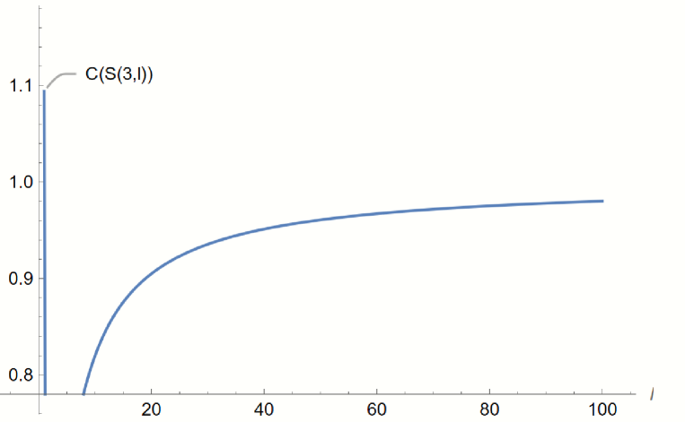
*The clustering coefficient of generalized Sierpiński graph $S(n,\ell)$ is
$$
C(S(n,\ell))=\frac{\ell^{-n}\left(2\ell-2\ell^{n}+\ell^{n+1}\right)}{\ell}.
$$*
* Proof*
For any $v\in V(S(n,\ell))$ , if $v$ is a extremal vertex, then $d_{S(n,\ell)}(v)=\ell-1$ and $G[\{N(v)\}]\cong K_{\ell-1}$ , and hence
$$
C[v]=\frac{N_{v}(t)}{d_{G}(v)(d_{G}(v)-1)/2}={\binom{\ell-1}{2}}/{\binom{\ell-
1}{2}}=1.
$$
If $v$ is not a extremal vertex, then $d_{S(n,\ell)}(v)=\ell$ and $G[\{N(v)\}]\cong K_{\ell}+e$ , where $K_{\ell}+e$ is graph obtained from a complete graph $K_{\ell}$ by adding a pendent edge. Hence, we have $C[v]={\binom{\ell-1}{2}}/{\binom{\ell}{2}}=\frac{\ell-2}{\ell}$ . Since there exists $\ell$ extremal vertices in Sierpiński graph $S(n,\ell)$ , it follows that
$$
C(S(n,\ell))=\frac{1}{|V(G)|}\left(\sum_{v\in V(G)}C[v]\right)=\frac{1}{\ell^{
n}}\left({\ell\times 1+(\ell^{n}-\ell)\frac{\ell-2}{\ell}}\right)=\frac{\ell^{
-n}\left(2\ell-2\ell^{n}+\ell^{n+1}\right)}{\ell}
$$
∎
<details>
<summary>x6.png Details</summary>
### Visual Description
## Line Chart: Mathematical Function Plot C(S(3,l))
### Overview
The image displays a single, continuous blue curve plotted on a Cartesian coordinate system. The curve represents a mathematical function labeled "C(S(3,l))". The plot illustrates a relationship where the output value increases as the input variable "l" increases, characterized by a diminishing rate of growth.
### Components/Axes
* **Y-Axis (Vertical):** Represents the output value of the function. The scale is marked with the values 0.8, 0.9, 1.0, and 1.1.
* **X-Axis (Horizontal):** Represents the variable "l" (lowercase L). The scale is marked with the values 20, 40, 60, 80, and 100.
* **Data Series:** A single, solid blue line representing the function C(S(3,l)).
* **Annotation:** A callout label "C(S(3,l))" is positioned in the upper-left area, with a line pointing to the curve.
### Detailed Analysis
The curve exhibits a monotonic increasing trend with a concave-down shape, indicating diminishing marginal returns.
**Approximate Data Points (x, y):**
* **x ≈ 10:** y ≈ 0.80
* **x ≈ 20:** y ≈ 0.90
* **x ≈ 40:** y ≈ 0.94
* **x ≈ 60:** y ≈ 0.96
* **x ≈ 80:** y ≈ 0.97
* **x ≈ 100:** y ≈ 0.98
*Note: The curve starts near the x-axis origin (x ≈ 5) and rises sharply before flattening out as it approaches a horizontal asymptote slightly below 1.0.*
### Key Observations
* **Diminishing Returns:** The slope of the curve is steepest at the lowest values of "l" (between 5 and 20) and becomes progressively flatter as "l" increases toward 100.
* **Asymptotic Behavior:** The curve appears to be approaching a horizontal asymptote, likely at y = 1.0, though it does not reach or cross this value within the visible range of the plot.
* **Function Notation:** The label "C(S(3,l))" implies a nested function where "S" is a function of 3 and "l", and "C" is a function of that result.
### Interpretation
This plot represents a classic "saturation" or "diminishing returns" model.
* **What the data demonstrates:** As the input variable "l" increases, the output of the function C(S(3,l)) increases, but the incremental gain for each additional unit of "l" decreases.
* **Why it matters:** In technical or scientific contexts, this type of curve is common when modeling efficiency, probability, or resource utilization. For example, if "l" represents a resource (like time, length, or energy) and "C" represents a performance metric, the system reaches a point of diminishing returns where adding more resources yields negligible improvements.
* **Reading between the lines:** The fact that the curve approaches 1.0 suggests that 1.0 may represent a theoretical maximum, such as 100% efficiency, full probability, or a normalized capacity limit. The fixed parameter "3" suggests that this is one specific instance of a family of curves; changing the "3" to a different value would likely shift the curve's steepness or the location of the asymptote.
</details>
Figure 10: The Function of $C_{S(3,l)}$
<details>
<summary>x7.png Details</summary>
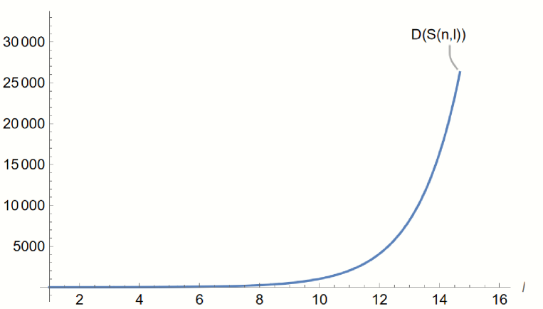
### Visual Description
## Line Chart: Mathematical Plot of $D(S(n,l))$
### Overview
The image displays a single, continuous mathematical plot representing the function $D(S(n,l))$ as a function of the variable $l$. The plot illustrates a rapid, non-linear increase in value as $l$ increases, characteristic of exponential or combinatorial growth.
### Components/Axes
* **Y-Axis (Vertical):** Represents the output value of the function $D(S(n,l))$. The scale ranges from 0 to 30,000, with major tick marks at intervals of 5,000 (0, 5000, 10000, 15000, 20000, 25000, 30000).
* **X-Axis (Horizontal):** Represents the variable $l$. The scale ranges from 2 to 16, with major tick marks at intervals of 2 (2, 4, 6, 8, 10, 12, 14, 16).
* **Data Series:** A single, solid blue line representing the function $D(S(n,l))$.
* **Annotation:** A text label "$D(S(n,l))$" is positioned in the upper-right quadrant, with a leader line pointing to the terminus of the blue curve.
### Detailed Analysis
**Trend Verification:**
The curve exhibits a "hockey stick" growth pattern.
* **Initial Phase ($l = 2$ to $l \approx 8$):** The curve is nearly horizontal, remaining very close to the x-axis (y-values near 0).
* **Transition Phase ($l \approx 8$ to $l \approx 10$):** The curve begins to slope upward, indicating the onset of accelerated growth.
* **Explosive Phase ($l \approx 10$ to $l \approx 14.8$):** The slope increases dramatically, indicating super-linear or exponential growth.
**Data Point Approximations:**
* At $l = 8$: The value is approximately 500.
* At $l = 10$: The value is approximately 1,500 to 2,000.
* At $l = 12$: The value is approximately 6,000 to 7,000.
* At $l = 14$: The value is approximately 20,000.
* At $l \approx 14.8$ (terminus): The value is approximately 26,000 to 27,000.
### Key Observations
* **Non-Linearity:** The function is clearly non-linear. The rate of change (derivative) increases significantly as $l$ increases.
* **Abrupt Termination:** The curve ends abruptly at $l \approx 14.8$. This suggests either a computational limit (the calculation was stopped) or a physical constraint on the system being modeled.
* **Notation:** The notation $S(n,l)$ is standard in computer science and combinatorics, often representing a search space of size $n$ with length $l$.
### Interpretation
The data demonstrates a classic case of **combinatorial explosion**.
* **What the data suggests:** The function $D(S(n,l))$ likely represents a metric of complexity, such as the number of states to explore, the number of operations required, or the size of a search tree. The visual evidence shows that for small values of $l$ (below 8), the problem is computationally trivial. However, as $l$ approaches 15, the "cost" or "size" of the function grows so rapidly that it likely becomes computationally intractable.
* **Why it matters:** This type of graph is frequently used in technical documentation to justify the need for heuristics, approximation algorithms, or pruning techniques in search algorithms. It visually communicates the "wall" that developers hit when scaling systems that rely on exhaustive search or brute-force methods.
* **Peircean Investigative Note:** The abrupt termination of the line at $l \approx 14.8$ is a significant anomaly. It implies that the system generating this plot likely encountered a memory overflow, a timeout, or a hard-coded limit in the simulation software, rather than the function naturally ending. The graph is a warning of the limitations of the underlying algorithm.
</details>
Figure 11: The diameter of $S(n,\ell)$
**Theorem 3.2**
*[21] The diameter of $S(n,\ell)$ is $Diam(S(n,\ell))=2^{\ell}-1$ ;*
For network properties of Sierpiński graph $S(n,\ell)$ , the the diameter function can be seen in Figure 11 and its clustering coefficient is closely related to $1$ when $\ell\longrightarrow\infty$ ; see Figure 11, which implies that the Sierpiński graph $S(n,\ell)$ is a hight transitivity graph.
## 4 Acknowledgments
The authors would like to thank the anonymous referee for the careful reading of the manuscript and the numerous helpful suggestions and comments.
## References
- [1] J.A. Bondy, U.S.R. Murty, Graph Theory, GTM 244, Springer, 2008.
- [2] R. Burton, R. Pemantle, Local characteristics, entropy and limit theorems for spanning trees and domino tilings via transfer-impedances, Ann. Prob. 21 (1993), 1329–1371.
- [3] B. Bollobás, O.M. Riordan, Mathematical results on scale-free random graphs, in: S. Bornholdt, H.G. Schuster (Eds.), Handbook of Graphs and Networks: From the Genome to the Internet, Wiley-VCH, Berlin, 2003, 1–34.
- [4] G. Chartrand, F. Okamoto, P. Zhang, Rainbow trees in graphs and generalized connectivity, Networks 55(4) (2010), 360–367.
- [5] B.L. Chen, K.C. Huange, On the Line $k$ -arboricity of $K_{n}$ and $K_{n,n}$ , Discrete Math. 254 (2002), 83–87.
- [6] X. Cheng, D. Du, Steiner trees in Industry, Kluwer Academic Publisher, Dordrecht, 2001.
- [7] M. Dehmer, F. Emmert-Streib, Z. Chen, X. Li, and Y. Shi, Mathematical foundations and applications of graph entropy, John Wiley $\&$ Sons. (2017).
- [8] D. Du, X. Hu, Steiner tree problems in computer communication networks, World Scientific, 2008.
- [9] C. Hao, W. Yang, The generalized connectivity of data center networks. Parall. Proce. Lett. 29 (2019), 1950007.
- [10] J. Gu, J. Fan, Q. Ye, L. Xi, Mean geodesic distance of the level- $n$ Sierpiński gasket, J. Math. Anal. Appl. 508(1) (2022), 125853.
- [11] S. Klavžar, U. Milutinović, Graphs $S(n,k)$ and a variant of tower of hanoi problem, Czechoslovak Math. J. 122(47) (1997), 95–104.
- [12] H. Li, X. Li, and Y. Sun, The generalied $3$ -connectivity of Cartesian product graphs, Discrete Math. Theor. Comput. Sci. 14(1) (2012), 43–54.
- [13] H. Li, Y. Ma, W. Yang, Y. Wang, The generalized $3$ -connectivity of graph products, Appl. Math. Comput. 295 (2017), 77–83.
- [14] S. Li, J. Tu, C. Yu, The generalized $3$ -connectivity of star graphs and bubble-sort graphs, Appl. Math. Comput. 274(1) (2016), 41–46.
- [15] X. Li, Y. Mao, Generalized Connectivity of Graphs, Springer Briefs in Mathematics, Springer, Switzerland, 2016.
- [16] X. Li, Y. Mao, Y. Sun, On the generalized (edge-)connectivity of graphs, Australasian J. Combin. 58(2) (2014), 304–319.
- [17] Y. Li, Y. Mao, Z. Wang, Z. Wei, Generalized connectivity of some total graphs, Czechoslovak Math. J. 71 (2021), 623–640.
- [18] C. Li, S. Lin, S. Li, The $4$ -set tree connectivity of $(n,k)$ -star networks, Theor. Comput. Sci. 844 (2020), 81–86.
- [19] S. Lin, Q. Zhang, The generalized $4$ -connectivity of hypercubes. Discrete Appl. Math. 220 (2017), 60–67.
- [20] H. Li, X. Li, Y. Sun, The generalized $3$ -connectivity of Cartesian product graphs, Discrete Math. Theor. Comput. Sci. 14 (2012), 43–54.
- [21] D. Parisse, On some metric properties of the the Sierpiński graphs $S(n,\ell)$ , Ars Comb. 90 (2009), 145–160.
- [22] J. Reichardt, Structure in complex networks. Springer Science $\&$ Business Media, 2008.
- [23] A. Sahu, A. Priyadarshi, On the box-counting dimension of graphs of harmonic functions on the Sierpiński gasket. J. Math. Analy. Appl. 487(2) (2020), 124036.
- [24] X. Wang, X. LI, G. R.Chen, Introduction to Network Science. Beijing: Higher Education Press, 2012.
- [25] B. Xue, L. Zuo, G. Li, The hamiltonicity and path $t$ -coloring of Sierpiński-like graphs, Discrete Appl. Math. 160 (2012), 1822–836.
- [26] B. Xue, L. Zuo, On the linear $(n-1)$ -arboricity of $K_{n}$ , Discrete Appl. Math. 158 (2010) 1546–1550.
- [27] S. Zhao, R. Hao, L. Wu, The generalized connectivity of $(n,k)$ -bubble-sort graphs. The Comput. J. 62 (2019), 1277–1283.
- [28] S. Zhao, R. Hao, J. Wu, The generalized $3$ -connectivity of some regular networks, J. Parall. Distr. Comput. 133 (2019), 18–29.
- [29] S. Zhao, R. Hao, The generalized connectivity of alternating group graphs and $(n,k)$ -star graphs, Discrete Appl. Math. 251 (2018), 310–321.
- [30] S. Zhao, R. Hao, E. Cheng, Two kinds of generalized connectivity of dual cubes, Discrete Appl. Math. 257 (2019), 306–316.
- [31] S. Zhao, R. Hao, The generalized connectivity of alternating group graphs and $(n,k)$ -star graphs, Discrete Appl. Math. 251 (2018), 310–321.
- [32] S. Zhao, R. Hao, The generalized $4$ -connectivity of exchanged hypercubes, Applied Mathe. Comput. 347 (2019), 342–353.
- [33] S. Zhao, R. Hao, J. Wu, The generalized $4$ -connectivity of hierarchical cubic networks, Discrete Appl. Mathe., 289 (2021), 194–206.
- [34] S. Zhao, J. Chang, Z. Li, The generalized $4$ -connectivity of pancake graphs, Discrete Appl. Math. 327 (2023), 77–86.
- [35] S. Zhao, R. Hao, The generalized $4$ -connectivity of exchanged hypercubes. Appl. Math. Comput. 347 (2019), 342–353.