# Constructing Disjoint Steiner Trees in Sierpiński Graphs††thanks: Supported by the National Natural Science Foundation of China (Nos. 12201375, 12471329 and 12061059) and the Qinghai Key Laboratory of Internet of Things Project (2017-ZJ-Y21).
**Authors**:
- Chenxu Yang (School of Computer)
- Qinghai Normal University
- Xining
- Qinghai
- Ping Li (School of Mathematics and Statistics)
- Shaanxi Normal University
- Xi’an
- Shaanxi
- Yaping Mao
- Xining
- Qinghai
- Eddie Cheng (Department of Mathematics)
- Oakland University
- Rochester
- MI USA
- Ralf Klasing
- Université de Bordeaux
- Bordeaux INP
- CNRS
- LaBRI
- UMR
- Talence
> Corresponding author.
25 2 10.46298/fi.12478
## Abstract
Let $G$ be a graph and $S\subseteq V(G)$ with $|S|\geq 2$ . Then the trees $T_{1},T_{2},\cdots,T_{\ell}$ in $G$ connecting $S$ are internally disjoint Steiner trees (or $S$ -Steiner trees) if $E(T_{i})\cap E(T_{j})=\emptyset$ and $V(T_{i})\cap V(T_{j})=S$ for every pair of distinct integers $1\leq i,j\leq\ell$ . Similarly, if we only have the condition $E(T_{i})\cap E(T_{j})=\emptyset$ but without the condition $V(T_{i})\cap V(T_{j})=S$ , then they are edge-disjoint Steiner trees $S$ -Steiner trees. The generalized $k$ -connectivity, denoted by $\kappa_{k}(G)$ , of a graph $G$ , is defined as $\kappa_{k}(G)=\min\{\kappa_{G}(S)|S\subseteq V(G)\ \textrm{and}\ |S|=k\}$ , where $\kappa_{G}(S)$ is the maximum number of internally disjoint $S$ -Steiner trees. The generalized $k$ -edge-connectivity $\lambda_{k}(G)$ of $G$ is defined as $\lambda_{k}(G)=\min\{\lambda_{G}(S)\,|\,S\subseteq V(G)\ and\ |S|=k\}$ , where $\lambda_{G}(S)$ is the maximum number of edge-disjoint Steiner trees connecting $S$ in $G$ . These concepts are generalizations of the concepts of connectivity and edge-connectivity, and they can be used as measures of vulnerability of networks. It is, in general, difficult to compute these generalized connectivities. However, there are precise results for some special classes of graphs. In this paper, we obtain the exact value of $\lambda_{k}(S(n,\ell))$ for $3\leq k\leq\ell^{n}$ , and the exact value of $\kappa_{k}(S(n,\ell))$ for $3\leq k\leq\ell$ , where $S(n,\ell)$ is the Sierpiński graphs with order $\ell^{n}$ . As a direct consequence, these graphs provide additional interesting examples when $\lambda_{k}(S(n,\ell))=\kappa_{k}(S(n,\ell))$ . We also study the some network properties of Sierpiński graphs. Keywords: Steiner Tree; Generalized Connectivity; Sierpiński Graph. AMS subject classification 2010: 05C40, 05C85.
volume: 194 issue: 1
Constructing disjoint Steiner trees in Sierpiński graphs
## 1 Introduction
All graphs considered in this paper are undirected, finite and simple. We refer the readers to [1] for graph theoretical notation and terminology not described here. For a graph $G$ , let $V(G)$ and $E(G)$ denote the set of vertices and the set of edges of $G$ , respectively. The neighborhood set of a vertex $v\in V(G)$ is $N_{G}(v)=\{u\in V(G)\,|\,uv\in E(G)\}$ . The degree of a vertex $v$ in $G$ is denoted by $d(v)=|N_{G}(v)|$ . Denote by $\delta(G)$ ( $\Delta(G)$ ) the minimum degree (maximum degree) of the graph $G$ . For a vertex subset $S\subseteq V(G)$ , the subgraph induced by $S$ in $G$ is denoted by $G[S]$ and similarly $G[V\setminus S]$ for $G\setminus S$ or $G-S$ . Especially, $G-v$ is $G[V\setminus\{v\}]$ . Let $\overline{G}$ be the complement of $G$ . For a partition $\mathcal{P}=\{V_{1},V_{2},\ldots,V_{t}\}$ of $V(G)$ , let $G/\mathcal{P}$ be the graph obtained from $G$ by deleting $\bigcup_{i\in[t]}E(G[V_{i}])$ and then identifying each $V_{i}$ , respectively. For any positive integers $n$ , we always use the convenient notation $[n]$ to denote the set $\{1,2,\cdots,n\}$ .
### 1.1 Generalized (edge-)connectivity
Connectivity and edge-connectivity are two of the most basic concepts of graph-theoretic measures. Such concepts can be generalized, see, for example, [16]. For a graph $G=(V,E)$ and a set $S\subseteq V(G)$ of at least two vertices, an $S$ -Steiner tree or a Steiner tree connecting $S$ (or simply, an $S$ -tree) is a subgraph $T=(V^{\prime},E^{\prime})$ of $G$ that is a tree with $S\subseteq V^{\prime}$ . Note that when $|S|=2$ a minimal $S$ -Steiner tree is just a path connecting the two vertices of $S$ .
Let $G$ be a graph and $S\subseteq V(G)$ with $|S|\geq 2$ . Then the trees $T_{1},T_{2},\cdots,T_{\ell}$ in $G$ are internally disjoint $S$ -trees if $E(T_{i})\cap E(T_{j})=\emptyset$ and $V(T_{i})\cap V(T_{j})=S$ for every pair of distinct integers $i,j$ , $1\leq i,j\leq\ell$ . Similarly, if we only have the condition $E(T_{i})\cap E(T_{j})=\emptyset$ but without the condition $V(T_{i})\cap V(T_{j})=S$ , then they are edge-disjoint $S$ -trees (Note that while we do not have the condition $V(T_{i})\cap V(T_{j})=S$ , it is still true that $S\subseteq V(T_{i})\cap V(T_{j})$ as $T_{i}$ and $T_{j}$ are $S$ -trees.) The generalized $k$ -connectivity, denoted by $\kappa_{k}(G)$ , of a graph $G$ , is defined as $\kappa_{k}(G)=\min\{\kappa_{G}(S)|S\subseteq V(G)\ \textrm{and}\ |S|=k\}$ , where $\kappa_{G}(S)$ is the maximum number of internally disjoint $S$ -trees. The generalized local edge-connectivity $\lambda_{G}(S)$ is the maximum number of edge-disjoint $S$ -trees in $G$ . The generalized $k$ -edge-connectivity $\lambda_{k}(G)$ of $G$ is defined as $\lambda_{k}(G)=\min\{\lambda_{G}(S)\,|\,S\subseteq V(G)\ and\ |S|=k\}$ . Since internally disjoint $S$ -trees are edge-disjoint but not vice versa, it follows from the definitions that $\kappa_{k}(G)\leq\lambda_{k}(G)$ . There are many results on generalized (edge-)connectivity; see the book [15] by Li and Mao.
For a graph $G$ and two distinct vertices $x,y$ of $G$ , the local connectivity $p_{G}(x,y)$ of $x$ and $y$ is defined as the maximum number of pairwise internally disjoint paths between $x$ and $y$ , and the local edge-connectivity $\lambda_{G}(x,y)$ is defined as the maximum number of pairwise edge-disjoint paths between $x$ and $y$ . The connectivity of $G$ is defined as $\kappa(G)=\min\{p_{G}(x,y)\,|\,x,y\in V(G),\,x\neq y\}$ , and the edge-connectivity of $G$ is defined as $\lambda(G)=\min\{\lambda_{G}(x,y)\,|\,x,y\in V(G),\,x\neq y\}$ . It is clear that when $|S|=2$ , $\lambda_{2}(G)$ is just the standard edge-connectivity $\lambda(G)$ of $G$ , $\kappa_{2}(G)=\kappa(G)$ , that is, the standard connectivity of $G$ . Thus $\kappa_{k}(G)$ and $\lambda_{k}(G)$ are the generalized connectivity of $G$ and the generalized edge-connectivity of $G$ , respectively.
As it is well-known, for any graph $G$ , we have polynomial-time algorithms to find the classical connectivity $\kappa(G)$ and edge-connectivity $\lambda(G)$ . Given two fixed positive integers $k$ and $\ell$ , for any graph $G$ the problem of deciding whether $\lambda_{k}(G)\geq\ell$ can be solved by a polynomial-time algorithm. If $k\ (k\geq 3)$ is a fixed integer and $\ell\ (\ell\geq 2)$ is an arbitrary positive integer, the problem of deciding whether $\kappa(S)\geq\ell$ is $NP$ -complete. For any fixed integer $\ell\geq 3$ , given a graph $G$ and a subset $S$ of $V(G)$ , deciding whether there are $\ell$ internally disjoint Steiner trees connecting $S$ , namely deciding whether $\kappa(S)\geq\ell$ , is $NP$ -complete. For more details on the computational complexity of generalized connectivity and generalized edge-connectivity, we refer to the book [15].
In addition to being a natural combinatorial measure, generalized $k$ -connectivity can be motivated by its interesting interpretation in practice. For example, suppose that $G$ represents a network. If one wants to “connect” a pair of vertices of $G$ “minimally”, then a path is used to “connect” them. More generally, if one wants to “connect” a set $S$ of vertices of $G$ , with $|S|\geq 3$ , “minimally”, then it is desirable to use a tree to “connect” them. Such trees are precisely $S$ -trees, which are also used in computer communication networks (see [8]) and optical wireless communication networks (see [6]).
From a theoretical perspective, generalized edge-connectivity is related to Nash-Williams-Tutte theorem and Menger theorem; see [15]. The generalized edge-connectivity has applications in $VLSI$ circuit design. In this application, a Steiner tree is needed to share an electronic signal by a set of terminal nodes. Another application, which is our primary focus, arises in the Internet Domain. Imagine that a given graph $G$ represents a network. We arbitrarily choose $k$ vertices as nodes. Suppose one of the nodes in $G$ is a broadcaster, and all other nodes are either users or routers (also called switches). The broadcaster wants to broadcast as many streams of movies as possible, so that the users have the maximum number of choices. Each stream of movie is broadcasted via a tree connecting all the users and the broadcaster. So, in essence we need to find the maximum number Steiner trees connecting all the users and the broadcaster, namely, we want to get $\lambda(S)$ , where $S$ is the set of the $k$ nodes. Clearly, it is a Steiner tree packing problem. Furthermore, if we want to know whether for any $k$ nodes the network $G$ has above properties, then we need to compute $\lambda_{k}(G)=\min\{\lambda(S)\}$ in order to prescribe the reliability and the security of the network. For more details, we refer to the book [15].
### 1.2 Sierpiński graphs
In 1997, Klavžar and Milutinović introduced the concept of Sierpiński graph $S(n,\ell)$ in [11]. We denote $n$ -tuples $V^{n}$ by the set
$$
V^{n}=\{\langle u_{0}u_{1}\cdots u_{n-1}\rangle|\ u_{i}\in\{0,1,\ldots,\ell-1
\}\textrm{ and }i\in\{0,1,\ldots,n-1\}\}.
$$
A word $u$ of size $n$ are denoted by $\langle u_{0}u_{1},\cdots,u_{n-1}\rangle$ in which $u_{i}\in\{0,\ldots,\ell-1\}$ . The concatenation of two words $u=\langle u_{0}u_{1}\cdots u_{n-1}\rangle$ and $v=\langle v_{0}v_{1}\cdots v_{n-1}\rangle$ is denoted by $uv$ .
**Definition 1**
*The Sierpiński graph $S(n,\ell)$ is defined as below, for $n\geq 1$ and $\ell\geq 3$ , the vertex set of $S(n,\ell)$ consists of all $n$ -tuples of integers $0,1,\cdots,\ell-1$ . That is, $V(S(n,\ell))=V^{n}$ , where $uv=(u_{0}u_{1}\cdots u_{n-1},v_{0}v_{1}\cdots v_{n-1})$ is an edge of $E(S(n,\ell))$ if and only if there exists $d\in\{0,1,\ldots,\ell-1\}$ such that: $(1)$ $u_{j}=v_{j}$ , if $j<d$ ; $(2)$ $u_{d}\neq v_{d}$ ; $(3)$ $u_{j}=v_{d}$ and $v_{j}=u_{d}$ , if $j>d$ .*
<details>
<summary>x1.png Details</summary>
### Visual Description
## Diagram: Network Graph with Numbered Nodes
### Overview
The image displays a directed or undirected graph diagram consisting of 16 circular nodes, each labeled with a unique two-digit number. The nodes are interconnected by straight lines (edges), forming a complex, symmetrical network structure. The layout is hierarchical and geometric, with a central vertical spine and two lateral clusters.
### Components/Axes
* **Nodes:** 16 white circles, each containing a two-digit numerical label.
* **Edges:** Straight black lines connecting the nodes.
* **Labels:** All text consists of the two-digit numbers within or adjacent to the nodes.
* **Spatial Layout:** The graph is arranged with a clear vertical axis of symmetry. It features a central column, a top triangular formation, and two mirrored triangular clusters on the lower left and right.
### Detailed Analysis
**Node Inventory and Connections:**
The nodes can be grouped by their numerical prefix, suggesting a categorical or hierarchical organization.
* **Central Spine (0x & 1x series):**
* `00`: The bottom-most central node. Connected to `01`, `02`, `03`.
* `01`: Directly above `00`. Connected to `00`, `10`, `02`, `03`.
* `10`: Above `01`. Connected to `01`, `11`, `12`, `13`.
* `11`: Above `10`. Connected to `10`, `12`, `13`.
* `12` & `13`: The topmost nodes, forming a horizontal pair. Connected to each other, to `11`, to `10`, and to the lateral clusters (`12` to `21`; `13` to `31`).
* **Left Cluster (2x series):**
* `20`: Inner node of the left cluster. Connected to `02`, `21`, `22`, `23`.
* `21`: Outer-left node. Connected to `20`, `22`, `23`, and the top node `12`.
* `22`: Central node within the left cluster triangle. Connected to `20`, `21`, `23`.
* `23`: Bottom node of the left cluster. Connected to `20`, `21`, `22`, and the right cluster node `32`.
* **Right Cluster (3x series):**
* `30`: Inner node of the right cluster. Connected to `03`, `31`, `32`, `33`.
* `31`: Outer-right node. Connected to `30`, `32`, `33`, and the top node `13`.
* `32`: Bottom node of the right cluster. Connected to `30`, `31`, `33`, and the left cluster node `23`.
* `33`: Central node within the right cluster triangle. Connected to `30`, `31`, `32`.
* **Connecting Nodes:**
* `02`: Bridges the central spine (`00`, `01`) to the left cluster (`20`).
* `03`: Bridges the central spine (`00`, `01`) to the right cluster (`30`).
**Structural Flow:**
The graph exhibits a clear top-down and center-outward flow. The central spine (`00` to `11`) acts as a primary axis. The top nodes (`12`, `13`) connect down to the lateral clusters. The two lateral clusters (`2x` and `3x`) are themselves tightly interconnected internally and are linked to each other at their bases (`23`-`32` edge).
### Key Observations
1. **Symmetry:** The graph is almost perfectly symmetrical about the vertical axis running through nodes `00`, `01`, `10`, `11`.
2. **Hierarchical Grouping:** The first digit of the node labels (`0`, `1`, `2`, `3`) strongly correlates with spatial grouping: `0x`/`1x` are central/vertical, `2x` is left, `3x` is right.
3. **High Connectivity:** Most nodes have a degree (number of connections) of 3 or 4, indicating a robustly connected network. Nodes `01`, `10`, `20`, `21`, `30`, `31` appear to be key hubs.
4. **Triangular Motifs:** The structure is built from interconnected triangles (e.g., `11`-`12`-`13`, `20`-`21`-`22`, `30`-`31`-`33`), which are stable geometric forms.
### Interpretation
This diagram likely represents a **network topology, a system architecture, or a mathematical graph model**. The numbered nodes could symbolize servers, processors, data centers, logical units, or abstract states. The edges represent communication links, dependencies, or relationships.
The structure suggests a **distributed or federated system**. The central spine (`0x`, `1x`) could be a core control or routing layer. The lateral clusters (`2x`, `3x`) might represent separate regional or functional subsystems that are internally cohesive but also connected to the core and to each other (via the `23`-`32` link), enabling redundancy and cross-communication. The top-level connection between `12` and `13` and their links down to the clusters (`21`, `31`) provide an alternative, high-level pathway, possibly for load balancing or failover.
The numerical labeling scheme is systematic, implying an addressable system where the prefix denotes a zone or tier and the suffix denotes an individual unit within that zone. The overall design prioritizes **interconnectivity, symmetry, and hierarchical organization**, which are common principles in reliable network design, parallel computing architectures, or organizational models.
</details>
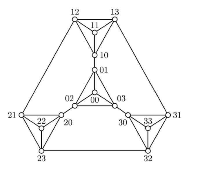
Figure 1: $S(2,4)$
Sierpiński graph $S(2,4)$ is shown in Figure 1. Note that $S(n,\ell)$ can be constructed recursively as follows: $S(1,\ell)$ is isomorphic to $K_{\ell}$ , which vertex set is 1-tuples set $\{0,\ldots,\ell-1\}$ . To construct $S(n,\ell)$ for $n>1$ , we take copies of $\ell$ times $S(n-1,\ell)$ and add the letter $i$ on the top of the vertices in $i$ -th copy of $S(n-1,\ell)$ , denoted by $S^{i}(n,\ell)$ . Note that there is exactly one edge (bridge edge) between $S^{i}(n,\ell)$ and $S^{j}(n,\ell)$ , $i\neq j$ , namely the edge between vertices $\langle ij\cdots j\rangle$ and $\langle ji\cdots i\rangle$ .
The vertices $(\underbrace{i,i,\cdots,i}_{n})$ , $i\in\{0,1,\ldots,\ell-1\}$ are the extreme vertices of $S(n,\ell)$ . Note that an extreme vertex $u$ of $S(n,\ell)$ has degree $d(u)=\ell-1$ . For $i\in\{0,\ldots,\ell-1\}$ and $n\geq 2$ , let $S^{i}(n-1,\ell)$ denote the subgraph of $S(n,\ell)$ induced by the vertices of the form $\{\langle iu_{1}\cdots u_{n-1}\rangle\,|\,0\leq u_{i}\leq\ell-1\}$ . The vertex set $V(S(n,\ell))$ can be partitioned into $\ell$ parts $V(S^{0}(n-1,\ell)),V(S^{1}(n-1,\ell)),\ldots,V(S^{\ell-1}(n-1,\ell))$ . For each $0\leq i\leq\ell-1$ , $S^{i}(n-1,\ell)$ is isomorphic to $S(n-1,\ell)$ . Note that $V(S(n,\ell))=V(S^{0}(n-1,\ell))\cup\cdots\cup V(S^{\ell-1}(n-1,\ell))$ and $S(n,\ell)$ is the graph obtained from $S^{0}(n-1,\ell),\ldots,S^{\ell-1}(n-1,\ell)$ by adding exactly one edge (bridge edge) between $S^{i}(n-1,\ell)$ and $S^{j}(n-1,\ell)$ , $i\neq j$ , and the bridge edge joins $\langle ij\cdots j\rangle$ and $\langle ji\cdots i\rangle$ (notices that $\langle ij\cdots j\rangle$ and $\langle ji\cdots i\rangle$ are extreme vertices of $S^{i}(n-1,\ell)$ and $S^{j}(n-1,\ell)$ , respectively, if we regard $S^{i}(n-1,\ell)$ and $S^{j}(n-1,\ell)$ as two copies of $S(n-1,\ell)$ ).
Sierpiński graphs generalize Hanoi graphs which can be viewed as “discrete” finite versions of a Sierpiński gasket [23, 10]. Xue considered the Hamiltionicity and path $t$ -coloring of Sierpiński-like graphs in [25]; furthermore, they proved that $Val(S(n,k))=Val(S[n,k])=\lfloor k/2\rfloor$ , where $Val(S(n,k))$ is the linear arboricity of Sierpiński graphs. We remark that although Sierpiński graphs are not regular, they are “almost” regular as the extreme vertices have degrees one less than the degrees of non-extreme vertices.
### 1.3 Preliminaries and our results
Chartrand et al. [4] and Li et al. [16] obtained the exact value of $\kappa_{k}(K_{n})$ .
**Theorem 1.1 ([16,4])**
*For every two integers $n$ and $k$ with $2\leq k\leq n$ ,
$$
\kappa_{k}(K_{n})=\lambda_{k}(K_{n})=n-\lceil k/2\rceil.
$$*
The following result is on the Hamiltonian decomposition of Sierpiński graphs.
**Theorem 1.2**
*[25] $(1)$ For even $\ell\geq 2$ , $S(n,\ell)$ can be decomposed into edge disjoint union of $\frac{\ell}{2}$ Hamiltonian paths of which the end vertices are extreme vertices. $(2)$ For odd $\ell\geq 3$ , there exist $\frac{\ell-1}{2}$ edge-disjoint Hamiltonian paths whose two end vertices are extreme vertices in $S(n,\ell)$ .*
In fact, Theorem 1.2 is used in the proof of Theorem 1.5, which give an lower bound for the generalized $k$ -edge connectivity of Sierpiński graphs $S(n,\ell)$ . We require the following result.
**Theorem 1.3 ([5,26])**
*Suppose that $G$ is a complete graph with $V(G)=\{v_{0},\cdots,v_{N-1}\}$ . If $N=2n$ , then $G$ can be decomposed into $n$ Hamiltonian paths
$$
\{i\in\{1,2,\ldots,n\}:\ L_{i}=v_{0+i}v_{1+i}v_{2n-1+i}v_{2+i}v_{2n-2+i}\cdots
v
_{n+1+i}v_{n+1}\},
$$
where the subscripts take modulo $2n$ . If $N=2n+1$ , then $G$ can be decomposed into $n$ Hamiltonian paths
$$
\{i\in\{1,2,\ldots,n\}:\ L_{i}=\ v_{0+i}v_{1+i}v_{2n+i}v_{2+i}v_{2n-1+i}\cdots
v
_{n+i}v_{n+1+i}\}
$$
and a matching $M=\{v_{n-i}v_{n+1}:\ i\in\{1,2,\ldots,n\}\}$ , where the subscripts take modulo $2n+1$ .*
The following result is derived from Theorem 1.3, and we will use it later.
**Corollary 1.4**
*Let $s$ be an integer with $s\leq\frac{N}{2}$ . Suppose that $G$ is the complete graph with $V(G)=\{v_{1},\cdots,v_{N}\}$ and $\mathcal{S}=\{\ \{v_{i_{1}},v_{i_{2}}\}:i\in\{1,2,\ldots,s\}\}$ is a collection of pairwise disjoint $2$ -subsets of $V(G)$ . Then there are $s$ edge-disjoint Hamiltonian paths $L_{1},\cdots,L_{s}$ such that $v_{i_{1}},v_{i_{2}}$ are endpoints of $L_{i}$ .*
Our main result is as follows.
**Theorem 1.5**
*$(i)$ For $3\leq k\leq\ell$ , we have
$$
\kappa_{k}(S(n,\ell))=\lambda_{k}(S(n,\ell))=\ell-\left\lceil k/2\right\rceil.
$$ $(ii)$ For $\ell+1\leq k\leq{\ell}^{n}$ , we have
$$
\kappa_{k}(S(n,\ell))\leq\left\lfloor\ell/2\right\rfloor\mbox{ and }\lambda_{k
}(S(n,\ell))=\left\lfloor\ell/2\right\rfloor.
$$*
## 2 Proof of Theorem 1.5
This section is organized as follows. We first introduce some notations, operations and auxiliary graphs that are used in the proof. Then we give a transitional theorem (Theorem 2.1), which is the main tool for the proof of Theorem 1.5. Theorem 2.1 will be proved by constructing an algorithm, and the proof takes up almost entire Section 2 (the proof is divided into two parts: the construction of algorithm and the proof of its correctness). Finally, we complete the proof of Theorem 1.5 by using Theorem 2.1.
### 2.1 Notations, operations and auxiliary graphs
For $1\leq s<n$ , by the definition of the Sierpiński graph $S(n,\ell)$ , we have that $G=S(n,\ell)$ consists of $\ell^{n-s}$ Sierpiński graphs $S(s,\ell)$ , and we call each such $S(s,\ell)$ an $s$ -atom of $G$ . Note that $\mathcal{P}=\{V(H):\ H\mbox{ is an }s\mbox{-atom of }G\}$ is a partition of $V(G)$ . We use $G_{s}$ to denote the graph $G/\mathcal{P}$ . It is obvious that $G_{s}$ is a simple graph and $G_{s}=S(n-s,\ell)$ . Note that $G_{n}$ is a single vertex and $G_{0}=G$ . For a vertex $u$ of $G_{s}$ , we use $A_{s,u}$ to denote the $s$ -atom of $G$ which is contracted into $u$ . See Figures 4, 4 and 4 for illustrations.
| Notation | Corresponding interpretation |
| --- | --- |
| $s$ -atom | A copy of $S(s,\ell)$ in $G=S(n,\ell)$ , where $0\leq s\leq n$ . |
| $G_{s}$ | The graph obtained from $G$ by contracting all $\ell^{n-s}$ $s$ -atoms in $G$ . |
| $A_{u,s}$ | The $s$ -atom in $G$ which is contracted into $u$ , where $u\in V(G_{s})$ . |
| $H^{u}$ | $G_{s-1}$ can be obtained form $G_{s}$ by expending each $u\in V(G_{s})$ to a complete graph $H^{u}=K_{\ell}$ . |
| $u^{e},v^{e}$ | If $e=uv$ is an edge of $G_{s}$ , then $e$ is also an edge of $G_{s-1}$ . let $u_{e},v_{e}$ denote endpoints of $e$ in $G_{s-1}$ such that $u_{e}\in H^{u}$ and $v_{e}\in H^{v}$ . |
| $U$ | The set of labelled vertices in $G$ ( $|U|=k$ ). |
| $U^{s}$ | The set of labelled vertices in $G_{s}$ . |
| $W^{u}$ | The set of labelled vertices in $H^{u}$ . |
Table 1: Notations for and their meanings.
Note that $G_{s-1}$ is the graph obtained from $G_{s}$ by replacing each vertex $u$ with a complete graph $K_{\ell}$ . We denote by $H^{u}$ the complete graph replacing $u$ (see Figures 4 and 4 for illustrations). For an edge $e=uv$ of $G_{s}$ , $e$ is also an edge of $G_{s-1}$ . We use $u_{e}$ and $v_{e}$ to denote the ends of $e$ in $G_{s-1}$ , respectively, such that $u_{e}\in V(H^{u})$ and $v_{e}\in V(H^{v})$ . (See Figure 5 for an illustration.)
Fix a subset $U$ of $V(G)$ arbitrary such that $|U|=k$ , where $3\leq k\leq\ell$ . For the graph $G_{s}$ , a vertex $u$ of $G_{s}$ is labelled if $V(A_{s,u})\cap U\neq\emptyset$ , and $u$ is unlabelled otherwise. We use $U^{s}$ to denote the set of labelled vertices of $G_{s}$ . For a labelled vertex $u$ of $G_{s}$ , let $W^{u}=V(H^{u})\cap U^{s-1}$ , that is, the set of labelled vertices in $H^{u}$ . See Figure 4 as an example, if $U=\{u_{000},u_{001},u_{013},u_{122}\}$ , then $U^{1}=\{u_{00},u_{01},u_{12}\}$ and $W^{u_{0}}=\{u_{00},u_{01}\}$ in Figure 4. For ease of reading, above notations and their meanings are summarized in Table 1.
We construct an out-branching $\overrightarrow{T}$ with vertex set $V(\overrightarrow{T})=\bigcup_{i\in\{0,1,\ldots,n\}}\{x:\ x\in V(G_{i})\}$ and arc set $A(\overrightarrow{T})=\{(x,y):\ y\in V(H^{x})\}$ . The root of $\overrightarrow{T}$ is denoted by $v_{root}$ (it is clear that $V(G_{n})=\{v_{root}\}$ ). For two different vertices $x,y$ of $V(\overrightarrow{T})$ , if there is a direct path from $x$ to $y$ , then we say that $x\prec y$ , and denote the directed path by $x\overrightarrow{T}y$ . The following result is straightforward.
**Fact 1**
*If $x_{i}\in V(\overrightarrow{T})$ for $i\in[p]$ and $x_{1}\prec x_{2}\prec\ldots\prec x_{p}$ , then $\sum_{i\in[p]}|W^{x_{i}}|\leq k+p-1$ .*
$u_{000}$ $u_{001}$ $u_{002}$ $u_{003}$ $u_{010}$ $u_{012}$ $u_{011}$ $u_{013}$ $u_{020}$ $u_{021}$ $u_{030}$ $u_{031}$ $u_{022}$ $u_{023}$ $u_{032}$ $u_{033}$ $u_{100}$ $u_{101}$ $u_{110}$ $u_{111}$ $u_{102}$ $u_{103}$ $u_{112}$ $u_{113}$ $u_{120}$ $u_{121}$ $u_{130}$ $u_{131}$ $u_{122}$ $u_{123}$ $u_{132}$ $u_{133}$ $u_{200}$ $u_{201}$ $u_{210}$ $u_{211}$ $u_{300}$ $u_{301}$ $u_{310}$ $u_{311}$ $u_{202}$ $u_{203}$ $u_{212}$ $u_{213}$ $u_{302}$ $u_{303}$ $u_{312}$ $u_{313}$ $u_{220}$ $u_{221}$ $u_{230}$ $u_{231}$ $u_{320}$ $u_{321}$ $u_{330}$ $u_{331}$ $u_{222}$ $u_{223}$ $u_{232}$ $u_{233}$ $u_{322}$ $u_{323}$ $u_{332}$ $u_{333}$ $A(2,u_{0})$ $A(2,u_{1})$
Figure 2: $G=G_{0}=S(3,4)$
$u_{00}$ $u_{01}$ $u_{02}$ $u_{03}$ $u_{10}$ $u_{11}$ $u_{12}$ $u_{13}$ $u_{20}$ $u_{21}$ $u_{30}$ $u_{31}$ $u_{22}$ $u_{23}$ $u_{32}$ $u_{33}$ $H^{u_{0}}$ $H^{u_{1}}$
Figure 3: The graph $G_{1}$
$u_{0}$ $u_{1}$ $u_{2}$ $u_{3}$
Figure 4: The graph $G_{2}$
### 2.2 A transitional theorem and its proof
In order to prove our main result (Theorem 1.5), we first prove the following transitional theorem by constructing $\ell-\left\lceil k/2\right\rceil$ internally disjoint $U$ -Steiner trees in $G$ .
**Theorem 2.1**
*Let $G=S(n,\ell)$ and $U\subseteq V(G)$ with $|U|=k$ ( $U$ is defined before), and let $c=\ell-\left\lceil k/2\right\rceil$ . For $0\leq s\leq n$ , $G_{s}$ has $c$ internally disjoint $U^{s}$ -Steiner trees $T_{1},\cdots,T_{c}$ such that the following statement holds.
1. For each $u\in U^{s}$ (say $u\in W^{v}$ and hence $v$ is a labelled vertex of $G_{s+1}$ if $s\neq n$ ) and $i\in[c]$ , $d_{T_{i}}(u)\leq 2$ .*
The rest part of this subsection is the proof of Theorem 2.1.
Proof of Theorem 2.1 Suppose that $s^{\prime}$ is the minimum integer such that $G_{s^{\prime}}$ has exactly one labelled vertex (note that $s^{\prime}$ exists since $G_{n}$ consists of a single labelled vertex). This means that $G_{s^{\prime}-1}$ has at least two labelled vertices. Let $v$ be the labelled vertex in $G_{s^{\prime}}$ . Then $U\subseteq A_{s^{\prime},v}$ . Thus, in order to find $c$ internally disjoint $U$ -Steiner trees of $G$ satisfying ( $\star$ ), we only need to find $c$ internally disjoint $U$ -Steiner trees in $A_{s^{\prime},v}$ satisfying ( $\star$ ). Hence, without loss of generality, we can assume that $G$ is a graph with
$$
|W^{v_{root}}|=|U^{n-1}|\geq 2. \tag{1}
$$
Therefore, $|U^{i}|\geq 2$ for each $i\leq n-1$ . $u_{11}$ $u_{12}$ $u_{13}$ $u_{24}$ $u_{21}$ $u_{22}$ $u_{23}$ $u_{24}$ $u_{31}$ $u_{32}$ $u_{41}$ $u_{42}$ $u_{33}$ $u_{34}$ $u_{43}$ $u_{44}$ $e$ $u_{e}$ $v_{e}$ $u$ $v$ $e$ $G_{1}$ $G_{2}$
Figure 5: From graph $G_{1}$ to $G_{2}$ by $u_{e}v_{e}$ contraction edge $uv$ .
The proof is technical and is via induction. Note that since $G_{n}$ is a single vertex and $G=G_{0}$ , the induction is from $G_{n}$ to $G_{0}$ . The basic idea is to use the $U^{s}$ -Steiner trees of $G_{s}$ to construct appropriate $U^{s-1}$ -Steiner trees of $G_{s-1}$ . Since each vertex in $G_{s}$ corresponds to a complete graph in $G_{s-1}$ , it is not a straightforward process to extend $U^{s}$ -Steiner trees of $G_{s}$ to $U^{s-1}$ -Steiner trees of $G_{s-1}$ .
If $s=n$ , then each $T_{i}$ in $G_{n}$ is the empty graph and the result holds. Thus, suppose $s\leq n-1$ . Hence, the labelled vertex $v$ of $G_{s+1}$ always exists. The following implies that the result holds for $s=n-1$ . Note that $U^{n-1}=W^{v_{root}}$ .
**Claim 1**
*If $s=n-1$ , then we can construct $c$ internally disjoint $U^{s}$ -Steiner trees, say $T_{1},\ldots,T_{c}$ , such that for each $i\in[c]$ and $u\in U^{s}$ , $d_{T_{i}}(u)\leq 2$ . Moreover,
1. $(i)$ If $|U^{s}|\leq\lceil k/2\rceil$ , then for each $i\in[c]$ and $u\in U^{s}$ , $d_{T_{i}}(u)=1$ ;
1. $(ii)$ otherwise, for each $u\in U^{s}$ , there are at most $|U^{s}|-\lceil k/2\rceil$ internally disjoint $U^{s}$ -Steiner trees $T_{i}$ such that $d_{T_{i}}(u)=2$ .*
* Proof*
Note that $G_{n-1}=S(1,\ell)=K_{\ell}$ . Suppose $|U^{n-1}|\leq\left\lceil k/2\right\rceil$ . Then $|V(G_{n-1})-U^{n-1}|\geq\ell-\left\lceil k/2\right\rceil=c$ and we can choose $c$ stars of $\{x\vee U^{n-1}:\ x\in V(G_{n-1})-U^{n-1}\}$ as internally disjoint $U^{n-1}$ -Steiner trees $T_{1},\ldots,T_{c}$ . It is easy to verify that $d_{T_{i}}(u)=1$ for $i\in[c]$ and $u\in U^{n-1}$ . Suppose $|U^{n-1}|\geq\lceil k/2\rceil$ . Since $|U^{n-1}|\leq k$ , it follows that $0\leq|U^{n-1}|-\left\lceil k/2\right\rceil\leq\lfloor|U^{n-1}|/2\rfloor$ . By Corollary 1.4, there are $|U^{n-1}|-\left\lceil k/2\right\rceil$ edge-disjoint Hamiltonian paths in $G_{n-1}[U^{n-1}]$ . So, we can choose $c$ internally disjoint $U^{n-1}$ -Steiner trees consisting of $|U^{n-1}|-\left\lceil k/2\right\rceil$ edge-disjoint Hamiltonian paths in $G_{n-1}[U^{n-1}]$ and $\ell-|U^{n-1}|$ stars $\{x\vee U^{n-1}:\ x\in V(G_{n-1})-U^{n-1}\}$ . It is easy to verify that $d_{T_{i}}(u)\leq 2$ for $i\in[c]$ and $u\in U^{n-1}$ , and there are at most $|U^{n-1}|-\left\lceil k/2\right\rceil$ internally disjoint $U^{n-1}$ -Steiner trees $T_{i}$ such that $d_{T_{i}}(u)=2$ . ∎
Our proof is a recursive process that the $c$ internally disjoint $U^{s}$ -Steiner trees of $G_{s}$ are constructed by using the $c$ internally disjoint $U^{s+1}$ -Steiner trees of $G_{s+1}$ . We will find some ways to construct the $c$ internally disjoint $U^{s}$ -Steiner trees such that $(\star)$ holds. In the finial step, the $c$ internally disjoint $U$ -Steiner trees in $G_{0}=G$ will be obtained. We have proved that the result holds for $s\in\{n,n-1\}$ . Now, suppose that we have constructed $c$ internally disjoint $U^{s+1}$ -Steiner trees, say $\mathcal{F}=\{F_{1},\ldots,F_{c}\}$ , and the trees satisfy ( $\star$ ), where $s\in\{0,\ldots,n-1\}$ . We need to construct $c$ internally disjoint $U^{s}$ -Steiner trees $\mathcal{T}=\{T_{1},\ldots,T_{c}\}$ of $G_{s}$ satisfying ( $\star$ ).
Recall that each edge of $G_{s+1}$ is also an edge of $G_{s}$ . In addition, let $E_{u,i}$ denote the set of edges in $F_{i}$ incident with the labelled vertex $u$ in $G_{s}$ and let $V_{u,i}=\{u_{e}:\ e\in E_{u,i}\}$ (recall that the edge $e=uw$ in $G_{s+1}$ is denoted by $e=u_{e}w_{e}$ in $G_{s}$ , where $u_{e}\in V(H^{u})$ and $w_{e}\in V(H^{w})$ ). Note that $E_{u,i}$ and $V_{u,i}$ are the subsets of $E(G_{s})$ and $V(G_{s})$ , respectively.
Our aim is to construct internally disjoint $U^{s}$ -Steiner trees $T_{1},\ldots,T_{c}$ that is obtained from $U^{s+1}$ -Steiner trees $F_{1},\ldots,F_{c}$ . So, we need to “blow” up each vertex $w$ of $G_{s+1}$ into $H^{w}$ and find internally disjoint $W^{w}$ -Steiner trees $F_{1}^{w},\ldots,F_{c}^{w}$ of $H^{w}$ ( $F_{i}^{w}$ may be the empty graph if $w$ is a unlabelled vertex) such that
$$
\mathcal{T}=\left\{T_{i}=F_{i}\cup\bigcup_{w\in V(G_{s+1})}F_{i}^{w}:\ i\in[c]
\right\}.
$$
Each $F_{i}^{w}$ can be constructed as follows.
- If $w$ is a labelled vertex of $G_{s+1}$ , then $w$ is in each $U^{s+1}$ -Steiner tree of $\mathcal{F}$ . We choose $c$ internally disjoint $W^{w}$ -Steiner trees $F_{1}^{w},\ldots,F_{c}^{w}$ of $H^{w}$ such that $V_{w,i}\subseteq V(F_{i}^{w})$ for each $i\in[c]$ .
- If $w$ is an unlabelled vertex, then $w$ is in at most one $U^{s+1}$ -Steiner tree of $\mathcal{F}$ . For each $i\in[c]$ , if $w\in V(F_{i})$ , then let $F_{i}^{w}$ be a spanning tree of $H^{w}$ ; if $w\notin V(F_{i})$ , then let $F_{i}^{w}$ be the empty graph.
For $i\in[c]$ , let $E_{i}=E(F_{i})\cup\bigcup_{w\in V(G_{s+1})}E(F_{i}^{w})$ and let $T_{i}=G_{s}[E_{i}]$ . It is obvious that $T_{1},\ldots,T_{c}$ are internally disjoint $U^{s}$ -Steiner trees. We need to ensure that each labelled vertex of $G^{s}$ satisfies ( $\star$ ).
In fact, without loss of generality, we only need to choose an arbitrary labelled vertex $u\in G_{s+1}$ and prove that each vertex of $W^{u}$ satisfies ( $\star$ ). This is because $F_{i}^{w}$ is clear when $w$ is an unlabelled vertex (in the case $F_{i}^{w}$ is either a spanning tree of $H^{w}$ or the empty graph). By Eq. (1) and Fact 1, $|W^{u}|\leq k-1$ since $u\neq v_{root}$ .
Since $d_{F_{i}}(u)\leq 2$ for each $i\in[c]$ and $u\in U^{s}$ , it follows that $|E_{u,i}|=|V_{u,i}|\leq 2$ . Therefore, we can divide $F_{1},\ldots,F_{c}$ into the following five types on $u$ :
Type 1: $|V_{u,i}|=1$ and $V_{u,i}\subseteq W^{u}$ .
Type 2: $|V_{u,i}|=1$ and $V_{u,i}\nsubseteq W^{u}$ .
Type 3: $|V_{u,i}|=2$ and $V_{u,i}\subseteq W^{u}$ .
Type 4: $|V_{u,i}|=2$ and $V_{u,i}\cap W^{u}=\emptyset$ .
Type 5: $|V_{u,i}|=2$ and $|V_{u,i}\cap W^{u}|=1$ .
If $F_{i}$ is a graph of Type $j\ (1\leq j\leq 5)$ on $u$ , then we also call $F_{i}^{u}$ a $W^{u}$ -Steiner tree of Type $j$ . Suppose there are $n_{j}(u)$ trees $F_{i}$ that belong to Type $j$ on $u$ for $j\in[5]$ . Then
$$
\displaystyle\sum_{i=1}^{5}n_{j}(u)=c. \tag{2}
$$
It is obvious that $n_{j}(v_{root})=0$ for each $j\in[5]$ . Let
$$
R(u)=V(H^{u})-W^{u}-\bigcup_{i\in[c]}V_{u,i}.
$$
Note that $R(u)$ is the set of unlabelled vertices in $G_{s}$ , which will be used to construct the $W^{u}$ -Steiner trees in $H^{u}$ . It is clear that
$$
|R(u)|=\ell-|W^{u}|-[n_{2}(u)+2n_{4}(u)+n_{5}(u)]. \tag{3}
$$
<details>
<summary>x2.png Details</summary>
### Visual Description
## Diagram: Classification of Intersection Types and Methods for Unstable Manifolds ($W^u$) with Hyperbolic Sets ($H^u$)
### Overview
The image is a technical diagram from the field of dynamical systems or differential equations. It classifies five distinct geometric "Types" (1-5) of intersections between an unstable manifold ($W^u$) and a hyperbolic set ($H^u$), represented as a disk. Below the type classification, three "Methods" (1, 1a, 2, 3) are illustrated, showing how these types can be analyzed or constructed, often involving a base point `x` (and in one case, a point `y`). The diagram uses black lines, points, and labels on a light gray background.
### Components/Axes
* **Primary Geometric Elements:**
* **$H^u$ (Hyperbolic Set):** Represented as a large, slightly flattened oval or disk in each sub-diagram. It is the outer boundary.
* **$W^u$ (Unstable Manifold):** Represented as a smaller, inner oval or disk within $H^u$.
* **Labels and Text:**
* **Type Labels:** "Type 1", "Type 2", "Type 3", "Type 4", "Type 5" are centered below their respective diagrams in the top row.
* **Method Labels:** "Method 1", "Method 1a", "Method 2", "Method 3" are centered at the top of their respective dotted-line boxes.
* **Point Labels:** The letters `x` and `y` label specific intersection points in the method diagrams.
* **Mathematical Notation:** $W^u$ and $H^u$ are used consistently as labels for the inner and outer regions.
* **Spatial Organization:**
* **Top Row:** Contains the five fundamental "Type" diagrams arranged horizontally.
* **Middle Row:** Contains two dotted-line boxes. The left box is labeled "Method 1" and contains two diagrams (Type 1 and Type 3). The right box is labeled "Method 1a" and contains two diagrams (Type 1 and Type 3).
* **Bottom Row:** Contains two dotted-line boxes. The left box is labeled "Method 2" and contains two diagrams (Type 2 and Type 5). The right box is labeled "Method 3" and contains one diagram (Type 4).
### Detailed Analysis
**Top Row - Fundamental Intersection Types:**
* **Type 1:** A single vertical line descends from above, terminating at a black dot on the boundary of the inner $W^u$ disk.
* **Type 2:** A single line enters from the bottom-left, terminating at a black dot on the boundary of the outer $H^u$ disk.
* **Type 3:** Two parallel vertical lines descend from above, each terminating at a black dot on the boundary of the inner $W^u$ disk.
* **Type 4:** Two lines enter from the bottom (one from bottom-left, one from bottom-right), each terminating at a black dot on the boundary of the outer $H^u$ disk.
* **Type 5:** A hybrid. One vertical line descends from above to a dot on $W^u$. One line enters from the bottom-left to a dot on $H^u$.
**Method Diagrams (Detailed Breakdown):**
* **Method 1 (Left Box):**
* **For Type 1:** Shows a point `x` on the boundary of $H^u$. From `x`, multiple lines fan out upwards. One line goes to a dot on $W^u$ (matching Type 1). Other lines go to other dots on $W^u$, with a dotted line (`...`) suggesting a sequence or continuum of such connections.
* **For Type 3:** Similar to the Type 1 diagram in Method 1, but now two of the fanning lines from `x` connect to two distinct dots on $W^u$, matching the two vertical lines of Type 3.
* **Method 1a (Right Box):**
* **For Type 1:** Shows a more complex, curved path. A line enters from above, touches $W^u$, then follows a wavy, dotted path within $W^u$ before exiting to touch $H^u$.
* **For Type 3:** Similar curved path structure, but with two entry points from above touching $W^u$, followed by intertwined wavy dotted paths within $W^u$.
* **Method 2 (Bottom Left Box):**
* **For Type 2:** Shows point `x` on $H^u$. A line enters from the bottom-left to `x` (matching Type 2). From `x`, multiple lines fan out upwards to dots on $W^u$.
* **For Type 5:** Shows point `x` on $H^u$. A vertical line descends to a dot on $W^u$ (first part of Type 5). A line enters from the bottom-left to `x` (second part of Type 5). From `x`, other lines fan out to other dots on $W^u$.
* **Method 3 (Bottom Right Box):**
* **For Type 4:** Shows two points, `x` and `y`, on the boundary of $H^u$. Lines enter from the bottom-left to `x` and from the bottom-right to `y` (matching Type 4). From both `x` and `y`, lines fan out upwards to dots on $W^u$.
### Key Observations
1. **Classification Logic:** The five types are classified by the number and origin/destination of the intersecting lines: one vs. two lines, and whether they connect to $W^u$ (from above) or to $H^u$ (from below/side).
2. **Method Abstraction:** The "Methods" do not simply restate the types. They introduce a base point (`x` or `y`) on $H^u$ and show the type's intersection as part of a larger structure where multiple connections to $W^u$ emanate from that base point.
3. **Visual Complexity Gradient:** Method 1a introduces topological complexity (curves, dotted paths) not present in the other, more linear diagrams.
4. **Consistent Notation:** The use of $W^u$ and $H^u$ is uniform. The dotted line (`...`) is consistently used to imply a series or pattern of similar elements.
### Interpretation
This diagram serves as a visual taxonomy and procedural guide for analyzing intersections in hyperbolic dynamics.
* **What it Demonstrates:** It systematically categorizes the possible ways an unstable manifold ($W^u$) can intersect a hyperbolic set ($H^u$) in a local model. The "Types" represent the fundamental geometric configurations. The "Methods" likely illustrate different analytical or constructive approaches to studying these intersections, perhaps for proving lemmas about transversality, persistence, or the structure of homoclinic/heteroclinic orbits.
* **Relationship Between Elements:** The top row provides the "alphabet" of intersection scenarios. The lower rows show how these scenarios can be embedded within more complex dynamical constructions. For instance, Method 1 suggests that a Type 1 or Type 3 intersection can be seen as one of many possible connections from a point `x` on the hyperbolic set to the unstable manifold.
* **Notable Patterns:** The diagram emphasizes a duality: intersections can be "from above" (directly to $W^u$) or "from below/side" (to the boundary of $H^u$). Method 3 for Type 4 is unique in featuring two distinct base points (`x` and `y`), suggesting a scenario involving two separate homoclinic or heteroclinic connections. The transition from the simple lines of Method 1 to the tangled curves of Method 1a may illustrate the difference between a simplified schematic and a more realistic, topologically accurate representation of manifold intersections.
</details>
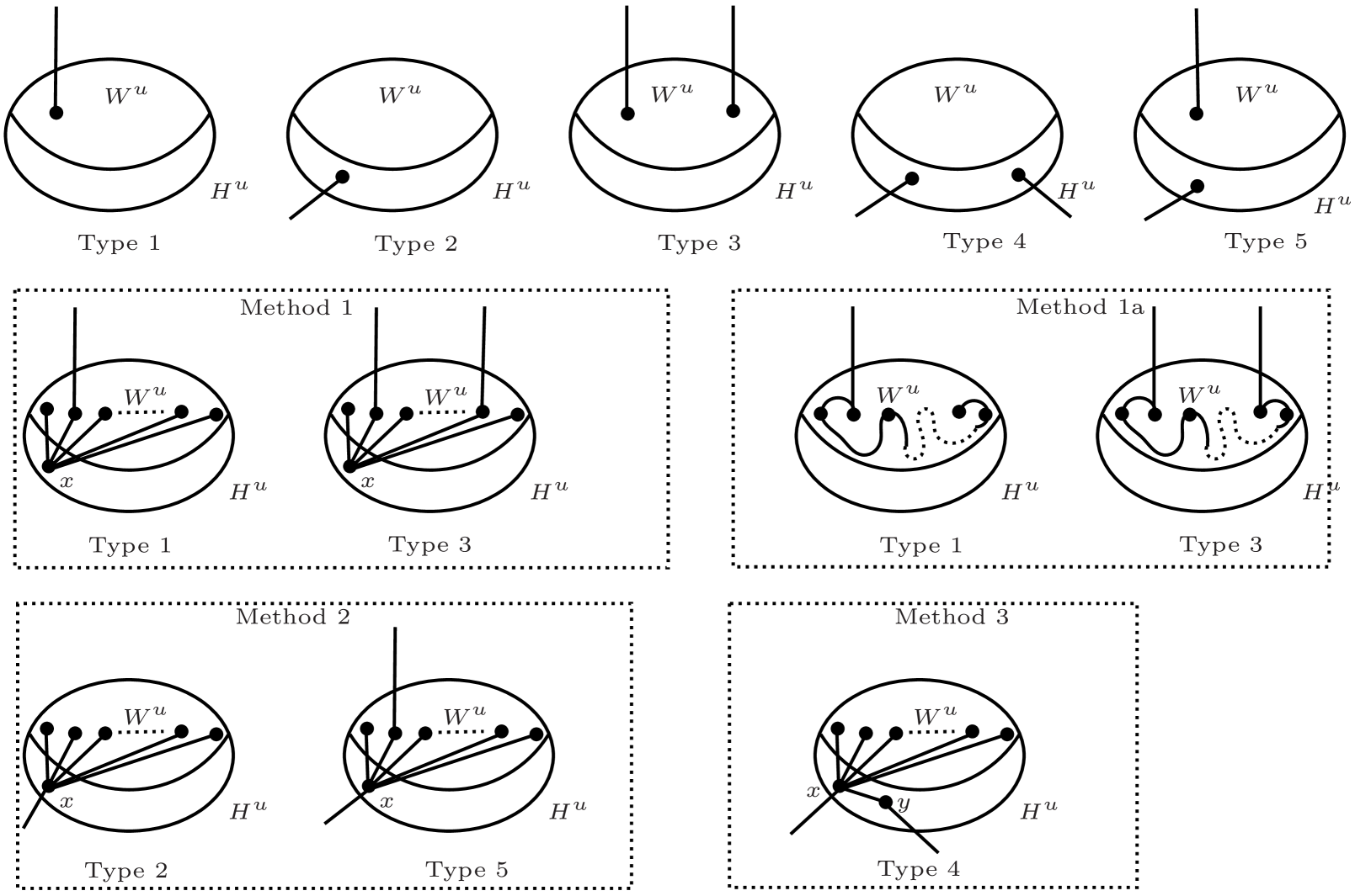
Figure 6: Five types and methods 1, 1a, 2 and 3.
We have the following five methods to choose $F_{1}^{u},\ldots,F_{c}^{u}$ for the labelled vertex $u\in G_{s+1}$ (see Figure 6).
Method 1 If $F_{i}$ is a graph of Type 1 and $|W^{u}|\geq 2$ , or $F_{i}$ is a graph of Type 3, then let $F^{u}_{i}=x\vee W^{u}$ , where $x\in R(u)$ .
Method 1a If $F_{i}$ is a graph of Type 1 and $|W^{u}|\geq 2$ , then let $F^{u}_{i}$ be a Hamiltonian path of $H^{u}[W^{u}]$ such that the vertex in $V_{u,i}$ is an endpoint of this Hamiltonian path; if $F_{i}$ is a graph of Type 3, then let $F^{u}_{i}$ be a Hamiltonian path of $H^{u}[W^{u}]$ such that the endpoints of $F_{i}$ are two vertices in $V_{u,i}$ .
Method 2 If $F_{i}$ is a graph of Type 2 or Type 5, say $x$ is the only vertex of $V_{u,i}$ with $x\notin W^{u}$ , then let $F^{u}_{i}=x\vee W^{u}$ .
Method 3 If $F_{i}$ is a graph of Type 4, say $V_{u,i}=\{x,y\}$ , then let $F^{u}_{i}=xy\cup(x\vee W^{u})$ .
Method 4 If $F_{i}$ is a graph of Type 1 and $|W^{u}|=1$ , then let $F_{i}^{u}$ be the empty graph.
It is worth noting that the method is deterministic if $F_{i}^{u}$ is a graph of Types 2, 4 and 5, or $F_{i}^{u}$ is a graph of Type 1 and $|W^{u}|=1$ . So we firstly construct these $F_{i}^{u}$ s by using Methods 2, 3 and 4, respectively, and then construct $F^{u}_{i}$ s of Type 1 with $|W^{u}|\geq 2$ and construct $F^{u}_{i}$ s of Type 3 by using Method 1 or Method 1a.
The following is an algorithm constructing $c$ internally disjoint $U$ -Steiner trees of $G$ .
Input: $U$ , $c$ and $G=S(n,\ell)$ with $|W^{root}|\geq 2$
Output: $c$ internally disjoint $U$ -Steiner trees $T^{\prime}_{1},T^{\prime}_{2},\ldots,T^{\prime}_{c}$ of $G$
1 $T^{\prime}_{1},T^{\prime}_{2},\ldots,T^{\prime}_{c}$ are empty graphs;
2 $s=n$ //(* in initial step, $G^{n}$ is a single vertex*);
3 for $s\geq 1$ do
4 for each vertex $u$ of $G_{s}$ do
5 if $u$ is an unlabelled vertex then
6 for $1\leq i\leq c$ do
7 if $u$ is a vertex of $F_{i}$ then
8 $F_{i}^{u}$ is a spanning tree of $H^{u}$ ;
9 else
10 $\ F_{i}^{u}$ is is the empty graph;
11 end if
12 $T^{\prime}_{i}=T^{\prime}_{i}\cup F_{i}^{u}$ ;
13 $i=i+1$ ;
14
15 end for
16
17 end if
18
19 if $u$ is a labelled vertex then
20 $\mu=|R(u)|$ ;
21 for $1\leq i\leq c$ do
22
23 if $T^{\prime}_{i}$ is of Type 2 or Type 5 then
24 construct $F_{i}^{u}$ by using Method 2;
25
26 end if
27
28 if $T^{\prime}_{i}$ is of Type 4 then
29 construct $F_{i}^{u}$ by using Method 3;
30
31 end if
32
33 if $T^{\prime}_{i}$ is of Type 1 and $|W^{u}|=1$ then
34 construct $F_{i}^{u}$ by using Method 4;
35
36 end if
37
38 if either $T^{\prime}_{i}$ is of Type 1 and $|W^{u}|\geq 2$ , or $T^{\prime}_{i}$ is of Type 3 then
39 if $\mu>0$ then
40 construct $F_{i}^{u}$ by using Method 1;
41 $\mu=\mu-1$ ;
42
43 end if
44
45 if $\mu\leq 0$ then
46 construct $F_{i}^{u}$ by using Method 1a;
47
48 end if
49
50 end if
51
52 $T^{\prime}_{i}=T^{\prime}_{i}\cup F_{i}^{u}$ ;
53 $i=i+1$ ;
54
55 end for
56
57 end if
58
59 end for
60 $s=s-1$ ;
61
62 end for
Algorithm 1 The construction of $c$ internally disjoint $U$ -Steiner trees of $G$
Algorithm 1 is an algorithm for finding $c$ internally disjoint $U$ -Steiner trees of $G$ . For each step of $s$ , the algorithm will construct $c$ internally disjoint $U^{s-1}$ -steiner trees $T^{\prime}_{1},T^{\prime}_{2},\ldots,T^{\prime}_{c}$ . For convenience, we denote each $T_{i}^{\prime}$ by $T_{i}^{s}$ after the $s$ step of outer “for”, that is, $T_{1}^{s},T_{2}^{s},\ldots,T_{c}^{s}$ are $c$ internally disjoint $U^{s}$ -Steiner trees in $G^{s}$ generated in Algorithm 1. If Algorithm 1 is correct, then Lines 16–40 indicate that $d_{T^{\prime}_{i}}(x)\leq 2$ for any $x\in W^{u}$ , and hence ( $\star$ ) always holds.
We now check the correctness of the algorithm. Since $F_{i}^{u}$ is deterministic when $u$ is an unlabelled vertex (Lines 5–15 of Algorithm 1), and $F_{i}^{u}$ is deterministic if $u$ is a labelled vertex and either $F_{i}^{u}$ is a graph of Types 2, 4 and 5, or $F_{i}^{u}$ is a graph of Type 1 and $|W^{u}|=1$ (Lines 19–27 of Algorithm 1), we only need to talk about the labelled vertex $u$ with $|W^{u}|\geq 2$ and check the correctness of Lines 28–36 of Algorithm 1. That is, to ensure that there exist $n_{1}(u)$ $F_{i}^{u}$ s of Type 1 and $n_{3}(u)$ $F_{i}^{u}$ s of Type 3. If $F_{i}^{u}$ is constructed by Method 1, then $F_{i}^{u}$ is a star with center in $R(u)$ (say the center of the star is $a_{i}$ ); if $F_{i}^{u}$ is constructed by Method 1a, then $F_{i}^{u}$ is a Hamiltonian path of $H^{u}$ with endpoints in $V_{u,i}$ . Since $a_{i}$ s are pairwise differently and are contained in $R(u)$ , and $H^{u}$ has at most $\lfloor|W^{u}|/2\rfloor$ Hamiltonian paths to afford by Corollary 1.4, we only need to ensure that $|R(u)|+\lfloor|W^{u}|/2\rfloor\geq n_{1}(u)+n_{3}(u)$ . Thus, we only need to prove the following result.
**Lemma 2.1**
*For each labelled vertex $u\in V(G_{s})$ with $|W^{u}|\geq 2$ , Ineq.
$$
\displaystyle n_{1}(u)+n_{3}(u)-|R(u)|\leq\lfloor|W^{u}|/2\rfloor \tag{4}
$$
holds.*
* Proof*
By Eqs. (2) and (3),
| | $\displaystyle n_{1}(u)+n_{3}(u)-|R(u)|$ | $\displaystyle=n_{1}(u)+n_{3}(u)-[\ell-|W^{u}|-n_{2}(u)-2n_{4}(u)-n_{5}(u)]$ | |
| --- | --- | --- | --- |
Since $c=\ell-\lceil k/2\rceil$ , it follows that
$$
\displaystyle n_{1}(u)+n_{3}(u)-|R(u)|=n_{4}(u)+|W^{u}|-\lceil k/2\rceil. \tag{5}
$$ Before the proof of Lemma 2.1, we give a series of claims as preliminaries.
**Claim 2**
*Suppose that $a\in V(v_{root}\overrightarrow{T}u)$ is a labelled vertex with $a\in U^{\iota}$ , where $1\leq\iota\leq n$ . If $|W^{a}|=1$ (say $W^{a}=\{x\}$ ), then $n_{5}(a)\leq 1$ . Moreover,
1. if $n_{5}(a)=1$ , then $n_{4}(x)\leq 1$ ;
1. if $n_{5}(a)=0$ , then $n_{3}(x)=n_{4}(x)=n_{5}(x)=0$ .*
* Proof*
Note that $x\in U^{\iota-1}$ . in Algorithm 1 (Lines 18–39), if $T_{i}^{\iota}$ is not a tree of Type 5 on $a$ , then $F_{i}^{a}$ is chosen such that $d_{T_{i}^{\iota-1}}(x)=1$ (here $W^{a}=\{x\}$ ); if $T^{\iota}_{i}$ is a tree of Type 5 on $a$ , then $F_{i}^{a}$ is chosen such that $d_{T_{i}^{\iota-1}}(x)=2$ . Since $|W^{a}|=1$ , there is at most one $T^{\iota}_{i}$ of Type 5 on $a$ , and hence $n_{5}(a)\leq 1$ . Furthermore, if $n_{5}(a)=1$ , then there is exact one $T_{i}^{\iota-1}$ in $G^{\ell-1}$ such that $d_{T_{i}^{\iota-1}}(x)=2$ . Hence, $n_{4}(x)\leq 1$ . If $n_{5}(a)=0$ , then $d_{T_{i}^{\iota-1}}(x)=1$ for each $T_{i}^{\iota-1}$ . Therefore, $n_{3}(x)=n_{4}(x)=n_{5}(x)=0$ . ∎
**Claim 3**
*Suppose that $a,b$ are two labelled vertices of $v_{root}\overrightarrow{T}u$ and $a\in W^{b}$ , where $a\in U^{\iota}$ for some $\iota\in[n]$ . Then there are at most $\max\{1,n_{1}(b)+n_{3}(b)-|R(b)|+1\}$ $T_{i}^{\iota}$ s such that $d_{T_{i}^{\iota}}(a)=2$ . Furthermore, $n_{4}(a)\leq\max\{1,n_{1}(b)+n_{3}(b)-|R(b)|+1\}$ .*
* Proof*
Since $a\in W^{b}$ and $a\in U^{\iota}$ , it follows that $b\in U^{\iota+1}$ . For an $i\in[c]$ with $d_{T_{i}^{\iota}}(a)=2$ , we have that either $F_{i}^{b}$ is a Hamiltonian path of the clique $H^{b}[W^{b}]$ , or $a\in V_{b,i}\cap W^{b}$ for some $i\in[c]$ (recall that $V_{b,i}=\{z\in V(H^{b}):z\mbox{ is an end vertex of some edge in }E_{b,i}\}$ , where $E_{b,i}$ is the set of edges in $T_{i}^{\iota+1}$ incident with $b$ ). Hence, if there are $h$ edge-disjoint $F_{i}^{b}$ s that are constructed as Hamiltonian paths of $H^{b}[W^{b}]$ , then there are at most $h+1$ internally disjoint $U^{\iota}$ -Steiner trees $T_{i}^{\iota}$ such that $d_{T_{i}^{\iota}}(a)=2$ . By the definition of $n_{4}(a)$ , we have that $n_{4}(a)\leq h+1$ . In Algorithm 1 (Lines 28–36), if $n_{1}(b)+n_{3}(b)-|R(b)|>0$ , then there are at most $n_{1}(b)+n_{3}(b)-|R(b)|$ $F_{i}^{b}$ s that are constructed as Hamiltonian paths in $H^{b}[W^{b}]$ ; if $n_{1}(b)+n_{3}(b)-|R(b)|\leq 0$ , there is no $F_{i}^{b}$ that is constructed as a Hamiltonian path in $H^{b}[W^{b}]$ . Hence, $h\leq\max\{0,n_{1}(b)+n_{3}(b)-|R(b)|\}$ . Thus, there are at most $\max\{1,n_{1}(b)+n_{3}(b)-|R(b)|+1\}$ internally disjoint $U^{\iota}$ -Steiner trees $T_{i}^{\iota}$ such that $d_{T_{i}^{\iota}}(a)=2$ , and $n_{4}(a)\leq\max\{1,n_{1}(b)+n_{3}(b)-|R(b)|+1\}$ . ∎
**Claim 4**
*Let $a\in V(v_{root}\overrightarrow{T}u)$ be a labelled vertex, where $a\in U^{\iota}$ for some $\iota\in[n]$ . If $n_{4}(a)\leq 1$ and $2\leq|W^{a}|\leq\left\lceil k/2\right\rceil-1$ , then $n_{1}(a)+n_{3}(a)-|R(a)|\leq 0$ . Moreover, for each vertex $x\in W^{a}$ , there is at most one $T_{i}^{\iota-1}$ such that $d_{T_{i}^{\iota-1}}(x)=2$ .*
* Proof*
Since $n_{4}(a)\leq 1$ and $|W^{a}|\leq\left\lceil k/2\right\rceil-1$ , it follows from Eq. (5) that $n_{1}(a)+n_{3}(a)-|R(a)|=|W^{a}|-\left\lceil k/2\right\rceil+1\leq 0.$ By Claim 3, for each vertex $x\in W^{a}$ , there is at most one $T_{i}^{a}$ such that $d_{T_{i}^{\iota-1}}(x)\leq 2$ . ∎
**Claim 5**
*Let $a\in V(v_{root}\overrightarrow{T}u)$ be a labelled vertex, where $a\in U^{\iota}$ for some $\iota\in[n]$ . If $n_{4}(a)\leq 1$ and $\left\lceil k/2\right\rceil\leq|W^{a}|\leq k-1$ , then $n_{1}(a)+n_{3}(a)-|R(a)|\leq\lfloor|W^{a}|/2\rfloor$ . Moreover, for each $x\in W^{a}$ ,
1. if $n_{4}(a)=1$ , then there are at most $|W^{a}|-\left\lceil k/2\right\rceil+2$ internally disjoint $U^{\iota-1}$ -Steiner trees $T_{i}^{\iota-1}$ such that $d_{T_{i}^{\iota-1}}(x)=2$ ;
1. if $n_{4}(a)=0$ , then there are at most $|W^{a}|-\left\lceil k/2\right\rceil+1$ internally disjoint $U^{\iota-1}$ -Steiner trees $T_{i}^{\iota-1}$ such that $d_{T_{i}^{\iota-1}}(x)=2$ .*
* Proof*
Since $n_{4}(a)\leq 1$ , it follows from Eq. (5) that
| | $\displaystyle n_{1}(a)+n_{3}(a)-|R(a)|$ | $\displaystyle\leq|W^{a}|-\left\lceil k/2\right\rceil+n_{4}(a)$ | |
| --- | --- | --- | --- |
and the equality indicates $n_{4}(a)=1$ . If $|W^{a}|\leq k-2$ , then
$$
n_{1}(a)+n_{3}(a)-|R(a)|\leq|W^{a}|-\left\lceil(|W^{a}|+2)/2\right\rceil+1\leq
\left\lfloor|W^{a}|/2\right\rfloor;
$$
if $|W^{a}|=k-1$ and $k$ is even, then
$$
n_{1}(a)+n_{3}(a)-|R(a)|=|W^{a}|-\left\lceil(|W^{a}|+1)/2\right\rceil+1=\left
\lfloor(|W^{a}|+1)/2\right\rfloor=\left\lfloor|W^{a}|/2\right\rfloor;
$$
if $|W^{a}|=k-1$ and $k$ is odd, then
$$
n_{1}(a)+n_{3}(a)-|R(a)|=(k-1)-\left\lceil k/2\right\rceil+1\leq\left\lfloor k
/2\right\rfloor=\left\lfloor(k-1)/2\right\rfloor=\left\lfloor|W^{a}|/2\right\rfloor.
$$
Therefore, $n_{1}(a)+n_{3}(a)-|R(a)|\leq\left\lfloor|W^{a}|/2\right\rfloor$ . By Eq. (5) and Claim 3, if $n_{4}(a)=1$ , then for each vertex $x\in W^{a}$ , there are at most $n_{1}(a)+n_{3}(a)-|R(a)|+1=|W^{a}|-\left\lceil k/2\right\rceil+2$ internally disjoint $U^{\iota-1}$ -Steiner trees $T_{i}^{\iota-1}$ such that $d_{T_{i}^{\iota-1}}(x)=2$ ; if $n_{4}(a)=0$ , then for each vertex $x\in W^{a}$ , there are at most $n_{1}(a)+n_{3}(a)-|R(a)|+1=|W^{u}|-\left\lceil k/2\right\rceil+1$ internally disjoint $U^{\iota-1}$ -Steiner trees $T_{i}^{\iota-1}$ such that $d_{T_{i}^{\iota-1}}(x)=2$ . ∎
**Claim 6**
*Suppose $a,b\in V(\overrightarrow{T})$ , $a\prec b$ and $a\overrightarrow{T}b=az_{1}z_{2}\ldots z_{p}b$ , where $a\in U^{\iota}$ for some $\iota\in[n]$ . If $|W^{z_{i}}|\leq\lceil k/2\rceil-1$ for each $i\in[p]$ , and either $|W^{a}|=1$ or $2\leq|W^{a}|\leq\lceil k/2\rceil-1$ and $n_{4}(a)\leq 1$ , then $n_{4}(b)\leq 1$ .*
* Proof*
Since $a\in U^{\iota}$ , it follows that $z_{q}\in U^{\iota-q}$ for each $q\in[p]$ and $b\in U^{\iota-p-1}$ . Since $|W^{a}|=1$ or $2\leq|W^{a}|\leq\lceil k/2\rceil-1$ and $n_{4}(a)\leq 1$ , by Claims 2 and 4, there are at most one $T_{i}^{\iota-1}$ such that $d_{T_{i}^{\iota-1}}(z_{1})=2$ . Hence, $n_{4}(z_{1})\leq 1$ . Since $|W^{z_{1}}|\leq\lceil k/2\rceil-1$ and $n_{4}(z_{1})\leq 1$ , by Claims 2 and 4, there are at most one $T_{i}^{\iota-2}$ such that $d_{T_{i}^{\iota-2}}(z_{2})=2$ . Hence, $n_{4}(z_{2})\leq 1$ . Repeat this progress, we can get that $n_{4}(z_{p})\leq 1$ . Since $|W^{z_{p}}|\leq\lceil k/2\rceil-1$ and $n_{4}(z_{p})\leq 1$ , by Claims 2 and 4, there are at most one $T_{i}^{\iota-p-1}$ such that $d_{T_{i}^{\iota-p-1}}(b)=2$ . Hence, $n_{4}(b)\leq 1$ . ∎
**Claim 7**
*Suppose $|W^{v_{root}}|\leq\lceil k/2\rceil$ , $b\in V(\overrightarrow{T})$ and $v_{root}\overrightarrow{T}b=v_{root}z_{1}z_{2}\ldots z_{p}b$ . If $|W^{z_{i}}|=1$ for each $i\in[p]$ , then $n_{4}(b)=0$ .*
* Proof*
Since $|W^{v_{root}}|\leq\lceil k/2\rceil$ , by Claim 1, $d_{T_{i}^{n-1}}(z_{1})=1$ for each $U^{n-1}$ -Steiner tree $T_{i}^{n-1}$ . Hence, $n_{3}(z_{1})=n_{4}(z_{1})=n_{5}(z_{1})=0$ . Since $|W^{z_{1}}|=1$ and $n_{5}(z_{1})=0$ , by the second statement of Claim 2, $n_{3}(z_{2})=n_{4}(z_{2})=n_{5}(z_{2})=0$ . Since $|W^{z_{2}}|=1$ and $n_{5}(z_{2})=0$ , by the second statement of Claim 2, $n_{3}(z_{3})=n_{4}(z_{3})=n_{5}(z_{3})=0$ . Repeat this process, we get that $n_{4}(b)=0$ . ∎
**Claim 8**
*Suppose that $a,b$ are two labelled vertices and $a\in W^{b}$ , where $a\in U^{\iota}$ for some $\iota\in[n]$ . If $k$ is even and $|W^{b}|=|W^{a}|=k/2$ , then $n_{1}(a)+n_{3}(a)-|R(a)|\leq\lfloor|W^{a}|/2\rfloor$ and the following hold.
1. If $b=v_{root}$ , then for each vertex $x\in W^{a}$ , there is at most one $T_{i}^{\iota-1}$ such that $d_{T_{i}^{\iota-1}}(x)=2$ .
1. If $b\neq v_{root}$ , then for each vertex $x\in W^{a}$ , there are at most two $T_{i}^{\iota-1}$ s such that $d_{T_{i}^{\iota-1}}(x)=2$ .*
* Proof*
Suppose $b=v_{root}$ . Then by Claim 1, $n_{4}(a)=0$ . Thus,
$$
n_{1}(a)+n_{3}(a)-|R(a)|=n_{4}(a)+|W^{a}|-k/2=|W^{a}|-k/2=0.
$$
By Claim 3, for each vertex $x\in W^{a}$ , there is at most one $T_{i}^{\iota-1}$ such that $d_{T_{i}^{\iota-1}}(x)=2$ . Now assume that $b\neq v_{root}$ . Without loss of generality, suppose $v_{root}\overrightarrow{T}b=v_{root}v_{1}v_{2}\ldots v_{p}b$ . By Fact 1, we have that $|W^{root}|=2\leq k/2$ and $|W^{v_{i}}|=1$ for each $i\in[p]$ . By Claim 7, $n_{4}(b)=0$ . By Claim 3,
| | $\displaystyle n_{4}(a)$ | $\displaystyle\leq\max\{1,n_{1}(b)+n_{3}(b)-|R(b)|+1\}$ | |
| --- | --- | --- | --- |
By Claim 3 again, for each vertex $x\in W^{a}$ , there are at most two $T_{i}^{\iota-1}$ such that $d_{T_{i}^{\iota-1}}(x)=2$ . ∎
With the above preparations, we now prove Lemma 2.1. Recall that $u\in V(G_{s})$ is a labelled vertex with $|W^{u}|\geq 2$ . Then each vertex of $V(v_{root}\overrightarrow{T}u)$ is also a labelled vertex. Suppose that $v^{*}$ is the maximum vertex of $v_{root}\overrightarrow{T}u$ such that one of the following holds (if such vertex $v^{*}$ exists).
1. $|W^{v^{*}}|=1$ ,
1. $2\leq|W^{v^{*}}|\leq\lceil k/2\rceil-1$ and $n_{4}(v^{*})\leq 1$ .
We distinguish the following two cases to show this lemma, that is, to prove Ineq. (4) holds (recall that the Ineq. (4) is $n_{1}(u)+n_{3}(u)-|R(u)|\leq\lfloor|W^{u}|/2\rfloor$ ).
**Case 1**
*$v^{*}$ exists.*
Let $\overrightarrow{P}=v^{*}\overrightarrow{T}u=v^{*}z_{1}z_{2}\ldots z_{p}u$ . By the maximality of $v^{*}$ , we have that $|W^{z_{i}}|\geq 2$ for each $i\in[p]$ . If $|\overrightarrow{P}|=1$ , then $v^{*}=u$ . Since $|W^{u}|\geq 2$ , it follows from ( $ii$ ) that $2\leq|W^{u}|\leq\lceil k/2\rceil-1$ and $n_{4}(u)\leq 1$ . By Claim 4, we have that $n_{1}(u)+n_{3}(u)-|R(u)|\leq 0$ , and Ineq. (4) holds. Thus, we assume that $|\overrightarrow{P}|\geq 2$ below. By Claim 6, we have that
$$
\displaystyle n_{4}(z_{1})\leq 1. \tag{6}
$$
Thus, by the maximality of $v^{*}$ , we have that $|W^{z_{1}}|\geq\lceil k/2\rceil$ . Since $|W^{v_{root}}|+|W^{z_{1}}|\leq k+1$ (by Fact 1) and $|W^{v_{root}}|\geq 2$ , it follows that $|W^{z_{1}}|\leq k-1$ . Hence,
$$
\displaystyle\lceil k/2\rceil\leq|W^{z_{1}}|\leq k-1. \tag{7}
$$
**Subcase 1.1**
*$p=0$ .*
Then $\overrightarrow{P}=v^{*}\overrightarrow{T}u=v^{*}u$ and $z_{1}=u$ . Since $n_{4}(u)\leq 1$ and $\lceil k/2\rceil\leq|W^{u}|\leq k-1$ by Ineqs. (6) and (7), it follows from Claim 5 that $n_{1}(u)+n_{3}(u)-|R(u)|\leq\lfloor|W^{u}|/2\rfloor$ , Ineq. (4) holds.
**Subcase 1.2**
*$p=1$ .*
Then $\overrightarrow{P}=v^{*}\overrightarrow{T}u=v^{*}z_{1}u$ and $u=z_{2}$ . By Fact 1, we have that
$$
\displaystyle|W^{z_{1}}|+|W^{u}|+|W^{v_{root}}|-2\leq k. \tag{8}
$$
Hence $|W^{z_{1}}|+|W^{u}|\leq k$ . Recall that $|W^{z_{1}}|\geq\lceil k/2\rceil$ . If $|W^{u}|\geq\lceil k/2\rceil$ , then $k$ is even and $|W^{z_{1}}|=|W^{u}|=k/2$ . By Claim 8, we have that $n_{1}(u)+n_{3}(u)-|R(u)|\leq\lfloor|W^{u}|/2\rfloor$ . Therefore, Ineq. (4) holds. Now, we assume that $2\leq|W^{u}|\leq\lceil k/2\rceil-1$ . Since $n_{4}(z_{1})\leq 1$ and $k-1\geq|W^{z_{1}}|\geq\lceil k/2\rceil$ , by Claim 5, there are at most $|W^{z_{1}}|-\left\lceil k/2\right\rceil+2$ internally disjoint $U^{s}$ -Steiner trees $T_{i}^{s}$ such that $d_{T_{i}^{s}}(u)=2$ (note that $u\in G_{s}$ ). Hence, $n_{4}(u)\leq|W^{z_{1}}|-\left\lceil k/2\right\rceil+2$ . Thus, by Eq. (5),
$$
n_{1}(u)+n_{3}(u)-|R(u)|=n_{4}(u)+|W^{u}|-\left\lceil k/2\right\rceil\leq|W^{u
}|+|W^{z_{1}}|-2\left\lceil k/2\right\rceil+2.
$$
If $|W^{u}|+|W^{z_{1}}|\leq k-1$ or $k$ is odd, then $n_{1}(u)+n_{3}(u)-|R(u)|\leq 1\leq\lfloor|W^{u}|/2\rfloor$ , Ineq. (4) holds. Thus, assume that $|W^{u}|+|W^{z_{1}}|=k$ (recall that $|W^{u}|+|W^{z_{1}}|\leq k$ ) and $k$ is even below ( $k\geq 4$ ). Since $|W^{z_{1}}|\geq\lceil k/2\rceil$ , it follows that $|W^{u}|\leq k/2$ . Suppose that $v_{root}\overrightarrow{T}z_{p}=v_{root}w_{1}w_{2}\ldots w_{q}v^{*}z_{p}$ . Since $|W^{v_{root}}|\geq 2$ , it follows from Ineq. (8) and Fact 1 that $|W^{v_{root}}|=2\leq k/2$ and $|W^{w_{1}}|=\ldots=|W^{w_{q}}|=|W^{v^{*}}|=1$ . According to Claim 7, we have that $n_{4}(u)=0$ . Hence,
| | $\displaystyle n_{1}(u)+n_{3}(u)-|R(u)|$ | $\displaystyle=n_{4}(u)+|W^{u}|-\left\lceil k/2\right\rceil\leq 0\leq\lfloor|W^ {u}|/2\rfloor,$ | |
| --- | --- | --- | --- |
the Ineq. (4) holds.
**Subcase 1.3**
*$p\geq 2$ .*
Then $u\succeq z_{3}$ . Recall that $|W^{z_{i}}|\geq 2$ for each $i\in[p]$ . Since
$$
\displaystyle|W^{v_{root}}|+|W^{z_{1}}|+|W^{z_{2}}|+|W^{z_{3}}|-3\leq k \tag{9}
$$
and $|W^{z_{1}}|\geq\lceil k/2\rceil$ , it follows that $|W^{z_{2}}|,|W^{z_{3}}|\leq\lfloor k/2\rfloor-1$ and $|W^{z_{1}}|+|W^{z_{2}}|\leq k-1$ . On the other hand, since $|W^{z_{3}}|\geq 2$ , it follows that $k\geq 6$ . Without loss of generality, suppose $z_{2}\in U^{\iota}$ . Recall Ineqs. (6) and (7), and combine with Claim 5, there are at most $|W^{z_{1}}|-\left\lceil\frac{k}{2}\right\rceil+2$ internally disjoint $U^{\iota}$ -Steiner trees $T_{i}^{\iota}$ such that $d_{T_{i}^{\iota}}(z_{2})=2$ . Hence, $n_{4}(z_{2})\leq|W^{z_{1}}|-\left\lceil\frac{k}{2}\right\rceil+2$ . By Claim 3, $n_{4}(z_{3})\leq\max\{1,n_{4}(z_{2})+|W^{z_{2}}|-\lceil k/2\rceil+1\}$ . However, by the maximality of $v^{*}$ , we have that $n_{4}(z_{3})\geq 2$ . Hence,
$$
\displaystyle n_{4}(z_{3})\leq n_{4}(z_{2})+|W^{z_{2}}|-\lceil k/2\rceil+1\leq
|W^{z_{1}}|+|W^{z_{2}}|-2\lceil k/2\rceil+3. \tag{10}
$$
Since $|W^{z_{1}}|+|W^{z_{2}}|\leq k-1$ , it follows that if $k$ is odd or $|W^{z_{1}}|+|W^{z_{2}}|\leq k-2$ , then $n_{4}(z_{3})\leq 1$ , a contradiction. Hence, $k$ is even and $|W^{z_{1}}|+|W^{z_{2}}|=k-1$ . This implies that $|W^{z_{3}}|=n_{4}(z_{3})=2$ by Ineqs. (9) and (10). Since $k\geq 6$ , it follows that $n_{4}(z_{3})+|W^{z_{3}}|-\lceil k/2\rceil\leq 1\leq\lfloor|W^{z_{3}}|/2\rfloor$ . Recall that $u\succeq z_{3}$ . If $v_{3}=u$ , then
$$
n_{1}(u)+n_{3}(u)-|R(u)|=n_{4}(u)+|W^{u}|-\lceil k/2\rceil\leq\lfloor|W^{u}|/2\rfloor,
$$
Ineq. (4) holds. If $u\succ z_{3}$ , then since
| | $\displaystyle|W^{v_{root}}|+|W^{z_{1}}|+|W^{z_{2}}|+|W^{z_{3}}|+|W^{u}|-4\leq k,$ | |
| --- | --- | --- |
we have that
| | $\displaystyle|W^{u}|\leq k+4-(|W^{v_{root}}|+|W^{z_{1}}|+|W^{z_{2}}|+|W^{z_{3} }|)=1,$ | |
| --- | --- | --- |
a contradiction.
**Case 2**
*$v^{*}$ does not exist.*
Let $\overrightarrow{P}=v_{root}\overrightarrow{T}u=v_{root}z_{1}\ldots,z_{t}u$ . Since $v^{*}$ does not exist, for each vertex $z\in V(\overrightarrow{P})$ , either $2\leq|W^{z}|\leq\lceil k/2\rceil-1$ and $n_{4}(z)\geq 2$ , or $|W^{z}|\geq\lceil k/2\rceil$ . Since $n_{4}(v_{root})=0$ , it follows that $|W^{v_{root}}|\geq\lceil k/2\rceil$ . By Claim 1, $n_{4}(z_{1})\leq|W^{v_{root}}|-\lceil k/2\rceil$ .
**Subcase 2.1**
*$|W^{z_{1}}|\geq\lceil k/2\rceil$ .*
Since $|W^{v_{root}}|,|W^{z_{1}}|\geq\lceil k/2\rceil$ , we have that $t\leq 1$ . Otherwise,
$$
\sum_{z\in V(\overrightarrow{P})}|W^{z}|-(|\overrightarrow{P}|-1)>k,
$$
which contradicts Fact 1. Moreover, if $t=1$ , then $k$ is even, $|W^{v_{root}}|=|W^{z_{1}}|=k/2$ and $|W^{u}|=2$ . Suppose that $t=0$ . Then $u=z_{1}$ , and hence $n_{4}(u)\leq|W^{v_{root}}|-\lceil k/2\rceil$ . Thus
| | $\displaystyle n_{1}(u)+n_{3}(u)-|R(u)|$ | $\displaystyle=n_{4}(u)+|W^{u}|-\lceil k/2\rceil$ | |
| --- | --- | --- | --- |
Ineq. (4) holds. Suppose $t=1$ . Then $\overrightarrow{P}=v_{root}z_{1}u$ . Hence, $k$ is even ( $k\geq 4$ ), $|W^{v_{root}}|=|W^{z_{1}}|=k/2$ and $|W^{u}|=2$ . By the first statement of Claim 8 (here, we regard $v_{root}$ and $z_{1}$ as the vertices $b$ and $a$ in Claim 8, respectively, and then $u$ can be regarded as the vertex $x$ in Claim 8), we have that $n_{4}(u)\leq 1$ . Hence,
$$
n_{1}(u)+n_{3}(u)-|R(u)|=n_{4}(u)+|W^{u}|-\lceil k/2\rceil\leq 1\leq\lfloor|W^
{u}|/2\rfloor,
$$
Ineq. (4) holds.
**Subcase 2.2**
*$2\leq|W^{z_{1}}|\leq\lceil k/2\rceil-1$ .*
Recall that $n_{4}(z_{1})=|W^{v_{root}}|-\lceil k/2\rceil$ . Since $n_{4}(z_{1})\geq 2$ , $|W^{v_{root}}|\geq\lceil k/2\rceil+2$ . If $|W^{v_{root}}|+|W^{z_{1}}|=k+1$ , then $v=v_{root}$ , $u=z_{1}$ and
$$
n_{1}(u)+n_{3}(u)-|R(u)|=n_{4}(u)+|W^{u}|-\lceil k/2\rceil\leq 1\leq\lfloor|W^
{u}|/2\rfloor.
$$
Thus, suppose $|W^{v_{root}}|+|W^{z_{1}}|\leq k$ . Then
$$
n_{1}(z_{1})+n_{3}(z_{1})-|R(z_{1})|=n_{4}(z_{1})+|W^{z_{1}}|-\lceil k/2\rceil
\leq 0.
$$
If $z_{1}=u$ , then $n_{1}(u)+n_{3}(u)-|R(u)|\leq 0,$ Ineq. (4) holds. Now, assume that $z_{1}\neq u$ . Then $z_{2}$ exists. By Claim 3, $n_{4}(z_{2})\leq 1$ . Since $z_{2}$ is not a candidate of $v^{*}$ , it follows that $|W^{z_{2}}|\geq\lceil k/2\rceil$ . Since $|W^{v_{root}}|\geq\lceil k/2\rceil+2,|W^{z_{2}}|\geq\lceil k/2\rceil$ and $|W^{z_{1}}|\geq 2$ , it follows that $|W^{v_{root}}|+|W^{z_{1}}|+|W^{z_{2}}|-2\geq k+2$ , which contradicts Fact 1. ∎
With the conclusion of Lemma 2.1, the proof of Theorem 2.1 is completed.
### 2.3 Proof of Theorem 1.5
We first consider $3\leq k\leq\ell$ . The lower bound $\ell-\lceil k/2\rceil\leq\kappa_{k}(S(n,\ell))\leq\lambda_{k}(S(n,\ell))$ can be obtained from Theorem 2.1 directly. For the upper bounds of $\kappa_{k}(S(n,\ell))$ and $\lambda_{k}(S(n,\ell))$ , consider the graph $G_{n-1}$ . Let $V(G_{n-1})=\{u_{1},\ldots,u_{\ell}\}$ , $U=\{x_{1},\ldots,x_{k}\}$ and $x_{i}\in A_{n-1,u_{i}}$ , where $k\leq\ell$ . Suppose there are $p$ edge-disjoint $U$ -Steiner trees $T^{\prime}_{1},\ldots,T^{\prime}_{p}$ of $G=S(n,\ell)$ and $\mathcal{P}=\{A_{n-1,u}:u\in V(G_{n-1})\}$ . Let $T^{*}_{i}=T^{\prime}_{i}/\mathcal{P}$ for $i\in[p]$ . Then $T^{*}_{1},\ldots,T^{*}_{p}$ are edge-disjoint connected graphs of $G_{n-1}$ containing $\{u_{1},\ldots,u_{k}\}$ . Thus, $p\leq\lambda_{k}(G_{n-1})=\lambda_{k}(K_{\ell})=\ell-\lceil k/2\rceil$ . Therefore, $\kappa_{k}(S(n,\ell))\leq\lambda_{k}(S(n,\ell))\leq\ell-\lceil k/2\rceil$ , the upper bound follows.
Now consider the case $\ell+1\leq k\leq{\ell}^{n}$ . By Theorem 1.2, $\lambda_{k}(S(n,\ell))\geq\lfloor\ell/2\rfloor$ . Since $\lambda_{k}(S(n,\ell))\leq\lambda_{\ell}(S(n,\ell))=\lfloor\ell/2\rfloor$ , it follows that $\kappa_{k}(S(n,\ell))\leq\lambda_{k}(S(n,\ell))\leq\lfloor\ell/2\rfloor$ . Therefore, $\lambda_{k}(S(n,\ell))=\lfloor\ell/2\rfloor$ and $\kappa_{k}(S(n,\ell))\leq\lfloor\ell/2\rfloor$ . The proof is completed.
## 3 Some network properties
Generalized connectivity is a graph parameter to measure the stability of networks. In the following part, we will give the following other properties of Sierpiński graphs.
The Sierpiński graph(networks) is obtained after $t$ iteration as $S(t,\ell)$ that has $N_{t}$ nodes and $E_{t}$ edges, where $t=0,1,2,\cdots,T-1$ , and $T$ is the total number of iterations, and our generation process can be illustrated as follows.
<details>
<summary>x3.png Details</summary>
### Visual Description
\n
## Mathematical Function Plot: Comparison of Two Exponential Growth Functions
### Overview
The image is a 2D line plot generated by mathematical software (likely Mathematica or similar). It displays two exponential growth functions plotted against a common independent variable, `t`. The plot demonstrates the rapid, accelerating growth characteristic of exponential functions, with one function consistently outpacing the other.
### Components/Axes
* **X-Axis (Horizontal):**
* **Label:** Implicitly represents the variable `t` (as indicated by the function definitions in the legend).
* **Scale:** Linear scale.
* **Range:** Approximately 0 to 14.
* **Major Tick Marks & Labels:** Located at intervals of 2: `2`, `4`, `6`, `8`, `10`, `12`, `14`.
* **Y-Axis (Vertical):**
* **Label:** Implicitly represents the function value, `f(t)`.
* **Scale:** Linear scale.
* **Range:** 0 to 2.5 x 10⁶ (2,500,000).
* **Major Tick Marks & Labels:** Located at intervals of 500,000: `500 000`, `1.0 x 10⁶`, `1.5 x 10⁶`, `2.0 x 10⁶`, `2.5 x 10⁶`.
* **Legend:**
* **Position:** Centered vertically on the right side of the plot area, outside the axes.
* **Content:**
1. **Blue Line:** Labeled with the mathematical expression `3^t`.
2. **Orange Line:** Labeled with the mathematical expression `1/2 (3^(t+1) - 3)`.
* **Plot Area:** Contains two smooth, continuous curves originating near the origin (0,0) and rising sharply to the right.
### Detailed Analysis
* **Data Series 1 (Blue Line - `3^t`):**
* **Trend Verification:** The line exhibits classic exponential growth. It starts with a very shallow slope near t=0, remains close to the x-axis until approximately t=8, and then curves upward with a rapidly increasing slope.
* **Approximate Data Points (Visual Estimation):**
* At t=10: y ≈ 59,000 (5.9 x 10⁴)
* At t=12: y ≈ 531,000 (5.31 x 10⁵)
* At t=13: y ≈ 1,594,000 (1.594 x 10⁶)
* At t=14: y ≈ 4,782,000 (4.782 x 10⁶) - *Note: This point is beyond the top of the plotted y-axis range.*
* **Data Series 2 (Orange Line - `1/2 (3^(t+1) - 3)`):**
* **Trend Verification:** This line also shows exponential growth. It follows a similar shape to the blue line but is consistently positioned above it. The vertical gap between the orange and blue lines widens significantly as `t` increases.
* **Approximate Data Points (Visual Estimation):**
* At t=10: y ≈ 88,000 (8.8 x 10⁴)
* At t=12: y ≈ 796,000 (7.96 x 10⁵)
* At t=13: y ≈ 2,391,000 (2.391 x 10⁶)
* At t=14: y ≈ 7,173,000 (7.173 x 10⁶) - *Note: This point is well beyond the top of the plotted y-axis range.*
* **Relationship Between Series:** For any given `t`, the value of the orange function is greater than the blue function. The ratio between them approaches a constant. Mathematically, `1/2 (3^(t+1) - 3) = (3/2)*3^t - 3/2`. For large `t`, this is approximately `(3/2)*3^t`, meaning the orange line is roughly 1.5 times the height of the blue line. This visual relationship is confirmed in the plot.
### Key Observations
1. **Exponential Growth:** Both functions demonstrate the "hockey stick" curve of exponential growth, where the rate of increase itself increases.
2. **Divergence:** The absolute difference between the two functions grows dramatically with `t`. At t=10, the difference is ~29,000. By t=13, the difference is ~797,000.
3. **Scale:** The y-axis uses scientific notation (`x 10⁶`) to accommodate the very large numbers generated by the functions within a limited plot height.
4. **Clipping:** The plotted lines extend beyond the upper limit of the y-axis (2.5 x 10⁶) shortly after t=13, indicating the functions' values exceed the displayed range.
### Interpretation
This plot is a direct visual comparison of two related exponential functions. The function `1/2 (3^(t+1) - 3)` can be algebraically simplified to `(3/2)*3^t - 3/2`. The graph visually proves that this function is not merely a scaled version of `3^t`; it has a larger base multiplier (1.5 vs 1) and a constant offset (-1.5), which becomes negligible at high `t`.
The key takeaway is the power of exponential growth and how small differences in the function's formula (a multiplier of 1.5 versus 1) lead to enormous differences in output over time. This principle is fundamental in fields like finance (compound interest), biology (population growth), and computer science (algorithmic complexity). The plot serves as a clear, intuitive demonstration that the orange function will always dominate the blue one for positive `t`, and the gap between them will become astronomically large.
</details>
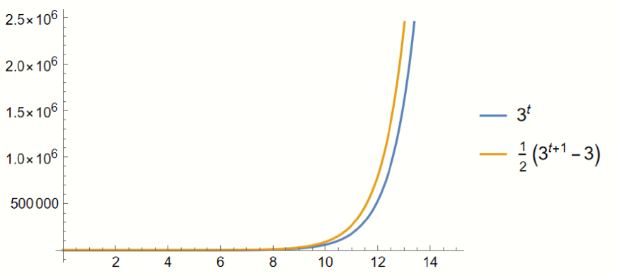
Figure 7: The Function of $E_{t}=3^{t}$ and $N_{t}=\frac{3^{t+1}-3}{2}$
Step 1: Initialization. Set $t=0$ , $G_{1}$ is a complete graph of order $\ell$ , and thus $N_{1}=\ell$ and $E_{1}=\binom{\ell}{2}$ . Set $G_{1}=S(1,\ell)$ .
Step 2: Generation of $G_{t+1}$ from $G_{t}$ . Let $S^{1}(t,\ell),S^{2}(t,\ell),\ldots,S^{\ell}(t,\ell)$ be all Sierpiński graphs added at Step $t$ , where $S^{i}(t,\ell)\cong S(t,\ell)$ ( $1\leq i\leq\ell$ ). At Step $t+1$ , we add one edge (bridge edge) between $S^{i}(t,\ell)$ and $S^{j}(t,\ell)$ , $i\neq j$ , namely the edge between vertices $\langle ij\cdots j\rangle$ and $\langle ji\cdots i\rangle$ .
For Sierpiński graphs $G_{t}=S(t,\ell)$ , its order and size are $N_{t}=\ell^{t}$ and $E_{t}=\frac{\ell^{t+1}-\ell}{2}$ , respectively; see Table 2 and Figure 7 (for $\ell=3$ ).
Table 2: The size and order of $G_{t}$ for $\ell=3$
| $t$ | 1 | 2 | 3 | 4 | 5 | 6 | t |
| --- | --- | --- | --- | --- | --- | --- | --- |
| $N_{t}$ | 3 | 9 | 27 | 81 | 242 | 729 | $\ell^{t}$ |
| $E_{t}$ | 3 | 12 | 39 | 120 | 363 | 1092 | $\frac{\ell^{t+1}-\ell}{2}$ |
The degree distribution for $t$ times are
$$
\left(\underbrace{\ell-1,\ell-1,\cdots,\ell-1}_{\ell},\underbrace{\ell,\ell,
\ell,\cdots,\ell}_{\ell^{t}-\ell}\right). \tag{11}
$$
From Equation 11, the instantaneous degree distribution is $P(\ell-1,t)=1/\ell^{t-1}$ for $t=2,\cdots,T$ and $P(\ell,t)=(\ell^{t}-\ell)/\ell^{t}$ for $t=2,\cdots,T$ . Note that the density of Sierpiński graphs is $\rho=E_{t}/\binom{N_{t}}{2}\rightarrow 0$ for $t\rightarrow+\infty$ . For large enough $\ell$ and any $1\leq k\leq\ell$ , we have $|\{v\in V(G)|d_{S(t,\ell)}(v)|\geq k\}\approx|V(S(t,\ell))|$ .
**Theorem 3.1**
*[11] If $n\in\mathbb{N}$ and $G$ is a graph, then $\kappa\left(S(n,G)\right)=\kappa(G)$ and $\lambda\left(S(n,G)\right)=\lambda(G)$ .*
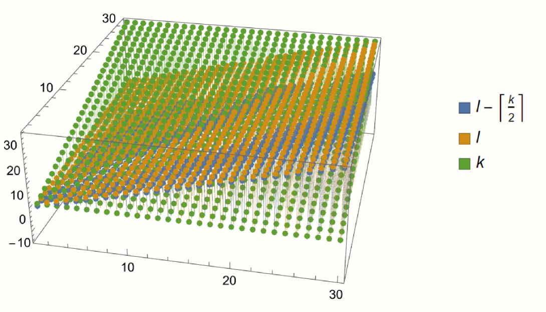
From Theorem 3.1, we have $\kappa\left(S(n,\ell)\right)=\kappa(K_{\ell})=\ell-1$ and $\lambda\left(S(n,\ell)\right)=\lambda(K_{\ell})=\ell-1$ . Note that $\lambda_{k}(S(n,\ell))=\ell-\left\lceil k/2\right\rceil$ and $\kappa_{k}(S(n,\ell))=\ell-\left\lceil k/2\right\rceil$ ; see Figure 8.
<details>
<summary>x4.png Details</summary>
### Visual Description
## 3D Scatter Plot: Visualization of Three Interrelated Integer Sequences
### Overview
The image displays a three-dimensional scatter plot visualizing three distinct but related integer sequences plotted against a common index. The plot uses a 3D coordinate system where the vertical axis (Z-axis) represents the value of the sequences, and the two horizontal axes (X and Y) appear to represent indices or parameters, both ranging from approximately 0 to 30. The data is presented as discrete points (spheres) connected by vertical lines to a base plane, emphasizing their discrete integer nature.
### Components/Axes
* **Chart Type:** 3D Scatter Plot with drop lines.
* **Axes:**
* **Vertical Axis (Z-axis):** Represents the numerical value of the sequences. The scale runs from approximately -10 to 30, with major tick marks at -10, 0, 10, 20, and 30.
* **Horizontal Axis 1 (X-axis, front-left to back-right):** Represents an index or parameter. The scale runs from 0 to 30, with major tick marks at 0, 10, 20, and 30.
* **Horizontal Axis 2 (Y-axis, front-right to back-left):** Represents a second index or parameter. The scale runs from 0 to 30, with major tick marks at 0, 10, 20, and 30.
* **Legend (Positioned to the right of the plot):**
* **Blue Square:** Labeled with the mathematical expression `l - ⌈k/2⌉`. This is read as "l minus the ceiling of k divided by 2".
* **Orange Square:** Labeled with the variable `l`.
* **Green Square:** Labeled with the variable `k`.
* **Data Series:** Three distinct series are plotted, each represented by colored spheres (blue, orange, green) and corresponding vertical drop lines.
### Detailed Analysis
The plot visualizes the values of three variables (`k`, `l`, and a derived value `l - ⌈k/2⌉`) across a 30x30 grid of integer index pairs (i, j), where both i and j range from 0 to 30.
1. **Green Series (`k`):**
* **Trend & Placement:** This series forms a flat, horizontal plane at the base of the plot. All green data points lie on the Z=0 plane.
* **Values:** The value of `k` is consistently 0 for all plotted index pairs. This is the baseline series.
2. **Orange Series (`l`):**
* **Trend & Placement:** This series forms a sloping plane above the green baseline. The plane rises linearly as one moves from the front-left corner (low X, low Y) towards the back-right corner (high X, high Y).
* **Values:** The value of `l` appears to be directly proportional to the sum of the two horizontal indices. At the origin (X≈0, Y≈0), `l` is near 0. At the far corner (X≈30, Y≈30), `l` reaches its maximum value of approximately 30. The relationship is roughly `l ≈ (X + Y) / 2`.
3. **Blue Series (`l - ⌈k/2⌉`):**
* **Trend & Placement:** This series forms a plane that is parallel to but slightly below the orange (`l`) plane. The vertical offset between the blue and orange points is constant across the entire plot.
* **Values:** Since `k` is always 0, the ceiling of `k/2` (`⌈0/2⌉`) is 0. Therefore, the blue series simplifies to `l - 0 = l`. **However, visually, the blue points are consistently plotted slightly below the orange points.** This indicates a discrepancy: the legend's formula, given the data shown (`k=0`), should make the blue and orange series identical. The visual separation suggests either the formula is misinterpreted, `k` is not exactly zero (but appears so), or there is a rendering artifact. The offset appears to be a small, constant positive value (e.g., 0.5 to 1 unit).
### Key Observations
* **Layered Planes:** The data forms three distinct, parallel planes stacked vertically: Green (bottom, Z=0), Blue (middle), Orange (top).
* **Identical Slopes:** The orange and blue planes have identical slopes, indicating they change at the same rate with respect to the horizontal indices.
* **Constant Offset:** There is a constant vertical offset between the blue and orange series.
* **Mathematical Contradiction:** The legend formula `l - ⌈k/2⌉` conflicts with the visual data. With `k=0`, the formula yields `l`, but the plot shows `l` (orange) and a value slightly less than `l` (blue). This is the most significant anomaly.
* **Discrete Integer Grid:** The use of spheres and drop lines emphasizes that the data exists only at integer coordinates on the X-Y plane.
### Interpretation
This plot likely visualizes a mathematical relationship or algorithm involving two integer parameters (`l` and `k`) that themselves depend on two underlying indices (the X and Y axes).
* **What the data suggests:** The core relationship shown is that the variable `l` increases linearly with the sum of the two input indices. The variable `k` is held constant at zero for this specific visualization. The third series is intended to show a derived value, but the plot reveals an inconsistency.
* **Relationship between elements:** The green series (`k`) acts as a constant baseline. The orange series (`l`) is the primary dependent variable. The blue series is a function of the other two. The vertical drop lines help anchor each discrete data point to its position in the parameter space (X-Y plane).
* **Notable anomaly:** The critical finding is the **mismatch between the legend's formula and the visual evidence**. A technical document extractor must flag this. Possible explanations include:
1. The label for the blue series is incorrect.
2. The value of `k` is not actually zero but a very small positive number (e.g., 1), making `⌈k/2⌉ = 1`, which would create the observed constant offset of 1 unit between `l` and `l - ⌈k/2⌉`.
3. There is a rendering error in the plot where the blue points are artificially shifted downward.
* **Peircean Investigation:** The sign (the visual plot) points to an underlying rule or code generating these values. The inconsistency between the symbolic legend (the icon) and the plotted data (the index) suggests the need to investigate the source data or the plotting script to resolve whether the formula is wrong or the value of `k` is misinterpreted. The plot successfully communicates the linear growth of `l` but fails to accurately represent the stated formula for the third series given the apparent value of `k`.
</details>
Figure 8: The generalized (edge-)connectivity of $S(n,\ell)$
The number of spanning tree of $G$ denoted by $\tau(G)$ . Let
$$
\rho(G)=\lim_{V(G)\longrightarrow\infty}\frac{\ln|\tau(G)|}{\left|V(G)\right|}, \tag{12}
$$
where $\rho(G)$ is called the entropy of spanning trees or the asymptotic complexity [2, 7].
As an application of generalized (edge-)connectivity, similarly to the Equation 12, it can describe the fault tolerance of a graph or network, a common metric is called the entropy of spanning trees.
we give the entropy of the $k$ -Steiner tree of a graph $G$ can be defined as
$$
\rho_{k}(G)=\lim_{|V(G)|\longrightarrow\infty}\frac{\ln|\kappa_{k}(G)|}{\left|
V(G)\right|}
$$
The entropy of the $3,6,9$ -Steiner tree of Sierpiński graph $S(8,\ell)$ can be seen in Figure 9.
<details>
<summary>x5.png Details</summary>
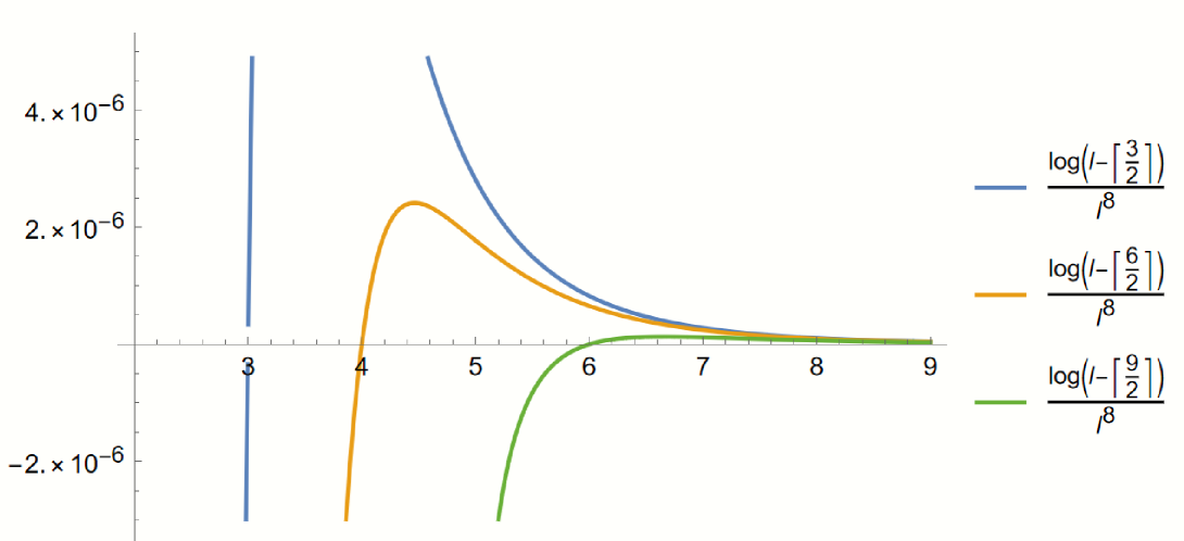
### Visual Description
\n
## Mathematical Line Graph: Logarithmic Functions with Floor Operations
### Overview
The image displays a mathematical line graph plotting three distinct functions against a common x-axis. The graph illustrates the behavior of functions involving logarithms and floor functions, scaled by a factor of \(j^8\). The curves exhibit different asymptotic behaviors and convergence patterns as the x-value increases.
### Components/Axes
- **X-Axis**: Linear scale ranging from 3 to 9, with major tick marks at integer intervals (3, 4, 5, 6, 7, 8, 9). No axis title is present.
- **Y-Axis**: Linear scale with values in scientific notation. Major tick marks are at:
- \(-2. \times 10^{-6}\)
- \(0\) (implied by the horizontal axis line)
- \(2. \times 10^{-6}\)
- \(4. \times 10^{-6}\)
No axis title is present.
- **Legend**: Positioned on the right side of the graph, vertically aligned. It contains three entries, each with a colored line segment and a corresponding mathematical expression:
1. **Blue Line**: \(\frac{\log\left(j - \left\lfloor \frac{3}{2} \right\rfloor\right)}{j^8}\)
2. **Orange Line**: \(\frac{\log\left(j - \left\lfloor \frac{6}{2} \right\rfloor\right)}{j^8}\)
3. **Green Line**: \(\frac{\log\left(j - \left\lfloor \frac{9}{2} \right\rfloor\right)}{j^8}\)
*Note: The floor function \(\lfloor x \rfloor\) denotes the greatest integer less than or equal to \(x\).*
### Detailed Analysis
**Trend Verification & Data Points:**
1. **Blue Curve** \(\left(\frac{\log(j - 1)}{j^8}\right)\):
* **Trend**: Exhibits a vertical asymptote near \(x = 3\). It descends very steeply from a high positive value, then transitions to a smooth, decreasing curve that approaches zero from above as \(x\) increases.
* **Key Points**:
* At \(x \approx 3\), the value is off the top of the chart (exceeds \(4. \times 10^{-6}\)).
* At \(x = 4\), \(y \approx 2.5 \times 10^{-6}\).
* At \(x = 5\), \(y \approx 1.0 \times 10^{-6}\).
* At \(x = 9\), \(y\) is very close to 0, approximately \(0.1 \times 10^{-6}\).
2. **Orange Curve** \(\left(\frac{\log(j - 3)}{j^8}\right)\):
* **Trend**: Starts from negative infinity near \(x = 4\) (vertical asymptote), rises sharply to a distinct maximum, then decreases smoothly, converging toward zero from above.
* **Key Points**:
* Vertical asymptote at \(x = 4\).
* Maximum value occurs at approximately \(x = 4.5\), with \(y \approx 2.4 \times 10^{-6}\).
* At \(x = 5\), \(y \approx 1.8 \times 10^{-6}\).
* At \(x = 6\), \(y \approx 0.6 \times 10^{-6}\).
* At \(x = 9\), \(y\) is very close to 0, nearly indistinguishable from the blue curve.
3. **Green Curve** \(\left(\frac{\log(j - 4)}{j^8}\right)\):
* **Trend**: Starts from negative infinity near \(x = 5\) (vertical asymptote), increases, crosses the x-axis, and then approaches zero from below, remaining negative.
* **Key Points**:
* Vertical asymptote at \(x = 5\).
* Crosses the x-axis (\(y=0\)) at approximately \(x = 6.0\).
* At \(x = 7\), \(y \approx -0.2 \times 10^{-6}\).
* At \(x = 9\), \(y\) is very close to 0 from the negative side, approximately \(-0.05 \times 10^{-6}\).
**Spatial Grounding & Convergence:**
- For \(x > 7\), all three curves converge tightly near the x-axis (\(y=0\)). The blue and orange curves approach from the positive side, while the green curve approaches from the negative side.
- The legend is placed in the right margin, with each label horizontally aligned with the tail end of its corresponding curve.
### Key Observations
1. **Asymptotic Behavior**: Each function has a vertical asymptote at a different integer value of \(x\) (3, 4, and 5 respectively), corresponding to the point where the argument of the logarithm becomes zero or negative.
2. **Domain Restriction**: The functions are only plotted for \(x\) values where the logarithm's argument is positive. For the blue curve, this is \(x > 3\); for orange, \(x > 4\); for green, \(x > 5\).
3. **Convergence**: Despite different starting points and initial behaviors, all three functions decay rapidly towards zero as \(x\) increases, due to the dominant \(j^8\) term in the denominator.
4. **Sign Difference**: The green curve is the only one that becomes and remains negative after crossing the x-axis, because \(\log(j-4)\) is negative for \(5 < j < 5\) (since \(j-4 < 1\)).
### Interpretation
This graph visualizes the comparative decay rates of three related mathematical functions. The core pattern is: **\(\frac{\log(j - c)}{j^8}\)**, where the constant \(c\) increases (1, 3, 4).
* **Effect of the Constant \(c\)**: Increasing \(c\) shifts the vertical asymptote to the right (to a higher \(x\) value) and delays the onset of the function's positive domain. It also changes the initial magnitude and sign of the function near its asymptote.
* **Dominance of the Denominator**: The \(j^8\) term in the denominator ensures that for sufficiently large \(j\) (here, \(j > 7\)), the logarithmic growth in the numerator is completely overwhelmed. This causes all functions to converge to zero, illustrating a powerful damping effect.
* **Mathematical Insight**: The graph demonstrates how a simple change in a parameter (\(c\)) within a function's definition can drastically alter its local behavior (position of asymptote, sign, initial peak) while leaving its long-term asymptotic behavior (convergence to zero) unchanged. This is a common theme in analysis and asymptotic theory.
</details>
Figure 9: Entropy of $S(n,\ell)$ for $n=8$ , $k=3,6,9$ and $\ell\rightarrow+\infty$
The definition of clustering coefficient can be found in [3]. Let $N_{v}(t)$ be the number of edges in $G_{t}$ among neighbors of $v$ , which is the number of triangles connected to the vertex $v$ . The clustering coefficient of a graph is based on a local clustering coefficient for each vertex
$$
C[v]=\frac{N_{v}(t)}{d_{G}(v)(d_{G}(v)-1)/2},
$$
If the degree of node $v$ is $0 0$ or $1$ , then we can set $C[v]=0$ . By definition, we have $0\leq C[v]\leq 1$ for $v\in V(G)$ .
The clustering coefficient for the whole graph $G$ is the average of the local values $C(v)$
$$
C(G)=\frac{1}{|V(G)|}\left(\sum_{v\in V(G)}C[v]\right).
$$
The clustering coefficient of a graph is closely related to the transitivity of a graph, as both measure the relative frequency of triangles [22, 24].
**Proposition 3.1**
*The clustering coefficient of generalized Sierpiński graph $S(n,\ell)$ is
$$
C(S(n,\ell))=\frac{\ell^{-n}\left(2\ell-2\ell^{n}+\ell^{n+1}\right)}{\ell}.
$$*
* Proof*
For any $v\in V(S(n,\ell))$ , if $v$ is a extremal vertex, then $d_{S(n,\ell)}(v)=\ell-1$ and $G[\{N(v)\}]\cong K_{\ell-1}$ , and hence
$$
C[v]=\frac{N_{v}(t)}{d_{G}(v)(d_{G}(v)-1)/2}={\binom{\ell-1}{2}}/{\binom{\ell-
1}{2}}=1.
$$
If $v$ is not a extremal vertex, then $d_{S(n,\ell)}(v)=\ell$ and $G[\{N(v)\}]\cong K_{\ell}+e$ , where $K_{\ell}+e$ is graph obtained from a complete graph $K_{\ell}$ by adding a pendent edge. Hence, we have $C[v]={\binom{\ell-1}{2}}/{\binom{\ell}{2}}=\frac{\ell-2}{\ell}$ . Since there exists $\ell$ extremal vertices in Sierpiński graph $S(n,\ell)$ , it follows that
$$
C(S(n,\ell))=\frac{1}{|V(G)|}\left(\sum_{v\in V(G)}C[v]\right)=\frac{1}{\ell^{
n}}\left({\ell\times 1+(\ell^{n}-\ell)\frac{\ell-2}{\ell}}\right)=\frac{\ell^{
-n}\left(2\ell-2\ell^{n}+\ell^{n+1}\right)}{\ell}
$$
∎
<details>
<summary>x6.png Details</summary>
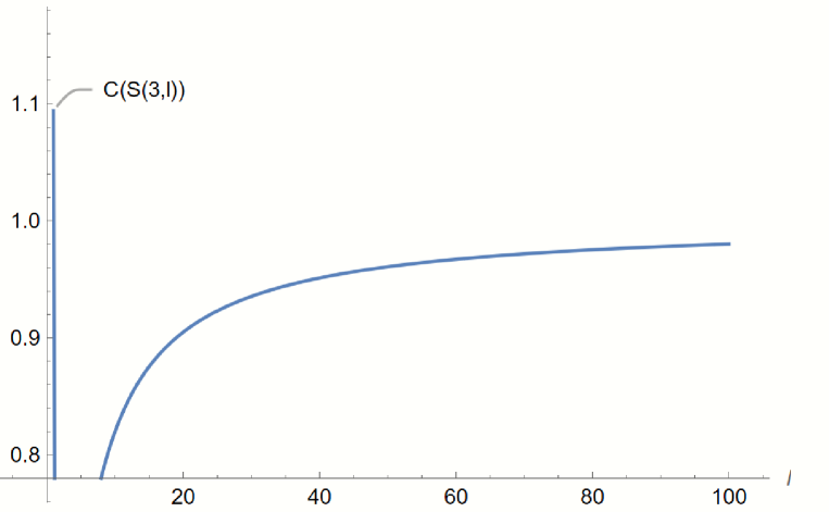
### Visual Description
## Line Graph: Function C(S(3,l)) vs. Parameter l
### Overview
The image displays a 2D line graph plotting a single mathematical function. The graph shows the relationship between a dependent variable, labeled as `C(S(3,l))`, and an independent variable, labeled `l`. The curve demonstrates a clear asymptotic growth pattern.
### Components/Axes
* **X-Axis (Horizontal):**
* **Label:** `l` (located at the far right end of the axis).
* **Scale:** Linear scale from 0 to 100.
* **Major Tick Marks & Labels:** 20, 40, 60, 80, 100.
* **Y-Axis (Vertical):**
* **Label:** No explicit axis title is present. The values represent the output of the function `C(S(3,l))`.
* **Scale:** Linear scale from approximately 0.8 to 1.1.
* **Major Tick Marks & Labels:** 0.8, 0.9, 1.0, 1.1.
* **Data Series:**
* **Label:** `C(S(3,l))` (positioned in the top-left quadrant, with a leader line pointing to the start of the curve).
* **Visual Representation:** A single, solid blue line.
* **Spatial Layout:** The plot area is framed by the axes. The function label is placed near the top-left corner of the plot area, with its leader line indicating the curve's origin point near the y-axis.
### Detailed Analysis
* **Trend Verification:** The blue line representing `C(S(3,l))` exhibits a steep, concave-down increase for low values of `l`, which gradually flattens out, approaching a horizontal asymptote as `l` increases. The slope is positive but decreasing throughout the plotted range.
* **Data Point Extraction (Approximate):**
* At `l ≈ 0`, `C(S(3,l)) ≈ 0.80` (the curve appears to start at or just above the 0.8 mark on the y-axis).
* At `l = 20`, `C(S(3,l)) ≈ 0.92`.
* At `l = 40`, `C(S(3,l)) ≈ 0.96`.
* At `l = 60`, `C(S(3,l)) ≈ 0.97`.
* At `l = 80`, `C(S(3,l)) ≈ 0.98`.
* At `l = 100`, `C(S(3,l)) ≈ 0.985` (the value is very close to, but still slightly below, 1.0).
### Key Observations
1. **Asymptotic Behavior:** The function `C(S(3,l))` appears to approach a limiting value (asymptote) of approximately 1.0 as `l` tends towards infinity. The growth rate slows significantly after `l=40`.
2. **Initial Steep Rise:** The most dramatic change in the function's value occurs for `l` between 0 and approximately 20.
3. **Monotonic Increase:** The function is strictly increasing over the entire displayed domain (`l` from 0 to 100).
4. **No Legend Required:** As there is only one data series, the direct label `C(S(3,l))` with a leader line serves as the legend.
### Interpretation
This graph visualizes the behavior of a function `C` that depends on a parameter `l`, likely through an intermediate structure or state `S(3,l)`. The notation suggests `S` might be a function or process taking arguments `3` and `l`.
The data demonstrates a classic pattern of **diminishing returns** or **saturation**. The output `C` increases rapidly with initial increases in `l`, but each subsequent unit increase in `l` yields a smaller and smaller increase in `C`. This is characteristic of many natural and mathematical phenomena, such as learning curves, chemical reaction rates approaching equilibrium, or the output of a system with a fixed capacity.
The key takeaway is that the system or property measured by `C` becomes increasingly less sensitive to the parameter `l` as `l` grows large. To achieve a value of `C` very close to 1.0, an infinitely large `l` would theoretically be required. The graph provides a quantitative view of this convergence, showing that by `l=100`, the function has already reached over 98% of its apparent asymptotic limit.
</details>
Figure 10: The Function of $C_{S(3,l)}$
<details>
<summary>x7.png Details</summary>

### Visual Description
## Line Graph: D(S(n,l)) vs. l
### Overview
The image displays a 2D line graph plotting a single data series. The graph shows a function labeled `D(S(n,l))` on the y-axis against a variable `l` on the x-axis. The curve demonstrates a clear, accelerating upward trend, suggesting a relationship of exponential or high-order polynomial growth.
### Components/Axes
* **X-Axis (Horizontal):**
* **Label:** `l` (lowercase 'L').
* **Scale:** Linear scale.
* **Tick Markers:** Major ticks are present at intervals of 2, labeled: `2`, `4`, `6`, `8`, `10`, `12`, `14`, `16`.
* **Y-Axis (Vertical):**
* **Label:** Implicitly defined by the function `D(S(n,l))` plotted on the graph.
* **Scale:** Linear scale.
* **Tick Markers:** Major ticks are present at intervals of 5,000, labeled: `0`, `5 000`, `10 000`, `15 000`, `20 000`, `25 000`, `30 000`. The space in the numbers (e.g., "5 000") is a thousands separator.
* **Data Series:**
* **Label:** `D(S(n,l))`. This label is positioned in the top-right quadrant of the chart area, near the end of the plotted line.
* **Visual Representation:** A single, solid blue line.
* **Legend/Key:** There is no separate legend box. The data series is identified by the direct label `D(S(n,l))` placed adjacent to the line's endpoint.
### Detailed Analysis
* **Trend Verification:** The blue line representing `D(S(n,l))` exhibits a monotonic, convex upward slope. It begins nearly flat and then curves sharply upward, indicating that the rate of increase itself increases as `l` grows.
* **Data Point Extraction (Approximate):**
* For `l` values from 2 to approximately 8, the y-value remains very close to 0 (likely < 100).
* At `l = 10`, the y-value is approximately `1,000`.
* At `l = 12`, the y-value is approximately `5,000`.
* At `l = 14`, the y-value is approximately `25,000`.
* The line terminates just past `l = 14`, at a y-value of approximately `26,000` to `27,000`. The label `D(S(n,l))` is placed at this endpoint.
### Key Observations
1. **Exponential-like Growth:** The most prominent feature is the dramatic, non-linear increase in the function's value. The growth is negligible for low `l` and becomes extremely rapid after `l=10`.
2. **Threshold Behavior:** There appears to be a critical point or threshold around `l=10`, after which the function's output escalates quickly.
3. **Single Variable Focus:** The graph isolates the relationship between `D(S(n,l))` and `l`. The parameters `n` and `S` within the function notation are held constant or are implicit for this specific plot.
### Interpretation
This graph visually demonstrates a computational or combinatorial complexity relationship. The notation `D(S(n,l))` is suggestive of a function `D` (perhaps representing "distance," "dimension," or "difficulty") applied to a structure `S` parameterized by `n` and `l`.
* **What the data suggests:** The function `D` grows very slowly with respect to `l` initially, but after a certain point (`l ≈ 10`), it enters a regime of explosive growth. This is characteristic of problems with exponential time complexity or state spaces that expand rapidly with input size.
* **How elements relate:** The x-axis (`l`) is the independent variable, likely representing a size, length, or level parameter. The y-axis shows the dependent cost or magnitude. The curve's shape is the core message: small increases in `l` beyond a threshold lead to massive increases in `D`.
* **Notable implications:** If this represents an algorithm's resource usage (time, memory), it indicates the algorithm becomes impractical for `l > 12`. If it represents a system's capacity or a mathematical property, it shows a phase transition or a limit to scalability. The graph serves as a warning about the "curse of dimensionality" or the cost of increasing complexity in the parameter `l`.
</details>
Figure 11: The diameter of $S(n,\ell)$
**Theorem 3.2**
*[21] The diameter of $S(n,\ell)$ is $Diam(S(n,\ell))=2^{\ell}-1$ ;*
For network properties of Sierpiński graph $S(n,\ell)$ , the the diameter function can be seen in Figure 11 and its clustering coefficient is closely related to $1$ when $\ell\longrightarrow\infty$ ; see Figure 11, which implies that the Sierpiński graph $S(n,\ell)$ is a hight transitivity graph.
## 4 Acknowledgments
The authors would like to thank the anonymous referee for the careful reading of the manuscript and the numerous helpful suggestions and comments.
## References
- [1] J.A. Bondy, U.S.R. Murty, Graph Theory, GTM 244, Springer, 2008.
- [2] R. Burton, R. Pemantle, Local characteristics, entropy and limit theorems for spanning trees and domino tilings via transfer-impedances, Ann. Prob. 21 (1993), 1329–1371.
- [3] B. Bollobás, O.M. Riordan, Mathematical results on scale-free random graphs, in: S. Bornholdt, H.G. Schuster (Eds.), Handbook of Graphs and Networks: From the Genome to the Internet, Wiley-VCH, Berlin, 2003, 1–34.
- [4] G. Chartrand, F. Okamoto, P. Zhang, Rainbow trees in graphs and generalized connectivity, Networks 55(4) (2010), 360–367.
- [5] B.L. Chen, K.C. Huange, On the Line $k$ -arboricity of $K_{n}$ and $K_{n,n}$ , Discrete Math. 254 (2002), 83–87.
- [6] X. Cheng, D. Du, Steiner trees in Industry, Kluwer Academic Publisher, Dordrecht, 2001.
- [7] M. Dehmer, F. Emmert-Streib, Z. Chen, X. Li, and Y. Shi, Mathematical foundations and applications of graph entropy, John Wiley $\&$ Sons. (2017).
- [8] D. Du, X. Hu, Steiner tree problems in computer communication networks, World Scientific, 2008.
- [9] C. Hao, W. Yang, The generalized connectivity of data center networks. Parall. Proce. Lett. 29 (2019), 1950007.
- [10] J. Gu, J. Fan, Q. Ye, L. Xi, Mean geodesic distance of the level- $n$ Sierpiński gasket, J. Math. Anal. Appl. 508(1) (2022), 125853.
- [11] S. Klavžar, U. Milutinović, Graphs $S(n,k)$ and a variant of tower of hanoi problem, Czechoslovak Math. J. 122(47) (1997), 95–104.
- [12] H. Li, X. Li, and Y. Sun, The generalied $3$ -connectivity of Cartesian product graphs, Discrete Math. Theor. Comput. Sci. 14(1) (2012), 43–54.
- [13] H. Li, Y. Ma, W. Yang, Y. Wang, The generalized $3$ -connectivity of graph products, Appl. Math. Comput. 295 (2017), 77–83.
- [14] S. Li, J. Tu, C. Yu, The generalized $3$ -connectivity of star graphs and bubble-sort graphs, Appl. Math. Comput. 274(1) (2016), 41–46.
- [15] X. Li, Y. Mao, Generalized Connectivity of Graphs, Springer Briefs in Mathematics, Springer, Switzerland, 2016.
- [16] X. Li, Y. Mao, Y. Sun, On the generalized (edge-)connectivity of graphs, Australasian J. Combin. 58(2) (2014), 304–319.
- [17] Y. Li, Y. Mao, Z. Wang, Z. Wei, Generalized connectivity of some total graphs, Czechoslovak Math. J. 71 (2021), 623–640.
- [18] C. Li, S. Lin, S. Li, The $4$ -set tree connectivity of $(n,k)$ -star networks, Theor. Comput. Sci. 844 (2020), 81–86.
- [19] S. Lin, Q. Zhang, The generalized $4$ -connectivity of hypercubes. Discrete Appl. Math. 220 (2017), 60–67.
- [20] H. Li, X. Li, Y. Sun, The generalized $3$ -connectivity of Cartesian product graphs, Discrete Math. Theor. Comput. Sci. 14 (2012), 43–54.
- [21] D. Parisse, On some metric properties of the the Sierpiński graphs $S(n,\ell)$ , Ars Comb. 90 (2009), 145–160.
- [22] J. Reichardt, Structure in complex networks. Springer Science $\&$ Business Media, 2008.
- [23] A. Sahu, A. Priyadarshi, On the box-counting dimension of graphs of harmonic functions on the Sierpiński gasket. J. Math. Analy. Appl. 487(2) (2020), 124036.
- [24] X. Wang, X. LI, G. R.Chen, Introduction to Network Science. Beijing: Higher Education Press, 2012.
- [25] B. Xue, L. Zuo, G. Li, The hamiltonicity and path $t$ -coloring of Sierpiński-like graphs, Discrete Appl. Math. 160 (2012), 1822–836.
- [26] B. Xue, L. Zuo, On the linear $(n-1)$ -arboricity of $K_{n}$ , Discrete Appl. Math. 158 (2010) 1546–1550.
- [27] S. Zhao, R. Hao, L. Wu, The generalized connectivity of $(n,k)$ -bubble-sort graphs. The Comput. J. 62 (2019), 1277–1283.
- [28] S. Zhao, R. Hao, J. Wu, The generalized $3$ -connectivity of some regular networks, J. Parall. Distr. Comput. 133 (2019), 18–29.
- [29] S. Zhao, R. Hao, The generalized connectivity of alternating group graphs and $(n,k)$ -star graphs, Discrete Appl. Math. 251 (2018), 310–321.
- [30] S. Zhao, R. Hao, E. Cheng, Two kinds of generalized connectivity of dual cubes, Discrete Appl. Math. 257 (2019), 306–316.
- [31] S. Zhao, R. Hao, The generalized connectivity of alternating group graphs and $(n,k)$ -star graphs, Discrete Appl. Math. 251 (2018), 310–321.
- [32] S. Zhao, R. Hao, The generalized $4$ -connectivity of exchanged hypercubes, Applied Mathe. Comput. 347 (2019), 342–353.
- [33] S. Zhao, R. Hao, J. Wu, The generalized $4$ -connectivity of hierarchical cubic networks, Discrete Appl. Mathe., 289 (2021), 194–206.
- [34] S. Zhao, J. Chang, Z. Li, The generalized $4$ -connectivity of pancake graphs, Discrete Appl. Math. 327 (2023), 77–86.
- [35] S. Zhao, R. Hao, The generalized $4$ -connectivity of exchanged hypercubes. Appl. Math. Comput. 347 (2019), 342–353.