2310.17004

# Improved Panning on Non-Equidistant Loudspeakers with Direct Sound Level Compensation **Authors**: Jan-Hendrik Hanschke, Daniel Arteaga, Giulio Cengarle, Joshua Lando, Mark R. P. Thomas, Alan Seefeldt ## Improved Panning on Non-Equidistant Loudspeakers with Direct Sound Level Compensation Jan-Hendrik Hanschke, Daniel Arteaga, Giulio Cengarle, Joshua Lando, Mark R.P. Thomas, and Alan Seefeldt 1 1 Dolby Laboratories Correspondence should be addressed to Jan-Hendrik Hanschke ( janhendrikhanschke@ieee.org ) ## ABSTRACT Loudspeaker rendering techniques that create phantom sound sources often assume an equidistant loudspeaker layout. Typical home setups might not fulfill this condition as loudspeakers deviate from canonical positions, thus requiring a corresponding calibration. The standard approach is to compensate for delays and to match the loudness of each loudspeaker at the listener's location. It was found that a shift of the phantom image occurs when this calibration procedure is applied and one of a pair of loudspeakers is significantly closer to the listener than the other. In this paper, a novel approach to panning on non-equidistant loudspeaker layouts is presented whereby the panning position is governed by the direct sound and the perceived loudness is governed by the full impulse response. Subjective listening tests are presented that validate the approach and quantify the perceived effect of the compensation. In a setup where the standard calibration leads to an average error of 10 ◦ , the proposed direct sound compensation largely returns the phantom source to its intended position. ## 1 Introduction In stereo or multichannel loudspeaker setups, a virtual or phantom source is a sound that appears to emanate from a position other than the physical loudspeaker locations [1]. The most common rendering techniques for creating such phantom sources are based on stereo amplitude panning and their multichannel extensions (e.g., vector-base amplitude panning [2], dual/triple balance amplitude panning [3], distance-based amplitude panning [4]). These panning methods distribute the source signal among several loudspeakers, assigning a gain to each loudspeaker so that the resulting sound mixture creates the illusion of a phantom sound source coming from the intended direction. Amplitude panning techniques are commonly used in professional content creation tools for cinema, music and multimedia. With traditional channel-based formats, panning to channels takes place at the content creation side, addressing a small discrete set of canonical playback configurations (e.g., stereo, 5.1, etc.). These channel-based renderings are then played back on consumer systems where the loudspeaker positions may deviate from the canonical locations, causing a mismatch in angle and perceived level. These inaccuracies result in a shift of the perceived position of a phantom source with respect to the intended position. Object-based audio [5], which utilizes a renderer in the playback device and knowledge of the loudspeaker layout, opens the door to modifying relative gains of individual sources based on the knowledge of actual loudspeaker location and acoustic characteristics of the playback system. So far, most rendering techniques, including those that allow for flexible positioning of loudspeakers and process object-based audio, depend only on the angular position of the loudspeakers relative to the listener. The distance between each loudspeaker and the listening position is assumed to be equal, even if in common home setups that might not hold true. In case of unequal distances, the state of the art approach is to time align and loudness match the different loudspeakers [2], with the loudness estimated from the full room response of each loudspeaker, which we will refer to as full response compensation (FRC). In the authors' experience, this calibration approach fails when rendering content to layouts with non-equidistant loudspeakers, causing the phantom source to be systematically pulled towards the closest loudspeaker(s). Upon a more thorough reflection with regards to the position of a phantom source, the procedure of loudness matching seems to be at least partially at odds with the well established psychoacoustic principle of the Haas or precedence effect [6, 7]. When a sound is followed by a delayed version of itself with a time delay of approximately 1 ms or more (but less than the echo threshold), a single auditory event is perceived from the direction of the first arriving wavefront. As a consequence, the perceived direction of a single physical sound source in a room is dominated by sound on the direct path from the source to the listener, not by later arriving room reflections [8]. For time delays smaller than approximately 1 ms, the related summing localization principle [9] states that multiple wavefronts of sound fuse into a phantom source whose perceived direction is a combination of those for each wavefront. When considering panning across multiple time-aligned loudspeakers, this gives strong indication that the quantity determining the virtual source location is the direct sound from each loudspeaker, possibly including early reflections arriving before 1 ms, and not the total sound loudness contained in the entire reverberation tail. Although some literature in the context of equalization hints at the possibility that the direct sound plays a dominant role in the localization and timbre perception of sound [10, 11], and another study uses the anechoic decay as a simplified room model in a panning function [12], we are not aware of systematic studies of this phenomenon in the context of loudspeaker rendering, nor of any practical implementations. We study and propose a modified panning approach for non-equidistant loudspeakers based on the combined contributions of the direct sound from multiple loudspeakers, and show empirically that it leads to improved phantom source localization accuracy. In order to achieve loudness consistency across multiple phantom source locations, the total response of the loudspeakers is simultaneously considered. The paper is organized as follows: In Sec. 2 we introduce relevant quantities based on the sound decay model and explain the full response compensation method for level and delay compensation. Sec. 3 then covers the proposed approach to restore the intended phantom source position based on the direct sound contribution while maintaining loudness consistency. In Sec. 4 we describe a subjective listening test to validate the proposed approach and in Sec. 5 we present its results. These results and the main outcomes of the paper are discussed in Sec. 6. ## 2 Fundamentals ## 2.1 Distance-based level decay of loudspeakers in reverberant rooms As a loudspeaker plays a signal in a room, the direct sound-the sound traveling on the shortest path from the loudspeaker to the listener-is quickly followed by multiple, spatially diverse, indirect reflections with increasing temporal density, often referred to as the diffuse sound field. The direct sound intensity decays as the squared distance from the loudspeakers. The corresponding direct sound level for each loudspeaker, L DS i in decibel scale is <!-- formula-not-decoded --> where Pi is the acoustic power of a source i , Qi its directivity factor in the direction of the listener, and di is the distance to the source. The diffuse sound intensity is almost constant, depends upon the room characteristics and varies little with source and receiver position, orientation, or distance. The distance at which direct and diffuse intensities are equal is commonly referred to as the critical distance Dc . The overall loudness at the listening position for a given loudspeaker can be inferred by assuming the total sound as the sum of direct sound and diffuse sound field. On axis, the loudness can be estimated from the total sound intensity in decibel scale as <!-- formula-not-decoded --> In practice Li can also be obtained from the measurement with a sound level meter, e.g. when capturing pink noise. An equivalent calibration can be achieved through the acquisition and analysis of impulse responses (IRs). The loudness can be estimated from the RMS value of the IR hi ( t ) , with optional weighting filters applied wA ( t ) , for example A-weighting: <!-- formula-not-decoded --> The direct sound level L DS i for each loudspeaker cannot be measured with a sound level meter. One option to obtain it is to use the room-independent model per (1). It can also be estimated by multiplying measured impulse responses with a time window that vanishes beyond a certain truncation time t after the arrival of the first peak. Using a small, fixed truncation time has the drawback that frequencies approximately lower than the inverse truncation time cannot be adequately represented. 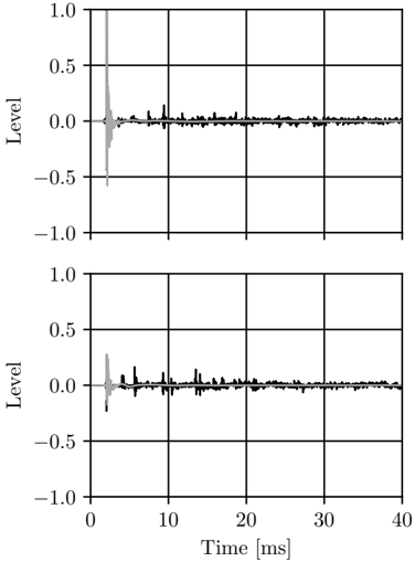A frequency-dependent truncation (FDT) kernel k ( n ) [13] may be used to estimate the direct sound portion of the impulse response: <!-- formula-not-decoded --> The frequency-dependent truncation filter truncates all frequency components of the impulse response to a time t or smaller. Most commonly, it truncates the lowest frequency under consideration to a time t and higher frequencies to a time smaller than t . This approach has the advantage of providing a better representation of the lower frequencies without compromising the truncation of the impulse response at higher frequencies. Fig. 1 shows examples of FDT applied to impulse responses of non-equidistant loudspeakers in a reverberant room. The corresponding direct sound level L DS i can be estimated by substituting hi for h DS i in (3). ## 2.2 Full response compensation (FRC) of non-equidistant loudspeakers The state of the art calibration approach involves loudness matching and loudspeaker time alignment. Loudness matching ensures that each loudspeaker produces the same loudness at the listening position when fed with a reference signal. Given a set of loudspeakers producing a loudness Li at the listening position, the loudness compensation D Li for each loudspeaker is <!-- formula-not-decoded --> where L ref is a pre-established reference level. The loudness compensation gains are given by 10 D Li / 20 . To maintain loudness consistency, the gains gi produced by a panner are usually normalized so that the loudness of the phantom sound source is equal to the loudness of the corresponding sound source when emanating only from a single loudspeaker. For loudness-matched setups, this requires the following relationship be satisfied: <!-- formula-not-decoded --> with p usually between 1 and 2. The common sine/cosine pairwise panning law is an example which satisfies the above condition for p = 2. However, any panning law can meet this requirement through normalization. Fig. 1: Measured IR (black line) for a loudspeaker at 1 . 5 m (top) vs. 3 m (bottom) distance, leading to a theoretical direct sound decay of 6 dB. Analysis of IRs with Frequency Dependent Truncation (grey line) shows a 6 . 3 dB level difference (pink- and A-weighted) in direct sound vs. 3 . 0 dB in overall sound (black line) between near and far loudspeaker. <details> <summary>Image 1 Details</summary>  ### Visual Description \n ## Chart: Signal Level vs. Time ### Overview The image presents two identical line charts displaying signal level as a function of time. Both charts show a rapid initial drop in signal level followed by a stabilization around zero, with some minor fluctuations. The charts appear to represent the same data, potentially showing replicates or different conditions. ### Components/Axes * **X-axis:** Time [ms], ranging from 0 to 40 milliseconds. The axis is marked with increments of 10 ms. * **Y-axis:** Level, ranging from -1.0 to 1.0. The axis is marked with increments of 0.5. * **Data Series:** A single black line is present in each chart, representing the signal level over time. * **Gridlines:** A grid is overlaid on both charts, aiding in the reading of values. ### Detailed Analysis Both charts exhibit similar behavior. **Chart 1:** * The signal level starts at approximately 0.2 at time 0 ms. * There is a rapid decrease in signal level, reaching a minimum of approximately -0.75 at around 1.5 ms. * Following the initial drop, the signal level oscillates around 0, with fluctuations between approximately -0.2 and 0.2. * From approximately 5 ms to 40 ms, the signal level remains relatively stable, fluctuating within a narrow range around 0. **Chart 2:** * The signal level starts at approximately 0.15 at time 0 ms. * There is a rapid decrease in signal level, reaching a minimum of approximately -0.7 at around 1.5 ms. * Following the initial drop, the signal level oscillates around 0, with fluctuations between approximately -0.2 and 0.2. * From approximately 5 ms to 40 ms, the signal level remains relatively stable, fluctuating within a narrow range around 0. ### Key Observations * Both charts show a very similar initial drop in signal level. * The signal stabilizes around zero after the initial transient. * The fluctuations after the initial drop are relatively small in amplitude. * There is a slight difference in the initial signal level between the two charts. ### Interpretation The charts likely represent a signal response to a step input or a similar triggering event. The initial drop suggests a rapid change in signal state, followed by a settling period where the signal fluctuates around a baseline level of zero. The similarity between the two charts suggests the system is behaving consistently. The slight difference in initial signal level could be due to minor variations in experimental conditions or measurement noise. The data suggests a fast response time (less than 5 ms) and a stable baseline after the initial transient. The charts do not provide information about the nature of the signal or the system generating it, only its temporal behavior. </details> Loudspeaker time alignment consists of adding time delays to the closer loudspeakers so that all loudspeaker signals arrive at the listening position at the same time. The delays D t i applied to each loudspeaker are <!-- formula-not-decoded --> where c is the speed of sound and d ref is a reference distance, usually the distance to the most distant loudspeaker. ## 3 Improved panning on non-equidistant loudspeakers As mentioned in the introduction, we observed that the phantom source is systematically pulled towards the closest loudspeakers when using the full response compensation approach outlined in Sect. 2.2. Here we propose an alternate procedure that restores the phantom source to its intended position by matching the direct sound from each loudspeaker and preserving the correct loudness by matching levels derived from the full response. ## 3.1 Improved phantom source location: direct sound compensation (DSC) Given a set of loudspeakers whose direct sound is characterized by a level L DS i as measured in decibels from the listener position, the direct sound compensation for each loudspeaker D Li is <!-- formula-not-decoded --> where L DS ref is a reference direct sound level. The directsound compensation gains are 10 D L DS i / 20 . We assume that the loudspeaker calibration according to the full response compensation procedure outlined in Sec. 2.2 is already in place. To preserve the correct phantom source locations, the direct sound compensation needs to be applied to the gains and the effect of loudness compensation needs to be undone. Therefore, the panning gains gi coming from the amplitude panning algorithm are modified as follows: <!-- formula-not-decoded --> ## 3.2 Loudness correction The application of (9) will lead to phantom source images in their correct location, but the loudness of each one of the phantom sources will generally not be correct as the perception of loudness is governed by the level of the entire room response, and not only by the direct sound. 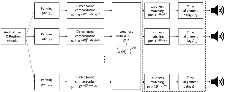To recover the correct loudness of the phantom sound sources, gains g ′ i coming from the process of direct sound compensation are normalized to meet the condition in (6): <!-- formula-not-decoded --> The complete system, a combination of the full response compensation approach with the additional direct sound compensation gain per source object is depicted in Fig. 2. Combining the gains stages from (9) and (10) along with the full response loudness compensation gains 10 D Li / 20 , the combined gains Gi for a source fed to each loudspeaker are <!-- formula-not-decoded --> Should the method outlined here be applied to a loudspeaker setup calibrated in a different way than the state of the art FRC procedure, the specific details in Fig. 2, as well as (9) and (10), would change, but (11) above would still be valid. ## 3.3 Practical implementation From (11) the final panning gains are clearly dependent on the specifics of the loudspeaker layout, but more critically they are dependent in a manner that varies with phantom source location. This may be appreciated by noting that the denominator of (11) is a function of all the unmodified amplitude panning gains gi across all loudspeakers and will therefore in general be different for different phantom source locations. As such, a practical implementation requires a renderat-playback-time approach, where the panning gains of each source are applied independently based on the actual loudspeaker layout before mixing together into loudspeaker feeds. This allows for the accounting of direct sound and overall level differences on a per-source basis. This approach works naturally with object-based audio formats but can also be applied to pre-rendered channel-based formats by treating each channel as a "static object" with an assumed canonical playback position. This paper presents a broadband analysis and compensation of direct sound and overall loudness. All considerations can be extended to frequency dependent, narrowband calibration based on measurements in the listening room. ## 4 Experimental methods To formally confirm the theoretical and practical findings, a two-part listening test was conducted, isolating the audio attributes of interest respectively: one part focused on the spatial location of phantom sound sources described in Sec. 4.1; the second part targeted Fig. 2: System diagram of a panning algorithm enhanced by direct sound compensation, followed by full response loudness compensation and time alignment (dotted box). <details> <summary>Image 2 Details</summary>  ### Visual Description ## Diagram: Spatial Audio Processing Pipeline ### Overview The image depicts a diagram illustrating a spatial audio processing pipeline. The pipeline takes "Audio Object & Position Metadata" as input and processes it through a series of stages – Panning, Direct Sound Compensation, Loudness Normalization/Matching, and Time Alignment – to produce an audio output represented by a speaker icon. The diagram shows this process repeated for multiple audio objects, indicated by the ellipsis (...). ### Components/Axes The diagram consists of the following components, arranged in a linear flow from left to right: * **Input:** "Audio Object & Position Metadata" * **Panning:** Gain denoted as *g_i*, where *i* ranges from 1 to *n*. * **Direct Sound Compensation:** Gain calculated as 10^{(ΔL_i² - ΔL₁) / 20}. * **Loudness Normalization/Matching:** The first instance has a gain of 1 / (Σ|g_j|^p)^1/p. Subsequent instances have a gain of 10^{ΔL_i / 20}. * **Time Alignment:** Delay denoted as Δt_i, where *i* ranges from 1 to *n*. * **Output:** Speaker icon representing the audio output. * **Ellipsis:** Indicates repetition of the processing stages for multiple audio objects. ### Detailed Analysis or Content Details The diagram illustrates a parallel processing structure. Each audio object's metadata is processed independently through the pipeline. 1. **Audio Object & Position Metadata:** This is the initial input to the system. 2. **Panning (g_i):** The audio signal is panned using a gain *g_i*. 3. **Direct Sound Compensation:** A gain is applied to compensate for direct sound differences, calculated as 10^{(ΔL_i² - ΔL₁) / 20}. ΔL_i and ΔL₁ represent some form of level difference. 4. **Loudness Normalization/Matching:** * For the first audio object (i=1), a loudness normalization gain is applied: 1 / (Σ|g_j|^p)^1/p. The summation (Σ) is over all audio objects *j*. The parameter *p* is not defined. * For subsequent audio objects (i > 1), a loudness matching gain is applied: 10^{ΔL_i / 20}. 5. **Time Alignment (Δt_i):** A time delay Δt_i is applied to each audio object. 6. **Output:** The processed audio signal is outputted through a speaker. The ellipsis indicates that this process is repeated for *n* audio objects. ### Key Observations * The diagram highlights a parallel processing architecture for spatial audio rendering. * The loudness normalization/matching stage appears to be crucial for maintaining consistent loudness levels across different audio objects. * The use of gains and delays suggests that the system is manipulating the amplitude and timing of the audio signals to create a spatial impression. * The formula for Direct Sound Compensation uses a squared difference (ΔL_i²), which could emphasize larger level differences. * The parameter *p* in the loudness normalization formula is undefined, suggesting it might be a tunable parameter. ### Interpretation This diagram represents a simplified model of a spatial audio rendering system. The core idea is to take audio objects with positional information and transform them into signals that, when played through multiple speakers, create a sense of spatial localization. The panning stage positions the sound source in the stereo field. The direct sound compensation likely aims to account for differences in the direct sound level between the listener and each speaker. The loudness normalization/matching stage ensures that all audio objects are perceived at roughly the same loudness, regardless of their distance or position. Finally, the time alignment stage introduces delays to account for the different travel times of sound from each source to the listener, further enhancing the spatial impression. The use of gains and delays suggests that the system is based on amplitude panning and time-delay stereophony techniques. The ellipsis indicates that the system can handle multiple audio objects simultaneously, creating a more immersive and realistic soundscape. The undefined parameter *p* suggests a degree of flexibility in the loudness normalization process, potentially allowing for different perceptual weighting schemes. </details> the validation of applied loudness correction described in Sec. 4.2. 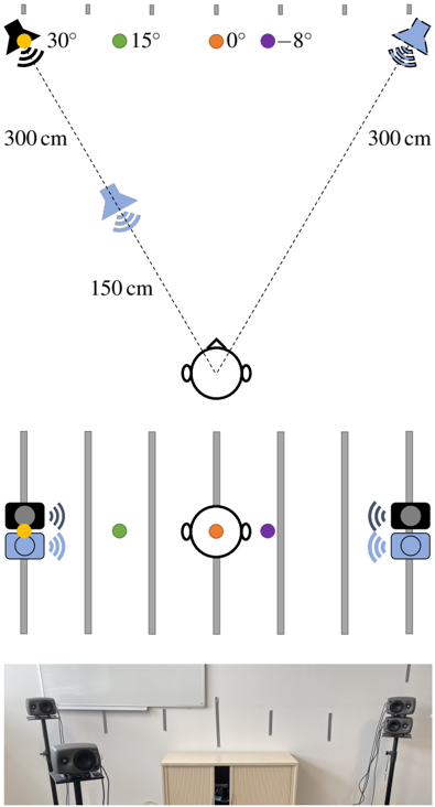The physical audio system was shared between the two experiments and was set up in an acoustically untreated room, matching typical living room conditions. It consisted of two stereo setups each with loudspeakers at 30 ◦ and -30 ◦ . One setup had the two loudspeakers placed equidistant at 300 cm with a height of 120 cm. The other one had the left loudspeaker at half the distance (150 cm) of the right one (300 cm). Both loudspeakers for this non-equidistant setup were at a height of 104 cm. A small loudspeaker model (Genelec 8020) was chosen to minimize acoustic impact in the form of occlusion and scattering from the lower, closer loudspeaker on the one behind it. The average ear height of the seated participants was 112 cm, in the middle between the two systems, ensuring an undisturbed acoustic path of both loudspeaker setups to the listener. Fig. 3 shows a schematic view of the listening test setup along with a picture of the actual setup. Loudspeakers are delay and level aligned according to the FRC calibration procedure based on measured impulse responses. The corresponding IRs, which were also analyzed by FDT to ascertain the direct sound levels, can be seen in Fig. 1. These direct sound levels matched the inverse square law (1). The listening test was realized using the webMUSHRA software [14]. There were 16 participants (13 male, 3 female) with an average age of 39.4 years. In a questionnaire 56% stated that they are audio professionals, 43% had past listening test experience and 19% claimed to be expert spatial audio listeners. 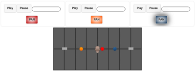## 4.1 Localization test In the first listening test, participants were asked to evaluate the perceived angle of phantom sound sources. As shown in Fig. 4 three conditions were presented on each page of the listening test software. Each of these conditions used the same mono source content panned to an intended angle using three different panning approaches. For all three the underlying panning law was sin/cos panning. Intended source angles were 30 ◦ , 15 ◦ , 0 ◦ and -8 ◦ . The REF condition utilized the equidistant loudspeakers. The FRC condition refers to the non-equidistant loudspeakers which are delay and level aligned (see Sec. 2.2). DSC refers to the panning on the same system according to the methodology described in Sec. 3. The mono source content was a selection of a pop song, pink noise bursts, female speech, drums, and harpsichord samples. The UI position of each stimulus was initialized to a random position; similarly the order of all stimuli was randomized. The participants were instructed to switch between the three conditions on each page and drag and drop little spheres to the desired positions indicating the perceived azimuth location of the phantom sound sources. 10 ◦ step markers on the Fig. 3: A schematic top and front view of the listening test setup along with a picture of the actual setup. Four dots indicate the intended phantom sources angle at 30 ◦ , 15 ◦ , 0 ◦ and -8 ◦ . 10 degree markers help the participants connect reality to the listening test interface. <details> <summary>Image 3 Details</summary>  ### Visual Description \n ## Diagram: Spatial Audio Setup ### Overview This diagram illustrates a spatial audio setup with four speakers positioned around a central listening position. It depicts the speaker angles, distances, and a photograph of the physical setup. The diagram is divided into three main sections: a top-down view with angles and distances, a simplified representation of speaker positions, and a photograph of the actual setup. ### Components/Axes * **Speakers:** Represented by black squares with a speaker icon. * **Listening Position:** Represented by a head silhouette with concentric circles indicating sound reception. * **Angles:** 30°, 15°, 0°, -8° (associated with each speaker). * **Distances:** 300 cm (distance from two speakers to the listening position), 150 cm (distance from the central speaker to the listening position). * **Color Coding:** * Black: 30° speaker * Green: 15° speaker * Orange: 0° speaker * Purple: -8° speaker * **Vertical Lines:** Representing the physical placement of the speakers. ### Detailed Analysis / Content Details The diagram shows a top-down view of the speaker arrangement. * **Speaker 1 (Black, 30°):** Located on the top-left, emitting sound waves at a 30-degree angle. Distance to listening position is 300 cm. * **Speaker 2 (Green, 15°):** Located on the top-center, emitting sound waves at a 15-degree angle. Distance to listening position is 300 cm. * **Speaker 3 (Orange, 0°):** Located in the center, emitting sound waves at a 0-degree angle. Distance to listening position is 150 cm. * **Speaker 4 (Purple, -8°):** Located on the top-right, emitting sound waves at a -8-degree angle. Distance to listening position is 300 cm. The simplified representation below the top-down view shows the speakers as colored circles corresponding to their angles, positioned along vertical lines. The listening position is represented by a head silhouette with concentric circles. The bottom section is a photograph of the physical setup. It shows four speakers on stands, positioned in a room. A cabinet is visible in the center of the room. ### Key Observations * The speakers are not equidistant from the listening position. The central speaker is closer (150 cm) than the other three (300 cm). * The angles suggest a wide soundstage, covering from -8° to 30°. * The color coding is consistent throughout the diagram, linking speaker position, angle, and representation. ### Interpretation This diagram details the setup for a spatial audio experiment or demonstration. The varying distances and angles of the speakers are likely intended to create a specific auditory experience for the listener. The central speaker at a closer distance may serve as a primary sound source, while the surrounding speakers provide spatial cues. The photograph confirms the physical arrangement matches the schematic representation. The setup appears to be designed to create a surround sound experience, with the angles and distances carefully chosen to optimize sound localization and immersion. The use of angles suggests an attempt to create a realistic sound field, potentially for virtual reality or audio testing purposes. </details> Fig. 4: Listening test interface used the localization experiment. The intended angle is shared among the three conditions per page. REF, FRC and DSC systems are rated simultaneously. <details> <summary>Image 4 Details</summary>  ### Visual Description \n ## Diagram: Control Interface with Visualization ### Overview The image depicts a control interface with three sets of "Play/Pause/Pan" buttons positioned above a grid-like visualization. The visualization contains four colored circles, likely representing tracked objects or data points, arranged within the grid. The interface appears to control the visualization, potentially allowing for playback, pausing, and panning across the grid. ### Components/Axes The image consists of the following components: * **Control Buttons:** Three sets of buttons, each containing "Play", "Pause", and "Pan" options. * **Visualization Grid:** A dark gray grid composed of vertical rectangles. * **Tracked Objects:** Four colored circles (orange, red, blue, and a lighter brown/beige) positioned within the grid. * **Sliders:** Three horizontal sliders are positioned below the "Play" and "Pause" buttons. The grid itself does not have explicit axes labels, but it appears to represent a coordinate space. ### Detailed Analysis or Content Details The image shows three identical control sets arranged horizontally. Each set has: * A "Play" button. * A "Pause" button. * A "Pan" button. The "Pan" buttons are colored differently: red, orange, and a light blue. The visualization grid is composed of approximately 10 vertical columns. The four colored circles are positioned as follows (approximate relative positions): * **Orange Circle:** Located approximately 2 columns from the left edge. * **Red Circle:** Located approximately 5 columns from the left edge, and centered vertically. * **Blue Circle:** Located approximately 8 columns from the left edge. * **Beige/Brown Circle:** Located approximately 4 columns from the left edge. The sliders are positioned below the "Play" and "Pause" buttons. They appear to be inactive or at their minimum value. ### Key Observations * The different colors of the "Pan" buttons suggest different panning modes or directions. * The positioning of the circles within the grid may represent their coordinates or locations. * The sliders likely control some aspect of the visualization or the tracked objects. * The interface appears to be designed for interactive control of the visualization. ### Interpretation This image likely represents a user interface for a tracking or monitoring system. The grid could represent a physical space, a data space, or a simulation environment. The colored circles represent objects or data points being tracked within that space. The "Play/Pause" buttons control the animation or progression of the tracking, while the "Pan" buttons allow the user to navigate the visualization. The sliders likely control parameters such as speed, zoom, or other relevant settings. The differing colors of the "Pan" buttons suggest that different panning modes are available, potentially allowing the user to pan in specific directions or focus on particular areas of the grid. The interface is designed for interactive exploration and analysis of the tracked objects or data. The image does not provide any quantitative data or specific values, but it conveys the functionality and layout of a control system. It is a visual representation of a system designed for observation and manipulation of data within a defined space. </details> wall of the room matched identical indicators in the listening test software user interface and helped the listeners to connect it to reality. Five participants were excluded from the localization test. Four of them were excluded because in more than 15% of the cases they reported a hard panning to the left loudspeaker (30 ◦ ) anchor as being located at less than 15 ◦ . Another participant was excluded due to inconsistent reporting. ## 4.2 Loudness test To validate accurate loudness correction for phantom sound sources, listeners were asked to participate in a second part of the listening test. The utilized methodology was adapted from the loudness validation test proposed in [15]. The standardized ITU BS.1534 MUSHRA [16] interface was used, where the explicit and hidden reference was a panned source on the symmetric loudspeaker layout (REF). The participants were asked to evaluate the loudness of the same phantom source panned on the non-equidistant loudspeaker setup with respect to their similarity to the reference purely with respect to loudness. Two variants of DSC panned sources were presented, depending on whether direct sound compensation included the loudness correction in (10), or not: DSC LC, with loudness correction, and DSC NO LC, without it. Furthermore, an anchor in the form of a scaled reference at -10 dB was added (ANCH). Listeners provided a rating according to the MUSHRA scale with verbal anchors of bad, poor, fair, good and excellent . Phantom sound sources were panned to 30 ◦ , 15 ◦ , 0 ◦ with the same mono content selection from the previous part of the test. To shorten the length of the test -8 ◦ was left out since the smallest differences were expected for it. One participant was excluded from the second test on the basis of evaluating more than 15% of the hidden reference cases with less than 90 points. ## 5 Experimental results The statistical analysis follows the general guidelines in ITU-R BS.1534 [16], and was done using the rstatix package in R [17, 18]. 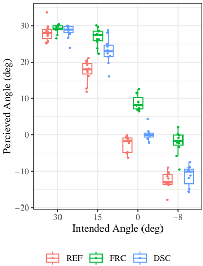Fig. 5: Localization test: perceived angular locations, as a function of the four intended angles [30 ◦ (i), 15 ◦ (ii), 0 ◦ (iii), -8 ◦ (iv)] and the test condition (REF, FRC, DSC). Dots represent the result of each one of the participants, averaged over all 5 contents items, and the box plots show the corresponding median values and interquartile range. <details> <summary>Image 5 Details</summary>  ### Visual Description ## Scatter Plot: Perceived vs. Intended Angle ### Overview This image presents a scatter plot comparing the intended angle of a stimulus to the perceived angle by a subject. The data is presented as box-and-whisker plots for three different conditions: REF, FRC, and DSC. Individual data points are also plotted as dots. The plot aims to visualize any systematic biases or distortions in angle perception. ### Components/Axes * **X-axis:** "Intended Angle (deg)" - Ranges from approximately -8 to 30 degrees. Marked at -8, 0, 15, and 30. * **Y-axis:** "Perceived Angle (deg)" - Ranges from approximately -20 to 30 degrees. * **Legend:** Located at the bottom-center of the image. * REF (Red): Represents one condition. * FRC (Green): Represents another condition. * DSC (Blue): Represents a third condition. ### Detailed Analysis The plot displays box-and-whisker plots for each condition at several intended angles. Individual data points are scattered around these box plots. **REF (Red):** * At Intended Angle = 30 deg: Perceived Angle median is approximately 27 deg, with the box extending from roughly 23 to 31 deg. Several points are above 30 deg. * At Intended Angle = 15 deg: Perceived Angle median is approximately 18 deg, with the box extending from roughly 12 to 22 deg. * At Intended Angle = 0 deg: Perceived Angle median is approximately -3 deg, with the box extending from roughly -7 to 2 deg. * At Intended Angle = -8 deg: Perceived Angle median is approximately -12 deg, with the box extending from roughly -16 to -8 deg. **FRC (Green):** * At Intended Angle = 30 deg: Perceived Angle median is approximately 30 deg, with the box extending from roughly 27 to 33 deg. * At Intended Angle = 15 deg: Perceived Angle median is approximately 11 deg, with the box extending from roughly 8 to 15 deg. * At Intended Angle = 0 deg: Perceived Angle median is approximately 8 deg, with the box extending from roughly 5 to 12 deg. * At Intended Angle = -8 deg: Perceived Angle median is approximately -2 deg, with the box extending from roughly -5 to 2 deg. **DSC (Blue):** * At Intended Angle = 30 deg: Perceived Angle median is approximately 30 deg, with the box extending from roughly 26 to 33 deg. * At Intended Angle = 15 deg: Perceived Angle median is approximately 22 deg, with the box extending from roughly 18 to 26 deg. * At Intended Angle = 0 deg: Perceived Angle median is approximately 1 deg, with the box extending from roughly -2 to 4 deg. * At Intended Angle = -8 deg: Perceived Angle median is approximately -10 deg, with the box extending from roughly -14 to -6 deg. ### Key Observations * **Underestimation:** For all three conditions, there's a general trend of underestimation of the intended angle, particularly at positive angles. The perceived angle is consistently lower than the intended angle. * **Condition Differences:** The REF condition shows the most significant underestimation at 30 degrees. The FRC and DSC conditions appear to have more accurate perception at 30 degrees. * **Negative Angle Perception:** At -8 degrees, all three conditions show a tendency to perceive the angle as more negative than intended. * **Data Spread:** The spread of data points (as indicated by the box-and-whisker plots) varies across conditions and intended angles, suggesting different levels of perceptual variability. ### Interpretation The data suggests a systematic bias in angle perception, where individuals tend to underestimate positive angles and overestimate negative angles. This bias appears to be more pronounced in the REF condition compared to the FRC and DSC conditions. This could indicate that the REF condition involves a different perceptual mechanism or a greater susceptibility to distortion. The differences between the conditions might be related to the specific experimental setup or the type of stimulus used. The spread of data points suggests individual differences in perceptual accuracy. The consistent underestimation of positive angles could be related to a cognitive tendency to centralize perceptions or a specific characteristic of the visual system. Further investigation would be needed to determine the underlying causes of these perceptual biases. </details> ## 5.1 Localization test Initially, the normality of the data was examined by means of a QQ plot, which revealed no apparent deviations from normality. A 3-way repeated measures ANOVA was conducted to examine whether the perceived angular positions were dependent on the test content. No significant interaction was revealed [ F ( 8 , 80 ) = 0 . 8, p = . 6]. Subsequently, results were averaged over the different source content items. The resulting data distribution is shown in Fig. 5, as a function of the three test conditions (REF, FRC, DSC) and the four panning angles [30 ◦ (i), 15 ◦ (ii), 0 ◦ (iii), -8 ◦ (iv)]. 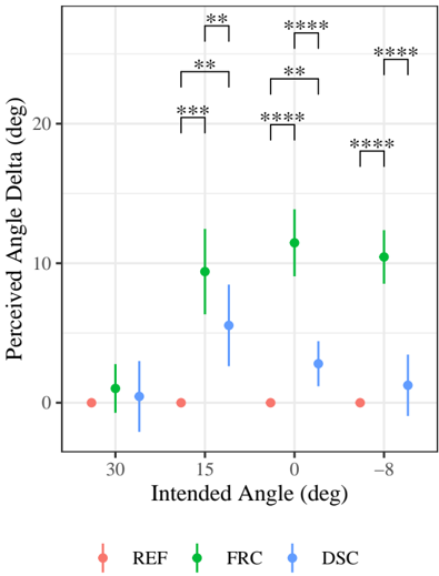The median perceived positions for the symmetric reference system Fig. 6: Localization test: Mean delta perceived angular positions relative to the reference. Dots represent the mean values and bars the confidence intervals of the mean (95% CL). The stars in the plot indicate statistically significant t -tests (adjusted for multiple comparisons). One star (*) denotes p <. 05, two stars (**) denote p <. 01, three stars (***) denote p <. 001, and four stars (****) denote p < 10 -4 . <details> <summary>Image 6 Details</summary>  ### Visual Description ## Chart: Perceived Angle Delta vs. Intended Angle ### Overview The image presents a chart illustrating the relationship between the intended angle and the perceived angle delta (in degrees) for three different conditions: REF, FRC, and DSC. The data is presented as point plots with error bars, and statistical significance is indicated by bracketed asterisks above the data points. ### Components/Axes * **X-axis:** "Intended Angle (deg)" with markers at -30, -15, 0, -8. * **Y-axis:** "Perceived Angle Delta (deg)" ranging from approximately -5 to 25. * **Data Series:** * REF (Red): Represented by red circles with error bars. * FRC (Green): Represented by green triangles with error bars. * DSC (Blue): Represented by blue diamonds with error bars. * **Legend:** Located at the bottom center of the chart, labeling the data series with their corresponding colors and symbols. * **Significance Brackets:** Black brackets with asterisks indicating statistical significance between conditions at each intended angle. The number of asterisks indicates the level of significance (e.g., **, ***, ****). ### Detailed Analysis The chart displays data points for each condition (REF, FRC, DSC) at each intended angle (-30, -15, 0, -8). The error bars represent the variability around each data point. * **Intended Angle -30 deg:** * REF: Approximately -1.5 deg ± 2 deg. * FRC: Approximately 2.5 deg ± 2 deg. * DSC: Approximately -1 deg ± 3 deg. * **Intended Angle -15 deg:** * REF: Approximately -0.5 deg ± 1.5 deg. * FRC: Approximately 11 deg ± 3 deg. * DSC: Approximately 6 deg ± 3 deg. * Statistical significance is indicated between FRC and REF, and FRC and DSC. * **Intended Angle 0 deg:** * REF: Approximately -0.5 deg ± 1 deg. * FRC: Approximately 11 deg ± 3 deg. * DSC: Approximately 4 deg ± 2 deg. * Statistical significance is indicated between FRC and REF, and FRC and DSC. * **Intended Angle -8 deg:** * REF: Approximately -0.5 deg ± 1 deg. * FRC: Approximately 10 deg ± 3 deg. * DSC: Approximately 2 deg ± 2 deg. * Statistical significance is indicated between FRC and REF, and FRC and DSC. **Trend Verification:** * **REF:** The REF line remains relatively flat across all intended angles, hovering around 0 degrees. * **FRC:** The FRC line shows a consistent positive trend, increasing from approximately 2.5 degrees at -30 degrees to approximately 10 degrees at -8 degrees. * **DSC:** The DSC line also shows a positive trend, but less pronounced than FRC, starting around -1 degree at -30 degrees and increasing to approximately 2 degrees at -8 degrees. ### Key Observations * The FRC condition consistently shows a significantly larger perceived angle delta compared to both REF and DSC conditions across all intended angles. * The REF condition shows minimal perceived angle delta, remaining close to zero across all intended angles. * The DSC condition shows a moderate perceived angle delta, generally between REF and FRC. * The statistical significance brackets indicate a strong and consistent difference between FRC and the other two conditions. ### Interpretation The data suggests that the FRC condition leads to a systematic overestimation of the perceived angle compared to the intended angle. The REF condition appears to provide the most accurate perception, with minimal deviation from the intended angle. The DSC condition falls in between, showing a slight overestimation but less pronounced than FRC. The consistent statistical significance between FRC and the other conditions suggests that the effect of FRC on angle perception is robust and reliable. This could be due to specific characteristics of the FRC condition influencing the visual processing of angles. The differences in perceived angle delta may be related to the way the brain integrates visual information and compensates for distortions or biases. The consistent near-zero delta for REF suggests it is a baseline or control condition where perception is most accurate. The DSC condition's intermediate values suggest it may be a transitional state or influenced by factors present in both REF and FRC. </details> were 28 ◦ (i), 18 ◦ (ii), -2 ◦ (iii), and -13 ◦ (iv), showing a slight displacement from their nominal positions. A 2-way repeated measures ANOVA was performed to examine the effects of the test condition and intended angle on the results. The ANOVA confirmed significant main effects for the test condition [ F ( 2 , 20 ) = 138 . 7, p = 2 × 10 -12 ], as well as a significant interaction between the test condition and intended angle [ F ( 3 . 0 , 29 . 5 ) = 17 . 0, p = 1 × 10 -6 ]. To further investigate the differences between angles and the three test conditions, multiple paired t -tests were conducted. We utilized the Benjamini-Hochberg method to account for multiple comparisons [16]; all stated p -values are already adjusted for this correction. <details> <summary>Image 7 Details</summary>  ### Visual Description ## Box Plot: MUSHA Score vs. Intended Angle ### Overview The image presents a series of box plots comparing MUSHA scores across three different intended angles: 30 degrees, 15 degrees, and 0 degrees. Each angle has two box plots associated with it, represented by different colors (green and blue for 30 and 15 degrees, and blue and purple for 0 degrees). Individual data points are also plotted as dots. ### Components/Axes * **X-axis:** "Intended Angle (deg)" with markers at 0, 15, and 30. * **Y-axis:** "MUSHA Score" ranging from approximately 20 to 100. * **Box Plots:** Represent the distribution of MUSHA scores for each angle. * **Data Points:** Individual scores are plotted as dots overlaid on the box plots. * **Colors:** * Green: Represents one set of data for 30 and 15 degree angles. * Blue: Represents another set of data for 30, 15, and 0 degree angles. * Purple: Represents data for 0 degree angle. * Red: Represents outlier data points. ### Detailed Analysis Let's analyze each angle individually: **30 Degrees:** * **Green Box Plot:** The median MUSHA score is approximately 65. The interquartile range (IQR) extends from roughly 55 to 75. There are several data points scattered above and below the box plot, with a few outliers above 90. * **Blue Box Plot:** The median MUSHA score is approximately 85. The IQR extends from roughly 75 to 95. There are a few data points scattered above and below the box plot, with a few outliers above 95. **15 Degrees:** * **Green Box Plot:** The median MUSHA score is approximately 60. The IQR extends from roughly 50 to 70. There are several data points scattered above and below the box plot, with a few outliers above 90. * **Blue Box Plot:** The median MUSHA score is approximately 80. The IQR extends from roughly 70 to 90. There are a few data points scattered above and below the box plot, with a few outliers above 95. **0 Degrees:** * **Blue Box Plot:** The median MUSHA score is approximately 80. The IQR extends from roughly 70 to 90. There are a few data points scattered above and below the box plot, with a few outliers above 95. * **Purple Box Plot:** The median MUSHA score is approximately 30. The IQR extends from roughly 20 to 40. There are several data points scattered above and below the box plot, with a few outliers below 20. **Outliers (Red):** * Several red dots are scattered across all angles, representing outlier MUSHA scores, generally above 90 for the green and blue data, and below 20 for the purple data. ### Key Observations * The MUSHA scores generally increase as the intended angle decreases, particularly when comparing the purple box plot (0 degrees) to the green and blue box plots (30 and 15 degrees). * For each angle, there is a noticeable difference in the distribution of MUSHA scores between the two box plots (e.g., green vs. blue at 30 degrees). The blue box plots consistently show higher median scores and a wider IQR. * Outliers are present in all conditions, suggesting some variability in the data. ### Interpretation The data suggests that the intended angle significantly impacts the MUSHA score. Lower intended angles (0 degrees) tend to result in lower MUSHA scores, while higher angles (30 degrees) can yield higher scores, depending on the specific data set (green vs. blue). The consistent difference between the two box plots at each angle suggests that there are two distinct populations or conditions being compared. The presence of outliers indicates that some samples deviate significantly from the general trend. Further investigation would be needed to understand the specific meaning of the MUSHA score and the factors that contribute to the observed differences. 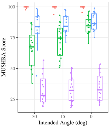</details> REF DSC NO LC DSC LC ANCH Fig. 7: Loudness test: MUSHRA score as a function of the four intended angles [30 ◦ (i), 15 ◦ (ii), 0 ◦ (iii)] and the test condition (REF, DSC NO LC, DSC LC, ANCH). Dots represent the result of each one of the participants, averaged over all 5 content items, and box plots show the corresponding median values and interquartile range. Refer to Fig. 6 for a depiction of the perceived angle deltas with respect to the reference and the results of the paired t -tests. At 30 ◦ (hard panning to the left loudspeaker), all panning methods were statistically indistinguishable from one another ( p ≥ . 4). For the remaining phantom source positions, the average FRC results exhibited a consistent displacement of 9 to 11 degrees towards the closest loudspeaker, with these differences being significant in all cases ( p ≤ 1 × 10 -4 ). The average DSC results were much closer to the reference, but still displayed a slight displacement towards the closest loudspeaker: 6 ◦ (ii), 3 ◦ (iii), and 1 ◦ (iv). The differences were significant in cases (ii) and (iii) ( p ≤ . 002), but not in case (iv) ( p = . 2). 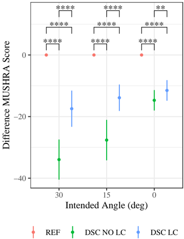Fig. 8: Loudness test: Differential mean MUSHRA scores relative to the reference as a function of the three intended angles and the test condition. Dots represent the mean values and bars the confidence intervals of the mean (95% CL). Results shown have undergone a standarization process betweeen the different participants (see main text). See caption of Fig. 6 for the meaning of the significance stars. <details> <summary>Image 8 Details</summary>  ### Visual Description \n ## Chart: MUSHRA Score Difference vs. Intended Angle ### Overview The image presents a chart displaying the difference in MUSHRA scores across different intended angles (30, 15, and 0 degrees) for three conditions: REF, DSC NO LC, and DSC LC. Error bars are present, and statistical significance is indicated by brackets with asterisks. The chart is a point plot with error bars representing the standard error or confidence interval. ### Components/Axes * **X-axis:** "Intended Angle (deg)" with markers at 30, 15, and 0. * **Y-axis:** "Difference MUSHRA Score" ranging from approximately -50 to 5. * **Legend:** Located at the bottom-center of the chart. * REF (Red): Represented by a salmon-colored point with error bar. * DSC NO LC (Green): Represented by a green point with error bar. * DSC LC (Blue): Represented by a blue point with error bar. * **Statistical Significance Brackets:** Brackets with asterisks (****) are placed above the data points, indicating statistically significant differences between the conditions. The number of asterisks indicates the p-value. ### Detailed Analysis The chart shows the difference in MUSHRA scores for each condition at each intended angle. * **30 Degrees:** * REF: Approximately +2.5, with an error bar extending from approximately 0 to 5. * DSC NO LC: Approximately -35, with an error bar extending from approximately -40 to -30. * DSC LC: Approximately -20, with an error bar extending from approximately -25 to -15. * Statistical significance: REF vs DSC NO LC (****), REF vs DSC LC (****), DSC NO LC vs DSC LC (****). * **15 Degrees:** * REF: Approximately +1, with an error bar extending from approximately -2 to 4. * DSC NO LC: Approximately -25, with an error bar extending from approximately -30 to -20. * DSC LC: Approximately -15, with an error bar extending from approximately -20 to -10. * Statistical significance: REF vs DSC NO LC (****), REF vs DSC LC (****), DSC NO LC vs DSC LC (****). * **0 Degrees:** * REF: Approximately +1, with an error bar extending from approximately -2 to 4. * DSC NO LC: Approximately -20, with an error bar extending from approximately -25 to -15. * DSC LC: Approximately -10, with an error bar extending from approximately -15 to -5. * Statistical significance: REF vs DSC NO LC (****), REF vs DSC LC (*), DSC NO LC vs DSC LC (****). The error bars are roughly the same length for each condition at each angle, suggesting similar variability. ### Key Observations * The REF condition consistently shows a small positive difference in MUSHRA score across all angles. * Both DSC NO LC and DSC LC conditions show negative differences in MUSHRA score, indicating a reduction in quality compared to the REF condition. * DSC NO LC consistently has the lowest MUSHRA score difference, indicating the largest reduction in quality. * The differences between REF and both DSC conditions are statistically significant at all angles. * The difference between DSC NO LC and DSC LC is also statistically significant at all angles. ### Interpretation The data suggests that both DSC NO LC and DSC LC processing methods result in a perceived reduction in quality compared to the REF condition, as measured by the MUSHRA score. DSC NO LC has a more substantial negative impact on perceived quality than DSC LC. The statistical significance of the differences indicates that these effects are not due to random chance. The intended angle appears to have a minor effect on the magnitude of the difference, but the relative ranking of the conditions remains consistent across all angles. The consistent negative differences for DSC conditions suggest a systematic issue with these processing methods, potentially related to artifacts or distortions introduced during the processing. The brackets with asterisks indicate that the differences are statistically significant, meaning they are unlikely to have occurred by chance. The chart demonstrates the impact of different processing methods on perceived visual quality, highlighting the importance of careful processing to maintain high fidelity. </details> ## 5.2 Loudness test Initially we examined whether the test results of the loudness validation test were dependent on the test content. A 3-way repeated measures ANOVA revealed no significant interaction between the test condition and the content item [ F ( 4 . 4 , 38 ) = 2 . 3, p = . 07]. Subsequently, results were averaged over the different source content items. The resulting data distribution is shown in Fig. 7, as a function of the four test conditions (REF, DSC NO LC, DSC LC, ANCH) and the three panning angles [30 ◦ (i), 15 ◦ (ii), 0 ◦ (iii)]. The DSC LC condition always scores in the excellent range (above 80 MUSHRA points). The DSC NO LC condition scores systematically below DSC LC, the difference being greater for panning angles closer to the left loudspeaker. The QQ plot initially indicated moderate deviations from normality, which were determined to be a result of participants rating content on differing scales. To address this, a data normalization procedure was implemented. Specifically, each participant's result was standardized to have zero mean and unit variance. The MUSHRA scale was then restored by multiplying the standarized results by the global variance and adding the global mean. Following this procedure, the QQ plot no longer indicated evident deviations from normality of the data. The anchor was discarded from the subsequent analysis. We conducted a 2-way repeated measures ANOVA to examine the effects of test condition and the intended angle on the results. The ANOVA analysis confirmed a significant main effect for the test condition [ F ( 1 . 4 , 20 . 8 ) = 90 . 3, p = 6 × 10 -10 ] and significant interaction between test condition and intended angle [ F ( 2 . 7 , 40 . 0 ) = 28 . 1, p = 2 × 10 -9 ]. A subsequent post-hoc analysis was conducted, in the form of multiple paired t -tests between the different test conditions (see Fig. 8). Again, Benjamini-Hochberg correction for multiple comparisons [16] was applied. Analysis showed that without loudness correction, scores are on average 33 (i), 27 (ii), and 14 (iii) MUSHRA points lower than the reference on average. With loudness correction, this difference is reduced to 16 (i), 13 (ii), and 12 (iii) MUSHRA points. All mutual comparisons are significant ( p ≤ . 005). ## 6 Discussion The results of the experimental tests show that the common practice to time and level align loudspeakers is insufficient when dealing with non-equidistant loudspeakers, as the phantom source for the FRC system is consistently skewed towards a closer loudspeaker. The average perceived angle delta of about 10 ◦ across all angles under test is high and would result in a significantly impaired playback performance. In all tested cases, using the proposed DSC approach significantly improves the delta angle towards the intended panning position. It is noteworthy that, according to the experiment, DSC performs particularly well in the area in front of the listener, where the human hearing is most sensitive to angular changes. It is worth mentioning that at the largest examined panning angle (15 ◦ ) the experiment still showed a relatively high bias towards the closer loudspeaker (6 ◦ ). While it is possible that the calculated compensation gain was not totally accurate, it could be conceivable that visual cues of the close loudspeaker pull the rating towards it as the intended panning position comes close to it. After all, phantom source localization is a complicated task affected by multi-sensory factors. The results of the loudness validation test are in agreement with our hypothesis that the loudness of phantom sources is not defined by the direct sound, but by the full loudspeaker and room response. Across all tested angles, the DSC panning that was loudness compensated according to the full response, got a mean rating in the excellent range of the MUSHRA scale, in all cases significantly better than the non-loudness compensated version of DSC. The dependence on angle of the ratings for the non-loudness compensated condition nicely match the calculated diminishing dB value as the phantom source is panned further and further away from the closer loudspeaker. It is unsurprising that listeners rated differences between the loudness compensated DSC and the reference system. Those can mainly be attributed to other differences in the systems' characteristics such as direct-to-reverberant ratio or spatial characteristics of close loudspeakers which might not have been fully ignored by the listeners, though instructed to do so. While the formal listening test considered a single phantom source on a stereo layout, typical multimedia content contains many panned objects and the restoring effect to the intended positions using DSC accumulates. Listeners participating in informal listening using a DSC enabled object renderer and multiple loudspeakers reported not only on the restoration of the overall balance, which is otherwise heavily skewed towards close loudspeakers, but also commented on the vastly improved clarity of the mix. These effects were reported to positively affect the rendering, even when the difference in loudspeaker distance was not as substantial as in the presented listening test. Especially in the context of object-based audio and flexible rendering engines at playback time, this approach is a notable step forward towards a faithful representation of the artistic intent in the consumer environment. As object based content makes its way into more and more playback systems like living rooms or cars, the typical loudspeaker setup will be increasingly in-homogeneous and non-equidistant. Instead of forcing consumers to place loudspeakers in canonical positions, the system should be able to adapt. In this paper we have layed out that, as a consequence of the precedence effect, any panning algorithm and renderer will benefit from taking into account the importance of the relative direct sound. ## References - [1] Rumsey, F., Spatial audio , Taylor & Francis, 2012. - [2] Pulkki, V., 'Virtual Sound Source Positioning Using Vector Base Amplitude Panning,' Journal of Audio Engineering Society , 45(6), pp. 456-466, 1997. - [3] Thomas, M. R. and Robinson, C. Q., 'Amplitude panning and the interior pan,' in Audio Engineering Society Convention 143 , 2017. - [4] Lossius, T., Baltazar, P., and de la Hogue, T., 'DBAP - Distance-Based Amplitude Panning,' in International Conference on Mathematics and Computing , 2009. - [5] Tsingos, N., 'Object-Based Audio,' in A. Roginska and P. Geluso, editors, Immersive Sound , pp. 244-275, Routledge, 2017. - [6] Gardner, M. B., 'Historical Background of the Haas and/or Precedence Effect,' The Journal of the Acoustical Society of America , 43(6), pp. 1243-1248, 2005, ISSN 0001-4966. - [7] Haas, H., 'Über den Einflu b eines Einfachechos auf die Hörsamkeit von Sprache,' Acta Acustica united with Acustica , 1(2), pp. 49-58, 1951. - [8] Blauert, J. and Braasch, J., 'Acoustic Communication: The Precedence Effect,' Forum Acusticum Budapest 2005: 4th European Congress on Acustics , 2005. - [9] Blauert, J., Spatial Hearing: The Psychophysics of Human Sound Localization , The MIT Press, 1996. - [10] Bank, B., 'Combined quasi-anechoic and in-room equalization of loudspeaker responses,' in Audio Engineering Society Convention 134 , 2013. - [11] Cecchi, S., Romoli, L., Piazza, F., Bank, B., and Carini, A., 'A novel approach for prototype extraction in a multipoint equalization procedure,' in Audio Engineering Society Convention 136 , 2014. - [12] Matthews, E. A., Simulation and testing of a multichannel system for 3D sound localization , Master's thesis, Graduate School of Western Carolina University, 2015. - [13] Karjalainen, M. and Paatero, T., 'Frequencydependent signal windowing,' in Proceedings of the 2001 IEEE Workshop on the Applications of Signal Processing to Audio and Acoustics , pp. 35-38, 2001. - [14] Schoeffler, M., Bartoschek, S., Stöter, F.-R., Roess, M., Westphal, S., Edler, B., and Herre, J., 'webMUSHRA - A Comprehensive Framework for Web-based Listening Tests,' Journal of Open Research Software , 6, 2018. - [15] Berendes, H.-U., Travaglini, A., and Uhle, C., 'Validating Loudness Alignment Via Subjective Preference: Towards Improving ITU-R BS.17704,' Journal of the Audio Engineering Society , 2022. - [16] ITU-R BS.1534-3, 'Method for the subjective assessment of intermediate quality level of audio systems,' ITU recommendation, 2015. - [17] Kassambara, A., rstatix: Pipe-Friendly Framework for Basic Statistical Tests , 2023, R package version 0.7.2. - [18] R Core Team, R: A Language and Environment for Statistical Computing , Vienna, Austria, 2023.