2311.06788v2

# Real-Time Probabilistic Programming **Authors**: Lars Hummelgren, Matthias Becker, and David Broman > EECS and Digital Futures, KTH Royal Institute of Technology, Sweden {larshum, mabecker, ## Abstract Complex cyber-physical systems interact in real-time and must consider both timing and uncertainty. Developing software for such systems is expensive and difficult, especially when modeling, inference, and real-time behavior must be developed from scratch. Recently, a new kind of language has emerged—called probabilistic programming languages (PPLs)—that simplify modeling and inference by separating the concerns between probabilistic modeling and inference algorithm implementation. However, these languages have primarily been designed for offline problems, not online real-time systems. In this paper, we combine PPLs and real-time programming primitives by introducing the concept of real-time probabilistic programming languages (RTPPL). We develop an RTPPL called ProbTime and demonstrate its usability on an automotive testbed performing indoor positioning and braking. Moreover, we study fundamental properties and design alternatives for runtime behavior, including a new fairness-guided approach that automatically optimizes the accuracy of a ProbTime system under schedulability constraints. ## I Introduction Probabilistic programming [1, 2] is an emerging programming paradigm that enables simple and expressive probabilistic modeling of complex systems. Specifically, the key motivation for probabilistic programming languages (PPLs) is to separate the concerns between the model (the probabilistic program) and the inference algorithm. Such separation enables the system designer to focus on the modeling problem without the need to have deep knowledge of Bayesian inference algorithms, such as Sequential Monte Carlo (SMC) [3, 4] or Markov chain Monte Carlo (MCMC) [5] methods. There are many research PPLs, including Pyro [6], WebPPL [7], Stan [8], Anglican [9], Turing [10], Gen [11], and Miking CorePPL [12]. These PPLs focus on offline inference problems, such as data cleaning [13], phylogenetics [14], computer vision [15], or cognitive science [16], where time and timing properties are not explicitly part of the programming model. Likewise, many languages and environments exist for programming real-time systems [17, 18, 19] with no built-in support for probabilistic modeling and inference. Although some recent work exists on using probabilistic programming for reactive synchronous systems [20, 21] and for continuous time systems [22], no existing work combines probabilistic programming with real-time programming, where both inference and timing constructs are first-class. Combining probabilistic programming with real-time programming results in several significant research challenges. Specifically, we identify two key challenges: (i) how to incorporate language constructs for both timing and probabilistic reasoning in a sound manner, and (ii) how to fairly distribute resources among systems of tasks while considering real-time constraints and inference accuracy requirements. In this paper, we introduce a new kind of language that we call real-time probabilistic programming languages (RTPPLs). In this paradigm, users can focus on the modeling aspect of inferring unknown parameters of the application’s problem space without knowing details of how timing aspects or inference algorithms are implemented. We motivate the ideas behind this new kind of language and outline the main design challenges. To demonstrate the concepts of RTPPL, we develop an RTPPL called ProbTime, which includes probabilistic programming primitives, timing primitives, and primitives for designing modular task-based real-time systems. We create a compiler toolchain for ProbTime and demonstrate how it can be efficiently implemented in an automotive positioning and braking case study. A key aspect of our design is real-time inference using Sequential Monte-Carlo (SMC) and the automatic configuration built on top of this. We have implemented the compiler within the Miking framework [23] as part of the Miking CorePPL effort [12]. ⬇ 2 let x = assume (Beta 2.0 2.0) in \ label {lst: ppl - code: assume} 3 observe true (Bernoulli x); \ label {lst: ppl - code: observe} 4 ...\ label {lst: ppl - code: dots} 5 x \ label {lst: ppl - code: result} (a) Line LABEL:lst:ppl-code:assume defines the latent variable x and gives the prior Beta(2,2). Line LABEL:lst:ppl-code:observe shows an observation statement (observing a true value), and line LABEL:lst:ppl-code:result states that the posterior for x should be computed. <details> <summary>x1.png Details</summary>  ### Visual Description ## [Bar Chart]: Distribution of Values ### Overview The image displays a vertical bar chart (histogram) showing a symmetric, unimodal distribution of values. The chart consists of 21 blue bars of varying heights arranged along an unlabeled horizontal axis. The vertical axis is labeled with numerical values ranging from 0.00 to 0.08. ### Components/Axes * **Vertical Axis (Y-axis):** * **Label:** None explicitly stated. * **Scale:** Linear scale from 0.00 to 0.08. * **Tick Marks & Values:** Major tick marks are present at intervals of 0.01, labeled as: `0.00`, `0.01`, `0.02`, `0.03`, `0.04`, `0.05`, `0.06`, `0.07`, `0.08`. * **Horizontal Axis (X-axis):** * **Label:** None present. * **Categories:** 21 distinct, evenly spaced bars. No category labels or numerical markers are provided. * **Legend:** Not present. * **Chart Title:** Not present. * **Bar Color:** Uniform medium blue for all bars. ### Detailed Analysis The chart displays a clear, symmetric distribution pattern. The bars increase in height from the left, peak in the center, and then decrease symmetrically to the right. **Trend Verification:** The visual trend is a smooth, bell-shaped curve. Starting from the leftmost bar, heights increase steadily, reach a maximum at the two central bars, and then decrease in a mirror-image fashion. **Estimated Bar Heights (from left to right, approximate values based on Y-axis):** 1. ~0.009 2. ~0.022 3. ~0.035 4. ~0.043 5. ~0.053 6. ~0.059 7. ~0.065 8. ~0.069 9. ~0.074 10. **~0.076** (Peak, tied) 11. **~0.076** (Peak, tied) 12. ~0.070 13. ~0.070 14. ~0.065 15. ~0.058 16. ~0.052 17. ~0.044 18. ~0.033 19. ~0.021 20. ~0.008 ### Key Observations 1. **Symmetry:** The distribution is highly symmetric around the central two bars (bars 10 and 11). 2. **Unimodal Peak:** The distribution has a single peak (mode) represented by the two tallest, equal-height bars in the center. 3. **Range:** The values span from approximately 0.008 at the extremes to a peak of approximately 0.076. 4. **Shape:** The overall shape closely resembles a normal (Gaussian) distribution or a binomial distribution. 5. **Missing Context:** The chart lacks a title, axis labels, and a legend, making it impossible to determine what specific data or categories are being represented. ### Interpretation This chart visually demonstrates a fundamental statistical pattern where data points are most frequently clustered around a central value, with frequency tapering off symmetrically towards higher and lower values. * **What it suggests:** The data likely represents a frequency distribution, probability density, or a similar metric where the central tendency is dominant. The perfect symmetry suggests an idealized or theoretical distribution rather than raw, noisy empirical data. * **Relationship of Elements:** The height of each bar is directly proportional to the value on the Y-axis for its corresponding (but unlabeled) category on the X-axis. The arrangement creates a visual representation of concentration and dispersion. * **Notable Patterns:** The most significant pattern is the perfect symmetry and the plateau at the peak (two bars of equal maximum height). This is characteristic of many natural and mathematical phenomena. The absence of any skew or outliers reinforces the impression of a controlled or modeled dataset. * **Underlying Meaning:** Without axis labels, the specific meaning is abstract. However, the form itself is a powerful archetype in data science, representing concepts like the central limit theorem, measurement errors, or the distribution of traits in a population. It communicates balance, predictability, and the prevalence of average values over extremes. 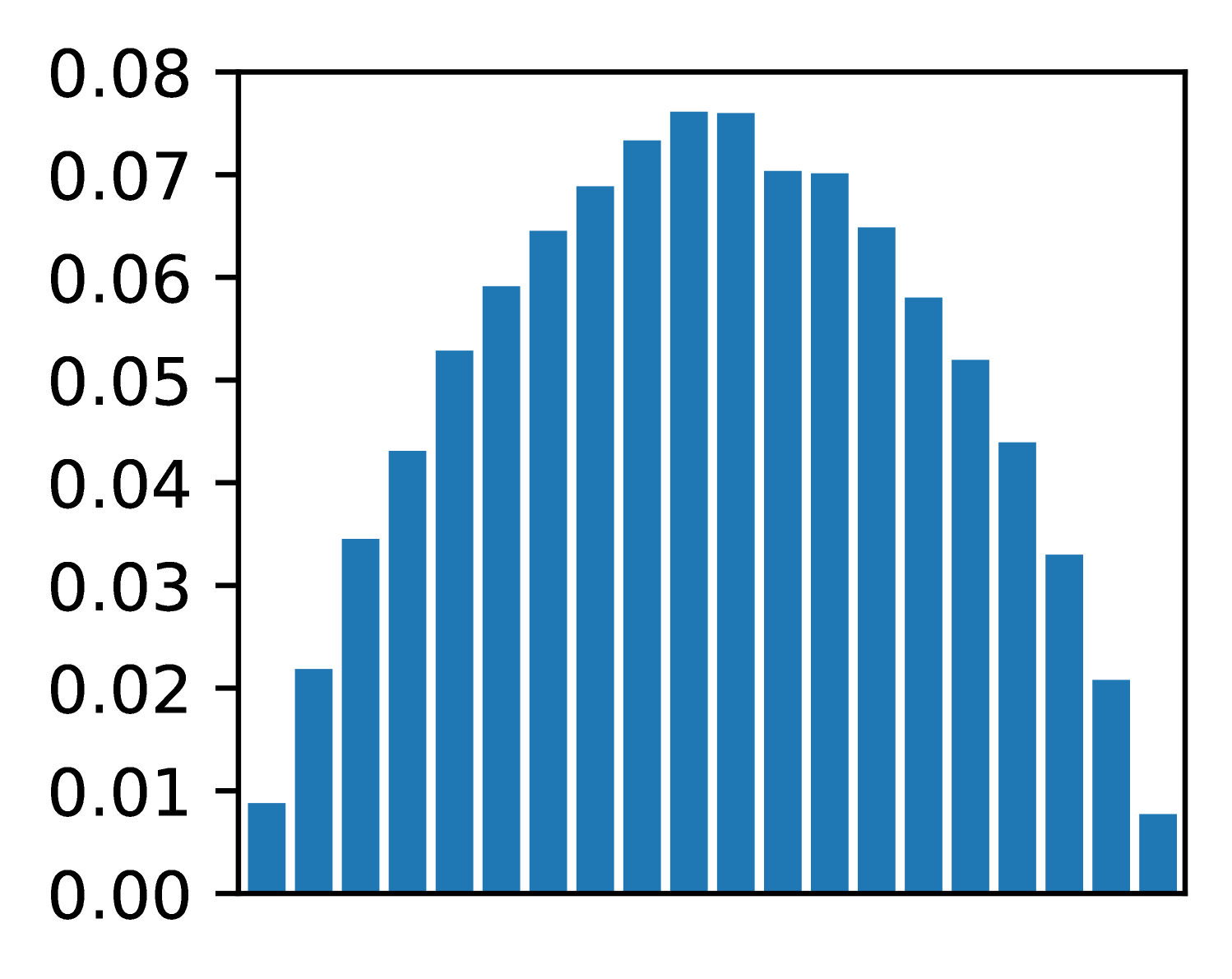</details> (b) Prior distribution Beta(2,2) for latent variable x. <details> <summary>x2.png Details</summary>  ### Visual Description ## Bar Chart: Unlabeled Distribution ### Overview The image displays a vertical bar chart (histogram) showing a unimodal, approximately symmetric distribution of values. The chart consists of 20 blue bars of varying heights plotted against a numerical y-axis. There is no chart title, x-axis label, or legend present. ### Components/Axes * **Y-Axis:** The vertical axis is labeled with numerical values ranging from `0.00` to `0.09` in increments of `0.01`. The axis line and tick marks are clearly visible on the left side of the chart. * **X-Axis:** The horizontal axis is present but has **no labels, title, or tick marks**. It serves only as a baseline for the bars. * **Bars:** There are 20 vertical bars, all of the same solid blue color. They are evenly spaced along the x-axis. * **Legend:** There is **no legend** in the image. * **Title:** There is **no title** for the chart. ### Detailed Analysis The chart depicts a distribution that rises to a central peak and then falls. The trend is as follows: 1. **Ascending Phase:** Starting from the left, the bar heights increase steadily. 2. **Peak:** The distribution reaches its maximum height near the center. 3. **Descending Phase:** After the peak, the bar heights decrease in a roughly mirror-image fashion to the ascent. **Approximate Bar Heights (from left to right):** The following table lists the approximate value for each bar, estimated by aligning the top of the bar with the y-axis scale. Uncertainty is ±0.002. | Bar Position (Left to Right) | Approximate Y-Value | | :--------------------------- | :------------------ | | 1 | 0.000 | | 2 | 0.003 | | 3 | 0.009 | | 4 | 0.016 | | 5 | 0.024 | | 6 | 0.033 | | 7 | 0.042 | | 8 | 0.053 | | 9 | 0.061 | | 10 | 0.071 | | 11 | 0.080 | | 12 | 0.084 | | 13 | 0.086 | | 14 | **0.089 (Peak)** | | 15 | 0.085 | | 16 | 0.079 | | 17 | 0.070 | | 18 | 0.058 | | 19 | 0.039 | | 20 | 0.018 | ### Key Observations * **Distribution Shape:** The data forms a classic bell-shaped or normal-like distribution. * **Symmetry:** The distribution is roughly symmetric around the 14th bar (the peak). * **Peak Location:** The highest frequency (tallest bar) is the 14th bar from the left, with a value of approximately `0.089`. * **Range:** The values span from near `0.00` to just below `0.09`. * **Missing Context:** The complete absence of an x-axis label or chart title makes it impossible to determine what variable is being measured or what the categories/bins represent. ### Interpretation This chart visually demonstrates a dataset where the majority of observations cluster around a central value, with fewer observations at the extremes. The shape is characteristic of many natural and statistical phenomena (e.g., measurement errors, heights of a population). The **key investigative insight** is the profound lack of context. While the *pattern* of the data is clear, its *meaning* is entirely obscured. The chart shows *that* there is a distribution, but not *what* is distributed. To make this data useful, critical metadata is required: the title of the chart, the label for the x-axis (defining the bins or categories), and the unit of measurement for the y-axis (e.g., probability density, frequency, count). Without this information, the chart is an abstract representation of a distribution pattern only. 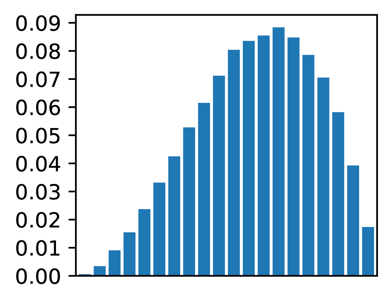</details> (c) Posterior distribution for x, one true observation. <details> <summary>x3.png Details</summary>  ### Visual Description ## Histogram: Unlabeled Distribution ### Overview The image displays a vertical bar chart (histogram) showing a symmetric, unimodal distribution of data. The chart consists of 21 blue bars of varying heights arranged along an unlabeled horizontal axis. The vertical axis represents a numerical scale, likely frequency, probability density, or proportion. ### Components/Axes * **Vertical Axis (Y-axis):** * **Label:** None visible. * **Scale:** Linear scale ranging from 0.00 to 0.12. * **Tick Marks & Values:** Major tick marks are present at intervals of 0.01, with numerical labels for every tick: 0.00, 0.01, 0.02, 0.03, 0.04, 0.05, 0.06, 0.07, 0.08, 0.09, 0.10, 0.11, 0.12. * **Horizontal Axis (X-axis):** * **Label:** None visible. * **Scale:** Unlabeled categorical or binned numerical scale. The axis is divided into 21 discrete positions, each occupied by a single bar. * **Data Series:** * **Color:** All bars are a uniform shade of blue. * **Legend:** No legend is present. * **Spatial Layout:** The chart is contained within a black rectangular border. The y-axis labels are positioned to the left of the axis line. The bars are centered on their respective x-axis positions. ### Detailed Analysis The distribution is symmetric and bell-shaped, peaking at the center. Below are the approximate heights of each bar, listed from left to right. Values are estimated based on visual alignment with the y-axis grid. 1. Bar 1 (far left): ~0.002 2. Bar 2: ~0.008 3. Bar 3: ~0.017 4. Bar 4: ~0.032 5. Bar 5: ~0.048 6. Bar 6: ~0.068 7. Bar 7: ~0.085 8. Bar 8: ~0.103 9. Bar 9: ~0.113 10. **Bar 10 (Center, Peak): ~0.118** 11. Bar 11: ~0.113 12. Bar 12: ~0.100 13. Bar 13: ~0.084 14. Bar 14: ~0.059 15. Bar 15: ~0.035 16. Bar 16: ~0.017 17. Bar 17: ~0.005 18. Bars 18-21: Heights are very low, tapering to near zero. (Bar 18: ~0.003, Bar 19: ~0.001, Bars 20 & 21: ~0.000). **Trend Verification:** The data series forms a clear, symmetric peak. The trend slopes upward from the left, reaches a maximum at the 10th bar, and then slopes downward symmetrically to the right. ### Key Observations 1. **Symmetry:** The distribution is highly symmetric around the central (10th) bar. 2. **Unimodal:** There is a single, clear peak. 3. **Peak Value:** The maximum value is approximately 0.118, located at the center of the distribution. 4. **Range:** The data spans from near 0.000 at the extremes to ~0.118 at the peak. 5. **Missing Context:** The complete absence of labels for both axes and any title or legend makes it impossible to determine what the data represents (e.g., test scores, measurement errors, signal strength). ### Interpretation The chart visually demonstrates a classic **normal (Gaussian) distribution** or a very close approximation. The data suggests that the measured variable is most frequently found near the central value, with frequencies decreasing symmetrically as one moves away from the center in either direction. The **key investigative insight** is the profound lack of context. While the *shape* of the data is clear and informative (indicating a process governed by random variation or central tendency), the *meaning* is entirely absent. To make this chart useful, one must answer: What is on the X-axis? (e.g., "Height in cm," "Voltage Deviation"). What is on the Y-axis? (e.g., "Relative Frequency," "Probability Density"). Without this information, the chart is a pure mathematical form without real-world application. The next logical step for an investigator would be to locate the source of this image to obtain the missing metadata. 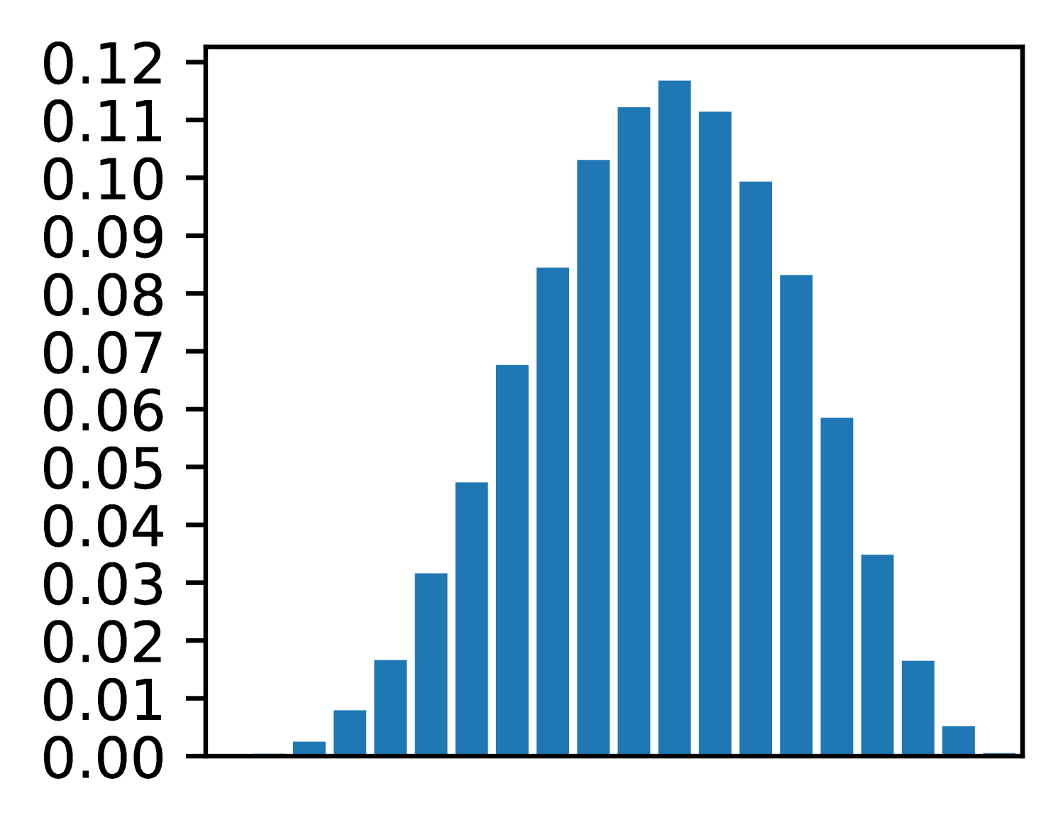</details> (d) Posterior distri-bution, observations [T, F, F, T, T] Figure 1: A simple CorePPL program modeling a coin flip. Fig. (1(a)) shows the source code, and Fig. (1(b)) the prior distribution. Fig. (1(c)) gives the posterior distribution after one coin flip, and Fig. (1(d)) the posterior after a sequence of 5 coin flips. In summary, we make the following contributions: - We introduce the new paradigm of real-time probabilistic programming languages (RTPPL), motivate why it is essential, and outline significant design challenges (Sec. II). - We design and implement ProbTime, a language within the domain of RTPPL (Sec. III), and specify its formal behavior (Sec. IV). - We present a novel automated offline configuration approach that maximizes inference accuracy under timing constraints. Specifically, we introduce the concepts of execution-time and particle fairness within the context of real-time probabilistic programming (Sec. V) and study how they can be incorporated in an automated configuration setting (Sec. VI). - We develop an automotive testbed including both hardware and software. As part of our case study, we demonstrate how a non-trivial ProbTime program can perform indoor positioning and braking in a real-time physical environment (Sec. VII). ## II Motivation and Challenges with RTPPL This section introduces the main ideas of probabilistic programming, motivates why it is useful for real-time systems, and outlines some of the key challenges. ### II-A Probabilistic Programming Languages (PPLs) Probabilistic programming is a rather recent programming paradigm that enables probabilistic modeling where the models can be described as Turing complete programs. Specifically, given a probabilistic program $f$ , observed data, and prior knowledge about the distribution of latent variables $\theta$ , a PPL execution environment can automatically approximate the posterior distribution of $\theta$ . Recall Bayes’ rule $$ \displaystyle p(\theta,\textbf{data})=\frac{p(\textbf{data},\theta)p(\theta)}{ p(\textbf{data})} \tag{1} $$ where $p(\theta,\textbf{data})$ is the posterior, $p(\textbf{data},\theta)$ the likelihood, $p(\theta)$ the prior, and $p(\textbf{data})$ the normalizing constant. Using a simple toy probabilistic program, we explain how standard PPL constructs relate to Bayes’ rule. Consider Fig. 1(a), written in CorePPL [12], the core language that our work is based on. We use this coin-flip example to give an intuition of the fundamental constructs in a PPL. The model starts by defining a random variable x (line LABEL:lst:ppl-code:assume) using the assume construct. In this example, random variable x models the probability that a coin flip becomes true (we let true mean heads and false mean tails). For instance, if $p(\texttt{x})=0.5$ , the coin is fair, whereas if, e.g., $p(\texttt{x})=0.7$ , it is unfair and more likely to result in true when flipped. The assume construct on line LABEL:lst:ppl-code:assume defines the random variable and gives its prior; in this case, the Beta distribution with both parameters equal to $2$ . If we sample from this prior, we get the Beta distribution depicted in Fig. 1(b). Note how the sample constructs in a probabilistic program (assume in CorePPL) correspond to the prior $p(\theta)$ in Bayes’ rule (Equation 1). However, the goal of Bayesian inference is to estimate the posterior for a latent variable, given some observations. Line LABEL:lst:ppl-code:observe in the program shows an observe statement, where a coin flip of value true is observed according to the Bernoulli distribution. Note how the Bernoulli distribution’s parameter depends on the random variable x. Consider Fig. 1(c), which depicts the inferred posterior distribution given one observed true coin flip. As expected, the distribution shifts slightly to the right, meaning that given one sample, the coin is estimated to be somewhat biased toward true. Note also how observe statements in a probabilistic program correspond to the likelihood $p(\textbf{data},\theta)$ in Bayes’ rule. That is, the likelihood we observe specific data, given a certain latent variable $\theta$ . If we extend Fig. 1(a) with in total five observations [true, false, false, true, true] in a sequence (illustrated with ... on line LABEL:lst:ppl-code:dots), the resulting posterior looks like Fig. 1(d). We can note the following: (i) the resulting mean is still slightly biased toward true (we have observed one more true value), and (ii) the variance is lower (the peak is slightly thinner). The latter case is a direct consequence of Bayesian inference and one of its key benefits: given the prior and the observed data, the posterior correctly represents the uncertainty of the result, not just a point estimate. There are many inference strategies that can be used for the inference in the toy example, such as sequential Monte Carlo (SMC) or Markov chain Monte Carlo (MCMC). In this work, we focus on SMC and one of its instances, also known as the particle filter [24] algorithm, because of its strength in this kind of application. The intuition of particle filters is that inference is done by executing the probabilistic program (the model) multiple times (potentially in parallel). Each such execution point is called a particle and consists at the end of a weight (how likely the particle is) and the output values, where the set of all particles forms the posterior distribution. Intuitively, the more particles, the better the accuracy of the approximate inference. Many more details of the algorithm (e.g., resampling strategies) are outside this paper’s scope, and an interested reader is referred to this technical overview by Naesseth et al. [25]. Although hiding the details of the inference algorithm is one of the key ideas of PPLs (separating the model from inference), the number of particles is essential for automatic inference and scheduling. Hence, this is a key concept in our work and will be discussed further in this paper. ### II-B Real-Time Probabilistic Programming (RTPPL) ⬇ 46 system { 47 sensor speed1 : Float rate 50 ms ///\label{lst:model:sa1} 48 sensor speed2 : Float rate 100 ms 49 actuator brake : Float rate 500 ms ///\label{lst:model:sa2} 50 task speedEst1 = Speed (250 ms) importance 1 ///\label{lst:model:tasks1} 51 task speedEst2 = Speed (500 ms) importance 1 52 task pos = Position () importance 3 53 task braking = Brake (300 ms) importance 4 ///\label{lst:model:tasks2} 54 speed1 -> speedEst1. in1 ///\label{lst:model:conn1} 55 speed2 -> speedEst2. in1 56 speedEst1. out -> pos. in1 ///\label{lst:model:s1conn1} 57 speedEst1. out -> braking. in1 ///\label{lst:model:s1conn2} 58 speedEst2. out -> pos. in2 59 speedEst2. out -> braking. in2 60 pos. out -> braking. in3 61 braking. out -> brake } ///\label{lst:model:conn2} (a) The system declaration of a ProbTime program. <details> <summary>x4.png Details</summary>  ### Visual Description ## System Block Diagram: Speed Estimation and Braking Control ### Overview The image displays a technical block diagram representing a control system for speed estimation and braking. The diagram illustrates the flow of signals from two speed inputs, through estimation and processing blocks, to a final braking output. It is a functional schematic, not a data chart, so no numerical values or trends are present. The structure suggests a redundant or dual-channel system for safety-critical applications. ### Components/Axes The diagram consists of the following components, connected by labeled signal lines: **Input Sources (Ovals, Left Side):** * `speed1` (Top-left oval) * `speed2` (Bottom-left oval) **Processing Blocks (Rectangles, Center):** * `speedEst1` (Top-center rectangle) * `speedEst2` (Bottom-center rectangle) * `pos` (Top-right rectangle) * `braking` (Bottom-right rectangle) **Output Sink (Oval, Right Side):** * `brake` (Far-right oval) **Signal Connections (Labeled Lines):** * From `speed1` to `speedEst1`: Labeled `in1` * From `speed2` to `speedEst2`: Labeled `in1` * From `speedEst1` to `pos`: Labeled `out` (from speedEst1) to `in1` (of pos) * From `speedEst1` to `braking`: Labeled `out` (from speedEst1) to `in1` (of braking) * From `speedEst2` to `pos`: Labeled `out` (from speedEst2) to `in2` (of pos) * From `speedEst2` to `braking`: Labeled `out` (from speedEst2) to `in2` (of braking) * From `pos` to `braking`: Labeled `out` (from pos) to `in3` (of braking) * From `braking` to `brake`: Labeled `out` ### Detailed Analysis The system architecture is as follows: 1. **Input Stage:** Two independent speed signals (`speed1`, `speed2`) are provided. 2. **Estimation Stage:** Each speed signal is processed by its own dedicated estimator block (`speedEst1`, `speedEst2`). The output of each estimator is a single signal. 3. **Processing & Fusion Stage:** * The `pos` block receives both estimated speed signals (`in1` from `speedEst1`, `in2` from `speedEst2`). Its function is likely to calculate a position or a fused speed/position metric. * The `braking` control block is the central decision unit. It receives three inputs: the two raw estimated speeds (`in1` from `speedEst1`, `in2` from `speedEst2`) and the processed output from the `pos` block (`in3`). 4. **Output Stage:** The `braking` block generates a single control signal (`out`) that is sent to the final actuator or system labeled `brake`. ### Key Observations * **Redundancy:** The system uses two parallel speed estimation channels (`speedEst1` and `speedEst2`), which is a common design pattern for fault tolerance and reliability in safety-critical systems (e.g., automotive, aerospace). * **Signal Routing:** The output of `speedEst1` is routed to two different downstream blocks (`pos` and `braking`). Similarly, the output of `speedEst2` is also routed to both `pos` and `braking`. * **Hierarchical Control:** The `braking` block integrates information from three distinct sources: the two direct speed estimates and a derived metric from the `pos` block. This suggests a sophisticated control algorithm that considers multiple factors before issuing a brake command. * **Unidirectional Flow:** All signal arrows point from left to right, indicating a feed-forward control system with no visible feedback loops in this diagram. ### Interpretation This block diagram represents the logical architecture of a **dual-redundant speed-sensing and braking control system**. The primary purpose is to generate a reliable `brake` command based on multiple, independently derived speed measurements. * **What it demonstrates:** The system prioritizes reliability and fault detection. By having two separate speed estimators, the system can potentially cross-check their outputs. If one estimator fails or provides erroneous data, the `braking` logic (which also receives the `pos` signal) can still make a safe decision. The inclusion of a `pos` block suggests the braking decision is not based on speed alone but also on positional or derived kinematic data. * **Relationships:** The `pos` block acts as a data fusion point for the two speed estimates, while the `braking` block acts as the final decision-making controller, fusing all available information. The `brake` oval is the actuator or system being controlled. * **Potential Application:** This architecture is characteristic of systems where failure is not an option, such as in advanced driver-assistance systems (ADAS), autonomous vehicles, industrial machinery, or railway signaling. The diagram itself is a high-level functional view; the actual implementation within each block (e.g., the algorithms inside `speedEst1` or `braking`) is not specified. 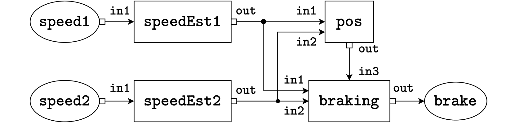</details> (b) A graphical representation of the system defined in Fig. 2(a). The system consists of two sensors, speed1 and speed2 on the left-hand side, four tasks speedEst1, speedEst2, pos, and braking in the middle, and an actuator brake on the right-hand side. Lines represent connections, where the white box represents the output port and the incoming arrow represents the input port. Figure 2: Example system of a ProbTime program in textual (2(a)) and graphical form (2(b)). The toy example of a coin flip in the previous example gives an intuition of probabilistic programming but does not show its power in large-scale applications. Probabilistic programming is used in several domains today, but surprisingly, little has been done in the context of time-critical applications. Although a rich literature exists on using Bayesian inference and filtering algorithms (e.g., particle filters in aircraft positioning [24]), these algorithms are typically hand-coded where both the probabilistic model and the inference algorithm are combined. This means that a developer needs to have deep insights into three different fields: (i) probabilistic modeling, (ii) Bayesian inference algorithms, and (iii) real-time programming aspects. Standard probabilistic programming is motivated by the appealing argument of separating (i) and (ii), thus enabling probabilistic modeling by developers without deep knowledge of how to implement inference efficiently and correctly. However, so far, probabilistic programming has not been combined with (iii) real-time aspects, such as timing, scheduling, and worst-case execution time estimation. This paper aims to make the first step towards mitigating this gap. We call this approach real-time probabilistic programming (RTPPL). How can an RTPPL be designed? For instance, we can extend an existing PPL with timing semantics, extend an existing real-time language with PPL constructs, or create a new domain-specific language (DSL) including only a minimal number of constructs for reasoning about timing and probabilistic inference. In this research work, we choose the latter to avoid complexity when extending large existing languages. In particular, our purpose is to create this rather small research language to study the fundamentals of this new kind of language category. We identify and examine the following key challenges with RTPPLs: - Challenge A: In an RTPPL, how can we encode real-time properties (deadlines, periodicity, etc.) and probabilistic constructs (sampling, observations, etc.) without forcing the user to specify low-level details such as particle counts and worst-case execution times? - Challenge B: How can a runtime environment be constructed, such that a fair amount of time is spent on different tasks, giving the right number of particles for each task (for accuracy), where the system is still known to be statically schedulable? We first address Challenge A (Sec. III - IV) by designing a new minimalistic research DSL called ProbTime and defining its formal behavior. Using the new DSL, we address Challenge B by studying two new concepts: execution-time fairness and particle fairness (Sec. V), and how particle counts, execution-time measurements, and scheduling can be performed automatically to get a fair and working configuration (Sec. VI). ## III ProbTime - an RTPPL In this section, we introduce a new real-time probabilistic programming language called ProbTime. We present the timing and probabilistic constructs in the language using a small example, followed by an overview of the compiler implementation. ProbTime is open-source and publically available https://github.com/miking-lang/ProbTime. ### III-A System Declaration We present a ProbTime system declaration implementing automated braking for a train in Fig. 2. The system keeps track of the train’s position and uses the automatic brakes before reaching the end of the track. The train provides observation data via two speed sensors with varying frequencies and accuracy (left side of Fig. 2(b)), and the system can activate the brakes via an actuator (right side of Fig. 2(b)). In Fig. 2(a), we first declare the sensors and actuators and associate them with a type to indicate what kind of data they operate on (lines LABEL:lst:model:sa1 - LABEL:lst:model:sa2). We also specify the rate at which data is provided by sensors and consumed by actuators. The squares in the graphical representation correspond to the tasks of our system. We instantiate the tasks on lines LABEL:lst:model:tasks1 - LABEL:lst:model:tasks2. Note that speedEst1 and speedEst2 are instantiated from the same template. The importance construct captures the relative importance of tasks. We use the importance value to indicate how important the quality of inference performed by a task is. It is not to be confused with the task priority. As we saw in the coin flip example (Sec. II), the number of particles used in inference relates to the quality of the estimate. In the train example, we use importance on lines LABEL:lst:model:tasks1 - LABEL:lst:model:tasks2 to indicate that pos and braking should run more particles than speedEst1 and speedEst2. We discuss importance in more detail in Sec. V. On lines LABEL:lst:model:conn1 - LABEL:lst:model:conn2 in Fig. 2(a), we declare the connections using arrow syntax a -> b, specifying that data written to output port a is delivered to input port b. Names of sensors and actuators represent ports and x.y refers to port y of task x. ### III-B Templates and Timing Constructs Continuing with the train braking example, we outline the definitions of the task templates Speed and Position in Listing 1. Consider the definition of the Speed template (lines LABEL:lst:model:speed1 - LABEL:lst:model:speed2). We declare the input port in1 and the output port out on lines LABEL:lst:model:speedin1 - LABEL:lst:model:speedout, and annotate them with types. We control timing in ProbTime using the iterative periodic block statement. A periodic block is a loop where each iteration starts after a statically known delay. Each iteration constitutes a task instance. On lines LABEL:lst:model:speed-periodic - LABEL:lst:model:speed2, we define a periodic block whose period is determined by the period argument of the Speed template. For instance, if period is $1\text{\,}\mathrm{s}$ , the release time is one second after the release time of the previous iteration. Our approach to timing is similar to the logical execution time paradigm [26]. However, while all timestamps are absolute under the hood, we only expose a relative view of the logical time of the current task instance. The read statement retrieves a sequence of inputs available from an input port at the logical time of the task instance. On line LABEL:lst:model:speed-read, we retrieve inputs from port in1 and store them in the variable obs. Similarly, the write statement (line LABEL:lst:model:speed-write) sends a message with a given payload to the specified output port. In Position (lines LABEL:lst:model:pos1 - LABEL:lst:model:pos2), we use our prior belief of the train’s position when estimating its current position. However, variables in ProbTime are immutable by default. We use update d in the periodic block on line LABEL:lst:model:pos-upd to indicate that updates to d (the position distribution) should be visible in subsequent iterations. Also, in the write on line LABEL:lst:model:pos-write, we specify an offset to the timestamp of the message relative to the current logical time of the task (it is zero by default). Listing 1: Definition of the Speed and Position task templates. ⬇ 20 template Speed (period : Int) {///\label{lst:model:speed1} 21 input in1 : Float ///\label{lst:model:speedin1} 22 output out : Dist (Float) ///\label{lst:model:speedout} 23 periodic period {///\label{lst:model:speed-periodic} 24 read in1 to obs ///\label{lst:model:speed-read} 25 infer speedModel (obs) to d ///\label{lst:model:speed-infer} 26 write d to out } } ///\label{lst:model:speed-write} \label{lst:model:speed2} 27 template Position () {///\label{lst:model:pos1} 28 input in1 : Dist (Float) 29 input in2 : Dist (Float) 30 output out : Dist (Float) 31 infer initPos () to d 32 periodic 1 s update d {///\label{lst:model:pos-upd} 33 read in1 to speed1 34 read in2 to speed2 35 infer positionModel (d, speed1, speed2) to d 36 write d to out offset 500 ms } } ///\label{lst:model:pos-write} \label{lst:model:pos2} ### III-C Models and Probabilistic Constructs We define three probabilistic constructs in ProbTime, similar to what is used in other PPLs: sample, observe, and infer. We use sample and observe when defining probabilistic models, and we use the infer construct to produce a distribution from a probabilistic model in task templates. Listing 2: Probabilistic model for estimating the train’s speed. ⬇ 10 model speedModel (obs : [TSV (Float)]) : Float {///\label{lst:model:model1} 11 sample b $\sim$ Uniform (0.0, maxSpeed) ///\label{lst:model:intercept} 12 sample m $\sim$ Gaussian (0.0, 1.0) 13 sample sigma $\sim$ Gamma (1.0, 1.0) ///\label{lst:model:sigma} 14 for o in obs {///\label{lst:model:for1} 15 var ts = timestamp (o) ///\label{lst:model:to-timestamp} 16 var x = intToFloat (ts) / intToFloat (1 s) ///\label{lst:model:tstofloat} 17 var y = m * x + b 18 observe value (o) $\sim$ Gaussian (y, sigma) } ///\label{lst:model:observe} \label{lst:model:for2} 19 return b } ///\label{lst:model:model-ret} \label{lst:model:model2} Consider the probabilistic model defined using the function speedModel in Listing 2. The function models the speed of the train at the current logical time using Bayesian linear regression. The parameter obs is a sequence of speed observations encoded as a sequence of floating-point messages (we use TSV as a short-hand for timestamped values). In this model, we use a sample statement to sample a random slope and intercept of a line, assuming acceleration is constant. There are three latent variables (defined on lines LABEL:lst:model:intercept - LABEL:lst:model:sigma): b (the offset of the line), m (the slope of the line), and sigma (the variance, approximating the uncertainty of the estimate). The estimated line can be seen as a function of the speed over (relative) time, where $0 0$ is the logical time of the task instance. 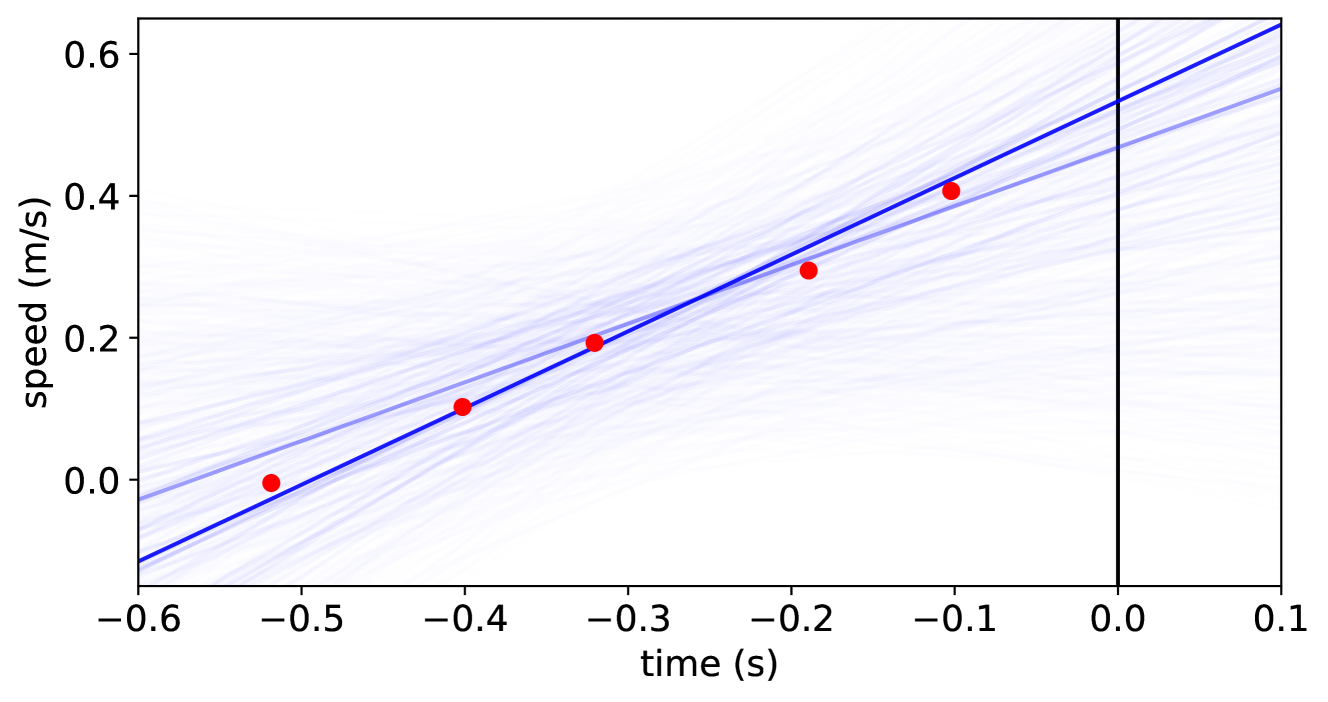In the for-loop on lines LABEL:lst:model:for1 - LABEL:lst:model:for2, we update our belief based on the speed observations. First, we translate the relative timestamp of the observation o to a floating-point number, representing our x-value (lines LABEL:lst:model:to-timestamp - LABEL:lst:model:tstofloat). We use the observe statement on line LABEL:lst:model:observe to update our belief. The observed value is the data of o (retrieved using value(o)), and we expect observations to be distributed according to a Gaussian distribution centered around the y-value. We return the train’s estimated speed (the intercept of the line) on line LABEL:lst:model:model-ret. Figure 3 presents a sample plot of what this looks like when the train accelerates. As we use relative timestamps in ProbTime, we can define this rather complicated model succinctly. <details> <summary>x5.png Details</summary>  ### Visual Description ## Scatter Plot with Trend Line and Confidence Bands: Speed vs. Time ### Overview The image is a scatter plot illustrating the relationship between **time (in seconds)** (x-axis) and **speed (in meters per second)** (y-axis). It includes red data points, a blue linear trend line, light blue confidence bands (or multiple model fits), and a vertical black reference line at \( x = 0 \) (time = 0 s). ### Components/Axes - **X-axis (Horizontal)**: - Label: `time (s)` - Ticks: \(-0.6, -0.5, -0.4, -0.3, -0.2, -0.1, 0.0, 0.1\) (spanning ~\(-0.6\) to \(0.1\) seconds). - **Y-axis (Vertical)**: - Label: `speed (m/s)` - Ticks: \(0.0, 0.2, 0.4, 0.6\) (spanning ~\(-0.1\) to \(0.6\) m/s, as the trend line starts below \(0.0\) at \(x = -0.6\)). - **Data Points (Red Dots)**: Approximate coordinates (time, speed): - \((-0.5, 0.0)\) - \((-0.4, 0.1)\) - \((-0.3, 0.2)\) - \((-0.2, 0.3)\) - \((-0.1, 0.4)\) - **Trend Line (Blue)**: A linear line with a **positive slope** (increasing from left to right), passing through/near the red data points. - **Confidence Bands (Light Blue Lines)**: Multiple light blue lines surrounding the blue trend line, indicating variability/uncertainty in the model (e.g., confidence intervals or multiple model fits). - **Vertical Reference Line (Black)**: At \( x = 0 \) (time = 0 s), likely a critical time point (e.g., event trigger, measurement start). ### Detailed Analysis - **Data Trend**: The red dots show a **strong positive linear relationship** between time and speed. As time increases (moves from \(-0.5\) to \(-0.1\) s), speed increases (from ~\(0.0\) to ~\(0.4\) m/s). The spacing between points is consistent (each ~\(0.1\) s in time, ~\(0.1\) m/s in speed), reinforcing linearity. - **Trend Line Slope**: The blue line has a slope of ~\(1\) m/s² (since speed vs. time slope = acceleration). For example: - From \( x = -0.5 \) (speed = \(0.0\) m/s) to \( x = -0.1 \) (speed = \(0.4\) m/s): \(\Delta \text{time} = 0.4\) s, \(\Delta \text{speed} = 0.4\) m/s → Slope = \(0.4 / 0.4 = 1\) m/s². - **Confidence Bands**: The light blue lines are wider at the extremes (\(x = -0.6\) and \(x = 0.1\)) and narrower in the middle, typical of linear regression confidence intervals (uncertainty increases at the edges of the data range). - **Vertical Line at \( x = 0 \)**: At \( x = 0 \), the blue trend line predicts a speed of ~\(0.5\) m/s (extrapolating from \( x = -0.1 \) (speed = \(0.4\) m/s) to \( x = 0 \)). ### Key Observations - **Linear Consistency**: All red data points lie close to the blue trend line, with no obvious outliers. - **Uniform Spacing**: Data points are evenly spaced in time (~\(0.1\) s intervals) and speed (~\(0.1\) m/s intervals), confirming a linear pattern. - **Confidence Band Symmetry**: Light blue lines are symmetric around the trend line, indicating a well-behaved model with balanced uncertainty. ### Interpretation - **What the Data Suggests**: The plot demonstrates a **constant acceleration** (linear speed-time relationship). The red points, blue trend line, and light blue bands collectively show that speed increases linearly with time, with consistent uncertainty. - **Element Relationships**: Time (x-axis) is the independent variable, speed (y-axis) is the dependent variable. The red points are observed data, the blue line is the best-fit model, and the light blue lines represent uncertainty. The vertical line at \( x = 0 \) likely marks a critical time (e.g., experiment start). - **Trends/Anomalies**: No anomalies; the linear trend is robust across the time range. The confidence bands confirm the model’s reliability, with uncertainty increasing at the data’s edges. This description captures all visual elements, trends, and relationships, enabling reconstruction of the plot’s information without the image. </details> Figure 3: Outcome of the speed model for the speedEst2 task on synthetic data. The x-axis represents time in seconds, and the y-axis represents the train’s speed in meters per second (we seek the speed at the current time, $x=0.0$ ). The red dots represent speed observations, and the blue lines are estimates from the model (slope and intercept), where the opacity of a line indicates its likelihood. <details> <summary>x6.png Details</summary>  ### Visual Description ## Diagram: ProbTime Compilation Pipeline ### Overview The image is a horizontal flowchart illustrating a multi-stage compilation pipeline for a system called "ProbTime." The diagram depicts the transformation of a source program into final executable files through a series of processing stages, represented by blue boxes (active components) and gray boxes (data structures or inputs/outputs). The flow proceeds from left to right, with some components having auxiliary inputs or side processes. ### Components/Axes The diagram is organized as a sequence of processing stages connected by directional arrows. The primary components are: 1. **ProbTime Program** (Gray box, far left): The initial input source code. 2. **Parser** (Blue box, labeled with circled number **1**): The first processing stage. 3. **ProbTime AST** (Gray box): The Abstract Syntax Tree output from the parser. 4. **Validator** (Blue box, labeled with circled number **2**): A component positioned above the "ProbTime AST," connected by an upward arrow, indicating a validation or checking process on the AST. 5. **Extractor** (Blue box, labeled with circled number **3**): The next main processing stage. 6. **ProbTime Runtime** (Gray box, above the Extractor): An input or dependency for the Extractor, connected by a downward arrow. 7. **System Declaration** (Gray box, above and to the right of the Extractor): Another input for the Extractor, connected by a diagonal arrow. 8. **ProbTime Task ASTs** (Stack of gray boxes): The output from the Extractor, representing multiple task-specific Abstract Syntax Trees. 9. **Backend Compiler** (Blue box, labeled with circled number **4**): Processes the Task ASTs. 10. **CorePPL ASTs** (Stack of gray boxes, inside a dashed rectangle): An intermediate representation output from the Backend Compiler. 11. **CorePPL Compiler** (Blue box, labeled with circled number **5**, inside the dashed rectangle): The final compilation stage. 12. **ProbTime Executables** (Stack of gray boxes, top right): The final output of the pipeline, connected by an upward arrow from the CorePPL Compiler. ### Detailed Analysis The pipeline flow is as follows: 1. The **ProbTime Program** is fed into the **Parser (1)**. 2. The Parser produces a **ProbTime AST**. 3. The **Validator (2)** operates on this AST (likely for syntax or semantic checks). 4. The validated AST is passed to the **Extractor (3)**. 5. The Extractor uses two additional inputs: the **ProbTime Runtime** and a **System Declaration**. 6. The Extractor's output is a set of **ProbTime Task ASTs**. 7. These Task ASTs are processed by the **Backend Compiler (4)**. 8. The Backend Compiler generates **CorePPL ASTs** (contained within a dashed boundary, suggesting a specific compilation phase or module). 9. The **CorePPL Compiler (5)** processes these ASTs. 10. The final output is a set of **ProbTime Executables**. ### Key Observations * **Staged Architecture:** The process is clearly divided into discrete, numbered stages (1-5), each represented by a blue box. * **Data Transformation:** Gray boxes represent data structures (ASTs, programs, executables) that are transformed by the blue processing components. * **Parallel Outputs:** The use of stacked boxes for "ProbTime Task ASTs," "CorePPL ASTs," and "ProbTime Executables" indicates that the pipeline can handle multiple tasks or produce multiple outputs in parallel. * **Modular Design:** The dashed rectangle around the CorePPL stages (ASTs and Compiler) suggests this is a distinct subsystem or a reusable compilation backend. * **Auxiliary Inputs:** The Extractor stage is notable for having two external inputs (Runtime and System Declaration), implying it performs context-aware extraction or code generation. ### Interpretation This diagram represents a sophisticated compiler toolchain designed for a probabilistic real-time programming domain ("ProbTime"). The pipeline's structure reveals a clear separation of concerns: * **Frontend (Stages 1-3):** Handles parsing, validation, and extraction of high-level program constructs into task-specific representations, incorporating runtime and system constraints. * **Mid-end (Stage 4):** The Backend Compiler likely performs optimizations or transformations from the domain-specific Task ASTs to a more general intermediate representation (CorePPL ASTs). * **Backend (Stage 5):** The CorePPL Compiler generates the final machine-executable code. The presence of a dedicated "Validator" and the use of "System Declaration" and "ProbTime Runtime" as inputs to the Extractor suggest that correctness, timing guarantees, and adherence to system constraints are critical concerns in this compilation process. The overall flow demonstrates how a high-level probabilistic program is systematically decomposed, validated, and transformed into efficient, runnable executables for a real-time system. 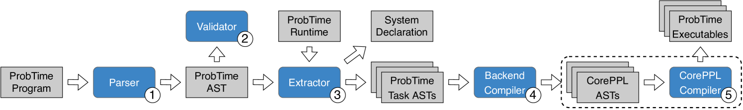</details> Figure 4: An overview of the ProbTime compiler. Gray square boxes represent artifacts, and rounded blue squares represent compiler transformations (numbered by the order in which they run). We use the pre-existing CorePPL compiler to produce executable code in the dashed area. Finally, recall Listing 1 at line LABEL:lst:model:speed-infer, where we use the infer statement to infer the posterior using the probabilistic model (in this case speedModel). ### III-D Compiler Implementation Fig. 4 depicts the key steps of the ProbTime compiler. The compiler is implemented within the Miking framework [23] because of its good support for defining domain-specific languages and the possibility of extending the Miking CorePPL [12] framework with real-time constructs. A key step of the compilation is the extractor (3 in Fig. 4), which produces one abstract syntax tree (AST) for each task declared in the ProbTime AST. We combine this AST with a runtime AST, which, for instance, implements infer and delay. We individually pass the task ASTs to the backend compiler (4), translating them to CorePPL ASTs, which are compiled into executables using the existing CorePPL compiler (5). Our implementation consists of 4400 lines of code. ## IV System Model and Formal Specification This section presents a formal specification of ProbTime on a system level (Sec. IV-A), including a system model. We also consider ProbTime on a task level (Sec. IV-B), focusing on communication and the probabilistic constructs. ### IV-A System-Level Specification We define a ProbTime system as a tuple $(\mathcal{T},\mathcal{S},\mathcal{A},\mathcal{C})$ , where $\mathcal{T}$ is a set of tasks, $\mathcal{S}$ is a set of sensors, $\mathcal{A}$ is a set of actuators, and $\mathcal{C}$ is a set of connections. A task $\tau$ is represented by the tuple $(C,T,\pi,n,v)$ , where $C$ is its worst-case execution time (WCET), $T$ its period, $\pi$ its static priority, $n$ the number of particles, and $v$ its assigned importance value. Tasks are subject to an implicit deadline $D=T$ . We assume the periodic block of each task $\tau$ contains at most one use of infer, for which we set the number of particles $n_{\tau}$ . We assume the tasks of $\mathcal{T}$ are ordered by increasing period. The tasks execute on an exclusive subset of the cores available on a platform. Specifically, if the platform has $m$ cores, we schedule our tasks on a subset $\mathcal{U}$ of cores, where $k<m$ (we reserve one core for the platform). Each task $\tau$ is statically assigned a core $c\in\mathcal{U}$ . We use partitioned fixed-priority scheduling on the cores $\mathcal{U}$ . Priorities are assigned on the rate monotonic principle [27], where the task $\tau$ with the lowest period $T_{\tau}$ has the highest priority $\pi_{\tau}$ . The tasks are preemptive. Each task $\tau$ has a set of input ports $I_{\tau}$ from which it can receive data and a set of output ports $O_{\tau}$ to which it can send data. Sensors act as output ports, and actuators as input ports. A ProbTime system has a set of input ports $I=\mathcal{A}\cup\bigcup_{\tau\in\mathcal{T}}I_{\tau}$ and a set of output ports $O=\mathcal{S}\cup\bigcup_{\tau\in\mathcal{T}}O_{\tau}$ . The set $\mathcal{C}$ contains connections $c_{i}=(o_{j},i_{k}),o_{j}\in O\land i_{k}\in I$ . We say that a task $\tau$ is a predecessor of $\tau^{\prime}$ if $\exists(o,i)\in\mathcal{C}.o\in O_{\tau}\land i\in I_{\tau^{\prime}}$ . Every port $p\in I\cup O$ of a task has an associated buffer $B_{p}$ storing incoming or outgoing messages. Given the particle counts $n_{\tau}$ of all tasks $\tau$ , we can determine the message size. The compiler counts the number of times a task writes to each port when this can be determined at compile-time (otherwise, the compiler produces a warning). Based on these counts and the declared rate of sensors and actuators, the automatic configuration (Sec. VI) verifies that a given (fixed) buffer size is sufficient for the messages passing through all ports. ### IV-B Task-Level Specification We present the behavior of a task $\tau$ in Algorithm 1. The RunTaskInstance function (lines 1 - 6) is called at the start of the periodic block. It starts with an absolute delay until the next period, increasing the logical time [28] of the task by $T_{\tau}$ (line 3). The task $\tau$ reads all data from input ports $i\in I_{\tau}$ to buffers $B_{i}$ (using ReadNonBlocking on line 4), runs an iteration of the periodic block (such as lines LABEL:lst:model:speed-read - LABEL:lst:model:speed-write in Listing 1) in RunIteration (line 5), and writes messages stored in output buffers $B_{o}$ to their output ports $o\in O_{\tau}$ (using WriteNonBlocking on line 6). Reads and writes in a ProbTime task operate on the buffers rather than directly on the ports. The statement read i to x results in $\texttt{x}\leftarrow\textsc{ReadInputPort}(\texttt{i})$ . Similarly, write v to o offset d results in $\textsc{WriteOutputPort}(\texttt{v},\texttt{o},\texttt{d})$ , which concatenates a message with payload v and timestamp equal to the current logical time of the task ( $t_{0}$ ) plus an offset (d) to the buffer $B_{o}$ . The reads from and writes to the ports are non-blocking, so we have no precedence relationships between tasks, and communication has no impact on scheduling. Algorithm 1 Definition of the behavior of the task runtime. 1: function RunTaskInstance τ () 2: while true do 3: $\textsc{DelayUntil}(T_{\tau})$ 4: for $i\in I_{\tau}$ do $B_{i}\leftarrow\textsc{ReadNonBlocking}(i)$ 5: $\textsc{RunIteration}(\tau)$ 6: for $o\in O_{\tau}$ do $\textsc{WriteNonBlocking}(o,B_{o})$ 7: function ReadInputPort ( $i$ ) 8: return $B_{i}$ 9: function WriteOutputPort ( $v,o,d$ ) 10: $B_{o}\leftarrow B_{o},(v,t_{0}+d)$ Algorithm 2 Algorithmic definition of the formal behavior of probabilistic constructs within a task. 1: function Infer τ ( $m,x_{1},\ldots,x_{n}$ ) 2: for $i\in 1\ldots n_{\tau}$ do 3: $v_{i},w_{i}\leftarrow\textsc{RunParticle}(m,x_{1},\ldots,x_{n})$ 4: return $(v_{1},w_{1}),\ldots,(v_{n_{\tau}},w_{n_{\tau}})$ 5: function RunParticle ( $m,x_{1},\ldots,x_{n}$ ) 6: $w\leftarrow 0$ 7: $v\leftarrow m_{w}(x_{1},\ldots,x_{n})$ 8: return $v,w$ 9: function UpdateWeight ( $w,o,d$ ) 10: return $w+\textsc{LogObserve}(o,d)$ 11: function LogObserve ( $o,d$ ) 12: if $\textsc{Elementary}(d)$ then return $\text{logPdf}_{d}(o)$ 13: else error 14: function Sample ( $d$ ) 15: if $\textsc{Elementary}(d)$ then return $\text{sample}_{d}()$ 16: else 17: $r\leftarrow\textsc{SampleUniform}(0,c_{|d|})$ 18: $j\leftarrow\textsc{LowerBound}(r,c)$ 19: return $v_{j}$ We present the formal behavior of the probabilistic constructs infer, observe, and sample in Algorithm 2. Consider the definition of inference for a task $\tau$ in the Infer τ function (lines 1 - 4). We perform inference by running a fixed number of particles $n_{\tau}$ , as determined by the automatic configuration (Sec. VI). Each particle $(v_{j},w_{j})$ consists of a value $v_{j}$ returned by the probabilistic model function $m$ and a weight $w_{j}$ determined by use of observe within the model. The sequence of particles returned by Infer τ (line 4) is the resulting distribution. The statement infer m (x, y) to d corresponds to $\texttt{d}\leftarrow$ Infer ${}_{\tau}(\texttt{m},\texttt{x},\texttt{y})$ in our pseudocode. When we run a particle in the RunParticle function (lines 5 - 8), we use a weight $w$ , representing the accumulated log-likelihood of a particle having a particular value $v$ . Every statement observe o $\sim$ d modifies the weight as $w\leftarrow\textsc{UpdateWeight}(w,\texttt{o},\texttt{d})$ . We denote the model function as $m_{w}$ on line 7 to indicate that the model $m$ mutates the weight $w$ . For instance, if the model $m_{w}$ is speedModel of Listing 2, we run lines LABEL:lst:model:intercept - LABEL:lst:model:model-ret, and update $w$ for each use of observe on line LABEL:lst:model:observe. The LogObserve function (lines 11 - 13 in Algorithm 2) represents the computation of the logarithmic weight for an observe statement. ProbTime supports observations on elementary distributions (e.g., Gaussian) but not empirical distributions (produced by an infer). For an elementary distribution, we compute the weight using its logarithmic probability distribution function (line 12). When we sample a random value as in sample x $\sim$ d, we assign a random value to the variable x from the distribution d. We define this in the Sample function (lines 14 - 19). For an elementary distribution, we use a known sampling function (line 15). For empirical distributions, we use the cumulative weights $c_{j}=\sum_{i=1}^{j}w_{i}$ to pick a random particle through a binary search (lines 17 - 19). Therefore, the time complexity of sampling is $O(\log n)$ for an empirical distribution of $n$ particles. As ProbTime supports sending empirical distributions between tasks, this complexity results in a dependency. A task $\tau_{i}$ that samples from a distribution sent by a predecessor $\tau_{j}$ has an increased execution time if we increase $n_{\tau_{j}}$ . ## V Fairness In this section, we present new perspectives on fairness that emerge when combining real-time and probabilistic inference. ### V-A Execution-Time and Particle Fairness We know that more particles improve the accuracy of the inference, but it is not obvious how the result of one task $\tau$ impacts the whole system’s behavior. As we concluded in Sec. IV, increasing the execution time or particle count of a task may affect the performance of other tasks. ProbTime allows the user to specify how important each task is. Specifically, we use the importance values $v_{\tau}$ associated with each task $\tau$ as a measure to guide fairness. But what is the right approach to fairness? We define and study fairness in two ways: (i) execution-time fairness, where we allocate execution time budgets $B_{\tau}$ (which the WCETs $C_{\tau}$ of each task $\tau$ must not exceed) to tasks proportional to their importance values, and (ii) particle fairness, where fairness between tasks is given in terms of the number of particles used in the inference. 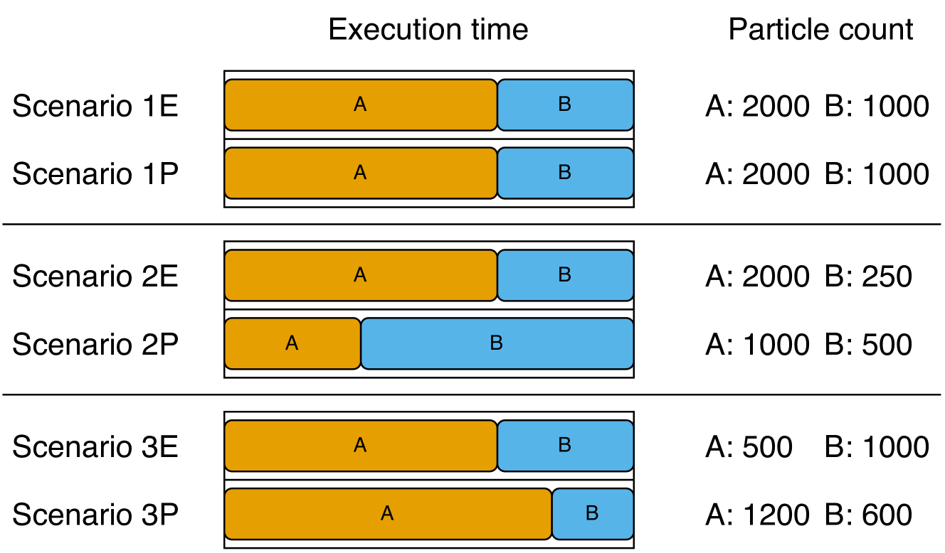Consider Fig. 5, where we present three scenarios to exemplify the differences between execution-time and particle fairness. Assume we have two tasks $\tau_{A}$ and $\tau_{B}$ such that $T_{\tau_{A}}=T_{\tau_{B}}$ and $v_{\tau_{A}}=2\cdot v_{\tau_{B}}$ , running on one core. The tasks are independent and they have the same execution time per particle. We present the outcome of the three scenarios (labeled 1, 2, and 3, respectively) for $\tau_{A}$ and $\tau_{B}$ concerning their relative ratios of execution time and particle count. <details> <summary>x7.png Details</summary>  ### Visual Description ## [Chart Type]: Stacked Bar Chart with Associated Data Table ### Overview The image displays a comparative analysis of six scenarios (1E, 1P, 2E, 2P, 3E, 3P) across two metrics: "Execution time" (represented by stacked horizontal bars) and "Particle count" (listed as numerical values). The chart is organized into three distinct groups separated by horizontal lines. ### Components/Axes * **Primary Headers (Top):** "Execution time" (centered above the bar chart area) and "Particle count" (centered above the numerical data column). * **Row Labels (Left):** Six scenario identifiers: "Scenario 1E", "Scenario 1P", "Scenario 2E", "Scenario 2P", "Scenario 3E", "Scenario 3P". * **Bar Chart Legend (Embedded):** The bars are composed of two colored segments: * **Orange Segment:** Labeled "A" within the bar. * **Blue Segment:** Labeled "B" within the bar. * **Data Column (Right):** For each scenario, lists the particle counts for components A and B in the format "A: [value] B: [value]". ### Detailed Analysis The execution time for each scenario is visualized as a horizontal bar divided into segments A (orange) and B (blue). The total bar length represents the total execution time, and the segment lengths represent the relative time contribution of each component. The numerical particle counts are provided for direct reference. **Group 1 (Top):** * **Scenario 1E:** * Execution Time Bar: Orange segment (A) is longer than the blue segment (B). Approximate visual ratio A:B ~ 2:1. * Particle Count: A: 2000, B: 1000. * **Scenario 1P:** * Execution Time Bar: Identical in appearance to Scenario 1E. Orange segment (A) longer than blue (B). Approximate visual ratio A:B ~ 2:1. * Particle Count: A: 2000, B: 1000. **Group 2 (Middle):** * **Scenario 2E:** * Execution Time Bar: Orange segment (A) is significantly longer than the blue segment (B). Approximate visual ratio A:B ~ 8:1. * Particle Count: A: 2000, B: 250. * **Scenario 2P:** * Execution Time Bar: Blue segment (B) is significantly longer than the orange segment (A). Approximate visual ratio A:B ~ 1:4. * Particle Count: A: 1000, B: 500. **Group 3 (Bottom):** * **Scenario 3E:** * Execution Time Bar: Orange segment (A) is longer than the blue segment (B). Approximate visual ratio A:B ~ 3:2. * Particle Count: A: 500, B: 1000. * **Scenario 3P:** * Execution Time Bar: Orange segment (A) is longer than the blue segment (B). Approximate visual ratio A:B ~ 4:1. * Particle Count: A: 1200, B: 600. ### Key Observations 1. **Identical Pairs:** Scenarios 1E and 1P are visually and numerically identical in both execution time distribution and particle counts. 2. **Inverse Relationship in Group 2:** Scenario 2E shows a very long A segment with high A particles (2000) and low B particles (250). In contrast, Scenario 2P shows a very long B segment with lower A particles (1000) and higher B particles (500) compared to 2E. This suggests a potential performance inversion or different optimization focus. 3. **Particle Count vs. Time Discrepancy:** The relationship between particle count and execution time segment length is not consistent. For example: * In 3E, B has double the particles of A (1000 vs 500) but a shorter execution time segment. * In 3P, A has double the particles of B (1200 vs 600) and a much longer execution time segment. 4. **Grouping:** The scenarios are grouped in pairs (1E/1P, 2E/2P, 3E/3P), suggesting a comparison between two methods or configurations (denoted by 'E' and 'P') for three different base cases. ### Interpretation This chart likely compares the performance (execution time) and resource usage (particle count) of two different algorithms, methods, or system configurations (labeled 'E' and 'P') across three test cases or problem instances (1, 2, 3). * **What the data suggests:** The 'E' and 'P' configurations behave very differently depending on the scenario. In scenario 1, they perform identically. In scenario 2, they show a dramatic trade-off: 'E' spends most time on component A with many A particles, while 'P' spends most time on component B with fewer total particles. In scenario 3, both spend more time on A, but 'P' uses more A particles and achieves a different time distribution. * **How elements relate:** The execution time bar provides a visual, relative measure of where computational effort is spent (A vs. B). The particle count provides an absolute measure of the problem size or data volume for each component. The lack of a direct, consistent correlation between particle count and time segment length implies that the computational cost per particle differs significantly between components A and B, and between the 'E' and 'P' methods. * **Notable anomalies:** The most striking anomaly is the complete reversal of the dominant component (from A in 2E to B in 2P) in the second group. This indicates that the 'P' method might be fundamentally restructured to handle component B differently, or that the problem structure in scenario 2 is uniquely sensitive to the method change. The identical nature of 1E and 1P serves as a control, showing that under some conditions, the methods are equivalent. </details> Figure 5: Illustration of execution time and particle counts for tasks $\tau_{A}$ and $\tau_{B}$ ( $\tau_{A}$ is twice as important as $\tau_{B}$ and both have the same period) for three scenarios when considering execution-time fairness (E) and particle fairness (P). In scenario 1, we find in both cases that, because the tasks have the same execution time per particle, they both end up with the same ratio of execution time and particles. In scenario 2, we assume task $\tau_{B}$ requires four times as much execution time as $\tau_{A}$ per particle. If we use execution-time fairness, the execution time ratio of the tasks remains the same, but $\tau_{B}$ only has time to produce $250$ particles. For particle fairness, the slowdown of $\tau_{B}$ results in both tasks running fewer particles to maintain a fair allocation of particle counts, skewing the execution time in favor of $\tau_{B}$ . In scenario 3, we instead assume $\tau_{A}$ samples from a distribution sent from $\tau_{B}$ , meaning the execution time of $\tau_{A}$ depends on the particle count of $\tau_{B}$ . The exact outcome depends on the ratio of time $\tau_{A}$ spends on sampling. Using execution-time fairness, we find that $\tau_{A}$ only has time to produce $500$ particles. Task $\tau_{B}$ produces the same number of particles as in scenario 1 because it is independent of $\tau_{A}$ . In contrast, when using particle fairness, $\tau_{A}$ produces more particles, and $\tau_{B}$ produces fewer. Which kind of fairness is preferred in a real-time probabilistic inference setting? Although execution-time fairness may seem natural from a real-time perspective, we will see (surprisingly) in the evaluation (Sec. VII-D) that particle fairness works better in practice. Fairness is applicable in scenarios where the output quality is proportional to the time spent producing it. This paper focuses explicitly on SMC inference, where the number of particles controls the quality. However, we foresee no issues extending this to, e.g., MCMC inference algorithms by considering the number of runs instead of the particle count. 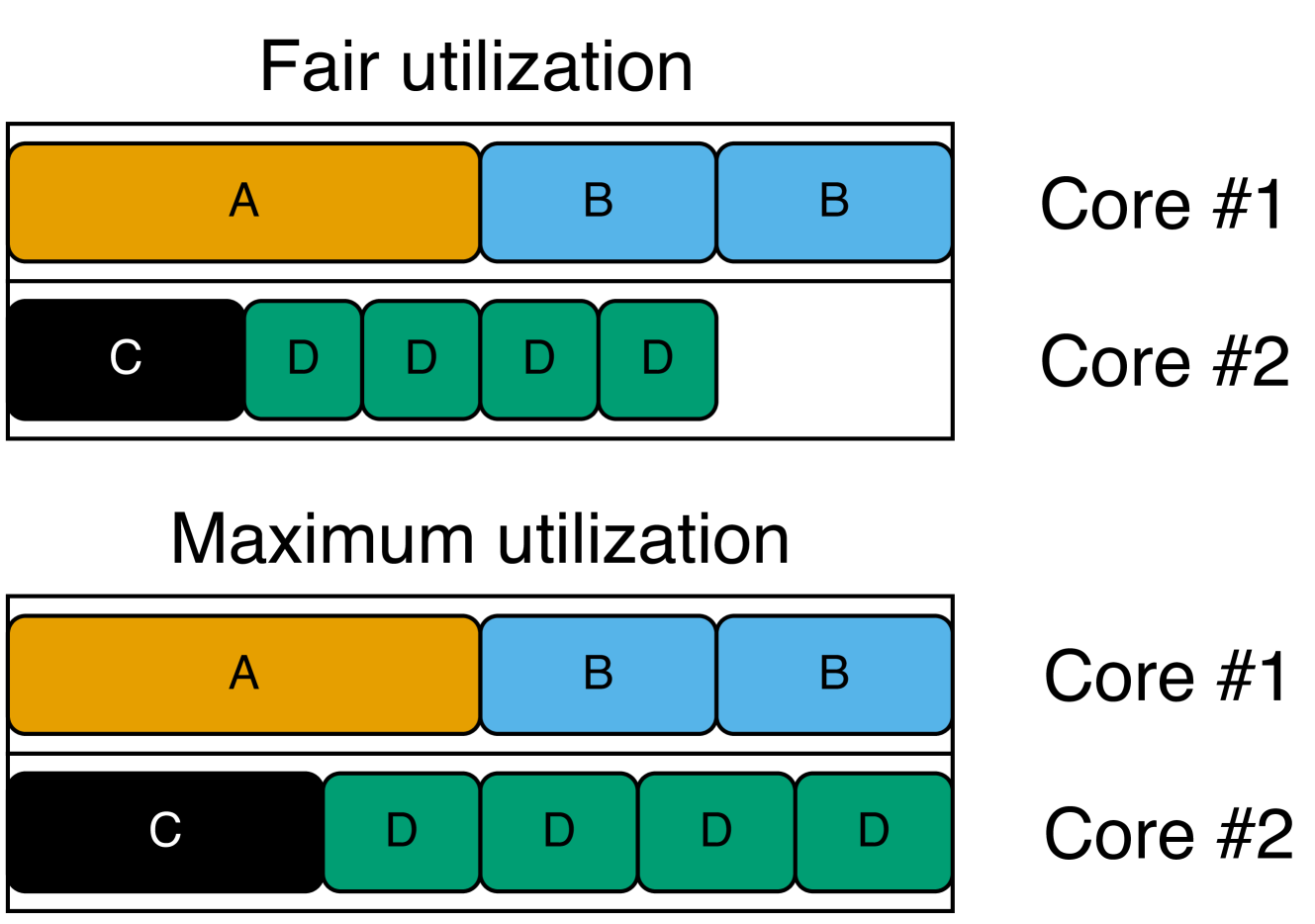### V-B Computation Maximization So far, we only considered the case where tasks run on one core. What if we want to apply fairness to tasks running on multiple cores? We consider two extremes: prioritizing fairness or prioritizing utilization. If we prioritize fairness, we allocate a fixed amount of resources (execution time or particles) to a task instance proportional to its importance value, regardless of which core the task is mapped to. We refer to this as fair utilization. If we prioritize utilization, we maximize the utilization on each core individually, ignoring the importance of tasks running on other cores. We refer to this as maximum utilization. In both cases, the resulting system is schedulable. Assume we allocate the tasks listed on the left-hand side of Fig. 6 on a dual-core system (where $T_{i}$ is the period, $v_{i}$ is the importance, and $c$ is the core of task $\tau_{i}$ ). On the right-hand side, we present the result of applying the two alternatives using execution-time fairness (this also applies to particle fairness). Each box corresponds to a task instance ( $\tau_{D}$ has four times the frequency of $\tau_{A}$ ; hence, it has four boxes), and we consider importance values to apply per task instance. We see that $\tau_{A}$ and $\tau_{B}$ are allocated the same execution time, as $\tau_{A}$ is twice as important as $\tau_{B}$ , but $\tau_{B}$ runs twice as frequently. The main takeaway from Fig. 6 is that, when prioritizing fair utilization, all cores are not always fully utilized. Recall that the tasks of the system may depend on each other. Increasing the execution times of $\tau_{C}$ and $\tau_{D}$ may negatively impact the performance of $\tau_{A}$ and $\tau_{B}$ . This is unfair, considering that $\tau_{A}$ and $\tau_{B}$ have higher importance. On the other hand, if the tasks are independent (which they are in this example), we are wasting computational resources. As an alternative, we also propose the concept of fair utilization maximization, where we start from fair utilization and gradually increase the resources (execution time or particles) allocated to tasks on cores that are not fully utilized as long as the system remains schedulable. If $\tau_{A}$ and $\tau_{B}$ do not depend on $\tau_{C}$ and $\tau_{D}$ , we get the same result as when prioritizing maximum utilization. | $A$ $B$ $C$ | $1\text{\,}\mathrm{s}$ $0.5\text{\,}\mathrm{s}$ $1\text{\,}\mathrm{s}$ | 8 4 4 | 1 1 2 | | --- | --- | --- | --- | | $D$ | $0.25\text{\,}\mathrm{s}$ | 2 | 2 | <details> <summary>x8.png Details</summary>  ### Visual Description ## Diagram: CPU Core Task Allocation Schemes ### Overview The image is a technical diagram illustrating two different task scheduling or resource allocation strategies on a dual-core processor. It visually compares "Fair utilization" and "Maximum utilization" by showing how tasks (labeled A, B, C, D) are distributed across Core #1 and Core #2. The diagram uses colored blocks to represent tasks and their relative execution time or resource consumption. ### Components/Axes The diagram is divided into two primary horizontal sections, each with a title: 1. **Top Section Title:** "Fair utilization" 2. **Bottom Section Title:** "Maximum utilization" Each section contains two horizontal rows representing processor cores: * **Row Label (Right Side):** "Core #1" (top row in each section) * **Row Label (Right Side):** "Core #2" (bottom row in each section) **Task Blocks (Legend by Color and Label):** * **Orange Block:** Labeled "A" * **Light Blue Block:** Labeled "B" * **Black Block:** Labeled "C" * **Green Block:** Labeled "D" ### Detailed Analysis **1. Fair utilization (Top Section):** * **Core #1:** Contains three contiguous blocks. From left to right: one orange "A" block, followed by two light blue "B" blocks. * **Core #2:** Contains five blocks with a visible gap. From left to right: one black "C" block, followed by four green "D" blocks. There is a significant empty white space to the right of the last "D" block, indicating idle time or unused capacity on Core #2. **2. Maximum utilization (Bottom Section):** * **Core #1:** Identical to the "Fair utilization" scheme. Contains one orange "A" block followed by two light blue "B" blocks. * **Core #2:** Contains five contiguous blocks with no gaps. From left to right: one black "C" block, followed by four green "D" blocks. The blocks extend to the far right edge of the row, indicating the core is fully occupied with no idle time. ### Key Observations * **Core #1 Consistency:** The task allocation for Core #1 (A, B, B) is identical in both utilization schemes. * **Core #2 Variance:** The critical difference lies in Core #2. Under "Fair utilization," the four "D" tasks are scheduled with a gap, leaving the core underutilized. Under "Maximum utilization," the same "D" tasks are scheduled back-to-back, filling the core's timeline completely. * **Task Composition:** The workload consists of one "A" task, two "B" tasks, one "C" task, and four "D" tasks, totaling eight discrete task units across two cores. ### Interpretation This diagram demonstrates a fundamental trade-off in system scheduling between fairness and efficiency. * **What it suggests:** The "Fair utilization" model likely represents a scheduling policy that prioritizes equitable access or prevents task starvation, potentially by inserting delays or time-slicing, which results in fragmented execution and idle core time (the gap on Core #2). The "Maximum utilization" model represents a policy focused on throughput and resource efficiency, packing tasks tightly to eliminate idle time, which may come at the cost of fairness or increased latency for some tasks. * **Relationship between elements:** The identical layout of Core #1 implies that the scheduling policy change primarily affects how the "D" tasks (and possibly the "C" task) are handled on Core #2. The "D" tasks appear to be the variable element whose scheduling flexibility allows for the gap in one scheme and the tight packing in the other. * **Notable implication:** The diagram visually argues that the "Maximum utilization" scheme achieves higher overall system throughput (less wasted time) by optimizing the schedule on Core #2, while the "Fair utilization" scheme sacrifices some efficiency, possibly to meet other quality-of-service or fairness guarantees. The choice between them depends on whether the system's goal is to maximize raw performance or ensure balanced resource access. </details> Figure 6: The resulting utilization of the tasks (left) allocated on two cores when prioritizing fairness (top right) or maximizing the utilization (bottom right) in terms of execution time. ## VI Automatic Configuration In this section, we present two approaches to automatic configuration that we apply to a compiled ProbTime system to maximize inference accuracy while preserving schedulability. Automatic configuration is performed before running the system so it does not introduce runtime overheads. ### VI-A Configuration Overview We define two key phases needed to configure a ProbTime system: (i) the collection phase, where we record sensor inputs, and (ii) the configuration phase, where we determine the particle counts of all tasks. During phase (i), we collect input data from the sensors of the actual system, which we replay repeatedly during (ii) in a hardware-in-the-loop simulation. The configuration phase runs on the target system. This paper focuses on the configuration phase (ii). We present two alternative approaches to automatic configuration based on execution-time fairness (Sec. VI-B) and particle fairness (Sec. VI-C). In both cases, we seek a particle count $n_{\tau}$ to use in the inference of each task $\tau$ based on its importance value $v_{\tau}$ , using fair utilization. For simplicity, we assume the user provides a task-to-core mapping $\mathcal{M}$ specifying on which core each task runs (such that $\mathcal{M}_{\tau}\in\mathcal{U}$ ). Also, we assume the existence of a function RunTasks that runs the tasks with pre-recorded sensor data to measure the WCET $W_{\tau}$ of each task $\tau$ . Finally, we use a configurable safety margin factor $\delta$ to protect against outliers in the WCET observations. ### VI-B Execution-Time Fairness We perform two steps to achieve execution-time fairness. First, we compute fair execution time budgets $B_{\tau}$ for each task $\tau$ based on its importance $v_{\tau}$ , such that all tasks remain schedulable. Second, we maximize the particle counts while ensuring the WCET of each task $\tau$ is within its budget. We define the ComputeBudgets function in Algorithm 3 (lines 1 - 6) to compute the execution time budgets of tasks with fair utilization. Our approach assumes partitioned scheduling, which means we can examine tasks assigned to different cores independently. For each core $c_{i}$ , we use the sensitivity analysis in the C-space of Bini et al. [29] to compute a maximum change $\lambda_{i}$ to the execution times of tasks for which they remain schedulable, given a direction vector $\mathbf{d}$ (initially, we assume all execution times are zero). We define $\mathbf{d}$ based on the importance values of the tasks (line 3) and pass it to the SensitivityAnalysis function to compute $\lambda_{i}$ (line 4). Then, we pick the minimum lambda among all cores (line 5) and use this to get fair execution time budgets for all tasks (line 6). Algorithm 3 Function to determine the number of particles to use for execution-time fairness. 1: function ComputeBudgets ( $\mathcal{M},\mathcal{T}$ ) 2: for $c_{i}\in\mathcal{U}$ do 3: $\mathbf{d}\leftarrow\{v_{\tau}\ |\ \tau\in\mathcal{T}\land\mathcal{M}_{\tau}=c _{i}\}$ 4: $\lambda_{i}\leftarrow\textsc{SensitivityAnalysis}(\mathbf{d})$ 5: $\lambda\leftarrow\min_{i}\lambda_{i}$ 6: $\mathbf{return}\ \{(\tau,v_{\tau}\cdot\lambda)\ |\ \tau\in\mathcal{T}\}$ 7: function Configure EF ( $\mathcal{M},\mathcal{T}$ ) 8: $L,U\leftarrow\{(\tau,1)\ |\ \tau\in\mathcal{T}\},\{(\tau,\infty)\ |\ \tau\in \mathcal{T}\}$ 9: $N\leftarrow\{(\tau,1)\ |\ \tau\in\mathcal{T}\}$ 10: $A\leftarrow\{\tau\ |\ \tau\in\mathcal{T}\land P_{\tau}=\emptyset\}$ 11: $B\leftarrow\textsc{ComputeBudgets}(\mathcal{M},\mathcal{T})$ 12: $F\leftarrow\{\tau\ |\ \tau\in\mathcal{T}\land v_{\tau}=0\}$ 13: while $A\neq\emptyset$ do 14: $W\leftarrow\textsc{RunTasks}(\mathcal{M},\mathcal{T})$ 15: for $\tau\in A$ do 16: if $L_{\tau}+1<U_{\tau}$ then 17: $L_{\tau},U_{\tau}\leftarrow\begin{cases}L_{\tau},N_{\tau}&\text{if }\frac{W_{ \tau}}{\delta}>B_{\tau}\\ N_{\tau},U_{\tau}&\text{otherwise}\end{cases}$ 18: $N_{\tau}\leftarrow\begin{cases}2\cdot L_{\tau}&\text{if }U_{\tau}=\infty\\ \lfloor\frac{L_{\tau}+U_{\tau}}{2}\rfloor&\text{otherwise}\end{cases}$ 19: else $N_{\tau},F\leftarrow L_{\tau},F\cup\{\tau\}$ 20: $A\leftarrow\{\tau\ |\ \tau\in\mathcal{T}\land P_{\tau}\subseteq F\}\setminus F$ 21: $\mathbf{return}\ N$ Algorithm 4 Computing the number of particles to use for particle fairness. 1: function Schedulable ( $\mathcal{M},\mathcal{T},k$ ) 2: for $\tau\in\mathcal{T}$ do $n_{\tau}\leftarrow\lfloor k\cdot\overline{v}_{\tau}\rfloor$ 3: $W\leftarrow\textsc{RunTasks}(\mathcal{M},\mathcal{T})$ 4: for $(\tau,W_{\tau})\in W$ do $C_{\tau}\leftarrow\frac{W_{\tau}}{\delta}$ 5: $\textbf{return}\ \textsc{RTA}(\mathcal{M},\mathcal{T})$ 6: function Configure PF ( $\mathcal{M},\mathcal{T}$ ) 7: $L,U\leftarrow 1,\infty$ 8: while $L+1<U$ do 9: $k\leftarrow\begin{cases}2\cdot L&\text{if }U=\infty\\ \lfloor\frac{L+U}{2}\rfloor&\text{otherwise}\end{cases}$ 10: $L,U\leftarrow\begin{cases}k,U&\text{if }\textsc{Schedulable}(\mathcal{M}, \mathcal{T},k)\\ L,k&\text{otherwise}\end{cases}$ 11: $\textbf{return}\ \{(\tau,\lfloor L\cdot\overline{v}_{\tau}\rfloor)\ |\ \tau\in \mathcal{T}\}$ We use the execution time budget $B_{\tau}$ as an upper bound for the WCET of the task $\tau$ while trying to maximize its particle count $n_{\tau}$ . We need to carefully adjust the particle counts of tasks, as they may depend on each other. Assume we have a maximum particle count $n_{\tau}$ for a task $\tau$ . Increasing the particle count of a predecessor task $\tau^{\prime}$ of $\tau$ causes the execution time of $\tau$ to increase. However, if we keep the particle count of all predecessors fixed, the WCET $C_{\tau}$ of a task $\tau$ is proportional to its particle count $n_{\tau}$ . This enables using binary search to find the maximum $n_{\tau}$ . We use these observations in the Configure EF function of Algorithm 3, which returns the particle count $N_{\tau}$ to use for each task $\tau$ . We keep track of a set of active tasks $A$ with no active predecessors (initialized on line 10). We use $P_{\tau}$ to denote the set of predecessors of a task $\tau$ . Note on line 12 that the finished set $F$ is initialized to contain all tasks with importance zero (tasks $\tau$ that perform no inference are assumed to have $v_{\tau}=0$ ). While we have active tasks, we use the RunTasks function to measure the WCETs of all tasks (line 14). We keep track of lower and upper bounds, $L_{\tau}$ and $U_{\tau}$ , of the particle count for each task $\tau$ . For each active task $\tau$ , we compare its measured WCET $W_{\tau}$ to its budget $B_{\tau}$ and update the bounds accordingly (lines 16 - 19). When the binary search concludes, we set the particle count $N_{\tau}$ to the lower bound and add the task $\tau$ to the set of finished tasks $F$ (line 19). At the end of each iteration, we update the set of active tasks (line 20). When the active set $A$ is empty, the resulting particle counts $N$ are returned. Note that the algorithm assumes that the task dependency graph is acyclic. ### VI-C Particle Fairness To achieve particle fairness, we seek a multiple $k$ such that $n_{\tau}=\lfloor k\cdot\overline{v}_{\tau}\rfloor$ for all tasks $\tau$ , where $\overline{v}_{\tau}$ is the normalized importance value . When we increase the value of $k$ , the execution time of all tasks increases, meaning we can binary search to find the maximum $k$ . For a given $k$ , we need to determine whether the tasks are schedulable. We do this in the Schedulable function on lines 1 - 5 of Algorithm 4. We set the number of particles for each task (line 2) and run them (line 3). Then, we set the WCET $C_{\tau}$ of the tasks based on their measured WCETs (line 4) and perform a response time analysis [29] to ensure the tasks are schedulable (line 5). We use the Schedulable function in the particle fairness function Configure PF (lines 6 - 11). We define the lower and upper bounds $L$ and $U$ on line 7, and we binary search in this interval on lines 8 - 10. After the loop, the maximum multiple for which the system is schedulable is stored in $L$ . Based on this, we compute the particle count of each $\tau$ on line 11. ## VII Automotive Case Study To demonstrate the applicability of ProbTime to program time-critical embedded systems, we develop a case study for a localization pipeline in an automotive testbed. This section first introduces the testbed, followed by an evaluation of ProbTime. ### VII-A Automotive Testbed The automotive industry is undergoing a paradigm shift to face the challenges that emerge through the advent of autonomous driving [30]. These challenges require higher computational capacities and larger communication bandwidth than traditional automotive systems. This transition leads to a software-defined vehicle where almost all functions of the car will be enabled by software [31]. To demonstrate the applicability of our proposed methods in this context, we have developed an automotive testbed. #### VII-A 1 Hardware The testbed is designed around a 1:10 scale RC car. The E/E architecture consists of several distributed compute nodes of different characteristics connected via bus- and network-based interconnects (see Fig. 7). 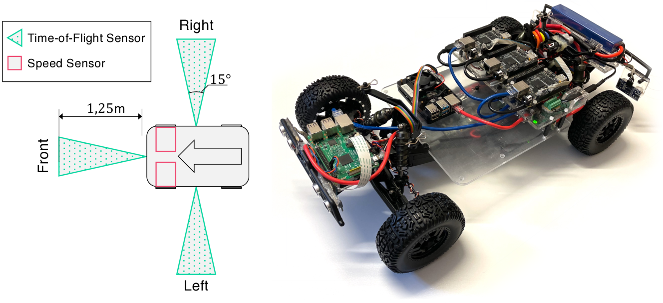<details> <summary>x9.png Details</summary>  ### Visual Description ## Technical Diagram and Photograph: Robotic Vehicle Sensor Configuration ### Overview The image is a composite of two parts: a technical schematic diagram on the left and a photograph of a physical robotic vehicle on the right. The diagram illustrates the placement and field of view of sensors on a vehicle platform, while the photograph shows the actual implementation of a similar robotic car. ### Components/Axes **Left Diagram - Schematic:** * **Legend (Top-Left):** * Cyan triangle symbol: "Time-of-Flight Sensor" * Pink square symbol: "Speed Sensor" * **Vehicle Diagram (Center):** * A top-down view of a rectangular vehicle body with rounded corners. * A large grey arrow inside the vehicle points to the left, indicating the forward direction. * **Front:** A cyan triangle (Time-of-Flight Sensor) is mounted on the front, projecting a dotted cyan cone forward. The cone's range is labeled "1,25m" (1.25 meters). * **Right:** A cyan triangle (Time-of-Flight Sensor) is mounted on the right side, projecting a dotted cyan cone sideways. The cone's angular width is labeled "15°". * **Left:** A cyan triangle (Time-of-Flight Sensor) is mounted on the left side, projecting a dotted cyan cone sideways. No angle is explicitly labeled for this cone, but it is visually symmetric to the right sensor. * **Speed Sensors:** Two pink squares (Speed Sensors) are mounted on the front axle area, one on each side. * **Directional Labels:** "Front", "Right", and "Left" are labeled in black text around the vehicle diagram. **Right Photograph - Physical Robot:** * **Chassis:** A transparent acrylic or polycarbonate base plate. * **Wheels:** Four large, black, knobby rubber tires. * **Electronics:** * A green Raspberry Pi single-board computer is mounted near the front-left wheel. * A larger black circuit board (likely a motor controller or main interface board) is mounted centrally. * A blue lithium polymer (LiPo) battery pack is secured at the rear. * **Wiring:** A complex network of red, black, blue, and multicolored ribbon cables connects the components. * **Sensors:** Several small sensor modules are visible, particularly near the front and sides, consistent with the diagram's layout. Their exact type cannot be confirmed from the photo alone. * **Other Components:** Black suspension components, motor housings, and a front bumper/skid plate. ### Detailed Analysis **Sensor Configuration (from Diagram):** * **Time-of-Flight Sensors (Cyan):** Three sensors are deployed for spatial awareness. 1. **Front Sensor:** Has a specified detection range of 1.25 meters directly ahead. 2. **Side Sensors (Left & Right):** Each has a specified field of view of 15 degrees, oriented perpendicular to the vehicle's body for side obstacle detection. * **Speed Sensors (Pink):** Two sensors are co-located at the front axle, likely for measuring wheel rotation to determine vehicle speed and odometry. **Physical Implementation (from Photograph):** * The robot is a custom-built, four-wheel-drive platform. * The Raspberry Pi suggests it runs a Linux-based operating system for high-level control. * The central board likely handles power distribution and motor control. * The sensor placement on the physical robot appears to align with the schematic, with modules visible at the front and sides. ### Key Observations 1. **Diagram-Photo Correlation:** The schematic provides the design intent (sensor types, placement, and specifications), while the photograph shows the practical, assembled result. The physical robot's sensor locations appear consistent with the diagram. 2. **Sensor Specialization:** The design uses different sensor types for different tasks: Time-of-Flight for distance measurement and obstacle detection, and dedicated speed sensors for motion tracking. 3. **Asymmetry in Labeling:** While the left and right Time-of-Flight sensors are drawn symmetrically, only the right sensor's field of view (15°) is explicitly labeled. It is reasonable to assume the left sensor has an identical specification. 4. **Power System:** The presence of a large LiPo battery indicates the robot is designed for untethered, mobile operation. ### Interpretation This image pair documents the sensor architecture for an autonomous or semi-autonomous ground vehicle. The diagram is a technical specification for sensor integration, defining the robot's perceptual capabilities: * The **front Time-of-Flight sensor** provides long-range forward detection (1.25m), crucial for navigation and collision avoidance. * The **side Time-of-Flight sensors** with their 15-degree fields of view enable the robot to perceive its environment laterally, allowing for tasks like wall-following or navigating through narrow passages. * The **dual front speed sensors** provide redundancy and accuracy for calculating distance traveled (odometry), which is fundamental for localization and motion control. The photograph validates that this design has been physically realized. The use of a Raspberry Pi points to a research or prototyping context, where flexibility and software control are prioritized. The overall system is designed to give the robot a comprehensive, multi-directional understanding of its immediate surroundings, which is the foundational requirement for any autonomous mobile system. The clear documentation (diagram) alongside the implementation (photo) is typical of engineering projects for reproducibility and analysis. </details> Figure 7: Overview of the sensors on the car (left) and a picture of the RC-Car testbed (right). Two microcontroller-based compute nodes act as the interface to most actuators and sensors of the car. High-performance compute nodes provide the required performance to host computation required for Advanced Driving Assistance (ADAS) or Autonomous Driving (AD) workloads. We use a Raspberry Pi 4B (4 Cortex-A72 cores at 1.5GHz). These compute nodes are connected by a local Ethernet network. We use three Time-of-Flight (TOF) sensors installed on the car, as indicated in Fig. 7. These sensors have high accuracy but can only measure distances up to $1.25~{}\text{m}$ . The front wheel sensors report the current speed of the car. 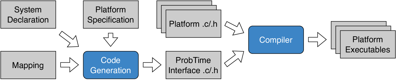#### VII-A 2 Software <details> <summary>x10.png Details</summary>  ### Visual Description ## Diagram: Software Compilation Workflow ### Overview The image is a technical flowchart illustrating a software build or compilation process. It depicts the transformation of high-level system specifications and mappings into platform-specific executable files through a series of defined steps involving code generation and compilation. ### Components/Axes The diagram consists of rectangular boxes representing processes, files, or inputs, connected by directional arrows indicating the flow of data or control. The components are arranged from left to right, generally following the sequence of operations. **Input/Specification Boxes (Gray):** * **System Declaration** (Top-left) * **Mapping** (Bottom-left) * **Platform Specification** (Top-center-left) * **Platform .c/.h** (Top-center, depicted as a stack of three overlapping files) * **ProbTime Interface .c/.h** (Bottom-center) **Process Boxes (Blue):** * **Code Generation** (Center-left) * **Compiler** (Center-right) **Output Box (Gray):** * **Platform Executables** (Far-right, depicted as a stack of three overlapping files) **Flow Arrows:** * Arrows connect the boxes to show the direction of the workflow. ### Detailed Analysis The workflow proceeds as follows: 1. **Inputs to Code Generation:** * The **System Declaration** box has an arrow pointing diagonally down-right to the **Code Generation** box. * The **Mapping** box has an arrow pointing directly right to the **Code Generation** box. * The **Platform Specification** box has an arrow pointing directly down to the **Code Generation** box. * *Interpretation:* The "Code Generation" process consumes three distinct inputs: a system declaration, a mapping definition, and a platform specification. 2. **Code Generation Output:** * The **Code Generation** box has an arrow pointing directly right to the **ProbTime Interface .c/.h** box. * *Interpretation:* The primary output of the code generation step is a set of C source and header files (.c/.h) that form the "ProbTime Interface." 3. **Inputs to Compiler:** * The **Platform .c/.h** file stack has an arrow pointing diagonally down-right to the **Compiler** box. * The **ProbTime Interface .c/.h** box has an arrow pointing diagonally up-right to the **Compiler** box. * *Interpretation:* The compiler takes two sets of source code as input: pre-existing platform-specific files ("Platform .c/.h") and the newly generated interface files ("ProbTime Interface .c/.h"). 4. **Compilation Output:** * The **Compiler** box has an arrow pointing directly right to the **Platform Executables** file stack. * *Interpretation:* The final step of the process is the compilation of all source code into platform-specific executable files. ### Key Observations * **Color Coding:** The two active processing steps ("Code Generation" and "Compiler") are highlighted in blue, distinguishing them from static inputs and outputs (gray). * **File Representation:** Both input source files ("Platform .c/.h") and output executables ("Platform Executables") are shown as stacks of three overlapping rectangles, suggesting multiple files of each type are involved. * **Linear Flow with Parallel Inputs:** The overall flow is linear from left to right, but the "Compiler" stage has two parallel input streams (generated interface code and platform code). ### Interpretation This diagram represents a **model-driven or specification-based software build pipeline**, likely for an embedded or real-time system (suggested by the term "ProbTime"). * **What it demonstrates:** It shows how abstract system definitions ("System Declaration," "Mapping," "Platform Specification") are automatically transformed ("Code Generation") into concrete implementation code ("ProbTime Interface .c/.h"). This generated code is then combined with platform-specific source code ("Platform .c/.h") and compiled into the final runnable binaries ("Platform Executables"). * **Relationships:** The process emphasizes separation of concerns. System logic and mapping are defined separately from the platform specification. The code generation step bridges this gap, creating a platform-agnostic interface. The final compilation step merges this interface with low-level platform code. * **Notable Aspects:** The presence of "ProbTime Interface" suggests the system may be related to probabilistic or real-time computing. The workflow automates a significant portion of the development process, reducing manual coding effort and potential errors by generating interface code from higher-level models. The diagram does not show a feedback loop, indicating this is a one-way, forward engineering process. </details> Figure 8: Code generation and compilation of the platform code, including a ProbTime interface. The operating system on the Raspberry Pi 4B compute node is Linux-based with kernel 5.15.55-rt48-v8+ SMP PREEMPT_RT. The platform software is responsible for reading sensor data and controlling actuators. This is realized by dedicated periodic tasks distributed on different compute nodes. Each task is assigned a static priority and is mapped to a CPU core. Platform software realizes communication between ProbTime tasks by communication buffers located in shared memory. Additionally, sensor data is written to ProbTime communication buffers and from buffers to actuators. We use code generation to produce the files that constitute the interface to a specific ProbTime program (see Fig. 8). Input to the code generation is the system declaration describing the ProbTime program. The remaining platform software is not affected by code generation. The compiler produces an executable for each compute node in the final step. ### VII-B Evaluation Questions To evaluate ProbTime and our automatic configuration, we pose the following evaluation questions: 1. To what extent can ProbTime’s timing and probabilistic constructs be used to implement a realistic application? 1. What is the trade-off between the number of particles, execution time, and inference accuracy? 1. How does execution-time fairness compare to particle fairness concerning allocation of particles and inference time when varying the importance of tasks? 1. To what extent and accuracy can the case study—when executed on the physical car—determine the position and avoid collision? ### VII-C Positioning and Braking in ProbTime (Q1) We implement a positioning and braking system in ProbTime as a case study. The system estimates the position of the RC car while it is moving using sensor inputs. Further, the system reacts by braking to prevent collisions with obstacles. We present an overview of our positioning and braking system in Fig. 9. The figure shows the sensor inputs on the left-hand side. The steering angle is an input signal from the controller, while the other five sensors are directly related to sensors on the car (as shown in Fig. 7). We use the brake actuator (right-hand side) to activate the emergency brakes. 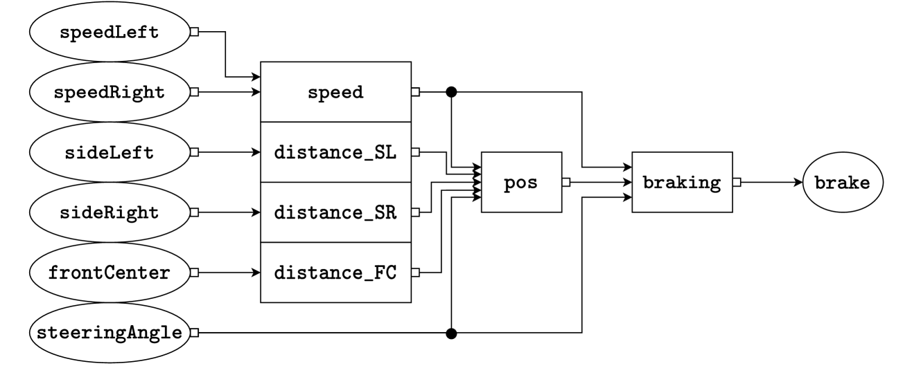<details> <summary>x11.png Details</summary>  ### Visual Description ## Diagram: Vehicle Sensor Fusion and Braking Control System ### Overview The image displays a technical block diagram illustrating a data flow or control system, likely for an autonomous or advanced driver-assistance vehicle. It maps sensor inputs through processing stages to a final braking actuator output. The diagram uses ovals for input/output nodes and rectangles for processing blocks, connected by directional arrows. ### Components/Axes **Input Nodes (Ovals, Left Side):** * `speedLeft` * `speedRight` * `sideLeft` * `sideRight` * `frontCenter` * `steeringAngle` **Processing Blocks (Rectangles, Center):** * `speed` (receives `speedLeft` and `speedRight`) * `distance_SL` (receives `sideLeft`) * `distance_SR` (receives `sideRight`) * `distance_FC` (receives `frontCenter`) * `pos` (receives outputs from `speed`, `distance_SL`, `distance_SR`, `distance_FC`, and `steeringAngle`) * `braking` (receives output from `pos`) **Output Node (Oval, Right Side):** * `brake` ### Detailed Analysis / Content Details **Data Flow and Connections:** 1. **Input Layer:** Six sensor inputs are defined. `speedLeft` and `speedRight` are paired, as are `sideLeft`/`sideRight`. `frontCenter` and `steeringAngle` are singular inputs. 2. **First Processing Stage:** Inputs are routed to dedicated processing blocks: * `speedLeft` & `speedRight` → `speed` block. * `sideLeft` → `distance_SL` block. * `sideRight` → `distance_SR` block. * `frontCenter` → `distance_FC` block. 3. **Sensor Fusion Stage:** The outputs from all four first-stage blocks (`speed`, `distance_SL`, `distance_SR`, `distance_FC`) are fed into the `pos` block. The `steeringAngle` input also connects directly to the `pos` block, bypassing the first stage. 4. **Decision & Actuation Stage:** The `pos` block outputs to the `braking` block. The `braking` block's output connects to the final `brake` actuator node. **Spatial Grounding:** * Inputs are vertically stacked on the far left. * The first-stage processing blocks are vertically stacked in the center-left. * The `pos` block is centrally located. * The `braking` block is to the right of `pos`. * The final `brake` output is on the far right. * All connections are indicated by solid black lines with arrowheads showing flow direction from left to right. ### Key Observations * **Hierarchical Processing:** The system has a clear two-stage processing architecture before the final braking decision. * **Direct Steering Input:** The `steeringAngle` has a unique, direct connection to the `pos` block, suggesting it is a critical parameter for position/state calculation, not just a distance or speed metric. * **Symmetry:** Inputs for left/right sides (`speedLeft/Right`, `sideLeft/Right`) are processed symmetrically before fusion. * **Single Output:** The entire complex sensor array and processing chain culminates in a single actuator command: `brake`. ### Interpretation This diagram represents a **sensor fusion and control logic pipeline** for a vehicle's automated braking system. The underlying principle is that safe braking decisions (`brake`) depend on a synthesized understanding of the vehicle's state and environment (`pos`). * **What it demonstrates:** The system fuses dynamic data (wheel speeds), spatial awareness data (side and front distances), and driver intent/vehicle dynamics data (steering angle) to compute a position or state estimate (`pos`). This estimate is then used by a dedicated `braking` controller to determine the appropriate braking action. * **Relationships:** The flow shows a transformation from raw sensor data → processed metrics (speed, distances) → fused situational awareness (`pos`) → control decision (`braking`) → physical actuation (`brake`). The `pos` block is the critical nexus where all information converges. * **Notable Implications:** The architecture implies that braking is not triggered by a single sensor (e.g., front distance alone) but by a holistic assessment. The direct link from `steeringAngle` to `pos` is particularly important, as it indicates the system accounts for the vehicle's trajectory and intended path when calculating its state, which is essential for functions like stability control or predictive emergency braking in curves. The absence of numerical values indicates this is a conceptual or architectural diagram, not a performance chart. </details> Figure 9: A graphical representation of the positioning and braking system. The squares of Fig. 9 represent the tasks. We instantiate all distance estimation tasks (distance_SL, distance_SR, and distance_FC) from the same template. All tasks have a period of $500\text{\,}\mathrm{ms}$ except pos, which has a period of $1\text{\,}\mathrm{s}$ . We use the speed task to estimate the car’s average speed since the last estimation based on speed observations from the wheels. Preliminary experiments show that the speed sensors are inaccurate at low speeds and that the top speed is reached almost instantaneously when accelerating. Due to the predictable behavior of the speed, we model it as being in one of three states: stationary, max speed, or transitioning (either accelerating or decelerating). This is simpler than using Bayesian linear regression (as we did in the speed model in Listing 2) and computationally cheaper. Our positioning task estimates the x- and y-coordinates of the car’s center. It also estimates the direction the car faces relative to an encoded map of the environment (provided by the user). The model starts from a prior belief of the position (initially, a known starting position) and estimates a trajectory along which the car moved until the current logical time of the task based on steering angle observations and speed estimations. We update our belief by comparing each input distance estimation with what the sensor would have observed at that timestamp, given that the car followed the estimated trajectory. We implement this using Bayesian linear regression. The braking task uses a probabilistic model to estimate the distance until a collision occurs, given steering angle observations, an encoded map, and the speed and position estimations. We activate the emergency brakes if the median distance is estimated to be below a fixed threshold. In response to Q1, the current case study demonstrates that a non-trivial application can be efficiently implemented in ProbTime (using 600 lines of code). ### VII-D Experiments and Results To answer evaluation questions Q2, Q3, and Q4, we perform three experiments on the positioning system of Fig. 9. We want to run as many particles per iteration as possible for the first experiment. Therefore, we run this on an Intel(R) Xeon(R) Gold 6148 CPU with 64 GB RAM using Ubuntu 22.04. We use the Raspberry Pi on the car for the second and third experiments. The first two experiments use pre-recorded data in a simulation, while the third uses live data. When discussing results or settings, we only consider the pos and braking tasks, as the other tasks perform no inference. The pos and braking tasks run on separate cores. #### VII-D 1 Positioning Inference Accuracy (Q2) We investigate how the number of particles impacts the inference accuracy and execution times. To be able to run more particles per inference, we perform a slow mode simulation where the replaying of observation data and the ProbTime tasks consider time to pass slower relative to the wall time. We use position estimates as a measure of inference accuracy because they are easily compared to a known final position from pre-recorded data. In this experiment, we vary the particle count of the pos task while fixing the particle count of braking. In Fig. 10, we present the average position error along the x- and y-axis (left) and the WCETs (right) for the two tasks over $100$ runs with varying particle counts in the positioning task. Note that the positioning model often fails to track the car when using $10^{2}$ particles. The estimation error along both axes decreases drastically as we increase the number of particles, mainly when increasing from $10^{2}$ to $10^{3}$ particles. The increased variance going from $10^{4}$ to $10^{5}$ particles is likely due to inaccuracies in our model. The WCET of the pos task scales linearly with the number of particles (note the logarithmic axes), while the braking task becomes noticeably slower when we increase the number of particles to $10^{5}$ . This is because it processes a position distribution sent from the pos task (i.e., braking depends on pos). In connection to Q2, we have seen the impact of particle count on the inference accuracy. Few particles lead to a big uncertainty, and the benefit of increasing the particle count is negligible past a certain point. We also see that the number of particles is linearly connected to the WCET and that the particle count of a task may impact the WCET of other tasks. 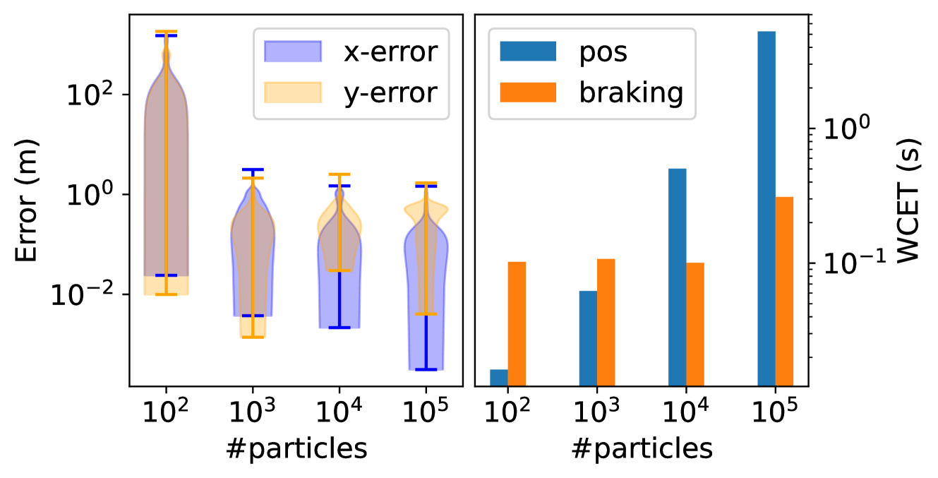<details> <summary>x12.png Details</summary>  ### Visual Description ## [Chart Type]: Dual-Panel Performance Analysis (Violin Plot and Bar Chart) ### Overview The image displays a two-panel figure analyzing the performance of a particle-based system (likely a filter or simulation) as a function of the number of particles. The left panel shows error distributions, and the right panel shows Worst-Case Execution Time (WCET). Both panels share a common x-axis representing the number of particles on a logarithmic scale. ### Components/Axes **Common X-Axis (Both Panels):** * **Label:** `#particles` * **Scale:** Logarithmic * **Markers/Ticks:** `10²`, `10³`, `10⁴`, `10⁵` **Left Panel (Violin Plot):** * **Title/Type:** Violin Plot of Error Distributions * **Y-Axis Label:** `Error (m)` * **Y-Axis Scale:** Logarithmic, ranging from approximately `10⁻²` to `10²` meters. * **Legend:** Located at the top-center of the panel. * `x-error`: Represented by blue-filled violin shapes and blue error bars. * `y-error`: Represented by orange-filled violin shapes and orange error bars. * **Data Representation:** For each particle count (`10²`, `10³`, `10⁴`, `10⁵`), there are two overlapping violin plots showing the probability density of the error data. Vertical lines with horizontal caps (error bars) indicate the range or confidence intervals. **Right Panel (Bar Chart):** * **Title/Type:** Bar Chart of Worst-Case Execution Time (WCET) * **Y-Axis Label:** `WCET (s)` * **Y-Axis Scale:** Logarithmic, ranging from approximately `10⁻¹` to `10⁰` seconds. * **Legend:** Located at the top-left of the panel. * `pos`: Represented by blue bars. * `braking`: Represented by orange bars. * **Data Representation:** For each particle count, two bars are grouped together, showing the WCET for "pos" (likely position computation) and "braking" tasks. ### Detailed Analysis **Left Panel - Error Distributions:** * **Trend Verification:** Both `x-error` (blue) and `y-error` (orange) distributions show a clear trend: as the number of particles increases from `10²` to `10⁵`, the distributions become narrower and shift downward on the logarithmic scale. This indicates a reduction in both the magnitude and variance of the error. * **Data Points & Observations:** * **At 10² particles:** The distributions are very wide, spanning nearly the entire y-axis range. The `y-error` (orange) distribution appears slightly wider and extends to higher error values than the `x-error` (blue). The central tendency (median/mean) for both is around `10⁰` to `10¹` meters. * **At 10³ particles:** A significant reduction in error is visible. The distributions are centered closer to `10⁻¹` meters. The `y-error` distribution still appears slightly broader than the `x-error`. * **At 10⁴ particles:** Error continues to decrease. The distributions are now centered below `10⁻¹` meters. The shapes are more compact. * **At 10⁵ particles:** The error is lowest. The distributions are tightly clustered around `10⁻²` meters. The `x-error` (blue) distribution appears to have a slightly lower median than the `y-error` (orange) at this point. **Right Panel - WCET:** * **Trend Verification:** Both `pos` (blue) and `braking` (orange) WCET show an increasing trend with the number of particles. The increase for `pos` is dramatically steeper than for `braking`. * **Data Points & Approximate Values:** * **At 10² particles:** * `pos` (blue): WCET is very low, approximately `2 x 10⁻²` seconds (0.02 s). * `braking` (orange): WCET is approximately `1.5 x 10⁻¹` seconds (0.15 s). * **At 10³ particles:** * `pos` (blue): Increases to approximately `10⁻¹` seconds (0.1 s). * `braking` (orange): Increases slightly to approximately `2 x 10⁻¹` seconds (0.2 s). * **At 10⁴ particles:** * `pos` (blue): Increases significantly to approximately `2 x 10⁰` seconds (2 s). * `braking` (orange): Remains relatively stable, around `1.5 x 10⁻¹` seconds (0.15 s). * **At 10⁵ particles:** * `pos` (blue): Shows a massive increase, reaching approximately `4 x 10⁰` seconds (4 s). This is the tallest bar in the chart. * `braking` (orange): Increases to approximately `9 x 10⁻¹` seconds (0.9 s). ### Key Observations 1. **Accuracy-Computation Trade-off:** There is a clear inverse relationship between accuracy (error) and computational cost (WCET). Increasing particles from `10²` to `10⁵` reduces error by roughly two orders of magnitude but increases the WCET for the `pos` task by over two orders of magnitude. 2. **Differential Cost Growth:** The computational cost (`WCET`) of the `pos` task scales much more poorly with particle count than the `braking` task. At `10⁵` particles, `pos` WCET is over 4 times greater than `braking` WCET. 3. **Error Convergence:** The error distributions for both x and y dimensions converge to similar, low values at high particle counts (`10⁵`), suggesting the system's accuracy becomes isotropic with sufficient particles. 4. **Initial Instability:** At the lowest particle count (`10²`), the error distributions are extremely wide, indicating highly unreliable and variable performance. ### Interpretation This figure illustrates a classic engineering trade-off in particle-based estimation or simulation systems (e.g., Particle Filters). The data demonstrates that **increasing the number of particles directly improves estimation accuracy (reduces error) but at a significant and non-linear computational cost.** * **What the data suggests:** The system's precision is highly dependent on particle count. The dramatic narrowing of the violin plots shows that more particles lead to more consistent and accurate estimates. However, the bar chart reveals that this accuracy comes at a price, particularly for the `pos` (position) computation, which appears to have a computational complexity that grows super-linearly with the number of particles. * **How elements relate:** The two panels are two sides of the same coin. The left panel shows the *benefit* (lower error), and the right panel shows the *cost* (higher WCET) of scaling up the system. An engineer would use this data to find an optimal operating point—perhaps at `10⁴` particles, where error is already quite low (`~0.1 m`) and the `pos` WCET (`~2 s`) might still be acceptable for a real-time system, whereas at `10⁵` particles, the WCET (`~4 s`) may be prohibitive despite marginally better accuracy. * **Notable Anomalies/Insights:** The most striking insight is the disproportionate growth of the `pos` WCET. This suggests that the algorithm for position computation does not scale efficiently with particle count and could be a bottleneck. Optimizing this specific component would yield the greatest performance gains. The relatively flat WCET for `braking` suggests it is a less complex or fixed-cost operation. The investigation should focus on why `pos` computation is so expensive and whether approximations or algorithmic changes can mitigate this. </details> Figure 10: Results showing the estimation error along the x- and y-axis of the car (left) and the WCETs (right) over ten runs, varying the number of particles in the positioning model. Both figures have a logarithmic x- and y-axis. #### VII-D 2 Automatic Configuration (Q3) To compare the automatic configuration using execution-time and particle fairness, we vary the ratio of importance between the pos and braking tasks. For each ratio, we measure the particle count and WCET of the configured tasks and the number of iterations needed to configure the system. The resulting ratio of particle count and execution time is presented in Fig. 11. In our experiment, we vary the importance ratio between tasks by powers of two until the starting state cannot be scheduled. As expected, both approaches to fairness have one property scaling at the same rate as the importance ratio (WCET ratio for execution-time fairness and particle count ratio for particle fairness). The WCET ratio for particle fairness peaks when the ratio imbalance is too large (e.g., when the ratio is $2^{8}$ ) as the more important task fully utilizes its core. Increasing the ratio imbalance past this point only causes the less important task to run fewer particles. For execution-time fairness, this imbalance results in the less important task being allocated an insufficient budget due to fair utilization. Execution-time fairness needs $48.8\pm 11.8$ iterations (mean and standard deviation) to configure all tasks compared to $16.5\pm 2.8$ for particle fairness. Recall from Sec. VI that execution-time fairness considers task dependencies while particle fairness runs independently of them. For our model, the problem of task dependencies is hardly noticeable. However, what if the speed task also performed inference? To investigate this, we configure a variant of the positioning and braking model where speed performs inference, with it running on a separate core from pos and braking, and all three tasks have the same importance. We find that the tasks all get $385$ particles using particle fairness, whereas using execution-time fairness, pos gets $21$ particles, braking gets $95$ particles, and speed gets $24199$ particles. For execution-time fairness, the speed task has time to run many particles, which slows down the other tasks that depend on its output. This issue could be mitigated by setting an upper bound on the particle count (machine-specific) or by giving pos and braking higher importance. 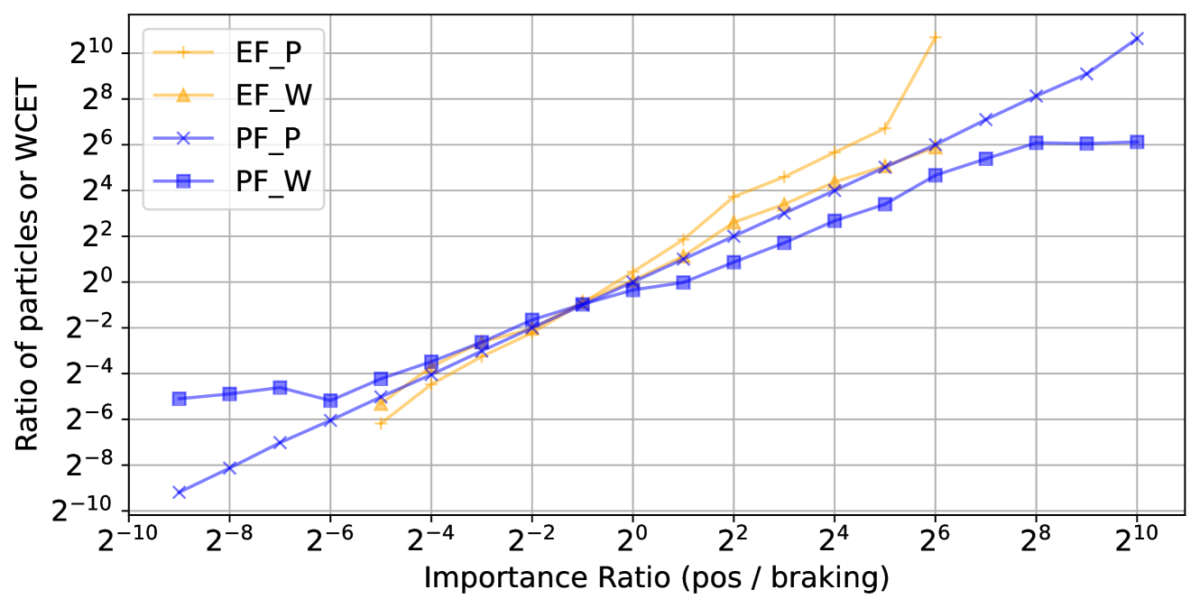<details> <summary>x13.png Details</summary>  ### Visual Description ## Line Chart: Importance Ratio vs. Ratio of Particles or WCET ### Overview This is a line chart plotted on a log-log scale (base 2). It displays the relationship between an "Importance Ratio (pos / braking)" on the x-axis and a "Ratio of particles or WCET" on the y-axis. Four distinct data series are plotted, each representing a different method or condition (EF_P, EF_W, PF_P, PF_W). The chart demonstrates how the output ratio (y-axis) changes as the input importance ratio (x-axis) varies over a wide range. ### Components/Axes * **X-Axis:** * **Label:** `Importance Ratio (pos / braking)` * **Scale:** Logarithmic (base 2). * **Range & Ticks:** From `2^-10` to `2^10`. Major ticks are labeled at every power of 2: `2^-10`, `2^-8`, `2^-6`, `2^-4`, `2^-2`, `2^0`, `2^2`, `2^4`, `2^6`, `2^8`, `2^10`. * **Y-Axis:** * **Label:** `Ratio of particles or WCET` * **Scale:** Logarithmic (base 2). * **Range & Ticks:** From `2^-10` to `2^10`. Major ticks are labeled at every power of 2: `2^-10`, `2^-8`, `2^-6`, `2^-4`, `2^-2`, `2^0`, `2^2`, `2^4`, `2^6`, `2^8`, `2^10`. * **Legend:** * **Position:** Top-left corner of the chart area. * **Entries:** 1. `EF_P`: Yellow line with plus (`+`) markers. 2. `EF_W`: Yellow line with upward-pointing triangle (`▲`) markers. 3. `PF_P`: Blue line with cross (`x`) markers. 4. `PF_W`: Blue line with square (`■`) markers. ### Detailed Analysis **Trend Verification & Data Point Extraction (Approximate Values):** 1. **EF_P (Yellow, `+` markers):** * **Trend:** Shows the steepest upward slope. It starts low, crosses the other lines near the center, and continues to rise sharply, exceeding the chart's upper bound at the highest x-values. * **Key Points (x, y):** (~`2^-5`, ~`2^-6`), (~`2^0`, ~`2^0`), (~`2^2`, ~`2^4`), (~`2^4`, ~`2^6`), (~`2^6`, >`2^10`). 2. **EF_W (Yellow, `▲` markers):** * **Trend:** Follows a similar upward trajectory to EF_P but diverges after `x=2^0`, growing at a slightly slower rate. * **Key Points (x, y):** (~`2^-5`, ~`2^-6`), (~`2^0`, ~`2^0`), (~`2^2`, ~`2^3`), (~`2^4`, ~`2^4`), (~`2^6`, ~`2^6`). 3. **PF_P (Blue, `x` markers):** * **Trend:** Exhibits a consistent, nearly linear upward slope on this log-log plot across the entire range. It starts as the lowest series and ends as one of the highest. * **Key Points (x, y):** (~`2^-9`, ~`2^-10`), (~`2^-6`, ~`2^-6`), (~`2^0`, ~`2^0`), (~`2^4`, ~`2^4`), (~`2^8`, ~`2^8`), (~`2^10`, ~`2^10`). 4. **PF_W (Blue, `■` markers):** * **Trend:** Increases initially but then plateaus. It shows the most significant saturation effect at higher x-values. * **Key Points (x, y):** (~`2^-9`, ~`2^-5`), (~`2^-6`, ~`2^-5`), (~`2^0`, ~`2^0`), (~`2^4`, ~`2^3`), (~`2^6`, ~`2^6`), (~`2^8`, ~`2^6`), (~`2^10`, ~`2^6`). **Component Isolation & Spatial Grounding:** * **Intersection Point:** All four lines converge and intersect in a tight cluster near the chart's center, at approximately `(x=2^0, y=2^0)`. * **Low X-Region (Left, x < 2^0):** The series are ordered from highest to lowest y-value as: PF_W > EF_W ≈ EF_P > PF_P. * **High X-Region (Right, x > 2^4):** The series order changes significantly. EF_P becomes the highest, followed by PF_P, then EF_W, with PF_W being the lowest and flat. ### Key Observations 1. **Divergence After Intersection:** The most notable pattern is the dramatic divergence of the four series after they intersect near `(2^0, 2^0)`. This indicates that the system's behavior is highly sensitive to the "Importance Ratio" around a value of 1. 2. **Saturation of PF_W:** The `PF_W` series clearly saturates, reaching a maximum y-value of approximately `2^6` and not increasing further even as the importance ratio increases by several orders of magnitude. 3. **Super-Linear Growth of EF_P:** The `EF_P` series grows faster than linearly (on the log-log scale) for `x > 2^2`, suggesting a potentially exponential or high-polynomial relationship in that regime. 4. **Consistent Scaling of PF_P:** The `PF_P` series maintains a near-constant power-law relationship (linear on log-log) across the entire 20-order-of-magnitude range of the x-axis. ### Interpretation This chart likely compares the performance or resource usage (measured by "Ratio of particles or WCET") of four different algorithms or system configurations (EF_P, EF_W, PF_P, PF_W) as a key parameter, the "Importance Ratio (pos / braking)," is varied. * **What the data suggests:** The "EF" methods (yellow) appear more sensitive to changes in the importance ratio, especially at higher values, with EF_P showing extreme scaling. The "PF" methods (blue) are more stable, with PF_W being particularly robust (or limited) as it hits a performance ceiling. The intersection at `(1,1)` is a critical operating point where all methods yield the same output ratio. * **How elements relate:** The x-axis parameter acts as a control knob. Moving from left to right (increasing pos/braking importance) generally increases the output ratio for all methods, but the *rate* of increase is the key differentiator. The choice of method (EF vs. PF) and condition (P vs. W) dictates the system's scalability and upper limits. * **Notable Anomalies:** The plateau of `PF_W` is a significant anomaly, indicating a fundamental constraint or optimal operating point for that configuration. The super-linear growth of `EF_P` could be a warning sign of poor scalability or a desired feature for extreme prioritization, depending on the context. The chart effectively visualizes a trade-off: methods that scale aggressively (EF_P) may lack stability, while stable methods (PF_W) may have limited peak performance. </details> Figure 11: The ratio of particles (using suffix P) and worst-case execution time (suffix W) when varying the importance ratio. We use prefix EF for execution-time fairness results and PF for particle fairness. Note the logarithmic x- and y-axes. <details> <summary>extracted/5716520/figures/corridor.png Details</summary>  ### Visual Description ## Diagram: Abstract Geometric Layout ### Overview The image displays a simple, abstract diagram composed of geometric shapes on a solid background. It appears to be a schematic or layout plan, possibly representing a floor plan, a circuit board, or a conceptual block diagram. There is no visible text, numerical data, or chart elements. The composition is minimalist, using two primary colors. ### Components/Axes * **Background:** A solid, light purple (lavender) field. * **Primary Shapes:** Dark purple (near-black) geometric forms. * A large, central horizontal rectangle. * A vertical rectangle on the far left edge. * A smaller vertical rectangle on the far right edge. * A small square in the bottom-left corner. * A small square in the bottom-right area. * A small horizontal rectangle below the central rectangle, slightly left of center. * A small vertical rectangle to the left of the central rectangle, near the top. * A small square above the central rectangle, near the right edge. * **Anomalous Element:** A small, blurry, multicolored (green, blue, yellow) spot is located in the upper-right quadrant, above the central rectangle. Its purpose is unclear; it may be a highlight, an artifact, or a poorly rendered icon. ### Detailed Analysis * **Spatial Arrangement:** The shapes are arranged with a sense of balance but not perfect symmetry. The large central rectangle is the dominant element. The smaller shapes are placed around it, creating a framed or compartmentalized effect. * **Color & Form:** The diagram uses a strict two-color scheme (light purple background, dark purple shapes) except for the anomalous multicolored spot. All shapes have sharp, right-angled corners. * **Scale & Proportion:** The central rectangle occupies approximately 60% of the image's width and 40% of its height. The other shapes are significantly smaller, suggesting they may represent secondary components, connectors, or markers. ### Key Observations 1. **Absence of Text:** The diagram contains zero textual labels, titles, axis markers, or legends. All information is conveyed through shape, color, and spatial relationship. 2. **Abstract Nature:** Without context, the diagram is purely abstract. It does not contain recognizable symbols, flow arrows, or standard schematic icons that would indicate a specific domain (e.g., electrical engineering, architecture). 3. **The Multicolored Spot:** This element is the only one that breaks the strict two-color palette. Its blurry, glowing appearance contrasts with the flat, solid colors of the other shapes, making it a focal point of uncertainty. ### Interpretation * **What the Data Suggests:** As there is no explicit data, the image suggests a **structural or spatial relationship** between components. The layout implies a system where a main module (central rectangle) is surrounded by peripheral elements (smaller shapes), which could represent inputs, outputs, supports, or interfaces. * **How Elements Relate:** The positioning creates a visual hierarchy. The central block is primary. The flanking vertical rectangles on the left and right edges could denote boundaries or major connection points. The smaller squares and rectangles may be subordinate nodes or features. * **Notable Anomalies:** The multicolored spot is the primary anomaly. It could be: * A **highlight** indicating an active area, a point of interest, or a status indicator (e.g., "power on"). * A **rendering error** or artifact from the image creation process. * A **poorly downscaled icon** that lost its detail. Its ambiguity is the most significant feature for interpretation, as it is the only element that breaks the diagram's visual consistency and may hold a key to its meaning if it were legible. **Conclusion:** This image is a low-detail, abstract schematic. Its informational content is limited to the spatial arrangement of simple geometric forms. To extract meaningful technical data, additional context, labels, or a higher-resolution version showing the detail of the multicolored spot would be required. </details> Figure 12: The encoded map ( $18.6\text{\,}\mathrm{m}$ x $9.5\text{\,}\mathrm{m}$ ) of the corridor in which we drive the car. The overlay shows particles spreading when less information is available (top-right) and gathering when close to distinguishable obstacles (bottom-left). In connection to Q3, we argue that particle fairness is preferable. First, the problems above only apply to execution-time fairness. Second, there is a direct connection between particle count and inference accuracy. Therefore, we argue that reasoning about the allocation of particles directly seems more natural than doing it in terms of execution time. #### VII-D 3 Positioning and Braking (Q4) For this experiment, we run the tasks on the physical car. To evaluate the positioning model, we drive the car around in a corridor (Fig. 12). As we measure the car’s position by hand, we can only make measurements when the car is stationary. Therefore, we drive it from a known starting position and compare the actual final position to the last position estimated by the model. We drive the car in a clockwise direction for a full lap ten times using two distinct scenarios to illustrate how environmental details impact the accuracy of the position estimates. In scenario 1, we start at the bottom-left corner and drive past the starting point. In scenario 2, we begin in the top-right corner and stop along the long corridor at the top. During preliminary evaluations, we found that using importance $4$ for pos and $1$ for braking yields good results. The configured system runs inference using $1312$ particles in pos and $328$ in braking. We evaluate the automated braking by driving the car around in the corridor. We find that the emergency brakes are conservative—while they prevent collisions, they often activate in situations where it is unnecessary. This is due to uncertainty in the position estimations. Due to the conservative nature of the braking task, we turn off the brake actuator when evaluating the positioning model. We present the positioning results in Table I. The error along the y-axis is small in scenario 2 because both side sensors are in range in the narrow corridor where the car stops, while the x-axis error is large because the front distance sensor is outside of its range in the corridor. Despite the short range of our sensors, the lack of distinguishing details in the environment, and the limited computational power of the car testbed, our model successfully tracks the car for a full lap in the corridor. Tracking the car in itself is not a novelty, but it shows that the methodology works in practice for a non-trivial application. TABLE I: Results showing the average error in the x- and y-direction (in meters) and the Euclidean distance for our two scenarios, with standard deviations. | 1 2 | $0.50\pm 0.58$ $1.19\pm 0.79$ | $0.28\pm 0.23$ $0.24\pm 0.14$ | $0.63\pm 0.56$ $1.21\pm 0.80$ | | --- | --- | --- | --- | ## VIII Related Work Although surprisingly little has been done in the intersection of probabilistic programming and languages for real-time systems, there is a large body of work in each category. This section gives a summary of the closest related work. Probabilistic programming languages. Languages for performing Bayesian inference date back to the early 1990s, where BUGS [32] is one of the earliest languages for Bayesian networks. The term probabilistic programming was coined much later but is now generally used for all languages performing Bayesian inference. Starting with the Church language [33], a new, more general form of probabilistic programming languages emerged, called universal PPLs. In such languages, the probabilistic model is encoded in a Turing complete language, which enables stochastic branching and possibly an infinite number of random variables. There exist many experimental PPLs in this category, e.g., Gen [11], Anglican [9], Turing [10], WebPPL [7], Pyro [6], and CorePPL [12]. Other state-of-the-art PPL environments are, e.g., Stan [8] and Infer.NET. Similar to many of these environments, ProbTime also makes use of the standard core constructs (sample, observe, and infer), where the key difference is that time and timeliness are also taken into consideration in ProbTime. Real-time programming languages. There exists a quite large body of literature on programming languages that incorporate time and timing as part of the language semantics. Ada [19] has explicit support for timed language constructs, and the real-time extension to Java [34] supports time and event handling. Recently, Timed C was proposed in the research literature to incorporate timing constructs directly in the language. The Timed C work was later extended to support sensitivity analysis [35]. Our work has been inspired by Timed C; the semantics for periodic is loosely based on sdelay in Timed C, although the implementation is different. As in Timed C, ProbTime introduces tagging with timestamps. There are several other languages and environments that have timestamped and tagged values as central semantic concepts. For instance, PTIDES [36] extends the discrete-event (DE) model. Lingua Franca [18] is another recent effort that introduces deterministic actors called reactors, whose only means of communication is through an ordered set of reactions. Synchronous programming. There are also other approaches to programming real-time systems where time is abstracted as ticks. Specifically, the synchronous programming paradigm [37] implements such an approach, where ProbZelus [20] is a recent programming language extending synchronous reactive programming with probabilistic constructs. The ProbZelus work is based on the delayed sampling concept [38] to automatically make inference efficient when conjugate priors can be exposed in the model. A key difference between ProbZelus and ProbTime is our concept of fairness, where the number of particles used in inference is automatically adjusted based on user-provided importance values. Reward-based scheduling. Our automatic configuration is related to reward-based scheduling [39], where tasks consist of a mandatory and an optional part. A non-decreasing reward function maps the time spent running the optional part to a real value. This approach aims to find a schedule for maximizing the reward while all tasks remain schedulable. In ProbTime, inference is the optional part of tasks as we can vary how many particles we use. The importance values assigned to tasks implicitly encode a reward function. ## IX Conclusion In this paper, we introduce a new kind of language called real-time probabilistic programming language (RTPPL). To demonstrate this new kind of language, we develop and analyze a domain-specific RTPPL called ProbTime. We also introduce the concepts of fairness in RTPPLs and illustrate the strength of particle fairness. ## Acknowledgment We would like to thank John Wikman, Linnea Stjerna, Gizem Çaylak, Viktor Palmkvist, Anders Ågren Thuné, Thilanka Thilakasiri, and Rodolfo Jordão for their valuable feedback. This project is financially supported by the Swedish Foundation for Strategic Research (FFL15-0032 and RIT15-0012). The research has also been carried out as part of the Vinnova Competence Center for Trustworthy Edge Computing Systems and Applications (TECoSA) at the KTH Royal Institute of Technology. ## References - [1] A. D. Gordon, T. A. Henzinger, A. V. Nori, and S. K. Rajamani, “Probabilistic programming,” in Proceedings of the on Future of Software Engineering. ACM, 2014, pp. 167–181. - [2] J.-W. van de Meent, B. Paige, H. Yang, and F. Wood, “An introduction to probabilistic programming,” arXiv preprint arXiv:1809.10756, 2018. - [3] A. Doucet, N. De Freitas, and N. Gordon, “An introductiona to sequential Monte Carlo methods,” Sequential Monte Carlo methods in practice, pp. 3–14, 2001. - [4] Lundén, Daniel and Borgström, Johannes and Broman, David, “Correctness of Sequential Monte Carlo Inference for Probabilistic Programming Languages,” in Proceedings of 30th European Symposium on Programming (ESOP), ser. LNCS, vol. 12648. Springer, 2021, pp. 404–431. - [5] S. Brooks, “Markov chain Monte Carlo method and its application,” Journal of the royal statistical society: series D (the Statistician), vol. 47, no. 1, pp. 69–100, 1998. - [6] E. Bingham, J. P. Chen, M. Jankowiak, F. Obermeyer, N. Pradhan, T. Karaletsos, R. Singh, P. Szerlip, P. Horsfall, and N. D. Goodman, “Pyro: Deep Universal Probabilistic Programming,” Journal of Machine Learning Research, vol. 20, no. 28, pp. 1–6, 2019. - [7] N. D. Goodman and A. Stuhlmüller, “The Design and Implementation of Probabilistic Programming Languages,” http://dippl.org/ [Last accessed: May 17, 2023]. - [8] B. Carpenter, A. Gelman, M. D. Hoffman, D. Lee, B. Goodrich, M. Betancourt, M. Brubaker, J. Guo, P. Li, and A. Riddell, “Stan: A probabilistic programming language,” Journal of Statistical Software, vol. 76, no. 1, 2017. - [9] D. Tolpin, J.-W. van de Meent, H. Yang, and F. Wood, “Design and implementation of probabilistic programming language anglican,” in Proceedings of the 28th Symposium on the Implementation and Application of Functional Programming Languages, ser. IFL 2016. New York, NY, USA: ACM, 2016, pp. 6:1–6:12. - [10] H. Ge, K. Xu, and Z. Ghahramani, “Turing: a language for flexible probabilistic inference,” in International conference on artificial intelligence and statistics (AISTATS). PMLR, 2018, pp. 1682–1690. - [11] M. F. Cusumano-Towner, F. A. Saad, A. K. Lew, and V. K. Mansinghka, “Gen: a general-purpose probabilistic programming system with programmable inference,” in Proceedings of the 40th ACM SIGPLAN Conference on Programming Language Design and Implementation (PLDI). ACM, 2019, pp. 221–236. - [12] Lundén, Daniel and Öhman, Joey and Kudlicka, Jan and Senderov, Viktor and Ronquist, Fredrik and Broman, David, “Compiling Universal Probabilistic Programming Languages with Efficient Parallel Sequential Monte Carlo Inference,” in Proceedings of 31th European Symposium on Programming (ESOP), 2022, pp. 29–56. - [13] A. Lew, M. Agrawal, D. Sontag, and V. Mansinghka, “PClean: Bayesian data cleaning at scale with domain-specific probabilistic programming,” in International Conference on Artificial Intelligence and Statistics (AISTATS). PMLR, 2021, pp. 1927–1935. - [14] F. Ronquist, J. Kudlicka, V. Senderov, J. Borgström, N. Lartillot, D. Lundén, L. Murray, T. B. Schön, and D. Broman, “Universal probabilistic programming offers a powerful approach to statistical phylogenetics,” Communications Biology, vol. 4, no. 1, pp. 1–10, 2021. - [15] N. Gothoskar, M. Cusumano-Towner, B. Zinberg, M. Ghavamizadeh, F. Pollok, A. Garrett, J. Tenenbaum, D. Gutfreund, and V. Mansinghka, “3DP3: 3D Scene Perception via Probabilistic Programming,” Advances in Neural Information Processing Systems (NeurIPS), vol. 34, pp. 9600–9612, 2021. - [16] N. D. Goodman, J. B. Tenenbaum, and T. P. Contributors, “Probabilistic Models of Cognition,” 2016, (2nd ed.) https://probmods.org/ [Last accessed: May 17, 2023]. - [17] S. Natarajan and D. Broman, “Timed C: An Extension to the C Programming Language for Real-Time Systems,” in Proceedings of IEEE Real-Time and Embedded Technology and Applications Symposium (RTAS), 2018. - [18] M. Lohstroh, C. Menard, S. Bateni, and E. A. Lee, “Toward a Lingua Franca for Deterministic Concurrent Systems,” ACM Transactions on Embedded Computing Systems (TECS), vol. 20, no. 4, pp. 1–27, 2021. - [19] A. Burns and A. Wellings, Concurrent and real-time programming in Ada. Cambridge University Press, 2007. - [20] G. Baudart, L. Mandel, E. Atkinson, B. Sherman, M. Pouzet, and M. Carbin, “Reactive Probabilistic Programming,” in Proceedings of the 41st ACM SIGPLAN Conference on Programming Language Design and Implementation (PLDI), 2020, pp. 898–912. - [21] G. Baudart, L. Mandel, and R. Tekin, “Jax based parallel inference for reactive probabilistic programming,” in Proceedings of the 23rd ACM SIGPLAN/SIGBED International Conference on Languages, Compilers, and Tools for Embedded Systems, 2022, pp. 26–36. - [22] A. Pfeffer, “Ctppl: A continuous time probabilistic programming language.” in IJCAI, 2009, pp. 1943–1950. - [23] D. Broman, “A Vision of Miking: Interactive Programmatic Modeling, Sound Language Composition, and Self-Learning Compilation,” in Proceedings of the 12th ACM SIGPLAN International Conference on Software Language Engineering, ser. SLE ’19. ACM, 2019, pp. 55–60. - [24] F. Gustafsson, F. Gunnarsson, N. Bergman, U. Forssell, J. Jansson, R. Karlsson, and P.-J. Nordlund, “Particle filters for positioning, navigation, and tracking,” IEEE Transactions on signal processing, vol. 50, no. 2, pp. 425–437, 2002. - [25] C. A. Naesseth, F. Lindsten, T. B. Schön et al., “Elements of sequential monte carlo,” Foundations and Trends® in Machine Learning, vol. 12, no. 3, pp. 307–392, 2019. - [26] C. M. Kirsch and A. Sokolova, “The logical execution time paradigm,” in Advances in Real-Time Systems (to Georg Färber on the occasion of his appointment as Professor Emeritus at TU München after leading the Lehrstuhl für Realzeit-Computersysteme for 34 illustrious years), S. Chakraborty and J. Eberspächer, Eds. Springer, 2012, pp. 103–120. - [27] C. L. Liu and J. W. Layland, “Scheduling algorithms for multiprogramming in a hard-real-time environment,” Journal of the ACM (JACM), vol. 20, no. 1, pp. 46–61, 1973. - [28] M. Lohstroh, E. A. Lee, S. A. Edwards, and D. Broman, “Logical Time for Reactive Software,” in Proceedings of Cyber-Physical Systems and Internet of Things Week, 2023, pp. 313–318. - [29] E. Bini, M. Di Natale, and G. Buttazzo, “Sensitivity analysis for fixed-priority real-time systems,” Real-Time Systems, vol. 39, pp. 5–30, 2008. - [30] D. Zerfowski and D. Buttle, “Paradigm shift in the market for automotive software,” ATZ worldwide, vol. 121, no. 9, pp. 28–33, 2019. - [31] H. Windpassinger, “On the way to a software-defined vehicle,” ATZelectronics worldwide, vol. 17, no. 7, pp. 48–51, 2022. - [32] W. R. Gilks, A. Thomas, and D. J. Spiegelhalter, “A language and program for complex Bayesian modelling,” The Statistician, vol. 43, no. 1, pp. 169–177, 1994. - [33] N. D. Goodman, V. K. Mansinghka, D. Roy, K. Bonawitz, and J. B. Tenenbaum, “Church: A language for generative models,” in Proceedings of the Twenty-Fourth Conference on Uncertainty in Artificial Intelligence, ser. UAI’08. Arlington, Virginia, United States: AUAI Press, 2008, pp. 220–229. - [34] G. Bollella and J. Gosling, “The real-time specification for java,” Computer, vol. 33, no. 6, pp. 47–54, 2000. - [35] S. Natarajan, M. Nasri, D. Broman, B. B. Brandenburg, and G. Nelissen, “From code to weakly hard constraints: A pragmatic end-to-end toolchain for Timed C,” in Proccedings of the IEEE Real-Time Systems Symposium (RTSS). IEEE, 2019, pp. 167–180. - [36] J. C. Eidson, E. A. Lee, S. Matic, S. A. Seshia, and J. Zou, “Distributed real-time software for cyber–physical systems,” Proceedings of the IEEE, vol. 100, no. 1, pp. 45–59, 2011. - [37] A. Benveniste and G. Berry, “The Synchronous Approach to Reactive and Real-Time Systems,” Proc. of the IEEE, vol. 79, no. 9, pp. 1270–1282, 1991. - [38] L. Murray, D. Lundén, J. Kudlicka, D. Broman, and T. Schön, “Delayed Sampling and Automatic Rao-Blackwellization of Probabilistic Programs,” in Proceedings of Machine Learning Research : International Conference on Artificial Intelligence and Statistics (AISTATS). PMLR, 2018. - [39] H. Aydin, R. Melhem, D. Mossé, and P. Mejia-Alvarez, “Optimal reward-based scheduling for periodic real-time tasks,” IEEE Transactions on Computers, vol. 50, no. 2, pp. 111–130, 2001.