2312.04684v4

# LaRS: Latent Reasoning Skills for Chain-of-Thought Reasoning > Majority of this work was done when Zifan Xu was an intern at Amazon Web Service during the summer 2023. A portion of this work has taken place in the Learning Agents Research Group (LARG) at UT Austin. LARG research is supported in part by NSF (FAIN-2019844, NRT-2125858), ONR (N00014-18-2243), ARO (W911NF-23-2-0004, W911NF-17-2-0181), Lockheed Martin, and UT Austin’s Good Systems grand challenge. Peter Stone serves as the Executive Director of Sony AI America and receives financial compensation for this work. The terms of this arrangement have been reviewed and approved by the University of Texas at Austin in accordance with its policy on objectivity in research. ## Abstract Chain-of-thought (CoT) prompting is a popular in-context learning (ICL) approach for large language models (LLMs), especially when tackling complex reasoning tasks. Traditional ICL approaches construct prompts using examples that contain questions similar to the input question. However, CoT prompting, which includes crucial intermediate reasoning steps (rationales) within its examples, necessitates selecting examples based on these rationales rather than the questions themselves. Existing methods require human experts or pre-trained LLMs to describe the skill, a high-level abstraction of rationales, to guide the selection. These methods, however, are often costly and difficult to scale. Instead, this paper introduces a new approach named La tent R easoning S kills (LaRS) that employs unsupervised learning to create a latent space representation of rationales, with a latent variable called a reasoning skill. Concurrently, LaRS learns a reasoning policy to determine the required reasoning skill for a given question. Then the ICL examples are selected by aligning the reasoning skills between past examples and the question. This approach is theoretically grounded and compute-efficient, eliminating the need for auxiliary LLM inference or manual prompt design. Empirical results demonstrate that LaRS consistently outperforms SOTA skill-based selection methods, processing example banks four times faster, reducing LLM inferences during the selection stage by half, and showing greater robustness to sub-optimal example banks. Our code is publicly available here. LaRS: Latent Reasoning Skills for Chain-of-Thought Reasoning Zifan Xu 1 thanks: Majority of this work was done when Zifan Xu was an intern at Amazon Web Service during the summer 2023. A portion of this work has taken place in the Learning Agents Research Group (LARG) at UT Austin. LARG research is supported in part by NSF (FAIN-2019844, NRT-2125858), ONR (N00014-18-2243), ARO (W911NF-23-2-0004, W911NF-17-2-0181), Lockheed Martin, and UT Austin’s Good Systems grand challenge. Peter Stone serves as the Executive Director of Sony AI America and receives financial compensation for this work. The terms of this arrangement have been reviewed and approved by the University of Texas at Austin in accordance with its policy on objectivity in research., Haozhu Wang 2, Dmitriy Bespalov 2, Xian Wu 2, Peter Stone 1,3, Yanjun Qi 2 1 The University of Texas at Austin, 2 Amazon Web Service, 3 Sony AI ## 1 Introduction Large Language Models (LLMs) exhibit remarkable capabilities in solving various downstream tasks through in-context learning (ICL) Brown et al. (2020), even without being explicitly trained on the distribution of in-context examples Vaswani et al. (2017); Devlin et al. (2019); Rae et al. (2021); Chowdhery et al. (2022); Wei et al. (2022a). Using in-context learning, LLMs generate output for an input query by conditioning on a prompt that contains a few input-output demonstrations. <details> <summary>extracted/6556870/content/figures/similarity_based_selection.png Details</summary>  ### Visual Description ## Flowchart: Process for Generating LLM Responses via Example Retrieval and CoT Prompting ### Overview The diagram illustrates a technical workflow for generating responses to input queries using a large language model (LLM). It emphasizes example retrieval from an "Example Bank" and the construction of a Chain-of-Thought (CoT) prompt. Key elements include input query processing, example selection, skill mismatching detection, and LLM integration. ### Components/Axes 1. **Input Query Section** - Contains a question: *"2 toucans are sitting on a tree limb. 1 more toucan joins them. How many toucans in all?"* - Includes a question mark icon (?) and a red-highlighted question. 2. **Example Bank** - A classical building icon representing a repository of example questions. - Contains a similar question: *"2 toucans are sitting on a tree limb. 1 toucan left them. How many toucans left?"* - Includes a rationale: *"We subtract 2 from 1 and get 1."* 3. **Skill Mismatching** - A vertical dashed line labeled *"Skill Mismatching"* connects the Example Bank to the LLM. - Contains a speech bubble with three dots (…), suggesting ambiguity or uncertainty. 4. **LLM (Large Language Model)** - Represented by a gear icon labeled *"LLM"*. - Receives input from the CoT Prompt. 5. **CoT Prompt** - A composite element combining the Example Bank (star icon) and the Input Query (question mark icon). - Includes a "+" symbol indicating combination. ### Detailed Analysis - **Input Query**: The initial question involves arithmetic reasoning (2 + 1 = 3). - **Example Bank**: Provides a similar but distinct question requiring subtraction (2 - 1 = 1). - **Skill Mismatching**: Highlights a potential disconnect between the example's arithmetic operation and the input query's requirement. - **CoT Prompt**: Merges the example's structure with the input query to guide the LLM. - **LLM**: Acts as the final processing unit, generating responses based on the CoT prompt. ### Key Observations - The diagram emphasizes **example retrieval** as a critical step for guiding the LLM. - The *"Skill Mismatching"* label suggests the system evaluates whether retrieved examples align with the input query's requirements. - The CoT Prompt combines explicit examples and the input query to structure the LLM's reasoning process. ### Interpretation This workflow demonstrates a **retrieval-augmented generation** approach, where the LLM leverages pre-existing examples to improve response accuracy. The *"Skill Mismatching"* step implies a mechanism to filter or adjust examples based on relevance, ensuring the LLM focuses on applicable reasoning patterns. The use of a CoT prompt indicates an effort to enhance the model's ability to perform step-by-step logical reasoning, particularly for arithmetic or problem-solving tasks. The diagram does not include numerical data or trends but outlines a conceptual framework for integrating example-based learning with LLM capabilities. The red highlights in the input query and example bank may indicate critical elements for the system's decision-making process. 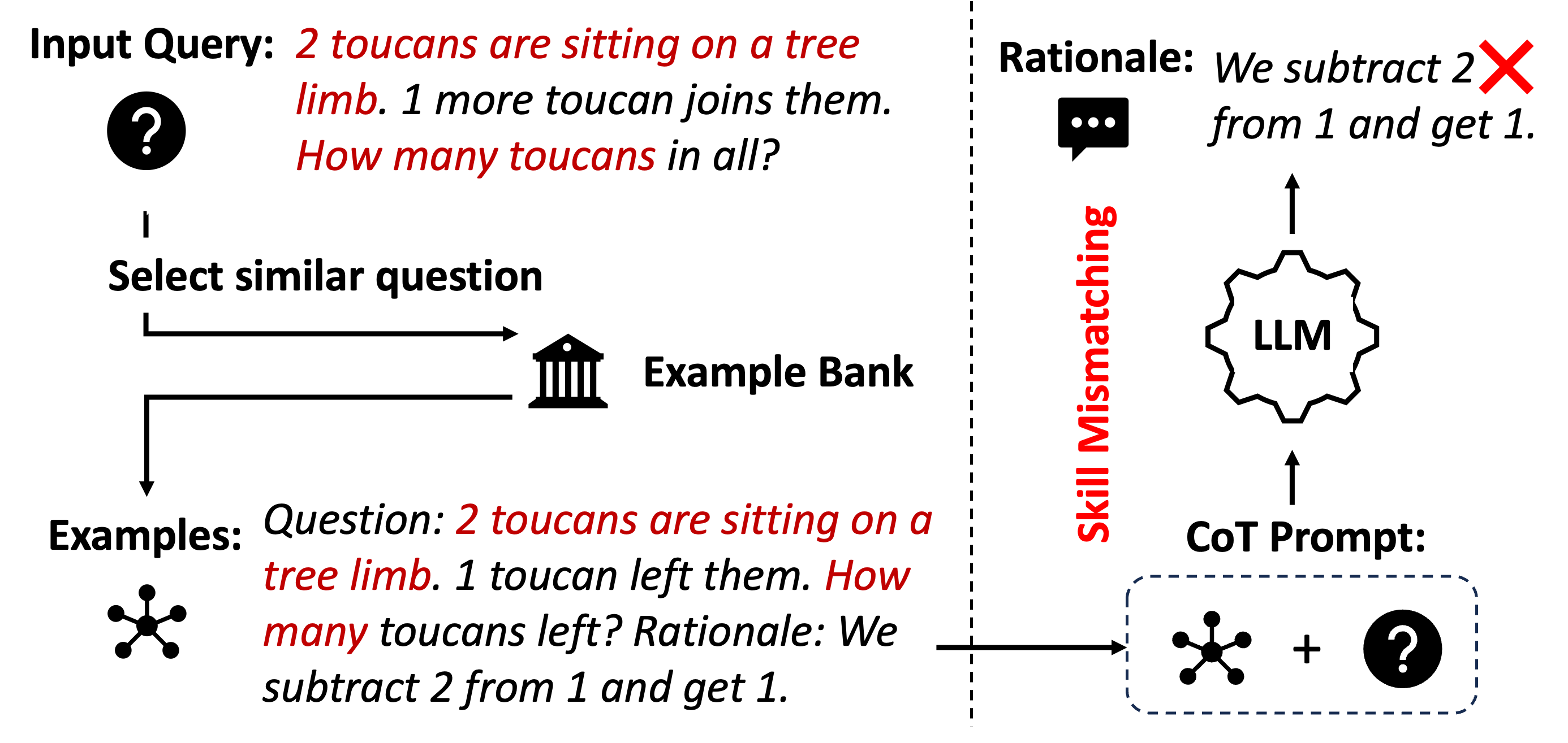</details> (a) Question-similarity-based selection. <details> <summary>extracted/6556870/content/figures/skill_based_selection.png Details</summary>  ### Visual Description ## Flowchart: Problem-Solving Process with LLM ### Overview The flowchart illustrates a structured approach to solving arithmetic word problems using a Large Language Model (LLM). It demonstrates how to abstract a problem into a known skill (e.g., addition), retrieve similar examples, and construct a Chain-of-Thought (CoT) prompt to guide the LLM's reasoning. ### Components/Axes 1. **Input Query**: - Text: "2 toucans are sitting on a tree limb. 1 more toucan joins them. How many toucans in all?" - Symbol: Question mark (?) icon. 2. **Inference Skill**: - Label: "Inference Skill" with a lightbulb icon. 3. **Skill Abstraction**: - Text: "Skill abstraction: addition" (highlighted in blue). 4. **Select Similar Skill**: - Arrows branching to "Example Bank" and "LLM". 5. **Example Bank**: - Icon: Bank building. - Example Question: "Seven red apples and two green apples are in the basket. How many apples are in the basket?" - Rationale: "We add 7 to 2 and get 9." 6. **CoT Prompt**: - Symbol: Question mark (?) combined with example icon. - Text: "Question: ... + ?" (partial view). 7. **LLM with Skill Matching**: - Label: "LLM" inside a gear icon. - Connection: Green arrow labeled "Skill Matching" links to the LLM. ### Detailed Analysis - **Flow Direction**: - The process starts with the Input Query, progresses through Inference Skill and Skill Abstraction, then branches to retrieve examples from the Example Bank or directly engage the LLM via CoT Prompt. - **Text Embedded in Diagrams**: - Example Bank question and rationale are explicitly transcribed. - CoT Prompt combines example structure with the original question. - **Skill Matching**: - Green arrow indicates the LLM's role in aligning the problem with the abstracted skill (addition). ### Key Observations - The flowchart emphasizes **skill abstraction** as a critical step to map word problems to mathematical operations. - The Example Bank provides **structured examples** to guide the LLM's reasoning. - The CoT Prompt merges example patterns with the target problem to scaffold the LLM's response. ### Interpretation This diagram demonstrates a **prompt engineering strategy** for arithmetic problem-solving with LLMs. By abstracting problems into known skills (e.g., addition) and leveraging example-based prompting, the process reduces ambiguity and improves accuracy. The LLM acts as a "reasoning engine" that matches problems to skills and generates step-by-step solutions. The green checkmark on the rationale ("We add 2 to 1 and get 3") visually validates the correctness of the abstracted skill application. 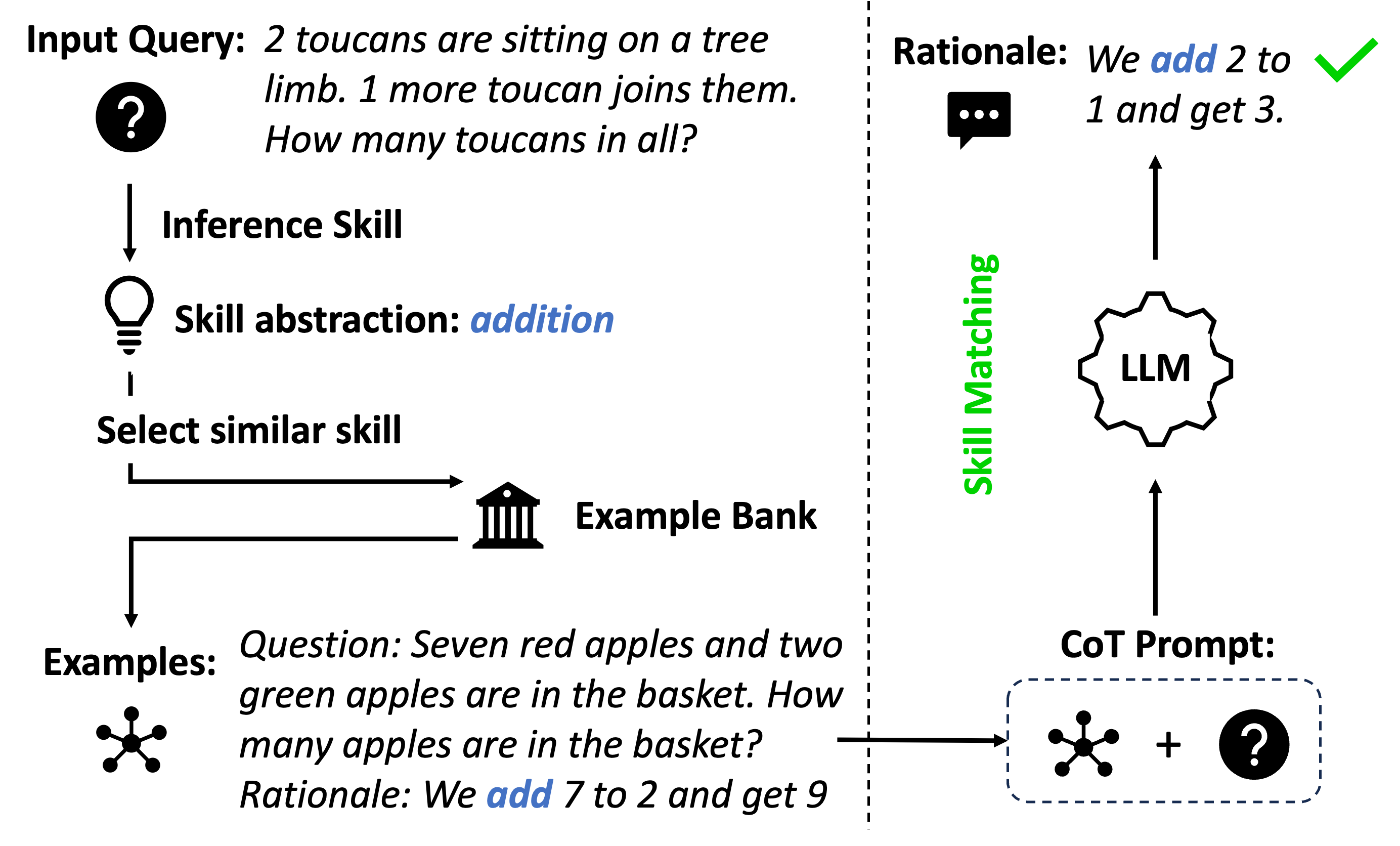</details> (b) Skill-based selection. Figure 1: CoT prompting with examples selected by (a) similar questions and (b) similar skills that (mis)match the skills in their rationales. <details> <summary>extracted/6556870/content/figures/lars.png Details</summary>  ### Visual Description ## Diagram: Technical Architecture for Reasoning-Based Question Answering System ### Overview The diagram illustrates a two-stage technical architecture for processing and answering reasoning-based questions. It combines off-the-shelf embedding models with custom reasoning components, featuring explicit example selection and conditional variational auto-encoder (CVAE) components. The system processes natural language queries through multiple stages of encoding, reasoning, and decoding. ### Components/Axes 1. **Pre-Processing Section (Left Side)** - Input Query Box: Contains sample questions (e.g., "Seven red apples...") - Off-the-Shelf Embedding Model: Standard NLP model for initial text representation - Reasoning Policy: Decision-making component for reasoning strategy - Example Bank: Repository of solved examples (shown with apple/toucan illustrations) - Reasoning Encoder/Decoder: CVAE components for structured reasoning 2. **Selection Section (Right Side)** - Input Query Box: Contains second sample question ("2 toucans...") - Selected Examples Highlight: Visual indicator of retrieved examples - Reasoning Skills Visualization: Circular diagram with colored dots representing reasoning steps - Reasoning Policy: Same component as in pre-processing section - CVAE Components: Mirroring the left section's encoder/decoder structure 3. **Connecting Elements** - Arrows showing data flow between components - Mathematical notation (Q for queries, R for responses, Z for latent representations) - Example Bank icon (classical building symbol) - Reasoning Skills icon (lightbulb) ### Detailed Analysis 1. **Pre-Processing Flow** - Input queries are first processed by an off-the-shelf embedding model - The reasoning policy determines how to handle the query - The system either generates a direct answer (R) or stores it in the example bank - The CVAE components (Reasoning Encoder/Decoder) process the query through latent space (Z) 2. **Selection Mechanism** - New queries trigger example retrieval from the bank - Selected examples are highlighted in red - The reasoning skills visualization shows step-by-step problem decomposition - The same CVAE architecture processes both direct and example-based reasoning 3. **Mathematical Notation** - Q: Represents input queries (e.g., "How many apples...") - R: Denotes system responses (e.g., "We add 7 to 2...") - Z: Latent space representation in the CVAE architecture ### Key Observations 1. The system uses both direct reasoning and example-based reasoning 2. The reasoning policy acts as a central decision-making component 3. The example bank serves as a knowledge repository for similar problems 4. The CVAE architecture enables structured reasoning through latent space manipulation 5. Visual elements (colors, icons) help distinguish different components ### Interpretation This architecture demonstrates a hybrid approach to question answering that combines: 1. **Pre-trained Language Models**: For initial text understanding 2. **Custom Reasoning Components**: For problem-solving logic 3. **Example-Based Learning**: Through the example bank mechanism 4. **Probabilistic Reasoning**: Via the conditional variational auto-encoder The system appears designed to handle arithmetic and simple logical reasoning tasks by: - First determining the appropriate reasoning strategy - Either generating a direct answer or retrieving similar examples - Processing through a structured reasoning pipeline - Maintaining consistency between direct and example-based reasoning paths The use of CVAE suggests the system can handle uncertainty in reasoning steps while maintaining coherent problem-solving trajectories. The explicit example selection mechanism indicates an emphasis on leveraging past solutions for new problems. 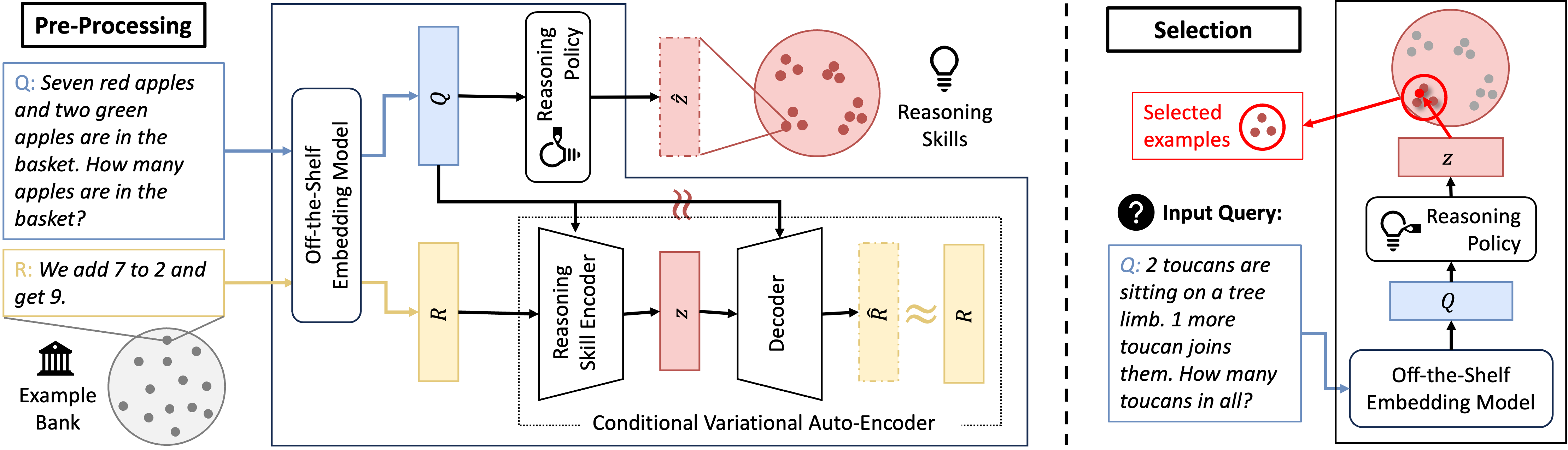</details> Figure 2: An overview of LaRS including a pre-processing stage (left) and a selection stage (right). Reasoning tasks have proven to be particularly difficult for language models and NLP in general Rae et al. (2021); Bommasani et al. (2021); Nye et al. (2021). In the recent literature, chain-of-thought (CoT) prompting, an ICL method, has been proposed to improve LLMs on a wide spectrum of reasoning tasks by guiding LLMs to produce a sequence of intermediate steps (rationale) for generating a (better) final answer Cobbe et al. (2021a); Wei et al. (2022b); Suzgun et al. (2022). The prompts for CoT are composed of demonstrations that contain not only input and output, but also the rationales for why the output holds. The core challenge for ICL lies in designing effective demonstrations to prompt LLMs. Much evidence has indicated the significant impact of demonstrations on the performance of ICL Lu et al. (2021); Liu et al. (2021). To form a prompt, one important setting considers selecting demonstrations from an existing example bank, termed demonstration selection Dong et al. (2022). While a variety of methods exist in the ICL literature for automating this process, CoT prompts are distinct in that they include not only questions and answers but also specially-designed rationales. This distinction highlights the importance of rationales in selecting demonstrations for CoT prompting. Specifically, CoT prompting should select demonstrations that illustrate relevant skills within their rationales to effectively address a given question. For instance, in solving math word problems (as depicted in Fig. 1), a useful rationale involves computing addition to get the correct answer. Selecting few-shot examples based on the question similarity (Fig. 1(a)) might lead to examples showcasing subtraction and generate incorrect rationales. However, skill-based selection (Fig. 1(b)) can align the skills between examples and the given question, which leads to correct answers guided by relevant rationales. To achieve such a skill-based demonstration selection, An et al. (2023b) introduces Skill-KNN, which employs pre-trained LLMs to generate skill descriptions. Then, the few-shot examples are selected based on the embedding of the skill descriptions computed by another pre-trained embedding model. Although this approach is straightforward, the LLM-generated skill descriptions can be somewhat arbitrary, heavily relying on the manually crafted prompts. This reliance constrains its wider applicability across diverse reasoning tasks. Moreover, the approach requires to generate a unique skill description for each example, which limits its scalability to larger example banks. Rather than relying on LLMs, we introduce La tent R easoning S kill Discovery (LaRS), a new skill-based demonstration selection method. This approach learns skills as latent space representations of rationales through unsupervised learning. The essence of LaRS lies in a unique formulation for the generation of rationales, which we term the latent skill model. This model, inspired by the principles of topic models Xie et al. (2021a), conditions the generation of a rationale on both a given question and a latent variable, called a reasoning skill. This latent variable embodies a high-level abstraction of the rationales, such as formats, equations, or knowledge. <details> <summary>extracted/6556870/content/figures/TSNE.png Details</summary>  ### Visual Description ## Scatter Plots: Question Embedding vs LaRS Skill Embedding ### Overview The image contains two side-by-side scatter plots comparing embeddings for reasoning skills. The left plot is labeled "Question Embedding," and the right is labeled "LaRS Skill Embedding." Both plots use colored geometric shapes (circles, triangles, crosses) to represent different reasoning skills, as defined in a legend on the right. ### Components/Axes - **Legend**: - **Black circles**: Compute statistics - **Purple triangles**: Compute rate of change - **Blue crosses**: Compute money cost - **Cyan circles**: Filter tree leaves - **Teal triangles**: Addition/subtraction - **Green circles**: Multiplication - **Teal triangles**: Filter table entries - **Green crosses**: Compute probability - **Yellow circles**: Shortage or surplus? - **Orange triangles**: Reason time schedule - **Red crosses**: Compare numbers - **Red circles**: Others - **Axes**: - No explicit axis labels or scales are visible. - X and Y axes are unlabeled, but data points are distributed across the plot area. ### Detailed Analysis #### Question Embedding (Left Plot) - **Compute statistics** (black circles): Clustered in the top-right quadrant. - **Compute rate of change** (purple triangles): Scattered in the middle-left. - **Compute money cost** (blue crosses): Spread across the middle-right. - **Filter tree leaves** (cyan circles): Concentrated in the bottom-left. - **Addition/subtraction** (teal triangles): Clustered in the top-center. - **Multiplication** (green circles): Scattered in the middle-right. - **Filter table entries** (teal triangles): Overlapping with "Addition/subtraction" in the top-center. - **Compute probability** (green crosses): Located in the bottom-right. - **Shortage or surplus?** (yellow circles): Clustered in the bottom-left. - **Reason time schedule** (orange triangles): Spread across the bottom-center. - **Compare numbers** (red crosses): Scattered in the top-left. - **Others** (red circles): Concentrated in the bottom-left. #### LaRS Skill Embedding (Right Plot) - **Compute statistics** (black circles): Clustered in the top-right. - **Compute rate of change** (purple triangles): Scattered in the middle-left. - **Compute money cost** (blue crosses): Spread across the middle-right. - **Filter tree leaves** (cyan circles): Concentrated in the bottom-left. - **Addition/subtraction** (teal triangles): Clustered in the top-center. - **Multiplication** (green circles): Scattered in the middle-right. - **Filter table entries** (teal triangles): Overlapping with "Addition/subtraction" in the top-center. - **Compute probability** (green crosses): Located in the bottom-right. - **Shortage or surplus?** (yellow circles): Clustered in the bottom-left. - **Reason time schedule** (orange triangles): Spread across the bottom-center. - **Compare numbers** (red crosses): Scattered in the top-left. - **Others** (red circles): Concentrated in the bottom-left. ### Key Observations 1. **Consistent Clustering**: Skills like "Compute statistics" (black circles) and "Others" (red circles) occupy similar positions in both plots, suggesting stable embeddings across methods. 2. **Overlap**: Some skills (e.g., "Addition/subtraction" and "Filter table entries") share regions in both plots, indicating potential semantic similarity. 3. **Anomalies**: "Compute probability" (green crosses) appears in the bottom-right in both plots, which may reflect lower frequency or distinctiveness in the dataset. 4. **Spatial Patterns**: Skills like "Shortage or surplus?" (yellow circles) and "Reason time schedule" (orange triangles) are consistently in the bottom-left, possibly indicating lower importance or less frequent occurrence. ### Interpretation The embeddings effectively group similar reasoning skills, as evidenced by overlapping clusters in both plots. The consistent placement of "Others" (red circles) in the bottom-left suggests these skills are less distinct or less frequently represented in the data. The separation of "Compute statistics" (top-right) and "Filter tree leaves" (bottom-left) highlights differences in how these skills are encoded. The LaRS Skill Embedding plot mirrors the Question Embedding plot, implying that both methods capture similar semantic relationships. However, minor variations (e.g., "Compute probability" in the bottom-right) may reflect methodological differences in embedding generation. This visualization underscores the importance of embedding techniques in preserving skill relationships for applications like adaptive learning systems or skill-based assessments. 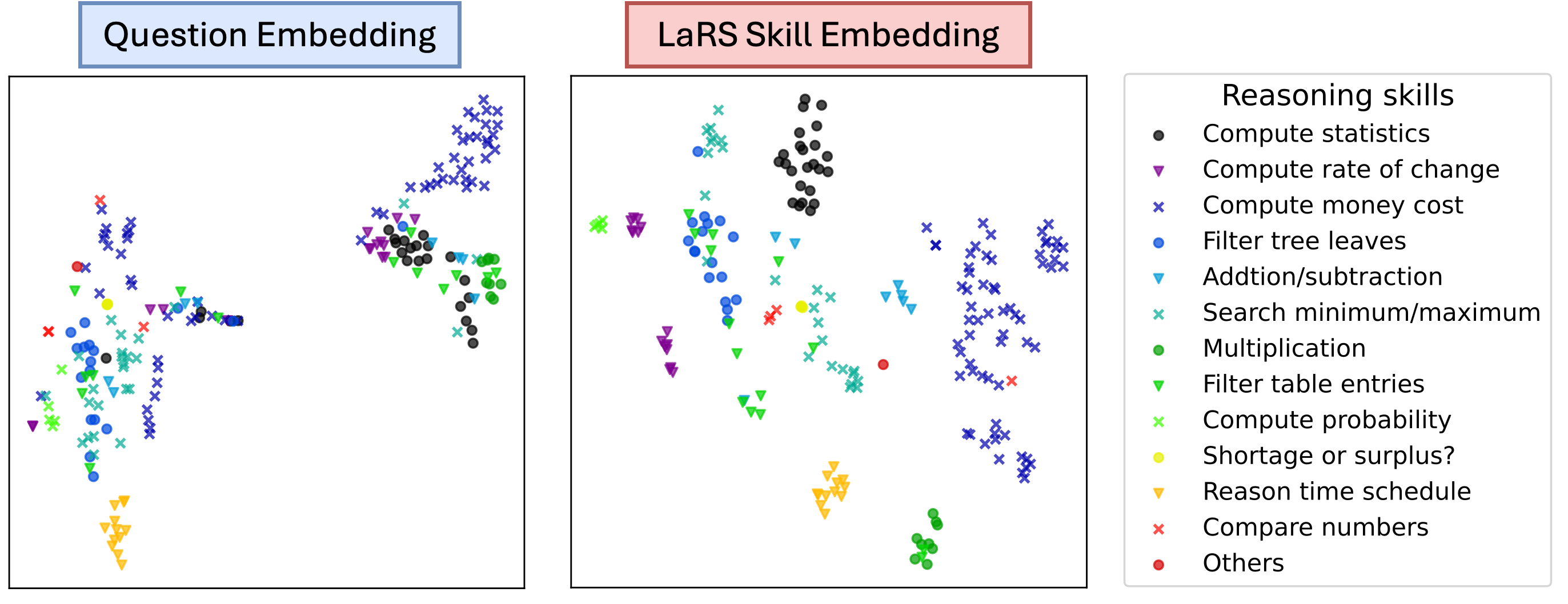</details> Figure 3: t-SNE projections of question embedding and LaRS reasoning skill embedding of the exmaples from TabMWP Lu et al. (2022) dataset. The 12 different colors correspond to 12 skill labels annotated by human. Under the skill model formulation, LaRS utilizes a Conditional Variational Auto-encoder (CVAE) to approximate the generation of rationales on a small dataset from the example bank. As a result, two probabilistic models can be learned concurrently: (1) a reasoning skill encoder that maps an example to the actual reasoning skills demonstrated in the rationale; and (2) a reasoning policy that predicts the reasoning skills required for a particular question. This method of learning through a CVAE, especially when applied to a small dataset from the example bank, is both cost-efficient and fast compared to Skill-KNN. Fig. 2 presents an overview of LaRS. In addition, Figure 3 shows the learned reasoning skill embedding (right) that effectively separates examples with different skill labels, while the off-the-shelf question embedding does not. The efficacy of LaRS is evaluated on four different benchmarks based on five backbone LLMs with varying scales. The method is also compared with baseline approaches, including an oracle method that assumes access to ground truth rationales. LaRS consistently outperforms Skill-KNN and also matches the oracle performance in almost half of the experiments. In addition, LaRS reduces half of the LLM inference, eliminates the need of human prompt design, and maintains better robustness to sub-optimal example banks. A summary of this paper’s contribution is as follows: - We propose LaRS, a novel unsupervised demonstration selection approach for CoT prompting, and empirically verify its effectiveness through large scale experiments. - We introduce the latent skill model, a plausible formulation for CoT reasoning, which has illuminated a deeper understanding of CoT prompting. - We present theoretical analyses of the optimality of the latent-skill-based selection method. <details> <summary>extracted/6556870/content/figures/causal_graph.png Details</summary>  ### Visual Description ## Diagram: Comparative Analysis of Zero-shot/human, Zero-shot CoT, and Few-shot CoT Methods ### Overview The image presents three side-by-side diagrams comparing three reasoning methods: **Zero-shot/human**, **Zero-shot Chain-of-Thought (CoT)**, and **Few-shot CoT**. Each diagram illustrates the flow of information between three core components: **Q** (query), **R** (response), and **z** (context/knowledge). Arrows represent directional relationships, with labels indicating specific processes or inputs. --- ### Components/Axes 1. **Nodes**: - **Q**: Blue circle (query/input). - **R**: Yellow circle (response/output). - **z**: Pink circle (context/knowledge base). 2. **Arrows**: - **Zero-shot/human**: - Dashed arrow from **z** → **Q** (context influences query). - Solid arrow from **Q** → **R** (direct query-to-response mapping). - **Zero-shot CoT**: - Single arrow from **z** → **R** labeled **(prefix, Q)** (context + query prefix guides response). - **Few-shot CoT**: - Single arrow from **z** → **R** labeled **(Q₁, R₁, ..., Qₖ, Rₖ, Q)** (sequence of query-response pairs + final query). 3. **Color Coding**: - Blue (**Q**), Pink (**z**), Yellow (**R**) are consistent across diagrams but lack a formal legend. --- ### Detailed Analysis #### Zero-shot/human - **Flow**: Context (**z**) indirectly shapes the query (**Q**), which directly determines the response (**R**). - **Key Feature**: Human-like reasoning where context is preprocessed into the query before response generation. #### Zero-shot CoT - **Flow**: Context (**z**) directly influences the response (**R**) via a **prefix** combined with the query (**Q**). - **Key Feature**: Explicit use of a prefix (e.g., "Let's think step by step") to guide reasoning without intermediate query refinement. #### Few-shot CoT - **Flow**: Context (**z**) incorporates a **sequence of query-response pairs** (Q₁→R₁, ..., Qₖ→Rₖ) alongside the final query (**Q**) to generate **R**. - **Key Feature**: Leverages multiple examples to condition the response, mimicking few-shot learning in NLP. --- ### Key Observations 1. **Zero-shot/human** relies on indirect context integration, while **CoT methods** directly embed context into the response process. 2. **Few-shot CoT** introduces complexity by requiring multiple example pairs, suggesting scalability challenges. 3. All methods share the same core components (**Q**, **R**, **z**), but differ in how **z** is utilized. --- ### Interpretation This diagram highlights evolutionary steps in reasoning methods: - **Zero-shot/human** represents baseline human-like reasoning. - **Zero-shot CoT** introduces explicit reasoning guidance via prefixes. - **Few-shot CoT** advances further by incorporating example-driven context, aligning with modern few-shot learning paradigms in AI. The absence of numerical data suggests this is a conceptual comparison rather than an empirical study. The progression from dashed to sequential arrows implies increasing complexity and potential performance gains at the cost of computational overhead. 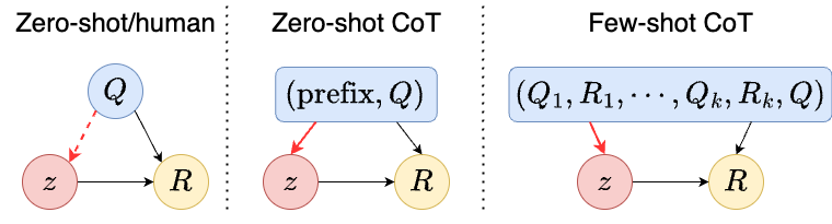</details> Figure 4: Causal graphs for prompting with zero-shot/human (left), zero-shot CoT (middle), and few-shot CoT (right) for generating rationales via skills. The dashed arrow from $Q$ to $z$ indicates possible sub-optimal inference of the reasoning skills from both human and zero-shot LLM generations. ## 2 Related Work ### 2.1 CoT Reasoning CoT prompting is a special prompt design technique that encourages LLMs to generate intermediate rationales that guide them towards providing accurate final answers. These rationales can exhibit remarkable flexibility in their styles. For instance, the original work by Wei et al. (2022b) specially designs rationales in the in-context demonstrations to suit different reasoning tasks. Moreover, novel prompt designs that highlight diverse formats of the rationales have emerged to enhance CoT prompting. For example, Kojima et al. (2022) proposed Program of Thoughts (PoT) that disentangles textual reasoning from computation, with the latter specially handled through program generation. In contrast to manual design, our method LaRS can be thought of as automatic discovery of diverse rationale styles from an example bank. This method can also dynamically select reasoning skills based on the specific questions. Worth noting, Chen et al. (2023) introduces SKills-in-Context (SKiC), which confines rationale generation to predefined “skills” within the prompt. Although sharing a similar motivation to LaRS, we emphasize two crucial distinctions: (1) while SKiC relies on manual “skills” design, LaRS automatically discovers them, (2) SKiC presents a full list of “skills” in the prompt, allowing LLMs to select from them, whereas LaRS learns the skill selection from the example bank, explicitly instructing LLMs on which skill to employ through in-context examples. ### 2.2 Demonstration Selection Demonstration selection refers to a special setting, where the prompts are constructed by selecting examples from an example bank. In this context, our LaRS aligns with the paradigm of unsupervised demonstration selection, which involves designing heuristics for this selection process. A variety of heuristics have been explored, including similarity Gao et al. (2021); Hu et al. (2022), diversity Zhang et al. (2022), coverage Gupta et al. (2023), and uncertainty Diao et al. (2023). Among these, Skill-KNN (An et al. (2023b)) shares the closest resemblance to our approach. However, Skill-KNN relies on pre-trained LLMs to provide “skill” annotations, which could be arbitrary and resource-intensive, requiring extensive inferences of LLMs and human prompt design. In contrast, LaRS automatically discovers reasoning skills by learning a lightweight CVAE represented by two-layer MLPs and standard loss function. In addition, the selections based on these discovered reasoning skills are theoretically-grounded based on the latent skill model and the theoretical analyses presented in this paper. ## 3 Formulation In this section, we formally describe the skill model, a new formulation for explaining the generation of rationales in CoT reasoning. In Section 3.1, the skill model is first introduced to describe the human-generated rationales. Then, Section 3.2 illustrates how the skill model can be adapted to LLM-generated rationales. Finally, leveraging the concept of reasoning skill as outlined in the skill model, a new latent-skill-based demonstration selection method is formally described in Section 3.3. ### 3.1 Skill Model Let $\mathcal{X}$ be the set of all sequences of tokens, $\mathcal{Z}$ be the continuous vector space of latent reasoning skills, and $P_{H}$ denotes the probability distribution of real-world natural language. CoT reasoning is to generate a rationale $R\in\mathcal{X}$ given a question $Q\in\mathcal{X}$ , whose correctness For math word problems, whose answers are discrete labels, the correct rationale should contain the correct answer label as the final step. For code generation, the correct rationale should be the correct code. can be verified by an indicator function $\mathbb{1}(R,Q):=\mathbb{1}(R\text{ is the correct rationale for }Q)$ . The skill model assumes that the real-world conditional distribution of $R$ given $Q$ can be described as follows: where, $P_{H}(z\mid Q)$ is the posterior of selecting latent reasoning skills in human reasoning, called a reasoning policy. $P_{H}(R\mid z,Q)$ is the posterior distribution of generating $R$ given a question $Q$ and a reasoning skill $z$ . A causal graph illustrating such a generation process involving a latent reasoning skill $z$ is presented in Fig. 4 on the left. Unlike Wang et al. (2023), this formulation considers a dependency of $z$ on $Q$ reflecting a preference for selecting particular reasoning skills to solve a given question. We justify this formulation as follows: 1. Rationales can exhibit remarkable flexibility, manifesting diverse formats, topics, and knowledge, which can naturally be abstracted into the high-level concepts of reasoning skills. 1. The selection of these skills is not bound by strict determinism. For instance, diverse reasoning paths and formats could all contribute toward finding the correct final answer. Therefore, real-world data is a mixture of diverse skills captured by a stochastic reasoning policy $P_{H}(z\mid Q)$ . ### 3.2 CoT prompting LLMs are pre-trained conditional generators. Given an input query $X\in\mathcal{X}$ , the conditional distribution of an output $Y\in\mathcal{X}$ generated by LLMs can be written as $P_{M}(Y\mid X)$ . LLMs are usually trained on generic real-world data distribution such that $P_{M}(Y\mid X)\approx P_{H}(Y\mid X)$ . Prior studies have presented an implicit topic model formulation in explaining the in-context learning mechanisms of LLMs Wang et al. (2023); Xie et al. (2021a). Similarly, we posit that LLMs can be viewed as implicit skill models for generating rationales. To elaborate, when generating rationales, LLMs’ conditional distribution $P_{M}(R\mid Q)$ can be extended as follows (with illustrations in Fig. 4 on the left): This implicit skill model assumes that LLMs also infer reasoning skills $z$ , which resembles the real-world generation of rationales. The above formulation only encompasses the zero-shot generation of rationales. In practice, prompts are commonly provided to guide LLMs’ generation. In general, two CoT prompting strategies exist: zero-shot CoT, employing a prompt comprising a short prefix and a test question, and few-shot CoT, employing a prompt containing pairs of questions and rationales. Denoting $pt\in\mathcal{X}$ as a prompt, a unified formulation for both prompting strategies can be derived as follows: 0-shot CoT: $pt=(\text{prefix},Q)\text{ or }(Q,\text{prefix})$ $k$ -shot CoT: $pt=(Q_{1},R_{1},\cdots,Q_{k},R_{k},Q)$ Here, the formulation is simplified such that the use of prompts only influences the probability distribution of $z$ . For instance, a prefix specifying the generation’s format can be interpreted as specifying the reasoning skill $z$ by shaping the distribution from $P_{M}(z\mid Q)$ to $P_{M}(z\mid pt)$ . This simplification aligns with empirical evidence suggesting that in-context examples serve as mere pointers to retrieve already-learned knowledge within LLMs Shin et al. (2020); Min et al. (2022); Wang et al. (2022). Drawing upon this formulation, we can gain insight into the failure of zero-shot generation. In general, real-world data is inherently noisy, indicating that the reasoning policy $P_{H}(z\mid Q)$ may be sub-optimal, and the reasoning skills are not chosen to maximize the accuracy of answering a test question. Trained on this generic real-world data distribution, $P_{M}(z\mid Q)$ could also be sub-optimal, leading to the failure of zero-shot generation. On the other hand, CoT prompting improves the reasoning performance by shaping the distribution of reasoning skills using carefully-designed prompts that contain either prefix or few-shot examples. ### 3.3 Skill-Based Demonstration Selection The analysis above suggests that the key to the success of CoT prompting is to design an effective prompt that improve upon the posterior distribution of human’s preference of reasoning skills $P_{H}(z\mid Q)$ . To design an effective prompt, the demonstration selection problem assumes access to an example bank of question-rationale pairs, denoted as $\mathcal{D}_{E}=\{(R,Q)\}$ . This example bank is usually specially-crafted and has a distribution different from the real-world distribution. Denoting $P_{E}$ as the distribution of the example bank, $R$ is distributed according to $P_{E}(R\mid Q)$ for all $(R,Q)\in\mathcal{D}_{E}$ . Given $\mathcal{D}_{E}$ , the demonstration selection is to select a few question-rationale pairs from $\mathcal{D}_{E}$ . Assuming that each selected demonstration is i.i.d, a demonstration selection method can be uniquely defined as a probabilistic model $g(Q,R|Q_{\text{test}}):=\mathcal{X}\mapsto\Delta(\mathcal{X})$ that maps a test question $Q_{\text{test}}$ to a probability distribution of demonstrations. Then, we can formally define the skill-based demonstration selection method as follows: **Definition 1** *Skill-based demonstration selection is given by* Intuitively, this selection method maximizes the probability of a selected demonstration showcasing the reasoning skill that is likely to be chosen according to $P_{E}(z\mid Q)$ . Since the example bank is usually specially-crafted and contains rationales showcasing “better” reasoning skills, the in-context examples that align with $P_{E}(z\mid Q)$ are intuitively more effective. In Section 4.3, we provide theoretical analysis of the optimality of this skill-based selection when conditioned on certain ideal assumptions of the example bank and LLMs. ## 4 Method To enable the skill-based demonstration selection (Definition 1), we introduce our approach LaRS , which involves learning a conditional variational autoencoder (CVAE) to approximate $P_{E}$ using the data from the example bank $\mathcal{D}_{E}$ . We then outline a practical demonstration selection process aligning with the skill-based selection. The schematic overview of LaRS (right) and the corresponding demonstration selection process (left) are illustrated in Figure 2. ### 4.1 Latent Reasoning Skill Discovery The conditional variational autoencoder (CVAE) has emerged as a popular approach for modeling probabilistic conditional generation. As one specific case, the skill model, introduced in this paper, can effectively be represented as a CVAE. Therefore, we introduce LaRS that employs a CVAE to approximate the generation of rationales using the data from the example bank $\mathcal{D}_{E}=\{(Q,R)\}$ . In particular, this CVAE includes three coupled models: an encoder model, a decoder model, and a reasoning policy model, independently parameterized by $\omega$ , $\psi$ , and $\phi$ respectively. Drawing from the notations introduced in the skill model, the reasoning policy model is a conditional Bayesian network $\pi_{\phi}(z\mid Q)$ , determining the posterior distribution of latent reasoning skill $z$ given a question $Q$ . The decoder model is also a conditional Bayesian network $p_{\psi}(R\mid z,Q)$ that generates a rationale $R$ , conditioned on both $Q$ and $z$ , where $z$ is sampled from $\pi_{\phi}(z\mid Q)$ . Finally, the encoder model $q_{\omega}(z\mid Q,R)$ is another conditional Bayesian network, mapping a question-rationale pair to $z$ . In this paper, we train this CVAE using classical variational expectation maximization and the reparameterization trick. Specifically, the classical variational expectation maximization optimizes a loss function as follows: $\displaystyle\mathcal{L}_{\text{CVAE}}(\phi,\omega,\psi)=\mathcal{L}_{\text{ recon}}+\mathcal{L}_{\text{KL}}$ (4) $\displaystyle\mathcal{L}_{\text{recon}}=-\mathbb{E}_{(Q,R)\sim\mathcal{D}_{E}, z\sim q_{\omega}(\mid Q,R)}[\log p_{\psi}(R|z,Q)]$ $\displaystyle\mathcal{L}_{\text{KL}}=~{}\mathbb{E}_{(Q,R)\sim\mathcal{D}_{E}}[ \text{D}_{\text{KL}}(q_{\omega}(z\mid Q,R)\parallel\pi_{\phi}(z\mid Q))]$ By training to minimize this loss function, $q_{\omega}$ and $\pi_{\phi}$ can be learned to effectively approximate the conditional distributions $P_{E}(z\mid Q,R)$ and $P_{E}(z\mid Q)$ . It is worth noting that the decoder model acts an auxiliary model that only roughly reconstructs rationales for the purpose of training the encoder and the reasoning policy model, and is not deployed to generate rationales in the downstream tasks. Ideally, all three models would be represented by language models, processing token sequences as input and generating token sequences as output. However, training full language models for demonstration selections can be computationally expensive. Instead, we adopt a pre-trained embedding model denoted as $f:\mathcal{X}\mapsto\Theta$ , which maps the token space $\mathcal{X}$ to an embedding space $\Theta$ . Consequently, the decoder model, encoder model, and reasoning policy model transform into $p_{\psi}(f(R)|z,f(Q))$ , $q_{\omega}(z|f(Q,R))$ , and $\pi_{\phi}(z|f(Q))$ , respectively. They now condition on and generate the embeddings instead of the original tokens. In the actual implementation, we use the same feed-forward neural network to represent both $\pi_{\phi}$ and $q_{\omega}$ , predicting the mean and variance of Gaussian distributions of latent reasoning skills. On the other hand, $p_{\psi}$ is a feed-forward neural network that deterministically predicts a value in the embedding space. ### 4.2 Demonstration Selection Since the distribution $P_{E}(Q,R\mid z)$ in Definition 1 is practically intractable, we propose a selection process that effectively aligns with the skill-based selection using the learned $\pi_{\phi}$ and $q_{\omega}$ . For a given test question $Q_{\text{test}}$ , the desirable reasoning skill $z_{\text{test}}=\operatorname*{arg\,max}_{z}[\pi_{\phi}(z|f(Q_{\text{test}}))]$ can be computed using the reasoning policy. Subsequently, each example from the example bank can be scored based on the cosine similarity between $z_{\text{test}}$ and $z_{\text{post}}$ , where $z_{\text{post}}=\operatorname*{arg\,max}_{z}[q_{\omega}(z|Q,R))]$ represents the maximum likelihood skill of the current example. Finally, a CoT prompt can be constructed by selecting the top- $k$ examples according to the computed scores. The step-by-step procedure is outlined in Algorithm 1. ### 4.3 Theoretical Analysis In this section, we provide a theoretical analysis of the optimality of the skill-based selection by Definition 1. Let $P_{M}(R\mid Q,g)$ denotes LLMs’ conditional distribution of a rationale $R$ given a test question $Q$ under a demonstration selection method $g$ . $P_{M}(R\mid Q,g)$ can be extended as follows: $\displaystyle P_{M}(R\mid Q,g)$ $\displaystyle=\int_{\mathcal{X}^{k}}P_{M}(R\mid pt)\Pi_{i=1}^{k}[g(Q_{i},R_{i} \mid Q)d(Q_{i},R_{i})]$ Here, each demonstrations $(Q_{i},R_{i})$ is independently sampled from $g(Q_{i},R_{i}\mid Q),\forall i=1,\cdots,k$ . These $k$ demonstrations form a prompt $pt=(Q_{1},R_{1},\cdots,Q_{k},R_{k},Q)$ . We want to show that $P_{M}(R\mid Q,g)$ is the optimal conditional distribution that maximizes the accuracy of rationales if the selection follows skill-based selection method or $g=g_{skill}$ . We begin by defining the optimal conditional distribution as follows: **Definition 2** *Optimal conditional distribution of rationales given questions $P^{*}(R\mid Q)$ is given by: $P^{*}(R\mid Q)=\operatorname*{arg\,max}_{P(\cdot\mid Q)\in\Delta(\mathcal{X})} \int_{\mathcal{X}}\mathbb{1}(R,Q)P(R\mid Q)dR$ Here $\mathbb{1}(R,Q)$ is the indicator function of the correctness of $R$ given a question $Q$ (see Section 3.1).* Then, we state two major assumptions as follows: **Assumption 1** *Example bank is sampled from the optimal conditional distribution, or $P_{E}(R\mid Q)=P^{*}(R\mid Q)$ .* **Assumption 2** *Humans and LLMs are expert rationale generators given reasoning skills and questions, meaning that $P_{H}(R\mid z,Q)=P_{E}(R\mid z,Q)=P_{M}(R\mid z,Q)$ .* Assumption 1 is rooted in the fact that example banks are human-crafted that contains the most useful rationales for answering the questions. In Assumption 2, $P_{M}$ capturing $P_{H}$ is a common assumption in the literature studying LLMs Xie et al. (2021b); Saunshi et al. (2020); Wei et al. (2021). $P_{E}(R\mid z,Q)=P_{H}(R\mid z,Q)$ is based on the assumption that reasoning skills are shared across humans, and the generation of rationales is identical given the same reasoning skills and questions. Based on the above definiton and two assumptions, we prove the following theorem. **Theorem 1** *A LLM gives the optimal conditional distribution of rationales given questions: $$ P_{M}(R\mid Q,g_{skill})=P^{*}(R\mid Q) $$ If (1) it is prompted by $k\rightarrow\infty$ in-context examples selected by the skill-based selection $g_{skill}$ defined by Definition 1, (2) Assumption 2 and Assumption 1 hold.* Appendix E presents the proof for Theorem 1. ## 5 Experiments This section describes the experimental settings, baselines, metrics, and main results. ### 5.1 Dataset For benchmarking, the selection methods are evaluated on four challenging datasets, including two datasets of Math Word Problem (MWP): TabMWP, GSM8K, one text-to-SQL dataset: Spider, and one semantic parsing dataset: COGS. Each dataset is split into a training set used to learn LaRS models and a test set used to evaluate the selection methods. While the training sets may potentially be large, we use randomly sampled 1K examples from the training set as the example bank, from which, the examples can be selected for CoT prompting. Detailed descriptions of the datasets and splitting are presented in Appendix B. To measure the performances, we use the answer accuracy for TabMWP and GSM8K, with the answers extracted by searching the texts right after a prefix The answer is. For Spider, we use the official execution-with-values accuracy We use the official evaluation scripts for Spider in https://github.com/taoyds/test-suite-sql-eval.. For COGS, we report the exact-match accuracy for semantic parsing. ### 5.2 Selection Methods Our method LaRS is compared with the following four baselines. All the hyper-parameters related to these methods are listed in Appendix B. #### Skill-KNN This baseline represents a state-of-the-art (SOTA) skill-based selection method. It employs pre-trained LLMs to generate skill descriptions for both the questions in the example bank and the test question. Then, the method selects examples whose skill descriptions most closely match that of the test question to form the prompt, using cosine similarity computed with a pre-trained embedding model. To examine the dependency on the LLMs’ ability to generate skill descriptions, we introduce two variations: Skill-KNN-large, which uses the larger LLM gpt-3.5-turbo, and Skill-KNN-small, which uses the smaller LLM Falcon-40B-instruct. Additionally, to evaluate the effect of human-annotated skill descriptions prompting the LLMs to generate new skills, we introduce Skill-KNN-zero, which uses gpt-3.5-turbo to generate skill descriptions in a zero-shot fashion. Skill-KNN-zero closely resembles the setting of LaRS , as it does not rely on human prompt design. Therefore, LaRS is primarily compared with Skill-KNN-zero. #### Random This baseline randomly selects $k$ in-context examples from the example bank. For each test question, the accuracy is reported as an average over three independent random selections. #### Retrieval-Q This baseline employs a pre-trained embedding model to encode a test question, and selects in-context examples based on the cosine similarity between embeddings from examples’ questions and the test question. #### Retrieval-R (oracle) This baseline employs a pre-trained embedding model to encode the ground-truth rationale of a test question, and selects in-context examples based on the cosine similarity between examples’ rationales and the ground-truth rationale. ### 5.3 Backbones and Hyper-parameters In terms of the backbone models, the ICL is conducted by two OpenAI language models: gpt-4o and gpt-3.5-turbo, two Anthropic model: claude-3-sonnet and claude-3-haiku, and one smaller-scale Falcon-40B-Instruct Xu et al. (2023). All the embedding is computed by a pre-trained embedding model, Deberta-v2-xlarge He et al. (2021). We also investigate different choices of embedding model in Section C. During inference, the temperature is set to 0 (i.e., greedy decoding) to reduce the variance. The CoT prompts contain $k=2,4,4,8$ in-context examples for TabMWP, GSM8K, Spider, and COGS, respectively. ### 5.4 Performance comparison results Table 7 presents experiment result summary. Detailed descriptions are as follows: | Method Backbone: gpt-3.5-turbo Random | TabMWP 62.4 +0.0 | GSM8K 75.7 +0.0 | Spider 46.8 +0.0 | COGS 67.5 +0.0 | | --- | --- | --- | --- | --- | | Retrieval-Q | 72.3 +9.9 | 75.6 –0.1 | 49.9 +3.1 | 88.5 +21.0 | | Skill-KNN-zero | 77.7 +15.3 | 75.0 –0.7 | 49.0 +2.2 | 77.9 +10.8 | | LaRS (ours) | 78.1 +15.7 | 76.8 +1.1 | 53.0 +6.2 | 94.8 +27.2 | | Retrieval-R (oracle) | 77.4 +15.0 | 75.5 –0.2 | 64.4 +17.6 | 95.7 +28.2 | | Backbone: gpt-4o | | | | | | Random | 87.6 +0.0 | 78.1 +0.0 | 74.1 +0.0 | 73.0 +0.0 | | Retrieval-Q | 85.9 –1.7 | 78.1 +0.0 | 75.9 +1.8 | 86.9 +16.9 | | Skill-KNN-zero | 87.7 +0.1 | 78.6 –0.5 | 76.6 +2.5 | 78.1 +5.1 | | LaRS (ours) | 87.9 +0.3 | 78.3 +0.2 | 77.2 +3.1 | 90.2 +17.2 | | Retrieval-R (oracle) | 88.8 +1.2 | 77.1 –1.0 | 78.1 +4.0 | 92.8 +19.8 | | Backbone: claude-3-sonnet | | | | | | Random | 92.6 +0.0 | 93.3 +0.0 | 61.7 +0.0 | 79.2 +0.0 | | Retrieval-Q | 93.1 +0.5 | 92.4 –0.9 | 61.8 +0.1 | 94.6 +15.4 | | Skill-KNN-zero | 93.1 +0.5 | 92.1 –1.2 | 61.9 +0.2 | 86.6 +7.4 | | LaRS (ours) | 93.7 +1.1 | 93.6 +0.3 | 62.2 +0.5 | 96.9 +17.7 | | Retrieval-R (oracle) | 94.1 +1.5 | 92.8 –0.5 | 62.4 +0.7 | 97.6 +18.4 | | Backbone: claude-3-haiku | | | | | | Random | 88.6 +0.0 | 88.6 +0.0 | 60.2 +0.0 | 66.2 +0.0 | | Retrieval-Q | 92.2 +3.6 | 88.6 +0.0 | 60.0 –0.2 | 88.5 +22.3 | | Skill-KNN-zero | 93.3 +4.7 | 88.8 +0.2 | 61.0 +0.8 | 79.7 +13.5 | | LaRS (ours) | 93.3 +4.7 | 87.6 –1.0 | 61.3 +1.1 | 89.9 +23.7 | | Retrieval-R (oracle) | 92.4 +3.8 | 88.9 +0.3 | 61.2 +1.0 | 96.5 +30.3 | | Backbone: Falcon-40B-Instruct | | | | | | Random | 45.7 +0.0 | 38.8 +0.0 | 20.6 +0.0 | 45.1 +0.0 | | Retrieval-Q | 51.9 +6.2 | 37.3 –1.5 | 22.1 +1.5 | 73.9 +28.8 | | Skill-KNN-small | 51.4 +5.7 | 36.5 –2.3 | 20.3 –0.3 | 59.4 +14.3 | | Skill-KNN-zero | 55.2 +9.5 | 38.7 –0.1 | 23.3 +2.7 | 82.1 +37.0 | | LaRS (ours) | 57.7 +12.0 | 39.1 +0.3 | 24.8 +4.2 | 89.5 +44.4 | | Retrieval-R (oracle) | 61.2 +15.5 | 40.4 +1.6 | 39.9 +19.3 | 90.3 +45.2 | Table 1: Main results (%) across all backbone models and datasets. Numbers in bold represent the best results for each backbone model across all selection methods. The subscripted gray values indicate the relative improvement over Random selection. #### LaRS matches SOTA skill-based selection methods with superior computational efficiency. As shown in Table 7, across all four benchmarks and five backbone models tested, LaRS outperforms Skill-KNN-zero in 18 out of 20 experiments. This result highlights the effectiveness of the latent reasoning skills learned through unsupervised learning with small CVAE models, achieving comparable performance to the skill descriptions crafted by extensively pre-trained LLMs. Notably, Skill-KNN-zero uses the powerful LLM gpt-3.5-turbo for skill generations. However, in scenarios where only less capable LLMs are available, such as lacking an internet connection and requiring local inference, Skill-KNN-small, which uses the less capable LLM Falcon-40B-instruct, suffers significant performance drops across all four benchmarks. In contrast, LaRS does not require powerful LLMs and achieves similar performance boosts for smaller backbone models like Falcon-40B-Instruct compared to Skill-KNN-zero. Furthermore, in Table 3, we present a comparison of computational overhead, including computing time, estimated cost for pre-processing the example bank, and cost for each input query during selection, among Retrieval-Q, LaRS, Skill-KNN-zero, and a supervised selection method PromptPG Lu et al. (2022). Our method achieves accuracy comparable to Skill-KNN-zero, requiring no LLM inferences (approximately $30 savings per 1k examples) and reducing computing time by 1.5 hours per 1k examples during pre-processing, along with more than 100% less cost per input query. Detailed experimental settings for estimating these costs can be found in Appendix B. #### LaRS is more robust to sub-optimal example banks. Skill-KNN selects examples based solely on the questions. For example, it selects examples whose questions require the same skills as the given question. However, sub-optimal example banks may include examples with incorrect or sub-optimal rationales, which should be avoided. In contrast, LaRS considers both questions and rationales when computing the reasoning skill embedding, enhancing its robustness to sub-optimality. Table 2 presents the answer accuracy of Skill-KNN-zero and LaRS on the TabMWP and COGS benchmark with sub-optimal example banks, where 10%, 20% and 30% of rationales are replaced by random rationales from the same example banks. Skill-KNN-zero suffers from a 3% and 11.7% performance drop at the replacement rate of 30%, while LaRS experiences only a 0.1% and 1.9% performance drop under the same conditions. | Skill-KNN-zero LaRS Benchmark | 77.7 78.1 COGS | 77.0 –0.9% 78.1 –0.0% | 76.2 –1.9% 78.0 –0.1% | 75.4 –3.0% 77.9 –0.1% | | --- | --- | --- | --- | --- | | Replace Rate (%) | 0 | 0.1 | 0.2 | 0.3 | | Skill-KNN-zero | 77.9 | 75.8 –2.7% | 73.8 –5.3% | 68.8 –11.7% | | LaRS | 94.8 | 94.7 –0.1% | 93.3 –1.6% | 93.0 –1.9% | Table 2: Answer accuracy (%) of Skill-KNN-zero and LaRS on TabMWP and COGS benchmark with 0%, 10%, 20%, and 30% of the rationales in the example bank being replaced with random rationales. The subscripted gray values indicate the percentage drop relative to optimal example banks. | | Accuracy (%) $\uparrow$ Time (h/1k) $\downarrow$ | Pre-processing Cost ($/1k) $\downarrow$ | Selection Cost per query ($) $\downarrow$ | | | --- | --- | --- | --- | --- | | LaRS (ours) | 78.1 | 0.5 +0% | $0 | $0.02 +%0 | | Skill-KNN-zero | 77.7 | 2 +300% | $30 | $0.05 +150% | | PromptPG | 74.2 | 6 +1100% | $50 | $0.02 +0% | | Retrieval-Q | 72.3 | 0 –100% | $0 | $0.02 +0% | Table 3: Comparison of accuracy and computational overhead, including computing time, estimated cost for pre-processing an example bank of 1k, and average cost per input query during selection, among four selection methods on the TabMWP dataset. The grey percentages represent the increased cost ratio associated with each selection method. ## 6 Conclusions This paper introduces LaRS, a novel demonstration selection method designed for CoT prompting. LaRS bases the selection on reasoning skills, which are latent representations discovered by unsupervised learning from rationales via a CVAE. Based on the experiments conducted across four LLMs and over four different reasoning tasks, LaRS manifests comparable performance on selecting effective few-shot examples for CoT reasoning while requiring no extra LLM inference and saving hours in pre-processing the example bank. ## 7 Limitations Despite the success of LaRS, a few limitations and potential future directions are worth noting. First, the impact of the order of examples in the prompts is not considered. Introducing additional heuristics to sort the examples could potentially lead to better performances. Second, in the CVAE, the decoder is represented by an MLP neural network. However, it would be ideal to represent the decoder as a prompt-tuning module, which aligns better with the implicit skill model assumption. Finally, one single reasoning skill might not be sufficient to represent the entire rationale that might contain multiple steps of reasoning. Learning and selecting reasoning skills for each individual reasoning step is an interesting direction to explore. ## References - An et al. (2023a) Shengnan An, Zeqi Lin, Qiang Fu, B. Chen, Nanning Zheng, Jian-Guang Lou, and D. Zhang. 2023a. How do in-context examples affect compositional generalization? ArXiv, abs/2305.04835. - An et al. (2023b) Shengnan An, Bo Zhou, Zeqi Lin, Qiang Fu, Bei Chen, Nanning Zheng, Weizhu Chen, and Jian-Guang Lou. 2023b. Skill-based few-shot selection for in-context learning. arXiv preprint arXiv:2305.14210. - Bommasani et al. (2021) Rishi Bommasani, Drew A. Hudson, Ehsan Adeli, Russ Altman, Simran Arora, Sydney von Arx, Michael S. Bernstein, Jeannette Bohg, Antoine Bosselut, Emma Brunskill, Erik Brynjolfsson, S. Buch, Dallas Card, Rodrigo Castellon, Niladri S. Chatterji, Annie S. Chen, Kathleen A. Creel, Jared Davis, Dora Demszky, Chris Donahue, Moussa Doumbouya, Esin Durmus, Stefano Ermon, John Etchemendy, Kawin Ethayarajh, Li Fei-Fei, Chelsea Finn, Trevor Gale, Lauren E. Gillespie, Karan Goel, Noah D. Goodman, Shelby Grossman, Neel Guha, Tatsunori Hashimoto, Peter Henderson, John Hewitt, Daniel E. Ho, Jenny Hong, Kyle Hsu, Jing Huang, Thomas F. Icard, Saahil Jain, Dan Jurafsky, Pratyusha Kalluri, Siddharth Karamcheti, Geoff Keeling, Fereshte Khani, O. Khattab, Pang Wei Koh, Mark S. Krass, Ranjay Krishna, Rohith Kuditipudi, Ananya Kumar, Faisal Ladhak, Mina Lee, Tony Lee, Jure Leskovec, Isabelle Levent, Xiang Lisa Li, Xuechen Li, Tengyu Ma, Ali Malik, Christopher D. Manning, Suvir Mirchandani, Eric Mitchell, Zanele Munyikwa, Suraj Nair, Avanika Narayan, Deepak Narayanan, Benjamin Newman, Allen Nie, Juan Carlos Niebles, Hamed Nilforoshan, J. F. Nyarko, Giray Ogut, Laurel J. Orr, Isabel Papadimitriou, Joon Sung Park, Chris Piech, Eva Portelance, Christopher Potts, Aditi Raghunathan, Robert Reich, Hongyu Ren, Frieda Rong, Yusuf H. Roohani, Camilo Ruiz, Jack Ryan, Christopher R’e, Dorsa Sadigh, Shiori Sagawa, Keshav Santhanam, Andy Shih, Krishna Parasuram Srinivasan, Alex Tamkin, Rohan Taori, Armin W. Thomas, Florian Tramèr, Rose E. Wang, William Wang, Bohan Wu, Jiajun Wu, Yuhuai Wu, Sang Michael Xie, Michihiro Yasunaga, Jiaxuan You, Matei A. Zaharia, Michael Zhang, Tianyi Zhang, Xikun Zhang, Yuhui Zhang, Lucia Zheng, Kaitlyn Zhou, and Percy Liang. 2021. On the opportunities and risks of foundation models. ArXiv, abs/2108.07258. - Brown et al. (2020) Tom B. Brown, Benjamin Mann, Nick Ryder, Melanie Subbiah, Jared Kaplan, Prafulla Dhariwal, Arvind Neelakantan, Pranav Shyam, Girish Sastry, Amanda Askell, Sandhini Agarwal, Ariel Herbert-Voss, Gretchen Krueger, T. J. Henighan, Rewon Child, Aditya Ramesh, Daniel M. Ziegler, Jeff Wu, Clemens Winter, Christopher Hesse, Mark Chen, Eric Sigler, Mateusz Litwin, Scott Gray, Benjamin Chess, Jack Clark, Christopher Berner, Sam McCandlish, Alec Radford, Ilya Sutskever, and Dario Amodei. 2020. Language models are few-shot learners. ArXiv, abs/2005.14165. - Chen et al. (2023) Jiaao Chen, Xiaoman Pan, Dian Yu, Kaiqiang Song, Xiaoyang Wang, Dong Yu, and Jianshu Chen. 2023. Skills-in-context prompting: Unlocking compositionality in large language models. arXiv preprint arXiv:2308.00304. - Chowdhery et al. (2022) Aakanksha Chowdhery, Sharan Narang, Jacob Devlin, Maarten Bosma, Gaurav Mishra, Adam Roberts, Paul Barham, Hyung Won Chung, Charles Sutton, Sebastian Gehrmann, Parker Schuh, Kensen Shi, Sasha Tsvyashchenko, Joshua Maynez, Abhishek Rao, Parker Barnes, Yi Tay, Noam M. Shazeer, Vinodkumar Prabhakaran, Emily Reif, Nan Du, Benton C. Hutchinson, Reiner Pope, James Bradbury, Jacob Austin, Michael Isard, Guy Gur-Ari, Pengcheng Yin, Toju Duke, Anselm Levskaya, Sanjay Ghemawat, Sunipa Dev, Henryk Michalewski, Xavier García, Vedant Misra, Kevin Robinson, Liam Fedus, Denny Zhou, Daphne Ippolito, David Luan, Hyeontaek Lim, Barret Zoph, Alexander Spiridonov, Ryan Sepassi, David Dohan, Shivani Agrawal, Mark Omernick, Andrew M. Dai, Thanumalayan Sankaranarayana Pillai, Marie Pellat, Aitor Lewkowycz, Erica Moreira, Rewon Child, Oleksandr Polozov, Katherine Lee, Zongwei Zhou, Xuezhi Wang, Brennan Saeta, Mark Díaz, Orhan Firat, Michele Catasta, Jason Wei, Kathleen S. Meier-Hellstern, Douglas Eck, Jeff Dean, Slav Petrov, and Noah Fiedel. 2022. Palm: Scaling language modeling with pathways. ArXiv, abs/2204.02311. - Cobbe et al. (2021a) Karl Cobbe, Vineet Kosaraju, Mohammad Bavarian, Mark Chen, Heewoo Jun, Lukasz Kaiser, Matthias Plappert, Jerry Tworek, Jacob Hilton, Reiichiro Nakano, Christopher Hesse, and John Schulman. 2021a. Training verifiers to solve math word problems. ArXiv, abs/2110.14168. - Cobbe et al. (2021b) Karl Cobbe, Vineet Kosaraju, Mohammad Bavarian, Mark Chen, Heewoo Jun, Lukasz Kaiser, Matthias Plappert, Jerry Tworek, Jacob Hilton, Reiichiro Nakano, et al. 2021b. Training verifiers to solve math word problems. arXiv preprint arXiv:2110.14168. - Devlin et al. (2019) Jacob Devlin, Ming-Wei Chang, Kenton Lee, and Kristina Toutanova. 2019. Bert: Pre-training of deep bidirectional transformers for language understanding. ArXiv, abs/1810.04805. - Diao et al. (2023) Shizhe Diao, Pengcheng Wang, Yong Lin, and Tong Zhang. 2023. Active prompting with chain-of-thought for large language models. ArXiv, abs/2302.12246. - Dong et al. (2022) Qingxiu Dong, Lei Li, Damai Dai, Ce Zheng, Zhiyong Wu, Baobao Chang, Xu Sun, Jingjing Xu, and Zhifang Sui. 2022. A survey for in-context learning. arXiv preprint arXiv:2301.00234. - Gao et al. (2021) Tianyu Gao, Adam Fisch, and Danqi Chen. 2021. Making pre-trained language models better few-shot learners. ArXiv, abs/2012.15723. - Gupta et al. (2023) Shivanshu Gupta, Sameer Singh, and Matt Gardner. 2023. Coverage-based example selection for in-context learning. ArXiv, abs/2305.14907. - He et al. (2021) Pengcheng He, Xiaodong Liu, Jianfeng Gao, and Weizhu Chen. 2021. Deberta: Decoding-enhanced bert with disentangled attention. In International Conference on Learning Representations. - Hu et al. (2022) Yushi Hu, Chia-Hsuan Lee, Tianbao Xie, Tao Yu, Noah A. Smith, and Mari Ostendorf. 2022. In-context learning for few-shot dialogue state tracking. ArXiv, abs/2203.08568. - Kim and Linzen (2020) Najoung Kim and Tal Linzen. 2020. Cogs: A compositional generalization challenge based on semantic interpretation. ArXiv, abs/2010.05465. - Kojima et al. (2022) Takeshi Kojima, Shixiang Shane Gu, Machel Reid, Yutaka Matsuo, and Yusuke Iwasawa. 2022. Large language models are zero-shot reasoners. Advances in neural information processing systems, 35:22199–22213. - Liu et al. (2021) Jiachang Liu, Dinghan Shen, Yizhe Zhang, Bill Dolan, Lawrence Carin, and Weizhu Chen. 2021. What makes good in-context examples for gpt-3? In Workshop on Knowledge Extraction and Integration for Deep Learning Architectures; Deep Learning Inside Out. - Lu et al. (2022) Pan Lu, Liang Qiu, Kai-Wei Chang, Ying Nian Wu, Song-Chun Zhu, Tanmay Rajpurohit, Peter Clark, and A. Kalyan. 2022. Dynamic prompt learning via policy gradient for semi-structured mathematical reasoning. ArXiv, abs/2209.14610. - Lu et al. (2021) Yao Lu, Max Bartolo, Alastair Moore, Sebastian Riedel, and Pontus Stenetorp. 2021. Fantastically ordered prompts and where to find them: Overcoming few-shot prompt order sensitivity. ArXiv, abs/2104.08786. - Min et al. (2022) Sewon Min, Xinxi Lyu, Ari Holtzman, Mikel Artetxe, Mike Lewis, Hannaneh Hajishirzi, and Luke Zettlemoyer. 2022. Rethinking the role of demonstrations: What makes in-context learning work? arXiv preprint arXiv:2202.12837. - Neelakantan et al. (2022) Arvind Neelakantan, Tao Xu, Raul Puri, Alec Radford, Jesse Michael Han, Jerry Tworek, Qiming Yuan, Nikolas Tezak, Jong Wook Kim, Chris Hallacy, et al. 2022. Text and code embeddings by contrastive pre-training. arXiv preprint arXiv:2201.10005. - Nye et al. (2021) Maxwell Nye, Anders Andreassen, Guy Gur-Ari, Henryk Michalewski, Jacob Austin, David Bieber, David Dohan, Aitor Lewkowycz, Maarten Bosma, David Luan, Charles Sutton, and Augustus Odena. 2021. Show your work: Scratchpads for intermediate computation with language models. ArXiv, abs/2112.00114. - Rae et al. (2021) Jack W. Rae, Sebastian Borgeaud, Trevor Cai, Katie Millican, Jordan Hoffmann, Francis Song, John Aslanides, Sarah Henderson, Roman Ring, Susannah Young, Eliza Rutherford, Tom Hennigan, Jacob Menick, Albin Cassirer, Richard Powell, George van den Driessche, Lisa Anne Hendricks, Maribeth Rauh, Po-Sen Huang, Amelia Glaese, Johannes Welbl, Sumanth Dathathri, Saffron Huang, Jonathan Uesato, John F. J. Mellor, Irina Higgins, Antonia Creswell, Nathan McAleese, Amy Wu, Erich Elsen, Siddhant M. Jayakumar, Elena Buchatskaya, David Budden, Esme Sutherland, Karen Simonyan, Michela Paganini, L. Sifre, Lena Martens, Xiang Lorraine Li, Adhiguna Kuncoro, Aida Nematzadeh, Elena Gribovskaya, Domenic Donato, Angeliki Lazaridou, Arthur Mensch, Jean-Baptiste Lespiau, Maria Tsimpoukelli, N. K. Grigorev, Doug Fritz, Thibault Sottiaux, Mantas Pajarskas, Tobias Pohlen, Zhitao Gong, Daniel Toyama, Cyprien de Masson d’Autume, Yujia Li, Tayfun Terzi, Vladimir Mikulik, Igor Babuschkin, Aidan Clark, Diego de Las Casas, Aurelia Guy, Chris Jones, James Bradbury, Matthew G. Johnson, Blake A. Hechtman, Laura Weidinger, Iason Gabriel, William S. Isaac, Edward Lockhart, Simon Osindero, Laura Rimell, Chris Dyer, Oriol Vinyals, Kareem W. Ayoub, Jeff Stanway, L. L. Bennett, Demis Hassabis, Koray Kavukcuoglu, and Geoffrey Irving. 2021. Scaling language models: Methods, analysis & insights from training gopher. ArXiv, abs/2112.11446. - Reimers and Gurevych (2019) Nils Reimers and Iryna Gurevych. 2019. Sentence-bert: Sentence embeddings using siamese bert-networks. arXiv preprint arXiv:1908.10084. - Saunshi et al. (2020) Nikunj Saunshi, Sadhika Malladi, and Sanjeev Arora. 2020. A mathematical exploration of why language models help solve downstream tasks. ArXiv, abs/2010.03648. - Shin et al. (2020) Taylor Shin, Yasaman Razeghi, Robert L Logan IV, Eric Wallace, and Sameer Singh. 2020. Eliciting knowledge from language models using automatically generated prompts. In Conference on Empirical Methods in Natural Language Processing. - Suzgun et al. (2022) Mirac Suzgun, Nathan Scales, Nathanael Scharli, Sebastian Gehrmann, Yi Tay, Hyung Won Chung, Aakanksha Chowdhery, Quoc V. Le, Ed Huai hsin Chi, Denny Zhou, and Jason Wei. 2022. Challenging big-bench tasks and whether chain-of-thought can solve them. In Annual Meeting of the Association for Computational Linguistics. - Vaswani et al. (2017) Ashish Vaswani, Noam M. Shazeer, Niki Parmar, Jakob Uszkoreit, Llion Jones, Aidan N. Gomez, Lukasz Kaiser, and Illia Polosukhin. 2017. Attention is all you need. In NIPS. - Wang et al. (2022) Boshi Wang, Sewon Min, Xiang Deng, Jiaming Shen, You Wu, Luke Zettlemoyer, and Huan Sun. 2022. Towards understanding chain-of-thought prompting: An empirical study of what matters. arXiv preprint arXiv:2212.10001. - Wang et al. (2023) Xinyi Wang, Wanrong Zhu, and William Yang Wang. 2023. Large language models are implicitly topic models: Explaining and finding good demonstrations for in-context learning. arXiv preprint arXiv:2301.11916. - Wei et al. (2021) Colin Wei, Sang Michael Xie, and Tengyu Ma. 2021. Why do pretrained language models help in downstream tasks? an analysis of head and prompt tuning. ArXiv, abs/2106.09226. - Wei et al. (2022a) Jason Wei, Yi Tay, Rishi Bommasani, Colin Raffel, Barret Zoph, Sebastian Borgeaud, Dani Yogatama, Maarten Bosma, Denny Zhou, Donald Metzler, Ed Huai hsin Chi, Tatsunori Hashimoto, Oriol Vinyals, Percy Liang, Jeff Dean, and William Fedus. 2022a. Emergent abilities of large language models. Trans. Mach. Learn. Res., 2022. - Wei et al. (2022b) Jason Wei, Xuezhi Wang, Dale Schuurmans, Maarten Bosma, Ed Huai hsin Chi, F. Xia, Quoc Le, and Denny Zhou. 2022b. Chain of thought prompting elicits reasoning in large language models. ArXiv, abs/2201.11903. - Xie et al. (2021a) Sang Michael Xie, Aditi Raghunathan, Percy Liang, and Tengyu Ma. 2021a. An explanation of in-context learning as implicit bayesian inference. ArXiv, abs/2111.02080. - Xie et al. (2021b) Sang Michael Xie, Aditi Raghunathan, Percy Liang, and Tengyu Ma. 2021b. An explanation of in-context learning as implicit bayesian inference. arXiv preprint arXiv:2111.02080. - Xu et al. (2023) Canwen Xu, Daya Guo, Nan Duan, and Julian McAuley. 2023. Baize: An open-source chat model with parameter-efficient tuning on self-chat data. arXiv preprint arXiv:2304.01196. - Yu et al. (2018) Tao Yu, Rui Zhang, Kai-Chou Yang, Michihiro Yasunaga, Dongxu Wang, Zifan Li, James Ma, Irene Z Li, Qingning Yao, Shanelle Roman, Zilin Zhang, and Dragomir R. Radev. 2018. Spider: A large-scale human-labeled dataset for complex and cross-domain semantic parsing and text-to-sql task. ArXiv, abs/1809.08887. - Zhang et al. (2022) Zhuosheng Zhang, Aston Zhang, Mu Li, and Alexander J. Smola. 2022. Automatic chain of thought prompting in large language models. ArXiv, abs/2210.03493. Appendix: LaRS: Latent Reasoning Skill for Chain-of-Thought Reasoning ## Appendix A LaRS Demonstration Selection A practical desmonstration selection process for LaRS that tackle the difficulty of sampling from an unknown distribution $P_{E}(Q,R\mid z)$ is described as follows. To begin with, LaRS learns reasoning skill encoder $\pi_{\phi}$ and reasoning policy $q_{\omega}$ . For a given test question $Q_{\text{test}}$ , the desirable reasoning skill $z_{\text{test}}=\operatorname*{arg\,max}_{z}[\pi_{\phi}(z|f(Q_{\text{test}}))]$ can be computed using the reasoning policy. Subsequently, each example from the example bank can be scored based on the cosine similarity between $z_{\text{test}}$ and $z_{\text{post}}$ , where $z_{\text{post}}=\operatorname*{arg\,max}_{z}[q_{\omega}(z|Q,R))]$ represents the maximum likelihood skill of the current example. Finally, a CoT prompt can be constructed by selecting the top- $k$ examples according to the computed scores. The step-by-step procedure is outlined in Algorithm 1. Algorithm 1 Demonstration selection Input: Test question $Q_{\text{test}}$ , a pre-trained embedding model $f$ , a reasoning policy $\pi_{\phi}(z|f(Q))$ , a reasoning skill encoder $q_{\omega}(z|f(Q,R))$ , and an example bank $\mathcal{D}_{E}=\{(Q^{j},R^{j})\}_{j}$ . Parameter: shot number $k$ Output: $(Q_{1},R_{1},Q_{2},R_{2},\cdots,Q_{k},R_{k})$ 1: Compute $z_{\text{test}}\leftarrow$ mean of $\pi(z|f(Q_{\text{test}}))$ 2: for each $(Q^{j},R^{j})$ in $\mathcal{D}_{E}$ do 3: Compute $z^{j}_{\text{post}}\leftarrow$ mean of $q_{\omega}(z|f(Q^{j},R^{j}))$ 4: Compute $r^{j}=\frac{z_{\text{test}}\cdot{z^{j}_{\text{post}}}^{\intercal}}{|z_{\text{ test}}|\cdot|z^{j}_{\text{post}}|}$ 5: end for 6: Select top- $k$ demonstrations with the largest $r^{j}$ and sort them in ascending order, denoted as $(Q_{1},R_{1},Q_{2},R_{2},\cdots,Q_{k},R_{k})$ . 7: return $(Q_{1},R_{1},Q_{2},R_{2},\cdots,Q_{k},R_{k})$ ## Appendix B Experimental Details ### B.1 Dataset We provide a detailed description of the dataset and the split of train and test set as follows: #### TabMWP Lu et al. (2022) This dataset consists of semi-structured mathematical reasoning problems, comprising 38,431 open-domain grade-level problems that require mathematical reasoning on both textual and tabular data. We use the train set, containing 23,059 examples, to train our LaRS models, and test1k set containing 1K examples to evaluate the selection methods. #### Spider Yu et al. (2018) Spider is a large-scale text-to-SQL dataset. It includes a train set with 7,000 examples and a dev set with 1,034 examples. We use the train set to train our LaRS models, and the dev set as the test set to evaluate the selection methods. #### COGS Kim and Linzen (2020) is a synthetic benchmark for testing compositional generalization in semantic parsing. We transform the output format in the same way as An et al. (2023a), and consider a mixture of two sub-tasks: primitive substitution (P.S.) and primitive structural alternation (P.A.). This results in a train set of 6916 examples to train our LaRS models and a test set of 1000 examples to evaluate the selection method. #### GSM8k Cobbe et al. (2021b) GSM8k is a dataset containing 8.5K high-quality, linguistically diverse grade school math word problems. It includes a train set of 7.5K problems and a test set of 1319 problems. We use the train set to train our LaRS models, and the test set to evaluate the selection methods. ### B.2 LaRS Implementation Details LaRS contains a encoder, a decoder, and a reasoning policy model. The reasoning skill is represented as a 128-dimensional continuous space. Both the encoder and the reasoning policy model are represented as a feed-forward multiple layer perception (MLP) with two 256-unit hidden layers, predicting the mean and variance of a multivariate Gaussian distribution in the latent space of reasoning skills. The decoder is a MLP with two 256-unit hidden layers that predicts a value in the embedding space deterministically. The dimension of the embedding space depends on the choice of pre-trained embedding models. The models are trained using the loss function in Equation 4 with a batch size of 256 and a learning rate of 0.0001 for 1000 epochs on a machine with 48 CPU cores and a Nvidia A40 GPU. Those hyper-parameters apply for all four datasets. ### B.3 Skill-KNN Implementation Details We used the same skill annotations as the original Skill-KNN implementation for COGS and Spider dataset. For TabMWP and GSM8K, we manually create skill annotations for 8 questions for each dataset. The new skill annotations are shown in Table 4 and 5. | 1 2 3 | Name | Score Jackson | 32 Madelyn | 31 Gary | 36 Suzie | 33 Edgar | 31 Ben | 32 Felipe | 29 x | y 17 | 13 18 | 6 19 | 2 box of tissues | $0.90 of hand lotion | $0.94 tube of toothpaste | $0.84 package of dental floss | $0.85 box of bandages | $0.87 bottle of nail polish | $0.99 | Some friends played miniature golf and wrote down their scores. What is the range of the numbers? The table shows a function. Is the function linear or nonlinear? Sophie has $1.50. Does she have enough to buy a box of tissues and a package of dental floss? | To solve this problem, we need to find the greatest number and the least number. Then, subtract the least number from the greatest number. To solve this problem, we need to compare the rate of change between any two rows of the table. To solve this problem, we need to compute the total cost and compare it with the budget. | | --- | --- | --- | --- | | 4 | Day | Number of fan letters Monday | 3,985 Tuesday | 1,207 Wednesday | 6,479 Thursday | 2,715 Friday | 8,078 | An actor was informed how many fan letters he received each day. How many more fan letters were received on Friday than on Tuesday? | To solve the problem, we need to locate the two values in the table and do subtraction. | | 5 | Stem | Leaf 3 | 1, 5, 7, 8 4 | 0, 3, 5, 5, 8 5 | 2, 4, 5, 7, 9 6 | 4, 5, 6 7 | 1, 1, 7, 8 8 | 9 | 0 | Daniel counted the number of silver beads on each bracelet at Lowell Jewelry, the store where he works. What is the largest number of silver beads? | To solve this problem, we need to locate the largest number from a stem-and-leaf plot. | | 6 | Number of tanks | Number of tadpoles 1 | 10 2 | 20 3 | 30 4 | 40 5 | ? | Each tank has 10 tadpoles. How many tadpoles are in 5 tanks? | To solve this problem, we need to complete the table according to the tendency of the columns. | | 7 | | Blue sticker | Green sticker Front door of the house | 2 | 4 Back door of the house | 3 | 3 | Lester keeps all his spare keys in a box under his bed. Recently, Lester decided the box was becoming unmanageable, as none of the keys were labeled. He set about labeling them with colored stickers that indicated what each key opened. What is the probability that a randomly selected key opens the front door of the house and is labeled with a green sticker? Simplify any fractions. | To solve this problem, we need to find the number of outcomes in the event and the total number of outcomes. Then compute the probability. | | 8 | Sparrowtown | 8:00 A.M. | 2:00 P.M. | 4:45 P.M. Danville | 9:15 A.M. | 3:15 P.M. | 6:00 P.M. Princeton | 10:30 A.M. | 4:30 P.M. | 7:15 P.M. Westminster | 11:45 A.M. | 5:45 P.M. | 8:30 P.M. Oakdale | 1:30 P.M. | 7:30 P.M. | 10:15 P.M. | Look at the following schedule. Lee just missed the 4.30 P.M. train at Princeton. What time is the next train? | To solve this problem, we need to locate the entry from the table and read the next entry. | Table 4: Skill description annotation for TabMWP dataset. | 1 2 3 | Angela slept 6.5 hours every night in December. She decided she should get more sleep and began sleeping 8.5 hours a night in January. How much more sleep did Angela get in January? Edith is a receptionist at a local office and is organizing files into cabinets. She had 60 files and finished organizing half of them this morning. She has another 15 files to organize in the afternoon and the rest of the files are missing. How many files are missing? Rosalina receives gifts from three people on her wedding day. How many gifts did she get if Emilio gave 11 gifts, Jorge gave 6 gifts, and Pedro gave 4 gifts? | To solve this question, we need to do subtraction, inference the total number of days in a month, and do multiplication. To solve this question, we need to do division, addition, and subtraction. To solve this question, we need to do addition. | | --- | --- | --- | | 4 | A store puts out a product sample every Saturday. The last Saturday, the sample product came in boxes of 20. If they had to open 12 boxes, and they had five samples left over at the end of the day, how many customers tried a sample if the samples were limited to one per person? | To solve this question, we need to do multiplication and subtraction. | | 5 | Billy is counting the rings in two trees. Weather fluctuations in this area mean that each tree’s rings are in groups of two fat rings and four thin rings. If Billy counts 70 ring groups in the first tree and 40 ring groups in the second tree, how much older is the first tree? (Trees grow 1 ring per year.) | To solve this question, we need to do addition, subtraction, and multiplication. | | 6 | A group of six friends planned to buy a car. The cost of the car is $1700 and they plan to share the cost equally. They had a car wash to help raise funds, which would be taken out of the total cost. The remaining cost would be split between the six friends. At the car wash, they earn $500. However, Brad decided not to join in the purchase of the car. How much more does each friend have to pay now that Brad isn’t participating? | To solve this question, we need to do subtraction, division, and multiplication. | | 7 | In Fifi’s closet, she hangs all of her clothes on colored plastic hangers. She has clothes hanging on 7 pink hangers, 4 green hangers, one less blue hanger than there are green hangers, and one less yellow hanger than there are blue hangers. What is the total number of colored hangers in Fifi’s closet? | To solve this question, we need to do subtraction and addition. | | 8 | At the family reunion, everyone ate too much food and gained weight. Orlando gained 5 pounds. Jose gained two pounds more than twice what Orlando gained. Fernando gained 3 pounds less than half of what Jose gained. How much weight, in pounds, did the three family members gain at their reunion? | To solve this question, we need to do multiplication, addition, and subtraction. | Table 5: Skill description annotation for GSM8K dataset. For Skill-KNN-zero with zero-shot generation of the skill description, the prompts used for the four datasets are shown in Table 6. | TabMWP | Describe the required skills to solve the following problems based on the data from the tables in one sentence | | --- | --- | | GSM8K | Describe the required skills to solve the following questions in one sentence | | Spider | Describe the needed skills to solve the task on the database schema in one sentence. | | COGS | Describe the required skills to parse the following sentences in one sentence. | Table 6: Prompts for zero-shot skill generation. ## Appendix C Analysis and Ablation This section provides in-depth analysis and explains the reasoning of the success of LaRS . #### Why reasoning skill is a better guidance for demonstration selection? 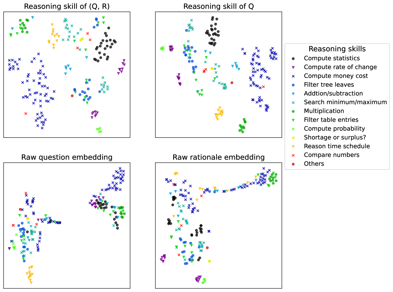<details> <summary>x1.png Details</summary>  ### Visual Description ## Scatter Plot Grid: Reasoning Skills and Embeddings ### Overview The image contains a 2x2 grid of scatter plots comparing reasoning skills and embeddings. Each plot uses distinct colored markers (circles, triangles, crosses) to represent different reasoning skills, with a shared legend on the right. The plots explore relationships between reasoning skills in different contexts: (Q, R), Q alone, raw question embeddings, and raw rationale embeddings. ### Components/Axes - **Legend**: Located on the right side, mapping 13 reasoning skills to colors and symbols: - **Black circles**: Compute statistics - **Purple triangles**: Compute rate of change - **Blue crosses**: Compute money cost - **Teal triangles**: Filter tree leaves - **Dark blue circles**: Addition/subtraction - **Green triangles**: Search minimum/maximum - **Yellow circles**: Multiplication - **Light green crosses**: Filter table entries - **Red circles**: Compute probability - **Orange triangles**: Shortage or surplus? - **Pink triangles**: Reason time schedule - **Red crosses**: Compare numbers - **Black dots**: Others - **Subplots**: 1. **Top-left**: "Reasoning skill of (Q, R)" – Dense clusters of multiple skills. 2. **Top-right**: "Reasoning skill of Q" – Dominated by black circles (compute statistics) and purple triangles (compute rate of change). 3. **Bottom-left**: "Raw question embedding" – Overlapping distributions with teal triangles (filter tree leaves) and blue crosses (compute money cost) forming distinct clusters. 4. **Bottom-right**: "Raw rationale embedding" – Linear trend with black circles (compute statistics) and orange triangles (shortage or surplus?) concentrated in the lower-left. ### Detailed Analysis - **Top-left Plot**: - **Distribution**: Scattered points across the plot, with teal triangles (filter tree leaves) and green triangles (search minimum/maximum) forming tight clusters in the upper-right quadrant. - **Trends**: No clear linear relationship; skills are broadly dispersed. - **Top-right Plot**: - **Distribution**: Black circles (compute statistics) dominate the center, while purple triangles (compute rate of change) cluster in the upper-right. Blue crosses (compute money cost) are sparse. - **Trends**: Compute statistics is the most frequent skill, followed by compute rate of change. - **Bottom-left Plot**: - **Distribution**: Teal triangles (filter tree leaves) and blue crosses (compute money cost) form distinct clusters in the lower-left and upper-right, respectively. Overlap occurs in the central region. - **Trends**: Filter tree leaves and compute money cost are spatially separated, suggesting distinct embeddings. - **Bottom-right Plot**: - **Distribution**: Black circles (compute statistics) and orange triangles (shortage or surplus?) form a linear trend from lower-left to upper-right. Red crosses (compare numbers) cluster in the lower-right. - **Trends**: Compute statistics and shortage/surplus? show a positive correlation. ### Key Observations 1. **Dominant Skills**: Compute statistics (black circles) appears most frequently across all plots. 2. **Clustering**: Skills like filter tree leaves (teal triangles) and compute money cost (blue crosses) show spatial separation in raw embeddings. 3. **Linear Relationship**: Compute statistics and shortage/surplus? exhibit a positive correlation in raw rationale embeddings. 4. **Symbol Consistency**: Symbols (circles, triangles, crosses) align with legend labels but lack explicit explanation for their meaning (e.g., data type or group). ### Interpretation The plots suggest that reasoning skills are context-dependent: - **Q vs. (Q, R)**: Skills like compute rate of change (purple triangles) are more prominent when considering only Q, while (Q, R) introduces additional skills like filter tree leaves (teal triangles). - **Embedding Relationships**: Raw question and rationale embeddings reveal distinct clusters for certain skills (e.g., filter tree leaves vs. compute money cost), indicating separable features in the data. - **Linear Correlation**: The positive trend between compute statistics and shortage/surplus? in raw rationale embeddings implies these skills may share underlying features or are often co-occurring in reasoning tasks. **Uncertainties**: - Axis labels are missing, preventing quantification of trends. - Symbol meanings (circles vs. triangles vs. crosses) are not explained, limiting interpretation of groupings. - Exact numerical values cannot be extracted without axis scales. </details> Figure 5: t-SNE projections of reasoning skills predicted from $(Q,R)$ (top-left), reasoning skills predicted from $Q$ (top-right), raw question embedding (bottom-left), and raw rationale embedding (bottom-right). The 12 different colors correspond to 12 skill labels provided by human. In TabMWP dataset, 200 examples are labeled based on the skills being showcased out of 12 manually-crafted skills labels, including “compute statistics”, “compute rate of change”, “Reason time schedule”, “Compute probability”, et. al. We investigate how the unsupervisedly discovered reasoning skills by LaRS align with human’s understanding of skills. More specifically, a visualization of how human-labeled skills distribute based on the t-SNE projections of four different types of embedding is shown in Fig. 5. Both the reasoning skill encoder (reasoning skill of $(Q,R)$ ) and the reasoning policy (reasoning skill of $Q$ ) trained by LaRS demonstrate clear separation of the labeled 12 skills. At the mean time, the human-labeled skills are not well-separated by raw question embedding, and even raw rationale embeddings. This indicates that the discovered reasoning skills aligns well with human-labeled skills even without explicit labels being provided during the training. This sheds the light on why the demonstration selection based on similar reasoning skills can improve the CoT prompting. 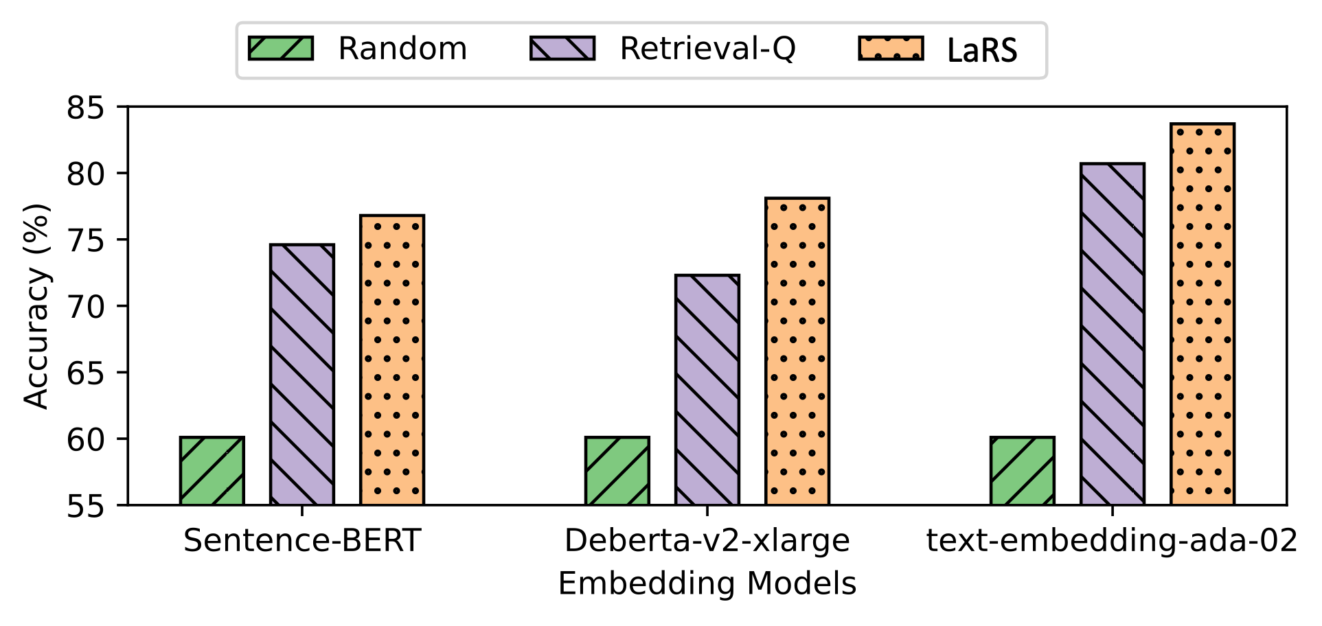<details> <summary>extracted/6556870/content/figures/ablation_embedding_model.png Details</summary>  ### Visual Description ## Bar Chart: Accuracy Comparison of Embedding Models by Method ### Overview The chart compares the accuracy (%) of three text embedding models (Sentence-BERT, Deberta-v2-xlarge, text-embedding-ada-02) using three methods: Random, Retrieval-Q, and LaRS. Accuracy is measured on a y-axis (55-85%), with models on the x-axis. Each model has three grouped bars representing the methods. ### Components/Axes - **X-axis**: Embedding Models (Sentence-BERT, Deberta-v2-xlarge, text-embedding-ada-02) - **Y-axis**: Accuracy (%) (55-85%, increments of 5%) - **Legend**: - Green (diagonal stripes): Random - Purple (diagonal stripes): Retrieval-Q - Orange (dots): LaRS - **Bar Patterns**: - Random: Green with diagonal stripes - Retrieval-Q: Purple with diagonal stripes - LaRS: Orange with dots ### Detailed Analysis 1. **Sentence-BERT**: - Random: ~60% - Retrieval-Q: ~75% - LaRS: ~77% 2. **Deberta-v2-xlarge**: - Random: ~60% - Retrieval-Q: ~72% - LaRS: ~78% 3. **text-embedding-ada-02**: - Random: ~60% - Retrieval-Q: ~81% - LaRS: ~84% ### Key Observations - **LaRS consistently outperforms** both Random and Retrieval-Q across all models. - **text-embedding-ada-02** achieves the highest accuracy (84%) with LaRS, followed by Deberta-v2-xlarge (78%) and Sentence-BERT (77%). - **Random method** shows minimal performance (~60%) for all models, serving as a baseline. - **Retrieval-Q** improves accuracy by ~15-20% over Random but remains ~5-7% below LaRS. ### Interpretation The data demonstrates that **LaRS significantly enhances accuracy** compared to other methods, with performance gains increasing as model complexity rises (text-embedding-ada-02 > Deberta-v2-xlarge > Sentence-BERT). This suggests LaRS is particularly effective for advanced embedding models. The consistent ~60% baseline for Random indicates minimal inherent accuracy without method-specific optimization. Retrieval-Q provides moderate improvements but does not match LaRS's efficacy, highlighting its potential as a mid-tier solution. The trend implies that method selection critically impacts performance, with LaRS being the optimal choice for high-accuracy applications. </details> (a) The accuracy of Random, Retrieval-Q, and, LaRS based on three different pre-trained embedding models. 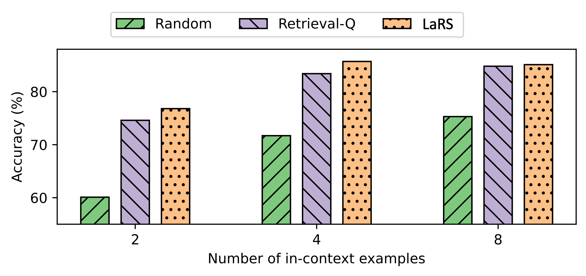<details> <summary>extracted/6556870/content/figures/ablation_num_example.png Details</summary>  ### Visual Description ## Bar Chart: Accuracy Comparison Across In-Context Examples ### Overview The chart compares the accuracy (%) of three methods—Random, Retrieval-Q, and LaRS—across three scenarios defined by the number of in-context examples (2, 4, 8). Accuracy is measured on the y-axis (55–90%), while the x-axis categorizes data by the number of examples. Each method is represented by a distinct color and pattern: green (Random), purple (Retrieval-Q), and orange (LaRS). ### Components/Axes - **X-axis**: "Number of in-context examples" with categories: 2, 4, 8. - **Y-axis**: "Accuracy (%)" ranging from 55% to 90%. - **Legend**: - Green (diagonal stripes): Random - Purple (diagonal stripes): Retrieval-Q - Orange (dots): LaRS - **Bar Groups**: Three clusters of bars, one for each x-axis category (2, 4, 8), with three bars per cluster (one per method). ### Detailed Analysis - **At 2 in-context examples**: - Random: ~60% accuracy (green bar). - Retrieval-Q: ~75% accuracy (purple bar). - LaRS: ~77% accuracy (orange bar). - **At 4 in-context examples**: - Random: ~72% accuracy (green bar). - Retrieval-Q: ~84% accuracy (purple bar). - LaRS: ~88% accuracy (orange bar). - **At 8 in-context examples**: - Random: ~75% accuracy (green bar). - Retrieval-Q: ~86% accuracy (purple bar). - LaRS: ~87% accuracy (orange bar). ### Key Observations 1. **Trends**: - All methods show increasing accuracy with more in-context examples. - LaRS and Retrieval-Q consistently outperform Random across all example counts. - LaRS and Retrieval-Q achieve near-identical accuracy at 8 examples (~87% vs. ~86%). 2. **Notable Patterns**: - Random’s accuracy plateaus at ~75% even with 8 examples, suggesting limited benefit from additional context. - LaRS and Retrieval-Q demonstrate diminishing returns between 4 and 8 examples (e.g., LaRS drops from ~88% to ~87%). ### Interpretation The data suggests that **LaRS and Retrieval-Q leverage in-context examples more effectively than Random**, likely due to structured retrieval or reasoning mechanisms. While all methods improve with more examples, the marginal gains for LaRS and Retrieval-Q at higher example counts imply potential saturation or diminishing utility of additional context. The slight edge of LaRS over Retrieval-Q at 4 examples (~88% vs. ~84%) may reflect architectural differences, but their convergence at 8 examples hints at similar performance ceilings. Random’s stagnation at ~75% underscores its inefficiency in utilizing context, possibly due to lack of targeted example selection. </details> (b) The accuracy of Random, Retrieval-Q, and LaRS using different number of in-context examples. Figure 6: Performances of three different selection methods under (a) different pre-trained embedding models, and (b) different number of in-context examples. #### Robustness to different pre-trained embedding models. Fig. 6(a) compares the performances of Random, Retrieval-Q, and LaRS based on three pre-trained embedding models, including Sentence-BERT Reimers and Gurevych (2019), Deberta-v2-xlarge, and, text-embedding-ada-02 Neelakantan et al. (2022) from OpenAI. We observe that the performances of retrieval-based selection methods monotonously improve with more capable pre-trained embedding models. However, our LaRS shows consistent improvements over Retrieval-Q given the same embedding models. #### Robustness to $k$ : the number of in-context examples. This study compares three selection methods, including Random, Retrieval-Q, and LaRS under three different number of in-context examples 2, 4, and 8. The results are summarized in Fig. 6(b). While the accuracy monotonously improves with the increasing number of in-context examples, LaRS consistently outperforms Retrieval-Q. #### How does Skill-KNN perform under stricter conditions? | Method Backbone: gpt-3.5-turbo Skill-KNN-large | TabMWP 78.3 +15.9 | GSM8K 75.0 –0.7 | Spider 58.4 +11.6 | COGS 94.6 +27.2 | | --- | --- | --- | --- | --- | | Skill-KNN-small | 75.5 +13.2 | 74.9 –0.8 | 37.3 –9.5 | 79.9 +12.7 | | Skill-KNN-zero | 77.7 +15.3 | 75.0 –0.7 | 49.0 +2.2 | 77.9 +10.8 | | LaRS (ours) | 78.1 +15.7 | 76.8 +1.1 | 53.0 +6.2 | 94.8 +27.2 | | Backbone: gpt-4o | | | | | | Skill-KNN-large | 80.6 +11.3 | 62.0 –0.2 | 56.3 +9.8 | 96.8 +23.4 | | Skill-KNN-small | 77.4 +8.1 | 62.3 +0.1 | 47.4 +0.3 | 79.4 +6.0 | | Skill-KNN-zero | 87.7 +0.1 | 78.6 –0.5 | 76.6 +2.5 | 78.1 +5.1 | | LaRS (ours) | 87.9 +0.3 | 78.3 +0.2 | 77.2 +3.1 | 90.2 +17.2 | | Backbone: claude-3-sonnet | | | | | | Skill-KNN-large | | 93.2 –0.1 | 25.9 +7.6 | 96.2 +17.0 | | Skill-KNN-small | | 92.3 –1.0 | 18.2 –0.1 | 86.6 +7.4 | | Skill-KNN-zero | 93.1 +0.5 | 92.1 –1.2 | 61.9 +0.2 | 86.6 +7.4 | | LaRS (ours) | 93.7 +1.1 | 93.6 +0.3 | 62.2 +0.5 | 96.9 +17.7 | | Backbone: claude-3-haiku | | | | | | Skill-KNN-zero | 93.3 +4.7 | 88.8 +0.2 | 61.0 +0.8 | 79.7 +13.5 | | LaRS (ours) | 93.3 +4.7 | 87.6 –1.0 | 61.3 +1.1 | 89.9 +23.7 | | Backbone: Falcon-40B-Instruct | | | | | | Skill-KNN-large | 55.9 +10.2 | 40.3 +1.5 | 23.7 +2.9 | 81.0 +35.9 | | Skill-KNN-small | 51.4 +5.7 | 36.5 –2.3 | 20.3 –0.3 | 59.4 +14.3 | | Skill-KNN-zero | 55.2 +9.5 | 38.7 –0.1 | 23.3 +2.7 | 82.1 +37.0 | | LaRS (ours) | 57.7 +12.0 | 39.1 +0.3 | 24.8 +4.2 | 89.5 +44.4 | Table 7: Skill-KNN-large, Skill-KNN-small, and Skill-KNN-zero compare with LaRS . ## Appendix D Case Study To explore the examples categorized as distinct skills within the learned latent reasoning skill representation, we employed K-means clustering on the latent reasoning skills of 1,000 examples from the TabMWP dataset. The centroids of these clusters are detailed in Table 8. The analysis presented in this table reveals that our method effectively discerns examples showcasing specific skills, such as “Searching minimum/maximum” and “Computing rate change”. | 0 | [TITLE]: School play committees Committee | Boys | Girls Casting | 17 | 5 Set design | 14 | 17 Lighting | 20 | 20 Costume | 7 | 4 Music | 2 | 13 | Some students at Dayton Middle School signed up to help out with the school play. Which committee has the most boys? Options: (A) set design (B) lighting (C) casting (D) costume | Search minimum/maximum | | --- | --- | --- | --- | | 1 | [TITLE]: Pairs of shoes per store Stem | Leaf 1 | 9 2 | 3, 3 3 | 0, 2 4 | 2, 4 5 | 5, 7 6 | 2, 5 7 | 7 8 | 0, 2, 4, 4 9 | 0, 0 | Ivan counted the number of pairs of shoes for sale at each of the shoe stores in the mall. How many stores have exactly 23 pairs of shoes? | Search tree leaves | | 2 | [TITLE]: None piece of licorice | $0.07 gum drop | $0.05 gumball | $0.08 cinnamon candy | $0.01 peppermint candy | $0.08 lemon drop | $0.07 | Derek has $0.06. Does he have enough to buy a piece of licorice and a cinnamon candy? Options: (A) yes (B) no | Compute money cost | | 3 | [TITLE]: None Number of offices | Number of chairs 1 | 2 2 | 4 3 | 6 4 | 8 5 | ? | Each office has 2 chairs. How many chairs are in 5 offices? | Multiplication | | 4 | [TITLE]: None popcorn balls | $1/kilogram coffee cake | $3/kilogram blueberry bars | $2/kilogram cream cheese bars | $2/kilogram lemon bars | $3/kilogram | Sarah went to the store and bought 2 kilograms of blueberry bars. How much did she spend? (Unit: $) | Compute money cost | | 5 | [TITLE]: None x | y 12 | 19 13 | 9 14 | 2 | The table shows a function. Is the function linear or nonlinear? Options: (A) linear (B) nonlinear | Compute rate of change | | 6 | [TITLE]: Tractors Farmer | Number of tractors Farmer Judy | 4 Farmer Joe | 7 Farmer Megan | 7 Farmer Rick | 4 Farmer Jane | 4 | Some farmers compared how many tractors they own. What is the mode of the numbers? | Compute statistics | | 7 | [TITLE]: None pink sweater | $6.69 pair of brown pants | $9.66 plaid scarf | $2.45 pair of sandals | $7.69 white polo shirt | $4.86 | How much money does Heather need to buy a pair of brown pants and a plaid scarf? (Unit: $) | Compute money cost | | 8 | [TITLE]: Tour bus schedule Location | Arrive | Depart the riverfront | 9:55 A.M. | 10:20 A.M. the zoo | 10:35 A.M. | 11:30 A.M. art museum | 12:05 P.M. | 12:30 P.M. science museum | 1:00 P.M. | 1:45 P.M. skyscraper | 1:50 P.M. | 2:20 P.M. governor’s mansion | 2:50 P.M. | 3:45 P.M. old building | 4:00 P.M. | 4:45 P.M. famous bridge | 5:15 P.M. | 5:40 P.M. the aquarium | 6:20 P.M. | 7:00 P.M. landmark sculpture | 7:45 P.M. | 8:20 P.M. | Look at the following schedule. Which stop does the bus depart from at 11.30 A.M.? Options: (A) zoo (B) riverfront (C) old building (D) science museum | Reason time schedule | | 9 | [TITLE]: None poppyseed muffin | $2.31 bowl of yogurt | $1.35 blueberry pancakes | $7.28 hash browns | $4.56 bowl of granola | $2.97 bagel with cream cheese | $2.56 | Max has $13.33. How much money will Max have left if he buys a bagel with cream cheese and blueberry pancakes? (Unit: $) | Compute money cost | | --- | --- | --- | --- | | 10 | [TITLE]: Balloons sold Day | Number of balloons Wednesday | 568 Thursday | 586 Friday | 558 Saturday | 565 | The manager of a party supply store researched how many balloons it sold in the past 4 days. On which day did the store sell the most balloons? Options: (A) Wednesday (B) Thursday (C) Friday (D) Saturday | Search minimum/maximum | | 11 | [TITLE]: None forklift | $9,987.00 dump truck | $9,543.00 race car | $8,370.00 crane | $6,996.00 bulldozer | $7,547.00 hydrofoil | $8,047.00 | How much more does a forklift cost than a dump truck? (Unit: $) | Compute money cost | Table 8: The closest examples to the 12 cluster centers computed by K-Means clustering method on reasoning skill latent variables. ## Appendix E Theoretical Analysis To prove Theorem 1, we start with the equation of rationale generation via CoT prompting, employing the skill-based demonstration selection method denoted as $g_{skill}$ . The process can be formalized as follows: $$ \displaystyle P_{M}( \displaystyle R\mid Q,g_{skill})=\int_{\mathcal{X}^{k}}P_{M}(R\mid pt)\Pi_{i=1 }^{k}[g_{skill}(Q_{i},R_{i}\mid Q)d(Q_{i},R_{i})] \tag{5} $$ where Equation 5 is integrated by substituting $pt=(Q_{1},R_{1},\cdots,Q_{k},R_{k},Q)$ as outlined in Equation 3, leading to: $$ \displaystyle P_{M}( \displaystyle R\mid Q,g_{skill})=\int_{\mathcal{Z}}P_{M}(R\mid z,Q)P_{M}(z\mid Q )\Pi_{i=1}^{k}[P_{skill}(z\mid Q)]dz \tag{6} $$ In this context, $P_{skill}(z\mid Q)$ is defined as: $$ \displaystyle P_{skill}(z\mid Q)=\int_{(Q^{\prime},R^{\prime})\in\mathcal{X}}P _{M}(z\mid Q^{\prime},R^{\prime})g_{skill}(Q^{\prime},R^{\prime}\mid Q)d(Q^{ \prime},R^{\prime})dz^{\prime} \tag{7} $$ Substituting the Definition 1 into Equation 7, leading to: $$ \displaystyle P_{skill}(z\mid Q)=\int_{(Q^{\prime},R^{\prime})\in\mathcal{X}} \int_{z^{\prime}\in\mathcal{Z}}P_{M}(z\mid Q^{\prime},R^{\prime})P_{E}(Q^{ \prime},R^{\prime}\mid z^{\prime})P_{E}(z^{\prime}\mid Q)dz^{\prime} \tag{8} $$ Applying Assumption 2 into the above equation, replacing $P_{M}(z\mid Q^{\prime},R^{\prime})$ with $P_{E}(z\mid Q^{\prime},R^{\prime})$ : $$ \displaystyle P_{skill}(z\mid Q) \displaystyle=\int_{(Q^{\prime},R^{\prime})\in\mathcal{X}}\int_{z^{\prime}\in \mathcal{Z}}P_{E}(z\mid Q^{\prime},R^{\prime})P_{E}(Q^{\prime},R^{\prime}\mid z ^{\prime})P_{E}(z^{\prime}\mid Q)dz^{\prime} \displaystyle=\int_{z^{\prime}\in\mathcal{Z}}\delta(z=z^{\prime})P_{E}(z^{ \prime}\mid Q)dz^{\prime} \displaystyle=P_{E}(z\mid Q) \tag{9} $$ By reintegrating the derived expression for $P_{skill}(z\mid Q)$ back into Equation 6, we arrive at: $$ \displaystyle P_{M}(R\mid Q,g_{skill})=\int_{\mathcal{Z}}P_{M}(R\mid z,Q)P_{M} (z\mid Q)\Pi_{i=1}^{k}[P_{E}(z\mid Q)]dz \tag{10} $$ Take the limit of $k\rightarrow\infty$ , above equation siplifies to: $$ \displaystyle P_{M}(R\mid Q,g_{skill})=\int_{\mathcal{Z}}P_{M}(R\mid z,Q)P_{E} (z\mid Q)dz \tag{11} $$ Applying Assumption 2 into the above equation, replacing $P_{M}(R\mid z,Q)$ with $P_{E}(R\mid z,Q)$ : $$ \displaystyle P_{M}(R\mid Q,g_{skill})=\int_{\mathcal{Z}}P_{E}(R\mid z,Q)P_{E} (z\mid Q)dz=P_{E}(R\mid Q) \tag{12} $$ According to Assumption 1, the example bank can approximate expert rationale generation, or $P_{E}(R\mid Q)=P^{*}(R\mid Q)$ , we then conclude: $$ \displaystyle P_{M}(R\mid Q,g_{skill})=P^{*}(R\mid Q) \tag{13} $$ Equation 13 means that the CoT prompting under the skill-based demonstration selection method give the optimal conditional distribution of rationales given questions by Definition 2. This proves the Theorem 1 under Assumption 1 and Assumption 2.