# SGLang: Efficient Execution of Structured Language Model Programs
**Authors**:
- Clark Barrett Ying Sheng (Stanford University UC Berkeley Shanghai Jiao Tong University)
> Equal contribution.
Abstract
Large language models (LLMs) are increasingly used for complex tasks that require multiple generation calls, advanced prompting techniques, control flow, and structured inputs/outputs. However, efficient systems are lacking for programming and executing these applications. We introduce SGLang, a system for efficient execution of complex language model programs. SGLang consists of a frontend language and a runtime. The frontend simplifies programming with primitives for generation and parallelism control. The runtime accelerates execution with novel optimizations like RadixAttention for KV cache reuse and compressed finite state machines for faster structured output decoding. Experiments show that SGLang achieves up to $6.4×$ higher throughput compared to state-of-the-art inference systems on various large language and multi-modal models on tasks including agent control, logical reasoning, few-shot learning benchmarks, JSON decoding, retrieval-augmented generation pipelines, and multi-turn chat. The code is publicly available at https://github.com/sgl-project/sglang.
1 Introduction
Recent increases in the capabilities of LLMs have broadened their utility, enabling them to tackle a wider range of general tasks and act as autonomous agents openai2023gpt4 ; bubeck2023sparks ; Park2023GenerativeAgents ; wang2023voyager ; sumers2023cognitive . In such applications, LLMs engage in multi-round planning, reasoning, and interaction with external environments. This is accomplished through tool usage schick2023toolformer ; patil2023gorilla , multiple input modalities team2023gemini ; alayrac2022flamingo , and a wide range of prompting techniques liu2023prompting , like few-shot learning brown2020language , self-consistency wang2022self , skeleton-of-thought ning2024skeletonofthought , and tree-of-thought yao2023tree . All of these new use cases require multiple, often dependent, LLM generation calls, showing a trend of using multi-call structures to complete complex tasks yao2022react ; kim2023llm .
The emergence of these patterns signifies a shift in our interaction with LLMs, moving from simple chatting to a more sophisticated form of programmatic usage of LLMs, which means using a program to schedule and control the generation processes of LLMs. We refer to these programs as "Language Model Programs" (LM Programs) beurer2023lmql ; khattab2023dspy . The advanced prompting techniques and agentic workflow mentioned above fall within the scope of LM programs. There are two common properties of LM programs: (1) LM programs typically contain multiple LLM calls interspersed with control flow. This is needed to complete complex tasks and improve overall quality. (2) LM programs receive structured inputs and produce structured outputs. This is needed to enable the composition of LM programs and to integrate LM programs into existing software systems.
Despite the widespread use of LM programs, current systems for expressing and executing them remain inefficient. We identify two primary challenges associated with the efficient use of LM programs: First, programming LM programs is tedious and difficult due to the non-deterministic nature of LLMs. Developing an LM program often requires extensive string manipulation, experimental tuning of prompts, brittle output parsing, handling multiple input modalities, and implementing parallelism mechanisms. This complexity significantly reduces the readability of even simple programs (Sec. 2).
Secondly and importantly, executing LM programs is inefficient due to redundant computation and memory usage. State-of-the-art inference engines (e.g., vLLM kwon2023vllm , TGI tgi , and TensorRT-LLM nvidia_tensorrt_llm ), have been optimized to reduce latency and improve throughput without direct knowledge of the workload. This makes these systems general and robust but also results in significant inefficiencies for any given workload. A prominent example is the reuse of the Key-Value (KV) cache (Sec. 3). The KV cache consists of reusable intermediate tensors that are essential for generative inference. During typical batch executions of LM programs, numerous opportunities exist to reuse the KV cache across multiple different LLM calls that share a common prefix. However, current systems lack effective mechanisms to facilitate this reuse, resulting in unnecessary computations and wasted memory. Another example is constrained decoding for structured outputs (e.g., JSON mode), where the output of LLMs is restricted to follow specific grammatical rules defined by a regular expression (Sec. 4). Under these constraints, multiple tokens can often be decoded once. However, existing systems only decode one token at a time, leading to suboptimal decoding speeds.
<details>
<summary>x1.png Details</summary>

### Visual Description
### Technical Diagram Analysis: SGLang Architecture
This image is a high-level architectural flow diagram illustrating the relationship between the frontend and backend components of the SGLang system. The flow moves linearly from left to right.
---
#### 1. Component Breakdown
The diagram consists of three primary blocks connected by directional arrows:
**A. SGLang Client (Frontend)**
* **Visual Properties:** Grey rectangular block with a thick black border.
* **Header Text:** **SGLang Client (Frontend)**
* **Content Text:** Language primitives (Sec. 2)
* *Note: "(Sec. 2)" is highlighted in blue text.*
**B. Interpreter**
* **Visual Properties:** Smaller yellow rectangular block with a black border, positioned in the center.
* **Content Text:** Interpreter
**C. SGLang Runtime (Backend)**
* **Visual Properties:** Large light-blue rectangular block with a black border.
* **Header Text:** **SGLang Runtime (Backend)**
* **Content Text:** Optimizations: RadixAttention (Sec. 3), Compressed finite state machines (Sec. 4), API speculative execution (Sec. 5)
* *Note: All section references ("Sec. 3", "Sec. 4", and "Sec. 5") are highlighted in blue text.*
---
#### 2. Flow and Logic
The diagram depicts a sequential pipeline:
1. **Input/Source:** The process begins at the **SGLang Client (Frontend)**, which handles "Language primitives".
2. **Transformation:** A black arrow points from the Client to the **Interpreter**. This indicates that the frontend primitives are passed to the Interpreter for processing.
3. **Execution/Output:** A second black arrow points from the Interpreter to the **SGLang Runtime (Backend)**. This indicates that the interpreted instructions are sent to the backend for execution.
4. **Backend Features:** The backend is responsible for three specific optimization techniques:
* **RadixAttention**
* **Compressed finite state machines**
* **API speculative execution**
---
#### 3. Text Transcription (Precise)
| Block Position | Header (Bold) | Body Text |
| :--- | :--- | :--- |
| **Left** | SGLang Client (Frontend) | Language primitives (Sec. 2) |
| **Center** | N/A | Interpreter |
| **Right** | SGLang Runtime (Backend) | Optimizations: RadixAttention (Sec. 3), Compressed finite state machines (Sec. 4), API speculative execution (Sec. 5) |
</details>
Figure 1: System architecture: An interpreter executes language primitives with optimized runtime.
To address these challenges, we present SGLang, a S tructured G eneration Lang uage for LLMs. The core idea is to systematically exploit the multi-call structure in LM programs for efficient execution. As shown in Fig. 1, it has two parts: a front-end language and a back-end runtime. The front-end simplifies the programming of LM programs, and the runtime accelerates their execution. The two parts can work together for better performance but can also function independently.
We introduce SGLang as a domain-specific language embedded in Python. It provides primitives for generation (e.g., extend, gen, select) and parallelism control (e.g., fork, join). SGLang is compatible with Python’s control flow and libraries, so users can develop advanced prompting workflows easily with native Python syntax. We provide an interpreter and a compiler for SGLang. The interpreter manages the prompt state as a stream and submits primitive operations to the stream for asynchronous execution, ensuring proper control over synchronization and intra-program parallelism. Additionally, SGLang program can be traced and compiled for more optimizations.
On the runtime side, we propose several novel optimizations to accelerate the execution of SGLang programs. The first technique, RadixAttention, enables the automatic reuse of the KV cache across multiple generation calls. In existing inference engines, the KV cache of a request is discarded after processing is completed, preventing the KV cache from being reused across multiple calls and significantly slowing down the execution. Instead, our system maintains an LRU cache of the KV cache for all requests within a radix tree. This approach manages the KV cache as a traditional cache and uses a radix tree for efficient matching, insertion, and eviction. It allows the runtime to handle various reuse patterns with a cache-aware scheduling policy efficiently. The second technique is a compressed finite state machine, which enables faster constrained decoding for structured outputs. Existing systems follow the constraints only for the next token by masking probabilities of disallowed tokens, making them able to decode only one token at a time. Instead, our system analyzes the constraints and builds a compressed finite-state machine to represent the constraint. This approach compresses a multi-token path into a single-step path whenever possible, allowing the decoding of multiple tokens at once to achieve faster decoding speed. Lastly, SGLang also supports API-only models like OpenAI’s GPT-4, and we introduce the third technique, API speculative execution, to optimize multi-call programs for API-only models.
Using SGLang, we implemented various LLM applications, including agent control, logical reasoning, few-shot learning benchmarks, JSON decoding, retrieval-augmented generation pipelines, multi-turn chat, and multi-modality processing. We tested the performance on models including Llama-7B/70B touvron2023llama2 , Mistral-8x7B jiang2024mixtral , LLaVA-v1.5-7B (image) liu2024llavanext , and LLaVA-NeXT-34B (video) zhang2024llavanextvideo on NVIDIA A10G and A100 GPUs. Experimental results show that SGLang achieves up to $6.4×$ higher throughput across a wide range of workloads, models, and hardware setups, compared to existing programming and inference systems, including Guidance guidance , vLLM kwon2023vllm , and LMQL beurer2023lmql .
2 Programming Model
This section introduces the SGLang programming model with a running example, describes its language primitives and execution modes, and outlines runtime optimization opportunities. This programming model can simplify tedious operations in multi-call workflows (e.g., string manipulation, API calling, constraint specification, parallelism) by providing flexible and composable primitives.
<details>
<summary>x2.png Details</summary>
### Visual Description
# Technical Document Extraction: SGLang Program Example
This image contains a code snippet written in a domain-specific language (likely SGLang) for orchestrating Large Language Model (LLM) workflows, accompanied by explanatory annotations.
## 1. Code Transcription
```python
dimensions = ["Clarity", "Originality", "Evidence"]
@function
def multi_dimensional_judge(s, path, essay):
s += system("Evaluate an essay about an image.")
s += user(image(path) + "Essay: " + essay)
s += assistant("Sure!")
# Return directly if it is not related
s += user("Is the essay related to the image?")
s += assistant(select("related", choices=["yes", "no"]))
if s["related"] == "no": return
# Judge multiple dimensions in parallel
forks = s.fork(len(dimensions))
for f, dim in zip(forks, dimensions):
f += user("Evaluate based on the following dimension: " +
dim + ". End your judgment with the word 'END'")
f += assistant("Judgment: " + gen("judgment", stop="END"))
# Merge the judgments
judgment = "\n".join(f["judgment"] for f in forks)
# Generate a summary and a grade. Return in the JSON format.
s += user("Provide the judgment, summary, and a letter grade")
s += assistant(judgment + "In summary," + gen("summary", stop=".")
+ "The grade of it is" + gen("grade"))
schema = r'\{"summary": "[\w\d\s]+\.", "grade": "[ABCD][+-]?"\}'
s += user("Return in the JSON format.")
s += assistant(gen("output", regex=schema))
state = multi_dimensional_judge.run(...)
print(state["output"])
```
## 2. Component Analysis and Annotations
The image uses yellow arrows to point from specific code blocks to descriptive text on the right side.
| Code Segment / Location | Annotation Text | Technical Significance |
| :--- | :--- | :--- |
| Initial `system`, `user`, and `assistant` calls | Handle chat template and multi-modal inputs | Demonstrates native support for images and structured chat roles. |
| `assistant(select("related", ...))` | Select an option with the highest probability | Shows constrained selection (classification) instead of free-form generation. |
| `if s["related"] == "no": return` | Fetch result; Use Python control flow | Highlights the integration of LLM outputs with standard Python logic. |
| `forks = s.fork(...)` | Runtime optimization: KV Cache Reuse (Sec. 3) | Indicates that forking allows multiple requests to share the prefix cache. |
| `gen("judgment", ...)` inside loop | Multiple generation calls run in parallel | Parallel execution of independent LLM generation tasks. |
| `"\n".join(f["judgment"] for f in forks)` | Fetch generation results | Aggregating data from parallel forks back into the main state. |
| `gen("summary")` and `gen("grade")` | Runtime optimization: API speculative execution (Sec. 5) | Suggests an optimization where multiple generations are predicted or batched. |
| `gen("output", regex=schema)` | Runtime optimization: fast constrained decoding (Sec. 4) | Use of Regular Expressions to force the LLM to output valid JSON. |
| `multi_dimensional_judge.run(...)` | Run an SGLang program | The entry point for executing the defined workflow. |
## 3. Workflow Summary
The program defines a multi-modal evaluation pipeline:
1. **Initialization:** Sets up a system prompt and inputs an image and an essay.
2. **Relevance Check:** Uses a `select` call to determine if the essay matches the image; exits early if not.
3. **Parallel Evaluation:** Forks the state to evaluate three dimensions ("Clarity", "Originality", "Evidence") simultaneously.
4. **Aggregation:** Joins the parallel judgments into a single string.
5. **Structured Output:** Generates a summary and a grade, then uses a regex schema to ensure the final output is a strictly formatted JSON object.
</details>
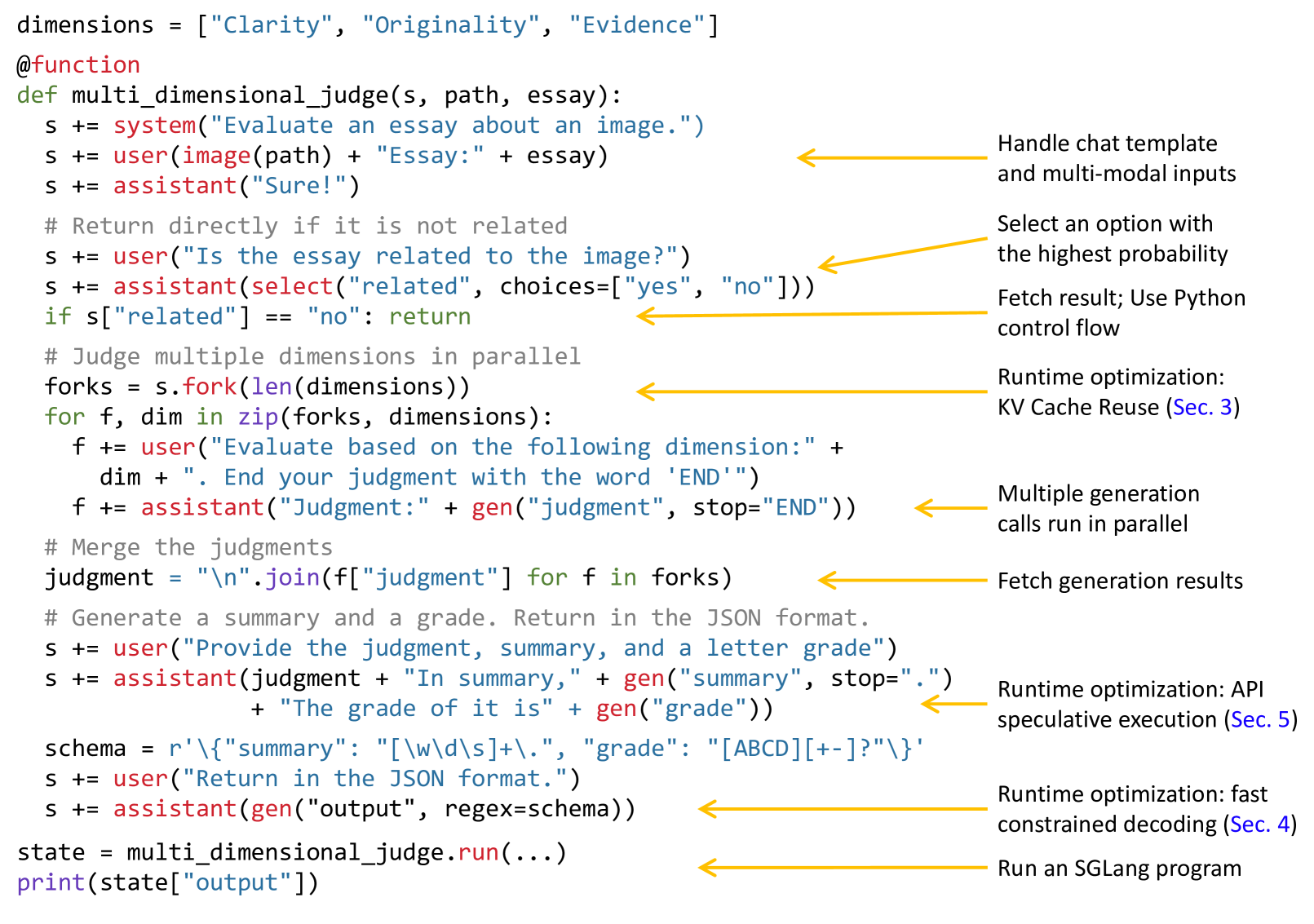
Figure 2: The implementation of a multi-dimensional essay judge in SGLang utilizes the branch-solve-merge prompting technique saha2023branch . Primitives provided by SGLang are shown in red.
A running example. The language is a domain-specific language embedded in Python. Fig. 2 shows a program that evaluates an essay about an image using the branch-solve-merge prompting method saha2023branch . The function multi_dimensional_judge takes three arguments: s, path, and essay. s manages the prompt state, path is the image file path, and essay is the essay text. New strings and SGLang primitives can be appended to the state s for execution using the += operator. First, the function adds the image and essay to the prompt. It then checks if the essay is related to the image using select, storing the result in s["related"]. If related, the prompt is forked into three copies for parallel evaluation from different dimensions, using gen to store results in f["judgment"]. Next, it merges the judgments, generates a summary, and assigns a letter grade. Finally, it returns the results in JSON format, following a schema defined by a regular expression constraint regex. SGLang greatly simplifies this program, as an equivalent program using an OpenAI API-like interface would take $2.1×$ as many lines of code due to manual string manipulation and parallelism control.
Language primitives. SGLang provides primitives for controlling prompt state, generation, and parallelism. They can be used together with Python syntax and libraries. Here are the primitives: “ gen ” calls a model to generate and stores the results in a variable with the name specified in its first argument. It supports a “ regex ” argument to constrain the output to follow a grammar defined by a regular expression (e.g., a JSON schema). “ select ” calls a model to choose the highest probability option from a list. The operator “ += ” or “ extend ” appends a string to the prompt. The operator “ [variable_name] ” fetches the results of a generation. “ fork ” creates parallel forks of the prompt state. “ join ” rejoins the prompt state. “ image ” and “ video ” take in image and video inputs.
Execution modes. The simplest way to execute an SGLang program is through an interpreter, where a prompt is treated as an asynchronous stream. Primitives like extend, gen, and select are submitted to the stream for asynchronous execution. These non-blocking calls allow Python code to continue running without waiting for the generation to finish. This is similar to launching CUDA kernels asynchronously. Each prompt is managed by a stream executor in a background thread, enabling intra-program parallelism. Fetching generation results will block until they are ready, ensuring correct synchronization. Alternatively, SGLang programs can be compiled as computational graphs and executed with a graph executor, allowing for more optimizations. This paper uses interpreter mode by default and discusses compiler mode results in Appendix D. SGLang supports open-weight models with its own SGLang Runtime (SRT), as well as API models such as OpenAI and Anthropic models.
Comparison. Programming systems for LLMs can be classified as high-level (e.g., LangChain, DSPy) and low-level (e.g., LMQL, Guidance, SGLang). High-level systems provide predefined or auto-generated prompts, such as DSPy’s prompt optimizer. Low-level systems typically do not alter prompts but allow direct manipulation of prompts and primitives. SGLang is a low-level system similar to LMQL and Guidance. Table 1 compares their features. SGLang focuses more on runtime efficiency and comes with its own co-designed runtime, allowing for novel optimizations introduced later. High-level languages (e.g., DSPy) can be compiled to low-level languages (e.g., SGLang). We demonstrate the integration of SGLang as a backend in DSPy for better runtime efficiency in Sec. 6.
Runtime optimizations. Fig. 2 shows three runtime optimization opportunities: KV cache reuse, fast constrained decoding, API speculative execution. We will discuss them in the following sections.
Table 1: Comparison among LMQL, Guidance, and SGLang.
| LMQL | Custom | extend, gen, select | HF Transformers, llama.cpp, OpenAI |
| --- | --- | --- | --- |
| Guidance | Python | extend, gen, select, image | HF Transformers, llama.cpp, OpenAI |
| SGLang | Python | extend, gen, select, image, video, fork, join | SGLang Runtime (SRT), OpenAI |
3 Efficient KV Cache Reuse with RadixAttention
SGLang programs can chain multiple generation calls and create parallel copies with the " fork " primitive. Additionally, different program instances often share some common parts (e.g., system prompts). These scenarios create many shared prompt prefixes during execution, leading to numerous opportunities for reusing the KV cache. During LLM inference, the KV cache stores intermediate tensors from the forward pass, reused for decoding future tokens. They are named after key-value pairs in the self-attention mechanism vaswani2017attention . KV cache computation depends only on prefix tokens. Therefore, requests with the same prompt prefix can reuse the KV cache, reducing redundant computation and memory usage. More background and some examples are provided in Appendix A.
Given the KV cache reuse opportunity, a key challenge in optimizing SGLang programs is reusing the KV cache across multiple calls and instances. While some systems explore certain KV cache reuse cases kwon2023vllm ; ye2024chunkattention ; juravsky2024hydragen ; gim2023prompt , they often need manual configurations and cannot handle all reuse patterns (e.g., dynamic tree structures). Consequently, most state-of-the-art inference systems recompute the KV cache for each request. We will discuss their limitations and our differences in Sec. 7.
This section introduces RadixAttention, a novel technique for automatic and systematic KV cache reuse during runtime. Unlike existing systems that discard the KV cache after a generation request finishes, our system retains the cache for prompts and generation results in a radix tree, enabling efficient prefix search, reuse, insertion, and eviction. We implement an LRU eviction policy and a cache-aware scheduling policy to enhance the cache hit rate. RadixAttention is compatible with techniques like continuous batching yu2022orca , paged attention kwon2023vllm , and tensor parallelism shoeybi2019megatron . In addition, it introduces only negligible memory and time overhead when there is no cache hit.
RadixAttention. A radix tree is a data structure that serves as a space-efficient alternative to a classical trie (prefix tree). Unlike typical trees, the edges of a radix tree can be labeled not just with single elements but also with sequences of elements of varying lengths, significantly enhancing efficiency. In our system, we utilize a radix tree to manage a mapping between sequences of tokens, and their corresponding KV cache tensors. These KV cache tensors are stored in a non-contiguous, paged layout, where the size of each page is equivalent to one token. Because GPU memory is quickly filled by the KV cahce, we introduce a simple LRU eviction policy that evicts the least recently used leaf first. By evicting leaves first, we enable the re-use of their common ancestors until those ancestors become leaves and are also evicted.
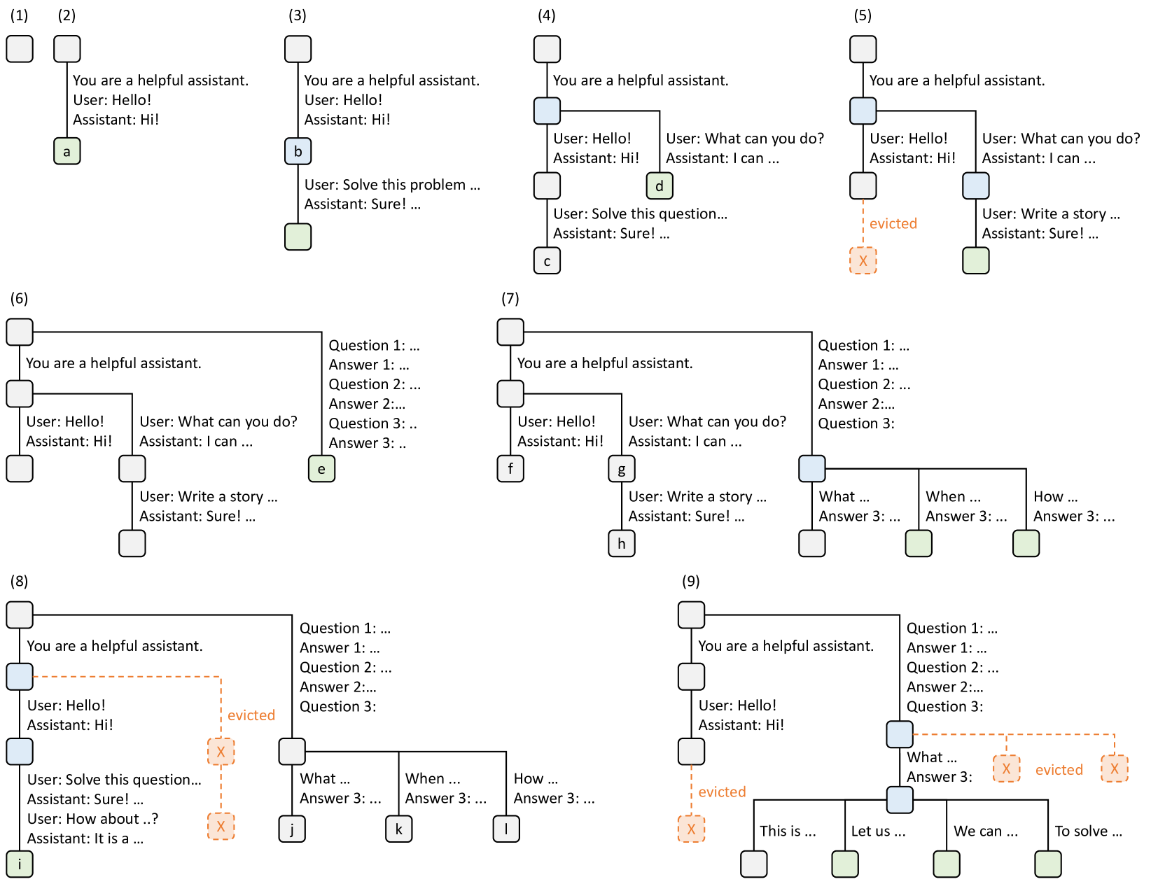
In the continuous batching setting, we cannot evict nodes used by the currently running batch. Therefore, each node maintains a reference counter indicating how many running requests are using it. A node is evictable if its reference counter is zero. Note that we do not preallocate a fixed-size memory pool as a cache. Instead, we let the cached tokens and the currently running requests share the same memory pool. Therefore, the system dynamically allocates memory for cache and running requests. When enough waiting requests run, the system will evict all cached tokens in favor of a larger batch size. Fig. 3 shows how the radix tree is maintained for several incoming requests. The frontend interpreter sends full prompts to the runtime, and the runtime performs prefix matching and reuse. The tree structure is stored on the CPU with negligible maintenance overhead. During the execution of the fork primitive, the frontend sends the prefix first as a hint, ensuring the prefix is correctly inserted into the tree. It then sends the remaining prompts. This "Frontend Hint" simplifies runtime scheduling and matching, exemplifying the benefits of frontend-runtime co-design.
<details>
<summary>x3.png Details</summary>
### Visual Description
# Technical Analysis: Hierarchical KV Cache Management and Eviction
This document describes a series of nine diagrams (labeled 1 through 9) illustrating the management of a hierarchical Key-Value (KV) cache in a Large Language Model (LLM) context. The diagrams show how system prompts, conversation histories, and branching queries are stored, shared, and evicted.
## Visual Legend and Component Key
* **Grey Rounded Square:** Represents a cached block of text/tokens.
* **Light Blue Rounded Square:** Represents a shared parent node in a branching conversation.
* **Light Green Rounded Square with Letter:** Represents the current active leaf node or "head" of a specific conversation thread.
* **Orange Dashed Square with 'X':** Represents a cache block that has been **evicted** from memory.
* **Solid Black Lines:** Represent the hierarchical relationship (parent-child) between blocks.
* **Orange Dashed Lines:** Represent the link to an evicted block.
---
## Sequence Analysis
### (1) Initial State
* A single empty or root cache block is initialized.
### (2) Linear Conversation Start
* **Root:** System prompt: "You are a helpful assistant."
* **Child Node [a]:** Contains "User: Hello! Assistant: Hi!"
* **Structure:** A simple linear chain.
### (3) Linear Extension
* **Root:** System prompt.
* **Intermediate Node [b]:** "User: Hello! Assistant: Hi!"
* **Leaf Node:** "User: Solve this problem ... Assistant: Sure! ..."
* **Trend:** The conversation grows linearly by appending a new block.
### (4) Branching Conversation
* The cache branches from the first interaction.
* **Shared Parent (Blue):** "User: Hello! Assistant: Hi!"
* **Branch 1 (Left):** Leads to node **[c]** with "User: Solve this question... Assistant: Sure! ..."
* **Branch 2 (Right):** Leads to node **[d]** with "User: What can you do? Assistant: I can ..."
### (5) Cache Eviction (Branch 1)
* **Shared Parent (Blue):** Remains in cache.
* **Branch 1 (Left):** The leaf node is replaced by an orange dashed box marked **"X"** and labeled **"evicted"**.
* **Branch 2 (Right):** Continues to grow. A new leaf node is added: "User: Write a story ... Assistant: Sure! ..."
### (6) Complex Branching (Three Threads)
* The root "You are a helpful assistant" now has two main branches.
* **Left Branch:** Further sub-branches into two conversations (one ending in a green leaf, one in a grey block).
* **Right Branch [e]:** A new thread containing "Question 1: ... Answer 1: ... Question 2: ... Answer 2: ... Question 3: ... Answer 3: ..."
### (7) Multi-Level Branching
* The right-most branch from step (6) now acts as a shared parent (Blue) for three new sub-queries:
* **Sub-branch 1:** "What ... Answer 3: ..."
* **Sub-branch 2:** "When ... Answer 3: ..." (Green leaf)
* **Sub-branch 3:** "How ... Answer 3: ..." (Green leaf)
* Nodes **[f]**, **[g]**, and **[h]** represent the leaf nodes of the left-side branches.
### (8) Deep Eviction and Linear Growth
* **Left Branch:** The middle section of the conversation is **evicted** (Orange 'X'). However, a new leaf node **[i]** is generated further down: "User: Solve this question... Assistant: Sure! ... User: How about ..? Assistant: It is a ...".
* **Right Branch:** The three sub-queries from step (7) are now leaf nodes **[j]**, **[k]**, and **[l]**.
### (9) Massive Eviction and Wide Branching
* **Left Branch:** The entire middle segment is **evicted**.
* **Right Branch:**
* The parent node for the "What/When/How" queries is **evicted**.
* Two subsequent sub-nodes are also **evicted**.
* A new shared parent (Blue) is created at the bottom right, branching into four distinct green leaf nodes: "This is ...", "Let us ...", "We can ...", and "To solve ...".
---
## Summary of Data Trends
1. **Prefix Sharing:** Identical starting strings (like the system prompt) are stored once and shared across all branches to save memory.
2. **Dynamic Branching:** The system supports multiple simultaneous conversation paths originating from any point in the history.
3. **Selective Eviction:** When memory is full, the system evicts specific blocks (marked 'X'). The diagrams suggest that leaf nodes or intermediate nodes can be evicted while keeping the root or other active branches intact.
4. **Recovery/Re-growth:** Even after eviction (as seen in step 8 and 9), the tree can continue to grow from remaining valid nodes.
</details>
Figure 3: Examples of RadixAttention operations with an LRU eviction policy, illustrated across nine time points. The figure demonstrates the dynamic evolution of the radix tree in response to various requests. These requests include two chat sessions, a batch of few-shot learning inquiries, and a self-consistency sampling. Each tree edge carries a label denoting a substring or a sequence of tokens. The nodes are color-coded to reflect different states: green for newly added nodes, blue for cached nodes accessed during the time point, and red for nodes that have been evicted. In step (1), the radix tree is initially empty. In step (2), the server processes an incoming user message "Hello" and responds with the LLM output "Hi". The system prompt "You are a helpful assistant", the user message "Hello!", and the LLM reply "Hi!" are consolidated into the tree as a single edge linked to a new node. In step (3), a new prompt arrives and the server finds the prefix of the prompt (i.e., the first turn of the conversation) in the radix tree and reuses its KV cache. The new turn is appended to the tree as a new node. In step (4), a new chat session begins. The node “b” from (3) is split into two nodes to allow the two chat sessions to share the system prompt. In step (5), the second chat session continues. However, due to the memory limit, node "c" from (4) must be evicted. The new turn is appended after node "d" in (4). In step (6), the server receives a few-shot learning query, processes it, and inserts it into the tree. The root node is split because the new query does not share any prefix with existing nodes. In step (7), the server receives a batch of additional few-shot learning queries. These queries share the same set of few-shot examples, so we split node ’e’ from (6) to enable sharing. In step (8), the server receives a new message from the first chat session. It evicts all nodes from the second chat session (node "g" and "h") as they are least recently used. In step (9), the server receives a request to sample more answers for the questions in node "j" from (8), likely for self-consistency prompting. To make space for these requests, we evict node "i", "k", and "l" in (8).
Cache-aware scheduling. We define the cache hit rate as $\frac{\text{number of cached prompt tokens}}{\text{number of prompt tokens}}$ . When there are many requests in the waiting queue, the order in which they are executed can significantly impact the cache hit rate. For example, if the request scheduler frequently switches between different, unrelated requests, it can lead to cache thrashing and a low hit rate. We design a cache-aware scheduling algorithm to increase the cache hit rate. In the batch-processing setting we sort the requests by matched prefix length and prioritize requests with longer matched prefixes instead of using a first-come, first-served schedule. Alg. 1 (Appendix) shows the pseudo-code for cache-aware scheduling with contiguous batching. The algorithm uses longest-shared-prefix-first order. In more latency-sensitive settings we may still be able to tolerate limited batch re-ordering to improve cache reuse. Additionally, we prove the following theorem for optimal scheduling in the offline case. In practice, the computation is not the same as what is described in the proof of Theorem 3.1 because the unpredictable number of output tokens can cause the recomputation of the KV cache.
**Theorem 3.1**
*For a batch of requests, we can achieve an optimal cache hit rate by visiting the radix tree of the requests in the depth-first search order, with a cache size $≥$ the maximum request length. The longest-shared-prefix-first order is equivalent to a depth-first search order.*
The proof is in Sec. A.3 (Appendix). In the online case, the DFS order will be disrupted, but our schedule still approximates the DFS behavior on the augmented part of the full radix tree, as described in Sec. A.3. While greedy cache-aware scheduling can achieve high throughput, it can lead to starvation. We leave its integration with other fair scheduling methods sheng2023fairness as future work.
Distributed Cases. RadixAttention can be extended to multiple GPUs. For tensor parallelism, each GPU maintains a sharded KV cache. There is no need for additional synchronization because the tree operations are the same. Data parallelism with multiple workers is discussed in Sec. A.4 (Appendix).
4 Efficient Constrained Decoding with Compressed Finite State Machine
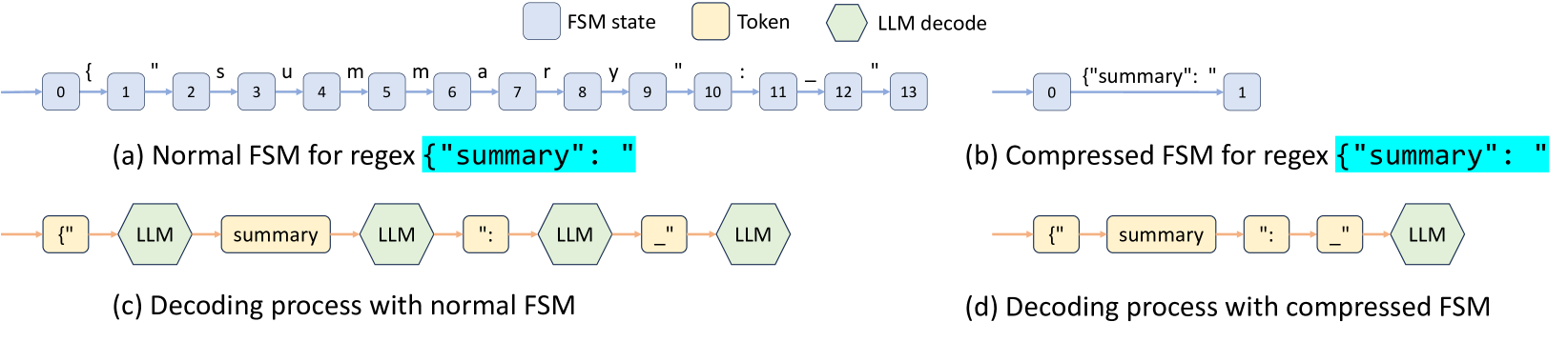
In LM programs, users often want to constrain the model’s output to follow specific formats, such as JSON schemas. This can improve controllability and robustness, and make the output easier to parse. SGLang offers a regex argument to enforce such constraints using regular expressions, which are expressive enough for many practical scenarios. Existing systems support this by converting a regular expression into a finite state machine (FSM) willard2023efficient . During decoding, they maintain the current FSM state, retrieve allowed tokens from the next states, and set the probability of invalid tokens to zero, decoding token by token. This token-by-token approach, however, is inefficient when there are opportunities to decode multiple tokens at once. For example, the constant sequence {"summary": " in Fig. 2 spans multiple tokens in the normal decoding process as shown in Fig. 4 (c), requiring multiple decoding stages, even though there is only one valid next token when decoding it. Therefore, the whole sequence can be decoded in a single step (i.e., forward pass). However, existing systems can only decode one token at a time because the lack of integration between the FSM and the model runner in existing systems prevents multi-token processing, resulting in slow decoding.
<details>
<summary>x4.png Details</summary>
### Visual Description
# Technical Document Extraction: FSM and LLM Decoding Comparison
This document describes a technical diagram illustrating the optimization of Finite State Machines (FSM) for Large Language Model (LLM) decoding processes, specifically for regex-constrained generation.
## 1. Legend and Component Definitions
The diagram uses color-coded and shape-coded blocks to represent different stages of the process:
* **FSM state (Light Blue Rectangle):** Represents a discrete state within a Finite State Machine.
* **Token (Light Yellow Rectangle):** Represents a specific string or character sequence processed as a unit.
* **LLM decode (Light Green Hexagon):** Represents the computational step where the Large Language Model generates/decodes a token.
---
## 2. Diagram Analysis by Section
### Section (a): Normal FSM for regex `{"summary": "`
This section shows a linear, character-by-character state transition for a specific JSON-like string.
* **Flow:** A sequence of 14 states (numbered 0 through 13) connected by blue arrows.
* **Transitions:** Each arrow represents a single character transition:
* 0 → 1: `{`
* 1 → 2: `"`
* 2 → 3: `s`
* 3 → 4: `u`
* 4 → 5: `m`
* 5 → 6: `m`
* 6 → 7: `a`
* 7 → 8: `r`
* 8 → 9: `y`
* 9 → 10: `"`
* 10 → 11: `:`
* 11 → 12: `_` (space character)
* 12 → 13: `"`
### Section (b): Compressed FSM for regex `{"summary": "`
This section demonstrates the optimization of the FSM by collapsing multiple character transitions into a single state jump.
* **Flow:** A direct transition from state **0** to state **1**.
* **Transition Label:** The entire string `{"summary": "` is handled in a single transition step.
### Section (c): Decoding process with normal FSM
This section illustrates the interaction between the LLM and the unoptimized FSM.
* **Sequence:**
1. **Token:** `{"`
2. **LLM decode**
3. **Token:** `summary`
4. **LLM decode**
5. **Token:** `":`
6. **LLM decode**
7. **Token:** `_"` (space and quote)
8. **LLM decode**
* **Trend:** The process is fragmented, requiring four separate LLM decoding steps to complete the sequence because the FSM operates at a fine-grained level.
### Section (d): Decoding process with compressed FSM
This section illustrates the interaction between the LLM and the optimized FSM.
* **Sequence:**
1. **Token:** `{"`
2. **Token:** `summary`
3. **Token:** `":`
4. **Token:** `_"` (space and quote)
5. **LLM decode**
* **Trend:** The tokens are processed sequentially without interruption. The LLM decoding step only occurs once at the end of the pre-defined sequence.
---
## 3. Summary of Key Information
* **Objective:** To compare "Normal" vs. "Compressed" FSMs in the context of LLM decoding.
* **Key Data Point:** The compressed FSM (b) reduces a 13-step character transition into a single transition.
* **Process Efficiency:** The decoding process with a compressed FSM (d) significantly reduces the number of LLM decoding calls compared to the normal process (c), which requires an LLM call after almost every token segment.
* **Textual Content:** The primary regex being processed is `{"summary": "`. Note that in the diagram, the space character is represented by an underscore `_` in the transition labels.
</details>
Figure 4: The decoding process of normal and compressed FSMs (the underscore _ means a space).
SGLang overcomes this limitation by creating a fast constrained decoding runtime with a compressed FSM. This runtime analyzes the FSM and compresses adjacent singular-transition edges in the FSM into single edges as demonstrated in Fig. 4 (b), allowing it to recognize when multiple tokens can be decoded together. In Fig. 4 (d), multiple tokens on the compressed transition edge can be decoded in one forward pass, which greatly accelerates the decoding process. It is also general and applicable to all regular expressions. More details on the background and implementation are in Appendix B.
5 Efficient Endpoint Calling with API Speculative Execution
The previous sections introduced optimizations for open-weight models, which require modifications to the model inference process. Additionally, SGLang works with API-access-only models, such as OpenAI’s GPT-4. However, for these models, we can only call a black-box API endpoint.
This section introduces a new optimization for black-box API models that accelerates execution and reduces the API cost of multi-call SGLang programs using speculative execution. For example, a program may ask the model to generate a description of a character with a multi-call pattern: s += context + "name:" + gen("name", stop="\n") + "job:" + gen("job", stop="\n"). Naively, the two gen primitives correspond to two API calls, meaning that the user needs to pay for the input token fee on the context twice. In SGLang, we can enable speculative execution on the first call and let it continue the generation of a few more tokens by ignoring the stop condition. The interpreter keeps the additional generation outputs and matches and reuses them with later primitives. In certain cases, with careful prompt engineering, the model can correctly match the template with high accuracy, saving us the latency and input costs of one API call.
6 Evaluation
We evaluate the performance of SGLang across diverse LLM workloads. Subsequently, we conduct ablation studies and case studies to demonstrate the effectiveness of specific components. SGLang is implemented in PyTorch paszke2019pytorch with custom CUDA kernels from FlashInfer flashinfer and Triton tillet2019triton .
6.1 Setup
Models. We test dense Llama-2 models touvron2023llama2 , sparse mixture of experts Mixtral models jiang2024mixtral , multi-modal LLaVA image liu2023improved and video models zhang2024llavanextvideo , and API model OpenAI’s GPT-3.5. For open-weight models, the number of parameters ranges from 7 billion to 70 billion, and we use float16 precision.
Hardware. We run most experiments on AWS EC2 G5 instances, which are equipped with NVIDIA A10G GPUs (24GB). We run 7B models on a single A10G GPU and larger models on multiple A10G GPUs with tensor parallelism shoeybi2019megatron . We run some additional experiments on A100G (80GB) GPUs.
Baselines. We compare SGLang against both high-level programming systems with their respective languages and default runtimes, as well as low-level inference engines with standard OpenAI-like Completion APIs. Unless otherwise stated, we do not turn on optimizations that will change the computation results so that all systems compute the same results. The baselines include:
- Guidance guidance , a language for controlling LLMs. We use Guidance v0.1.8 with llama.cpp backend.
- vLLM kwon2023vllm , a high-throughput inference engine. We use vLLM v0.2.5 and its default API server RadixAttention has been partially integrated as an optional experimental feature into the latest version of vLLM; therefore, we used an earlier version for comparison..
- LMQL beurer2023lmql , a query language. We use LMQL v0.7.3 with Hugging Face Transformers backend.
Workloads. We test the following: 5-shot MMLU hendrycks2020measuring and 20-shot HellaSwag zellers2019hellaswag benchmarks. We decode one token for MMLU and use primitive select to select the answer with the highest probability for HellaSwag. For the ReAct agent yao2022react and generative agents Park2023GenerativeAgents , we extract the traces from the original papers and replay them. We use the Tree-of-thought yao2023tree for the GSM-8K problems and Skeleton-of-thought ning2024skeletonofthought for tip generation. We use LLM judges with the branch-solve-merge saha2023branch technique; JSON decoding with a schema specified by a regular expression; Multi-turn chat with 4 turns, where the input of each turn is randomly sampled between 256-512 tokens. Multi-turn chat (short) means short output (4-8 tokens) and multi-turn chat (long) means long output (256-512 tokens); DSPy retrieval-augmented generation (RAG) pipeline khattab2023dspy in its official example.
Metrics. We report two performance metrics: throughput and latency. For throughput, we run a sufficiently large batch of program instances to compute the maximum throughput, comparing the number of program instances executed per second (programs per second, p/s). For latency, we execute a single program at a time without batching and report the average latency for multiple instances.
<details>
<summary>x5.png Details</summary>
### Visual Description
# Technical Data Extraction: Throughput Comparison Chart
## 1. Image Overview
This image is a grouped bar chart comparing the normalized throughput of four different Large Language Model (LLM) inference/programming frameworks across eleven distinct benchmarks or tasks.
## 2. Component Isolation
### Header (Legend)
* **Location:** Top center of the image.
* **SGLang:** Orange bar (Reference baseline at 1.0).
* **vLLM:** Green bar.
* **Guidance:** Blue bar.
* **LMQL:** Grey bar.
### Main Chart Area
* **Y-Axis Label:** Throughput (Normalized)
* **Y-Axis Scale:** 0.0 to 1.0 (increments of 0.2 marked: 0.0, 0.2, 0.5, 0.8, 1.0). Note: The "0.5" marker is placed where 0.4 would typically be, and "0.8" where 0.6 would be, suggesting a non-linear or custom visual spacing, though the bars represent relative ratios.
* **X-Axis Categories (Benchmarks):**
1. MMLU
2. ReAct Agents
3. Generative Agents
4. Tree of Thought
5. Skeleton of Thought
6. LLM Judge
7. HellaSwag
8. JSON Decoding
9. Multi-Turn Chat (short)
10. Multi-Turn Chat (long)
11. DSPy RAG Pipeline
## 3. Data Extraction and Trend Analysis
**Trend Verification:** In every category, **SGLang (Orange)** maintains the maximum normalized value of 1.0. All other frameworks (**vLLM**, **Guidance**, **LMQL**) show significantly lower throughput relative to the SGLang baseline across all tested benchmarks.
</details>
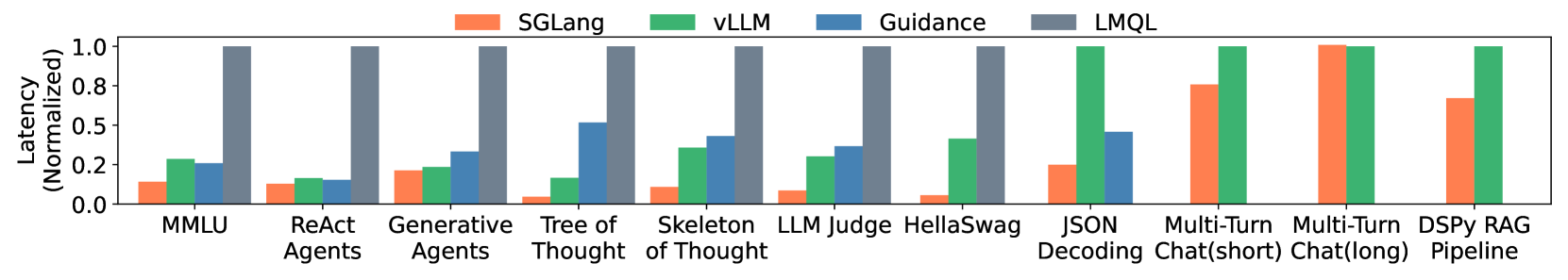
Figure 5: Normalized throughput on Llama-7B models. Higher is better.
<details>
<summary>x6.png Details</summary>
### Visual Description
# Technical Data Extraction: Normalized Latency Comparison
## 1. Image Overview
This image is a grouped bar chart comparing the normalized latency of four different Large Language Model (LLM) inference and programming frameworks across eleven distinct benchmarks/tasks.
## 2. Component Isolation
### Header (Legend)
The legend is positioned at the top center of the image.
* **SGLang** (Orange/Coral): `[x: ~30%, y: top]`
* **vLLM** (Green): `[x: ~45%, y: top]`
* **Guidance** (Blue): `[x: ~60%, y: top]`
* **LMQL** (Grey): `[x: ~75%, y: top]`
### Main Chart Area
* **Y-Axis Title:** Latency (Normalized)
* **Y-Axis Markers:** 0.0, 0.2, 0.5, 0.8, 1.0
* **X-Axis Categories (Benchmarks):**
1. MMLU
2. ReAct Agents
3. Generative Agents
4. Tree of Thought
5. Skeleton of Thought
6. LLM Judge
7. HellaSwag
8. JSON Decoding
9. Multi-Turn Chat(short)
10. Multi-Turn Chat(long)
11. DSPy RAG Pipeline
## 3. Data Extraction and Trend Analysis
The chart uses normalized values where the slowest framework for a given task typically represents the baseline of 1.0. Lower bars indicate better performance (lower latency).
### Trend Verification by Series
* **SGLang (Orange):** Consistently the lowest or near-lowest latency across all benchmarks. It shows significant performance leads in complex reasoning tasks like "Tree of Thought" and "HellaSwag."
* **vLLM (Green):** Generally higher latency than SGLang but lower than Guidance/LMQL in early benchmarks. It becomes the baseline (1.0) for the final three chat and RAG benchmarks.
* **Guidance (Blue):** Mid-range latency. It is absent from the final three benchmarks.
* **LMQL (Grey):** Consistently the highest latency (1.0) for the first seven benchmarks, after which it is absent from the data.
### Reconstructed Data Table (Approximate Values)
| Benchmark | SGLang (Orange) | vLLM (Green) | Guidance (Blue) | LMQL (Grey) |
| :--- | :---: | :---: | :---: | :---: |
| **MMLU** | ~0.15 | ~0.28 | ~0.25 | 1.0 |
| **ReAct Agents** | ~0.12 | ~0.18 | ~0.15 | 1.0 |
| **Generative Agents** | ~0.20 | ~0.22 | ~0.35 | 1.0 |
| **Tree of Thought** | ~0.05 | ~0.18 | ~0.52 | 1.0 |
| **Skeleton of Thought** | ~0.10 | ~0.35 | ~0.42 | 1.0 |
| **LLM Judge** | ~0.08 | ~0.30 | ~0.38 | 1.0 |
| **HellaSwag** | ~0.05 | ~0.42 | N/A | 1.0 |
| **JSON Decoding** | ~0.25 | 1.0 | ~0.45 | N/A |
| **Multi-Turn Chat(short)** | ~0.80 | 1.0 | N/A | N/A |
| **Multi-Turn Chat(long)** | 1.0 | ~0.98 | N/A | N/A |
| **DSPy RAG Pipeline** | ~0.70 | 1.0 | N/A | N/A |
## 4. Key Observations
* **Framework Availability:** LMQL and Guidance data points are missing for the more complex/recent benchmarks (JSON Decoding through DSPy RAG Pipeline).
* **SGLang Performance:** SGLang demonstrates a substantial latency reduction (often >5x faster) compared to the baseline (LMQL) in the first seven tasks.
* **Scaling:** In "Multi-Turn Chat(long)", SGLang and vLLM perform almost identically, with SGLang slightly higher, whereas in "DSPy RAG Pipeline", SGLang regains a lead over vLLM.
</details>
Figure 6: Normalized latency on Llama-7B models. Lower is better.
6.2 End-to-End Performance
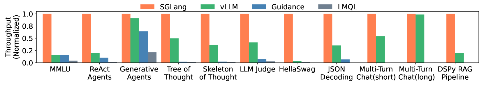
Results on open-weight models. The latency and throughput results are shown in Fig. 5 and Fig. 6. SGLang improves throughput by up to $6.4×$ and reduces latency by up to $3.7×$ . These improvements result from KV cache reuse, the exploitation of parallelism within a single program, and faster constrained decoding. Next, we explain the reasons for the speedup in each benchmark.
On MMLU, SGLang can reuse the KV cache of the 5-shot examples with RadixAttention. RadixAttention benefits both throughput and latency. RadixAttention reduces total memory usage by sharing the KV cache, allowing for a larger batch size to improve maximum throughput. RadixAttention also reduces the computation of prefill, thus decreasing the first token latency. On HellaSwag, SGLang reuses the KV cache of both few-shot examples and the common question prefix for multiple choices, resulting in two-level sharing. For the ReAct and generative agents, SGLang reuses the KV cache of the agent template and previous calls. On Tree-of-thought and Skeleton-of-thought, SGLang parallelizes the generation calls within a single program and reuses the KV cache as much as possible. On JSON decoding, SGLang accelerates decoding by decoding multiple tokens at once with a compressed finite state machine. In multi-turn chat, SGLang reuses the KV cache of the chat history. The speedup is more noticeable for short outputs because KV cache reuse mostly helps reduce the prefix time. For long outputs, because there is not much sharing between different chat sessions and the decoding time dominates, there is almost no speedup. In the DSPy RAG pipeline, SGLang reuses the KV cache of the common context example. On these benchmarks, the cache hit rate ranges from 50% to 99%. Fig. 13 (Appendix) lists the achieved and optimal cache hit rates for all of them, showing that our cache-aware scheduling approaches 96% of the optimal hit rate on average.
We exclude LMQL and Guidance from some of the last five benchmarks due to slow performance and missing functionalities. LMQL’s issues stem from slow token-level processing and an unoptimized backend, while Guidance lacks batching and parallelism support.
<details>
<summary>x7.png Details</summary>
### Visual Description
# Technical Data Extraction: Throughput Comparison Chart
## 1. Image Overview
This image is a grouped bar chart comparing the normalized throughput of two software frameworks, **SGLang** and **vLLM**, across eleven different Large Language Model (LLM) benchmarks and tasks.
## 2. Component Isolation
### Header / Legend
* **Location:** Top center of the chart.
* **Legend Items:**
* **SGLang:** Represented by an orange bar.
* **vLLM:** Represented by a green bar.
### Main Chart Area
* **Y-Axis Label:** Throughput (Normalized)
* **Y-Axis Scale:** Linear, ranging from 0.0 to 1.0 with markers at [0.0, 0.2, 0.5, 0.8, 1.0].
* **X-Axis Categories:** Eleven distinct benchmarks/tasks.
* **Data Representation:** For every category, SGLang is normalized to 1.0 (full height), and vLLM is shown as a relative fraction of that performance.
## 3. Data Table Extraction
The following table reconstructs the visual data points. Values for vLLM are estimated based on their alignment with the Y-axis markers.
| Benchmark / Task | SGLang (Orange) | vLLM (Green) | Visual Trend Description |
| :--- | :---: | :---: | :--- |
| **MMLU** | 1.0 | ~0.15 | SGLang significantly outperforms vLLM. |
| **ReAct Agents** | 1.0 | ~0.12 | SGLang significantly outperforms vLLM. |
| **Generative Agents** | 1.0 | ~0.68 | vLLM performs relatively well but remains lower than SGLang. |
| **Tree of Thought** | 1.0 | ~0.30 | SGLang maintains a large lead. |
| **Skeleton of Thought** | 1.0 | ~0.68 | vLLM performance is higher here than in most other tasks. |
| **LLM Judge** | 1.0 | ~0.35 | SGLang is approximately 3x faster. |
| **HellaSwag** | 1.0 | ~0.03 | vLLM shows near-zero throughput relative to SGLang. |
| **JSON Decoding** | 1.0 | ~0.10 | SGLang significantly outperforms vLLM. |
| **Multi-Turn Chat (short)** | 1.0 | ~0.45 | vLLM reaches nearly half the throughput of SGLang. |
| **Multi-Turn Chat (long)** | 1.0 | ~0.60 | vLLM performance improves relative to the short chat task. |
| **DSPy RAG Pipeline** | 1.0 | ~0.12 | SGLang significantly outperforms vLLM. |
## 4. Key Findings and Trends
* **Baseline Performance:** SGLang serves as the performance baseline (1.0) across all tested scenarios.
* **Performance Gap:** SGLang consistently outperforms vLLM in every category shown.
* **Maximum Variance:** The largest performance gaps are observed in **HellaSwag**, **JSON Decoding**, and **ReAct Agents**, where vLLM throughput is a small fraction of SGLang's.
* **Minimum Variance:** vLLM performs most competitively in **Generative Agents**, **Skeleton of Thought**, and **Multi-Turn Chat (long)**, though it still does not exceed ~70% of SGLang's throughput.
</details>
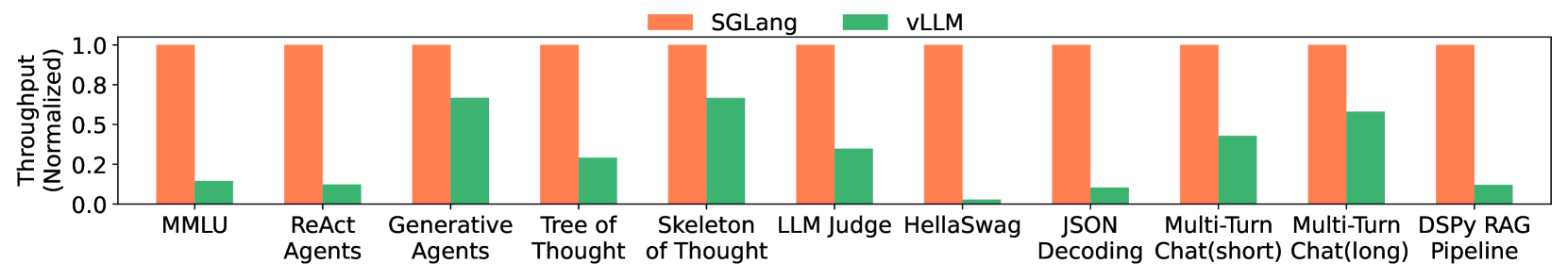
Figure 7: Normalized throughput on Mixtral-8x7B models with tensor parallelism. Higher is better.
Results on larger models with tensor parallelism. We run larger models, Mixtral-8x7B and Llama-70B, with tensor parallelism on the same set of benchmarks and report the results in Fig. 7 and Fig. 12 (Appendix). The speedup on larger models shows a trend similar to that observed on smaller models, indicating that our optimization generalizes well to larger models. We omit Guidance and LMQL here because they lack efficient implementations of tensor parallelism.
Results on multi-modal models. SGLang has native support for multi-modal models with the image and video primitives. The optimizations in this paper are compatible with multi-modal models. For RadixAttention, we compute the hash of the input images and use it as the key in the radix tree, allowing us to reuse the KV cache of the image tokens from the same image. We run LLaVA-v1.5-7B (image) on llava-bench-in-the-wild and LLaVA-NeXT-34B (video) on ActivityNet. Because these models are not well supported by other baseline systems, we use the model authors’ original implementation in Hugging Face Transformers as the baseline. As shown in Table 2, SGLang provides throughput up to $6×$ higher on these benchmarks. In llava-bench-in-the-wild, there are multiple questions about the same image, and SGLang runtime reuses the KV cache in this case.
Table 2: Throughput comparison on multi-modal LLaVA image and video models.
| Author’s original implementation | 0.18 image/s | 0.02 frame/s |
| --- | --- | --- |
| SGLang | 1.15 image/s | 0.10 frame/s |
Production deployment. SGLang has been deployed in Chatbot Arena chiang2024chatbot to serve open-weight models. Due to low traffic for some models, only one SGLang worker serves each. After one month, we observed a 52.4% RadixAttention cache hit rate for LLaVA-Next-34B liu2024llavanext and 74.1% for Vicuna-33B vicuna2023 . Cache hits come from common system messages, frequently reused example images, and multi-turn chat histories. This reduces first-token latency by an average of $1.7×$ for Vicuna-33B.
Results on API models. We test a prompt that extracts three fields from a Wikipedia page using OpenAI’s GPT-3.5 model. By using few-shot prompting, the accuracy of API speculative execution is high, and it reduces the cost of input tokens by about threefold due to the extraction of three fields.
<details>
<summary>x8.png Details</summary>
### Visual Description
# Technical Data Extraction: Performance Metrics Analysis
This document contains a detailed extraction of data from three performance charts labeled (a), (b), and (c).
---
## Chart (a): Impact of Cache Hit Rate on Batch Size and Throughput
### Metadata
- **X-Axis:** Cache Hit Rate (%) [Range: 0 to 100]
- **Primary Y-Axis (Left, Green):** Batch Size [Range: 20 to 40+]
- **Secondary Y-Axis (Right, Orange):** Throughput (tokens / s) [Range: 0.4k to 1.2k]
- **Legend Location:** Top Left
### Data Series Trends
1. **Batch Size (Green Line):** Shows a consistent upward slope. The growth rate increases slightly as the cache hit rate exceeds 60%.
2. **Throughput (Orange Line):** Shows a consistent upward slope, closely tracking the batch size. It exhibits exponential-like growth towards the 100% hit rate mark.
### Key Data Points (Approximate)
| Cache Hit Rate (%) | Batch Size (Green) | Throughput (Orange) |
| :--- | :--- | :--- |
| 0 | 20 | ~0.4k |
| 20 | ~23 | ~0.45k |
| 40 | ~26 | ~0.5k |
| 60 | ~32 | ~0.65k |
| 80 | ~37 | ~0.85k |
| 100 | ~48 | ~1.15k |
---
## Chart (b): Impact of Cache Hit Rate on Latency
### Metadata
- **X-Axis:** Cache Hit Rate (%) [Range: 0 to 100]
- **Primary Y-Axis (Left, Red):** Total Latency (s) [Range: 200 to 400+]
- **Secondary Y-Axis (Right, Blue):** First Token Latency (s) [Range: 10 to 20+]
- **Legend Location:** Top Right
### Data Series Trends
1. **Total Latency (Red Line):** Shows a steady, linear downward trend as the cache hit rate increases, dropping from over 400s to approximately 120s.
2. **First Token Latency (Blue Line):** Shows a sharp initial drop between 0% and 10% hit rate, followed by a gradual, fluctuating decline toward the 100% mark.
### Key Data Points (Approximate)
| Cache Hit Rate (%) | Total Latency (Red) | First Token Latency (Blue) |
| :--- | :--- | :--- |
| 0 | ~430s | ~25s |
| 20 | ~350s | ~8s |
| 40 | ~310s | ~8s |
| 60 | ~230s | ~7s |
| 80 | ~180s | ~5s |
| 100 | ~120s | ~3s |
---
## Chart (c): Throughput Ablation Study across Workloads
### Metadata
- **Y-Axis:** Throughput (Normalized) [Range: 0.00 to 1.00]
- **X-Axis Categories:** LLM Judge, Tree of Thought, MMLU, Multi-Turn Chat (short)
- **Legend (Top):**
* **Light Gray:** No Cache
* **Dark Gray:** No Tree Structure
* **Dark Green:** FCFS Schedule
* **Medium Green:** Random Schedule
* **Dark Blue:** No Frontend Parallelism
* **Light Blue:** No Frontend Hint
* **Orange:** Full Optimization
### Data Table (Normalized Throughput)
| Configuration | LLM Judge | Tree of Thought | MMLU | Multi-Turn Chat |
| :--- | :---: | :---: | :---: | :---: |
| **No Cache** (Light Gray) | ~0.40 | ~0.28 | ~0.18 | ~0.53 |
| **No Tree Structure** (Dark Gray) | ~0.45 | ~0.35 | ~0.60 | ~0.88 |
| **FCFS Schedule** (Dark Green) | ~0.15 | ~0.35 | ~0.98 | ~0.53 |
| **Random Schedule** (Med Green) | ~0.50 | ~0.45 | ~0.98 | ~0.68 |
| **No Frontend Parallelism** (Dark Blue) | ~0.52 | ~0.35 | ~0.98 | ~0.95 |
| **No Frontend Hint** (Light Blue) | ~0.50 | ~0.88 | ~0.98 | ~0.98 |
| **Full Optimization** (Orange) | **1.00** | **1.00** | **1.00** | **1.00** |
### Key Observations
* **Full Optimization** consistently achieves the highest throughput (1.00) across all test cases.
* **Tree of Thought** is most sensitive to the "No Frontend Hint" and "No Cache" configurations.
* **MMLU** shows significant performance degradation specifically when "No Cache" is used, but remains high for most other configurations.
* **LLM Judge** shows the worst performance under the "FCFS Schedule" compared to other workloads.
</details>
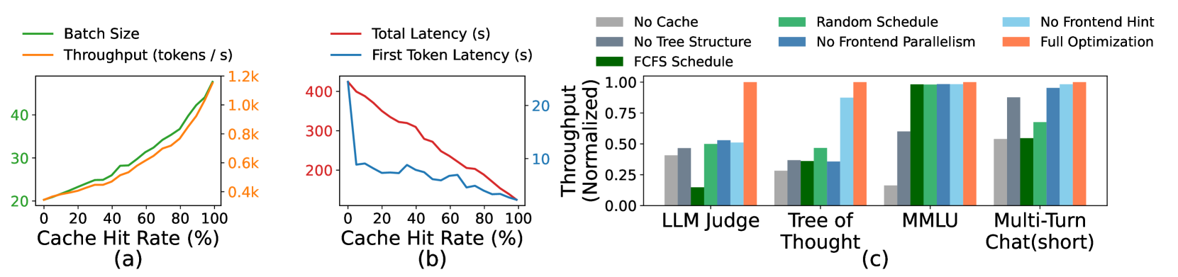
Figure 8: (a)(b) Cache hit rate ablation study. (c) RadixAttention ablation study.
6.3 Ablation Study
Cache hit rate vs. latency/throughput. Fig. 8 (a)(b) shows the relationship between cache hit rate and performance metrics (first token latency, total latency, batch size, and throughput) on the tree-of-thought benchmark. The figure is obtained by partially disabling matched tokens at runtime. It shows that a higher cache hit rate leads to a larger batch size, higher throughput, and lower latency.
Effectiveness of RadixAttention. We test the effectiveness of RadixAttention and its components on several representative benchmarks. As shown in Fig. 8 (c), "No Cache" means not using any cache, "No Tree-Structure" means using a simple table-based cache instead of a tree-structured cache, "FCFS Schedule" means using a first-come-first-serve policy instead of our cache-aware scheduling, "Random Schedule" means using a random order to schedule requests, "No Frontend Parallelism" means disabling parallelism in the interpreter, "No Frontend Hint" means disabling sending the fork hints from the interpreters, and "Full optimizations" means we turn on all optimizations. The experimental results show that each of these components is required to achieve the best performance. Disabling parallelism and hints from the frontend interpreter also results in suboptimal runtime performance, highlighting the importance of co-designing the frontend language and runtime.
Overhead of RadixAttention. We test the overhead of RadixAttention on a benchmark without any KV cache reuse opportunities. The benchmark measures throughput on the ShareGPT dataset. It takes 74.3 seconds to run 100 requests; however, the time used for managing the RadixAttention data structures is only 0.2 seconds, which is a negligible overhead of less than 0.3%. This is because the complexity of tree operations is linear and small. Thus, we can turn on RadixAttention by default.
Effectiveness of the compressed finite state machine. We test the effectiveness of the compressed finite state machine and its components on the JSON decoding benchmark. Experimental results show that the compressed finite state machine increases the throughput by $1.6×$ because it can decode multiple tokens at once. In addition, we need to preprocess the state machine and reuse it for a batch of requests. Otherwise, redoing the preprocessing for each request makes the throughput $2.4×$ lower.
7 Related Work
Various works have explored the reuse of the KV cache, and many of them are concurrent with our work. Uniquely, our RadixAttention first proposes treating the KV cache as a tree-based LRU cache. It is the first solution that supports multi-level sharing, cache-aware scheduling, frontend-runtime co-scheduling, and distributed cases. vLLM kwon2023vllm and ChunkedAttention ye2024chunkattention explore some simple reuse cases (e.g., system prompt sharing) but do not cover multi-level tree-structured sharing or LRU caching. PromptCache gim2023prompt proposes the modular reuse of the KV cache beyond the prefix but can impact accuracy by up to a 43% drop. HydraGen juravsky2024hydragen , FlashInfer flashinfer , and ChunkedAttention ye2024chunkattention focus on CUDA kernel optimizations and do not include the concept of an LRU cache. API Serve abhyankar2024apiserve and LLM-SQL liu2024optimizing study KV cache reuse for specific applications such as interleaving with external API calls and relational databases, but they do not have our radix tree or cache-aware scheduling.
Several LLM programming and agent frameworks exist, such as Guidance guidance , LMQL beurer2023lmql , DSPy khattab2023dspy , LangChain langchain , AutoGen wu2023autogen , and LLM Compiler kim2023llm . Guidance and LMQL are most similar to SGLang, and we compare them in Sec. 2. Our innovation lies in novel runtime optimizations for accelerating the proposed programming model. SGLang is compatible with other frameworks and can accelerate them (e.g., the DSPy example in our evaluation). Additionally, SGLang is compatible with many other common inference optimizations yu2022orca ; pope2023efficiently ; aminabadi2022deepspeed ; kwon2023vllm ; flashinfer ; dao2022flashattention ; lin2023awq ; hooper2024kvquant ; kang2024gear ; liu2024kivi ; liu2024scissorhands ; ge2023model .
8 Future Directions and Conclusion
Future directions. Despite the progress made with SGLang, several limitations remain that reveal promising directions for future research. These include extending SGLang to support additional output modalities, adapting RadixAttention to operate across multiple levels of the memory hierarchy (e.g., DRAM, Disk) sheng2023flexgen , enabling fuzzy semantic matching within RadixAttention, providing higher-level primitives atop SGLang, fixing starvation in cache-aware scheduling sheng2023fairness , and enhancing the SGLang compiler to perform advanced static optimizations such as scheduling and memory planning.
Conclusion. We introduce SGLang, a framework for efficient programming and executing structured language model programs. SGLang significantly improves the throughput and latency of complex LM programs through novel optimizations like RadixAttention, compressed finite state machines, and a language interpreter. It is a valuable tool for developing advanced prompting techniques and agent workflows. The source code is publicly available.
Acknowledgement
This project is supported by the Stanford Center for Automated Reasoning and gifts from Astronomer, Google, IBM, Intel, Lacework, Microsoft, Mohamed Bin Zayed University of Artificial Intelligence, Nexla, Samsung SDS, Uber, and VMware. Lianmin Zheng is supported by a Meta Ph.D. Fellowship. We thank Yuanhan Zhang and Bo Li for the LLaVA-NeXT (video) support.
References
- [1] Reyna Abhyankar, Zijian He, Vikranth Srivatsa, Hao Zhang, and Yiying Zhang. Apiserve: Efficient api support for large-language model inferencing. arXiv preprint arXiv:2402.01869, 2024.
- [2] Jean-Baptiste Alayrac, Jeff Donahue, Pauline Luc, Antoine Miech, Iain Barr, Yana Hasson, Karel Lenc, Arthur Mensch, Katherine Millican, Malcolm Reynolds, et al. Flamingo: a visual language model for few-shot learning. Advances in Neural Information Processing Systems, 35:23716–23736, 2022.
- [3] Reza Yazdani Aminabadi, Samyam Rajbhandari, Ammar Ahmad Awan, Cheng Li, Du Li, Elton Zheng, Olatunji Ruwase, Shaden Smith, Minjia Zhang, Jeff Rasley, et al. Deepspeed-inference: enabling efficient inference of transformer models at unprecedented scale. In SC22: International Conference for High Performance Computing, Networking, Storage and Analysis, pages 1–15. IEEE, 2022.
- [4] Luca Beurer-Kellner, Marc Fischer, and Martin Vechev. Prompting is programming: A query language for large language models. Proceedings of the ACM on Programming Languages, 7(PLDI):1946–1969, 2023.
- [5] Tom Brown, Benjamin Mann, Nick Ryder, Melanie Subbiah, Jared D Kaplan, Prafulla Dhariwal, Arvind Neelakantan, Pranav Shyam, Girish Sastry, Amanda Askell, et al. Language models are few-shot learners. Advances in neural information processing systems, 33:1877–1901, 2020.
- [6] Sébastien Bubeck, Varun Chandrasekaran, Ronen Eldan, Johannes Gehrke, Eric Horvitz, Ece Kamar, Peter Lee, Yin Tat Lee, Yuanzhi Li, Scott Lundberg, et al. Sparks of artificial general intelligence: Early experiments with gpt-4. arXiv preprint arXiv:2303.12712, 2023.
- [7] Wei-Lin Chiang, Zhuohan Li, Zi Lin, Ying Sheng, Zhanghao Wu, Hao Zhang, Lianmin Zheng, Siyuan Zhuang, Yonghao Zhuang, Joseph E. Gonzalez, Ion Stoica, and Eric P. Xing. Vicuna: An open-source chatbot impressing gpt-4 with 90%* chatgpt quality, March 2023.
- [8] Wei-Lin Chiang, Lianmin Zheng, Ying Sheng, Anastasios Nikolas Angelopoulos, Tianle Li, Dacheng Li, Hao Zhang, Banghua Zhu, Michael Jordan, Joseph E Gonzalez, et al. Chatbot arena: An open platform for evaluating llms by human preference. arXiv preprint arXiv:2403.04132, 2024.
- [9] Aakanksha Chowdhery, Sharan Narang, Jacob Devlin, Maarten Bosma, Gaurav Mishra, Adam Roberts, Paul Barham, Hyung Won Chung, Charles Sutton, Sebastian Gehrmann, et al. Palm: Scaling language modeling with pathways. arXiv preprint arXiv:2204.02311, 2022.
- [10] Tri Dao, Dan Fu, Stefano Ermon, Atri Rudra, and Christopher Ré. Flashattention: Fast and memory-efficient exact attention with io-awareness. Advances in Neural Information Processing Systems, 35:16344–16359, 2022.
- [11] Suyu Ge, Yunan Zhang, Liyuan Liu, Minjia Zhang, Jiawei Han, and Jianfeng Gao. Model tells you what to discard: Adaptive kv cache compression for llms. In The Twelfth International Conference on Learning Representations, 2023.
- [12] In Gim, Guojun Chen, Seung-seob Lee, Nikhil Sarda, Anurag Khandelwal, and Lin Zhong. Prompt cache: Modular attention reuse for low-latency inference. arXiv preprint arXiv:2311.04934, 2023.
- [13] Guidance AI. A guidance language for controlling large language models. https://github.com/guidance-ai/guidance. Accessed: 2023-11.
- [14] Dan Hendrycks, Collin Burns, Steven Basart, Andy Zou, Mantas Mazeika, Dawn Song, and Jacob Steinhardt. Measuring massive multitask language understanding. In International Conference on Learning Representations, 2020.
- [15] Coleman Hooper, Sehoon Kim, Hiva Mohammadzadeh, Michael W Mahoney, Yakun Sophia Shao, Kurt Keutzer, and Amir Gholami. Kvquant: Towards 10 million context length llm inference with kv cache quantization. arXiv preprint arXiv:2401.18079, 2024.
- [16] Hugging Face. Text generation inference. https://github.com/huggingface/text-generation-inference. Accessed: 2023-11.
- [17] Albert Q Jiang, Alexandre Sablayrolles, Antoine Roux, Arthur Mensch, Blanche Savary, Chris Bamford, Devendra Singh Chaplot, Diego de las Casas, Emma Bou Hanna, Florian Bressand, et al. Mixtral of experts. arXiv preprint arXiv:2401.04088, 2024.
- [18] Jordan Juravsky, Bradley Brown, Ryan Ehrlich, Daniel Y Fu, Christopher Ré, and Azalia Mirhoseini. Hydragen: High-throughput llm inference with shared prefixes. arXiv preprint arXiv:2402.05099, 2024.
- [19] Hao Kang, Qingru Zhang, Souvik Kundu, Geonhwa Jeong, Zaoxing Liu, Tushar Krishna, and Tuo Zhao. Gear: An efficient kv cache compression recipefor near-lossless generative inference of llm. arXiv preprint arXiv:2403.05527, 2024.
- [20] Omar Khattab, Arnav Singhvi, Paridhi Maheshwari, Zhiyuan Zhang, Keshav Santhanam, Sri Vardhamanan, Saiful Haq, Ashutosh Sharma, Thomas T. Joshi, Hanna Moazam, Heather Miller, Matei Zaharia, and Christopher Potts. Dspy: Compiling declarative language model calls into self-improving pipelines. arXiv preprint arXiv:2310.03714, 2023.
- [21] Sehoon Kim, Suhong Moon, Ryan Tabrizi, Nicholas Lee, Michael W Mahoney, Kurt Keutzer, and Amir Gholami. An llm compiler for parallel function calling. arXiv preprint arXiv:2312.04511, 2023.
- [22] Michael Kuchnik, Virginia Smith, and George Amvrosiadis. Validating large language models with relm. Proceedings of Machine Learning and Systems, 5, 2023.
- [23] Woosuk Kwon, Zhuohan Li, Siyuan Zhuang, Ying Sheng, Lianmin Zheng, Cody Hao Yu, Joseph Gonzalez, Hao Zhang, and Ion Stoica. Efficient memory management for large language model serving with pagedattention. In Proceedings of the 29th Symposium on Operating Systems Principles, pages 611–626, 2023.
- [24] LangChain AI. Langchain. https://github.com/langchain-ai/langchain. Accessed: 2023-11.
- [25] Yujia Li, David Choi, Junyoung Chung, Nate Kushman, Julian Schrittwieser, Rémi Leblond, Tom Eccles, James Keeling, Felix Gimeno, Agustin Dal Lago, et al. Competition-level code generation with alphacode. Science, 378(6624):1092–1097, 2022.
- [26] Ji Lin, Jiaming Tang, Haotian Tang, Shang Yang, Xingyu Dang, and Song Han. Awq: Activation-aware weight quantization for llm compression and acceleration. arXiv preprint arXiv:2306.00978, 2023.
- [27] Haotian Liu, Chunyuan Li, Yuheng Li, and Yong Jae Lee. Improved baselines with visual instruction tuning. arXiv preprint arXiv:2310.03744, 2023.
- [28] Haotian Liu, Chunyuan Li, Yuheng Li, Bo Li, Yuanhan Zhang, Sheng Shen, and Yong Jae Lee. Llava-next: Improved reasoning, ocr, and world knowledge, January 2024.
- [29] Shu Liu, Asim Biswal, Audrey Cheng, Xiangxi Mo, Shiyi Cao, Joseph E Gonzalez, Ion Stoica, and Matei Zaharia. Optimizing llm queries in relational workloads. arXiv preprint arXiv:2403.05821, 2024.
- [30] Xiaoxia Liu, Jingyi Wang, Jun Sun, Xiaohan Yuan, Guoliang Dong, Peng Di, Wenhai Wang, and Dongxia Wang. Prompting frameworks for large language models: A survey. arXiv preprint arXiv:2311.12785, 2023.
- [31] Zichang Liu, Aditya Desai, Fangshuo Liao, Weitao Wang, Victor Xie, Zhaozhuo Xu, Anastasios Kyrillidis, and Anshumali Shrivastava. Scissorhands: Exploiting the persistence of importance hypothesis for llm kv cache compression at test time. Advances in Neural Information Processing Systems, 36, 2024.
- [32] Zirui Liu, Jiayi Yuan, Hongye Jin, Shaochen Zhong, Zhaozhuo Xu, Vladimir Braverman, Beidi Chen, and Xia Hu. Kivi: A tuning-free asymmetric 2bit quantization for kv cache. arXiv preprint arXiv:2402.02750, 2024.
- [33] Xuefei Ning, Zinan Lin, Zixuan Zhou, Zifu Wang, Huazhong Yang, and Yu Wang. Skeleton-of-thought: Prompting LLMs for efficient parallel generation. In The Twelfth International Conference on Learning Representations, 2024.
- [34] NVIDIA. Tensorrt-llm. https://github.com/NVIDIA/TensorRT-LLM. Accessed: 2023-11.
- [35] OpenAI. Gpt-4 technical report, 2023.
- [36] Joon Sung Park, Joseph C. O’Brien, Carrie J. Cai, Meredith Ringel Morris, Percy Liang, and Michael S. Bernstein. Generative agents: Interactive simulacra of human behavior. In In the 36th Annual ACM Symposium on User Interface Software and Technology (UIST ’23), UIST ’23, New York, NY, USA, 2023. Association for Computing Machinery.
- [37] Adam Paszke, Sam Gross, Francisco Massa, Adam Lerer, James Bradbury, Gregory Chanan, Trevor Killeen, Zeming Lin, Natalia Gimelshein, Luca Antiga, et al. Pytorch: An imperative style, high-performance deep learning library. Advances in neural information processing systems, 32, 2019.
- [38] Shishir G. Patil, Tianjun Zhang, Xin Wang, and Joseph E. Gonzalez. Gorilla: Large language model connected with massive apis. arXiv preprint arXiv:2305.15334, 2023.
- [39] Reiner Pope, Sholto Douglas, Aakanksha Chowdhery, Jacob Devlin, James Bradbury, Jonathan Heek, Kefan Xiao, Shivani Agrawal, and Jeff Dean. Efficiently scaling transformer inference. Proceedings of Machine Learning and Systems, 5, 2023.
- [40] Swarnadeep Saha, Omer Levy, Asli Celikyilmaz, Mohit Bansal, Jason Weston, and Xian Li. Branch-solve-merge improves large language model evaluation and generation. arXiv preprint arXiv:2310.15123, 2023.
- [41] Timo Schick, Jane Dwivedi-Yu, Roberto Dessì, Roberta Raileanu, Maria Lomeli, Luke Zettlemoyer, Nicola Cancedda, and Thomas Scialom. Toolformer: Language models can teach themselves to use tools. arXiv preprint arXiv:2302.04761, 2023.
- [42] Ying Sheng, Shiyi Cao, Dacheng Li, Banghua Zhu, Zhuohan Li, Danyang Zhuo, Joseph E Gonzalez, and Ion Stoica. Fairness in serving large language models. arXiv preprint arXiv:2401.00588, 2023.
- [43] Ying Sheng, Lianmin Zheng, Binhang Yuan, Zhuohan Li, Max Ryabinin, Beidi Chen, Percy Liang, Christopher Ré, Ion Stoica, and Ce Zhang. Flexgen: high-throughput generative inference of large language models with a single gpu. In International Conference on Machine Learning, pages 31094–31116. PMLR, 2023.
- [44] Mohammad Shoeybi, Mostofa Patwary, Raul Puri, Patrick LeGresley, Jared Casper, and Bryan Catanzaro. Megatron-lm: Training multi-billion parameter language models using model parallelism. arXiv preprint arXiv:1909.08053, 2019.
- [45] Vikranth Srivatsa, Zijian He, Reyna Abhyankar, Dongming Li, and Yiying Zhang. Preble: Efficient distributed prompt scheduling for llm serving. 2024.
- [46] Theodore Sumers, Shunyu Yao, Karthik Narasimhan, and Thomas Griffiths. Cognitive architectures for language agents. Transactions on Machine Learning Research, 2023.
- [47] Gemini Team, Rohan Anil, Sebastian Borgeaud, Yonghui Wu, Jean-Baptiste Alayrac, Jiahui Yu, Radu Soricut, Johan Schalkwyk, Andrew M Dai, Anja Hauth, et al. Gemini: a family of highly capable multimodal models. arXiv preprint arXiv:2312.11805, 2023.
- [48] Philippe Tillet, Hsiang-Tsung Kung, and David Cox. Triton: an intermediate language and compiler for tiled neural network computations. In Proceedings of the 3rd ACM SIGPLAN International Workshop on Machine Learning and Programming Languages, pages 10–19, 2019.
- [49] Hugo Touvron, Louis Martin, Kevin Stone, Peter Albert, Amjad Almahairi, Yasmine Babaei, Nikolay Bashlykov, Soumya Batra, Prajjwal Bhargava, Shruti Bhosale, et al. Llama 2: Open foundation and fine-tuned chat models. arXiv preprint arXiv:2307.09288, 2023.
- [50] Vivien Tran-Thien. Fast, high-fidelity llm decoding with regex constraints, 2024.
- [51] Ashish Vaswani, Noam Shazeer, Niki Parmar, Jakob Uszkoreit, Llion Jones, Aidan N Gomez, Łukasz Kaiser, and Illia Polosukhin. Attention is all you need. Advances in neural information processing systems, 30, 2017.
- [52] Guanzhi Wang, Yuqi Xie, Yunfan Jiang, Ajay Mandlekar, Chaowei Xiao, Yuke Zhu, Linxi Fan, and Anima Anandkumar. Voyager: An open-ended embodied agent with large language models. arXiv preprint arXiv: Arxiv-2305.16291, 2023.
- [53] Xuezhi Wang, Jason Wei, Dale Schuurmans, Quoc V Le, Ed H Chi, Sharan Narang, Aakanksha Chowdhery, and Denny Zhou. Self-consistency improves chain of thought reasoning in language models. In The Eleventh International Conference on Learning Representations, 2022.
- [54] Brandon T Willard and Rémi Louf. Efficient guided generation for large language models. arXiv e-prints, pages arXiv–2307, 2023.
- [55] Qingyun Wu, Gagan Bansal, Jieyu Zhang, Yiran Wu, Shaokun Zhang, Erkang Zhu, Beibin Li, Li Jiang, Xiaoyun Zhang, and Chi Wang. Autogen: Enabling next-gen llm applications via multi-agent conversation framework. arXiv preprint arXiv:2308.08155, 2023.
- [56] Shunyu Yao, Dian Yu, Jeffrey Zhao, Izhak Shafran, Thomas L Griffiths, Yuan Cao, and Karthik Narasimhan. Tree of thoughts: Deliberate problem solving with large language models. arXiv preprint arXiv:2305.10601, 2023.
- [57] Shunyu Yao, Jeffrey Zhao, Dian Yu, Nan Du, Izhak Shafran, Karthik R Narasimhan, and Yuan Cao. React: Synergizing reasoning and acting in language models. In The Eleventh International Conference on Learning Representations, 2022.
- [58] Lu Ye, Ze Tao, Yong Huang, and Yang Li. Chunkattention: Efficient self-attention with prefix-aware kv cache and two-phase partition. arXiv preprint arXiv:2402.15220, 2024.
- [59] Zihao Ye, Lequn Chen, Ruihang Lai, Yilong Zhao, Size Zheng, Junru Shao, Bohan Hou, Hongyi Jin, Yifei Zuo, Liangsheng Yin, Tianqi Chen, and Luis Ceze. Accelerating self-attentions for llm serving with flashinfer, February 2024.
- [60] Gyeong-In Yu, Joo Seong Jeong, Geon-Woo Kim, Soojeong Kim, and Byung-Gon Chun. Orca: A distributed serving system for $\{$ Transformer-Based $\}$ generative models. In 16th USENIX Symposium on Operating Systems Design and Implementation (OSDI 22), pages 521–538, 2022.
- [61] Rowan Zellers, Ari Holtzman, Yonatan Bisk, Ali Farhadi, and Yejin Choi. Hellaswag: Can a machine really finish your sentence? In Proceedings of the 57th Annual Meeting of the Association for Computational Linguistics, pages 4791–4800, 2019.
- [62] Yuanhan Zhang, Bo Li, haotian Liu, Yong jae Lee, Liangke Gui, Di Fu, Jiashi Feng, Ziwei Liu, and Chunyuan Li. Llava-next: A strong zero-shot video understanding model, April 2024.
Appendix A Additional Details on RadixAttention
A.1 Background on the KV Cache
Most LLMs in use today, such as GPT-3 [5], PaLM [9], and LLaMA [49], are based on the autoregressive Transformer architecture [51]. These models predict the probability of the next token in a sequence based on the preceding tokens. During inference, the model first processes a sequence of input tokens through a forward pass (this process is called "prefill"). It then sequentially decodes output tokens, with each token depending on prior tokens (this process is called "decoding"). We refer to the process of taking a sequence of input tokens and generating a sequence of output tokens as a single-generation call. Throughout this process, each token generates some intermediate tensors, which are used for decoding further tokens. These intermediate tensors, known as the "KV Cache," are named for the key-value pairs in the self-attention mechanism. An important observation when discussing optimizations in this paper is that the computation of the KV cache only depends on all previous tokens, so different sequences with the same prefix can reuse the KV cache of the prefix tokens and avoid redundant computation.
Often in LLM programs, multiple text segments and generation calls are appended to a single prompt. Caching the computed KV cache for previous tokens across multiple chained calls can reduce redundant computation. This optimization, however, is neither free nor trivial, as it requires additional storage and more complex memory management. In addition, it is common in LLM programs to generate multiple outputs from a single prompt or to fork a new prompt from the current state [25]. Basic prefix sharing has been investigated in vLLM [23]. More advanced sharing patterns like irregular tree-structured sharing can also be employed. Fig. 9 shows four typical patterns of KV cache sharing across multiple calls; none of the existing systems can automatically handle all of them. On the contrary, our RadixAttention in Sec. 3 can handle all of them automatically at runtime.
<details>
<summary>x9.png Details</summary>
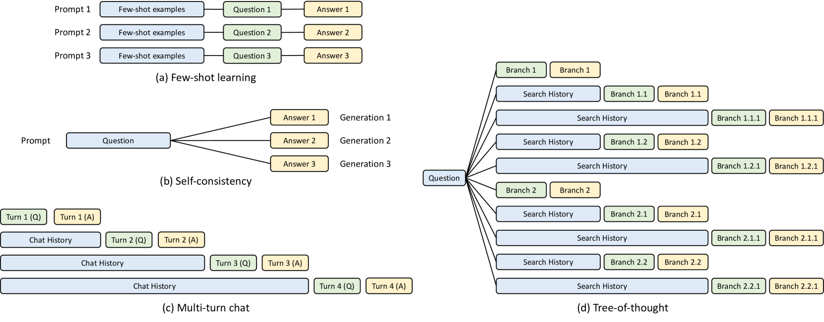
### Visual Description
# Technical Diagram Analysis: Prompting and Reasoning Strategies
This image illustrates four distinct methodologies for structuring prompts and managing Large Language Model (LLM) outputs. The diagram is divided into four quadrants, labeled (a) through (d).
## Color Coding Legend
Across all diagrams, a consistent color scheme is used to denote functional components:
* **Light Blue:** Context, Examples, or History (Input data).
* **Light Green:** The specific Question or Branching logic.
* **Light Yellow:** The generated Answer or Result.
---
## (a) Few-shot learning
This section demonstrates a linear, repetitive structure where the model is provided with examples before the final task.
* **Structure:** Three parallel horizontal tracks labeled **Prompt 1**, **Prompt 2**, and **Prompt 3**.
* **Flow:** Each track follows a sequential flow: `[Few-shot examples]` $\rightarrow$ `[Question X]` $\rightarrow$ `[Answer X]`.
* **Components:**
* **Prompt 1:** Few-shot examples $\rightarrow$ Question 1 $\rightarrow$ Answer 1
* **Prompt 2:** Few-shot examples $\rightarrow$ Question 2 $\rightarrow$ Answer 2
* **Prompt 3:** Few-shot examples $\rightarrow$ Question 3 $\rightarrow$ Answer 3
---
## (b) Self-consistency
This section illustrates a one-to-many relationship where a single prompt generates multiple independent outputs to find a consensus.
* **Structure:** A single input branching into three parallel outputs.
* **Flow:** A central **Prompt** containing a `[Question]` branches out to three separate generations.
* **Components:**
* **Generation 1:** Answer 1
* **Generation 2:** Answer 2
* **Generation 3:** Answer 3
---
## (c) Multi-turn chat
This section depicts the cumulative nature of conversational history over four successive turns.
* **Structure:** A staggered, descending stack representing the growth of context over time.
* **Flow:**
* **Turn 1:** `[Turn 1 (Q)]` followed by `[Turn 1 (A)]`.
* **Turn 2:** `[Chat History]` (containing Turn 1) + `[Turn 2 (Q)]` $\rightarrow$ `[Turn 2 (A)]`.
* **Turn 3:** `[Chat History]` (containing Turns 1-2) + `[Turn 3 (Q)]` $\rightarrow$ `[Turn 3 (A)]`.
* **Turn 4:** `[Chat History]` (containing Turns 1-3) + `[Turn 4 (Q)]` $\rightarrow$ `[Turn 4 (A)]`.
* **Trend:** The `Chat History` block (Blue) grows significantly longer with each subsequent turn.
---
## (d) Tree-of-thought
This section shows a complex, hierarchical branching structure used for exploring multiple reasoning paths.
* **Structure:** A root node branching into primary, secondary, and tertiary levels.
* **Flow:** Starts with a single `[Question]` node on the left, which branches into multiple paths.
* **Components and Hierarchy:**
* **Level 1 (Primary Branches):**
* **Branch 1:** Leads to a `Branch 1` answer.
* **Branch 2:** Leads to a `Branch 2` answer.
* **Level 2 (Secondary Branches):**
* From the root, paths include `[Search History]` leading to `Branch 1.1` and `Branch 1.2`.
* From the root, paths include `[Search History]` leading to `Branch 2.1` and `Branch 2.2`.
* **Level 3 (Tertiary Branches):**
* Extended `[Search History]` blocks lead to deeper sub-branches: `Branch 1.1.1`, `Branch 1.2.1`, `Branch 2.1.1`, and `Branch 2.2.1`.
* **Key Observation:** Each deeper level of the tree incorporates a longer `Search History` (Blue) block to maintain the context of the reasoning path.
</details>
Figure 9: KV cache sharing examples. Blue boxes represent shareable prompt parts, green boxes indicate non-shareable parts and yellow boxes mark non-shareable model outputs. Shareable elements include few-shot learning examples, questions in self-consistency [53], chat history in multi-turn chat, and search history in tree-of-thought [56].
Algorithm 1 Cache-Aware Scheduling for RadixAttention with Continuous Batching.
The radix tree $T$ , the memory pool $P$ , the current running batch $B$ , the waiting queue $Q$ .
Finished requests and updated system state.
// Get all requests from the waiting queue
$requests← Q.\text{get\_all\_requests}()$
// Search for the prefix matching for all waiting requests
for $req∈ requests$ do
$req.prefix\_node,req.prefix\_len←$ $T.\text{match\_prefix}(req.input\_tokens)$
end for
// Sort the requests according to the matched prefix lenghts
$requests.\text{sort}()$
// Select requests for the next batch
$available\_size← T.\text{evictable\_size}()+P.\text{available\_size}()$
$current\_size← 0$
$new\_batch←[]$
for $req∈ requests$ do
if $req.\text{size}()+current\_size<available\_size$ then
$new\_batch.\text{append}(req)$
$delta← T.\text{increase\_ref\_counter}(req.prefix\_node)$
$available\_size← available\_size+delta$
end if
end for
$Q.\text{remove\_requests}(new\_batch)$
// Insert requests into the current running batch
$B.\text{merge}(new\_batch)$
// Allocate new memory and do eviction if necessary
$needed\_size← B.\text{needed\_size}()$
$success,buffer← P.\text{alloc}(needed\_size)$
if not $success$ then
$T.\text{evict}(needed\_size)$
$success,buffer← P.\text{alloc}(needed\_size)$
end if
$B.\text{run}(buffer)$
// Process finished requests
$finished\_requests← B.\text{drop\_finished\_requests}()$
for $req∈ finished\_requests$ do
$T.\text{decrease\_ref\_counter}(req.prefix\_node)$
$T.\text{insert}(req)$
end for
return $finished\_requests$
A.2 Pseudocode for Cache-Aware Scheduling
Alg. 1 shows the pseudocode of cache-aware scheduling for RadixAttention with continuous batching.
A.3 Proof of the Theorem 3.1
See 3.1
* Proof*
First, we show that the depth-first search (DFS) order achieves an optimal cache hit rate. Let $R$ denote the set of requests in the batch, and $T$ denote the radix tree built from $R$ . For each edge $e$ of $T$ , the KV cache associated with $e$ needs to be computed at least once. Let $|e|$ denote the size of the KV cache associated with $e$ . Let $C$ denote the computational complexity of the KV cache for $R$ . We obtain the lower bound
$$
C\geq\sum_{e\in\text{edges}(T)}|e|.
$$ Consider we visit the radix tree $T$ in DFS order. For each edge $e$ of $T$ , the first time we compute the KV cache associated with $e$ , we will then compute the whole subtree of $e$ . During the computation of the subtree of $e$ , the edge $e$ will be continuously hit, so no additional computation will happen. After finishing the computation for the subtree rooted at $e$ , the edge $e$ will not be visited again. Notice that, with a cache size $≥$ the maximum request length, which equals the longest path in the radix tree $T$ , edge $e$ will not be evicted during the computation of its subtree, since the common prefix including $e$ of the subtree will be continuously hit. Therefore, the KV cache associated with each edge $e$ will be computed only once. Thus, we achieve the lower bound
$$
C=\sum_{e\in\text{edges}(T)}|e|.
$$ The cache hit rate, defined as
$$
\frac{\sum_{r\in R}\text{number of cached prefill tokens in $r$}}{\sum_{r\in R%
}\text{number of prefill tokens in $r$}},
$$
equals $1-\frac{C}{\sum_{r∈ R}\text{number of prefill tokens}}$ , reaches its upper bound, delivering optimality. Next, we show that the longest-shared-prefix-first order is equivalent to a DFS order by induction.
- (Base) In the beginning, since there is nothing cached, a random request that corresponds to a node $x$ in $T$ will be processed. All requests that correspond to the nodes $\{v_{1},...,v_{n}\}$ on the path from the root to $x$ do not need a recomputation. The computation complexity for requests corresponding to the nodes $\{v_{1},...,v_{n},x\}$ is aligned with a valid DFS. The path from the root to $x$ is cached.
- (Induction) Assume we just visited a node $y$ in $T$ , and the visited nodes align with a DFS order. Let $P$ denote the path from the root to $y$ . Then each node that has not been visited has the lowest common ancestor with the visited nodes on $P$ . Since nodes on $P$ are cached, a node $z$ that has not been visited with the lowest common ancestor on $P$ will have the longest shared prefix. The longest-shared-prefix-first order will select $z$ , which is a valid DFS order. The path from the root to $z$ will be cached because it is the most recent.
∎
In the online case, the DFS order will be disrupted, but the longest shared prefix schedule still approximates the DFS behavior on the augmented part of the implied radix tree. We show this by considering the step of adding a new batch of requests.
Let $T$ denote the part of the radix tree that has been visited so far, and $T^{\prime}$ denote the whole new radix tree after adding the new batch of requests. Let $C$ denote the set of cached nodes in $T$ . Let $\text{longest}(C)$ denote the node in $C$ that has the longest path from the root and has a subtree in $T^{\prime}$ that has not been fully visited.
The longest shared prefix schedule will then process the subtree in $T^{\prime}$ rooted at $\text{longest}(C)$ in a DFS order. During this process, eviction could occur, and the remaining cached nodes from $C$ become $C^{(1)}⊂eq C$ . A DFS will then occur for the subtree in $T^{\prime}$ rooted at $\text{longest}(C^{(1)})$ .
Similarly, we will have $C^{(2)},...,C^{(k)}$ , until $C^{(k)}$ contains only one leaf node in $C^{(k)}$ that has its subtree in $T^{\prime}$ not fully visited. At this point, we have reached a valid DFS state. The remaining part of $T^{\prime}$ will be visited in DFS order as described in the proof of Theorem 3.1.
A.4 Data-Parallel Distributed RadixAttention
To adapt the RadixAttention for distributed settings with multiple replica workers (i.e., data parallelism), we developed a mechanism wherein each worker maintains its own sub-tree, while the router oversees a meta-tree. This meta-tree acts as a trie that tracks all sub-trees and their associated devices. Upon the arrival of a new batch of requests at the router, prefix matching is executed on the meta-tree. We implement various policies based on each request’s affinity—measured by the length of the shared prefix with specific workers and other requests in the same group—to make efficient dispatch decisions that minimize redundant computations. Each time new requests are processed, both the router and workers independently update their respective trees. Should an eviction occur at a worker node, it commits this eviction to a queue, which the router then processes to update the meta-tree during periods of low activity. We benchmarked this distributed configuration using four workers and the MMLU dataset, observing that it achieves linear scaling and an optimal cache hit rate with minimal overhead from this weakly consistent distributed cache design. There exists a trade-off between maximizing data locality and parallel processing efficiency. Exploring advanced scheduling policies to optimize this trade-off is designated as an area for future research. In addition, concurrent work from Preble [45] studies data-parallel scheduling based on an early version of SGLang.
Appendix B Additional Details on Compressed Finite State Machine
This section discusses the background and implementation details of the compressed finite state machine for faster constrained decoding. We aim for LLMs to follow a regular expression (regex), which offers greater expressiveness and can be used to represent common formats such as JSON schemas. To achieve this, we convert the regex into a Finite State Machine (FSM) to guide the generation process during decoding [54]. An FSM is essentially a graph with nodes (states) and edges (transitions with strings/characters). Starting from an initial state, each transition appends the string on the edge to move to the next state, using a set of final states to conclude the process. This mechanism guides an LLM’s decoding, filtering out invalid tokens based on the FSM’s current state transitions, as illustrated in Fig. 10. The decoding might involve multiple transitions in the FSM until reaching a final state.
<details>
<summary>x10.png Details</summary>
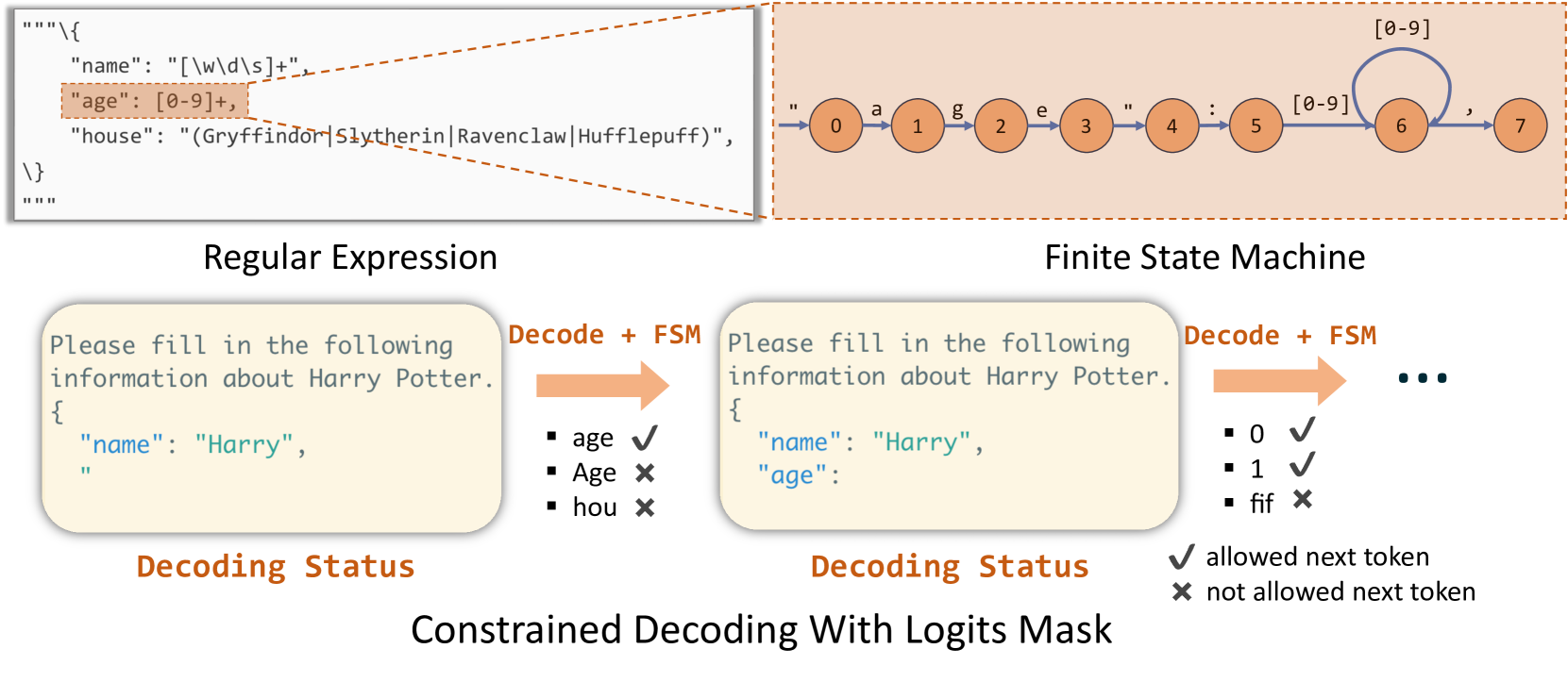
### Visual Description
# Technical Document: Constrained Decoding With Logits Mask
This document describes a technical diagram illustrating the process of using Regular Expressions and Finite State Machines (FSM) to constrain the output of a Large Language Model (LLM) during decoding.
## 1. Top Section: Pattern Definition
### Regular Expression (Left)
The diagram shows a JSON-like schema defined using regular expressions:
```json
"""{
"name": "[\w\d\s]+",
"age": [0-9]+,
"house": "(Gryffindor|Slytherin|Ravenclaw|Hufflepuff)",
}
"""
```
The line `"age": [0-9]+,` is highlighted in orange, indicating it is the focus of the subsequent FSM diagram.
### Finite State Machine (Right)
A state transition diagram represents the highlighted regular expression for the "age" field.
* **States:** 8 circular nodes labeled **0** through **7**.
* **Transitions:**
* **0 → 1:** labeled with `"` (double quote)
* **1 → 2:** labeled with `a`
* **2 → 3:** labeled with `g`
* **3 → 4:** labeled with `e`
* **4 → 5:** labeled with `"` (double quote)
* **5 → 6:** labeled with `:` (colon)
* **6 → 6:** self-loop labeled with `[0-9]` (indicates one or more digits)
* **6 → 7:** labeled with `,` (comma)
---
## 2. Bottom Section: Constrained Decoding Flow
The bottom half illustrates the step-by-step "Decoding Status" as the model generates text, using the FSM to mask invalid tokens.
### Step 1: Initial Decoding Status
* **Current Text:**
```text
Please fill in the following information about Harry Potter.
{
"name": "Harry",
"
```
* **Action (Decode + FSM):** An orange arrow points to a validation list.
* **Token Validation:**
* `age` ✔ (Allowed: matches the next expected sequence in the schema)
* `Age` ✘ (Not allowed: case-sensitive mismatch)
* `hou` ✘ (Not allowed: "house" is not the next expected key)
### Step 2: Updated Decoding Status
* **Current Text:**
```text
Please fill in the following information about Harry Potter.
{
"name": "Harry",
"age":
```
* **Action (Decode + FSM):** An orange arrow points to a validation list for the value of the "age" field.
* **Token Validation:**
* `0` ✔ (Allowed: matches `[0-9]`)
* `1` ✔ (Allowed: matches `[0-9]`)
* `fif` ✘ (Not allowed: alphabetical characters are not permitted in the numeric age field)
### Legend
* **✔**: allowed next token
* **✘**: not allowed next token
---
## 3. Summary of Logic
The diagram demonstrates **Constrained Decoding With Logits Masking**. By converting a schema (Regular Expression) into a Finite State Machine, the system can determine exactly which tokens are valid at any given point in the generation. Tokens that do not match the FSM transitions are masked (assigned a probability of zero), ensuring the LLM output strictly adheres to the predefined JSON format.
</details>
Figure 10: Example of how regex is converted into FSM and how FSM guides the decoding process.
The challenge of constrained decoding arises from the fact that constraints are often expressed in natural language formats, i.e., regex is depicted by characters/strings, while LLMs are designed to interpret and process these as tokens. This creates a complex scenario since the mapping between strings and tokens is intricate and lacks a one-to-one correspondence [22].
This section is derived from an earlier blog post https://lmsys.org/blog/2024-02-05-compressed-fsm/. Readers are also encouraged to read the blog post for additional background and easier understanding.
B.1 Implementation Details of Compressed Finite State Machine
To simplify the construction of Compressed FSM, we build the original FSM on characters/strings instead of on tokens. We formally define the concepts of singular transition edge and compressed edge as follows:
- Singular transition edge: A edge is a singular transition edge if 1) its source node has only one successor node, and 2) there is only one acceptable character/string on it.
- Compressed edge: An edge compressed by several consecutively adjacent edges $(e_{0},e_{1},...,e_{k})$ if and only if $e_{1},...,e_{k}$ are singular transition edges. The text of the compressed edge is the concatenation of the texts of $e_{0},e_{1},...,e_{k}$ .
Starting from an FSM based on characters, we recursively merge singular transition edges into their preceding ones until further compression is unfeasible, resulting in a Compressed FSM. This approach speeds up the decoding process, as demonstrated by SGLang’s runtime efficiency with the Compressed FSM, shown in Fig. 11.
<details>
<summary>x11.png Details</summary>
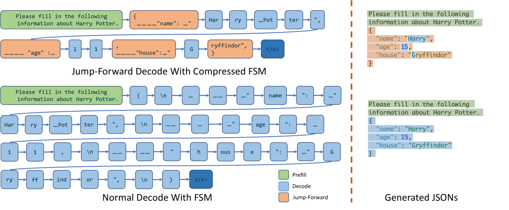
### Visual Description
# Technical Diagram Analysis: Jump-Forward vs. Normal Decode with FSM
This technical illustration compares two methods of Large Language Model (LLM) decoding for structured data (JSON): **Jump-Forward Decode With Compressed FSM** and **Normal Decode With FSM**.
## 1. Legend and Color Coding
The diagram uses a color-coded legend located in the bottom-right quadrant of the main chart area:
* **Green (Prefill):** Represents the initial prompt processing.
* **Light Blue (Decode):** Represents standard token-by-token generation.
* **Orange (Jump-Forward):** Represents compressed or skipped segments where multiple characters/tokens are handled in a single step.
* **Dark Blue (End of Sequence):** Represents the `</s>` token.
---
## 2. Component Analysis
### A. Top Section: Jump-Forward Decode With Compressed FSM
This flow demonstrates a more efficient decoding process by "jumping forward" through known structural elements of the JSON schema.
**Sequence Flow:**
1. **Prefill (Green):** `Please fill in the following information about Harry Potter.`
2. **Jump-Forward (Orange):** `{____"name": _"` (Structural boilerplate)
3. **Decode (Blue):** `Har` -> `ry` -> `_Pot` -> `ter` -> `",` (Variable content)
4. **Jump-Forward (Orange):** `____"age" :_` (Structural boilerplate)
5. **Decode (Blue):** `1` -> `1` (Variable content)
6. **Jump-Forward (Orange):** `,____"house":_"` (Structural boilerplate)
7. **Decode (Blue):** `G` (Variable content)
8. **Jump-Forward (Orange):** `ryffindor", }` (Structural boilerplate/completion)
9. **End (Dark Blue):** `</s>`
### B. Bottom Section: Normal Decode With FSM
This flow demonstrates standard token-by-token generation where every character and structural element is processed as an individual step.
**Sequence Flow:**
1. **Prefill (Green):** `Please fill in the following information about Harry Potter.`
2. **Decode (Blue):** A long sequence of individual tokens:
* Row 1: `{` -> `\n` -> `_` -> `__` -> `_"` -> `name` -> `":` -> `_"`
* Row 2: `Har` -> `ry` -> `_Pot` -> `ter` -> `",` -> `\n` -> `__` -> `_` -> `_"` -> `age` -> `":` -> `_`
* Row 3: `1` -> `1` -> `,` -> `\n` -> `__` -> `__` -> `"` -> `h` -> `ous` -> `e` -> `":` -> `_"` -> `G`
* Row 4: `ry` -> `ff` -> `ind` -> `or` -> `",` -> `\n` -> `}`
3. **End (Dark Blue):** `</s>`
---
## 3. Right Section: Generated JSONs
This section shows the final output resulting from the processes, highlighting which parts were generated via which method.
### Top JSON (Result of Jump-Forward)
* **Green Highlight:** `Please fill in the following information about Harry Potter.`
* **Orange Highlight (Structural):** `{`, `"name": "`, `",`, `"age": `, `,`, `"house": "`, `"` , `}`
* **Blue Highlight (Content):** `Harry`, `11`, `Gryffindor`
### Bottom JSON (Result of Normal Decode)
* **Green Highlight:** `Please fill in the following information about Harry Potter.`
* **Blue Highlight (Entirety):** The entire JSON structure and content are highlighted in blue, indicating every character was processed through standard decoding.
```json
{
"name": "Harry",
"age": 11,
"house": "Gryffindor"
}
```
---
## 4. Key Trends and Observations
* **Efficiency:** The "Jump-Forward" method significantly reduces the number of decoding steps (nodes in the graph) by grouping static structural elements (like JSON keys and punctuation) into single "Jump-Forward" blocks.
* **Step Count:** The Normal Decode requires approximately 40+ individual steps to generate the JSON, whereas the Jump-Forward method achieves the same result in roughly 13 steps.
* **Data Consistency:** Both methods produce the identical final JSON object containing the name "Harry Potter" (shortened to "Harry" in the final JSON view), age "11", and house "Gryffindor".
</details>
Figure 11: Comparison of decoding using Compressed FSM versus normal FSM: The left subfigure depicts the decoding process per forward pass, while the right subfigure explains the origins of various result components.
B.2 Handling Tokenization Artifacts with Retokenization
When a new token is generated, we get the token’s string and search all the outgoing edges of the current state find the one that starts with the just decoded string, and then move forward. However, when the transition edge is a well-compressed one and contains a very long string, we may anticipate the next rounds’ decoded strings as well. This is where the acceleration happens and we call this process Jump Forward. However, we still need to convert the string into tokens for the next decoding phases and it is not straightforward due to the LLM’s specific pretraining and tokenization method; direct partitioning might alter the intended meaning [50]. For example, the compressed text in Fig. 2 ’s regex is {"summary": ", which can only be tokenized as {", summary, ": and _" according to the tokenizer instead of partition them randomly such as {", summa, ry, and ":_". To address this issue, we use the original tokenizer to retokenize all the previous text as well as the text of the compressed edge, ensuring alignment with the original input format of LLMs. And it only brings minor retokenization overhead.
B.3 Future Extension: Addressing Distorted Probability
The challenge caused by the gap between strings and tokens also brings the problem of skewed probability distribution [50]. For example, in Fig. 2, the regex "[ABCD][+-]?" suggests grades from A+ to D-, but if replaced with broader terms like Excellent|Above Average|Fair|Below Average, the runtime may inaccurately map an A to Above Average due to the term Above Average is on a compressed transition, misrepresenting the grade hierarchy. This occurs because the LLM doesn’t recognize the specific range of choices, leading to inappropriate token sequences. Computing accurate probabilities for each choice requires summing the probabilities of all token sequences that result in each choice, which complicates decoding and adds overhead. One workaround is to include the choices or the regex directly in the prefill prompt, guiding the LLM to be aware of its choices and output the decision in proper token sequences. However, this approach doesn’t solve the underlying issue of distorted probabilities, highlighting the need for further research to improve the compressed FSM’s accuracy.
Appendix C Additional Experimental Setups and Results
Additional experimental setups. Fig. 5 and Fig. 6 are obtained by running Llama-7B on a single A10G (24GB) GPU. Fig. 7 are obtained by running Mixtral-8x7B on 8 A10G (24GB) GPUs with tensor parallelism. Fig. 8 (c) is obtained by running Llama-7B on a single A10G (24GB) GPU. Fig. 12 are obtained by running Llama-70B on 4 A100G (80GB) GPUs with tensor parallelism. Table 2 are obtained by running LLaVA-v1.5-7B on a single A10G (24GB) GPU and running LLaVA-Next-34B on a single A100G (80GB) GPU. Each bar in the benchmark figures takes several minutes to an hour to run.
Additional experimental results. Fig. 13 shows the achieved and optimal cache hit rates on the benchmarks listed in Fig. 5. Fig. 12 shows the throughput on Llama-2-70B with tensor parallelism.
<details>
<summary>x12.png Details</summary>
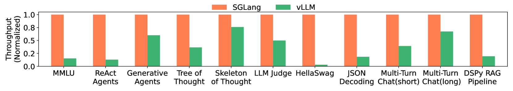
### Visual Description
# Technical Data Extraction: Throughput Comparison Chart
## 1. Component Isolation
* **Header (Legend):** Located at the top center. Contains two colored squares with labels:
* **Orange Square:** SGLang
* **Green Square:** vLLM
* **Main Chart Area:** A grouped bar chart comparing normalized throughput across 11 different benchmarks/tasks.
* **Y-Axis (Left):** Labeled "Throughput (Normalized)". Scale ranges from 0.0 to 1.0 with increments of 0.2.
* **X-Axis (Bottom):** Contains 11 categorical labels representing different LLM tasks/benchmarks.
---
## 2. Data Table Reconstruction
The following table represents the normalized throughput values extracted from the bar heights. Values for SGLang are consistently at the baseline of 1.0, while vLLM values are estimated based on the y-axis scale.
| Benchmark / Task | SGLang (Orange) | vLLM (Green) |
| :--- | :---: | :---: |
| **MMLU** | 1.0 | ~0.15 |
| **ReAct Agents** | 1.0 | ~0.12 |
| **Generative Agents** | 1.0 | ~0.60 |
| **Tree of Thought** | 1.0 | ~0.35 |
| **Skeleton of Thought** | 1.0 | ~0.75 |
| **LLM Judge** | 1.0 | ~0.50 |
| **HellaSwag** | 1.0 | ~0.03 |
| **JSON Decoding** | 1.0 | ~0.18 |
| **Multi-Turn Chat (short)** | 1.0 | ~0.40 |
| **Multi-Turn Chat (long)** | 1.0 | ~0.68 |
| **DSPy RAG Pipeline** | 1.0 | ~0.20 |
---
## 3. Trend Verification and Analysis
### SGLang (Orange Bars)
* **Visual Trend:** A perfectly flat horizontal line across all categories at the 1.0 mark.
* **Interpretation:** SGLang serves as the performance baseline (1.0) for this comparison.
### vLLM (Green Bars)
* **Visual Trend:** Highly variable performance relative to the baseline. The bars are significantly shorter than the orange bars in every single category.
* **Performance Peaks:** vLLM performs best (closest to SGLang) in "Skeleton of Thought" (~0.75) and "Multi-Turn Chat (long)" (~0.68).
* **Performance Valleys:** vLLM shows the lowest relative throughput in "HellaSwag" (near zero), "ReAct Agents," and "MMLU."
---
## 4. Summary of Findings
The chart demonstrates that **SGLang** consistently achieves higher throughput than **vLLM** across all 11 tested benchmarks. In several cases (HellaSwag, ReAct Agents, MMLU, JSON Decoding, and DSPy RAG Pipeline), SGLang's throughput is multiple times higher than that of vLLM. The gap is narrowest in "Skeleton of Thought" and "Multi-Turn Chat (long)," though SGLang still maintains a clear lead.
</details>
Figure 12: Normalized throughput on Llama-2-70B models with tensor parallelism. Higher is better.
<details>
<summary>x13.png Details</summary>
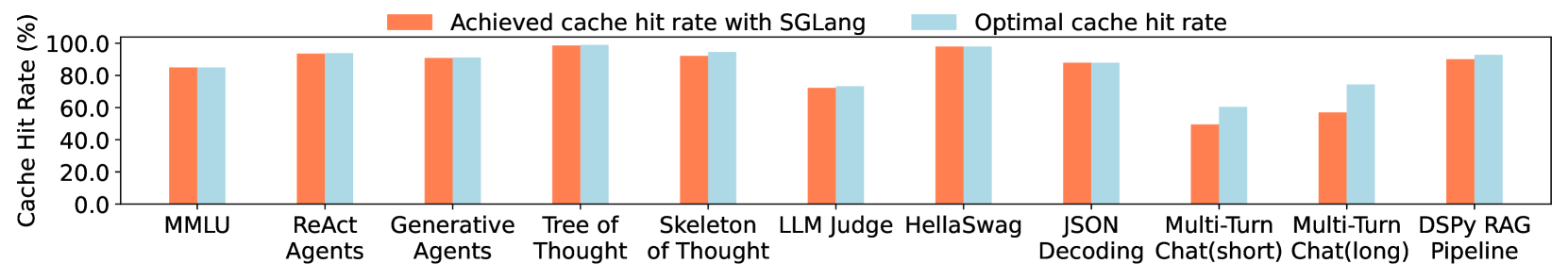
### Visual Description
# Technical Data Extraction: Cache Hit Rate Comparison
## 1. Image Overview
This image is a grouped bar chart comparing the performance of **SGLang** against an **Optimal** baseline across eleven different Large Language Model (LLM) benchmarks and tasks. The metric measured is the **Cache Hit Rate (%)**.
## 2. Chart Metadata
* **Y-Axis Title:** Cache Hit Rate (%)
* **Y-Axis Scale:** 0.0 to 100.0 (increments of 20.0)
* **X-Axis Categories:** 11 distinct LLM tasks/benchmarks.
* **Legend (Top Center):**
* **Orange Bar:** Achieved cache hit rate with SGLang
* **Light Blue Bar:** Optimal cache hit rate
## 3. Data Table Extraction
The following table reconstructs the visual data points. Values are estimated based on the Y-axis markers.
| Task / Benchmark | Achieved (SGLang - Orange) | Optimal (Light Blue) | Gap Analysis |
| :--- | :---: | :---: | :--- |
| **MMLU** | ~85% | ~85% | Identical |
| **ReAct Agents** | ~94% | ~94% | Identical |
| **Generative Agents** | ~91% | ~91% | Identical |
| **Tree of Thought** | ~98% | ~99% | Negligible gap |
| **Skeleton of Thought** | ~92% | ~95% | Small gap |
| **LLM Judge** | ~72% | ~73% | Negligible gap |
| **HellaSwag** | ~98% | ~98% | Identical |
| **JSON Decoding** | ~88% | ~88% | Identical |
| **Multi-Turn Chat (short)** | ~50% | ~60% | Moderate gap |
| **Multi-Turn Chat (long)** | ~57% | ~74% | Significant gap |
| **DSPy RAG Pipeline** | ~90% | ~93% | Small gap |
## 4. Component Analysis and Trends
### Header/Legend Region
The legend is positioned at the top center. It clearly distinguishes between the practical implementation (SGLang) and the theoretical maximum (Optimal).
### Main Chart Region (Trends)
* **High Performance Consistency:** In 7 out of 11 tasks (MMLU, ReAct Agents, Generative Agents, Tree of Thought, HellaSwag, JSON Decoding, and DSPy RAG), SGLang achieves a cache hit rate that is either identical or nearly identical to the optimal rate, typically exceeding 85%.
* **Complexity Sensitivity:** The performance gap between SGLang and the Optimal rate widens significantly in "Multi-Turn Chat" scenarios.
* In **Multi-Turn Chat (short)**, there is a visible ~10% discrepancy.
* In **Multi-Turn Chat (long)**, the discrepancy is at its largest (approx. 17%), indicating that longer conversational contexts are more challenging for the current SGLang caching implementation to optimize fully.
* **Lowest Overall Hit Rate:** The "Multi-Turn Chat (short)" task shows the lowest achieved hit rate for SGLang at approximately 50%.
* **Highest Overall Hit Rate:** "Tree of Thought" and "HellaSwag" show the highest efficiency, nearing 100% cache hit rates.
### Footer/X-Axis Region
The labels are clearly legible and categorized by task type, ranging from standard benchmarks (MMLU, HellaSwag) to specific architectural patterns (ReAct, Tree of Thought, RAG).
</details>
Figure 13: Achieved cache hit rate and optimal cache hit rate on various benchmarks.
<details>
<summary>x14.png Details</summary>
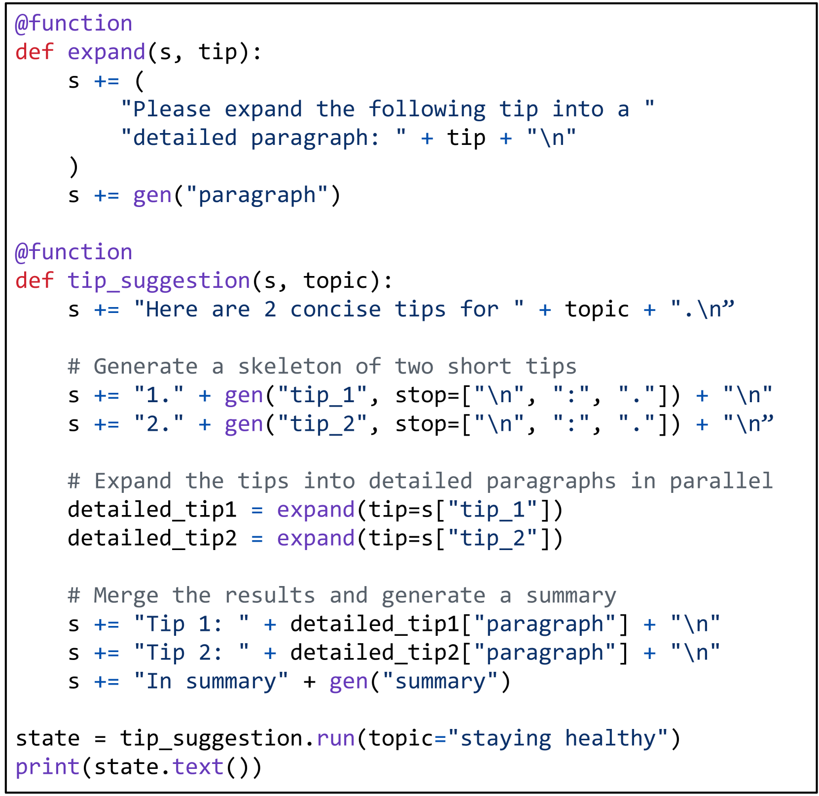
### Visual Description
# Technical Document Extraction: Python Code Snippet
## 1. Overview
The image contains a Python code snippet utilizing a domain-specific language or framework (likely for LLM prompting/generation) characterized by the `@function` decorator and a `gen()` function. The code defines a workflow to generate concise tips on a topic and then expand those tips into detailed paragraphs.
## 2. Code Transcription
```python
@function
def expand(s, tip):
s += (
"Please expand the following tip into a "
"detailed paragraph: " + tip + "\n"
)
s += gen("paragraph")
@function
def tip_suggestion(s, topic):
s += "Here are 2 concise tips for " + topic + ".\n"
# Generate a skeleton of two short tips
s += "1." + gen("tip_1", stop=["\n", ":", "."]) + "\n"
s += "2." + gen("tip_2", stop=["\n", ":", "."]) + "\n"
# Expand the tips into detailed paragraphs in parallel
detailed_tip1 = expand(tip=s["tip_1"])
detailed_tip2 = expand(tip=s["tip_2"])
# Merge the results and generate a summary
s += "Tip 1: " + detailed_tip1["paragraph"] + "\n"
s += "Tip 2: " + detailed_tip2["paragraph"] + "\n"
s += "In summary" + gen("summary")
state = tip_suggestion.run(topic="staying healthy")
print(state.text())
```
## 3. Component Analysis and Logic Flow
### Functions
* **`expand(s, tip)`**:
* **Input**: Takes a state object `s` and a string `tip`.
* **Logic**: Appends a prompt instruction to the state and calls `gen("paragraph")` to generate a long-form expansion of the provided tip.
* **`tip_suggestion(s, topic)`**:
* **Input**: Takes a state object `s` and a string `topic`.
* **Step 1 (Skeleton Generation)**: Appends an introductory sentence. It then generates two short strings (`tip_1` and `tip_2`) using specific stop sequences (`\n`, `:`, `.`) to ensure brevity.
* **Step 2 (Parallel Expansion)**: Calls the `expand` function twice. Note that the syntax `expand(tip=s["tip_1"])` suggests these are treated as sub-tasks or parallelizable units.
* **Step 3 (Merging/Summary)**: Concatenates the "paragraph" results from the expansion tasks back into the main state `s` and generates a final "summary" section.
### Execution
* **Initialization**: The variable `state` is assigned the result of `tip_suggestion.run(topic="staying healthy")`.
* **Output**: The final text content of the processed state is printed to the console via `print(state.text())`.
## 4. Syntax and Formatting Details
* **Decorators**: Both functions are preceded by `@function`.
* **String Concatenation**: Uses the `+=` operator and `+` for building prompts.
* **Comments**:
* `# Generate a skeleton of two short tips`
* `# Expand the tips into detailed paragraphs in parallel`
* `# Merge the results and generate a summary`
* **Color Coding (Syntax Highlighting)**:
* **Purple**: Decorators (`@function`) and built-in functions/methods (`gen`, `print`, `.run`, `.text`).
* **Red/Brown**: Keywords (`def`).
* **Blue**: Function names (`expand`, `tip_suggestion`) and variable names (`s`, `tip`, `topic`, `detailed_tip1`, `detailed_tip2`, `state`).
* **Blue (Strings)**: Text enclosed in quotes.
* **Grey**: Comments.
</details>
(a) The SGLang program for parallel tip suggestion with skeleton-of-thought prompting.
<details>
<summary>x15.png Details</summary>
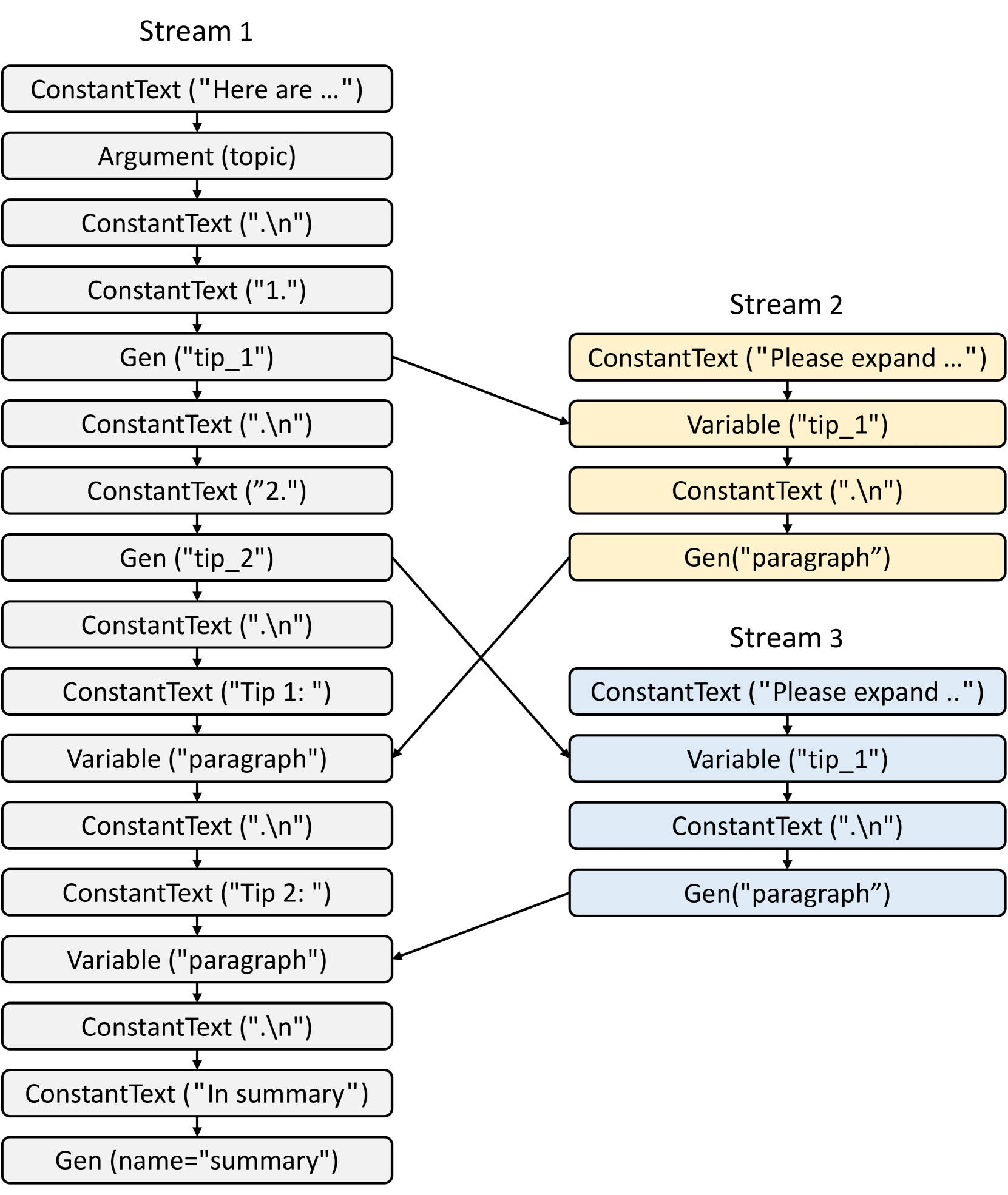
### Visual Description
# Technical Diagram Analysis: Multi-Stream Text Generation Flow
This diagram illustrates a parallelized text generation process involving three distinct streams (Stream 1, Stream 2, and Stream 3). It details the sequential logic of constant text insertion, variable handling, and generation calls, as well as the cross-stream dependencies.
## 1. Component Overview
The diagram consists of three vertical columns representing processing streams. Each stream contains a series of rounded rectangular nodes connected by downward arrows indicating sequential flow. Diagonal arrows indicate data dependencies between streams.
* **Stream 1 (Grey):** The primary control flow and final output assembly.
* **Stream 2 (Yellow):** A secondary generation stream for expanding specific content.
* **Stream 3 (Blue):** A tertiary generation stream for expanding specific content.
---
## 2. Detailed Stream Breakdown
### Stream 1 (Primary)
This stream follows a linear sequence with 17 distinct steps:
1. **ConstantText ("Here are ...")**
2. **Argument (topic)**
3. **ConstantText (".\n")**
4. **ConstantText ("1.")**
5. **Gen ("tip_1")** -> *Output feeds into Stream 2 and Stream 3.*
6. **ConstantText (".\n")**
7. **ConstantText ("2.")**
8. **Gen ("tip_2")** -> *Output feeds into Stream 3.*
9. **ConstantText (".\n")**
10. **ConstantText ("Tip 1: ")**
11. **Variable ("paragraph")** <- *Input received from Stream 2.*
12. **ConstantText (".\n")**
13. **ConstantText ("Tip 2: ")**
14. **Variable ("paragraph")** <- *Input received from Stream 3.*
15. **ConstantText (".\n")**
16. **ConstantText ("In summary")**
17. **Gen (name="summary")**
### Stream 2 (Secondary - Yellow)
Triggered by data from Stream 1, containing 4 steps:
1. **ConstantText ("Please expand ...")**
2. **Variable ("tip_1")** <- *Data sourced from Stream 1, Step 5.*
3. **ConstantText (".\n")**
4. **Gen ("paragraph")** -> *Output feeds back to Stream 1, Step 11.*
### Stream 3 (Tertiary - Blue)
Triggered by data from Stream 1, containing 4 steps:
1. **ConstantText ("Please expand ..")**
2. **Variable ("tip_1")** <- *Data sourced from Stream 1, Step 5.*
3. **ConstantText (".\n")**
4. **Gen ("paragraph")** -> *Output feeds back to Stream 1, Step 14.*
---
## 3. Cross-Stream Data Dependencies (Spatial Grounding)
The diagram uses diagonal arrows to show how generated outputs from one stream become variables in another:
| Source Node | Target Node | Direction |
| :--- | :--- | :--- |
| **Stream 1:** Gen ("tip_1") | **Stream 2:** Variable ("tip_1") | Down-Right |
| **Stream 1:** Gen ("tip_1") | **Stream 3:** Variable ("tip_1") | Down-Right |
| **Stream 1:** Gen ("tip_2") | **Stream 3:** Variable ("tip_1")* | Down-Right |
| **Stream 2:** Gen ("paragraph") | **Stream 1:** Variable ("paragraph") (Step 11) | Down-Left |
| **Stream 3:** Gen ("paragraph") | **Stream 1:** Variable ("paragraph") (Step 14) | Down-Left |
*\*Note: There is a visual overlap where the arrow from Stream 1's Gen ("tip_2") points toward the Variable node in Stream 3, which is labeled "tip_1". This suggests a potential mapping or reuse of the variable slot.*
---
## 4. Summary of Logic
The system initiates by setting a topic and generating two "tips" in Stream 1. These tips are then sent to parallel streams (2 and 3) where they are expanded into full paragraphs. Once the parallel streams complete their generation, the resulting "paragraphs" are pulled back into Stream 1 to be formatted into a final document that concludes with a generated summary.
</details>
(b) A computational graph for the program in 14(a). The three streams correspond to three function calls.
Figure 14: An SGLang program and its corresponding dataflow graph.
Appendix D Compiler Mode
Besides the interpreter mode used in the main body of the paper, another way to run SGLang programs is to compile them as computational graphs and execute them with a graph executor. This opens up opportunities for more compilation optimizations, as we can rewrite the graph and perform more static planning.
D.1 Design and Implementation
We designed an intermediate representation (IR) for SGLang, which represents SGLang program structures and operations as a computational graph. This graph includes nodes for primitive operators and edges for dependencies. See 14(b) for the graph corresponding to the program in 14(a). In the program, each call to a decorated function or fork creates a new prompt state or a stream.
There are several types of nodes. Each operand of the operators += and + in a SGLang program is represented by an IR node. These include ConstantText, Argument, Gen, Select, Variable, Fork, GetForkItem, and Join. There are two types of dependencies: intra-stream dependency, where operations submitted into a stream using += must be executed after all preceding operations in that stream, and inter-stream dependency, which occurs when one stream needs to fetch variable values from another stream, necessitating synchronization. Operations like fork manipulate multiple streams and thus introduce inter-stream dependencies.
To generate the graph, we use tracing to run the program with abstract arguments and construct the graph dynamically. This method is limited to programs without data-dependent control flow, a limitation we plan to address in future work. Once constructed, the graph can be executed through a graph executor, eliminating the need to reinterpret the original Python program. This results in benefits like graph rewriting optimizations, reduced runtime overhead, and program serialization. For execution, stream executors are launched for each data stream, dispatching IR nodes to the streams in topological order.
D.2 A Case Study of Compiler Optimization: Code Movement for Improving Prefix Sharing
We explore a compilation optimization for SGLang IR: code movement for improving prefix sharing. We anticipate that more classical compiler techniques can also be applied, such as auto-tuning and instruction selection.
This optimization aims to improve prefix sharing by reordering nodes in the graph to increase the length of the constant prefix. It does not strictly preserve the original computation, classifying it as an aggressive optimization. For instance, changing the prompt from “Here is a question + {question}. Please act as a math expert and solve the given question.” to “Please act as a math expert and solve the given question. Here is a question + {question}.” results in a longer shareable prefix. This optimization is interesting because traditional program analysis cannot achieve it due to the presence of natural language instructions in SGLang. Instead, we prompt GPT-4 to reorder graph nodes. We write a prompt with several examples to teach GPT-4 the concepts of SGLang IR, and we find that GPT-4 can successfully apply this optimization for some simple SGLang programs.
We evaluate the effectiveness of this optimization. We collect 20 prompt templates from the internet and implement them in SGLang. We utilize 5 of these templates as few-shot training examples and the remaining 15 as test cases. Our evaluation shows that, for 12 out of the 15 templates, GPT-4 successfully reorders the graph nodes without altering the semantics, as confirmed by manual inspection of the modified prompts. On average, this optimization results in a 60-token increase in the shareable prefix length, showcasing GPT-4’s effectiveness. Failures in creating optimized prompt order come from an incorrect understanding of the semantic meaning behind the graph nodes. It is too aggressive and puts all constants upfront even when such ordering changes the original semantics. This case study aims to explore the use of GPT-4 for compiler optimizations. More work is needed to make these kinds of optimizations reliable in the future.