2312.07547

# Active Inference and Intentional Behaviour **Authors**: Karl J. Friston, Tommaso Salvatori, Takuya Isomura, Alexander Tschantz, Alex Kiefer, Tim Verbelen, Magnus Koudahl, Aswin Paul, Thomas Parr, Adeel Razi, Brett Kagan, Christopher L. Buckley, Maxwell J. D. Ramstead > Wellcome Trust Centre for Neuroimaging, Institute of Neurology, University College London, UK. VERSES AI Research Lab, Los Angeles, California, 90016, USA > VERSES AI Research Lab, Los Angeles, California, 90016, USA > Brain Intelligence Theory Unit, RIKEN Center for Brain Science, Wako, Saitama, Japan > VERSES AI Research Lab, Los Angeles, California, 90016, USA Nuffield Department of Clinical Neurosciences, University of Oxford, UK > VERSES AI Research Lab, Los Angeles, California, 90016, USA Turner Institute for Brain and Mental Health, School of Psychological Sciences, Monash University, Clayton, Australia IITB-Monash Research Academy, Mumbai-76, India > Nuffield Department of Clinical Neurosciences, University of Oxford, UK > Turner Institute for Brain and Mental Health, School of Psychological Sciences, Monash University, Clayton, Australia Monash Biomedical Imaging, Monash University, Clayton, Australia CIFAR Azrieli Global Scholars Program, Toronto, Canada > Cortical Labs, Melbourne, Australia ## Abstract Recent advances in theoretical biology suggest that basal cognition and sentient behaviour are emergent properties of in vitro cell cultures and neuronal networks, respectively. Such neuronal networks spontaneously learn structured behaviours in the absence of reward or reinforcement. In this paper, we characterise this kind of self-organisation through the lens of the free energy principle, i.e., as self-evidencing. We do this by first discussing the definitions of reactive and sentient behaviour in the setting of active inference, which describes the behaviour of agents that model the consequences of their actions. We then introduce a formal account of intentional behaviour, that describes agents as driven by a preferred endpoint or goal in latent state-spaces. We then investigate these forms of (reactive, sentient, and intentional) behaviour using simulations. First, we simulate the aforementioned in vitro experiments, in which neuronal cultures spontaneously learn to play Pong, by implementing nested, free energy minimising processes. The simulations are then used to deconstruct the ensuing predictive behaviour—leading to the distinction between merely reactive, sentient, and intentional behaviour, with the latter formalised in terms of inductive planning. This distinction is further studied using simple machine learning benchmarks (navigation in a grid world and the Tower of Hanoi problem), that show how quickly and efficiently adaptive behaviour emerges under an inductive form of active inference. Keywords: active inference; active learning; backwards induction;planning as inference; free energy principle. ## 1 Introduction In 2022, a paper was published that claimed to demonstrate sentient behaviour in a neuronal culture grown in a dish (an in vitro neuronal network) [1]. The behaviour in question was the spontaneous emergence of controlled movements of a paddle to hit a ball—and thereby play Pong. This study has several sources of inspiration that speak to the notion of basal cognition; see, e.g., [2, 3, 4] (and related work, e.g. [5]). In particular, the hypothesis that adaptive and predictive behaviour would emerge spontaneously was based on earlier work showing that in vitro neuronal cultures could be described as minimising variational free energy [6] and thereby evince active inference and learning. This application of the free energy principle (FEP) to neuronal cultures was subsequently validated empirically [7]: in the sense that changes in neuronal activity and synaptic efficacy—that underwrite learning—could be predicted quantitatively, as a variational free energy minimising process. So, are these findings remarkable, or were they predictable? In one sense, these results were entirely predictable. Indeed, they were predictable from the FEP, which states that any two networks—that are coupled in a certain sparse fashion—will come to manifest a generalised synchrony [8, 9]. More formally, the FEP states that if the probability density that underwrites the dynamics of coupled random dynamical systems contains a Markov blanket—which shields internal states from external states, given blanket (sensory and active) states—then internal states will look as if they track the statistics of external states—or more precisely, as if they encode the parameters of a variational density (or best guess about) external states beyond the blanket. Empirically, this synchronisation was observed when the neuronal cultures learned to play Pong. However, the FEP goes further and says that the internal and active states (together, autonomous states) of either network can be described as minimising a variational free energy functional. This functional is exactly the same used to optimise generative models in statistics and machine learning [10]. On this reading, one can interpret the autonomous states—of a network, particle or person—as minimising variational free energy or surprise (a.k.a., self-information) or, equivalently, maximising Bayesian model evidence (a.k.a., the marginal likelihood of sensory states). This leads to an implicit teleology, in the sense that one can describe self-organisation in terms of self-evidencing [11] that entails active inference and learning, planning, purpose, intentions and, perhaps, sentience. The underlying free energy minimising processes—and their teleological interpretation—are the focus of this paper. The results reported in [1] were considered by some to be unremarkable for a different reason: learning to play (Atari) games like Pong was something that had been accomplished with machine learning systems years earlier using neural networks and (deep) reinforcement learning [12, 13]. So, what is remarkable about a neuronal network reproducing the same kind of behaviour? It is remarkable because one cannot use the reinforcement learning (RL) paradigm to explain the emergence of self-evidencing behaviour seen in vitro. This follows from the fact that one cannot reward a neuronal network—because no one knows what any given in vitro neuronal network finds rewarding. However, the FEP theorist knows exactly what a self-evidencing network finds aversive; namely, surprise and unpredictability. This was a rationale for delivering unpredictable noise to the sensory electrodes of the cell culture (or restarting the game in an unpredictable way), whenever the neuronal network failed to hit the ball [1]. Some found the results reported in [1] remarkable, but not in a good way: they disagreed with the claim that the behaviour could be described as ‘sentient’ [14]. Here, we hope to make sense of the notion of sentient behaviour in terms of Bayesian belief updating; where ‘sentient behaviour’ denotes the capacity to generate appropriate responses to sensory perturbations (as opposed to merely reactive behaviour). We pursue the narrative established by the cell culture experiments above to illustrate why Pong-playing behaviour was considered sentient, as opposed to reactive. In brief, we consider a bright line between actions based upon the predictions of a generative model that does, and does not, entail the consequences of action. Specifically, this paper differentiates between three kinds of behaviour: reactive, sentient, and intentional. The first two have formulations that have been extensively studied in the literature, under the frameworks of model-free reinforcement learning (RL) and active inference, respectively. In model-free RL, the system selects actions using either a lookup table (Q-learning), or a neural network (deep Q-learning). In standard active inference, the action selection depends on the expected free energy of policies (Equation 2), where the expectation is over observations in the future that become random variables. This means that preferred outcomes—that subtend expected cost and risk—are prior beliefs that constrain the implicit planning as inference [15, 16, 17]. Things that evince this kind of behaviour can hence be described as planning their actions, based upon a generative model of the consequences of those actions [15, 16, 18]. It was this sense in which the behaviour of the cell cultures was considered sentient. This form of sentient behaviour —described in terms of Bayesian mechanics [19, 20, 21] —can be augmented with intended endpoints or goals. This leads to a novel kind of sentient behaviour that not only predicts the consequences of its actions, but is also able to select them to reach a goal state that may be many steps in the future. This kind of behaviour, that we call intentional behaviour, generally requires some form of backwards induction [22, 23] of the kind found in dynamic programming [24, 25, 26, 27]: this is, starting from the intended goal state, and working backwards, inductively, to the current state of affairs, in order to plan moves to that goal state. Backwards induction was applied to the partially observable setting and explored in the context of active inference in [27]. In that work, dynamic programming was shown to be more efficient than traditional planning methods in active inference. The focus of this work is to formally define a framework for intentional behaviour, where the agent minimises a constrained form of expected free energy—and to demonstrate this framework in silico. These constraints are defined on a subset of latent states that represent the intended goals of the agent, and propagated to the agent via a form of backward induction. As a result, states that do not allow the agent to make any ‘progress’ towards one of the intended goals are penalised, and so are actions that lead to such disfavoured states. This leads to a distinction between sentient and intentional behaviour, were intentional behaviour is equipped with inductive constraints. In this treatment, the word inductive is used in several senses. First, to distinguish inductive planning from the abductive kind of inference that usually figures in applications of Bayesian mechanics; i.e., to distinguish between mere inference to the best explanation (abductive inference) and genuinely goal-directed inference (inductive planning) [28, 29]. Second, it is used with a nod to backwards induction in dynamic programming, where one starts from an intended endpoint and works backwards in time to the present, to decide what to do next [24, 25, 30, 27]. Under this naturalisation of behaviours, a thermostat would not exhibit sentient behaviour, but insects might (i.e., thermostats exhibit merely reactive behaviour). Similarly, insects would not exhibit intentional behaviour, but mammals might (i.e., insects exhibit merely sentient behaviour). The numerical analyses presented below suggest that in vitro neuronal cultures may exhibit sentient behaviour, but not intentional behaviour. Crucially, we show that neither sentient nor intentional behaviour can be explained by reinforcement learning. In the experimental sections of this work, we study and compare the performance of active inference agents with and without intended goal states. For ease of reference, we will call active inference agents without goal states abductive agents, and agents with intended goals inductive agents. This paper comprises four sections. The first briefly rehearses active inference and learning—as a set of nested free energy minimising processes—applied to a generic generative model of exchange with some world or environment. This model is a partially observed Markov decision process that is conciliatory with canonical neural networks in machine learning and apt to describe the self-evidencing of in vitro neuronal networks [6, 7]. This section has a special focus on inductive planning and its relationship to expected free energy. The subsequent sections use numerical studies to make a series of key points. The second section reproduces the empirical behaviour of in vitro neuronal networks playing Pong. Crucially, this behaviour emerges purely in terms of free energy minimising processes, starting with a naïve neuronal network. This section illustrates the failure of a (simulated) abductive agent when the game is made more difficult. This failure is used to illustrate the role of inductive planning, which restores performance and underwrites a fluent engagement with the sensorium. The final two sections illustrate inductive planning using navigation in a maze and the Tower of Hanoi problem, respectively. These numerical studies illustrate how the simple application of inductive constraints to active inference allows tasks—that would be otherwise intractable in discrete state spaces—to be solved efficiently. This efficiency rests on the fact that distal goals can be reached by only planning a few steps in the future, thanks to constraints furnished by inductive planning. Effectively, inductive planning takes the pressure off deep tree searches by identifying ’blind alleys’ or ’dead ends’. ### 1.1 Glossary of definitions Before introducing the inductive planning algorithm, we frame our treatment by clarifying our use of some key terms. This framing is important, given that the goal of the present work is not simply to describe a useful heuristic for efficient inference (i.e., inductive planning), but to provide an account of how a new form of decision-making, characteristic of more complex forms of agency, may be combined with, and folded into, a generic Bayesian (active) inference scheme. 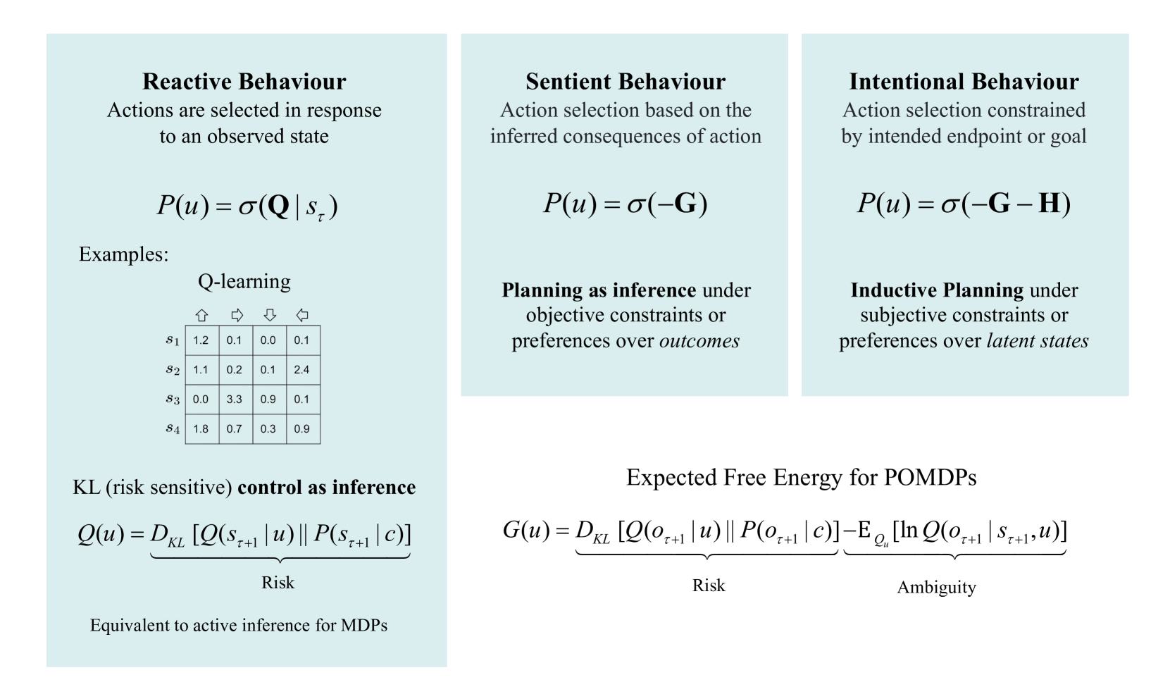Figure 1 describes increasingly complex forms of behaviour—from reactive (merely responding to stimuli), to sentient (planning based on the sensory consequences of actions), to intentional (planning in order to bring about intended states)—and corresponding forms of decision-making that may underwrite such behaviour. Reactive behaviour characterises simple sensorimotor reflex arcs and the mere realisation of set points or trajectories (e.g., simple cases of homeostasis and homeorhesis). This form of behaviour can be accounted for acting in a way that realises predicted sensations, with no anticipation of the future sensory consequences of action. Sentient behaviour characterises the paradigmatic case of active inference, in which the influence of perception on action is mediated by the results of planning, with a distribution over policies derived from a model endowed with counterfactual depth (i.e., beliefs about the future sensory consequences of action pursuant to a policy). In this case, we may characterise the form of inference over actions or policies as abductive —i.e., as an inference to the policy that best explains current and future observations under a generative model (see below). Intentional behaviour is driven not simply by the generic imperative to minimise sensory prediction error, present and future, but toward the attainment of a particular future endpoint or goal state. This form of behaviour can be subserved by backward induction or inductive planning, as defined below, which supplies a specific form of constraint on the Bayesian (abductive) inference characteristic of (mere) sentient behaviour. In particular, it implies not merely beliefs about sensory consequences of actions but rather beliefs about the inferred or latent causes of sensory input. Note that words like ‘sentient behaviour’ and ‘intentional behaviour’ are deliberately defined here such that they can be operationalized within the framework of generative modelling, in which terms like ‘state’, ‘belief’, and ‘confidence’ have precise, if narrow, interpretations in terms of belief structures of a mathematical sort [31]. Whether the phenomenology of (propositional or subjective) beliefs—or sentience—could yield to the same naturalisation remains to be seen: see [32, 33, 34] for treatments in this direction. Note further that a key distinction between sentient and intentional behaviour rests upon the consequences of behaviour in (observable) outcome and (unobservable) latent spaces, respectively. <details> <summary>x1.png Details</summary>  ### Visual Description \n ## Diagram: Comparison of Behavioural Frameworks in Active Inference ### Overview The image is a technical diagram comparing three paradigms of action selection within the framework of active inference and control as inference: **Reactive Behaviour**, **Sentient Behaviour**, and **Intentional Behaviour**. It presents their core definitions, mathematical formulations, and associated concepts. The diagram is structured into three vertical columns for the behaviour types, with a shared foundational section at the bottom. ### Components/Axes The diagram is organized into three primary vertical panels, each with a light blue background, and a white background section at the bottom. **1. Left Panel: Reactive Behaviour** * **Title:** "Reactive Behaviour" * **Description:** "Actions are selected in response to an observed state" * **Core Formula:** `P(u) = σ(Q | s_τ)` * **Examples Section:** Contains a sub-section titled "Q-learning" with a 4x4 data table. * **Additional Concept:** "KL (risk sensitive) **control as inference**" with the formula `Q(u) = D_KL [Q(s_{τ+1} | u) || P(s_{τ+1} | c)]`. The term `D_KL [...]` is underbraced and labeled "Risk". * **Footer Note:** "Equivalent to active inference for MDPs" **2. Middle Panel: Sentient Behaviour** * **Title:** "Sentient Behaviour" * **Description:** "Action selection based on the inferred consequences of action" * **Core Formula:** `P(u) = σ(-G)` * **Associated Concept:** "**Planning as inference** under objective constraints or preferences over *outcomes*" **3. Right Panel: Intentional Behaviour** * **Title:** "Intentional Behaviour" * **Description:** "Action selection constrained by intended endpoint or goal" * **Core Formula:** `P(u) = σ(-G - H)` * **Associated Concept:** "**Inductive Planning** under subjective constraints or preferences over *latent states*" **4. Bottom Section (Spanning Right Side):** * **Title:** "Expected Free Energy for POMDPs" * **Formula:** `G(u) = D_KL [Q(o_{τ+1} | u) || P(o_{τ+1} | c)] - E_{Q_u} [ln Q(o_{τ+1} | s_{τ+1}, u)]` * The first term `D_KL [...]` is underbraced and labeled "Risk". * The second term `- E_{Q_u} [...]` is underbraced and labeled "Ambiguity". ### Detailed Analysis **Q-Learning Table (Reactive Behaviour Example):** The table is a 4x4 matrix with rows labeled `s₁` to `s₄` (states) and columns indicated by directional arrow icons (↑, →, ↓, ←) representing actions. | State | ↑ | → | ↓ | ← | |-------|---|---|---|---| | s₁ | 1.2 | 0.1 | 0.0 | 0.1 | | s₂ | 1.1 | 0.2 | 0.1 | 2.4 | | s₃ | 0.0 | 3.3 | 0.9 | 0.1 | | s₄ | 1.8 | 0.7 | 0.3 | 0.9 | These values represent Q-values (expected rewards) for taking a specific action in a given state. **Mathematical Formulations:** * `σ` denotes a softmax function, converting values into a probability distribution over actions `u`. * `Q` in the Reactive formula represents the Q-value function. * `G` represents Expected Free Energy, decomposed into Risk and Ambiguity terms in the bottom formula. * `H` in the Intentional formula represents an additional term for subjective constraints or preferences over latent states. * `D_KL` denotes the Kullback-Leibler divergence. * `Q(s_{τ+1} | u)` and `P(s_{τ+1} | c)` represent posterior and prior distributions over next states, respectively. * `Q(o_{τ+1} | u)` and `P(o_{τ+1} | c)` represent posterior and prior distributions over next observations. * `E_{Q_u}[...]` denotes an expectation taken with respect to the distribution `Q_u`. ### Key Observations 1. **Progressive Complexity:** The three behaviour types show a clear progression in the complexity of the action selection rule: from `P(u) = σ(Q)` (Reactive), to `P(u) = σ(-G)` (Sentient), to `P(u) = σ(-G - H)` (Intentional). 2. **Unifying Framework:** All three paradigms are framed within "control as inference," where choosing an action is treated as probabilistic inference. 3. **Risk and Ambiguity:** The decomposition of Expected Free Energy (`G`) into "Risk" (divergence from preferred outcomes) and "Ambiguity" (information gain) is explicitly highlighted as foundational for planning in Partially Observable MDPs (POMDPs). 4. **Conceptual Mapping:** The diagram maps well-known algorithms to these paradigms: Q-learning is an example of Reactive Behaviour, "Planning as inference" aligns with Sentient Behaviour, and "Inductive Planning" aligns with Intentional Behaviour. ### Interpretation This diagram serves as a conceptual taxonomy for understanding different levels of cognitive sophistication in artificial agents, grounded in the mathematics of active inference. * **Reactive Behaviour** represents a stimulus-response mechanism. The agent acts based on cached values (`Q`) associated with the current state (`s_τ`), without explicitly simulating future consequences. The link to "KL control as inference" and "risk" suggests this can be viewed as minimizing a divergence from a desired state distribution, but in a myopic, state-conditioned way. It's equivalent to solving fully observable Markov Decision Processes (MDPs). * **Sentient Behaviour** introduces foresight. Action selection is guided by minimizing Expected Free Energy (`G`), which involves evaluating the *inferred consequences* of actions. This corresponds to "planning as inference" where the agent infers the most likely actions to achieve preferred *outcomes* (`o`). This is suitable for partially observable environments where the agent must reason about future observations. * **Intentional Behaviour** adds a layer of subjective preference or goal-directedness. The additional term `-H` modifies the planning objective to incorporate preferences over *latent states* (`s`), not just observable outcomes. This suggests a form of "inductive planning" where the agent has an internal model or intention (a preferred trajectory in state-space) that guides action selection beyond mere outcome preferences. **Underlying Message:** The diagram argues that complex, goal-directed (intentional) behaviour can be derived as an extension of simpler reactive and sentient mechanisms, all within a unified probabilistic framework. The progression from Q-values to Expected Free Energy to an augmented Free Energy (`G+H`) illustrates how increasingly abstract internal models (of states, outcomes, and latent preferences) enable more sophisticated planning. The explicit breakdown of `G` into Risk and Ambiguity underscores the dual objective in active inference: achieving goals (exploitation) and reducing uncertainty (exploration). </details> Figure 1: Glossary. In this figure, we provide illustrative definitions of the three kinds of behaviour considered in this work, In terms of examples, and mathematical differences. Examples of agents with reactive behaviours are (1) Model-free reinforcement learning schemes, such as Q-learning, where the agent makes use of a lookup table to select actions (more generally, a state-action policy). In this table, rows correspond to states, actions to columns, and every entry encodes the value of taking a specific action (in this case: go up, right, down, left) when in state $s_τ$ . There is no inference over policies, as for every state the agent automatically selects the action with the highest value; and (2) KL control (a.k.a., risk-sensitive control) methods, that automatically select actions that minimise a KL divergence between anticipated and preferred states (where there is no uncertainty about the current state). Sentient agents, on the other hand, plan by taking into account future outcomes and their uncertainty, as they act by minimising an expected free energy $G$ , that includes risk and ambiguity terms. More details on this can be found in Equation 5. Finally, inductive agents add constraints ( $H$ in the figure) in the action selection, by penalising actions that preclude an intended goal. For a formal derivation of $H$ , we refer to Section 3. ## 2 Active inference Here, we introduce the generative model used in the following sections, which can be seen as a generalisation of a partially observed Markov decision process (POMDP). The generalisation in question covers trajectories, narratives or syntax—which may or may not be controllable—by equipping a POMDP with random variables called paths. Paths effectively pick out transitions among latent states. These models are designed to be composed hierarchically, in a way that speaks to a separation of temporal scales in deep generative models. In other words, the number of transitions among latent states at any given level is greater than the number of transitions at the level above. This furnishes a unique specification of a hierarchy, in which the parents of any latent factor (associated with unique states and paths) contextualise the dynamics of their children. The variational inference scheme [35] used to invert these models inherits from their application to online decision-making tasks. This means that action selection rests primarily on current beliefs about latent states and structures, and expectations about future observations. In that sense, the beliefs are updated sequentially—and in an online fashion—with each new action-outcome pair. This calls for Bayesian filtering (i.e., forward message passing) during the active sampling of observations, followed by Bayesian smoothing (i.e., forward and backward message passing) to revise posterior beliefs about past states at the end of an epoch. The implicit Bayesian smoothing ensures that the beliefs about latent states at any moment in the past are informed by all available observations when updating model parameters (and latent states of parents in deep models). In neurobiology, this combination of Bayesian filtering and smoothing would correspond to evidence accumulation during active engagement with the environment, followed by a ‘replay’ before the next epoch [36, 37, 38, 39]. From a machine learning perspective, this can be regarded as a forward pass (c.f., belief propagation) for online active inference, followed by a backwards pass (implemented with variational message passing) for active learning. The implicit belief updates, pertaining to states, parameters and structure, foreground the conditional dependencies between active inference, learning, and selection, respectively. ### Generative modelling Active inference rests upon a generative model of observable outcomes (observations). This model is used to infer the most likely causes of outcomes in terms of expected states of the world. These states (and paths) are latent or hidden because they can only be inferred through observations. Some paths are controllable in the sense they can be realised through action. Therefore, certain observations depend upon action (e.g., where one is looking), which requires the generative model to entertain expectations about outcomes under different combinations of actions (i.e., policies) Note that in this setting, a policy is not a sequence of actions, but simply a combination of paths, where each hidden factor has an associated state and path. This means there are, potentially, as many policies as there are combinations of paths.. These expectations are optimised by minimising the variational free energy, defined in Equation (1). Variational free energy scores the discrepancy between the data expected under the generative model and the actual data. Crucially, the prior probability of a policy depends upon its expected free energy. Expected free energy, described in more detail in Equation (2), is a universal objective function that can be read as augmenting mutual information with a expected costs or constraints that need to be satisfied. Heuristically, it scores the free energy expected under each course of action. Having evaluated the expected free energy of each policy, the most likely action can be selected and the perception-action cycle continues [40]. 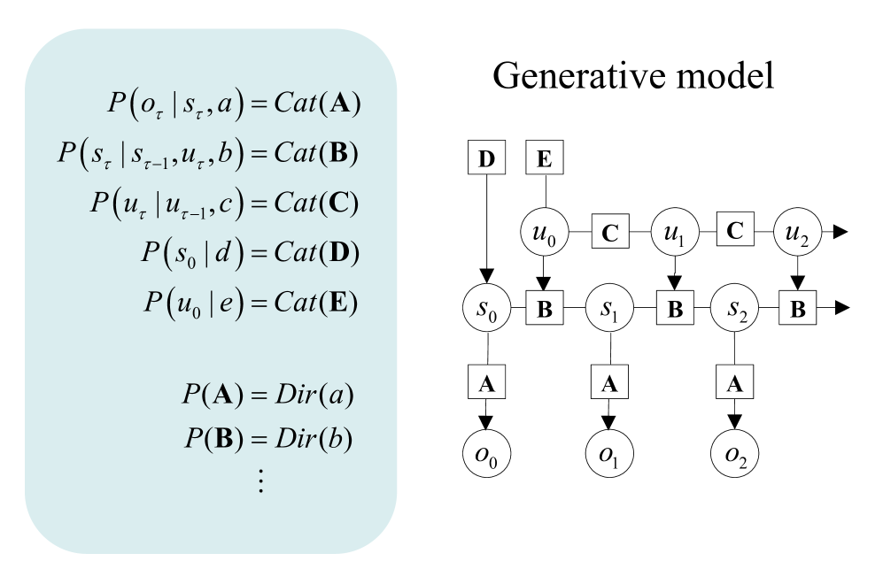### The generative model Figure 2 provides a schematic overview of the generative model used for the simulations considered in this paper. Outcomes at any particular time depend upon hidden states, while transitions among hidden states depend upon paths. Note that paths are random variables, in the sense that a particle can have both a position (i.e., a state) and momentum (i.e., a path). Paths may or may not depend upon action. The resulting POMDP is specified by a set of tensors. The first set of parameters, denoted $A$ , maps from hidden states to outcome modalities; for example, exteroceptive (e.g., visual) or proprioceptive (e.g., eye position) modalities. These parameters encode the likelihood of an outcome given their hidden causes. The second set $B$ prescribes transitions among the hidden states of a factor, under a particular path. Factors correspond to different kinds of causes; e.g., the location versus the class of an object. The remaining tensors encode prior beliefs about paths $C$ , and initial states $D$ . The tensors—encoding probabilistic mappings or contingencies—are generally parameterised as Dirichlet distributions, whose sufficient statistics are concentration parameters or Dirichlet counts. These count the number of times a particular combination of states or outcomes has been inferred. We will focus on learning the likelihood model, encoded by Dirichlet counts, $\boldsymbol{a}$ . <details> <summary>x2.png Details</summary>  ### Visual Description \n ## Probabilistic Generative Model Diagram ### Overview The image displays a technical diagram of a probabilistic generative model, split into two primary sections. On the left, within a light blue rounded rectangle, is a set of mathematical equations defining the model's probability distributions. On the right is a corresponding graphical model (a Bayesian network) titled "Generative model," which visually represents the dependencies between variables over discrete time steps. The diagram illustrates a sequential process involving observations, latent states, and control inputs. ### Components/Axes The diagram is composed of two main components: 1. **Left Panel (Mathematical Definitions):** Contains a list of probability distributions. 2. **Right Panel (Graphical Model):** A directed acyclic graph showing variables as nodes and dependencies as arrows. The graph is organized into three horizontal layers over time steps (τ = 0, 1, 2,...). **Graphical Model Node Types:** * **Circular Nodes:** Represent random variables. * `o_τ`: Observation at time τ. * `s_τ`: Latent state at time τ. * `u_τ`: Control input or action at time τ. * **Square Nodes:** Represent fixed parameters or hyperparameters. * `A`, `B`, `C`, `D`, `E`: Parameter matrices/vectors for the categorical distributions. * `a`, `b`, `c`, `d`, `e`: Hyperparameters for the Dirichlet priors (implied by the equations). **Graphical Model Flow & Connections:** * **Vertical Flow (Generative Process):** Arrows point downward, indicating the direction of conditional dependence in the generative process. * Parameters `D` and `E` influence the initial state `s_0` and initial input `u_0`, respectively. * Parameters `C` connect consecutive control inputs (`u_τ-1` to `u_τ`). * Parameters `B` connect consecutive states (`s_τ-1` to `s_τ`) and are also influenced by the current control input `u_τ`. * Parameters `A` connect the current state `s_τ` to the observation `o_τ`. * **Horizontal Flow (Time):** The model unfolds over time from left (τ=0) to right (τ=1, 2,...), indicated by the sequence of `u`, `s`, and `o` nodes and the right-pointing arrows from `u_2` and `s_2`. ### Detailed Analysis **1. Mathematical Equations (Left Panel):** The equations define a hierarchical Bayesian model with categorical observations and Dirichlet priors. * `P(o_τ | s_τ, a) = Cat(A)`: The observation `o_τ` at time τ is drawn from a Categorical distribution parameterized by `A`, conditioned on the current state `s_τ` and some fixed parameter `a`. * `P(s_τ | s_τ-1, u_τ, b) = Cat(B)`: The state `s_τ` transitions from the previous state `s_τ-1` and current input `u_τ` via a Categorical distribution parameterized by `B`, with hyperparameter `b`. * `P(u_τ | u_τ-1, c) = Cat(C)`: The control input `u_τ` depends on the previous input `u_τ-1` through a Categorical distribution parameterized by `C`, with hyperparameter `c`. * `P(s_0 | d) = Cat(D)`: The initial state `s_0` is drawn from a Categorical distribution parameterized by `D`, with hyperparameter `d`. * `P(u_0 | e) = Cat(E)`: The initial control input `u_0` is drawn from a Categorical distribution parameterized by `E`, with hyperparameter `e`. * `P(A) = Dir(a)`, `P(B) = Dir(b)`, `⋮`: The parameters `A`, `B`, etc., themselves have Dirichlet prior distributions with hyperparameters `a`, `b`, etc. The ellipsis (`⋮`) indicates this pattern continues for parameters `C`, `D`, and `E`. **2. Graphical Model (Right Panel):** The diagram visually instantiates the equations for the first three time steps (τ=0, 1, 2). * **Initial Conditions (Top-Left):** Nodes `D` and `E` (squares) have arrows pointing to `s_0` and `u_0` (circles), respectively, representing the initial state and input distributions. * **Time Step τ=0:** The initial state `s_0` and input `u_0` are connected via a `B` parameter node to generate the next state `s_1`. The state `s_0` also connects via an `A` parameter node to generate observation `o_0`. * **Time Step τ=1:** The state `s_1` and input `u_1` (which depends on `u_0` via `C`) connect via `B` to generate `s_2`. The state `s_1` connects via `A` to generate observation `o_1`. * **Time Step τ=2:** The pattern continues, with `s_2` and `u_2` leading to a subsequent state (implied by the right-pointing arrow from `s_2`), and `s_2` generating observation `o_2` via `A`. * **Control Input Chain:** The `u` nodes (`u_0`, `u_1`, `u_2`) are connected horizontally by `C` parameter nodes, showing the autoregressive dependency of inputs. ### Key Observations 1. **Recursive Structure:** The model exhibits a clear recursive, state-space structure common in hidden Markov models (HMMs) and control systems. The state `s_τ` is a Markov blanket, summarizing the past to predict the future. 2. **Dual Dependency for States:** The state transition `P(s_τ | ...)` depends on both the previous state (`s_τ-1`) and the current control input (`u_τ`), making it a controlled Markov process. 3. **Separate Input Dynamics:** The control inputs `u_τ` have their own autoregressive dynamics (`P(u_τ | u_τ-1, c)`), modeled independently of the state. 4. **Parameter Sharing:** The same parameter nodes (`A`, `B`, `C`) are reused across all time steps, indicating parameter sharing and a stationary process (the rules don't change over time). 5. **Bayesian Hierarchy:** The model is fully Bayesian, with Dirichlet priors on the categorical parameters, allowing for uncertainty quantification and learning from data. ### Interpretation This diagram defines a **controlled, autoregressive state-space model** with categorical variables. It is a generative recipe for creating sequences of observations (`o_0, o_1, o_2,...`) by first sampling initial conditions, then recursively sampling states and inputs. * **What it represents:** This is a classic model for **sequential decision-making** or **robotics**. The `u` variables could be actions taken by an agent, the `s` variables are the hidden states of the environment, and the `o` variables are the agent's noisy perceptions. The model can be used for planning (generating action sequences) or learning (inferring states and parameters from observed data). * **Relationships:** The core relationship is that the observable world (`o`) is generated from a hidden state (`s`), which itself evolves based on its own history and the agent's actions (`u`). The agent's actions also have their own momentum or policy (`C`). * **Notable Anomaly/Feature:** The inclusion of explicit parameters `D` and `E` for the initial conditions is noteworthy. It formally separates the initialization process from the recursive dynamics, which is crucial for clear model specification. * **Underlying Logic:** The use of Categorical distributions suggests the state, action, and observation spaces are discrete. The Dirichlet priors are conjugate to the Categorical likelihood, which simplifies mathematical inference (e.g., using Gibbs sampling). The ellipsis (`⋮`) implies the model is extensible to more parameters or time steps. **In essence, this image provides a complete specification for a probabilistic program that can generate synthetic time-series data mimicking a controlled, discrete system, or conversely, be used to infer the hidden causes of real-world sequential data.** </details> Figure 2: Generative models as agents. A generative model specifies the joint probability of observable consequences and their hidden causes. Usually, the model is expressed in terms of a likelihood (the probability of consequences given their causes) and priors (over causes). When a prior depends upon a random variable it is called an empirical prior. Here, the likelihood is specified by a tensor $A$ , encoding the probability of an outcome under every combination of states ( $s$ ). The empirical priors pertain to transitions among hidden states, $B$ , that depend upon paths ( $u$ ), whose transition probabilities are encoded in $C$ . $E$ specifies the empirical prior probability of each path. The subscripts in this graphic pertain to time. The generative model in Figure 2 means that outcomes are generated as follows: first, a policy is selected using a softmax function of expected free energy. Sequences of hidden states are generated using the probability transitions specified by the selected combination of paths (i.e., policy). Finally, these hidden states generate outcomes in one or more modalities. Perception or inference about hidden states (i.e., state estimation) corresponds to inverting a generative model, given a sequence of outcomes, while learning corresponds to updating model parameters. Perception therefore corresponds to updating beliefs about hidden states and paths, while learning corresponds to accumulating knowledge in the form of Dirichlet counts. The requisite expectations constitute the sufficient statistics $(s,u,a)$ of posterior beliefs $Q(s,u,a)=Q_s(s)Q_u(u)Q_a(a)$ . The implicit factorisation of this approximate posterior effectively partitions model inversion into inference, planning, and learning. ### Variational free energy and inference In variational Bayesian inference (a form of approximate Bayesian inference), model inversion entails the minimisation of variational free energy with respect to the sufficient statistics of approximate posterior beliefs. This can be expressed as follows, where, for clarity, we will deal with a single factor, such that the policy (i.e., combination of paths) becomes the path, $π=u$ . Omitting dependencies on previous states, we have for model $m$ : $$ \displaystyle Q≤ft(s_τ,u_τ,a\right) \displaystyle=\arg\min_QF \displaystyle F \displaystyle=E_Q[\ln\underbrace{Q≤ft(s_τ,u_τ,a\right)} _posterior -\ln\underbrace{P≤ft(o_τ\mid s_τ,u_τ,a \right)}_likelihood -\ln\underbrace{P≤ft(s_τ,u_τ,a\right) }_prior ] \displaystyle=\underbrace{D_KL≤ft[Q≤ft(s_τ,u_τ,a\right)\|P ≤ft(s_τ,u_τ,a\mid o_τ\right)\right]}_divergence - \underbrace{\ln P≤ft(o_τ\mid m\right)}_log evidence \displaystyle=\underbrace{D_KL≤ft[Q≤ft(s_τ,u_τ,a\right)\|P ≤ft(s_τ,u_τ,a\right)\right]}_complexity -\underbrace{ E_Q≤ft[\ln P≤ft(o_τ\mid s_τ,u_τ,a\right)\right]} _accuracy \tag{1} $$ Because the (KL) divergences cannot be less than zero, the penultimate equality means that free energy is minimised when the (approximate) posterior is equal to the true posterior. At this point, the free energy is equal to the negative log evidence for the generative model [35]. This means minimising free energy is mathematically equivalent to maximising model evidence, which is, in turn, equivalent to minimising the complexity of accurate explanations for observed outcomes. Planning emerges under active inference by placing priors over (controllable) paths to minimise expected free energy [41]: $$ \displaystyle G(u) \displaystyle=E_Q_{u}≤ft[\ln Q≤ft(s_τ+1,a\mid u\right)-\ln Q ≤ft(s_τ+1,a\mid o_τ+1,u\right)-\ln P≤ft(o_τ+1\mid c\right)\right] \displaystyle=-\underbrace{E_Q_{u}≤ft[\ln Q≤ft(a\mid s_τ+1 ,o_τ+1,u\right)-\ln Q(a\mid s_τ+1,u)\right]}_expected information gain (learning) - \displaystyle \underbrace{E_Q_{u}≤ft[\ln Q≤ft(s_τ+ 1\mid o_τ+1,u\right)-\ln Q≤ft(s_τ+1\mid u\right)\right]}_ expected information gain (inference) \underbrace{-E_Q_{u}≤ft[ \ln P≤ft(o_τ+1\mid c\right)\right]}_expected cost \displaystyle=-\underbrace{E_Q_{u}≤ft[D_KL≤ft[Q≤ft(a\mid s_ {τ+1},o_τ+1,u\right)\|Q(a\mid s_τ+1,u)\right]\right]}_ novelty + \displaystyle \underbrace{D_KL≤ft[Q≤ft(o_τ+1\mid u\right) \|P≤ft(o_τ+1\mid c\right)\right]}_risk \underbrace{-E _Q_{u}≤ft[\ln Q≤ft(o_τ+1\mid s_τ+1,u\right)\right]}_ ambiguity \tag{3} $$ Here, the posterior predictive distribution over parameters, hidden states and outcomes at the next time step, under a particular path, is defined as follows: | | $\displaystyle Q_u$ | $\displaystyle=Q≤ft(o_τ+1,s_τ+1,a\mid u\right)$ | | | --- | --- | --- | --- | One can also express the prior over the parameters in terms of an expected free energy, where, marginalising over paths: $$ \displaystyle P(a) \displaystyle=σ(-G) \displaystyle G(a) \displaystyle=E_Q_{a}[\ln P(s\mid a)-\ln P(s\mid o,a)-\ln P(o\mid c)] \displaystyle=-\underbrace{E_Q_{a}[\ln P(s\mid o,a)-\ln P(s\mid a)] }_expected information gain \underbrace{-E_Q_{a}[\ln P(o \mid c)]}_expected cost \displaystyle=-\underbrace{E_Q_{a}≤ft[D_KL[P(o,s\mid a)\|P(o \mid a)P(s\mid a)]\right.}_mutual information \underbrace{-E _Q_{a}[\ln P(o\mid c)]}_expected cost \tag{5} $$ where $Q_a=P(o|s,a)P(s|a)=P(o,s|a)$ is the joint distribution over outcomes and hidden states, encoded by the Dirichlet parameters, $a$ , and $σ(·)$ is the softmax function. Note that the Dirichlet parameters encode the mutual information, in the sense that they implicitly encode the joint distribution over outcomes and their hidden causes. When normalising each column of the $a$ tensor, we recover the likelihood distribution (as in Figure 2); however, we could normalise over every element, to recover a joint distribution. As discussed above, expected free energy can be regarded as a universal objective function that augments mutual information with expected costs or constraints. Constraints — parameterised by $c$ — reflect the fact that we are dealing with open systems with characteristic outcomes. This allows an optimal trade-off between exploration and exploitation, that can be read as an expression of the constrained maximum entropy principle that is dual to the free energy principle [19]. Alternatively, it can be read as a constrained principle of maximum mutual information or minimum redundancy [42, 43, 44, 45]. In machine learning, this kind of objective function underwrites disentanglement [46, 47], and generally leads to sparse representations [48, 45, 49, 50]. When comparing the expressions for expected free energy in Equation 2 with variational free energy in Equation 1, the expected divergence becomes expected information gain. Expected information gain about the parameters and states are sometimes associated with distinct epistemic affordances; namely, novelty and salience, respectively [51]. Similarly, expected log evidence becomes expected value, where value is the logarithm of prior preferences. The last equality in Equation 2 provides a complementary interpretation; in which the expected complexity becomes risk, while expected inaccuracy becomes ambiguity. There are many special cases of minimising expected free energy. For example, maximising expected information gain maximises (expected) Bayesian surprise [52], in accord with the principles of optimal (Bayesian) experimental design [53]. This resolution of uncertainty is related to artificial curiosity [54, 55] and speaks to the value of information [56]. Expected complexity or risk is the same quantity minimised in risk sensitive or KL control [57, 58], and underpins (free energy) formulations of bounded rationality based on complexity costs [59, 60] and related schemes in machine learning; e.g., Bayesian reinforcement learning [61]. More generally, minimising expected cost subsumes Bayesian decision theory [62]. <details> <summary>x3.png Details</summary>  ### Visual Description ## Technical Diagram: Inductive Planning Process ### Overview The image is a composite technical diagram illustrating a mathematical framework for "Inductive planning." It consists of three interconnected panels: a left panel containing a set of equations, a central panel visualizing a sequence of states and their relationships, and a right panel displaying a specific matrix structure. Red arrows are used to link conceptual elements across the panels. ### Components/Axes **Left Panel (Equations):** * **Title:** "Inductive planning" * **Equations (transcribed precisely):** 1. `I₀ = h` 2. `Iₙ₊₁ = B̃ᵀ ⊙ Iₙ` 3. `B̃ = B > ε : ∃u` 4. `pₙ = Iₙ ⊙ s_τ` 5. `m = arg maxₙ pₙ < sup p` 6. `H = ln ε · Iₘ ⊙ s_{τ+1}` 7. `P(u) = σ(-G - H)` **Central Panel (State Sequence Visualization):** * **Axes:** * Horizontal axis (bottom): Labeled `n`, with tick marks at 5, 10, 15, 20, 25, 30. An arrow below points left with the label `←future` and right with the label `past→`. * Vertical axis (left): Labeled `m`, with tick marks from 10 to 100 in increments of 10. * **Key Elements:** * A vertical black bar on the far left labeled `s_τ`. * A large central matrix labeled `I = [I₀, I₁, ..., I_N]`. This matrix is primarily black with a white, jagged, horizontal pattern running through it. * A horizontal red arrow originates from the `s_τ` bar at approximately `m=20` and points right into the `I` matrix. * A vertical red dashed line runs through the `I` matrix at approximately `n=12`. It is labeled `Iₘ`. * A horizontal red arrow originates from the top of the `Iₘ` line and points upward to a small horizontal bar chart. * A small horizontal bar chart at the top is labeled `pₙ = Iₙ ⊙ s_τ`. Its horizontal axis has tick marks from 5 to 30. * A label `h` with a red arrow points to the `I` matrix at approximately `m=65, n=0`. **Right Panel (Matrix Plot):** * **Title/Label:** `B̃ = B > ε : ∃u` * **Axes:** * Horizontal axis (bottom): Tick marks at 20, 40, 60, 80, 100. * Vertical axis (left): Tick marks at 10, 20, 30, 40, 50, 60, 70, 80, 90, 100. * **Content:** A square, black-and-white matrix plot. It shows a strong white diagonal line from the top-left to bottom-right corner, accompanied by several parallel, fainter white lines offset from the main diagonal. ### Detailed Analysis The diagram visually maps the mathematical operations defined in the left panel onto the structures in the central and right panels. 1. **Equation Flow:** The process begins with an initial state `I₀ = h`. The state is iteratively updated via `Iₙ₊₁ = B̃ᵀ ⊙ Iₙ`, where `B̃` is a thresholded version of a matrix `B` (defined as `B̃ = B > ε : ∃u`). The right panel visualizes this `B̃` matrix, showing a banded diagonal structure. 2. **State Evaluation:** At each step `n`, a value `pₙ` is computed as the dot product (`⊙`) of the current state `Iₙ` and a target or sensory vector `s_τ`. The top bar chart in the central panel visualizes these `pₙ` values across `n`. 3. **State Selection:** The index `m` is selected as the argument maximizing `pₙ`, subject to the constraint that `pₙ` is less than the supremum of `p` (`m = arg maxₙ pₙ < sup p`). This selected state `Iₘ` is highlighted by the vertical red dashed line in the central matrix `I`. 4. **Heuristic Computation:** A heuristic `H` is computed using the selected state `Iₘ` and the *next* sensory input `s_{τ+1}`: `H = ln ε · Iₘ ⊙ s_{τ+1}`. 5. **Policy Output:** Finally, a policy or probability `P(u)` is generated by passing the negative sum of two terms (`G` and `H`) through a sigmoid function `σ`: `P(u) = σ(-G - H)`. ### Key Observations * **Spatial Linking:** The red arrows create a clear visual narrative: the sensory input `s_τ` influences the state matrix `I`; a specific state `Iₘ` is selected based on the computed `pₙ` values; this selection then feeds into the calculation of `H`. * **Matrix Structure:** The `B̃` matrix in the right panel is not random. Its strong diagonal and parallel off-diagonals suggest a structured, possibly time-lagged or spatially-localized, transition or influence matrix. * **State Matrix Texture:** The central `I` matrix is not uniform. The white, jagged horizontal pattern indicates that the state representation is sparse or has a specific, non-random structure across the `m` dimension for each time step `n`. * **Temporal Direction:** The axis labels `←future` and `past→` indicate that increasing `n` corresponds to moving backward in time (toward the past), which is a common convention in some planning or sequence modeling contexts. ### Interpretation This diagram outlines a computational framework for inductive planning, likely in an AI or cognitive modeling context. The process involves: 1. **Maintaining a Belief State (`I`):** A structured internal representation (`I`) is updated over time (`n`) based on a transition model (`B̃`). 2. **Evaluating Against Goals:** The current belief state is continuously evaluated (`pₙ`) against a target or sensory goal (`s_τ`). 3. **Selecting a Reference Point:** A specific past state (`Iₘ`) that best matched the goal (but was not a perfect match, due to the `< sup p` constraint) is selected. This acts as an inductive reference point. 4. **Generating a Heuristic:** Using this reference state and *new* sensory information (`s_{τ+1}`), a heuristic `H` is computed. This heuristic likely guides future planning or action selection. 5. **Producing a Policy:** The final output is a policy `P(u)`, which is a function of this learned heuristic `H` and another term `G` (not defined in the diagram, possibly a cost or prior). The core idea appears to be using past experiences (stored in `I` and selected via `Iₘ`) to inductively generate heuristics for decision-making in new, but related, situations. The structured nature of `B̃` and `I` suggests the model exploits specific temporal or spatial regularities in the problem domain. 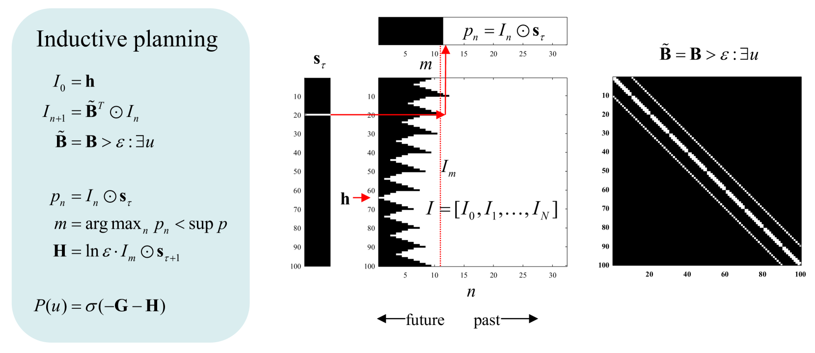</details> Figure 3: Inductive Planning. This figure provides an overview of inductive planning used in this paper. The left panel provides the expressions used to induce which subsequent states do and do not contain paths to some intended end state, encoded by a one hot vector $h$ . The central panel illustrates this induction graphically, where vectors and matrices are shown in image format (black equals zero or false and white equals one or true). Working down the equalities in the left panel, we first initialise a logical vector of states, $I$ , to the intended state $h$ . Recursively, we evaluate all the states from which the previous state can be accessed (a state can be accessed if the probability of transitioning from an adjacent state is larger than $ε$ ). Because this recursive induction works backwards in time, the allowable transition matrix is transposed. Having induced the reverse history of states—that contain paths to the intended state—one can then evaluate the length of the shortest path to the intended state. This depends upon posterior beliefs about the current state. In the example shown on the left, we are currently in state $20$ , which means that the shortest path to the intended state (state $64$ ) is $12$ time steps. This tells us that if we are pursuing the shortest path then there are certain states we need to avoid—from which the intended state cannot be reached. These states are encoded by the logical vector I at the next time step; namely, the last time before the probability $p$ of being on a path to the intended state reaches its supremum. Because the eligible states can only increase—as we move backwards in time—this probability can only increase, until all states are eligible (or there are no further eligible states). The first time that the probability reaches its supremum tells us where we are on the path to our intended state and, crucially, the ineligible states at the next time step. We now know the states to avoid at the next time step. If ineligible states are precluded, the next state must be on the path to the intended state. Ineligible states can be assigned a high cost (here, the log of a small value) to evaluate the expected cost incurred by each policy, using its predictive posterior over states (see Figure 2). Finally, we can supplement the expected free energy, $G$ of each policy with the ensuing inductive cost, $H$ . In principle, this guarantees the selection of paths or policies that lead to the intended state, provided that state can be reached. The example shown on the right is taken from the maze navigation task described later. For clarity, this example only considers a single factor. The mathematical expressions use the notation of Figure 2: The dotted red line indicates the logical vector encoding which of the $100$ states will lead to the intended state at the next time point; here, $11$ time steps from the intended state (indicated with a small red arrow). ## 3 Inductive Planning What we call inductive planning—in this setting—recalls the notion of backwards induction in dynamic programming and related schemes [63, 25, 30, 23, 26, 64, 27]. In this form of inference, precise beliefs about state transitions are leveraged to rule out actions that are inconsistent with the attainment of future goals, defined in belief or state space as a final (or intended) state. This is a limiting case of inductive (Bayesian) inference [65, 66, 67] in which the very high precision of beliefs about final or intended states allows one to use logical operators in place of tensor operations; thereby vastly simplifying computations. In brief, we will use this simplification to furnish constraints on action selection that inherit from priors over intended states in the future. Active inference rests on priors that place constraints on paths or trajectories through state space. For example, a sparse prior preference with knowledge only about the final state warrants deep planning to demonstrate intentional behaviour [27]. One can either specify these constraints in terms of states that are unlikely to traversed, or in terms of the final state. In other words, the agent may, a priori, believe it will navigate state space in a way that avoids unlikely or surprising outcomes, or that it will reach some final destination (in state space, not outcome space), irrespective of the path taken. These are distinct kinds of constraints. The first is implemented by $c$ , in terms of the cost or constraints that apply during the entire path. We now introduce another prior or constraint $h$ , over the final state. The priors, $d$ and $h$ play reciprocal roles; in the sense they specify prior beliefs about the initial and final states, respectively. Backwards induction now follows simply from this prior; provided it is specified sufficiently precisely. We will refer to these final states as intended states While $c$ , $d$ , and $h$ are usually hard coded, they can be learnt very efficiently, for example using Z-learning for certain classes of MDPs [68, 27]. The basic idea is that although we may be uncertain about the next latent state, we can be certain about which states cannot be accessed from the current state. This means we can use induction to identify subsequent states that cannot be on a path to an intended state; thereby rendering actions—(i.e., state transitions) to those ineligible, ’dead-end’ states—highly unlikely (assuming that we are on a path to an intended state). The requisite induction goes as follows: Imagine that we know our current state and that we will be in a certain (intended) state in the future. Imagine further that we know all possible transitions, afforded by action, among states. This means we can identify all the states from which the intended state is accessible. We can now repeat this and identify all the states from which the eligible states at the penultimate time point can be accessed, and so on. We now repeat this recursively—moving backwards in time—until our current state becomes eligible. At this point, we select an action that precludes ineligible states at the preceding point in backwards time (or next point in forwards time), bringing us one step closer to the intended state. We now repeat the backwards induction, until we arrive at the intended state, via the shortest path. This backwards induction is computationally cheap because it entails logical operations on a sparse logical tensor, encoding allowable state transitions. Figure 3 provides a pseudocode and graphical abstraction based upon the MATLAB scripts implementing this inductive logic. For clarity, we have assumed a single factor and that there are no constraints on the paths, other than those specified by a one hot vector $h$ , specifying the agent’s intended states In our MATLAB implementation of inductive planning, constraints due to prior preferences in outcome space are accommodated by precluding transitions to costly states during construction of the logical matrix encoding possible or true transitions. Furthermore, the implementation deals with multiple factors using appropriate tensor products. Finally, when multiple intended states are supplied, the nearest state is chosen for induction; where nearest is defined in terms of the number of timesteps required to access an intended state.. Note that this is not vanilla backwards induction. It is simply a way of placing precise priors on paths that render certain paths—that cannot access an intended state—highly unlikely. The requisite priors complement expected free energy in the following sense (see Figure 3): inductive priors over policies, $H$ are derived from priors over intended states $h$ , while the priors over policies scored by expected free energy, $G$ inherit from priors over preferred outcomes $c$ . This distinction is important because it means that this kind of reasoning—and intentional behaviour—can only manifest under precise beliefs about latent states. For example, a baby (or unexplainable neural network) could not, by definition, act intentionally because it does not have a precise generative model of latent states (or any mechanism to specify intended states). We will return to prerequisites for inductive planning in the discussion. In summary, inductive planning propagates constraints backwards in time to provide empirical priors for planning as inference in the usual way. This means that—within the constraints afforded by such planning—actions will still be chosen that maximise expected information gain and any constraints encoded by $c$ . In this sense, the inductive part of this inference scheme can be regarded as providing a constrained expected free energy, which winnows trajectories through state space to paths of least action. An equivalent and alternative perspective is that inductive planning furnishes an empirical prior over policies. When intended states are conditioned on some context—inferred by a supraordinate (hierarchical) level—one has the opportunity to learn intended states and, effectively, make planning habitual. In this setting, the implicit Dirichlet counts in $h$ , could be regarded as accumulating habitual courses of action that are learned as empirical priors in hierarchical models. We will pursue this elsewhere. In what follows, we focus on the distinction between sentient behaviour—based upon expected free energy—and intentional behaviour—based upon inductive priors. ## 4 Pong Revisited In this section, we first simulate ’mere’ sentient Behaviour and then examine the qualitative differences in behaviour when adding inductive constraints. Specifically, we simulate the in vitro experiments reported in [1], using both an abductive and an inductive agent. The first has no intended goals, and stands in for a naïve neuronal culture; the second has as set of intended states: the ones where the paddle hits upcoming balls. As environments, we use Pong of two different sizes, that reflect two different difficulties: $5× 6$ (easy), and $8× 4$ (hard). The results show that while the simulated in vitro agent is able to fluently play in the easy environment, it struggles in the harder one. The inductive agent, on the other hand, can master the harder environment in less than three minutes of (simulated) game time. 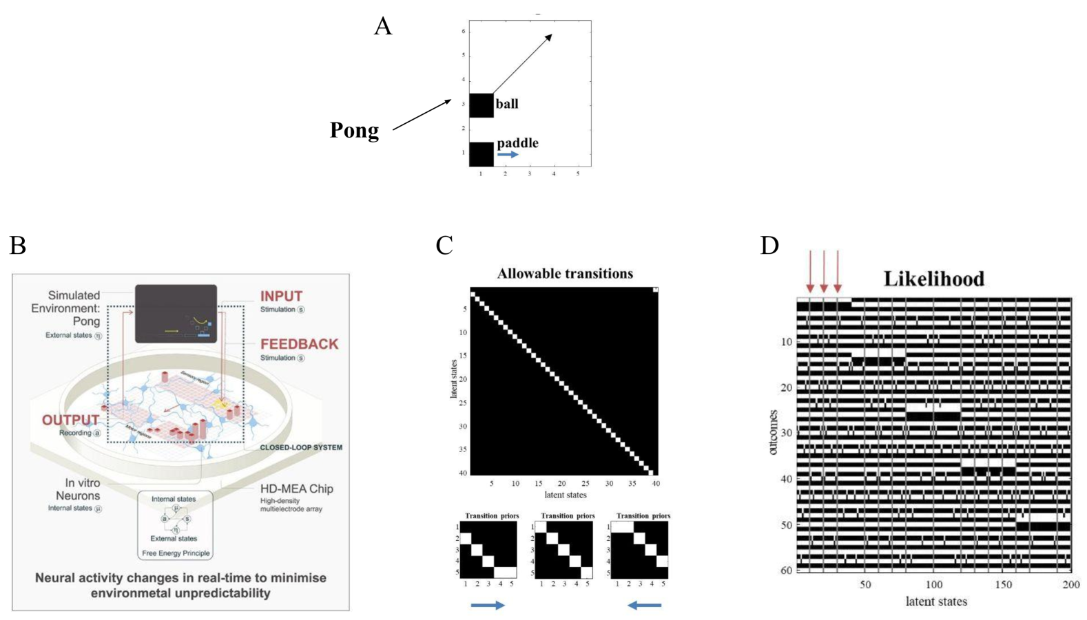In the in vitro experiments, certain cells were stimulated depending upon the configuration of a virtual game of Pong, constituted by the position of a paddle and a ball bouncing around a bounded box. Other recording electrodes were used to drive the paddle, thereby closing the sparse coupling between the neuronal network and the computer network simulating the game of Pong (see Figure 4). Typically, in these experiments, after a few minutes of exposure to the game, short rallies of ball returns emerge. To emulate this setup, we created a generative process (i.e., a hard-coded representation of the dynamics of external states) in which a ball bounced around a box at $45$ degrees. The lower boundary contained a paddle that could be moved to the right or left. The size of the box was $5× 6$ units, where the ball moved one unit up or down (and right or left) at every time point. The (one unit wide) paddle could be moved left or right by one unit at every time point. In the in vitro experiments, whenever the agent missed the ball, either white noise or no stimulation was applied to the sensory electrodes; otherwise, the game remained in the play. We simulated this by supplying random input to all sensory channels whenever the ball failed to contact the paddle on the lower boundary. The (sensory) outcomes of the POMDP comprised $30$ sensory channels that could be on or off. These can be thought of as pixels in a simple Atari-like game. The latent states were modelled as one long orbit, by equipping the generative model with a transition matrix that moved from one state to the next (with circular boundary conditions) for a suitably long sequence of state transitions (here, $40$ ). The generative model was equipped with a second factor with three controllable paths. This factor moved the paddle one unit to the right or left (or no movement). However, the (implicit) agent knew nothing more about its world and, in particular, had no notion that the second factor endowed it with control over the paddle. This was because the likelihood tensors mapping from the two latent factors to the outcomes were populated with small and uniform Dirichlet counts (i.e., concentration parameters of $1/32$ ). In other words, our naïve generative model could, in principle, model any given world (providing this world has a limited number of states that are revisited systematically). Figure 4 shows the setup of this paradigm and the parameters of the generative model learned after $512$ time steps. <details> <summary>x4.png Details</summary>  ### Visual Description \n ## Multi-Panel Scientific Figure: Neural Closed-Loop System for Pong ### Overview This image is a composite scientific figure consisting of four panels (A, B, C, D) illustrating a closed-loop system where *in vitro* neural activity on a high-density microelectrode array (HD-MEA) chip interacts with a simulated Pong game environment. The system is framed within the Free Energy Principle, where neural activity changes in real-time to minimize environmental unpredictability. ### Components/Axes **Panel A (Top Center):** * **Title/Label:** "A" (top-left of panel). * **Diagram:** A simplified schematic of the game Pong. * **Text Elements:** * "Pong" (with an arrow pointing to the diagram). * "ball" (label next to a black square). * "paddle" (label next to a black rectangle). * **Axes:** The diagram is plotted on a 2D grid. * **X-axis:** Numbered from 1 to 5. * **Y-axis:** Numbered from 1 to 6. * **Visual Elements:** A black square ("ball") at approximately (1, 3) with an arrow pointing diagonally up and right. A black rectangle ("paddle") at approximately (1, 1) with a blue arrow pointing right. **Panel B (Bottom Left):** * **Title/Label:** "B" (top-left of panel). * **Diagram Type:** System architecture diagram for a "CLOSED-LOOP SYSTEM". * **Text Elements & Components (Spatially Organized):** * **Top Left:** "Simulated Environment: Pong" with sub-label "External states (η)". * **Top Right:** "INPUT" in red, with "Stimulation (S)" below it. * **Center:** An illustration of a petri dish containing a neural network, labeled "In vitro Neurons" with sub-label "Internal states (μ)". * **Center Right:** "FEEDBACK" in red, with "Stimulation (S)" below it. * **Bottom Left:** "OUTPUT" in red, with "Recording (R)" below it. * **Bottom Right:** "HD-MEA Chip" with sub-label "High-density multielectrode array". * **Bottom Center:** A box labeled "Free Energy Principle" containing a diagram with "Internal states (μ)" and "External states (η)". * **Bottom Caption:** "Neural activity changes in real-time to minimise environmental unpredictability". * **Flow/Arrows:** Dotted red lines show a loop: from the Simulated Environment (Pong) -> INPUT (Stimulation) -> Neurons -> OUTPUT (Recording) -> back to the Simulated Environment. Solid black lines connect the neurons to the HD-MEA Chip and the Free Energy Principle box. **Panel C (Bottom Center):** * **Title/Label:** "C" (top-left of panel). * **Chart Type:** Heatmap. * **Main Title:** "Allowable transitions". * **Axes:** * **X-axis:** "latent states", numbered from 5 to 40 in increments of 5. * **Y-axis:** "latent units", numbered from 5 to 40 in increments of 5. * **Data Pattern:** A black background with a diagonal line of white squares running from the top-left (low latent state/unit) to the bottom-right (high latent state/unit). This indicates a one-to-one mapping or allowable transition between corresponding latent states and units. * **Subplots (Below Main Heatmap):** * Three smaller heatmaps, each titled "Transition priors". * Each has axes numbered 1 to 5. * Each shows a 5x5 black grid with a single white square in a different position, forming a diagonal pattern across the three plots. * **Arrows:** A blue arrow pointing right is below the left subplot. A blue arrow pointing left is below the right subplot. **Panel D (Bottom Right):** * **Title/Label:** "D" (top-left of panel). * **Chart Type:** Heatmap. * **Main Title:** "Likelihood". * **Axes:** * **X-axis:** "latent states", numbered from 50 to 200 in increments of 50. * **Y-axis:** "outcomes", numbered from 10 to 60 in increments of 10. * **Data Pattern:** A black background with a complex pattern of horizontal white stripes of varying lengths and positions. The stripes are denser and more continuous in the lower half of the chart (outcomes 30-60) and more fragmented in the upper half (outcomes 10-30). * **Annotations:** Three red arrows point downward from the top edge of the chart, aligned approximately with latent states 20, 40, and 60. ### Detailed Analysis * **Panel A:** Defines the external task. The ball's trajectory (arrow) and paddle's movement direction (blue arrow) are the key dynamic elements. * **Panel B:** Details the experimental loop. The "Internal states (μ)" of the neurons are influenced by "Stimulation (S)" (INPUT/FEEDBACK) from the game and produce "Recording (R)" (OUTPUT) that affects the game. The Free Energy Principle is presented as the theoretical framework governing this interaction. * **Panel C:** The main heatmap shows a strict, diagonal "allowable transitions" matrix, suggesting a highly structured or constrained relationship between latent states and latent units. The "Transition priors" subplots likely show specific, simple transition rules (e.g., state 1->2, 2->3, etc.). * **Panel D:** The "Likelihood" heatmap shows the probability (indicated by white) of various "outcomes" given different "latent states". The pattern is not uniform; certain outcome bands (e.g., around 40-50) are highly likely across many latent states, while others are more sporadic. The red arrows may highlight specific latent states of interest. ### Key Observations 1. **Structured Constraint:** Panel C's perfect diagonal indicates a non-random, possibly engineered or learned, one-to-one mapping in the system's internal dynamics. 2. **Outcome Variability:** Panel D shows that the likelihood of outcomes is highly dependent on the latent state, with clear bands of high and low probability. 3. **Theoretical Framework:** The explicit inclusion of the "Free Energy Principle" in Panel B is a key conceptual component, framing the entire experiment as a process of minimizing surprise or prediction error. 4. **Real-Time Adaptation:** The caption in Panel B emphasizes the *real-time* nature of the neural adaptation, which is central to the closed-loop concept. ### Interpretation This figure describes an experiment designed to test if a biological neural network (in vitro neurons) can learn to control a simple external environment (Pong) by adhering to the Free Energy Principle. * **What it demonstrates:** The setup aims to show that neural activity isn't just a passive recorder but an active inference engine. By receiving feedback (stimulation) from the game state and generating output (recordings) that move the paddle, the network attempts to build an accurate internal model (latent states) of the external world (the ball's movement) to minimize long-term prediction error (environmental unpredictability). * **Relationship between elements:** Panel A is the external world. Panel B is the embodied interface between biology and that world. Panels C and D likely represent the internal, learned model of the system. Panel C's diagonal suggests the network may have developed a clean, segregated representation where specific internal units track specific game states. Panel D shows how these internal representations (latent states) map to observable game outcomes, revealing the network's predictive model. * **Anomalies/Notable Points:** The stark contrast between the clean, diagonal structure in Panel C and the complex, banded pattern in Panel D is striking. It suggests that while the internal state transitions may be simple and orderly, the mapping from those states to external outcomes is rich and probabilistic. The red arrows in Panel D may point to latent states where the outcome likelihood distribution changes significantly, possibly corresponding to critical events in the game (e.g., the ball crossing a midpoint). </details> Figure 4: Learning the world of Pong. Panel $A$ : Setup used in the simulations. In brief, the generative process modelled a ball bouncing around inside a bounding box, with a movable paddle on the lower boundary. The $(5× 6=)30$ locations or pixels provided outputs with two states (black or white) that were subsequently learned via a likelihood mapping to $40$ latent states. The agent was equipped with a precise transition prior where $40$ latent states followed each other, with circular boundary conditions. In addition, the agent was equipped with a second factor that controlled the panel, moving it to the right, staying still and moving it to the left. Panel $B$ : graphical abstract (reproduced with permission from the authors) describing the in vitro empirical study in which a closed loop system was used to record from—and stimulate—a network of cultured neurons. The set up enabled the neurons to control a virtual paddle in a simulated game of Pong. Sensory feedback reported the location of the ball and paddle; enabling the neuronal preparation to learn how to play a rudimentary form of ping-pong. Panel $C$ shows the transitions of the generative model, while Panel $D$ shows the results of active learning—i.e., accumulation of Dirichlet counts in the likelihood tensor—after $512$ time steps. Note that this is a precise likelihood mapping due to the fact that the synthetic agent has precise, if generic, transition priors. The likelihood mapping in panel D is shown in image format, with each of the $30$ likelihood tensors stacked on top of each other. Of note here are certain latent states that produce ambiguous (i.e., unpredictable) outcomes. The first three are labelled with small arrows over the likelihood matrix. These ambiguous likelihood mappings appear as grey columns. This reflects the fact that the agent has learned that states corresponding to ‘missing the ball’ lead to unpredictable and ambiguous stimulation. The implicit surprise and ambiguity means that the agent plans to avoid these states and look as if it is playing Pong—by choosing paths or policies that are more likely to hit the ball. The emergence of this behaviour is described in the next figure. To simulate the in vitro study, we exposed the synthetic neural network to $512$ observations—about two minutes of simulated time (i.e., a few seconds of computer time). Figure 5 shows the results of this simulation. The ensuing behaviour reproduced that observed empirically; namely, the emergence of short rallies after a minute or so of exposure. The question is now: can we understand this in terms of free energy minimising processes and their teleological concomitants? As time progresses, Dirichlet counts are accumulated in the likelihood tensor to establish a precise mapping between each successive hidden state and the outcomes observed in each modality. This accumulation is precise because the agent has precise beliefs about state transitions. As the likelihood mapping is learned, it becomes apparent to the agent that certain states produce ambiguous outputs. These are the states in which it fails to hit the ball with the paddle. Because these ambiguous states have a high expected free energy—see Equation 2 —the agent considers that actions that bring about these states are unlikely and therefore tries to avoid missing the ball. This is sufficient to support rallies of up to $7$ returns: see Figure 5. However, because this agent does not look deep into the future, it can only elude ambiguous states when they are imminent. In other words, although this kind of behaviour can be regarded as sentient—in the sense that it rests upon an acquired model of the consequences of its own action—it is not equipped with intended states. Note what has been simulated here does not rely on any notion of reinforcement learning: at no point was the agent rewarded for any behaviour or outcome. This kind of self-organisation—to a synchronous exchange with the world—is an emergent property of the system that simply rests on avoiding ambiguity or uncertainty of a particular kind. The subtle distinction between a behaviourist (reinforcement learning) account and this kind of self-evidencing rests upon the imperatives for self-organised behaviour. In this in silico reproduction of in vitro experiments, behaviour is a consequence of (planning as) inference, where inference is based upon what has been learned. What has been learned are just statistical regularities (or unpredictable irregularities) in the environment: in this case, there are certain states that lead to unpredictable outcomes. This gives the agent a precise grip on the world and enables it to infer its most likely actions. Its most likely actions are those that are characteristic of the thing it is; namely, something that minimises surprise, ambiguity, and free energy. This is distinct from learning a behaviour in the sense of reinforcement learning (e.g., a state-action mapping). The difference lies in the fact that behaviour—of the sort demonstrated above—rests on inference, under a learned model. In the next section, we turn to a different kind of behaviour that rests upon inductive planning, equipping the agent with foresight and eliciting anticipatory behaviour. 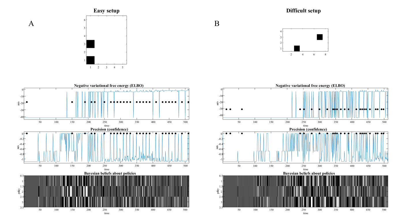<details> <summary>x5.png Details</summary>  ### Visual Description ## [Multi-Panel Technical Figure]: Comparison of Easy vs. Difficult Experimental Setups ### Overview The image is a composite figure containing two main columns, labeled **A** and **B**, which compare results from an "Easy setup" and a "Difficult setup," respectively. Each column contains four plots: a top scatter plot and three time-series plots below it. The figure appears to present data from a computational or machine learning experiment, likely involving Bayesian inference, active inference, or reinforcement learning, tracking metrics like variational free energy (ELBO), precision (confidence), and policy beliefs over time. ### Components/Axes **Top Row (Scatter Plots):** * **Plot A (Left):** Titled **"Easy setup"**. It is a 2D scatter plot with an x-axis ranging from 1 to 5 and a y-axis ranging from 1 to 6. Two black square markers are present: one at approximate coordinates **(1, 1)** and another at **(1, 3)**. * **Plot B (Right):** Titled **"Difficult setup"**. It is a 2D scatter plot with an x-axis ranging from 2 to 8 and a y-axis ranging from 1 to 4. Two black square markers are present: one at approximate coordinates **(3, 1)** and another at **(7, 3)**. **Time-Series Plots (Both Columns A and B share identical structure):** 1. **Top Time-Series:** Titled **"Negative variational free energy (ELBO)"**. * **X-axis:** Label is **"time"**, scale from 0 to 500. * **Y-axis:** Label is **"nats"**, scale from -40 to 0. * **Data:** A continuous blue line plot with overlaid black circular dots at specific time points. 2. **Middle Time-Series:** Titled **"Precision (confidence)"**. * **X-axis:** Label is **"time"**, scale from 0 to 500. * **Y-axis:** Label is **"nats"**, scale from -1 to 0. * **Data:** A continuous blue line plot with overlaid black circular dots at specific time points. 3. **Bottom Time-Series:** Titled **"Bayesian beliefs about policies"**. * **X-axis:** Label is **"time"**, scale from 0 to 500. * **Y-axis:** Label is **"policy"**, scale from 0.5 to 3.5. * **Data:** A grayscale heatmap or raster plot. The intensity (darkness) represents the probability or belief strength for different discrete policies (y-axis) over time (x-axis). Darker shades indicate higher belief. ### Detailed Analysis **A. Easy Setup Time-Series Trends:** * **ELBO:** The blue line starts near -40 nats. Around time=150, it begins to exhibit sharp, frequent upward spikes towards 0 nats, interspersed with returns to lower values. From approximately time=250 onward, the signal oscillates rapidly between high (near 0) and low values, with the black dots appearing predominantly during the high-value phases. * **Precision:** The blue line shows a pattern of frequent, sharp drops from near 0 nats down to -1 nats, especially between time=50-150. After time=150, the drops become more frequent and are often followed by rapid recoveries. The black dots are clustered during periods where the precision is sustained near 0. * **Bayesian Beliefs:** The heatmap shows distinct vertical bands. Initially (time 0-50), belief is concentrated on a single policy (around y=1.5). Over time, belief shifts and becomes distributed across multiple policies (y=1 to 3), with clear, rapid transitions between dominant policies, visualized as sharp changes from light to dark vertical stripes. **B. Difficult Setup Time-Series Trends:** * **ELBO:** Similar initial low value. The first major upward spike occurs later, around time=220. The subsequent oscillations between high and low values appear more erratic and less densely packed than in the Easy setup. The black dots are scattered, with a notable cluster after time=300. * **Precision:** Shows a very sparse pattern of drops to -1 nats before time=100. After time=100, it enters a phase of extremely frequent and deep oscillations between 0 and -1 nats, which continues for the remainder of the timeline. The black dots are sparse early on but become densely clustered after time=300, aligning with the period of intense oscillation. * **Bayesian Beliefs:** The heatmap shows a more gradual and complex evolution of beliefs. There is less clear, sustained dominance of a single policy compared to the Easy setup. The transitions between policy beliefs appear more frequent and noisier, with many policies showing intermediate (gray) levels of belief simultaneously. ### Key Observations 1. **Temporal Onset:** The "Difficult setup" shows a delayed onset of significant activity (spikes in ELBO, drops in Precision) compared to the "Easy setup." 2. **Signal Character:** The "Easy setup" time-series, particularly after time=250, show more regular, high-frequency oscillations. The "Difficult setup" signals appear more chaotic and less periodic. 3. **Dot Alignment:** In both setups, the black dots (likely indicating decision points, observations, or actions) tend to cluster during periods of high ELBO (near 0 nats) and high Precision (near 0 nats). This correlation is more pronounced in the latter half of the timelines. 4. **Policy Belief Dynamics:** The "Easy setup" exhibits clearer, more decisive shifts in policy belief (sharp black/white transitions). The "Difficult setup" shows more ambiguous, distributed beliefs (more gray areas) and faster, less stable switching. ### Interpretation This figure contrasts the performance of an agent or model under two conditions of environmental or task difficulty. * **What the data suggests:** The "Easy setup" allows the system to achieve high ELBO (good model fit/evidence accumulation) and high precision (confidence) more quickly and maintain it with regular, confident updates (dots). Its policy beliefs are decisive. The "Difficult setup" delays this convergence. The system struggles initially, then enters a state of high but unstable confidence (frequent precision drops) and erratic model evidence (ELBO spikes). Its policy beliefs remain uncertain and fluctuate rapidly, suggesting difficulty in identifying a stable, optimal strategy. * **Relationship between elements:** The top scatter plots likely define the experimental conditions (e.g., locations of targets or stimuli in a 2D space). The time-series show the internal state of the agent responding to those conditions. High ELBO and Precision are prerequisites for confident policy selection, as seen by the dot clustering. The Bayesian beliefs plot is the direct output of this inference process. * **Notable anomalies/trends:** The most striking trend is the **phase transition** in both setups around a specific time (≈150 for Easy, ≈220 for Difficult), where the system shifts from a low-activity state to a high-activity, oscillatory state. The "Difficult setup" never achieves the same regularity or stability as the "Easy setup," indicating a fundamental limit in its ability to resolve the more challenging task configuration. The persistent oscillations in Precision in the Difficult case may reflect a system constantly testing and rejecting hypotheses. </details> Figure 5: The emergence of play. Panels $A$ and $B$ show the results of two simulations of $512$ time steps (i.e., about two minutes of simulated time) under two configurations of the Pong set up: an easy setup in panel A and a slightly more difficult setup in panel B, in which the width of the bounding box was increased, and its height decreased (from $5× 6$ to $8× 4$ ). In both panels, the configuration of the game is shown above three plots reporting fluctuations in various measures of belief updating, and accompanying behaviour. The first graph plots the (negative) variational free energy as a function of time (where each time step corresponds roughly to $250$ ms). The black dots mark time points when the ball was hit. It can be seen that during accumulation of the likelihood Dirichlet counts, the ball was missed until time step $150$ . After about a minute, the synthetic agent then starts to emit short rallies of between one and seven consecutive hits. The emergence of game play is accompanied by saltatory increases in negative variational free energy (or evidence lower bound). These increases disappear whenever the agent misses the ball, terminating little rallies. The second graph plots the average of the expected free energy under posterior beliefs about policies. This can be read as the precision of policy beliefs or, more colloquially, the confidence placed in policy selection. This illustrates that confident behaviour emerges during the first minute and is subsequently restricted to moments prior to hitting the ball. Heuristically, this can be read as the agent realising that it can avoid ambiguity by move moving in such a way as to catch the ball. The accompanying posterior (Bayesian) beliefs about policies are shown in image format in the lower plot. This illustrates that precise or confident behaviour entails precise beliefs about what to do next. Panel $B$ shows exactly the same results but for a slightly more difficult game. Here, the ball has more latitude to move horizontally and is returned more quickly, due to the reduced height of the bounding box. In consequence, learning a precise likelihood mapping takes about twice the amount of time. And, even when learned, the rallies are shorter, ranging from one to four, at most. We will use this more difficult set up to look at the effect of inductive planning in the next figure. ### 4.1 Inductive Planning In this section, we repeat the simulations above, but making the game more difficult by increasing the width of the box. This means that to catch the ball, the agent has to anticipate outcomes in the distal future in order to respond with pre-emptive movement of the paddle. Note that this kind of behaviour goes beyond the sort of behaviour predicted under perceptual control theory and related accounts of ball catching [69, 70]. For example, one way to model behaviour in this paradigm would be to move the paddle so that it was always underneath the ball. However, this is not the behaviour that emerges under self-evidencing. In what follows, we will see that avoiding ambiguity is not sufficient for skilled performance of a more difficult game of Pong. However, if we equip the agent with intentions to hit the ball (i.e., as an intended state), it can use inductive planning to pursue a never ending rally, and play the game skilfully. Figure 5 (B) reports performance over about two minutes of simulated time of an abductive agent when increasing the width of the Pong box to $8$ units (and decreasing its height to $4$ units). This simple change precludes sustained rallies; largely because the depth of planning is not sufficient to support pre-emptive moves of the paddle. The equivalent results under inductive planning are shown in Figure 6. Here, active inference under inductive constraints produces intermittent rallies within about a minute of simulated time—and skilled, and fluent play after three minutes. 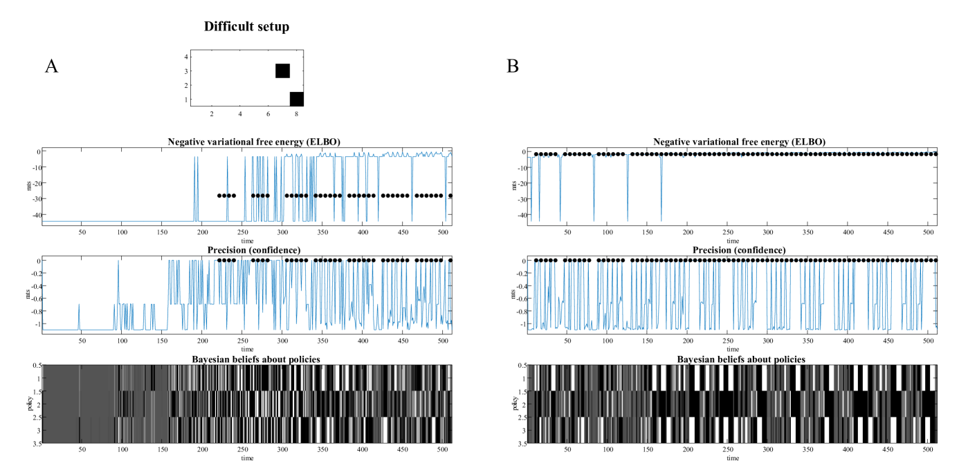<details> <summary>x6.png Details</summary>  ### Visual Description \n ## Scientific Figure: Comparative Analysis of Two Experimental Setups ### Overview The image is a scientific figure titled "Difficult setup," presenting a side-by-side comparison of two experimental conditions or model runs, labeled **A** (left column) and **B** (right column). Each column contains four vertically stacked plots that track different metrics over a common time axis (0 to 500 units). The figure appears to analyze the performance and internal states of a Bayesian or active inference agent navigating a task. ### Components/Axes **Global Structure:** * **Main Title:** "Difficult setup" (centered at the top). * **Column Labels:** "A" (top-left of left column), "B" (top-left of right column). * **Common X-Axis:** All time-series plots share an x-axis labeled "time" with major ticks at 0, 50, 100, 150, 200, 250, 300, 350, 400, 450, 500. **Plot 1 (Top of each column): Small Scatter/Grid Plot** * **Title:** None explicitly, but contextually represents the task environment or state space. * **Y-Axis:** Unlabeled, with numerical ticks at 1, 2, 3, 4. * **X-Axis:** Unlabeled, with numerical ticks at 2, 4, 6, 8. * **Content:** A 2D grid. In both A and B, two black squares are plotted: one at approximately (x=7, y=3) and another at (x=8, y=1). This likely represents target locations or obstacles in a spatial task. **Plot 2: Negative variational free energy (ELBO)** * **Title:** "Negative variational free energy (ELBO)" * **Y-Axis:** Labeled "nats" (a unit of information). Scale ranges from approximately -45 to 0. * **Content:** A blue line plot showing the time series of the Evidence Lower BOund (ELBO), a key quantity in variational inference. Black dots are overlaid on the plot at specific time points. **Plot 3: Precision (confidence)** * **Title:** "Precision (confidence)" * **Y-Axis:** Labeled "nats". Scale ranges from approximately -1.1 to 0. * **Content:** A blue line plot showing the time series of a precision or confidence parameter. Black dots are overlaid, corresponding in time to those in the ELBO plot above. **Plot 4 (Bottom of each column): Bayesian beliefs about policies** * **Title:** "Bayesian beliefs about policies" * **Y-Axis:** Labeled "p(policy)". Scale ranges from 0 to 0.5. * **X-Axis:** Labeled "time". * **Content:** A heatmap (grayscale) where the y-axis represents discrete policies (indexed 1 through 4, based on the tick marks at 0.5, 1.5, 2.5, 3.5). The grayscale intensity at each (time, policy) coordinate represents the probability assigned to that policy. A color bar is not present, but darker shades likely indicate higher probability. ### Detailed Analysis **Setup A (Left Column):** 1. **ELBO Plot:** The blue line shows high volatility. It starts near -45, exhibits frequent, sharp spikes toward 0, and becomes increasingly noisy after time ~200. Black dots appear in distinct clusters: a dense cluster from ~t=220-240, another from ~t=260-280, and then regularly spaced dots from ~t=300 onward. 2. **Precision Plot:** The blue line is also highly volatile, oscillating rapidly between approximately -1.0 and 0. The pattern of black dots mirrors that in the ELBO plot exactly. 3. **Bayesian Beliefs Heatmap:** Shows a complex, shifting pattern of policy probabilities. Initially (t=0-50), policy 1 (top row) has moderate probability (medium gray). Over time, the probability mass shifts dynamically between all four policies, with frequent, sharp transitions. No single policy dominates for an extended period. **Setup B (Right Column):** 1. **ELBO Plot:** The blue line shows a different pattern. It starts near -45, quickly jumps to near 0, and remains relatively stable with minor fluctuations. There are a few isolated, deep downward spikes (e.g., near t=30, 80, 170). Black dots are present almost continuously from the start, forming a near-solid line along the top of the plot. 2. **Precision Plot:** Similar to Setup A's precision plot in volatility, oscillating between -1.0 and 0. The black dots are also nearly continuous. 3. **Bayesian Beliefs Heatmap:** Shows a more stable, structured pattern. From the beginning, policy 2 (second row from top) is assigned very high probability (black) and remains dominant for long stretches, especially from t=0-100 and t=200-350. There are brief periods where probability shifts to other policies (e.g., policy 3 around t=150-200), but the system consistently returns to a strong belief in policy 2. ### Key Observations * **Dot Correlation:** The black dots in the ELBO and Precision plots are perfectly synchronized in time within each setup. Their density differs dramatically: sparse and clustered in A vs. dense and continuous in B. * **ELBO Stability:** Setup B achieves and maintains a high (near-zero) ELBO value much more consistently than Setup A, which shows persistent volatility. * **Policy Certainty:** The heatmap for Setup B shows long periods of high confidence (dark bands) in a single policy (policy 2). Setup A's heatmap shows constant flux and lower overall confidence (lighter, more varied grays). * **Initial Conditions:** Both setups begin with the same ELBO (~-45) and the same environmental configuration (the two black squares in the top plot). ### Interpretation This figure compares the learning or decision-making dynamics of two agents (or the same agent under two conditions) in a "difficult" task environment. * **What the data suggests:** Setup B represents a successful or convergent run. The agent quickly identifies a high-value policy (policy 2), leading to a stable, high ELBO (good model evidence) and high precision/confidence. The near-continuous black dots may indicate frequent policy execution or evaluation. Setup A represents a struggling or non-convergent run. The agent fails to settle on a stable policy, resulting in volatile ELBO and precision, and constantly shifting beliefs. The clustered dots may represent sporadic attempts to execute a policy when confidence momentarily peaks. * **Relationship between elements:** The ELBO is the objective function being maximized. High, stable ELBO (as in B) correlates with stable, high-confidence policy beliefs. Low, volatile ELBO (as in A) correlates with uncertain, shifting policy beliefs. Precision appears to be a related confidence metric that fluctuates rapidly in both cases, but its sustained high values in B (implied by the continuous dots) support stable policy selection. * **Notable Anomalies/Outliers:** The deep, isolated downward spikes in Setup B's ELBO are notable. They suggest momentary catastrophic drops in model evidence, possibly due to encountering a surprising state or making a poor decision, but the agent recovers quickly. The initial identical conditions followed by divergent paths highlight the potential role of stochasticity or slight initial differences in leading to vastly different outcomes in complex tasks. * **Peircean Investigation:** The evidence (divergent time-series patterns) points to a fundamental difference in the *process* of inference between the two setups. Setup B exhibits signs of *abductive reasoning* settling on a consistent explanatory model (policy). Setup A remains trapped in a cycle of *inductive* updating without achieving a stable abductive conclusion, indicative of a model or environment mismatch. The "difficult setup" title is validated by the struggle evident in column A. </details> Figure 6: Inductive planning. This figure follows the same format as Figure 5, reporting the emergence of pong-playing behaviour under the more difficult set up described in the previous figure. However, here, we included inductive planning in the belief updating by specifying the agent’s intentions in terms of priors over particular latent states; namely, states in which the agent hit the ball. In realising these intentions, the agent quickly learns a sufficiently precise likelihood mapping, evincing rallies of between four and six. after about a minute (of simulated time). This is shown in panel A. Panel B, shows the performance during the subsequent two minutes. By about three minutes, the agent has a precise grip on its world and realises its intentions fluently. From a dynamical systems perspective, this can be read as the emergence of generalised synchrony—or synchronisation of chaos—as the joint system converges onto a synchronisation manifold: a manifold that contains the states the agent intends to visit. In this example, we simply specified the intended states as those states corresponding to ball hits. This would be like instructing a child by telling her what is (i.e., which states are) expected of her. She can then work out how to realise those states by using inductive planning and selecting the most likely actions at each moment. Notice that there is no sense in which this could be construed as reinforcement learning: no reward or cost is being optimised, rather the behaviour is driven purely by the minimisation of uncertainty. A better metaphor would be instantiating some intentional set by instilling intentions or prior beliefs about characteristic states that should be realised. From the perspective of the free energy principle, priors over intended states can be cast as specifying a non-equilibrium steady-state with a (pullback) attractor that contains intended or characteristic states. From a dynamical systems perspective, this is equivalent to specifying unstable fixed points that characterise stable heteroclinic orbits [71, 72], which have been discussed in terms of sequential behaviour [73]. Intuitively, this means the agent has found a free energy minimum that is characterised by generalised synchrony between the neuronal network and the process generating sensory inputs. Given that this synchronisation was never seen in the in vitro experiments, one might argue that the in vitro behaviour was sentient but not intentional. In the remaining sections, we briefly showcase inductive planning in two other paradigms to illustrate the interaction between constraints—encoded by prior preferences over outcomes—and prior intentions, encoded by priors over latent states. ## 5 Navigation as Inductive Planning In this section, we revisit a simple navigation problem addressed many times in the literature; e.g., [74, 75] and in demonstrations of active inference: e.g., [8, 76]. Here, the problem is to learn the structure of a two-dimensional maze and then navigate to a target location based upon what has been learned. This features the dual problem of learning a world or generative model and then using what has been learned for deep planning and navigation. In detail, we constructed a simple maze—shown in Figure 7 —for an agent who has a myopic view of the world; namely, one output modality that reported whether the agent was sitting on an allowable location (white square) in the maze or a disallowed location (black square), which, a priori, it found surprising (e.g., experiencing a foot shock). A simple generative model was supplied to the agent in the form of a single factor encoding each location or way-point, equipped with five paths. These were controllable paths that moved the agent up or down, or right or left (or staying still). The likelihood mapping was, as in the previous simulation, initialised to small uniform Dirichlet counts. This means the agent has no idea about the structure of its world but simply knew that a latent state could change in one of five ways. Learning this kind of environment is straightforward under active inference, due to the novelty or expected information gain about parameters (see Equation 2). This means the agent chooses actions that resolve the greatest amount of uncertainty in the likelihood mapping from each latent state to outcomes. This ensures a Bayes optimal exploration of state space. Figure 7 A shows that the agent pursues a path which covers all locations in an efficient fashion: i.e., not revisiting experienced states or locations until it has explored every location. The trajectory shown in Figure 7 A corresponds to $256$ time steps. After this exposure, the agent has learned a likelihood model that is sufficient to support inductive planning. Figures 7 B and C shows the results of this inductive navigation, reaching a distal target (red dot) from a starting location, while avoiding surprises or black squares in the maze. The two routes chosen are under imprecise and precise prior preferences for avoiding black squares (i.e., a log odds ratio—encoded by $c$ —of one and four, respectively). Note that the path under precise preferences is about $20$ steps, speaking to the depth of induction (here, $32$ time steps, as in Figure 3). This example highlights an interesting aspect of inductive planning as defined here: namely, the learned constraints on foraging act as constraints on intentional behaviour. These constraints enter the allowable transitions, so that the paths that are induced respect the constraints due to prior preferences that can be inferred after—and only after—learning the likelihood mapping. In short, this example shows how it is possible to reach intended endpoints, under constraints on the way one gets there. In the final section, we use the same scheme to illustrate the efficiency of inductive planning in high dimensional problem spaces. 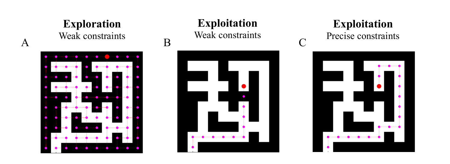<details> <summary>x7.png Details</summary>  ### Visual Description ## Diagram: Exploration vs. Exploitation Strategies in a Maze Environment ### Overview The image displays three side-by-side diagrams (labeled A, B, and C) illustrating different agent strategies within an identical maze environment. Each diagram shows a black square maze with white pathways. A path traced by magenta dots represents the agent's trajectory, and a single red dot marks the agent's current or final position. The diagrams compare "Exploration" and "Exploitation" under different constraint conditions. ### Components/Axes * **Layout:** Three square maze diagrams arranged horizontally. * **Labels (Top):** * **A:** "Exploration" (bold), "Weak constraints" (regular font) * **B:** "Exploitation" (bold), "Weak constraints" (regular font) * **C:** "Exploitation" (bold), "Precise constraints" (regular font) * **Labels (Left):** The letters "A", "B", and "C" are positioned to the left of their respective mazes. * **Visual Elements:** * **Maze Structure:** A fixed, complex maze layout with walls (black) and passages (white). The structure is identical in all three diagrams. * **Path (Magenta Dots):** A series of connected magenta dots traces the route taken by the agent through the white passages. * **Agent (Red Dot):** A single, larger red dot indicates the agent's location. * **Legend (Implied):** The color coding is consistent: Magenta = Agent's path/history; Red = Agent's current position. ### Detailed Analysis **Diagram A: Exploration (Weak constraints)** * **Path Description:** The magenta path is extensive and dense, covering nearly all accessible white passages in the maze. It forms a complex, branching network that reaches most dead ends and corridors. * **Agent Position:** The red dot is located in the upper-right quadrant of the maze, at the end of a long, winding path from the bottom-left starting area. * **Trend:** The visual trend is one of comprehensive coverage, indicating the agent has visited a large proportion of the state space. **Diagram B: Exploitation (Weak constraints)** * **Path Description:** The magenta path is significantly shorter and more direct than in A. It follows a specific route from the bottom-left start, moving right, then up, then right again into a central corridor. It does not explore side passages. * **Agent Position:** The red dot is located in the central-right area of the maze, at the terminus of this direct path. * **Trend:** The visual trend is goal-directed and efficient, focusing on a single, seemingly optimal route without deviation. **Diagram C: Exploitation (Precise constraints)** * **Path Description:** The magenta path is very similar to Diagram B, following the same general efficient route. However, there is a subtle but critical difference: the path makes a small, precise detour or loop in the upper-right section before returning to the main corridor. This suggests adherence to a more specific or refined rule set. * **Agent Position:** The red dot is located in the same central-right corridor as in B, but its position relative to the path's end is slightly different due to the detour. * **Trend:** The trend is still efficient and goal-directed, but with an added layer of precision or adherence to a stricter policy, resulting in a minor variation in the path. ### Key Observations 1. **Path Density Gradient:** There is a clear visual gradient in path density from A (very high) to B and C (low). This directly illustrates the core trade-off: exploration consumes more resources (time, steps) to gather information, while exploitation uses gathered information to act efficiently. 2. **Identical Environment, Different Behavior:** The maze structure is constant, proving that the differences in agent behavior are due solely to the chosen strategy (Exploration vs. Exploitation) and the nature of the constraints (Weak vs. Precise). 3. **Constraint Impact:** Comparing B and C shows that "Precise constraints" lead to a more nuanced path than "Weak constraints," even under the same high-level strategy of exploitation. The precise constraints likely enforce a more specific policy, preventing the minor inefficiencies or variations seen in the weak constraint version. 4. **Spatial Grounding:** In all diagrams, the agent starts in the bottom-left corner. The exploration path (A) fills the space from this origin. The exploitation paths (B, C) show a clear, linear progression from origin to a goal region in the center-right. ### Interpretation This diagram is a pedagogical visualization of fundamental concepts in reinforcement learning and decision theory. * **Exploration vs. Exploitation:** Diagram A represents an agent prioritizing **exploration**—gathering maximum information about the environment's structure, even at the cost of immediate efficiency. This is crucial in unknown environments to build an accurate model. Diagrams B and C represent **exploitation**—using existing knowledge to maximize reward or reach a goal quickly. The trade-off is clear: exploration builds a better long-term model but is slow; exploitation is fast but risks being suboptimal if the model is incomplete. * **Role of Constraints:** "Weak constraints" (A & B) likely refer to a loose policy or objective function, allowing for more randomness or broader goals (e.g., "visit many states" or "reach the general goal area"). "Precise constraints" (C) imply a stricter, more defined policy (e.g., "follow this exact sequence of actions" or "adhere to this specific safety rule"), which refines the agent's behavior even within an exploitation framework. * **Underlying Message:** The image argues that the optimal strategy is context-dependent. In a completely unknown maze, starting with behavior like A is necessary. Once a good map is built (knowledge from A), switching to behavior like B or C is efficient. The difference between B and C highlights how the specificity of the learned policy or external rules fine-tunes exploitative behavior. The diagrams effectively translate abstract algorithmic concepts into an intuitive spatial narrative. </details> Figure 7: Navigation by induction. A: this panel reports the exploration of an agent that is building its likelihood mapping by exploring all the novel locations in a maze. Initially, the agent does not know where it can go; in the sense that it can only see its current location, which can be black or white. Therefore, every unvisited location furnishes some novelty; i.e., expected information gain (about likelihood parameters). This compels the agent to explore all locations efficiently and uniformly with an effective inhibition of return, until it has become familiar with this particular maze layout. After learning, the agent was given some intentions in terms of a specific location it believed, a priori, it would visit. Panels B and C show the results of planning under mild and precise preferences for being on white squares. In panel B, the agent takes a short cut to the target location (red dot), which involves a transgression of one black square. This means that the cost of being on black squares is not sufficiently precise to have constrained the transitions used in inductive planning. However, because the agent is still trying to minimise expected cost (encoded by preferences for white squares) it navigates fairly gracefully until it encounters a barrier. In contrast, panel C shows the same agent with precise costs, which preclude transitions to black squares during inductive planning. This agent can swiftly induce the requisite path to the target location, without transgressing constraints on outcomes. ## 6 Inductive Problem Solving This section considers a canonical problem solving task; namely, the Tower of Hanoi [77]. In this problem, one has to rearrange a number of balls over a number of towers to reach a target arrangement from any given initial arrangement: see Figure 8. The problem can be made easier or more difficult by manipulating the number of intervening rearrangements between the initial and target (intended) configurations. We have previously shown that this problem can be learned from scratch using structure learning [78]. Here, we consider problem-solving with and without inductive planning, after learning the likelihood model and allowable state transitions. As above, implementing inductive planning simply means equipping the agent with prior beliefs about a final (intended) state and then letting it rearrange the balls until those intended states are realised. To solve this problem using active inference, one usually supplies constraints in terms of prior preferences that are mildly aversive for all but the target arrangement. This means the agent will rearrange the balls, in a state of mild surprise until the preferred arrangement is found—and the agent rests in a low free energy state. Because constraints are only in outcome space, there are certain arrangements that are less surprising because they are similar to the target configuration (as defined in outcome space). This enables the agent to solve fairly deep problems, even with a limited depth of planning (here, one-step-ahead planning). However, problems requiring more than four or five moves usually confound this kind of planning as inference. In contrast, if the intended target is specified in state space, then it will invoke inductive planning and, in principle, solve difficult problems, even with a limited depth of planning. 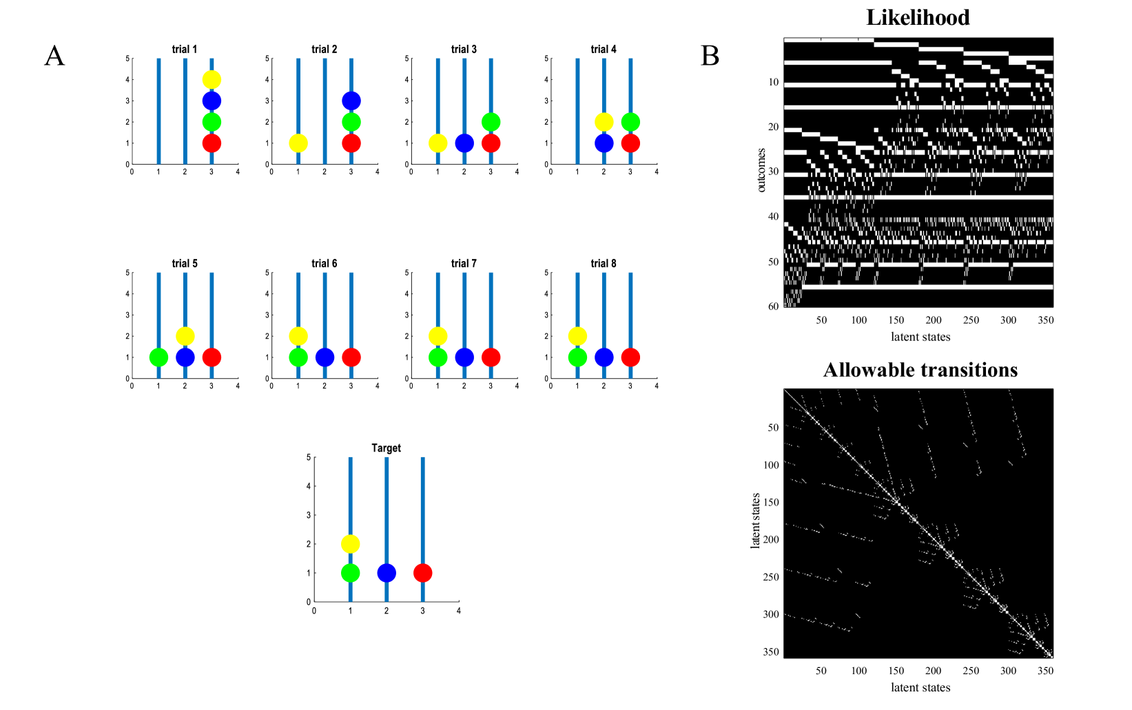<details> <summary>x8.png Details</summary>  ### Visual Description ## Multi-Panel Technical Figure: Experimental Trials and State Transition Matrices ### Overview The image is a composite figure containing two main panels, labeled **A** and **B**. Panel A displays a series of 8 experimental trials and a final "Target" configuration, visualized as colored dots on vertical bars. Panel B contains two large heatmap-style matrices titled "Likelihood" and "Allowable transitions," which appear to represent relationships between "latent states" and "outcomes." The overall figure likely illustrates a process of learning or optimization, where trials in Panel A attempt to match a target configuration, and Panel B visualizes the underlying model's structure. ### Components/Axes **Panel A (Left Side):** * **Structure:** A 3x3 grid of small bar charts (with the bottom-right position empty). The charts are labeled: `trial 1`, `trial 2`, `trial 3`, `trial 4` (top row); `trial 5`, `trial 6`, `trial 7`, `trial 8` (middle row); `Target` (bottom row, centered). * **Axes (for each chart):** * **X-axis:** Unlabeled, with numerical markers at `0`, `1`, `2`, `3`, `4`. * **Y-axis:** Unlabeled, with numerical markers from `0` to `5` in increments of 1. * **Data Elements:** Each chart contains three vertical blue bars positioned at x=1, x=2, and x=3. Colored circles (dots) are placed on these bars at specific y-values. * **Color Key (Implicit):** Four distinct colors are used for the dots: **Yellow**, **Blue**, **Green**, **Red**. Their meaning is not explicitly stated in a legend but is consistent across all trials. **Panel B (Right Side):** * **Top Matrix: "Likelihood"** * **X-axis:** Labeled `latent states`, with numerical markers at `50`, `100`, `150`, `200`, `250`, `300`, `350`. * **Y-axis:** Labeled `outcomes`, with numerical markers at `10`, `20`, `30`, `40`, `50`, `60`. * **Content:** A black-and-white (binary) matrix. White pixels represent a value of 1 (or "high likelihood"), and black pixels represent 0 (or "low likelihood"). * **Bottom Matrix: "Allowable transitions"** * **X-axis:** Labeled `latent states`, with numerical markers at `50`, `100`, `150`, `200`, `250`, `300`, `350`. * **Y-axis:** Labeled `latent states`, with numerical markers at `50`, `100`, `150`, `200`, `250`, `300`, `350`. * **Content:** A black-and-white (binary) matrix. White pixels indicate a permissible transition from the state on the x-axis to the state on the y-axis. ### Detailed Analysis **Panel A: Trial Configurations** The position of the colored dots changes across trials, suggesting a sequential adjustment process. The "Target" chart defines the goal state. * **Target Configuration:** * **Bar at x=1:** Green dot at y=1, Yellow dot at y=2. * **Bar at x=2:** Blue dot at y=1. * **Bar at x=3:** Red dot at y=1. * **Trial Progression (Approximate Y-values):** * **trial 1:** (x=3) Red=1, Green=2, Blue=3, Yellow=4. All dots are stacked on the rightmost bar. * **trial 2:** (x=1) Yellow=1. (x=3) Red=1, Green=2, Blue=3. Yellow dot has moved to the leftmost bar. * **trial 3:** (x=1) Yellow=1. (x=2) Blue=1. (x=3) Red=1, Green=2. Blue dot has moved to the center bar. * **trial 4:** (x=2) Blue=1, Yellow=2. (x=3) Red=1, Green=2. Yellow dot moves up on the center bar. * **trial 5:** (x=1) Green=1. (x=2) Blue=1, Yellow=2. (x=3) Red=1. Green dot moves to the leftmost bar. * **trial 6:** (x=1) Green=1, Yellow=2. (x=2) Blue=1. (x=3) Red=1. Yellow dot moves to the leftmost bar. * **trial 7:** (x=1) Green=1, Yellow=2. (x=2) Blue=1. (x=3) Red=1. *Identical to trial 6.* * **trial 8:** (x=1) Green=1, Yellow=2. (x=2) Blue=1. (x=3) Red=1. *Identical to trial 6 and 7.* **Trend Verification:** The sequence shows a clear convergence. Dots start stacked on one bar (trial 1) and are progressively distributed across the three bars. By trial 6, the configuration matches the "Target" exactly, and trials 7 and 8 show no further change, indicating the goal has been achieved and stabilized. **Panel B: State Matrices** * **"Likelihood" Matrix:** This matrix shows a highly structured, non-random pattern. Key features include: * **Horizontal Bands:** Several solid or densely packed white horizontal lines (e.g., near y=5, y=10, y=15, y=25, y=35, y=45, y=55). This indicates that certain outcomes (y-values) are associated with a wide range of latent states. * **Diagonal/Block Structure:** There is a prominent block-diagonal or staircase pattern, particularly visible in the upper half (y=0 to y=30). This suggests clusters of latent states are strongly associated with specific, sequential outcomes. * **Sparse Regions:** The lower half (y=30 to y=60) is more sparse and noisy, with fewer large, coherent white blocks. * **"Allowable transitions" Matrix:** This matrix is predominantly black with white pixels forming a specific pattern. * **Strong Main Diagonal:** A clear, continuous white line runs from the top-left (0,0) to the bottom-right (350,350). This indicates that the most common or allowable transition is from a state to itself (self-transitions). * **Off-Diagonal Points:** Scattered white pixels appear near the main diagonal, forming a thin band. This suggests that transitions are primarily allowed between a state and its immediate neighbors (e.g., state `n` can transition to `n-1`, `n`, or `n+1`). * **Structured Off-Diagonal Clusters:** There are also distinct, sparse clusters of white points further from the diagonal (e.g., around (150, 50) and (250, 150)). These represent specific, non-adjacent state transitions that are permitted by the model. ### Key Observations 1. **Convergence in Panel A:** The system reaches its target configuration by trial 6 and remains stable thereafter. The movement of dots appears methodical, one or two per trial. 2. **Color Consistency:** The four colors (Yellow, Blue, Green, Red) are used consistently across all trials and the target, implying they represent four distinct entities or parameters being positioned. 3. **Matrix Structure in Panel B:** Neither heatmap is random. The "Likelihood" matrix has clear horizontal and block-diagonal features, while the "Allowable transitions" matrix is dominated by a diagonal band, indicating a strong locality constraint in the state space. 4. **Scale Discrepancy:** The "latent states" axis in Panel B (0-350) is much larger than the simple 3-bar system in Panel A, suggesting Panel B describes a more complex, high-dimensional underlying model. ### Interpretation This figure likely comes from a study on **structured learning, planning, or state-space modeling**. * **Panel A** demonstrates a **successful optimization or learning process**. The agent (or algorithm) starts with a poor, stacked configuration and iteratively adjusts the positions of four colored components across three locations to match a predefined target. The stability from trial 6 onward confirms the solution is found and robust. * **Panel B** reveals the **internal structure of the model** governing this process. The "Allowable transitions" matrix defines the "rules of movement" in the latent state space—primarily local moves with a few specific long-range jumps allowed. The "Likelihood" matrix maps these latent states to observable outcomes, showing that outcomes are not independent but are generated by structured, clustered states. The horizontal bands in the Likelihood matrix might represent "default" or highly probable outcomes across many states. * **Connection:** The simple, discrete task in Panel A is likely a **visualization or test case** for an algorithm that operates within the complex, high-dimensional state space characterized by the matrices in Panel B. The algorithm's success in Panel A validates its ability to navigate the allowable transitions and find a state configuration with high likelihood for the target outcome. The figure as a whole argues for the effectiveness of a model that respects structured, local transitions in its latent space to solve concrete positioning tasks. </details> Figure 8: Inductive planning and the Tower of Hanoi. Panel A illustrates the particular game used to illustrate inductive planning. Here, there are four balls on three towers. The problem is to rearrange the initial configuration (on the upper left) to match the target configuration (lowest arrangement). In this example, it takes five moves. Actions correspond to moving a ball from one pillar to another. The generative model that supports this kind of problem solving is shown in terms of the requisite likelihood and transition mappings in panel B. The likelihood tensors have been stacked on top of each other (and unfolded) to illustrate the mapping between the $360$ latent states and the ( $4× 3× 5$ =) $60$ outcomes. The accompanying transition parameters are shown in terms of allowable transitions among latent states (as in Figure 3). This generative model can be learned from scratch by presenting each arrangement—and then each rearrangement—of the balls to accumulate the appropriate Dirichlet parameters. Of interest here, is the use of the ensuing parameters or knowledge to solve problems that require deep planning. This problem is straightforward to solve using inductive planning; namely, working backwards from the target state using the protocol described in Figure 3. The ensuing performance is shown in the next figure. Figure 9 shows the performance of two agents on $100$ problems, given $12$ moves for each problem. The first (abductive) agent was equipped only with constraints in outcome space; i.e., prior preferences that led to the target solution, provided that solution was reasonably close in outcome space. This agent failed to solve problems with five or more moves. In contrast, when specifying intentions in the form of the intended (target) state or arrangement, the second (inductive) agent was able to solve problems of eight moves or more almost instantaneously, without fail. In these examples, the output space was a collection of $(4× 3=)12$ outcome modalities—one for each location or pixel—with five levels (four coloured balls or an empty outcome). The state space encompassed 360 arrangements, producing large ( $360× 360× 5$ ) transition tensors. However, reducing these to logical matrices—used in inductive planning—means one can effectively plan deep into the future (here, $64$ moves) within milliseconds, using a one-step-ahead, active inference scheme. 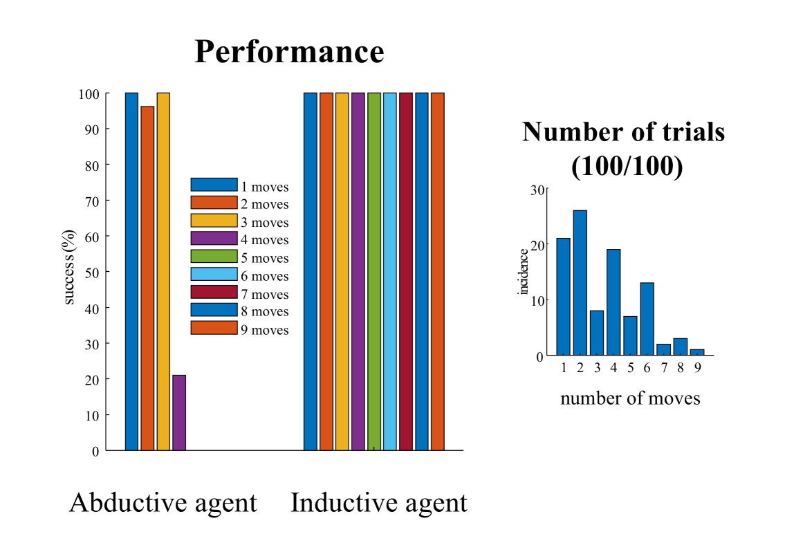<details> <summary>x9.png Details</summary>  ### Visual Description ## Bar Chart and Histogram: Performance and Trial Distribution ### Overview The image contains two distinct charts presented side-by-side. The primary chart on the left is a grouped bar chart comparing the success rates of two agents ("Abductive agent" and "Inductive agent") across tasks requiring different numbers of moves (1 through 9). The secondary chart on the right is a histogram showing the distribution (incidence) of the number of moves required across 100 trials. ### Components/Axes **Left Chart (Grouped Bar Chart):** * **Title:** "Performance" * **Y-axis:** Label is "success(%)". Scale runs from 0 to 100 in increments of 10. * **X-axis:** Two categorical groups: "Abductive agent" (left group) and "Inductive agent" (right group). * **Legend:** Positioned centrally between the two agent groups. It maps colors to the "number of moves" required for a task: * Blue: 1 move * Orange: 2 moves * Yellow: 3 moves * Purple: 4 moves * Green: 5 moves * Light Blue: 6 moves * Dark Red: 7 moves * Dark Blue: 8 moves * Dark Orange: 9 moves **Right Chart (Histogram):** * **Title:** "Number of trials (100/100)" * **Y-axis:** Label is "incidence". Scale runs from 0 to 30 in increments of 10. * **X-axis:** Label is "number of moves". Categories are discrete integers from 1 to 9. * **Data Series:** A single series of blue bars representing the count of trials for each move number. ### Detailed Analysis **Left Chart - Success Rates by Agent and Move Count:** * **Abductive Agent:** * **Trend:** Success is very high for low move counts but drops dramatically for higher move counts. * **Data Points (Approximate):** * 1 move (Blue): 100% * 2 moves (Orange): ~96% * 3 moves (Yellow): 100% * 4 moves (Purple): ~21% * 5 moves (Green): 0% (bar not visible) * 6 moves (Light Blue): 0% (bar not visible) * 7 moves (Dark Red): 0% (bar not visible) * 8 moves (Dark Blue): 0% (bar not visible) * 9 moves (Dark Orange): 0% (bar not visible) * **Inductive Agent:** * **Trend:** Perfect success across all move counts. * **Data Points:** All bars (1 through 9 moves) reach the 100% line. **Right Chart - Distribution of Moves Required:** * **Trend:** The distribution is right-skewed. The most common number of moves required is 2, with incidence decreasing as the number of moves increases. * **Data Points (Approximate Incidence):** * 1 move: 21 * 2 moves: 26 * 3 moves: 8 * 4 moves: 19 * 5 moves: 7 * 6 moves: 13 * 7 moves: 2 * 8 moves: 3 * 9 moves: 1 ### Key Observations 1. **Performance Disparity:** There is a stark contrast between the two agents. The Inductive agent achieves 100% success regardless of task complexity (1-9 moves), while the Abductive agent's performance collapses for tasks requiring 4 or more moves. 2. **Abductive Agent's Threshold:** The Abductive agent shows a clear performance cliff between 3 moves (100% success) and 4 moves (~21% success). 3. **Trial Distribution:** The histogram shows that the evaluation was not uniform across move counts. Tasks requiring 2 moves were most common (26 trials), while tasks requiring 7, 8, or 9 moves were rare (2-3 trials each). 4. **Chart Title Context:** The histogram's title "(100/100)" confirms that the data represents the full set of 100 trials. ### Interpretation This visualization strongly suggests a fundamental difference in capability or strategy between the two agents. The **Inductive agent** demonstrates robust, generalizable problem-solving, maintaining perfect performance as task complexity increases. The **Abductive agent**, however, appears to have a limited operational range, functioning well only for simple tasks (≤3 moves) and failing catastrophically on more complex ones. The histogram provides crucial context for interpreting the left chart. The high success rates for the Abductive agent on 1, 2, and 3-move tasks are based on a substantial number of trials (21, 26, and 8 respectively). Conversely, its 0% success on 7, 8, and 9-move tasks is based on very few trials (2, 3, and 1), which, while still indicative of failure, comes with higher statistical uncertainty. The perfect performance of the Inductive agent is validated across the entire, unevenly distributed trial set. The data implies that for the evaluated problem domain, an inductive reasoning approach is vastly more reliable and scalable than an abductive one. The abductive method may be suitable only for very low-complexity scenarios. </details> Figure 9: Tower of Hanoi Performance. This figure reports the performance of a generative model that has learned the Tower of Hanoi problem in terms of transitions among different arrangements of balls. We presented the agent with $100$ trials with different targets of greater and lesser difficulty (i.e., with varying numbers of moves from the initial and target arrangements). We presented exactly the same problems to agents with and without inductive planning. The right panel shows the incidence of trials in terms of the numbers of moves required until completion. The agent with inductive planning was able to solve $100\$ of trials successfully. In contrast, the agent that did not use inductive planning was only able to complete problems of four moves or less. This is still impressive because both the abductive and inductive agents only looked one step ahead. In other words, even though the abductive agent could only evaluate the quality of its next move, it was still able to work towards the final solution. This is possible because the prior preferences for the target outcomes mean that certain outcomes are closer to the preferred outcomes than others. The 100 trials reported in this figure take less than 10 seconds to simulate. ## 7 Discussion This paper has introduced a particular instance of backwards induction to active inference, as well as a more formal characterisation of sentient and intentional behaviour. Induction in this setting appeals to a simple kind of backwards induction via logical operators, which is used to furnish constraints on the expected free energy, and hence, actions. Actions are then selected in the usual way; namely, actions that maximise expected information gain and value—where value is scored by log prior preferences over outcomes. The use of inductive priors lends planning a deep reach into the future that rests upon specifying final or intended endpoints. In turn, this differentiates sentient from intentional behaviour. To the extent that one can describe Bayesian beliefs—about the ultimate consequences of plans—as intentions, one could describe the behaviour illustrated above as intentional with a well-defined purpose or goal. Inductive planning, as described here, can also be read as importing logical or symbolic (i.e. deductive) reasoning into a probabilistic (i.e., inductive, in the sense of inductive programming) framework. This speaks to symbolic approaches to problem solving and planning—e.g., [79, 80, 81] —and a move towards the network tensor computations found in quantum computing: e.g., [82, 83]. However, in so doing, one has to assume precise priors over state transitions and intended states. In other words, this kind of inductive planning is only apt when one has precisely stated goals and knowledge about state transitions. Is this a reasonable assumption for active inference? It could be argued that it is reasonable in the sense that: (i) goal-states or intended states are stipulatively precise (one cannot formulate an intention to act without specifying the intended outcome with a certain degree of precision) and (ii) the objective functions that underwrite self-evidencing lead to precise likelihood and transition mappings. In other words, to minimise expected free energy—via learning—just is to maximise the mutual information between latent states and their outcomes, and between successive latent states. To conclude, inductive planning differs from previous approaches proposed in both the reinforcement learning and active inference literature, due to the presence of intended goals defined in latent state space. In both model free and model based reinforcement learning, goals are defined via a reward function. In alternative but similar approaches, such as active inference, rewards are passed to the agent as privileged (usually precise but sparse) observations [41, 84]. This influences the behaviour of the agent, which learns to design and select policies that maximise expected future reward either via model-free approaches, which assign values to state-action pairs, or via model-based approaches, which select actions after simulating possible futures. Defining preferences directly in the state space, however, induces a different kind of behaviour: the fast and frugal computation involved in inductive planning is now apt to capture the efficiency of human-like decision-making, where indefinitely many possible paths, inconsistent with intended states, are ruled out a priori —hence combining the ability of agents to seek long-term goals, with the efficiency of short-term planning. ## 8 Conclusion The aim of this paper was to characterise the self-organisation of adaptive behaviour through the lens of the free energy principle, i.e., as self-evidencing. We did this by first discussing the definitions of reactive and sentient behaviour in active inference, where the latter describes the behaviour of agents that are aware of the consequences of their actions. We then introduced a formal account of intentional behaviour, Specified by intended endpoints or goals, defined in state space rather than outcome space, as in abductive forms of active inference. We then investigate these forms of (reactive, sentient, and intentional) behaviour using simulations. First, we simulate the aforementioned in vitro experiments, in which neuronal cultures spontaneously learn to play Pong, by implementing nested, free energy minimising processes. We used these simulations to Illustrate the ensuing behaviour—leveraging the distinction between merely reactive, sentient, and intentional behaviour. The requisite inductive planning was then further illustrated using simple machine learning benchmarks (navigation in a grid world and the Tower of Hanoi problem), that showed how quickly and efficiently adaptive behaviour emerges under inductive constraints on active inference. ## Disclosure statement The authors have no disclosures or conflict of interest. ## Acknowledgements KF is supported by funding for the Wellcome Centre for Human Neuroimaging (Ref: 205103/Z/16/Z), a Canada-UK Artificial Intelligence Initiative (Ref: ES/T01279X/1) and the European Union’s Horizon 2020 Framework Programme for Research and Innovation under the Specific Grant Agreement No. 945539 (Human Brain Project SGA3). AR is funded by the Australian Research Council (Ref: DP200100757) and the Australian National Health and Medical Research Council (Investigator Grant Ref: 1194910). ## References - [1] B.J. Kagan et al. “In vitro neurons learn and exhibit sentience when embodied in a simulated game-world” In Neuron, 2022 - [2] Chris Fields, James F Glazebrook and Michael Levin “Minimal physicalism as a scale-free substrate for cognition and consciousness” In Neuroscience of Consciousness 2021, 2021, pp. niab013 - [3] M. Levin “The Computational Boundary of a "Self": Developmental Bioelectricity Drives Multicellularity and Scale-Free Cognition” In Frontiers in Psychology 10, 2019, pp. 2688 - [4] S. Manicka and M. Levin “Modeling somatic computation with non-neural bioelectric networks” Scientific Reports 9, 18612, 2019 - [5] Atsushi Masumori et al. “Emergence of sense-making behavior by the Stimulus Avoidance Principle: Experiments on a robot behavior controlled by cultured neuronal cells” In Artificial Life Conference Proceedings, 2015, pp. 373–380 MIT Press One Rogers Street, Cambridge, MA 02142-1209, USA journals-info … - [6] T. Isomura and K. Friston “In vitro neural networks minimise variational free energy” In Scientific Reports 8, 2018, pp. 16926 - [7] T. Isomura, K. Kotani, Y. Jimbo and K.J. Friston “Experimental validation of the free-energy principle with in vitro neural networks” In Nature Communications 14, 2023, pp. 4547 - [8] K. Friston et al. “Sophisticated inference” In Neural Computation 33, 2021, pp. 713–763 - [9] E.R. Palacios, T. Isomura, T. Parr and K. Friston “The emergence of synchrony in networks of mutually inferring neurons” In Scientific Reports 9, 2019, pp. 6412 - [10] J. Winn and C.M. Bishop “Variational message passing” In Journal of Machine Learning Research 6, 2005, pp. 661–694 - [11] Jakob Hohwy “The self-evidencing brain” In Noûs 50.2 Wiley Online Library, 2016, pp. 259–285 - [12] V. Mnih et al. “Human-level control through deep reinforcement learning” In Nature 518, 2015, pp. 529–533 - [13] J. Schrittwieser et al. “Mastering Atari, Go, Chess and Shogi by Planning with a Learned Model” arXiv:1911.08265, 2019 - [14] Fuat Balci “A response to claims of emergent intelligence and sentience in a dish” In Neuron 111, 2023, pp. 604–605 - [15] Hagai Attias “Planning by probabilistic inference” In International workshop on artificial intelligence and statistics, 2003, pp. 9–16 PMLR - [16] Matthew Botvinick and Marc Toussaint “Planning as inference” In Trends in cognitive sciences 16.10 Elsevier, 2012, pp. 485–488 - [17] Sander G Van Dijk and Daniel Polani “Informational constraints-driven organization in goal-directed behavior” In Advances in Complex Systems 16.02n03 World Scientific, 2013, pp. 1350016 - [18] Lancelot Da Costa et al. “Active inference on discrete state-spaces: A synthesis” In Journal of Mathematical Psychology 99, 2020, pp. 102447 - [19] Maxwell JD Ramstead et al. “On Bayesian mechanics: a physics of and by beliefs” In Interface Focus 13.3 The Royal Society, 2023, pp. 20220029 - [20] K. Friston et al. “The free energy principle made simpler but not too simple” In Physics Reports 1024, 2023, pp. 1–29 - [21] K. Friston et al. “Path integrals, particular kinds, and strange things” arXiv:2210.12761, 2022 - [22] Colin F Camerer “Progress in behavioral game theory” In Journal of Economic Perspectives 11, 1997, pp. 167–188 - [23] C. Hure, H. Pham and X. Warin “Deep Backward Schemes for High-Dimensional Nonlinear Pdes” In Mathematics of Computation 89, 2020, pp. 1547–1579 - [24] Richard Bellman “On the Theory of Dynamic Programming” In Proc Natl Acad Sci U S A 38, 1952, pp. 716–719 - [25] Lancelot Da Costa et al. “The relationship between dynamic programming and active inference: the discrete, finite-horizon case” In arXiv preprint arXiv:2009.08111, 2020 - [26] R.S. Sutton, D. Precup and S. Singh “Between MDPs and semi-MDPs: A framework for temporal abstraction in reinforcement learning” In Artificial Intelligence 112, 1999, pp. 181–211 - [27] Aswin Paul, Noor Sajid, Lancelot Da Costa and Adeel Razi “On efficient computation in active inference” In arXiv preprint arXiv:2307.00504, 2023 - [28] G.H. Harman “The inference to the best explanation” In Philosophical Review 74, 1965, pp. 88–95 - [29] A.K. Seth “Inference to the Best Prediction” In Open MIND Frankfurt am Main: MIND Group, 2015 - [30] R.A. Howard “Dynamic Programming and Markov Processes” Cambridge, MA: MIT Press, 1960 - [31] M.J.D. Ramstead et al. “On Bayesian Mechanics: A Physics of and by Beliefs” arXiv:2205.11543, 2022 - [32] Andy Clark, Karl Friston and Sam Wilkinson “Bayesing Qualia: Consciousness as Inference, Not Raw Datum” In Journal of Consciousness Studies 26, 2019, pp. 19–33 - [33] L. Sandved-Smith et al. “Towards a computational phenomenology of mental action: modelling meta-awareness and attentional control with deep parametric active inference” In Neuroscience of Consciousness 2021, 2021, pp. niab018 - [34] Ryan Smith, Maxwell J.D. Ramstead and Alex Kiefer “Active Inference Models Do Not Contradict Folk Psychology” In Synthese 200.2 Springer Verlag, 2022, pp. 1–37 DOI: 10.1007/s11229-022-03480-w - [35] Matthew J Beal “Variational Algorithms for Approximate Bayesian Inference”, 2003 - [36] Randy L Buckner “The role of the hippocampus in prediction and imagination” In Annual review of psychology 61 Annual Reviews, 2010, pp. 27–48 - [37] Kenway Louie and Matthew A Wilson “Temporally structured replay of awake hippocampal ensemble activity during rapid eye movement sleep” In Neuron 29.1 Elsevier, 2001, pp. 145–156 - [38] Will D Penny, Peter Zeidman and Neil Burgess “Forward and backward inference in spatial cognition” In PLoS computational biology 9.12 Public Library of Science San Francisco, USA, 2013, pp. e1003383 - [39] Giovanni Pezzulo, Matthijs AA Van der Meer, Carien S Lansink and Cyriel MA Pennartz “Internally generated sequences in learning and executing goal-directed behavior” In Trends in cognitive sciences 18.12 Elsevier, 2014, pp. 647–657 - [40] Thomas Parr, Giovanni Pezzulo and Karl J Friston “Active inference: the free energy principle in mind, brain, and behavior” MIT Press, 2022 - [41] Karl Friston et al. “Active inference and epistemic value” In Cognitive neuroscience 6.4 Taylor & Francis, 2015, pp. 187–214 - [42] Nihat Ay et al. “Predictive information and explorative behavior of autonomous robots” In European Physical Journal B 63, 2008, pp. 329–339 - [43] Horace B Barlow “Possible principles underlying the transformation of sensory messages” In Sensory communication 1.01, 1961, pp. 217–233 - [44] R. Linsker “Perceptual Neural Organization - Some Approaches Based on Network Models and Information-Theory” In Annual Review of Neuroscience 13, 1990, pp. 257–281 - [45] B.A. Olshausen and D.J. Field “Emergence of simple-cell receptive field properties by learning a sparse code for natural images” In Nature 381, 1996, pp. 607–609 - [46] Irina Higgins et al. “Unsupervised deep learning identifies semantic disentanglement in single inferotemporal face patch neurons” In Nature communications 12.1 Nature Publishing Group UK London, 2021, pp. 6456 - [47] Eduardo Hugo Sanchez, Mathieu Serrurier and Mathias Ortner “Learning disentangled representations via mutual information estimation” In Computer Vision–ECCV 2020: 16th European Conference, Glasgow, UK, August 23–28, 2020, Proceedings, Part XXII 16, 2020, pp. 205–221 Springer - [48] C. Gros “Cognitive computation with autonomously active neural networks: An emerging field” In Cognitive Computation 1, 2009, pp. 77–90 - [49] Dalton AR Sakthivadivel “Weak Markov blankets in high-dimensional, sparsely-coupled random dynamical systems” In arXiv preprint arXiv:2207.07620, 2022 - [50] Michael E Tipping “Sparse Bayesian learning and the relevance vector machine” In Journal of machine learning research 1.Jun, 2001, pp. 211–244 - [51] Philipp Schwartenbeck et al. “Computational mechanisms of curiosity and goal-directed exploration” In elife 8 eLife Sciences Publications, Ltd, 2019, pp. e41703 - [52] L. Itti and P. Baldi “Bayesian Surprise Attracts Human Attention” In Vision Research 49, 2009, pp. 1295–1306 - [53] D.V. Lindley “On a Measure of the Information Provided by an Experiment” In Annals of Mathematical Statistics 27, 1956, pp. 986–1005 - [54] J. Schmidhuber “Curious model-building control systems” In International Joint Conference on Neural Networks 2, 1991, pp. 1458–1463 IEEE - [55] S. Still and D. Precup “An information-theoretic approach to curiosity-driven reinforcement learning” In Theory in Biosciences 131, 2012, pp. 139–148 - [56] Ronald A Howard “Information value theory” In IEEE Transactions on systems science and cybernetics 2.1 IEEE, 1966, pp. 22–26 - [57] Alexander S Klyubin, Daniel Polani and Chrystopher L Nehaniv “Empowerment: A universal agent-centric measure of control” In 2005 ieee congress on evolutionary computation 1, 2005, pp. 128–135 IEEE - [58] Bart van den Broek, Wim Wiegerinck and Hilbert Kappen “Risk sensitive path integral control” In arXiv preprint arXiv:1203.3523, 2012 - [59] Daniel A Braun, Pedro A Ortega, Evangelos Theodorou and Stefan Schaal “Path integral control and bounded rationality” In 2011 IEEE symposium on adaptive dynamic programming and reinforcement learning (ADPRL), 2011, pp. 202–209 IEEE - [60] Pedro A Ortega and Daniel A Braun “Thermodynamics as a theory of decision-making with information-processing costs” In Proceedings of the Royal Society A: Mathematical, Physical and Engineering Sciences 469.2153 The Royal Society Publishing, 2013, pp. 20120683 - [61] Mohammad Ghavamzadeh, Shie Mannor, Joelle Pineau and Aviv Tamar “Bayesian reinforcement learning: A survey” In Foundations and Trends® in Machine Learning 8.5-6 Now Publishers, Inc., 2015, pp. 359–483 - [62] James O Berger “Statistical decision theory and Bayesian analysis” Springer Science & Business Media, 2013 - [63] Colin F Camerer, Teck-Hua Ho and Juin-Kuan Chong “A cognitive hierarchy model of games” In Quarterly Journal of Economics 119, 2004, pp. 861–898 - [64] D Gowanlock R Tervo, Joshua B Tenenbaum and Samuel J Gershman “Toward the neural implementation of structure learning” In Current opinion in neurobiology 37 Elsevier, 2016, pp. 99–105 - [65] Horace B Barlow “Inductive inference, coding, perception, and language” In Perception 3, 1974, pp. 123–134 - [66] J. Hawthorne “Inductive Logic” Stanford Encyclopedia of Philosophy, 2021 - [67] Alex Kiefer “Literal Perceptual Inference” In Philosophy and predictive processing, 2017 - [68] Emanuel Todorov “Linearly-solvable Markov decision problems” In Advances in neural information processing systems 19, 2006 - [69] G. Gigerenzer and H. Brighton “Homo heuristicus: why biased minds make better inferences” In Topics in Cognitive Science 1, 2009, pp. 107–143 - [70] W. Mansell “Control of perception should be operationalized as a fundamental property of the nervous system” In Topics in Cognitive Science 3, 2011, pp. 257–261 - [71] Valentin Afraimovich, Irma Tristan, Ramón Huerta and Mikhail I Rabinovich “Winnerless competition principle and prediction of the transient dynamics in a Lotka-Volterra model” In Chaos 18.043103, 2008 - [72] M. Rabinovich, R. Huerta and G. Laurent “Transient dynamics for neural processing” In Science 321, 2008, pp. 48–50 - [73] José Fonollosa, Emre Neftci and Mikhail Rabinovich “Learning of chunking sequences in cognition and behavior” In PLoS Computational Biology 11, 2015, pp. e1004592 - [74] Chris L Baker, Rebecca Saxe and Joshua B Tenenbaum “Action understanding as inverse planning” In Cognition 113, 2009, pp. 329–349 - [75] Peter Dayan, Yael Niv, Ben Seymour and Nathaniel D Daw “The misbehavior of value and the discipline of the will” In Neural Networks 19, 2006, pp. 1153–1160 - [76] R. Kaplan and K.J. Friston “Planning and navigation as active inference” In Biological Cybernetics 112, 2018, pp. 323–343 - [77] Francesco Donnarumma, Domenico Maisto and Giovanni Pezzulo “Problem solving as probabilistic inference with subgoaling: explaining human successes and pitfalls in the tower of hanoi” In PLoS computational biology 12.4 Public Library of Science San Francisco, CA USA, 2016, pp. e1004864 - [78] Karl Friston et al. “Supervised structure learning” In arXiv preprint arXiv:2311.10300, 2023 - [79] Frédéric Colas, Julien Diard and Pierre Bessière “Common Bayesian models for common cognitive issues” In Acta Biotheoretica 58, 2010, pp. 191–216 - [80] Maria Fox and Derek Long “PDDL2.1: An extension to PDDL for expressing temporal planning domains” In Journal of Artificial Intelligence Research 20, 2003, pp. 61–124 - [81] M. Gilead, Y. Trope and N. Liberman “Above and beyond the concrete: The diverse representational substrates of the predictive brain” In Behavioral and Brain Sciences 43, 2019, pp. e121 - [82] Chris Fields “Control flow in active inference systems—part II: tensor networks as general models of control flow” In IEEE Transactions on Molecular, Biological and Multi-Scale Communications 9, 2023, pp. 246–256 - [83] E. Knill and R. Laflamme “Theory of quantum error-correcting codes” In Physical Review A 55, 1997, pp. 900–911 - [84] Lancelot Da Costa et al. “Reward Maximization Through Discrete Active Inference” In Neural Computation 35.5 MIT Press, 2023, pp. 807–852