# MATH-SHEPHERD: VERIFY AND REINFORCE LLMS STEP-BY-STEP WITHOUT HUMAN ANNOTATIONS
## MATH-SHEPHERD: VERIFY AND REINFORCE LLMS STEP-BY-STEP WITHOUT HUMAN ANNOTATIONS
Peiyi Wang 1 † Lei Li 3 Zhihong Shao 4 R.X. Xu 2 Damai Dai 1 Yifei Li 5 2 2 1
Deli Chen Y. Wu Zhifang Sui
1 National Key Laboratory for Multimedia Information Processing, Peking University
2 DeepSeek-AI 3 The University of Hong Kong
4 Tsinghua University 5 The Ohio State University
{ wangpeiyi9979, nlp.lilei } @gmail.com li.14042@osu.edu
szf@pku.edu.cn
<details>
<summary>Image 1 Details</summary>

### Visual Description
Icon/Small Image (46x43)
</details>
Project Page:
MATH-SHEPHERD
## ABSTRACT
In this paper, we present an innovative process-oriented math process reward model called MATH-SHEPHERD , which assigns a reward score to each step of math problem solutions. The training of MATH-SHEPHERD is achieved using automatically constructed process-wise supervision data, breaking the bottleneck of heavy reliance on manual annotation in existing work. We explore the effectiveness of MATH-SHEPHERD in two scenarios: 1) Verification : MATH-SHEPHERD is utilized for reranking multiple outputs generated by Large Language Models (LLMs); 2) Reinforcement Learning : MATH-SHEPHERD is employed to reinforce LLMs with step-by-step Proximal Policy Optimization (PPO). With MATH-SHEPHERD, a series of open-source LLMs demonstrates exceptional performance. For instance, the step-by-step PPO with MATH-SHEPHERD significantly improves the accuracy of Mistral-7B (77.9% → 84.1% on GSM8K and 28.6% → 33.0% on MATH). The accuracy can be further enhanced to 89.1% and 43.5% on GSM8K and MATH with the verification of MATH-SHEPHERD, respectively. We believe that automatic process supervision holds significant potential for the future evolution of LLMs.
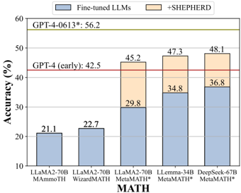
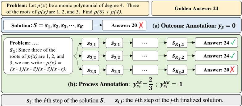
Figure 1: We evaluate the performance of various LLMs with MATH-SHEPHERD on the GSM8K and MATH datasets. All base models are finetuned with the MetaMath dataset (Yu et al., 2023b). The +SHEPHERD results are obtained by selecting the best one from 256 candidates using MATHSHEPHERD. We observe that MATH-SHEPHERD is compatible with different LLMs. The results of GPT-4 (early) are from Bubeck et al. (2023).
<details>
<summary>Image 2 Details</summary>
### Visual Description
## Bar Chart: Model Accuracy Comparison on GSM8K Dataset
### Overview
This is a grouped bar chart comparing the accuracy percentages of five different large language models (LLMs) on the GSM8K mathematical reasoning benchmark. Each model is evaluated under two conditions: as a "Fine-tuned LLM" (blue bars) and with the addition of "+SHEPHERD" (orange bars). Two horizontal red lines provide performance benchmarks for GPT-4 models.
### Components/Axes
* **Chart Type:** Grouped vertical bar chart.
* **Y-Axis:** Labeled "Accuracy (%)". Scale ranges from 70 to 95, with major tick marks every 5 units (70, 75, 80, 85, 90, 95).
* **X-Axis:** Labeled "GSM8K". It lists five distinct model configurations:
1. `LLaMA2-70b MAMoTH`
2. `LLaMA2-70b WizardMATH`
3. `LLaMA2-70b MetaMath*`
4. `LLaMA-34b MetaMath*`
5. `DeepSeek-67b MetaMath*`
* **Legend:** Positioned at the top center of the chart area.
* A blue square corresponds to the label "Fine-tuned LLMs".
* An orange square corresponds to the label "+SHEPHERD".
* **Benchmark Lines:** Two solid red horizontal lines span the chart width.
* The upper line is labeled `GPT-4-0613*: 94.4` at its left end.
* The lower line is labeled `GPT-4 (early): 92.0` at its left end.
### Detailed Analysis
The chart presents paired data for each of the five models. The blue bar represents the baseline fine-tuned model's accuracy, and the orange bar represents the accuracy after applying the SHEPHERD method.
1. **LLaMA2-70b MAMoTH:**
* Fine-tuned LLMs (Blue): 72.4%
* +SHEPHERD (Orange): 81.6%
* **Trend:** A significant upward increase of approximately 9.2 percentage points.
2. **LLaMA2-70b WizardMATH:**
* Fine-tuned LLMs (Blue): 81.6%
* +SHEPHERD (Orange): 93.2%
* **Trend:** A substantial upward increase of approximately 11.6 percentage points.
3. **LLaMA2-70b MetaMath*:**
* Fine-tuned LLMs (Blue): 80.4%
* +SHEPHERD (Orange): 90.9%
* **Trend:** A strong upward increase of approximately 10.5 percentage points.
4. **LLaMA-34b MetaMath*:**
* Fine-tuned LLMs (Blue): 75.8%
* +SHEPHERD (Orange): 90.9%
* **Trend:** A very large upward increase of approximately 15.1 percentage points.
5. **DeepSeek-67b MetaMath*:**
* Fine-tuned LLMs (Blue): 82.8%
* +SHEPHERD (Orange): 93.3%
* **Trend:** A strong upward increase of approximately 10.5 percentage points.
**Benchmark Comparison:**
* The `GPT-4 (early)` benchmark is at 92.0%.
* The `GPT-4-0613*` benchmark is at 94.4%.
* With SHEPHERD, three models (LLaMA2-70b WizardMATH, LLaMA2-70b MetaMath*, DeepSeek-67b MetaMath*) achieve accuracy at or above the `GPT-4 (early)` benchmark.
* The highest performing model configuration is `DeepSeek-67b MetaMath* +SHEPHERD` at 93.3%, which is 1.1 percentage points below the `GPT-4-0613*` benchmark.
### Key Observations
1. **Universal Improvement:** The addition of SHEPHERD results in a consistent and substantial accuracy improvement for every single model tested. The improvement ranges from ~9.2 to ~15.1 percentage points.
2. **Performance Tier:** The SHEPHERD-enhanced models cluster in a high-performance tier between 90.9% and 93.3%, while the baseline fine-tuned models are more spread out between 72.4% and 82.8%.
3. **Model Comparison:** Among the baseline fine-tuned models, `DeepSeek-67b MetaMath*` (82.8%) and `LLaMA2-70b WizardMATH` (81.6%) perform best. With SHEPHERD, `DeepSeek-67b MetaMath*` (93.3%) and `LLaMA2-70b WizardMATH` (93.2%) remain the top performers.
4. **Benchmark Proximity:** The SHEPHERD method enables several open-weight models to reach performance levels competitive with early and mid-2023 versions of a leading proprietary model (GPT-4).
### Interpretation
This chart demonstrates the potent effect of the SHEPHERD technique as a performance multiplier for fine-tuned LLMs on mathematical reasoning tasks. The data suggests that SHEPHERD is not merely an incremental improvement but a transformative one, consistently bridging a significant portion of the gap between various fine-tuned models and the GPT-4 benchmark.
The fact that models of different sizes (34b, 67b, 70b) and from different fine-tuning families (MAMoTH, WizardMATH, MetaMath*) all show dramatic gains indicates that SHEPHERD likely addresses a fundamental limitation in the reasoning or problem-solving process of the base fine-tuned models, rather than being a narrow fix for a specific model architecture.
The narrowing of the performance spread among the SHEPHERD-enhanced models (90.9% - 93.3%) compared to the baselines (72.4% - 82.8%) implies that the technique may help models converge toward a higher performance ceiling on this benchmark, potentially by instilling a more robust and generalizable reasoning methodology. The results position SHEPHERD as a highly valuable method for elevating the capabilities of open-weight models to compete with state-of-the-art proprietary systems on complex reasoning benchmarks.
</details>
<details>
<summary>Image 3 Details</summary>
### Visual Description
## Bar Chart: Performance on MATH Benchmark with and without SHEPHERD Augmentation
### Overview
The image is a grouped, stacked bar chart comparing the accuracy of various Large Language Models (LLMs) on the "MATH" benchmark. It specifically contrasts the performance of models that have been fine-tuned on mathematical tasks ("Fine-tuned LLMs") against the performance of those same models when augmented with a method called "SHEPHERD" ("+SHEPHERD"). Two horizontal reference lines indicate the performance of GPT-4 variants.
### Components/Axes
* **Chart Type:** Grouped, stacked bar chart.
* **Y-Axis:** Labeled "Accuracy (%)". Scale runs from 10 to 60, with major tick marks every 10 units.
* **X-Axis:** Labeled "MATH". It lists five distinct model configurations:
1. `LLaMA2-70B MAMoTH`
2. `WizardMATH`
3. `LLaMA2-70B MetaMath*`
4. `Llemma-34B MetaMath*`
5. `DeepSeek-67B MetaMath*`
* **Legend:** Located at the top center of the chart area.
* A blue rectangle corresponds to "Fine-tuned LLMs".
* An orange rectangle corresponds to "+SHEPHERD".
* **Reference Lines:**
* A solid red horizontal line at approximately 42.5% accuracy, labeled "GPT-4 (early): 42.5".
* A solid yellow-green horizontal line at approximately 56.2% accuracy, labeled "GPT-4-0613*: 56.2".
### Detailed Analysis
The chart presents data for five model configurations. Each bar is stacked, with the blue segment representing the base fine-tuned model's accuracy and the orange segment representing the additional accuracy gained by applying SHEPHERD.
1. **LLaMA2-70B MAMoTH:**
* **Fine-tuned LLMs (Blue):** 21.1%
* **+SHEPHERD (Orange):** 0% (No orange segment is visible).
* **Total Accuracy:** 21.1%
2. **WizardMATH:**
* **Fine-tuned LLMs (Blue):** 22.7%
* **+SHEPHERD (Orange):** 0% (No orange segment is visible).
* **Total Accuracy:** 22.7%
3. **LLaMA2-70B MetaMath*:**
* **Fine-tuned LLMs (Blue):** 29.8%
* **+SHEPHERD (Orange):** 15.4% (Calculated as 45.2% total - 29.8% base).
* **Total Accuracy:** 45.2%
4. **Llemma-34B MetaMath*:**
* **Fine-tuned LLMs (Blue):** 34.8%
* **+SHEPHERD (Orange):** 12.5% (Calculated as 47.3% total - 34.8% base).
* **Total Accuracy:** 47.3%
5. **DeepSeek-67B MetaMath*:**
* **Fine-tuned LLMs (Blue):** 36.8%
* **+SHEPHERD (Orange):** 11.3% (Calculated as 48.1% total - 36.8% base).
* **Total Accuracy:** 48.1%
**Trend Verification:**
* **Base Models (Blue Segments):** The trend slopes upward from left to right. Accuracy increases from 21.1% (LLaMA2-70B MAMoTH) to 36.8% (DeepSeek-67B MetaMath*), indicating that the choice of base model and its specific fine-tuning (MAMoTH vs. WizardMATH vs. MetaMath*) significantly impacts baseline performance.
* **SHEPHERD Augmentation (Orange Segments):** SHEPHERD is only applied to the last three models (those using MetaMath* fine-tuning). For these, it provides a consistent positive boost, though the magnitude of the boost decreases slightly as the base model's performance increases (from +15.4% to +11.3%).
### Key Observations
1. **SHEPHERD's Impact:** The SHEPHERD method provides a substantial and consistent accuracy improvement for models fine-tuned with MetaMath*, boosting performance by between 11.3 and 15.4 percentage points.
2. **Model Hierarchy:** Among the tested configurations, `DeepSeek-67B MetaMath* + SHEPHERD` achieves the highest accuracy at 48.1%. The `LLaMA2-70B MetaMath* + SHEPHERD` configuration (45.2%) surpasses the `GPT-4 (early)` benchmark (42.5%).
3. **Benchmark Gap:** All tested model configurations, even the best-performing one (48.1%), remain below the performance of `GPT-4-0613*` (56.2%).
4. **Fine-tuning Method Matters:** Models fine-tuned with MetaMath* (columns 3-5) show significantly higher baseline performance (29.8%-36.8%) compared to those fine-tuned with MAMoTH or WizardMATH (21.1%-22.7%).
### Interpretation
This chart demonstrates the efficacy of the SHEPHERD augmentation technique for improving mathematical reasoning in LLMs. The data suggests that SHEPHERD is not a standalone solution but a powerful complementary method that builds upon a strong fine-tuned foundation (specifically, MetaMath* fine-tuning in this experiment).
The consistent upward trend in the blue bars indicates that advancements in base model architecture (e.g., DeepSeek vs. LLaMA) and fine-tuning methodology (MetaMath* vs. others) are primary drivers of performance. SHEPHERD then acts as a performance multiplier on top of these advances.
The fact that the best composite model still falls short of GPT-4-0613* highlights the continued gap between specialized, open-weight models and the capabilities of large, proprietary systems on complex reasoning tasks. However, the chart also shows a promising trajectory: by combining strong fine-tuning (MetaMath*) with targeted augmentation (SHEPHERD), smaller models can approach and even surpass earlier versions of state-of-the-art models like GPT-4 (early). This points to a viable pathway for developing more efficient and accessible high-performance AI systems for specialized domains like mathematics.
</details>
† Contribution during internship at DeepSeek-AI.
## 1 INTRODUCTION
Large language models (LLMs) have demonstrated remarkable capabilities across various tasks (Park et al., 2023; Kaddour et al., 2023; Song et al.; Li et al., 2023a; Wang et al., 2023a; Chen et al., 2023; Zheng et al., 2023; Wang et al., 2023c), However, even the most advanced LLMs face challenges in complex multi-step mathematical reasoning problems (Lightman et al., 2023; Huang et al., 2023). To address this issue, prior research has explored different methodologies, such as pretraining (Azerbayev et al., 2023), fine-tuning (Luo et al., 2023; Yu et al., 2023b; Wang et al., 2023b), prompting (Wei et al., 2022; Fu et al., 2022), and verification (Wang et al., 2023d; Li et al., 2023b; Zhu et al., 2023; Leviathan et al., 2023). Among these techniques, verification has recently emerged as a favored method. The motivation behind verification is that relying solely on the top-1 result may not always produce reliable outcomes. A verification model can rerank candidate responses, ensuring higher accuracy and consistency in the outputs of LLMs. In addition, a good verification model can also offer invaluable feedback for further improvement of LLMs (Uesato et al., 2022; Wang et al., 2023b; Pan et al., 2023).
The verification models generally fall into the outcome reward model (ORM) (Cobbe et al., 2021; Yu et al., 2023a) and process reward model (PRM) (Li et al., 2023b; Uesato et al., 2022; Lightman et al., 2023; Ma et al., 2023). The ORM assigns a confidence score based on the entire generation sequence, whereas the PRM evaluates the reasoning path step-by-step. PRM is advantageous due to several compelling reasons. One major benefit is its ability to offer precise feedback by identifying the specific location of any errors that may arise, which is a valuable signal in reinforcement learning and automatic correction. Besides, The PRM exhibits similarities to human behavior when assessing a reasoning problem. If any steps contain an error, the final result is more likely to be incorrect, mirroring the way human judgment works. However, gathering data to train a PRM can be an arduous process. Uesato et al. (2022) and Lightman et al. (2023) utilize human annotators to provide process supervision annotations, enhancing the performance of PRM. Nevertheless, annotation by humans, particularly for intricate multi-step reasoning tasks that require advanced annotator skills, can be quite costly, which hinders the advancement and practical application of PRM.
To tackle the problem, in this paper, we propose an automatic process annotation framework. Inspired by Monte Carlo Tree Search (Kocsis & Szepesv´ ari, 2006; Coulom, 2006; Silver et al., 2016; ´ Swiechowski et al., 2023), we define the quality of an intermediate step as its potential to deduce the correct final answer. By leveraging the correctness of the answer, we can automatically gather step-wise supervision. Specifically, given a math problem with a golden answer and a step-by-step solution, to achieve the label of a specific step, we utilize a fine-tuned LLM to decode multiple subsequent reasoning paths from this step. We further validate whether the decoded final answer matches with the golden answer. If a reasoning step can deduce more correct answers than another, it would be assigned a higher correctness score.
We use this automatic way to construct the training data for MATH-SHEPHERD, and verify our ideas on two widely used mathematical benchmarks, GSM8K (Cobbe et al., 2021) and MATH (Hendrycks et al., 2021). We explore the effectiveness of MATH-SHEPHERD in two scenarios: 1) verification: MATH-SHEPHERD is utilized for reranking multiple outputs generated by LLMs; 2) reinforcement learning: MATH-SHEPHERD is employed to reinforce LLMs with step-by-step Proximal Policy Optimization (PPO). With the verification of MATH-SHEPHERD, a series of open-source LLMs from 7B to 70B demonstrates exceptional performance. For instance, the step-by-step PPO with MATHSHEPHERD significantly improves the accuracy of Mistral-7B (77.9% → 84.1% on GSM8K and 28.6% → 33.0% on MATH). The accuracy can be further enhanced to 89.1% and 43.5% on GSM8K and MATH with verification. DeepSeek 67B (DeepSeek, 2023) achieves accuracy rates of 93.3% on the GSM8K dataset and 48.1% on the MATH dataset with verification of MATH-SHEPHERD. To the best of our knowledge, these results are unprecedented for open-source models that do not rely on additional tools.
Our main contributions are as follows:
1) We propose a framework to automatically construct process supervision datasets without human annotations for math reasoning tasks.
- 2) We evaluate our method on both step-by-step verification and reinforcement learning scenarios. Extensive experiments on two widely used mathematical benchmarks - GSM8K and MATH, in addition to a series of LLMs ranging from 7B to 70B, demonstrate the effectiveness of our method.
- 3) We empirically analyze the key factors for training high-performing process reward models, shedding light on future directions toward improving reasoning capability with automatic step-bystep verification and supervision.
## 2 RELATED WORKS
Improving and eliciting mathematical reasoning abilities of LLMs. Mathematical reasoning tasks are one of the most challenging tasks for LLMs. Researchers have proposed various methods to improve or elicit the mathematical reasoning ability of LLMs, which can be broadly divided into three groups: 1) pre-training : The pre-training methods (OpenAI, 2023; Anil et al., 2023; Touvron et al., 2023; Azerbayev et al., 2023) pre-train LLMs on a vast of datasets that are related to math problems, such as the Proof-Pile and ArXiv (Azerbayev et al., 2023) with a simple next token prediction objective. 2) fine-tuning : The fine-tuning methods (Yu et al., 2023b; Luo et al., 2023; Yue et al., 2023; Wang et al., 2023b; Gou et al., 2023) can also enhance the mathematical reasoning ability of LLMs. The core of fine-tuning usually lies in constructing high-quality question-response pair datasets with a chain-of-thought reasoning process. and 3) prompting : The prompting methods (Wei et al., 2022; Zhang et al., 2023; Fu et al., 2022; Bi et al., 2023) aim to elicit the mathematical reasoning ability of LLMs by designing prompting strategy without updating the model parameters, which is very convenient and practical.
Mathematical reasoning verification for LLMs. Except for directly improving and eliciting the mathematical reasoning potential of LLMs, the reasoning results can be boosted via an extra verifier for selecting the best answer from multiple decoded candidates. There are two primary types of verifiers: the Outcome Reward Model (ORM) and the Process Reward Model (PRM). The ORM allocates a score to the entire solution while the PRM assigns a score to each individual step in the reasoning process. Recent findings by (Lightman et al., 2023) suggest that PRM outperforms ORM. In addition to verification, reward models can offer invaluable feedback for further training of generators (Uesato et al., 2022; Pan et al., 2023). Compared to ORM, PRM provides more detailed feedback, demonstrating greater potential to enhance generator (Wu et al., 2023). However, training a PRM requires access to expensive human-annotated datasets (Uesato et al., 2022; Lightman et al., 2023), which hinders the advancement and practical application of PRM. Therefore, in this paper, we aim to build a PRM for mathematical reasoning without human annotation, and we explore the effectiveness of the automatic PRM with both verification and reinforcement learning scenarios.
## 3 METHODOLOGY
In this section, we first present our task formulation to evaluate the performance of reward models (§3.1). Subsequently, we outline two typical categories of reward models, ORM and PRM(§3.2). Then, we introduce our methodology to automatically build the training dataset for PRM(§3.3), breaking the bottleneck of heavy reliance on manual annotation in existing work (Uesato et al., 2022; Lightman et al., 2023).
## 3.1 TASK FORMULATION
We evaluate the performance of the reward model in two scenarios:
Verification Following (Lightman et al., 2023), we consider a best-of-N selection evaluation paradigm. Specifically, given a problem p in the testing set, we sample N candidate solutions from a generator. These candidates are then scored using a reward model, and the highest-scoring solution is selected as the final answer. An enhanced reward model elevates the likelihood of selecting the solution containing the correct answer, consequently raising the success rate in solving mathematical problems for LLMs.
Reinforcement learning We also use the automatically constructed PRM to supervise LLMs with step-by-step PPO. In this scenario, we evaluate the accuracy of the LLMs' greedy decoding output. An enhanced reward model is instrumental in training higher-performing LLMs.
## 3.2 REWARD MODELS FOR MATHEMATICAL PROBLEM
ORM Given a mathematical problem p and its solution s , ORM ( P × S → R ) assigns a single real-value to s to indicate whether s is correct. ORM is usually trained with a cross-entropy loss (Cobbe et al., 2021; Li et al., 2023b):
$$\displaystyle \sum _ { i = 1 } ^ { n } L _ { i s } ( 1 )$$
where y s is the golden answer of the solution s , y s = 1 if s is correct, otherwise y s = 0 . r s is the sigmoid score of s assigned by ORM. The success of the reward model hinges on the effective construction of the high-quality training dataset. As the math problem usually has a certain answer, we can automatically construct the training set of ORM by two steps: 1) sampling some candidate solutions for a problem from a generator; 2) assigning the label to each sampling solution by checking whether its answer is correct. Although false positives solutions that reach the correct answer with incorrect reasoning will be misgraded, previous studies have proven that it is still effective for training a good ORM (Lightman et al., 2023; Yu et al., 2023a).
PRM Take a step further, PRM ( P × S → R + ) assigns a score to each reasoning step of s , which is usually trained with:
$$\sum _ { i = 1 } ^ { K } y _ { s _ { i } } \log r _ { s _ { i } } + ( 1 - y _ { s _ { i } } )$$
where y s i is the golden answer of s i (the i -th step of s ), r s i is the sigmoid score of s i assigned by PRM and K is the number of reasoning steps for s . (Lightman et al., 2023) also conceptualizes the PRM training as a three-class classification problem, in which each step is classified as either 'good', 'neutral', or 'bad'. In this paper, we found that there is not much difference between the binary and the three classifications, and we regard PRM training as the binary classification. Compared to ORM, PRM can provide more detailed and reliable feedback (Lightman et al., 2023). However, there are currently no automated methods available for constructing high-quality PRM training datasets. Previous works (Uesato et al., 2022; Lightman et al., 2023) typically resort to costly human annotations. While PRM manages to outperform ORM (Lightman et al., 2023), the annotation cost invariably impedes both the development and application of PRM.
## 3.3 AUTOMATIC PROCESS ANNOTATION
In this section, we propose an automatic process annotation framework to mitigate the annotation cost issues associated with PRM. We first define the quality of a reasoning step, followed by the introduction of our solution that obviates the necessity for human annotation.
## 3.3.1 DEFINITION
Inspired by Monto Carlo Tree Search (Kocsis & Szepesv´ ari, 2006; Coulom, 2006; Silver et al., 2016; ´ Swiechowski et al., 2023), we define the quality of a reasoning step as its potential to deduce the correct answer. This criterion stems from the primary objective of the reasoning process, which essentially is a cognitive procedure aiding humans or intelligent agents in reaching a well-founded outcome (Huang & Chang, 2023). Therefore, a step that has the potential to deduce a well-founded result can be considered a good reasoning step. Analogous to ORM, this definition also introduces some degree of noise. Nevertheless, we find that it is beneficial for effectively training a good PRM.
## 3.3.2 SOLUTION
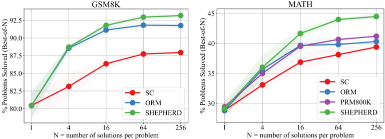
Completion To quantify and estimate the potential for a give reasoning step s i , as shown in Figure 2, we use a 'completer' to finalize N subsequent reasoning processes from this step: { ( s i +1 ,j , · · · , s K j ,j , a j ) } N j =1 , where a j and K j are the decoded answer and the total number of steps for the j -th finalized solution, respectively. Then, we estimate the potential of this step based on the correctness of all decoded answers A = { a j } N j =1 .
Figure 2: Comparison for previous automatic outcome annotation and our automatic process annotation. (a): automatic outcome annotation assigns a label to the entire solution S , dependent on the correctness of the answer; (b) automatic process annotation employs a 'completer' to finalize N reasoning processes (N=3 in this figure) for an intermediate step ( s 1 in this figure), subsequently use hard estimation (HE) and soft estimation (SE) to annotate this step based on all decoded answers.
<details>
<summary>Image 4 Details</summary>
### Visual Description
\n
## Diagram: Mathematical Solution Process Annotation
### Overview
The image is a technical diagram illustrating two methods of annotating and evaluating the solution process for a specific mathematical problem. It contrasts a simple outcome-based annotation with a more granular process-based annotation, using a concrete example to demonstrate how different solution paths can lead to correct or incorrect final answers.
### Components/Axes
The diagram is organized into several distinct regions:
1. **Header Region (Top):**
* **Problem Statement (Top-Left):** "Problem: Let \( p(x) \) be a monic polynomial of degree 4. Three of the roots of \( p(x) \) are 1, 2, and 3. Find \( p(0) + p(4) \)."
* **Golden Answer (Top-Right):** "Golden Answer: 24"
2. **Main Process Region (Center):**
* **Part (a) Outcome Annotation:** A single horizontal flow.
* Input: "Solution: \( S = s_1, s_2, s_3, \cdots, s_K \)"
* Process: An arrow points to a box containing "Answer: 20 ❌".
* Annotation Label: "(a) Outcome Annotation: \( y_S = 0 \)"
* **Part (b) Process Annotation:** A branching flow showing multiple solution attempts.
* **Root Problem Box (Left):** "Problem: ...."
* **First Step Box (\( s_1 \)):** "\( s_1 \); Since three of the roots of \( p(x) \) are 1, 2, and 3, we can write: \( p(x) = (x-1)(x-2)(x-3)(x-r) \)."
* **Branching Paths:** Three parallel horizontal flows originate from the \( s_1 \) box, labeled for \( j = 1, 2, 3 \).
* **Path j=1 (Top):** \( s_{2,1} \rightarrow s_{3,1} \rightarrow \cdots \rightarrow s_{K,1} \) leading to "Answer: 24 ✅".
* **Path j=2 (Middle):** \( s_{2,2} \rightarrow s_{3,2} \rightarrow \cdots \rightarrow s_{K,2} \) leading to "Answer: 24 ✅".
* **Path j=3 (Bottom):** \( s_{2,3} \rightarrow s_{3,3} \rightarrow \cdots \rightarrow s_{K,3} \) leading to "Answer: 20 ❌".
* **Annotation Label:** "(b): Process Annotation: \( y_{s_1}^{SE} = \frac{2}{3} \) ; \( y_{s_1}^{HE} = 1 \)"
3. **Footer/Legend Region (Bottom):**
* **Legend:** "\( s_i \): the \( i \)-th step of the solution \( S \). \( s_{i,j} \): the \( i \)-th step of the \( j \)-th finalized solution."
### Detailed Analysis
* **Problem & Solution:** The core problem involves finding the value of \( p(0) + p(4) \) for a monic quartic polynomial with known roots 1, 2, and 3. The "Golden Answer" is established as 24.
* **Outcome Annotation (a):** This evaluates the entire solution process \( S \) as a single unit. The final answer derived is 20, which is incorrect (marked with ❌). The annotation \( y_S = 0 \) likely represents a binary score (0 for incorrect, 1 for correct).
* **Process Annotation (b):** This evaluates the first critical step \( s_1 \) of the solution. The step \( s_1 \) correctly sets up the polynomial form \( p(x) = (x-1)(x-2)(x-3)(x-r) \). From this single correct starting point, three distinct "finalized solutions" (j=1,2,3) are shown.
* Two of these paths (j=1 and j=2) lead to the correct answer of 24 (✅).
* One path (j=3) leads to the incorrect answer of 20 (❌).
* **Process Metrics:** Two metrics are derived from this branching:
* \( y_{s_1}^{SE} = \frac{2}{3} \): This appears to be a "Success Efficiency" or similar metric, calculated as the ratio of correct final answers (2) to total attempted paths (3) stemming from step \( s_1 \).
* \( y_{s_1}^{HE} = 1 \): This likely represents a "Human Efficiency" or "Heuristic Efficiency" score, possibly indicating that the initial step \( s_1 \) itself is fundamentally correct or optimal, regardless of subsequent errors in some paths.
### Key Observations
1. **Divergence from a Common Start:** All three solution paths share the identical, correct first step (\( s_1 \)). The divergence into correct and incorrect outcomes must therefore occur in the subsequent steps (\( s_{2,j} \) onwards).
2. **Annotation Granularity:** The diagram highlights the difference between evaluating only the final output (Outcome Annotation) versus evaluating the quality of a pivotal intermediate step (Process Annotation).
3. **Visual Coding:** Correct answers are consistently marked with green checkmarks (✅) and incorrect ones with red crosses (❌). The branching structure in part (b) is visually clear, with arrows indicating the flow of reasoning.
### Interpretation
This diagram serves as a conceptual model for evaluating problem-solving processes, particularly in educational or AI training contexts. It argues that judging a solution solely by its final answer (Outcome Annotation) can be misleading. A student or an AI model might start with a perfectly valid strategy (step \( s_1 \)) but make an error later, resulting in a wrong answer. The Process Annotation method focuses on the quality of that critical initial step.
The metrics \( y_{s_1}^{SE} \) and \( y_{s_1}^{HE} \) suggest a framework for quantifying the robustness or reliability of a given solution step. A step that leads to a correct answer 2 out of 3 times (\( SE = 2/3 \)) might be considered good but not foolproof, while a step that is fundamentally sound (\( HE = 1 \)) is valuable even if some execution paths fail. The diagram implies that for effective learning or model training, feedback should be directed at these pivotal decision points (like \( s_1 \)) rather than just the final outcome. It visually advocates for a more nuanced, process-oriented assessment of mathematical reasoning.
</details>
Estimation In this paper, we use two methods to estimate the quality y s i for the step s i , hard estimation (HE) and soft estimation (SE). HE supposes that a reasoning step is good as long as it can reach the correct answer a ∗ :
$$y _ { s _ { 1 } } = \int _ { 0 } ^ { 1 } z _ { a _ { j } } \in A , y _ { j } = a *$$
SE assumes the quality of a step as the frequency with which it reaches the correct answer:
$$y _ { s } = \frac { \sum _ { j = 1 } ^ { N } y _ { j } = 1 ( a _ { j } = a * ) } { N } .$$
Once we gather the label of each step, we can train PRM with the cross-entropy loss. In conclusion, our automatic process annotation framework defines the quality of a step as its potential to deduce the correct answer and achieve the label of each step by completion and estimation.
## 3.4 RANKING FOR VERIFICATION
Following (Lightman et al., 2023), we use the minimum score across all steps to represent the final score of a solution assigned by PRM. We also explore the combination of self-consistency and reward models following (Li et al., 2023b). In this context, we initially classify solutions into distinct groups according to their final answers. Following that, we compute the aggregate score for each group. Formally, the final prediction answer based on N candidate solutions is:
$$a _ { sc + r m } = \arg _ { a } \max _ { i = 1 } ^ { N } \sum _ { i = 1 } ^ { N } I ( a _ { i } = a ) .$$
Where RM ( p, S i ) is the score of the i -th solution assigned by ORM or PRM for problem p .
## 3.5 REINFORCE LEARNING WITH PROCESS SUPERVISION
Upon achieving PRM, we employ reinforcement learning to train LLMs. We implement Proximal Policy Optimization (PPO) in a step-by-step manner. This method differs from the conventional strategy that utilizes PPO with ORM, which only offers a reward at the end of the response. Conversely, our step-by-step PPO offers rewards at the end of each reasoning step.
Table 1: Performances of different LLMs on GSM8K and MATH with different verification strategies. The reward models are trained based on LLama2-70B and LLemma-34B on GSM8K and MATH, respectively. The verification is based on 256 outputs.
| Models | Verifiers | GSM8K | MATH500 |
|------------------------|-----------------------------------------|---------|-----------|
| LLaMA2-70B: MetaMATH | Self-Consistency | 88 | 39.4 |
| LLaMA2-70B: MetaMATH | ORM | 91.8 | 40.4 |
| LLaMA2-70B: MetaMATH | Self-Consistency+ORM | 92 | 42 |
| LLaMA2-70B: MetaMATH | MATH-SHEPHERD (Ours) | 93.2 | 44.5 |
| LLaMA2-70B: MetaMATH | Self-Consistency + MATH-SHEPHERD (Ours) | 92.4 | 45.2 |
| LLemma-34B: MetaMATH | Self-Consistency | 82.6 | 44.2 |
| LLemma-34B: MetaMATH | ORM | 90 | 43.7 |
| LLemma-34B: MetaMATH | Self-Consistency+ORM | 89.6 | 45.4 |
| LLemma-34B: MetaMATH | MATH-SHEPHERD (Ours) | 90.9 | 46 |
| LLemma-34B: MetaMATH | Self-Consistency + MATH-SHEPHERD (Ours) | 89.7 | 47.3 |
| DeepSeek-67B: MetaMATH | Self-Consistency | 88.2 | 45.4 |
| DeepSeek-67B: MetaMATH | ORM | 92.6 | 45.3 |
| DeepSeek-67B: MetaMATH | Self-Consistency+ORM | 92.4 | 47 |
| DeepSeek-67B: MetaMATH | MATH-SHEPHERD (Ours) | 93.3 | 47 |
| DeepSeek-67B: MetaMATH | Self-Consistency + MATH-SHEPHERD (Ours) | 92.5 | 48.1 |
## 4 EXPERIMENTS
Datasets We conduct our experiments using two widely used math reasoning datasets, GSM8K (Cobbe et al., 2021) and MATH (Hendrycks et al., 2021). For the GSM8K dataset, we leverage the whole test set in both verification and reinforcement learning scenarios. For the MATH dataset, in the verification scenario, due to the computation cost, we employ a subset MATH500 that is identical to the test set of Lightman et al. (2023). The subset consists of 500 representative problems, and we find that the subset evaluation produces similar results to the full-set evaluation. To assess different verification methods, we generate 256 candidate solutions for each test problem. We report the mean accuracy of 3 groups of sampling results. In the reinforcement learning scenario, we use the whole test set to evaluate the model performance. We train LLMs with MetaMATH (Yu et al., 2023b).
Parameter Setting Our experiments are based on a series of large language models, LLaMA27B/13B/70B (Touvron et al., 2023), LLemma-7B/34B (Azerbayev et al., 2023), Mistral-7B (Jiang et al., 2023) and DeepSeek-67B (DeepSeek, 2023). We train the generator and completer for 3 epochs on MetaMATH. We train the Mistral-7B with a learning rate of 5e-6. For other models, The learning rates are set to 2e-5, 1e-5, and 6e-6 for the 7B/13B, 34B, and 67B/70B LLMs, respectively. To construct the training dataset of ORM and PRM, we train 7B and 13B models for a single epoch on the GSM8K and MATH training sets. Subsequently, we sample 15 solutions per problem from each model for the training set. Following this, we eliminate duplicate solutions and annotate the solutions at each step. We use LLemma-7B as the completer with the decoded number N=8. Consequently, we obtain around 170k solutions for GSM8K and 270k solutions for MATH. For verification, we choose LLaMA2-70B and LLemma-34B as the base models to train reward models for GSM8K and MATH, respectively. For reinforcement learning, we choose Mistral-7B as the base model to train reward models and use it to supervise LLama2-7B and Mistral-7B generators. The reward model is trained in 1 epoch with a learning rate 1e-6. For the sake of convenience, we train the PRM using the hard estimation version because it allows us to utilize a standard language modeling pipeline by selecting two special tokens to represent 'has potential' and 'no potential' labels, thereby eliminating the need for any specific model adjustments. In reinforcement learning, the learning rate is 4e-7 and 1e-7 for LLaMA2-7B and Mistral-7B, respectively. The Kullback-Leibler coefficient is set to 0.04. We implement a cosine learning rate scheduler, employing a minimal learning rate set to 1e-8. We use 3D parallelism provided by hfai 1 to train all models with the max sequence length of 512.
1 https://doc.hfai.high-flyer.cn/index.html
Table 2: Performances of different 7B models on GSM8K and MATH with greedy decoding. We use the questions in MetaMATH for RFT and PPO training. Both LLaMA2-7B and Mistral-7B are supervised by Mistral-7B-ORM and -MATH-SHEPHERD.
| Models | GSM8K | MATH |
|-----------------------------------------|---------|--------|
| LLaMA2-7B: MetaMATH | 66.6 | 19.2 |
| + RFT | 68.5 | 19.9 |
| + ORM-PPO | 70.8 | 20.8 |
| + MATH-SHEPHERD-step-by-step-PPO (Ours) | 73.2 | 21.6 |
| Mistral-7B: MetaMATH | 77.9 | 28.6 |
| + RFT | 79 | 29.9 |
| + ORM-PPO | 81.8 | 31.3 |
| + MATH-SHEPHERD-step-by-step-PPO (Ours) | 84.1 | 33 |
Baselines and Metrics In the verification scenario, following (Lightman et al., 2023), we evaluate the performance of our reward model by comparing it against the Self-consistency (majority voting) and outcome reward model. The accuracy of the best-of-N solution is utilized as the evaluation metric. For PRM, the minimum score across all steps is adopted to represent the final score of a solution. In the reinforcement scenario, we compare our step-by-step supervision with the outcome supervision provided by ORM, and Rejective Sampling Fine-tuning (RFT) (Yuan et al., 2023), we sample 8 responses for each question in MetaMATH for RFT. We use the accuracy of LLMs' greedy decoding output to assess the performance.
## 4.1 MAIN RESULTS
MATH-SHEPHERD as verifier Table 1 presents the performance comparison of various methods on GSM8K and MATH. We find that: 1) As the verifier, MATH-SHEPHERD consistently outperforms self-consistency and ORM on two datasets with all generators. Specifically, enhanced by MATHSHEPHERD, DeepSeek-67B achieves 93.3% and 48.1% accuracy on GSM8K and MATH; 2) In comparison to GSM8K, PRM achieves a greater advantage over ORM on the more challenging MATH dataset; This outcome aligns with the findings in Uesato et al. (2022) and Lightman et al. (2023). The former discovers that PRM and ORM yield similar results on GSM8K, whereas the latter shows that PRM significantly outperforms ORM on the MATH dataset. This could be attributed to the relative simplicity of the GSM8K dataset compared to MATH, i.e., the GSM8K dataset necessitates fewer steps for problem-solving. As a result, ORM operates efficiently when handling this particular dataset; 3) In GSM8K, when combined with self-consistency, there's a drop in performance, whereas in MATH, performance improves. These results indicate that if the reward model is sufficiently powerful for a task, combining it with self-consistency may harm the verification performance.
MATH-SHEPHERD as reward model on reinforcement learning Table 2 presents the performance of different LLMs with greedy decoding outputs. As is shown: 1) step-by-step PPO significantly improves the performance of two supervised fine-tuned models. For example, Mistral-7B with step-by-step PPO achieves 84.1% and 33.0% on the GSM8K and MATH datasets, respectively; 2) RFT only slightly improves the model performance, we believe this is because MetaMATH already has conducted some data augmentation strategies like RFT; 3) the vanilla PPO with ORM can also enhance the model performance. However, it does not perform as well as the step-by-step PPO supervised by MATH-SHEPHERD, demonstrating the potential of step-by-step supervision.
MATH-SHEPHERD as both reward models and verifiers We also combine the reinforcement learning and the verification. As shown in Table 3: 1) reinforcement learning and verification are complementary. For example, in MATH, step-by-step PPO Mistral-7B outperforms supervised fine-tuning Mistral-7B 7.2% accuracy with self-consistency as the verifier; The performance gap is even larger than that of greedy decoding results, i.e., 4.4%; 2) after reinforcement learning, the vanilla verification methods with only reward models is inferior to self-consistency, we think the
Table 3: Results of reinforcement learning and verification combination. The reward models are trained based on Mistral-7B. The verification is based on 256 outputs.
| Models | Verifiers | GSM8K | MATH500 |
|--------------------------|-----------------------------------------|---------|-----------|
| Mistral-7B: MetaMATH | Self-Consistency | 83.9 | 35.1 |
| Mistral-7B: MetaMATH | ORM | 86.2 | 36.4 |
| Mistral-7B: MetaMATH | Self-Consistency+ORM | 86.6 | 38 |
| Mistral-7B: MetaMATH | MATH-SHEPHERD (Ours) | 87.1 | 37.3 |
| Mistral-7B: MetaMATH | Self-Consistency + MATH-SHEPHERD (Ours) | 86.3 | 38.3 |
| Mistral-7B: MetaMATH | Self-Consistency | 87.4 | 42.3 |
| Mistral-7B: MetaMATH | ORM | 87.6 | 41.3 |
| +step-by-step PPO (Ours) | Self-Consistency+ORM | 89 | 43.1 |
| +step-by-step PPO (Ours) | MATH-SHEPHERD (Ours) | 88.4 | 41.1 |
| +step-by-step PPO (Ours) | Self-Consistency + MATH-SHEPHERD (Ours) | 89.1 | 43.5 |
reason is that the initial reward model is not sufficient to supervise the more powerful model after PPO. These results can also show the potential of iterative reinforcement learning, which we leave for future work.
## 5 ANALYSIS
## 5.1 PERFORMANCE WITH DIFFERENT NUMBER OF CANDIDATE SOLUTIONS
Figure 3 illustrates the performance comparison of various strategies when applied to different numbers of candidates ranging from 1 to 256 on two benchmarks. The key observations are as follows: 1) PRM exhibits consistent superior performance when compared to both ORM and majority voting, with the degree of this superiority becoming more pronounced as N escalates. 2) In MATH, our automatically annotated datasets outperform the human-annotated PRM800K (Lightman et al., 2023). We ascribe this superiority to the distribution gap and the data quantity. Specifically, PRM800K is annotated based on the output from GPT-4, and consequently, a discrepancy arises for the output of open-source LLaMA models fine-tuned on MetaMATH. Furthermore, when considering the quantity of data, our automated reward model data exhibits both high scalability and a reduced labeling cost. Consequently, our dataset is four times larger than that provided in PRM800K. Overall, these results further underscore the effectiveness and potential of our method.
## 5.2 QUALITY OF THE AUTOMATIC PROCESS ANNOTATIONS
In this section, we explore the quality of our automatic PRM dataset. To achieve this, we manually annotate 160 steps sampled from the training set of GSM8K and use different completers to infer from each step to achieve their label. We find that:
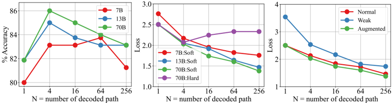
Automatic process annotation exhibits satisfactory quality. Figure 4(a) demonstrates that utilizing LLaMA2-70B trained on MetaMATH as the completer, the accuracy of the hard estimation (HE) reaches 86% when N equals 4. This suggests that our automatically constructed dataset is of high quality. However, we observed a decline in the accuracy of the constructed dataset with further increases in N. Our analysis indicates that larger values for N may lead to false positives.
Figure 4(b) shows the cross-entropy loss between SE and HE labels compared to the human-annotated distribution: as N increases, SE progressively aligns closer to the standard distribution, in contrast to HE which does not exhibit similar behavior. It is essential to note that at N=4, HE achieves an accuracy of 86%. We can theoretically attain higher quality data exceeding 86% accuracy by utilizing SE. However, we discovered that the performance of the verifier exhibits no substantial divergence whether trained with either SE or HE. This may be attributable to the already high-quality annotations provided by HE.
Furthermore, we also delve into other automatic process annotation methodologies. For instance, (Li et al., 2023b) employs a natural language inference (NLI) model and a string match rule to annotate a
Figure 3: Performance of LLaMA2-70B using different verification strategies across different numbers of solution candidates on GSM8K and MATH.
<details>
<summary>Image 5 Details</summary>
### Visual Description
\n
## Line Charts: GSM8K and MATH Benchmark Performance
### Overview
The image displays two side-by-side line charts comparing the performance of different methods on two mathematical reasoning benchmarks: GSM8K (left) and MATH (right). Both charts plot the percentage of problems solved against the number of solutions sampled per problem (N), using a "Best-of-N" evaluation metric. The charts demonstrate how performance scales with increased sampling for each method.
### Components/Axes
**Common Elements (Both Charts):**
* **X-Axis:** Labeled "N = number of solutions per problem". It uses a logarithmic scale with discrete markers at N = 1, 4, 16, 64, and 256.
* **Y-Axis:** Labeled "% Problems Solved (Best-of-N)". The scale is linear.
* **Legend:** Positioned in the bottom-right corner of each chart's plot area. It lists the methods with corresponding colored line and marker symbols.
* **Data Representation:** Each method is represented by a solid line connecting circular data points. A semi-transparent shaded band around each line likely indicates confidence intervals or variance.
**GSM8K Chart (Left):**
* **Title:** "GSM8K" (centered at the top).
* **Y-Axis Range:** Approximately 78% to 94%.
* **Legend Entries:**
* `SC` (Red line, red circle marker)
* `ORM` (Blue line, blue circle marker)
* `SHEPHERD` (Green line, green circle marker)
**MATH Chart (Right):**
* **Title:** "MATH" (centered at the top).
* **Y-Axis Range:** Approximately 28% to 45%.
* **Legend Entries:**
* `SC` (Red line, red circle marker)
* `ORM` (Blue line, blue circle marker)
* `PRM800K` (Purple line, purple circle marker)
* `SHEPHERD` (Green line, green circle marker)
### Detailed Analysis
**GSM8K Chart Data & Trends:**
* **Trend Verification:** All three lines show a clear upward trend that begins to plateau after N=64. The slope is steepest between N=1 and N=16.
* **Data Points (Approximate % Solved):**
* **N=1:** All methods start at nearly the same point, ~80.5%.
* **N=4:** SHEPHERD (Green) and ORM (Blue) rise sharply to ~88.5%. SC (Red) rises more slowly to ~83%.
* **N=16:** SHEPHERD leads at ~92%. ORM is close behind at ~91%. SC reaches ~86.5%.
* **N=64:** SHEPHERD ~93%. ORM ~92%. SC ~88%.
* **N=256:** SHEPHERD ~93.5%. ORM ~92%. SC ~88.2%. The gains from N=64 to N=256 are minimal for all methods.
**MATH Chart Data & Trends:**
* **Trend Verification:** All four lines show an upward trend that also begins to plateau, though the overall performance is significantly lower than on GSM8K. The initial slope (N=1 to N=16) is steep.
* **Data Points (Approximate % Solved):**
* **N=1:** All methods start clustered around 29%.
* **N=4:** SHEPHERD (Green) leads at ~36%. ORM (Blue) and PRM800K (Purple) are near ~35%. SC (Red) is lowest at ~33%.
* **N=16:** SHEPHERD ~41.5%. PRM800K ~39.5%. ORM ~39.5%. SC ~37%.
* **N=64:** SHEPHERD ~43.5%. PRM800K ~40.5%. ORM ~40%. SC ~38%.
* **N=256:** SHEPHERD ~44.5%. PRM800K ~41%. ORM ~40.5%. SC ~39.2%. The performance gap between SHEPHERD and the others widens slightly as N increases.
### Key Observations
1. **Consistent Hierarchy:** On both benchmarks, the `SHEPHERD` method (green) consistently achieves the highest performance at every value of N > 1. `SC` (red) consistently performs the worst.
2. **Dataset Difficulty:** The absolute performance on the MATH benchmark (y-axis max ~45%) is substantially lower than on GSM8K (y-axis max ~94%), indicating MATH is a more challenging dataset for all evaluated methods.
3. **Diminishing Returns:** For all methods on both tasks, the performance gain from increasing N shows clear diminishing returns. The most significant improvements occur when moving from N=1 to N=16. The curves flatten considerably between N=64 and N=256.
4. **Method Comparison:** `ORM` (blue) and `PRM800K` (purple, only on MATH) perform similarly, occupying a middle tier between SHEPHERD and SC. On MATH, PRM800K holds a very slight edge over ORM at higher N values.
5. **Starting Point Convergence:** At N=1 (single solution), all methods within each chart start at approximately the same performance level. The differentiation between methods emerges and grows as more solutions are sampled (N increases).
### Interpretation
The data suggests that the `SHEPHERD` method is more effective at leveraging increased sampling (higher N) to find correct solutions compared to `SC`, `ORM`, and `PRM800K`. Its superior scaling indicates it may have a better underlying strategy for generating or selecting among multiple candidate solutions.
The stark difference in overall scores between GSM8K and MATH highlights the increased complexity of the MATH dataset, which likely requires more advanced reasoning steps. The fact that all methods show similar scaling patterns (steep initial rise, then plateau) implies a fundamental limit to the "Best-of-N" sampling approach; simply generating more solutions yields progressively smaller benefits.
The close performance of `ORM` and `PRM800K` suggests these methods may share similar underlying mechanisms or limitations. The consistent underperformance of `SC` (likely "Self-Consistency") indicates that its approach to aggregating multiple solutions is less effective than the others tested in this evaluation setup.
**Language Declaration:** All text in the image is in English.
</details>
Figure 4: Quality of process annotation on GSM8K. (a): Accuracy of the process annotation using different completer; (b): Loss of the process annotation using different completer; (c): Loss of the process annotation using the same completer with different training data.
<details>
<summary>Image 6 Details</summary>
### Visual Description
\n
## Multi-Panel Line Chart Series: Performance Metrics vs. Decoded Paths
### Overview
The image contains three separate line charts arranged horizontally. Each chart plots a different performance metric (Accuracy, Loss, and another Loss metric) against the same independent variable: the number of decoded paths (`N`). The charts compare different model sizes (7B, 13B, 70B) and training conditions (Soft, Hard, Normal, Weak, Augmented). The overall purpose is to visualize how model performance scales with increased decoding paths under various configurations.
### Components/Axes
**Common Elements:**
* **X-Axis (All Charts):** Labeled `N = number of decoded path`. The scale is logarithmic, with major tick marks at 1, 4, 16, 64, and 256.
* **Legend Position:** All legends are located in the top-right corner of their respective chart panels.
**Chart 1 (Left): Accuracy**
* **Y-Axis:** Labeled `% Accuracy`. Scale ranges from 80 to 86, with major ticks at 80, 82, 84, 86.
* **Legend:**
* Red line with circle markers: `7B`
* Blue line with circle markers: `13B`
* Green line with circle markers: `70B`
**Chart 2 (Center): Loss (Model Size & Training Type)**
* **Y-Axis:** Labeled `Loss`. Scale ranges from 1.0 to 3.0, with major ticks at 1.0, 1.5, 2.0, 2.5, 3.0.
* **Legend:**
* Red line with circle markers: `7B:Soft`
* Blue line with circle markers: `13B:Soft`
* Green line with circle markers: `70B:Soft`
* Purple line with circle markers: `70B:Hard`
**Chart 3 (Right): Loss (Training Condition)**
* **Y-Axis:** Labeled `Loss`. Scale ranges from 1 to 4, with major ticks at 1, 2, 3, 4.
* **Legend:**
* Red line with circle markers: `Normal`
* Blue line with circle markers: `Weak`
* Green line with circle markers: `Augmented`
### Detailed Analysis
**Chart 1: Accuracy vs. N**
* **7B (Red Line):** Starts at ~80.0% (N=1). Increases to a peak of ~83.2% at N=4. Plateaus around 83.2% for N=16 and N=64. Decreases to ~81.2% at N=256.
* **13B (Blue Line):** Starts at ~81.8% (N=1). Sharp increase to a peak of ~85.0% at N=4. Decreases to ~83.8% at N=16, then to ~83.2% at N=64. Slight increase to ~83.4% at N=256.
* **70B (Green Line):** Starts at ~81.8% (N=1). Sharp increase to the highest peak on the chart, ~86.0%, at N=4. Decreases to ~85.0% at N=16, then to ~83.8% at N=64. Levels off at ~83.2% at N=256.
* **Trend Verification:** All three model sizes show an initial sharp improvement in accuracy from N=1 to N=4, followed by a general decline or plateau as N increases further. The 70B model achieves the highest peak accuracy.
**Chart 2: Loss vs. N (by Model & Training)**
* **7B:Soft (Red Line):** Starts highest at ~2.8 (N=1). Decreases steadily to ~2.1 (N=4), ~1.9 (N=16), ~1.8 (N=64), and ~1.75 (N=256).
* **13B:Soft (Blue Line):** Starts at ~2.5 (N=1). Decreases to ~2.0 (N=4), ~1.8 (N=16), ~1.6 (N=64), and ~1.5 (N=256).
* **70B:Soft (Green Line):** Starts at ~2.5 (N=1). Decreases to ~1.9 (N=4), ~1.7 (N=16), ~1.5 (N=64), and ~1.35 (N=256). This line shows the steepest and most consistent decline.
* **70B:Hard (Purple Line):** Starts at ~2.5 (N=1). Decreases to ~2.1 (N=4), then increases slightly to ~2.25 (N=16), ~2.3 (N=64), and ~2.3 (N=256). This is the only line that shows an increasing trend after N=4.
* **Trend Verification:** For the "Soft" training condition, loss decreases consistently as N increases, with larger models (70B) achieving lower final loss. The "Hard" training condition for the 70B model shows a different pattern, with loss bottoming out at N=4 and then rising.
**Chart 3: Loss vs. N (by Training Condition)**
* **Normal (Red Line):** Starts at ~2.5 (N=1). Decreases to ~2.0 (N=4), ~1.8 (N=16), ~1.6 (N=64), and ~1.4 (N=256).
* **Weak (Blue Line):** Starts highest at ~3.5 (N=1). Decreases to ~2.5 (N=4), ~2.1 (N=16), ~1.8 (N=64), and ~1.7 (N=256). It remains the highest loss line throughout.
* **Augmented (Green Line):** Starts at ~2.5 (N=1). Decreases to ~2.0 (N=4), ~1.7 (N=16), ~1.5 (N=64), and ~1.35 (N=256). It closely tracks and ends slightly lower than the "Normal" line.
* **Trend Verification:** All three training conditions show a consistent downward trend in loss as N increases. The "Weak" condition starts with significantly higher loss but improves at a similar rate. The "Augmented" condition yields the lowest final loss.
### Key Observations
1. **Peak at N=4:** Accuracy for all models peaks at N=4 before declining. This suggests an optimal point for accuracy with a small number of decoded paths.
2. **Model Scaling Benefit:** In the Accuracy chart, the 70B model achieves the highest peak. In the Loss chart (Soft training), the 70B model achieves the lowest final loss, demonstrating clear benefits from scaling model size.
3. **Training Condition Impact:** The "Hard" training condition for the 70B model (Chart 2, purple line) results in a fundamentally different loss trajectory compared to "Soft" training, with loss increasing after N=4. The "Weak" condition (Chart 3, blue line) starts with much higher loss but follows a similar improvement curve.
4. **Diminishing Returns:** After N=4, increasing the number of decoded paths yields diminishing returns for accuracy and, in most cases, continues to reduce loss but at a slower rate.
### Interpretation
The data suggests a complex relationship between model scale, training methodology, decoding effort (`N`), and performance. The consistent peak in accuracy at N=4 across model sizes indicates that a small amount of decoding diversity significantly helps, but beyond that, additional paths may introduce noise or overfitting to the decoding process, harming accuracy. However, loss continues to decrease (or stabilize) with more paths for most configurations, suggesting the model's confidence or calibration improves even if final accuracy does not.
The stark difference between the `70B:Soft` and `70B:Hard` lines is particularly notable. It implies that the "Hard" training regime may make the model's loss landscape such that exploring more decoding paths (higher N) becomes detrimental, possibly due to overconfidence or a sharper optimum. The "Augmented" training condition appears most effective for minimizing loss in the long run.
From a practical standpoint, these charts argue for tuning the number of decoded paths (`N`) as a critical hyperparameter. The optimal `N` is not simply "more is better"; it depends on the model size, the training method, and whether the primary goal is maximizing accuracy or minimizing loss. For accuracy-focused tasks, a small `N` (like 4) may be optimal, while for tasks where model confidence (loss) is key, a larger `N` could be beneficial, depending on the training setup.
</details>
given step. The NLI-based method annotates a step as correct if it is entailment with any step in the reference solutions. The Rule-based method annotates a step as correct if its support number precisely matches that of any steps in the reference solutions. As demonstrated in Table 4, our annotation strategy exhibits substantial superiority over the two approaches.
The ability of the LLM completer plays an important role in the data quality. We employ a completer to finalize multiple subsequent reasoning processes for a given step. Therefore, we investigate the impact of the LLM completer.
Figure 4(b) presents the cross-entropy loss across diverse completers trained on MetaMath. The results indicate that a larger completer is adept at generating superior-quality datasets. Figure 4(c) depicts the cross-entropy loss of LLaMA2-70B trained with different datasets. 'Normal' denotes the original GSM8K training dataset; 'Weak' refers to the Normal set excluding examples whose questions are in our 160 evaluation set; while 'Augmented' symbolizes MetaMath, an augmented version of the Normal set.
The findings suggest that high-quality training sets allow the model to operate more proficiently as a completer. Importantly, the 'Weak' set exhibits a markedly larger loss than other datasets. This insight drives us to infer that LLMs should acquire the questions in advance to enhance their performance as completers. We can also conjecture that a stronger foundational model, coupled with superior training data, could further enhance the quality of automatic annotation.
## 5.3 INFLUENCE OF THE PRE-TRAINED BASE MODELS
To conduct an exhaustive evaluation of MATH-SHEPHERD's effectiveness, we performed a diverse range of experiments using model sizes 7B, 13B, and 70B.
Table 4: The comparison between NLI/Rule-based automatic process annotation methods from Li et al. (2023b) and our method.
| Methods | Models | Accuracy (%) | Loss |
|---------------------------------|---------------------------|----------------|--------|
| DIVERSE-NLI (Li et al., 2023b) | DeBERTa (He et al., 2020) | 61.3 | 5.43 |
| DIVERSE-NLI (Li et al., 2023b) | LLaMA2-13B | 75.6 | 3.27 |
| DIVERSE-Rule (Li et al., 2023b) | - | 75 | 3.43 |
| MATH-SHEPHERD | LLaMA2-13B (N = 4) | 85 | 2.05 |
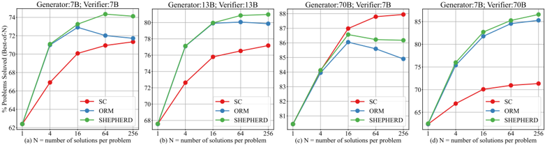
Figure 5: Performance of different verification strategies on different sizes of generators and verifiers.
<details>
<summary>Image 7 Details</summary>
### Visual Description
## Line Charts: Performance Scaling with Number of Solutions (N)
### Overview
The image contains four line charts arranged horizontally, labeled (a) through (d). Each chart plots the percentage of problems solved (y-axis) against the number of solutions per problem, N (x-axis, logarithmic scale). The charts compare the performance of three methods—SC, ORM, and SHEPHERD—across different configurations of Generator and Verifier model sizes (measured in billions of parameters, B).
### Components/Axes
* **Common Elements (All Charts):**
* **X-axis:** Label: `N = number of solutions per problem`. Scale: Logarithmic, with markers at `1`, `4`, `16`, `64`, `256`.
* **Y-axis:** Label: `% Problems Solved (Base=N)`. Scale: Linear, but the range varies per subplot.
* **Legend:** Located in the top-left corner of each subplot. Contains three entries:
* `SC` (Red line with circular markers)
* `ORM` (Blue line with circular markers)
* `SHEPHERD` (Green line with circular markers)
* **Subplot-Specific Titles (Top of each chart):**
* (a) `Generator:7B, Verifier:7B`
* (b) `Generator:13B, Verifier:13B`
* (c) `Generator:70B, Verifier:70B`
* (d) `Generator:7B, Verifier:70B`
### Detailed Analysis
**Chart (a): Generator:7B, Verifier:7B**
* **Y-axis Range:** 62% to 74%.
* **Data Series Trends & Approximate Points:**
* **SC (Red):** Shows a steady, concave-down increase. Starts lowest at N=1 (~62%), rises to ~70% at N=16, and ends at ~71.5% at N=256.
* **ORM (Blue):** Increases to a peak and then declines. Starts at ~62% (N=1), peaks at ~73% (N=16), then falls to ~71.5% (N=256).
* **SHEPHERD (Green):** Shows the steepest and most sustained increase. Starts at ~62% (N=1), surpasses ORM by N=64 (~73.5%), and reaches the highest value of ~74% at N=256.
**Chart (b): Generator:13B, Verifier:13B**
* **Y-axis Range:** 68% to 80%.
* **Data Series Trends & Approximate Points:**
* **SC (Red):** Steady increase. Starts at ~68% (N=1), reaches ~76% (N=16), and ends at ~77% (N=256).
* **ORM (Blue):** Increases to a peak and then declines. Starts at ~68% (N=1), peaks at ~79% (N=16), then falls to ~78% (N=256).
* **SHEPHERD (Green):** Strong, sustained increase. Starts at ~68% (N=1), matches ORM at N=16 (~79%), and continues rising to ~80% at N=256, becoming the top performer.
**Chart (c): Generator:70B, Verifier:70B**
* **Y-axis Range:** 80% to 88%.
* **Data Series Trends & Approximate Points:**
* **SC (Red):** Strong, steady increase. Starts at ~80% (N=1), rises to ~87% (N=16), and ends at ~88% (N=256).
* **ORM (Blue):** Increases to a peak and then declines. Starts at ~80% (N=1), peaks at ~86% (N=16), then falls to ~85% (N=256).
* **SHEPHERD (Green):** Increases and then plateaus. Starts at ~80% (N=1), rises to ~86.5% (N=16), and remains around ~86.5% through N=256.
**Chart (d): Generator:7B, Verifier:70B**
* **Y-axis Range:** 65% to 85%.
* **Data Series Trends & Approximate Points:**
* **SC (Red):** Increases and then plateaus. Starts at ~65% (N=1), rises to ~70% (N=16), and ends at ~71% (N=256).
* **ORM (Blue):** Shows a strong, sustained increase. Starts at ~65% (N=1), rises to ~82% (N=16), and continues to ~85% at N=256.
* **SHEPHERD (Green):** Shows the strongest, most sustained increase. Starts at ~65% (N=1), rises to ~83% (N=16), and reaches the highest value of ~86% at N=256.
### Key Observations
1. **SHEPHERD's Scaling:** The SHEPHERD method (green) consistently shows the most robust positive scaling with N across all configurations. It either becomes the top performer at high N (charts a, b, d) or maintains a high plateau (chart c).
2. **ORM's Peak and Decline:** The ORM method (blue) consistently peaks at N=16 in charts (a), (b), and (c), after which its performance declines as N increases to 64 and 256. This negative scaling at high N is a notable anomaly.
3. **Impact of Model Size:** Moving from 7B (a) to 13B (b) to 70B (c) models (matched generator/verifier) shifts the entire performance range upward (from ~62-74% to ~68-80% to ~80-88%).
4. **Verifier vs. Generator Size:** Chart (d) isolates the effect of a large verifier (70B) with a small generator (7B). Compared to chart (a) (both 7B), performance is dramatically higher (up to ~86% vs. ~74%), suggesting verifier size is a critical factor. In this configuration, both SHEPHERD and ORM scale very well with N, unlike SC which plateaus.
### Interpretation
This data demonstrates the relationship between inference-time compute (number of solutions, N) and problem-solving accuracy for different methods and model scales. The key finding is that the **SHEPHERD method is uniquely effective at converting additional compute (higher N) into improved accuracy**, showing positive scaling where other methods plateau or even decline.
The anomalous decline of ORM at high N in matched-size models (a, b, c) suggests a potential failure mode or inefficiency in its verification or aggregation process when overwhelmed with many candidate solutions. In contrast, the strong performance in chart (d) indicates that a powerful verifier can mitigate this issue, even with a weaker generator.
Overall, the charts argue that for maximizing the benefit of increased inference compute (scaling N), the choice of method (SHEPHERD) and the relative scale of the verifier model are more critical than simply scaling both generator and verifier together. The data provides a practical guide for resource allocation in AI problem-solving systems.
</details>
Figures 5(a), 5(b), and 3(a) display the results from the 7B, 13B, and 70B generators paired with equal-sized reward models, respectively. It becomes evident that PRM exhibits superiority over self-consistency and ORM across all sizes of base models. Moreover, bigger reward models prove to be more robust; for instance, the accuracy of the 70B reward models escalates as the number of candidate solutions rises, while the 7B reward models show a decreasing trend.
Figure 5(c) and 5(d) presents the performance of 7B and 70B generators interfaced with differentsized reward models. The findings illustrate that utilizing a larger reward model to validate the output of a smaller generator significantly enhances performance. Conversely, when a smaller reward model is employed to validate the output of a larger generator, the verification process adversely impacts the model's performance compared to SC. These results substantiate that we should utilize a more potent reward model for validating or supervising the generator.
## 5.4 INFLUENCE OF THE NUMBER OF DATA
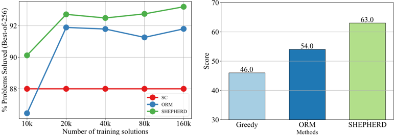
We delve deeper into the analysis of PRM and ORM by utilizing varying quantities of training data. As depicted in Figure 6(a), it is clear that PRM exhibits superior data efficiency. Specifically, it outperforms ORM by approximately 4% accuracy when applying a modestly sized training dataset (i.e., 10k instances). Furthermore, PRM seems to have a higher potential ceiling than ORM. These observations highlight the efficacy of PRM for verification purposes.
## 5.5 OUT-OF-DISTRIBUTION PERFORMANCE
To further demonstrate the effectiveness of our method, we conduct an out-of-distribution evaluation on the Hungarian national final exam 2 , which consists of 33 questions. The total score of these questions is 100. We use the LLemma-34B trained on MetaMATH to serve as the generator and generate 256 candidate solutions for each question. We use LLemma-34B-ORM and LLemma34B-PRM to select the solution for each question. As shown in Figure 6(b): 1) both LLemma34B-ORM and LLemma-34B-PRM outperform the origin LLemma-34B, showing the reward model can generalize to other domains; 2) PRM outperforms ORM 9 scores, further demonstrating the superiority of PRM.
2 https://huggingface.co/datasets/keirp/hungarian\_national\_hs\_finals\_ exam
Figure 6: (a): Performance of different reward models using different numbers of training data; (b) performance of different verification strategies on the out-of-distribution Hungarian national exam.
<details>
<summary>Image 8 Details</summary>
### Visual Description
## Line Chart and Bar Chart: Performance Comparison of Methods
### Overview
The image contains two distinct charts presented side-by-side. The left chart is a line graph comparing the performance of three methods (SC, ORM, SHEPHERD) as the number of training solutions increases. The right chart is a bar graph comparing the final scores of three methods (Greedy, ORM, SHEPHERD). All text in the image is in English.
### Components/Axes
**Left Chart (Line Graph):**
* **Y-axis:** Label: "% Problems Solved (Best-of-256)". Scale ranges from 88 to 92, with major gridlines at 88, 90, and 92.
* **X-axis:** Label: "Number of training solutions". Categories: 10k, 20k, 40k, 80k, 160k.
* **Legend:** Located in the bottom-right corner of the chart area. It defines three data series:
* Red line with circle markers: **SC**
* Blue line with circle markers: **ORM**
* Green line with circle markers: **SHEPHERD**
**Right Chart (Bar Graph):**
* **Y-axis:** Label: "Score". Scale ranges from 30 to 70, with major gridlines at 30, 40, 50, 60, and 70.
* **X-axis:** Label: "Methods". Categories: **Greedy**, **ORM**, **SHEPHERD**.
* **Bars:** Each bar is a solid color with its numerical value displayed on top.
* Greedy: Light blue bar.
* ORM: Dark blue bar.
* SHEPHERD: Light green bar.
### Detailed Analysis
**Left Chart - Line Graph Data Points & Trends:**
* **SC (Red Line):** The trend is perfectly flat. It starts at 88% at 10k solutions and remains constant at 88% for all subsequent points (20k, 40k, 80k, 160k).
* **ORM (Blue Line):** The trend shows a sharp initial increase followed by a slight decline and plateau.
* 10k: ~88.5%
* 20k: 92% (sharp increase)
* 40k: ~91.8% (slight decrease)
* 80k: ~91.5% (further slight decrease)
* 160k: ~91.8% (slight recovery)
* **SHEPHERD (Green Line):** The trend is generally upward with minor fluctuations, consistently performing the best.
* 10k: 90%
* 20k: ~92.5% (peak)
* 40k: ~92.2% (slight dip)
* 80k: ~92.5% (returns to peak level)
* 160k: ~93% (highest point)
**Right Chart - Bar Graph Data Points:**
* **Greedy:** Score = 46.0
* **ORM:** Score = 54.0
* **SHEPHERD:** Score = 63.0
### Key Observations
1. **Performance Hierarchy:** SHEPHERD is the top-performing method in both charts. It solves the highest percentage of problems and achieves the highest score.
2. **SC Stagnation:** The SC method shows no improvement whatsoever with increased training solutions, remaining fixed at 88%.
3. **ORM's Plateau:** ORM shows a significant performance jump when moving from 10k to 20k training solutions but then plateaus and even slightly regresses, never surpassing its 20k peak of 92%.
4. **SHEPHERD's Consistency:** SHEPHERD not only starts strong (90% at 10k) but also shows a general upward trend, reaching its highest performance at the maximum training solution count (160k).
5. **Score Correlation:** The bar chart confirms the superiority shown in the line chart. SHEPHERD's score (63.0) is 9 points higher than ORM (54.0) and 17 points higher than Greedy (46.0).
### Interpretation
The data suggests a clear conclusion about the efficacy of the tested methods. **SHEPHERD is demonstrably the most effective approach** among those compared, both in terms of the percentage of problems it can solve (a measure of capability or coverage) and its final score (a measure of quality or performance).
The line chart reveals an important dynamic: simply increasing the amount of training data (solutions) does not guarantee linear improvement. While SHEPHERD benefits from more data, ORM hits a point of diminishing returns very early (after 20k solutions), and SC is completely unresponsive to it. This implies that the SHEPHERD method has a superior architecture or learning algorithm that can effectively leverage additional data, whereas the other methods are fundamentally limited.
The bar chart provides a summary metric that aligns perfectly with the detailed trend analysis. The significant gaps between the bars (Greedy < ORM < SHEPHERD) indicate that the performance differences are substantial and not marginal. From a technical or research perspective, this evidence strongly advocates for the adoption or further development of the SHEPHERD method over the alternatives presented.
</details>
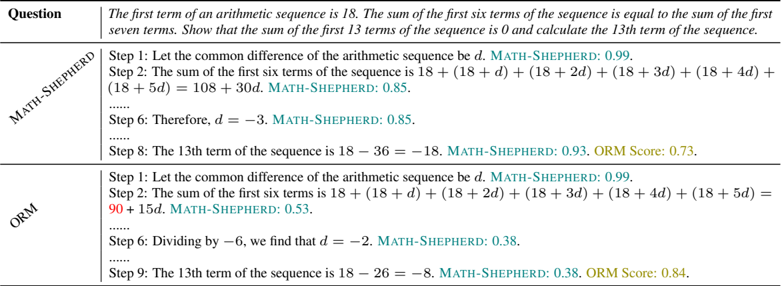
Table 5: A case study from the Hungarian national exam. Red text denotes the mistake that ORM fails to detect.
<details>
<summary>Image 9 Details</summary>
### Visual Description
\n
## Mathematical Solution Comparison: Arithmetic Sequence Problem
### Overview
The image displays a side-by-side comparison of two different solution methods (labeled "MATH-SHEPHERD" and "ORM") for the same arithmetic sequence problem. The problem statement is presented at the top, followed by the two solution approaches in a table-like format. Each solution shows selected steps, mathematical expressions, and associated scoring metrics.
### Components/Axes
* **Problem Statement (Top):** "The first term of an arithmetic sequence is 18. The sum of the first six terms of the sequence is equal to the sum of the first seven terms. Show that the sum of the first 13 terms of the sequence is 0 and calculate the 13th term of the sequence."
* **Solution Labels (Left Column, Rotated Text):**
* Top Row: "MATH-SHEPHERD"
* Bottom Row: "ORM"
* **Solution Steps (Right Column):** Each solution presents a series of numbered steps (e.g., Step 1, Step 2, Step 6, Step 8/9) with mathematical derivations. Ellipses ("......") indicate omitted intermediate steps.
* **Scoring Metrics:** Embedded within the steps are colored text annotations providing scores:
* `MATH-SHEPHERD: [value]` (in teal/cyan)
* `ORM Score: [value]` (in gold/yellow, appears only in the final step of the ORM solution)
### Detailed Analysis
**MATH-SHEPHERD Solution:**
* **Step 1:** "Let the common difference of the arithmetic sequence be *d*." Score: `MATH-SHEPHERD: 0.99`.
* **Step 2:** "The sum of the first six terms of the sequence is 18 + (18 + *d*) + (18 + 2*d*) + (18 + 3*d*) + (18 + 4*d*) + (18 + 5*d*) = 108 + 30*d*." Score: `MATH-SHEPHERD: 0.85`.
* **Step 6:** "Therefore, *d* = -3." Score: `MATH-SHEPHERD: 0.85`.
* **Step 8:** "The 13th term of the sequence is 18 - 36 = -18." Scores: `MATH-SHEPHERD: 0.93`, `ORM Score: 0.73`.
**ORM Solution:**
* **Step 1:** "Let the common difference of the arithmetic sequence be *d*." Score: `MATH-SHEPHERD: 0.99`.
* **Step 2:** "The sum of the first six terms of the sequence is 18 + (18 + *d*) + (18 + 2*d*) + (18 + 3*d*) + (18 + 4*d*) + (18 + 5*d*) = **90 + 15*d***." (The expression "90 + 15*d*" is highlighted in red). Score: `MATH-SHEPHERD: 0.53`.
* **Step 6:** "Dividing by -6, we find that *d* = -2." Score: `MATH-SHEPHERD: 0.38`.
* **Step 9:** "The 13th term of the sequence is 18 - 26 = -8." Scores: `MATH-SHEPHERD: 0.38`, `ORM Score: 0.84`.
### Key Observations
1. **Divergent Results:** The two methods yield different values for the common difference (*d* = -3 vs. *d* = -2) and consequently different answers for the 13th term (-18 vs. -8).
2. **Error Identification:** The MATH-SHEPHERD score for Step 2 of the ORM solution is notably low (0.53), and the resulting sum expression "90 + 15*d*" is highlighted in red, indicating an identified error in that calculation.
3. **Scoring Pattern:** The MATH-SHEPHERD scores generally decrease for the ORM solution as the error propagates through the steps (0.99 -> 0.53 -> 0.38 -> 0.38). The final ORM Score for its own solution is 0.84.
4. **Problem Requirements:** The problem asks to *show* the sum of the first 13 terms is 0. Neither solution explicitly shows this proof in the visible steps, focusing instead on finding *d* and the 13th term.
### Interpretation
This image is likely a diagnostic or evaluation output from an automated math-solving or tutoring system. It compares a correct or reference solution (MATH-SHEPHERD) against a student or alternative attempt (ORM).
* **What the data suggests:** The MATH-SHEPHERD solution appears to be the correct pathway. The error in the ORM solution's Step 2 (incorrect summation leading to 90 + 15*d* instead of 108 + 30*d*) is the root cause of its incorrect final answer. The scoring metrics (MATH-SHEPHERD scores) seem to assess the correctness or quality of each individual step, flagging the erroneous step with a low score.
* **Relationship between elements:** The side-by-side layout facilitates direct comparison of methodology and accuracy. The colored scores provide immediate, step-wise feedback. The red highlighting on the incorrect expression serves as a visual cue for the point of divergence.
* **Notable anomaly:** The final "ORM Score: 0.84" for the incorrect ORM solution is surprisingly high given the fundamental error. This might indicate the scoring system weights certain aspects (like problem setup or final answer format) heavily, or that the score is not purely a measure of mathematical correctness but perhaps of process or partial credit. This discrepancy between the low step-wise MATH-SHEPHERD scores and the higher final ORM Score is a key point for investigation into the scoring algorithm's design.
</details>
| Question | The first term of an arithmetic sequence is 18. The sum of the first six terms of the sequence is equal to the sum of the first seven terms. Show that the sum of the first 13 terms of the sequence is 0 and calculate the 13th term of the sequence. |
|---------------|------------------------------------------------------------------------------------------------------------------------------------------------------------------------------------------------------------------------------------------------------------------------------------------------------------------------------------------------------------------------------------------------------------------|
| MATH-SHEPHERD | Step 1: Let the common difference of the arithmetic sequence be d . MATH-SHEPHERD: 0.99. Step 2: The sum of the first six terms of the sequence is 18 +(18+ d ) +(18+2 d ) +(18+3 d ) +(18+4 d )+ (18+5 d ) = 108 +30 d . MATH-SHEPHERD: 0.85. ...... Step 6: Therefore, d = - 3 . MATH-SHEPHERD: 0.85. ...... Step 8: The 13th term of the sequence is 18 - 36 = - 18 . MATH-SHEPHERD: 0.93. ORMScore: 0.73. |
| ORM | Step 1: Let the common difference of the arithmetic sequence be d . MATH-SHEPHERD: 0.99. Step 2: The sum of the first six terms is 18 +(18+ d ) +(18+2 d ) +(18+3 d ) +(18+4 d ) +(18+5 d ) = 90 + 15 d . MATH-SHEPHERD: 0.53. ...... Step 6: Dividing by - 6 , we find that d = - 2 . MATH-SHEPHERD: 0.38. ...... Step 9: The 13th term of the sequence is 18 - 26 = - 8 . MATH-SHEPHERD: 0.38. ORMScore: 0.84. |
We also conduct a case study to intuitively demonstrate the effectiveness of MATH-SHEPHERD. As outlined in Table 5, when presented with a question from the Hungarian national final exam, our MATH-SHEPHERD accurately selected the correct solution from a pool of 256 potential solutions, which ORM failed. Moreover, MATH-SHEPHERD displayed superior discernment by precisely identifying incorrect steps within the solutions selected by ORM. Notably, it recognized errors in Step 2, Step 6, and Step 9 and so on, and subsequently assigned them lower scores relative to those for steps present in the correct solutions.
## 6 LIMITATIONS
Our paper has some limitations, which we leave for future work:
The computational cost of the completion process. To determine the label of each reasoning step, we utilize a 'completer' to decode N subsequent reasoning processes. We observe that as N increases, so does the quality of automatic annotations. However, this completion process demands a lot of computing resources, potentially imposing a limitation on the usage of our method. Despite this limitation, the cost remains significantly lower than human annotation. Furthermore, we are optimistic that advancements in efficient inference techniques such as speculative decoding (Xia et al., 2022; Leviathan et al., 2023) and vLLM (Kwon et al., 2023) could mitigate this limitation.
The automatic process annotation consists of noise. Similar to the automatic outcome annotation, our automatic process annotation also has noise. Despite this, our experiments verify the efficacy of our method for training a PRM. In particular, the PRM trained on our dataset outperforms the human-annotated PRM800K dataset. However, a noticeable gap remains between PRM800K and the candidate responses generated by the open-source models utilized in this study, which may result in the invalidation of PRM800K. As a result, the impact of this potential noise on PRM performance is still undetermined. A comprehensive comparison between human and automated annotations is envisaged for future studies. Furthermore, we assert that integrating human and automated process annotations could play a vital role in constructing robust and efficient process supervision.
## 7 CONCLUSION
In this paper, we introduce a process-oriented math verifier called MATH-SHEPHERD, which assigns a reward score to each step of the LLM's outputs on math problems. The training of MATH-SHEPHERD is achieved using automatically constructed process-wise supervision data, thereby eradicating the necessity for labor-intensive human annotation. Remarkably, this automatic methodology correlates strongly with human annotations. Extensive experiments in both verification and reinforcement learning scenarios demonstrate the effectiveness of our method.
## REFERENCES
- Rohan Anil, Andrew M Dai, Orhan Firat, Melvin Johnson, Dmitry Lepikhin, Alexandre Passos, Siamak Shakeri, Emanuel Taropa, Paige Bailey, Zhifeng Chen, et al. Palm 2 technical report. arXiv preprint arXiv:2305.10403 , 2023.
- Zhangir Azerbayev, Hailey Schoelkopf, Keiran Paster, Marco Dos Santos, Stephen McAleer, Albert Q Jiang, Jia Deng, Stella Biderman, and Sean Welleck. Llemma: An open language model for mathematics. arXiv preprint arXiv:2310.10631 , 2023.
- Zhen Bi, Ningyu Zhang, Yinuo Jiang, Shumin Deng, Guozhou Zheng, and Huajun Chen. When do program-of-thoughts work for reasoning? arXiv preprint arXiv:2308.15452 , 2023.
- S´ ebastien Bubeck, Varun Chandrasekaran, Ronen Eldan, Johannes Gehrke, Eric Horvitz, Ece Kamar, Peter Lee, Yin Tat Lee, Yuanzhi Li, Scott Lundberg, et al. Sparks of artificial general intelligence: Early experiments with gpt-4. arXiv preprint arXiv:2303.12712 , 2023.
- Liang Chen, Yichi Zhang, Shuhuai Ren, Haozhe Zhao, Zefan Cai, Yuchi Wang, Peiyi Wang, Tianyu Liu, and Baobao Chang. Towards end-to-end embodied decision making via multi-modal large language model: Explorations with gpt4-vision and beyond. arXiv preprint arXiv:2310.02071 , 2023.
- Karl Cobbe, Vineet Kosaraju, Mohammad Bavarian, Mark Chen, Heewoo Jun, Lukasz Kaiser, Matthias Plappert, Jerry Tworek, Jacob Hilton, Reiichiro Nakano, et al. Training verifiers to solve math word problems. arXiv preprint arXiv:2110.14168 , 2021.
- R´ emi Coulom. Efficient selectivity and backup operators in monte-carlo tree search. In International conference on computers and games , pp. 72-83. Springer, 2006.
- DeepSeek. Deepseek llm: Let there be answers. https://github.com/deepseek-ai/ DeepSeek-LLM , 2023.
- Yao Fu, Hao Peng, Ashish Sabharwal, Peter Clark, and Tushar Khot. Complexity-based prompting for multi-step reasoning. arXiv preprint arXiv:2210.00720 , 2022.
- Zhibin Gou, Zhihong Shao, Yeyun Gong, Yujiu Yang, Minlie Huang, Nan Duan, Weizhu Chen, et al. Tora: A tool-integrated reasoning agent for mathematical problem solving. arXiv preprint arXiv:2309.17452 , 2023.
- Pengcheng He, Xiaodong Liu, Jianfeng Gao, and Weizhu Chen. Deberta: Decoding-enhanced bert with disentangled attention. arXiv preprint arXiv:2006.03654 , 2020.
- Dan Hendrycks, Collin Burns, Saurav Kadavath, Akul Arora, Steven Basart, Eric Tang, Dawn Song, and Jacob Steinhardt. Measuring mathematical problem solving with the math dataset. arXiv preprint arXiv:2103.03874 , 2021.
- Jie Huang and Kevin Chen-Chuan Chang. Towards reasoning in large language models: A survey. In Anna Rogers, Jordan Boyd-Graber, and Naoaki Okazaki (eds.), Findings of the Association for Computational Linguistics: ACL 2023 , pp. 1049-1065, Toronto, Canada, July 2023. Association for Computational Linguistics. doi: 10.18653/v1/2023.findings-acl.67. URL https://aclanthology.org/2023.findings-acl.67 .
- Jie Huang, Xinyun Chen, Swaroop Mishra, Huaixiu Steven Zheng, Adams Wei Yu, Xinying Song, and Denny Zhou. Large language models cannot self-correct reasoning yet. arXiv preprint arXiv:2310.01798 , 2023.
- Albert Q Jiang, Alexandre Sablayrolles, Arthur Mensch, Chris Bamford, Devendra Singh Chaplot, Diego de las Casas, Florian Bressand, Gianna Lengyel, Guillaume Lample, Lucile Saulnier, et al. Mistral 7b. arXiv preprint arXiv:2310.06825 , 2023.
- Jean Kaddour, Joshua Harris, Maximilian Mozes, Herbie Bradley, Roberta Raileanu, and Robert McHardy. Challenges and applications of large language models. arXiv preprint arXiv:2307.10169 , 2023.
- Levente Kocsis and Csaba Szepesv´ ari. Bandit based monte-carlo planning. In European conference on machine learning , pp. 282-293. Springer, 2006.
- Woosuk Kwon, Zhuohan Li, Siyuan Zhuang, Ying Sheng, Lianmin Zheng, Cody Hao Yu, Joseph Gonzalez, Hao Zhang, and Ion Stoica. Efficient memory management for large language model serving with pagedattention. In Proceedings of the 29th Symposium on Operating Systems Principles , pp. 611-626, 2023.
- Yaniv Leviathan, Matan Kalman, and Yossi Matias. Fast inference from transformers via speculative decoding. In International Conference on Machine Learning , pp. 19274-19286. PMLR, 2023.
- Lei Li, Yuwei Yin, Shicheng Li, Liang Chen, Peiyi Wang, Shuhuai Ren, Mukai Li, Yazheng Yang, Jingjing Xu, Xu Sun, et al. M3it: A large-scale dataset towards multi-modal multilingual instruction tuning. arXiv preprint arXiv:2306.04387 , 2023a.
- Yifei Li, Zeqi Lin, Shizhuo Zhang, Qiang Fu, Bei Chen, Jian-Guang Lou, and Weizhu Chen. Making language models better reasoners with step-aware verifier. In Anna Rogers, Jordan BoydGraber, and Naoaki Okazaki (eds.), Proceedings of the 61st Annual Meeting of the Association for Computational Linguistics (Volume 1: Long Papers) , pp. 5315-5333, Toronto, Canada, July 2023b. Association for Computational Linguistics. doi: 10.18653/v1/2023.acl-long.291. URL https://aclanthology.org/2023.acl-long.291 .
- Hunter Lightman, Vineet Kosaraju, Yura Burda, Harri Edwards, Bowen Baker, Teddy Lee, Jan Leike, John Schulman, Ilya Sutskever, and Karl Cobbe. Let's verify step by step. arXiv preprint arXiv:2305.20050 , 2023.
- Haipeng Luo, Qingfeng Sun, Can Xu, Pu Zhao, Jianguang Lou, Chongyang Tao, Xiubo Geng, Qingwei Lin, Shifeng Chen, and Dongmei Zhang. Wizardmath: Empowering mathematical reasoning for large language models via reinforced evol-instruct. arXiv preprint arXiv:2308.09583 , 2023.
- Qianli Ma, Haotian Zhou, Tingkai Liu, Jianbo Yuan, Pengfei Liu, Yang You, and Hongxia Yang. Let's reward step by step: Step-level reward model as the navigators for reasoning. arXiv preprint arXiv:2310.10080 , 2023.
- OpenAI. GPT-4 technical report. CoRR , abs/2303.08774, 2023. doi: 10.48550/arXiv.2303.08774. URL https://doi.org/10.48550/arXiv.2303.08774 .
- Sarah Pan, Vladislav Lialin, Sherin Muckatira, and Anna Rumshisky. Let's reinforce step by step. arXiv preprint arXiv:2311.05821 , 2023.
- Joon Sung Park, Joseph O'Brien, Carrie Jun Cai, Meredith Ringel Morris, Percy Liang, and Michael S Bernstein. Generative agents: Interactive simulacra of human behavior. In Proceedings of the 36th Annual ACM Symposium on User Interface Software and Technology , pp. 1-22, 2023.
- David Silver, Aja Huang, Chris J Maddison, Arthur Guez, Laurent Sifre, George Van Den Driessche, Julian Schrittwieser, Ioannis Antonoglou, Veda Panneershelvam, Marc Lanctot, et al. Mastering the game of go with deep neural networks and tree search. nature , 529(7587):484-489, 2016.
- Yifan Song, Weimin Xiong, Dawei Zhu, Cheng Li, Ke Wang, Ye Tian, and Sujian Li. Restgpt: Connecting large language models with real-world applications via restful apis. corr, abs/2306.06624, 2023. doi: 10.48550. arXiv preprint arXiv.2306.06624 .
- Maciej ´ Swiechowski, Konrad Godlewski, Bartosz Sawicki, and Jacek Ma´ ndziuk. Monte carlo tree search: A review of recent modifications and applications. Artificial Intelligence Review , 56(3): 2497-2562, 2023.
- Hugo Touvron, Louis Martin, Kevin Stone, Peter Albert, Amjad Almahairi, Yasmine Babaei, Nikolay Bashlykov, Soumya Batra, Prajjwal Bhargava, Shruti Bhosale, et al. Llama 2: Open foundation and fine-tuned chat models. arXiv preprint arXiv:2307.09288 , 2023.
- Jonathan Uesato, Nate Kushman, Ramana Kumar, Francis Song, Noah Siegel, Lisa Wang, Antonia Creswell, Geoffrey Irving, and Irina Higgins. Solving math word problems with process-and outcome-based feedback. arXiv preprint arXiv:2211.14275 , 2022.
- Guanzhi Wang, Yuqi Xie, Yunfan Jiang, Ajay Mandlekar, Chaowei Xiao, Yuke Zhu, Linxi Fan, and Anima Anandkumar. Voyager: An open-ended embodied agent with large language models. arXiv preprint arXiv:2305.16291 , 2023a.
- Peiyi Wang, Lei Li, Liang Chen, Feifan Song, Binghuai Lin, Yunbo Cao, Tianyu Liu, and Zhifang Sui. Making large language models better reasoners with alignment. arXiv preprint arXiv:2309.02144 , 2023b.
- Peiyi Wang, Lei Li, Liang Chen, Dawei Zhu, Binghuai Lin, Yunbo Cao, Qi Liu, Tianyu Liu, and Zhifang Sui. Large language models are not fair evaluators. arXiv preprint arXiv:2305.17926 , 2023c.
- Xuezhi Wang, Jason Wei, Dale Schuurmans, Quoc V. Le, Ed H. Chi, Sharan Narang, Aakanksha Chowdhery, and Denny Zhou. Self-consistency improves chain of thought reasoning in language models. In The Eleventh International Conference on Learning Representations, ICLR 2023, Kigali, Rwanda, May 1-5, 2023 . OpenReview.net, 2023d. URL https://openreview.net/ pdf?id=1PL1NIMMrw .
- Jason Wei, Xuezhi Wang, Dale Schuurmans, Maarten Bosma, Brian Ichter, Fei Xia, Ed H. Chi, Quoc V. Le, and Denny Zhou. Chain-of-thought prompting elicits reasoning in large language models. In NeurIPS , 2022. URL http://papers.nips.cc/paper\_files/paper/2022/hash/ 9d5609613524ecf4f15af0f7b31abca4-Abstract-Conference.html .
- Zeqiu Wu, Yushi Hu, Weijia Shi, Nouha Dziri, Alane Suhr, Prithviraj Ammanabrolu, Noah A Smith, Mari Ostendorf, and Hannaneh Hajishirzi. Fine-grained human feedback gives better rewards for language model training. arXiv preprint arXiv:2306.01693 , 2023.
- Heming Xia, Tao Ge, Furu Wei, and Zhifang Sui. Lossless speedup of autoregressive translation with generalized aggressive decoding. arXiv preprint arXiv:2203.16487 , 2022.
- Fei Yu, Anningzhe Gao, and Benyou Wang. Outcome-supervised verifiers for planning in mathematical reasoning. arXiv preprint arXiv:2311.09724 , 2023a.
- Longhui Yu, Weisen Jiang, Han Shi, Jincheng Yu, Zhengying Liu, Yu Zhang, James T Kwok, Zhenguo Li, Adrian Weller, and Weiyang Liu. Metamath: Bootstrap your own mathematical questions for large language models. arXiv preprint arXiv:2309.12284 , 2023b.
- Zheng Yuan, Hongyi Yuan, Chengpeng Li, Guanting Dong, Chuanqi Tan, and Chang Zhou. Scaling relationship on learning mathematical reasoning with large language models. arXiv preprint arXiv:2308.01825 , 2023.
- Xiang Yue, Xingwei Qu, Ge Zhang, Yao Fu, Wenhao Huang, Huan Sun, Yu Su, and Wenhu Chen. Mammoth: Building math generalist models through hybrid instruction tuning. arXiv preprint arXiv:2309.05653 , 2023.
- Yifan Zhang, Jingqin Yang, Yang Yuan, and Andrew Chi-Chih Yao. Cumulative reasoning with large language models. arXiv preprint arXiv:2308.04371 , 2023.
- Lianmin Zheng, Wei-Lin Chiang, Ying Sheng, Siyuan Zhuang, Zhanghao Wu, Yonghao Zhuang, Zi Lin, Zhuohan Li, Dacheng Li, Eric Xing, et al. Judging llm-as-a-judge with mt-bench and chatbot arena. arXiv preprint arXiv:2306.05685 , 2023.
- Xinyu Zhu, Junjie Wang, Lin Zhang, Yuxiang Zhang, Yongfeng Huang, Ruyi Gan, Jiaxing Zhang, and Yujiu Yang. Solving math word problems via cooperative reasoning induced language models. In Anna Rogers, Jordan Boyd-Graber, and Naoaki Okazaki (eds.), Proceedings of the 61st Annual Meeting of the Association for Computational Linguistics (Volume 1: Long Papers) , pp. 4471-4485, Toronto, Canada, July 2023. Association for Computational Linguistics. doi: 10.18653/v1/2023. acl-long.245. URL https://aclanthology.org/2023.acl-long.245 .