2401.10020

# Self-Rewarding Language Models Abstract We posit that to achieve superhuman agents, future models require superhuman feedback in order to provide an adequate training signal. Current approaches commonly train reward models from human preferences, which may then be bottlenecked by human performance level, and secondly these separate frozen reward models cannot then learn to improve during LLM training. In this work, we study Self-Rewarding Language Models, where the language model itself is used via LLM-as-a-Judge prompting to provide its own rewards during training. We show that during Iterative DPO training that not only does instruction following ability improve, but also the ability to provide high-quality rewards to itself. Fine-tuning Llama 2 70B on three iterations of our approach yields a model that outperforms many existing systems on the AlpacaEval 2.0 leaderboard, including Claude 2, Gemini Pro, and GPT-4 0613. While there is much left still to explore, this work opens the door to the possibility of models that can continually improve in both axes. 1 Introduction Aligning Large Language Models (LLMs) using human preference data can vastly improve the instruction following performance of pretrained models (Ouyang et al., 2022; Bai et al., 2022a). The standard approach of Reinforcement Learning from Human Feedback (RLHF) learns a reward model from these human preferences. The reward model is then frozen and used to train the LLM using RL, e.g., via PPO (Schulman et al., 2017). A recent alternative is to avoid training the reward model at all, and directly use human preferences to train the LLM, as in Direct Preference Optimization (DPO; Rafailov et al., 2023). In both cases, the approach is bottlenecked by the size and quality of the human preference data, and in the case of RLHF the quality of the frozen reward model trained from them as well. In this work, we instead propose to train a self-improving reward model that, rather than being frozen, is continually updating during LLM alignment, in order to avoid this bottleneck. The key to such an approach is to develop an agent that possesses all the abilities desired during training, rather than separating them out into distinct models such as a reward model and a language model. In the same way that pretraining and multitasking training of instruction following tasks allow task transfer by training on many tasks at once (Collobert and Weston, 2008; Radford et al., 2019; Ouyang et al., 2022), incorporating the reward model into that same system allows task transfer between the reward modeling task and the instruction following tasks. 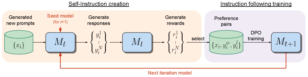We thus introduce Self-Rewarding Language Models, that both (i) act as instruction following models generating responses for given prompts; and (ii) can generate and evaluate new instruction following examples to add to their own training set. We train these models using an Iterative DPO framework similar to that recently introduced in Xu et al. (2023). Starting from a seed model, in each iteration there is a process of Self-Instruction creation whereby candidate responses are generated by the model for newly created prompts, and are then assigned rewards by that same model. The latter is implemented via LLM-as-a-Judge prompting, which can also be seen as an instruction following task. A preference dataset is built from the generated data, and the next iteration of the model is trained via DPO, see Figure 1. In our experiments, we start with a Llama 2 70B (Touvron et al., 2023) seed model fine-tuned on Open Assistant (Köpf et al., 2023), and then perform the above training scheme. We find that not only does the instruction following performance improve from Self-Rewarding LLM alignment compared to the baseline seed model, but importantly the reward modeling ability, which is no longer fixed, improves as well. This means that the model during iterative training is able, at a given iteration, to provide a higher quality preference dataset to itself than in the previous iteration. While this effect likely saturates in real-world settings, it provides the intriguing possibility of obtaining reward models (and hence LLMs) that are superior to ones that could have been trained from the original human-authored seed data alone. 2 Self-Rewarding Language Models Our approach first assumes access to a base pretrained language model, and a small amount of human-annotated seed data. We then build a model that aims to possess two skills simultaneously: 1. Instruction following: given a prompt that describes a user request, the ability to generate a high quality, helpful (and harmless) response. 1. Self-Instruction creation: the ability to generate and evaluate new instruction-following examples to add to its own training set. These skills are used so that the model can perform self-alignment, i.e., they are the components used to iteratively train itself using AI Feedback (AIF). Self-instruction creation consists of generating candidate responses and then the model itself judging their quality, i.e., it acts as its own reward model, replacing the need for an external one. This is implemented via the LLM-as-a-Judge mechanism (Zheng et al., 2023b), i.e., by formulating the evaluation of responses as an instruction following task. This self-created AIF preference data is used as a training set. <details> <summary>x1.png Details</summary>  ### Visual Description \n ## Diagram: Self-Instruction Creation and Instruction Following Training ### Overview This diagram illustrates a two-stage process: Self-Instruction creation and Instruction Following training, used to iteratively improve a model (Mt). The process begins with generating new prompts, proceeds through response and reward generation, and culminates in training a new model iteration (Mt+1). A feedback loop connects the final model to the initial prompt generation stage. ### Components/Axes The diagram is divided into two main sections, visually separated by a light gray background: "Self-Instruction creation" (left) and "Instruction following training" (right). Key components within these sections are represented as labeled boxes and processes. * **Generated new prompts:** Represented by a cylinder labeled "{xᵢ}". * **Seed model (for t-1):** Represented by a rectangle labeled "Mₜ". * **Generate responses:** Represented by a curly brace labeled "{y₁ / y₂ / ... / yN}". * **Generate rewards:** Represented by a curly brace labeled "{r₁ / r₂ / ... / rN}". * **Preference pairs:** Represented by a cylinder labeled "{xᵢ, y₁ , y₂}". * **DPO training:** Text label "DPO training". * **Next iteration model:** Text label "Next iteration model" with a red arrow connecting the two sections. * **Next iteration model (Mt+1):** Represented by a rectangle labeled "Mₜ₊₁". * **Select:** Text label "select". ### Detailed Analysis / Content Details The diagram depicts a sequential flow of information. 1. **Self-Instruction Creation:** * New prompts "{xᵢ}" are fed into the seed model "Mₜ". * The model generates responses "{y₁ / y₂ / ... / yN}". * These responses are then used to generate rewards "{r₁ / r₂ / ... / rN}". * A selection process chooses preference pairs "{xᵢ, y₁ , y₂}". 2. **Instruction Following Training:** * The selected preference pairs are used for DPO (Direct Preference Optimization) training. * This training results in the next iteration model "Mₜ₊₁". 3. **Feedback Loop:** * A red arrow labeled "Next iteration model" indicates that the new model "Mₜ₊₁" is used as the seed model for the next iteration of prompt generation, creating a continuous improvement cycle. ### Key Observations The diagram highlights an iterative process of self-improvement. The use of preference pairs and DPO training suggests a reinforcement learning approach. The feedback loop is crucial for refining the model's ability to follow instructions. The notation of t-1 and t+1 indicates a time-series or iterative process. ### Interpretation This diagram illustrates a method for improving language models through self-generated training data. The model learns by creating its own prompts, evaluating its responses, and then using this feedback to refine its parameters. This approach is particularly valuable when labeled training data is scarce or expensive to obtain. The DPO training step suggests a focus on aligning the model's behavior with human preferences. The iterative nature of the process allows the model to continuously improve its performance over time. The diagram doesn't provide specific data or numerical values, but rather a conceptual overview of the training pipeline. It suggests a system designed for autonomous learning and refinement of instruction-following capabilities in a language model. </details> Figure 1: Self-Rewarding Language Models. Our self-alignment method consists of two steps: (i) Self-Instruction creation: newly created prompts are used to generate candidate responses from model $M_{t}$ , which also predicts its own rewards via LLM-as-a-Judge prompting. (ii) Instruction following training: preference pairs are selected from the generated data, which are used for training via DPO, resulting in model $M_{t+1}$ . This whole procedure can then be iterated resulting in both improved instruction following and reward modeling ability. Our overall self-alignment procedure is an iterative one, which proceeds by building a series of such models, with the aim that each improves over the last. Importantly, because the model can both improve its generation ability, and act as its own reward model through the same generation mechanism, this means the reward model itself can improve through these iterations, deviating from standard practices where the reward model is fixed (Ouyang et al., 2022). We believe this can increase the ceiling of the potential for self-improvement of these learning models going forward, removing a constraining bottleneck. We describe these steps in more detail below. An overview of the approach is illustrated in Figure 1. 2.1 Initialization Seed instruction following data We are given a seed set of human-authored (instruction prompt, response) general instruction following examples that we use for training in a supervised fine-tuning (SFT) manner, starting from a pretrained base language model. Subsequently this will be referred to as Instruction Fine-Tuning (IFT) data. Seed LLM-as-a-Judge instruction following data We also assume we are provided a seed set of (evaluation instruction prompt, evaluation result response) examples which can also be used for training. While this is not strictly necessary, as the model using IFT data will already be capable of training an LLM-as-a-Judge, we show that such training data can give improved performance (see Appendix A.3 for supporting results). In this data, the input prompt asks the model to evaluate the quality of a given response to a particular instruction. The provided evaluation result response consists of chain-of-thought reasoning (a justification), followed by a final score (in our experiments out of 5). The exact prompt format we chose is given in Figure 2, which instructs the LLM to evaluate the response using five additive criteria (relevance, coverage, usefulness, clarity and expertise), covering various aspects of quality. Subsequently this will be referred to as Evaluation Fine-Tuning (EFT) data. We use both these seed sets together during training. 2.2 Self-Instruction Creation Using the model we have trained, we can make it self-modify its own training set. Specifically, we generate additional training data for the next iteration of training. This consists of the following steps: 1. Generate a new prompt: We generate a new prompt $x_{i}$ using few-shot prompting, sampling prompts from the original seed IFT data, following the approach of Wang et al. (2023) and Honovich et al. (2023). In our main experiments, responses and rewards, items (2) and (3), are generated by the model we have trained, but generating prompts is actually done by a model fixed in advance. However, we show that prompts can also be generated by the newly trained model in each iteration in Appendix A.5. 1. Generate candidate responses: We then generate $N$ diverse candidate responses $\{y_{i}^{1},...,y_{i}^{N}\}$ for the given prompt $x_{i}$ from our model using sampling. 1. Evaluate candidate responses: Finally, we use the LLM-as-a-Judge ability of our same model to evaluate its own candidate responses with scores $r_{i}^{n}∈[0,5]$ (exact prompt given in Figure 2). 2.3 Instruction Following Training As previously described, training is initially performed with the seed IFT and EFT data (Section 2.1). This is then augmented with additional data via AI (Self-)Feedback. AI Feedback Training After performing the self-instruction creation procedure, we can augment the seed data with additional examples for training, which we refer to as AI Feedback Training (AIFT) data. To do this, we construct preference pairs, which are training data of the form (instruction prompt $x_{i}$ , winning response $y_{i}^{w}$ , losing response $y_{i}^{l}$ ). To form the winning and losing pair we take the highest and lowest scoring responses from the $N$ evaluated candidate responses (see Section 2.2), following Xu et al. (2023), discarding the pair if their scores are the same. These pairs can be used for training with a preference tuning algorithm. We use DPO (Rafailov et al., 2023). Review the user’s question and the corresponding response using the additive 5-point scoring system described below. Points are accumulated based on the satisfaction of each criterion: - Add 1 point if the response is relevant and provides some information related to the user’s inquiry, even if it is incomplete or contains some irrelevant content. - Add another point if the response addresses a substantial portion of the user’s question, but does not completely resolve the query or provide a direct answer. - Award a third point if the response answers the basic elements of the user’s question in a useful way, regardless of whether it seems to have been written by an AI Assistant or if it has elements typically found in blogs or search results. - Grant a fourth point if the response is clearly written from an AI Assistant’s perspective, addressing the user’s question directly and comprehensively, and is well-organized and helpful, even if there is slight room for improvement in clarity, conciseness or focus. - Bestow a fifth point for a response that is impeccably tailored to the user’s question by an AI Assistant, without extraneous information, reflecting expert knowledge, and demonstrating a high-quality, engaging, and insightful answer. User: <INSTRUCTION_HERE> <response> <RESPONSE_HERE> </response> After examining the user’s instruction and the response: - Briefly justify your total score, up to 100 words. - Conclude with the score using the format: “Score: <total points>” Remember to assess from the AI Assistant perspective, utilizing web search knowledge as necessary. To evaluate the response in alignment with this additive scoring model, we’ll systematically attribute points based on the outlined criteria. Figure 2: LLM-as-a-Judge prompt for our LLM to act as a reward model and provide self-rewards for its own model generations. The model is initially trained with seed training data of how to perform well at this task, and then improves at this task further through our self-rewarding training procedure. 2.4 Overall Self-Alignment Algorithm Iterative Training Our overall procedure trains a series of models $M_{1},...,M_{T}$ where each successive model $t$ uses augmented training data created by the $t-1^{\text{th}}$ model. We thus define AIFT( $M_{t}$ ) to mean AI Feedback Training data created using model $M_{t}$ . Model Sequence We define the models, and the training data they use as follows: - : Base pretrained LLM with no fine-tuning. - : Initialized with $M_{0}$ , then fine-tuned on the IFT+EFT seed data using SFT. - : Initialized with $M_{1}$ , then trained with AIFT( $M_{1}$ ) data using DPO. - : Initialized with $M_{2}$ , then trained with AIFT( $M_{2}$ ) data using DPO. This iterative training resembles the procedure used in Pairwise Cringe Optimization and specifically is termed Iterative DPO, introduced in Xu et al. (2023); however, an external fixed reward model was used in that work. 3 Experiments 3.1 Experimental Setup Base Model In our experiments we use Llama 2 70B (Touvron et al., 2023) as our base pretrained model. 3.1.1 Seed Training Data IFT Seed Data We use the human-authored examples provided in the Open Assistant dataset (Köpf et al., 2023) for instruction fine-tuning. Following Li et al. (2024) we use 3200 examples, by sampling only first conversational turns in the English language that are high-quality, based on their human annotated rank (choosing only the highest rank 0). In our experiments, we compare to a model fine-tuned from the base model using only this data via supervised fine-tuning, and refer to it as our SFT baseline. EFT Seed Data The Open Assistant data also provides multiple ranked human responses per prompt from which we can construct evaluation fine-tuning data. We split this into train and evaluation sets, and use it to create LLM-as-a-Judge data. This is done by placing it in the input format given in Figure 2, which consists of the scoring criteria description, and the given instruction and response to be evaluated. Note, the prompt, derived from Li et al. (2024), mentions “utilizing web search”, but our model is not actually capable of this action. For training targets, chain-of-thought justifications and final scores out of 5 are not directly provided, so we use the SFT baseline to generate such output evaluations for each input, and accept them into the training set if the ranking of their scores agrees with the human rankings in the dataset. We resample the training set by discarding some of the data that receives the most common score so that the scores are not too skewed, as we observe many samples receive a score of 4. This results in 1,630 train and 541 evaluation examples (which do not overlap with the IFT data). 3.1.2 Evaluation Metrics We evaluate the performance of our self-rewarding models in two axes: their ability to follow instructions, and their ability as a reward model (ability to evaluate responses). Instruction Following We evaluate head-to-head performance between various models using GPT-4 (Achiam et al., 2023) as an evaluator over 256 test prompts (which we refer to as IFT test data) derived from various sources following Li et al. (2024) using the AlpacaEval evaluation prompt (Li et al., 2023). We try the prompt in both orders comparing pairwise, and if the GPT-4 evaluations disagree we count the result as a tie. We also perform a similar evaluation with humans (authors). We additionally report results in the AlpacaEval 2.0 leaderboard format which is evaluated over 805 prompts, and compute the win rate against the baseline GPT-4 Turbo model based on GPT-4 judgments. Further, we report results on MT-Bench (Zheng et al., 2023b) a set of challenging multi-turn questions in various categories from math and coding to roleplay and writing, which uses GPT-4 to grade the model responses out of 10. Finally we also test the models on a set of 9 NLP benchmarks: ARC-Easy (Clark et al., 2018), ARC-Challenge (Clark et al., 2018), HellaSwag (Zellers et al., 2019), SIQA (Sap et al., 2019), PIQA (Bisk et al., 2020), GSM8K (Cobbe et al., 2021), MMLU (Hendrycks et al., 2021), OBQA (Mihaylov et al., 2018) and NQ (Kwiatkowski et al., 2019). Reward Modeling We evaluate the correlation with human rankings on the evaluation set we derived from the Open Assistant dataset, as described in Section 3.1.1. Each instruction has on average 2.85 responses with given rankings. We can thus measure the pairwise accuracy, which is how many times the order of the ranking between any given pair agrees between the model’s evaluation and the human ranking. We also measure the exact match count, which is how often the total ordering is exactly the same for an instruction. We also report the Spearman correlation and Kendall’s $\tau$ . Finally, we report how often the responses that the model scores a perfect 5 out of 5 are rated as the highest ranked by humans. 3.1.3 Training Details Instruction following training The training hyperparameters we use are as follows. For SFT we use learning rate $5.5e{-6}$ which decays (cosine) to $1.1e{-6}$ at the end of training, batch size $16$ and dropout $0.1$ . We only calculate the loss on target tokens instead of the full sequence. For DPO we use learning rate $1e{-6}$ which decays to $1e{-7}$ , batch size $16$ , dropout $0.1$ , and a $\beta$ value of 0.1. We perform early stopping by saving a checkpoint every 200 steps and evaluating generations using Claude 2 (Anthropic, 2023) on 253 validation examples derived from various sources following Li et al. (2024). This is evaluated pairwise against the previous step’s generations using the AlpacaEval evaluation prompt format (Li et al., 2023). Self-Instruction creation To generate new prompts we use a fixed model, Llama 2-Chat 70B with 8-shot prompting following Self-Instruct (Wang et al., 2023), where we sample six demonstrations from the IFT data and two from the model generated data, and use decoding parameters T = 0.6, p = 0.9. We use their prompt template for non-classification tasks and apply the same filtering techniques, including the ROUGE-L (Lin, 2004) similarity check, keyword filtering, and length filtering. Except for the prompt generation part, the other parts of the creation pipeline (generating the response, and evaluating it) use the Self-Rewarding model being trained. For candidate response generation we sample $N=4$ candidate responses with temperature $T=0.7$ , $p=0.9$ . When evaluating candidate responses, as there is variance to these scores, in our experiments we also use sampled decoding (with the same parameters) and generate these evaluations multiple (3) times and take the average. We added 3,964 such preference pairs to form the AIFT( $M_{1}$ ) dataset used to train $M_{2}$ via DPO, and 6,942 pairs to form AIFT( $M_{2}$ ) used to train $M_{3}$ . 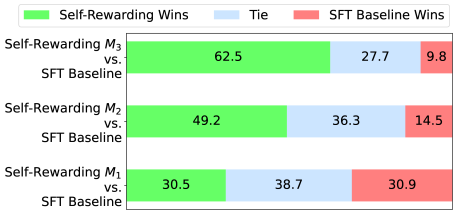3.2 Results 3.2.1 Instruction Following Ability Head to head performance results are provided in Figure 3. <details> <summary>x2.png Details</summary>  ### Visual Description \n ## Bar Chart: Self-Rewarding vs. SFT Baseline Wins ### Overview This is a horizontal stacked bar chart comparing the win rates of "Self-Rewarding" models (M1, M2, M3) against an "SFT Baseline" model. The chart displays the percentage of wins for each model, categorized into "Self-Rewarding Wins" (green), "Tie" (blue), and "SFT Baseline Wins" (red). ### Components/Axes * **Y-axis:** Lists the models being compared: "Self-Rewarding M3 vs. SFT Baseline", "Self-Rewarding M2 vs. SFT Baseline", and "Self-Rewarding M1 vs. SFT Baseline". * **X-axis:** Represents the percentage of wins, ranging from 0% to 100% (though the chart doesn't explicitly show these values, they are implied). * **Legend (Top-Left):** * Green: "Self-Rewarding Wins" * Blue: "Tie" * Red: "SFT Baseline Wins" ### Detailed Analysis The chart consists of three horizontal stacked bars, one for each Self-Rewarding model. Each bar is divided into three segments representing the win percentages for each category. * **Self-Rewarding M3 vs. SFT Baseline:** * Self-Rewarding Wins (Green): 62.5% * Tie (Blue): 27.7% * SFT Baseline Wins (Red): 9.8% * **Self-Rewarding M2 vs. SFT Baseline:** * Self-Rewarding Wins (Green): 49.2% * Tie (Blue): 36.3% * SFT Baseline Wins (Red): 14.5% * **Self-Rewarding M1 vs. SFT Baseline:** * Self-Rewarding Wins (Green): 30.5% * Tie (Blue): 38.7% * SFT Baseline Wins (Red): 30.9% ### Key Observations * The Self-Rewarding models generally outperform the SFT Baseline, but the degree of outperformance varies significantly. * M3 demonstrates the strongest performance, with a clear majority of wins (62.5%). * As the model number decreases (M3 to M2 to M1), the percentage of Self-Rewarding wins decreases, and the percentage of SFT Baseline wins increases. * The "Tie" percentage is relatively consistent across all three models, hovering around 30-40%. ### Interpretation The data suggests that the Self-Rewarding approach is effective in improving win rates compared to the SFT Baseline, but the effectiveness is dependent on the specific model (M1, M2, M3). Model M3 appears to benefit the most from the self-rewarding mechanism, while M1 shows a more marginal improvement. The consistent presence of ties indicates that a significant portion of the comparisons result in neither model clearly outperforming the other. The trend of decreasing Self-Rewarding wins and increasing SFT Baseline wins as the model number decreases suggests a potential correlation between the model architecture or training process and the effectiveness of the self-rewarding technique. Further investigation would be needed to understand the underlying reasons for this trend. The data implies that the self-rewarding mechanism is not universally beneficial and may require careful tuning or adaptation depending on the specific model being used. </details> <details> <summary>x3.png Details</summary>  ### Visual Description \n ## Stacked Bar Chart: Self-Rewarding Strategy Comparisons ### Overview This is a stacked horizontal bar chart comparing the win rates of different self-rewarding strategies (M3 vs. M2, M2 vs. M1, and M3 vs. M1). The chart displays the percentage of wins for the "Left" side, "Ties", and "Right" side for each strategy comparison. ### Components/Axes * **Y-axis:** Lists the strategy comparisons: "Self-Rewarding M3 vs. M2", "Self-Rewarding M2 vs. M1", and "Self-Rewarding M3 vs. M1". * **X-axis:** Represents the percentage of wins, ranging from approximately 0% to 70%. No explicit scale is provided, but the values suggest a linear scale. * **Legend (Top-Left):** * Green: "Left Wins (in Left vs. Right)" * Light Blue: "Tie" * Red: "Right Wins" ### Detailed Analysis The chart consists of three stacked horizontal bars, one for each strategy comparison. Each bar is divided into three segments representing the percentage of Left Wins, Ties, and Right Wins. 1. **Self-Rewarding M3 vs. M2:** * Left Wins (Green): 47.7% * Tie (Light Blue): 39.8% * Right Wins (Red): 12.5% 2. **Self-Rewarding M2 vs. M1:** * Left Wins (Green): 55.5% * Tie (Light Blue): 32.8% * Right Wins (Red): 11.7% 3. **Self-Rewarding M3 vs. M1:** * Left Wins (Green): 68.8% * Tie (Light Blue): 22.7% * Right Wins (Red): 8.6% ### Key Observations * The "Left Wins" percentage increases as the strategy comparison moves down the chart (M3 vs. M2 < M2 vs. M1 < M3 vs. M1). * The "Right Wins" percentage decreases as the strategy comparison moves down the chart. * The "Tie" percentage is relatively stable, fluctuating between 22.7% and 39.8%. * M3 vs. M1 has the highest Left Win rate (68.8%) and the lowest Right Win rate (8.6%). ### Interpretation The data suggests that the self-rewarding strategy M3 consistently outperforms M2 and M1, particularly when compared directly to M1. The increasing "Left Wins" and decreasing "Right Wins" percentages indicate a clear advantage for M3 in these scenarios. The relatively consistent "Tie" rate suggests that the overall level of uncertainty or equal performance remains similar across the different strategy comparisons. The chart demonstrates a hierarchical relationship between the strategies, with M3 appearing to be the most effective, followed by M2, and then M1. The differences in win rates are substantial enough to suggest that the choice of strategy has a significant impact on the outcome. </details> Figure 3: Instruction following ability improves with Self-Training: We evaluate our models using head-to-head win rates on diverse prompts using GPT-4. The SFT Baseline is on par with Self-Rewarding Iteration 1 ( $M_{1}$ ). However, Iteration 2 ( $M_{2}$ ) outperforms both Iteration 1 ( $M_{1}$ ) and the SFT Baseline. Iteration 3 ( $M_{3}$ ) gives further gains over Iteration 2 ( $M_{2}$ ), outperforming $M_{1}$ , $M_{2}$ and the SFT Baseline by a large margin. EFT+IFT seed training performs similarly to IFT alone We find that adding the Evaluation Fine-Tuning (EFT) task to training does not impact instruction following performance compared to using Instruction Fine-Tuning (IFT) data alone with an almost equal head to head (30.5% wins vs. 30.9% wins). This is a positive result because it means the increased capability of a model to self-reward does not affect its other skills. We can thus use IFT+EFT training as Iteration 1 ( $M_{1}$ ) of our Self-Rewarding model, and then run further iterations. Iteration 2 ( $M_{2}$ ) improves over Iteration 1 ( $M_{1}$ ) and SFT Baseline Iteration 2 of Self-Rewarding training ( $M_{2}$ ) provides superior instruction following to Iteration 1 ( $M_{1}$ ) with 55.5% wins for $M_{2}$ compared to only 11.7% for $M_{1}$ in a head to head evaluation. It provides similar gains over the SFT Baseline as well (49.2% wins vs. 14.5% wins). Clearly, there is a large jump in performance from $M_{1}$ to $M_{2}$ by using the preference data AIFT( $M_{1}$ ) provided by the reward model from Iteration 1. Iteration 3 ( $M_{3}$ ) improves over Iteration 2 ( $M_{2}$ ) We see a further gain in Iteration 3 over Iteration 2, with 47.7% wins for $M_{3}$ compared to only 12.5% for $M_{2}$ in a head to head evaluation. Similarly, the win rate over the SFT Baseline for $M_{3}$ increases to 62.5% wins vs. 9.8%, i.e., winning more often than the $M_{2}$ model did. Overall, we see large gains from $M_{2}$ to $M_{3}$ through training using the preference data AIFT( $M_{2}$ ) provided by the reward model from Iteration 2. Self-Rewarding models perform well on AlpacaEval 2 leaderboard We evaluate our models on the AlpacaEval 2.0 leaderboard format, with results given in Table 1. We observe the same findings as in the head-to-head evaluations, that training iterations yield improved win rates, in this case over GPT4-Turbo, from 9.94% in Iteration 1, to 15.38% in Iteration 2, to 20.44% in Iteration 3. Our Iteration 3 model outperforms many existing models in this metric, including Claude 2, Gemini Pro, and GPT4 0613. We show some selected models from the leaderboard in the table. We note that many of those competing models contain either proprietary alignment data (which is typically large, e.g., over 1M annotations in Touvron et al. (2023)) or use targets that are distilled from stronger models. In contrast, our Self-Rewarding model starts from a small set of seed data from Open Assistant, and then generates targets and rewards from the model itself for further iterations of training. Table 1: AlpacaEval 2.0 results (win rate over GPT-4 Turbo evaluated by GPT-4). Self-Rewarding iterations yield improving win rates. Iteration 3 ( $M_{3}$ ) outperforms many existing models that use proprietary training data or targets distilled from stronger models. | | | Alignment Targets | | | --- | --- | --- | --- | | Model | Win Rate | Distilled | Proprietary | | Self-Rewarding 70B | | | | | Iteration 1 ( $M_{1}$ ) | 9.94% | | | | Iteration 2 ( $M_{2}$ ) | 15.38% | | | | Iteration 3 ( $M_{3}$ ) | 20.44% | | | | Selected models from the leaderboard | | | | | GPT-4 0314 | 22.07% | | ✓ | | Mistral Medium | 21.86% | | ✓ | | Claude 2 | 17.19% | | ✓ | | Gemini Pro | 16.85% | | ✓ | | GPT-4 0613 | 15.76% | | ✓ | | GPT 3.5 Turbo 0613 | 14.13% | | ✓ | | LLaMA2 Chat 70B | 13.87% | | ✓ | | Vicuna 33B v1.3 | 12.71% | ✓ | | | Humpback LLaMa2 70B | 10.12% | | | | Guanaco 65B | 6.86% | | | | Davinci001 | 2.76% | | ✓ | | Alpaca 7B | 2.59% | ✓ | | <details> <summary>x4.png Details</summary>  ### Visual Description \n ## Line Chart: Win Rate by Category ### Overview This image presents a line chart illustrating the win rate (in percentage) across various categories. Four distinct data series, labeled M₀, M₁, M₂, and M₃, are plotted against a categorical x-axis representing different fields of interest. The chart aims to compare the win rates of these series across these categories. ### Components/Axes * **X-axis:** Categories - Health, Professional, Linguistics, Other, Entertainment, Technology, Literature, Coding, Science, Gaming, Philosophy, Social Studies, Travel, Arts, Sports, Mathematics, Social Interaction, DIY Projects, Cooking. * **Y-axis:** Win Rate (%) - Scale ranges from approximately 0% to 35%. * **Legend:** Located in the top-right corner. * M₀ (Dark Blue) * M₁ (Red) * M₂ (Orange) * M₃ (Light Orange) ### Detailed Analysis The chart displays the win rate for each category and each model (M₀, M₁, M₂, M₃). * **M₀ (Dark Blue):** This line generally fluctuates between approximately 5% and 25%. It starts at around 17% for Health, dips to approximately 8% for Professional, rises to around 22% for Linguistics, then decreases to around 10% for Other. It then rises to a peak of approximately 25% for Entertainment, drops to around 5% for Coding, and then fluctuates between 5% and 15% for the remaining categories, ending at approximately 7% for Cooking. * **M₁ (Red):** This line exhibits a more dramatic fluctuation. It begins at approximately 15% for Health, rises sharply to a peak of around 30% for Professional, then declines rapidly to approximately 0% for Coding. It then rises again to around 10% for Philosophy, and then fluctuates between 0% and 10% for the remaining categories, ending at approximately 2% for Cooking. * **M₂ (Orange):** This line shows a relatively stable trend, generally staying between approximately 20% and 30%. It starts at around 28% for Health, decreases to approximately 22% for Professional, then remains relatively stable around 25% for Linguistics, Other, Entertainment, and Technology. It then declines to around 20% for Literature, Coding, and Science, and then remains relatively stable around 18% to 22% for the remaining categories, ending at approximately 18% for Cooking. * **M₃ (Light Orange):** This line starts at approximately 25% for Health, decreases to around 20% for Professional, then remains relatively stable around 22% to 25% for Linguistics, Other, Entertainment, Technology, Literature, Coding, Science, Gaming, Philosophy, Social Studies, Travel, Arts, Sports, Mathematics, Social Interaction, and DIY Projects, ending at approximately 20% for Cooking. **Approximate Data Points (Read from the chart):** | Category | M₀ (%) | M₁ (%) | M₂ (%) | M₃ (%) | |-------------------|--------|--------|--------|--------| | Health | 17 | 15 | 28 | 25 | | Professional | 8 | 30 | 22 | 20 | | Linguistics | 22 | 20 | 25 | 23 | | Other | 10 | 18 | 25 | 24 | | Entertainment | 25 | 15 | 25 | 24 | | Technology | 22 | 12 | 25 | 24 | | Literature | 15 | 10 | 20 | 22 | | Coding | 5 | 0 | 20 | 22 | | Science | 10 | 5 | 18 | 21 | | Gaming | 8 | 8 | 20 | 21 | | Philosophy | 12 | 10 | 18 | 20 | | Social Studies | 15 | 8 | 18 | 20 | | Travel | 14 | 10 | 18 | 20 | | Arts | 10 | 8 | 18 | 19 | | Sports | 12 | 8 | 18 | 19 | | Mathematics | 10 | 8 | 18 | 19 | | Social Interaction| 8 | 5 | 18 | 18 | | DIY Projects | 10 | 5 | 18 | 18 | | Cooking | 7 | 2 | 18 | 20 | ### Key Observations * M₁ exhibits the most volatile win rate, with significant peaks and troughs. * M₂ and M₃ demonstrate relatively stable win rates across most categories. * M₀ shows moderate fluctuations, generally staying within a narrower range than M₁. * The highest win rates for M₁ are observed in the "Professional" category. * The lowest win rates for M₁ are observed in the "Coding" category. * The win rates for M₂ and M₃ are consistently higher than those of M₀ and M₁ across most categories. ### Interpretation The chart suggests that the performance of the models (M₀, M₁, M₂, M₃) varies significantly depending on the category. Model M₁ appears to be highly specialized, excelling in "Professional" fields but performing poorly in "Coding." Models M₂ and M₃ demonstrate more consistent performance across all categories, indicating a broader range of capabilities. The differences in win rates between the models could be attributed to variations in their training data, algorithms, or underlying architectures. The chart highlights the importance of considering category-specific performance when evaluating and selecting models for different tasks. The consistent performance of M₂ and M₃ might make them preferable for applications requiring reliable performance across a wide range of domains, while M₁ could be a valuable asset in specialized areas like "Professional" fields. The data suggests that the models are not universally superior in all areas, and their effectiveness is contingent upon the specific context. 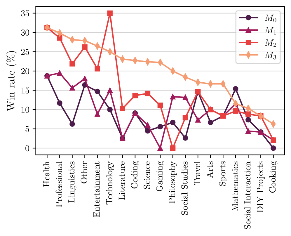</details> Figure 4: AlpacaEval win rate breakdown for instruction categories (full names given in Appendix). Self-Rewarding models give gains across several topics, but tend to e.g. give less gains on mathematics and reasoning tasks. Fine-grained analysis As described earlier, the overall performance of the model in AlpacaEval improves with each iteration of training. It would be interesting to break down the overall performance improvement to see exactly what type of tasks these improvements come from. Therefore, we cluster the instructions in AlpacaEval test set into different groups based on three perspectives: (1) instruction category (2) instruction complexity (3) expected response length. We achieve this by using GPT-4. The detailed statistical information of the breakdown and the prompting techniques we used for getting this breakdown can be found in Appendix A.6. Results for the instruction category are given in Figure 4, and the other two in Appendix Figure 11. From the results we can conclude that (i) Self-Rewarding models can substantially improve the win rate in most categories, but there are some tasks for which this approach does not improve, such as mathematics and logical reasoning, indicating that our current training approach mainly allows the models to better utilize their existing knowledge. (ii) Through Self-Rewarding model training, the model’s win rate increases on almost all tasks of different complexity, and especially on slightly more difficult tasks (complexity of 5, 6, 7 out of 10). (iii) The models also show a steady increase in the win rate on tasks with instructions with different expected response lengths. 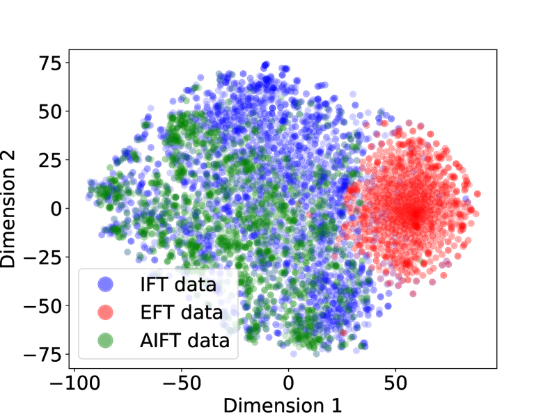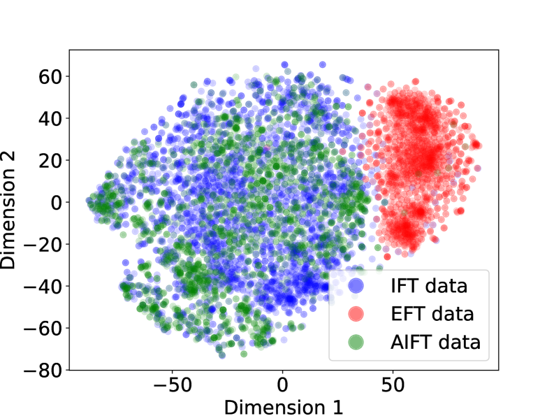Data distribution analysis We perform a t-SNE (Van der Maaten and Hinton, 2008) visualization of the IFT, EFT and AIFT( $M_{1}$ ) data, shown in Appendix A.1. We find good overlap between the IFT and AIFT( $M_{1}$ ) examples, which is desired, while the EFT examples lie in a different part of the embedding space, which can help explain why they would not affect IFT performance. We observe that generations from $M_{1}$ on AlpacaEval have an average length of 1092, for $M_{2}$ they are 1552, and for $M_{3}$ they are 2552, so the model is learning to generate longer responses, which we note may be a factor in relative performance. <details> <summary>x5.png Details</summary>  ### Visual Description \n ## Stacked Bar Chart: Self-Rewarding vs. SFT Baseline Wins ### Overview This is a stacked horizontal bar chart comparing the win rates of three "Self-Rewarding" models (M1, M2, and M3) against an "SFT Baseline" model. The chart displays the percentage of wins for each category: Self-Rewarding Wins (green), Ties (blue), and SFT Baseline Wins (red). ### Components/Axes * **Y-axis:** Lists the three model comparisons: "Self-Rewarding M3 vs. SFT Baseline", "Self-Rewarding M2 vs. SFT Baseline", and "Self-Rewarding M1 vs. SFT Baseline". * **X-axis:** Represents the percentage of wins, ranging from 0% to 100% (though the chart only displays up to 66%). No explicit axis label is present, but it is implied. * **Legend (Top-Left):** * Green: "Self-Rewarding Wins" * Blue: "Tie" * Red: "SFT Baseline Wins" ### Detailed Analysis The chart consists of three stacked bars, one for each model comparison. Each bar is divided into three segments representing the win percentages for each category. * **Self-Rewarding M3 vs. SFT Baseline:** * Self-Rewarding Wins (Green): Approximately 66.0% * Tie (Blue): Approximately 16.0% * SFT Baseline Wins (Red): Approximately 18.0% * **Self-Rewarding M2 vs. SFT Baseline:** * Self-Rewarding Wins (Green): Approximately 56.0% * Tie (Blue): Approximately 24.0% * SFT Baseline Wins (Red): Approximately 20.0% * **Self-Rewarding M1 vs. SFT Baseline:** * Self-Rewarding Wins (Green): Approximately 28.0% * Tie (Blue): Approximately 26.0% * SFT Baseline Wins (Red): Approximately 46.0% ### Key Observations * Self-Rewarding M3 consistently outperforms the SFT Baseline, with the highest percentage of wins (66.0%). * As the model number decreases (M3 to M2 to M1), the percentage of Self-Rewarding Wins decreases, and the percentage of SFT Baseline Wins increases. * The "Tie" percentage remains relatively stable across all three model comparisons, fluctuating between 16.0% and 26.0%. * Self-Rewarding M1 performs worse than the SFT Baseline, with only 28.0% wins compared to 46.0% for the baseline. ### Interpretation The data suggests that the self-rewarding mechanism is most effective in model M3, and its effectiveness diminishes as the model number decreases. Model M3 demonstrates a clear advantage over the SFT Baseline, while model M1 is outperformed by the baseline. The consistent presence of ties indicates that a significant portion of the comparisons result in neither model clearly winning. This could be due to the inherent complexity of the task or limitations in the evaluation metric. The trend suggests that the self-rewarding approach needs further refinement to consistently outperform the SFT Baseline across all models. The differences in performance between the models (M1, M2, M3) could be due to variations in their architecture, training data, or hyperparameter settings. Further investigation is needed to understand the factors contributing to these performance differences. 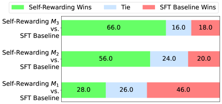</details> Figure 5: Human evaluation results. Iterations of Self-Rewarding ( $M_{1}$ , $M_{2}$ and $M_{3}$ ) provide progressively better head-to-head win rates compared to the SFT baseline, in agreement with the automatic evaluation results. Table 2: MT-Bench Results (on a scale of 10). Self-Rewarding iterations yield improving scores across various categories. Math, code & reasoning performance and iteration gains are smaller than for other categories, likely due to the makeup of the Open Assistant seed data we use. | $M_{1}$ $M_{2}$ $M_{3}$ | 6.78 7.01 7.25 | 3.83 4.05 4.17 | 8.55 8.79 9.10 | | --- | --- | --- | --- | Table 3: NLP Benchmarks. Self-Rewarding models mostly tend to maintain performance compared to the Llama 2 70B base model and the SFT Baseline, despite being fine-tuned on very different instruction-following prompts. | Llama 2 SFT Baseline $M_{1}$ | 57.40 55.97 57.51 | 85.30 85.17 84.99 | 56.80 50.72 60.27 | 68.90 69.76 69.34 | 25.30 34.35 35.48 | | --- | --- | --- | --- | --- | --- | | $M_{2}$ | 54.51 | 84.27 | 59.29 | 69.31 | 33.07 | | $M_{3}$ | 53.13 | 83.29 | 57.70 | 69.37 | 31.86 | Human evaluation To examine whether human judgments align with automatic evaluation results, we conduct human evaluations that compare SFT baseline generations with the generations from each iteration of Self-Rewarding training, i.e., models $M_{1}$ , $M_{2}$ , and $M_{3}$ . Specifically, we randomly select 50 instructions from the IFT test set. Each instruction corresponds to three pairs of generations (i.e., baseline vs. $M_{1}$ , baseline vs. $M_{2}$ , baseline vs. $M_{3}$ ). For each pair of generations, we assign them to three different annotators (blind evaluation performed by the authors) to make a pairwise judgment, and take a majority vote to decide which generation is better. The human evaluation results are shown in Figure 5. We find that Self-Rewarding models from later iterations show a larger advantage over the SFT baseline model, which is consistent with GPT-4’s judgments, and demonstrates the effectiveness of our iterative training procedure. MT-Bench performance further validates these results We report performance on MT-Bench in Table 2 for the SFT baseline and iterations of the Self-Rewarding model. We again see improvements across the iterations of training from $M_{1}$ to $M_{3}$ , from 6.78 (out of 10) up to 7.25, with larger relative gains in the humanities, STEM, roleplay, writing and extraction categories, and smaller gains in the math, code and reasoning categories. We expect that the latter is due to the seed prompts we use from Open Assistant tending to underemphasize the reasoning-based tasks. We note also that these improvements are in spite of our method using and constructing prompts that only involve a single turn, given the MT-Bench benchmark itself is a multi-turn evaluation. Self-rewarding models did not lose ability on NLP Benchmarks As shown in Table 3, the performance of most NLP benchmark tasks evaluated are roughly similar to the baselines, with further detailed results on more datasets given in Appendix Table 9 that follow the same pattern. We hypothesize that given that our training data (seed data and synthetically generated data) are based on the Open Assistant prompts which may not be especially relevant to skills needed in the Table 3 tasks, it is expected that the task performance stays roughly similar, or may even drop. For example, in InstructGPT training (Ouyang et al., 2022) they found that “during RLHF fine-tuning, we observe performance regressions compared to GPT-3 on certain public NLP datasets” which they refer to as an “alignment tax.” A clear future direction is to extend the self-rewarding paradigm to these types of tasks, by relying not only on seed prompts from Open Assistant, but also on seed prompts found in a larger variety of datasets. 3.2.2 Reward Modeling Ability Reward modeling evaluation results are provided in Table 4. EFT augmentation improves over SFT baseline Firstly, we find that adding Evaluation Fine-Tuning (EFT) data into training, which gives examples to the model of how to act as an LLM-as-a-Judge, naturally improves its performance compared to training with Instruction Fine-Tuning (IFT) data alone. IFT data covers a wide range of general instruction tasks, and so does endow the SFT Baseline with the ability to evaluate responses; however, EFT data gives more examples of this specific task. We find improvements across all five metrics measured when using IFT+EFT vs. IFT alone, e.g., the pairwise accuracy agreement with humans increases from 65.1% to 78.7%. Table 4: Reward Modeling ability improves with Self-Training: We evaluate the LLM-as-a-Judge via various metrics which measure alignment with held-out human preference data. Self-Rewarding Iteration 2 (Model $M_{2}$ ), which is trained using the self-reward model derived from its previous iteration $M_{1}$ outperforms Iteration 1 ( $M_{1}$ ), while $M_{1}$ itself outperforms a standard SFT baseline model trained on only Instruction Fine-Tuning (IFT) data. Iteration 3 (Model $M_{3}$ ) gives further improvements over Iteration 2. | Model Training data | SFT Baseline IFT | Self-Rewarding Models Iter 1 ( $M_{1}$ ) IFT+EFT | Iter 2 ( $M_{2}$ ) IFT+EFT | Iter 3 ( $M_{3}$ ) IFT+EFT+AIFT( $M_{1}$ ) | | --- | --- | --- | --- | --- | | +AIFT( $M_{1}$ ) | +AIFT( $M_{2}$ ) | | | | | Pairwise acc. $(\uparrow)$ | 65.1% | 78.7% | 80.4% | 81.7% | | 5-best % $(\uparrow)$ | 39.6% | 41.5% | 44.3% | 43.2% | | Exact Match % $(\uparrow)$ | 10.1% | 13.1% | 14.3% | 14.3% | | Spearman corr. $(\uparrow)$ | 0.253 | 0.279 | 0.331 | 0.349 | | Kendall $\tau$ corr. $(\uparrow)$ | 0.233 | 0.253 | 0.315 | 0.324 | Reward Modeling ability improves with Self-Training We find that performing a round of self-reward training improves the ability of the model at providing self-rewards for the next iteration, in addition to its improved instruction following ability. Model $M_{2}$ (Iteration 2) is trained using the reward model from $M_{1}$ (Iteration 1), but provides improved performance on all five metrics compared to $M_{1}$ . For example, pairwise accuracy improves from 78.7% to 80.4%. Iteration 3 ( $M_{3}$ ) improves several of these metrics further compared to $M_{2}$ , for example pairwise accuracy increases from 80.4% to 81.7%. This performance gain is achieved despite there being no additional EFT data provided, and the examples created during the Self-Instruction creation loop do not tend to look like LLM-as-a-Judge training examples. We hypothesize that because the model is becoming better at general instruction following, it nevertheless also improves at the LLM-as-a-Judge task. Importance of the LLM-as-a-Judge Prompt In these experiments we used the LLM-as-a-Judge prompt format shown in Figure 2. In preliminary experiments we also tried various other prompts to decide the most effective one to use. For example, we tried the prompt proposed in Li et al. (2024) which also proposes a 5-point scale, but describes the options as multiple choice in a range of quality buckets, see Appendix Figure 7. In contrast, our prompt describes the points as additive, covering various aspects of quality. We find a large difference between these two prompts when using the SFT Baseline, e.g. 65.1% pairwise accuracy for ours, and only 26.6% pairwise accuracy for theirs. See Appendix A.2 for further details. 4 Related Work Automatically improving or self-correcting large language models is becoming a major focus of research. A recent survey from Pan et al. (2023) attempts to summarize the topic. However, this is a rapidly moving area, and there are already promising new works not covered there. Reinforcement Learning from Human Feedback (RLHF) Preference learning approaches such as in Ziegler et al. (2019); Stiennon et al. (2020); Ouyang et al. (2022); Bai et al. (2022a) train a fixed reward model from human preference data, and then use the reward model to train via reinforcement learning (RL), e.g. via Proximal Policy Optimization (PPO) (Schulman et al., 2017). Thus, the reward signal in a certain sense already comes from a model even in these works, but distilled from human data. Nevertheless, this is commonly referred to as RL from Human Feedback (RLHF). Methods such as Direct Preference Optimization (DPO) (Rafailov et al., 2023) avoid training the reward model entirely, and instead directly train the LLM using human preferences. Several other such competing methods exist as well (Zhao et al., 2023; Zheng et al., 2023a; Yuan et al., 2023), including Pairwise Cringe Optimization (PCO) (Xu et al., 2023). PCO uses an iterative training approach similar to the one in our work, except with a fixed reward model, and that work also showed that Iterative DPO improves over DPO using the same scheme. We note that other works have developed iterative preference training schemes as well, e.g. Adolphs et al. (2023); Gulcehre et al. (2023); Xiong et al. (2023). Reinforcement Learning from AI Feedback (RLAIF) Constitutional AI (Bai et al., 2022b) uses an LLM to give feedback and refine responses, and uses this data to train a reward model. This fixed, separate reward model is then used to train the language model via RL, called “RL from AI Feedback” (RLAIF). Lee et al. (2023) compare RLAIF and RLHF procedures and find the methods they compare perform roughly equally. They use an “off-the-shelf” LLM to perform LLM-as-a-Judge prompting to build a training set to train a fixed reward model, which is then used for RL training. They also experiment with using the fixed but separate LLM-as-a-Judge model directly, which the authors report is computationally expensive due to using it within PPO training (rather than the offline step in the iterative approach we use in our work, which is relatively computationally cheap). Finally, SPIN (Chen et al., 2024b) recently showed they can avoid reward models entirely in an Iterative DPO-like framework by using human labels as the winning response in a pair, and the last iteration’s generations as the losing response in the pair. The authors note this has the limitation that once the model generations reach human performance, they are bottlenecked. Further, each input prompt is required to have a human annotated response, in contrast to our work. Improving LLMs via data augmentation (and curation) Several methods have improved LLMs by (self-)creating training data to augment fine-tuning. Self-Instruct (Wang et al., 2023) is a method for self-instruction creation of prompts and responses, which can be used to improve a base LLM. We make use of a similar technique in our work, and then use our self-reward model to score them. Several approaches have also created training data by distilling from powerful LLMs, and shown a weaker LLM can then perform well. For example, Alpaca (Taori et al., 2023) fine-tuned a Llama 7B model with text-davinci-003 instructions created in the style of self-instruct. Alpagasus (Chen et al., 2024a) employed a strong LLM-as-a-Judge (ChatGPT) to curate the Alpaca dataset and filter to a smaller set, obtaining improved results. Instruction Backtranslation (Li et al., 2024) similarly augments and curates training data, but augmenting via backtranslating from web documents to predict prompts. The curation is done by the LLM(-as-a-Judge) itself, so can be seen as an instance of a self-rewarding model, but in a specialized setting. Reinforced Self-Training (ReST) (Gulcehre et al., 2023) uses a fixed, external reward to curate new high-quality examples to iteratively add to the training set, improving performance. In our experiments, we found that adding only positive examples in a related manner did not help, whereas preference pairs did help (see Appendix Section A.4 for details). LLM-as-a-Judge Using LLM-as-a-Judge prompting to evaluate language models has become a standard approach (Dubois et al., 2023; Li et al., 2023; Fernandes et al., 2023; Bai et al., 2023; Saha et al., 2023), and is being used to train reward models or curate data as well, as described above (Lee et al., 2023; Chen et al., 2024a; Li et al., 2024). While some works such as Kim et al. (2023) create training data to train an LLM to perform well as a judge, to our knowledge it is not common to combine this training with general instruction following skills as in our work. 5 Conclusion We have introduced Self-Rewarding Language Models, models capable of self-alignment via judging and training on their own generations. The method learns in an iterative manner, where in each iteration the model creates its own preference-based instruction training data. This is done by assigning rewards to its own generations via LLM-as-a-Judge prompting, and using Iterative DPO to train on the preferences. We showed that this training both improves the instruction following capability of the model, as well as its reward-modeling ability across the iterations. While there are many avenues left unexplored, we believe this is exciting because this means the model is better able to assign rewards in future iterations for improving instruction following – a kind of virtuous circle. While this improvement likely saturates in realistic scenarios, it still allows for the possibility of continual improvement beyond the human preferences that are typically used to build reward models and instruction following models today. 6 Limitations While we have obtained promising experimental results, we currently consider them preliminary because there are many avenues yet to explore, among them the topics of further evaluation, including safety evaluation, and understanding the limits of iterative training. We showed that the iterations of training improve both instruction following and reward modeling ability, but only ran three iterations in a single setting. A clear line of further research is to understand the “scaling laws” of this effect both for more iterations, and with different language models with more or less capabilities in different settings. We observed an increase in length in model generations, and there is a known correlation between length and estimated quality, which is a topic that should be understood more deeply in general, and in our results in particular as well. It would also be good to understand if so-called “reward-hacking” can happen within our framework, and in what circumstances. As we are using both a language model as the training reward, and a language model for final evaluation (GPT-4) in some of our benchmarks, even if they are different models, this may require a deeper analysis than we have provided. While the human evaluation we conducted did provide validation of the automatic results, further study could bring more insights. Another clear further avenue of study is to conduct safety evaluations – and to explore safety training within our framework. Reward models have been built exclusively for safety in existing systems (Touvron et al., 2023), and a promising avenue here would be to use the LLM-as-a-Judge procedure to evaluate for safety specifically in our self-rewarding training process. Given that we have shown that reward modeling ability improves over training iterations, this could mean that the safety of the model could potentially improve over time as well, with later iterations being able to catch and mitigate more challenging safety situations that earlier iterations cannot. References - Achiam et al. (2023) Josh Achiam, Steven Adler, Sandhini Agarwal, Lama Ahmad, Ilge Akkaya, Florencia Leoni Aleman, Diogo Almeida, Janko Altenschmidt, Sam Altman, Shyamal Anadkat, et al. GPT-4 technical report. arXiv preprint arXiv:2303.08774, 2023. - Adolphs et al. (2023) Leonard Adolphs, Tianyu Gao, Jing Xu, Kurt Shuster, Sainbayar Sukhbaatar, and Jason Weston. The CRINGE loss: Learning what language not to model. In Anna Rogers, Jordan Boyd-Graber, and Naoaki Okazaki, editors, Proceedings of the 61st Annual Meeting of the Association for Computational Linguistics (Volume 1: Long Papers), pages 8854–8874, Toronto, Canada, July 2023. Association for Computational Linguistics. doi: 10.18653/v1/2023.acl-long.493. URL https://aclanthology.org/2023.acl-long.493. - Anthropic (2023) Anthropic. Claude 2. https://www.anthropic.com/index/claude-2, 2023. - Bai et al. (2022a) Yuntao Bai, Andy Jones, Kamal Ndousse, Amanda Askell, Anna Chen, Nova DasSarma, Dawn Drain, Stanislav Fort, Deep Ganguli, Tom Henighan, et al. Training a helpful and harmless assistant with reinforcement learning from human feedback. arXiv preprint arXiv:2204.05862, 2022a. - Bai et al. (2022b) Yuntao Bai, Saurav Kadavath, Sandipan Kundu, Amanda Askell, Jackson Kernion, Andy Jones, Anna Chen, Anna Goldie, Azalia Mirhoseini, Cameron McKinnon, et al. Constitutional AI: Harmlessness from AI feedback. arXiv preprint arXiv:2212.08073, 2022b. - Bai et al. (2023) Yushi Bai, Jiahao Ying, Yixin Cao, Xin Lv, Yuze He, Xiaozhi Wang, Jifan Yu, Kaisheng Zeng, Yijia Xiao, Haozhe Lyu, Jiayin Zhang, Juanzi Li, and Lei Hou. Benchmarking foundation models with language-model-as-an-examiner. In Thirty-seventh Conference on Neural Information Processing Systems Datasets and Benchmarks Track, 2023. URL https://openreview.net/forum?id=IiRHQ7gvnq. - Bisk et al. (2020) Yonatan Bisk, Rowan Zellers, Ronan Le Bras, Jianfeng Gao, and Yejin Choi. Piqa: Reasoning about physical commonsense in natural language. In Thirty-Fourth AAAI Conference on Artificial Intelligence, 2020. - Chen et al. (2024a) Lichang Chen, Shiyang Li, Jun Yan, Hai Wang, Kalpa Gunaratna, Vikas Yadav, Zheng Tang, Vijay Srinivasan, Tianyi Zhou, Heng Huang, et al. AlpaGasus: Training a better alpaca with fewer data. In The Twelfth International Conference on Learning Representations, 2024a. URL https://openreview.net/forum?id=FdVXgSJhvz. - Chen et al. (2024b) Zixiang Chen, Yihe Deng, Huizhuo Yuan, Kaixuan Ji, and Quanquan Gu. Self-play fine-tuning converts weak language models to strong language models. arXiv preprint arXiv:2401.01335, 2024b. - Clark et al. (2018) Peter Clark, Isaac Cowhey, Oren Etzioni, Tushar Khot, Ashish Sabharwal, Carissa Schoenick, and Oyvind Tafjord. Think you have solved question answering? Try ARC, the AI2 reasoning challenge. arXiv preprint arXiv:1803.05457, 2018. - Cobbe et al. (2021) Karl Cobbe, Vineet Kosaraju, Mohammad Bavarian, Mark Chen, Heewoo Jun, Lukasz Kaiser, Matthias Plappert, Jerry Tworek, Jacob Hilton, Reiichiro Nakano, Christopher Hesse, and John Schulman. Training verifiers to solve math word problems. arXiv preprint arXiv:2110.14168, 2021. - Collobert and Weston (2008) Ronan Collobert and Jason Weston. A unified architecture for natural language processing: Deep neural networks with multitask learning. In Proceedings of the 25th International Conference on Machine Learning, pages 160–167, 2008. - Dubois et al. (2023) Yann Dubois, Xuechen Li, Rohan Taori, Tianyi Zhang, Ishaan Gulrajani, Jimmy Ba, Carlos Guestrin, Percy Liang, and Tatsunori B Hashimoto. Alpacafarm: A simulation framework for methods that learn from human feedback. arXiv preprint arXiv:2305.14387, 2023. - Fernandes et al. (2023) Patrick Fernandes, Daniel Deutsch, Mara Finkelstein, Parker Riley, André Martins, Graham Neubig, Ankush Garg, Jonathan Clark, Markus Freitag, and Orhan Firat. The devil is in the errors: Leveraging large language models for fine-grained machine translation evaluation. In Philipp Koehn, Barry Haddow, Tom Kocmi, and Christof Monz, editors, Proceedings of the Eighth Conference on Machine Translation, pages 1066–1083, Singapore, December 2023. Association for Computational Linguistics. doi: 10.18653/v1/2023.wmt-1.100. URL https://aclanthology.org/2023.wmt-1.100. - Gulcehre et al. (2023) Caglar Gulcehre, Tom Le Paine, Srivatsan Srinivasan, Ksenia Konyushkova, Lotte Weerts, Abhishek Sharma, Aditya Siddhant, Alex Ahern, Miaosen Wang, Chenjie Gu, et al. Reinforced self-training (rest) for language modeling. arXiv preprint arXiv:2308.08998, 2023. - Hendrycks et al. (2021) Dan Hendrycks, Collin Burns, Steven Basart, Andy Zou, Mantas Mazeika, Dawn Song, and Jacob Steinhardt. Measuring massive multitask language understanding. In 9th International Conference on Learning Representations, ICLR 2021, Virtual Event, Austria, May 3-7, 2021. OpenReview.net, 2021. URL https://openreview.net/forum?id=d7KBjmI3GmQ. - Honovich et al. (2023) Or Honovich, Thomas Scialom, Omer Levy, and Timo Schick. Unnatural instructions: Tuning language models with (almost) no human labor. In Anna Rogers, Jordan Boyd-Graber, and Naoaki Okazaki, editors, Proceedings of the 61st Annual Meeting of the Association for Computational Linguistics (Volume 1: Long Papers), pages 14409–14428, Toronto, Canada, July 2023. Association for Computational Linguistics. doi: 10.18653/v1/2023.acl-long.806. URL https://aclanthology.org/2023.acl-long.806. - Kim et al. (2023) Seungone Kim, Jamin Shin, Yejin Cho, Joel Jang, Shayne Longpre, Hwaran Lee, Sangdoo Yun, Seongjin Shin, Sungdong Kim, James Thorne, et al. Prometheus: Inducing fine-grained evaluation capability in language models. arXiv preprint arXiv:2310.08491, 2023. - Köpf et al. (2023) Andreas Köpf, Yannic Kilcher, Dimitri von Rütte, Sotiris Anagnostidis, Zhi-Rui Tam, Keith Stevens, Abdullah Barhoum, Nguyen Minh Duc, Oliver Stanley, Richárd Nagyfi, et al. OpenAssistant conversations–democratizing large language model alignment. arXiv preprint arXiv:2304.07327, 2023. - Kwiatkowski et al. (2019) Tom Kwiatkowski, Jennimaria Palomaki, Olivia Redfield, Michael Collins, Ankur Parikh, Chris Alberti, Danielle Epstein, Illia Polosukhin, Matthew Kelcey, Jacob Devlin, Kenton Lee, Kristina N. Toutanova, Llion Jones, Ming-Wei Chang, Andrew Dai, Jakob Uszkoreit, Quoc Le, and Slav Petrov. Natural questions: a benchmark for question answering research. Transactions of the Association of Computational Linguistics, 2019. - Lee et al. (2023) Harrison Lee, Samrat Phatale, Hassan Mansoor, Kellie Lu, Thomas Mesnard, Colton Bishop, Victor Carbune, and Abhinav Rastogi. RLAIF: Scaling reinforcement learning from human feedback with ai feedback. arXiv preprint arXiv:2309.00267, 2023. - Li et al. (2024) Xian Li, Ping Yu, Chunting Zhou, Timo Schick, Luke Zettlemoyer, Omer Levy, Jason Weston, and Mike Lewis. Self-alignment with instruction backtranslation. In The Twelfth International Conference on Learning Representations, 2024. URL https://openreview.net/forum?id=1oijHJBRsT. - Li et al. (2023) Xuechen Li, Tianyi Zhang, Yann Dubois, Rohan Taori, Ishaan Gulrajani, Carlos Guestrin, Percy Liang, and Tatsunori B. Hashimoto. Alpacaeval: An automatic evaluator of instruction-following models. https://github.com/tatsu-lab/alpaca_eval, 2023. - Lin (2004) Chin-Yew Lin. ROUGE: A package for automatic evaluation of summaries. In Text Summarization Branches Out, pages 74–81, Barcelona, Spain, July 2004. Association for Computational Linguistics. URL https://aclanthology.org/W04-1013. - Mihaylov et al. (2018) Todor Mihaylov, Peter Clark, Tushar Khot, and Ashish Sabharwal. Can a suit of armor conduct electricity? a new dataset for open book question answering. In EMNLP, 2018. - Ouyang et al. (2022) Long Ouyang, Jeffrey Wu, Xu Jiang, Diogo Almeida, Carroll Wainwright, Pamela Mishkin, Chong Zhang, Sandhini Agarwal, Katarina Slama, Alex Ray, et al. Training language models to follow instructions with human feedback. Advances in Neural Information Processing Systems, 35:27730–27744, 2022. - Pan et al. (2023) Liangming Pan, Michael Saxon, Wenda Xu, Deepak Nathani, Xinyi Wang, and William Yang Wang. Automatically correcting large language models: Surveying the landscape of diverse self-correction strategies. arXiv preprint arXiv:2308.03188, 2023. - Radford et al. (2019) Alec Radford, Jeffrey Wu, Rewon Child, David Luan, Dario Amodei, Ilya Sutskever, et al. Language models are unsupervised multitask learners. OpenAI blog, 1(8):9, 2019. - Rafailov et al. (2023) Rafael Rafailov, Archit Sharma, Eric Mitchell, Christopher D Manning, Stefano Ermon, and Chelsea Finn. Direct preference optimization: Your language model is secretly a reward model. In Thirty-seventh Conference on Neural Information Processing Systems, 2023. URL https://openreview.net/forum?id=HPuSIXJaa9. - Saha et al. (2023) Swarnadeep Saha, Omer Levy, Asli Celikyilmaz, Mohit Bansal, Jason Weston, and Xian Li. Branch-solve-merge improves large language model evaluation and generation. arXiv preprint arXiv:2310.15123, 2023. - Sap et al. (2019) Maarten Sap, Hannah Rashkin, Derek Chen, Ronan Le Bras, and Yejin Choi. Socialiqa: Commonsense reasoning about social interactions. CoRR, abs/1904.09728, 2019. URL http://arxiv.org/abs/1904.09728. - Schulman et al. (2017) John Schulman, Filip Wolski, Prafulla Dhariwal, Alec Radford, and Oleg Klimov. Proximal policy optimization algorithms. arXiv preprint arXiv:1707.06347, 2017. - Stiennon et al. (2020) Nisan Stiennon, Long Ouyang, Jeffrey Wu, Daniel Ziegler, Ryan Lowe, Chelsea Voss, Alec Radford, Dario Amodei, and Paul F Christiano. Learning to summarize with human feedback. Advances in Neural Information Processing Systems, 33:3008–3021, 2020. - Taori et al. (2023) Rohan Taori, Ishaan Gulrajani, Tianyi Zhang, Yann Dubois, Xuechen Li, Carlos Guestrin, Percy Liang, and Tatsunori B. Hashimoto. Stanford alpaca: An instruction-following llama model. https://github.com/tatsu-lab/stanford_alpaca, 2023. - Touvron et al. (2023) Hugo Touvron, Louis Martin, Kevin Stone, Peter Albert, Amjad Almahairi, Yasmine Babaei, Nikolay Bashlykov, Soumya Batra, Prajjwal Bhargava, Shruti Bhosale, et al. Llama 2: Open foundation and fine-tuned chat models. arXiv preprint arXiv:2307.09288, 2023. - Van der Maaten and Hinton (2008) Laurens Van der Maaten and Geoffrey Hinton. Visualizing data using t-SNE. Journal of machine learning research, 9(11), 2008. - Wang et al. (2023) Yizhong Wang, Yeganeh Kordi, Swaroop Mishra, Alisa Liu, Noah A. Smith, Daniel Khashabi, and Hannaneh Hajishirzi. Self-instruct: Aligning language models with self-generated instructions. In Anna Rogers, Jordan Boyd-Graber, and Naoaki Okazaki, editors, Proceedings of the 61st Annual Meeting of the Association for Computational Linguistics (Volume 1: Long Papers), pages 13484–13508, Toronto, Canada, July 2023. Association for Computational Linguistics. doi: 10.18653/v1/2023.acl-long.754. URL https://aclanthology.org/2023.acl-long.754. - Xiong et al. (2023) Wei Xiong, Hanze Dong, Chenlu Ye, Han Zhong, Nan Jiang, and Tong Zhang. Gibbs sampling from human feedback: A provable kl-constrained framework for rlhf. arXiv preprint arXiv:2312.11456, 2023. - Xu et al. (2023) Jing Xu, Andrew Lee, Sainbayar Sukhbaatar, and Jason Weston. Some things are more cringe than others: Preference optimization with the pairwise cringe loss. arXiv preprint arXiv:2312.16682, 2023. - Yuan et al. (2023) Hongyi Yuan, Zheng Yuan, Chuanqi Tan, Wei Wang, Songfang Huang, and Fei Huang. RRHF: Rank responses to align language models with human feedback. In Thirty-seventh Conference on Neural Information Processing Systems, 2023. URL https://openreview.net/forum?id=EdIGMCHk4l. - Zellers et al. (2019) Rowan Zellers, Ari Holtzman, Yonatan Bisk, Ali Farhadi, and Yejin Choi. Hellaswag: Can a machine really finish your sentence? In Anna Korhonen, David R. Traum, and Lluís Màrquez, editors, Proceedings of the 57th Conference of the Association for Computational Linguistics, ACL 2019, Florence, Italy, July 28- August 2, 2019, Volume 1: Long Papers, pages 4791–4800. Association for Computational Linguistics, 2019. doi: 10.18653/V1/P19-1472. URL https://doi.org/10.18653/v1/p19-1472. - Zhao et al. (2023) Yao Zhao, Rishabh Joshi, Tianqi Liu, Misha Khalman, Mohammad Saleh, and Peter J Liu. SLiC-HF: Sequence likelihood calibration with human feedback. arXiv preprint arXiv:2305.10425, 2023. - Zheng et al. (2023a) Chujie Zheng, Pei Ke, Zheng Zhang, and Minlie Huang. Click: Controllable text generation with sequence likelihood contrastive learning. In Anna Rogers, Jordan Boyd-Graber, and Naoaki Okazaki, editors, Findings of the Association for Computational Linguistics: ACL 2023, pages 1022–1040, Toronto, Canada, July 2023a. Association for Computational Linguistics. doi: 10.18653/v1/2023.findings-acl.65. URL https://aclanthology.org/2023.findings-acl.65. - Zheng et al. (2023b) Lianmin Zheng, Wei-Lin Chiang, Ying Sheng, Siyuan Zhuang, Zhanghao Wu, Yonghao Zhuang, Zi Lin, Zhuohan Li, Dacheng Li, Eric Xing, Hao Zhang, Joseph E. Gonzalez, and Ion Stoica. Judging LLM-as-a-judge with MT-bench and chatbot arena. In Thirty-seventh Conference on Neural Information Processing Systems Datasets and Benchmarks Track, 2023b. URL https://openreview.net/forum?id=uccHPGDlao. - Ziegler et al. (2019) Daniel M Ziegler, Nisan Stiennon, Jeffrey Wu, Tom B Brown, Alec Radford, Dario Amodei, Paul Christiano, and Geoffrey Irving. Fine-tuning language models from human preferences. arXiv preprint arXiv:1909.08593, 2019. Appendix A Appendix A.1 Distributions of IFT, EFT and AIFT data <details> <summary>x6.png Details</summary>  ### Visual Description \n ## Scatter Plot: Dimensionality Reduction Visualization ### Overview This image presents a scatter plot visualizing data points reduced to two dimensions (Dimension 1 and Dimension 2). The data is categorized into four groups: IFT data, EFT data, AIFT data, and another instance of IFT data. The plot appears to demonstrate clustering of these data types in the two-dimensional space. ### Components/Axes * **X-axis:** Dimension 1, ranging approximately from -100 to 60. * **Y-axis:** Dimension 2, ranging approximately from -75 to 75. * **Legend:** Located in the bottom-left corner, identifying the four data categories with corresponding colors: * IFT data (Blue) * EFT data (Red) * AIFT data (Green) * IFT data (Light Blue - slightly desaturated) ### Detailed Analysis The plot shows four distinct clusters of data points. * **Blue IFT Data:** This cluster is located in the upper-left quadrant, centered around Dimension 1 ≈ -25 and Dimension 2 ≈ 35. The points are densely packed. * **Red EFT Data:** This cluster is located in the upper-right quadrant, centered around Dimension 1 ≈ 40 and Dimension 2 ≈ 10. The points are also densely packed. * **Green AIFT Data:** This cluster is located in the lower-left quadrant, centered around Dimension 1 ≈ -20 and Dimension 2 ≈ -20. The points are densely packed. * **Light Blue IFT Data:** This cluster is located in the lower-center quadrant, centered around Dimension 1 ≈ 0 and Dimension 2 ≈ -40. The points are densely packed. There is some overlap between the green AIFT data and the light blue IFT data, particularly in the region where Dimension 1 is close to 0 and Dimension 2 is negative. The blue IFT data and red EFT data appear to be well-separated. ### Key Observations * The data clearly separates into four distinct groups based on the two dimensions. * The IFT data appears in two distinct clusters, suggesting potential sub-groupings within this category. * The EFT and AIFT data are relatively well-separated from each other and from the IFT data. * The distribution of points within each cluster appears relatively uniform. ### Interpretation This scatter plot likely represents the result of a dimensionality reduction technique (e.g., PCA, t-SNE, UMAP) applied to a higher-dimensional dataset. The goal of dimensionality reduction is to represent the data in a lower-dimensional space while preserving as much of the original variance as possible. The clear separation of the four data categories (IFT, EFT, AIFT) suggests that these categories are distinguishable based on the features used to generate the original high-dimensional data. The presence of two IFT clusters indicates that there may be two sub-types or variations within the IFT category. The plot could be used to visualize the relationships between different data types and to identify potential outliers or anomalies. The fact that the data clusters well suggests that the dimensionality reduction technique was successful in capturing the underlying structure of the data. Further investigation would be needed to understand the specific features that contribute to the separation of these categories. </details> (a) Instruction distribution of IFT, EFT and AIFT data. <details> <summary>x7.png Details</summary>  ### Visual Description \n ## Scatter Plot: Dimensionality Reduction of Data ### Overview This image presents a scatter plot visualizing the results of a dimensionality reduction technique (likely t-SNE or UMAP) applied to four different datasets: IFT, EFT, AIFT, and a combined dataset. The plot displays the data points projected onto two dimensions, Dimension 1 and Dimension 2, allowing for visual assessment of data separation and clustering. ### Components/Axes * **X-axis:** Dimension 1, ranging approximately from -70 to 60. * **Y-axis:** Dimension 2, ranging approximately from -80 to 60. * **Legend (top-right):** * Blue circles: IFT data * Red circles: EFT data * Green circles: AIFT data * Light Blue circles: Combined IFT data ### Detailed Analysis The plot shows a clear separation between the EFT data (red) and the other three datasets. The IFT data (blue) and AIFT data (green) are more intermixed, with some degree of overlap. The combined IFT data (light blue) appears to be distributed similarly to the IFT data (blue), but with a slightly wider spread. * **EFT Data (Red):** This data forms a distinct cluster in the top-right quadrant of the plot, centered around Dimension 1 ≈ 40 and Dimension 2 ≈ 10. The points are relatively tightly grouped, indicating high similarity within this dataset. * **IFT Data (Blue):** This data occupies a large portion of the left side of the plot, spanning from Dimension 1 ≈ -60 to Dimension 1 ≈ 10. The distribution is more dispersed than the EFT data, with points scattered across a wider range of Dimension 2 values (approximately -60 to 50). * **AIFT Data (Green):** This data is primarily located in the lower-left quadrant, with a concentration around Dimension 1 ≈ -30 and Dimension 2 ≈ -40. It exhibits some overlap with the IFT data, particularly in the central region of the plot. * **Combined IFT Data (Light Blue):** This data is distributed similarly to the IFT data (blue), but with a slightly wider spread. ### Key Observations * The EFT data is clearly distinguishable from the other datasets. * The IFT and AIFT data exhibit significant overlap, suggesting some similarity between these datasets. * The combined IFT data does not significantly alter the distribution of the IFT data. * There is a noticeable gap between the EFT cluster and the IFT/AIFT clusters. ### Interpretation The scatter plot suggests that the EFT data possesses unique characteristics that differentiate it from the IFT and AIFT datasets. The dimensionality reduction technique has successfully separated these datasets based on their underlying features. The overlap between IFT and AIFT data indicates that these datasets share some common characteristics, while the distinct EFT cluster suggests that this dataset is fundamentally different. The clear separation between the clusters implies that the chosen dimensions (Dimension 1 and Dimension 2) effectively capture the key variations within the data. The fact that the combined IFT data does not drastically change the IFT data distribution suggests that the combination process did not introduce significant new information or alter the underlying structure of the IFT data. This visualization could be used to inform further analysis, such as identifying the features that contribute to the separation between the datasets or exploring the relationships between the IFT and AIFT data. </details> (b) Response distribution of IFT, EFT, and AIFT data. Figure 6: Distributions of both instructions and responses for IFT, EFT and AIFT data. We have plotted the distribution of instructions for IFT, EFT and AIFT( $M_{1}$ ) data, and the distribution of responses for IFT, EFT and AIFT( $M_{1}$ ) data in Figure 6. It is clear that the IFT data and EFT data come from very different distributions while the IFT and AIFT( $M_{1}$ ) data come from similar distributions. A.2 EFT Prompts The EFT prompt which we use in our main experiments is shown in Figure 2. Other EFT prompts we have tried At first, we took the EFT prompt from Li et al. [2024] as shown in Figure 7. However, we found that this prompt was not as effective as our additive score-counting prompt because the model needed to treat the task as a multiple-choice problem, and it was difficult for the model to break down this multiple-choice problem into sub-problems involving evaluating various aspects of the response. When using the model trained on 3,200 IFT data only, its performance on the EFT test set using our additive score-counting prompt and prompt from Li et al. [2024] is shown in Table 5. Below is a question from an user and a candidate response. Please grade the response on a 5-point scale using the following criteria: 1: It means the answer is incomplete, vague, off-topic, controversial, or not exactly what the user asked for. For example, some content seems missing, numbered list does not start from the beginning, the opening sentence repeats user’s question. Or the response is from another person’s perspective with their personal experience (e.g. taken from blog posts), or looks like an answer from a forum. Or it contains promotional text, navigation text, or other irrelevant information. 2: It means the answer addresses most of the asks from the user. It does not directly address the user’s question. For example, it only provides a high-level methodology instead of the exact solution to user’s question. 3: It means the answer is helpful but not written by an AI Assistant. It addresses all the basic asks from the user. It is complete and self contained with the drawback that the response is not written from an AI assistant’s perspective, but from other people’s perspective. The content looks like an excerpt from a blog post, web page, or web search results. For example, it contains personal experience or opinion, mentions comments section, or share on social media, etc. 4: It means the answer is written from an AI assistant’s perspective with a clear focus of addressing the instruction. It provide a complete, clear, and comprehensive response to user’s question or instruction without missing or irrelevant information. It is well organized, self-contained, and written in a helpful tone. It has minor room for improvement, e.g. more concise and focused. 5: It means it is a perfect answer from an AI Assistant. It has a clear focus on being a helpful AI Assistant, where the response looks like intentionally written to address the user’s question or instruction without any irrelevant sentences. The answer provides high quality content, demonstrating expert knowledge in the area, is very well written, logical, easy-to-follow, engaging and insightful. User: <INSTRUCTION_HERE> < response > <RESPONSE_HERE> < /response > Please first briefly describe your reasoning (in less than 100 words), and then write “Score: < rating > ” in the last line. Answer in the style of an AI Assistant, with knowledge from web search if needed. To derive the final score based on the criteria, let’s think step-by-step. Figure 7: LLM-as-a-Judge prompt taken from Li et al. [2024]. | Pairwise accuracy $(\uparrow)$ 5-best % $(\uparrow)$ Exact Match % $(\uparrow)$ | 26.6% 23.5% 1.1% | 65.1% 39.6% 10.1% | | --- | --- | --- | | Spearman corr. $(\uparrow)$ | -0.18 | 0.25 | | Kendall $\tau$ corr. $(\uparrow)$ | -0.16 | 0.23 | Table 5: We tried various LLM-as-Judge prompts using the model trained with 3,200 IFT data only and found that our additive score-counting prompt worked best which demonstrates significant improvements in EFT performance comparing to the prompt used by Li et al. [2024]. A.3 Self-rewarding Models Using IFT Data Only To demonstrate the importance of the EFT data, we also trained a series of models starting with the model trained only on the IFT data. The following is the model sequence. - : Base pretrained LLM with no fine-tuning. - : Initialized with $M_{0}$ , then fine-tuned on the IFT seed data only using SFT. - : Initialized with $M_{1}^{\prime}$ , then trained with AIFT( $M_{1}^{\prime}$ ) data using DPO. - : Initialized with $M_{2}^{\prime}$ , then trained with AIFT( $M_{2}^{\prime}$ ) data using DPO. Since we did not use EFT data to train the series of models, they were not always able to score the responses according to the format and even when they did, the scores given typically converged to 4. Therefore, even when starting from the same number of generated new prompts, we could only collect a very small number of valid training samples for DPO. In total, we collected 541 pairs to form the AIFT( $M_{1}^{\prime}$ ) dataset used to train $M_{2}^{\prime}$ via DPO, and 429 pairs to form AIFT( $M_{2}^{\prime}$ ) used to train $M_{3}^{\prime}$ . The win rates are shown in Figure 8. From the figure we can conclude that EFT data helps to get better performance in the same number of iterations and the gap in performance between the model trained with EFT data and the model trained without EFT data widens in the later iterations. 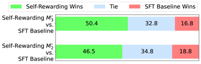<details> <summary>x8.png Details</summary>  ### Visual Description \n ## Stacked Bar Chart: Comparison of Self-Rewarding Models vs. SFT Baseline ### Overview The image presents a stacked bar chart comparing the performance of two self-rewarding models (M¹₂ and M²₂) against an SFT Baseline. The chart visualizes the proportion of wins, ties, and losses for each model in comparison to the baseline. Each bar represents a comparison, and is divided into three segments representing "Self-Rewarding Wins", "Tie", and "SFT Baseline Wins". ### Components/Axes * **Y-Axis:** Lists the two self-rewarding models being compared: "Self-Rewarding M¹₂ vs. SFT Baseline" and "Self-Rewarding M²₂ vs. SFT Baseline". * **X-Axis:** Represents the percentage of outcomes, with no explicit scale markings but values ranging from 0 to approximately 50. * **Legend:** Located at the top-left corner, defines the color coding: * Green: Self-Rewarding Wins * Light Blue: Tie * Red: SFT Baseline Wins ### Detailed Analysis The chart consists of two stacked bars, one for each model comparison. **1. Self-Rewarding M¹₂ vs. SFT Baseline:** * **Self-Rewarding Wins (Green):** Approximately 50.4%. * **Tie (Light Blue):** Approximately 32.8%. * **SFT Baseline Wins (Red):** Approximately 16.8%. **2. Self-Rewarding M²₂ vs. SFT Baseline:** * **Self-Rewarding Wins (Green):** Approximately 46.5%. * **Tie (Light Blue):** Approximately 34.8%. * **SFT Baseline Wins (Red):** Approximately 18.8%. ### Key Observations * Both self-rewarding models (M¹₂ and M²₂) demonstrate a higher proportion of wins compared to the SFT Baseline. * Model M¹₂ has a slightly higher win rate (50.4%) than Model M²₂ (46.5%). * The proportion of ties is relatively similar for both models, around 33-35%. * The SFT Baseline win rate is consistently lower for both comparisons, around 17-19%. ### Interpretation The data suggests that both self-rewarding models outperform the SFT Baseline in this comparison. The higher win rates for the self-rewarding models indicate that they are more effective at achieving favorable outcomes against the baseline. The difference in win rates between M¹₂ and M²₂ suggests that M¹₂ is slightly more effective than M²₂. The consistent presence of ties indicates that there are scenarios where neither model nor the baseline achieves a clear win. The data does not provide information on the nature of the tasks or the criteria for determining a "win", "tie", or "loss". Further investigation would be needed to understand the specific strengths and weaknesses of each model and the reasons for the observed performance differences. 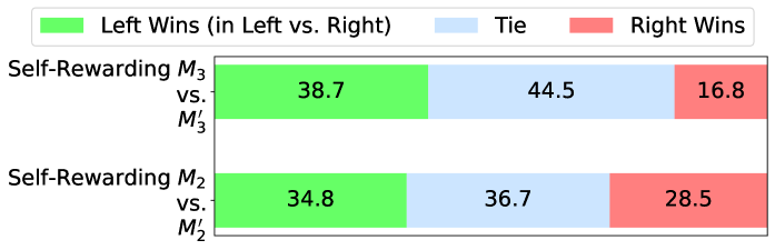</details> <details> <summary>x9.png Details</summary>  ### Visual Description \n ## Bar Chart: Comparison of Win Rates - Self-Rewarding Strategies ### Overview This is a horizontal bar chart comparing the win rates of two self-rewarding strategies (M3 vs. M'3 and M2 vs. M'2) in a left-vs-right competition. The chart displays the percentage of wins for the left strategy, ties, and wins for the right strategy for each comparison. ### Components/Axes * **Y-axis:** Represents the strategy comparison. Two comparisons are shown: "Self-Rewarding M3 vs. M'3" and "Self-Rewarding M2 vs. M'2". * **X-axis:** Represents the percentage of outcomes. The scale is not explicitly labeled, but ranges from approximately 0% to 50%. * **Legend (Top-Left):** * Green: Left Wins (in Left vs. Right) * Light Blue: Tie * Red: Right Wins ### Detailed Analysis The chart consists of two horizontal bars, each divided into three segments representing the win rates. **1. Self-Rewarding M3 vs. M'3:** * **Left Wins (Green):** The green segment occupies approximately the first half of the bar and is labeled "38.7". * **Tie (Light Blue):** The light blue segment follows the green segment and occupies roughly the middle portion of the bar. It is labeled "44.5". * **Right Wins (Red):** The red segment occupies the remaining portion of the bar and is labeled "16.8". **2. Self-Rewarding M2 vs. M'2:** * **Left Wins (Green):** The green segment occupies approximately the first third of the bar and is labeled "34.8". * **Tie (Light Blue):** The light blue segment follows the green segment and occupies roughly the middle portion of the bar. It is labeled "36.7". * **Right Wins (Red):** The red segment occupies the remaining portion of the bar and is labeled "28.5". ### Key Observations * In both comparisons, the "Tie" outcome has the highest percentage. * The M3 vs. M'3 comparison shows a relatively higher win rate for the left strategy (38.7%) compared to the M2 vs. M'2 comparison (34.8%). * The M2 vs. M'2 comparison has the highest win rate for the right strategy (28.5%) compared to the M3 vs. M'3 comparison (16.8%). ### Interpretation The data suggests that both self-rewarding strategies, M3 and M2, result in a significant number of ties when competing against their respective counterparts (M'3 and M'2). Strategy M3 appears to have a slight advantage in terms of left-side wins, while strategy M2 shows a higher proportion of right-side wins. The high tie rate across both comparisons indicates that the strategies are relatively balanced, or that the competition is often inconclusive. The differences in win rates between the left and right sides for each strategy could be due to inherent biases in the strategies themselves, or to the specific conditions of the competition. Further investigation would be needed to determine the underlying reasons for these observed patterns. </details> Figure 8: EFT data helps the self-rewarding loop: We evaluated the series of models trained using self-reward loops starting from the model trained using only IFT data. We performed head-to-head win rates comparisons on the IFT test set. While $M_{2}^{\prime}$ can improve over the SFT baseline and $M_{3}^{\prime}$ can improve even more over the SFT baseline, they lag far behind the corresponding models ( $M_{2}$ , $M_{3}$ ) that started from a base model trained using both IFT and EFT data, see Figure 3. <LIST ALL ALPACAEVAL INSTRUCTIONS> Given the above list of possible instructions, define a maximum of 20 categories that would cover the types of intructions, for example recipes, reasoning tasks, general knowledge etc. Try to cover as many of the instructions as possible with the maximum 20 categories, while keeping the categories high-level, simple and easy to understand. Figure 9: Prompt used to obtain instruction categories on the AlpacaEval test set. Instruction: <INSTRUCTION> Given the above, categorize it into one of the following 20 categories: <LIST ALL CATEGORIES> Secondly, score the instruction in terms of complexity: how complex you think it is to answer from 1-10 (where 10 is a complex question whereby first reasoning or breaking down the question into multiple subquestions for example might help improve the answer). Thirdly, indicate how long you think the response to the instruction should be, either (a) 1 sentence, (b) 1-3 sentences, (c) 1 paragraph, (d) 2 paragraphs, or (e) 3 or more paragraphs. Provide your final response in the following format: Category: < one of the 20 categories > Complexity: < score out of 10 > Length: < length category >. Do not provide the actual response. Figure 10: Prompt for categorizing instructions based on their topics, complexities and expected response lengths. Table 6: Breakdown of AlpacaEval test set instructions by instruction category. | Science / Technology / Engineering | 134 | 16.65% | | --- | --- | --- | | Professional / Business / Marketing | 77 | 9.57% | | Social Interaction / Relationships / Human Behavior | 68 | 8.45% | | Miscellaneous / Other | 61 | 7.58% | | Mathematics / Logical Reasoning | 52 | 6.46% | | Cooking / Recipes | 48 | 5.96% | | Software Development / Coding / Algorithms | 44 | 5.47% | | Travel / Geography / Exploration | 41 | 5.09% | | Literature / Writing / Communication | 39 | 4.84% | | History / Social Studies | 38 | 4.72% | | Entertainment / Media Analysis | 34 | 4.22% | | Language Learning / Linguistics | 32 | 3.98% | | Music / Audio / Arts | 30 | 3.73% | | DIY Projects / Hobbies | 24 | 2.98% | | Technology / Gadgets / Consumer Products | 20 | 2.48% | | Gaming / Game Development | 18 | 2.24% | | Exercise / Health / Wellness | 16 | 1.99% | | Philosophy / Ethics / Ideology | 15 | 1.86% | | Sports / Athletics / Physical Activity | 12 | 1.49% | | Strategy / Problem-Solving / Critical Thinking | 2 | 0.24% | Table 7: Breakdown of AlpacaEval test set instructions by instruction complexity. The instructions increase in complexity from 1 to 9, where 10 is a complex question that requires first reasoning or breaking the problem into sub-problems before it can be solved. | 3 | 238 | 29.57% | | --- | --- | --- | | 2 | 206 | 25.59% | | 4 | 122 | 15.16% | | 6 | 79 | 9.81% | | 5 | 68 | 8.45% | | 7 | 41 | 5.09% | | 1 | 34 | 4.22% | | 8 | 14 | 1.74% | | 9 | 3 | 0.37% | Table 8: Breakdown of AlpacaEval test set instructions by expected response length. 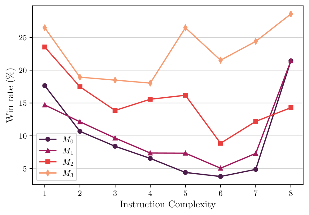| 1-3 sentences 1 paragraph 1 sentence | 361 269 143 | 44.84% 33.42% 17.76% | | --- | --- | --- | | 2 paragraphs | 31 | 3.85% | | 3 or more paragraphs | 1 | 0.13% | <details> <summary>x10.png Details</summary>  ### Visual Description \n ## Line Chart: Win Rate vs. Instruction Complexity ### Overview The image presents a line chart illustrating the relationship between Instruction Complexity (on the x-axis) and Win Rate (on the y-axis) for four different models (M₀, M₁, M₂, and M₃). The chart displays the win rate percentage as a function of increasing instruction complexity, ranging from 1 to 8. ### Components/Axes * **X-axis:** Instruction Complexity (ranging from 1 to 8). * **Y-axis:** Win rate (%), ranging from 0 to 30, with tick marks at 5, 10, 15, 20, 25, and 30. * **Legend:** Located in the top-left corner, identifying four data series: * M₀ (Dark Blue, circle marker) * M₁ (Gray, square marker) * M₂ (Red, triangle marker) * M₃ (Orange, diamond marker) * **Gridlines:** Horizontal gridlines are present to aid in reading the y-axis values. ### Detailed Analysis The chart displays four distinct lines, each representing a model's win rate across different instruction complexities. * **M₀ (Dark Blue):** The line slopes downward from x=1 to x=7, then sharply increases at x=8. * At x=1, Win Rate ≈ 17%. * At x=2, Win Rate ≈ 18%. * At x=3, Win Rate ≈ 10%. * At x=4, Win Rate ≈ 8%. * At x=5, Win Rate ≈ 5%. * At x=6, Win Rate ≈ 5%. * At x=7, Win Rate ≈ 5%. * At x=8, Win Rate ≈ 21%. * **M₁ (Gray):** The line generally decreases from x=1 to x=7, then increases slightly at x=8. * At x=1, Win Rate ≈ 15%. * At x=2, Win Rate ≈ 14%. * At x=3, Win Rate ≈ 13%. * At x=4, Win Rate ≈ 15%. * At x=5, Win Rate ≈ 16%. * At x=6, Win Rate ≈ 9%. * At x=7, Win Rate ≈ 10%. * At x=8, Win Rate ≈ 14%. * **M₂ (Red):** The line decreases from x=1 to x=4, then increases from x=4 to x=8. * At x=1, Win Rate ≈ 23%. * At x=2, Win Rate ≈ 17%. * At x=3, Win Rate ≈ 14%. * At x=4, Win Rate ≈ 15%. * At x=5, Win Rate ≈ 16%. * At x=6, Win Rate ≈ 8%. * At x=7, Win Rate ≈ 11%. * At x=8, Win Rate ≈ 15%. * **M₃ (Orange):** The line decreases from x=1 to x=6, then increases sharply from x=6 to x=8. * At x=1, Win Rate ≈ 26%. * At x=2, Win Rate ≈ 21%. * At x=3, Win Rate ≈ 18%. * At x=4, Win Rate ≈ 18%. * At x=5, Win Rate ≈ 24%. * At x=6, Win Rate ≈ 22%. * At x=7, Win Rate ≈ 27%. * At x=8, Win Rate ≈ 28%. ### Key Observations * M₀ exhibits the lowest win rates across most instruction complexities, with a significant jump at complexity 8. * M₃ consistently demonstrates the highest win rates, particularly at higher instruction complexities. * M₁ and M₂ show relatively similar performance, with M₂ experiencing a dip in win rate at complexity 6. * All models show a general trend of decreasing win rate as instruction complexity increases, except for a notable increase at complexity 8 for all models. ### Interpretation The data suggests that increasing instruction complexity generally reduces the win rate for all models, indicating a challenge in handling more complex tasks. However, the sharp increase in win rate at instruction complexity 8 for all models is a significant outlier. This could indicate a threshold effect, where the models perform better on tasks exceeding a certain complexity level, or it could be due to a specific characteristic of the tasks at complexity 8. M₃ consistently outperforms the other models, suggesting it is more robust to increasing instruction complexity. M₀, on the other hand, struggles with complexity, but shows a substantial improvement at the highest complexity level. This could be due to a different learning strategy or architecture. The relationship between instruction complexity and win rate is not strictly linear, as evidenced by the fluctuations in the lines. This suggests that the difficulty of a task is not solely determined by its complexity, but also by other factors. Further investigation is needed to understand the specific characteristics of the tasks at each complexity level and how they affect the performance of each model. 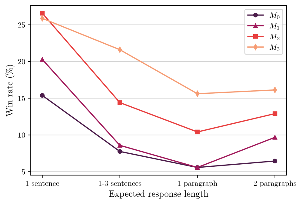</details> <details> <summary>x11.png Details</summary>  ### Visual Description \n ## Line Chart: Win Rate vs. Expected Response Length ### Overview This image presents a line chart illustrating the relationship between the expected response length and the win rate for four different models (M0, M1, M2, and M3). The x-axis represents the expected response length, categorized into four levels: "1 sentence", "1-3 sentences", "1 paragraph", and "2 paragraphs". The y-axis represents the win rate, measured in percentage (%). ### Components/Axes * **X-axis Title:** "Expected response length" * **Y-axis Title:** "Win rate (%)" * **X-axis Categories:** "1 sentence", "1-3 sentences", "1 paragraph", "2 paragraphs" * **Y-axis Scale:** Ranges from approximately 5% to 27%, with gridlines at 5%, 10%, 15%, 20%, and 25%. * **Legend:** Located in the top-right corner, identifying the four models: * M0 (Purple) * M1 (Dark Red) * M2 (Light Red) * M3 (Orange) ### Detailed Analysis Let's analyze each model's trend and extract data points: * **M0 (Purple):** The line slopes downward overall. * 1 sentence: Approximately 15% * 1-3 sentences: Approximately 8% * 1 paragraph: Approximately 6% * 2 paragraphs: Approximately 6% * **M1 (Dark Red):** The line initially decreases sharply, then increases slightly. * 1 sentence: Approximately 20% * 1-3 sentences: Approximately 8% * 1 paragraph: Approximately 10% * 2 paragraphs: Approximately 12% * **M2 (Light Red):** The line decreases steadily. * 1 sentence: Approximately 27% * 1-3 sentences: Approximately 23% * 1 paragraph: Approximately 10% * 2 paragraphs: Approximately 12% * **M3 (Orange):** The line decreases, but remains relatively stable. * 1 sentence: Approximately 25% * 1-3 sentences: Approximately 21% * 1 paragraph: Approximately 10% * 2 paragraphs: Approximately 17% ### Key Observations * Model M2 consistently exhibits the highest win rate at "1 sentence" and "1-3 sentences". * All models show a decrease in win rate as the expected response length increases from "1 sentence" to "1 paragraph". * M1, M2, and M3 show an increase in win rate from "1 paragraph" to "2 paragraphs", while M0 remains constant. * The win rates for M0, M1, M2, and M3 converge towards similar values at "1 paragraph" and "2 paragraphs". ### Interpretation The data suggests that shorter expected response lengths generally lead to higher win rates, particularly for Model M2. This could indicate that users prefer concise responses, or that the models are more accurate when generating shorter outputs. The increase in win rate for M1, M2, and M3 at "2 paragraphs" might suggest that these models can provide more valuable information when allowed a longer response format, while M0 does not benefit from the increased length. The convergence of win rates at longer response lengths could indicate a limit to the benefits of increased length, or that all models perform similarly when generating more detailed responses. The initial high win rate of M2 could be due to its specific training data or architecture, making it particularly well-suited for short-form responses. Further investigation would be needed to understand the underlying reasons for these trends and to optimize the models for different response length requirements. </details> Figure 11: AlpacaEval win rate breakdown for instruction complexities (left) and expected response lengths (right). Self-Rewarding models give gains across most complexities and all response length ranges. A.4 Preference optimization outperforms augmenting with positive examples only We also tried an alternative self-training procedure of adding high-quality self-instruction creation examples to supervised fine-tuning (without preference optimization), rather than DPO. In this variant, we add additional examples of (instruction prompt, response) curated by the model to the seed set for supervised fine-tuning, following other approaches [Li et al., 2024, Adolphs et al., 2023, Gulcehre et al., 2023], rather than constructing preference data. In this setup we only add examples where the candidate response was evaluated to give a perfect score of $r_{i}^{n}=5$ . Unfortunately we could not find a configuration where this approach helped. For example, adding 11,254 such examples that scored 5 out of 5, and optimizing the mixing weight in training, still yielded a head to head with the SFT Baseline of 29% wins vs 30% wins, i.e., no improvement. A.5 Augmented Prompt Generation Using Newly Trained Models In our experiments, for time efficiency, we have created a fixed pool of augmented prompts in advance using ChatLlama 70B. In a real interactive system, ideally, those prompts could come from real users so that we can ensure the models are trained to align with real user requirements. Here, we also examine whether our newly trained Self-Rewarding models in each iteration can generate new prompts through in-context learning, instead of using ChatLlama 70B. To check this, we constructed 30 prompts with in-context examples using the original seed IFT data as described in Section 2.2 and tested whether $M_{1}$ , $M_{2}$ and $M_{3}$ still possess in-context learning ability and can generate high quality instructions. According to manual inspection, all models can generate novel instructions given in-context examples in all 30 cases. However, for $M2$ and $M3$ , the model is likely to first generate a few instructions, then generate a separator, and then start responding to the instructions, so some postprocessing might be necessary. A.6 AlpacaEval Test Sample Clustering We used the GPT-4 (gpt-4-1106-preview) model to categorize the instructions in the AlpacaEval test set into clusters from three perspectives: (1) instruction category, (2) instruction complexity, and (3) expected response length. To obtain instruction categories for the AlpaceEval test set, we used the prompt in Figure 9 and obtained 20 categories in total. Then, to cluster the instructions into different groups, we use the prompt in Figure 10 for each test example. The corresponding statistics are given in Table 6, Table 7, Table 8. The fine-grained results on instruction complexity and expected response length are given in Figure 11. Table 9: NLP Benchmarks. Self-Rewarding models mostly tend to maintain performance compared to the Llama 2 base model and the SFT Baseline, despite being fine-tuned on very different instruction-following prompts. | Llama 2 SFT Baseline $M_{1}$ | 80.20 76.49 78.14 | 57.40 55.97 57.51 | 85.30 85.17 84.99 | 50.70 51.48 53.02 | 82.80 82.59 82.92 | 56.80 50.72 60.27 | 68.90 69.76 69.34 | 60.20 57.80 57.60 | 25.30 34.35 35.48 | | --- | --- | --- | --- | --- | --- | --- | --- | --- | --- | | $M_{2}$ | 74.84 | 54.51 | 84.27 | 51.23 | 81.94 | 59.29 | 69.31 | 57.60 | 33.07 | | $M_{3}$ | 72.35 | 53.13 | 83.29 | 49.28 | 80.79 | 57.70 | 69.37 | 58.40 | 31.86 | Table 10: MT-Bench Fine-grained Results. We list our models’ performance on each problem category. Self-reward is especially effective in improving the model’s ability in writing, role-playing, extraction, and STEM tasks. | SFT M1 M2 | 8.83 9.10 9.10 | 8.15 7.65 8.00 | 5.30 4.35 4.60 | 3.00 3.05 3.30 | 3.50 4.10 4.25 | 6.90 7.20 7.65 | 9.18 8.93 9.40 | 9.95 9.85 9.80 | 6.85 6.78 7.01 | | --- | --- | --- | --- | --- | --- | --- | --- | --- | --- | | M3 | 9.58 | 8.73 | 4.80 | 3.50 | 4.20 | 7.80 | 9.45 | 9.95 | 7.25 | A.7 NLP Benchmark Results and MT-Bench Results We provide the detailed model performance on a number of NLP benchmarks in Table 9 and on MT-Bench in Table 10. In particular, some NLP benchmarks including ARC-Challenge, HellaSwag, SIQA, PIQA, and OBQA are all text completion tasks. In these tasks, given the multiple choice options, we choose the option corresponding to the highest log probability scored by the models as the final answer. As such, the objective of these particular tasks is quite different from what our algorithm tries to optimize, so the results on these tasks may not reflect the true capability of our models.