# Medusa: Simple LLM Inference Acceleration Framework with Multiple Decoding Heads
**Authors**: Tianle Cai, Yuhong Li, Zhengyang Geng, Hongwu Peng, Jason D. Lee, Deming Chen, Tri Dao
Abstract
Large Language Models (LLMs) employ auto-regressive decoding that requires sequential computation, with each step reliant on the previous one’s output. This creates a bottleneck as each step necessitates moving the full model parameters from High-Bandwidth Memory (HBM) to the accelerator’s cache. While methods such as speculative decoding have been suggested to address this issue, their implementation is impeded by the challenges associated with acquiring and maintaining a separate draft model. In this paper, we present Medusa, an efficient method that augments LLM inference by adding extra decoding heads to predict multiple subsequent tokens in parallel. Using a tree-based attention mechanism, Medusa constructs multiple candidate continuations and verifies them simultaneously in each decoding step. By leveraging parallel processing, Medusa substantially reduces the number of decoding steps required. We present two levels of fine-tuning procedures for Medusa to meet the needs of different use cases: Medusa -1: Medusa is directly fine-tuned on top of a frozen backbone LLM, enabling lossless inference acceleration. Medusa -2: Medusa is fine-tuned together with the backbone LLM, enabling better prediction accuracy of Medusa heads and higher speedup but needing a special training recipe that preserves the model’s capabilities. Moreover, we propose several extensions that improve or expand the utility of Medusa, including a self-distillation to handle situations where no training data is available and a typical acceptance scheme to boost the acceptance rate while maintaining generation quality. We evaluate Medusa on models of various sizes and training procedures. Our experiments demonstrate that Medusa -1 can achieve over 2.2 $×$ speedup without compromising generation quality, while Medusa -2 further improves the speedup to 2.3-2.8 $×$ .
Machine Learning, ICML
1 Introduction
The recent advancements in Large Language Models (LLMs) have demonstrated that the quality of language generation significantly improves with an increase in model size, reaching billions of parameters (Brown et al., 2020; Chowdhery et al., 2022; Zhang et al., 2022; Hoffmann et al., 2022; OpenAI, 2023; Google, 2023; Touvron et al., 2023). However, this growth has led to an increase in inference latency, which poses a significant challenge in practical applications. From a system perspective, LLM inference is predominantly memory-bandwidth-bound (Shazeer, 2019; Kim et al., 2023), with the main latency bottleneck stemming from accelerators’ memory bandwidth rather than arithmetic computations. This bottleneck is inherent to the sequential nature of auto-regressive decoding, where each forward pass requires transferring the complete model parameters from High-Bandwidth Memory (HBM) to the accelerator’s cache. This process, which generates only a single token, underutilizes the arithmetic computation potential of modern accelerators, leading to inefficiency.
To address this, one approach to speed up LLM inference involves increasing the arithmetic intensity (the ratio of total floating-point operations (FLOPs) to total data movement) of the decoding process and reducing the number of decoding steps. In line with this idea, speculative decoding has been proposed (Leviathan et al., 2022; Chen et al., 2023; Xia et al., 2023; Miao et al., 2023). This method uses a smaller draft model to generate a token sequence, which is then refined by the original, larger model for acceptable continuation. However, obtaining an appropriate draft model remains challenging, and it’s even harder to integrate the draft model into a distributed system (Chen et al., 2023).
Instead of using a separate draft model to sequentially generate candidate outputs, in this paper, we revisit and refine the concept of using multiple decoding heads on top of the backbone model to expedite inference (Stern et al., 2018). We find that when applied effectively, this technique can overcome the challenges of speculative decoding, allowing for seamless integration into existing LLM systems. Specifically, we introduce Medusa, a method that enhances LLM inference by integrating additional decoding heads to concurrently predict multiple tokens. These heads are fine-tuned in a parameter-efficient manner and can be added to any existing model. With no requirement for a draft model, Medusa offers easy integration into current LLM systems, including those in distributed environments, ensuring a user-friendly experience.
We further enhance Medusa with two key insights. Firstly, the current approach of generating a single candidate continuation at each decoding step leads to inefficient use of computational resources. To address this, we propose generating multiple candidate continuations using the Medusa heads and verifying them concurrently through a simple adjustment to the attention mask. Secondly, we can reuse the rejection sampling scheme as used in speculative decoding (Leviathan et al., 2022; Chen et al., 2023) to generate consistent responses with the same distribution as the original model. However, it cannot further enhance the acceleration rate. Alternatively, we introduce a typical acceptance scheme that selects reasonable candidates from the Medusa head outputs. We use temperature as a threshold to manage deviation from the original model’s predictions, providing an efficient alternative to the rejection sampling method. Our results suggest that the proposed typical acceptance scheme can accelerate the decoding speed further while maintaining a similar generation quality.
To equip LLMs with predictive Medusa heads, we propose two distinct fine-tuning procedures tailored to various scenarios. For situations with limited computational resources or when the objective is to incorporate Medusa into an existing model without affecting its performance, we recommend Medusa -1. This method requires minimal memory and can be further optimized with quantization techniques akin to those in QLoRA (Dettmers et al., 2023), without compromising the generation quality due to the fixed backbone model. However, in Medusa -1, the full potential of the backbone model is not utilized. We can further fine-tune it to enhance the prediction accuracy of Medusa heads, which can directly lead to a greater speedup. Therefore, we introduce Medusa -2, which is suitable for scenarios with ample computational resources or for direct Supervised Fine-Tuning (SFT) from a base model. The key to Medusa -2 is a training protocol that enables joint training of the Medusa heads and the backbone model without compromising the model’s next-token prediction capability and output quality. We propose different strategies for obtaining the training datasets depending on the model’s training recipe and dataset availability. When the model is fine-tuned on a public dataset, it can be directly used for Medusa. If the dataset is unavailable or the model underwent a Reinforcement Learning with Human Feedback (RLHF) (Ouyang et al., 2022) process, we suggest a self-distillation approach to generate a training dataset for the Medusa heads.
Our experiments primarily focus on scenarios with a batch size of one, which is representative of the use case where LLMs are locally hosted for personal use. We test Medusa on models of varying sizes and training settings, including Vicuna-7B, 13B (trained with a public dataset), Vicuna-33B (Chiang et al., 2023) (trained with a private dataset Upon contacting the authors, this version is experimental and used some different data than Vicuna 7B and 13B.), and Zephyr-7B (trained with both supervised fine-tuning and alignment). Medusa can achieve a speedup of 2.3 to 2.8 times across different prompt types without compromising on the quality of generation.
<details>
<summary>x1.png Details</summary>
### Visual Description
# Technical Diagram Analysis: Medusa Architecture for LLM Acceleration
This document provides a detailed technical extraction of the provided architectural diagram, which illustrates the "Medusa" method for accelerating Large Language Model (LLM) inference.
## 1. Component Isolation
The diagram is organized into five primary functional regions:
1. **Header:** Branding/Logo.
2. **Original Model (Blue Block):** The base transformer architecture.
3. **Medusa Heads (Red Block):** The parallel prediction heads.
4. **Top-k Predictions (Purple Block):** The output tokens from each head.
5. **Footer/Processing Logic:** Input, candidate verification, and final prediction.
---
## 2. Detailed Component Extraction
### Header
* **Logo:** A circular emblem featuring a stylized llama with a star above its head, framed by wavy hair reminiscent of the Starbucks logo (a play on "Medusa" and "Llama").
### Original Model (Blue Region - Left)
This region represents the standard frozen or base model.
* **Labels:** ❄️ / 🔥 Original Model
* **Internal Flow:**
* **Embedding:** The entry point for input data.
* **Transformer Layers:** The core processing block.
* **LM Head:** The standard Language Modeling head that predicts the next token.
* **Data Path:** An arrow labeled **"Last Hidden"** originates from the output of the Transformer Layers and branches to both the LM Head and the Medusa Heads.
### Medusa Heads (Red Region - Center)
This region represents the additional heads added to the model.
* **Label:** 🔥 Medusa Heads
* **Components:**
* **Medusa Head 1**
* **Medusa Head 2**
* **Medusa Head 3**
* **Input:** All three heads receive the "Last Hidden" state from the Transformer Layers in parallel.
### Top-k Predictions (Purple Region - Right)
This region displays the candidate tokens generated by each head.
* **Label:** 🔝 Top-$k$ Predictions
* **Data Mapping:**
| Source | Predictions |
| :--- | :--- |
| **LM Head** | "It, I, As" |
| **Medusa Head 1** | "is, ', the" |
| **Medusa Head 2** | "difficult, is, '" |
| **Medusa Head 3** | "not, difficult, a" |
### Footer / Logic Flow (Bottom)
* **Input Block:**
* **Label:** 📝 Input
* **Text:** "What will happen if Medusa meets a Llama?"
* **Candidates Block:**
* **Label:** 📜 Candidates
* **Content:**
* **It is difficult** not ✅ (Indicated as the correct/accepted sequence)
* **It'** difficult a ❌
* **It is'** not ❌
* ... (Ellipsis indicating further candidates)
* **Single Step Prediction Block:**
* **Label:** ✍️ Single step prediction
* **Text:** *It is difficult*
---
## 3. Process Flow and Logic
1. **Input Processing:** The text "What will happen if Medusa meets a Llama?" is fed into the **Embedding** layer and processed through **Transformer Layers**.
2. **Parallel Generation:** Instead of generating one token, the **Last Hidden** state is sent to the **LM Head** and three **Medusa Heads** simultaneously.
3. **Token Proposal:**
* The LM Head predicts the immediate next token (e.g., "It").
* Medusa Head 1 predicts the token after that (e.g., "is").
* Medusa Head 2 predicts the third token (e.g., "difficult").
* Medusa Head 3 predicts the fourth token (e.g., "not").
4. **Candidate Assembly:** The system combines the top-$k$ results from all heads to create multiple potential sentence continuations (Candidates).
5. **Verification:** The candidates are checked for linguistic validity.
* The sequence "**It is difficult**" is validated.
* Incorrect combinations like "**It' difficult**" are rejected.
6. **Output:** In a **Single step prediction**, the model successfully outputs multiple tokens (*It is difficult*) at once, rather than generating them one by one, thereby increasing inference speed.
## 4. Symbol Legend
* ❄️: Likely represents "Frozen" parameters (Original Model).
* 🔥: Likely represents "Trainable" parameters (Medusa Heads).
* ✅: Validated/Accepted candidate.
* ❌: Rejected candidate.
</details>
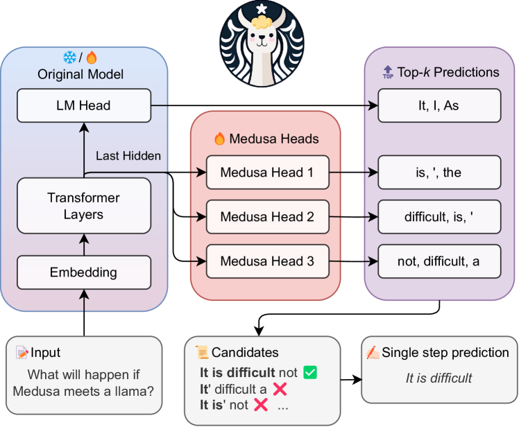
Figure 1: Medusa introduces multiple heads on top of the last hidden states of the LLM, enabling the prediction of several subsequent tokens in parallel (Section 2.1.1). During inference, each head generates multiple top predictions for its designated position. These predictions are assembled into candidates, which are processed in parallel using a tree-based attention mechanism (Section 2.1.2). The final step is to verify the candidates and accept a continuation. Besides the standard rejection sampling scheme, a typical acceptance scheme (Section 2.3.1) can also be used here to select reasonable continuations, and the longest accepted candidate prefix will be used for the next decoding phase.
2 Methodology
Medusa follows the same framework as speculative decoding, where each decoding step primarily consists of three substeps: (1) generating candidates, (2) processing candidates, and (3) accepting candidates. For Medusa, (1) is achieved by Medusa heads, (2) is realized by tree attention, and since Medusa heads are on top of the original model, the logits calculated in (2) can be used for substep (1) for the next decoding step. The final step (3) can be realized by either rejection sampling (Leviathan et al., 2022; Chen et al., 2023) or typical acceptance (Section 2.3.1). The overall pipeline is illustrated in Figure 1.
In this section, we first introduce the key components of Medusa, including Medusa heads, and tree attention. Then, we present two levels of fine-tuning procedures for Medusa to meet the needs of different use cases. Finally, we propose two extensions to Medusa, including self-distillation and typical acceptance, to handle situations where no training data is available for Medusa and to improve the efficiency of the decoding process, respectively.
2.1 Key Components
2.1.1 Medusa Heads
In speculative decoding, subsequent tokens are predicted by an auxiliary draft model. This draft model must be small yet effective enough to generate continuations that the original model will accept. Fulfilling these requirements is a challenging task, and existing approaches (Spector & Re, 2023; Miao et al., 2023) often resort to separately pre-training a smaller model. This pre-training process demands substantial additional computational resources. For example, in (Miao et al., 2023), a reported 275 NVIDIA A100 GPU hours were used. Additionally, separate pre-training can potentially create a distribution shift between the draft model and the original model, leading to continuations that the original model may not favor. Chen et al. (2023) have also highlighted the complexities of serving multiple models in a distributed environment.
To streamline and democratize the acceleration of LLM inference, we take inspiration from Stern et al. (2018), which utilizes parallel decoding for tasks such as machine translation and image super-resolution. Medusa heads are additional decoding heads appended to the last hidden states of the original model. Specifically, given the original model’s last hidden states $h_{t}$ at position $t$ , we add $K$ decoding heads to $h_{t}$ . The $k$ -th head is used to predict the token in the $(t+k+1)$ -th position of the next tokens (the original language model head is used to predict the $(t+1)$ -th position). The prediction of the $k$ -th head is denoted as $p_{t}^{(k)}$ , representing a distribution over the vocabulary, while the prediction of the original model is denoted as $p_{t}^{(0)}$ . Following the approach of Stern et al. (2018), we utilize a single layer of feed-forward network with a residual connection for each head. We find that this simple design is sufficient to achieve satisfactory performance. The definition of the $k$ -th head is outlined as:
| | $\displaystyle p_{t}^{(k)}=\text{softmax}\left(W_{2}^{(k)}·\left(\text{SiLU%
}(W_{1}^{(k)}· h_{t})+h_{t}\right)\right),$ | |
| --- | --- | --- |
$d$ is the output dimension of the LLM’s last hidden layer and $V$ is the vocabulary size. We initialize $W_{2}^{(k)}$ identically to the original language model head, and $W_{1}^{(k)}$ to zero. This aligns the initial prediction of Medusa heads with that of the original model. The SiLU activation function (Elfwing et al., 2017) is employed following the Llama models (Touvron et al., 2023).
Unlike a draft model, Medusa heads are trained in conjunction with the original backbone model, which can remain frozen during training (Medusa -1) or be trained together (Medusa -2). This method allows for fine-tuning large models even on a single GPU, taking advantage of the powerful base model’s learned representations. Furthermore, it ensures that the distribution of the Medusa heads aligns with that of the original model, thereby mitigating the distribution shift problem. Additionally, since the new heads consist of just a single layer akin to the original language model head, Medusa does not add complexity to the serving system design and is friendly to distributed settings. We will discuss the training recipe for Medusa heads in Section 2.2.
2.1.2 Tree Attention
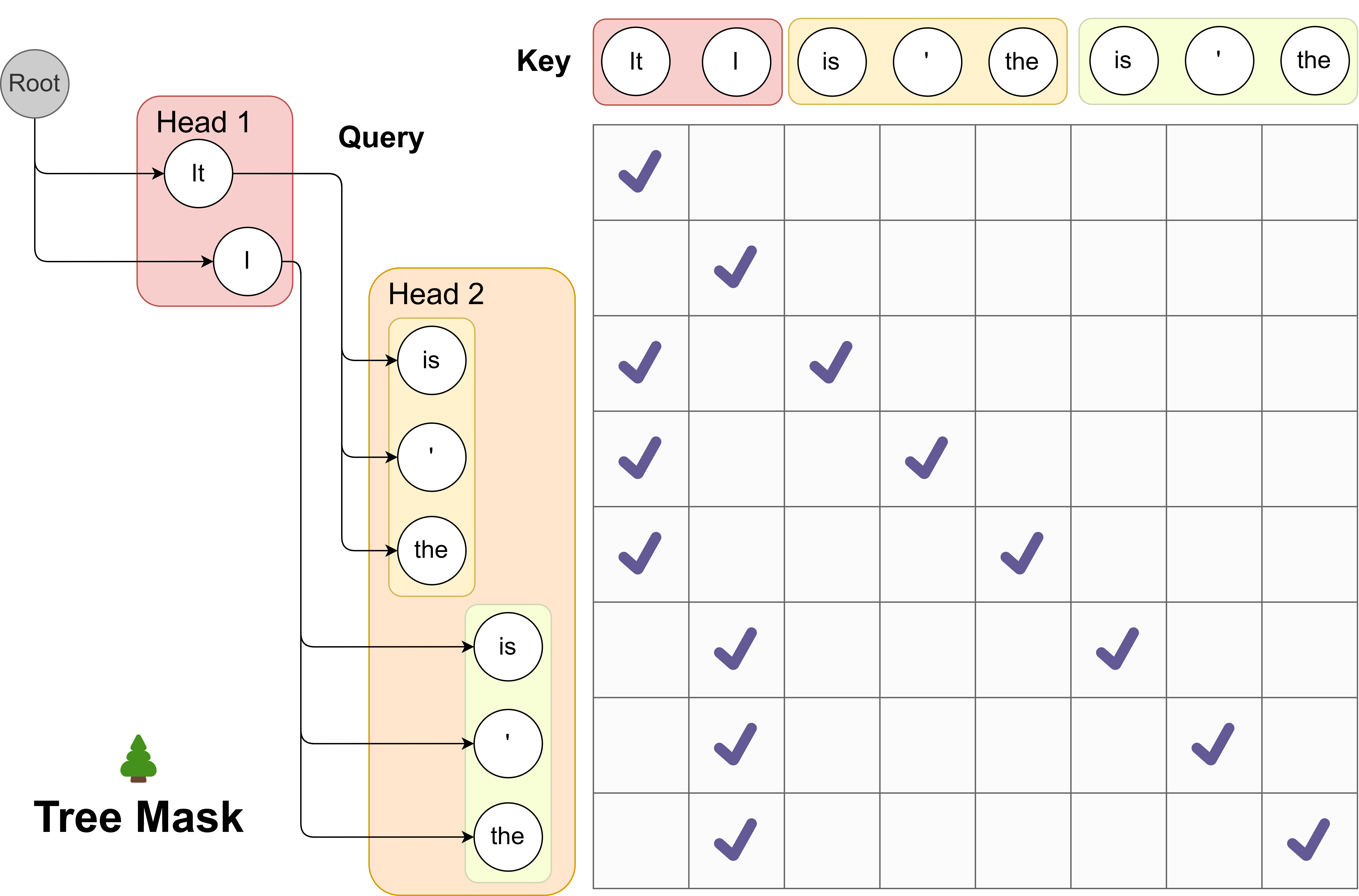
Through Medusa heads, we obtain probability predictions for the subsequent $K+1$ tokens. These predictions enable us to create length- $K+1$ continuations as candidates. While the speculative decoding studies (Leviathan et al., 2022; Chen et al., 2023) suggest sampling a single continuation as the candidate, leveraging multiple candidates during decoding can enhance the expected acceptance length within a decoding step. Nevertheless, more candidates can also raise computational demands. To strike a balance, we employ a tree-structured attention mechanism to process multiple candidates concurrently.
<details>
<summary>extracted/5668658/tree_attention.png Details</summary>
### Visual Description
# Technical Document Extraction: Tree Mask Attention Mechanism
This document describes a technical diagram illustrating a "Tree Mask" mechanism, likely used in Transformer-based architectures for processing hierarchical or branching data structures.
## 1. Component Isolation
The image is divided into three primary functional regions:
* **Left (Tree Structure):** A hierarchical representation of tokens starting from a "Root" node.
* **Top (Key Sequence):** A horizontal sequence of tokens acting as the "Key" in an attention mechanism.
* **Center-Right (Attention Matrix):** An $8 \times 8$ grid representing the mask, where checkmarks indicate permitted attention connections between "Query" tokens (rows) and "Key" tokens (columns).
---
## 2. Tree Structure and Query Mapping (Left Region)
The diagram shows how tokens are branched from a central root, organized into "Heads" (likely representing different branches or paths).
### Hierarchy Flow:
1. **Root (Grey Node):** The origin point.
2. **Head 1 (Red Background):** Contains two tokens:
* **It**
* **I**
3. **Head 2 (Orange Background):** This head branches further into two sub-groups based on the parent token from Head 1.
* **Sub-group 1 (Yellow Background):** Derived from the token "It". Contains: **is**, **'**, **the**.
* **Sub-group 2 (Green Background):** Derived from the token "I". Contains: **is**, **'**, **the**.
### Query Sequence (Vertical Axis):
The tokens from the tree are flattened into a vertical sequence of 8 rows for the attention matrix:
1. **It** (from Head 1)
2. **I** (from Head 1)
3. **is** (from Head 2, yellow)
4. **'** (from Head 2, yellow)
5. **the** (from Head 2, yellow)
6. **is** (from Head 2, green)
7. **'** (from Head 2, green)
8. **the** (from Head 2, green)
---
## 3. Key Sequence (Top Region)
The horizontal axis represents the **Key** tokens. They are grouped by color to match the tree structure:
* **Red Group:** [It], [I]
* **Yellow Group:** [is], ['], [the]
* **Green Group:** [is], ['], [the]
---
## 4. Attention Matrix (Tree Mask Data)
The matrix defines which Query (row) can attend to which Key (column). A purple checkmark ($\checkmark$) indicates an active connection.
### Data Table Reconstruction
| Query \ Key | It (Red) | I (Red) | is (Yel) | ' (Yel) | the (Yel) | is (Grn) | ' (Grn) | the (Grn) |
| :--- | :---: | :---: | :---: | :---: | :---: | :---: | :---: | :---: |
| **It** | $\checkmark$ | | | | | | | |
| **I** | | $\checkmark$ | | | | | | |
| **is (Yel)** | $\checkmark$ | | $\checkmark$ | | | | | |
| **' (Yel)** | $\checkmark$ | | | $\checkmark$ | | | | |
| **the (Yel)** | $\checkmark$ | | | | $\checkmark$ | | | |
| **is (Grn)** | | $\checkmark$ | | | | $\checkmark$ | | |
| **' (Grn)** | | $\checkmark$ | | | | | $\checkmark$ | |
| **the (Grn)** | | $\checkmark$ | | | | | | $\checkmark$ |
---
## 5. Trend and Logic Verification
* **Identity Attention:** Every token attends to itself, forming a sparse diagonal pattern (visible in the checkmarks at [1,1], [2,2], [3,3], etc.).
* **Hierarchical Dependency:**
* The **Yellow Group** (is, ', the) only attends to itself and its parent token **"It"** (Red). It cannot see the "I" (Red) branch or the Green branch.
* The **Green Group** (is, ', the) only attends to itself and its parent token **"I"** (Red). It cannot see the "It" (Red) branch or the Yellow branch.
* **Isolation:** There is no cross-attention between the Yellow and Green branches, despite them containing the same string literals ("is", "'", "the"). This confirms the mask enforces the tree structure where branches are independent.
## 6. Textual Labels Summary
* **Title:** Tree Mask (accompanied by a small evergreen tree icon 🌲).
* **Labels:** Root, Head 1, Head 2, Query, Key.
* **Tokens:** It, I, is, ', the.
</details>
Figure 2: We demonstrates the use of tree attention to process multiple candidates concurrently. As exemplified, the top-2 predictions from the first Medusa head and the top-3 from the second result in a total of $2× 3=6$ candidates. Each of these candidates corresponds to a distinct branch within the tree structure. To guarantee that each token only accesses its predecessors, we devise an attention mask that exclusively permits attention flow from the current token back to its antecedent tokens. The positional indices for positional encoding are adjusted in line with this structure.
This attention mechanism diverges from the traditional causal attention paradigm. Within this framework, only tokens from the same continuation are regarded as historical data. Drawing inspiration from the concept of embedding graph structures into attention as proposed in the graph neural network domain (Ying et al., 2021), we incorporate the tree structure into our attention mask, visualized in Figure 2. Remarkably, similar ideas have also been explored in independent works like Miao et al. (2023); Spector & Re (2023), where they follow a bottom-up approach and construct the tree by merging multiple candidates generated by a draft model. In our method, we instead take a top-down approach to build the tree thanks to the structure of candidates generated by Medusa heads. For a given $k$ -th head, its top- $s_{k}$ predictions serve as the basis for candidate formation, where $s_{k}$ is a designated hyperparameter. These candidates are established by determining the Cartesian product of the top- $s_{k}$ predictions from each head. For instance, in Figure 2, with $s_{1}=2$ and $s_{2}=3$ , each first head prediction can be succeeded by any prediction from the second head. This leads to a tree structure where $s_{k}$ branches exist at the $k$ -th level (considering a virtual root as the $0 0$ -level, in practice, this $0 0$ -level is for the prediction of the language model head of the original model, which can be sampled independently). Within this tree, only a token’s predecessors are seen as historical context, and our attention mask ensures that the attention is only applied on a token’s predecessors. By employing this mask and properly setting the positional indices for positional encoding, we can process numerous candidates simultaneously without the need to expand the batch size. The cumulative number of new tokens is calculated as $\sum_{k=1}^{K}\prod_{i=1}^{k}s_{i}$ .
In this section, we demonstrate the most simple and regular way to construct the tree structure by taking the Cartesian product. However, it is possible to construct the tree structure in a more sophisticated way and exploit the unbalanced accuracy of different top predictions of different heads. We will discuss this in Section 2.3.3.
2.2 Training Strategies
At the most basic level, we can train Medusa heads by freezing the backbone model and fine-tuning Medusa heads. However, training the backbone in conjunction with the Medusa heads can significantly enhance the accuracy of the Medusa heads. Depending on the computational resources and the specific reqirements of the use case, we propose two levels of training strategies for Medusa heads.
In this section, we assume the availability of a training dataset that aligns with the target model’s output distribution. This could be the dataset used for Supervised Fine-Tuning (SFT) of the target model. We will discuss eliminating the need for such a dataset using a self-distillation approach in Section 2.3.2.
2.2.1 Medusa -1: Frozen Backbone
To train Medusa heads with a frozen backbone model, we can use the cross-entropy loss between the prediction of Medusa heads and the ground truth. Specifically, given the ground truth token $y_{t+k+1}$ at position $t+k+1$ , the loss for the $k$ -th head is $\mathcal{L}_{k}=-\log p_{t}^{(k)}(y_{t+k+1})$ where $p_{t}^{(k)}(y)$ denotes the probability of token $y$ predicted by the $k$ -th head. We also observe that $\mathcal{L}_{k}$ is larger when $k$ is larger, which is reasonable since the prediction of the $k$ -th head is more uncertain when $k$ is larger. Therefore, we can add a weight $\lambda_{k}$ to $\mathcal{L}_{k}$ to balance the loss of different heads. And the total Medusa loss is:
$$
\displaystyle\mathcal{L}_{\text{{Medusa}-1}}=\sum_{k=1}^{K}-\lambda_{k}\log p_%
{t}^{(k)}(y_{t+k+1}). \tag{1}
$$
In practice, we set $\lambda_{k}$ as the $k$ -th power of a constant like $0.8$ . Since we only use the backbone model for providing the hidden states, we can use a quantized version of the backbone model to reduce the memory consumption. This introduces a more democratized way to accelerate LLM inference, as with the quantization, Medusa can be trained for a large model on a single consumer GPU similar to QLoRA (Dettmers et al., 2023). The training only takes a few hours (e.g., 5 hours for Medusa -1 on Vicuna 7B model with a single NVIDIA A100 PCIE GPU to train on 60k ShareGPT samples).
2.2.2 Medusa -2: Joint Training
To further improve the accuracy of Medusa heads, we can train Medusa heads together with the backbone model. However, this requires a special training recipe to preserve the backbone model’s next-token prediction capability and output quality. To achieve this, we propose three strategies:
- Combined loss: To keep the backbone model’s next-token prediction capability, we need to add the cross-entropy loss of the backbone model $\mathcal{L}_{\text{LM}}=-\log p_{t}^{(0)}(y_{t+1})$ to the Medusa loss. We also add a weight $\lambda_{0}$ to balance the loss of the backbone model and the Medusa heads. Therefore, the total loss is:
$$
\displaystyle\mathcal{L}_{\text{{Medusa}-2}}=\mathcal{L}_{\text{LM}}+\lambda_{%
0}\mathcal{L}_{\text{{Medusa}-1}}. \tag{2}
$$
- Differential learning rates: Since the backbone model is already well-trained and the Medusa heads need more training, we can use separate learning rates for them to enable faster convergence of Medusa heads while preserving the backbone model’s capability.
- Heads warmup: Noticing that at the beginning of training, the Medusa heads have a large loss, which leads to a large gradient and may distort the backbone model’s parameters. Following the idea from Kumar et al. (2022), we can employ a two-stage training process. In the first stage, we only train the Medusa heads as Medusa -1. In the second stage, we train the backbone model and Medusa heads together with a warmup strategy. Specifically, we first train the backbone model for a few epochs, then train the Medusa heads together with the backbone model. Besides this simple strategy, we can also use a more sophisticated warmup strategy by gradually increasing the weight $\lambda_{0}$ of the backbone model’s loss. We find both strategies work well in practice.
Putting these strategies together, we can train Medusa heads together with the backbone model without hurting the backbone model’s capability. Moreover, this recipe can be applied together with Supervised Fine-Tuning (SFT), enabling us to get a model with native Medusa support.
2.2.3 How to Select the Number of Heads
Empirically, we found that five heads are sufficient at most. Therefore, we recommend training with five heads and referring to the strategy described in Section 2.3.3 to determine the optimal configuration of the tree attention. With optimized tree attention, sometimes three or four heads may be enough for inference. In this case, we can ignore the redundant heads without overhead.
2.3 Extensions
2.3.1 Typical Acceptance
In speculative decoding papers (Leviathan et al., 2022; Chen et al., 2023), authors employ rejection sampling to yield diverse outputs that align with the distribution of the original model. However, subsequent implementations (Joao Gante, 2023; Spector & Re, 2023) reveal that this sampling strategy results in diminished efficiency as the sampling temperature increases. Intuitively, this can be comprehended in the extreme instance where the draft model is the same as the original one: Using greedy decoding, all output of the draft model will be accepted, therefore maximizing the efficiency. Conversely, rejection sampling introduces extra overhead, as the draft model and the original model are sampled independently. Even if their distributions align perfectly, the output of the draft model may still be rejected.
However, in real-world scenarios, sampling from language models is often employed to generate diverse responses, and the temperature parameter is used merely to modulate the “creativity” of the response. Therefore, higher temperatures should result in more opportunities for the original model to accept the draft model’s output. We ascertain that it is typically unnecessary to match the distribution of the original model. Thus, we propose employing a typical acceptance scheme to select plausible candidates rather than using rejection sampling. This approach draws inspiration from truncation sampling studies (Hewitt et al., 2022) (refer to Appendix A for an in-depth explanation). Our objective is to choose candidates that are typical, meaning they are not exceedingly improbable to be produced by the original model. We use the prediction probability from the original model as a natural gauge for this and establish a threshold based on the prediction distribution to determine acceptance. Specifically, given $x_{1},x_{2},·s,x_{n}$ as context, when evaluating the candidate sequence $(x_{n+1},x_{n+2},·s,x_{n+K+1})$ (composed by top predictions of the original language model head and Medusa heads), we consider the condition
| | $\displaystyle p_{\text{original}}(x_{n+k}|x_{1},x_{2},·s,x_{n+k-1})>$ | |
| --- | --- | --- |
where $H(·)$ denotes the entropy function, and $\epsilon,\delta$ are the hard threshold and the entropy-dependent threshold respectively. This criterion is adapted from Hewitt et al. (2022) and rests on two observations: (1) tokens with relatively high probability are meaningful, and (2) when the distribution’s entropy is high, various continuations may be deemed reasonable. During decoding, every candidate is evaluated using this criterion, and a prefix of the candidate is accepted if it satisfies the condition. To guarantee the generation of at least one token at each step, we apply greedy decoding for the first token and unconditionally accept it while employing typical acceptance for subsequent tokens. The final prediction for the current step is determined by the longest accepted prefix among all candidates.
Examining this scheme leads to several insights. Firstly, when the temperature is set to $0 0$ , it reverts to greedy decoding, as only the most probable token possesses non-zero probability. As the temperature surpasses $0 0$ , the outcome of greedy decoding will consistently be accepted with appropriate $\epsilon,\delta$ , since those tokens have the maximum probability, yielding maximal speedup. Likewise, in general scenarios, an increased temperature will correspondingly result in longer accepted sequences, as corroborated by our experimental findings.
Empirically, we verify that typical acceptance can achieve a better speedup while maintaining a similar generation quality as shown in Figure 5.
2.3.2 Self-Distillation
In Section 2.2, we assume the existence of a training dataset that matches the target model’s output distribution. However, this is not always the case. For example, the model owners may only release the model without the training data, or the model may have gone through a Reinforcement Learning with Human Feedback (RLHF) procedure, which makes the output distribution of the model different from the training dataset. To tackle this issue, we propose an automated self-distillation pipeline to use the model itself to generate the training dataset for Medusa heads, which matches the output distribution of the model.
The dataset generation process is straightforward. We first take a public seed dataset from a domain similar to the target model; for example, using the ShareGPT (ShareGPT, 2023) dataset for chat models. Then, we simply take the prompts from the dataset and ask the model to reply to the prompts. In order to obtain multi-turn conversation samples, we can sequentially feed the prompts from the seed dataset to the model. Or, for models like Zephyr 7B (Tunstall et al., 2023), which are trained on both roles of the conversation, they have the ability to self-talk, and we can simply feed the first prompt and let the model generate multiple rounds of conversation.
For Medusa -1, this dataset is sufficient for training Medusa heads. However, for Medusa -2, we observe that solely using this dataset for training the backbone and Medusa heads usually leads to a lower generation quality. In fact, even without training Medusa heads, training the backbone model with this dataset will lead to performance degradation. This suggests that we also need to use the original model’s probability prediction instead of using the ground truth token as the label for the backbone model, similar to classic knowledge distillation works (Kim & Rush, 2016). Concretely, the loss for the backbone model is:
$$
\displaystyle\mathcal{L}_{\text{LM-distill}}=KL(p_{\text{original},t}^{(0)}||p%
_{t}^{(0)}), \tag{0}
$$
where $p_{\text{original},t}^{(0)}$ denotes the probability distribution of the original model’s prediction at position $t$ .
However, naively, to obtain the original model’s probability prediction, we need to maintain two models during training, increasing the memory requirements. To further alleviate this issue, we propose a simple yet effective way to exploit the self-distillation setup. We can use a parameter-efficient adapter like LoRA (Hu et al., 2021) for fine-tuning the backbone model. In this way, the original model is simply the model with the adapter turned off. Therefore, the distillation does not require additional memory consumption. Together, this self-distillation pipeline can be used to train Medusa -2 without hurting the backbone model’s capability and introduce almost no additional memory consumption. Lastly, one tip about using self-distillation is that it is preferable to use LoRA without quantization in this case, otherwise, the teacher model will be the quantized model, which may lead to a lower generation quality.
2.3.3 Searching for the Optimized Tree Construction
In Section 2.1.2, we present the simplest way to construct the tree structure by taking the Cartesian product. However, with a fixed budget for the number of total nodes in the tree, a regular tree structure may not be the best choice. Intuitively, those candidates composed of the top predictions of different heads may have different accuracies. Therefore, we can leverage an estimation of the accuracy to construct the tree structure.
Specifically, we can use a calibration dataset and calculate the accuracies of the top predictions of different heads. Let $a_{k}^{(i)}$ denote the accuracy of the $i$ -th top prediction of the $k$ -th head Here, the accuracy is defined for the single top $i$ -th token, i.e., this accuracy is equal to top- $i$ accuracy minus top- $(i-1)$ accuracy.. Assuming the accuracies are independent, we can estimate the accuracy of a candidate sequence composed by the top $\left[i_{1},i_{2},·s,i_{k}\right]$ predictions of different heads as $\prod_{j=1}^{k}a_{j}^{(i_{j})}$ . Let $I$ denote the set of all possible combinations of $\left[i_{1},i_{2},·s,i_{k}\right]$ and each element of $I$ can be mapped to a node of the tree (not only leaf nodes but all nodes are included). Then, the expectation of the acceptance length of a candidate sequence is:
| | $\displaystyle\sum_{\left[i_{1},i_{2},·s,i_{k}\right]∈ I}\prod_{j=1}^{k}a%
_{j}^{(i_{j})}.$ | |
| --- | --- | --- |
Thinking about building a tree by adding nodes one by one, the contribution of a new node to the expectation is exactly the accuracy associated with the node. Therefore, we can greedily add nodes to the tree by choosing the node that is connected to the current tree and has the highest accuracy. This process can be repeated until the total number of nodes reaches the desired number. In this way, we can construct a tree that maximizes the expectation of the acceptance length. Further details can be found in Appendix C.
<details>
<summary>x2.png Details</summary>
### Visual Description
# Technical Document Extraction: Speedup on Different Model Sizes
## 1. Document Overview
This image is a grouped bar chart illustrating the performance improvements (speedup) achieved by different versions of the "Medusa" system across two Large Language Model (LLM) sizes. The performance is measured in throughput (Tokens per Second).
## 2. Component Isolation
### Header
* **Title:** Speedup on different model sizes
### Main Chart Area
* **Y-Axis Label:** Tokens per Second
* **Y-Axis Markers:** 0, 20, 40, 60, 80, 100, 120
* **X-Axis Label:** Model Size
* **X-Axis Categories:** 7B, 13B
* **Grid:** Horizontal grid lines corresponding to the Y-axis markers.
### Legend
* **Blue Square:** w/o Medusa (Baseline)
* **Orange Square:** Medusa-1
* **Green Square:** Medusa-2
## 3. Data Extraction and Trend Analysis
### Trend Verification
1. **Baseline (w/o Medusa):** As model size increases from 7B to 13B, the throughput decreases (the blue bar is shorter for 13B).
2. **Medusa-1:** Shows a significant upward shift from the baseline in both categories.
3. **Medusa-2:** Shows the highest throughput in both categories, consistently outperforming Medusa-1 and the baseline.
4. **Relative Speedup:** The speedup factor (annotated above the bars) increases as the model size increases for Medusa-1 (2.18x to 2.33x), while it remains constant for Medusa-2 (2.83x).
### Data Table (Reconstructed)
| Model Size | Configuration | Tokens per Second (Approx.) | Speedup Factor (Annotated) |
| :--- | :--- | :--- | :--- |
| **7B** | w/o Medusa (Blue) | ~45 | - |
| **7B** | Medusa-1 (Orange) | ~98 | 2.18x |
| **7B** | Medusa-2 (Green) | ~128 | 2.83x |
| **13B** | w/o Medusa (Blue) | ~35 | - |
| **13B** | Medusa-1 (Orange) | ~80 | 2.33x |
| **13B** | Medusa-2 (Green) | ~98 | 2.83x |
## 4. Detailed Observations
* **Performance Scaling:** While absolute throughput (Tokens per Second) drops for all configurations when moving from a 7B to a 13B model, the efficiency gains provided by Medusa become more pronounced or stay stable.
* **Medusa-2 Efficiency:** Medusa-2 on a 13B model (~98 tokens/sec) achieves roughly the same performance as Medusa-1 on a 7B model (~98 tokens/sec), effectively allowing a larger model to run at the speed of a smaller optimized model.
* **Maximum Throughput:** The peak performance recorded is for the 7B model using Medusa-2, reaching approximately 128 tokens per second.
</details>
(a)
<details>
<summary>x3.png Details</summary>
### Visual Description
# Technical Document Extraction: Speedup Analysis for Vicuna-7B
## 1. Document Overview
This image is a vertical bar chart illustrating the performance "Speedup" achieved across eight different task categories for the large language model **Vicuna-7B**. The chart uses a multi-colored categorical scheme to differentiate between the task types.
## 2. Component Isolation
### Header
- **Title:** Speedup on different categories for Vicuna-7B
### Main Chart Area
- **Y-Axis Label:** Speedup
- **Y-Axis Scale:** Numerical range from 1.0 to 3.5 (with the highest data point extending to ~3.62). Major gridlines are present at intervals of 0.5 (1.0, 1.5, 2.0, 2.5, 3.0, 3.5).
- **X-Axis Labels:** Eight categorical task types, rotated approximately 45 degrees for readability.
- **Data Visualization:** Eight vertical bars, each topped with a precise numerical value label.
## 3. Data Table Extraction
The following table reconstructs the visual data presented in the bar chart.
| Category | Speedup Value | Bar Color |
| :--- | :--- | :--- |
| Humanities | 2.58x | Blue |
| Reasoning | 2.58x | Orange |
| Roleplay | 2.7x | Green |
| Writing | 2.72x | Red |
| Stem | 2.77x | Purple |
| Math | 3.01x | Brown |
| Coding | 3.29x | Pink |
| Extraction | 3.62x | Grey |
## 4. Trend Verification and Analysis
The chart is organized in ascending order of speedup from left to right.
* **Initial Plateau:** The first two categories, **Humanities** and **Reasoning**, show identical performance gains at **2.58x**.
* **Steady Incremental Growth:** From **Roleplay (2.7x)** through **Stem (2.77x)**, there is a gradual upward slope in performance.
* **Significant Acceleration:** There is a notable jump in speedup when moving into technical and structured data tasks. **Math** breaks the 3.0x threshold (**3.01x**), followed by a sharp increase in **Coding (3.29x)**.
* **Peak Performance:** The **Extraction** category exhibits the highest speedup at **3.62x**, which is approximately 40% higher than the baseline speedup seen in the Humanities category.
## 5. Spatial Grounding and Labels
* **X-Axis [Bottom]:** Labels are centered under each bar.
* **Y-Axis [Left]:** "Speedup" text is oriented vertically.
* **Data Labels [Top of Bars]:** Each bar has its specific "Nx" value printed directly above the colored region to ensure precision beyond the gridlines.
* **Language:** The entire chart is in **English**. No other languages are present.
</details>
(b)
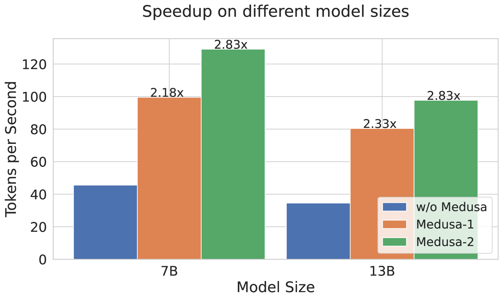
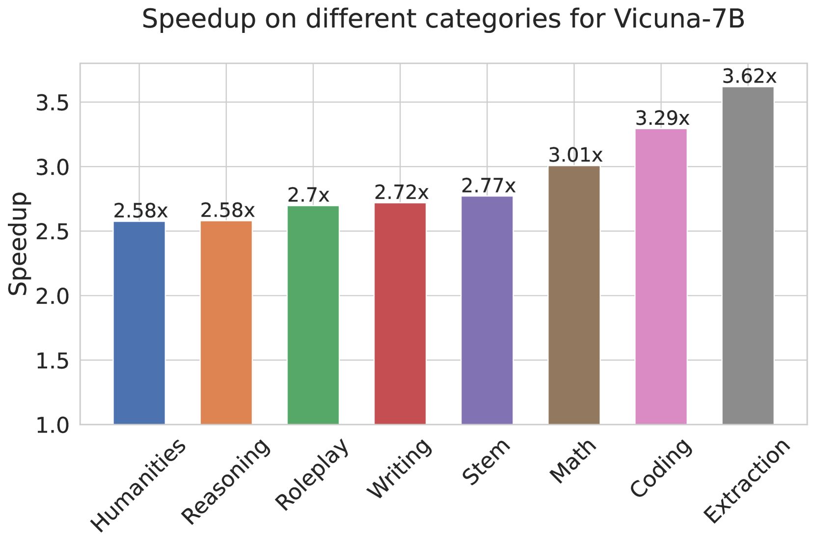
Figure 3: Left: Speed comparison of baseline, Medusa -1 and Medusa -2 on Vicuna-7B/13B. Medusa -1 achieves more than 2 $×$ wall-time speedup compared to the baseline implementation while Medusa -2 further improves the speedup by a significant margin. Right: Detailed speedup performance of Vicuna-7B with Medusa -2 on 8 categories from MT-Bench.
3 Experiments
In this section, we present experiments to demonstrate the effectiveness of Medusa under different settings. First, we evaluate Medusa on the Vicuna-7B and 13B models (Chiang et al., 2023) to show the performance of Medusa -1 and Medusa -2. Then, we assess our method using the Vicuna-33B and Zephyr-7B models to demonstrate self-distillation’s viability in scenarios where direct access to the fine-tuning recipe is unavailable, as with Vicuna-33B, and in models like Zephyr-7B that employ Reinforcement Learning from Human Feedback (RLHF). The evaluation is conducted on MT-Bench (Zheng et al., 2023), a multi-turn, conversational-format benchmark. Detailed settings can be found in Appendix B.
3.1 Case Study: Medusa -1 v.s. Medusa -2 on Vicuna 7B and 13B
Experimental Setup. We use the Vicuna model class (Chiang et al., 2023), which encompasses chat models of varying sizes (7B, 13B, 33B) that are fine-tuned from the Llama model (Touvron et al., 2023). Among them, the 7B and 13B models are trained on the ShareGPT (ShareGPT, 2023) dataset, while the 33B model is an experimental model and is trained on a private dataset. In this section, we use the ShareGPT dataset to train the Medusa heads on the 7B and 13B models for $2$ epochs. We use the v1.5 version of Vicuna models, which are fine-tuned from Llama-2 models with sequence length 4096.
Results. We collect the results and show them in Fig. 3. The baseline is the default Huggingface implementation. In Fig. 3(a), we can see that for the 7B models, Medusa -1 and Medusa -2 configurations lead to a significant increase in speed, measuring in tokens processed per second. Medusa -1 shows a 2.18 $×$ speedup, while Medusa -2 further improves this to a 2.83 $×$ . When applied to the larger 13B model, Medusa -1 results in a 2.33 $×$ speed increase, while Medusa -2 maintains a similar performance gain of 2.83 $×$ over the baseline. We also plot the speedup per category for Medusa -2 Vicuna-7B model. We observe that the coding category benefits from a 3.29 $×$ speedup, suggesting that Medusa is particularly effective for tasks in this domain. This points to a significant potential for optimizing coding LLMs, which are widely used in software development and other programming-related tasks. The “Extraction” category shows the highest speedup at 3.62 $×$ , indicating that this task is highly optimized by the Medusa. Overall, the results suggest that the Medusa significantly enhances inference speed across different model sizes and tasks.
3.2 Case Study: Training with Self-Distillation on Vicuna-33B and Zephyr-7B
Experimental Setup. In this case study, we focus on the cases where self-distillation is needed. We use the Vicuna-33B model (Chiang et al., 2023) and the Zephyr-7B model (Tunstall et al., 2023) as examples. Following the procedure described in Section 2.3.2, we first generate the datasets with some seed prompts. We use ShareGPT (ShareGPT, 2023) and UltraChat (Ding et al., 2023) as the seed datasets and collect a dataset at about $100k$ samples for both cases. Interestingly, we find that the Zephyr model can continue to generate multiple rounds of conversation with a single prompt, which makes it easy to collect a large dataset. For Vicuna-33B, we generate the multi-turn conversations by iteratively feeding the prompts from each multi-turn seed conversation using random sampling with temperature 0.3. Both models are trained with sequence length $2048$ and batch size $128$ .
| Model Name Acc. rate Overhead | Vicuna-7B 3.47 1.22 | Zephyr-7B 3.14 1.18 | Vicuna-13B 3.51 1.23 | Vicuna-33B 3.01 1.27 |
| --- | --- | --- | --- | --- |
| Quality | 6.18 (+0.01) | 7.25 (-0.07) | 6.43 (-0.14) | 7.18 (+0.05) |
| $S_{\textnormal{SpecDecoding}}$ | 1.47 | - | 1.56 | 1.60 |
| $S_{\textsc{Medusa}}$ | 2.83 | 2.66 | 2.83 | 2.35 |
Table 1: Comparison of various Medusa -2 models. The first section reports the details of Medusa -2, including accelerate rate, overhead, and quality that denoted the average scores on the MT-Bench compared to the original models. The second section lists the speedup ( $S$ ) of SpecDecoding and Medusa, respectively.
<details>
<summary>x4.png Details</summary>
### Visual Description
# Technical Document Extraction: Performance Analysis Chart
## 1. Component Isolation
* **Header/Legend:** Located in the top-left quadrant. Contains the label for the primary data series.
* **Main Chart Area:** A scatter plot with an overlaid line graph, featuring a grid background.
* **Axes:** Y-axis (left) representing "Acc. Rate" and X-axis (bottom) representing "Number of Candidate Tokens".
* **Annotations:** Text labels and arrows pointing to specific data points within the plot area.
## 2. Axis and Legend Extraction
### Axis Labels
| Axis | Label | Markers |
| :--- | :--- | :--- |
| **Y-Axis (Vertical)** | `Acc. Rate` | 1.0, 1.5, 2.0, 2.5, 3.0, 3.5 |
| **X-Axis (Horizontal)** | `Number of Candidate Tokens` | 0, 50, 100, 150, 200, 250 |
### Legend
* **Location:** Top-left corner of the plot area.
* **Label:** `Sparse Tree Attention`
* **Visual Style:** Red dashed line with red star markers.
## 3. Data Series Analysis
### Series 1: Sparse Tree Attention (Primary Trend)
* **Visual Trend:** The line slopes upward from left to right, showing a positive correlation between the number of candidate tokens and the acceleration rate. The rate of increase slows down as the x-value increases (logarithmic-like growth).
* **Data Points (Approximate):**
* (64, ~3.15)
* (128, ~3.32)
* (256, ~3.48)
### Series 2: Baseline/Comparison Scatter Plot
* **Visual Trend:** A dense cluster of blue semi-transparent dots. The trend follows a logarithmic curve, starting sharply from x=0 and flattening out as it approaches x=250. The values are consistently lower than the "Sparse Tree Attention" series.
* **Data Range:**
* **X-axis:** Starts near 5 and extends to 256.
* **Y-axis:** Starts near 2.2 and reaches a maximum density around 2.8 - 3.1.
### Series 3: Baseline Marker (w/o Medusa)
* **Visual Trend:** A single isolated data point.
* **Data Point:** (1, 1.0)
* **Annotation:** A grey arrow points from the text "w/o Medusa" to a solid blue circle at the coordinate (1, 1.0).
## 4. Summary of Findings
The chart illustrates the performance improvement (Acceleration Rate) of different configurations based on the number of candidate tokens used.
1. **Baseline (w/o Medusa):** Represents the starting point with an Acc. Rate of 1.0 at 1 candidate token.
2. **Standard Medusa (Scatter Plot):** Shows significant improvement over the baseline, reaching Acc. Rates between 2.5 and 3.0 as candidate tokens increase.
3. **Sparse Tree Attention (Red Dashed Line):** Represents the highest performing method shown. It consistently outperforms the standard scatter plot data points. At 256 candidate tokens, it achieves an acceleration rate of approximately 3.5x, compared to the ~3.0x seen in the dense scatter plot.
</details>
(a)
<details>
<summary>x5.png Details</summary>
### Visual Description
# Technical Document Extraction: Performance Analysis of Sparse Tree Attention
## 1. Image Overview
This image is a scatter plot with an overlaid line graph comparing the inference speed (throughput) of different configurations for a Large Language Model (LLM) acceleration technique, likely related to the "Medusa" speculative decoding framework.
## 2. Component Isolation
### Header / Metadata
* **Language:** English
* **Primary Subject:** Speed (token/s) vs. Number of Candidate Tokens.
### Axis Definitions
* **Y-Axis (Vertical):**
* **Label:** Speed (token/s)
* **Scale:** Linear, ranging from 60 to 120 with major tick marks every 20 units (60, 80, 100, 120).
* **X-Axis (Horizontal):**
* **Label:** Number of Candidate Tokens
* **Scale:** Linear, ranging from 0 to 250 with major tick marks every 50 units (0, 50, 100, 150, 200, 250).
### Legend [Spatial Placement: Top Right]
| Symbol | Label |
| :--- | :--- |
| Red dashed line with star markers (`--*--`) | Sparse Tree Attention |
## 3. Data Series Analysis
### Series 1: Baseline (w/o Medusa)
* **Visual Description:** A single blue circular data point located at the bottom left of the chart.
* **Annotation:** An arrow points to this dot with the text "w/o Medusa".
* **Coordinates:** Approximately [x: 1, y: 45].
* **Trend:** This represents the base performance of the model without speculative decoding enhancements.
### Series 2: Standard Medusa / Dense Attention (Scatter Plot)
* **Visual Description:** A dense collection of small blue semi-transparent dots.
* **Trend Verification:**
* **0 to 60 tokens:** The speed increases sharply as the number of candidate tokens increases, peaking around 110 token/s.
* **60 to 250 tokens:** The speed follows a "stair-step" downward trend. There are distinct clusters where performance drops significantly at specific thresholds (roughly at 128 and 192 tokens).
* **Key Data Clusters:**
* **Peak:** ~110 token/s at ~60 candidate tokens.
* **Mid-range:** ~100 token/s between 70 and 125 candidate tokens.
* **Lower-range:** ~85 token/s between 130 and 185 candidate tokens.
* **Bottom-range:** ~75 token/s between 190 and 250 candidate tokens.
### Series 3: Sparse Tree Attention (Line Graph)
* **Visual Description:** A red dashed line connecting three large red star markers.
* **Trend Verification:** The line slopes downward as the number of candidate tokens increases, but it consistently maintains a higher speed than the blue scatter points (Standard Medusa).
* **Extracted Data Points:**
1. **Point 1:** [x: ~64, y: ~118] - Highest recorded speed.
2. **Point 2:** [x: ~128, y: ~112] - Maintains high speed even as candidate tokens double.
3. **Point 3:** [x: ~256, y: ~82] - Speed drops as candidate tokens reach the maximum shown, but remains above the dense scatter plot baseline for that x-value.
## 4. Technical Summary and Findings
* **Performance Gain:** Implementing Medusa (even without Sparse Tree Attention) provides a massive speedup from ~45 token/s to over 100 token/s.
* **Efficiency Optimization:** "Sparse Tree Attention" (Red Line) acts as a Pareto frontier, representing the optimal speed for a given number of candidate tokens. It effectively mitigates the performance degradation seen in the standard implementation (Blue Dots) as the complexity (number of tokens) increases.
* **Scaling Behavior:** Standard attention shows significant performance "cliffs" or drops at specific token counts, likely due to hardware memory limits or kernel inefficiencies. Sparse Tree Attention smooths this degradation and keeps the throughput significantly higher at high candidate counts (e.g., at 250 tokens, Sparse Tree is ~82 token/s vs ~75 token/s for standard).
</details>
(b)
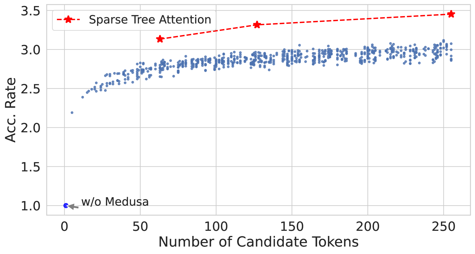
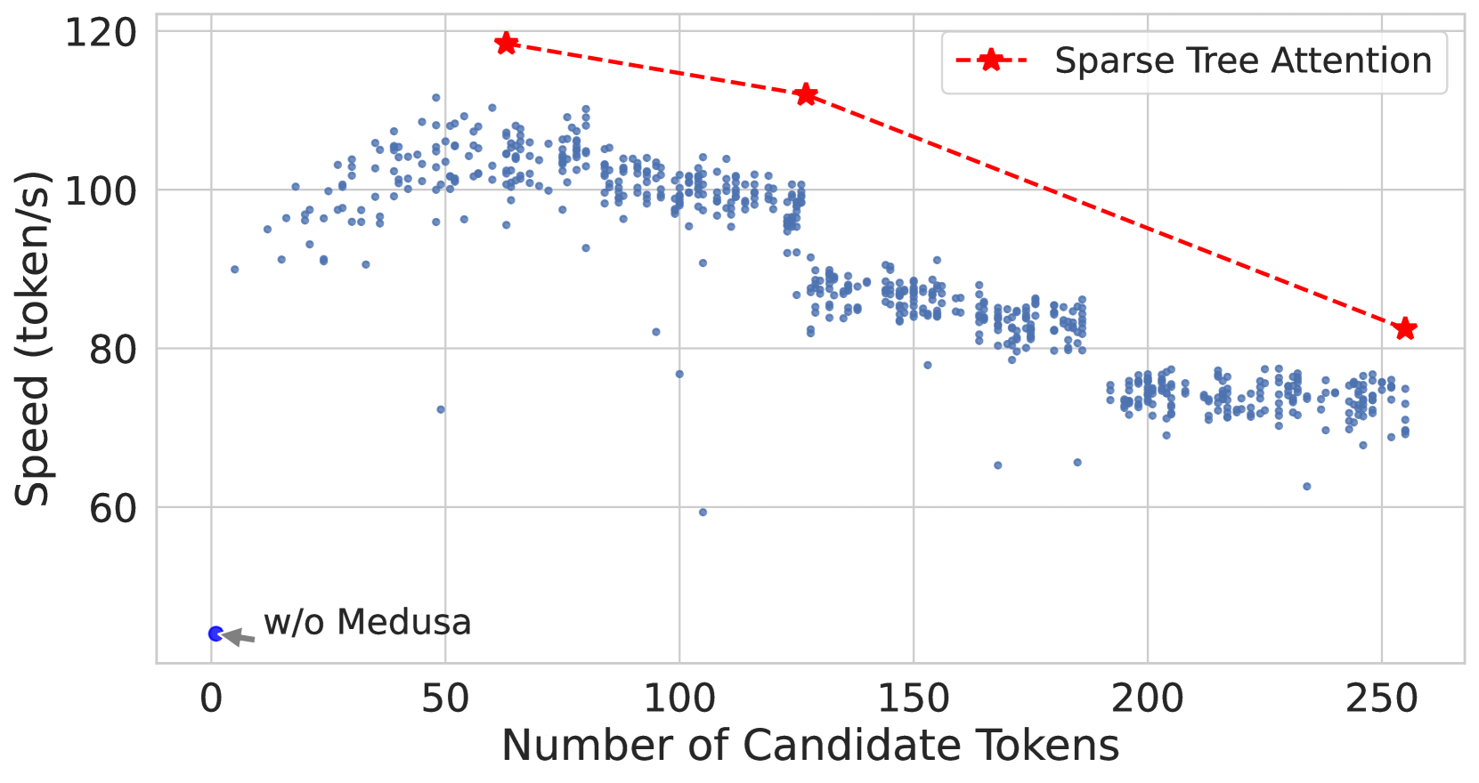
Figure 4: Effectiveness of numbers of candidate tokens for decoding introduced by trees (default number of candidate token for decoding is 1 when using KV cache). Left: The acceleration rate for randomly sampled dense tree settings (blue dots) and optimized sparse tree settings (red stars). Right: The speed (tokens/s) for both settings. The trend lines indicate that while the acceleration rate remains relatively stable for sparse trees, there is a notable decrease in speed as the candidate tokens increases.
Results. Table 1 complements these findings by comparing various Medusa -2 models in terms of their acceleration rate, overhead, and quality on MT-Bench with GPT-4 acting as the evaluator to assign performance scores ranging from 0 to 10. We report the quality differences of Medusa compared to the original model. Notably, while the Medusa -2 Vicuna-33B model shows a lower acceleration rate, it maintains a comparable quality. We hypothesize that this is due to a mismatch between the hidden training dataset and the dataset we used for self-distillation. Hence, the model’s generation quality can be well aligned by self-distillation while Medusa heads learn distribution from the self-distillation that potentially shifts from the training set. In our study, we also applied speculative decoding (Chen et al., 2023; Leviathan et al., 2022) to the Vicuna lineup using open-source draft models (details can be found in Appendix D).
These results underscore the complex interplay between speed and performance when scaling up model sizes and applying self-distillation techniques. The findings also highlight the potential of the Medusa -2 configuration to boost efficiency in processing while carefully preserving the quality of the model’s outputs, suggesting a promising direction for co-optimizing LLMs with Medusa heads.
3.3 Ablation Study
3.3.1 Configuration of Tree Attention
The study of tree attention is conducted on the writing and roleplay categories from the MT-Bench dataset using Medusa -2 Vicuna-7B. We target to depict tree attention’s motivation and its performance.
Fig. 4(a) compares the acceleration rate of randomly sampled dense tree configurations (Section. 2.1.2, depicted by blue dots) against optimized sparse tree settings (Section. 2.3.3, shown with red stars). The sparse tree configuration with 64 nodes shows a better acceleration rate than the dense tree settings with 256 nodes. The decline in speed in Fig. 4(b) is attributed to the increased overhead introduced by the compute-bound. While a more complex tree can improve acceleration, it does so at the cost of speed due to intensive matrix multiplications for linear layers and self-attention. The acceleration rate increase follows a logarithmic trend and slows down when the tree size grows as shown in Fig. 4(a). However, the initial gains are substantial, allowing Medusa to achieve significant speedups. If the acceleration increase is less than the overhead, it will slow down overall performance. For detailed study, please refer to Appendix G.
<details>
<summary>x6.png Details</summary>
### Visual Description
# Technical Document Extraction: Performance Metrics vs. Posterior Thresholds
## 1. Image Overview
This image is a dual-axis line chart comparing two performance metrics—**Acc. Rate** (Acceptance Rate) and **Scores**—across a range of **Posterior Thresholds**. The chart also includes baseline markers for two methodologies: **RS** (Random Search) and **Greedy**.
## 2. Component Isolation
### A. Header / Metadata
* **Language:** English.
* **Content:** No explicit title text is present above the chart area.
### B. Main Chart Area (Axes and Labels)
* **X-Axis (Bottom):**
* **Label:** `Posterior Thresholds`
* **Scale:** Linear, ranging from `0.00` to `0.25`.
* **Markers:** `0.00`, `0.05`, `0.10`, `0.15`, `0.20`, `0.25`.
* **Primary Y-Axis (Left - Blue):**
* **Label:** `Acc. Rate`
* **Scale:** Linear, ranging from `3.0` to `3.5`.
* **Markers:** `3.0`, `3.1`, `3.2`, `3.3`, `3.4`, `3.5`.
* **Secondary Y-Axis (Right - Orange/Gold):**
* **Label:** `Scores`
* **Scale:** Linear, ranging from `7.0` to `7.6`.
* **Markers:** `7.0`, `7.1`, `7.2`, `7.3`, `7.4`, `7.5`, `7.6`.
### C. Legend and Baselines
The chart utilizes a non-standard legend format where baseline values are plotted as individual points on the Y-axes.
* **Left Side Baselines (Acc. Rate):**
* **Greedy (Blue Star):** Positioned at approximately `Acc. Rate = 3.05` at `Threshold = 0.00`.
* **RS (Blue Circle):** Positioned at approximately `Acc. Rate = 2.98` (just below the 3.0 line) at `Threshold = 0.00`.
* **Right Side Baselines (Scores):**
* **RS (Orange Circle):** Positioned at approximately `Score = 7.45`.
* **Greedy (Orange Star):** Positioned at approximately `Score = 7.41`.
---
## 3. Data Series Analysis
### Series 1: Acc. Rate (Solid Blue Line)
* **Trend Verification:** The line starts at its maximum value and exhibits a sharp downward slope initially. After reaching a local minimum around threshold 0.06, it enters a stabilized oscillatory pattern (a "wavy" horizontal trend) for the remainder of the x-axis.
* **Key Data Points:**
* **Start (0.01):** ~3.50 (Peak)
* **Initial Drop (0.05):** ~3.30
* **Local Min (0.06):** ~3.24
* **Stabilization Range:** Fluctuates between ~3.22 and ~3.30 for thresholds 0.07 to 0.25.
* **End (0.25):** ~3.26
### Series 2: Scores (Solid Orange/Gold Line)
* **Trend Verification:** This series is highly volatile. It shows no singular upward or downward trend but rather a series of sharp peaks and valleys across the entire threshold range.
* **Key Data Points:**
* **Start (0.01):** ~7.05
* **First Peak (0.06):** ~7.38
* **Deep Valley (0.10):** ~7.02
* **Mid Peak (0.14):** ~7.42
* **Deep Valley (0.16):** ~7.08
* **High Peak (0.20):** ~7.55
* **Final Peak (0.24):** ~7.58 (Global Maximum)
* **End (0.25):** ~7.52
---
## 4. Summary of Findings
1. **Inverse Relationship (Initial):** At very low posterior thresholds (< 0.05), the Acceptance Rate is at its highest while Scores are relatively low.
2. **Stability vs. Volatility:** The `Acc. Rate` (Blue) becomes relatively stable after the initial threshold increase, whereas the `Scores` (Orange) remain highly sensitive to specific threshold values, showing significant variance.
3. **Baseline Comparison:**
* The `Acc. Rate` for all thresholds shown (0.01 - 0.25) remains significantly higher than the **Greedy** (~3.05) and **RS** (~2.98) baselines.
* The `Scores` fluctuate around the **RS** (~7.45) and **Greedy** (~7.41) baselines, only consistently exceeding them at specific threshold intervals (e.g., near 0.20 and 0.24).
</details>
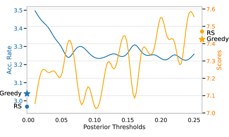
Figure 5: Performance comparison of Medusa using proposed typical sampling. The model is fully fine-tuned from Vicuna-7B. The plot illustrates the acceleration rate and average scores on the writing and roleplay (MT-Bench) with a fixed temperature of 0.7 for 3 different settings: greedy sampling and random sampling (RS) plotted as the star and the dot, and typical sampling curves under different thresholds.
3.3.2 Thresholds of Typical Acceptance
The thresholds of typical acceptance are studied on the writing and roleplay categories from the MT-Bench dataset (Zheng et al., 2023) using Medusa -2 Vicuna 7B. Utilizing the Vicuna 7B model, we aligned our methodology with the approach delineated by (Hewitt et al., 2022) setting the $\alpha=\sqrt{\epsilon}$ . Fig. 5 presents a comparative analysis of our model’s performance across various sampling settings. These settings range from a threshold $\epsilon$ starting at 0.01 and incrementally increasing to 0.25 in steps of 0.01. Our observations indicate a discernible trade-off: as $\epsilon$ increases, there is an elevation in quality at the expense of a reduced acceleration rate. Furthermore, for tasks demanding creativity, it is noted that the default random sampling surpasses greedy sampling in performance, and the proposed typical sampling is comparable with random sampling when $\epsilon$ increases.
| | Baseline | Direct Fine-tuning | Medusa -1 | Medusa -2 |
| --- | --- | --- | --- | --- |
| Quality | 6.17 | 5.925 | 6.23 | 6.18 |
| Speedup | N/A | N/A | 2.18 | 2.83 |
Table 2: Comparison of Different Settings of Vicuna-7B. Quality is obtained by evaluating models on MT-Bench using GPT-4 as the judge (higher the better).
3.3.3 Effectiveness of Two-stage Fine-tuning
Table 2 shows the performance differences between various fine-tuning strategies for the Vicuna-7B model. Medusa -1, which fine-tunes only the Medusa heads, achieves a 2.18x speedup without compromising generation quality. Medusa -2, which employs two-stage fine-tuning (Section 2.2.2), maintains generation quality and provides greater speedup (2.83x) compared to Medusa -1. In contrast, direct fine-tuning the model with the Medusa heads results in degraded generation quality. The findings indicate that implementing our Medusa -2 for fine-tuning maintains the model’s quality and concurrently improves the speedup versus Medusa -1.
Table 3: Impact of Techniques on Speedup
| Medusa-1 heads without tree attention | $\sim$ 1.5x |
| --- | --- |
| Adding tree attention | $\sim$ 1.9x |
| Using optimized tree configuration | $\sim$ 2.2x |
| Training heads with Medusa-2 | $\sim$ 2.8x |
4 Discussion
In conclusion, Medusa enhances LLM inference speed by 2.3-2.8 times by equipping models with additional predictive decoding heads, allowing for generating multiple tokens simultaneously and bypassing the sequential decoding limitation. Key advantages of Medusa include its simplicity, parameter efficiency, and ease of integration into existing systems. Medusa avoids the need for specialized draft models. The typical acceptance scheme removes complications from rejection sampling while providing reasonable outputs. Our approach including two efficient training procedures, ensures high-quality output across various models and prompt types. We summarize the development of each technique and their impact on the speedup in Table 3.
In the paper, we focus on the setting with batch size 1 for simplicity. Yet, we want to emphasize that the ideas presented in our paper can be generalized to larger batch-size settings, which are now supported by libraries like TensorRT and Huggingface TGI following our paper.
Acknowledgements
We extend our heartfelt gratitude to several individuals whose contributions were invaluable to this project:
- Zhuohan Li, for his invaluable insights on LLM serving. If you haven’t already, do check out Zhuohan’s vLLM project—it’s nothing short of impressive.
- Shaojie Bai, for engaging in crucial discussions that helped shape the early phases of this work.
- Denny Zhou, for introducing the truncation sampling scheme to Tianle and encouraging Tianle to explore the area of LLM serving.
- Yanping Huang, for pointing out the memory-bandwidth-bound challenges associated with LLM serving to Tianle.
- Lianmin Zheng, for clarifying the different training recipes used in different sizes of Vicuna models.
Jason D. Lee acknowledges the support of the NSF CCF 2002272, NSF IIS 2107304, and NSF CAREER Award 2144994. Deming Chen acknowledges the support from the AMD Center of Excellence at UIUC.
Impact Statement
The introduction of Medusa, an innovative method to improve the inference speed of Large Language Models (LLMs), presents a range of broader implications for society, technology, and ethics. This section explores these implications in detail.
Societal and Technological Implications
- Accessibility and Democratization of AI: By significantly enhancing the efficiency of LLMs, Medusa makes advanced AI technologies more accessible to a wider range of users and organizations. Democratization can spur innovation across various sectors, including education, healthcare, and entertainment, potentially leading to breakthroughs that benefit society at large.
- Environmental Impact: The acceleration for LLM inference due to Medusa could lead to decreased energy consumption and a smaller carbon footprint. This aligns with the growing need for sustainable AI practices, contributing to environmental conservation efforts.
- Economic Implications: The increased efficiency brought about by Medusa may lower the cost barrier to deploying state-of-the-art AI models, enabling small and medium-sized enterprises to leverage advanced AI capabilities. This could stimulate economic growth, foster competition, and drive technological innovation.
Ethical Considerations
- Bias and Fairness: While Medusa aims to improve LLM efficiency, it inherits the ethical considerations of its backbone models, including issues related to bias and fairness. The method’s ability to maintain generation quality necessitates investigation to ensure that the models do not perpetuate or amplify existing biases.
- Transparency and Accountability: The complexity of Medusa, particularly with its tree-based attention mechanism and multiple decoding heads, may pose challenges in terms of model interpretability. Ensuring transparency in how decisions are made and maintaining accountability for those decisions are crucial for building trust in AI systems.
- Security and Privacy: The accelerated capabilities of LLMs augmented by Medusa could potentially be exploited for malicious purposes, such as generating disinformation at scale or automating cyber-attacks. It is imperative to develop and enforce ethical guidelines and security measures to prevent misuse.
References
- Ainslie et al. (2023) Ainslie, J., Lee-Thorp, J., de Jong, M., Zemlyanskiy, Y., Lebrón, F., and Sanghai, S. Gqa: Training generalized multi-query transformer models from multi-head checkpoints. arXiv preprint arXiv:2305.13245, 2023.
- Axolotl (2023) Axolotl. Axolotl. https://github.com/OpenAccess-AI-Collective/axolotl, 2023.
- Basu et al. (2021) Basu, S., Ramachandran, G. S., Keskar, N. S., and Varshney, L. R. {MIROSTAT}: A {neural} {text} {decoding} {algorithm} {that} {directly} {controls} {perplexity}. In International Conference on Learning Representations, 2021. URL https://openreview.net/forum?id=W1G1JZEIy5_.
- Brown et al. (2020) Brown, T., Mann, B., Ryder, N., Subbiah, M., Kaplan, J. D., Dhariwal, P., Neelakantan, A., Shyam, P., Sastry, G., Askell, A., et al. Language models are few-shot learners. Advances in neural information processing systems, 33:1877–1901, 2020.
- Chen et al. (2023) Chen, C., Borgeaud, S., Irving, G., Lespiau, J.-B., Sifre, L., and Jumper, J. Accelerating large language model decoding with speculative sampling. February 2023. doi: 10.48550/ARXIV.2302.01318.
- Chen (2023) Chen, L. Dissecting batching effects in gpt inference. https://le.qun.ch/en/blog/2023/05/13/transformer-batching/, 2023. Blog.
- Chiang et al. (2023) Chiang, W.-L., Li, Z., Lin, Z., Sheng, Y., Wu, Z., Zhang, H., Zheng, L., Zhuang, S., Zhuang, Y., Gonzalez, J. E., Stoica, I., and Xing, E. P. Vicuna: An open-source chatbot impressing gpt-4 with 90%* chatgpt quality, March 2023. URL https://lmsys.org/blog/2023-03-30-vicuna/.
- Chowdhery et al. (2022) Chowdhery, A., Narang, S., Devlin, J., Bosma, M., Mishra, G., Roberts, A., Barham, P., Chung, H. W., Sutton, C., Gehrmann, S., et al. Palm: Scaling language modeling with pathways. arXiv preprint arXiv:2204.02311, 2022.
- Dettmers et al. (2021) Dettmers, T., Lewis, M., Shleifer, S., and Zettlemoyer, L. 8-bit optimizers via block-wise quantization. International Conference on Learning Representations, 2021.
- Dettmers et al. (2022) Dettmers, T., Lewis, M., Belkada, Y., and Zettlemoyer, L. Llm. int8 (): 8-bit matrix multiplication for transformers at scale. arXiv preprint arXiv:2208.07339, 2022.
- Dettmers et al. (2023) Dettmers, T., Pagnoni, A., Holtzman, A., and Zettlemoyer, L. Qlora: Efficient finetuning of quantized llms. arXiv preprint arXiv:2305.14314, 2023.
- Ding et al. (2023) Ding, N., Chen, Y., Xu, B., Qin, Y., Zheng, Z., Hu, S., Liu, Z., Sun, M., and Zhou, B. Enhancing chat language models by scaling high-quality instructional conversations, 2023.
- Dubois et al. (2023) Dubois, Y., Li, X., Taori, R., Zhang, T., Gulrajani, I., Ba, J., Guestrin, C., Liang, P., and Hashimoto, T. B. Alpacafarm: A simulation framework for methods that learn from human feedback, 2023.
- Elfwing et al. (2017) Elfwing, S., Uchibe, E., and Doya, K. Sigmoid-weighted linear units for neural network function approximation in reinforcement learning. Neural Networks, 2017. doi: 10.1016/j.neunet.2017.12.012.
- Fan et al. (2018) Fan, A., Lewis, M., and Dauphin, Y. Hierarchical neural story generation. In Proceedings of the 56th Annual Meeting of the Association for Computational Linguistics (Volume 1: Long Papers). Association for Computational Linguistics, 2018. doi: 10.18653/v1/p18-1082.
- Frantar et al. (2022) Frantar, E., Ashkboos, S., Hoefler, T., and Alistarh, D. Gptq: Accurate post-training quantization for generative pre-trained transformers. arXiv preprint arXiv:2210.17323, 2022.
- Google (2023) Google. Palm 2 technical report, 2023. URL https://ai.google/static/documents/palm2techreport.pdf.
- Hewitt et al. (2022) Hewitt, J., Manning, C. D., and Liang, P. Truncation sampling as language model desmoothing. October 2022. doi: 10.48550/ARXIV.2210.15191.
- Hoffmann et al. (2022) Hoffmann, J., Borgeaud, S., Mensch, A., Buchatskaya, E., Cai, T., Rutherford, E., Casas, D. d. L., Hendricks, L. A., Welbl, J., Clark, A., et al. Training compute-optimal large language models. arXiv preprint arXiv:2203.15556, 2022.
- Holtzman et al. (2020) Holtzman, A., Buys, J., Du, L., Forbes, M., and Choi, Y. The curious case of neural text degeneration. In International Conference on Learning Representations, 2020. URL https://openreview.net/forum?id=rygGQyrFvH.
- Hu et al. (2021) Hu, E. J., Shen, Y., Wallis, P., Allen-Zhu, Z., Li, Y., Wang, S., and Chen, W. Lora: Low-rank adaptation of large language models. ICLR, 2021.
- Joao Gante (2023) Joao Gante. Assisted generation: a new direction toward low-latency text generation, 2023. URL https://huggingface.co/blog/assisted-generation.
- Kim et al. (2023) Kim, S., Hooper, C., Gholami, A., Dong, Z., Li, X., Shen, S., Mahoney, M. W., and Keutzer, K. Squeezellm: Dense-and-sparse quantization. arXiv preprint arXiv:2306.07629, 2023.
- Kim & Rush (2016) Kim, Y. and Rush, A. M. Sequence-level knowledge distillation. EMNLP, 2016.
- Kumar et al. (2022) Kumar, A., Raghunathan, A., Jones, R., Ma, T., and Liang, P. Fine-tuning can distort pretrained features and underperform out-of-distribution. International Conference on Learning Representations, 2022.
- Kwon et al. (2023) Kwon, W., Li, Z., Zhuang, S., Sheng, Y., Zheng, L., Yu, C. H., Gonzalez, J. E., Zhang, H., and Stoica, I. Efficient memory management for large language model serving with pagedattention. In Proceedings of the ACM SIGOPS 29th Symposium on Operating Systems Principles, 2023.
- Leviathan et al. (2022) Leviathan, Y., Kalman, M., and Matias, Y. Fast inference from transformers via speculative decoding. November 2022. doi: 10.48550/ARXIV.2211.17192.
- Li et al. (2023) Li, X., Zhang, T., Dubois, Y., Taori, R., Gulrajani, I., Guestrin, C., Liang, P., and Hashimoto, T. B. Alpacaeval: An automatic evaluator of instruction-following models. https://github.com/tatsu-lab/alpaca_eval, 2023.
- Lin et al. (2023) Lin, J., Tang, J., Tang, H., Yang, S., Dang, X., and Han, S. Awq: Activation-aware weight quantization for llm compression and acceleration. arXiv preprint arXiv:2306.00978, 2023.
- Meister et al. (2022) Meister, C., Wiher, G., Pimentel, T., and Cotterell, R. On the probability-quality paradox in language generation. March 2022. doi: 10.48550/ARXIV.2203.17217.
- Meister et al. (2023) Meister, C., Pimentel, T., Wiher, G., and Cotterell, R. Locally typical sampling. Transactions of the Association for Computational Linguistics, 11:102–121, 2023.
- Miao et al. (2023) Miao, X., Oliaro, G., Zhang, Z., Cheng, X., Wang, Z., Wong, R. Y. Y., Chen, Z., Arfeen, D., Abhyankar, R., and Jia, Z. Specinfer: Accelerating generative llm serving with speculative inference and token tree verification. arXiv preprint arXiv:2305.09781, 2023.
- (33) NVIDIA. Nvidia a100 tensor core gpu.
- OpenAI (2023) OpenAI. Gpt-4 technical report, 2023.
- Ouyang et al. (2022) Ouyang, L., Wu, J., Jiang, X., Almeida, D., Wainwright, C. L., Mishkin, P., Zhang, C., Agarwal, S., Slama, K., Ray, A., et al. Training language models to follow instructions with human feedback. arXiv preprint arXiv:2203.02155, 2022.
- Pan (2023) Pan, J. Tiny vicuna 1b. https://huggingface.co/Jiayi-Pan/Tiny-Vicuna-1B, 2023.
- Pillutla et al. (2021) Pillutla, K., Swayamdipta, S., Zellers, R., Thickstun, J., Welleck, S., Choi, Y., and Harchaoui, Z. MAUVE: Measuring the gap between neural text and human text using divergence frontiers. In Beygelzimer, A., Dauphin, Y., Liang, P., and Vaughan, J. W. (eds.), Advances in Neural Information Processing Systems, 2021. URL https://openreview.net/forum?id=Tqx7nJp7PR.
- Pope et al. (2022) Pope, R., Douglas, S., Chowdhery, A., Devlin, J., Bradbury, J., Levskaya, A., Heek, J., Xiao, K., Agrawal, S., and Dean, J. Efficiently scaling transformer inference. November 2022. doi: 10.48550/ARXIV.2211.05102.
- ShareGPT (2023) ShareGPT. ShareGPT. https://huggingface.co/datasets/Aeala/ShareGPT_Vicuna_unfiltered, 2023.
- Shazeer (2019) Shazeer, N. Fast transformer decoding: One write-head is all you need. arXiv preprint arXiv:1911.02150, 2019.
- Spector & Re (2023) Spector, B. and Re, C. Accelerating llm inference with staged speculative decoding. arXiv preprint arXiv:2308.04623, 2023.
- Stern et al. (2018) Stern, M., Shazeer, N. M., and Uszkoreit, J. Blockwise parallel decoding for deep autoregressive models. Neural Information Processing Systems, 2018.
- Touvron et al. (2023) Touvron, H., Martin, L., Stone, K., Albert, P., Almahairi, A., Babaei, Y., Bashlykov, N., Batra, S., Bhargava, P., Bhosale, S., et al. Llama 2: Open foundation and fine-tuned chat models. arXiv preprint arXiv:2307.09288, 2023.
- Tunstall et al. (2023) Tunstall, L., Beeching, E., Lambert, N., Rajani, N., Rasul, K., Belkada, Y., Huang, S., von Werra, L., Fourrier, C., Habib, N., Sarrazin, N., Sanseviero, O., Rush, A. M., and Wolf, T. Zephyr: Direct distillation of lm alignment, 2023.
- Xia et al. (2023) Xia, H., Ge, T., Chen, S.-Q., Wei, F., and Sui, Z. Speculative decoding: Lossless speedup of autoregressive translation, 2023. URL https://openreview.net/forum?id=H-VlwsYvVi.
- Xiao et al. (2023a) Xiao, G., Lin, J., Seznec, M., Wu, H., Demouth, J., and Han, S. Smoothquant: Accurate and efficient post-training quantization for large language models. In International Conference on Machine Learning, pp. 38087–38099. PMLR, 2023a.
- Xiao et al. (2023b) Xiao, Y., Wu, L., Guo, J., Li, J., Zhang, M., Qin, T., and Liu, T.-y. A survey on non-autoregressive generation for neural machine translation and beyond. IEEE Transactions on Pattern Analysis and Machine Intelligence, 2023b.
- Ying et al. (2021) Ying, C., Cai, T., Luo, S., Zheng, S., Ke, G., He, D., Shen, Y., and Liu, T.-Y. Do transformers really perform badly for graph representation? Advances in Neural Information Processing Systems, 34:28877–28888, 2021.
- Zhang et al. (2024) Zhang, P., Zeng, G., Wang, T., and Lu, W. Tinyllama: An open-source small language model, 2024.
- Zhang et al. (2022) Zhang, S., Roller, S., Goyal, N., Artetxe, M., Chen, M., Chen, S., Dewan, C., Diab, M., Li, X., Lin, X. V., et al. Opt: Open pre-trained transformer language models. arXiv preprint arXiv:2205.01068, 2022.
- Zhang et al. (2023) Zhang, Z., Sheng, Y., Zhou, T., Chen, T., Zheng, L., Cai, R., Song, Z., Tian, Y., Ré, C., Barrett, C., et al. H $\_2$ o: Heavy-hitter oracle for efficient generative inference of large language models. arXiv preprint arXiv:2306.14048, 2023.
- Zheng et al. (2023) Zheng, L., Chiang, W.-L., Sheng, Y., Zhuang, S., Wu, Z., Zhuang, Y., Lin, Z., Li, Z., Li, D., Xing, E. P., Zhang, H., Gonzalez, J. E., and Stoica, I. Judging llm-as-a-judge with mt-bench and chatbot arena, 2023.
Appendix A Related Work
A.1 LLM Inference Acceleration
The inefficiency of Large Language Model (LLM) inference is primarily attributed to the memory-bandwidth-bound nature of the auto-regressive decoding process. Several methods have been proposed to alleviate this issue, improving inference latency and throughput. Traditionally, batch inference has been employed as a straightforward method to enhance arithmetic intensity and escape memory-bandwidth-bound limitations. However, with LLMs, both model parameters and the Key-Value (KV) cache consume substantial accelerator memory, hindering the utilization of large batch sizes. Existing methods to tackle this problem can be conceptually divided into two main categories: (1) Reducing memory consumption, thereby minimizing memory transfer overhead and enabling larger batch sizes, and (2) Minimizing the number of decoding steps to decrease latency directly.
Reducing KV Cache.
Methods such as Multi-query attention (Shazeer, 2019) and Grouped-query attention (Ainslie et al., 2023) adopt a direct approach to diminish the KV cache. By utilizing fewer key and value heads in the attention modules relative to query heads, these strategies substantially cut the KV’s memory consumption, thereby facilitating larger batch sizes and enhanced accelerator utilization (Pope et al., 2022). Additionally, Zhang et al. (2023) proposes to selectively retain the most critical KV tokens, further reducing the KV cache. From a system perspective, Kwon et al. (2023) introduces a paged memory management scheme for reducing fragmentation of the KV cache.
Quantization.
Quantization techniques are extensively used to shrink LLMs’ memory consumption. Xiao et al. (2023a) apply rescaling between activations and parameters to eliminate outliers and simplify the quantization process. Dettmers et al. (2022) breaks down matrix multiplications into predominantly 8-bit and a minority of 16-bit operations. Frantar et al. (2022) iteratively round weight columns into 3/4 bits, while Lin et al. (2023) present an activation-aware quantization scheme to protect salient weights and compress LLMs to 3/4 bits. Kim et al. (2023) introduce a sparse plus low-precision pattern to handle a minor portion of vital weights, among other techniques.
Speculative Decoding.
As an approach orthogonal to the aforementioned methods, speculative decoding (Leviathan et al., 2022; Chen et al., 2023) aims to execute several decoding steps in parallel, thus reducing the total number of steps required. This parallelization is realized by employing a smaller draft model to conjecture several subsequent words, which the LLMs then collectively evaluate and accept as appropriate. While resonating with non-autoregressive generation literature (Xiao et al., 2023b), this method is specifically tailored for LLMs to address the aforementioned inefficiency. Unlike previous works, we propose leveraging the original model to make predictions rather than introducing an additional draft model. This approach is more straightforward and seamlessly integrates into existing systems without the complexities of managing two models. Independently, Miao et al. (2023); Spector & Re (2023) propose the use of tree-structured attention to generate multiple candidates in parallel, where Miao et al. (2023) suggest employing an ensemble of models to propose candidates, and Spector & Re (2023) advocate adding another hierarchy for the draft model. However, draft models require specialized pretraining and alignment with the target models. While employing multiple draft models can be cumbersome and involves the complexity of managing parallelism, our approach, which relies solely on decoding heads, offers a simpler alternative. Miao et al. (2023) employ multiple draft models to generate tokens and merge them using tree attention, while Spector & Re (2023) utilize a small draft model to process each level of the tree in batches. In contrast, our method directly uses the top predicted tokens from each of Medusa heads to create a static sparse tree without autoregression or adjusting the tree structure. This approach simplifies the process and improves efficiency. Additionally, we demonstrate through a detailed ablation study how the nodes of the tree can affect decoding speed.
A.2 Sampling Scheme
The manner in which text is sampled from Large Language Models (LLMs) can significantly influence the quality of the generated output. Recent studies have revealed that direct sampling from a language model may lead to incoherent or nonsensical results (Pillutla et al., 2021; Holtzman et al., 2020). In response to this challenge, truncation sampling schemes have been introduced (Fan et al., 2018; Basu et al., 2021; Meister et al., 2022; Hewitt et al., 2022; Meister et al., 2023). These approaches aim to produce high-quality and diverse samples by performing sampling on a truncated distribution over a specific allowed set at each decoding step.
Different strategies define this allowed set in various ways. For example, top- $k$ sampling (Fan et al., 2018) retains the $k$ most likely words, whereas top- $p$ sampling (Holtzman et al., 2020) incorporates the minimal set of words that account for $p$ percent of the probability. Another method, known as typical decoding (Meister et al., 2023), employs the entropy of the predicted distribution to establish the threshold for inclusion. Hewitt et al. (2022) offers a unified framework to understand truncation sampling techniques comprehensively.
Drawing inspiration from these methods, our typical acceptance scheme aligns with the concept of defining an allowed set to exclude improbable candidates from the sampling process. However, we diverge because we do not insist on an exact correspondence between the output and language model distribution. This deviation allows us to facilitate more diverse yet high-quality outputs, achieving greater efficiency without compromising the integrity of the generated text.
Appendix B Experiment Settings
B.1 Common Terms
We clarify three commonly used terms: a) Acceleration rate: This refers to the average number of tokens decoded per decoding step. In a standard auto-regressive model, this rate is 1.0. b) Overhead: This is used to characterize the per decoding step overhead compared to classic decoding, and is calculated by dividing the average per step latency of the Medusa models by that of the vanilla model. c) Speedup: This refers to the wall-time acceleration rate. Following these definitions, we have the relation: Speedup = Acceleration rate / Overhead.
B.2 Shared Settings
For all the experiments, we use the Axolotl (Axolotl, 2023) framework for training. We use a cosine learning rate scheduler with warmup and use 8-bit AdamW (Dettmers et al., 2021) optimizer. We train $5$ Medusa heads with $1$ layer and set $\lambda_{k}$ in Eq. (1) to be $0.8^{k}$ . For Medusa -2, we use either LoRA (Hu et al., 2021) or QLoRA (Dettmers et al., 2023) for fine-tuning and set the learning rate of Medusa heads to be $4$ times larger than the backbone model. LoRA is applied to all the linear layers of the backbone model, including the language model head. The rank of LoRA adapter is set to $32$ , and $\alpha$ is set to $16$ . A dropout of $0.05$ is added to the LoRA adapter.
B.3 Medusa -1 v.s. Medusa -2 on Vicuna 7B and 13B
We use a global batch size of $64$ and a peak learning rate of $5e^{-4}$ for the backbone and $2e^{-3}$ for Medusa heads and warmup for $40$ steps. We use $4$ -bit quantized backbone models for both models. We first train the models with Medusa -1 and use these trained models as initialization to train Medusa -2. We employ QLoRA for Medusa -2 and the $\lambda_{0}$ in Eq. (2) is set to be $0.2$ .
B.4 Training with Self-Distillation on Vicuna-33B and Zephyr-7B
We use Medusa -2 for both models instead of using a two-stage training procedure. We use a sine schedule for the $\theta_{0}$ to gradually increase the value to its peak at the end of the training. We find this approach is equally effective. We set the peak learning rate of the backbone LoRA adapter to be $1e^{-4}$ and the warmup steps to be $20$ since the self-distillation loss is relatively small. We set the $\lambda_{0}$ in Eq. (2) to be $0.01$ .
Appendix C Visualization of optimized tree attention
Fig. 6 illustrates the structure of a sparsely constructed tree for the Medusa -2 Vicuna-7B model. This tree structure extends four levels deep, indicating the engagement of four Medusa heads in the computation. The tree is initially formed through a Cartesian product approach and subsequently refined by pruning based on the statistical expectations of the top-k predictions from each Medusa head measured on the Alpaca-eval dataset (Dubois et al., 2023). The tree’s lean towards the left visually represents the algorithm’s preference for nodes with higher probabilities on each head.
<details>
<summary>x7.png Details</summary>
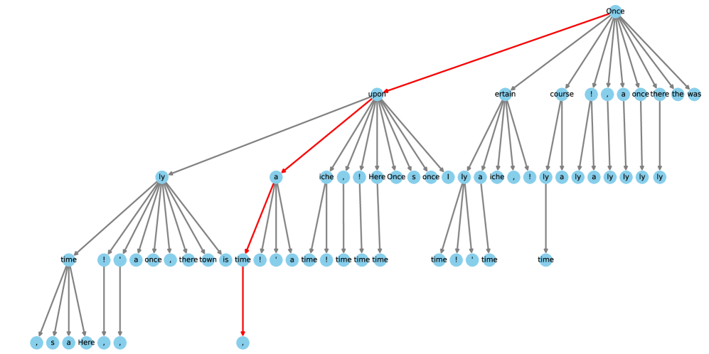
### Visual Description
# Technical Document Extraction: Hierarchical Word Tree Diagram
## 1. Image Overview
This image is a directed graph or "word tree" diagram, likely representing a predictive text model, a suffix tree, or a linguistic probability map. It visualizes the relationships between words and punctuation marks in a hierarchical structure. The diagram uses light blue circular nodes containing text, connected by grey and red directed arrows.
## 2. Component Isolation
### Region A: Root Node (Top Right)
The tree originates from a single root node labeled **"Once"**.
### Region B: Primary Branches (Level 1)
From the root node "Once", there are 10 directed edges leading to the following nodes (ordered roughly left to right):
1. **upon** (connected via a **red** arrow)
2. **ertain**
3. **course**
4. **!**
5. **,**
6. **a**
7. **once**
8. **there**
9. **the**
10. **was**
### Region C: Secondary Branches (Level 2)
The node **"upon"** serves as a secondary hub, branching into several subsequent nodes:
- **a** (connected via a **red** arrow)
- **the**
- **time**
- **an**
- **his**
- **their**
- **this**
- **my**
- **every**
- **that**
### Region D: Tertiary Branches (Level 3)
The node **"a"** (following "upon") branches further into:
- **time** (connected via a **red** arrow)
- **midnight**
- **summer**
- **bright**
- **dark**
- **cold**
- **long**
- **certain**
- **dreary**
- **stormy**
## 3. Visual Encoding and Symbology
- **Nodes**: Light blue circles with black sans-serif text.
- **Edges (Arrows)**:
- **Grey Arrows**: Represent standard transitions or lower-probability paths.
- **Red Arrows**: Highlight a specific path or the highest-probability sequence: **"Once" → "upon" → "a" → "time"**.
- **Directionality**: The graph flows generally from right to left and top to bottom, indicating a temporal or sequential progression of text.
</details>
Figure 6: Visualization of a sparse tree setting for Medusa -2 Vicuna-7B. The tree has 64 nodes representing candidate tokens and a depth of 4 which indicates 4 Medusa heads involved in calculation. Each node indicates a token from a top-k prediction of a Medusa head, and the edges show the connections between them. The red lines highlight the path that correctly predicts the future tokens.
Appendix D Results of Speculative Decoding
In this study, speculative decoding was applied to Vicuna models (Chiang et al., 2023) with varying sizes, specifically 7B, 13B, and 33B. The preliminary framework utilized open-source models such as Llama-68M and 160M (Miao et al., 2023), alongside Tiny-Llama (Zhang et al., 2024) and Tiny-Vicuna (Pan, 2023), fine-tuned from Tiny-Llama with the Vicuna-style instructional tuning strategy. Due to the proprietary nature of speculative decoding methods (Chen et al., 2023; Leviathan et al., 2022), open-source alternatives https://github.com/feifeibear/LLMSpeculativeSampling were deployed for evaluation. Additionally, we utilize torch.compile() to accelerate the inference speed of draft models.
Our results shown in Fig. 7, reveal that the optimal settings of the draft model vary with the Vicuna model sizes. Specifically, the Llama-68M, with a setting of the draft token number $\gamma=4$ , yielded the best performance for Vicuna-7B, while the same draft model with $\gamma=3$ was most effective for Vicuna-13B. For the larger Vicuna-33B, the Tiny-Vicuna (Vicuna-1B), with $\gamma=3$ , provided the greatest acceleration. These results suggest that the choice and setting of the drafting model should be tailored to the size of the LLMs, presenting an area for further exploration in the field.
<details>
<summary>x8.png Details</summary>
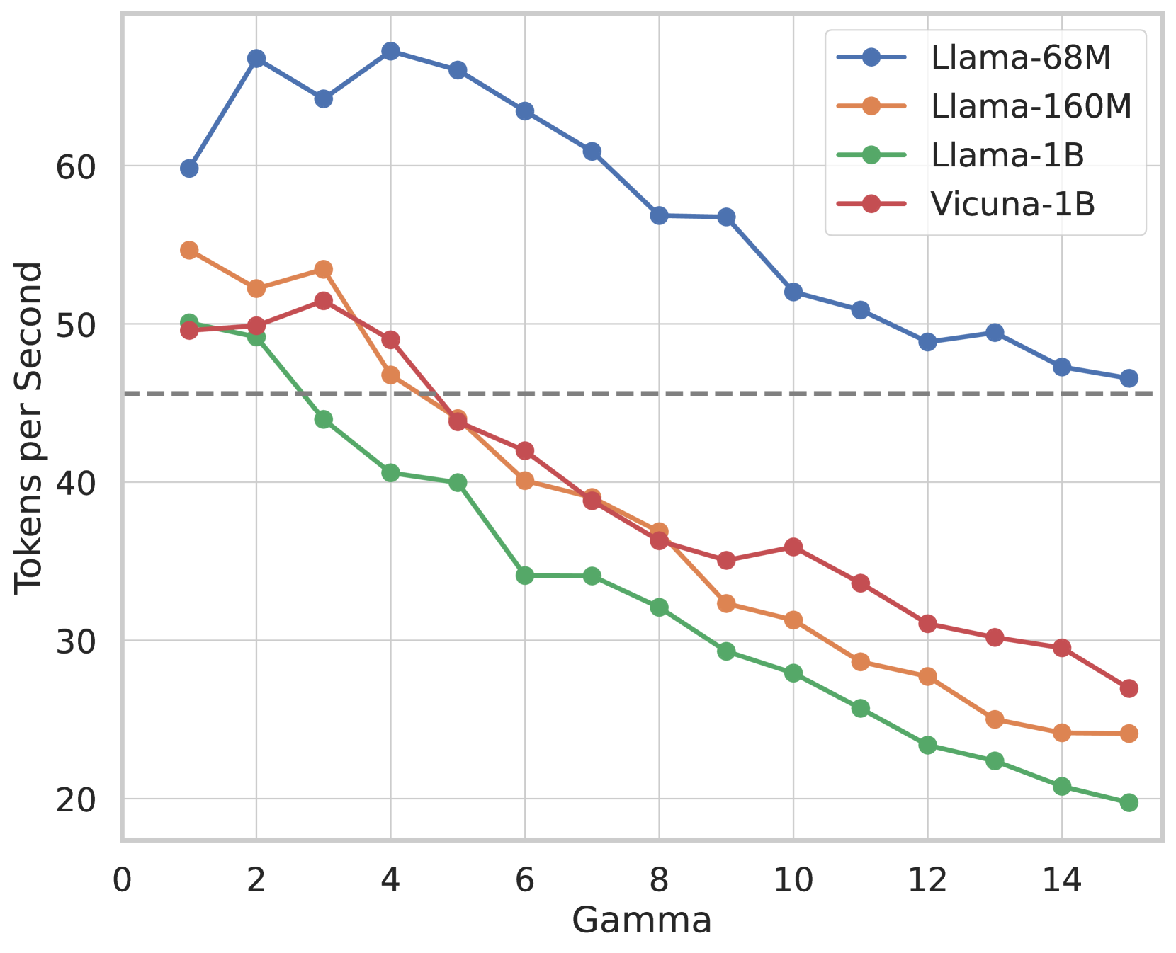
### Visual Description
# Technical Data Extraction: Performance Comparison of Llama and Vicuna Models
## 1. Image Overview
This image is a line graph illustrating the relationship between a parameter labeled **"Gamma"** (x-axis) and the processing speed measured in **"Tokens per Second"** (y-axis). It compares four distinct Large Language Model (LLM) configurations.
## 2. Component Isolation
### Header/Legend
* **Location:** Top-right quadrant [x: ~0.7, y: ~0.1].
* **Legend Items:**
* **Blue line with circular markers:** `Llama-68M`
* **Orange line with circular markers:** `Llama-160M`
* **Green line with circular markers:** `Llama-1B`
* **Red line with circular markers:** `Vicuna-1B`
### Main Chart Area
* **X-Axis Label:** `Gamma`
* **X-Axis Scale:** Linear, ranging from `0` to `15` with major tick marks every 2 units (0, 2, 4, 6, 8, 10, 12, 14).
* **Y-Axis Label:** `Tokens per Second`
* **Y-Axis Scale:** Linear, ranging from `20` to `70` (implied higher) with major tick marks every 10 units (20, 30, 40, 50, 60).
* **Reference Line:** A horizontal dashed grey line is positioned at approximately `y = 45.5`.
## 3. Trend Verification and Data Extraction
All four data series exhibit a general **downward trend** as Gamma increases, though the rate of decay and starting performance vary significantly by model size.
### Data Table (Approximate Values)
| Gamma | Llama-68M (Blue) | Llama-160M (Orange) | Vicuna-1B (Red) | Llama-1B (Green) |
| :--- | :--- | :--- | :--- | :--- |
| 1 | ~60 | ~55 | ~50 | ~50 |
| 2 | ~67 | - | - | ~49 |
| 3 | - | ~54 | ~52 | - |
| 4 | ~68 (Peak) | - | - | ~41 |
| 6 | - | ~40 | - | ~34 |
| 7 | - | ~39 | ~39 | - |
| 8 | ~57 | - | - | - |
| 10 | - | ~31 | - | - |
| 11 | - | - | ~34 | - |
| 15 | ~47 | ~24 | ~27 | ~20 |
### Series Analysis
* **Llama-68M (Blue):** Highest overall performance. It peaks early at Gamma=4 before a steady decline, maintaining a significant lead over all other models.
* **Llama-160M (Orange):** Starts as the second-fastest model. It shows a consistent decline, crossing below the 40 tokens/sec threshold around Gamma=7.
* **Vicuna-1B (Red):** Starts similarly to Llama-1B but maintains higher performance than the 1B Llama variant across all Gamma values > 2. It follows a smoother decay curve than the Llama-160M.
* **Llama-1B (Green):** Lowest overall performance. It experiences a sharp drop between Gamma 2 and Gamma 6, eventually plateauing slightly but remaining the slowest model.
## 4. Summary of Findings
* **Model Size Correlation:** There is a clear inverse correlation between model parameter count and tokens per second. The smallest model (68M) is roughly 2-3x faster than the largest models (1B) at high Gamma values.
* **Gamma Impact:** Increasing the Gamma value negatively impacts throughput across all tested models.
* **Architecture Comparison:** At the 1B parameter scale, the `Vicuna-1B` consistently outperforms the `Llama-1B` in terms of tokens per second for nearly all Gamma values shown.
* **Baseline:** The dashed line at ~45.5 tokens/sec serves as a performance benchmark; only the Llama-68M remains consistently above this line for the entire Gamma range.
</details>
(a) Vicuna-7B
<details>
<summary>x9.png Details</summary>
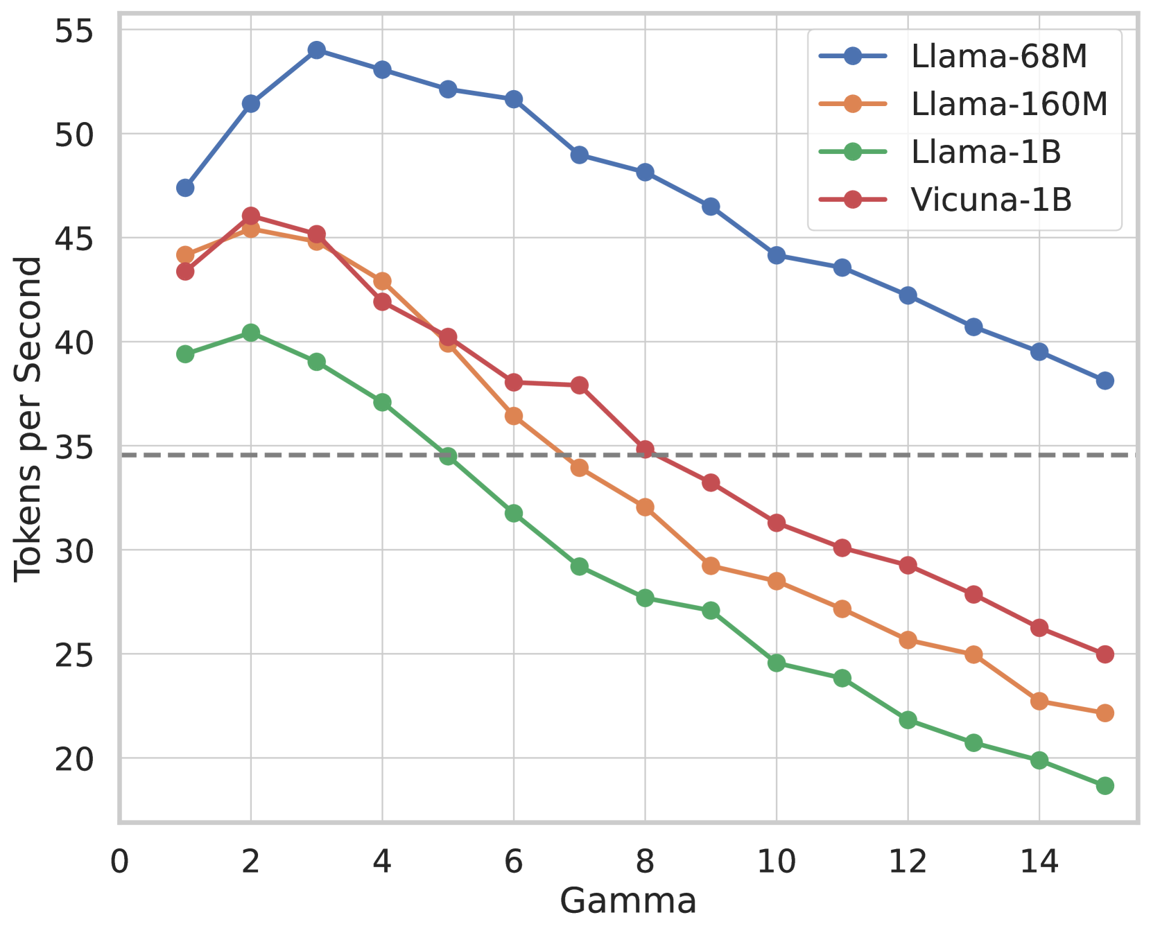
### Visual Description
# Technical Document Extraction: Performance Analysis Chart
## 1. Component Isolation
* **Header:** None present.
* **Main Chart Area:** A line graph with markers plotted on a white grid background. It features four distinct data series and a horizontal reference line.
* **Legend:** Located in the top-right quadrant of the chart area.
* **Axes:**
* **Y-Axis (Vertical):** Labeled "Tokens per Second". Scale ranges from 20 to 55 with increments of 5.
* **X-Axis (Horizontal):** Labeled "Gamma". Scale ranges from 0 to 15 with increments of 2.
---
## 2. Legend and Data Series Identification
The legend is positioned at approximately `[x=0.85, y=0.15]` relative to the top-right corner.
| Series Label | Line Color | Marker Style | Visual Trend Description |
| :--- | :--- | :--- | :--- |
| **Llama-68M** | Blue | Solid circle | Increases sharply to a peak at Gamma=3, then follows a steady, gradual decline. Remains the highest performing series throughout. |
| **Llama-160M** | Orange | Solid circle | Increases to a peak at Gamma=2, then declines steadily. It generally sits between the Vicuna-1B and Llama-1B lines after Gamma=5. |
| **Llama-1B** | Green | Solid circle | Increases to a peak at Gamma=2, then declines steadily. This is the lowest performing series across all Gamma values. |
| **Vicuna-1B** | Red | Solid circle | Increases to a peak at Gamma=2, then declines. It maintains a higher throughput than Llama-160M and Llama-1B for Gamma values > 5. |
---
## 3. Data Extraction
### Reference Line
* **Type:** Horizontal dashed grey line.
* **Value:** Approximately **34.5 Tokens per Second**.
### Numerical Data Points (Estimated from Grid)
Values are extracted by cross-referencing marker positions against the Y-axis (Tokens per Second) and X-axis (Gamma).
| Gamma | Llama-68M (Blue) | Llama-160M (Orange) | Llama-1B (Green) | Vicuna-1B (Red) |
| :--- | :--- | :--- | :--- | :--- |
| **1** | 47.5 | 44.2 | 39.4 | 43.4 |
| **2** | 51.5 | 45.4 | 40.5 | 46.1 |
| **3** | 54.0 | 44.9 | 39.1 | 45.2 |
| **4** | 53.1 | 42.9 | 37.1 | 41.9 |
| **5** | 52.1 | 39.9 | 34.5 | 40.2 |
| **6** | 51.7 | 36.4 | 31.8 | 38.1 |
| **7** | 49.0 | 34.0 | 29.2 | 37.9 |
| **8** | 48.2 | 32.1 | 27.7 | 34.9 |
| **9** | 46.5 | 29.3 | 27.1 | 33.3 |
| **10** | 44.2 | 28.5 | 24.6 | 31.4 |
| **11** | 43.6 | 27.2 | 23.8 | 30.1 |
| **12** | 42.3 | 25.7 | 21.8 | 29.3 |
| **13** | 40.7 | 25.0 | 20.7 | 27.9 |
| **14** | 39.5 | 22.7 | 19.9 | 26.3 |
| **15** | 38.1 | 22.2 | 18.7 | 25.0 |
---
## 4. Key Trends and Observations
1. **Optimal Gamma:** All models exhibit an initial performance increase, peaking at low Gamma values. Llama-68M peaks at **Gamma=3**, while the other three models (Llama-160M, Llama-1B, Vicuna-1B) peak earlier at **Gamma=2**.
2. **Inverse Correlation:** Beyond the peak (Gamma > 3), there is a clear inverse correlation between the Gamma value and Tokens per Second; as Gamma increases, throughput decreases for all models.
3. **Model Size vs. Speed:** There is a general trend where smaller models (Llama-68M) perform significantly faster than larger models (Llama-1B). However, Vicuna-1B (Red) outperforms the smaller Llama-160M (Orange) for Gamma values of 7 and above.
4. **Performance Threshold:** The Llama-68M model remains above the ~34.5 tokens/sec reference line for the entire tested range. In contrast, Llama-1B falls below this threshold after Gamma=5.
</details>
(b) Vicuna-13B
<details>
<summary>x10.png Details</summary>
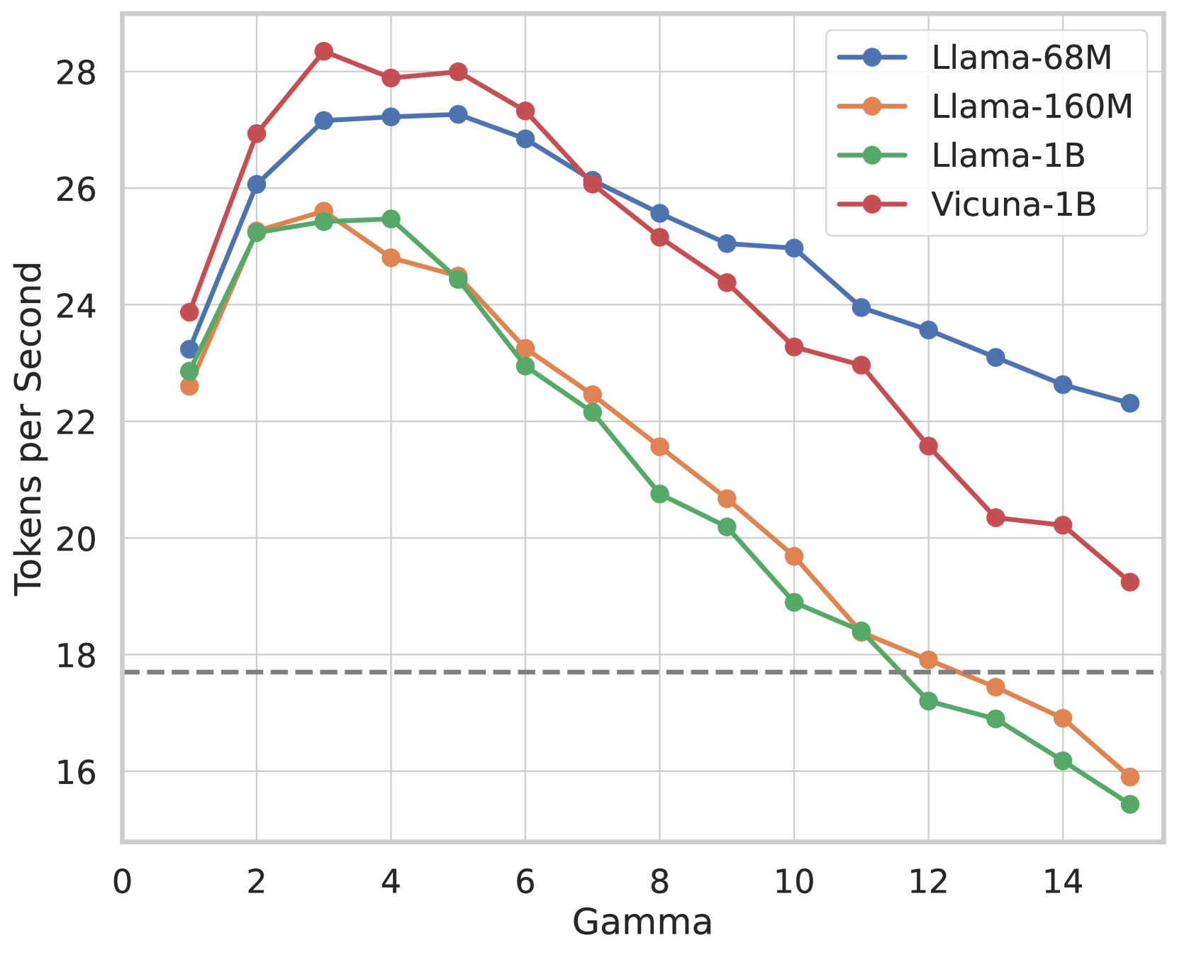
### Visual Description
# Technical Document Extraction: Performance Analysis of LLM Models
## 1. Image Overview
This image is a line graph illustrating the relationship between a parameter labeled **Gamma** and the processing speed measured in **Tokens per Second**. The chart compares four different Large Language Model (LLM) configurations.
## 2. Component Isolation
### Header / Metadata
* **Language:** English
* **Legend Location:** Top-right corner [approx. x=0.7, y=0.1 relative to chart area].
* **Legend Items:**
* **Blue line with circles:** Llama-68M
* **Orange line with circles:** Llama-160M
* **Green line with circles:** Llama-1B
* **Red line with circles:** Vicuna-1B
### Main Chart Area
* **X-Axis Label:** Gamma
* **X-Axis Scale:** Linear, ranging from 0 to 15 (markers every 2 units: 0, 2, 4, 6, 8, 10, 12, 14).
* **Y-Axis Label:** Tokens per Second
* **Y-Axis Scale:** Linear, ranging from 16 to 28 (markers every 2 units: 16, 18, 20, 22, 24, 26, 28).
* **Baseline:** A horizontal dashed grey line is positioned at approximately **y = 17.7**, representing a performance threshold or baseline.
---
## 3. Trend Verification and Data Extraction
### General Trend Analysis
All four models follow a similar non-linear trajectory:
1. **Initial Increase:** Performance rises sharply as Gamma increases from 1 to approximately 3 or 4.
2. **Peak Performance:** Each model reaches a maximum throughput between Gamma 3 and 5.
3. **Steady Decline:** Beyond Gamma 5, all models show a consistent decrease in Tokens per Second as Gamma increases.
### Data Series Details
| Gamma | Llama-68M (Blue) | Llama-160M (Orange) | Llama-1B (Green) | Vicuna-1B (Red) |
| :--- | :--- | :--- | :--- | :--- |
| **1** | ~23.2 | ~22.6 | ~22.9 | ~23.9 |
| **2** | ~26.1 | ~25.3 | ~25.3 | ~27.0 |
| **3** | ~27.2 | ~25.6 | ~25.4 | **~28.3 (Peak)** |
| **4** | ~27.2 | ~24.8 | ~25.5 | ~27.9 |
| **5** | **~27.3 (Peak)** | ~24.5 | ~24.4 | ~28.0 |
| **6** | ~26.9 | ~23.3 | ~23.0 | ~27.3 |
| **7** | ~26.1 | ~22.5 | ~22.2 | ~26.1 |
| **8** | ~25.6 | ~21.6 | ~20.8 | ~25.2 |
| **9** | ~25.1 | ~20.7 | ~20.2 | ~24.4 |
| **10** | ~25.0 | ~19.7 | ~18.9 | ~23.3 |
| **11** | ~24.0 | ~18.4 | ~18.4 | ~23.0 |
| **12** | ~23.6 | ~17.9 | ~17.2 | ~21.6 |
| **13** | ~23.1 | ~17.5 | ~16.9 | ~20.4 |
| **14** | ~22.6 | ~16.9 | ~16.2 | ~20.2 |
| **15** | ~22.3 | ~15.9 | ~15.5 | ~19.3 |
---
## 4. Key Observations
* **Highest Throughput:** The **Vicuna-1B (Red)** model achieves the highest overall performance, peaking at over 28 tokens/sec at Gamma=3.
* **Efficiency Retention:** The **Llama-68M (Blue)** model is the most resilient to increasing Gamma values. While it doesn't reach the absolute peak of Vicuna-1B, its performance degrades much more slowly, remaining above 22 tokens/sec even at Gamma=15.
* **Model Size Impact:** Interestingly, the smaller **Llama-68M** outperforms the larger **Llama-160M** and **Llama-1B** across almost the entire range of Gamma values shown.
* **Baseline Comparison:**
* **Llama-68M** and **Vicuna-1B** remain above the dashed baseline (17.7) for the entire tested range.
* **Llama-160M** falls below the baseline at approximately Gamma=13.
* **Llama-1B** falls below the baseline at approximately Gamma=11.5.
</details>
(c) Vicuna-33B
Figure 7: Inference speed of various models using speculative decoding on MT-Bench. Baseline model speeds are presented by grey dotted lines for comparison. $\gamma$ denotes the draft token number.
Appendix E Additional Results for All Models
We show speedup on various models in Fig. 8.
<details>
<summary>x11.png Details</summary>
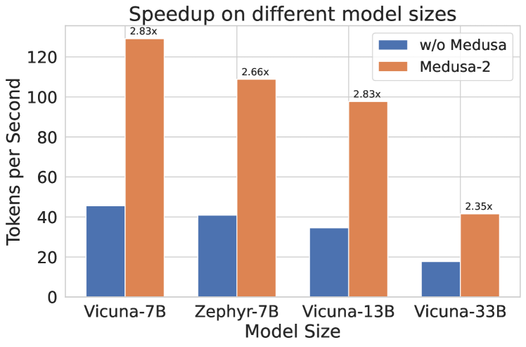
### Visual Description
# Technical Document Extraction: Speedup on Different Model Sizes
## 1. Document Overview
This image is a grouped bar chart illustrating the performance improvements (speedup) achieved by using "Medusa-2" compared to a baseline without it ("w/o Medusa") across four different Large Language Model (LLM) configurations.
## 2. Component Isolation
### Header
* **Title:** Speedup on different model sizes
### Main Chart Area
* **Y-Axis Label:** Tokens per Second
* **Y-Axis Markers:** 0, 20, 40, 60, 80, 100, 120
* **X-Axis Label:** Model Size
* **X-Axis Categories:** Vicuna-7B, Zephyr-7B, Vicuna-13B, Vicuna-33B
* **Legend:**
* **Blue Bar:** w/o Medusa
* **Orange Bar:** Medusa-2
## 3. Data Extraction and Trend Verification
### Trend Analysis
Across all four model sizes, the baseline performance ("w/o Medusa") decreases as the model size increases (from 7B to 33B). Conversely, the "Medusa-2" configuration consistently and significantly outperforms the baseline in every category. The relative speedup (annotated above the orange bars) ranges from 2.35x to 2.83x.
### Data Table (Reconstructed)
| Model Size | w/o Medusa (Tokens/sec) | Medusa-2 (Tokens/sec) | Speedup Factor (Annotated) |
| :--- | :---: | :---: | :---: |
| **Vicuna-7B** | ~45 | ~128 | 2.83x |
| **Zephyr-7B** | ~41 | ~109 | 2.66x |
| **Vicuna-13B** | ~35 | ~98 | 2.83x |
| **Vicuna-33B** | ~18 | ~42 | 2.35x |
## 4. Detailed Observations
* **Baseline Performance:** The baseline (blue) shows a clear downward trend as model complexity increases. Vicuna-7B starts at approximately 45 tokens/sec, while the much larger Vicuna-33B drops to under 20 tokens/sec.
* **Medusa-2 Performance:** The Medusa-2 (orange) enhancement maintains a much higher throughput. Even for the largest model (Vicuna-33B), Medusa-2 achieves a throughput (~42 tokens/sec) nearly equal to the baseline performance of the smallest model (Vicuna-7B at ~45 tokens/sec).
* **Peak Speedup:** The highest relative performance gains are seen in the Vicuna-7B and Vicuna-13B models, both achieving a **2.83x** increase in tokens per second.
* **Visual Style:** The chart uses a clean, white-grid background with sans-serif typography. The bars are grouped by model size to facilitate direct comparison between the two states (with and without Medusa).
</details>
Figure 8: Speedup of various models with Medusa -2. Medusa -2 shows significant speed improvement over all the models, while models trained with self-distillation (Zephyr-7B, Vicuna-13/33B) have weaker speedup due to the trade-off between preserving quality and boosting speed.
Appendix F Additional Results on AlpacalEval Dataset
We conduct further experiments on the AlpacaEval (Li et al., 2023) dataset. Medusa -2 achieves consistent speedup similar to the results on MT-Bench.
| Vicuna-7b Vicuna-13b Vicuna-33b | 37.07 29.01 17.87 | 106.76 91.54 40.43 | 3.23 3.28 2.85 | 2.88 3.16 2.26 |
| --- | --- | --- | --- | --- |
| Zephyr-7b | 34.21 | 99.50 | 3.08 | 2.91 |
Table 4: Speedup results on AlpacaEval (Li et al., 2023) dataset.
Appendix G Exploration and Modeling of Hardware Constraints and Medusa
We explore the hardware constraints, specifically memory-bandwidth bound, and their impact on Medusa -style parallel decoding by incorporating a simplified Llama-series model. First, we identify that the operators involving matrix multiplications, such as linear layers and attention matrix multiplications, are the primary sources of overhead. We profile the performance of FLOP/s vs. Operational Intensity which is the ratio of FLOP/s to bandwidth (bytes/s), across various GPUs, including the A100-80GB-PCIe, A40, and A6000. Next, we examine the changes in FLOP/s vs. Operational Intensity when using Medusa for different operators. Finally, we apply a straightforward analytical model to calculate acceleration rates and combine it with hardware benchmarks. This provides insights into the effects under different model sizes, sequence lengths, and batch sizes.
G.1 Roofline Model of Operators
We present an analysis of the roofline model for various operators in large language models (LLMs), specifically focusing on Llama-7B, Llama-13B, and Llama-33B (Touvron et al., 2023). These models were benchmarked on different GPUs, including the A100-80GB-PCIe, A40, and A6000. We looked into the three categories of matrix multiplication operators since they represent the primary sources of computational overhead in these models. Our study follows the report (Chen, 2023) which investigates the effectiveness of batch size but ours focuses more on decoding and parallel decoding.
Table 5 details the computation and space complexity for each operator during the prefill, decoding, and Medusa decoding phases. The operators include the linear layers for query, key, and value matrices ( $XW_{Q}$ , $XW_{K}$ , $XW_{V}$ ), the attention matrix multiplications ( $QK^{T}$ , $PV$ ), and the up/gate/down linear layers ( $XW_{u}$ , $XW_{g}$ , $XW_{d}$ ). $b$ stands for the batch size, $s$ stands for the sequence length, $h$ stands for the hidden dimension, $i$ stands for the intermediate dimension, $n$ stands for the number of attention heads, $d$ stands for the head dimension and $q$ stands for the candidate length for Medusa. For more details of these operators please refer to the articles (Touvron et al., 2023; Chen, 2023).
Table 5: Computational and space complexity of the main operators in different phases. The table is based on Table 2 in the report (Chen, 2023).
| Operator Prefill $XW_{Q}$ , $XW_{K}$ , $XW_{V}$ | Input Shape $(b,s,h)$ | Output Shape $(b,s,h)$ | Comp. Complexity $O(bsh^{2})$ | Space Complexity $O(2bsh+h^{2})$ |
| --- | --- | --- | --- | --- |
| $QK^{T}$ | $(b,n,s,d),(b,n,s,d)$ | $(b,n,s,s)$ | $O(bs^{2}nd)$ | $O(2bsnd+bs^{2}n)$ |
| $PV$ | $(b,n,s,s),(b,n,s,d)$ | $(b,n,s,d)$ | | |
| $XW_{u}$ , $XW_{g}$ | $(b,s,h)$ | $(b,s,i)$ | $O(bshi)$ | $O(bs(h+i)+hi)$ |
| $XW_{d}$ | $(b,s,i)$ | $(b,s,h)$ | | |
| Decoding | | | | |
| $XW_{Q}$ , $XW_{K}$ , $XW_{V}$ | $(b,1,h)$ | $(b,1,h)$ | $O(bh^{2})$ | $O(2bh+h^{2})$ |
| $QK^{T}$ | $(b,n,1,d),(b,n,s,d)$ | $(b,n,s,1)$ | $O(bsnd)$ | $O(bsn+bsnd+bnd)$ |
| $PV$ | $(b,n,s,1),(b,n,1,d)$ | $(b,n,1,d)$ | | |
| $XW_{u}$ , $XW_{g}$ | $(b,1,h)$ | $(b,1,i)$ | $O(bhi)$ | $O(b(h+i)+hi)$ |
| $XW_{d}$ | $(b,1,i)$ | $(b,1,h)$ | | |
| Parallel decoding | | | | |
| $XW_{Q}$ , $XW_{K}$ , $XW_{V}$ | $(b,q,h)$ | $(b,q,h)$ | $O(bqh^{2})$ | $O(2bqh+h^{2})$ |
| $QK^{T}$ | $(b,n,q,d),(b,n,s,d)$ | $(b,n,s,q)$ | $O(bsqnd)$ | $O(bsqn+b(s+q)nd)$ |
| $PV$ | $(b,n,s,q),(b,n,q,d)$ | $(b,n,q,d)$ | | |
| $XW_{u}$ , $XW_{g}$ | $(b,q,h)$ | $(b,q,i)$ | $O(bqhi)$ | $O(bq(h+i)+hi)$ |
| $XW_{d}$ | $(b,q,i)$ | $(b,q,h)$ | | |
Figures 9 - 17 show the benchmark of three categories of operators on different models (7/13/33B) under various settings. To evaluate each operator’s performance and throughput, we chose the combination of settings including batch sizes from 1 to 64 in powers of 2 and sequence lengths from 128 to 8192 in powers of 2 (49 settings for each operator). From all the figures, we observe that the datapoints of each operator in the prefill and decoding stages cluster at very similar positions across all GPUs and for various model sizes.
During the prefill phase, increasing the batch size changes the FLOP/s of the attention matrix multiplications (see ‘qk/pv init‘) but does not affect the Operational Intensity (refer to the vertical dashed arrow in Fig. 9). In contrast, increasing the sequence length impacts both FLOP/s and Operational Intensity in the prefill phase (refer to the diagonal dashed arrow in Fig. 9). During the decoding phase, the attention matrix multiplications are significantly limited by memory bandwidth. Despite an increase in FLOP/s with changes in batch size and sequence length, the Operational Intensity remains nearly unchanged (see ‘qk/pv ar‘). This indicates suboptimal resource utilization in the self-attention mechanism.
The linear layers in the prefill phase are mostly compute-bound (see ‘qkv mlp init‘ and ‘up/gate/down init‘). During the decoding phase, the datapoints of the linear layer form a line with the same slope as the GPU’s memory bandwidth (see ‘qkv mlp ar‘ and ‘up/gate/down ar‘). This indicates the linear layers in the decoding stage are also bounded by memory bandwidth. Increasing the batch size improves the achieved FLOP/s and Operational Intensity under memory bandwidth constraints through better parallelism. Note that linear layers only process the new token and are independent of sequence length (See ‘Decoding‘ section in Table 5).
<details>
<summary>x12.png Details</summary>
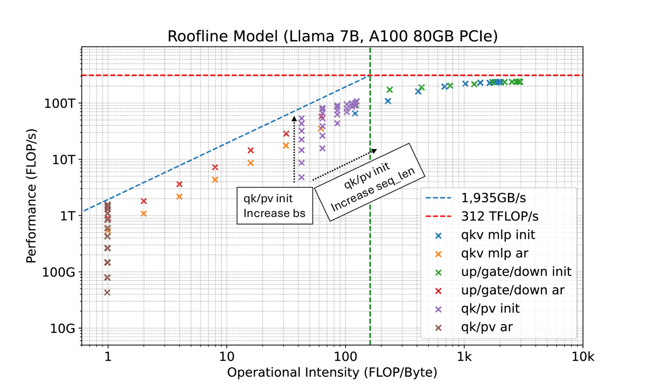
### Visual Description
# Technical Document Extraction: Roofline Model (Llama 7B, A100 80GB PCIe)
## 1. Header Information
* **Title:** Roofline Model (Llama 7B, A100 80GB PCIe)
* **Subject:** Performance analysis of a Llama 7B model running on an NVIDIA A100 80GB PCIe GPU.
## 2. Chart Specifications
The image is a **Roofline Chart**, a log-log plot used to visualize the performance of algorithms against hardware limits.
### Axis Definitions
* **Y-Axis (Vertical):** Performance (FLOP/s)
* **Scale:** Logarithmic, ranging from 10G to 100T+.
* **Major Markers:** 10G, 100G, 1T, 10T, 100T.
* **X-Axis (Horizontal):** Operational Intensity (FLOP/Byte)
* **Scale:** Logarithmic, ranging from 1 to 10k.
* **Major Markers:** 1, 10, 100, 1k, 10k.
### Hardware Limits (The "Roofline")
The chart features two primary hardware constraint lines that form the "roof":
1. **Memory Bandwidth Limit (Sloped Blue Dashed Line):**
* **Label:** 1,935GB/s
* **Trend:** Slopes upward from left to right. This represents the memory-bound region where performance is limited by how fast data can be moved from memory.
2. **Peak Compute Limit (Horizontal Red Dashed Line):**
* **Label:** 312 TFLOP/s
* **Trend:** Horizontal. This represents the compute-bound region where the GPU's processing power is the bottleneck.
3. **Ridge Point (Vertical Green Dashed Line):**
* **Location:** Approximately 161 FLOP/Byte (where the bandwidth and compute lines intersect).
## 3. Legend and Data Series
The legend is located in the bottom-right quadrant of the chart.
| Symbol | Color | Label | Description/Trend |
| :--- | :--- | :--- | :--- |
| `--` | Blue | 1,935GB/s | Memory bandwidth ceiling. |
| `--` | Red | 312 TFLOP/s | Peak theoretical compute performance. |
| `x` | Blue | qkv mlp init | Initialization phase for QKV and MLP layers. Points cluster between 100 and 1k FLOP/Byte, approaching the compute ceiling. |
| `x` | Orange | qkv mlp ar | Autoregressive (AR) phase for QKV and MLP. Points are at low operational intensity (~1 to 10 FLOP/Byte), following the bandwidth slope. |
| `x` | Green | up/gate/down init | Initialization for Feed-Forward Network (FFN) layers. High intensity (1k - 3k FLOP/Byte), sitting directly on the 312 TFLOP/s ceiling. |
| `x` | Red | up/gate/down ar | AR phase for FFN layers. Low intensity (~1 to 40 FLOP/Byte), following the bandwidth slope. |
| `x` | Purple | qk/pv init | Initialization for Attention (QK/PV) operations. Clustered between 40 and 150 FLOP/Byte. |
| `x` | Brown | qk/pv ar | AR phase for Attention operations. Very low intensity, clustered at the 1 FLOP/Byte mark. |
## 4. Annotated Trends and Logic Checks
The chart contains specific callouts explaining how changing parameters affects performance:
### Component: qk/pv init (Purple 'x' markers)
* **Vertical Trend (Increase bs):** A vertical dotted arrow points upward through the purple markers.
* **Text Box:** `qk/pv init Increase bs`
* **Interpretation:** Increasing the **batch size (bs)** increases the Performance (FLOP/s) without significantly changing the Operational Intensity.
* **Diagonal Trend (Increase seq_len):** A diagonal dotted arrow points upward and to the right through the purple markers.
* **Text Box:** `qk/pv init Increase seq_len`
* **Interpretation:** Increasing the **sequence length (seq_len)** increases both the Operational Intensity and the Performance, moving the kernels closer to the compute-bound "roof."
## 5. Summary of Observations
* **Memory Bound:** Most "ar" (autoregressive/decoding) kernels (Orange, Red, Brown) are located on the sloped part of the graph, indicating they are limited by the 1,935 GB/s memory bandwidth.
* **Compute Bound:** Most "init" (initialization/prefill) kernels (Green, Blue, Purple) are located near or on the horizontal red line, indicating they are utilizing the full 312 TFLOP/s compute capacity of the A100.
* **Efficiency:** The `up/gate/down init` (Green) kernels are the most efficient, reaching the theoretical peak of the hardware. The `qk/pv ar` (Brown) kernels are the least efficient, limited by extremely low operational intensity at the far left of the chart.
</details>
Figure 9: The figure shows the relationship between FLOP/s and Operational Intensity for all benchmarked datapoints of Llama-7B operators on A100-80GB-PCIe. The dashed lines represent the HBM bandwidth limit (1,935GB/s) and the peak performance limit (312 TFLOP/s) (NVIDIA, ). ‘ qkv mlp ’ stands for the linear layers projecting hidden features to query/key/value features. ‘ up/gate/down ’ stands for the linear layers following the attention block. ‘ qk/pv ’ stands for the two steps of attention matrix multiplications. ‘ ar ’ stands for the decoding (autoregressive) and ‘ init ’ stands for the prefill phase.
<details>
<summary>x13.png Details</summary>
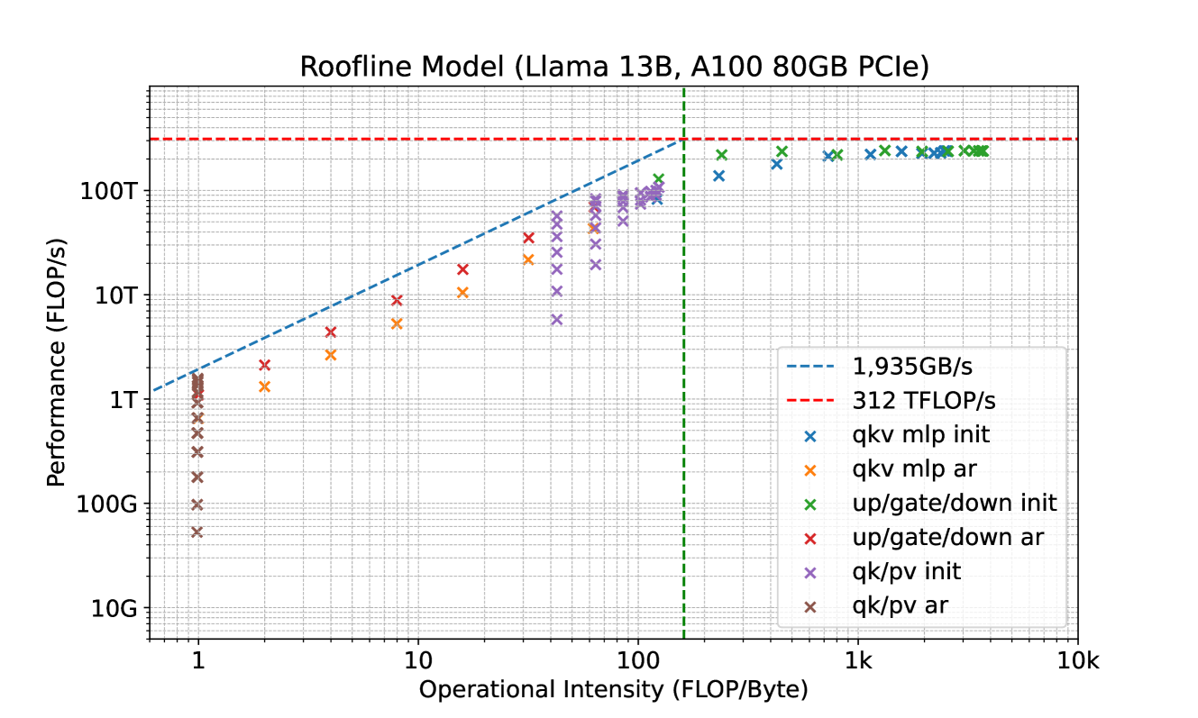
### Visual Description
# Technical Document Extraction: Roofline Model Analysis
## 1. Document Metadata
* **Title:** Roofline Model (Llama 13B, A100 80GB PCIe)
* **Primary Language:** English
* **Chart Type:** Log-Log Roofline Plot (Performance vs. Operational Intensity)
---
## 2. Component Isolation
### A. Header
* **Text:** "Roofline Model (Llama 13B, A100 80GB PCIe)"
* **Context:** This chart evaluates the performance of a Llama 13B large language model running on an NVIDIA A100 80GB PCIe GPU.
### B. Axes and Scale
* **Y-Axis (Vertical):**
* **Label:** Performance (FLOP/s)
* **Scale:** Logarithmic, ranging from 10G to 1000T (10^10 to 10^15).
* **Major Markers:** 10G, 100G, 1T, 10T, 100T.
* **X-Axis (Horizontal):**
* **Label:** Operational Intensity (FLOP/Byte)
* **Scale:** Logarithmic, ranging from 1 to 10k (10^0 to 10^4).
* **Major Markers:** 1, 10, 100, 1k, 10k.
### C. Legend (Spatial Grounding: Bottom Right [x≈0.7, y≈0.2])
The legend defines the theoretical limits and the specific kernel operations measured.
| Legend Item | Color/Style | Description |
| :--- | :--- | :--- |
| **1,935GB/s** | Blue Dashed Line (Sloped) | Memory Bandwidth Limit |
| **312 TFLOP/s** | Red Dashed Line (Horizontal) | Peak Compute Performance Limit |
| **qkv mlp init** | Blue 'x' | Initialization phase for QKV and MLP layers |
| **qkv mlp ar** | Orange 'x' | Autoregressive phase for QKV and MLP layers |
| **up/gate/down init** | Green 'x' | Initialization phase for Up/Gate/Down projection layers |
| **up/gate/down ar** | Red 'x' | Autoregressive phase for Up/Gate/Down projection layers |
| **qk/pv init** | Purple 'x' | Initialization phase for QK/PV attention scores |
| **qk/pv ar** | Brown 'x' | Autoregressive phase for QK/PV attention scores |
---
## 3. Theoretical Limits (The "Roofline")
1. **Memory Bound (Sloped Line):** A blue dashed line representing a bandwidth of **1,935 GB/s**. It slopes upward from left to right, indicating that at low operational intensity, performance is limited by how fast data can be moved from memory.
2. **Compute Bound (Horizontal Line):** A red dashed line representing a peak performance of **312 TFLOP/s**. This is the absolute ceiling for the hardware regardless of operational intensity.
3. **Ridge Point:** A vertical green dashed line marks the intersection of the bandwidth and compute limits, occurring at approximately **161 FLOP/Byte**.
---
## 4. Data Series Analysis and Trends
### Memory-Bound Operations (Low Operational Intensity)
These data points follow the sloped blue line or sit significantly below it at the left side of the chart.
* **qk/pv ar (Brown 'x'):**
* **Trend:** Vertical cluster at Operational Intensity ≈ 1.
* **Performance:** Ranges from ~50G FLOP/s to ~1.5T FLOP/s.
* **Observation:** These are highly memory-bound operations with very low arithmetic intensity.
* **qkv mlp ar (Orange 'x'):**
* **Trend:** Slopes upward following the memory bandwidth limit.
* **Performance:** Starts at ~1.2T FLOP/s (OI ≈ 2) and reaches ~20T FLOP/s (OI ≈ 30).
* **up/gate/down ar (Red 'x'):**
* **Trend:** Slopes upward, slightly higher performance than 'qkv mlp ar' for similar intensities.
* **Performance:** Starts at ~2T FLOP/s (OI ≈ 2) and reaches ~35T FLOP/s (OI ≈ 30).
### Transition and Compute-Bound Operations (High Operational Intensity)
These data points cluster near the horizontal red line at the right side of the chart.
* **qk/pv init (Purple 'x'):**
* **Trend:** Slopes upward from OI ≈ 40 to OI ≈ 120.
* **Performance:** Starts at ~6T FLOP/s and reaches ~120T FLOP/s.
* **qkv mlp init (Blue 'x'):**
* **Trend:** Clustered near the ridge point and beyond (OI ≈ 200 to 3k).
* **Performance:** High performance, ranging from ~150T FLOP/s to ~250T FLOP/s.
* **up/gate/down init (Green 'x'):**
* **Trend:** Clustered at the highest operational intensities (OI ≈ 200 to 4k).
* **Performance:** These are the most efficient operations, consistently hitting the peak compute limit at ~250T - 300T FLOP/s.
---
## 5. Summary of Findings
* **Initialization vs. Autoregressive:** "Init" (Initialization) phases consistently show higher operational intensity and higher performance (closer to the 312 TFLOP/s peak) compared to "ar" (Autoregressive) phases.
* **Bottlenecks:** Autoregressive operations (ar) are severely memory-bound, limited by the 1,935 GB/s bandwidth. Initialization operations (init) are compute-bound or near-compute-bound, utilizing the A100's processing power more effectively.
* **Efficiency:** The "up/gate/down init" operations are the most efficient kernels in this workload, achieving performance closest to the theoretical hardware maximum.
</details>
Figure 10: Llama-13B operators on A100-80GB-PCIe.
<details>
<summary>x14.png Details</summary>

### Visual Description
# Technical Document Extraction: Roofline Model Analysis
## 1. Document Header
* **Title:** Roofline Model (Llama 33B, A100 80GB PCIe)
* **Subject:** Performance analysis of a Llama 33B model running on an NVIDIA A100 80GB PCIe GPU.
## 2. Chart Configuration and Axes
The image is a **Roofline Chart**, a log-log plot used to visualize the performance limits of a computing system based on operational intensity.
* **Y-Axis (Performance):**
* **Label:** Performance (FLOP/s)
* **Scale:** Logarithmic, ranging from 10G to 1000T ($10^{10}$ to $10^{15}$).
* **Major Markers:** 10G, 100G, 1T, 10T, 100T.
* **X-Axis (Operational Intensity):**
* **Label:** Operational Intensity (FLOP/Byte)
* **Scale:** Logarithmic, ranging from approximately 0.6 to 10k ($10^4$).
* **Major Markers:** 1, 10, 1k, 10k.
* **Grid:** Fine dashed grid lines for both axes to assist in precise data point estimation.
## 3. Legend and Theoretical Limits
The legend is located in the bottom-right quadrant of the main chart area.
### Theoretical Bounds (Lines)
| Limit | Label/Value | Trend | Function |
| :--- | :--- | :--- | :--- |
| **Memory Bandwidth Limit** | 1,935 GB/s | Slopes upward (left to right) | Maximum performance when memory-bound. |
| **Compute Peak Limit** | 312 TFLOP/s | Horizontal line | Absolute hardware ceiling for floating-point operations. |
| **Ridge Point** | ~161 FLOP/Byte | Vertical dashed line | Intersection of bandwidth and compute limits. |
### Data Series (Markers)
All data points are represented by "x" markers:
* **Blue (x):** `qkv mlp init`
* **Orange (x):** `qkv mlp ar`
* **Green (x):** `up/gate/down init`
* **Red (x):** `up/gate/down ar`
* **Purple (x):** `qk/pv init`
* **Brown (x):** `qk/pv ar`
## 4. Component Analysis and Data Trends
### Region 1: Memory-Bound (Operational Intensity < 161)
In this region, performance is limited by the speed at which data can be moved from memory. Data points generally follow the slope of the blue dashed line.
* **`qk/pv ar` (Brown):** Lowest operational intensity (~1 FLOP/Byte). Performance ranges vertically from ~60G to ~2T FLOP/s, indicating varying efficiency at the same intensity.
* **`qkv mlp ar` (Orange):** Slopes upward following the bandwidth limit. Operational intensity ranges from ~2 to ~15. Performance ranges from ~2T to ~15T FLOP/s.
* **`up/gate/down ar` (Red):** Similar trend to orange, slightly higher operational intensity (~2 to ~30). Performance reaches up to ~40T FLOP/s.
* **`qk/pv init` (Purple):** High density of points between 40 and 150 FLOP/Byte. Performance scales from ~10T up to ~150T FLOP/s as it approaches the ridge point.
### Region 2: Compute-Bound (Operational Intensity > 161)
In this region, performance is limited by the GPU's processing power. Data points flatten out near the red dashed line.
* **`up/gate/down init` (Green):** Located between 200 and 5,000 FLOP/Byte. These points are clustered very close to the 312 TFLOP/s ceiling, indicating high hardware utilization.
* **`qkv mlp init` (Blue):** Located between 800 and 4,000 FLOP/Byte. These points are also clustered at the 312 TFLOP/s ceiling, representing the most compute-efficient operations in the model.
## 5. Summary of Findings
* **Initialization (init) phases** for `qkv mlp` and `up/gate/down` are highly efficient, reaching the hardware's peak compute capacity (312 TFLOP/s).
* **Autoregressive (ar) phases** and `qk/pv` operations are significantly memory-bound, with operational intensities below 100 FLOP/Byte, preventing them from reaching the peak TFLOP/s of the A100 GPU.
* The **`qk/pv ar`** operations are the most bottlenecked, residing at the far left of the chart with the lowest performance and operational intensity.
</details>
Figure 11: Llama-33B operators on A100-80GB-PCIe.
<details>
<summary>x15.png Details</summary>
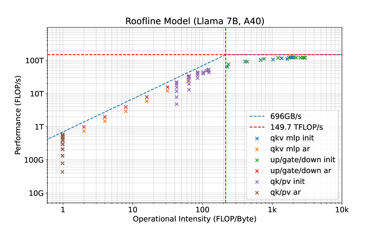
### Visual Description
# Technical Document Extraction: Roofline Model (Llama 7B, A40)
## 1. Document Header
* **Title:** Roofline Model (Llama 7B, A40)
* **Subject:** Performance analysis of a Llama 7B model running on an NVIDIA A40 GPU.
## 2. Chart Specifications
The image is a **Roofline Plot**, a standard visualization for identifying performance bottlenecks in computing (Memory-bound vs. Compute-bound).
### Axis Definitions
* **Y-Axis (Vertical):** Performance (FLOP/s)
* **Scale:** Logarithmic (Base 10).
* **Markers:** 10G, 100G, 1T, 10T, 100T.
* **X-Axis (Horizontal):** Operational Intensity (FLOP/Byte)
* **Scale:** Logarithmic (Base 10).
* **Markers:** 1, 10, 1k (1,000), 10k (10,000).
### Legend and Reference Lines
The legend is located in the bottom-right quadrant of the chart area.
| Label | Color/Style | Description |
| :--- | :--- | :--- |
| **696GB/s** | Blue Dashed Line (Diagonal) | Represents the memory bandwidth limit. Performance increases linearly with operational intensity in this region. |
| **149.7 TFLOP/s** | Red Dashed Line (Horizontal) | Represents the peak theoretical compute performance of the A40 GPU. |
</details>
Figure 12: Llama-7B operators on A40.
<details>
<summary>x16.png Details</summary>
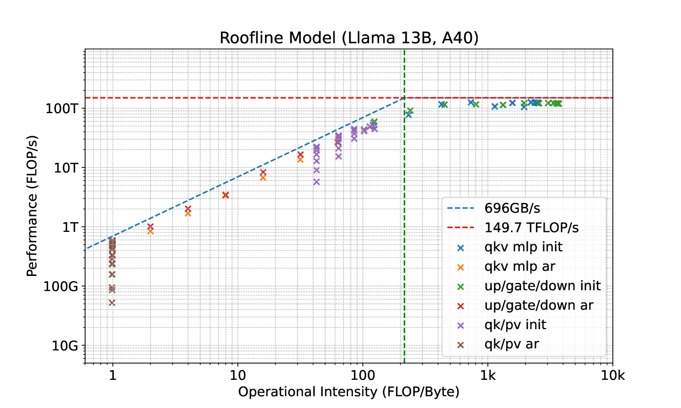
### Visual Description
# Technical Document Extraction: Roofline Model (Llama 13B, A40)
## 1. Document Header
* **Title:** Roofline Model (Llama 13B, A40)
* **Subject:** Performance analysis of the Llama 13B model running on an NVIDIA A40 GPU.
## 2. Chart Specifications
The image is a **Roofline Chart**, a standard visualization used to identify performance bottlenecks in computing workloads.
### Axis Definitions
* **Y-Axis (Vertical):** Performance (FLOP/s)
* **Scale:** Logarithmic (Base 10).
* **Markers:** 10G, 100G, 1T, 10T, 100T.
* **X-Axis (Horizontal):** Operational Intensity (FLOP/Byte)
* **Scale:** Logarithmic (Base 10).
* **Markers:** 1, 10, 100, 1k (1,000), 10k (10,000).
### Legend and Thresholds
The legend is located in the bottom-right quadrant of the chart area.
| Legend Item | Color/Style | Description | Value/Threshold |
| :--- | :--- | :--- | :--- |
| **696GB/s** | Blue Dashed Line | Memory Bandwidth Limit | Slopes upward at 45° (log-log) |
| **149.7 TFLOP/s** | Red Dashed Line | Peak Compute Performance | Horizontal line at ~1.5e14 |
| **Ridge Point** | Green Vertical Dashed | Intersection of Bandwidth and Compute | ~215 FLOP/Byte |
| **qkv mlp init** | Blue 'x' | Initialization phase for QKV/MLP layers | Compute-bound region |
| **qkv mlp ar** | Orange 'x' | Autoregressive phase for QKV/MLP layers | Memory-bound region |
| **up/gate/down init** | Green 'x' | Initialization phase for Up/Gate/Down layers | Compute-bound region |
| **up/gate/down ar** | Red 'x' | Autoregressive phase for Up/Gate/Down layers | Memory-bound region |
| **qk/pv init** | Purple 'x' | Initialization phase for QK/PV layers | Transition region |
| **qk/pv ar** | Brown 'x' | Autoregressive phase for QK/PV layers | Memory-bound region |
---
## 3. Component Analysis and Data Trends
### Region 1: Memory-Bound (Left of the Ridge Point)
* **Visual Trend:** Data points follow the upward slope of the blue dashed line (696GB/s).
* **Observations:**
* **Autoregressive (ar) phases** (Orange, Red, Brown 'x' marks) are clustered here.
* **qk/pv ar (Brown):** Lowest operational intensity (~1 FLOP/Byte), resulting in the lowest performance (between 50G and 1T FLOP/s).
* **up/gate/down ar (Red) & qkv mlp ar (Orange):** Higher intensity than qk/pv ar, ranging from ~2 to ~40 FLOP/Byte. Performance scales linearly with intensity along the bandwidth limit.
### Region 2: Compute-Bound (Right of the Ridge Point)
* **Visual Trend:** Data points flatten out and cluster along the horizontal red dashed line (149.7 TFLOP/s).
* **Observations:**
* **Initialization (init) phases** (Blue, Green 'x' marks) are clustered here.
* **up/gate/down init (Green):** High operational intensity (approx. 400 to 4,000 FLOP/Byte). These points are pinned against the 149.7 TFLOP/s ceiling, indicating maximum hardware utilization.
* **qkv mlp init (Blue):** Similar to the green series, these points sit at the peak performance ceiling with intensities between 1,000 and 3,000 FLOP/Byte.
### Region 3: Transition/Ridge Area
* **Visual Trend:** Points begin to deviate from the bandwidth slope and curve toward the compute ceiling.
* **Observations:**
* **qk/pv init (Purple):** These points bridge the gap, located between 40 and 150 FLOP/Byte. They show performance increasing from 10T to nearly 100T FLOP/s but remain below the absolute peak.
---
## 4. Summary of Findings
1. **Hardware Limits:** The A40 GPU used for Llama 13B has a peak throughput of **149.7 TFLOP/s** and a memory bandwidth of **696 GB/s**.
2. **Bottleneck Identification:**
* **Initialization phases** are **Compute-Bound**. They efficiently utilize the GPU's processing power because they have high operational intensity.
* **Autoregressive phases** (the generation step) are **Memory-Bound**. Their performance is limited by how fast data can be moved from memory, not by the GPU's calculation speed.
3. **Critical Threshold:** The "Ridge Point" occurs at approximately **215 FLOP/Byte**. Any operation with an intensity lower than this will be limited by memory bandwidth.
</details>
Figure 13: Llama-13B operators on A40.
<details>
<summary>x17.png Details</summary>
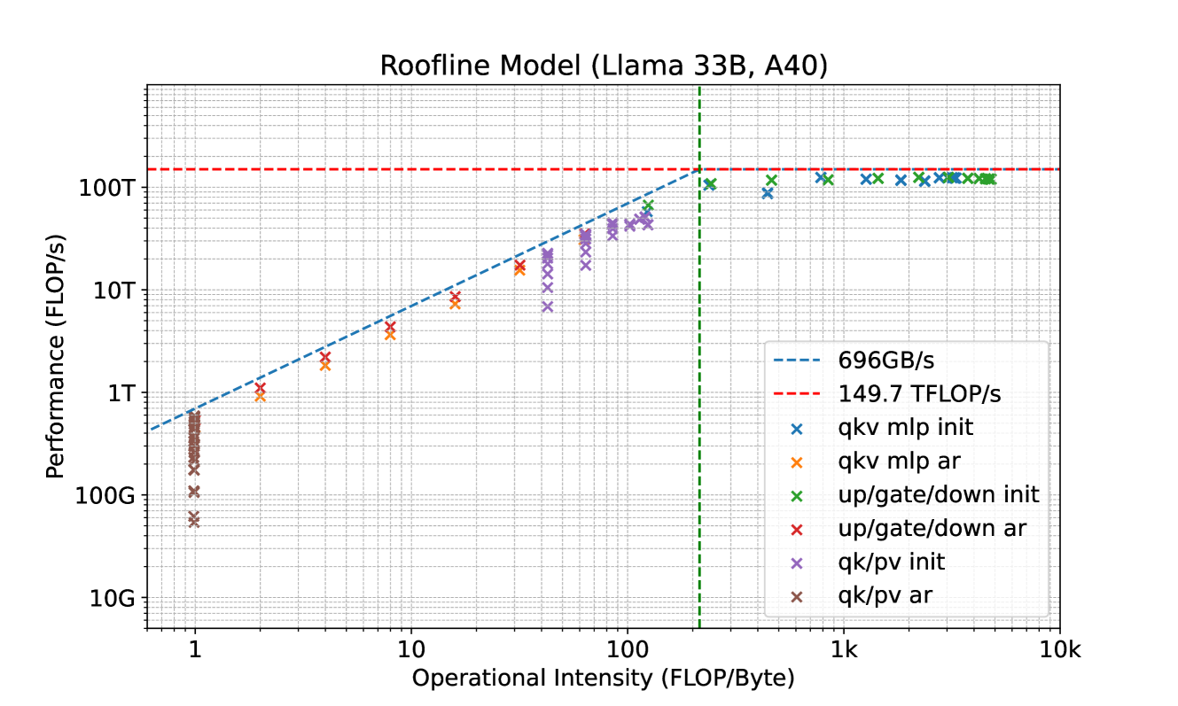
### Visual Description
# Technical Document Extraction: Roofline Model (Llama 33B, A40)
## 1. Header Information
* **Title:** Roofline Model (Llama 33B, A40)
* **Subject:** Performance analysis of the Llama 33B model running on an NVIDIA A40 GPU.
## 2. Chart Specifications
* **Type:** Log-Log Roofline Plot.
* **X-Axis (Horizontal):** Operational Intensity (FLOP/Byte).
* **Scale:** Logarithmic, ranging from approximately 0.6 to 10,000 (10k).
* **Major Markers:** 1, 10, 100, 1k (1,000), 10k (10,000).
* **Y-Axis (Vertical):** Performance (FLOP/s).
* **Scale:** Logarithmic, ranging from 10G to over 100T.
* **Major Markers:** 10G, 100G, 1T, 10T, 100T.
## 3. Legend and Thresholds
The legend is located in the bottom-right quadrant of the chart area.
| Legend Item | Color/Style | Description |
| :--- | :--- | :--- |
| **696GB/s** | Blue Dashed Line (Diagonal) | Memory Bandwidth Limit. Slopes upward from left to right. |
| **149.7 TFLOP/s** | Red Dashed Line (Horizontal) | Peak Compute Performance Limit (Roof). |
| **qkv mlp init** | Blue 'x' | Data points for QKV/MLP initialization. |
| **qkv mlp ar** | Orange 'x' | Data points for QKV/MLP auto-regressive phase. |
| **up/gate/down init** | Green 'x' | Data points for Up/Gate/Down projection initialization. |
| **up/gate/down ar** | Red 'x' | Data points for Up/Gate/Down projection auto-regressive phase. |
| **qk/pv init** | Purple 'x' | Data points for QK/PV initialization. |
| **qk/pv ar** | Brown 'x' | Data points for QK/PV auto-regressive phase. |
*Note: A vertical green dashed line intersects the "elbow" where the bandwidth limit meets the compute limit, occurring at an operational intensity of approximately 215 FLOP/Byte.*
## 4. Component Analysis and Trends
### Memory-Bound Region (Left of the Green Vertical Line)
In this region, performance is limited by memory bandwidth (the diagonal blue line).
* **Trend:** Data points follow the upward slope of the 696GB/s line. As operational intensity increases, performance increases linearly on the log-log scale.
* **Series `qk/pv ar` (Brown):** Clustered at the lowest operational intensity (~1 FLOP/Byte) with performance between 60G and 600G FLOP/s.
* **Series `up/gate/down ar` (Red) & `qkv mlp ar` (Orange):** These follow the diagonal line closely between 2 and 40 FLOP/Byte. Performance ranges from ~1T to ~20T FLOP/s.
* **Series `qk/pv init` (Purple):** Clustered between 40 and 150 FLOP/Byte. These points are slightly below the theoretical bandwidth limit, ranging from ~7T to ~70T FLOP/s.
### Compute-Bound Region (Right of the Green Vertical Line)
In this region, performance is limited by the GPU's peak compute capability (the horizontal red line).
* **Trend:** Data points flatten out and move horizontally, plateauing near the 149.7 TFLOP/s limit.
* **Series `up/gate/down init` (Green):** Located at high operational intensities (approx. 250 to 5,000 FLOP/Byte). These points sit very close to the 149.7 TFLOP/s roof.
* **Series `qkv mlp init` (Blue):** Located at high operational intensities (approx. 400 to 4,000 FLOP/Byte). These points also sit near the peak compute roof, showing high efficiency for initialization tasks.
## 5. Summary of Data Observations
1. **Auto-regressive (ar) tasks** (Brown, Red, Orange) are predominantly **memory-bound**, characterized by low operational intensity and performance that scales with memory bandwidth.
2. **Initialization (init) tasks** (Purple, Green, Blue) have higher operational intensity. While `qk/pv init` is still transitioning, `up/gate/down init` and `qkv mlp init` are clearly **compute-bound**, reaching the hardware's maximum TFLOP/s capacity.
3. The "Ridge Point" or "Elbow" of the machine is at **~215 FLOP/Byte**. Any operation with intensity lower than this cannot reach peak TFLOP/s on an A40.
</details>
Figure 14: Llama-33B operators on A40.
<details>
<summary>x18.png Details</summary>
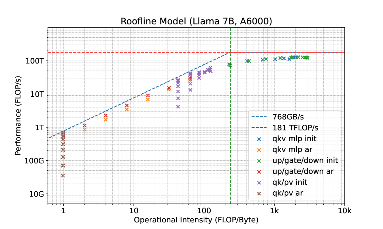
### Visual Description
# Technical Document Extraction: Roofline Model Analysis
## 1. Document Metadata
* **Title:** Roofline Model (Llama 7B, A6000)
* **Primary Language:** English
* **Subject:** Performance analysis of a Llama 7B Large Language Model on an NVIDIA RTX A6000 GPU.
## 2. Chart Structure and Axes
The image is a **Roofline Chart**, a log-log plot used to visualize the performance limits of a computing system based on operational intensity.
### Header Region
* **Title:** Roofline Model (Llama 7B, A6000)
### Main Chart Region
* **Y-Axis (Vertical):** Performance (FLOP/s)
* **Scale:** Logarithmic
* **Markers:** 10G, 100G, 1T, 10T, 100T
* **X-Axis (Horizontal):** Operational Intensity (FLOP/Byte)
* **Scale:** Logarithmic
* **Markers:** 1, 10, 100, 1k (1,000), 10k (10,000)
* **Grid:** Fine-grained logarithmic grid lines are present for both axes.
### Legend Region
**Spatial Placement:** Bottom-right quadrant [approx. x=0.7, y=0.2 relative to chart area].
* **Blue Dashed Line (`--`):** 768GB/s (Memory Bandwidth Limit)
* **Red Dashed Line (`--`):** 181 TFLOP/s (Peak Compute Limit)
* **Blue 'x' Marker:** qkv mlp init
* **Orange 'x' Marker:** qkv mlp ar
* **Green 'x' Marker:** up/gate/down init
* **Red 'x' Marker:** up/gate/down ar
* **Purple 'x' Marker:** qk/pv init
* **Brown 'x' Marker:** qk/pv ar
## 3. Performance Boundaries (The "Roofline")
The chart defines the theoretical maximum performance of the A6000 hardware:
1. **Memory Bound (Sloped Ceiling):** Represented by a blue dashed line with a slope of 1 on the log-log scale. It indicates that for low operational intensity, performance is limited by the **768 GB/s** memory bandwidth.
2. **Compute Bound (Flat Ceiling):** Represented by a red dashed horizontal line. It indicates the hardware's peak theoretical performance of **181 TFLOP/s**.
3. **Ridge Point:** The intersection of these two lines occurs at an operational intensity of approximately **235 FLOP/Byte** (indicated by a vertical green dashed line).
## 4. Data Series Analysis and Trends
The data points (marked with 'x') represent different kernels or operations within the Llama 7B model.
### Memory-Bound Operations (Low Operational Intensity)
These points follow the upward slope of the blue dashed line.
* **qk/pv ar (Brown 'x'):** Located at the lowest operational intensity (~1 FLOP/Byte). Performance is very low, ranging from ~40G to ~700G FLOP/s.
* **qkv mlp ar (Orange 'x') & up/gate/down ar (Red 'x'):** These "ar" (likely Auto-Regressive) operations scale linearly with operational intensity between 2 and 20 FLOP/Byte. They sit slightly below the theoretical bandwidth limit.
### Transition/Intermediate Operations
* **qk/pv init (Purple 'x'):** Clustered between 40 and 150 FLOP/Byte. These show a vertical spread in performance (from ~4T to ~60T FLOP/s), suggesting varying efficiencies for the same intensity.
### Compute-Bound Operations (High Operational Intensity)
These points flatten out as they approach the red dashed line.
* **qkv mlp init (Blue 'x'):** Distributed between 400 and 2k FLOP/Byte. Performance is high, plateauing near 100T FLOP/s.
* **up/gate/down init (Green 'x'):** Located at the highest operational intensity (approx. 2k to 3k FLOP/Byte). These points are the closest to the peak compute "roof," reaching performance levels slightly above 100T FLOP/s.
## 5. Summary of Key Findings
* **Hardware Limits:** The A6000 GPU is capped at 181 TFLOP/s and 768 GB/s.
* **Bottlenecks:** "ar" (Auto-Regressive) phases are heavily memory-bound due to low operational intensity. "init" (Initialization/Prefill) phases have much higher operational intensity and are compute-bound, though they do not reach the absolute theoretical peak of 181 TFLOP/s, topping out around 100-120 TFLOP/s.
* **Efficiency:** Most kernels operate significantly below the theoretical "roof," particularly in the transition zone (10-200 FLOP/Byte).
</details>
Figure 15: Llama-7B operators on A6000.
<details>
<summary>x19.png Details</summary>
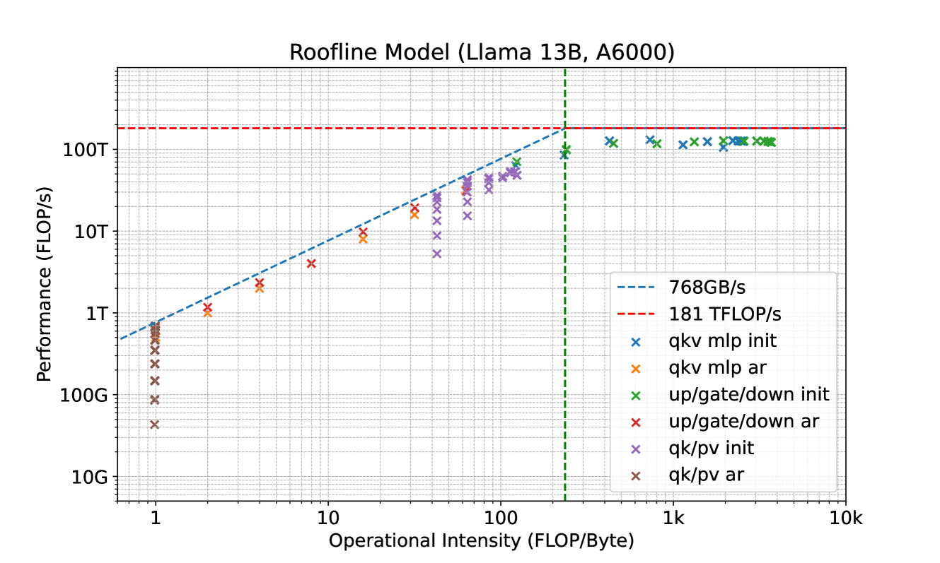
### Visual Description
# Technical Document Extraction: Roofline Model (Llama 13B, A6000)
## 1. Document Header
* **Title:** Roofline Model (Llama 13B, A6000)
* **Language:** English
## 2. Chart Specifications
This is a **Roofline Model** chart, a standard visualization used to represent the performance limits of a computing system (NVIDIA A6000 GPU) running a specific workload (Llama 13B model).
### Axis Definitions
* **Y-Axis (Vertical):** Performance (FLOP/s)
* **Scale:** Logarithmic (Base 10)
* **Range:** 10G to ~300T
* **Major Markers:** 10G, 100G, 1T, 10T, 100T
* **X-Axis (Horizontal):** Operational Intensity (FLOP/Byte)
* **Scale:** Logarithmic (Base 10)
* **Range:** ~0.6 to 10k
* **Major Markers:** 1, 10, 1k, 10k
### Legend and Thresholds
The legend is located in the bottom-right quadrant of the plot area.
| Legend Item | Color/Style | Description | Value/Threshold |
| :--- | :--- | :--- | :--- |
| **768GB/s** | Blue Dashed Line | Memory Bandwidth Limit (Slope) | 768 GB/s |
| **181 TFLOP/s** | Red Dashed Line | Peak Compute Performance (Ceiling) | 181 TFLOP/s |
| **qkv mlp init** | Blue 'x' | Data points for QKV/MLP initialization | High Intensity/High Perf |
| **qkv mlp ar** | Orange 'x' | Data points for QKV/MLP auto-regressive | Mid Intensity/Mid Perf |
| **up/gate/down init** | Green 'x' | Data points for Up/Gate/Down initialization | High Intensity/High Perf |
| **up/gate/down ar** | Red 'x' | Data points for Up/Gate/Down auto-regressive | Low Intensity/Low Perf |
| **qk/pv init** | Purple 'x' | Data points for QK/PV initialization | Mid Intensity/Mid Perf |
| **qk/pv ar** | Brown 'x' | Data points for QK/PV auto-regressive | Low Intensity/Low Perf |
---
## 3. Component Analysis
### The "Roofline" Structure
1. **Memory-Bound Region (The Slope):** Represented by the blue dashed line starting from the bottom left. It follows the formula $Performance = Bandwidth \times Intensity$. Any data point sitting on or near this line is limited by how fast data can be moved from memory (768 GB/s).
2. **Compute-Bound Region (The Ceiling):** Represented by the horizontal red dashed line at the top. It represents the hardware's maximum theoretical throughput (181 TFLOP/s).
3. **Ridge Point:** The intersection of the two lines occurs at an Operational Intensity of approximately **235 FLOP/Byte** (indicated by a vertical green dashed line).
### Data Series Trends and Distribution
* **Initialization (init) Phases:**
* **Trend:** These points (Blue, Green, Purple 'x') cluster toward the right side of the graph (High Operational Intensity).
* **Observation:** Most "init" points for `qkv mlp` and `up/gate/down` are located on the horizontal "ceiling," meaning they are compute-bound and utilizing the GPU's maximum TFLOP/s.
* **Auto-regressive (ar) Phases:**
* **Trend:** These points (Orange, Red, Brown 'x') cluster toward the left side of the graph (Low Operational Intensity).
* **Observation:** These points follow the diagonal blue dashed line. This indicates that the auto-regressive decoding phase of the Llama 13B model is strictly memory-bandwidth bound, operating significantly below the peak TFLOP/s of the A6000.
---
## 4. Data Point Extraction (Approximate Values)
| Category | Operational Intensity (FLOP/Byte) | Performance (FLOP/s) | Bottleneck |
| :--- | :--- | :--- | :--- |
| **up/gate/down ar** | ~1 to 10 | 100G to 5T | Memory (768GB/s) |
| **qk/pv ar** | ~1 (Vertical stack) | 40G to 800G | Memory (768GB/s) |
| **qkv mlp ar** | ~2 to 40 | 1T to 20T | Memory (768GB/s) |
| **qk/pv init** | ~40 to 150 | 10T to 80T | Transition/Memory |
| **qkv mlp init** | ~800 to 3k | ~150T to 181T | Compute (181 TFLOP/s) |
| **up/gate/down init** | ~200 to 4k | ~100T to 181T | Compute (181 TFLOP/s) |
## 5. Summary of Findings
The chart demonstrates that for a Llama 13B model on an A6000 GPU:
1. **Initialization** is highly efficient and hits the hardware's compute ceiling (181 TFLOP/s).
2. **Auto-regressive decoding** is inefficient in terms of raw compute utilization because it is bottlenecked by the 768 GB/s memory bandwidth.
3. The **qk/pv ar** (Brown 'x') operations are the least efficient, clustered at the lowest operational intensity (~1 FLOP/Byte).
</details>
Figure 16: Llama-13B operators on A6000.
<details>
<summary>x20.png Details</summary>
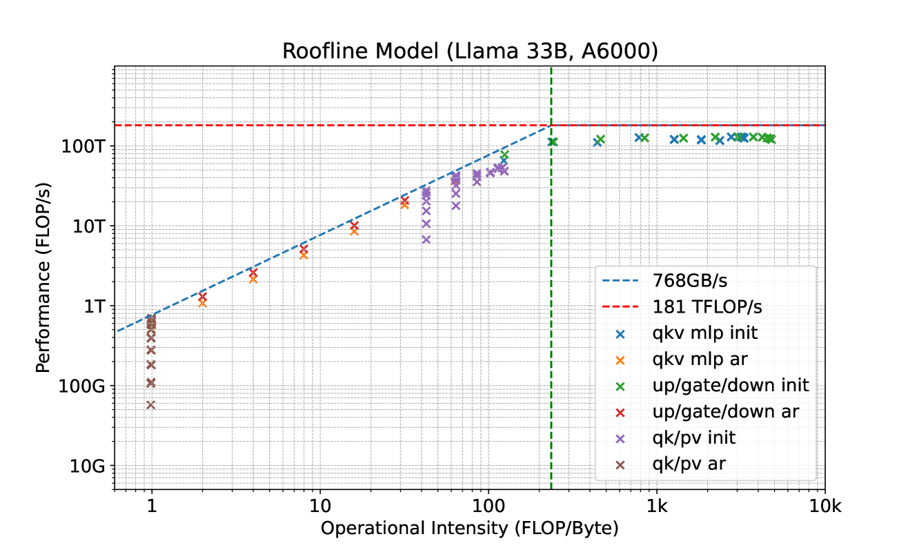
### Visual Description
# Technical Document Extraction: Roofline Model (Llama 33B, A6000)
## 1. Header Information
* **Title:** Roofline Model (Llama 33B, A6000)
* **Subject:** Performance analysis of a Llama 33B model running on an NVIDIA A6000 GPU.
## 2. Chart Specifications
The image is a **Roofline Chart**, a log-log plot used to visualize the performance limits of a computing system based on operational intensity.
### Axis Definitions
* **X-Axis (Horizontal):** Operational Intensity (FLOP/Byte)
* **Scale:** Logarithmic, ranging from approximately 0.6 to 10k.
* **Major Markers:** 1, 10, 100, 1k, 10k.
* **Y-Axis (Vertical):** Performance (FLOP/s)
* **Scale:** Logarithmic, ranging from 10G to roughly 500T.
* **Major Markers:** 10G, 100G, 1T, 10T, 100T.
### Legend and Thresholds
The legend is located in the bottom-right quadrant of the plot area.
| Label | Color/Style | Type | Value/Description |
| :--- | :--- | :--- | :--- |
| **768GB/s** | Blue Dashed Line | Slope | Memory Bandwidth Limit |
| **181 TFLOP/s** | Red Dashed Line | Horizontal | Peak Compute Performance |
| **qkv mlp init** | Blue 'x' | Data Series | Query/Key/Value MLP Initialization |
| **qkv mlp ar** | Orange 'x' | Data Series | Query/Key/Value MLP Auto-Regressive |
| **up/gate/down init** | Green 'x' | Data Series | Up/Gate/Down Projection Initialization |
| **up/gate/down ar** | Red 'x' | Data Series | Up/Gate/Down Projection Auto-Regressive |
| **qk/pv init** | Purple 'x' | Data Series | QK/PV Initialization |
| **qk/pv ar** | Brown 'x' | Data Series | QK/PV Auto-Regressive |
## 3. Component Analysis and Trends
### The "Roofline" Boundary
* **Memory-Bound Region:** Represented by the blue dashed diagonal line. It shows that for low operational intensity, performance is limited by the 768GB/s bandwidth.
* **Compute-Bound Region:** Represented by the red dashed horizontal line at 181 TFLOP/s. It shows the maximum theoretical throughput regardless of increased operational intensity.
* **Ridge Point:** The intersection occurs at an operational intensity of approximately **235 FLOP/Byte** (indicated by a vertical green dashed line).
### Data Series Trends
1. **Initialization (init) Series (Blue, Green, Purple):**
* **Trend:** These points cluster at the high end of the X-axis (Operational Intensity > 100).
* **Observation:** Most "init" tasks are compute-bound, sitting very close to the 181 TFLOP/s red line. The "up/gate/down init" (Green) and "qkv mlp init" (Blue) achieve the highest performance, nearly saturating the GPU's compute capacity.
2. **Auto-Regressive (ar) Series (Orange, Red, Brown):**
* **Trend:** These points slope upward from left to right, following the blue dashed diagonal line.
* **Observation:** These tasks are memory-bound. As the operational intensity increases (moving right), the performance increases linearly on the log-log scale until it hits the compute ceiling.
3. **qk/pv ar (Brown):**
* **Trend:** Vertical column at Operational Intensity = 1.
* **Observation:** This is the most memory-constrained task, showing a wide range of performance (from ~60G to ~800G FLOP/s) at a very low operational intensity.
## 4. Data Point Extraction (Approximate Values)
| Category | Operational Intensity (FLOP/Byte) | Performance (FLOP/s) | Regime |
| :--- | :--- | :--- | :--- |
| **up/gate/down init** | ~250 to ~5,000 | ~120T to ~150T | Compute-Bound |
| **qkv mlp init** | ~400 to ~4,000 | ~120T to ~140T | Compute-Bound |
| **qk/pv init** | ~40 to ~150 | ~7T to ~80T | Transition/Compute |
| **up/gate/down ar** | ~1 to ~40 | ~600G to ~20T | Memory-Bound |
| **qkv mlp ar** | ~2 to ~40 | ~1T to ~20T | Memory-Bound |
| **qk/pv ar** | ~1 | ~60G to ~800G | Memory-Bound |
## 5. Summary of Findings
The Llama 33B model on an A6000 GPU exhibits a clear distinction between initialization and auto-regressive phases. **Initialization** phases for large weight matrices (MLP and Up/Gate/Down) are highly efficient and **compute-bound**, operating near the 181 TFLOP/s limit. Conversely, **Auto-Regressive** phases are strictly **memory-bound**, with performance dictated by the 768 GB/s bandwidth limit, particularly for the QK/PV operations which reside at the lowest operational intensity.
</details>
Figure 17: Llama-33B operators on A6000.
G.2 FLOP/s vs. Operational Intensity Variations in Medusa
We investigate how Medusa can change Operational Intensity and elevate the FLOP/s. We choose Llama 33B on A100-80GB-PCIe as the setting.
First, we examine the attention matrix multiplication. Fig. 18 and Table 6 illustrate the effects of Medusa while keeping the batch size fixed at 16. We observe increased FLOP/s and Operational Intensity as more candidate tokens are added (original decoding results are plotted as grey dots). This indicates that Medusa can leverage additional candidate tokens to improve computational throughput. Compared to regular decoding, Medusa achieves 44 $×$ FLOP/s and 41 $×$ Operational Intensity under the setting of batch size 16 and sequence length 1024 with 64 candidate tokens. Fig. 19 and Table 7 illustrate the effects of Medusa decoding while keeping the sequence length fixed at 1024. Increasing the batch size does not improve Operational Intensity in this scenario.
Next, we examine the linear layer, focusing on the up/gate/down linear layers. The results are shown in Fig. 20 and Table 8. Since the linear layers in the decoding phase only process the future tokens while the past tokens are cached, they are independent of the sequence length. We vary the batch size to observe the effects. As Medusa increases the number of candidate tokens with the increasing batch size, we observe a shift from a memory-bandwidth-bound region to a computation-bound region. This shift demonstrates how Medusa can transition the performance characteristics of the linear layers from being limited by memory bandwidth to being limited by computational capacity.
<details>
<summary>x21.png Details</summary>
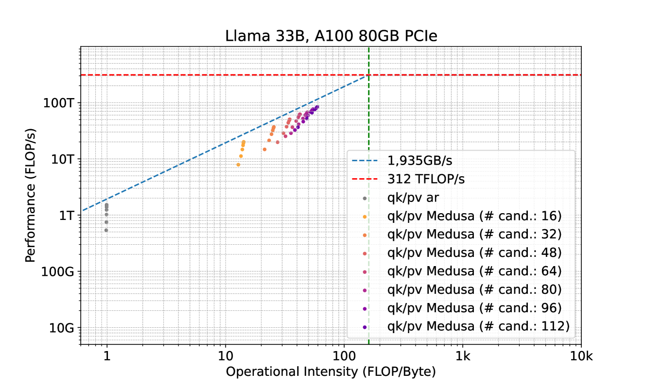
### Visual Description
# Technical Document Extraction: Roofline Model Analysis for Llama 33B
## 1. Header Information
* **Title:** Llama 33B, A100 80GB PCIe
* **Subject:** Performance analysis of a Llama 33B model on an NVIDIA A100 80GB PCIe GPU using a Roofline Model.
## 2. Chart Structure and Axes
The image is a **Roofline Chart**, which plots computational performance against operational intensity on a log-log scale.
* **Y-Axis (Performance):**
* **Label:** Performance (FLOP/s)
* **Scale:** Logarithmic, ranging from 10G to over 100T.
* **Major Markers:** 10G, 100G, 1T, 10T, 100T.
* **X-Axis (Operational Intensity):**
* **Label:** Operational Intensity (FLOP/Byte)
* **Scale:** Logarithmic, ranging from approximately 0.6 to 10k.
* **Major Markers:** 1, 10, 100, 1k, 10k.
## 3. Legend and Thresholds
The legend is located in the bottom-right quadrant of the plot area.
### Theoretical Limits (Lines)
* **Memory Bandwidth Limit (Blue Dashed Line):** Labeled as **1,935GB/s**. This line slopes upward from the bottom left, representing the maximum performance achievable based on memory throughput.
* **Compute Peak Limit (Red Dashed Line):** Labeled as **312 TFLOP/s**. This horizontal line represents the maximum theoretical floating-point performance of the hardware.
* **Ridge Point (Green Vertical Dashed Line):** This line marks the intersection of the memory limit and the compute limit, occurring at an operational intensity of approximately **161 FLOP/Byte** ($312 \times 10^{12} / 1935 \times 10^9$).
### Data Series (Scatter Points)
The data points represent different configurations of "qk/pv" (likely Query-Key/Projection-Value) operations.
* **Grey dots:** `qk/pv ar` (Autoregressive)
* **Orange dots:** `qk/pv Medusa (# cand.: 16)`
* **Light Orange/Tan dots:** `qk/pv Medusa (# cand.: 32)`
* **Salmon/Light Red dots:** `qk/pv Medusa (# cand.: 48)`
* **Pink/Magenta dots:** `qk/pv Medusa (# cand.: 64)`
* **Deep Pink dots:** `qk/pv Medusa (# cand.: 80)`
* **Purple dots:** `qk/pv Medusa (# cand.: 96)`
* **Dark Purple/Indigo dots:** `qk/pv Medusa (# cand.: 112)`
## 4. Data Analysis and Trends
### Component Isolation: Main Chart Area
The chart shows a clear progression of performance as the number of "candidates" (# cand.) increases in the Medusa configuration.
1. **Standard Autoregressive (`qk/pv ar`):**
* **Trend:** Clustered at the far left.
* **Placement:** Operational Intensity $\approx 1$ FLOP/Byte. Performance ranges between **0.5T and 1.5T FLOP/s**.
* **Observation:** This is heavily memory-bound, sitting far below the compute ceiling.
2. **Medusa Configurations (Colored Dots):**
* **Trend:** As the number of candidates increases (from 16 to 112), the data points move **up and to the right** along the memory bandwidth diagonal.
* **Operational Intensity Shift:** Moves from $\approx 13$ FLOP/Byte (16 candidates) to $\approx 60$ FLOP/Byte (112 candidates).
* **Performance Shift:** Moves from $\approx 8$T FLOP/s to nearly **100T FLOP/s**.
* **Efficiency:** All Medusa points track closely to the blue dashed line (1,935 GB/s), indicating that these operations are highly optimized for memory bandwidth but remain memory-bound (as they have not reached the horizontal red line).
### Summary Table of Extracted Data (Approximate Values)
| Configuration | Color | Approx. Op. Intensity (FLOP/Byte) | Approx. Performance (FLOP/s) |
| :--- | :--- | :--- | :--- |
| **qk/pv ar** | Grey | 1 | 0.5T - 1.5T |
| **Medusa 16** | Orange | 13 - 15 | 8T - 20T |
| **Medusa 32** | Light Orange | 22 - 28 | 15T - 35T |
| **Medusa 48** | Salmon | 30 - 35 | 25T - 50T |
| **Medusa 64** | Pink | 38 - 42 | 35T - 60T |
| **Medusa 80** | Deep Pink | 45 - 50 | 45T - 70T |
| **Medusa 96** | Purple | 52 - 58 | 55T - 80T |
| **Medusa 112** | Dark Purple | 60 - 65 | 65T - 90T |
## 5. Conclusion
The chart demonstrates that the Medusa optimization significantly increases the operational intensity of the Llama 33B model compared to standard autoregressive decoding. By increasing the number of candidates, the system achieves higher FLOP/s by moving further up the memory bandwidth limit line, though even at 112 candidates, the workload remains memory-bound on the A100 80GB PCIe.
</details>
Figure 18: FLOP/s vs. Operational Intensity of attention matrix multiplication with batch size 16.
<details>
<summary>x22.png Details</summary>
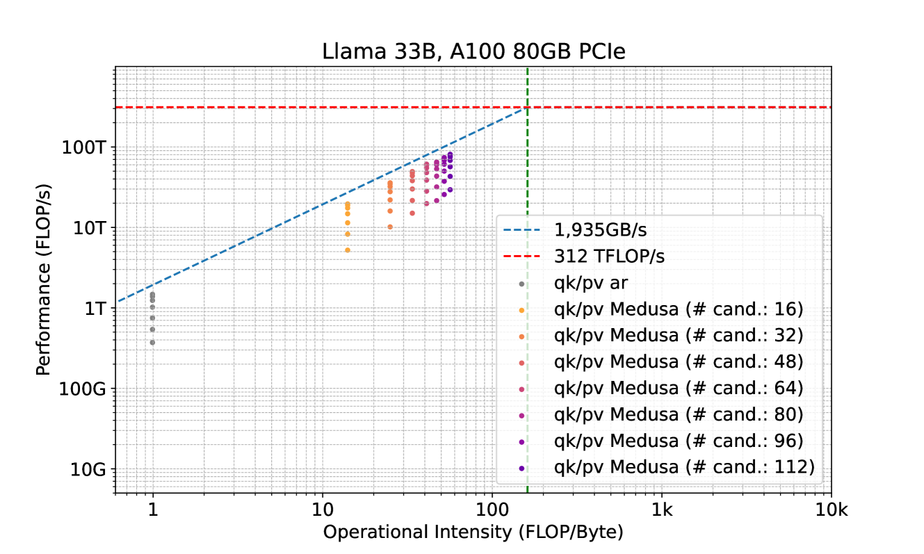
### Visual Description
# Technical Document Extraction: Roofline Model Analysis for Llama 33B
## 1. Document Header
* **Title:** Llama 33B, A100 80GB PCIe
* **Subject:** Performance analysis of a Large Language Model (Llama 33B) on specific hardware (NVIDIA A100 80GB PCIe) using a Roofline Model.
## 2. Chart Metadata and Axes
The image is a **Roofline Plot**, which relates computational performance to operational intensity. Both axes use a logarithmic scale.
* **Y-Axis (Performance):**
* **Label:** Performance (FLOP/s)
* **Scale:** Logarithmic, ranging from 10G to 100T+.
* **Major Markers:** 10G, 100G, 1T, 10T, 100T.
* **X-Axis (Operational Intensity):**
* **Label:** Operational Intensity (FLOP/Byte)
* **Scale:** Logarithmic, ranging from ~0.6 to 10k.
* **Major Markers:** 1, 10, 100, 1k, 10k.
## 3. Legend and Component Isolation
The legend is located in the lower-right quadrant of the main chart area.
### Hardware Limits (Lines)
* **Blue Dashed Diagonal Line:** Represents the memory bandwidth limit.
* **Label:** 1,935GB/s
* **Trend:** Slopes upward from left to right, indicating that at low operational intensity, performance is bound by memory transfer speeds.
* **Red Dashed Horizontal Line:** Represents the peak computational throughput.
* **Label:** 312 TFLOP/s
* **Trend:** Constant horizontal line at the top of the chart, indicating the hardware's maximum theoretical performance.
* **Green Dashed Vertical Line:** Represents the "Ridge Point" where the memory limit meets the compute limit. This occurs at an operational intensity of approximately 161 FLOP/Byte ($312 \times 10^{12} / 1935 \times 10^9$).
### Data Series (Scatter Points)
The data points represent different configurations of "qk/pv" (Query-Key/Projection-Value operations) for standard Autoregressive (ar) vs. Medusa decoding with varying candidate counts.
| Color | Label | Operational Intensity Range (Approx) | Performance Range (Approx) |
| :--- | :--- | :--- | :--- |
| **Grey** | qk/pv ar | ~1 FLOP/Byte | 400G - 1.5T FLOP/s |
| **Orange** | qk/pv Medusa (# cand.: 16) | ~15 FLOP/Byte | 5T - 20T FLOP/s |
| **Light Coral** | qk/pv Medusa (# cand.: 32) | ~25 FLOP/Byte | 10T - 35T FLOP/s |
| **Red-Pink** | qk/pv Medusa (# cand.: 48) | ~35 FLOP/Byte | 15T - 50T FLOP/s |
| **Deep Pink** | qk/pv Medusa (# cand.: 64) | ~45 FLOP/Byte | 20T - 65T FLOP/s |
| **Magenta** | qk/pv Medusa (# cand.: 80) | ~50 FLOP/Byte | 22T - 75T FLOP/s |
| **Purple** | qk/pv Medusa (# cand.: 96) | ~55 FLOP/Byte | 25T - 85T FLOP/s |
| **Dark Violet** | qk/pv Medusa (# cand.: 112) | ~60 FLOP/Byte | 30T - 90T FLOP/s |
## 4. Key Trends and Observations
1. **Memory Bound Regime:** All plotted data points fall significantly to the left of the green vertical ridge point. This indicates that the Llama 33B model on this hardware is **memory-bandwidth bound**, not compute-bound.
2. **Medusa Efficiency:** The standard autoregressive (ar) method (grey dots) has the lowest operational intensity (~1) and lowest performance.
3. **Scaling with Candidates:** As the number of Medusa candidates increases (from 16 to 112):
* The **Operational Intensity** increases (shifts right on the X-axis).
* The **Performance** increases (shifts up on the Y-axis).
* The data points follow the slope of the blue dashed line (1,935 GB/s), confirming that the performance gains are directly tied to utilizing more of the available memory bandwidth by increasing the work done per byte fetched.
4. **Performance Gap:** Even the highest performing Medusa configuration (~90 TFLOP/s) remains well below the theoretical peak of 312 TFLOP/s, as it is still constrained by the memory ceiling.
</details>
Figure 19: FLOP/s vs. Operational Intensity of attention matrix multiplication with sequence length 1024.
<details>
<summary>x23.png Details</summary>
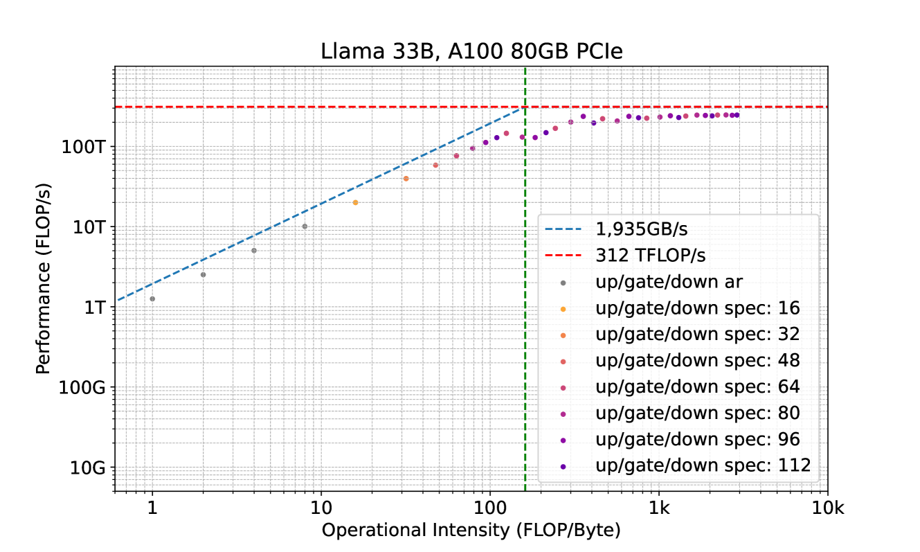
### Visual Description
# Technical Document Extraction: Roofline Model Analysis for Llama 33B on A100 80GB PCIe
## 1. Header Information
* **Title:** Llama 33B, A100 80GB PCIe
* **Subject:** Performance analysis of the Llama 33B model on a specific hardware configuration (NVIDIA A100 80GB PCIe GPU) using a Roofline Model.
## 2. Chart Structure and Axes
The image is a **Roofline Chart**, which plots computational performance against operational intensity on a log-log scale.
* **Y-Axis (Performance):**
* **Label:** Performance (FLOP/s)
* **Scale:** Logarithmic, ranging from 10G to 1000T (implied top).
* **Major Markers:** 10G, 100G, 1T, 10T, 100T.
* **X-Axis (Operational Intensity):**
* **Label:** Operational Intensity (FLOP/Byte)
* **Scale:** Logarithmic, ranging from 1 to 10k.
* **Major Markers:** 1, 10, 1k (1,000), 10k (10,000).
* **Grid:** Fine dashed grid lines for both axes to facilitate precise data reading.
## 3. Legend and Reference Lines
The legend is located in the bottom-right quadrant of the plot area.
### Reference Lines (The "Roofline")
* **Memory Bandwidth Ceiling (Blue Dashed Line):**
* **Label:** 1,935GB/s
* **Trend:** Slopes upward from left to right. It represents the maximum performance achievable when the operation is memory-bound.
* **Compute Peak Ceiling (Red Dashed Line):**
* **Label:** 312 TFLOP/s
* **Trend:** Horizontal line at the top of the chart. It represents the absolute hardware limit for floating-point operations per second.
* **Ridge Point (Green Vertical Dashed Line):**
* **Location:** Approximately 161 FLOP/Byte (where the blue and red lines intersect). This marks the transition from memory-bound to compute-bound regimes.
### Data Series (Scatter Points)
The points represent different execution configurations for "up/gate/down" operations.
* **Grey dots:** `up/gate/down ar` (Autoregressive)
* **Orange dots:** `up/gate/down spec: 16`
* **Light Orange/Tan dots:** `up/gate/down spec: 32`
* **Salmon dots:** `up/gate/down spec: 48`
* **Pink dots:** `up/gate/down spec: 64`
* **Magenta dots:** `up/gate/down spec: 80`
* **Purple dots:** `up/gate/down spec: 96`
* **Dark Purple dots:** `up/gate/down spec: 112`
## 4. Data Analysis and Trends
### Memory-Bound Region (Left of Green Line)
* **Trend:** Data points follow a linear upward trajectory (on the log-log scale) parallel to, but slightly below, the blue memory bandwidth ceiling.
* **Observations:**
* The `ar` (autoregressive) points (Grey) are at the lowest operational intensity (~1 to 10 FLOP/Byte) and lowest performance (~1T to 10T FLOP/s).
* As the "spec" value increases (from 16 to 112), the operational intensity increases, moving the points to the right.
* Performance increases proportionally with operational intensity in this region, indicating that the system is limited by how fast data can be moved from memory.
### Transition and Compute-Bound Region (Right of Green Line)
* **Trend:** As operational intensity exceeds ~200 FLOP/Byte, the performance curve flattens out, approaching the red dashed line (312 TFLOP/s).
* **Observations:**
* Points for `spec: 64` through `spec: 112` cluster at the top right.
* The highest performance achieved is approximately **250-280 TFLOP/s**, which is very close to the theoretical peak of 312 TFLOP/s.
* Increasing the "spec" value beyond 100 provides diminishing returns in performance as the hardware reaches its computational limit.
## 5. Summary of Key Data Points (Approximate)
| Configuration | Operational Intensity (FLOP/Byte) | Performance (FLOP/s) | Regime |
| :--- | :--- | :--- | :--- |
| **ar (Grey)** | ~1 - 8 | ~1.2T - 10T | Memory-Bound |
| **spec: 16 (Orange)** | ~16 | ~20T | Memory-Bound |
| **spec: 48 (Salmon)** | ~50 | ~60T | Memory-Bound |
| **spec: 80 (Magenta)** | ~120 | ~150T | Transition |
| **spec: 112 (Dk Purple)** | ~300 - 3000 | ~250T - 280T | Compute-Bound |
**Conclusion:** The chart demonstrates that for Llama 33B on an A100, standard autoregressive decoding is heavily memory-bound. Increasing the "spec" value (likely referring to speculative decoding or batching) significantly improves hardware utilization by increasing operational intensity until the 312 TFLOP/s compute ceiling is approached.
</details>
Figure 20: FLOP/s vs. Operational Intensity of Linear layers.
| 128 256 512 | 0.54 & 0.98 0.75 & 0.99 1.02 & 0.99 | 7.87 & 12.8 11.2 & 13.47 14.69 & 13.84 | 14.73 & 21.33 21.29 & 23.27 27.47 & 24.38 | 19.78 & 27.43 28.69 & 30.72 37.35 & 32.68 | 25.25 & 32.0 36.59 & 36.57 47.09 & 39.38 | 28.63 & 35.56 41.2 & 41.29 52.24 & 44.91 | 32.58 & 38.4 45.99 & 45.18 59.55 & 49.55 | 36.57 & 40.73 52.33 & 48.43 66.35 & 53.49 |
| --- | --- | --- | --- | --- | --- | --- | --- | --- |
| 1024 | 1.24 & 0.99 | 17.42 & 14.03 | 32.15 & 24.98 | 43.89 & 33.76 | 54.8 & 40.96 | 60.19 & 46.97 | 68.28 & 52.07 | 75.45 & 56.44 |
| 2048 | 1.39 & 0.99 | 19.03 & 14.12 | 35.05 & 25.28 | 48.03 & 34.32 | 59.66 & 41.8 | 63.91 & 48.08 | 72.83 & 53.43 | 80.05 & 58.04 |
| 4096 | 1.48 & 0.99 | 19.8 & 14.17 | 36.59 & 25.44 | 50.4 & 34.61 | 62.29 & 42.23 | 65.84 & 48.65 | 74.86 & 54.13 | 82.06 & 58.87 |
| 8192 | 1.53 & 0.99 | 20.08 & 14.2 | 36.89 & 25.52 | 50.44 & 34.76 | 62.11 & 42.45 | 67.5 & 48.94 | 76.97 & 54.49 | 84.5 & 59.3 |
Table 6: TFLOP/s & Operational Intensity of attention matrix multiplication with batch size 16 for Llama 33B on an A100 80GB PCIe.
| 1 2 4 | 0.37 & 0.99 0.54 & 0.99 0.75 & 0.99 | 5.22 & 14.03 8.25 & 14.03 11.41 & 14.03 | 10.15 & 24.98 16.0 & 24.98 21.97 & 24.98 | 15.02 & 33.76 21.62 & 33.76 30.02 & 33.76 | 19.79 & 40.96 28.24 & 40.96 38.71 & 40.96 | 21.52 & 46.97 31.84 & 46.97 43.41 & 46.97 | 25.65 & 52.07 37.49 & 52.07 50.06 & 52.07 | 29.4 & 56.44 43.04 & 56.44 56.77 & 56.44 |
| --- | --- | --- | --- | --- | --- | --- | --- | --- |
| 8 | 1.02 & 0.99 | 14.78 & 14.03 | 27.78 & 24.98 | 38.09 & 33.76 | 47.99 & 40.96 | 53.32 & 46.97 | 61.0 & 52.07 | 68.11 & 56.44 |
| 16 | 1.24 & 0.99 | 17.42 & 14.03 | 32.15 & 24.98 | 43.89 & 33.76 | 54.8 & 40.96 | 60.19 & 46.97 | 68.28 & 52.07 | 75.45 & 56.44 |
| 32 | 1.39 & 0.99 | 18.89 & 14.03 | 34.67 & 24.98 | 47.57 & 33.76 | 58.89 & 40.96 | 63.61 & 46.97 | 72.17 & 52.07 | 79.21 & 56.44 |
| 64 | 1.48 & 0.99 | 19.58 & 14.03 | 35.87 & 24.98 | 49.45 & 33.76 | 61.13 & 40.96 | 64.84 & 46.97 | 73.73 & 52.07 | 81.02 & 56.44 |
Table 7: TFLOP/s & Operational Intensity of attention matrix multiplication with sequence length 1024 for Llama 33B on an A100 80GB PCIe.
| 1 2 4 | 1.26 & 1.0 2.51 & 2.0 5.03 & 4.0 | 19.95 & 15.95 39.66 & 31.79 76.44 & 63.17 | 39.69 & 31.79 76.53 & 63.17 145.8 & 124.71 | 58.4 & 47.53 112.05 & 94.14 128.85 & 184.69 | 76.57 & 63.17 145.73 & 124.71 167.85 & 243.17 | 94.4 & 78.7 130.67 & 154.89 201.19 & 300.21 | 111.91 & 94.14 129.1 & 184.69 236.93 & 355.85 | 128.64 & 109.47 148.56 & 214.12 195.91 & 410.14 |
| --- | --- | --- | --- | --- | --- | --- | --- | --- |
| 8 | 10.06 & 7.99 | 145.72 & 124.71 | 168.26 & 243.17 | 236.83 & 355.85 | 221.11 & 463.14 | 207.79 & 565.44 | 236.95 & 663.07 | 227.8 & 756.36 |
| 16 | 19.96 & 15.95 | 168.35 & 243.17 | 221.41 & 463.14 | 237.5 & 663.07 | 224.71 & 845.59 | 232.49 & 1012.87 | 241.12 & 1166.74 | 229.25 & 1308.76 |
| 32 | 39.69 & 31.79 | 221.74 & 463.14 | 224.88 & 845.59 | 241.33 & 1166.74 | 239.02 & 1440.25 | 245.83 & 1675.97 | 243.55 & 1881.24 | 240.33 & 2061.59 |
| 64 | 76.57 & 63.17 | 225.19 & 845.59 | 239.2 & 1440.25 | 243.26 & 1881.24 | 246.16 & 2221.31 | 246.91 & 2491.55 | 244.52 & 2711.46 | 246.14 & 2893.91 |
Table 8: TFLOP/s & Operational Intensity of linear layers (up/gate/down) for Llama 33B on an A100 80GB PCIe.
G.3 Predicting Medusa Performance
We further employ a straightforward analytical model for the acceleration rate. The ablation study results in Sec. 3.3.1 indicate that the acceleration rate can be approximated by a simple logarithmic function. Using the results from Fig. 4(a), we model the curve as $\texttt{acc\_rate}=0.477\log(\texttt{num\_candidate})$ . We simulate the latency of one simplified block of the Llama-7B model (sequentially processing $XW_{Q}$ , $XW_{K}$ , $XW_{V}$ , $QK^{T}$ , $PV$ , $XW_{u}$ , $XW_{g}$ , $XW_{d}$ ) by first fixing the batch size at 1 and the sequence length at 1024. The candidate tokens are processed parallelly by constructing the tree attention described in Section 2.1.2. We omit the latency of the post-processing steps including verification and acceptance for Medusa since they introduce marginal overhead. Fig. 21 illustrates the simulated acceleration rate and speedup for different numbers of candidate tokens under these settings. As the number of candidate tokens increases, both the acceleration rate and speedup initially show improvements. However, beyond 64, the speedup starts to decline, indicating diminishing returns with further increases in candidate length. This aligns with the experimental results in Fig. 4(b) and suggests that there is an optimal range for the numbers of candidate tokens where Medusa provides the most significant performance gains.
We plot the simulated speedup under different batch size settings with a fixed sequence length of 1024 in Fig. 22. The results indicate that when the batch size exceeds 32, the speedup decreases and may even have a negative effect. This occurs because the linear layers shift from being memory-bandwidth-bound to computationally bound.
We conduct another experiment using a batch size of 4 and different sequence lengths. As shown in Fig. 23, the optimal number of candidate tokens remains relatively consistent across different sequence lengths. However, as the sequence length increases, the overall performance decreases. This performance drop is primarily due to the overhead from attention matrix multiplication, while the linear layer computation remains constant since the computation of linear layers is independent of the sequence length.
Our simulations show that the optimal number of candidate tokens is key for model scaling with Medusa, as benefits decrease beyond a certain range. Initially, increasing batch size improves performance through parallelism, but too large a batch size shifts linear layers from memory-bandwidth-bound to compute-bound, reducing speedup. Longer sequences increase attention matrix multiplication overhead, lowering performance, and emphasizing the need to optimize attention mechanisms. Effective model scaling requires balancing the number of candidate tokens, adjusting batch sizes to avoid compute-bound transitions, and enhancing attention mechanisms for longer sequences. These strategies ensure better resource utilization and higher performance, demonstrating the value of simulations in predicting performance and guiding acceleration strategy design.
<details>
<summary>x24.png Details</summary>
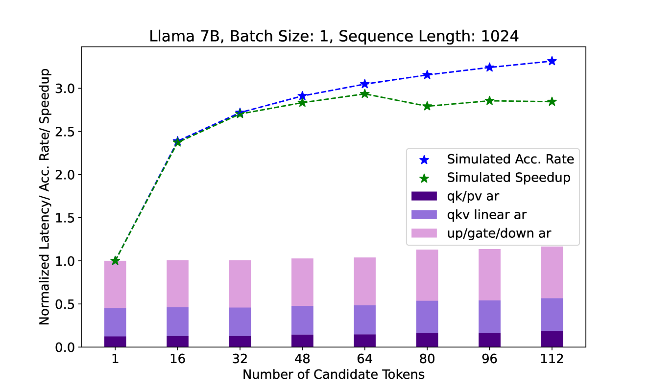
### Visual Description
# Technical Data Extraction: Llama 7B Performance Metrics
## 1. Document Metadata
* **Title:** Llama 7B, Batch Size: 1, Sequence Length: 1024
* **Primary Language:** English
* **Image Type:** Combined Line Graph and Stacked Bar Chart
## 2. Component Isolation
### A. Header
* **Text:** "Llama 7B, Batch Size: 1, Sequence Length: 1024"
* **Context:** Defines the model architecture and specific inference parameters used for the data collection.
### B. Main Chart Area (Axes)
* **Y-Axis Label:** "Normalized Latency/ Acc. Rate/ Speedup"
* **Y-Axis Scale:** Linear, ranging from 0.0 to 3.0+ (increments of 0.5).
* **X-Axis Label:** "Number of Candidate Tokens"
* **X-Axis Markers (Categories):** 1, 16, 32, 48, 64, 80, 96, 112.
### C. Legend
* **Blue Star ($\star$):** Simulated Acc. Rate (Line)
* **Green Star ($\star$):** Simulated Speedup (Line)
* **Dark Purple Block:** qk/pv ar (Stacked Bar component)
* **Medium Purple Block:** qkv linear ar (Stacked Bar component)
* **Light Pink/Lavender Block:** up/gate/down ar (Stacked Bar component)
---
## 3. Data Series Analysis & Trend Verification
### Series 1: Simulated Acc. Rate (Blue Star / Dashed Blue Line)
* **Visual Trend:** Consistent upward slope. The rate of increase is steepest between 1 and 32 tokens, then continues to climb at a shallower, steady gradient through to 112 tokens.
* **Estimated Data Points:**
* 1: ~1.0
* 16: ~2.4
* 32: ~2.7
* 48: ~2.9
* 64: ~3.05
* 80: ~3.15
* 96: ~3.25
* 112: ~3.3
### Series 2: Simulated Speedup (Green Star / Dashed Green Line)
* **Visual Trend:** Initial rapid growth matching the Acc. Rate until 32 tokens. It plateaus between 64 and 112 tokens, showing a slight dip at 80 before stabilizing.
* **Estimated Data Points:**
* 1: 1.0 (Baseline)
* 16: ~2.4
* 32: ~2.7
* 48: ~2.85
* 64: ~2.95
* 80: ~2.8
* 96: ~2.85
* 112: ~2.85
### Series 3: Normalized Latency Components (Stacked Bars)
* **Visual Trend:** The total height of the bars (representing total normalized latency) remains very close to 1.0 for candidate tokens 1 through 64. Starting at 80 tokens, the total latency begins to increase visibly, reaching approximately 1.2 by 112 tokens.
* **Component Breakdown:**
* **qk/pv ar (Dark Purple):** Smallest contributor; remains relatively constant with a very slight increase as token count grows.
* **qkv linear ar (Medium Purple):** Middle contributor; remains stable until 80 tokens, where it expands slightly.
* **up/gate/down ar (Light Pink):** Largest contributor; remains stable until 80 tokens, then shows the most significant growth in height, driving the overall latency increase.
---
## 4. Data Table Reconstruction (Estimated Values)
| Number of Candidate Tokens | Simulated Acc. Rate (Blue) | Simulated Speedup (Green) | Total Normalized Latency (Bar Height) |
| :--- | :--- | :--- | :--- |
| **1** | 1.0 | 1.0 | 1.0 |
| **16** | 2.4 | 2.4 | 1.0 |
| **32** | 2.7 | 2.7 | 1.0 |
| **48** | 2.9 | 2.85 | 1.02 |
| **64** | 3.05 | 2.95 | 1.04 |
| **80** | 3.15 | 2.8 | 1.13 |
| **96** | 3.25 | 2.85 | 1.15 |
| **112** | 3.3 | 2.85 | 1.18 |
---
## 5. Technical Summary
The chart illustrates the performance of a Llama 7B model using speculative decoding or a similar candidate-token-based acceleration method.
* **Efficiency Peak:** The "Simulated Speedup" tracks closely with the "Simulated Acceptance Rate" until approximately 32-48 candidate tokens.
* **Diminishing Returns:** Beyond 64 tokens, the "Simulated Speedup" plateaus and even slightly regresses. This is explained by the "Normalized Latency" bars, which show that the computational overhead (specifically in the `up/gate/down` and `qkv linear` layers) begins to increase significantly after 64 tokens, offsetting the gains from a higher acceptance rate.
</details>
Figure 21: Simulated acceleration rate, speedup, and normalized latency ablation using different numbers of candidate tokens under the setting of batch size 1 and sequence length 1024 for Llama-7B on an A100 80GB PCIe.
<details>
<summary>x25.png Details</summary>
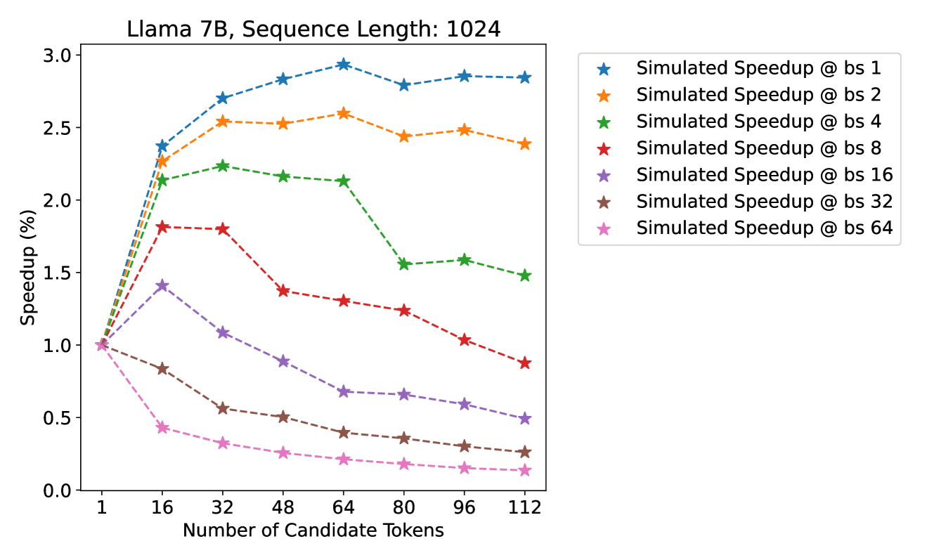
### Visual Description
# Technical Document Extraction: Llama 7B Performance Analysis
## 1. Header Information
* **Title:** Llama 7B, Sequence Length: 1024
* **Primary Subject:** Simulated Speedup performance relative to the number of candidate tokens across various batch sizes (bs).
## 2. Chart Metadata and Axes
* **Chart Type:** Multi-series line graph with markers.
* **X-Axis Label:** Number of Candidate Tokens
* **Markers:** 1, 16, 32, 48, 64, 80, 96, 112
* **Y-Axis Label:** Speedup (%)
* **Range:** 0.0 to 3.0
* **Markers:** 0.0, 0.5, 1.0, 1.5, 2.0, 2.5, 3.0
* **Legend Location:** Right-hand side, external to the main plot area.
* **Legend Content:**
* ★ (Blue): Simulated Speedup @ bs 1
* ★ (Orange): Simulated Speedup @ bs 2
* ★ (Green): Simulated Speedup @ bs 4
* ★ (Red): Simulated Speedup @ bs 8
* ★ (Purple): Simulated Speedup @ bs 16
* ★ (Brown): Simulated Speedup @ bs 32
* ★ (Pink): Simulated Speedup @ bs 64
---
## 3. Data Series Analysis and Trends
All series originate at a Speedup of **1.0** when the Number of Candidate Tokens is **1**.
### Series 1: Simulated Speedup @ bs 1 (Blue Line)
* **Trend:** Sharp upward slope initially, peaking at 64 tokens, followed by a slight plateau/minor fluctuation.
* **Key Data Points (Approximate):**
* 16 tokens: ~2.35
* 64 tokens: ~2.95 (Peak)
* 112 tokens: ~2.85
### Series 2: Simulated Speedup @ bs 2 (Orange Line)
* **Trend:** Strong upward slope, peaking at 64 tokens, then a slight decline and stabilization.
* **Key Data Points (Approximate):**
* 16 tokens: ~2.25
* 64 tokens: ~2.60 (Peak)
* 112 tokens: ~2.40
### Series 3: Simulated Speedup @ bs 4 (Green Line)
* **Trend:** Upward slope peaking early at 32 tokens, maintaining a plateau until 64, then a significant drop at 80 tokens.
* **Key Data Points (Approximate):**
* 32 tokens: ~2.25 (Peak)
* 64 tokens: ~2.15
* 80 tokens: ~1.55
* 112 tokens: ~1.50
### Series 4: Simulated Speedup @ bs 8 (Red Line)
* **Trend:** Initial increase peaking at 16-32 tokens, followed by a steady downward slope as candidate tokens increase.
* **Key Data Points (Approximate):**
* 16 tokens: ~1.80 (Peak)
* 32 tokens: ~1.80
* 64 tokens: ~1.30
* 112 tokens: ~0.90 (Drops below baseline)
### Series 5: Simulated Speedup @ bs 16 (Purple Line)
* **Trend:** Slight initial increase peaking at 16 tokens, followed by a consistent downward trend.
* **Key Data Points (Approximate):**
* 16 tokens: ~1.40 (Peak)
* 64 tokens: ~0.70
* 112 tokens: ~0.50
### Series 6: Simulated Speedup @ bs 32 (Brown Line)
* **Trend:** Immediate and continuous downward slope from the baseline.
* **Key Data Points (Approximate):**
* 16 tokens: ~0.85
* 64 tokens: ~0.40
* 112 tokens: ~0.25
### Series 7: Simulated Speedup @ bs 64 (Pink Line)
* **Trend:** Sharp immediate downward slope, representing the lowest performance across all configurations.
* **Key Data Points (Approximate):**
* 16 tokens: ~0.45
* 64 tokens: ~0.20
* 112 tokens: ~0.15
---
## 4. Component Isolation & Summary
* **Header:** Defines the model (Llama 7B) and context (1024 sequence length).
* **Main Chart:** Visualizes the inverse relationship between batch size and speedup efficiency as candidate tokens increase.
* **Key Observation:** Lower batch sizes (bs 1, 2, 4) benefit significantly from increasing candidate tokens, achieving up to ~3x speedup. Conversely, higher batch sizes (bs 16, 32, 64) see a performance degradation (speedup < 1.0) as the number of candidate tokens increases, suggesting overhead costs outweigh the benefits of speculative execution at high concurrency.
</details>
Figure 22: Simulated speedup with sequence length 1024 for Llama-7B.
<details>
<summary>x26.png Details</summary>
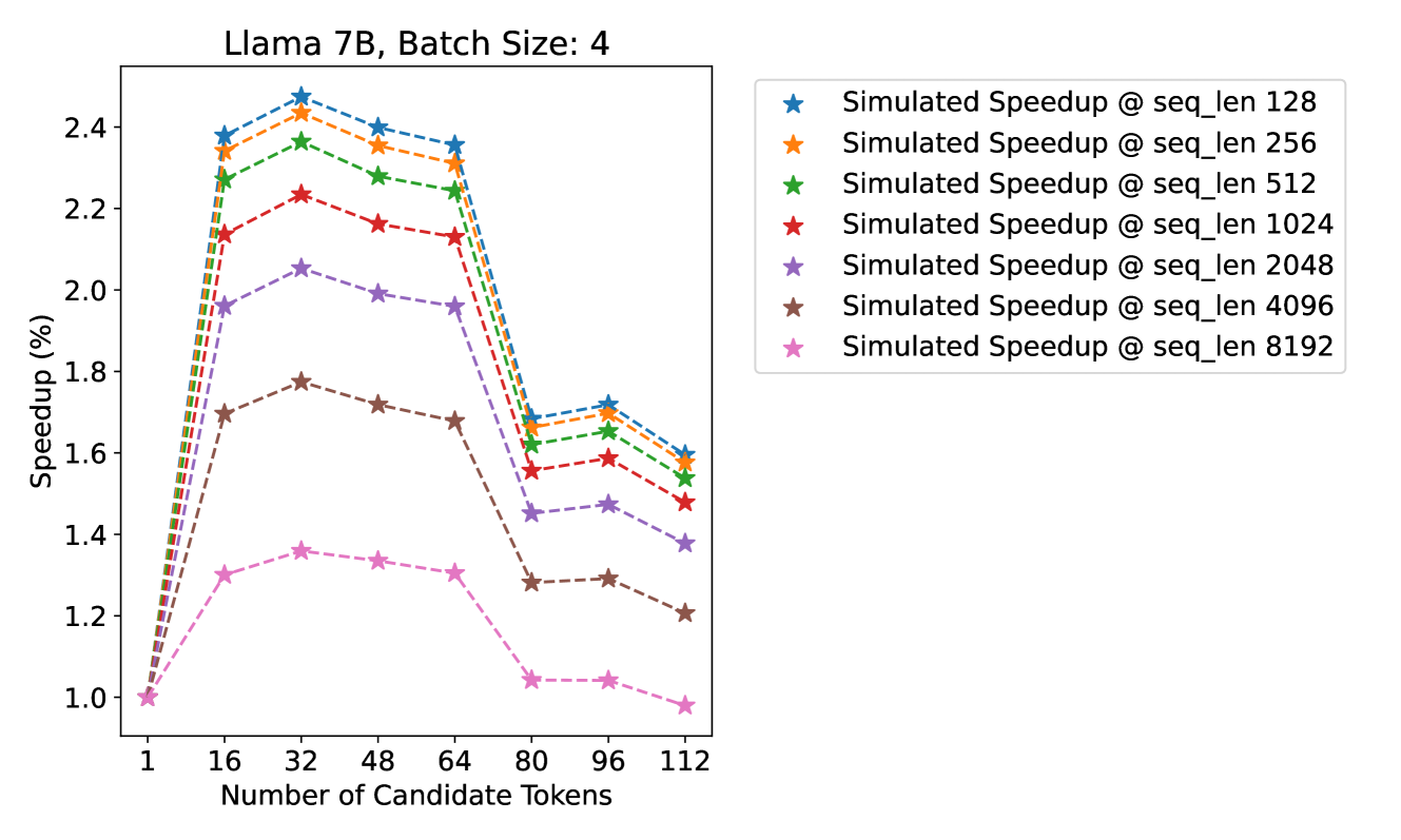
### Visual Description
# Technical Document Extraction: Llama 7B Performance Analysis
## 1. Header Information
* **Title:** Llama 7B, Batch Size: 4
* **Primary Subject:** Simulated Speedup performance relative to the number of candidate tokens across various sequence lengths.
## 2. Component Isolation
### A. Axis Definitions
* **Y-Axis (Vertical):**
* **Label:** Speedup (%)
* **Scale:** Linear, ranging from 1.0 to 2.4 (increments of 0.2 marked).
* **X-Axis (Horizontal):**
* **Label:** Number of Candidate Tokens
* **Markers (Ticks):** 1, 16, 32, 48, 64, 80, 96, 112.
### B. Legend (Spatial Placement: Top Right [x=0.55 to 0.95, y=0.55 to 0.90])
The legend identifies seven data series, all represented by star markers connected by dashed lines.
1. **Blue Star:** Simulated Speedup @ seq_len 128
2. **Orange Star:** Simulated Speedup @ seq_len 256
3. **Green Star:** Simulated Speedup @ seq_len 512
4. **Red Star:** Simulated Speedup @ seq_len 1024
5. **Purple Star:** Simulated Speedup @ seq_len 2048
6. **Brown Star:** Simulated Speedup @ seq_len 4096
7. **Pink Star:** Simulated Speedup @ seq_len 8192
---
## 3. Trend Verification and Data Extraction
### General Visual Trend
All data series follow a consistent geometric pattern:
1. **Initial Surge:** A sharp upward slope from 1 to 16 candidate tokens.
2. **Peak Performance:** Reaching a maximum at 32 candidate tokens.
3. **Gradual Decline:** A slight downward slope between 32 and 64 tokens.
4. **Significant Drop:** A sharp vertical decline between 64 and 80 tokens.
5. **Secondary Peak/Plateau:** A minor recovery or stabilization between 80 and 96 tokens.
6. **Final Decline:** A downward slope toward 112 tokens.
7. **Inverse Correlation:** Speedup is inversely proportional to sequence length; shorter sequences (e.g., 128) consistently outperform longer sequences (e.g., 8192).
### Data Table (Estimated Values)
All series start at a baseline of **1.0 Speedup** at **1 Candidate Token**.
| Number of Candidate Tokens | seq_len 128 (Blue) | seq_len 256 (Orange) | seq_len 512 (Green) | seq_len 1024 (Red) | seq_len 2048 (Purple) | seq_len 4096 (Brown) | seq_len 8192 (Pink) |
| :--- | :---: | :---: | :---: | :---: | :---: | :---: | :---: |
| **1** | 1.00 | 1.00 | 1.00 | 1.00 | 1.00 | 1.00 | 1.00 |
| **16** | ~2.38 | ~2.34 | ~2.27 | ~2.14 | ~1.96 | ~1.70 | ~1.30 |
| **32 (Peak)** | **~2.48** | **~2.44** | **~2.37** | **~2.24** | **~2.06** | **~1.78** | **~1.36** |
| **48** | ~2.40 | ~2.36 | ~2.28 | ~2.16 | ~1.99 | ~1.72 | ~1.34 |
| **64** | ~2.36 | ~2.32 | ~2.24 | ~2.13 | ~1.96 | ~1.68 | ~1.31 |
| **80 (Drop)** | ~1.68 | ~1.66 | ~1.62 | ~1.56 | ~1.45 | ~1.28 | ~1.04 |
| **96** | ~1.72 | ~1.70 | ~1.66 | ~1.59 | ~1.48 | ~1.29 | ~1.04 |
| **112** | ~1.60 | ~1.58 | ~1.54 | ~1.48 | ~1.38 | ~1.21 | ~0.98 |
---
## 4. Key Observations
* **Optimal Configuration:** For all sequence lengths, the "Number of Candidate Tokens" value of **32** yields the highest speedup.
* **Performance Ceiling:** The maximum speedup achieved is approximately **2.48x (248%)** for the shortest sequence length (128) at 32 candidate tokens.
* **Efficiency Threshold:** There is a critical performance "cliff" after 64 candidate tokens. The speedup drops by approximately 0.6x to 0.7x across most series when moving from 64 to 80 tokens, suggesting a hardware or architectural bottleneck (likely memory or cache related) triggered at that specific token count.
* **Long Sequence Penalty:** At a sequence length of 8192, the speedup barely stays above 1.0 and actually dips slightly below the baseline (to ~0.98) at 112 candidate tokens, indicating that the overhead of candidate tokens outweighs the benefits for very long sequences at high token counts.
</details>
Figure 23: Simulated speedup with batch size 4 for Llama-7B.