# Distributionally Robust Receive Combining
**Authors**: Shixiong Wang, Wei Dai, and Geoffrey Ye Li
> S. Wang, W. Dai, and G. Li are with the Department of Electrical and Electronic Engineering, Imperial College London, London SW7 2AZ, United Kingdom (E-mail: This work is supported by the UK Department for Science, Innovation and Technology under the Future Open Networks Research Challenge project TUDOR (Towards Ubiquitous 3D Open Resilient Network).
## Abstract
This article investigates signal estimation in wireless transmission (i.e., receive combining) from the perspective of statistical machine learning, where the transmit signals may be from an integrated sensing and communication system; that is, 1) signals may be not only discrete constellation points but also arbitrary complex values; 2) signals may be spatially correlated. Particular attention is paid to handling various uncertainties such as the uncertainty of the transmit signal covariance, the uncertainty of the channel matrix, the uncertainty of the channel noise covariance, the existence of channel impulse noises, the non-ideality of the power amplifiers, and the limited sample size of pilots. To proceed, a distributionally robust receive combining framework that is insensitive to the above uncertainties is proposed, which reveals that channel estimation is not a necessary operation. For optimal linear estimation, the proposed framework includes several existing combiners as special cases such as diagonal loading and eigenvalue thresholding. For optimal nonlinear estimation, estimators are limited in reproducing kernel Hilbert spaces and neural network function spaces, and corresponding uncertainty-aware solutions (e.g., kernelized diagonal loading) are derived. In addition, we prove that the ridge and kernel ridge regression methods in machine learning are distributionally robust against diagonal perturbation in feature covariance.
Index Terms: Wireless Transmission, Smart Antenna, Machine Learning, Robust Estimation, Robust Combining, Distributional Uncertainty, Channel Uncertainty, Limited Pilot.
## I Introduction
In wireless transmission, detection and estimation of transmitted signals is of high importance, and combining at array receivers serves as a key signal-processing technique to suppress interference and environmental noises. The earliest beamforming solutions rely on the use of phase shifters (e.g., phased arrays) to steer and shape wave lobes, while advanced combining methods allow the employment of digital signal processing units, which introduce additional structural freedom (e.g., fully digital, hybrid, nonlinear, wideband) in combiner design and significant performance improvement in signal recovery [1, 2, 3].
In traditional communication systems, transmitted signals are discrete points from constellations. Therefore, signal recovery, commonly referred to as signal detection, can be cast into a classification problem from the perspective of statistical machine learning, and the number of candidate classes is determined by the number of points in the employed constellation. Research in this stream includes, e.g., [4, 5, 6, 7, 8, 9] as well as references therein, and the performance measure for signal detection is usually the misclassification rate (i.e., symbol error rate); representative algorithms encompass the maximum likelihood detector, the sphere decoding, etc. In another research stream, the signal recovery performance is evaluated using mean-squared errors (cf., signal-to-interference-plus-noise ratio), and the resultant signal recovery problem is commonly known as signal estimation, which can be considered as a regression problem from the perspective of statistical machine learning. By comparing the estimated symbols with the constellation points afterward, the detection of discrete symbols can be realized. For this case, till now, typical combining solutions include zero-forcing receivers, Wiener receivers (i.e., linear minimum mean-squared error receivers), Capon receivers (i.e., minimum variance distortionless response receivers), and nonlinear receivers such as neural-network receivers [10, 11, 12]. On the basis of these canonical approaches, variants such as robust beamformers working against the limited size of pilot samples and the uncertainty in steering vectors [13, 14, 15, 16, 17, 18] have also been intensively reported; among these robust solutions, the diagonal loading method [19], [14, Eq. (11)] and the eigenvalue thresholding method [20], [14, Eq. (12)] are popular due to their excellent balance between practical performance and technical simplicity.
Different from traditional paradigms, in emerging communication systems, e.g., integrated sensing and communication (ISAC) systems, transmitted signals may be arbitrary complex values and spatially correlated [21, 22, 23]. As a result, mean-squared error is a preferred performance measure to investigate the receive combining and estimation problem of wireless signals, which is, therefore, the focus of this article.
Although a large body of problems have been attacked in the area, the following signal-processing problems of combining and estimation in wireless transmission remain unsolved.
1. What is the relation between the signal-model-based approaches (e.g., Wiener and Capon receivers) and the data-driven approaches (e.g., deep-learning receivers)? In other words, how can we build a mathematically unified modeling framework to interpret all the existing digital receive combiners?
1. In addition to the limited pilot size and the uncertainty in steering vectors, there exist other uncertainties in the signal model: the uncertainty of the transmit signal covariance, the uncertainty of the communication channel matrix, the uncertainty of the channel noise covariance, the presence of channel impulse noises (i.e., outliers), and the non-ideality of the power amplifiers. Therefore, how can we handle all these types of uncertainties in a unified solution framework?
1. Existing literature mainly studied the robustness theory of linear beamformers against limited pilot size and the uncertainty in steering vectors [13, 14, 15, 16, 17, 18]. However, how can we develop the theory of robust nonlinear combiners against all the aforementioned uncertainties?
To this end, this article designs a unified modeling and solution framework for receive combining of wireless signals, in consideration of the scarcity of the pilot data and the different uncertainties in the signal model.
### I-A Contributions
The contributions of this article can be summarized from the aspects of machine learning theory and wireless transmission theory.
In terms of machine learning theory, we give a justification of the popular ridge regression and kernel ridge regression (i.e., quadratic loss function plus squared- $F$ -norm regularization) from the perspective of distributional robustness against diagonal perturbation in feature covariance, which enriches the theory of trustworthy machine learning; see Theorems 2 and 3, as well as Corollaries 3 and 5.
In terms of wireless transmission theory, the contributions are outlined below.
1. We build a fundamentally theoretical framework for receive combining from the perspective of statistical machine learning. In addition to the linear estimation methods, nonlinear approaches (i.e., nonlinear combining) are also discussed in reproducing kernel Hilbert spaces and neural network function spaces. In particular, we reveal that channel estimation is not a necessary operation in receive combining. For details, see Subsection III-A.
1. The presented framework is particularly developed from the perspective of distributional robustness which can therefore combat the limited size of pilot data and several types of uncertainties in the wireless signal model such as the uncertainty in the transmit power matrix, the uncertainty in the communication channel matrix, the existence of channel impulse noises (i.e., outliers), the uncertainty in the covariance matrix of channel noises, the non-ideality of the power amplifiers, etc. For details, see Subsection III-B, and the technical developments in Sections IV and V.
1. Existing methods such as diagonal loading and eigenvalue thresholding are proven to be distributionally robust against the limited pilot size and all the aforementioned uncertainties in the wireless signal model. Extensions of diagonal loading and eigenvalue thresholding are proposed as well. Moreover, the kernelized diagonal loading and the kernelized eigenvalue thresholding methods are put forward for nonlinear estimation cases. For details, see Corollary 1, Examples 4 and 5, and Subsections IV-B.
1. The distributionally robust receive combining and signal estimation problems across multiple frames, where channel conditions may change, are also investigated. For details, see Subsections IV-C and V-A 2.
### I-B Notations
The $N$ -dimensional real (coordinate) space and complex (coordinate) space are denoted as $\mathbb{R}^{N}$ and $\mathbb{C}^{N}$ , respectively. Lowercase symbols (e.g., $\bm{x}$ ) denote vectors (column by default) and uppercase ones (e.g., $\bm{X}$ ) denote matrices. We use the Roman font for random quantities (e.g., $\mathbf{x},\mathbf{X}$ ) and the italic font for deterministic quantities (e.g., $\bm{x},\bm{X}$ ). Let $\operatorname{Re}\bm{X}$ be the real part of a complex quantity $\bm{X}$ (a vector or matrix) and $\operatorname{Im}\bm{X}$ be the imaginary part of $\bm{X}$ . For a vector $\bm{x}\in\mathbb{C}^{N}$ , let
$$
\underline{\bm{x}}\coloneqq\left[\begin{array}[]{cc}\operatorname{Re}\bm{x}\\
\operatorname{Im}\bm{x}\end{array}\right]\in\mathbb{R}^{2N}
$$
be the real-space representation of $\bm{x}$ ; for a matrix $\bm{H}\in\mathbb{C}^{N\times M}$ , let
$$
\underline{\bm{H}}\coloneqq\left[\begin{array}[]{cc}\operatorname{Re}\bm{H}\\
\operatorname{Im}\bm{H}\end{array}\right],~{}~{}~{}~{}~{}\underline{\underline
{\bm{H}}}\coloneqq\left[\begin{array}[]{cc}\operatorname{Re}\bm{H}&-
\operatorname{Im}\bm{H}\\
\operatorname{Im}\bm{H}&\operatorname{Re}\bm{H}\end{array}\right]
$$
be the real-space representations of $\bm{H}$ where $\underline{\bm{H}}\in\mathbb{R}^{2N\times M}$ and $\underline{\underline{\bm{H}}}\in\mathbb{R}^{2N\times 2M}$ . The running index set induced by an integer $N$ is defined as $[N]\coloneqq\{1,2,\ldots,N\}$ . To concatenate matrices and vectors, MATLAB notations are used: i.e., $[\bm{A},~{}\bm{B}]$ for row stacking and $[\bm{A};~{}\bm{B}]$ for column stacking. We let $\bm{\Gamma}_{M}\coloneqq[\bm{I}_{M},~{}\bm{J}_{M}]\in\mathbb{C}^{M\times 2M}$ where $\bm{I}_{M}$ denotes the $M$ -dimensional identity matrix, $\bm{J}_{M}\coloneqq j\cdot\bm{I}_{M}$ , and $j$ denotes the imaginary unit. Let $\mathcal{N}(\bm{\mu},\bm{\Sigma})$ denote a real Gaussian distribution with mean $\bm{\mu}$ and covariance $\bm{\Sigma}$ . We use $\mathcal{CN}(\bm{s},\bm{P},\bm{C})$ to denote a complex Gaussian distribution with mean $\bm{s}$ , covariance $\bm{P}$ , and pseudo-covariance $\bm{C}$ ; if $\bm{C}$ is not specified, we imply $\bm{C}=\bm{0}$ .
## II Preliminaries
We review two popular structured representation methods of nonlinear functions $\bm{\phi}:\mathbb{R}^{N}\to\mathbb{R}^{M}$ . More details can be seen in Appendix A.
### II-A Reproducing Kernel Hilbert Spaces
A reproducing kernel Hilbert space (RKHS) $\mathcal{H}$ induced by the kernel function $\ker:\mathbb{R}^{N}\times\mathbb{R}^{N}\to\mathbb{R}$ and a collection of points $\{\bm{x}_{1},\bm{x}_{2},\ldots,\bm{x}_{L}\}\subset\mathbb{R}^{N}$ is a set of functions from $\mathbb{R}^{N}$ to $\mathbb{R}$ ; $L$ may be infinite. Every function $\phi:\mathbb{R}^{N}\to\mathbb{R}$ in the functional space $\mathcal{H}$ can be represented by a linear combination [24, p. 539; Chap. 14]
$$
\phi(\bm{x})=\sum^{L}_{i=1}\omega_{i}\cdot\ker(\bm{x},\bm{x}_{i}),~{}\forall
\bm{x}\in\mathbb{R}^{N} \tag{1}
$$
where $\{\omega_{i}\}_{i\in[L]}$ are the combination weights; $\omega_{i}\in\mathbb{R}$ for every $i\in[L]$ . The matrix form of (1) for $M$ -multiple functions are
$$
\bm{\phi}(\bm{x})\coloneqq\left[\begin{array}[]{ccccccc}\phi_{1}(\bm{x})\\
\phi_{2}(\bm{x})\\
\vdots\\
\phi_{M}(\bm{x})\end{array}\right]=\bm{W}\cdot\bm{\varphi}(\bm{x})\coloneqq
\left[\begin{array}[]{c}\bm{\omega}_{1}\\
\bm{\omega}_{2}\\
\vdots\\
\bm{\omega}_{M}\end{array}\right]\cdot\bm{\varphi}(\bm{x}), \tag{2}
$$
where $\bm{\omega}_{1},\bm{\omega}_{2},\ldots,\bm{\omega}_{M}\in\mathbb{R}^{L}$ are weight row-vectors for functions $\phi_{1}(\bm{x}),\phi_{2}(\bm{x}),\ldots,\phi_{M}(\bm{x})$ , respectively, and
$$
\bm{W}\coloneqq\left[\begin{array}[]{c}\bm{\omega}_{1}\\
\bm{\omega}_{2}\\
\vdots\\
\bm{\omega}_{M}\end{array}\right]\in\mathbb{R}^{M\times L},~{}~{}~{}\bm{
\varphi}(\bm{x})\coloneqq\left[\begin{array}[]{c}\ker(\bm{x},\bm{x}_{1})\\
\ker(\bm{x},\bm{x}_{2})\\
\vdots\\
\ker(\bm{x},\bm{x}_{L})\end{array}\right]. \tag{3}
$$
Since a kernel function is pre-designed (i.e., fixed) for an RKHS $\mathcal{H}$ , (2) suggests a $\bm{W}$ -linear representation of $\bm{x}$ -nonlinear functions $\bm{\phi}(\bm{x})$ in $\mathcal{H}^{M}$ . Note that there exists a one-to-one correspondence between $\bm{\phi}$ and $\bm{W}$ : for every $\bm{\phi}:\mathbb{R}^{N}\to\mathbb{R}^{M}$ , there exists a $\bm{W}\in\mathbb{R}^{M\times L}$ , and vice versa.
### II-B Neural Networks
Neural networks (NN) are another powerful tool to represent (i.e., approximate) nonlinear functions. A neural network function space (NNFS) $\mathcal{K}$ characterizes (or parameterizes) a set of multi-input multi-output functions. Typical choices are multi-layer feed-forward neural networks, recurrent neural networks, etc. For combining and estimation of wireless signals, the multi-layer feed-forward neural networks are standard [10, 11, 12]. Suppose that we have $R-1$ hidden layers (so in total $R+1$ layers including one input layer and one output layer) and each layer $r=0,1,\ldots,R$ contains $T_{r}$ neurons. To represent a function $\bm{\phi}:\mathbb{R}^{N}\to\mathbb{R}^{M}$ , for the input layer $r=0$ and output layer $r=R$ , we have $T_{0}=N$ and $T_{R}=M$ , respectively. Let the output of the $r^{\text{th}}$ layer be $\bm{y}_{r}\in\mathbb{R}^{T_{r}}$ . For every layer $r$ , we have $\bm{y}_{r}=\bm{\sigma}_{r}(\bm{W}^{\circ}_{r}\cdot\bm{y}_{r-1}+\bm{b}_{r})$ where $\bm{W}^{\circ}_{r}\in\mathbb{R}^{T_{r}\times T_{r-1}}$ is the weight matrix, $\bm{b}_{r}\in\mathbb{R}^{T_{r}}$ is the bias vector, and the multi-output function $\bm{\sigma}_{r}$ is the activation function which is entry-wise identical. Hence, every function $\bm{\phi}:\mathbb{R}^{N}\to\mathbb{R}^{M}$ in a NNFS can be recursively expressed as [25, Chap. 5], [26]
$$
\begin{array}[]{cll}\bm{\phi}(\bm{x})&=\bm{\sigma}_{R}(\bm{W}_{R}\cdot[\bm{y}_
{R-1}(\bm{x});~{}1])\\
\bm{y}_{r}(\bm{x})&=\bm{\sigma}_{r}(\bm{W}_{r}\cdot[\bm{y}_{r-1}(\bm{x});~{}1]
),&r\in[R-1]\\
\bm{y}_{0}(\bm{x})&=\bm{x},\end{array} \tag{4}
$$
where $\bm{W}_{r}\coloneqq[\bm{W}^{\circ}_{r},~{}\bm{b}_{r}]$ for $r\in[R]$ . Note that the activation functions can vary from one layer to another.
## III Problem Formulation
Consider a narrow-band wireless signal transmission model
$$
\mathbf{x}=\bm{H}\mathbf{s}+\mathbf{v} \tag{5}
$$
where $\mathbf{x}\in\mathbb{C}^{N}$ is the received signal, $\mathbf{s}\in\mathbb{C}^{M}$ is the transmitted signal, $\bm{H}\in\mathbb{C}^{N\times M}$ is the channel matrix, and $\mathbf{v}\in\mathbb{C}^{N}$ is the zero-mean channel noise. The precoding operation (if exists) is integrated in $\bm{H}$ . The transmitted symbols $\mathbf{s}$ have zero means, which may be not only discrete symbols from constellations such as quadrature amplitude modulation but also arbitrary values such as integrated sensing and communication signals. We consider $L$ pilots $\mathbf{S}\coloneqq(\mathbf{s}_{1},\mathbf{s}_{2},\ldots,\mathbf{s}_{L})$ in each frame, and the corresponding received symbols are $\mathbf{X}\coloneqq(\mathbf{x}_{1},\mathbf{x}_{2},\ldots,\mathbf{x}_{L})$ under the noise $(\mathbf{v}_{1},\mathbf{v}_{2},\ldots,\mathbf{v}_{L})$ . We suppose that $\bm{R}_{s}\coloneqq\mathbb{E}\mathbf{s}\mathbf{s}^{\mathsf{H}}$ and $\bm{R}_{v}\coloneqq\mathbb{E}\mathbf{v}\mathbf{v}^{\mathsf{H}}$ may not be identity or diagonal matrices: i.e., the components of $\mathbf{s}$ can be correlated (e.g., in ISAC), so can be these of $\mathbf{v}$ . Consider the real-space representation of the signal model (5) by stacking the real and imaginary components:
$$
\underline{\mathbf{x}}=\underline{\underline{\bm{H}}}\cdot\underline{\mathbf{s
}}+\underline{\mathbf{v}}, \tag{6}
$$
where $\underline{\mathbf{x}}\in\mathbb{R}^{2N}$ , $\underline{\underline{\bm{H}}}\in\mathbb{R}^{2N\times 2M}$ , $\underline{\mathbf{s}}\in\mathbb{R}^{2M}$ , and $\underline{\mathbf{v}}\in\mathbb{R}^{2N}$ . The expressions of $\bm{R}_{\underline{x}}\coloneqq\mathbb{E}{\underline{\mathbf{x}}\underline{ \mathbf{x}}^{\mathsf{T}}}$ , $\bm{R}_{\underline{s}}\coloneqq\mathbb{E}{\underline{\mathbf{s}}\underline{ \mathbf{s}}^{\mathsf{T}}}$ , $\bm{R}_{\underline{x}\underline{s}}\coloneqq\mathbb{E}{\underline{\mathbf{x}} \underline{\mathbf{s}}^{\mathsf{T}}}$ , and $\bm{R}_{\underline{v}}\coloneqq\mathbb{E}{\underline{\mathbf{v}}\underline{ \mathbf{v}}^{\mathsf{T}}}$ can be readily obtained; see Appendix B. In some cases, signal estimation in real spaces can be technically simpler than that in complex spaces.
### III-A Optimal Estimation
#### III-A 1 Optimal Nonlinear Estimation (Receive Combining)
To recover $\mathbf{s}$ using $\mathbf{x}$ , we consider an estimator $\hat{\mathbf{s}}\coloneqq\bm{\phi}(\mathbf{x})$ , called a receive combiner, at the receiver where $\bm{\phi}:\mathbb{C}^{N}\to\mathbb{C}^{M}$ is a Borel-measurable function. Note that $\bm{\phi}(\mathbf{x})$ may be nonlinear in general because the joint distribution of $(\mathbf{x},\mathbf{s})$ is not necessarily Gaussian, for example, when the channel noise $\mathbf{v}$ is non-Gaussian or when the power amplifiers work in non-linear regions. The signal estimation problem at the receiver can be written as a statistical machine-learning problem under the joint data distribution $\mathbb{P}_{\mathbf{x},\mathbf{s}}$ of $(\mathbf{x},\mathbf{s})$ , that is,
$$
\min_{\bm{\phi}\in\mathcal{B}_{\mathbb{C}^{N}\to\mathbb{C}^{M}}}\operatorname{
Tr}\mathbb{E}_{\mathbf{x},\mathbf{s}}[\bm{\phi}(\mathbf{x})-\mathbf{s}][\bm{
\phi}(\mathbf{x})-\mathbf{s}]^{\mathsf{H}}, \tag{7}
$$
where $\mathcal{B}_{\mathbb{C}^{N}\to\mathbb{C}^{M}}$ contains all Borel-measurable estimators from $\mathbb{C}^{N}$ to $\mathbb{C}^{M}$ . In what follows, we omit the notational dependence on $\mathbb{C}^{N}$ and $\mathbb{C}^{M}$ , and use $\mathcal{B}$ as a shorthand. The optimal estimator, in the sense of minimum mean-squared error, is known as the conditional mean of $\mathbf{s}$ given $\mathbf{x}$ , i.e.,
$$
\hat{\mathbf{s}}=\bm{\phi}(\mathbf{x})=\mathbb{E}({\mathbf{s}|\mathbf{x}}). \tag{8}
$$
Usually, it is computationally complicated to find the optimal $\bm{\phi}(\cdot)$ from the whole space $\mathcal{B}$ of Borel-measurable functions, that is, to compute the conditional mean. Therefore, in practice, we may find the optimal approximation of $\bm{\phi}(\cdot)$ in an RKHS $\mathcal{H}$ or a NNFS $\mathcal{K}$ ; note that $\mathcal{H}$ and $\mathcal{K}$ are two subspaces of $\mathcal{B}$ . However, both $\mathcal{H}$ and $\mathcal{K}$ are sufficiently rich because they can be dense in the space of all continuous bounded functions.
#### III-A 2 Optimal Linear Estimation (Receive Beamforming)
If $\mathbf{x}$ and $\mathbf{s}$ are jointly Gaussian (e.g., when $\mathbf{s}$ and $\mathbf{v}$ are jointly Gaussian), the optimal estimator $\bm{\phi}$ is linear in $\mathbf{x}$ :
$$
\hat{\mathbf{s}}=\bm{W}\mathbf{x}, \tag{9}
$$
where $\bm{W}\in\mathbb{C}^{M\times N}$ is called a receive beamformer or a linear receive combiner. In this linear case, (7) reduces to the usual Wiener–Hopf beamforming problem
$$
\min_{\bm{W}}\operatorname{Tr}\mathbb{E}_{\mathbf{x},\mathbf{s}}[\bm{W}\mathbf
{x}-\mathbf{s}][\bm{W}\mathbf{x}-\mathbf{s}]^{\mathsf{H}}, \tag{10}
$$
that is,
$$
\min_{\bm{W}}\operatorname{Tr}\big{[}\bm{W}\bm{R}_{x}\bm{W}^{\mathsf{H}}-\bm{W
}\bm{R}_{xs}-\bm{R}^{\mathsf{H}}_{xs}\bm{W}^{\mathsf{H}}+\bm{R}_{s}\big{]}, \tag{11}
$$
where $\bm{R}_{x}\coloneqq\mathbb{E}{\mathbf{x}\mathbf{x}^{\mathsf{H}}}\in\mathbb{C}^ {N\times N}$ and $\bm{R}_{xs}\coloneqq\mathbb{E}{\mathbf{x}\mathbf{s}^{\mathsf{H}}}\in\mathbb{C} ^{N\times M}$ . Since $\bm{R}_{x}=\bm{H}\bm{R}_{s}\bm{H}^{\mathsf{H}}+\bm{R}_{v}$ and $\bm{R}_{xs}=\bm{H}\bm{R}_{s}+\mathbb{E}{\mathbf{v}\mathbf{s}^{\mathsf{H}}}=\bm {H}\bm{R}_{s}$ , the solution of (11), or (10), is
$$
\begin{array}[]{cl}\bm{W}^{\star}_{\text{Wiener}}&=\bm{R}^{\mathsf{H}}_{xs}\bm
{R}^{-1}_{x}\\
&=\bm{R}_{s}\bm{H}^{\mathsf{H}}[\bm{H}\bm{R}_{s}\bm{H}^{\mathsf{H}}+\bm{R}_{v}
]^{-1},\end{array} \tag{12}
$$
which is known as the Wiener beamformer. With an additional constraint $\bm{W}\bm{H}=\bm{I}_{M}$ (i.e., distortionless response), (11) gives the Capon beamformer. Both the Wiener beamformer and the Capon beamformer maximize the output signal–to–interference-plus-noise ratio (SINR); hence, both are optimal in the sense of maximum output SINR.
No matter whether $\mathbb{P}_{\mathbf{x},\mathbf{s}}$ is Gaussian or not, (10) or (11) identifies the optimal linear estimator in the sense of minimum mean-squared error among all linear estimators.
#### III-A 3 Role of Channel Estimation
Eqs. (7) and (10) imply that channel estimation is not a necessary step in receive combining. The only necessary element, from the perspective of statistical machine learning, is the joint distribution $\mathbb{P}_{\mathbf{x},\mathbf{s}}$ of the received signal $\mathbf{x}$ and the transmitted signal $\mathbf{s}$ . Therefore, the following two points can be highlighted.
1. If the joint distribution $\mathbb{P}_{\mathbf{x},\mathbf{s}}$ is non-Gaussian, we just need to learn the mapping $\bm{\phi}$ using (7).
1. If the joint distribution $\mathbb{P}_{\mathbf{x},\mathbf{s}}$ is (or assumed to be) Gaussian, we just learn covariance matrices $\bm{R}_{xs}$ and $\bm{R}_{x}$ ; cf. (12); Gaussianity assumption of $\mathbb{P}_{\mathbf{x},\mathbf{s}}$ is beneficial in reducing computational burdens. If, further, the channel matrix $\bm{H}$ is known, $\bm{R}_{xs}$ and $\bm{R}_{x}$ can be expressed using $\bm{H}$ .
### III-B Distributional Uncertainty and Distributional Robustness
For ease of conceptual illustration, we start with the following stationary-channel assumption in this subsection: The channel statistics remain unchanged within the communication frame so that the joint distribution $\mathbb{P}_{\mathbf{x},\mathbf{s}}$ is fixed over time. That is, pilot data $\{(\bm{x}_{1},\bm{s}_{1}),(\bm{x}_{2},\bm{s}_{2}),\ldots,(\bm{x}_{L},\bm{s}_{L })\}$ and non-pilot communication data are drawn from the same unknown distribution $\mathbb{P}_{\mathbf{x},\mathbf{s}}$ . For the general case where the channel is not statistically stationary within a frame, see Appendix C; the statistical non-stationarity of $\mathbb{P}_{\mathbf{x},\mathbf{s}}$ may be due to the time-selectivity of the transmit power matrix $\bm{R}_{s}$ , of the channel matrix $\bm{H}$ , and/or of the channel noise covariance $\bm{R}_{v}$ .
#### III-B 1 Issue of Distributional Uncertainty
In practice, the true joint distribution $\mathbb{P}_{\mathbf{x},\mathbf{s}}$ is unknown but can be estimated by the pilot data. Hence, the estimation of wireless signals is a data-driven statistical inference (i.e., statistical machine learning) problem. We let
$$
\hat{\mathbb{P}}_{\mathbf{x},\mathbf{s}}\coloneqq\frac{1}{L}\sum^{L}_{i=1}
\delta_{(\bm{x}_{i},\bm{s}_{i})} \tag{13}
$$
denote the empirical distribution supported on the $L$ collected data $\{(\bm{x}_{i},\bm{s}_{i})\}_{i\in[L]}$ , where $\delta_{(\bm{x}_{i},\bm{s}_{i})}$ denotes the Dirac distribution (i.e., point-mass distribution) centered on $(\bm{x}_{i},\bm{s}_{i})$ ; note that $\hat{\mathbb{P}}_{\mathbf{x},\mathbf{s}}$ is a discrete distribution. If we use the estimated joint distribution $\hat{\mathbb{P}}_{\mathbf{x},\mathbf{s}}$ as a surrogate of the true joint distribution $\mathbb{P}_{\mathbf{x},\mathbf{s}}$ , (7) becomes the conventional empirical risk minimization (ERM)
$$
\min_{\bm{\phi}\in\mathcal{B}}\operatorname{Tr}\mathbb{E}_{(\mathbf{x},\mathbf
{s})\sim\hat{\mathbb{P}}_{\mathbf{x},\mathbf{s}}}[\bm{\phi}(\mathbf{x})-
\mathbf{s}][\bm{\phi}(\mathbf{x})-\mathbf{s}]^{\mathsf{H}}, \tag{14}
$$
i.e.,
$$
\min_{\bm{\phi}\in\mathcal{B}}\operatorname{Tr}\frac{1}{L}\sum^{L}_{i=1}[\bm{
\phi}(\bm{x}_{i})-\bm{s}_{i}][\bm{\phi}(\bm{x}_{i})-\bm{s}_{i}]^{\mathsf{H}}. \tag{15}
$$
Likewise, (11) become the conventional beamforming problem
$$
\displaystyle\min_{\bm{W}}\operatorname{Tr}\big{[}\bm{W}\hat{\bm{R}}_{x}\bm{W}
^{\mathsf{H}}-\bm{W}\hat{\bm{R}}_{xs}-\hat{\bm{R}}^{\mathsf{H}}_{xs}\bm{W}^{
\mathsf{H}}+\hat{\bm{R}}_{s}\big{]}, \tag{16}
$$
where ${\hat{\bm{R}}}_{x}$ , ${\hat{\bm{R}}}_{xs}$ , and ${\hat{\bm{R}}}_{s}$ are the training-sample-estimated (i.e., nominal) values of $\bm{R}_{x}$ , $\bm{R}_{xs}$ , and $\bm{R}_{s}$ , respectively.
There exists the distributional difference between the sample-defined nominal distribution $\hat{\mathbb{P}}_{\mathbf{x},\mathbf{s}}$ and true data-generating distribution $\mathbb{P}_{\mathbf{x},\mathbf{s}}$ due to the limited size of the training data set (i.e., limited pilot length) and the time-selectivity of $\mathbb{P}_{\mathbf{x},\mathbf{s}}$ . From the perspective of applied statistics and machine learning, the distributional difference between $\hat{\mathbb{P}}_{\mathbf{x},\mathbf{s}}$ and $\mathbb{P}_{\mathbf{x},\mathbf{s}}$ (i.e., the distributional uncertainty of $\hat{\mathbb{P}}_{\mathbf{x},\mathbf{s}}$ compared to $\mathbb{P}_{\mathbf{x},\mathbf{s}}$ ) may cause significant performance degradation of (15) compared to (7), so is the performance deterioration of (16) compared to (11). For extensive reading on this point, see Appendix C. Therefore, to reduce the adverse effect introduced by the distributional uncertainty in $\hat{\mathbb{P}}_{\mathbf{x},\mathbf{s}}$ , a new surrogate of (7) rather than the sample-averaged approximation in (15) is expected.
#### III-B 2 Distributionally Robust Estimation
To combat the distributional uncertainty in $\hat{\mathbb{P}}_{\mathbf{x},\mathbf{s}}$ , we consider the distributionally robust counterpart of (7)
$$
\min_{\bm{\phi}\in\mathcal{B}}\max_{\mathbb{P}_{\mathbf{x},\mathbf{s}}\in
\mathcal{U}_{\mathbf{x},\mathbf{s}}}\operatorname{Tr}\mathbb{E}_{\mathbf{x},
\mathbf{s}}[\bm{\phi}(\mathbf{x})-\mathbf{s}][\bm{\phi}(\mathbf{x})-\mathbf{s}
]^{\mathsf{H}}, \tag{17}
$$
where $\mathcal{U}_{\mathbf{x},\mathbf{s}}$ , called a distributional uncertainty set, contains a collection of distributions that are close to the nominal distribution (i.e., the sample-estimated distribution) $\hat{\mathbb{P}}_{\mathbf{x},\mathbf{s}}$ ;
$$
\mathcal{U}_{\mathbf{x},\mathbf{s}}\coloneqq\{\mathbb{P}_{\mathbf{x},\mathbf{s
}}|~{}d(\mathbb{P}_{\mathbf{x},\mathbf{s}},\hat{\mathbb{P}}_{\mathbf{x},
\mathbf{s}})\leq\epsilon\}, \tag{18}
$$
where $d(\cdot,\cdot)$ denotes a similarity measure (e.g., metric or divergence) between two distributions and $\epsilon\geq 0$ an uncertainty quantification level. Since $\hat{\mathbb{P}}_{\mathbf{x},\mathbf{s}}$ is discrete and $\mathbb{P}_{\mathbf{x},\mathbf{s}}$ is not, the Wasserstein distance [27, Def. 2] and the maximum mean discrepancy (MMD) distance [28, Def. 2.1] are the typical choices of $d(\cdot,\cdot)$ to construct $\mathcal{U}_{\mathbf{x},\mathbf{s}}$ . When $\hat{\mathbb{P}}_{\mathbf{x},\mathbf{s}}$ and $\mathbb{P}_{\mathbf{x},\mathbf{s}}$ are parametric distributions (e.g., Gaussian, exponential family), divergences such as the Kullback-–Leibler (KL) divergence, or more general $\phi$ -divergence, are also applicable to particularize $d(\cdot,\cdot)$ because parameters can be estimated using samples. When $\epsilon=0$ , (17) reduces to (15).
If $\mathcal{U}_{\mathbf{x},\mathbf{s}}$ contains (or is assumed, for computational simplicity, to contain) only Gaussian distributions, (17) particularizes to
$$
\begin{array}[]{cl}\displaystyle\min_{\bm{W}}\max_{\bm{R}}&\operatorname{Tr}
\big{[}\bm{W}\bm{R}_{x}\bm{W}^{\mathsf{H}}-\bm{W}\bm{R}_{xs}-\bm{R}^{\mathsf{H
}}_{xs}\bm{W}^{\mathsf{H}}+\bm{R}_{s}\big{]}\\
\text{s.t.}&d_{0}(\bm{R},~{}\hat{\bm{R}})\leq\epsilon_{0},\\
&\bm{R}\succeq\bm{0},\end{array} \tag{19}
$$
where
$$
\bm{R}\coloneqq\left[\begin{array}[]{cc}\bm{R}_{x}&\bm{R}_{xs}\\
\bm{R}^{\mathsf{H}}_{xs}&\bm{R}_{s}\end{array}\right],~{}~{}~{}\hat{\bm{R}}
\coloneqq\left[\begin{array}[]{cc}\hat{\bm{R}}_{x}&\hat{\bm{R}}_{xs}\\
\hat{\bm{R}}^{\mathsf{H}}_{xs}&\hat{\bm{R}}_{s}\end{array}\right], \tag{20}
$$
because every zero-mean complex Gaussian distribution is uniquely characterized by its covariance and pseudo-covariance, but in receive beamforming, we do not consider pseudo-covariances; cf. (12); $d_{0}$ denotes the matrix similarity measures (e.g., matrix distances); $\epsilon_{0}\geq 0$ is the uncertainty quantification parameter. When $\epsilon_{0}=0$ , (19) reduces to (16).
For additional discussions on the framework of distributionally robust estimation, see Appendix D.
## IV Distributionally Robust Linear Estimation
Due to several practical benefits of linear estimation, for example, the simplicity of hardware structures, the clarity of physical meaning (i.e., constructive and destructive interference through beamforming), and the easiness of computations, investigating distributionally robust linear estimation problems is important. This section particularly studies Problem (19).
### IV-A General Framework and Concrete Examples
The following lemma solves Problem (19).
**Lemma 1**
*Suppose that the set $\{\bm{R}|~{}d_{0}(\bm{R},~{}\hat{\bm{R}})\leq\epsilon_{0}\}$ is compact convex and $\bm{R}_{x}$ is invertible. Let $\bm{R}^{\star}$ solve the problem below:
$$
\begin{array}[]{cl}\displaystyle\max_{\bm{R}}&\operatorname{Tr}\big{[}-\bm{R}^
{\mathsf{H}}_{xs}\bm{R}^{-1}_{x}\bm{R}_{xs}+\bm{R}_{s}\big{]}\\
\text{s.t.}&d_{0}(\bm{R},~{}\hat{\bm{R}})\leq\epsilon_{0},\\
&\bm{R}\succeq\bm{0},~{}~{}~{}\bm{R}_{x}\succ\bm{0}.\end{array} \tag{21}
$$
Construct $\bm{W}^{\star}$ using $\bm{R}^{\star}$ as follows:
$$
\bm{W}^{\star}\coloneqq\bm{R}^{\star\mathsf{H}}_{xs}\bm{R}^{\star-1}_{x}. \tag{22}
$$
Then $(\bm{W}^{\star},\bm{R}^{\star})$ is a solution to Problem (19). On the other hand, if $(\bm{W}^{\star},\bm{R}^{\star})$ solves Problem (19), then $\bm{R}^{\star}$ is a solution to (21) and $(\bm{W}^{\star},\bm{R}^{\star})$ satisfies (22).*
* Proof:*
See Appendix E. $\square$ ∎
Let
$$
f_{1}(\bm{R})\coloneqq\operatorname{Tr}\big{[}-\bm{R}^{\mathsf{H}}_{xs}\bm{R}^
{-1}_{x}\bm{R}_{xs}+\bm{R}_{s}\big{]} \tag{23}
$$
denote the objective function of (21). When $\bm{R}_{s}$ and $\bm{R}_{xs}$ are fixed, we define
$$
f_{2}(\bm{R}_{x})\coloneqq\operatorname{Tr}\big{[}-\bm{R}^{\mathsf{H}}_{xs}\bm
{R}^{-1}_{x}\bm{R}_{xs}+\bm{R}_{s}\big{]}. \tag{24}
$$
The theorem below studies the properties of $f_{1}$ and $f_{2}$ .
**Theorem 1**
*Consider the definition of $\bm{R}$ in (20). The functions $f_{1}$ defined in (23) and $f_{2}$ defined in (24) are monotonically increasing in $\bm{R}$ and $\bm{R}_{x}$ , respectively. To be specific, if $\bm{R}_{1}\succeq\bm{R}_{2}\succeq\bm{0}$ , $\bm{R}_{1,x}\succ\bm{0}$ , and $\bm{R}_{2,x}\succ\bm{0}$ , we have $f_{1}(\bm{R}_{1})\geq f_{1}(\bm{R}_{2})$ . In addition, if $\bm{R}_{1,x}\succeq\bm{R}_{2,x}\succ\bm{0}$ , we have $f_{2}(\bm{R}_{1,x})\geq f_{2}(\bm{R}_{2,x})$ .*
* Proof:*
See Appendix F. $\square$ ∎
To concretely solve (21), we need to particularize $d_{0}$ . This article investigates the following uncertainty sets.
**Definition 1 (Additive Moment Uncertainty Set)**
*The additive moment uncertainty set of $\bm{R}$ is constructed as
$$
\{\bm{R}|~{}\hat{\bm{R}}-\epsilon_{0}\bm{E}\preceq\bm{R}\preceq\hat{\bm{R}}+
\epsilon_{0}\bm{E},~{}\bm{R}\succeq\bm{0}\} \tag{25}
$$
for some $\bm{E}\succeq\bm{0}$ and $\epsilon_{0}\geq 0$ . $\square$*
Definition 1 is motivated by the fact that the difference $\bm{R}-\hat{\bm{R}}$ is bounded by some threshold matrix $\bm{E}$ and error quantification level $\epsilon_{0}$ : specifically, $-\epsilon_{0}\bm{E}\preceq\bm{R}-\hat{\bm{R}}\preceq\epsilon_{0}\bm{E}$ . In practice, we can consider the threshold as an identity matrix because, for every non-identity $\bm{E}\succeq\bm{0}$ , we have $\bm{E}\preceq\lambda_{1}\bm{I}_{N+M}$ where $\lambda_{1}$ is the largest eigenvalue of $\bm{E}$ .
**Definition 2 (Diagonal-Loading Uncertainty Set)**
*The diagonal-loading uncertainty set of $\bm{R}$ is constructed as
$$
\{\bm{R}|~{}\hat{\bm{R}}-\epsilon_{0}\bm{I}_{N+M}\preceq\bm{R}\preceq\hat{\bm{
R}}+\epsilon_{0}\bm{I}_{N+M},~{}\bm{R}\succeq\bm{0}\} \tag{26}
$$
for some $\epsilon_{0}\geq 0$ . $\square$*
Due to the concentration property of the sample-covariance $\hat{\bm{R}}$ to the true covariance $\bm{R}$ when the true distribution $\mathbb{P}_{\mathbf{x},\mathbf{s}}$ is fixed within a frame, finite values of $\epsilon_{0}$ exist for every sample size $L$ ; NB: $\epsilon_{0}\to 0$ as $L\to\infty$ . However, given $L$ , the smallest $\epsilon_{0}$ cannot be practically calculated because it depends on the true but unknown $\mathbb{P}_{\mathbf{x},\mathbf{s}}$ . If $\bm{E}$ is block-diagonal, the generalized diagonal-loading uncertainty set can be motivated.
**Definition 3 (Generalized Diagonal-Loading Uncertainty Set)**
*The generalized diagonal-loading uncertainty set of $\bm{R}$ is constructed by the following constraints: $\bm{R}\succeq\bm{0}$ and
$$
\begin{array}[]{l}\left[\begin{array}[]{cc}\hat{\bm{R}}_{x}&\hat{\bm{R}}_{xs}
\\
\hat{\bm{R}}^{\mathsf{H}}_{xs}&\hat{\bm{R}}_{s}\end{array}\right]-\epsilon_{0}
\left[\begin{array}[]{cc}\bm{F}&\bm{0}\\
\bm{0}&\bm{G}\end{array}\right]\\
\quad\quad\preceq\left[\begin{array}[]{cc}\bm{R}_{x}&\bm{R}_{xs}\\
\bm{R}^{\mathsf{H}}_{xs}&\bm{R}_{s}\end{array}\right]\\
\quad\quad\quad\quad\preceq\left[\begin{array}[]{cc}\hat{\bm{R}}_{x}&\hat{\bm{
R}}_{xs}\\
\hat{\bm{R}}^{\mathsf{H}}_{xs}&\hat{\bm{R}}_{s}\end{array}\right]+\epsilon_{0}
\left[\begin{array}[]{cc}\bm{F}&\bm{0}\\
\bm{0}&\bm{G}\end{array}\right],\end{array} \tag{27}
$$
for some $\bm{F},\bm{G}\succeq\bm{0}$ and $\epsilon_{0}\geq 0$ . $\square$*
Definitions 1, 2, and 3 are introduced for the first time in this article. Another type of moment-based uncertainty set is popular in the literature, which we refer to as the multiplicative moment uncertainty set for differentiation.
**Definition 4 (Multiplicative Moment Uncertainty Set[29])**
*The multiplicative moment uncertainty set of $\bm{R}$ is given as
$$
\{\bm{R}|~{}\theta_{1}\hat{\bm{R}}\preceq\bm{R}\preceq\theta_{2}\hat{\bm{R}}\} \tag{28}
$$
for some $\theta_{2}\geq 1\geq\theta_{1}\geq 0$ . $\square$*
The following corollary shows the distributionally robust linear beamformers associated with the various uncertainty sets in Definitions 1, 2, 3, and 4.
**Corollary 1 (of Theorem1)**
*Consider the moment-based uncertainty sets in Definitions 1, 2, 3, and 4. The distributionally robust linear beamforming (21) is analytically solved by the corresponding upper bounds of $\bm{R}$ . To be specific,
1. Under Definition 1, the additive-moment distributionally robust (DR-AM) beamformer is
$$
\begin{array}[]{cl}\bm{W}^{\star}_{\text{DR-AM}}&=(\hat{\bm{R}}_{xs}+\epsilon_
{0}\bm{E}_{xs})^{\mathsf{H}}(\hat{\bm{R}}_{x}+\epsilon_{0}\bm{E}_{x})^{-1}\\
&=(\hat{\bm{H}}\hat{\bm{R}}_{s}+\epsilon_{0}\bm{E}_{xs})^{\mathsf{H}}\cdot\\
&\quad\quad\quad[\hat{\bm{H}}\hat{\bm{R}}_{s}\hat{\bm{H}}^{\mathsf{H}}+\hat{
\bm{R}}_{v}+\epsilon_{0}\bm{E}_{x}]^{-1},\end{array} \tag{29}
$$
where $\hat{\bm{H}}$ , $\hat{\bm{R}}_{s}$ , and $\hat{\bm{R}}_{v}$ denote the estimates of $\bm{H}$ , $\bm{R}_{s}$ , and $\bm{R}_{v}$ , respectively.
1. Under Definition 2, the diagonal-loading distributionally robust (DR-DL) beamformer is
$$
\begin{array}[]{cl}\bm{W}^{\star}_{\text{DR-DL}}&=\hat{\bm{R}}^{\mathsf{H}}_{
xs}[{\hat{\bm{R}}}_{x}+\epsilon_{0}\bm{I}_{N}]^{-1}\\
&=\hat{\bm{R}}_{s}\hat{\bm{H}}^{\mathsf{H}}[\hat{\bm{H}}\hat{\bm{R}}_{s}\hat{
\bm{H}}^{\mathsf{H}}+\hat{\bm{R}}_{v}+\epsilon_{0}\bm{I}_{N}]^{-1},\end{array} \tag{30}
$$
which is also known as the loaded sample matrix inversion method [19], [14, Eq. (11)] and widely-used in the practice of wireless communications.
1. Under Definition 3, the generalized diagonal-loading distributionally robust beamformer (DR-GDL) is
$$
\begin{array}[]{cl}\bm{W}^{\star}_{\text{DR-GDL}}&=\hat{\bm{R}}^{\mathsf{H}}_{
xs}[{\hat{\bm{R}}}_{x}+\epsilon_{0}\bm{F}]^{-1}\\
&=\hat{\bm{R}}_{s}\hat{\bm{H}}^{\mathsf{H}}[\hat{\bm{H}}\hat{\bm{R}}_{s}\hat{
\bm{H}}^{\mathsf{H}}+\hat{\bm{R}}_{v}+\epsilon_{0}\bm{F}]^{-1}.\end{array} \tag{31}
$$
1. Under Definition 4, the multiplicative-moment (MM) distributionally robust beamformer is identical to the Wiener beamformer (12) at nominal values:
$$
\begin{array}[]{cl}\bm{W}^{\star}_{\text{DR-MM}}&=\hat{\bm{R}}_{xs}^{\mathsf{H
}}\hat{\bm{R}}_{x}^{-1}\\
&=\hat{\bm{R}}_{s}\hat{\bm{H}}^{\mathsf{H}}[\hat{\bm{H}}\hat{\bm{R}}_{s}\hat{
\bm{H}}^{\mathsf{H}}+\hat{\bm{R}}_{v}]^{-1}.\end{array} \tag{32}
$$
The corresponding estimation errors are simple to obtain. $\square$*
Corollary 1 implies that, in the sense of the same induced robust beamformers, the diagonal-loading uncertainty set (26) and the generalized diagonal-loading uncertainty set (27) are technically equivalent to the following trimmed versions.
**Definition 5 (Trimmed Diagonal-Loading Uncertainty Sets)**
*By setting $\bm{G}\coloneqq\bm{0}$ in (27), in terms of $\bm{R}_{x}$ , (27) reduces to the trimmed generalized diagonal-loading uncertainty set:
$$
\{\bm{R}_{x}|~{}\hat{\bm{R}}_{x}-\epsilon_{0}\bm{F}\preceq\bm{R}_{x}\preceq
\hat{\bm{R}}_{x}+\epsilon_{0}\bm{F},~{}\bm{R}_{x}\succeq\bm{0}\}. \tag{33}
$$
The trimmed diagonal-loading uncertainty set
$$
\{\bm{R}_{x}|~{}\hat{\bm{R}}_{x}-\epsilon_{0}\bm{I}_{N}\preceq\bm{R}_{x}
\preceq\hat{\bm{R}}_{x}+\epsilon_{0}\bm{I}_{N},~{}\bm{R}_{x}\succeq\bm{0}\}, \tag{34}
$$
is obtained by letting $\bm{F}\coloneqq\bm{I}_{N}$ . $\square$*
The robust beamformers corresponding to the trimmed uncertainty sets (33) and (34) remain the same as defined in (31) and (30), respectively; cf. Theorem 1.
As we can see from Corollary 1, the primary benefit of using the moment-based uncertainty sets is the computational simplicity due to the availability of closed-form solutions. If the uncertainty sets are constructed using the Wasserstein distance $\sqrt{\operatorname{Tr}[{\bm{R}+\hat{\bm{R}}-2(\hat{\bm{R}}^{1/2}\bm{R}\hat{ \bm{R}}^{1/2})^{1/2}}]}\leq\epsilon_{0}$ or the KL divergence $\frac{1}{2}[\operatorname{Tr}[{\hat{\bm{R}}^{-1}\bm{R}-\bm{I}_{N+M}}]-\ln\det( \hat{\bm{R}}^{-1}\bm{R})]\leq\epsilon_{0}$ between $\mathcal{CN}(\bm{0},\bm{R})$ and $\mathcal{CN}(\bm{0},\hat{\bm{R}})$ , the induced distributionally robust linear beamforming problems have no closed-form solutions, and therefore, are computationally prohibitive in practice. In addition, Corollary 1 suggests that the distributionally robust beamformer under the multiplicative moment uncertainty set (28) is the same as the nominal beamformer $\hat{\bm{R}}^{\mathsf{H}}_{xs}\hat{\bm{R}}_{x}^{-1}$ , which essentially does not introduce robustness in wireless signal estimation; this is another motivation why we construct new moment-based uncertainty sets in Definitions 1, 2, and 3. However, we can modify the multiplicative moment uncertainty set in Definition 4 to achieve robustness.
**Definition 6 (Modified Multiplicative Moment Uncertainty Set)**
*The modified multiplicative moment uncertainty set of $\bm{R}$ is defined by the following constraint:
$$
\left[\begin{array}[]{cc}\theta_{1}\hat{\bm{R}}_{x}&\hat{\bm{R}}_{xs}\\
\hat{\bm{R}}^{\mathsf{H}}_{xs}&\theta_{1}\hat{\bm{R}}_{s}\end{array}\right]
\preceq\left[\begin{array}[]{cc}\bm{R}_{x}&\bm{R}_{xs}\\
\bm{R}^{\mathsf{H}}_{xs}&\bm{R}_{s}\end{array}\right]\preceq\left[\begin{array
}[]{cc}\theta_{2}\hat{\bm{R}}_{x}&\hat{\bm{R}}_{xs}\\
\hat{\bm{R}}^{\mathsf{H}}_{xs}&\theta_{2}\hat{\bm{R}}_{s}\end{array}\right] \tag{35}
$$
for some $\theta_{2}\geq 1\geq\theta_{1}\geq 0$ such that the left-most matrix is positive semi-definite. $\square$*
The robust beamformer under the modified multiplicative moment uncertainty set (35) is
$$
\bm{W}^{\star}_{\text{DR-MMM}}=\hat{\bm{R}}^{\mathsf{H}}_{xs}\cdot[\theta_{2}
\hat{\bm{R}}_{x}]^{-1}. \tag{36}
$$
In terms of the uncertainties of $\bm{R}_{s}$ and $\bm{R}_{v}$ , Problem (21) can be explicitly written as
$$
\begin{array}[]{cl}\displaystyle\max_{\bm{R}_{s},\bm{R}_{v}}&\operatorname{Tr}
\big{[}\bm{R}_{s}-\bm{R}_{s}\bm{H}^{\mathsf{H}}(\bm{H}\bm{R}_{s}\bm{H}^{
\mathsf{H}}+\bm{R}_{v})^{-1}\bm{H}\bm{R}_{s}\big{]}\\
\text{s.t.}&d_{1}(\bm{R}_{s},\hat{\bm{R}}_{s})\leq\epsilon_{1},\\
&d_{2}(\bm{R}_{v},\hat{\bm{R}}_{v})\leq\epsilon_{2},\\
&\bm{R}_{s}\succeq\bm{0},~{}\bm{R}_{v}\succeq\bm{0},\end{array} \tag{37}
$$
for some similarity measures $d_{1}$ and $d_{2}$ and nonnegative scalars $\epsilon_{1}$ and $\epsilon_{2}$ . For every given $(\bm{R}_{s},\bm{R}_{v})$ , the associated beamformer is given in (12). When the uncertainty in the channel matrix must be investigated, we can consider
$$
\begin{array}[]{cl}\displaystyle\max_{\bm{H}}&\operatorname{Tr}\big{[}\bm{R}_{
s}-\bm{R}_{s}\bm{H}^{\mathsf{H}}(\bm{H}\bm{R}_{s}\bm{H}^{\mathsf{H}}+\bm{R}_{v
})^{-1}\bm{H}\bm{R}_{s}\big{]}\\
\text{s.t.}&d_{3}(\bm{H},\hat{\bm{H}})\leq\epsilon_{3},\end{array} \tag{38}
$$
which is not a semi-definite program. In addition, the gradient of the objective function with respect to $\bm{H}$ is complicated to obtain. Hence, practically, we should avoid directly attacking Problem (38); this can be done by directly considering the uncertainties of $\bm{R}_{x}$ and $\bm{R}_{xs}$ (i.e., $\bm{R}$ ) because the uncertainties of $\bm{R}_{s}$ , $\bm{R}_{v}$ , and $\bm{H}$ can be reflected in the uncertainties of $\bm{R}_{x}$ and $\bm{R}_{xs}$ ; cf. $\bm{R}_{x}=\bm{H}\bm{R}_{s}\bm{H}^{\mathsf{H}}+\bm{R}_{v}$ and $\bm{R}_{xs}=\bm{H}\bm{R}_{s}$ .
In addition to Corollary 1, below we provide other concrete examples to further showcase the usefulness and applications of the distributionally robust beamforming formulations (21) and (37), where the trimmed uncertainty sets are employed.
**Example 1 (Distributionally Robust Capon Beamforming)**
*We consider a distributionally robust Capon beamforming problem under the trimmed uncertainty set (34):
$$
\begin{array}[]{cl}\displaystyle\min_{\bm{W}}\max_{\bm{R}_{x}}&\operatorname{
Tr}\big{[}\bm{W}\bm{R}_{x}\bm{W}^{\mathsf{H}}-2\bm{R}_{s}+\bm{R}_{s}\big{]}\\
\text{s.t.}&\bm{W}\bm{H}=\bm{I}_{M},\\
&{\hat{\bm{R}}}_{x}-\epsilon_{0}\bm{I}_{N}\preceq\bm{R}_{x}\preceq{\hat{\bm{R}
}}_{x}+\epsilon_{0}\bm{I}_{N},\\
&\bm{R}_{x}\succeq\bm{0},\end{array}
$$
which is equivalent, in the sense of the same solutions, to
$$
\begin{array}[]{cl}\displaystyle\min_{\bm{W}}\max_{\bm{R}_{x}}&\operatorname{
Tr}\big{[}\bm{W}\bm{R}_{x}\bm{W}^{\mathsf{H}}\big{]}\\
\text{s.t.}&\bm{W}\bm{H}=\bm{I}_{M},\\
&{\hat{\bm{R}}}_{x}-\epsilon_{0}\bm{I}_{N}\preceq\bm{R}_{x}\preceq{\hat{\bm{R}
}}_{x}+\epsilon_{0}\bm{I}_{N},\\
&\bm{R}_{x}\succeq\bm{0}.\end{array}
$$
According to Theorem 1, the above display is equivalent to
$$
\begin{array}[]{cl}\displaystyle\min_{\bm{W}}&\operatorname{Tr}\big{[}\bm{W}{
\hat{\bm{R}}}_{x}\bm{W}^{\mathsf{H}}\big{]}+\epsilon_{0}\cdot\operatorname{Tr}
\big{[}\bm{W}\bm{W}^{\mathsf{H}}\big{]}\\
\text{s.t.}&\bm{W}\bm{H}=\bm{I}_{M}.\end{array}
$$
The above formulation is the squared- $F$ -norm–regularized Capon beamformer [14, Eq. (10)] whose solution is
$$
\begin{array}[]{l}\bm{W}^{\star}_{\text{DR-Capon}}=[\bm{H}^{\mathsf{H}}(\hat{
\bm{R}}_{x}+\epsilon_{0}\bm{I}_{N})^{-1}\bm{H}]^{-1}\cdot\\
\quad\quad\quad\quad\quad\quad\quad\quad\quad\quad\quad\quad\bm{H}^{\mathsf{H}
}(\hat{\bm{R}}_{x}+\epsilon_{0}\bm{I}_{N})^{-1},\end{array} \tag{39}
$$
which is the diagonal-loading Capon beamformer. $\square$*
**Example 2 (Eigenvalue Thresholding)**
*Suppose that $\hat{\bm{R}}_{x}$ admits the eigenvalues of $\operatorname{diag}\{\lambda_{1},\lambda_{2},\ldots,\lambda_{N}\}$ in descending order and the eigenvectors in $\bm{Q}$ (columns). Let $0\leq\mu\leq 1$ be a shrinking coefficient. If we assume $\bm{R}_{x}\preceq\hat{\bm{R}}_{x,\text{thr}}$ where
$$
\begin{array}[]{l}\hat{\bm{R}}_{x,\text{thr}}\coloneqq\\
\quad\bm{Q}\left[\begin{array}[]{cccc}\lambda_{1}&&&\\
&\max\{\mu\lambda_{1},\lambda_{2}\}&&\\
&&\ddots&\\
&&&\max\{\mu\lambda_{1},\lambda_{N}\}\end{array}\right]\bm{Q}^{-1},\end{array} \tag{40}
$$
we have the distributionally robust beamformer
$$
\bm{W}^{\star}_{\text{DR-ET}}=\bm{R}^{\mathsf{H}}_{xs}\hat{\bm{R}}^{-1}_{x,
\text{thr}}, \tag{41}
$$
which is known as the eigenvalue thresholding method [20], [14, Eq. (12)]. $\square$*
**Example 3 (Distributionally Robust Beamforming for UncertainRssubscript𝑅𝑠\bm{R}_{s}bold_italic_R start_POSTSUBSCRIPT italic_s end_POSTSUBSCRIPTandRvsubscript𝑅𝑣\bm{R}_{v}bold_italic_R start_POSTSUBSCRIPT italic_v end_POSTSUBSCRIPT)**
*Consider Problem (37). Since the objective of (37) is increasing in both $\bm{R}_{s}$ and $\bm{R}_{v}$ , This claim can be routinely proven in analogy to Theorem 1 and a real-space case in [30, Thm. 1]. if
$$
\hat{\bm{R}}_{s}-\epsilon_{1}\bm{I}_{M}\preceq\bm{R}_{s}\preceq\hat{\bm{R}}_{s
}+\epsilon_{1}\bm{I}_{M},
$$
we have a distributionally robust beamformer
$$
\begin{array}[]{cl}\bm{W}^{\star}_{\text{DR}}&=(\hat{\bm{R}}_{s}+\epsilon_{1}
\bm{I}_{M})\bm{H}^{\mathsf{H}}[\bm{H}(\hat{\bm{R}}_{s}+\epsilon_{1}\bm{I}_{M})
\bm{H}^{\mathsf{H}}+\bm{R}_{v}]^{-1}\\
&=(\hat{\bm{R}}_{s}+\epsilon_{1}\bm{I}_{M})\bm{H}^{\mathsf{H}}[\bm{H}\hat{\bm{
R}}_{s}\bm{H}^{\mathsf{H}}+\bm{R}_{v}+\epsilon_{1}\bm{H}\bm{H}^{\mathsf{H}}]^{
-1};\end{array} \tag{42}
$$
if instead
$$
\hat{\bm{R}}_{s}-\epsilon_{1}\bm{H}^{\mathsf{H}}(\bm{H}\bm{H}^{\mathsf{H}})^{-
2}\bm{H}\preceq\bm{R}_{s}\preceq\hat{\bm{R}}_{s}+\epsilon_{1}\bm{H}^{\mathsf{H
}}(\bm{H}\bm{H}^{\mathsf{H}})^{-2}\bm{H}, \tag{43}
$$
we have
$$
\begin{array}[]{l}\bm{W}^{\star}_{\text{DR}}=[\hat{\bm{R}}_{s}\bm{H}^{\mathsf{
H}}+\epsilon_{1}\bm{H}^{\mathsf{H}}(\bm{H}\bm{H}^{\mathsf{H}})^{-1}]\cdot\\
\quad\quad\quad\quad\quad[\bm{H}\hat{\bm{R}}_{s}\bm{H}^{\mathsf{H}}+\bm{R}_{v}
+\epsilon_{1}\bm{I}_{N}]^{-1},\end{array} \tag{44}
$$
which is a modified diagonal-loading beamformer. On the other hand, if
$$
\hat{\bm{R}}_{v}-\epsilon_{2}\bm{I}_{N}\preceq\bm{R}_{v}\preceq\hat{\bm{R}}_{v
}+\epsilon_{2}\bm{I}_{N},
$$
we have
$$
\bm{W}^{\star}_{\text{DR}}=\bm{R}_{s}\bm{H}^{\mathsf{H}}[\bm{H}\bm{R}_{s}\bm{H
}^{\mathsf{H}}+\hat{\bm{R}}_{v}+\epsilon_{2}\bm{I}_{N}]^{-1}, \tag{45}
$$
which is also a diagonal-loading beamformer. $\square$*
Motivated by Corollary 1 and Examples 1 $\sim$ 3, as well as the trimmed uncertainty sets in Definition 5, we have the following important theorem, which justifies the popular ridge regression in machine learning.
**Theorem 2 (Ridge Regression and Tikhonov Regularization)**
*Consider a linear regression problem on $(\mathbf{x},\mathbf{s})$ , i.e.,
$$
\mathbf{s}=\bm{W}\mathbf{x}+\mathbf{e},
$$
where $\mathbf{e}$ denotes the error term and the distributionally robust estimator of $\bm{W}$ , i.e.,
$$
\min_{\bm{W}\in\mathbb{C}^{M\times N}}\max_{\mathbb{P}_{\mathbf{x},\mathbf{s}}
\in\mathcal{U}_{\mathbf{x},\mathbf{s}}}\operatorname{Tr}\mathbb{E}_{\mathbf{x}
,\mathbf{s}}[\bm{W}\mathbf{x}-\mathbf{s}][\bm{W}\mathbf{x}-\mathbf{s}]^{
\mathsf{H}},
$$
which can be particularized to (19). Supposing that the second-order moment of $\mathbf{x}$ is uncertain and quantified as
$$
{\hat{\bm{R}}}_{x}-\epsilon_{0}\bm{I}_{N}\preceq\bm{R}_{x}\preceq{\hat{\bm{R}}
}_{x}+\epsilon_{0}\bm{I}_{N},
$$
then the distributionally robust estimator of $\bm{W}$ becomes a ridge regression (i.e., squared- $F$ -norm regularized) method
$$
\displaystyle\min_{\bm{W}}\operatorname{Tr}\big{[}\bm{W}\hat{\bm{R}}_{x}\bm{W}
^{\mathsf{H}}-\bm{W}\hat{\bm{R}}_{xs}-\hat{\bm{R}}^{\mathsf{H}}_{xs}\bm{W}^{
\mathsf{H}}+\hat{\bm{R}}_{s}\big{]}+\epsilon_{0}\operatorname{Tr}\big{[}\bm{W}
\bm{W}^{\mathsf{H}}\big{]}.
$$
The regularization term becomes $\operatorname{Tr}\big{[}\bm{W}\bm{F}\bm{W}^{\mathsf{H}}\big{]}$ , which is known as the Tikhonov regularizer, if
$$
{\hat{\bm{R}}}_{x}-\epsilon_{0}\bm{F}\preceq\bm{R}_{x}\preceq{\hat{\bm{R}}}_{x
}+\epsilon_{0}\bm{F}
$$
for some $\bm{F}\succeq\bm{0}$ .*
* Proof:*
This is due to Lemma 1 and Theorem 1. Just note that $\operatorname{Tr}\big{[}\bm{W}(\hat{\bm{R}}_{x}+\epsilon_{0}\bm{F})\bm{W}^{ \mathsf{H}}-\bm{W}\hat{\bm{R}}_{xs}-\hat{\bm{R}}^{\mathsf{H}}_{xs}\bm{W}^{ \mathsf{H}}+\hat{\bm{R}}_{s}\big{]}=\\ \operatorname{Tr}\big{[}\bm{W}\hat{\bm{R}}_{x}\bm{W}^{\mathsf{H}}-\bm{W}\hat{ \bm{R}}_{xs}-\hat{\bm{R}}^{\mathsf{H}}_{xs}\bm{W}^{\mathsf{H}}+\hat{\bm{R}}_{s }\big{]}+\epsilon_{0}\operatorname{Tr}\big{[}\bm{W}\bm{F}\bm{W}^{\mathsf{H}} \big{]}$ . This completes the proof. $\square$ ∎
Note that in Theorem 2, the second-order moment of $\mathbf{s}$ is not considered because it does not influence the optimal solution of $\bm{W}$ : i.e., the optimal solution of $\bm{W}$ does not depend on the value of $\bm{R}_{s}$ . Theorem 2 gives a new theoretical interpretation of the popular ridge regression in machine learning from the perspective of distributional robustness against second-moment uncertainties of the feature vector $\mathbf{x}$ ; another interpretation of ridge regression from the perspective of distributional robustness under martingale constraints is identified in [31, Ex. 3.3]. When the uncertainty is quantified by the Wasserstein distance, a similar result can be seen in [32, Prop. 3], [33, Prop. 2], which however is not a ridge regression formulation because in [32, Prop. 3] and [33, Prop. 2], the loss function is square-rooted and the norm regularizer is not squared; cf. also [27, Rem. 18 and 19]. The corollary below justifies the rationale of any norm-regularized method.
**Corollary 2**
*The following squared-norm-regularized beamforming formulation can combat the distributional uncertainty:
$$
\displaystyle\min_{\bm{W}}\operatorname{Tr}\big{[}\bm{W}\hat{\bm{R}}_{x}\bm{W}
^{\mathsf{H}}-\bm{W}\hat{\bm{R}}_{xs}-\hat{\bm{R}}^{\mathsf{H}}_{xs}\bm{W}^{
\mathsf{H}}+\hat{\bm{R}}_{s}\big{]}+\lambda\|\bm{W}\|^{2}, \tag{46}
$$
where $\|\cdot\|$ denotes any matrix norm. This is because all norms on $\mathbb{C}^{M\times N}$ are equivalent; hence, there exists some $\lambda\geq 0$ such that $\lambda\|\bm{W}\|^{2}\geq\epsilon_{0}\|\bm{W}\|^{2}_{F}=\epsilon_{0} \operatorname{Tr}\big{[}\bm{W}\bm{W}^{\mathsf{H}}\big{]}$ . As a result, (46) can upper bound the ridge cost in Theorem 2. $\square$*
Motivated by Theorem 2, the following corollary is immediate, which gives another interpretation of ridge regression and Tikhonov regularization from the perspective of data augmentation through data perturbation (cf. noise injection in image [34] and speech [35] processing).
**Corollary 3 (Data Augmentation for Linear Regression)**
*Consider a linear regression problem on $(\mathbf{x},\mathbf{s})$ with data perturbation vectors $(\mathbf{\Delta}_{x},\mathbf{\Delta}_{s})$
$$
(\mathbf{s}+\mathbf{\Delta}_{s})=\bm{W}(\mathbf{x}+\mathbf{\Delta}_{x})+
\mathbf{e},
$$
and the distributionally robust estimator of $\bm{W}$
$$
\begin{array}[]{l}\displaystyle\min_{\bm{W}\in\mathbb{C}^{M\times N}}\max_{
\mathbb{P}_{\mathbf{\Delta}_{x},\mathbf{\Delta}_{s}}\in\mathcal{U}_{{\mathbf{
\Delta}_{x},\mathbf{\Delta}_{s}}}}\operatorname{Tr}\mathbb{E}_{(\mathbf{x},
\mathbf{s})\sim\hat{\mathbb{P}}_{\mathbf{x},\mathbf{s}}}\mathbb{E}_{\mathbf{
\Delta}_{x},\mathbf{\Delta}_{s}}\Big{\{}\\
\quad[\bm{W}(\mathbf{x}+\mathbf{\Delta}_{x})-(\mathbf{s}+\mathbf{\Delta}_{s})]
[\bm{W}(\mathbf{x}+\mathbf{\Delta}_{x})-(\mathbf{s}+\mathbf{\Delta}_{s})]^{
\mathsf{H}}\Big{\}}.\end{array}
$$
Suppose that $\mathbf{\Delta}_{x}$ is uncorrelated with $\mathbf{x}$ , with $\mathbf{s}$ , and with $\mathbf{\Delta}_{s}$ ; in addition, $\mathbf{\Delta}_{s}$ is uncorrelated with $\mathbf{x}$ . If the second-order moment of $\mathbf{\Delta}_{x}$ is upper bounded as $\mathbb{E}\mathbf{\Delta}_{x}\mathbf{\Delta}^{\mathsf{H}}_{x}\preceq\epsilon_{ 0}\bm{I}_{N}$ , then the distributionally robust estimator of $\bm{W}$ becomes a ridge regression (i.e., squared- $F$ -norm regularized) method
$$
\displaystyle\min_{\bm{W}}\operatorname{Tr}\big{[}\bm{W}\hat{\bm{R}}_{x}\bm{W}
^{\mathsf{H}}-\bm{W}\hat{\bm{R}}_{xs}-\hat{\bm{R}}^{\mathsf{H}}_{xs}\bm{W}^{
\mathsf{H}}+\hat{\bm{R}}_{s}\big{]}+\epsilon_{0}\operatorname{Tr}\big{[}\bm{W}
\bm{W}^{\mathsf{H}}\big{]}.
$$
The regularization term becomes $\operatorname{Tr}\big{[}\bm{W}\bm{F}\bm{W}^{\mathsf{H}}\big{]}$ , which is known as the Tikhonov regularizer, if $\mathbb{E}\mathbf{\Delta}_{x}\mathbf{\Delta}^{\mathsf{H}}_{x}\preceq\epsilon_{ 0}\bm{F}$ , for some $\bm{F}\succeq\bm{0}$ . $\square$*
The second-order moment of $\mathbf{\Delta}_{s}$ is not considered in Corollary 3 as it does not influence the optimal value of $\bm{W}$ .
### IV-B Complex Uncertainty Sets
Below we remark on more general construction methods for the uncertainty set of $\bm{R}$ using the Wasserstein distance and the $F$ -norm, beyond the moment-based methods in Definitions 1 $\sim$ 6. However, note that such complicated approaches are computationally prohibitive in practice when $N$ or $M$ is large.
#### IV-B 1 Wasserstein Distributionally Robust Beamforming
We start with the Wasserstein distance:
$$
\begin{array}[]{cl}\displaystyle\max_{\bm{R}}&\operatorname{Tr}\big{[}-\bm{R}^
{\mathsf{H}}_{xs}\bm{R}^{-1}_{x}\bm{R}_{xs}+\bm{R}_{s}\big{]}\\
\text{s.t.}&\operatorname{Tr}\left[{\bm{R}+\hat{\bm{R}}-2(\hat{\bm{R}}^{1/2}
\bm{R}\hat{\bm{R}}^{1/2})^{1/2}}\right]\leq\epsilon^{2}_{0}\\
&\bm{R}\succeq\bm{0},~{}\bm{R}_{x}\succ\bm{0}.\end{array} \tag{47}
$$
The first constraint in the above display is a particularization of the Wasserstein distance between $\mathcal{CN}(\bm{0},\bm{R})$ and $\mathcal{CN}(\bm{0},\hat{\bm{R}})$ .
Problem (47) is a nonlinear positive semi-definite program (P-SDP). However, we can give it a linear reformulation.
**Proposition 1**
*Problem (47) can be equivalently reformulated into a linear P-SDP
$$
\begin{array}[]{cl}\displaystyle\max_{\bm{R},\bm{V},\bm{U}}&\operatorname{Tr}[
\bm{R}_{s}-\bm{V}]\\
\text{s.t.}&\left[\begin{array}[]{cc}\bm{V}&\bm{R}^{\mathsf{H}}_{xs}\\
\bm{R}_{xs}&\bm{R}_{x}\end{array}\right]\succeq\bm{0}\\
&\operatorname{Tr}\left[{\bm{R}+\hat{\bm{R}}-2\bm{U}}\right]\leq\epsilon^{2}_{
0}\\
&\left[\begin{array}[]{cc}\hat{\bm{R}}^{1/2}\bm{R}\hat{\bm{R}}^{1/2}&\bm{U}\\
\bm{U}&\bm{I}_{N+M}\end{array}\right]\succeq\bm{0}\\
&\bm{R}\succeq\bm{0},~{}\bm{R}_{x}\succ\bm{0},~{}\bm{V}\succeq\bm{0},~{}\bm{U}
\succeq\bm{0}.\end{array} \tag{48}
$$*
* Proof:*
This is by applying the Schur complement. $\square$ ∎
Complex-valued linear P-SDP can be solved using, e.g., the YALMIP solver. See https://yalmip.github.io/inside/complexproblems/.
Suppose that $\bm{R}^{\star}$ solves (48). The corresponding Wasserstein distributionally robust beamformer is given as
$$
\bm{W}^{\star}_{\text{DR-Wasserstein}}=\bm{R}^{\star\mathsf{H}}_{xs}\bm{R}^{
\star-1}_{x}. \tag{49}
$$
Next, we separately investigate the uncertainties in $\hat{\bm{R}}_{s}$ and $\hat{\bm{R}}_{v}$ . From (37), we have
$$
\begin{array}[]{cl}\displaystyle\max_{\bm{R}_{s},\bm{R}_{v}}&\operatorname{Tr}
\big{[}\bm{R}_{s}-\bm{R}_{s}\bm{H}^{\mathsf{H}}(\bm{H}\bm{R}_{s}\bm{H}^{
\mathsf{H}}+\bm{R}_{v})^{-1}\bm{H}\bm{R}_{s}\big{]}\\
\text{s.t.}&\operatorname{Tr}\left[{\bm{R}_{s}+\hat{\bm{R}}_{s}-2(\hat{\bm{R}}
_{s}^{1/2}\bm{R}_{s}\hat{\bm{R}}_{s}^{1/2})^{1/2}}\right]\leq\epsilon^{2}_{1}
\\
&\operatorname{Tr}\left[{\bm{R}_{v}+\hat{\bm{R}}_{v}-2(\hat{\bm{R}}_{v}^{1/2}
\bm{R}_{v}\hat{\bm{R}}_{v}^{1/2})^{1/2}}\right]\leq\epsilon^{2}_{2}\\
&\bm{R}_{s}\succeq\bm{0},~{}\bm{R}_{v}\succeq\bm{0},\end{array} \tag{50}
$$
where we ignore the uncertainty of $\bm{H}$ for technical tractability. Problem (50) can be transformed into a linear P-SDP using a similar technique as in Proposition 1. One can just introduce an inequality $\bm{U}\succeq\bm{R}_{s}\bm{H}^{\mathsf{H}}(\bm{H}\bm{R}_{s}\bm{H}^{\mathsf{H}} +\bm{R})^{-1}\bm{H}\bm{R}_{s}$ and the objective function will become $\operatorname{Tr}\left[{\bm{R}_{s}-\bm{U}}\right]$ .
Suppose that $(\bm{R}_{s}^{\star},\bm{R}_{v}^{\star})$ solves (50). The corresponding Wasserstein distributionally robust beamformer is given as
$$
\bm{W}^{\star}_{\text{DR-Wasserstein-Individual}}=\bm{R}_{s}^{\star}\bm{H}^{
\mathsf{H}}[\bm{H}\bm{R}_{s}^{\star}\bm{H}^{\mathsf{H}}+\bm{R}_{v}^{\star}]^{-
1}. \tag{51}
$$
#### IV-B 2 F-Norm Distributionally Robust Beamforming
Under the $F$ -norm, we just need to replace the Wasserstein distance. To be specific, (47) becomes
$$
\begin{array}[]{cl}\displaystyle\max_{\bm{R}}&\operatorname{Tr}\big{[}-\bm{R}^
{\mathsf{H}}_{xs}\bm{R}^{-1}_{x}\bm{R}_{xs}+\bm{R}_{s}\big{]}\\
\text{s.t.}&\operatorname{Tr}\left[{(\bm{R}-\hat{\bm{R}})^{\mathsf{H}}(\bm{R}-
\hat{\bm{R}})}\right]\leq\epsilon^{2}_{0}\\
&\bm{R}\succeq\bm{0},~{}\bm{R}_{x}\succ\bm{0}.\end{array} \tag{52}
$$
The linear reformulation of the above display is given in the proposition below.
**Proposition 2**
*The nonlinear P-SDP (52) can be equivalently reformulated into a linear P-SDP
$$
\begin{array}[]{cl}\displaystyle\max_{\bm{R},\bm{V},\bm{U}}&\operatorname{Tr}[
\bm{R}_{s}-\bm{V}]\\
\text{s.t.}&\left[\begin{array}[]{cc}\bm{V}&\bm{R}^{\mathsf{H}}_{xs}\\
\bm{R}_{xs}&\bm{R}_{x}\end{array}\right]\succeq\bm{0}\\
&\operatorname{Tr}\left[{\bm{U}}\right]\leq\epsilon^{2}_{0},\\
&\left[\begin{array}[]{cc}\bm{U}&(\bm{R}-\hat{\bm{R}})^{\mathsf{H}}\\
(\bm{R}-\hat{\bm{R}})&\bm{I}_{N+M}\end{array}\right]\succeq\bm{0},\\
&\bm{R}\succeq\bm{0},~{}\bm{R}_{x}\succ\bm{0},~{}\bm{V}\succeq\bm{0},~{}\bm{U}
\succeq\bm{0}.\end{array} \tag{53}
$$*
* Proof:*
This is by applying the Schur complement. $\square$ ∎
### IV-C Multi-Frame Case: Dynamic Channel Evolution
Each frame contains a pilot block used for beamformer design. Although the channel state information (CSI) may change from one frame to another, the CSI between the two consecutive frames is highly correlated. This correlation can benefit beamformer design across multiple frames. Suppose that $\{(\bm{s}_{1},\bm{x}_{1}),(\bm{s}_{2},\bm{x}_{2}),\ldots,(\bm{s}_{L},\bm{x}_{L })\}$ is the training data in the current frame and $\{(\bm{s}^{\prime}_{1},\bm{x}^{\prime}_{1}),(\bm{s}^{\prime}_{2},\bm{x}^{ \prime}_{2}),\ldots,(\bm{s}^{\prime}_{L},\bm{x}^{\prime}_{L})\}$ is the history data in the immediately preceding frame. In such a case, the distributional difference between $\hat{\mathbb{P}}_{\mathbf{x},\mathbf{s}}$ and $\hat{\mathbb{P}}_{\mathbf{x}^{\prime},\mathbf{s}^{\prime}}$ is upper bounded, that is, $d(\hat{\mathbb{P}}_{\mathbf{x},\mathbf{s}},~{}\hat{\mathbb{P}}_{\mathbf{x}^{ \prime},\mathbf{s}^{\prime}})\leq\epsilon^{\prime}$ for some proper distance $d$ and a real number $\epsilon^{\prime}\geq 0$ where $\hat{\mathbb{P}}_{\mathbf{x},\mathbf{s}}\coloneqq\frac{1}{L}\sum^{L}_{i=1} \delta_{(\bm{x}_{i},\bm{s}_{i})}$ and $\hat{\mathbb{P}}_{\mathbf{x}^{\prime},\mathbf{s}^{\prime}}\coloneqq\frac{1}{L} \sum^{L}_{i=1}\delta_{(\bm{x}^{\prime}_{i},\bm{s}^{\prime}_{i})}$ .
Since a beamformer $\bm{W}=\mathcal{F}(\mathbb{P}_{\mathbf{x},\mathbf{s}})$ is a continuous functional $\mathcal{F}(\cdot)$ of data distribution $\mathbb{P}_{\mathbf{x},\mathbf{s}}$ , cf. (10), we have $\|\bm{W}-\bm{W}^{\prime}\|_{F}=\|\mathcal{F}(\hat{\mathbb{P}}_{\mathbf{x}, \mathbf{s}})-\mathcal{F}(\hat{\mathbb{P}}_{\mathbf{x}^{\prime},\mathbf{s}^{ \prime}})\|_{F}\leq C\cdot d(\hat{\mathbb{P}}_{\mathbf{x},\mathbf{s}},~{}\hat{ \mathbb{P}}_{\mathbf{x}^{\prime},\mathbf{s}^{\prime}})\leq\epsilon$ for some positive constant $C\geq 0$ and upper bound $\epsilon\geq 0$ where $\bm{W}^{\prime}$ is the beamformer associated with $\hat{\mathbb{P}}_{\mathbf{x}^{\prime},\mathbf{s}^{\prime}}$ in the previous frame. Therefore, the beamforming problem (11) becomes a constrained problem
$$
\begin{array}[]{cl}\displaystyle\min_{\bm{W}}&\operatorname{Tr}\big{[}\bm{W}
\bm{R}_{x}\bm{W}^{\mathsf{H}}-\bm{W}\bm{R}_{xs}-\bm{R}^{\mathsf{H}}_{xs}\bm{W}
^{\mathsf{H}}+\bm{R}_{s}\big{]}\\
\text{s.t.}&\operatorname{Tr}[\bm{W}-\bm{W}^{\prime}][\bm{W}-\bm{W}^{\prime}]^
{\mathsf{H}}\leq\epsilon^{2}.\end{array}
$$
By the Lagrange duality theory, it is equivalent to
$$
\begin{array}[]{l}\displaystyle\min_{\bm{W}}\operatorname{Tr}\big{[}\bm{W}\bm{
R}_{x}\bm{W}^{\mathsf{H}}-\bm{W}\bm{R}_{xs}-\bm{R}^{\mathsf{H}}_{xs}\bm{W}^{
\mathsf{H}}+\bm{R}_{s}\big{]}+\\
\quad\quad\quad\quad\quad\quad\lambda\cdot\operatorname{Tr}[\bm{W}-\bm{W}^{
\prime}][\bm{W}-\bm{W}^{\prime}]^{\mathsf{H}}\\
=\displaystyle\min_{\bm{W}}\operatorname{Tr}\big{[}\bm{W}(\bm{R}_{x}+\lambda
\bm{I}_{N})\bm{W}^{\mathsf{H}}-\bm{W}(\bm{R}_{xs}+\lambda\bm{W}^{\prime\mathsf
{H}})-\\
\quad\quad\quad\quad\quad\quad(\bm{R}_{xs}+\lambda\bm{W}^{\prime\mathsf{H}})^{
\mathsf{H}}\bm{W}^{\mathsf{H}}+(\bm{R}_{s}+\lambda\bm{W}^{\prime}\bm{W}^{
\prime\mathsf{H}})\big{]},\end{array} \tag{54}
$$
for some $\lambda\geq 0$ . As a result, we have the Wiener beamformer for the multi-frame case, where we can treat $\bm{W}^{\prime}$ as a prior knowledge of $\bm{W}$ .
**Claim 1 (Multi-Frame Beamforming)**
*The Wiener beamformer for the multi-frame case is given by
$$
\begin{array}[]{cl}\bm{W}^{\star}_{\text{Wiener-MF}}&=[\bm{R}_{xs}+\lambda\bm{
W}^{\prime\mathsf{H}}]^{\mathsf{H}}[\bm{R}_{x}+\lambda\bm{I}_{N}]^{-1}\\
&=[\bm{R}_{s}\bm{H}^{\mathsf{H}}+\lambda\bm{W}^{\prime}][\bm{H}\bm{R}_{s}\bm{H
}^{\mathsf{H}}+\bm{R}_{v}+\lambda\bm{I}_{N}]^{-1},\end{array} \tag{55}
$$
where $\lambda\geq 0$ is a tuning parameter to control the similarity between $\bm{W}$ and $\bm{W}^{\prime}$ . Specifically, if $\lambda$ is large, $\bm{W}$ must be close to $\bm{W}^{\prime}$ ; if $\lambda$ is small, $\bm{W}$ can be far away from $\bm{W}^{\prime}$ . $\square$*
With the result in Claim 1, (21) becomes
$$
\begin{array}[]{cl}\displaystyle\max_{\bm{R}}&\operatorname{Tr}\big{[}-(\bm{R}
_{xs}+\lambda\bm{W}^{\prime\mathsf{H}})^{\mathsf{H}}\cdot(\bm{R}_{x}+\lambda
\bm{I}_{N})^{-1}\cdot\\
&\quad\quad\quad(\bm{R}_{xs}+\lambda\bm{W}^{\prime\mathsf{H}})+(\bm{R}_{s}+
\lambda\bm{W}^{\prime}\bm{W}^{\prime\mathsf{H}})\big{]}\\
\text{s.t.}&d_{0}(\bm{R},{\hat{\bm{R}}})\leq\epsilon_{0},\\
&\bm{R}\succeq\bm{0},\end{array} \tag{56}
$$
whose objective function is monotonically increasing in $\bm{R}$ .
The remaining distributional robustness modeling and analyses against the uncertainties in $\bm{R}$ are technically straightforward, and therefore, we omit them here. Upon using the diagonal-loading method on $\bm{R}$ , a distributionally robust beamformer for the multi-frame case is
$$
\begin{array}[]{l}\bm{W}^{\star}_{\text{DR-Wiener-MF}}=[\hat{\bm{R}}_{xs}+
\lambda\bm{W}^{\prime\mathsf{H}}]^{\mathsf{H}}\cdot[\hat{\bm{R}}_{x}+\lambda
\bm{I}_{N}+\epsilon_{0}\bm{I}_{N}]^{-1},\end{array}
$$
where $\epsilon_{0}$ is an uncertainty quantification parameter for $\bm{R}$ .
## V Distributionally Robust Nonlinear Estimation
For the convenience of the technical treatment, we study the estimation problem in real spaces. Nonlinear estimators, which are suitable for non-Gaussian $\mathbb{P}_{\mathbf{x},\mathbf{s}}$ , are to be limited in reproducing kernel Hilbert spaces and feedforward multi-layer neural network function spaces.
### V-A Reproducing Kernel Hilbert Spaces
#### V-A 1 General Framework and Concrete Examples
As a standard treatment in machine learning, we use the partial pilot data $\{\underline{\bm{x}}_{1},\underline{\bm{x}}_{2},\ldots,\underline{\bm{x}}_{L}\}$ to construct the reproducing kernel Hilbert spaces, and use the whole pilot data $\{(\underline{\bm{x}}_{1},\underline{\bm{s}}_{1}),(\underline{\bm{x}}_{2}, \underline{\bm{s}}_{2}),\ldots,(\underline{\bm{x}}_{L},\underline{\bm{s}}_{L})\}$ to train the optimal estimator in an RKHS.
With the $\bm{W}$ -linear representation of $\bm{\phi}(\cdot)$ in (2), i.e., $\bm{\phi}(\cdot)=\bm{W}\bm{\varphi}(\cdot)$ , the distributionally robust estimation problem (17) becomes
$$
\min_{\bm{W}\in\mathbb{R}^{2M\times L}}\max_{\mathbb{P}_{\underline{\mathbf{x}
},\underline{\mathbf{s}}}\in\mathcal{U}_{\underline{\mathbf{x}},\underline{
\mathbf{s}}}}\operatorname{Tr}\mathbb{E}_{\underline{\mathbf{x}},\underline{
\mathbf{s}}}[\bm{W}\cdot\bm{\varphi}(\underline{\mathbf{x}})-\underline{
\mathbf{s}}][\bm{W}\cdot\bm{\varphi}(\underline{\mathbf{x}})-\underline{
\mathbf{s}}]^{\mathsf{T}}. \tag{57}
$$
The proposition below reformulates and solves (57).
**Proposition 3**
*Let $\bm{K}$ denote the kernel matrix associated with the kernel function $\ker(\cdot,\cdot)$ whose $(i,j)$ -entry is defined as
$$
\bm{K}_{i,j}\coloneqq\ker(\underline{\bm{x}}_{i},\underline{\bm{x}}_{j}),~{}~{
}~{}\forall i,j\in[L].
$$
Let $\underline{\mathbf{z}}\coloneqq\bm{\varphi}(\underline{\mathbf{x}})$ . Then, the distributionally robust $\underline{\mathbf{x}}$ -nonlinear estimation problem (57) can be rewritten as a distributionally robust $\underline{\mathbf{z}}$ -linear beamforming problem as
$$
\begin{array}[]{cl}\displaystyle\min_{\bm{W}}\max_{\bm{R}_{\underline{z}},\bm{
R}_{\underline{zs}},\bm{R}_{\underline{s}}}&\operatorname{Tr}\big{[}\bm{W}\bm{
R}_{\underline{z}}\bm{W}^{\mathsf{T}}-\bm{W}\bm{R}_{\underline{zs}}-\bm{R}^{
\mathsf{T}}_{\underline{zs}}\bm{W}^{\mathsf{T}}+\bm{R}_{\underline{s}}\big{]}
\\
\text{s.t.}&d_{0}\left(\left[\begin{array}[]{cc}\bm{R}_{\underline{z}}&\bm{R}_
{\underline{zs}}\\
\bm{R}^{\mathsf{T}}_{\underline{zs}}&\bm{R}_{\underline{s}}\end{array}\right],
\left[\begin{array}[]{cc}\hat{\bm{R}}_{\underline{z}}&\hat{\bm{R}}_{\underline
{zs}}\\
\hat{\bm{R}}^{\mathsf{T}}_{\underline{zs}}&\hat{\bm{R}}_{\underline{s}}\end{
array}\right]\right)\leq\epsilon_{0},\\
&\left[\begin{array}[]{cc}\bm{R}_{\underline{z}}&\bm{R}_{\underline{zs}}\\
\bm{R}^{\mathsf{T}}_{\underline{zs}}&\bm{R}_{\underline{s}}\end{array}\right]
\succeq\bm{0},\end{array} \tag{58}
$$
where $\hat{\bm{R}}_{\underline{z}}=\frac{1}{L}\bm{K}^{2}$ , $\hat{\bm{R}}_{\underline{zs}}=\frac{1}{L}\bm{K}\underline{\bm{S}}^{\mathsf{T}}$ , $\hat{\bm{R}}_{\underline{s}}=\frac{1}{L}\underline{\bm{S}}\underline{\bm{S}}^{ \mathsf{T}}$ , and $\underline{\bm{S}}\coloneqq[\operatorname{Re}\bm{S};~{}\operatorname{Im}\bm{S} ]=[\underline{\bm{s}}_{1},\underline{\bm{s}}_{2},\ldots,\underline{\bm{s}}_{L}]$ . In addition, the strong min-max property holds for (58): i.e., the order of $\min$ and $\max$ can be exchanged provided that the first constraint is compact convex. As a result, given every pair of $(\bm{R}_{\underline{z}},\bm{R}_{\underline{zs}},\bm{R}_{\underline{s}})$ , the optimal Wiener beamformer is
$$
\bm{W}^{\star}_{\text{RKHS}}=\bm{R}^{\mathsf{T}}_{\underline{zs}}\cdot\bm{R}^{
-1}_{\underline{z}} \tag{59}
$$
which transforms (58) to
$$
\begin{array}[]{cl}\displaystyle\max_{\bm{R}_{\underline{z}},\bm{R}_{
\underline{zs}},\bm{R}_{\underline{s}}}&\operatorname{Tr}\big{[}-\bm{R}^{
\mathsf{T}}_{\underline{zs}}\bm{R}^{-1}_{\underline{z}}\bm{R}_{\underline{zs}}
+\bm{R}_{\underline{s}}\big{]}\\
\text{s.t.}&d_{0}\left(\left[\begin{array}[]{cc}\bm{R}_{\underline{z}}&\bm{R}_
{\underline{zs}}\\
\bm{R}^{\mathsf{T}}_{\underline{zs}}&\bm{R}_{\underline{s}}\end{array}\right],
~{}\left[\begin{array}[]{cc}\hat{\bm{R}}_{\underline{z}}&\hat{\bm{R}}_{
\underline{zs}}\\
\hat{\bm{R}}^{\mathsf{T}}_{\underline{zs}}&\hat{\bm{R}}_{\underline{s}}\end{
array}\right]\right)\leq\epsilon_{0},\\
&\left[\begin{array}[]{cc}\bm{R}_{\underline{z}}&\bm{R}_{\underline{zs}}\\
\bm{R}^{\mathsf{T}}_{\underline{zs}}&\bm{R}_{\underline{s}}\end{array}\right]
\succeq\bm{0},~{}~{}~{}\bm{R}_{\underline{z}}\succ\bm{0}.\end{array} \tag{60}
$$*
* Proof:*
Treating $[\underline{\mathbf{z}};\underline{\mathbf{s}}]$ as, or approximating $[\underline{\mathbf{z}};\underline{\mathbf{s}}]$ using, a joint Gaussian random vector due to the linear estimation relation $\hat{\underline{\mathbf{s}}}=\bm{W}\underline{\mathbf{z}}$ in RKHS [cf. (57)], then the results in Lemma 1 apply. For details, see Appendix G. $\square$ ∎
In (58), $d_{0}$ defines a matrix similarity measure to quantify the uncertainty of the covariance matrix of $[\underline{\mathbf{z}};\underline{\mathbf{s}}]$ , and $\epsilon_{0}\geq 0$ quantifies the uncertainty level. Proposition 3 reveals the benefit of the kernel trick (2), that is, the possibility to represent a nonlinear estimation problem as a linear one.
The claim below summarizes the solution of (17) in the RKHS induced by the kernel function $\ker(\cdot,\cdot)$ .
**Claim 2**
*Suppose that $(\bm{R}^{\star}_{\underline{z}},\bm{R}^{\star}_{\underline{zs}},\bm{R}^{\star} _{\underline{s}})$ solves (60). Then the optimal estimator of (17) in the RKHS induced by $\ker(\cdot,\cdot)$ is given by
$$
\bm{\phi}^{\star}(\mathbf{x})=\bm{\Gamma}_{M}\cdot\bm{R}^{\star\mathsf{T}}_{
\underline{zs}}\cdot\bm{R}^{\star-1}_{\underline{z}}\cdot\bm{\varphi}(
\underline{\mathbf{x}}), \tag{61}
$$
where $\underline{\mathbf{x}}=[\operatorname{Re}\mathbf{x};~{}\operatorname{Im} \mathbf{x}]$ is the real-space representation of $\mathbf{x}$ , $\bm{\Gamma}_{M}\coloneqq[\bm{I}_{M},\bm{J}_{M}]$ is defined in Subsection I-B, and
$$
\bm{\varphi}(\underline{\mathbf{x}})\coloneqq\left[\begin{array}[]{c}\ker(
\underline{\mathbf{x}},\underline{\bm{x}}_{1})\\
\ker(\underline{\mathbf{x}},\underline{\bm{x}}_{2})\\
\vdots\\
\ker(\underline{\mathbf{x}},\underline{\bm{x}}_{L})\end{array}\right].
$$
In addition, the corresponding worst-case estimation error covariance is
$$
\bm{\Gamma}_{M}\cdot\big{[}-\bm{R}^{\star\mathsf{T}}_{\underline{zs}}\bm{R}^{
\star-1}_{\underline{z}}\bm{R}^{\star}_{\underline{zs}}+\bm{R}^{\star}_{
\underline{s}}\big{]}\cdot\bm{\Gamma}_{M}^{\mathsf{H}}, \tag{62}
$$
which upper bounds the true estimation error covariance. $\square$*
Concrete examples of Claim 2 are given as follows.
**Example 4 (Kernelized Diagonal Loading)**
*By using the trimmed diagonal-loading uncertainty set for $\bm{R}_{\underline{z}}$ , i.e.,
$$
\hat{\bm{R}}_{\underline{z}}-\epsilon_{0}\bm{I}_{L}\preceq\bm{R}_{\underline{z
}}\preceq\hat{\bm{R}}_{\underline{z}}+\epsilon_{0}\bm{I}_{L},
$$
we have the kernelized diagonal loading method
$$
\bm{\phi}^{\star}(\mathbf{x})=\bm{\Gamma}_{M}\cdot\frac{1}{L}\underline{\bm{S}
}\bm{K}\cdot\left(\frac{1}{L}\bm{K}^{2}+\epsilon_{0}\bm{I}_{L}\right)^{-1}
\cdot\bm{\varphi}(\underline{\mathbf{x}}), \tag{63}
$$
which is obtained at the upper bound of $\bm{R}_{\underline{z}}$ . Furthermore, in this case, the distributionally robust formulation (57) is equivalent to a squared- $F$ -norm-regularized formulation
$$
\begin{array}[]{l}\displaystyle\min_{\bm{W}}\operatorname{Tr}\mathbb{E}_{(
\underline{\mathbf{x}},\underline{\mathbf{s}})\sim\hat{\mathbb{P}}_{\underline
{\mathbf{x}},\underline{\mathbf{s}}}}[\bm{W}\cdot\bm{\varphi}(\underline{
\mathbf{x}})-\underline{\mathbf{s}}][\bm{W}\cdot\bm{\varphi}(\underline{
\mathbf{x}})-\underline{\mathbf{s}}]^{\mathsf{T}}+\\
\quad\quad\quad\quad\quad\quad\quad\quad\quad\quad\epsilon_{0}\cdot
\operatorname{Tr}[\bm{W}\bm{W}^{\mathsf{T}}],\end{array} \tag{64}
$$
which can be proven by replacing $\bm{R}_{\underline{z}}$ in (58) with its upper bound. $\square$*
**Example 5 (Kernelized Eigenvalue Thresholding)**
*The kernelized eigenvalue thresholding method can be designed in analogy to Example 2. The two key steps are to obtain the eigenvalue decomposition of $\hat{\bm{R}}_{\underline{z}}=\bm{K}^{2}/L$ and then lift the eigenvalues; cf. (40). $\square$*
In addition, Example 4 motivates the following important theorem for statistical machine learning.
**Theorem 3 (Kernel Ridge Regression and Kernel Tikhonov Regularization)**
*Consider the nonlinear regression problem
$$
\mathbf{s}=\bm{\phi}(\mathbf{x})+\mathbf{e},
$$
and the distributionally robust estimator of $\bm{\phi}(\underline{\mathbf{x}})=\bm{W}\cdot\bm{\varphi}(\underline{\mathbf{x }})$ in the RKHS induced by the kernel function $\ker(\cdot,\cdot)$ , i.e.,
$$
\min_{\bm{W}\in\mathbb{R}^{2M\times L}}\max_{\mathbb{P}_{\underline{\mathbf{x}
},\underline{\mathbf{s}}}\in\mathcal{U}_{\underline{\mathbf{x}},\underline{
\mathbf{s}}}}\operatorname{Tr}\mathbb{E}_{\underline{\mathbf{x}},\underline{
\mathbf{s}}}[\bm{W}\cdot\bm{\varphi}(\underline{\mathbf{x}})-\underline{
\mathbf{s}}][\bm{W}\cdot\bm{\varphi}(\underline{\mathbf{x}})-\underline{
\mathbf{s}}]^{\mathsf{T}}.
$$
Supposing that only the second-order moment of $\underline{\mathbf{z}}\coloneqq\bm{\varphi}(\underline{\mathbf{x}})$ is uncertain and quantified as
$$
{\hat{\bm{R}}}_{\underline{z}}-\epsilon_{0}\bm{I}_{L}\preceq{\bm{R}}_{
\underline{z}}\preceq{\hat{\bm{R}}}_{\underline{z}}+\epsilon_{0}\bm{I}_{L},
$$
then the distributionally robust estimator of $\bm{W}$ becomes a kernel ridge regression method (64). The regularization term in (64) becomes the Tikhonov regularizer $\operatorname{Tr}[\bm{W}\bm{F}\bm{W}^{\mathsf{T}}]$ if
$$
{\hat{\bm{R}}}_{\underline{z}}-\epsilon_{0}\bm{F}\preceq{\bm{R}}_{\underline{z
}}\preceq{\hat{\bm{R}}}_{\underline{z}}+\epsilon_{0}\bm{F}
$$
for some $\bm{F}\succeq\bm{0}$ .*
* Proof:*
See Example 4; cf. Theorem 2. $\square$ ∎
Theorem 3 gives the kernel ridge regression an interpretation of distributional robustness. The usual choice of $\bm{F}$ in Theorem 3 is the $L$ -divided kernel matrix $\bm{K}/L$ ; see, e.g., [36, Eq. (4)], [24, Eqs. (15.110) and (15.113)]. As a result, from (63), we have
$$
\bm{\phi}^{\star}(\mathbf{x})=\bm{\Gamma}_{M}\cdot\underline{\bm{S}}\cdot\left
(\bm{K}+\epsilon_{0}\bm{I}_{L}\right)^{-1}\cdot\bm{\varphi}(\underline{\mathbf
{x}}), \tag{65}
$$
which is another type of kernel ridge regression (i.e., a new kernelized diagonal-loading method).
In analogy to Corollary 2, the following corollary motivated from (64) is immediate.
**Corollary 4**
*The following squared-norm-regularized method in RKHSs can combat the distributional uncertainty:
$$
\begin{array}[]{l}\displaystyle\min_{\bm{W}}\operatorname{Tr}\mathbb{E}_{(
\underline{\mathbf{x}},\underline{\mathbf{s}})\sim\hat{\mathbb{P}}_{\underline
{\mathbf{x}},\underline{\mathbf{s}}}}[\bm{W}\cdot\bm{\varphi}(\underline{
\mathbf{x}})-\underline{\mathbf{s}}][\bm{W}\cdot\bm{\varphi}(\underline{
\mathbf{x}})-\underline{\mathbf{s}}]^{\mathsf{T}}+\\
\quad\quad\quad\quad\quad\quad\quad\quad\quad\quad\lambda\cdot\|\bm{W}\|^{2},
\end{array} \tag{66}
$$
for any matrix norm $\|\cdot\|$ ; cf. Corollary 2. $\square$*
Moreover, in analogy to Corollary 3, the following corollary is immediate.
**Corollary 5 (Data Augmentation for Kernel Regression)**
*Consider the nonlinear regression problem in Theorem 3. Its data-perturbed counterpart can be constructed by taking into account the data perturbation vectors $(\mathbf{\Delta}_{\underline{s}},\mathbf{\Delta}_{\underline{z}})$ . Suppose that $\mathbf{\Delta}_{\underline{z}}$ is uncorrelated with $\underline{\mathbf{z}}$ , with $\underline{\mathbf{s}}$ , and with $\mathbf{\Delta}_{\underline{s}}$ ; in addition, $\mathbf{\Delta}_{\underline{s}}$ is uncorrelated with $\underline{\mathbf{z}}$ . If the second-order moment of $\mathbf{\Delta}_{\underline{z}}$ is upper bounded by $\epsilon_{0}\bm{I}_{L}$ , then the distributionally robust estimator of $\bm{W}$ becomes a kernel ridge regression (i.e., squared- $F$ -norm regularized) method (64). The regularization term becomes $\operatorname{Tr}\big{[}\bm{W}\bm{F}\bm{W}^{\mathsf{H}}\big{]}$ , which is known as the Tikhonov regularizer, if the second-order moment of $\mathbf{\Delta}_{\underline{z}}$ is upper bounded by $\epsilon_{0}\bm{F}$ for some $\bm{F}\succeq\bm{0}$ . $\square$*
General uncertainty sets using the Wasserstein distance or the $F$ -norm, beyond the diagonal $\epsilon_{0}$ -perturbation (cf. Example 4), can be straightforwardly employed and the distributional robustness modeling and analyses remain routine; cf. Subsection IV-B. Hence, we omit them here. However, such complicated approaches are computationally prohibitive in practice when $L$ or $M$ is large.
#### V-A 2 Multi-Frame Case: Dynamic Channel Evolution
As in (54), the multi-frame formulation in RKHSs is
$$
\begin{array}[]{l}\displaystyle\min_{\bm{W}\in\mathbb{R}^{2M\times L}}
\operatorname{Tr}\mathbb{E}_{\underline{\mathbf{x}},\underline{\mathbf{s}}}[
\bm{W}\cdot\bm{\varphi}(\underline{\mathbf{x}})-\underline{\mathbf{s}}][\bm{W}
\cdot\bm{\varphi}(\underline{\mathbf{x}})-\underline{\mathbf{s}}]^{\mathsf{T}}
+\\
\quad\quad\quad\quad\quad\quad\quad\quad\lambda\cdot\operatorname{Tr}[\bm{W}-
\bm{W}^{\prime}][\bm{W}-\bm{W}^{\prime}]^{\mathsf{T}},\end{array} \tag{67}
$$
where $\bm{W}^{\prime}$ denotes the beamformer in the immediately preceding frame and serves as a prior knowledge of $\bm{W}$ .
**Claim 3 (Multi-Frame Estimation in RHKS)**
*The solution to (67) is given by (cf. (59))
$$
\begin{array}[]{cl}\bm{W}^{\star}_{\text{RKHS-MF}}&=[\bm{R}_{\underline{zs}}+
\lambda\bm{W}^{\prime\mathsf{T}}]^{\mathsf{T}}[\bm{R}_{\underline{z}}+\lambda
\bm{I}_{L}]^{-1}\\
&=\left(\frac{1}{L}\underline{\bm{S}}\bm{K}+\lambda\bm{W}^{\prime}\right)\cdot
\left(\frac{1}{L}\bm{K}^{2}+\lambda\bm{I}_{L}\right)^{-1},\end{array} \tag{68}
$$
where $\lambda\geq 0$ is a tuning parameter to control the similarity between $\bm{W}$ and $\bm{W}^{\prime}$ ; cf. Claim 1. $\square$*
The remaining distributional robustness modeling and analyses on (67) against the uncertainties in $\hat{\bm{R}}_{\underline{z}}$ , $\hat{\bm{R}}_{\underline{xz}}$ , and $\hat{\bm{R}}_{\underline{s}}$ are technically straightforward; cf. Subsection IV-C. Therefore, we omit them here.
### V-B Neural Networks
With the $\bm{W}$ -parameterization $\bm{\phi}_{\bm{W}_{[R]}}(\underline{\mathbf{x}})$ of $\bm{\phi}(\underline{\mathbf{x}})$ in feedforward multi-layer neural networks, i.e., (4), the distributionally robust estimation problem (17) becomes
$$
\min_{\bm{W}_{[R]}}~{}~{}\max_{\mathbb{P}_{\underline{\mathbf{x}},\underline{
\mathbf{s}}}\in\mathcal{U}_{\underline{\mathbf{x}},\underline{\mathbf{s}}}}
\operatorname{Tr}\mathbb{E}_{\underline{\mathbf{x}},\underline{\mathbf{s}}}[
\bm{\phi}_{\bm{W}_{[R]}}(\underline{\mathbf{x}})-\underline{\mathbf{s}}][\bm{
\phi}_{\bm{W}_{[R]}}(\underline{\mathbf{x}})-\underline{\mathbf{s}}]^{\mathsf{
T}}, \tag{69}
$$
where $\bm{W}_{[R]}\coloneqq\{\bm{W}_{1},\bm{W}_{2},\ldots,\bm{W}_{R}\}$ and $\bm{\phi}_{\bm{W}_{[R]}}(\underline{\mathbf{x}})$ is defined in (4). Problem (69) is highly nonlinear in both argument $\underline{\mathbf{x}}$ and parameter $\bm{W}_{[R]}$ , which is different from the case in reproducing kernel Hilbert spaces where the $\bm{W}$ -linearization features. Hence, problem (69) is too complicated to solve to global optimality. According to [27, Cor. 33], under several technical conditions (plus the boundedness of the feasible region of $\bm{W}_{[R]}$ ), (69) is upper bounded by a spectral-norm-regularized empirical risk minimization problem
$$
\begin{array}[]{l}\displaystyle\min_{\bm{W}_{[R]}}\displaystyle\frac{1}{L}\sum
^{L}_{i=1}\operatorname{Tr}[\bm{\phi}_{\bm{W}_{[R]}}(\underline{\bm{x}}_{i})-
\underline{\bm{s}}_{i}][\bm{\phi}_{\bm{W}_{[R]}}(\underline{\bm{x}}_{i})-
\underline{\bm{s}}_{i}]^{\mathsf{T}}+\\
\quad\quad\quad\quad\quad\quad\displaystyle\lambda^{\prime}\cdot\sum^{R}_{r=1}
\|\bm{W}_{r}\|_{2},\end{array} \tag{70}
$$
for some regularization coefficient $\lambda^{\prime}\geq 0$ , where $\|\cdot\|_{2}$ denotes the spectral norm of a matrix (i.e., the induced $2$ -norm). Eq. (70) rigorously justifies the popular norm regularization method in training neural networks: By diminishing the upper bound (70) of (69), the true error in (69) can be controlled from above. The regularized ERM problem (70) is reminiscent of the ridge regression and the kernel ridge regression methods in Theorems 2 and 3 for distributional robustness in linear regression and RKHS linear regression, respectively. Supposing that $\bm{W}^{\star}_{[R]}$ is an (approximated, or sub-optimal) solution Neural networks are hard to be globally optimized. of (70), then the distributionally robust optimal estimator of the transmitted signal $\mathbf{s}$ can be obtained as
$$
\hat{\mathbf{s}}=\bm{\Gamma}_{M}\cdot\bm{\phi}_{\bm{W}^{\star}_{[R]}}(
\underline{\mathbf{x}}).
$$
Therefore, in training a neural network for wireless signal estimation, it is recommended to apply the norm regularization methods. Since norms on real spaces are equivalent, (70) can be further upper bounded by
$$
\begin{array}[]{l}\displaystyle\min_{\bm{W}_{[R]}}\displaystyle\frac{1}{L}\sum
^{L}_{i=1}\operatorname{Tr}[\bm{\phi}_{\bm{W}_{[R]}}(\underline{\bm{x}}_{i})-
\underline{\bm{s}}_{i}][\bm{\phi}_{\bm{W}_{[R]}}(\underline{\bm{x}}_{i})-
\underline{\bm{s}}_{i}]^{\mathsf{T}}+\\
\quad\quad\quad\quad\quad\quad\displaystyle\lambda\cdot\sum^{R}_{r=1}\|\bm{W}_
{r}\|,\end{array} \tag{71}
$$
for any matrix norm $\|\cdot\|$ and some $\lambda\geq 0$ ; $\lambda$ depends on $\lambda^{\prime}$ and $\|\cdot\|$ . As a result, to achieve distributional robustness in training a neural network, any-norm-regularized learning method in (71) can be considered.
## VI Experiments
We consider a point-to-point multiple-input-multiple-output (MIMO) wireless communication problem where the transmitter is located at $[0,0]$ and the receiver is at $[500\text{m},450\text{m}]$ . We randomly sample $25$ points according to the uniform distribution on the square of $[0,500\text{m}]\times[0,500\text{m}]$ to denote the scatters’ positions; i.e., there exist $26$ radio paths. All the source data and codes are available online at GitHub with thorough implementation comments: https://github.com/Spratm-Asleaf/DRRC. In this section, we only present major experimental setups and results; readers can use the shared source codes to explore (or verify) minor ones.
The following eleven methods are implemented in the experiments: 1) Wiener: Wiener beamformer (12), upper expression; 2) Wiener-DL: Wiener beamformer with diagonal loading (30), upper expression; 3) Wiener-DR: Distributionally robust Wiener beamformer (49) and (53); 4) Wiener-CE: Channel-estimation-based Wiener beamformer (12), lower expression; 5) Wiener-CE-DL: Channel-estimation-based Wiener beamformer with diagonal loading (30), lower expression; 6) Wiener-CE-DR: Distributionally robust channel-estimation-based Wiener beamformer (42) and (31); 7) Capon: Capon beamformer (39) for $\epsilon_{0}=0$ ; 8) Capon-DL: Capon beamformer with diagonal loading (39); 9) ZF: Zero-forcing beamformer where $\bm{W}_{\text{ZF}}\coloneqq(\hat{\bm{H}}^{\mathsf{H}}\hat{\bm{H}})^{-1}\hat{ \bm{H}}^{\mathsf{H}}$ and $\hat{\bm{H}}$ denotes the estimated channel matrix; 10) Kernel: Kernel receiver (61) with $\epsilon_{0}=0$ in (60); and 11) Kernel-DL: Kernel receiver with diagonal loading (65). Note that the diagonal-loading-based methods are particular cases of distributionally robust combiners; see, e.g., Corollary 1 and Example 4. The deep-learning-based (DL-based) methods in Subsection V-B are not implemented in this section because they have been deeply studied in our previous publications, e.g., [10, 12]; we only comment on the advantages and disadvantages of DL-based methods compared with the listed eleven methods in Section VII (Conclusions).
When covariance matrix $\bm{R}_{s}$ of transmitted signal $\mathbf{s}$ is unknown for the receiver (e.g., in ISAC systems, $\bm{R}_{s}$ needs to vary from one frame to another for sensing), $\bm{R}_{s}$ is estimated by the sample covariance matrix $\hat{\bm{R}}_{s}=\bm{S}\bm{S}^{\mathsf{H}}/L$ . The channel matrix $\bm{H}$ is estimated using the minimum mean-squared error method, i.e., $\hat{\bm{H}}=\bm{X}\bm{S}^{\mathsf{H}}(\bm{S}\bm{S}^{\mathsf{H}})^{-1}$ . Covariance matrix $\bm{R}_{v}$ of channel noise $\mathbf{v}$ is estimated using the least-square method, i.e., $\hat{\bm{R}}_{v}=(\bm{X}-\hat{\bm{H}}\bm{S})(\bm{X}-\hat{\bm{H}}\bm{S})^{ \mathsf{H}}/L$ . The matrices $\hat{\bm{R}}_{s}$ , $\hat{\bm{H}}$ , and $\hat{\bm{R}}_{v}$ are therefore uncertain compared to their true (but unknown; possibly time-varying) values $\bm{R}_{s}$ , $\bm{H}$ , and $\bm{R}_{v}$ , respectively. The matrices $\hat{\bm{R}}_{s}$ , $\hat{\bm{H}}$ , and $\hat{\bm{R}}_{v}$ are used in beamformers such as the channel-estimation-based Wiener beamformer (30), the Capon beamformer, and the zero-forcing beamformer.
The combiners are determined on the training data set (i.e., pilot data). The performance evaluation method of combiners is mean-squared estimation error (MSE) on the test data set (i.e., non-pilot communication data): to be specific, $\|\bm{S}_{\text{test}}-\hat{\bm{S}}_{\text{test}}\|^{2}_{F}/(M\times L_{\text{ test}})$ where $\bm{S}_{\text{test}}\in\mathbb{C}^{M\times L_{\text{test}}}$ is the test data block, $\hat{\bm{S}}_{\text{test}}$ is its estimate, and $L_{\text{test}}$ is the length of non-pilot test data units. As data-driven machine learning methods, all parameters (e.g., uncertainty quantification coefficients $\epsilon$ ’s) of combiners can be tuned using the popular cross-validation (e.g., one-shot cross-validation) method. The parameters can also be empirically tuned to save training times because cross-validation imposes a significant computational burden. This article mainly uses the empirical tuning method (i.e., trial-and-error) to tune each combiner to achieve its best average performance. For each test case, the MSE performances are averaged on $250$ Monte–Carlo episodes.
We consider an experimental scenario where impulse channel noises exist; i.e., the channel is non-Gaussian so linear beamformers are no longer sufficient. (Complementary experimental setups and results can be seen in online supplementary materials.) The detailed setups are as follows. The transmitter has four antennas (i.e., $M=4$ ) with unit transmit power; without loss of generality, each antenna is assumed to emit continuous-valued complex Gaussian signals. The receiver has eight antennas (i.e., $N=8$ ). The SNR is $-10$ dB, which is a challenging situation. The channel has impulse noises: i.e., in $L$ received signals (i.e., $[\mathbf{x}_{1},\mathbf{x}_{2},\ldots,\mathbf{x}_{L}]$ ) that are contaminated by usual complex Gaussian channel noises, $10\$ of them are also contaminated by uniform noises with the maximum amplitude of $1.5$ , which is a relatively large value compared to the amplitude of the usual Gaussian channel noises. We assume that a communication frame contains $500$ non-pilot data units; i.e., $L_{\text{test}}=500$ . The experimental results are shown in Tables I $\sim$ VI, from which the following main points can be outlined.
1. A larger number of pilot data benefits the estimation performances of wireless signals.
1. The diagonal loading operation can significantly improve the estimation performances especially when the pilot data size is relatively small.
1. Since the signal model under impulse channel noises is no longer linear Gaussian, the optimal combiner in the MSE sense must be nonlinear. Therefore, the Kernel and the Kernel-DL methods have the potential to outperform other linear beamformers, i.e., to suppress outliers. However, in practice, the non-robust Kernel method may undergo numerical instability in calculating the inverse of the kernel matrix $\bm{K}$ . Therefore, its actual MSEs are not necessarily smaller than those of linear beamformers. Nevertheless, the robust Kernel-DL method consistently outperforms all other beamformers.
1. Distributionally robust combiners (including diagonal-loading ones) can combat the adverse effect introduced by the limited pilot size and several types of uncertainties in the signal model (e.g., outliers). To be specific, for example, all diagonal-loading combiners can outperform their original non-diagonal-loading counterparts; cf. the Wiener and the Wiener-DL methods, the Wiener-CE and the Wiener-CE-DL methods, the Capon and the Capon-DL methods, and the Kernel and the Kernel-DL methods. In addition, the Wiener-DR beamformer (53) using the $F$ -norm uncertainty set has the potential to outperform the Wiener-DL beamformer (30) that employs the simple uncertainty set (26).
1. Although the Wiener-DR beamformer has the potential to work better than the Wiener-DL beamformer, it has a significant computational burden, which may not be suitable for timely use in practice especially when the computing resources are limited. Hence, the Wiener-DL beamformer is practically promising because it can provide an excellent balance between the computational burden and the actual performance.
Remarks on Parameter Tuning: From experiments, we find that the uncertainty quantification coefficients $\epsilon$ ’s (e.g., in diagonal loading) can be neither too large nor too small. When $\epsilon$ ’s are too large, the combiners become overly conservative, while when $\epsilon$ ’s are too small, the combiners cannot offer sufficient robustness against data scarcity and model uncertainties. In both cases of inappropriate $\epsilon$ ’s, the performances of combiners degrade significantly. Therefore, $\epsilon$ ’s must be carefully tuned in practice, and a rigorous method to tune $\epsilon$ ’s can be the cross-validation method on the training data set (i.e., the pilot data set). If practitioners just pursue satisfaction rather than optimality, the empirical tuning method is recommended to save training times.
TABLE I: Experimental Results (Pilot Size = 10)
| Combiner Wnr Wnr-DR | MSE 3.30 1.97 | Time 1.49e-04 3.16e+00 | Combiner Wnr-DL Wnr-CE | MSE 2.11 3.30 | Time 9.81e-06 4.59e-05 |
| --- | --- | --- | --- | --- | --- |
| Wnr-CE-DL | 2.50 | 2.17e-05 | Wnr-CE-DR | 3.31 | 4.63e-05 |
| Capon | 5.44 | 4.42e-05 | Capon-DL | 4.52 | 2.50e-05 |
| ZF | 2.12 | 2.54e-05 | Kernel | 1.07 | 1.60e-04 |
| Kernel-DL | 0.80 | 5.59e-05 | | | |
TABLE II: Experimental Results (Pilot Size = 15)
| Wnr Wnr-DR Wnr-CE-DL | 1.38 1.07 1.30 | 1.65e-04 3.21e+00 2.12e-05 | Wnr-DL Wnr-CE Wnr-CE-DR | 1.23 1.38 1.39 | 1.10e-05 4.44e-05 4.28e-05 |
| --- | --- | --- | --- | --- | --- |
| Capon | 4.48 | 4.31e-05 | Capon-DL | 4.34 | 2.42e-05 |
| ZF | 2.97 | 2.44e-05 | Kernel | 1.12 | 1.94e-04 |
| Kernel-DL | 0.70 | 9.23e-05 | | | |
TABLE III: Experimental Results (Pilot Size = 20)
| Wnr Wnr-DR Wnr-CE-DL | 1.12 0.93 1.08 | 1.86e-04 7.19e+00 3.14e-05 | Wnr-DL Wnr-CE Wnr-CE-DR | 1.05 1.12 1.13 | 1.87e-05 5.78e-05 6.01e-05 |
| --- | --- | --- | --- | --- | --- |
| Capon | 5.01 | 5.93e-05 | Capon-DL | 4.94 | 3.81e-05 |
| ZF | 3.82 | 3.56e-05 | Kernel | 1.20 | 4.48e-04 |
| Kernel-DL | 0.66 | 3.11e-04 | | | |
TABLE IV: Experimental Results (Pilot Size = 25)
| Wnr Wnr-DR Wnr-CE-DL | 0.92 0.80 0.90 | 1.41e-04 4.22e+00 2.44e-05 | Wnr-DL Wnr-CE Wnr-CE-DR | 0.88 0.92 0.92 | 1.11e-05 5.02e-05 4.78e-05 |
| --- | --- | --- | --- | --- | --- |
| Capon | 4.94 | 4.93e-05 | Capon-DL | 4.89 | 2.85e-05 |
| ZF | 4.06 | 2.72e-05 | Kernel | 1.14 | 4.26e-04 |
| Kernel-DL | 0.60 | 2.95e-04 | | | |
TABLE V: Experimental Results (Pilot Size = 50)
| Wnr Wnr-DR Wnr-CE-DL | 0.69 0.65 0.68 | 1.75e-04 6.10e+00 3.03e-05 | Wnr-DL Wnr-CE Wnr-CE-DR | 0.68 0.69 0.70 | 1.85e-05 5.81e-05 5.90e-05 |
| --- | --- | --- | --- | --- | --- |
| Capon | 6.95 | 5.97e-05 | Capon-DL | 6.93 | 3.75e-05 |
| ZF | 6.36 | 3.38e-05 | Kernel | 0.92 | 1.81e-03 |
| Kernel-DL | 0.53 | 1.67e-03 | | | |
TABLE VI: Experimental Results (Pilot Size = 100)
| Wnr Wnr-DR Wnr-CE-DL | 0.57 0.55 0.57 | 3.41e-04 4.96e+00 2.93e-05 | Wnr-DL Wnr-CE Wnr-CE-DR | 0.57 0.57 0.58 | 3.64e-05 6.35e-05 6.07e-05 |
| --- | --- | --- | --- | --- | --- |
| Capon | 9.89 | 6.88e-05 | Capon-DL | 9.88 | 3.99e-05 |
| ZF | 9.45 | 3.27e-05 | Kernel | 0.72 | 5.93e-03 |
| Kernel-DL | 0.49 | 5.83e-03 | | | |
## VII Conclusions
This article introduces a unified mathematical framework for receive combining of wireless signals from the perspective of data-driven machine learning, which reveals that channel estimation is not a necessary operation. To combat the limited pilot size and several types of uncertainties in the signal model, the distributionally robust (DR) receive combining framework is then suggested. We prove that the diagonal-loading (DL) methods are distributionally robust against the scarcity of pilot data and the uncertainties in the signal model. In addition, we generalize the diagonal-loading methods to achieve better estimation performance (e.g., the DR Wiener beamformer using $F$ -norm for uncertainty quantification), at the cost of significantly higher computational burdens. Experiments suggest that nonlinear combiners such as the Kernel and the Kernel-DL methods have the potential when the pilot size is small and/or the signal model is not linear Gaussian. Compared with the Kernel and the Kernel-DL combiners, neural-network-based solutions [10, 12] have a stronger expressive capability of nonlinearities, which however are unscalable in the numbers of transmit and receive antennas, and significantly more time-consuming in training and more troublesome in tuning hyper-parameters (e.g., the number of layers and the number of neurons in each layer) than the studied eleven combiners.
## Appendix A Structured Representation of Nonlinear Functions
In Section II, we have reviewed two popular frameworks for representing (nonlinear) functions: reproducing kernel Hilbert spaces (RKHS) and neural network function spaces (NNFS). Typical kernel functions $\ker(\cdot,\cdot)$ to define RKHSs include Gaussian kernel, Matern kernel, Linear kernel, Laplacian kernel, and Polynomial kernel. Mathematical details of these kernel functions can be found in [24, Subsec. 14.2], [27, Ex. 1]. Typical activation functions $\sigma(\cdot)$ to define NNFSs include Hyperbolic tangent (i.e, tanh) function, Softmax function, Sigmoid function, Rectified linear unit (ReLU) function, and Exponential linear unit (ELU) function. Mathematical details of these activation functions can be found in [27, Ex. 2].
## Appendix B Details on Real-Space Signal Representation
Let $\bm{R}_{x}\coloneqq\mathbb{E}\mathbf{x}\mathbf{x}^{\mathsf{H}}$ , $\bm{C}_{x}\coloneqq\mathbb{E}\mathbf{x}\mathbf{x}^{\mathsf{T}}$ , $\bm{C}_{s}\coloneqq\mathbb{E}\mathbf{s}\mathbf{s}^{\mathsf{T}}$ , and $\bm{C}_{v}\coloneqq\mathbb{E}\mathbf{v}\mathbf{v}^{\mathsf{T}}=\bm{0}$ . We have
$$
\begin{array}[]{cl}\bm{R}_{\underline{x}}\coloneqq\mathbb{E}{\underline{
\mathbf{x}}\underline{\mathbf{x}}^{\mathsf{T}}}=\displaystyle\frac{1}{2}\left[
\begin{array}[]{cc}\operatorname{Re}(\bm{R}_{x}+\bm{C}_{x})&\operatorname{Im}(
-\bm{R}_{x}+\bm{C}_{x})\\
\operatorname{Im}(\bm{R}_{x}+\bm{C}_{x})&\operatorname{Re}(\bm{R}_{x}-\bm{C}_{
x})\end{array}\right].\end{array}
$$
$$
\begin{array}[]{cl}\bm{R}_{\underline{s}}\coloneqq\mathbb{E}{\underline{
\mathbf{s}}\underline{\mathbf{s}}^{\mathsf{T}}}&=\displaystyle\frac{1}{2}\left
[\begin{array}[]{cc}\operatorname{Re}(\bm{R}_{s}+\bm{C}_{s})&\operatorname{Im}
(-\bm{R}_{s}+\bm{C}_{s})\\
\operatorname{Im}(\bm{R}_{s}+\bm{C}_{s})&\operatorname{Re}(\bm{R}_{s}-\bm{C}_{
s})\end{array}\right],\end{array}
$$
and
$$
\begin{array}[]{cl}\bm{R}_{\underline{v}}\coloneqq\mathbb{E}{\underline{
\mathbf{v}}\underline{\mathbf{v}}^{\mathsf{T}}}&=\displaystyle\frac{1}{2}\left
[\begin{array}[]{cc}\operatorname{Re}\bm{R}_{v}&\operatorname{Im}-\bm{R}_{v}\\
\operatorname{Im}\bm{R}_{v}&\operatorname{Re}\bm{R}_{v}\end{array}\right].\end
{array}
$$
Note that the following identities hold: $\bm{R}_{x}=\bm{H}\bm{R}_{s}\bm{H}^{\mathsf{H}}+\bm{R}_{v}$ , $\bm{C}_{x}=\bm{H}\bm{C}_{s}\bm{H}^{\mathsf{T}}$ , $\bm{R}_{\underline{x}}=\underline{\underline{\bm{H}}}\cdot\bm{R}_{\underline{s }}\cdot\underline{\underline{\bm{H}}}^{\mathsf{T}}+\bm{R}_{\underline{v}}$ , and $\bm{R}_{\underline{xs}}=\underline{\underline{\bm{H}}}\cdot\bm{R}_{\underline{ s}}$ .
## Appendix C Extensive Reading on Distributional Uncertainty
### C-A Generalization Error and Distributional Robustness
We use (7) and (15) as examples to illustrate the concepts. Supposing that $\bm{\phi}^{\star}$ solves the true problem (7) and $\bm{\phi}^{\star}_{\text{ERM}}$ solves the surrogate problem (15), we have
$$
\begin{array}[]{l}\displaystyle\min_{\bm{\phi}}\operatorname{Tr}\mathbb{E}_{(
\mathbf{x},\mathbf{s})\sim\mathbb{P}_{\mathbf{x},\mathbf{s}}}[\bm{\phi}(
\mathbf{x})-\mathbf{s}][\bm{\phi}(\mathbf{x})-\mathbf{s}]^{\mathsf{H}}\\
\quad\quad=\operatorname{Tr}\mathbb{E}_{(\mathbf{x},\mathbf{s})\sim\mathbb{P}_
{\mathbf{x},\mathbf{s}}}[\bm{\phi}^{\star}(\mathbf{x})-\mathbf{s}][\bm{\phi}^{
\star}(\mathbf{x})-\mathbf{s}]^{\mathsf{H}}\\
\quad\quad\leq\operatorname{Tr}\mathbb{E}_{(\mathbf{x},\mathbf{s})\sim\mathbb{
P}_{\mathbf{x},\mathbf{s}}}[\bm{\phi}^{\star}_{\text{ERM}}(\mathbf{x})-\mathbf
{s}][\bm{\phi}^{\star}_{\text{ERM}}(\mathbf{x})-\mathbf{s}]^{\mathsf{H}}.\end{array} \tag{72}
$$
To clarify further, the testing error in the last line (evaluated at the true distribution $\mathbb{P}_{\mathbf{x},\mathbf{s}}$ ) of the learned estimator $\bm{\phi}^{\star}_{\text{ERM}}$ may be (much) larger than the optimal error in the first two lines, although $\bm{\phi}^{\star}_{\text{ERM}}$ has the smallest training error (evaluated at the nominal distribution $\hat{\mathbb{P}}_{\mathbf{x},\mathbf{s}}$ ), i.e.,
$$
\begin{array}[]{l}\displaystyle\min_{\bm{\phi}}\operatorname{Tr}\mathbb{E}_{(
\mathbf{x},\mathbf{s})\sim\hat{\mathbb{P}}_{\mathbf{x},\mathbf{s}}}[\bm{\phi}(
\mathbf{x})-\mathbf{s}][\bm{\phi}(\mathbf{x})-\mathbf{s}]^{\mathsf{H}}\\
\quad\quad=\min_{\bm{\phi}}\operatorname{Tr}\frac{1}{L}\sum^{L}_{i=1}[\bm{\phi
}(\bm{x}_{i})-\bm{s}_{i}][\bm{\phi}(\bm{x}_{i})-\bm{s}_{i}]^{\mathsf{H}}\\
\quad\quad=\operatorname{Tr}\frac{1}{L}\sum^{L}_{i=1}[\bm{\phi}^{\star}_{\text
{ERM}}(\bm{x}_{i})-\bm{s}_{i}][\bm{\phi}^{\star}_{\text{ERM}}(\bm{x}_{i})-\bm{
s}_{i}]^{\mathsf{H}}\\
\quad\quad\leq\operatorname{Tr}\frac{1}{L}\sum^{L}_{i=1}[\bm{\phi}^{\star}(\bm
{x}_{i})-\bm{s}_{i}][\bm{\phi}^{\star}(\bm{x}_{i})-\bm{s}_{i}]^{\mathsf{H}}.
\end{array} \tag{73}
$$
In the terminologies of machine learning, the difference between the testing error and the training error, i.e.,
$$
\begin{array}[]{l}\operatorname{Tr}\mathbb{E}_{(\mathbf{x},\mathbf{s})\sim
\mathbb{P}_{\mathbf{x},\mathbf{s}}}[\bm{\phi}^{\star}_{\text{ERM}}(\mathbf{x})
-\mathbf{s}][\bm{\phi}^{\star}_{\text{ERM}}(\mathbf{x})-\mathbf{s}]^{\mathsf{H
}}-\\
\quad\quad\quad\displaystyle\operatorname{Tr}\mathbb{E}_{(\mathbf{x},\mathbf{s
})\sim\hat{\mathbb{P}}_{\mathbf{x},\mathbf{s}}}[\bm{\phi}^{\star}_{\text{ERM}}
(\mathbf{x})-\mathbf{s}][\bm{\phi}^{\star}_{\text{ERM}}(\mathbf{x})-\mathbf{s}
]^{\mathsf{H}}\\
=\operatorname{Tr}\mathbb{E}_{\mathbf{x},\mathbf{s}}[\bm{\phi}^{\star}_{\text{
ERM}}(\mathbf{x})-\mathbf{s}][\bm{\phi}^{\star}_{\text{ERM}}(\mathbf{x})-
\mathbf{s}]^{\mathsf{H}}-\\
\quad\quad\quad\displaystyle\operatorname{Tr}\frac{1}{L}\sum^{L}_{i=1}[\bm{
\phi}^{\star}_{\text{ERM}}(\bm{x}_{i})-\bm{s}_{i}][\bm{\phi}^{\star}_{\text{
ERM}}(\bm{x}_{i})-\bm{s}_{i}]^{\mathsf{H}}\end{array}
$$
is called the generalization error of $\bm{\phi}^{\star}_{\text{ERM}}$ ; the difference between the testing error and the optimal error, i.e.,
$$
\begin{array}[]{l}\operatorname{Tr}\mathbb{E}_{\mathbf{x},\mathbf{s}}[\bm{\phi
}^{\star}_{\text{ERM}}(\mathbf{x})-\mathbf{s}][\bm{\phi}^{\star}_{\text{ERM}}(
\mathbf{x})-\mathbf{s}]^{\mathsf{H}}-\\
\quad\quad\quad\displaystyle\operatorname{Tr}\mathbb{E}_{\mathbf{x},\mathbf{s}
}[\bm{\phi}^{\star}(\mathbf{x})-\mathbf{s}][\bm{\phi}^{\star}(\mathbf{x})-
\mathbf{s}]^{\mathsf{H}}\end{array}
$$
is called the excess risk of $\bm{\phi}^{\star}_{\text{ERM}}$ . In machine learning practice, we want to reduce both the generalization error and the excess risk. Most attention in the literature has been particularly paid to reducing generalization errors. Specifically, an upper bound of the true cost $\operatorname{Tr}\mathbb{E}_{(\mathbf{x},\mathbf{s})\sim\mathbb{P}_{\mathbf{x} ,\mathbf{s}}}[\bm{\phi}(\mathbf{x})-\mathbf{s}][\bm{\phi}(\mathbf{x})-\mathbf{ s}]^{\mathsf{H}}$ is first found and then minimize the upper bound: by minimizing the upper bound, the true cost can also be reduced.
**Fact 1**
*Suppose that the true distribution $\mathbb{P}_{0,\mathbf{x},\mathbf{s}}$ of $(\mathbf{x},\mathbf{s})$ is included in $\mathcal{U}_{\mathbf{x},\mathbf{s}}$ ; for notational clarity, we hereafter distinguish $\mathbb{P}_{0,\mathbf{x},\mathbf{s}}$ from $\mathbb{P}_{\mathbf{x},\mathbf{s}}$ . The true objective function evaluated at $\mathbb{P}_{0,\mathbf{x},\mathbf{s}}$ , i.e.,
$$
\operatorname{Tr}\mathbb{E}_{(\mathbf{x},\mathbf{s})\sim\mathbb{P}_{0,\mathbf{
x},\mathbf{s}}}[\bm{\phi}(\mathbf{x})-\mathbf{s}][\bm{\phi}(\mathbf{x})-
\mathbf{s}]^{\mathsf{H}},~{}~{}~{}\forall\bm{\phi}\in\mathcal{B}, \tag{74}
$$
is upper bounded by the worst-case objective function of (17), i.e.,
$$
\max_{\mathbb{P}_{\mathbf{x},\mathbf{s}}\in\mathcal{U}_{\mathbf{x},\mathbf{s}}
}\operatorname{Tr}\mathbb{E}_{(\mathbf{x},\mathbf{s})\sim\mathbb{P}_{\mathbf{x
},\mathbf{s}}}[\bm{\phi}(\mathbf{x})-\mathbf{s}][\bm{\phi}(\mathbf{x})-\mathbf
{s}]^{\mathsf{H}},~{}~{}~{}\forall\bm{\phi}\in\mathcal{B}. \tag{75}
$$
Therefore, by diminishing the upper bound in (75), the true estimation error evaluated at $\mathbb{P}_{0,\mathbf{x},\mathbf{s}}$ can also be reduced. However, the conventional empirical estimation error evaluated at $\hat{\mathbb{P}}_{\mathbf{x},\mathbf{s}}$ cannot upper bound the true estimation error (74). This performance guarantee is the benefit of considering the distributionally robust method (17). Due to the weak convergence property of the empirical distribution to the true data-generating distribution, that is, $d(\mathbb{P}_{0,\mathbf{x},\mathbf{s}},~{}\hat{\mathbb{P}}_{\mathbf{x},\mathbf {s}})\to 0$ as the sample size $L\to\infty$ , there exists $\epsilon$ in (18) for every $L$ , such that $\mathbb{P}_{0,\mathbf{x},\mathbf{s}}$ is included in $\mathcal{U}_{\mathbf{x},\mathbf{s}}$ in $\mathbb{P}^{L}_{0,\mathbf{x},\mathbf{s}}$ -probability ( $L$ -fold product measure of $\mathbb{P}_{0,\mathbf{x},\mathbf{s}}$ ). $\square$*
### C-B Non-Stationary Channel Statistics
In the main body of the article (see also Fact 1), we assume that the true data-generating distribution $\mathbb{P}_{0,\mathbf{x},\mathbf{s}}$ is time-invariant within a frame. In real-world operations, however, this assumption might be untenable.
As shown in Fig. 1, the frame contains eight data units; we suppose that the first four units are pilot symbols and the rest four units are communication-data symbols.
<details>
<summary>x1.png Details</summary>
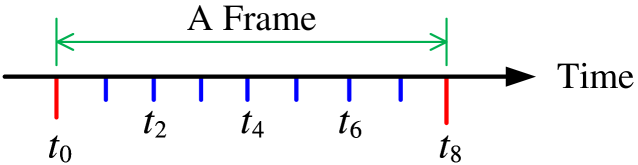
### Visual Description
\n
## Diagram: Temporal Frame Representation
### Overview
The image depicts a timeline representing a temporal frame, labeled "A Frame," with specific time points marked along it. The timeline extends from time t₀ to t₈, with the frame spanning from t₀ to t₈.
### Components/Axes
* **Axis:** A horizontal line labeled "Time" extending from left to right.
* **Time Points:** Marked with vertical lines and labels: t₀, t₂, t₄, t₆, t₈.
* **Frame:** A green, double-headed arrow labeled "A Frame" spanning the entire timeline from t₀ to t₈.
* **Markers:** Red vertical lines at t₀ and t₈, and blue vertical lines at t₂, t₄, and t₆.
### Detailed Analysis
The timeline is a linear representation of time. The frame "A Frame" encompasses the entire duration from t₀ to t₈. The time points are evenly spaced, suggesting a uniform time scale.
* **t₀:** Marked with a red vertical line.
* **t₂:** Marked with a blue vertical line.
* **t₄:** Marked with a blue vertical line.
* **t₆:** Marked with a blue vertical line.
* **t₈:** Marked with a red vertical line.
The distance between each time point (t₀ to t₂, t₂ to t₄, etc.) appears to be equal, indicating consistent time intervals.
### Key Observations
The diagram highlights the start and end points of the frame (t₀ and t₈) with red markers, while intermediate points within the frame (t₂, t₄, t₆) are marked with blue markers. This could indicate specific events or states occurring at these time points.
### Interpretation
This diagram likely represents a sequence of events or a process occurring within a defined time frame. The "A Frame" represents the total duration of the process. The red markers at t₀ and t₈ could signify the beginning and end of the process, or perhaps initial and final states. The blue markers at t₂, t₄, and t₆ could represent intermediate steps, measurements, or states within the process. The diagram is a simplified representation and doesn't provide specific details about the nature of the events or process, but it clearly defines the temporal boundaries and key time points. It is a conceptual illustration rather than a data-rich chart.
</details>
Figure 1: True data-generating distributions might be time-varying in a frame.
Let $\mathbb{P}_{0,\mathbf{x},\mathbf{s},i}$ denote the true data-generating distribution at time point $t_{i}$ where $i=1,2,\ldots,8$ . Specifically, we have $(\mathbf{x}_{i},\mathbf{s}_{i})\sim\mathbb{P}_{0,\mathbf{x},\mathbf{s},i}$ for every $i$ . Therefore, the pilot data set (i.e., the training data set) $\{(\bm{x}_{1},\bm{s}_{1}),(\bm{x}_{2},\bm{s}_{2}),(\bm{x}_{3},\bm{s}_{3}),(\bm {x}_{4},\bm{s}_{4})\}$ can be seen as realizations of the mean distribution $\mathbb{P}_{\text{train},0,\mathbf{x},\mathbf{s}}$ of underlying true training-data distributions where $\mathbb{P}_{\text{train},0,\mathbf{x},\mathbf{s}}=\sum^{4}_{i=1}h_{i}\mathbb{P }_{0,\mathbf{x},\mathbf{s},i}$ , which is a mixture distribution with mixing weights $0\leq h_{1},h_{2},h_{3},h_{4}\leq 1$ ; $\sum^{4}_{i=1}h_{i}=1$ . Similarly, the communication data set (i.e., the testing data set) $\{(\bm{x}_{5},\bm{s}_{5}),(\bm{x}_{6},\bm{s}_{6}),(\bm{x}_{7},\bm{s}_{7}),(\bm {x}_{8},\bm{s}_{8})\}$ can be seen as realizations of the mean $\mathbb{P}_{\text{test},0,\mathbf{x},\mathbf{s}}$ of the underlying true testing-data distributions where $\mathbb{P}_{\text{test},0,\mathbf{x},\mathbf{s}}=\sum^{8}_{i=5}h_{i}\mathbb{P} _{0,\mathbf{x},\mathbf{s},i}$ , with mixing weights $0\leq h_{5},h_{6},h_{7},h_{8}\leq 1$ ; $\sum^{8}_{i=5}h_{i}=1$ .
Suppose that
$$
d(\hat{\mathbb{P}}_{\text{train},\mathbf{x},\mathbf{s}},~{}\mathbb{P}_{\text{
train},0,\mathbf{x},\mathbf{s}})\leq\epsilon_{1},
$$
where $\hat{\mathbb{P}}_{\text{train},\mathbf{x},\mathbf{s}}\coloneqq\frac{1}{4}\sum^ {4}_{i=1}\delta_{(\bm{x}_{i},\bm{s}_{i})}$ is the data-driven estimate of $\mathbb{P}_{\text{train},0,\mathbf{x},\mathbf{s}}$ and
$$
d(\mathbb{P}_{\text{train},0,\mathbf{x},\mathbf{s}},~{}\mathbb{P}_{\text{test}
,0,\mathbf{x},\mathbf{s}})\leq\epsilon_{2},
$$
for some $\epsilon_{1},\epsilon_{2}\geq 0$ . We have the uncertainty quantification
$$
d(\mathbb{P}_{\text{test},0,\mathbf{x},\mathbf{s}},~{}\hat{\mathbb{P}}_{\text{
train},\mathbf{x},\mathbf{s}})\leq\epsilon\coloneqq\epsilon_{1}+\epsilon_{2}.
$$
Therefore, the distributionally robust modeling and solution framework is still valid to hedge against the distributional uncertainty in the nominal distribution $\hat{\mathbb{P}}_{\text{train},\mathbf{x},\mathbf{s}}$ compared to the underlying true distribution $\mathbb{P}_{\text{test},0,\mathbf{x},\mathbf{s}}$ . When $\mathbb{P}_{\text{train},0,\mathbf{x},\mathbf{s}}=\mathbb{P}_{\text{test},0, \mathbf{x},\mathbf{s}}$ , as assumed in the main body of the article, we have $\epsilon_{1}\to 0$ and $\epsilon\to\epsilon_{2}=0$ as the pilot size tends to infinity; however, when $\mathbb{P}_{\text{train},0,\mathbf{x},\mathbf{s}}\neq\mathbb{P}_{\text{test},0 ,\mathbf{x},\mathbf{s}}$ , the radius $\epsilon\to\epsilon_{2}\neq 0$ although $\epsilon_{1}\to 0$ .
Another justification for the DRO method is as follows. Suppose that there exists $\epsilon\geq 0$ such that
$$
d(\mathbb{P}_{0,\mathbf{x},\mathbf{s},i},~{}\hat{\mathbb{P}}_{\text{train},
\mathbf{x},\mathbf{s}})\leq\epsilon,~{}~{}~{}\forall i\in\{1,2,\ldots,8\}.
$$
It means that, at every snapshot in the frame, the true data-generating distribution is included in the uncertainty set. Hence, the DRO cost can still upper bound the true cost even though the true distribution is time-varying; cf. Fact 1.
## Appendix D Additional Discussions on Distributionally Robust Estimation
To develop this article, the typical minimum mean-squared error (MSE) criterion is employed; see (7) and (10). Accordingly, the distributionally robust receive combining framework in this article is exemplified using the MSE cost function. The cost function for wireless signal estimation, however, can be any Borel-measurable function $h:\mathbb{C}^{M}\times\mathbb{C}^{M}\to\mathbb{R}_{+}$ . As a result, the optimal estimation problem under the distribution $\mathbb{P}_{\mathbf{x},\mathbf{s}}$ is given by
$$
\min_{\bm{\phi}\in\mathcal{B}_{\mathbb{C}^{N}\to\mathbb{C}^{M}}}\mathbb{E}_{
\mathbf{x},\mathbf{s}}h[\bm{\phi}(\mathbf{x}),\mathbf{s}]. \tag{76}
$$
Specific examples of $h$ in wireless communications can be, e.g., mean absolute error, Huber’s cost function [37, 38] where $h$ is no longer quadratic as in (7) and (10). Accordingly, when the distributional uncertainty exists in $\mathbb{P}_{\mathbf{x},\mathbf{s}}$ , the distributionally robust receive combining framework becomes
$$
\min_{\bm{\phi}\in\mathcal{B}_{\mathbb{C}^{N}\to\mathbb{C}^{M}}}\max_{\mathbb{
P}_{\mathbf{x},\mathbf{s}}\in\mathcal{U}_{\mathbf{x},\mathbf{s}}}\mathbb{E}_{
\mathbf{x},\mathbf{s}}h[\bm{\phi}(\mathbf{x}),\mathbf{s}]. \tag{77}
$$
Problem (77) is generally challenging to solve because it is an infinite-dimensional program. Therefore, in practice, we can limit the feasible region of $\bm{\phi}$ to a parameterized subspace of $\mathcal{B}_{\mathbb{C}^{N}\to\mathbb{C}^{M}}$ , for example, a reproducing kernel Hilbert space $\mathcal{H}$ or a neural network function space $\mathcal{K}$ ; see Section II. Consequently, Problem (77) is approximated by the following finite-dimensional (in terms of $\bm{W}$ ) program
$$
\min_{\bm{W}}\max_{\mathbb{P}_{\mathbf{x},\mathbf{s}}\in\mathcal{U}_{\mathbf{x
},\mathbf{s}}}\mathbb{E}_{\mathbf{x},\mathbf{s}}h[\bm{\phi}_{\bm{W}}(\mathbf{x
}),\mathbf{s}], \tag{78}
$$
where $\bm{W}$ parameterizes $\bm{\phi}$ and lies in real or complex coordinate spaces; note that both $\mathcal{H}$ and $\mathcal{K}$ can be dense in $\mathcal{B}$ . Under the MSE cost function, (78) is particularized in (19) for linear function spaces, in (57) for reproducing kernel Hilbert spaces, and in (69) for neural network function spaces, which build this article in a technically tractable manner.
The distributionally robust receive combining problem (77) under generic cost functions $h$ and generic feasible regions of $\bm{\phi}$ can be technically challenging. Even for the simplified problem (78), the solution method can be quite complex, and closed-form solutions cannot be generally guaranteed; see, e.g., [39, 40]. The complication further arises when the distributional uncertainty sets $\mathcal{U}_{\mathbf{x},\mathbf{s}}$ for $\mathbb{P}_{\mathbf{x},\mathbf{s}}$ are complicated; see, e.g., [32]. Therefore, this article serves as the starting point of distributionally robust receive combining, in which closed-form solutions are largely ensured by leveraging
1. the MSE cost function as in (7) and (10);
1. the linear function spaces as in (19) and reproducing kernel Hilbert spaces as in (57);
1. the second-moment-based uncertainty sets in Definitions 1, 2, 3, and 4; see also Corollary 1, Claim 2, and Example 4.
Note that even under the features F1) and F2), the closed-form solutions cannot be guaranteed. For example, if Wasserstein or F-norm uncertainty sets are used, the associated distributionally robust receive combining problems can be computationally heavy; see (47) and (52) as well as Propositions 1 and 2. However, for emerging high-performance computing devices, the computational burden may be no longer an issue in the future. Hence, advanced distributionally robust receive combining formulations based on (77) and (78) are still attractive for future-generation communication systems. This article seeks to provide a foundation for this direction.
## Appendix E Proof of Lemma 1
* Proof:*
The objective function of Problem (19) equals to
$$
\left\langle\left[\begin{array}[]{cc}\bm{W}^{\mathsf{H}}\bm{W}&-\bm{W}^{
\mathsf{H}}\\
-\bm{W}&\bm{I}_{M}\end{array}\right],~{}\left[\begin{array}[]{cc}\bm{R}_{x}&
\bm{R}_{xs}\\
\bm{R}^{\mathsf{H}}_{xs}&\bm{R}_{s}\end{array}\right]\right\rangle, \tag{79}
$$
where $\langle\bm{A},\bm{B}\rangle\coloneqq\operatorname{Tr}\bm{A}^{\mathsf{H}}\bm{B}$ for two matrices $\bm{A}$ and $\bm{B}$ . Therefore, the objective function of (19) is convex in $\bm{W}$ and linear (thus concave) in the matrix variable $\bm{R}$ . Hence, due to Sion’s minimax theorem [41, Corollary 3.3], Problem (19) is equivalent to
$$
\begin{array}[]{cl}\displaystyle\max_{\bm{R}}\min_{\bm{W}}&\operatorname{Tr}
\big{[}\bm{W}\bm{R}_{x}\bm{W}^{\mathsf{H}}-\bm{W}\bm{R}_{xs}-\bm{R}^{\mathsf{H
}}_{xs}\bm{W}^{\mathsf{H}}+\bm{R}_{s}\big{]}\\
\text{s.t.}&d_{0}(\bm{R},~{}\hat{\bm{R}})\leq\epsilon_{0},\\
&\bm{R}\succeq\bm{0}.\end{array} \tag{80}
$$
Note that the feasible region of $\bm{R}$ is compact convex, and that of $\bm{W}$ (i.e., $\mathbb{C}^{M\times N}$ ) is convex. For every given $\bm{R}$ , the inner minimization sub-problem of (80) is solved by the Wiener beamformer $\bm{W}^{\star}_{\text{Wiener}}=\bm{R}^{\mathsf{H}}_{xs}\bm{R}^{-1}_{x}$ , which transforms (80) to (21). This completes the proof. $\square$ ∎
## Appendix F Proof of Theorem 1
* Proof:*
Consider the following optimization problem
$$
\begin{array}[]{cl}\displaystyle\max_{\bm{R}}&\operatorname{Tr}\big{[}-\bm{R}^
{\mathsf{H}}_{xs}\bm{R}^{-1}_{x}\bm{R}_{xs}+\bm{R}_{s}\big{]}\\
\text{s.t.}&\bm{R}\succeq\bm{R}_{2},\\
&\bm{R}_{x}\succ\bm{0},\end{array} \tag{81}
$$
which, due to Lemma 1, is equivalent [in the sense of the same optimal objective value and maximizer(s) $\bm{R}^{\star}$ ] to
$$
\begin{array}[]{cl}\displaystyle\min_{\bm{W}}\max_{\bm{R}}&\left\langle\left[
\begin{array}[]{cc}\bm{W}^{\mathsf{H}}\bm{W}&-\bm{W}^{\mathsf{H}}\\
-\bm{W}&\bm{I}_{M}\end{array}\right],~{}\left[\begin{array}[]{cc}\bm{R}_{x}&
\bm{R}_{xs}\\
\bm{R}^{\mathsf{H}}_{xs}&\bm{R}_{s}\end{array}\right]\right\rangle\\
\text{s.t.}&\bm{R}\succeq\bm{R}_{2},\\
&\bm{R}_{x}\succ\bm{0}.\end{array} \tag{82}
$$
Note that $\left[\begin{array}[]{cc}\bm{W}^{\mathsf{H}}\bm{W}&-\bm{W}^{\mathsf{H}}\\ -\bm{W}&\bm{I}_{M}\end{array}\right]\succeq\bm{0},$ because for all $\bm{x}\in\mathbb{C}^{N}$ and $\bm{y}\in\mathbb{C}^{M}$ , we have
$$
[\bm{x}^{\mathsf{H}},~{}\bm{y}^{\mathsf{H}}]\left[\begin{array}[]{cc}\bm{W}^{
\mathsf{H}}\bm{W}&-\bm{W}^{\mathsf{H}}\\
-\bm{W}&\bm{I}_{M}\end{array}\right]\left[\begin{array}[]{c}\bm{x}\\
\bm{y}\end{array}\right]=\|\bm{W}\bm{x}-\bm{y}\|^{2}_{2}\geq 0.
$$
Therefore, for every given $\bm{W}$ , the objective function of (82) is increasing in $\bm{R}$ . As a result, the objective value of (81) is lower-bounded at $\bm{R}_{2}$ : To be specific, $\forall\bm{R}\succeq\bm{R}_{2}$ , we have
$$
\operatorname{Tr}\big{[}-\bm{R}^{\mathsf{H}}_{xs}\bm{R}^{-1}_{x}\bm{R}_{xs}+
\bm{R}_{s}\big{]}\\
\geq\operatorname{Tr}\big{[}-\bm{R}^{\mathsf{H}}_{2,xs}\bm{R}^{-1}_{2,x}\bm{R}
_{2,xs}+\bm{R}_{2,s}\big{]},
$$
i.e., $f_{1}(\bm{R})\geq f_{1}(\bm{R}_{2})$ , which proves the first part. On the other hand, if $\bm{R}_{1,x}\succeq\bm{R}_{2,x}\succ\bm{0}$ , we have $\bm{R}^{-1}_{2,x}\succeq\bm{R}^{-1}_{1,x}$ . As a result, $f_{2}(\bm{R}_{1,x})-f_{2}(\bm{R}_{2,x})=\operatorname{Tr}\left[{\bm{R}^{ \mathsf{H}}_{xs}(\bm{R}^{-1}_{2,x}-\bm{R}^{-1}_{1,x})\bm{R}_{xs}}\right]\geq 0$ , completing the proof. $\square$ ∎
## Appendix G Proof of Proposition 3
* Proof:*
Letting $\underline{\mathbf{z}}\coloneqq\bm{\varphi}(\underline{\mathbf{x}})$ , (57) can be rewritten as
$$
\min_{\bm{W}\in\mathbb{R}^{2M\times L}}\max_{\mathbb{P}_{\underline{\mathbf{z}
},\underline{\mathbf{s}}}\in\mathcal{U}_{\underline{\mathbf{z}},\underline{
\mathbf{s}}}}\operatorname{Tr}\mathbb{E}_{\underline{\mathbf{z}},\underline{
\mathbf{s}}}[\bm{W}\underline{\mathbf{z}}-\underline{\mathbf{s}}][\bm{W}
\underline{\mathbf{z}}-\underline{\mathbf{s}}]^{\mathsf{T}}. \tag{83}
$$
Tantamount to the distributionally robust beamforming problem (19), Problem (83) reduces to (58) where
$$
\hat{\bm{R}}_{\underline{z}}\coloneqq\frac{1}{L}\sum^{L}_{i=1}\underline{\bm{z
}}_{i}\underline{\bm{z}}^{\mathsf{T}}_{i}=\frac{1}{L}\sum^{L}_{i=1}\bm{\varphi
}(\underline{\bm{x}}_{i})\bm{\varphi}^{\mathsf{T}}(\underline{\bm{x}}_{i})=
\frac{1}{L}\bm{K}^{2},
$$
$$
\hat{\bm{R}}_{\underline{zs}}\coloneqq\frac{1}{L}\sum^{L}_{i=1}\underline{\bm{
z}}_{i}\underline{\bm{s}}^{\mathsf{T}}_{i}=\frac{1}{L}\sum^{L}_{i=1}\bm{
\varphi}(\underline{\bm{x}}_{i})\cdot\underline{\bm{s}}^{\mathsf{T}}_{i}=\frac
{1}{L}\bm{K}\underline{\bm{S}}^{\mathsf{T}},
$$
$$
\hat{\bm{R}}_{\underline{s}}\coloneqq\frac{1}{L}\sum^{L}_{i=1}\underline{\bm{s
}}_{i}\underline{\bm{s}}^{\mathsf{T}}_{i}=\frac{1}{L}\sum^{L}_{i=1}\underline{
\bm{s}}_{i}\cdot\underline{\bm{s}}^{\mathsf{T}}_{i}=\frac{1}{L}\underline{\bm{
S}}\underline{\bm{S}}^{\mathsf{T}},
$$
and
$$
\bm{K}\coloneqq[\bm{\varphi}(\underline{\bm{x}}_{1}),\bm{\varphi}(\underline{
\bm{x}}_{2}),\ldots,\bm{\varphi}(\underline{\bm{x}}_{L})]\in\mathbb{R}^{L
\times L}.
$$
The rest claims are due to Lemma 1; NB: $\bm{K}$ is invertible. $\square$ ∎
## References
- [1] T. Lo, H. Leung, and J. Litva, “Nonlinear beamforming,” Electronics Letters, vol. 4, no. 27, pp. 350–352, 1991.
- [2] S. Yang and L. Hanzo, “Fifty years of MIMO detection: The road to large-scale MIMOs,” IEEE Commun. Surveys Tuts., vol. 17, no. 4, pp. 1941–1988, 2015.
- [3] A. M. Elbir, K. V. Mishra, S. A. Vorobyov, and R. W. Heath, “Twenty-five years of advances in beamforming: From convex and nonconvex optimization to learning techniques,” IEEE Signal Processing Mag., vol. 40, no. 4, pp. 118–131, 2023.
- [4] S. Chen, S. Tan, L. Xu, and L. Hanzo, “Adaptive minimum error-rate filtering design: A review,” Signal Processing, vol. 88, no. 7, pp. 1671–1697, 2008.
- [5] S. Chen, A. Wolfgang, C. J. Harris, and L. Hanzo, “Symmetric RBF classifier for nonlinear detection in multiple-antenna-aided systems,” IEEE Trans. Neural Networks, vol. 19, no. 5, pp. 737–745, 2008.
- [6] A. Navia-Vazquez, M. Martinez-Ramon, L. E. Garcia-Munoz, and C. G. Christodoulou, “Approximate kernel orthogonalization for antenna array processing,” IEEE Trans. Antennas Propagat., vol. 58, no. 12, pp. 3942–3950, 2010.
- [7] M. Neinavaie, M. Derakhtian, and S. A. Vorobyov, “Lossless dimension reduction for integer least squares with application to sphere decoding,” IEEE Trans. Signal Processing, vol. 68, pp. 6547–6561, 2020.
- [8] J. Liao, J. Zhao, F. Gao, and G. Y. Li, “Deep learning aided low complex breadth-first tree search for MIMO detection,” IEEE Trans. Wireless Commun., 2023.
- [9] D. A. Awan, R. L. Cavalcante, M. Yukawa, and S. Stanczak, “Robust online multiuser detection: A hybrid model-data driven approach,” IEEE Trans. Signal Processing, 2023.
- [10] H. Ye, G. Y. Li, and B.-H. Juang, “Power of deep learning for channel estimation and signal detection in OFDM systems,” IEEE Wireless Commun. Lett., vol. 7, no. 1, pp. 114–117, 2017.
- [11] H. He, C.-K. Wen, S. Jin, and G. Y. Li, “Model-driven deep learning for MIMO detection,” IEEE Trans. Signal Processing, vol. 68, pp. 1702–1715, 2020.
- [12] N. Van Huynh and G. Y. Li, “Transfer learning for signal detection in wireless networks,” IEEE Wireless Commun. Lett., vol. 11, no. 11, pp. 2325–2329, 2022.
- [13] J. Li, P. Stoica, and Z. Wang, “On robust Capon beamforming and diagonal loading,” IEEE Trans. Signal Processing, vol. 51, no. 7, pp. 1702–1715, 2003.
- [14] R. G. Lorenz and S. P. Boyd, “Robust minimum variance beamforming,” IEEE Trans. Signal Processing, vol. 53, no. 5, pp. 1684–1696, 2005.
- [15] X. Zhang, Y. Li, N. Ge, and J. Lu, “Robust minimum variance beamforming under distributional uncertainty,” in 2015 IEEE International Conference on Acoustics, Speech and Signal Processing (ICASSP). IEEE, 2015, pp. 2514–2518.
- [16] B. Li, Y. Rong, J. Sun, and K. L. Teo, “A distributionally robust minimum variance beamformer design,” IEEE Signal Processing Lett., vol. 25, no. 1, pp. 105–109, 2017.
- [17] Y. Huang, W. Yang, and S. A. Vorobyov, “Robust adaptive beamforming maximizing the worst-case SINR over distributional uncertainty sets for random inc matrix and signal steering vector,” in ICASSP 2022-2022 IEEE International Conference on Acoustics, Speech and Signal Processing (ICASSP). IEEE, 2022, pp. 4918–4922.
- [18] Y. Huang, H. Fu, S. A. Vorobyov, and Z.-Q. Luo, “Robust adaptive beamforming via worst-case SINR maximization with nonconvex uncertainty sets,” IEEE Trans. Signal Processing, vol. 71, pp. 218–232, 2023.
- [19] H. Cox, R. Zeskind, and M. Owen, “Robust adaptive beamforming,” IEEE Trans. Acoust., Speech, Signal Processing, vol. 35, no. 10, pp. 1365–1376, 1987.
- [20] K. Harmanci, J. Tabrikian, and J. L. Krolik, “Relationships between adaptive minimum variance beamforming and optimal source localization,” IEEE Trans. Signal Processing, vol. 48, no. 1, pp. 1–12, 2000.
- [21] F. Liu, L. Zhou, C. Masouros, A. Li, W. Luo, and A. Petropulu, “Toward dual-functional radar-communication systems: Optimal waveform design,” IEEE Trans. Signal Processing, vol. 66, no. 16, pp. 4264–4279, 2018.
- [22] J. A. Zhang, F. Liu, C. Masouros, R. W. Heath, Z. Feng, L. Zheng, and A. Petropulu, “An overview of signal processing techniques for joint communication and radar sensing,” IEEE J. Select. Topics Signal Processing, vol. 15, no. 6, pp. 1295–1315, 2021.
- [23] Y. Xiong, F. Liu, Y. Cui, W. Yuan, T. X. Han, and G. Caire, “On the fundamental tradeoff of integrated sensing and communications under Gaussian channels,” IEEE Trans. Inform. Theory, 2023.
- [24] K. P. Murphy, Machine Learning: A Probabilistic Perspective. MIT Press, 2012.
- [25] C. M. Bishop and N. M. Nasrabadi, Pattern Recognition and Machine Learning. Springer, 2006, vol. 4, no. 4.
- [26] G. Li and J. Ding, “Towards understanding variation-constrained deep neural networks,” IEEE Trans. Signal Processing, vol. 71, pp. 631–640, 2023.
- [27] S. Shafieezadeh-Abadeh, D. Kuhn, and P. M. Esfahani, “Regularization via mass transportation,” Journal of Machine Learning Research, vol. 20, no. 103, pp. 1–68, 2019.
- [28] M. Staib and S. Jegelka, “Distributionally robust optimization and generalization in kernel methods,” Advances in Neural Information Processing Systems, vol. 32, 2019.
- [29] E. Delage and Y. Ye, “Distributionally robust optimization under moment uncertainty with application to data-driven problems,” Operations Research, vol. 58, no. 3, pp. 595–612, 2010.
- [30] S. Wang, “Distributionally robust state estimation for jump linear systems,” IEEE Trans. Signal Processing, 2023.
- [31] J. Li, S. Lin, J. Blanchet, and V. A. Nguyen, “Tikhonov regularization is optimal transport robust under martingale constraints,” Advances in Neural Information Processing Systems, vol. 35, pp. 17 677–17 689, 2022.
- [32] D. Kuhn, P. M. Esfahani, V. A. Nguyen, and S. Shafieezadeh-Abadeh, “Wasserstein distributionally robust optimization: Theory and applications in machine learning,” in Operations Research & Management Science in the Age of Analytics. Informs, 2019, pp. 130–166.
- [33] J. Blanchet, Y. Kang, and K. Murthy, “Robust Wasserstein profile inference and applications to machine learning,” Journal of Applied Probability, vol. 56, no. 3, pp. 830–857, 2019.
- [34] C. Shorten and T. M. Khoshgoftaar, “A survey on image data augmentation for deep learning,” Journal of Big Data, vol. 6, 2019.
- [35] G. Saon, Z. Tüske, K. Audhkhasi, and B. Kingsbury, “Sequence noise injected training for end-to-end speech recognition,” in ICASSP 2019-2019 IEEE International Conference on Acoustics, Speech and Signal Processing (ICASSP). IEEE, 2019, pp. 6261–6265.
- [36] K. Vu, J. C. Snyder, L. Li, M. Rupp, B. F. Chen, T. Khelif, K.-R. Müller, and K. Burke, “Understanding kernel ridge regression: Common behaviors from simple functions to density functionals,” International Journal of Quantum Chemistry, vol. 115, no. 16, pp. 1115–1128, 2015.
- [37] X. Wang and H. V. Poor, “Robust adaptive array for wireless communications,” IEEE J. Select. Areas in Commun., vol. 16, no. 8, pp. 1352–1366, 1998.
- [38] V. Katkovnik, M.-S. Lee, and Y.-H. Kim, “Performance study of the minimax robust phased array for wireless communications,” IEEE Trans. Wireless Commun., vol. 54, no. 4, pp. 608–613, 2006.
- [39] H. Rahimian and S. Mehrotra, “Frameworks and results in distributionally robust optimization,” Open Journal of Mathematical Optimization, vol. 3, pp. 1–85, 2022.
- [40] D. Kuhn, S. Shafiee, and W. Wiesemann, “Distributionally robust optimization,” Acta Numerica, 2024.
- [41] M. Sion, “On general minimax theorems.” Pacific Journal of Mathematics, vol. 8, no. 1, pp. 171 – 176, 1958.
|
<details>
<summary>x2.png Details</summary>
### Visual Description
\n
## Photograph: Portrait of a Man
### Overview
The image is a head-and-shoulders portrait of a man against a plain white background. The subject is facing forward, looking directly at the camera. The lighting is even, and the focus is sharp on the face.
### Components/Axes
There are no axes or components in the traditional sense of a chart or diagram. The image consists of the following visible elements:
* **Subject:** A man with short, dark hair.
* **Clothing:** A blue t-shirt with the word "PERFECT" printed in white, lowercase letters across the chest.
* **Background:** A solid white background.
### Detailed Analysis or Content Details
The man appears to be of East Asian descent. He has dark eyebrows, dark eyes, and a neutral expression. His skin tone is fair. The t-shirt is a muted blue color. The word "PERFECT" is printed in a simple, sans-serif font. The image is well-lit, with minimal shadows.
### Key Observations
The image is a straightforward portrait, likely intended for identification purposes (e.g., a passport photo, employee ID). The subject's neutral expression and direct gaze contribute to a formal and professional appearance. The word "PERFECT" on the t-shirt is a potentially interesting detail, though its significance is unclear without further context.
### Interpretation
The image provides no quantitative data or trends. It is a visual representation of an individual. The choice of a plain background and direct gaze suggests a desire for clear and unambiguous identification. The inclusion of the word "PERFECT" on the t-shirt could be a personal statement, a brand affiliation, or simply a coincidental element of the subject's attire. Without additional information, it is difficult to draw further conclusions. The image is primarily descriptive and lacks inherent analytical depth.
</details>
| Shixiong Wang (Member, IEEE) received the B.Eng. degree in detection, guidance, and control technology, and the M.Eng. degree in systems and control engineering from the School of Electronics and Information, Northwestern Polytechnical University, China, in 2016 and 2018, respectively. He received his Ph.D. degree from the Department of Industrial Systems Engineering and Management, National University of Singapore, Singapore, in 2022. He is currently a Postdoctoral Research Associate with the Intelligent Transmission and Processing Laboratory, Imperial College London, London, United Kingdom, from May 2023. He was a Postdoctoral Research Fellow with the Institute of Data Science, National University of Singapore, Singapore, from March 2022 to March 2023. His research interest includes statistics and optimization theories with applications in signal processing (especially optimal estimation theory), machine learning (especially generalization error theory), and control technology. |
| --- | --- |
|
<details>
<summary>extracted/6550238/Figures/dw.jpg Details</summary>
### Visual Description
\n
## Photograph: Portrait of a Man
### Overview
The image is a headshot portrait of a man against a dark blue background. The image appears to be a professional photograph, likely a headshot for business or official purposes. There is no data or chart information present.
### Components/Axes
There are no axes, legends, or scales present in this image. It is a photograph of a person.
### Detailed Analysis or Content Details
The subject is a man of East Asian descent, appearing to be in his late 20s to early 40s. He has short, dark hair, dark eyes, and a fair complexion. He is wearing a white collared shirt with a subtle checkered pattern. The lighting is soft and even, illuminating his face and upper torso. The background is a solid, dark blue color, providing contrast and focusing attention on the subject. The image is well-composed, with the subject centered in the frame.
### Key Observations
The image is a straightforward portrait with no apparent anomalies or unusual features. The subject's expression is neutral and professional.
### Interpretation
The image serves as a visual representation of an individual. Without additional context, it's difficult to determine the purpose of the photograph beyond identification. It is likely intended to convey a sense of professionalism and trustworthiness. The lack of any surrounding information or data suggests the image is meant to stand alone as a representation of the person depicted. There is no data to analyze beyond the visual characteristics of the subject and the photographic composition.
</details>
| Wei Dai (Member, IEEE) received the Ph.D. degree from the University of Colorado Boulder, Boulder, Colorado, in 2007. He is currently a Senior Lecturer (Associate Professor) in the Department of Electrical and Electronic Engineering, Imperial College London, London, UK. From 2007 to 2011, he was a Postdoctoral Research Associate with the University of Illinois Urbana-Champaign, Champaign, IL, USA. His research interests include electromagnetic sensing, biomedical imaging, wireless communications, and information theory. |
| --- | --- |
|
<details>
<summary>extracted/6550238/Figures/LiG_Photo24.jpg Details</summary>
### Visual Description
\n
## Photograph: Portrait of a Man
### Overview
The image is a head-and-shoulders portrait of an East Asian man, likely taken for professional or official purposes. The background is a plain white, creating a high-contrast image focused on the subject. The image does not contain charts, diagrams, or data tables. It is a photograph of a person.
### Components/Axes
There are no axes, legends, or scales present in this image. The primary component is the subject's face and upper body. The subject is wearing a dark suit jacket, a white shirt, and a patterned blue tie.
### Detailed Analysis or Content Details
The man appears to be approximately 60-75 years old, with graying hair. He has a fair complexion with visible age spots. His expression is neutral, looking directly at the camera. He is wearing glasses. The lighting is even, illuminating his face without harsh shadows. The suit jacket is dark, possibly navy or black. The tie has a repeating pattern of small white shapes on a blue background. The shirt is a standard white dress shirt with a visible collar.
### Key Observations
The image is a formal portrait, suggesting the subject holds a position of authority or is being presented in a professional context. The neutral expression and direct gaze convey a sense of seriousness and composure. The high-quality lighting and composition indicate a professional photographer was likely used.
### Interpretation
The photograph likely serves as an official portrait for identification or representation. The subject's attire and demeanor suggest a professional or leadership role. The image is designed to convey trustworthiness and competence. There is no data or quantifiable information present; the image relies on visual cues to communicate information about the subject's character and status. The image is a representation of a person, and its meaning is derived from cultural conventions associated with portraiture and professional imagery. Without additional context, it is difficult to determine the specific purpose or significance of the portrait.
</details>
| Geoffrey Ye Li is currently a Chair Professor at Imperial College London, UK. Before joining Imperial in 2020, he was a Professor at Georgia Institute of Technology for 20 years and a Principal Technical Staff Member with AT&T Labs – Research (previous Bell Labs) for five years. He made fundamental contributions to orthogonal frequency division multiplexing (OFDM) for wireless communications, established a framework on resource cooperation in wireless networks, and introduced deep learning to communications. In these areas, he has published over 700 journal and conference papers in addition to over 40 granted patents. His publications have been cited around 80,000 times with an H-index over 130. He has been listed as a Highly Cited Researcher by Clarivate/Web of Science almost every year. Dr. Geoffrey Ye Li was elected to Fellow of the Royal Academic of Engineering (FREng), IEEE Fellow, and IET Fellow for his contributions to signal processing for wireless communications. He received 2024 IEEE Eric E. Sumner Award, 2019 IEEE ComSoc Edwin Howard Armstrong Achievement Award, and several other awards from IEEE Signal Processing, Vehicular Technology, and Communications Societies. |
| --- | --- |
Supplementary Materials
## Appendix H Additional Experimental Results
Complementary to experimental setups in Section VI, we consider pure complex Gaussian channel noises. First, we suppose that the transmit antennas emit continuous-valued complex signals; without loss of generality, Gaussian signals are used in experiments. The performance evaluation measure is therefore the mean-squared error (MSE). The experimental results are shown in Fig. 2.
<details>
<summary>x3.png Details</summary>

### Visual Description
\n
## Line Chart: MSE vs. Pilot Size for Different Signal Processing Techniques
### Overview
This line chart depicts the Mean Squared Error (MSE) as a function of Pilot Size for five different signal processing techniques: Capon, Kernel, Wiener, Wiener-CE, and Zero-Forcing (ZF). The chart aims to compare the performance of these techniques in terms of error reduction as the pilot size increases.
### Components/Axes
* **X-axis:** Pilot Size, ranging from approximately 0 to 80.
* **Y-axis:** MSE (Mean Squared Error), ranging from approximately 0 to 1.
* **Legend:** Located in the top-right corner, identifying each line with a unique color:
* Capon (Green)
* Kernel (Light Blue)
* Wiener (Red)
* Wiener-CE (Dark Blue, dashed)
* ZF (Magenta)
### Detailed Analysis
Here's a breakdown of each line's trend and approximate data points:
* **Capon (Green):** The line starts at approximately MSE = 0.95 at Pilot Size = 0. It initially decreases rapidly to around MSE = 0.8 at Pilot Size = 10, then fluctuates between approximately 0.75 and 0.95 for the remainder of the range, showing no clear trend.
* **Kernel (Light Blue):** The line begins at approximately MSE = 0.85 at Pilot Size = 0. It decreases steadily to around MSE = 0.6 at Pilot Size = 80, exhibiting a slow, downward trend.
* **Wiener (Red):** This line shows the most significant decrease. It starts at approximately MSE = 0.8 at Pilot Size = 0 and rapidly drops to around MSE = 0.25 at Pilot Size = 40. It continues to decrease, reaching approximately MSE = 0.2 at Pilot Size = 80.
* **Wiener-CE (Dark Blue, dashed):** The line starts at approximately MSE = 0.65 at Pilot Size = 0. It decreases to around MSE = 0.2 at Pilot Size = 20 and remains relatively stable, fluctuating between approximately 0.18 and 0.25 for the rest of the range.
* **ZF (Magenta):** The line begins at approximately MSE = 0.6 at Pilot Size = 0. It initially decreases to around MSE = 0.7 at Pilot Size = 10, then fluctuates between approximately 0.7 and 0.9 for the remainder of the range, showing no clear trend.
### Key Observations
* The Wiener filter demonstrates the most substantial reduction in MSE as Pilot Size increases.
* The Wiener-CE filter achieves a low MSE and maintains it with increasing Pilot Size.
* Capon and ZF exhibit high and fluctuating MSE values, indicating poor performance across the tested Pilot Size range.
* The Kernel filter shows a gradual decrease in MSE, but its performance is significantly worse than the Wiener filters.
* There is a clear divergence in performance between the Wiener-based methods and the other techniques.
### Interpretation
The data suggests that the Wiener filter is the most effective signal processing technique among those tested for minimizing MSE as Pilot Size increases. The Wiener-CE filter also performs well, achieving a low MSE and maintaining stability. The Capon and ZF techniques appear to be less effective, with consistently higher MSE values. The Kernel filter offers some improvement with increasing Pilot Size, but its performance is considerably lower than the Wiener filters.
The rapid decrease in MSE for the Wiener filter indicates that increasing the Pilot Size provides a significant benefit in reducing error. The stabilization of the Wiener-CE filter suggests that there is a point of diminishing returns, where further increases in Pilot Size do not lead to substantial improvements in performance. The fluctuating MSE values for Capon and ZF may indicate instability or sensitivity to noise.
This data could be used to inform the selection of an appropriate signal processing technique based on the desired level of accuracy and the available Pilot Size. The results highlight the importance of considering the trade-offs between performance, complexity, and computational cost when choosing a signal processing method.
</details>
(a) $N$ =8, SNR 10dB, $\bm{R}_{v}$ Estimated
<details>
<summary>x4.png Details</summary>
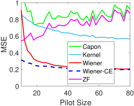
### Visual Description
\n
## Line Chart: MSE vs. Pilot Size for Different Algorithms
### Overview
This image presents a line chart comparing the Mean Squared Error (MSE) performance of five different algorithms (Capon, Kernel, Wiener, Wiener-CE, and ZF) as a function of Pilot Size. The chart visually demonstrates how the MSE changes for each algorithm as the pilot size increases from approximately 0 to 80.
### Components/Axes
* **X-axis:** "Pilot Size" ranging from 0 to 80, with tick marks at intervals of 10.
* **Y-axis:** "MSE" ranging from 0 to 1, with tick marks at intervals of 0.2.
* **Data Series:** Five distinct lines, each representing a different algorithm:
* Capon (Green solid line)
* Kernel (Light Blue solid line)
* Wiener (Red solid line)
* Wiener-CE (Dark Blue dashed line)
* ZF (Magenta solid line)
* **Legend:** Located in the top-right corner of the chart, associating each color with its corresponding algorithm.
### Detailed Analysis
Here's a breakdown of each algorithm's performance based on the chart:
* **Capon (Green):** The line fluctuates significantly, starting at approximately 0.95 at Pilot Size 0, oscillating between roughly 0.75 and 0.95 throughout the range, and ending around 0.9 at Pilot Size 80.
* **Kernel (Light Blue):** The line starts at approximately 0.85 at Pilot Size 0 and decreases to around 0.65 by Pilot Size 80, exhibiting a generally decreasing trend with some fluctuations.
* **Wiener (Red):** The line shows a steep decrease from approximately 0.9 at Pilot Size 0 to around 0.25 at Pilot Size 20. It then plateaus, remaining around 0.2 to 0.25 for the rest of the range, ending at approximately 0.22 at Pilot Size 80.
* **Wiener-CE (Dark Blue):** The line starts at approximately 0.3 at Pilot Size 0 and decreases rapidly to around 0.18 at Pilot Size 20. It then plateaus, remaining around 0.17 to 0.2 for the rest of the range, ending at approximately 0.19 at Pilot Size 80.
* **ZF (Magenta):** The line starts at approximately 0.65 at Pilot Size 0, decreases to around 0.75 at Pilot Size 10, then decreases to approximately 0.55 by Pilot Size 80, exhibiting a generally decreasing trend with some fluctuations.
### Key Observations
* The Wiener and Wiener-CE algorithms achieve the lowest MSE values across the entire range of Pilot Sizes.
* The Capon algorithm exhibits the highest and most volatile MSE values.
* The Kernel and ZF algorithms show moderate MSE values, with a decreasing trend as Pilot Size increases.
* All algorithms demonstrate a significant decrease in MSE as Pilot Size increases from 0 to 20, indicating that increasing the pilot size generally improves performance.
* After Pilot Size 20, the improvement in MSE diminishes for the Wiener and Wiener-CE algorithms, suggesting a point of diminishing returns.
### Interpretation
The chart suggests that the Wiener and Wiener-CE algorithms are the most effective in minimizing MSE for this particular application, especially as the pilot size increases. The Capon algorithm appears to be the least effective, with consistently high MSE values. The performance improvement observed with increasing pilot size indicates that providing more training data (represented by the pilot size) enhances the accuracy of the algorithms. The plateauing of the Wiener and Wiener-CE algorithms after Pilot Size 20 suggests that there is a limit to the benefits of increasing the pilot size beyond a certain point. This could be due to factors such as noise or the inherent limitations of the algorithms themselves. The differences in performance between the algorithms likely stem from their underlying assumptions and methodologies for estimating the signal or reducing noise. The chart provides valuable insights for selecting the most appropriate algorithm and determining the optimal pilot size for a given application.
</details>
(b) $N$ =8, SNR 10dB, $\bm{R}_{v}$ Known
<details>
<summary>x5.png Details</summary>
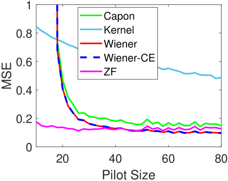
### Visual Description
\n
## Line Chart: MSE vs. Pilot Size for Different Algorithms
### Overview
This image presents a line chart illustrating the relationship between Mean Squared Error (MSE) and Pilot Size for five different algorithms: Capon, Kernel, Wiener, Wiener-CE, and Zero-Forcing (ZF). The chart aims to compare the performance of these algorithms in terms of error reduction as the pilot size increases.
### Components/Axes
* **X-axis:** Pilot Size, ranging from approximately 0 to 80. The axis is labeled "Pilot Size".
* **Y-axis:** Mean Squared Error (MSE), ranging from 0 to 1. The axis is labeled "MSE".
* **Legend:** Located in the top-right corner of the chart. It identifies each line with a corresponding color:
* Capon (Green)
* Kernel (Light Blue)
* Wiener (Red)
* Wiener-CE (Dark Blue, dashed)
* ZF (Magenta)
### Detailed Analysis
The chart displays five distinct lines, each representing the MSE values for a specific algorithm across varying pilot sizes.
* **Capon (Green):** The line starts at approximately MSE = 0.22 at Pilot Size = 0, decreases to approximately MSE = 0.16 at Pilot Size = 20, and then plateaus around MSE = 0.16-0.18 for Pilot Sizes between 20 and 80.
* **Kernel (Light Blue):** This line exhibits a significant drop in MSE from approximately MSE = 0.85 at Pilot Size = 0 to approximately MSE = 0.55 at Pilot Size = 20. It then continues to decrease, but at a slower rate, reaching approximately MSE = 0.5 at Pilot Size = 80.
* **Wiener (Red):** The line begins at approximately MSE = 0.22 at Pilot Size = 0, rapidly decreases to approximately MSE = 0.12 at Pilot Size = 20, and then stabilizes around MSE = 0.12-0.14 for Pilot Sizes between 20 and 80.
* **Wiener-CE (Dark Blue, dashed):** This line starts at approximately MSE = 0.22 at Pilot Size = 0, decreases to approximately MSE = 0.13 at Pilot Size = 20, and then remains relatively constant around MSE = 0.13-0.15 for Pilot Sizes between 20 and 80.
* **ZF (Magenta):** The line starts at approximately MSE = 0.18 at Pilot Size = 0, decreases slightly to approximately MSE = 0.16 at Pilot Size = 20, and then remains relatively constant around MSE = 0.16-0.18 for Pilot Sizes between 20 and 80.
### Key Observations
* The Kernel algorithm initially exhibits the highest MSE, but shows a consistent decrease as the pilot size increases.
* The Wiener and Wiener-CE algorithms demonstrate the lowest MSE values, particularly at larger pilot sizes.
* The Capon and ZF algorithms show relatively stable MSE values across the entire range of pilot sizes.
* All algorithms show a significant reduction in MSE as the pilot size increases from 0 to 20. Beyond Pilot Size = 20, the rate of MSE reduction diminishes for all algorithms.
### Interpretation
The data suggests that increasing the pilot size generally leads to a reduction in MSE for all the tested algorithms. However, the extent of this reduction varies significantly depending on the algorithm used. The Wiener and Wiener-CE algorithms consistently outperform the others in terms of minimizing MSE, especially at larger pilot sizes. The Kernel algorithm, while starting with a high MSE, shows a substantial improvement with increasing pilot size. The Capon and ZF algorithms provide relatively stable performance, but their MSE values are generally higher than those of the Wiener-based algorithms.
The rapid decrease in MSE from Pilot Size = 0 to Pilot Size = 20 indicates that the initial increase in pilot size has the most significant impact on error reduction. Beyond this point, the benefits of increasing the pilot size become less pronounced. This suggests that there may be a diminishing return on investment in terms of pilot size beyond a certain threshold. The differences in performance between the algorithms likely stem from their underlying assumptions and methodologies for signal estimation and interference cancellation.
</details>
(c) $N$ =16, SNR 10dB, $\bm{R}_{v}$ Estimated
<details>
<summary>x6.png Details</summary>
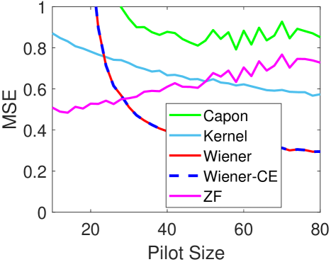
### Visual Description
\n
## Line Chart: MSE vs. Pilot Size for Different Algorithms
### Overview
The image presents a line chart illustrating the Mean Squared Error (MSE) as a function of Pilot Size for five different algorithms: Capon, Kernel, Wiener, Wiener-CE, and Zero-Forcing (ZF). The chart aims to compare the performance of these algorithms in terms of MSE as the pilot size varies.
### Components/Axes
* **X-axis:** Pilot Size, ranging from approximately 0 to 80.
* **Y-axis:** MSE (Mean Squared Error), ranging from 0 to 1.
* **Data Series:**
* Capon (Green solid line)
* Kernel (Light Blue solid line)
* Wiener (Red solid line)
* Wiener-CE (Dark Blue dashed line)
* ZF (Magenta solid line)
* **Legend:** Located in the top-right corner of the chart, associating colors with algorithm names.
### Detailed Analysis
Here's a breakdown of each data series and their trends:
* **Capon (Green):** The line starts at approximately 0.9 at a Pilot Size of 0, fluctuates around 0.8-0.9 until approximately Pilot Size 40, then decreases to around 0.75 before increasing again to approximately 0.9 at Pilot Size 80.
* **Kernel (Light Blue):** The line begins at approximately 0.85 at Pilot Size 0, and steadily decreases to approximately 0.6 at Pilot Size 80. The trend is generally downward, but with some fluctuations.
* **Wiener (Red):** The line starts at approximately 0.6 at Pilot Size 0, rapidly decreases to approximately 0.45 at Pilot Size 20, and then plateaus around 0.3-0.4 for Pilot Sizes between 20 and 80.
* **Wiener-CE (Dark Blue):** The line begins at approximately 0.55 at Pilot Size 0, decreases to approximately 0.3 at Pilot Size 20, and then fluctuates between approximately 0.3 and 0.45 for Pilot Sizes between 20 and 80.
* **ZF (Magenta):** The line starts at approximately 0.55 at Pilot Size 0, decreases to approximately 0.4 at Pilot Size 20, and then plateaus around 0.3-0.4 for Pilot Sizes between 20 and 80.
Approximate Data Points (read from the chart):
| Pilot Size | Capon (MSE) | Kernel (MSE) | Wiener (MSE) | Wiener-CE (MSE) | ZF (MSE) |
|---|---|---|---|---|---|
| 0 | 0.9 | 0.85 | 0.6 | 0.55 | 0.55 |
| 20 | 0.85 | 0.75 | 0.45 | 0.3 | 0.4 |
| 40 | 0.8 | 0.7 | 0.4 | 0.4 | 0.35 |
| 60 | 0.8 | 0.65 | 0.35 | 0.4 | 0.35 |
| 80 | 0.9 | 0.6 | 0.3 | 0.4 | 0.3 |
### Key Observations
* The Wiener and Wiener-CE algorithms consistently exhibit the lowest MSE values across most of the Pilot Size range.
* The Capon algorithm has the highest MSE values, particularly at larger Pilot Sizes.
* The Kernel and ZF algorithms show similar performance, with MSE values between those of Capon and Wiener.
* All algorithms show a decreasing MSE as Pilot Size increases, up to a certain point, after which the improvement plateaus or even reverses for Capon.
### Interpretation
The chart demonstrates the trade-off between pilot size and MSE for different signal processing algorithms. Increasing the pilot size generally reduces the MSE, indicating improved performance. However, the rate of improvement diminishes as the pilot size increases, and some algorithms (like Capon) may even experience increased MSE at very large pilot sizes.
The Wiener and Wiener-CE algorithms appear to be the most robust in this scenario, consistently achieving the lowest MSE values. This suggests that these algorithms are less sensitive to the pilot size and provide more reliable performance. The Zero-Forcing algorithm performs similarly to the Kernel algorithm, indicating a comparable level of performance.
The Capon algorithm's higher MSE values suggest that it may be more susceptible to noise or interference, or that it requires a larger pilot size to achieve optimal performance. The fluctuations in the Capon line could indicate instability or sensitivity to specific data characteristics.
The plateauing of the MSE for most algorithms beyond a certain Pilot Size suggests that there is a limit to the performance improvement that can be achieved by simply increasing the pilot size. This could be due to factors such as channel estimation errors or the inherent limitations of the algorithms themselves.
</details>
(d) $N$ =16, SNR -10dB, $\bm{R}_{v}$ Estimated
Figure 2: Testing MSE against training pilot sizes under different numbers of receive antennas; only non-robust beamformers including non-diagonal-loading ones are considered. The true value of $\bm{R}_{v}$ can be unknown and estimated using pilot data. The signal-to-noise ratio (SNR) is $10$ dB or $-10$ dB.
From Fig. 2, the following main points can be outlined.
1. For a fixed number $M$ of transmit antennas, the larger the number $N$ of receive antennas, the smaller the MSE; cf. Figs. 2(a) and 2(c). This fact is well-established and is due to the benefit of antenna diversity. In addition, for fixed $N$ and $M$ , the higher the SNR, the smaller the MSE; cf. Figs. 2(c) and 2(d); this is also well believed.
1. As the pilot size increases, the Wiener beamformer tends to have the best performance because the Wiener beamformer is optimal for the linear Gaussian signal model. When $\bm{R}_{v}$ is accurately known, the Wiener-CE beamformer outperforms the general Wiener beamformer (cf. Fig. 2(b)) because the former also exploits the information of the linear signal model in addition to the pilot data, while the latter only utilizes the pilot data. However, when $\bm{R}_{v}$ is estimated using the pilot data, the performances of the general Wiener beamformer and the Wiener-CE beamformer have no significant difference; cf. Figs. 2(a) and 2(c). Therefore, Fig. 2 validates our claim that channel estimation is not a necessary operation in receive beamforming and estimation of wireless signals; recall Subsection III-A 3.
1. The ZF beamformer tends to be more efficient as $N$ increases; cf. Figs. 2(a) and 2(c). However, the ZF beamformer becomes less satisfactory when the SNR decreases; cf. Figs. 2(c) and 2(d). The Capon beamformer is also unsatisfactory when $N$ is small or the SNR is low.
1. The kernel beamformer, as a nonlinear method, cannot outperform linear beamformers because, for a linear Gaussian signal model, the optimal beamformer is linear. From the perspective of machine learning, nonlinear methods tend to overfit the limited training samples.
Second, we suppose that the transmit antennas emit discrete-valued symbols from a constellation that is modulated using quadrature phase-shift keying (QPSK). The performance evaluation measure is therefore the symbol error rate (SER). The experimental results are shown in Fig. 3. We find that all the conclusive main points from Fig. 2 can be obtained from Fig. 3 as well: this validates that minimizing MSE reduces SER. In addition, Figs. 3(c) and 3(d) reveal that the Wiener beamformer even slightly works better than the Wiener-CE beamformer when the pilot size is smaller than $15$ because the uncertainty in the estimated $\hat{\bm{R}}_{v}$ , on the contrary, misleads the latter. Nevertheless, as the pilot size increases, the Wiener-CE beamformer tends to overlap the Wiener beamformer quickly.
<details>
<summary>x7.png Details</summary>
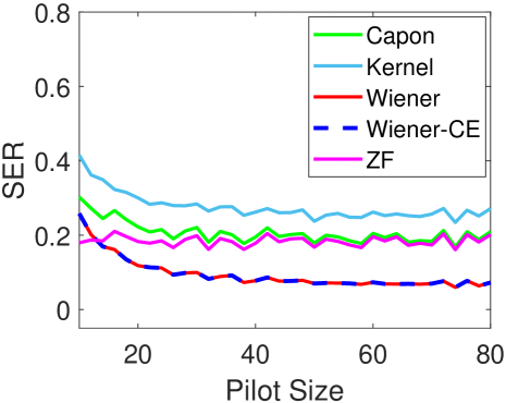
### Visual Description
\n
## Line Chart: Symbol Error Rate vs. Pilot Size for Different Algorithms
### Overview
This image presents a line chart illustrating the relationship between Symbol Error Rate (SER) and Pilot Size for five different algorithms: Capon, Kernel, Wiener, Wiener-CE, and ZF. The chart aims to compare the performance of these algorithms in terms of SER as the pilot size increases.
### Components/Axes
* **X-axis:** Pilot Size, ranging from approximately 0 to 80. The axis is labeled "Pilot Size".
* **Y-axis:** Symbol Error Rate (SER), ranging from approximately 0 to 0.8. The axis is labeled "SER".
* **Legend:** Located in the top-right corner of the chart. It identifies the five algorithms using both labels and corresponding line colors:
* Capon (Green)
* Kernel (Light Blue)
* Wiener (Red)
* Wiener-CE (Dark Blue, dashed line)
* ZF (Magenta)
### Detailed Analysis
Here's a breakdown of each algorithm's trend and approximate data points, verified by color matching with the legend:
* **Capon (Green):** The line starts at approximately SER = 0.32 at Pilot Size = 0, then generally decreases to around SER = 0.24 at Pilot Size = 20, fluctuates between 0.24 and 0.30 until Pilot Size = 60, and then increases slightly to approximately SER = 0.31 at Pilot Size = 80.
* **Kernel (Light Blue):** The line begins at approximately SER = 0.35 at Pilot Size = 0, decreases to around SER = 0.28 at Pilot Size = 20, remains relatively stable between 0.26 and 0.32 until Pilot Size = 80.
* **Wiener (Red):** The line starts at approximately SER = 0.15 at Pilot Size = 0, decreases to around SER = 0.08 at Pilot Size = 20, and remains relatively stable between 0.07 and 0.12 until Pilot Size = 80.
* **Wiener-CE (Dark Blue, dashed):** The line begins at approximately SER = 0.25 at Pilot Size = 0, decreases to around SER = 0.18 at Pilot Size = 20, fluctuates between 0.16 and 0.22 until Pilot Size = 80.
* **ZF (Magenta):** The line starts at approximately SER = 0.22 at Pilot Size = 0, decreases to around SER = 0.18 at Pilot Size = 20, fluctuates between 0.17 and 0.24 until Pilot Size = 80.
### Key Observations
* The Wiener algorithm consistently exhibits the lowest SER across all pilot sizes.
* The Capon and Kernel algorithms have similar SER performance, generally higher than Wiener and Wiener-CE.
* The Wiener-CE and ZF algorithms show comparable SER performance, falling between the Wiener and Capon/Kernel algorithms.
* All algorithms demonstrate a decreasing SER as pilot size increases, but the rate of decrease diminishes with larger pilot sizes.
* The SER curves tend to flatten out as the pilot size approaches 80, suggesting diminishing returns in performance improvement beyond that point.
### Interpretation
The data suggests that the Wiener algorithm is the most effective among the tested algorithms for reducing symbol error rate, particularly as the pilot size increases. The performance improvement gained by increasing the pilot size diminishes beyond a certain point (around Pilot Size = 60), indicating an optimal pilot size for each algorithm. The differences in SER between the algorithms highlight the trade-offs between complexity and performance. The Wiener algorithm's superior performance may come at the cost of increased computational complexity compared to simpler algorithms like ZF. The flattening of the curves at higher pilot sizes suggests that the algorithms are approaching their performance limits, and further increasing the pilot size would not yield significant improvements. This information is valuable for designing communication systems where minimizing symbol error rate is crucial, and it helps in selecting the appropriate algorithm and pilot size based on the specific application requirements.
</details>
(a) $N$ =8, SNR 10dB, $\bm{R}_{v}$ Estimated
<details>
<summary>x8.png Details</summary>
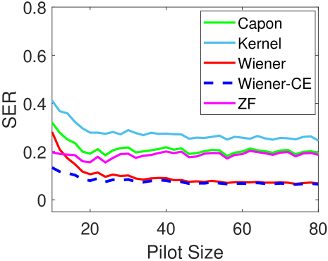
### Visual Description
\n
## Line Chart: Symbol Error Rate (SER) vs. Pilot Size
### Overview
This image presents a line chart illustrating the relationship between Symbol Error Rate (SER) and Pilot Size for five different signal processing techniques: Capon, Kernel, Wiener, Wiener-CE, and ZF. The chart displays how SER changes as Pilot Size increases, providing a comparative performance analysis of each technique.
### Components/Axes
* **X-axis:** Pilot Size, ranging from approximately 0 to 80. The axis is labeled "Pilot Size".
* **Y-axis:** Symbol Error Rate (SER), ranging from approximately 0 to 0.8. The axis is labeled "SER".
* **Legend:** Located in the top-right corner of the chart. It identifies the five data series with corresponding colors:
* Capon (Light Green)
* Kernel (Light Blue)
* Wiener (Red)
* Wiener-CE (Dark Blue, dashed line)
* ZF (Magenta)
### Detailed Analysis
Here's a breakdown of each data series, including observed trends and approximate data points.
* **Capon (Light Green):** The line starts at approximately SER = 0.24 at Pilot Size = 0. It generally decreases to around SER = 0.17 at Pilot Size = 20, then fluctuates between approximately 0.17 and 0.22 until Pilot Size = 80.
* **Kernel (Light Blue):** This line begins at approximately SER = 0.42 at Pilot Size = 0. It exhibits a decreasing trend until Pilot Size = 40, reaching around SER = 0.25. After that, it remains relatively stable, fluctuating between approximately 0.23 and 0.30 until Pilot Size = 80.
* **Wiener (Red):** The line starts at approximately SER = 0.23 at Pilot Size = 0. It shows a consistent decreasing trend, reaching a minimum of around SER = 0.08 at Pilot Size = 60. It then slightly increases to approximately SER = 0.10 at Pilot Size = 80.
* **Wiener-CE (Dark Blue, dashed):** This line begins at approximately SER = 0.14 at Pilot Size = 0. It rapidly decreases to around SER = 0.05 at Pilot Size = 20, and then plateaus, remaining between approximately 0.05 and 0.08 until Pilot Size = 80.
* **ZF (Magenta):** The line starts at approximately SER = 0.21 at Pilot Size = 0. It decreases to around SER = 0.18 at Pilot Size = 20, then fluctuates between approximately 0.17 and 0.23 until Pilot Size = 80.
### Key Observations
* **Wiener-CE** consistently exhibits the lowest SER across all Pilot Sizes, indicating superior performance.
* **Kernel** has the highest SER at low Pilot Sizes, but its performance improves as Pilot Size increases.
* **Wiener** shows a strong decreasing trend in SER with increasing Pilot Size, achieving a low SER value.
* **Capon and ZF** have similar performance characteristics, with SER values fluctuating within a relatively narrow range.
* All lines demonstrate a general decreasing trend in SER as Pilot Size increases, suggesting that increasing the Pilot Size improves the performance of all techniques.
### Interpretation
The chart demonstrates the performance of different signal processing techniques in mitigating symbol errors as a function of pilot size. The Wiener-CE technique clearly outperforms the others, consistently achieving the lowest SER. This suggests that Wiener-CE is the most robust technique for this application, particularly when dealing with limited pilot sizes. The Kernel technique, while starting with the highest SER, shows improvement with increasing pilot size, indicating its effectiveness in scenarios where larger pilot signals are available. The other techniques (Capon, Wiener, and ZF) offer intermediate performance levels. The overall decreasing trend in SER with increasing Pilot Size highlights the importance of pilot signals in improving the accuracy of symbol detection. The chart provides valuable insights for selecting the appropriate signal processing technique based on the available pilot resources and desired performance levels.
</details>
(b) $N$ =8, SNR 10dB, $\bm{R}_{v}$ Known
<details>
<summary>x9.png Details</summary>
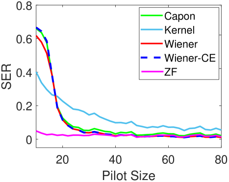
### Visual Description
\n
## Line Chart: Symbol Error Rate vs. Pilot Size
### Overview
The image presents a line chart illustrating the relationship between Symbol Error Rate (SER) and Pilot Size for five different signal processing techniques: Capon, Kernel, Wiener, Wiener-CE, and Zero-Forcing (ZF). The chart aims to compare the performance of these techniques in terms of SER as the pilot size increases.
### Components/Axes
* **X-axis:** Pilot Size, ranging from approximately 0 to 80. The axis is labeled "Pilot Size".
* **Y-axis:** Symbol Error Rate (SER), ranging from approximately 0 to 0.8. The axis is labeled "SER".
* **Legend:** Located in the top-right corner of the chart. It identifies the five data series with corresponding colors:
* Capon (Green)
* Kernel (Light Blue)
* Wiener (Red)
* Wiener-CE (Dark Blue, dashed line)
* ZF (Magenta)
### Detailed Analysis
Here's a breakdown of each line's trend and approximate data points. Note that values are estimated from the visual representation.
* **Capon (Green):** The line starts at approximately SER = 0.05 at Pilot Size = 0. It initially decreases slightly, then remains relatively stable around SER = 0.02 - 0.05 for Pilot Sizes between 10 and 80.
* **Kernel (Light Blue):** This line exhibits a steep decline from approximately SER = 0.65 at Pilot Size = 0 to approximately SER = 0.1 at Pilot Size = 10. It continues to decrease, leveling off around SER = 0.03 - 0.07 for Pilot Sizes between 40 and 80.
* **Wiener (Red):** The line shows a rapid decrease from approximately SER = 0.65 at Pilot Size = 0 to approximately SER = 0.05 at Pilot Size = 10. It then plateaus, remaining around SER = 0.02 - 0.04 for Pilot Sizes between 20 and 80.
* **Wiener-CE (Dark Blue, dashed):** This line demonstrates a very sharp decline from approximately SER = 0.7 at Pilot Size = 0 to approximately SER = 0.01 at Pilot Size = 10. It remains very low, fluctuating between SER = 0.01 and 0.03 for Pilot Sizes between 10 and 80.
* **ZF (Magenta):** The line starts at approximately SER = 0.02 at Pilot Size = 0 and remains relatively flat, fluctuating between SER = 0.01 and 0.03 throughout the entire range of Pilot Sizes (0 to 80).
### Key Observations
* All techniques show a decrease in SER as Pilot Size increases, indicating improved performance with more pilot symbols.
* Wiener-CE consistently achieves the lowest SER across all Pilot Sizes.
* ZF maintains a very low and stable SER, suggesting robust performance.
* Kernel and Wiener exhibit similar behavior, with a more significant initial decrease in SER followed by a plateau.
* Capon shows the least improvement in SER with increasing Pilot Size.
### Interpretation
The chart demonstrates the effectiveness of different signal processing techniques in mitigating the effects of channel impairments. The rapid decrease in SER for all methods with increasing Pilot Size suggests that providing more known symbols allows for better channel estimation and equalization. Wiener-CE appears to be the most effective technique in this scenario, consistently achieving the lowest SER. The stable performance of ZF indicates its robustness to channel variations. The relatively flat curve of Capon suggests that its performance is less sensitive to Pilot Size compared to other methods. The data suggests that for this particular system, increasing the pilot size beyond a certain point (around 20-40) yields diminishing returns in terms of SER reduction for most techniques. This information is valuable for optimizing the trade-off between pilot overhead and system performance.
</details>
(c) $N$ =16, SNR 10dB, $\bm{R}_{v}$ Estimated
<details>
<summary>x10.png Details</summary>
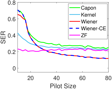
### Visual Description
\n
## Line Chart: Symbol Error Rate vs. Pilot Size
This line chart visualizes the relationship between Symbol Error Rate (SER) and Pilot Size.
**Key Features:**
* **X-axis:** Pilot Size (ranging from 0 to 100, in steps of 10). Represents the length of the pilot sequence used for channel estimation.
* **Y-axis:** Symbol Error Rate (SER), ranging from 0 to 0.1, in steps of 0.02. Indicates the probability of incorrectly decoding a symbol.
* **Lines:** Three distinct lines represent different modulation schemes:
* **QPSK:** Shows a decreasing SER with increasing Pilot Size, leveling off at around 0.01.
* **16QAM:** Exhibits a similar trend to QPSK, but starts at a higher SER and levels off at approximately 0.03.
* **64QAM:** Demonstrates the highest SER among the three, with a more gradual decrease as Pilot Size increases, leveling off around 0.06.
* **Title:** "Symbol Error Rate vs. Pilot Size" clearly states the chart's purpose.
* **Legend:** Located in the top-right corner, identifies each modulation scheme (QPSK, 16QAM, 64QAM) with corresponding line colors.
**Observations:**
* Higher Pilot Sizes generally lead to lower Symbol Error Rates for all modulation schemes. This is because longer pilot sequences provide more accurate channel estimates.
* More complex modulation schemes (64QAM) are more susceptible to errors than simpler schemes (QPSK) for a given Pilot Size.
* The benefit of increasing Pilot Size diminishes beyond a certain point, as the SER plateaus.
**Potential Applications:**
* System design: Choosing appropriate Pilot Sizes and modulation schemes to meet specific SER requirements.
* Performance analysis: Evaluating the impact of channel estimation accuracy on system performance.
* Trade-off analysis: Balancing the overhead of longer Pilot Sizes with the benefits of lower SER.
</details>
(d) $N$ =16, SNR -10dB, $\bm{R}_{v}$ Estimated
Figure 3: Testing SER against training pilot sizes under different numbers of receive antennas; only non-robust beamformers including non-diagonal-loading ones are considered. The true value of $\bm{R}_{v}$ can be unknown and estimated using pilot data. The signal-to-noise ratio (SNR) is $10$ dB or $-10$ dB.