2402.01825

# Fractal Patterns May Illuminate the Success of Next-Token Prediction **Authors**: - Ibrahim Alabdulmohsin (Google Deepmind) - Zürich, Switzerland - &Vinh Q. Tran (Google Deepmind) - New York, USA - &Mostafa Dehghani (Google Deepmind) - Mountain View, USA > Corresponding author. Abstract We study the fractal structure of language, aiming to provide a precise formalism for quantifying properties that may have been previously suspected but not formally shown. We establish that language is: (1) self-similar, exhibiting complexities at all levels of granularity, with no particular characteristic context length, and (2) long-range dependent (LRD), with a Hurst parameter of approximately $\mathrm{H}=0.70± 0.09$ . Based on these findings, we argue that short-term patterns/dependencies in language, such as in paragraphs, mirror the patterns/dependencies over larger scopes, like entire documents. This may shed some light on how next-token prediction can capture the structure of text across multiple levels of granularity, from words and clauses to broader contexts and intents. In addition, we carry out an extensive analysis across different domains and architectures, showing that fractal parameters are robust. Finally, we demonstrate that the tiny variations in fractal parameters seen across LLMs improve upon perplexity-based bits-per-byte (BPB) in predicting their downstream performance. We hope these findings offer a fresh perspective on language and the mechanisms underlying the success of LLMs. 1 Introduction How does the training objective of predicting the next token in large language models (LLMs) yield remarkable capabilities? Consider, for instance, the two models: Gemini [5] and GPT4 [49]. These models have demonstrated capabilities that extend to quantitative reasoning, summarization, and even coding, which has led some researchers to ponder if there was more to intelligence than “on-the-fly improvisation” [11]. While providing a satisfactory explanation is a difficult endeavor, a possible insight can be drawn from fractals and self-similarity. We elucidate the connection in this work. Self-Similarity. Self-similar processes were introduced by Kolmogorov in 1940 [36]. The notion garnered considerable attention during the late 1960s, thanks to the extensive works of Mandelbrot and his peers [19]. Broadly speaking, an object is called “self-similar” if it is invariant across scales, meaning its statistical or geometric properties stay consistent irrespective of the magnification applied to it (see Figure 1). Nature and geometry furnish us with many such patterns, such as coastlines, snowflakes, the Cantor set and the Kuch curve. Despite the distinction, self-similarity is often discussed in the context of “fractals,” another term popularized by Mandelbrot in his seminal book The Fractal Geometry of Nature [44]. However, the two concepts are different [26]. See Section 2. In language, in particular, there have been studies arguing for the presence of a self-similar structure. Nevertheless, due to computational constraints, it was not feasible to holistically model the joint probability distribution of language. As such, linguists often resorted to rudimentary approximations in their arguments, such as by substituting a word with its frequency or length [9], or by focusing on the recurrence of a specific, predetermined word [48, 3]. These studies fall short of fully capturing the structure of language due to the simplifying assumptions they make, as discussed in Section 4. Highlighting the self-similar nature of a process can have profound implications. For instance, conventional Poisson models for Ethernet traffic were shown to fail because traffic was self-similar [16, 38, 50, 66]. In such cases, recognizing and quantifying self-similarity had practical applications, such as in the design of buffers [39]. Similarly in language, we argue that self-similarity may offer a fresh perspective on the mechanisms underlying the success of LLMs. Consider the illustrative example shown in Figure 1, where the task is to predict the subsequent measurement in a time series, specifically predicting next tokens in a Wikipedia article (see Section 2 for details). The three plots in Figure 1 (left) represent different manifestations of the same process observed across three distinct time scales. Notably, we observe rich, self-similar details, such as burstiness, in all of them. A well-established approach for quantifying self-similarity is the Hölder exponent [64], which we denote by $\mathrm{S}$ . In language, we find it to be $\mathrm{S}=0.59± 0.08$ , confirming statistical self-similarity. Figure 1: Manifestations of processes across different time scales. A region marked in red corresponds to the magnified plot beneath it. left: The process exhibits self-similarity with rich details at all levels of granularity. It is an integral process $(X_{t})_{t∈\mathbb{N}}$ calculated from Wikipedia (see Section 2). right: Example of a process that is not self-similar, looking smoother at larger time scales. Why is this important? We hypothesize that since LLMs are trained to predict the future of a self-similar process, they develop proficiency in capturing patterns across multiple levels of granularity for two interconnected reasons. First, self-similarity implies that the patterns at the level of a paragraph are reflective of the patterns seen at the level of a whole text, which is reminiscent of the recursive structure of language [52]. Thus, recognizing short-term patterns can aide in learning broader contexts. Second, because language displays intricate patterns at all levels of granularity, it would not be enough to rely only on the immediate context of a sentence to predict the next token. Instead, the model needs to identify patterns at higher levels of granularity; e.g. follow the direction of the argument and the broader intent. It must balance between short- and long-term contexts. Willinger et al., [65] and Altmann et al., [3] argue for self-similarity in language due to this hierarchical nature. Long-range dependence. However, self-similarity alone is not sufficient for a predictive model to exhibit anything resembling “intelligent” behavior. In fact, some self-similar processes, despite their intricate details, remain entirely unpredictable. A quintessential example is the simple Brownian motion, which is a Wiener process with independent increments. Its discrete analog is $B_{n}=\sum_{i=1}^{n}\varepsilon_{i}$ , where $\varepsilon_{i}\sim\mathcal{N}(0,\sigma^{2})$ . Despite possessing rich details at all granularities, a model trained to predict $B_{n}$ cannot learn anything useful from data since the process itself has independent increments. Thus, for strong capabilities to emerge, the process must have some degree of predictability or dependence as well. One classical metric for quantifying predictability in a stochastic process is the Hurst parameter [31], developed by the hydrologist H. E. Hurst in 1951 while studying the Nile river. It is generally considered to be a robust metric [65], unlike the wavelet estimator [1] and the periodogram method [24] that can be sensitive to errors [53]. As discussed in Section 2.3, we find the Hurst parameter in language to be $\mathrm{H}=0.70± 0.09$ . For context, $\mathrm{H}$ only takes values in $[0,1]$ . A value $\mathrm{H}>0.5$ implies predictability in the data, while $\mathrm{H}=0.5$ indicates random increments. While it is compelling that our estimate of $\mathrm{H}$ in language lies nearly midway between predictability ( $\mathrm{H}=1$ ) and noise ( $\mathrm{H}=0.5$ ), a Hurst parameter of about $0.75$ turns out to occur commonly in nature, including in river discharges, Ethernet traffic, temperatures, precipitation, and tree rings [16, 21, 8]. For agents that learn from data, such as LLMs, this value is also reminiscent of processing-based theories of curiosity, which suggest that a sweet spot of complexity exists (not too simple, nor too unpredictable) that facilities or accelerates learning [34]. Importantly, predictability and self-similarity together imply long-range dependence (LRD). This follows from the definition of self-similarity, where the patterns at small scales mirror those at larger scales so, for example, the correlations established at micro levels are also pertinent at macro levels. LRD is arguably crucial for enhancing the functionality of predictive models because processes with only short-range dependence could be forecasted (somewhat trivially) with lookup tables that provide the likelihood of transitions over brief sequences. By contrast, this is not possible in LRD processes whose contexts extend indefinitely into the past. Information Theoretic Complexity. To define fractal parameters, we follow recent works such as [28, 22, 40, 46, 25] in adopting an information-theoretic characterization of the complexity in language using minimal-length codes or surprise. This corresponds to an intrinsic, irreducible description of language and the minimum compute overhead to comprehend/decode it [22], which also correlates well with actual reading times [28, 40]. In this context, self-similarity means that the intrinsic complexity or surprise in language (measured in bits) cannot be smoothed out, even as we look into broader narratives. That is, surprising paragraphs will follow predictable paragraphs, in a manner that is statistically similar to how surprising sentences follow predictable sentences. Analysis. How robust are these findings? To answer this question, we carry out an extensive empirical analysis across various model architectures and scales, ranging from 1B to over 500B parameters. We find that fractal parameters are quite robust to the choice of the architecture. However, there exists tiny variations across LLMs. Interestingly, we demonstrate that from a practical standpoint, these differences help in predicting downstream performance in LLMs compared to using perplexity-based metrics alone, such as bits-per-byte (BPB). Specifically, we introduce a new metric and show that using it to predict downstream performance can increase the adjusted $R^{2}$ from approximately $0.65$ when using solely BPB, to over $0.86$ with the new metric We release the code for calculating fractal parameters at: https://github.com/google-research/google-research/tree/master/fractals_language . Statement of Contribution. In summary, we: 1. highlight how the fractal structure of language can offer a new perspective on the capabilities of LLMs, and provide a formalism to quantify properties, such as long-range dependence. 1. establish that language is self-similar and long-range dependent. We provide concrete estimates in language of the three parameters: the self-similarity (Hölder) exponent, the Hurst parameter, and the fractal dimension. We also estimate the related Joseph exponent. 1. carry out a comparative study across different model architectures and scales, and different domains, such as ArXiv and GitHub, demonstrating that fractal parameters are robust. 1. connect fractal patterns with learning. Notably, we show that a “median” Hurst exponent improves upon perplexity-based bits-per-byte (BPB) in predicting downstream performance. 2 Fractal Structure of Language 2.1 Preliminaries Suppose we have a discrete-time, stationary stochastic process $(x_{t})_{t∈\mathbb{N}}$ , with $\mathbb{E}[x_{t}]=0$ and $\mathbb{E}[x_{t}^{2}]=1$ . We will refer to $(x_{t})_{t∈\mathbb{N}}$ as the increment process to distinguish it from the integral process $(X_{t})_{t∈\mathbb{N}}$ defined by $X_{t}=\sum_{k=0}^{t}x_{k}$ . While $(x_{t})_{t∈\mathbb{N}}$ and $(X_{t})_{t∈\mathbb{N}}$ are merely different representations of the same data, it is useful to keep both representations in mind. For example, self-similarity is typically studied in the context of integral processes whereas LRD is defined on increment processes. In the literature, it is not uncommon to mistakenly equate parameters that are generally different. For example, the Hurst parameter $\mathrm{H}$ has had many definitions in the past that were not equivalent, and Mandelbrot himself cautioned against this [43]. The reason behind this is because different parameters can agree in the idealized fractional Brownian motion, leading some researchers to equate them in general [64]. We will keep the self-similarity exponent $\mathrm{S}$ and $\mathrm{H}$ separate in our discussion. <details> <summary>extracted/2402.01825v2/figs/selfsim/self_sim_exponent_lag_OpenWebText2.png Details</summary>  ### Visual Description # Technical Data Extraction: OpenWeb Log-Log Plot ## 1. Component Isolation * **Header:** Contains the title "OpenWeb". * **Main Chart:** A log-log scatter plot with a linear regression line. * **Axes:** * **Y-axis (Vertical):** Labeled "$p$", representing a probability or density. * **X-axis (Horizontal):** Labeled "$\tau$" (tau), representing a time constant or interval. ## 2. Axis Configuration and Scale The chart utilizes a logarithmic scale (base 10) for both axes, indicating a power-law relationship between the variables. * **Y-axis ($p$):** * Range: $10^{-5}$ to $10^{-3}$. * Major markers: $10^{-5}$, $10^{-4}$, $10^{-3}$. * A faint horizontal grid line is present at the $10^{-4}$ level. * **X-axis ($\tau$):** * Range: $10^1$ (10) to $10^3$ (1000). * Major markers: $10^1$, $10^3$. * The midpoint between $10^1$ and $10^3$ (which would be $10^2$ or 100) is not explicitly labeled but is visually the center of the axis. ## 3. Data Series Analysis ### Series 1: Observed Data Points (Blue Circles) * **Visual Trend:** The data points form a downward-sloping linear pattern on the log-log scale. This confirms a negative power-law correlation. * **Spatial Distribution:** There are 7 distinct blue circular data points. * **Estimated Data Points:** | Point | $\tau$ (approx) | $p$ (approx) | | :--- | :--- | :--- | | 1 | $2 \times 10^1$ | $8 \times 10^{-4}$ | | 2 | $4 \times 10^1$ | $4 \times 10^{-4}$ | | 3 | $7 \times 10^1$ | $2 \times 10^{-4}$ | | 4 | $1 \times 10^2$ | $1 \times 10^{-4}$ | | 5 | $2 \times 10^2$ | $5 \times 10^{-5}$ | | 6 | $4 \times 10^2$ | $2 \times 10^{-5}$ | | 7 | $7 \times 10^2$ | $1 \times 10^{-5}$ | ### Series 2: Regression Line (Red Solid Line) * **Description:** A solid red line passes through the center of the data points, representing the best-fit power-law model. * **Slope:** The slope is negative, consistent with the decay of $p$ as $\tau$ increases. </details> <details> <summary>extracted/2402.01825v2/figs/selfsim/self_sim_exponent_lag_Github.png Details</summary>  ### Visual Description # Technical Document Extraction: Github Data Plot ## 1. Component Isolation * **Header:** Contains the title "Github". * **Main Chart Area:** A log-log scatter plot with a linear regression line. * **Axes:** * **Y-axis (Vertical):** Labeled "$p$". * **X-axis (Horizontal):** Labeled "$\tau$". ## 2. Metadata and Labels * **Title:** Github * **Y-axis Label:** $p$ (representing probability or a related density metric). * **X-axis Label:** $\tau$ (tau, representing a time interval or scale). * **Y-axis Scale:** Logarithmic, ranging from $10^{-5}$ to $10^{-3}$. Major tick marks are at $10^{-5}$, $10^{-4}$, and $10^{-3}$. * **X-axis Scale:** Logarithmic, ranging from $10^1$ to $10^3$. Major tick marks are at $10^1$ and $10^3$. ## 3. Data Series Analysis ### Trend Verification * **Blue Data Points:** There are 8 circular blue data points. They follow a clear downward linear trend on the log-log scale, indicating a power-law relationship between $p$ and $\tau$. * **Red Regression Line:** A solid red line passes through the center of the blue data points. The line slopes downward from the top-left toward the bottom-right. ### Data Point Extraction (Estimated from Log Scale) The data points are clustered between $\tau \approx 50$ and $\tau \approx 700$. | Point | $\tau$ (X-axis approx.) | $p$ (Y-axis approx.) | | :--- | :--- | :--- | | 1 | 60 | $3 \times 10^{-4}$ | | 2 | 80 | $2.2 \times 10^{-4}$ | | 3 | 100 | $1.8 \times 10^{-4}$ | | 4 | 150 | $1.2 \times 10^{-4}$ | | 5 | 200 | $1.0 \times 10^{-4}$ | | 6 | 300 | $0.9 \times 10^{-4}$ | | 7 | 500 | $0.7 \times 10^{-4}$ | | 8 | 700 | $0.6 \times 10^{-4}$ | ## 4. Visual Components and Flow * **Gridlines:** A single horizontal grey gridline is visible at the $p = 10^{-4}$ mark. * **Relationship:** The plot illustrates that as $\tau$ increases, $p$ decreases. Because this is a straight line on a log-log plot, it represents a functional form of $p(\tau) \propto \tau^{-\alpha}$, where $\alpha$ is the absolute value of the slope of the red line. * **Spatial Grounding:** * The title "Github" is centered at the top. * The Y-axis label "$p$" is centered vertically on the left. * The X-axis label "$\tau$" is centered horizontally at the bottom. * The data points are concentrated in the upper-middle to center-right region of the plot area. ## 5. Language Declaration The text in this image is entirely in **English** (Title) and **Mathematical Notation** (Greek letter $\tau$, variable $p$, and scientific notation for powers of 10). No other languages are present. </details> <details> <summary>extracted/2402.01825v2/figs/selfsim/self_sim_exponent_lag_FreeLaw.png Details</summary>  ### Visual Description # Technical Document Extraction: FreeLaw Data Plot ## 1. Component Isolation * **Header:** Contains the title "FreeLaw". * **Main Chart Area:** A log-log scatter plot with a superimposed linear regression line. * **Axes:** * **Y-axis (Vertical):** Labeled "$p$". * **X-axis (Horizontal):** Labeled "$\tau$". ## 2. Metadata and Labels | Element | Value | | :--- | :--- | | **Title** | FreeLaw | | **Y-axis Label** | $p$ | | **X-axis Label** | $\tau$ | | **Y-axis Scale** | Logarithmic ($10^{-5}$ to $10^{-3}$) | | **X-axis Scale** | Logarithmic ($10^{1}$ to $10^{3}$) | | **Language** | English | ## 3. Data Series Analysis ### Series 1: Observed Data Points * **Visual Representation:** Large blue circular markers. * **Trend Verification:** The data points follow a clear downward slope from left to right. As $\tau$ increases, $p$ decreases. The points are tightly clustered around a straight line on this log-log scale, indicating a power-law relationship. * **Estimated Data Points (Logarithmic Scale):** * Point 1: $\tau \approx 50, p \approx 3 \times 10^{-4}$ * Point 2: $\tau \approx 70, p \approx 2.5 \times 10^{-4}$ * Point 3: $\tau \approx 100, p \approx 2 \times 10^{-4}$ * Point 4: $\tau \approx 200, p \approx 1.5 \times 10^{-4}$ * Point 5: $\tau \approx 300, p \approx 1.3 \times 10^{-4}$ * Point 6: $\tau \approx 500, p \approx 1 \times 10^{-4}$ * Point 7: $\tau \approx 800, p \approx 8 \times 10^{-5}$ ### Series 2: Trend Line * **Visual Representation:** Solid red line. * **Trend Verification:** Slopes downward. It acts as a "best fit" line for the blue data points. * **Placement:** The line originates near the top-left corner ($10^1, 10^{-3}$) and terminates near the bottom-right corner ($10^3, 5 \times 10^{-5}$). ## 4. Axis Markers and Grid * **Y-axis Ticks:** $10^{-3}$, $10^{-4}$, $10^{-5}$. There is a faint horizontal grid line at the $10^{-4}$ mark. * **X-axis Ticks:** $10^{1}$, $10^{3}$. (Note: $10^2$ is implied in the center but not explicitly labeled). ## 5. Summary of Information The image represents a scientific or statistical analysis titled **FreeLaw**. It illustrates the relationship between two variables, $\tau$ (tau) and $p$. Because the data forms a straight line on a log-log plot, it demonstrates that $p$ is proportional to $\tau$ raised to a negative power ($p \propto \tau^{-k}$). The blue markers represent empirical data, while the red line represents the theoretical or fitted model. The values for $p$ range between $10^{-3}$ and $10^{-5}$ as $\tau$ scales from $10^1$ to $10^3$. </details> <details> <summary>extracted/2402.01825v2/figs/selfsim/self_sim_exponent_lag_Pile-CC.png Details</summary>  ### Visual Description # Technical Document Extraction: PileCC Log-Log Plot ## 1. Component Isolation * **Header:** Contains the title "PileCC". * **Main Chart Area:** A log-log scale scatter plot with a superimposed linear regression line. * **Axes:** * **Y-axis (Vertical):** Labeled "$p$", representing a probability or proportion. * **X-axis (Horizontal):** Labeled "$\tau$" (tau), representing a time constant or interval. --- ## 2. Metadata and Labels | Element | Label/Value | Description | | :--- | :--- | :--- | | **Title** | PileCC | The dataset or experiment identifier. | | **Y-axis Label** | $p$ | Probability or proportion metric. | | **X-axis Label** | $\tau$ | Time constant or interval metric. | </details> <details> <summary>extracted/2402.01825v2/figs/selfsim/self_sim_exponent_lag_Wikipediaen.png Details</summary>  ### Visual Description # Technical Data Extraction: Log-Log Plot "Wiki" ## 1. Component Isolation * **Header:** Contains the title "Wiki". * **Main Chart Area:** A log-log coordinate system featuring a series of data points and a linear regression line. * **Axes:** * **Y-axis (Vertical):** Labeled "$p$". * **X-axis (Horizontal):** Labeled "$\tau$". ## 2. Axis Configuration and Scale The chart uses a logarithmic scale for both the x and y axes (Log-Log plot). * **Y-axis ($p$):** * Range: $10^{-5}$ to $10^{-3}$. * Major Ticks: $10^{-5}$, $10^{-4}$, $10^{-3}$. * A faint horizontal grid line is present at the $10^{-4}$ level. * **X-axis ($\tau$):** * Range: $10^{1}$ (10) to $10^{3}$ (1000). * Major Ticks: $10^{1}$, $10^{3}$. (Note: $10^2$ is implied by the spacing but not explicitly labeled). ## 3. Data Series and Trend Verification There are two primary visual elements within the plot area: 1. **Data Points (Blue Circles):** * **Visual Trend:** The points follow a downward-sloping linear path on the log-log scale, indicating a power-law relationship between $p$ and $\tau$. * **Quantity:** There are 7 distinct blue circular markers. 2. **Regression Line (Red Solid Line):** * **Visual Trend:** Slopes downward from the top-left toward the bottom-right. * **Fit:** The line acts as a "best fit" through the center of the blue data points. ## 4. Data Point Extraction (Estimated) Based on the logarithmic scales, the approximate coordinates for the 7 data points are as follows: | Point | $\tau$ (x-axis) | $p$ (y-axis) | | :--- | :--- | :--- | | 1 | ~50 | ~3.0 x $10^{-4}$ | | 2 | ~70 | ~2.5 x $10^{-4}$ | | 3 | ~100 | ~2.0 x $10^{-4}$ | | 4 | ~150 | ~1.5 x $10^{-4}$ | | 5 | ~200 | ~1.1 x $10^{-4}$ | | 6 | ~300 | ~1.0 x $10^{-4}$ | | 7 | ~600 | ~0.6 x $10^{-4}$ | ## 5. Summary of Information The image represents a statistical distribution for a dataset labeled **"Wiki"**. It illustrates that the variable **$p$** decreases as the variable **$\tau$** increases. Because the relationship is linear on a log-log plot, it suggests a power-law decay of the form $p \propto \tau^{-\alpha}$. The data points are tightly clustered around the red regression line, indicating a high degree of correlation for the observed range of $\tau$ (approximately 50 to 600). </details> <details> <summary>extracted/2402.01825v2/figs/selfsim/self_sim_exponent_lag_PubMedCentral.png Details</summary>  ### Visual Description # Technical Document Extraction: PubMed Data Plot ## 1. Component Isolation * **Header:** Contains the title "PubMed". * **Main Chart Area:** A log-log scatter plot with a linear regression line. * **Axes:** * **Y-axis (Vertical):** Labeled "$p$". * **X-axis (Horizontal):** Labeled "$\tau$". ## 2. Metadata and Labels * **Title:** PubMed * **Y-axis Label:** $p$ (likely representing probability or a density function). * **X-axis Label:** $\tau$ (tau, likely representing a time interval or scale). * **Y-axis Scale:** Logarithmic, ranging from $10^{-5}$ to $10^{-3}$. Major tick marks are visible at $10^{-5}$, $10^{-4}$, and $10^{-3}$. * **X-axis Scale:** Logarithmic, ranging from $10^1$ to $10^3$. Major tick marks are visible at $10^1$ and $10^3$. ## 3. Data Series Analysis The chart contains two primary visual elements representing data: ### Series 1: Observed Data Points * **Visual Description:** Seven blue circular markers. * **Trend Verification:** The points follow a consistent downward slope from left to right. * **Spatial Distribution:** The points are clustered between $x \approx 5 \times 10^1$ and $x \approx 7 \times 10^2$. | Point | Estimated $\tau$ (X-axis) | Estimated $p$ (Y-axis) | | :--- | :--- | :--- | | 1 | $\approx 60$ | $\approx 3 \times 10^{-4}$ | | 2 | $\approx 80$ | $\approx 2.5 \times 10^{-4}$ | | 3 | $\approx 100$ | $\approx 2 \times 10^{-4}$ | | 4 | $\approx 150$ | $\approx 1.6 \times 10^{-4}$ | | 5 | $\approx 200$ | $\approx 1.4 \times 10^{-4}$ | | 6 | $\approx 400$ | $\approx 1 \times 10^{-4}$ | | 7 | $\approx 700$ | $\approx 8 \times 10^{-5}$ | ### Series 2: Regression/Fit Line * **Visual Description:** A solid red line. * **Trend Verification:** The line slopes downward, indicating a power-law relationship ($p \propto \tau^{-\alpha}$). * **Placement:** The line passes directly through the center of the blue data points, acting as a "best fit" model. It extends from the left boundary ($10^1$) to the right boundary ($10^3$). * **Intercepts:** * At $\tau = 10^1$, $p \approx 8 \times 10^{-4}$. * At $\tau = 10^3$, $p \approx 5 \times 10^{-5}$. ## 4. Key Trends and Observations * **Power-Law Relationship:** Because the data forms a straight line on a log-log plot, it indicates a power-law distribution between the variables $\tau$ and $p$. * **Negative Correlation:** As the value of $\tau$ increases, the value of $p$ decreases at a constant scaling rate. * **Reference Line:** There is a faint horizontal grey grid line at $p = 10^{-4}$ which serves as a visual anchor for the data points. The data points cross this threshold at approximately $\tau = 400$. ## 5. Language Declaration * **Primary Language:** English. * **Symbols:** Greek letter $\tau$ (Tau) is used as a mathematical variable. </details> <details> <summary>extracted/2402.01825v2/figs/selfsim/self_sim_exponent_lag_DMMathematics.png Details</summary>  ### Visual Description # Technical Document Extraction: DMMath Log-Log Plot ## 1. Component Isolation * **Header:** Contains the title "DMMath". * **Main Chart Area:** A log-log coordinate system featuring a series of data points and a linear regression line. * **Axes:** * **Y-axis (Vertical):** Labeled "$p$". * **X-axis (Horizontal):** Labeled "$\tau$". ## 2. Metadata and Labels | Element | Value/Text | | :--- | :--- | | **Title** | DMMath | | **Y-Axis Label** | $p$ | | **X-Axis Label** | $\tau$ | | **Y-Axis Scale** | Logarithmic ($10^{-5}$ to $10^{-3}$) | | **X-Axis Scale** | Logarithmic ($10^{1}$ to $10^{3}$) | ## 3. Data Series Analysis The chart is a log-log plot, which typically illustrates power-law relationships where $p \propto \tau^{-k}$. ### Trend Verification * **Red Line:** Slopes downward from left to right. On a log-log scale, this linear trend represents a power-law decay. * **Blue Circular Markers:** These represent discrete data points. They follow the downward trajectory of the red line closely, indicating a strong correlation and a consistent decay rate. ### Data Point Extraction (Estimated) Based on the logarithmic grid: * **Point 1:** $\tau \approx 5 \times 10^1$, $p \approx 5 \times 10^{-4}$ * **Point 2:** $\tau \approx 7 \times 10^1$, $p \approx 4.5 \times 10^{-4}$ * **Point 3:** $\tau \approx 1 \times 10^2$, $p \approx 4 \times 10^{-4}$ * **Point 4:** $\tau \approx 2 \times 10^2$, $p \approx 3.5 \times 10^{-4}$ * **Point 5:** $\tau \approx 3 \times 10^2$, $p \approx 3 \times 10^{-4}$ * **Point 6:** $\tau \approx 5 \times 10^2$, $p \approx 2.5 \times 10^{-4}$ * **Point 7:** $\tau \approx 8 \times 10^2$, $p \approx 2 \times 10^{-4}$ ## 4. Visual Components and Flow 1. **Coordinate System:** The plot uses a square aspect ratio with major grid lines at powers of 10. A faint horizontal grid line is visible at $p = 10^{-4}$. 2. **Regression Line (Red):** The line originates near the top-left corner ($10^1, 10^{-3}$) and terminates near the bottom-right corner ($10^3, 1.5 \times 10^{-4}$). 3. **Data Points (Blue):** Seven large blue circular markers are plotted. They are clustered in the upper-right quadrant of the visible field, specifically between $\tau$ values of $5 \times 10^1$ and $8 \times 10^2$. ## 5. Summary of Information This image represents a technical data visualization for "DMMath". It shows a clear inverse relationship between the variable $\tau$ and the variable $p$. Because the data forms a straight line on a log-log scale, it confirms that $p$ decreases as a power of $\tau$. The data points are highly consistent with the fitted red regression line, suggesting a predictable mathematical model for the DMMath dataset. </details> <details> <summary>extracted/2402.01825v2/figs/selfsim/self_sim_exponent_lag_ArXiv.png Details</summary>  ### Visual Description # Technical Document Extraction: ArXiv Data Plot ## 1. Component Isolation * **Header:** Contains the title "ArXiv". * **Main Chart Area:** A log-log scatter plot with a superimposed linear regression line. * **Axes:** * **Y-axis (Vertical):** Labeled "$p$", representing a probability or density value. * **X-axis (Horizontal):** Labeled "$\tau$", representing a time-scale or interval. ## 2. Axis and Scale Information The chart utilizes a logarithmic scale (log-log) for both axes. * **Y-axis ($p$):** * **Range:** $10^{-5}$ to $10^{-3}$. * **Major Markers:** $10^{-5}$, $10^{-4}$, $10^{-3}$. * **Gridlines:** A faint horizontal gridline is present at the $10^{-4}$ mark. * **X-axis ($\tau$):** * **Range:** $10^{1}$ (10) to $10^{3}$ (1000). * **Major Markers:** $10^{1}$, $10^{3}$. * **Note:** The midpoint between $10^1$ and $10^3$ on a log scale is $10^2$ (100), which is where the data points are clustered. ## 3. Data Series Analysis ### Series 1: Observed Data (Blue Circles) * **Visual Trend:** The data points follow a strict downward linear slope on the log-log scale, indicating a power-law relationship ($p \propto \tau^{-\alpha}$). * **Spatial Grounding:** There are 7 distinct blue circular data points. * **Estimated Data Points:** 1. $\tau \approx 50, p \approx 3 \times 10^{-4}$ 2. $\tau \approx 70, p \approx 2.5 \times 10^{-4}$ 3. $\tau \approx 100, p \approx 2 \times 10^{-4}$ 4. $\tau \approx 150, p \approx 1.5 \times 10^{-4}$ 5. $\tau \approx 200, p \approx 1 \times 10^{-4}$ 6. $\tau \approx 300, p \approx 8 \times 10^{-5}$ 7. $\tau \approx 500, p \approx 6 \times 10^{-5}$ ### Series 2: Fit Line (Red Solid Line) * **Visual Trend:** A solid red line slopes downward from the top-left toward the bottom-right. * **Trend Verification:** The line acts as a "best fit" for the blue data points. It originates at $(\tau=10, p=10^{-3})$ and terminates near $(\tau=1000, p \approx 4 \times 10^{-5})$. * **Slope Observation:** Since the line drops roughly 1.4 orders of magnitude over 2 orders of magnitude on the x-axis, the power-law exponent $\alpha$ is approximately $0.7$. ## 4. Summary of Information | Feature | Description | | :--- | :--- | | **Dataset Name** | ArXiv | | **Plot Type** | Log-Log Scatter with Linear Fit | | **X-Axis Label** | $\tau$ (Tau) | | **Y-Axis Label** | $p$ | | **Relationship** | Inverse Power Law | | **Data Range ($\tau$)** | $\sim 50$ to $\sim 500$ | | **Data Range ($p$)** | $\sim 3 \times 10^{-4}$ to $\sim 6 \times 10^{-5}$ | **Conclusion:** The image illustrates a statistical distribution from ArXiv data where the variable $p$ decreases as $\tau$ increases, following a power-law decay. The alignment of the blue points with the red line suggests a high degree of correlation for the model in the observed range. 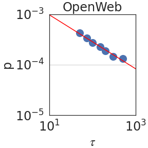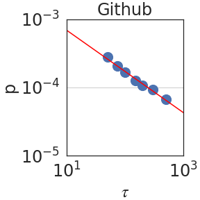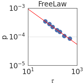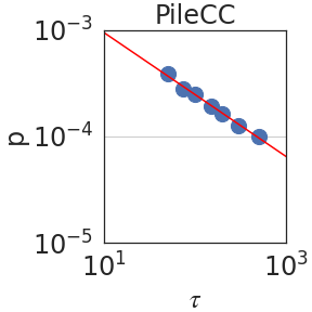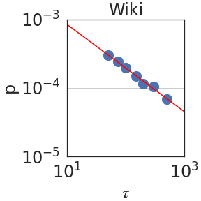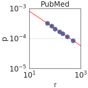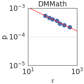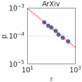</details> Figure 2: Peak probability $p_{\epsilon}(\tau)$ is plotted against the granularity level $\tau$ (see Section 2.2). We observe power laws $p_{\epsilon}(\tau)\sim\tau^{-\mathrm{S}}$ , indicating self-similarity, with a median exponent of $\mathrm{S}=0.59± 0.08$ . Experimental Setup. In order to establish self-similarity and LRD in language, we convert texts into sequences of bits using a large language model (LLM). Specifically, we use PaLM2-L (Unicorn) [6] to calculate the probability of the next token $w_{t}$ conditioned on its entire prefix $w_{[t-1]}=(w_{0},w_{1},...,w_{t-1})$ . As discussed in Section 1, this captures its intrinsic, irreducible description [22]. By the chain rule [15], the corresponding number of bits assigned to $w_{t}$ is $z_{t}=-\log p(w_{t}|w_{[t-1]})$ . Unlike in prior works, which rely on simplifications such as by substituting a word with its length [9] or by focusing on the recurrence of a single word [48, 3], we use the LLM to approximate the full joint distribution of language since LLMs are known to produce calibrated probability scores at the token level [33]. We carry out these calculations for prefixes of up to 2048 tokens ( $≈ 8$ pages of text). With a suitable normalization, such bits-per-byte (BPB), one obtains a standardized description of text, consistent across tokenizers. BPB is a widely used as a tokenizer-agnostic metric to compare LM modeling performance, e.g. for The Pile [23]. <details> <summary>extracted/2402.01825v2/figs/hurst/rs_exponent_rescaled_range_fit_OpenWebText2.png Details</summary>  ### Visual Description # Technical Document Extraction: OpenWeb Data Analysis ## 1. Image Overview This image is a log-log scatter plot with a linear regression line, representing data for "OpenWeb". It illustrates the relationship between a variable $n$ and a ratio $R/S$. ## 2. Component Isolation ### Header - **Title:** OpenWeb (Centered at the top of the chart area). ### Main Chart Area - **Type:** Log-Log Plot (both axes use logarithmic scales). - **Data Series 1 (Scatter):** Large blue circular markers. - **Data Series 2 (Trendline):** A solid red line passing through the data points. - **Gridlines:** Horizontal grey lines are visible at the major tick marks of the Y-axis ($10^1$ and $10^2$). ### Axis Labels and Markers - **X-axis (Horizontal):** - **Label:** $n$ (italicized). - **Markers:** $10^0$ (at the origin), $10^3$ (towards the right). - **Y-axis (Vertical):** - **Label:** $R/S$. - **Markers:** $10^0$ (at the origin), $10^1$, $10^2$, $10^3$ (top). ## 3. Trend Verification and Data Extraction ### Trend Analysis - **Visual Trend:** The blue data points follow a strictly positive, linear path on the log-log scale. This indicates a power-law relationship between $n$ and $R/S$. - **Red Line:** The red line slopes upward from the bottom-left toward the top-right, acting as a line of best fit for the blue markers. ### Data Point Estimation (Spatial Grounding) Given the logarithmic scale, the following approximations can be made based on the visual placement of the blue markers: | Data Point (Approx.) | $n$ (X-axis) | $R/S$ (Y-axis) | | :--- | :--- | :--- | | First Marker | $\approx 2 \times 10^2$ | $\approx 8 \times 10^0$ | | Second Marker | $\approx 3 \times 10^2$ | $\approx 1.2 \times 10^1$ | | Cluster Start | $\approx 5 \times 10^2$ | $\approx 2 \times 10^1$ | | Cluster End | $\approx 10^3$ | $\approx 7 \times 10^1$ | The data points are concentrated between $n = 10^2$ and $n = 10^3$. ## 4. Mathematical Interpretation The plot suggests a relationship of the form: $$\log(R/S) = m \cdot \log(n) + c$$ Or, in power-law form: $$R/S \propto n^k$$ The slope ($m$) appears to be slightly less than 1, as the line rises approximately two orders of magnitude on the Y-axis ($10^0$ to $10^2$) over a slightly larger span on the X-axis. ## 5. Textual Transcription - **Top Title:** OpenWeb - **Y-axis Label:** R / S - **X-axis Label:** n - **Y-axis Ticks:** $10^0$, $10^1$, $10^2$, $10^3$ - **X-axis Ticks:** $10^0$, $10^3$ </details> <details> <summary>extracted/2402.01825v2/figs/hurst/rs_exponent_rescaled_range_fit_Github.png Details</summary>  ### Visual Description # Technical Document Extraction: Github Rescaled Range Analysis ## 1. Component Isolation * **Header:** Contains the title "Github". * **Main Chart Area:** A log-log scatter plot with a superimposed linear regression line. * **Axes:** * **Y-axis (Vertical):** Labeled "R / S" with logarithmic scaling. * **X-axis (Horizontal):** Labeled "$n$" with logarithmic scaling. ## 2. Metadata and Labels | Element | Content | | :--- | :--- | | **Title** | Github | | **Y-Axis Label** | R / S (Rescaled Range) | | **X-Axis Label** | $n$ (Observation window size/number of observations) | | **Y-Axis Scale** | Logarithmic ($10^0, 10^1, 10^2, 10^3$) | | **X-Axis Scale** | Logarithmic ($10^0, 10^3$) | ## 3. Data Series Analysis ### Trend Verification * **Data Points (Blue Circles):** The series consists of approximately 10-12 blue circular markers. The trend is strictly upward and linear on the log-log scale, indicating a power-law relationship between $n$ and $R/S$. * **Regression Line (Red Solid Line):** A continuous red line that passes through the center of the blue data points. It slopes upward from the bottom-left toward the top-right. ### Spatial Grounding and Data Extraction The plot uses a log-log coordinate system. Based on the axis markers: * **Data Point Range:** * The first data point (bottom-left) is located at approximately $n \approx 10^{1.5}$ (roughly 30-40) and $R/S \approx 10^{0.9}$ (roughly 8). * The final data point (top-right) is located just before the $10^3$ mark on the x-axis ($n \approx 800-900$) and just below the $10^2$ mark on the y-axis ($R/S \approx 80-90$). * **Linearity:** The data points are highly clustered and follow the red regression line with very low variance, suggesting a strong Hurst exponent ($H$) calculation for the Github dataset. ## 4. Technical Summary This image represents a **Hurst Exponent analysis (Rescaled Range analysis)** for a dataset labeled "Github". * **Relationship:** The plot shows that as the window size $n$ increases, the rescaled range $R/S$ increases proportionally. * **Mathematical Implication:** Because the slope of the line on this log-log plot appears to be greater than 0.5 (the line rises nearly two orders of magnitude on the Y-axis for roughly 1.5 orders of magnitude on the X-axis), it suggests a persistent time series (long-term memory) in the Github data being analyzed. * **Visual Consistency:** The red line acts as a "best fit" for the blue empirical data points, confirming a stable power-law scaling across the observed range of $n$. </details> <details> <summary>extracted/2402.01825v2/figs/hurst/rs_exponent_rescaled_range_fit_FreeLaw.png Details</summary>  ### Visual Description # Technical Document Extraction: FreeLaw Data Analysis ## 1. Component Isolation * **Header:** Contains the title "FreeLaw". * **Main Chart Area:** A log-log scatter plot with a superimposed linear regression line. * **Axes:** * **Y-axis (Vertical):** Labeled "R / S" with logarithmic scaling. * **X-axis (Horizontal):** Labeled "$n$" with logarithmic scaling. ## 2. Metadata and Labels * **Title:** FreeLaw * **Y-Axis Label:** R / S * **X-Axis Label:** $n$ * **Y-Axis Scale Markers:** $10^0$ (1), $10^1$ (10), $10^2$ (100), $10^3$ (1000). * **X-Axis Scale Markers:** $10^0$ (1), $10^3$ (1000). ## 3. Data Series Analysis ### Series 1: Observed Data Points (Scatter Plot) * **Visual Description:** A series of large, circular blue dots. * **Trend Verification:** The points follow a strictly upward diagonal path from the center-left toward the upper-right of the plot. The spacing between points decreases as they move toward the higher values of $n$, suggesting a higher density of data collection at larger scales. * **Spatial Grounding:** * The first visible data point is located at approximately $n \approx 10^{1.5}$ (approx. 30-40) and $R/S \approx 10^{0.9}$ (approx. 8-9). * The cluster of points terminates just before $n = 10^3$ (1000), with the corresponding $R/S$ value being slightly below $10^2$ (approx. 70-80). ### Series 2: Theoretical/Fit Line (Regression) * **Visual Description:** A solid red line. * **Trend Verification:** The line slopes upward with a constant gradient on this log-log scale, indicating a power-law relationship between $n$ and $R/S$. * **Spatial Grounding:** * The line originates at the bottom left corner $(10^0, 10^0)$. * The line passes directly through the center of the blue circular data points, indicating an extremely high correlation/goodness of fit. * The line continues past the data points toward the top right corner, reaching $R/S \approx 10^{2.5}$ at the right edge of the frame. ## 4. Key Trends and Data Points * **Relationship Type:** The linear appearance on a log-log plot confirms a **Power Law** relationship. * **Correlation:** There is a near-perfect positive correlation between the variable $n$ and the ratio $R/S$. * **Data Range:** * **$n$ (Independent Variable):** Data is sampled from approximately $3 \times 10^1$ to $10^3$. * **$R/S$ (Dependent Variable):** Values range from approximately $8 \times 10^0$ to $8 \times 10^1$. * **Slope Observation:** The line appears to have a slope of approximately $0.7$ to $0.8$ (visual estimation based on the rise over run across the log cycles). ## 5. Summary of Information This chart, titled **FreeLaw**, illustrates the scaling behavior of a system where the metric **$R/S$** is a function of **$n$**. The data points (blue circles) align precisely with a linear fit (red line) on a logarithmic scale, proving that as $n$ increases, $R/S$ increases according to a predictable power-law distribution. No significant outliers are present in the visualized range. </details> <details> <summary>extracted/2402.01825v2/figs/hurst/rs_exponent_rescaled_range_fit_Pile-CC.png Details</summary>  ### Visual Description # Technical Document Extraction: PileCC Rescaled Range Analysis ## 1. Component Isolation * **Header:** Contains the title "PileCC". * **Main Chart Area:** A log-log scatter plot featuring a series of data points and a linear regression line. * **Axes:** * **Y-axis (Vertical):** Labeled "R / S" with logarithmic scaling. * **X-axis (Horizontal):** Labeled "$n$" with logarithmic scaling. ## 2. Textual Information Extraction * **Title:** PileCC * **Y-axis Label:** R / S (Rescaled Range) * **X-axis Label:** $n$ (Sample size/Time interval) * **Y-axis Markers:** $10^0$, $10^1$, $10^2$, $10^3$ * **X-axis Markers:** $10^0$, $10^3$ ## 3. Chart Analysis and Data Trends ### Trend Verification * **Data Series (Blue Circles):** The data points follow a strictly upward linear trend on the log-log scale. This indicates a power-law relationship between $n$ and $R/S$. * **Regression Line (Red Line):** A solid red line passes through the center of the blue data points, representing the best-fit line for the Hurst exponent calculation. The line slopes upward from the bottom-left toward the top-right. ### Data Point Extraction (Estimated from Log Scale) The chart uses a base-10 logarithmic scale for both axes. * **X-axis ($n$):** The data points are clustered in the range between approximately $10^2$ (implied) and $10^3$. * **Y-axis ($R/S$):** The data points correspond to values ranging from just below $10^1$ (approx. 8) to just below $10^2$ (approx. 70). | Feature | Description | | :--- | :--- | | **Lowest Data Point** | Located at approx. $n \approx 3 \times 10^2$, $R/S \approx 8 \times 10^0$ | | **Highest Data Point** | Located at approx. $n \approx 10^3$, $R/S \approx 7 \times 10^1$ | | **Slope (Hurst Exponent)** | Visually, the slope is positive and appears to be between 0.5 and 1.0, suggesting long-range dependence in the PileCC dataset. | ## 4. Spatial Grounding and Visual Logic * **Legend/Color Coding:** While there is no explicit legend box, the visual encoding is consistent: * **Blue Circles:** Observed data points for the PileCC dataset. * **Red Line:** Theoretical or fitted trend line. * **Grid Lines:** Horizontal grey grid lines are present at the major log intervals ($10^1$ and $10^2$) to facilitate value estimation. ## 5. Summary of Information This image represents a **Hurst Exchange (R/S) Analysis** for a dataset titled **PileCC**. The plot demonstrates a clear linear relationship on a log-log scale, which is characteristic of self-similarity or fractal scaling in the data. As the window size $n$ increases, the rescaled range $R/S$ increases proportionally, following the red trend line closely with minimal variance. </details> <details> <summary>extracted/2402.01825v2/figs/hurst/rs_exponent_rescaled_range_fit_Wikipediaen.png Details</summary>  ### Visual Description # Technical Document Extraction: Rescaled Range Analysis (Wiki) ## 1. Component Isolation * **Header:** Contains the title "Wiki". * **Main Chart:** A log-log scatter plot with a linear regression line. * **Axes:** * **Y-axis (Vertical):** Labeled "R / S" (Rescaled Range). * **X-axis (Horizontal):** Labeled "$n$" (Observation window size). ## 2. Metadata and Labels * **Title:** Wiki * **Y-Axis Label:** R / S * **X-Axis Label:** $n$ * **Scale:** Logarithmic (Base 10) on both axes. * **Y-Axis Markers:** $10^0$ (1), $10^1$ (10), $10^2$ (100), $10^3$ (1000). * **X-Axis Markers:** $10^0$ (1), $10^3$ (1000). ## 3. Data Series Analysis The chart displays a Hurst exponent analysis or similar rescaled range statistic. ### Series 1: Empirical Data Points * **Visual Representation:** Large blue circular markers. * **Trend Verification:** The data points follow a strong, positive linear trend on the log-log scale, indicating a power-law relationship between $n$ and $R/S$. * **Spatial Distribution:** * The points begin at approximately $n \approx 10^{1.5}$ (approx. 30) and $R/S \approx 10^{0.9}$ (approx. 8). * The points are densely clustered as they approach $n = 10^3$ (1000). * At $n = 10^3$, the $R/S$ value is approximately $10^{1.9}$ (approx. 80). ### Series 2: Regression Line * **Visual Representation:** A solid red line. * **Trend Verification:** Slopes upward from left to right. * **Spatial Grounding:** * The line originates (within the frame) near $[10^0, 10^0]$. * The line passes directly through the center of the blue data points, acting as a line of best fit. * The slope appears to be less than 1 (approximately 0.7 to 0.8), which in the context of Hurst exponents ($H$), would suggest long-term positive autocorrelation in the "Wiki" dataset. ## 4. Data Table Reconstruction (Estimated from Log Scale) | $n$ (Approximate) | $R/S$ (Approximate) | | :--- | :--- | | 35 | 9 | | 60 | 15 | | 150 | 30 | | 400 | 50 | | 800 | 75 | | 1000 | 85 | ## 5. Summary of Information This image represents a **Rescaled Range (R/S) Analysis** for a dataset titled **"Wiki"**. The plot uses a log-log scale to determine the relationship between the window size ($n$) and the rescaled range ($R/S$). The presence of a linear fit (red line) over the empirical data (blue dots) suggests that the data follows a power law $R/S \propto n^H$. Given the slope is visibly greater than 0.5 but less than 1.0, the data indicates persistent behavior (long-memory) in the underlying Wikipedia-related metric being measured. </details> <details> <summary>extracted/2402.01825v2/figs/hurst/rs_exponent_rescaled_range_fit_PubMedCentral.png Details</summary>  ### Visual Description # Technical Document Extraction: PubMed Rescaled Range Analysis ## 1. Image Overview This image is a log-log scatter plot with a linear regression line, representing a technical data analysis (likely a Hurst exponent or Rescaled Range analysis) performed on a dataset labeled **PubMed**. ## 2. Component Isolation ### Header * **Title:** `PubMed` (Centered at the top of the chart). ### Main Chart Area * **Y-Axis Label:** `R / S` (Rescaled Range). * **X-Axis Label:** `n` (Observation window size or number of observations). * **Scale:** Both axes use a logarithmic scale (base 10). * **Gridlines:** Horizontal grey gridlines are present at major powers of 10 ($10^1$ and $10^2$). ### Data Series * **Scatter Points (Blue Circles):** Represent individual data observations. * **Trend Line (Red Solid Line):** A linear regression line fitted to the scatter points. --- ## 3. Axis Markers and Scales | Axis | Minimum Value | Maximum Value | Major Tick Marks | | :--- | :--- | :--- | :--- | | **X-axis ($n$)** | $10^0$ (1) | $\approx 3 \times 10^3$ | $10^0$, $10^3$ | | **Y-axis ($R/S$)** | $10^0$ (1) | $10^3$ (1000) | $10^0$, $10^1$, $10^2$, $10^3$ | --- ## 4. Trend Verification and Data Extraction ### Trend Analysis * **Blue Scatter Series:** The data points follow a strictly positive, linear trend on the log-log scale. The points are clustered more densely as $n$ increases toward $10^3$. * **Red Line:** The line slopes upward from the bottom-left toward the top-right. Because this is a log-log plot, the linear appearance indicates a power-law relationship: $(R/S) \propto n^H$, where $H$ is the slope (Hurst exponent). ### Estimated Data Points Based on the log-log coordinates: * The first data point appears at approximately $n \approx 10^{1.5}$ ($\approx 32$) with an $R/S$ value of approximately $10^1$ (10). * The data points terminate just before $n = 10^3$ (1000), where the $R/S$ value is approximately $10^{1.8}$ ($\approx 63$). * The red regression line passes through $(10^0, 10^0)$ and continues past the data points, suggesting a slope ($H$) of approximately $0.6$ to $0.7$. --- ## 5. Summary of Technical Findings The chart demonstrates a scaling relationship for the **PubMed** dataset. The rescaled range ($R/S$) increases predictably as the window size ($n$) increases. The tight alignment of the blue circles to the red regression line indicates a high degree of correlation and suggests that the underlying data possesses long-term memory or fractal characteristics typical of time-series analysis in informatics. </details> <details> <summary>extracted/2402.01825v2/figs/hurst/rs_exponent_rescaled_range_fit_DMMathematics.png Details</summary>  ### Visual Description # Technical Document Extraction: DMMath Log-Log Plot ## 1. Component Isolation * **Header:** Contains the title "DMMath". * **Main Chart Area:** A log-log scatter plot with a linear regression line. It features a white background with light gray horizontal grid lines. * **Footer/Axes:** Contains the x-axis label "$n$" and the y-axis label "$R/S$". ## 2. Metadata and Labels * **Title:** DMMath * **Y-Axis Label:** $R/S$ * **X-Axis Label:** $n$ * **Y-Axis Scale:** Logarithmic (base 10), ranging from $10^0$ to $10^3$. Major tick marks are at $10^0$, $10^1$, $10^2$, and $10^3$. * **X-Axis Scale:** Logarithmic (base 10), ranging from $10^0$ to approximately $2 \times 10^3$. Major tick marks are visible at $10^0$ and $10^3$. ## 3. Data Series Analysis ### Series 1: Regression Line * **Color:** Red * **Visual Trend:** The line slopes upward with a constant positive gradient on the log-log scale, indicating a power-law relationship between $n$ and $R/S$. * **Placement:** The line originates at approximately $[10^0, 1.2 \times 10^0]$ and extends through the data points toward the top right corner of the plot. ### Series 2: Data Points * **Color:** Blue (Large circular markers) * **Visual Trend:** The points are tightly clustered along the red regression line, showing a very strong positive correlation. The data points are concentrated in the upper-middle section of the chart. * **Estimated Data Range:** * **Lower Bound:** Approximately $n \approx 3 \times 10^1$, $R/S \approx 9 \times 10^0$. * **Upper Bound:** Approximately $n \approx 10^3$, $R/S \approx 4 \times 10^1$. ## 4. Key Trends and Data Points The chart illustrates a scaling relationship. Because both axes are logarithmic, the linear appearance of the data suggests a relationship of the form: $$\log(R/S) = m \cdot \log(n) + c$$ which translates to the power law: $$R/S = k \cdot n^m$$ * **Slope ($m$):** Visually, the line rises approximately 1.5 orders of magnitude on the y-axis for every 3 orders of magnitude on the x-axis. This suggests a slope (scaling exponent) of roughly $0.5$. * **Intercept:** At $n = 10^0$ (1), the value of $R/S$ is approximately $1.2$. ## 5. Summary Table of Visual Markers | Axis | Label | Minimum Value | Maximum Value | Scale Type | | :--- | :--- | :--- | :--- | :--- | | **X-Axis** | $n$ | $10^0$ | $\approx 2 \times 10^3$ | Logarithmic | | **Y-Axis** | $R/S$ | $10^0$ | $10^3$ | Logarithmic | | Element | Color | Description | | :--- | :--- | :--- | | **Data Points** | Blue | Observed values for DMMath, following a linear trend on log-log scale. | | **Trend Line** | Red | Linear regression fit representing the power-law model. | </details> <details> <summary>extracted/2402.01825v2/figs/hurst/rs_exponent_rescaled_range_fit_ArXiv.png Details</summary>  ### Visual Description # Technical Document Extraction: ArXiv Data Analysis Chart ## 1. Component Isolation * **Header:** Contains the title "ArXiv". * **Main Chart Area:** A log-log scatter plot with a superimposed linear regression line. * **Axes:** * **Y-axis (Vertical):** Labeled "R / S" with logarithmic scaling. * **X-axis (Horizontal):** Labeled "$n$" with logarithmic scaling. ## 2. Metadata and Labels | Element | Content | | :--- | :--- | | **Title** | ArXiv | | **X-axis Label** | $n$ | | **Y-axis Label** | R / S | | **X-axis Markers** | $10^0$, $10^3$ | | **Y-axis Markers** | $10^0$, $10^1$, $10^2$, $10^3$ | | **Grid Lines** | Horizontal grid lines are present at $10^1$ and $10^2$. | ## 3. Data Series Analysis ### Series 1: Scatter Points (Blue Circles) * **Visual Trend:** The data points form a tight, positive linear correlation on the log-log scale. The points are clustered more densely as they approach the higher end of the scale ($n \approx 10^3$). * **Spatial Grounding:** The points begin at approximately $n \approx 10^{1.5}$ and $R/S \approx 10^{0.9}$ and extend to approximately $n \approx 10^3$ and $R/S \approx 10^{1.9}$. * **Data Density:** There are approximately 12-15 visible blue circular markers. ### Series 2: Regression Line (Red Solid Line) * **Visual Trend:** A solid red line slopes upward from the bottom-left toward the top-right. * **Trend Verification:** The line acts as a "line of best fit" for the blue scatter points. Because this is a log-log plot, the straight line indicates a power-law relationship between $n$ and $R/S$. * **Intercepts/Path:** * The line passes through the coordinate $(10^0, 10^0)$. * The line continues past the data points, reaching the right edge of the frame at approximately $n \approx 10^{3.5}$ and $R/S \approx 10^{2.5}$. ## 4. Technical Interpretation This image represents a **Rescaled Range Analysis (R/S Analysis)** for a dataset labeled "ArXiv". * **X-axis ($n$):** Represents the time span or window size. * **Y-axis (R/S):** Represents the rescaled range. * **Hurst Exponent ($H$):** In an R/S plot, the slope of the regression line on a log-log scale represents the Hurst exponent. * Visually, the line rises approximately 2.5 log units over 3.5 log units of $n$. * Estimated Slope ($H$): $\approx 2.5 / 3.5 \approx 0.71$. * A Hurst exponent $0.5 < H < 1$ suggests long-term positive autocorrelation (persistence) in the ArXiv data series. ## 5. 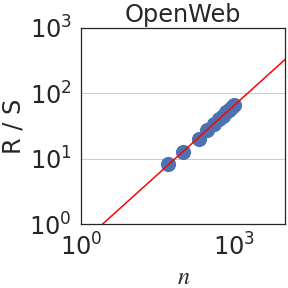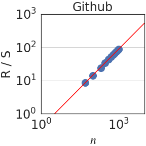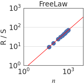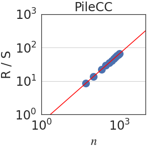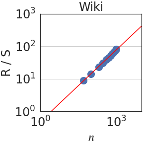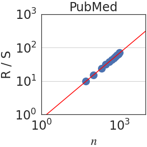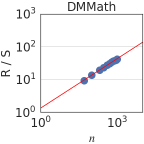Precise Text Transcription * **Top Center:** `ArXiv` * **Y-axis Label:** `R / S` * **X-axis Label:** `n` * **Y-axis Scale:** `10^0`, `10^1`, `10^2`, `10^3` * **X-axis Scale:** `10^0`, `10^3` </details> Figure 3: Rescaled range $R(n)/S(n)$ is plotted against the number of normalized bits $n$ . We observe a power law $R(n)/S(n)\sim n^{\mathrm{H}}$ in all domains. When aggregating all datasets, $\mathrm{H}=0.70± 0.09$ . Besides PaLM2, we also experiment and report on various model sizes of PaLM [12] and decoder-only T5 [54]. Namely, we report results for models: PaLM2 XXS (Gecko), XS (Otter), S (Bison), M, and L (Unicorn); PaLM 8B, 62B, 540B; and decoder-only T5.1.1 at Base (110M), Large (341M), XL (1.2B), and XXL (5B) sizes. For PaLM and PaLM2, we use the checkpoints pretrained in Chowdhery et al., [12] and Anil et al., 2023b [6]. All T5.1.1 decoder baselines, on the other hand, are trained with a casual language modeling objective for 262B tokens of C4 [54]. All experiments are executed on Tensor Processing Units (TPUs). More details on how we train T5.1.1 baselines are in Appendix A. Once $z_{t}$ is computed for a document, we follow standard definitions in constructing the increment process $(x_{t})_{t∈\mathbb{N}}$ by normalizing $z_{t}$ to have a zero-mean and unit variance. Intuitively, fractal parameters are intended to measure a fundamental property of the process (e.g. LRD) that should not be affected by scale, hence the normalization. The integral process $(X_{t})_{t∈\mathbb{N}}$ is calculated based on $(x_{t})_{t∈\mathbb{N}}$ , as described earlier and depicted in Figure 1 (top). Normalizing bits (to have zero mean and unit variance) models language as a random walk. It is a standard approach used extensively in the literature in various contexts, such as in DNA sequences [51, 56, 47, 35, 58]. For analysis, we use The Pile validation split [23], consisting of 22 subdomains such as Wikipedia and GitHub. We restrict analysis to sufficiently-long documents of length $>4K$ tokens and use the first 2K tokens only, to sidestep potential effects of the finite length of documents and the model context. To mitigate noise, only domains with $>1K$ documents are compared; we report results for them separately and their median. We use bootstrapping [17] to estimate the error margin. Notation. We write $f(x)\sim x^{c}$ if $f(x)=x^{c}L(x)$ for some function $L$ that satisfies $L(tx)/L(x)→ 1$ as $x→∞$ for all $t>0$ . Examples of slowly varying functions are constants $L(x)=c$ and $L(x)=\log x$ . When $f(x)\sim x^{c}$ , we abuse terminology slightly by referring to $f(x)$ as a power law. Figure 4: left: Estimates of the self-similarity exponent $\mathrm{S}$ are generally robust to the choice of $\epsilon$ . right: The partial auto-correlation function calculated across domains. DM Mathematics has a much shorter dependence compared to the rest of the domains, in agreement with its Hurst parameter. 2.2 Self-similarity exponent An integral process is said to be self-similar if it exhibits statistical self-similarity. More precisely, $(X_{t})_{t∈\mathbb{N}}$ is self-similar if $(X_{\tau t})_{t∈\mathbb{N}}$ is distributionally equivalent to $(\tau^{S}X_{t})_{t∈\mathbb{N}}$ for some exponent $\mathrm{S}$ . Thus, scaling of time is equivalent to an appropriate scaling of space. We will refer to $\tau$ as the granularity level and to the exponent $\mathrm{S}$ as the self-similarity or Hölder exponent [64]. Many time series in nature exhibit self-similar structures, such as human blood pressure and heart rate [27]. One approach for calculating $\mathrm{S}$ is as follows. Fix $\epsilon\ll 1$ and denote the $\tau$ -increments by $(X_{t+\tau}-X_{t})_{t∈\mathbb{N}}$ . These would correspond, for instance, to the number of bits used for clauses, sentences, paragraphs and longer texts as $\tau$ increases. In terms of the increment process $(x_{t})_{t∈\mathbb{N}}$ , this corresponds to aggregating increments into “bursts”. Let $p_{\epsilon}(\tau)$ be the probability mass of the event $\{|X_{t+\tau}-X_{t}|≤\epsilon\}_{t∈\mathbb{N}}$ . Then, $\mathrm{S}$ can be estimated by fitting a power law relation $p_{\epsilon}(\tau)\sim\tau^{-S}$ [64]. Generally, $\mathrm{S}$ is robust to the choice of $\epsilon∈[10^{-3},10^{-2}]$ as shown in Figure 4 (left) so we fix it to $\epsilon=5× 10^{-3}$ . Figure 2 plots the probability $p_{\epsilon}(\tau)$ against $\tau$ using PaLM2-L. We indeed observe a power law relation; i.e. linear in a log-log scale, with a median self-similarity exponent of $\mathrm{S}=0.59± 0.08$ . Section 3 shows that the median $\mathrm{S}$ is robust to the choice of the LLM. 2.3 Hurst parameter The Hurst parameter $\mathrm{H}∈[0,1]$ quantifies the degree of predictability or dependence over time [31]. It is calculated using the so-called rescaled-range (R/S) analysis. Let $(x_{t})_{t∈\mathbb{N}}$ be an increment process. For each $n∈\mathbb{N}$ , write $y_{t}=x_{t}-\frac{1}{t}\sum_{k=0}^{t}x_{k}$ and $Y_{t}=\sum_{k=0}^{t}y_{t}$ . The range and scale are defined, respectively, as $R(n)=\max_{t≤ n}Y_{t}-\min_{t≤ n}Y_{t}$ and $S(n)=\sigma\left(\{x_{k}\}_{k≤ n}\right)$ , where $\sigma$ is the standard deviation. Then, the Hurst parameter $\mathrm{H}$ is estimated by fitting a power law relation $R(n)/S(n)\sim n^{\mathrm{H}}$ . As stated earlier, for completely random processes, such as a simple Brownian motion, it can be shown that $\mathrm{H}=1/2$ . In addition, $H>1/2$ implies dependence over time [16, 65, 8]. Writing $\rho_{n}=\mathbb{E}[(x_{t+n}x_{t}]$ for the autocovariance function of the increment process $(x_{t})_{t∈\mathbb{N}}$ , the Hurst parameter satisfies $\mathrm{H}=1-\beta/2$ when $\rho_{n}\sim n^{-\beta}$ as $n→∞$ [26, 16]. Since in self-similar processes, $\mathrm{H}>1/2$ implies long-range dependence (LRD), LRD is equivalent to the condition that the autocovariances are not summable. In terms of the integral process, it can be shown that [57]: $\lim_{n→∞}\frac{\mathrm{Var}(X_{n})}{n}=1+2\sum_{i=1}^{∞}\rho_{i}$ . Hence, if $\mathrm{H}<1/2$ , the auto-covariances are summable and $\mathrm{Var}(X_{n})$ grows, at most, linearly fast on $n$ . On the other hand, if the process has LRD, $\mathrm{Var}(X_{n})$ grows superlinearly on $n$ . In particular, using the Euler-Maclaurin summation formula [7, 2], one obtains $\mathrm{Var}(X_{n})\sim n^{2H}$ if $H>1/2$ . Figure 3 plots the rescaled range $R(n)/S(n)$ against $n$ . We observe a power law relation with a median Hurst parameter of $\mathrm{H}=0.70± 0.09$ . Table 1: A comparison of the fractal parameters across 8 different domains with $>1000$ documents each in The Pile benchmark (see Section 2.1 for selection criteria). DM-Mathematics is markedly different because each document consists of questions, with no LRD. | $\mathrm{S}$ $\mathrm{H}$ $\mathrm{J}$ | $0.53±.05$ $0.68±.01$ $0.46±.01$ | $0.60±.05$ $0.79±.01$ $0.49±.00$ | $0.61±.05$ $0.68±.00$ $0.49±.00$ | $0.56±.03$ $0.70±.00$ $0.50±.00$ | $0.62±.02$ $0.74±.01$ $0.52±.00$ | $0.60±.07$ $0.65±.00$ $0.44±.00$ | $0.42±.03$ $0.50±.01$ $0.28±.00$ | $0.70±.03$ $0.72±.01$ $0.49±.00$ | | --- | --- | --- | --- | --- | --- | --- | --- | --- | 2.4 Fractal dimension Broadly speaking, the fractal dimension of an object describes its local complexity. For a geometric object $Z$ , such as the Koch curve, let $\tau$ be a chosen scale (e.g. a short ruler for measuring lengths or a small square for areas). Let $N(\tau)$ be the minimum number of objects of scale $\tau$ that cover $Z$ ; i.e. contain it entirely. Then, the fractal dimension of $Z$ , also called its Hausdorff dimension, is: $\mathrm{D}=-\lim_{\tau→ 0}\left\{\frac{\log N(\tau)}{\log\tau}\right\}$ [53]. For example, a line has a fractal dimension $1$ , in agreement with its topological dimension, because $N(\tau)=C/\tau$ for some constant $C>0$ . By convention, an object is referred to as “fractal” if $\mathrm{D}$ is different from its topological dimension. For example, the fractal dimension of the Koch curve is about 1.26 when its topological dimension is 1. Fractals explain some puzzling observations, such as why estimates of the length of the coast of Britain varied significantly from one study to another, because lengths in fractals are scale-sensitive. Mandelbrot estimated the fractal dimension of the coast of Britain to be 1.25 [42]. The definition above for the fractal dimension $\mathrm{D}$ applies to geometric shapes, but an analogous definition has been introduced for stochastic processes. Let $(x_{t})_{t∈\mathbb{R}}$ be a stationary process with autocovariance $\rho_{n}$ . Then, its fractal dimension $\mathrm{D}$ is determined according to the local behavior of $\rho_{n}$ at the vicinity of $n=0$ , by first normalizing $(x_{t})_{t∈\mathbb{R}}$ to have a zero-mean and a unit variance, and modeling $\rho_{n}$ using a power law $\rho_{n}\sim 1-n^{\alpha}$ as $n→ 0^{+}$ , for $\alpha∈(0,2]$ . Then, the fractal dimension $\mathrm{D}∈[1,\,2]$ of $(x_{t})_{t∈\mathbb{R}}$ is defined by $\mathrm{D}=2-\alpha/2$ [26]. It can be shown that $\mathrm{D}=2-\mathrm{S}$ [26]. For language, this gives a median fractal dimension of $\mathrm{D}=1.41± 0.08$ . 2.5 Joseph effect Finally, we examine another related parameter that is commonly studied in self-similar processes. The motivation behind it comes from the fact that in processes with LRD, one often observes burstiness as shown in Figure 1; i.e. clusters over time in which the process fully resides on one side of the mean, before switching to the other. This is quite unlike random noise, for instance, where measurements are evenly distributed on both sides of the mean. The effect is often referred to as the Joseph effect, named after the biblical story of the seven fat years and seven lean years [65, 45, 64]. A common way to quantify the Joseph effect for integral processes $(X_{t})_{t∈\mathbb{N}}$ is as follows [64]. First, let $\sigma_{\tau}$ be the standard deviation of the $\tau$ -increments $X_{t+\tau}-X_{t}$ . Then, fit a power law relation $\sigma_{\tau}\sim\tau^{\mathrm{J}}$ . The exponent $\mathrm{J}$ here is called the Joseph exponent. In an idealized fractional Brownian motion, both $\mathrm{J}$ and the self-similarity exponent $\mathrm{S}$ coincide. Figure 5 provides the detailed empirical results. Overall, we find that $\mathrm{J}=0.49± 0.08$ . *[Error downloading image: extracted/2402.01825v2/figs/joseph/joseph_exponent_fit_OpenWebText2.png]* *[Error downloading image: extracted/2402.01825v2/figs/joseph/joseph_exponent_fit_Github.png]* *[Error downloading image: extracted/2402.01825v2/figs/joseph/joseph_exponent_fit_FreeLaw.png]* *[Error downloading image: extracted/2402.01825v2/figs/joseph/joseph_exponent_fit_Pile-CC.png]* *[Error downloading image: extracted/2402.01825v2/figs/joseph/joseph_exponent_fit_Wikipediaen.png]* *[Error downloading image: extracted/2402.01825v2/figs/joseph/joseph_exponent_fit_PubMedCentral.png]* *[Error downloading image: extracted/2402.01825v2/figs/joseph/joseph_exponent_fit_DMMathematics.png]* *[Error downloading image: extracted/2402.01825v2/figs/joseph/joseph_exponent_fit_ArXiv.png]* Figure 5: The standard deviation $\sigma$ of the $\tau$ -increments $X_{t+\tau}-X_{t}$ is plotted against the scale $\tau$ . We, again, observe another power law relation $\sigma\sim\tau^{\mathrm{J}}$ , with a Joseph exponent $\mathrm{J}=0.49± 0.08$ . 3 Analysis Comparative Analysis. Table 1 compares fractal parameters across different domains, such as ArXiv, Github and Wikipedia. In general, most domains share similar self-similarity and Hurst exponents with a few exceptions. The first notable exception is DM-Mathematics, which has a Hurst parameter of about 0.5, indicating a lack of LRD. Upon closer inspection, however, a value of $\mathrm{H}=0.5$ is not surprising for DM-Mathematics because its documents consist of independent mathematical questions as shown in Figure 6. In Figure 4 (right), we plot the partial autocorrelation function for each of the 8 domains against time lag (context length). Indeed, we see that DM-Mathematics shows markedly less dependence compared to the other domains. The second notable observation is the relatively larger value of $\mathrm{H}=0.79$ in GitHub, indicating more structure in code. This is in agreement with earlier findings by Kokol and Podgorelec, [35] who estimated LRD in computer languages to be greater than in natural language. In Table 2, we compare the three fractal parameters $\mathrm{S}$ , $\mathrm{H}$ and $\mathrm{J}$ using different families of LLM and different model sizes. Overall, we observe that the parameters are generally robust to the choice of the architecture. Table 2: A comparison of the estimated median fractal parameters by various LLMs over the entire Pile validation split. Estimates are generally robust to the choice of the LLM, but the tiny variations in median $\mathrm{H}$ reflect improvements in the model quality. See Section 3. | 110M Self-similarity exponent $\mathrm{S}$ | 340M | 1B | 5B | 8B | 62B | 540B | XXS | XS | S | M | L | | --- | --- | --- | --- | --- | --- | --- | --- | --- | --- | --- | --- | | $.58^{±.06}$ | $.60^{±.06}$ | $.60^{±.05}$ | $.58^{±.08}$ | $.60^{±.07}$ | $.62^{±.08}$ | $.64^{±.08}$ | $.59^{±.06}$ | $.57^{±.08}$ | $.56^{±.05}$ | $.59^{±.07}$ | $.60^{±.08}$ | | Hurst exponent $\mathrm{H}$ | | | | | | | | | | | | | $.64^{±.08}$ | $.64^{±.08}$ | $.64^{±.09}$ | $.64^{±.08}$ | $.66^{±.07}$ | $.68^{±.07}$ | $.68^{±.07}$ | $.66^{±.07}$ | $.66^{±.07}$ | $.67^{±.08}$ | $.68^{±.09}$ | $.69^{±.09}$ | | Joseph exponent $\mathrm{J}$ | | | | | | | | | | | | | $.44^{±.06}$ | $.44^{±.06}$ | $.44^{±.06}$ | $.44^{±.06}$ | $.47^{±.06}$ | $.47^{±.06}$ | $.48^{±.06}$ | $.47^{±.06}$ | $.47^{±.06}$ | $.48^{±.07}$ | $.48^{±.07}$ | $.49^{±.08}$ | Figure 6: Two examples of documents from the DM-Mathematics subset of The Pile benchmark [23]. Each document comprises of multiple independent questions. The lack of LRD in this data is reflected in its Hurst parameter of $\mathrm{H}=0.50± 0.01$ | Col1 | | --- | | Document I: What is the square root of 211269 to the nearest integer? 460. What is the square root of 645374 to the nearest integer? 803... | | Document II: Suppose 5*l = r - 35, -2*r + 5*l - 15 = -70. Is r a multiple of 4? True. Suppose 2*l + 11 - 1 = 0. Does 15 divide (-2)/l - 118/(-5)? False... | Downstream Performance. By definition, fractal parameters are calculated on the sequence of negative log-probability scores after normalizing them to zero-mean and unit variance. Hence, they may offer an assessment of downstream performance that improves upon using a perplexity-based metric like bits-per-byte (BPB) alone. To test this hypothesis, we evaluate the 12 models in Table 2 on challenging downstream zero- and few-shot benchmarks focusing on language understanding and reasoning. We include results for 0-shot (0S) and 3-shot (3S) evaluation for BIG-Bench Hard tasks [62, 63] reporting both direct and chain-of-thought (CoT) prompting results following Chung et al., [13]. In addition we report 0-shot and 5-shot (5S) MMLU [30], and 8-shot (8S) GSM8K [14] with CoT. Raw accuracy is reported for all tasks. BBH and MMLU scores are averaged across all 21 tasks and 57 subjects, respectively. All prompt templates for our evaluation are taken from Chung et al., [13], Longpre et al., [41], which we refer the reader to for more details. We prompt all models using a 2048 context length. See Table 8 of Appendix C for the full results. The first (surprising) observation is that the median Hurst parameter is itself strongly correlated with the BPB scores with an absolute Pearson correlation coefficient of 0.83, even though the Hurst exponent is calculated after normalizing all token losses to zero-mean and unit variance! Informally, this implies that second-order statistics on the sequence of token losses of a particular model can predict its mean! Self-similarity exponent, by contrast, has an absolute correlation of 0.23 with BPB. Figure 7 displays downstream performance against both the median Hurst exponent and the median BPB score, where median values are calculated on the 8 domains in The Pile benchmark listed in Table 1. In general, both the BPB score and the median Hurst are good predictors of downstream performance. However, we observe that improvements in BPB alone without impacting the median Hurst exponent do not directly translate into improvements downstream. This is verified quantitatively in Table 3 (middle), which reports the adjusted $R^{2}$ values – the proportion of variance in each downstream metric that can be predicted using BPB, $\mathrm{H}$ , or by combining them together into $\mathrm{H}_{B}=1/\mathrm{BPB}+\mathrm{H}$ , with BPB replaced with its reciprocal so that higher values are better. We observe that $\mathrm{H}_{B}$ yields indeed a stronger predictor of downstream performance. Hence, while $\mathrm{H}$ and BPB are correlated, combining them yields a better predictor, so each of $\mathrm{H}$ and BPB conveys useful information not captured by the other metric. See Appendix C for similar analysis using the exponents $\mathrm{S}$ and $\mathrm{J}$ . Table 3: middle three columns show the adjusted $R^{2}$ : the proportion of variation in downstream performance (row) predictable by a linear function of the input (column). Median Hurst ( $\mathrm{H}$ ) and (especially) the combined metric $\mathrm{H}_{B}$ predict downstream performance better than BPB alone. $\mathrm{S}$ and $\mathrm{J}$ do not give any improvement (see Appendix C). right: the downstream performance for three decoder-only T5.1.1. models pretrained on 100B tokens with 2K, 4K, or 8K context lengths. | Benchmark 0S BBH Direct 0S MMLU | BPB 0.785 0.653 | $\mathrm{H}$ 0.841 0.831 | $\mathrm{H}_{B}$ 0.883 0.825 | 2K 0 1.81 25.73 | 4K 0 1.68 26.04 | 8K 0 1.76 25.81 | | --- | --- | --- | --- | --- | --- | --- | | 0S BBH+MMLU | 0.685 | 0.849 | 0.852 | 13.39 | 13.49 | 13.42 | | 3S BBH Direct | 0.767 | 0.895 | 0.926 | 21.35 | 24.76 | 23.14 | | 3S BBH CoT | 0.881 | 0.892 | 0.979 | 16.87 | 12.21 | 0 7.14 | | 5S MMLU | 0.660 | 0.853 | 0.832 | 26.57 | 26.69 | 27.07 | | 8S GSM8K CoT | 0.654 | 0.867 | 0.851 | 0 1.06 | 0 1.21 | 0 1.74 | | FS BBH+MMLU+GSM8K | 0.717 | 0.890 | 0.891 | 15.58 | 15.46 | 14.65 | Figure 7: Downstream metric, indicated by bubble size where larger is better, is plotted vs. the median Hurst and the median BPB for all 12 language models. Context Length at Training Time (Negative Result). Finally, we present a negative result. Self-similarity and LRD point to an intriguing possibility: the importance of training the model with extensive contexts in order to capture the fractal-nature of language, which may elevate the model’s capabilities regardless of the context length needed during inference. To test this hypothesis, we pretrain three decoder-only T5.1.1 models with 1B parameters on SlimPajama-627B [61] for up to 100B tokens using three context lengths: 2K, 4K and 8K, all observing the same number of tokens per batch. We use SlimPajama-627B instead of C4 because most documents in C4 are short ( $≈ 94\%$ of them are $<2K$ tokens in length). Refer to Appendix A for details. These models are, then, evaluated on the same downstream benchmarks listed in Figure 7. As shown in Table 3 (right) however, we do not observe any improvements in performance with context length in this particular setup. 4 Related Works and Directions for Future Research The statistical attributes of human language have long piqued scholarly curiosity, such as One example is Zipf’s law, which Shannon leveraged to estimate the entropy of English to be around 1 bit per letter [59], but his calculation did not consider second-order statistics. More recently, Eftekhari, [18] proposed a refinement to Zipf’s law, suggesting its application to letters rather than words. Another related result is Heap’s law, which states that the number of unique words is a power law function of the document’s length [29]. However, both Zipf’s and Heap’s laws are invariant to the semantic ordering of text, so they do not capture important aspects, such as long-range dependence (LRD) [48]. In terms of self-similarity in language, the Menzerath-Altmann law stipulates a self-similar behavior in the following sense: when the size of a language construct increases, the size of its constituents decreases, and this happens at all scales [48, 4]. In Ausloos, [9], the authors model texts as a time series by replacing a word with its length. After that, they study the fractal behavior of language. However, as mentioned in [22], replacing a word with its length is invalid because it is not translation-independent (i.e. one could map every word to an arbitrary token, including tokens of equal length). In our work, we model language as a series of bits calculated from conditional entropies, reflecting the intrinsic structure of the language itself, inspired by findings in linguistics such as [28, 22, 40]. In Najafi and Darooneh, [48], the authors define a fractal dimension for each word. Informally, they examine the recurrence of a single, predetermined word as a binary series, similar to the approach used in Altmann et al., [3]. However, this only applies to individual words and cannot model higher-level clauses. For instance, it does not distinguish between “time” in the phrase “once upon a time” and “time” in “space and time.” Kokol and Podgorelec, [35] estimate LRD in natural language, and suggest that its LRD is close to that of pure noise! They conjecture this was due to their use of ASCII encoding. In computer languages, they observe LRD and suggest it is because they are formal. Besides the above concerns in prior studies that examined the self-similar structure in language, another concern is that they sometimes give extremely large values of the fractal dimension, sometimes exceeding 10 [4]! Such values are difficult to interpret because the fractal dimension $\mathrm{D}$ should fall in $\mathrm{D}∈[1,2]$ for time series. We do not observe such issues in our analysis. In our case, $\mathrm{D}=1.41± 0.08$ . Limitations and Future Research. Our analysis is currently limited to the English language so it may not apply to other languages that differ significantly. For instance, some languages such as Pirahã (spoken in the Amazon) do not have a recursive structure like most languages do [20]. We also do not model the semantic or lexical form of language. While our information-theoretic approach is well-founded and captures the intrinsic complexity of language, it does not account for the semantic nuances that contribute to meaning. Thirdly, self-similarity may explain why parameter sharing, such as in ALBERT [37], can be successful but exploiting self-similarity more directly in LLMs could lead to further optimizations. Exploring these aspects are promising directions for future research. 5 Concluding Remarks In this work, we highlight intriguing insights into the underlying fractal structure of language and how it may be interconnected with the remarkable capabilities of LLMs. Our formalism quantifies properties of language that may have been suspected, but not previously formally shown. In particular, the need in LLMs to balance between short- and long-term contexts is reflected in the self-similar structure of language, while long-range dependence is quantifiable using the Hurst parameter. For instance, the absence of LRD in DM-Mathematics is reflected in its Hurst parameter of $\mathrm{H}≈ 0.5$ . Interestingly, the estimated median Hurst value of $\mathrm{H}=0.70± 0.09$ in language reflects an intriguing balance between predictability and noise that is similar to many other phenomena, and combining both $\mathrm{H}$ with BPB together yields a stronger predictor of downstream performance. We carry out an extensive comparative analysis across different domains and model architectures, revealing that fractal parameters are generally robust. We hope that future research can further probe into these fractal properties, unearthing deeper understandings of the relation between intelligence and language. Acknowledgement The authors would like to thank Justin Gilmer and Olivier Bousquet for their feedback on earlier drafts of this manuscript, and both Google Deepmind and Google Research teams at large for the insightful discussions and providing a supportive research environment. References - Abry et al., [1995] Abry, P., Gonçalvés, P., and Flandrin, P. (1995). Wavelets, spectrum analysis and 1/f processes. Wavelets and statistics, pages 15–29. - Alabdulmohsin, [2018] Alabdulmohsin, I. M. (2018). Summability calculus: A comprehensive theory of fractional finite sums. Springer. - Altmann et al., [2012] Altmann, E. G., Cristadoro, G., and Esposti, M. D. (2012). On the origin of long-range correlations in texts. Proceedings of the National Academy of Sciences, 109(29):11582–11587. - Andres, [2009] Andres, J. (2009). On de Saussure’s principle of linearity and visualization of language structures. Glottotheory, 2(2):1–14. - [5] Anil, R., Borgeaud, S., Wu, Y., Alayrac, J.-B., Yu, J., Soricut, R., Schalkwyk, J., Dai, A. M., Hauth, A., Millican, K., Silver, D., Petrov, S., Johnson, M., Antonoglou, I., Schrittwieser, J., Glaese, A., Chen, J., Pitler, E., et al. (2023a). Gemini: A family of highly capable multimodal models. arXiv:2312.11805v1 [cs.CL]. - [6] Anil, R., Dai, A. M., Firat, O., Johnson, M., Lepikhin, D., Passos, A., Shakeri, S., Taropa, E., Bailey, P., Chen, Z., Chu, E., Clark, J. H., Shafey, L. E., Huang, Y., Meier-Hellstern, K., Mishra, G., Moreira, E., Omernick, M., Robinson, K., Ruder, S., Tay, Y., Xiao, K., Xu, Y., Zhang, Y., Abrego, G. H., Ahn, J., Austin, J., Barham, P., Botha, J., Bradbury, J., Brahma, S., Brooks, K., Catasta, M., Cheng, Y., Cherry, C., Choquette-Choo, C. A., Chowdhery, A., Crepy, C., Dave, S., Dehghani, M., Dev, S., Devlin, J., Díaz, M., Du, N., Dyer, E., Feinberg, V., Feng, F., Fienber, V., Freitag, M., Garcia, X., Gehrmann, S., Gonzalez, L., Gur-Ari, G., Hand, S., Hashemi, H., Hou, L., Howland, J., Hu, A., Hui, J., Hurwitz, J., Isard, M., Ittycheriah, A., Jagielski, M., Jia, W., Kenealy, K., Krikun, M., Kudugunta, S., Lan, C., Lee, K., Lee, B., Li, E., Li, M., Li, W., Li, Y., Li, J., Lim, H., Lin, H., Liu, Z., Liu, F., Maggioni, M., Mahendru, A., Maynez, J., Misra, V., Moussalem, M., Nado, Z., Nham, J., Ni, E., Nystrom, A., Parrish, A., Pellat, M., Polacek, M., Polozov, A., Pope, R., Qiao, S., Reif, E., Richter, B., Riley, P., Ros, A. C., Roy, A., Saeta, B., Samuel, R., Shelby, R., Slone, A., Smilkov, D., So, D. R., Sohn, D., Tokumine, S., Valter, D., Vasudevan, V., Vodrahalli, K., Wang, X., Wang, P., Wang, Z., Wang, T., Wieting, J., Wu, Y., Xu, K., Xu, Y., Xue, L., Yin, P., Yu, J., Zhang, Q., Zheng, S., Zheng, C., Zhou, W., Zhou, D., Petrov, S., and Wu, Y. (2023b). PaLM 2 technical report. arXiv:2305.10403v3 [cs.CL]. - Apostol, [1999] Apostol, T. M. (1999). An elementary view of Euler’s summation formula. The American Mathematical Monthly, 106(5):409–418. - Aref, [1998] Aref, S. (1998). Hurst phenomenon and fractal dimensions in long-term yield data. In Conference on Applied Statistics in Agriculture. - Ausloos, [2012] Ausloos, M. (2012). Generalized Hurst exponent and multifractal function of original and translated texts mapped into frequency and length time series. Physical Review E, 86(3):031108. - Bradbury et al., [2018] Bradbury, J., Frostig, R., Hawkins, P., Johnson, M. J., Leary, C., Maclaurin, D., Necula, G., Paszke, A., VanderPlas, J., Wanderman-Milne, S., and Zhang, Q. (2018). JAX: composable transformations of Python+NumPy programs. - Bubeck et al., [2023] Bubeck, S., Chandrasekaran, V., Eldan, R., Gehrke, J., Horvitz, E., Kamar, E., Lee, P., Lee, Y. T., Li, Y., Lundberg, S., Nori, H., Palangi, H., Ribeiro, M. T., and Zhang, Y. (2023). Sparks of artificial general intelligence: Early experiments with GPT-4. - Chowdhery et al., [2022] Chowdhery, A., Narang, S., Devlin, J., Bosma, M., Mishra, G., Roberts, A., Barham, P., Chung, H. W., Sutton, C., Gehrmann, S., et al. (2022). PaLM: Scaling language modeling with pathways. arXiv preprint arXiv:2204.02311. - Chung et al., [2022] Chung, H. W., Hou, Le and, L. S., Zoph, B., Tay, Y., Fedus, W., and et al. (2022). Scaling instruction-finetuned language models. arXiv:2210.11416v5 [cs.LG]. - Cobbe et al., [2021] Cobbe, K., Kosaraju, V., Bavarian, M., Hilton, J., Nakano, R., Hesse, C., and Schulman, J. (2021). Training verifiers to solve math word problems. arXiv:2110.14168v2 [cs.LG]. - Cover, [1999] Cover, T. M. (1999). Elements of information theory. John Wiley & Sons. - Crovella and Bestavros, [1995] Crovella, M. E. and Bestavros, A. (1995). Explaining world wide web traffic self-similarity. Technical report, Boston University Computer Science Department. - Efron and Tibshirani, [1994] Efron, B. and Tibshirani, R. J. (1994). An introduction to the bootstrap. CRC press. - Eftekhari, [2006] Eftekhari, A. (2006). Fractal geometry of texts: An initial application to the works of Shakespeare. Journal of Quantitative Linguistics, 13(2-3):177–193. - Embrechts and Maejima, [2000] Embrechts, P. and Maejima, M. (2000). An introduction to the theory of self-similar stochastic processes. International journal of modern physics B, 14(12n13):1399–1420. - Everett, [2005] Everett, D. (2005). Cultural constraints on grammar and cognition in pirahã: Another look at the design features of human language. Current anthropology, 46(4):621–646. - Feller, [1951] Feller, W. (1951). The Asymptotic Distribution of the Range of Sums of Independent Random Variables. The Annals of Mathematical Statistics, 22(3):427 – 432. - Futrell and Hahn, [2022] Futrell, R. and Hahn, M. (2022). Information theory as a bridge between language function and language form. Frontiers in Communication, 7:657725. - Gao et al., [2020] Gao, L., Biderman, S., Black, S., Golding, L., Hoppe, T., Foster, C., Phang, J., He, H., Thite, A., Nabeshima, N., Presser, S., and Leahy, C. (2020). The Pile: An 800GB dataset of diverse text for language modeling. arXiv:2101.00027v1 [cs.CL]. - Geweke and Porter-Hudak, [1983] Geweke, J. and Porter-Hudak, S. (1983). The estimation and application of long memory time series models. Journal of time series analysis, 4(4):221–238. - Gibson et al., [2019] Gibson, E., Futrell, R., Piantadosi, S. P., Dautriche, I., Mahowald, K., Bergen, L., and Levy, R. (2019). How efficiency shapes human language. Trends in cognitive sciences, 23(5):389–407. - Gneiting and Schlather, [2004] Gneiting, T. and Schlather, M. (2004). Stochastic models that separate fractal dimension and the Hurst effect. SIAM Review, 46(2):269–282. - Goldberger et al., [2002] Goldberger, A. L., Amaral, L. A., Hausdorff, J. M., Ivanov, P. C., Peng, C.-K., and Stanley, H. E. (2002). Fractal dynamics in physiology: alterations with disease and aging. Proceedings of the national academy of sciences, 99(suppl_1):2466–2472. - Hale, [2001] Hale, J. (2001). A probabilistic earley parser as a psycholinguistic model. In Second meeting of the north american chapter of the association for computational linguistics. - Heaps, [1978] Heaps, H. S. (1978). Information retrieval, computational and theoretical aspects. Academic Press. - Hendrycks et al., [2020] Hendrycks, D., Burns, C., Basart, S., Zou, A., Mazeika, M., Song, D., and Steinhardt, J. (2020). Measuring massive multitask language understanding. arXiv preprint arXiv:2009.03300. - Hurst, [1951] Hurst, H. E. (1951). Long-term storage capacity of reservoirs. Transactions of the American society of civil engineers, 116(1):770–799. - Jouppi et al., [2020] Jouppi, N. P., Yoon, D. H., Kurian, G., Li, S., Patil, N., Laudon, J., Young, C., and Patterson, D. (2020). A domain-specific supercomputer for training deep neural networks. Communications of the ACM, 63(7):67–78. - Kadavath et al., [2022] Kadavath, S., Conerly, T., Askell, A., Henighan, T., Drain, D., Perez, E., Schiefer, N., Hatfield-Dodds, Z., DasSarma, N., Tran-Johnson, E., et al. (2022). Language models (mostly) know what they know. arXiv preprint arXiv:2207.05221. - Kidd and Hayden, [2015] Kidd, C. and Hayden, B. Y. (2015). The psychology and neuroscience of curiosity. Neuron, 88(3):449–460. - Kokol and Podgorelec, [2000] Kokol, P. and Podgorelec, V. (2000). Complexity and human writings. Complexity, 7:1–6. - Kolmogorov, [1940] Kolmogorov, A. N. (1940). Wienersche spiralen und einige andere interessante kurven in hilbertscen raum, cr (doklady). Acad. Sci. URSS (NS), 26:115–118. - Lan et al., [2019] Lan, Z., Chen, M., Goodman, S., Gimpel, K., Sharma, P., and Soricut, R. (2019). ALBERT: A lite BERT for self-supervised learning of language representations. arXiv preprint arXiv:1909.11942. - Leland et al., [1994] Leland, W. E., Taqqu, M. S., Willinger, W., and Wilson, D. V. (1994). On the self-similar nature of Ethernet traffic. IEEE/ACM Transactions on networking, 2(1):1–15. - Leland and Wilson, [1991] Leland, W. E. and Wilson, D. V. (1991). High time-resolution measurement and analysis of LAN traffic: Implications for LAN interconnection. In IEEE INFCOM. - Levy, [2008] Levy, R. (2008). Expectation-based syntactic comprehension. Cognition, 106(3):1126–1177. - Longpre et al., [2023] Longpre, S., Hou, L., Vu, T., Webson, A., Chung, H. W., Tay, Y., Zhou, D., Le, Q. V., Zoph, B., Wei, J., and Roberts, A. (2023). The flan collection: designing data and methods for effective instruction tuning. In Proceedings of the 40th International Conference on Machine Learning, ICML’23. JMLR.org. - Mandelbrot, [1967] Mandelbrot, B. (1967). How long is the coast of Britain? Statistical self-similarity and fractional dimension. science, 156(3775):636–638. - Mandelbrot, [2002] Mandelbrot, B. (2002). Gaussian self-affinity and fractals: globality, the earth, 1/f noise, and R/S. Springer Science and Business Media. - Mandelbrot, [1982] Mandelbrot, B. B. (1982). The fractal geometry of nature. WH freeman New York. - Mandelbrot and Wallis, [1968] Mandelbrot, B. B. and Wallis, J. R. (1968). Noah, Joseph, and operational hydrology. Water resources research, 4(5):909–918. - Mollica et al., [2021] Mollica, F., Bacon, G., Zaslavsky, N., Xu, Y., Regier, T., and Kemp, C. (2021). The forms and meanings of grammatical markers support efficient communication. Proceedings of the National Academy of Sciences, 118(49):e2025993118. - Montemurro and Pury, [2002] Montemurro, M. A. and Pury, P. A. (2002). Long-range fractal correlations in literary corpora. Fractals, 10(04):451–461. - Najafi and Darooneh, [2015] Najafi, E. and Darooneh, A. H. (2015). The fractal patterns of words in a text: a method for automatic keyword extraction. PloS one, 10(6):e0130617. - OpenAI, [2023] OpenAI (2023). GPT-4 technical report. arXiv:2303.08774v4 [cs.CL]. - Paxson and Floyd, [1995] Paxson, V. and Floyd, S. (1995). Wide area traffic: the failure of Poisson modeling. IEEE/ACM Transactions on networking, 3(3):226–244. - Peng et al., [1992] Peng, C.-K., Buldyrev, S. V., Goldberger, A. L., Havlin, S., Sciortino, F., Simons, M., and Stanley, H. E. (1992). Long-range correlations in nucleotide sequences. Nature, 356(6365):168–170. - Perfors et al., [2010] Perfors, A., Tenenbaum, J., Gibson, E., and Regier, T. (2010). How recursive is language? a bayesian exploration. Recursion and human language, pages 159–175. - Pilgrim and Taylor, [2018] Pilgrim, I. and Taylor, R. P. (2018). Fractal analysis of time-series data sets: Methods and challenges. In Ouadfeul, S.-A., editor, Fractal Analysis, chapter 2. IntechOpen, Rijeka. - Raffel et al., [2019] Raffel, C., Shazeer, N., Roberts, A., Lee, K., Narang, S., Matena, M., Zhou, Y., Li, W., and Liu, P. J. (2019). Exploring the limits of transfer learning with a unified text-to-text transformer. arXiv:1910.10683v4 [cs.LG]. - Roberts et al., [2022] Roberts, A., Chung, H. W., Levskaya, A., Mishra, G., Bradbury, J., Andor, D., Narang, S., Lester, B., Gaffney, C., Mohiuddin, A., Hawthorne, C., Lewkowycz, A., Salcianu, A., van Zee, M., Austin, J., Goodman, S., Soares, L. B., Hu, H., Tsvyashchenko, S., Chowdhery, A., Bastings, J., Bulian, J., Garcia, X., Ni, J., Chen, A., Kenealy, K., Clark, J. H., Lee, S., Garrette, D., Lee-Thorp, J., Raffel, C., Shazeer, N., Ritter, M., Bosma, M., Passos, A., Maitin-Shepard, J., Fiedel, N., Omernick, M., Saeta, B., Sepassi, R., Spiridonov, A., Newlan, J., and Gesmundo, A. (2022). Scaling up models and data with t5x and seqio. - Roche et al., [2003] Roche, S., Bicout, D., Maciá, E., and Kats, E. (2003). Long range correlations in DNA: scaling properties and charge transfer efficiency. Physical review letters, 91(22):228101. - Samorodnitsky, [2006] Samorodnitsky, G. (2006). Long memory and self-similar processes. In Annales de la Faculté des sciences de Toulouse: Mathématiques, volume 15, pages 107–123. - Schenkel et al., [1993] Schenkel, A., Zhang, J., and Zhang, Y.-C. (1993). Long range correlation in human writings. Fractals, 1(01):47–57. - Shannon, [1951] Shannon, C. E. (1951). Prediction and entropy of printed English. Bell system technical journal, 30(1):50–64. - Shazeer and Stern, [2018] Shazeer, N. and Stern, M. (2018). Adafactor: Adaptive learning rates with sublinear memory cost. In International Conference on Machine Learning, pages 4596–4604. PMLR. - Soboleva et al., [2023] Soboleva, D., Al-Khateeb, F., Myers, R., Steeves, J. R., Hestness, J., and Dey, N. (2023). SlimPajama: A 627B token cleaned and deduplicated version of RedPajama. - Srivastava et al., [2022] Srivastava, A., Rastogi, A., Rao, A., Shoeb, A. A. M., Abid, A., Fisch, A., Brown, A. R., Santoro, A., Gupta, A., Garriga-Alonso, A., et al. (2022). Beyond the imitation game: Quantifying and extrapolating the capabilities of language models. arXiv preprint arXiv:2206.04615. - Suzgun et al., [2022] Suzgun, M., Scales, N., Scharli, N., Gehrmann, S., Tay, Y., Chung, H. W., Chowdhery, A., Le, Q. V., Chi, E. H., Zhou, D., and Wei, J. (2022). Challenging BIG-Bench tasks and whether chain-of-thought can solve them. arXiv:2210.09261v1 [cs.CL]. - Watkins, [2019] Watkins, N. (2019). Mandelbrot’s stochastic time series models. Earth and Space Science, 6(11):2044–2056. - Willinger et al., [1995] Willinger, W., Taqqu, M. S., Leland, W. E., and Wilson, D. V. (1995). Self-similarity in high-speed packet traffic: analysis and modeling of Ethernet traffic measurements. Statistical science, pages 67–85. - Willinger et al., [1997] Willinger, W., Taqqu, M. S., Sherman, R., and Wilson, D. V. (1997). Self-similarity through high-variability: statistical analysis of Ethernet LAN traffic at the source level. IEEE/ACM Transactions on networking, 5(1):71–86. Appendix A Experiment Details All of our experiments are conducted in JAX/Flax [10] using the open source T5X framework [55]. T5 baselines in Table 2 and 3 are pretrained from scratch using the open source T5.1.1 decoder-only architecture from the T5X library. https://github.com/google-research/t5x/tree/main/t5x/examples/decoder_only/models. We pretrain using a causal language modeling objective over the C4 corpus with the default T5 vocabulary as per Raffel et al., [54]. Training is done for 500k steps with a sequence length of 1024 and batch size of 512, resulting in a total of 262B tokens seen during pretraining. We optimize our model with the Adafactor [60] optimizer with an inverse square root learning rate schedule, 1k warmup steps, and an initial learning rate of 1e-2. Models are trained using 256 TPUv5e chips [32]. T5 context length ablation experiments in Table 3 are trained with the same pretraining objective but over the SlimPajama-627B corpus [61] and using a modified version of the T5 vocabulary that preserves whitespace and introduces byte-fallback for out of vocabulary tokens. This is similar to Chowdhery et al., [12], but preserving the original T5 vocabulary. Models with sequence lengths 2048, 4096, 8192 are trained with batch sizes of 512, 256, and 128 respectively to preserve the number of tokens seen per batch and overall training steps. We train all models for 100k steps, using the same learning rate schedule described above. Hence, all models observe 100B tokens. Appendix B Full Results In this section, we provide the full list of parameters calculated for each combination of LLM and domain. We use bootstrapping [17] to estimate the error margin. Table 4: Log-perplexity (NLL) scores evaluated on the first 2048 tokens, after trimming the first 100 tokens, of documents belonging to each of the shown domains. Only documents with a minimum length of 4K tokens are used. | Model T5-Decoder-110M T5-Decoder-340M | OpenWebText2 2.89 2.60 | Github 1.82 1.56 | FreeLaw 2.45 2.14 | Pile-CC 2.88 2.62 | Wikipedia 2.80 2.52 | PubMed 2.36 2.08 | Mathematics 2.28 2.10 | ArXiv 2.70 2.42 | | --- | --- | --- | --- | --- | --- | --- | --- | --- | | T5-Decoder-1B | 2.38 | 1.37 | 1.91 | 2.41 | 2.29 | 1.88 | 2.00 | 2.19 | | T5-Decoder-5B | 2.19 | 1.22 | 1.73 | 2.25 | 2.11 | 1.73 | 1.91 | 2.01 | | PaLM1-8B | 2.26 | 0.79 | 1.66 | 2.36 | 2.08 | 1.89 | 1.40 | 2.08 | | PaLM1-62B | 2.02 | 0.62 | 1.44 | 2.14 | 1.80 | 1.68 | 1.30 | 1.83 | | PaLM1-540B | 1.88 | 0.54 | 1.33 | 2.01 | 1.58 | 1.57 | 1.25 | 1.68 | | PaLM2-XXS | 2.37 | 0.87 | 1.77 | 2.46 | 2.17 | 1.96 | 1.38 | 1.96 | | PaLM2-XS | 2.12 | 0.73 | 1.53 | 2.22 | 1.92 | 1.72 | 1.27 | 1.72 | | PaLM2-S | 1.95 | 0.60 | 1.37 | 2.06 | 1.71 | 1.57 | 1.19 | 1.55 | | PaLM2-M | 1.88 | 0.56 | 1.31 | 1.99 | 1.59 | 1.51 | 1.12 | 1.48 | | PaLM2-L | 1.75 | 0.46 | 1.23 | 1.88 | 1.22 | 1.43 | 1.08 | 1.36 | Table 5: Self-similarity exponent $\mathrm{S}$ evaluated on the first 2048 tokens, after trimming the first 100 tokens, of documents belonging to each of the shown domains. Only documents with a minimum length of 4K tokens are used. | Model T5-Decoder-110M T5-Decoder-340M | OpenWebText2 $0.58± 0.04$ $0.52± 0.03$ | Github $0.67± 0.03$ $0.59± 0.05$ | FreeLaw $0.51± 0.02$ $0.63± 0.04$ | Pile-CC $0.54± 0.07$ $0.58± 0.04$ | Wikipedia $0.59± 0.04$ $0.61± 0.03$ | PubMed $0.59± 0.03$ $0.61± 0.03$ | Mathematics $0.51± 0.04$ $0.48± 0.04$ | ArXiv $0.58± 0.05$ $0.61± 0.05$ | | --- | --- | --- | --- | --- | --- | --- | --- | --- | | T5-Decoder-1B | $0.54± 0.01$ | $0.66± 0.11$ | $0.61± 0.06$ | $0.57± 0.06$ | $0.59± 0.05$ | $0.60± 0.02$ | $0.50± 0.03$ | $0.63± 0.02$ | | T5-Decoder-5B | $0.51± 0.04$ | $0.70± 0.04$ | $0.60± 0.04$ | $0.58± 0.02$ | $0.58± 0.03$ | $0.57± 0.02$ | $0.45± 0.02$ | $0.67± 0.05$ | | PaLM1-8B | $0.56± 0.03$ | $0.67± 0.05$ | $0.63± 0.05$ | $0.58± 0.01$ | $0.55± 0.04$ | $0.62± 0.03$ | $0.50± 0.03$ | $0.68± 0.07$ | | PaLM1-62B | $0.49± 0.03$ | $0.65± 0.09$ | $0.63± 0.09$ | $0.57± 0.03$ | $0.63± 0.05$ | $0.61± 0.04$ | $0.48± 0.05$ | $0.68± 0.03$ | | PaLM1-540B | $0.51± 0.04$ | $0.68± 0.09$ | $0.64± 0.05$ | $0.58± 0.04$ | $0.67± 0.03$ | $0.64± 0.08$ | $0.48± 0.03$ | $0.65± 0.04$ | | PaLM2-XXS | $0.53± 0.02$ | $0.61± 0.05$ | $0.58± 0.04$ | $0.60± 0.04$ | $0.57± 0.05$ | $0.61± 0.03$ | $0.52± 0.02$ | $0.70± 0.04$ | | PaLM2-XS | $0.54± 0.04$ | $0.57± 0.06$ | $0.58± 0.03$ | $0.56± 0.04$ | $0.60± 0.04$ | $0.57± 0.06$ | $0.45± 0.02$ | $0.73± 0.06$ | | PaLM2-S | $0.55± 0.02$ | $0.55± 0.15$ | $0.59± 0.02$ | $0.54± 0.08$ | $0.65± 0.04$ | $0.58± 0.05$ | $0.49± 0.04$ | $0.61± 0.03$ | | PaLM2-M | $0.58± 0.02$ | $0.62± 0.06$ | $0.59± 0.04$ | $0.60± 0.05$ | $0.70± 0.03$ | $0.56± 0.04$ | $0.46± 0.04$ | $0.62± 0.05$ | | PaLM2-L | $0.53± 0.05$ | $0.60± 0.05$ | $0.61± 0.05$ | $0.56± 0.03$ | $0.62± 0.02$ | $0.60± 0.07$ | $0.42± 0.03$ | $0.70± 0.03$ | Table 6: Hurst exponent $\mathrm{H}$ evaluated on the first 2048 tokens, after trimming the first 100 tokens, of documents belonging to each of the shown domains. Only documents with a minimum length of 4K tokens are used. | Model T5-Decoder-110M T5-Decoder-340M | OpenWebText2 $0.63± 0.00$ $0.63± 0.01$ | Github $0.82± 0.01$ $0.82± 0.01$ | FreeLaw $0.62± 0.01$ $0.62± 0.00$ | Pile-CC $0.67± 0.01$ $0.67± 0.00$ | Wikipedia $0.62± 0.01$ $0.62± 0.01$ | PubMed $0.65± 0.00$ $0.64± 0.01$ | Mathematics $0.54± 0.01$ $0.54± 0.00$ | ArXiv $0.68± 0.01$ $0.67± 0.01$ | | --- | --- | --- | --- | --- | --- | --- | --- | --- | | T5-Decoder-1B | $0.63± 0.01$ | $0.83± 0.01$ | $0.63± 0.01$ | $0.67± 0.00$ | $0.62± 0.01$ | $0.64± 0.00$ | $0.54± 0.00$ | $0.67± 0.00$ | | T5-Decoder-5B | $0.63± 0.01$ | $0.82± 0.00$ | $0.62± 0.01$ | $0.67± 0.01$ | $0.62± 0.01$ | $0.64± 0.01$ | $0.54± 0.00$ | $0.67± 0.00$ | | PaLM1-8B | $0.65± 0.01$ | $0.81± 0.01$ | $0.66± 0.00$ | $0.68± 0.01$ | $0.66± 0.00$ | $0.65± 0.01$ | $0.57± 0.00$ | $0.69± 0.01$ | | PaLM1-62B | $0.66± 0.01$ | $0.80± 0.00$ | $0.67± 0.01$ | $0.69± 0.01$ | $0.68± 0.00$ | $0.65± 0.00$ | $0.57± 0.00$ | $0.70± 0.00$ | | PaLM1-540B | $0.67± 0.00$ | $0.79± 0.01$ | $0.68± 0.00$ | $0.69± 0.01$ | $0.71± 0.01$ | $0.65± 0.01$ | $0.56± 0.00$ | $0.70± 0.01$ | | PaLM2-XXS | $0.65± 0.01$ | $0.81± 0.01$ | $0.65± 0.01$ | $0.68± 0.01$ | $0.66± 0.01$ | $0.65± 0.01$ | $0.58± 0.00$ | $0.71± 0.01$ | | PaLM2-XS | $0.65± 0.01$ | $0.81± 0.01$ | $0.66± 0.01$ | $0.68± 0.01$ | $0.67± 0.00$ | $0.65± 0.00$ | $0.56± 0.01$ | $0.71± 0.01$ | | PaLM2-S | $0.67± 0.01$ | $0.80± 0.01$ | $0.66± 0.01$ | $0.69± 0.00$ | $0.68± 0.01$ | $0.65± 0.01$ | $0.54± 0.00$ | $0.71± 0.00$ | | PaLM2-M | $0.67± 0.01$ | $0.80± 0.01$ | $0.67± 0.01$ | $0.70± 0.01$ | $0.70± 0.01$ | $0.65± 0.01$ | $0.52± 0.01$ | $0.72± 0.01$ | | PaLM2-L | $0.68± 0.01$ | $0.79± 0.01$ | $0.68± 0.00$ | $0.70± 0.00$ | $0.74± 0.01$ | $0.65± 0.00$ | $0.50± 0.01$ | $0.72± 0.01$ | Table 7: Joseph exponent $\mathrm{J}$ evaluated on the first 2048 tokens, after trimming the first 100 tokens, of documents belonging to each of the shown domains. Only documents with a minimum length of 4K tokens are used. | Model T5-Decoder-110M T5-Decoder-340M | OpenWebText2 $0.44± 0.01$ $0.44± 0.02$ | Github $0.53± 0.00$ $0.53± 0.00$ | FreeLaw $0.42± 0.00$ $0.43± 0.00$ | Pile-CC $0.49± 0.01$ $0.49± 0.00$ | Wikipedia $0.45± 0.00$ $0.45± 0.01$ | PubMed $0.43± 0.00$ $0.43± 0.00$ | Mathematics $0.33± 0.00$ $0.33± 0.00$ | ArXiv $0.45± 0.00$ $0.45± 0.00$ | | --- | --- | --- | --- | --- | --- | --- | --- | --- | | T5-Decoder-1B | $0.43± 0.01$ | $0.53± 0.00$ | $0.43± 0.01$ | $0.49± 0.01$ | $0.45± 0.01$ | $0.42± 0.00$ | $0.33± 0.00$ | $0.45± 0.01$ | | T5-Decoder-5B | $0.43± 0.01$ | $0.53± 0.00$ | $0.44± 0.00$ | $0.49± 0.01$ | $0.45± 0.00$ | $0.42± 0.00$ | $0.34± 0.00$ | $0.45± 0.00$ | | PaLM1-8B | $0.45± 0.00$ | $0.51± 0.00$ | $0.46± 0.00$ | $0.49± 0.01$ | $0.48± 0.01$ | $0.44± 0.01$ | $0.34± 0.00$ | $0.48± 0.01$ | | PaLM1-62B | $0.45± 0.00$ | $0.50± 0.01$ | $0.47± 0.00$ | $0.49± 0.01$ | $0.49± 0.00$ | $0.44± 0.00$ | $0.33± 0.00$ | $0.48± 0.01$ | | PaLM1-540B | $0.46± 0.01$ | $0.49± 0.01$ | $0.47± 0.00$ | $0.50± 0.01$ | $0.50± 0.00$ | $0.44± 0.00$ | $0.33± 0.01$ | $0.48± 0.00$ | | PaLM2-XXS | $0.44± 0.01$ | $0.50± 0.00$ | $0.45± 0.00$ | $0.50± 0.01$ | $0.48± 0.00$ | $0.45± 0.00$ | $0.34± 0.00$ | $0.49± 0.00$ | | PaLM2-XS | $0.45± 0.01$ | $0.50± 0.01$ | $0.46± 0.01$ | $0.49± 0.00$ | $0.48± 0.00$ | $0.44± 0.00$ | $0.33± 0.01$ | $0.49± 0.00$ | | PaLM2-S | $0.45± 0.00$ | $0.49± 0.00$ | $0.47± 0.00$ | $0.50± 0.01$ | $0.50± 0.01$ | $0.44± 0.00$ | $0.31± 0.00$ | $0.49± 0.00$ | | PaLM2-M | $0.45± 0.01$ | $0.49± 0.01$ | $0.48± 0.01$ | $0.50± 0.01$ | $0.50± 0.00$ | $0.44± 0.00$ | $0.29± 0.00$ | $0.49± 0.01$ | | PaLM2-L | $0.46± 0.01$ | $0.49± 0.00$ | $0.49± 0.00$ | $0.50± 0.00$ | $0.52± 0.00$ | $0.44± 0.00$ | $0.28± 0.00$ | $0.49± 0.00$ | Appendix C Predicting Downstream Performance Table 8 presents detailed downstream performance results, along with corresponding upstream metrics. In Table 9, we repeat the same analysis in Section 3 using the adjusted $R^{2}$ coefficient, but with the self-similarity $\mathrm{S}$ and Joseph exponents $\mathrm{J}$ . Unlike in the median Hurst exponent, we do not observe any improvement when combining perplexity scores with the self-similarity exponent $\mathrm{S}$ or the Joseph exponent $\mathrm{J}$ . Table 8: Full downstream few-shot evaluation results compared to upstream BPB. Here, BPB is computed over The Pile validation split using the first 2048 tokens of every document. All evaluation results are reported as raw (un-normalized) accuracy. Please note that our results are not directly comparable to all previous published results for the same models; please cite the original results from [12, 6]. Here, we only aim for a fair comparison between models: only pretrained models without instruction tuning are used, we do not optimize any prompts for each model, and we evaluate all models using only a 2K sequence length. | Model | BPB | 0S BBH Direct | 0S BBH CoT | 0S MMLU | 3S BBH Direct | 3S BBH CoT | 5S MMLU | 8S GSM8K CoT | 0S BBH +MMLU | FS BBH +MMLU +GSM8K | | --- | --- | --- | --- | --- | --- | --- | --- | --- | --- | --- | | T5-Decoder-110M | 1.11 | 0.83 | 0.11 | 25.65 | 21.36 | 5.69 | 25.62 | 0.91 | 13.06 | 13.35 | | T5-Decoder-340M | 1.00 | 0.96 | 0.17 | 25.72 | 23.57 | 10.03 | 25.98 | 1.59 | 13.14 | 14.79 | | T5-Decoder-1B | 0.92 | 1.29 | 0.14 | 25.99 | 24.26 | 13.19 | 24.82 | 1.14 | 13.35 | 14.90 | | T5-Decoder-5B | 0.85 | 2.13 | 0.48 | 24.41 | 24.76 | 18.05 | 25.63 | 2.20 | 12.86 | 16.41 | | PaLM1-8B | 0.78 | 6.46 | 1.21 | 23.53 | 32.18 | 27.60 | 24.56 | 5.16 | 13.68 | 19.87 | | PaLM1-62B | 0.70 | 13.79 | 0.83 | 51.86 | 39.51 | 39.70 | 54.78 | 29.57 | 29.59 | 41.32 | | PaLM1-540B | 0.66 | 23.26 | 4.72 | 67.78 | 52.44 | 56.02 | 70.50 | 56.79 | 40.89 | 60.51 | | PaLM2-XXS | 0.81 | 8.99 | 0.13 | 25.26 | 30.71 | 26.08 | 24.72 | 2.96 | 14.91 | 18.69 | | PaLM2-XS | 0.73 | 16.68 | 0.95 | 49.69 | 38.28 | 37.64 | 47.42 | 22.14 | 29.25 | 35.84 | | PaLM2-S | 0.67 | 23.60 | 4.24 | 69.89 | 48.88 | 50.88 | 68.12 | 50.49 | 41.91 | 56.16 | | PaLM2-M | 0.65 | 21.32 | 5.70 | 69.62 | 52.49 | 56.04 | 69.33 | 59.21 | 41.57 | 60.94 | | PaLM2-L | 0.61 | 24.00 | 10.19 | 79.10 | 66.34 | 66.66 | 78.64 | 80.36 | 48.10 | 75.17 | Table 9: Adjusted $R^{2}$ , which measures the proportion of variation in downstream performance (row) that is predictable from the given input(s) (column) using a trained linear regressor. Unlike in the median Hurst exponent, we do not observe any improvement when combining BPB scores with the self-similarity exponent $\mathrm{S}$ or the Joseph exponent $\mathrm{J}$ . | 0S BBH Direct 0S MMLU | BPB 0.785 0.653 | $\mathrm{S}$ -0.060 -0.067 | $\mathrm{J}$ 0.673 0.426 | BPB+ $\mathrm{S}$ 0.761 0.614 | BPB+ $\mathrm{J}$ 0.794 0.614 | | --- | --- | --- | --- | --- | --- | | 0S BBH+MMLU | 0.685 | -0.065 | 0.472 | 0.650 | 0.651 | | 3S BBH Direct | 0.767 | -0.030 | 0.599 | 0.744 | 0.754 | | 3S BBH CoT | 0.881 | -0.026 | 0.678 | 0.870 | 0.879 | | 5S MMLU | 0.660 | -0.044 | 0.421 | 0.624 | 0.622 | | 8S GSM8K CoT | 0.654 | -0.037 | 0.427 | 0.619 | 0.616 | | FS BBH + MMLU+GSM8K | 0.717 | -0.036 | 0.489 | 0.687 | 0.686 |