# FCoReBench: Can Large Language Models Solve Challenging First-Order Combinatorial Reasoning Problems?
## Abstract
Can the large language models (LLMs) solve challenging first-order combinatorial reasoning problems such as graph coloring, knapsack, and cryptarithmetic? By first-order, we mean these problems can be instantiated with potentially an infinite number of problem instances of varying sizes. They are also challenging being NP-hard and requiring several reasoning steps to reach a solution. While existing work has focused on coming up with datasets with hard benchmarks, there is limited work which exploits the first-order nature of the problem structure. To address this challenge, we present FCoReBench, a dataset of $40$ such challenging problems, along with scripts to generate problem instances of varying sizes and automatically verify and generate their solutions. We first observe that LLMs, even when aided by symbolic solvers, perform rather poorly on our dataset, being unable to leverage the underlying structure of these problems. We specifically observe a drop in performance with increasing problem size. In response, we propose a new approach, SymPro-LM, which combines LLMs with both symbolic solvers and program interpreters, along with feedback from a few solved examples, to achieve huge performance gains. Our proposed approach is robust to changes in the problem size, and has the unique characteristic of not requiring any LLM call during inference time, unlike earlier approaches. As an additional experiment, we also demonstrate SymPro-LM ’s effectiveness on other logical reasoning benchmarks.
## 1 Introduction
Recent works have shown that large language models (LLMs) can reason like humans (Wei et al., 2022a), and solve diverse natural language reasoning tasks, without the need for any fine-tuning (Wei et al., 2022c; Zhou et al., 2023; Zheng et al., 2023). We note that, while impressive, these tasks are simple reasoning problems, generally requiring only a handful of reasoning steps to reach a solution.
We are motivated by the goal of assessing the reasoning limits of modern-day LLMs. In this paper, we study computationally intensive, first-order combinatorial problems posed in natural language. These problems (e.g., sudoku, knapsack, graph coloring, cryptarithmetic) have long served as important testbeds to assess the intelligence of AI systems (Russell and Norvig, 2010), and strong traditional AI methods have been developed for them. Can LLMs solve these directly? If not, can they solve these with the help of symbolic AI systems like SMT solvers? To answer these questions, we release a dataset named FCoReBench, consisting of $40$ such problems (see Figure 1).
We refer to such problems as fcore (f irst-order co mbinatorial re asoning) problems. Fcore problems can be instantiated with any number of instances of varying sizes, e.g., 9 $×$ 9 and 16 $×$ 16 sudoku. Most of the problems in FCoReBench are NP-hard and solving them will require extensive planning and search over a large number of combinations. We provide scripts to generate instances for each problem and verify/generate their solutions. Across all problems we generate 1354 test instances of varying sizes for evaluation and also provide 596 smaller sized solved instances as a training set. We present a detailed comparison with existing benchmarks in the related work (Section 2).
Not surprisingly, our initial experiments reveal that even the largest LLMs can only solve less than a third of these instances. We then turn to recent approaches that augment LLMs with tools for better reasoning. Program-aided Language models (PAL) (Gao et al., 2023) use LLMs to generate programs, offloading execution to a program interpreter. Logic-LM (Pan et al., 2023) and SAT-LM (Ye et al., 2023) use LLMs to convert questions to symbolic representations, and external symbolic solvers perform the actual reasoning. Our experiments show that, by themselves, their performances are not that strong on FCoReBench. At the same time, both these methods demonstrate complementary strengths – PAL can handle first-order structures well, whereas Logic-LM is better at complex reasoning. In response, we propose a new approach named SymPro-LM, which combines the powers of both PAL and symbolic solvers with LLMs to effectively solve fcore problems. In particular, the LLM generates an instance-agnostic program for an fcore problem that converts any problem instance to a symbolic representation. This program passes this representation to a symbolic solver, which returns a solution back to the program. The program then converts the symbolic solution to the desired output representation, as per the natural language instruction. Interestingly, in contrast to LLMs with symbolic solvers, once this program is generated, inference on new fcore instances (of any size) can be done without any LLM calls.
SymPro-LM outperforms few-shot prompting by $21.61$ , PAL by $3.52$ and Logic-LM by $16.83$ percent points on FCoReBench, with GPT-4-Turbo as the LLM. Given the structured nature of fcore problems, we find that utilizing feedback from small sized solved examples to correct the programs generated for just four rounds yields a further $21.02$ percent points gain for SymPro-LM, compared to $12.5$ points for PAL.
We further evaluate SymPro-LM on three (non-first order) logical reasoning benchmarks from literature (Tafjord et al., 2021; bench authors, 2023; Saparov and He, 2023a). SymPro-LM consistently outperforms existing baselines by large margins on two datasets, and is competitive on the third, underscoring the value of integrating LLMs with symbolic solvers through programs. We perform additional analyses to understand impact of hyperparameters on SymPro-LM and its errors. We release the dataset and code for further research. We summarize our contributions below:
- We formally define the task of natural language first-order combinatorial reasoning and present FCoReBench, a corresponding benchmark.
- We provide a thorough evaluation of LLM prompting techniques for fcore problems, offering new insights into existing techniques.
- We propose a novel approach, SymPro-LM, demonstrating its effectiveness on fcore problems as well as other datasets, along with an in-depth analysis of its performance.
<details>
<summary>extracted/6211530/Images/puzzle-bench.png Details</summary>
### Visual Description
## [Composite Diagram]: Six Classic Constraint Satisfaction and Optimization Problems
### Overview
The image displays a horizontal composite of six distinct panels, each illustrating a different classic problem from the fields of computer science, operations research, and combinatorial optimization. Each panel consists of a visual representation of the problem and a text label below it. The problems are, from left to right: Knapsack, Graph Coloring, KenKen, Cryptarithmetic, Shinro, and Job-Shop Scheduling.
### Components/Axes
The image is segmented into six vertical panels. Each panel contains:
1. A central visual diagram or chart representing the problem.
2. A text label in a sans-serif font centered below the diagram.
### Detailed Analysis
#### Panel 1: Knapsack
* **Visual**: A yellow knapsack/backpack icon with the text "15 kg" on its front. It is surrounded by five colored rectangular items, each with a monetary value and weight.
* **Text on Items**:
* Green item (top-left): "$4", "12kg"
* Blue item (top-right): "$2", "2kg"
* Grey item (left): "$2", "1kg"
* Orange item (bottom-left): "$1", "1kg"
* Yellow item (bottom-right): "$10", "4kg"
* **Label**: "Knapsack"
#### Panel 2: Graph Coloring
* **Visual**: A complete graph with 5 vertices (nodes) arranged in a pentagon, all interconnected. The vertices are colored with three colors: red, blue, and green. The specific coloring is: top vertex is red, top-right is blue, bottom-right is green, bottom-left is red, top-left is blue.
* **Label**: "Graph Coloring"
#### Panel 3: KenKen
* **Visual**: A 3x3 grid (a KenKen puzzle). Each cell contains a large number. Some cells in the top-left corner have smaller arithmetic clues.
* **Grid Content**:
* Row 1: Cell 1 has "3+" and "1"; Cell 2 has "2"; Cell 3 has "?" and "3".
* Row 2: Cell 1 has "3" and "3"; Cell 2 has "4+" and "1"; Cell 3 has "2".
* Row 3: Cell 1 has "5+" and "2"; Cell 2 has "3"; Cell 3 has "1".
* **Label**: "KenKen"
#### Panel 4: Cryptarithmetic
* **Visual**: A classic alphametic puzzle presented in vertical addition format.
```
S E N D
+ M O R E
-----------
M O N E Y
```
* **Label**: "Cryparithmetic" (Note: The label contains a typo; the standard spelling is "Cryptarithmetic").
#### Panel 5: Shinro
* **Visual**: A 9x9 grid. Some cells contain solid grey circles (dots). Other cells contain arrows pointing in one of eight directions (up, down, left, right, and the four diagonals). Numbers are listed along the top and left edges.
* **Top Edge Numbers (left to right)**: 2, 2, 1, 2, 1, 1, 1, 2
* **Left Edge Numbers (top to bottom)**: 1, 1, 2, 1, 2, 2, 2, 1
* **Label**: "Shinro"
#### Panel 6: Job-Shop Scheduling
* **Visual**: A Gantt chart.
* **Y-axis (Vertical)**: Labeled "Machine". Three horizontal rows are labeled from bottom to top: M₁, M₂, M₃.
* **X-axis (Horizontal)**: Labeled "Time (min)". The axis is marked from 0 to 30 in increments of 5.
* **Data Series**: Colored rectangular blocks represent jobs scheduled on each machine. Each block contains a number (likely the Job ID).
* **Machine M₃ (Top Row)**: Purple block (Job 4, ~0-4 min), Cyan block (Job 3, ~4-8 min), Green block (Job 2, ~8-22 min), Red block (Job 1, ~22-24 min).
* **Machine M₂ (Middle Row)**: Green block (Job 2, ~0-8 min), Red block (Job 1, ~8-12 min), Cyan block (Job 3, ~12-20 min), Purple block (Job 4, ~20-28 min).
* **Machine M₁ (Bottom Row)**: Cyan block (Job 3, ~0-4 min), Red block (Job 1, ~4-6 min), Green block (Job 2, ~6-14 min), Purple block (Job 4, ~14-24 min).
* **Annotation**: In the top-right corner, text reads "Cmax = 29".
* **Label**: "Job-Shop Scheduling"
### Key Observations
1. **Problem Diversity**: The image showcases a range of problem types: optimization (Knapsack, Job-Shop), constraint satisfaction (Graph Coloring, KenKen, Shinro), and logical deduction (Cryptarithmetic).
2. **Visual Encoding**: Each problem uses a distinct visual language: physical items for Knapsack, a network graph for Graph Coloring, a numeric grid for KenKen, symbolic text for Cryptarithmetic, a dot-and-arrow grid for Shinro, and a temporal chart for Job-Shop Scheduling.
3. **Data Specificity**: The Job-Shop Scheduling Gantt chart provides the most quantitative data, including a specific makespan (Cmax = 29 minutes) and precise start/end times for jobs on machines.
4. **Label Typo**: The label for the fourth panel is misspelled as "Cryparithmetic" instead of "Cryptarithmetic".
### Interpretation
This composite image serves as an educational or illustrative reference, likely from a textbook, lecture slide, or research paper on algorithms, artificial intelligence, or operations research. It visually categorizes and exemplifies fundamental problem classes that are used to benchmark and develop solving techniques like constraint programming, SAT solvers, and optimization algorithms.
* **Relationship Between Elements**: The problems are not presented as a sequence but as a categorical collection. Their side-by-side placement allows for quick visual comparison of the different structures and constraints inherent in each problem type.
* **Underlying Theme**: All six problems are NP-hard or involve complex combinatorial search, making them classic testbeds for evaluating the efficiency and power of computational methods. The Knapsack and Job-Shop problems involve optimizing a objective (value, time), while Graph Coloring, KenKen, Shinro, and Cryptarithmetic focus on finding a configuration that satisfies a set of strict rules.
* **Notable Detail**: The "Cmax = 29" in the Job-Shop chart is a key performance indicator, representing the total completion time (makespan) for the given schedule. This single number summarizes the efficiency of the solution depicted. The Knapsack problem presents a clear trade-off between item weight and value within a capacity constraint (15 kg). The Graph Coloring visual demonstrates a valid 3-coloring of a complete graph (K5), which is impossible with only 2 colors, illustrating the concept of chromatic number.
</details>
Figure 1: Illustrative examples of problems in FCoReBench (represented as images for illustration).
## 2 Related Work
Neuro-Symbolic AI: Our work falls in the broad category of neuro-symbolic AI (Yu et al., 2023) which builds models leveraging the complementary strengths of neural and symbolic methods. Several prior works build neuro-symbolic models for solving combinatorial reasoning problems (Palm et al., 2018; Wang et al., 2019; Paulus et al., 2021; Nandwani et al., 2022a, b). These develop specialized problem-specific modules (that are typically not size-invariant), which are trained over large training datasets. In contrast, SymPro-LM uses LLMs, and bypasses problem-specific architectures, generalizes to problems of varying sizes, and is trained with very few solved instances.
Reasoning with Language Models: The previous paradigm to reasoning was fine-tuning of LLMs (Clark et al., 2021; Tafjord et al., 2021; Yang et al., 2022), but as LLMs scaled, they have been found to reason well, when provided with in-context examples without any fine-tuning (Brown et al., 2020; Wei et al., 2022b). Since then, many prompting approaches have been developed that leverage in-context learning. Prominent ones include Chain of Thought (CoT) prompting (Wei et al., 2022c; Kojima et al., 2022), Least-to-Most prompting (Zhou et al., 2023), Progressive-Hint prompting (Zheng et al., 2023) and Tree-of-Thoughts (ToT) prompting (Yao et al., 2023).
Tool Augmented Language Models: Augmenting LLMs with external tools has emerged as a way to solve complex reasoning problems (Schick et al., 2023; Paranjape et al., 2023). The idea is to offload a part of the task to specialized external tools, thereby reducing error rates. Program-aided Language models (Gao et al., 2023) invoke a Python interpreter over a program generated by an LLM. Logic-LM (Pan et al., 2023) and SAT-LM (Ye et al., 2023) integrate reasoning of symbolic solvers with LLMs, which convert the natural language problem into a symbolic representation. SymPro-LM falls in this category and combines LLMs with both program interpreters and symbolic solvers.
Logical Reasoning Benchmarks: There are several reasoning benchmarks in literature, such as LogiQA (Liu et al., 2020) for mixed reasoning, GSM8K (Cobbe et al., 2021) for arithmetic reasoning, FOLIO (Han et al., 2022) for first-order logic, PrOntoQA (Saparov and He, 2023b) and ProofWriter (Tafjord et al., 2021) for deductive reasoning, AR-LSAT (Zhong et al., 2021) for analytical reasoning. These dataset are not first-order i.e. each problem is accompanied with a single instance (despite the rules potentially being described in first-order logic). We propose FCoReBench, which substantially extends the complexity of these benchmarks by investigating computationally hard, first-order combinatorial reasoning problems. Among recent works, NLGraph (Wang et al., 2023) studies structured reasoning problems but is limited to graph based problems, and has only 8 problems in its dataset. On the other hand, NPHardEval (Fan et al., 2023) studies problems from the lens of computational complexity, but works with a relatively small set of 10 problems. In contrast we study the more broader area of first-order reasoning, we investigate the associated complexities of structured reasoning, and have a much large problem set (sized 40). Specifically, all the NP-Hard problems in these two datasets are also present in our benchmark.
## 3 Problem Setup: Natural Language First-order Combinatorial Reasoning
<details>
<summary>extracted/6211530/Images/puzzle-bench-example-sudoku.png Details</summary>
### Visual Description
## Technical Specification Document: Sudoku Puzzle Rules and Formats
### Overview
The image is a structured technical document that defines the rules, input format, output format, and provides solved examples for a Sudoku puzzle system. It is organized into four distinct, color-coded sections, each with a title and a list of specifications. The document uses mathematical notation (e.g., `n`, `√n × √n`) and formal labels (`NL(C)`, `NL(X)`, `NL(Y)`, `D_P`).
### Components/Axes
The document is segmented into four horizontal sections:
1. **Top Section (Orange Background):** Titled "Natural Language Description of Rules ( `NL(C)` )". It lists the five core rules for a valid Sudoku grid.
2. **Second Section (Blue Background):** Titled "Natural Language Description of Input Format ( `NL(X)` )". It specifies how an unsolved Sudoku grid is represented as input.
3. **Third Section (Green Background):** Titled "Natural Language Description of Output Format ( `NL(Y)` )". It specifies the format for a solved Sudoku grid as output.
4. **Bottom Section (Gray Background):** Titled "Solved Examples in their Textual Representation ( `D_P` )". It provides two concrete examples, each with an "Input" grid and its corresponding "Output" grid.
### Detailed Analysis
**Section 1: Rules (`NL(C)`)**
* **Rule 1:** Empty cells of the grid must be filled using numbers from 1 to `n`.
* **Rule 2:** Each row must have each number from 1 to `n` exactly once.
* **Rule 3:** Each column must have each number from 1 to `n` exactly once.
* **Rule 4:** Each of the `n` non-overlapping sub-grids of size `√n × √n` must have each number from 1 to `n` exactly once.
* **Rule 5:** `n` is a perfect square.
**Section 2: Input Format (`NL(X)`)**
* The input represents an `n × n` unsolved grid with `n` rows and `n` columns.
* Each row in the input corresponds to a row in the grid.
* Each row consists of `n` space-separated numbers ranging from 0 to `n`.
* The number `0` indicates an empty cell.
* All other filled cells contain numbers from 1 to `n`.
**Section 3: Output Format (`NL(Y)`)**
* The output represents the solved `n × n` grid with `n` rows and `n` columns.
* Each row in the output corresponds to a solved row in the grid.
* Each row consists of `n` space-separated numbers ranging from 1 to `n`.
**Section 4: Solved Examples (`D_P`)**
Two examples are provided for a 4x4 grid (`n=4`, sub-grid size 2x2).
* **Example 1:**
* **Input-1:**
```
0 3 1 2
1 0 4 3
2 1 0 4
3 4 2 0
```
* **Output-1:**
```
4 3 1 2
1 2 4 3
2 1 4 3
3 4 2 1
```
* **Example 2:**
* **Input-2:**
```
0 3 1 2
2 0 0 4
3 0 0 1
0 0 4 0
```
* **Output-2:**
```
4 3 1 2
2 1 3 4
3 4 2 1
1 2 4 3
```
### Key Observations
1. **Consistency:** The rules, input, and output formats are logically consistent. The input uses `0` for blanks, and the output contains only numbers 1-`n`.
2. **Example Validation:** Both solved examples adhere to all stated Sudoku rules for a 4x4 grid. Each row, column, and 2x2 sub-grid contains the numbers 1-4 exactly once.
3. **Variable Definition:** The document formally defines the problem space using the variable `n`, which must be a perfect square (e.g., 4, 9, 16), determining the grid size and sub-grid dimensions.
4. **Notation:** The labels `NL(C)`, `NL(X)`, `NL(Y)`, and `D_P` suggest this is part of a formal system, possibly for a computational or logical framework where `C` represents constraints, `X` represents input space, `Y` represents output space, and `D_P` represents a dataset of problems.
### Interpretation
This document serves as a complete, formal specification for a Sudoku puzzle instance. It defines the **problem constraints** (the rules of Sudoku), the **data representation** for both the problem (input) and the solution (output), and provides **ground truth examples** for validation.
The relationship between the sections is hierarchical and functional:
* The **Rules (`NL(C)`)** are the foundational axioms.
* The **Input Format (`NL(X)`)** defines how to encode a problem that must satisfy a subset of those rules (it will have some pre-filled cells).
* The **Output Format (`NL(Y)`)** defines the structure of a complete solution that must satisfy *all* the rules.
* The **Examples (`D_P`)** demonstrate the correct transformation from a valid input to a valid output, serving as test cases.
The inclusion of mathematical notation and formal labels indicates this specification is likely intended for an audience implementing a Sudoku solver, generator, or for use in a research context involving constraint satisfaction problems. The examples are crucial for verifying that an implementation correctly interprets the formats and applies the rules. The document is self-contained and provides all necessary information to understand the structure of the puzzle data without ambiguity.
</details>
Figure 2: FCoReBench Example: Filling a $n× n$ Sudoku board along with its rules, input-output format, and a couple of sample input-output pairs.
A first-order combinatorial reasoning problem $P$ has three components: a space of legal input instances ( $X$ ), a space of legal outputs ( $Y$ ), and a set of constraints ( $C$ ) that every input-output pair must satisfy. E.g., for sudoku, $X$ is the space of partially-filled grids with $n× n$ cells, $Y$ is the space of fully-filled grids of the same size, and $C$ comprises row, column, and box alldiff constraints, with input cell persistence. To communicate a structured problem instance (or its output) to an NLP system, it must be serialized in text. We overload $X$ and $Y$ to also denote the formats for these serialized input and output instances. Two instances for sudoku are shown in Figure 2 (grey box). We are also provided (serialized) training data of input-output instance pairs, $D_P$ $=\{(x^(i),y^(i))\}_i=1^N$ , where $x^(i)∈X,y^(i)∈Y$ , such that $(x^(i),y^(i))$ honors all constraints in $C$ .
Further, we verbalize all three components – input-output formats and constraints – in natural language instructions. We denote these instructions by $NL(X)$ , $NL(Y)$ , and $NL(C)$ , respectively. Figure 2 illustrates these for sudoku. With this notation, we summarize our setup as follows. For an fcore problem $P=⟨X,Y,C⟩$ , we are provided $NL(X)$ , $NL(Y)$ , $NL(C)$ and training data $D_P$ , and our goal is to learn a function $F$ , which maps any (serialized) $x∈X$ to its corresponding (serialized) solution $y∈Y$ such that $(x,y)$ honors all constraints in $C$ .
## 4 FCoReBench : Dataset Construction
First, we shortlisted computationally challenging first-order problems from various sources. We manually scanned Wikipedia https://en.wikipedia.org/wiki/List_of_NP-complete_problems for NP-hard algorithmic problems and logical-puzzles. We also took challenging logical-puzzles from other publishing houses (e.g., Nikoli), 2 and real world problems from the operations research community and the industrial track of the annual SAT competition https://www.nikoli.co.jp/en/puzzles/, https://satcompetition.github.io/. From this set, we selected problems (1) that can be described in natural language (we remove problems where some rules are inherently visual), and (2) for whom, the training and test datasets can be created with a reasonable programming effort. This led to $40$ fcore problems (see Table 7 for a complete list), of which 30 are known to be NP-hard and others have unknown complexity. 10 problems are graph-based (e.g., graph coloring), 18 are grid based (e.g., sudoku), 5 are set-based (e.g., knapsack), 5 are real-world settings (e.g. car sequencing) and 2 are miscellaneous (e.g., cryptarithmetic).
Two authors of the paper having formal background in automated reasoning and logic then created the natural language instructions and the input-output format for each problem. First, for each problem one author created the input-output formats and the instructions for them ( $NL(X)$ , $NL(Y)$ ). Second, the same author then created the natural language rules ( $NL(C)$ ) by referring to the respective sources and re-writing the rules. These rules were verified by the other author making sure that they were correct i.e. the meaning of the problem did not change and they were unambiguous. The rules were re-written to ensure that an LLM cannot easily invoke its prior knowledge about the same problem. For the same reason, the name of the problem was hidden.
In the case of errors in the natural language descriptions, feedback was given to the author who wrote the descriptions to correct them. In our case typically there were no corrections required except 3 problems where the descriptions were corrected within a single round of feedback. A third independent annotator was employed who was tasked with reading the natural language descriptions and solving the input instances in the training set. The solutions were then verified to make sure that the rules were written and comprehensible by a human correctly. The annotator was able to solve all instances correctly highlighting that the descriptions were correct. The guidelines utilized to re-write the rules from their respective sources were to use crisp and concise English without utilizing technical jargon and avoiding ambiguities. The rules were intended to be understood by any person with a reasonable comprehension of the language and did not contain any formal specifications or mathematical formulas. Appendices A.2 and A.3 have detailed examples of rules and formats, respectively.
Next, we created train/test data for each problem. These instances are generated programmatically by scripts written by the authors. For each problem, one author also wrote a solver and a verification script, and the other verified that these scripts and suggested corrections if needed. In all but one case the other author found the scripts to be correct. These scripts (after correction) were also verified through manually curated test cases. These scripts were then used to ensure the feasibility of instances.
Since a single problem instance can potentially have multiple correct solutions (Nandwani et al., 2021) – all solutions are provided for each training input. The instances in the test set are typically larger in size than those in training. Because of their size, test instances may have too many solutions, and computing all of them can be expensive. Instead, the verification script can be used, which outputs the correctness of a candidate solution for any test instance. The scripts are a part of the dataset and can be used to generate any number of instances of varying complexity for each problem to easily extend the dataset. Keeping the prohibitive experimentation costs with LLMs in mind, we generate around 15 training instances and around 34 test instances on average per problem. In total FCoReBench has 596 training instances and 1354 test instances.
## 5 SymPro-LM
Preliminaries: In the following, we assume that we have access to an LLM $L$ , which can work with various prompting strategies, a program interpreter $I$ , which can execute programs written in its language and a symbolic solver $S$ , which takes as input a pair of the form $(E,V)$ , where $E$ is set of equations (constraints) specified in the language of $S$ , and $V$ is a set of (free) variables in $E$ , and produces an assignment $A$ to the variables in $V$ that satisfies the set of equations in $E$ . Given the an fcore problem $P=⟨X,Y,C⟩$ described by $NL(C)$ , $NL(X)$ , $NL(Y)$ and $D_\mathcal{P}$ , we would like to make effective use of $L$ , $I$ and $S$ , to learn the mapping $F$ , which takes any input $x∈X$ , and maps it to $y∈Y$ , such that $(x,y)$ honors the constraints in $C$ .
Background: We consider the following possible representations for $F$ which cover existing work.
- Exclusively LLM: Many prompting strategies (Wei et al., 2022c; Zhou et al., 2023) make exclusive use of $L$ to represent $F$ . $L$ is supplied with a prompt consisting of the description of $P$ via $NL(C)$ , $NL(X)$ , $NL(Y)$ , the input $x$ , along with specific instructions on how to solve the problem and asked to output $y$ directly. This puts the entire burden of discovering $F$ on the LLM.
- LLM $→$ Program: In strategies such as PAL (Gao et al., 2023), the LLM is prompted to output a program, which then is interpreted by $I$ on the input $x$ , to produce the output $y$ .
- LLM + Solver: Strategies such as Logic-LM (Pan et al., 2023) and Sat-LM (Ye et al., 2023) make use of both the LLM $L$ and the symbolic solver $S$ . The primary goal of $L$ is to to act as an interface for translating the problem description for $P$ and the input $x$ , to the language of the solver $S$ . The primary burden of solving the problem is on $S$ , whose output is then parsed as $y$ .
### 5.1 Our Approach
<details>
<summary>extracted/6211530/Images/puzzle-lm.png Details</summary>
### Visual Description
## System Architecture Diagram: Neuro-Symbolic Feedback Loop
### Overview
The image is a technical system architecture diagram illustrating a feedback-driven process that combines a Large Language Model (LLM), a symbolic solver, and a Python program. The system appears designed to translate natural language descriptions into executable code, solve constraints, and iteratively refine outputs using a feedback agent. The diagram uses colored boxes, directional arrows with labels, and icons to denote components and data flow.
### Components/Axes
The diagram is composed of four primary rectangular components, each with a distinct color and label, arranged in a 2x2 grid.
**1. Top-Left Component: LLM**
* **Label:** "LLM"
* **Color:** Light orange/peach fill with a darker orange border.
* **Position:** Top-left quadrant.
* **Inputs:**
* A solid black arrow from the top, originating from the text block "Natural Language Description of Rules, Input-Output Format of 𝒫".
* A dashed black arrow from below, originating from the "Feedback Agent".
* **Outputs:**
* A solid black arrow pointing diagonally down-right to the "Python Program".
* **Icon:** A small robot head icon is placed near the top input arrow.
**2. Top-Right Component: Symbolic Solver**
* **Label:** "Symbolic Solver"
* **Color:** Light purple fill with a darker purple border.
* **Position:** Top-right quadrant.
* **Inputs:**
* A solid black arrow from below, originating from the "Python Program", labeled with the mathematical notation `(Eₓ, Vₓ)`.
* **Outputs:**
* A solid black arrow pointing down to the "Python Program", labeled with the mathematical notation `𝒜ₓ`.
* **Icon:** The text "Z3" (a well-known SMT solver) is placed above this component.
**3. Bottom-Left Component: Feedback Agent**
* **Label:** "Feedback Agent"
* **Color:** Light green fill with a darker green border.
* **Position:** Bottom-left quadrant.
* **Inputs:**
* A solid black arrow from below, labeled "Gold Output" with the variable `y`.
* A solid black arrow from the right, labeled "Predicted Output" with the variable `ŷ` (y-hat).
* A dashed black arrow from the right, originating from the "Python Program".
* **Outputs:**
* A dashed black arrow pointing up to the "LLM".
* **Icon:** A thumbs-down icon is placed near the output arrow to the LLM.
**4. Bottom-Right Component: Python Program**
* **Label:** "Python Program"
* **Color:** Light blue fill with a darker blue border.
* **Position:** Bottom-right quadrant.
* **Inputs:**
* A solid black arrow from the top-left, originating from the "LLM".
* A solid black arrow from above, originating from the "Symbolic Solver", labeled `𝒜ₓ`.
* A solid black arrow from below, labeled "Solved Input" with the variable `x`.
* **Outputs:**
* A solid black arrow pointing up to the "Symbolic Solver", labeled `(Eₓ, Vₓ)`.
* A solid black arrow pointing down-left, labeled "Predicted Output" with the variable `ŷ`.
* A dashed black arrow pointing left to the "Feedback Agent".
* **Icon:** A plus sign inside a square (resembling a code or execution icon) is placed near the output arrow to the Symbolic Solver.
**Top Text Block:**
* **Text:** "Natural Language Description of Rules, Input-Output Format of 𝒫"
* **Sub-text:** "NL(𝒞), NL(𝒳), NL(𝒴)"
* **Position:** Centered at the very top of the diagram. This serves as the primary input description for the system.
### Detailed Analysis
The diagram defines a precise data flow and interaction protocol between the four components:
1. **Initialization:** The process begins with a natural language description of rules and formats (`NL(𝒞), NL(𝒳), NL(𝒴)`) for a problem `𝒫`. This description is fed into the **LLM**.
2. **Code Generation & Execution:** The **LLM** processes the natural language and generates output that is sent to the **Python Program** component. The Python Program also receives a "Solved Input" `x`.
3. **Symbolic Reasoning:** The **Python Program** formulates a constraint or problem, represented as `(Eₓ, Vₓ)` (likely equations and variables), and sends it to the **Symbolic Solver** (Z3). The solver processes this and returns a solution or assignment `𝒜ₓ` back to the Python Program.
4. **Output & Feedback:** The **Python Program** produces a "Predicted Output" `ŷ`. This prediction, along with the "Gold Output" `y` (the ground truth), is sent to the **Feedback Agent**. The Feedback Agent compares `y` and `ŷ`.
5. **Iterative Refinement:** Based on the comparison, the **Feedback Agent** sends feedback (indicated by the thumbs-down icon and dashed line) back to the **LLM**, presumably to improve its next generation. This creates a closed-loop system for iterative refinement.
### Key Observations
* **Hybrid Architecture:** The system explicitly combines statistical AI (LLM) with symbolic AI (Z3 Solver), mediated by deterministic code (Python Program).
* **Two Feedback Loops:** There is a primary, solid-line data flow for execution and a secondary, dashed-line feedback loop for learning/correction.
* **Clear Role Separation:** Each component has a distinct, non-overlapping role: natural language understanding (LLM), formal constraint solving (Symbolic Solver), imperative execution (Python Program), and evaluation (Feedback Agent).
* **Mathematical Formalism:** The use of notations like `NL(𝒞)`, `(Eₓ, Vₓ)`, and `𝒜ₓ` indicates the system is grounded in formal mathematical or logical representations.
### Interpretation
This diagram represents a **neuro-symbolic AI system designed for robust, verifiable, and correctable code generation or problem-solving**. The core innovation is the integration loop:
* **The LLM** acts as a "translator" from ambiguous human language to a more structured representation, but its outputs are not trusted directly.
* **The Symbolic Solver (Z3)** provides a "grounding" in formal logic, ensuring that the final output adheres to strict rules and constraints, which pure LLMs often violate.
* **The Python Program** serves as the "orchestrator" and "interface," converting between the different representations (LLM output to solver input, solver output to final prediction).
* **The Feedback Agent** enables **self-correction**. By comparing the system's prediction (`ŷ`) to the known correct answer (`y`), it can identify failures and instruct the LLM to adjust its approach, potentially improving performance over multiple iterations or on similar future tasks.
The system's goal is likely to achieve higher reliability and accuracy than an LLM alone, especially for tasks requiring strict logical consistency, mathematical reasoning, or adherence to formal specifications (e.g., program synthesis, theorem proving, constraint satisfaction problems). The "Z3" label strongly suggests applications in software verification, security policy analysis, or complex scheduling. The architecture acknowledges the strengths and weaknesses of each paradigm and seeks to combine them synergistically.
</details>
Figure 3: SymPro-LM: Solid lines indicate the main flow and dotted lines indicate feedback pathways.
Our approach can be seen as a combination of LLM $→$ Program and LLM+Solver strategies described above. While the primary role of the LLM is to do the interfacing between the natural language description of the problem $P$ , the task of solving the actual problem is delegated to the solver $S$ as in LLM+Solver strategy. But unlike them, where the LLM directly calls the solver, we now prompt it to write a program, $ψ$ , which can work with any given input $x∈X$ of any size. This allows us to get rid of the LLM calls at inference time, resulting in a "lifted" implementation. The program $ψ$ internally represents the specification of the problem. It takes as argument an input $x$ , and then converts it according to the inferred specification of the problem to a set of equations $(E_x,V_x)$ in the language of the solver $S$ to get the solution to the original problem. The solver $S$ then outputs an assignment $A_x$ in its own representation, which is then passed back to the program $ψ$ , which converts it back to the desired output format specified by $Y$ and produces output $\hat{y}$ . Broadly, our pipeline consists of the 3 components which we describe next in detail.
- Prompting LLMs: The LLM is prompted with $NL(C)$ , $NL(X)$ , $NL(Y)$ (see Figure 2) to generate an input-agnostic program $ψ$ . The LLM is instructed to write $ψ$ to read an input from a file, convert it to a symbolic representation according to the inferred specification of the problem, pass the symbolic representation to the solver and then use the solution from the solver to generate the output in the desired format. The LLM is also prompted with information about the solver and its underlying language. Optionally we can also provide the LLM with a subset of $D_P$ (see Appendix B.3 for exact prompts).
- Symbolic Solver: $ψ$ can convert any input instance $x$ to $(E_x,V_x)$ which it passes to the symbolic solver. The solver is agnostic to how the representation $(E_x,V_x)$ was created and tries to find an assignment $A_x$ to $V_x$ which satisfies $E_x$ which is passed back to $ψ$ (see Appendix E.1 for sample programs generated).
- Generating the Final Output: $ψ$ then uses $A_x$ to generate the predicted output $\hat{y}$ . This step is need because the symbolic representation was created by $ψ$ and it must recover the desired output representation from $A_x$ , which might not be straightforward for all problem representations.
Refinement via Solved Examples: We make use of $D_P$ to verify and (if needed) make corrections to $ψ$ . For each $(x,y)∈D_P$ (solved input-output pair), we run $ψ$ on $x$ to generate the prediction $\hat{y}$ , during which the following can happen: 1) Errors during execution of $ψ$ ; 2) The solver is unable to find $A_x$ under a certain time limit; 3) $\hat{y}≠ y$ , i.e. the predicted output is incorrect; 4) $\hat{y}=y$ , i.e. the predicted output is correct. If for any training input one of the first three cases occur we provide automated feedback to the LLM through prompts to improve and generate a new program. This process is repeated till all training examples are solved correctly or till a maximum number of feedback rounds is reached. The feedback is simple in nature and includes the nature of the error, the actual error from the interpreter/symbolic solver and the input instance on which the error was generated. For example, in the case where the output doesn’t match the gold output we prompt the LLM with the solved example it got wrong and the expected solution. Appendix B contains details of feedback prompts.
It is possible that a single run of SymPro-LM (along with feedback) is unable to generate the correct solution for all training examples – so, we restart SymPro-LM multiple times for a given problem. Given the probabilistic nature of LLMs a new program is generated at each restart and a new feedback process continues. For the final program, we pick the best program generated during these runs, as judged by the accuracy on the training set. Figure 3 describes our entire approach diagrammatically.
SymPro-LM for Non-First Order Reasoning Datasets: For datasets that are not first-order in nature, a single program does not exist which can solve all problems, hence we prompt the LLM to generate a new program for each test set instance. Thus we cannot use feedback from solved examples and we only use feedback to correct syntactic mistakes (if any). The prompt contains an instruction to write a program which will use a symbolic solver to solve the problem. Additionally, we provide details about the solver to be used. The prompt also contains in-context examples demonstrating sample programs for other logical reasoning questions. The LLM should parse the logical reasoning question and extract the corresponding facts/rules which it needs to pass to the solver (via the program). Once the solver returns with an answer, it is passed back to the program to generate the final output.
## 6 Experimental Setup
Our experiments answer these research questions. (1) How does SymPro-LM compare with other LLM-based reasoning approaches on fcore problems? (2) How useful is using feedback from solved examples and multiple runs for fcore problems? (3) How does SymPro-LM compare with other methods on other existing (non-first order) logical reasoning benchmarks? (4) What is the nature of errors made by SymPro-LM and other baselines?
Baselines: On FCoReBench, we compare our method with 4 baselines: 1) Standard LLM prompting, which leverages in-context learning to directly answer the questions; 2) Program-aided Language Models, which use imperative programs for reasoning and offload the solution step to a program interpreter; 3) Logic-LM, which offloads the reasoning to a symbolic solver. 4) Tree-of-Thoughts (ToT) Yao et al. (2023), which is a search based prompting technique. These techniques (Yao et al., 2023; Hao et al., 2023) involve considerable manual effort for writing specialized prompts for each problem and are estimated to be 2-3 orders of magnitude more expensive than other baselines. We thus decide to present a separate comparison with ToT on a subset of FCoReBench (see Appendix C.1.1 for more details regarding ToT experiments). We use Z3 (De Moura and Bjørner, 2008) an efficient SMT solver for experiments with Logic-LM and SymPro-LM. We use the Python interpreter for experiments with PAL and SymPro-LM. We also evaluate refinement for PAL and SymPro-LM by using 5 runs each with 4 rounds of feedback on solved examples for each problem. We evaluate refinement for Logic-LM by providing 4 rounds of feedback to correct syntactic errors in constraints (if any) for each problem instance. We decide not to evaluate SAT-LM given its conceptual similarity to Logic-LM having being proposed concurrently.
Models: We experiment with 3 LLMs: GPT-4-Turbo (gpt-4-0125-preview) (OpenAI, 2023) which is a SOTA LLM by OpenAI, GPT-3.5-Turbo (gpt-3.5-turbo-0125), a relatively smaller LLM by OpenAI and Mixtral 8x7B (open-mixtral-8x7b) (Jiang et al., 2024), an open-source mixture-of-experts model developed by Mistral AI. We set the temperature to $0 0$ for few-shot prompting and Logic-LM for reproducibility and to $0.7$ to sample several runs for PAL and SymPro-LM.
Prompting LLMs: Each method’s prompt includes the natural language description of the problem’s rules and the input-output format, along with two solved examples. No additional intermediate supervision (e.g., SMT or Python program) is given in the prompt. For few-shot prompting we directly prompt the LLM to solve each test set instance separately. For PAL we prompt the LLM to write an input-agnostic Python program which reads the input from a file, reasons to solve the input and then writes the solution to another file, the program generated is run on each testing set instance. For Logic-LM for each test set instance we prompt the LLM to convert it into its symbolic representation which is then fed to a symbolic solver, the prompt additionally contains the description of the language of the solver. We then prompt the LLM with the solution from the solver and ask it to generate the output in the desired format (see Section 5). Prompt templates are detailed in Appendix B and other experimental details can be found in Appendix C.
Metrics: For each problem, we use the associated verification script to check the correctness of the candidate solution for each test instance. This script computes the accuracy as the fraction of test instances solved correctly, using binary marking assigning 1 to correct solutions and 0 for incorrect ones. We report the macro-average of test set accuracies across all problems in FCoReBench.
Additional Datasets: Apart from FCoReBench, we also evaluate SymPro-LM on 3 additional logical reasoning datasets: (1) LogicalDeduction from the BigBench (bench authors, 2023) benchmark, (2) ProofWriter (Tafjord et al., 2021) and (3) PrOntoQA (Saparov and He, 2023a). In addition to other baselines, we also compare with Chain-of-Thought (CoT) prompting (Wei et al., 2022c), as it performs significantly better than standard prompting for such datasets. Recall that these benchmarks are not first-order in nature i.e. each problem is accompanied with a single instance (despite the rules potentially being first-order) and hence we have to run SymPro-LM (and other methods) separately for each test instance (see Appendix C.2 for more details).
## 7 Results
Table 1 describes the main results for FCoReBench. Unsurprisingly, GPT-4-Turbo is hugely better than other LLMs. Mixtral 8x7B struggles on our benchmark indicating that smaller LLMs (even with mixture of experts) are not as effective at complex reasoning. Mixtral in general does badly, often doing worse than random (especially when used without refinement). PAL and SymPro-LM tend to perform better than other baselines benefiting from the vast pre-training of LLMs on code (Chen et al., 2021). Logic-LM performs rather poorly with smaller LLMs indicating that they struggle to invoke symbolic solvers directly.
Table 1: Results for FCoReBench. - / + indicate before / after refinement. Performance for random guessing is 20.13%.
| Mixtral 8x7B GPT-3.5-Turbo GPT-4-Turbo | 25.06% 27.02% 29.33% | 14.98% 32.66% 47.42% | 36.09% 49.19% 66.40% | 0.21% 6.04% 34.11% | 2.04% 6.58% 38.51% | 8.08% 17.08% 50.94% | 30.09% 50.35% 83.37% |
| --- | --- | --- | --- | --- | --- | --- | --- |
Hereafter, we focus primarily on GPT-4-Turbo’s performance, since it is far superior to other models. SymPro-LM outperforms few-shot prompting and Logic-LM across all problems in FCoReBench. On average the improvements are by an impressive $54.04\$ against few-shot prompting and by $44.86\$ against Logic-LM (with refinement). Few-shot prompting solve less than a third of the problems with GPT-4-Turbo, suggesting that even the largest LLMs cannot directly perform complex reasoning. While Logic-LM performs better, it still isn’t that good either, indicating that combining LLMs with symbolic solvers is not enough for such reasoning problems.
Table 2: Logic-LM’s performance on FCoReBench evaluated with refinement.
| Correct Output Incorrect Output Timeout Error | 6.58% 62.11% 2.375% | 38.51% 52.06% 2.49% |
| --- | --- | --- |
| Syntactic Error | 29.04% | 6.91% |
Table 3: Error analysis at a program level for GPT-4-Turbo before and after refinement for PAL and SymPro-LM. Results are averaged over all runs for a problem and further over all problems in FCoReBench.
| Incorrect Program Semantically Incorrect Program Python Runtime Error | 70% / 57% 62% / 49.5% 7% / 4.5% | 58% / 38% 29% / 20.5% 13.5% / 5.5% |
| --- | --- | --- |
| Timeout | 1% / 3% | 15.5% / 12% |
Further qualitative analysis suggests that Logic-LM gets confused in handling the structure of fcore problems. As problem instance size grows, it tends to make syntactic mistakes with smaller LLMs (Table 3). With larger LLMs, syntactic mistakes reduce, but constraints still remain semantically incorrect and do not get corrected through feedback.
Often this is because LLMs are error-prone when enumerating combinatorial constraints, i.e., they struggle with executing implicit for-loops and conditionals (see Appendix F). In contrast, SymPro-LM and PAL manage first order structures well, since writing code for a loop/conditional is not that hard, and the correct loop-execution is done by a program interpreter. These (size-invariant) programs then get used independently without any LLM call at inference time to solve any input instance – easily generalizing to larger instances – highlighting the benefit of using a program interpreter for such combinatorial problems.
At the same time, PAL is also not as effective on FCoReBench. Table 4 compares the effect of feedback and multiple runs on PAL and SymPro-LM. SymPro-LM outperforms PAL by $16.97\$ on FCoReBench (with refinement). When LLMs are forced to write programs for performing complicated reasoning, they tend to produce brute-force solutions that often are either incorrect or slow (see Table- 8 in the appendix). This highlights the value of offloading reasoning to a symbolic solver. Interestingly, feedback from solved examples and re-runs is more effective (Table 3) for SymPro-LM, as also shown by larger gains with increasing number of feedback rounds and runs (Table 4). We hypothesize that this is because declarative programs (generated by SymPro-LM) are easier to correct, than imperative programs (produced by PAL).
Table 4: Comparative analysis between PAL and SymPro-LM on FCoReBench for GPT-4-Turbo.
| PAL SymPro-LM | 47.42% 50.94% $↑$ 3.52% | 54.00% 62.54% $↑$ 8.54% | 57.09% 68.52% $↑$ 11.43% | 58.82% 71.12% $↑$ 12.3% | 59.92% 71.96% $↑$ 12.04% |
| --- | --- | --- | --- | --- | --- |
(a) Effect of feedback rounds for a single run
| PAL SymPro-LM | 59.92% 71.96% $↑$ 12.04% | 62.54% 77.21% $↑$ 14.67% | 63.95% 80.06% $↑$ 16.11% | 65.19% 82.06% $↑$ 16.87% | 66.40% 83.37% $↑$ 16.97% |
| --- | --- | --- | --- | --- | --- |
(b) Effect of multiple runs each with 4 feedback rounds
Table 5: Accuracy and cost comparison between ToT prompting and SymPro-LM with GPT-4-Turbo for 3 problems in FCoReBench. Costs are per test instance for ToT and one time costs per problem for SymPro-LM.
| Latin Squares 4x4 Magic Square | 3x3 32.5% 3x3 | 46.33% $0.5135 26.25% | $0.1235 100% $0.4325 | 100% $0.02 100% | $0.02 $0.02 |
| --- | --- | --- | --- | --- | --- |
| 4x4 | 8% | $0.881 | 100% | $0.02 | |
| Sujiko | 3x3 | 7.5% | $0.572 | 100% | $0.02 |
| 4x4 | 0% | $1.676 | 100% | $0.02 | |
Comparison with ToT Prompting: Table 5 compares SymPro-LM with ToT prompting on 3 problems. SymPro-LM is far superior in terms of cost and accuracy, indicating that even the largest LLMs cannot do complex reasoning on problems with large search depths and branching factors, despite being called multiple times with search-based prompting. Due to its programmatic nature, SymPro-LM generalizes even better to larger instances and is also hugely cost effective, as there is no need to call an LLM for each instance separately. We do not perform further experiments with ToT prompting, due to cost considerations.
<details>
<summary>extracted/6211530/Images/size-vs-algo.png Details</summary>
### Visual Description
## Line Charts: Performance of Different Methods on Logic Puzzles
### Overview
The image displays three side-by-side line charts comparing the accuracy of four different methods (Few-Shot, Logic-LM, PAL, SymPro-LM) on three types of logic puzzles (Sudoku, Sujiko, Magic-Square) as the puzzle board size increases. The overall trend shows that the SymPro-LM method maintains perfect accuracy across all tested sizes, while the performance of other methods generally degrades with increased puzzle complexity.
### Components/Axes
* **Chart Titles (Top Center):** "Sudoku", "Sujiko", "Magic-Square".
* **Y-Axis (Left Side, Shared):** Labeled "Accuracy (%)". Scale runs from 0 to 100 in increments of 20.
* **X-Axis (Bottom of Each Chart):** Labeled "Board Size".
* **Sudoku Chart:** Categories are "4x4", "9x9", "16x16", "25x25".
* **Sujiko Chart:** Categories are "3x3", "4x4", "5x5".
* **Magic-Square Chart:** Categories are "3x3", "4x4", "5x5".
* **Legend (Top-Right of Magic-Square Chart):**
* **Few-Shot:** Orange line with circle markers.
* **Logic-LM:** Purple dashed line with square markers.
* **PAL:** Blue dash-dot line with triangle markers.
* **SymPro-LM:** Green dotted line with diamond markers.
### Detailed Analysis
**1. Sudoku Chart (Left Panel)**
* **SymPro-LM (Green Diamond):** Maintains a constant 100% accuracy across all board sizes (4x4, 9x9, 16x16, 25x25). The line is perfectly horizontal at the top of the chart.
* **PAL (Blue Triangle):** Starts at 100% for 4x4, 9x9, and 16x16 boards. Shows a significant drop to approximately 60% accuracy for the 25x25 board.
* **Logic-LM (Purple Square):** Starts at approximately 60% for the 4x4 board. Accuracy drops sharply to near 0% for the 9x9 board and remains at approximately 0% for 16x16 and 25x25.
* **Few-Shot (Orange Circle):** Follows a nearly identical path to Logic-LM. Starts at approximately 60% for 4x4, drops to 0% for 9x9, and remains at 0% for larger sizes.
**2. Sujiko Chart (Middle Panel)**
* **SymPro-LM (Green Diamond):** Maintains 100% accuracy across all board sizes (3x3, 4x4, 5x5).
* **PAL (Blue Triangle):** Starts at 100% for 3x3 and 4x4 boards. Accuracy decreases to approximately 80% for the 5x5 board.
* **Logic-LM (Purple Square):** Starts at approximately 65% for 3x3. Accuracy declines to approximately 55% for 4x4 and further to approximately 15% for 5x5.
* **Few-Shot (Orange Circle):** Starts at approximately 45% for 3x3. Accuracy declines to approximately 20% for 4x4 and drops to 0% for 5x5.
**3. Magic-Square Chart (Right Panel)**
* **SymPro-LM (Green Diamond):** Maintains 100% accuracy across all board sizes (3x3, 4x4, 5x5).
* **PAL (Blue Triangle):** Starts at 100% for the 3x3 board. Accuracy plummets to 0% for both the 4x4 and 5x5 boards.
* **Logic-LM (Purple Square):** Starts at approximately 65% for 3x3. Accuracy declines to approximately 30% for 4x4 and further to approximately 5% for 5x5.
* **Few-Shot (Orange Circle):** Starts at approximately 20% for 3x3. Accuracy drops to 0% for both the 4x4 and 5x5 boards.
### Key Observations
1. **Dominant Performance:** The SymPro-LM method achieves perfect (100%) accuracy on every puzzle type and board size tested, showing no degradation with increased complexity.
2. **Critical Failure Point for PAL:** The PAL method performs perfectly on smaller boards but experiences a catastrophic failure at the largest tested size for each puzzle: 25x25 for Sudoku, 5x5 for Sujiko, and 4x4 for Magic-Square.
3. **Rapid Degradation of Baselines:** Both the Few-Shot and Logic-LM methods show poor scalability. Their accuracy is moderate on the smallest puzzles but drops to near zero as the board size increases by just one step in most cases.
4. **Puzzle Difficulty Hierarchy:** For the non-perfect methods, the Magic-Square puzzle appears to be the most challenging, causing the steepest and earliest drops in accuracy (e.g., PAL fails at 4x4, while it holds until 5x5 in Sujiko).
### Interpretation
The data strongly suggests that the **SymPro-LM** method possesses a fundamental architectural or algorithmic advantage for solving constraint-based logic puzzles, as it is completely unaffected by the scaling of problem size within the tested range. This implies it may be using a form of symbolic reasoning or program synthesis that generalizes perfectly.
In contrast, the other methods (**PAL, Logic-LM, Few-Shot**) likely rely on pattern recognition or in-context learning that breaks down when the puzzle's combinatorial complexity exceeds a certain threshold. The sharp "cliff-edge" failure of PAL (e.g., from 100% to 0% in Magic-Square) is particularly notable, suggesting it hits a hard limit rather than a gradual decline.
The charts collectively demonstrate a clear performance dichotomy: one method (SymPro-LM) is robust and scalable, while the others are fragile and limited to simpler instances. This has significant implications for applying large language models to formal reasoning tasks, highlighting the need for specialized techniques like symbolic programming integration to achieve reliable performance on complex problems.
</details>
Figure 4: Effect of increasing problem instance size on baselines and SymPro-LM for GPT-4-Turbo.
Effect of Problem Instance Size: We now report performance of SymPro-LM and other baselines against varying problem instance sizes (see Figure 4) for 3 problems in FCoReBench (sudoku, sujiko and magic-square). Increasing the problem instance size increases the number of variables, accompanying constraints and reasoning steps required to reach the solution. We observe that being programmatic SymPro-LM and PAL, are relatively robust against increase in size of input instances. In comparison, performance of Logic-LM and few-shot prompting declines sharply. PAL programs are often inefficient and may see performance drop when they fail to find a solution within the time limit.
<details>
<summary>extracted/6211530/Images/feedback-effect.png Details</summary>
### Visual Description
## Line Chart: Test Accuracy vs. Number of Feedback Rounds
### Overview
This is a line chart displaying the performance of five distinct tasks or models (K-Clique, Keisuke, Number Link, Shinro, Sujiko) and their average across 0 to 4 rounds of feedback. The chart plots "Test Accuracy (%)" on the vertical axis against the "Number of Feedback Rounds" on the horizontal axis. The primary visual narrative is one of improvement with additional feedback, though the starting points and rates of improvement vary significantly between tasks.
### Components/Axes
* **Y-Axis:** Labeled "Test Accuracy (%)". Scale runs from 0 to 100 in increments of 20, with gridlines at every 10% interval.
* **X-Axis:** Labeled "Number of Feedback Rounds". Discrete integer values from 0 to 4.
* **Legend:** Located in the bottom-right quadrant of the chart area. It defines six data series:
| Series | Line Style | Marker |
| :--- | :--- | :--- |
| **K-Clique** | Blue solid line | Plus (`+`) |
| **Keisuke** | Orange dashed line | Diamond |
| **Number Link** | Green dashed line | Cross (`x`) |
| **Shinro** | Red dashed line | Downward-pointing triangle |
| **Sujiko** | Purple solid line | Hexagon |
| **Average** | Thick, solid red line | Upward-pointing triangle |
### Detailed Analysis
**Data Series and Trends:**
1. **Sujiko (Purple, Hexagons):**
* **Trend:** Perfectly flat at the maximum value.
* **Data Points:** 100% at rounds 0, 1, 2, 3, and 4. This task appears to be solved perfectly from the outset.
2. **K-Clique (Blue, Plus Signs):**
* **Trend:** Sharp, near-vertical increase from round 0 to 1, then flat at the maximum.
* **Data Points:** Starts at approximately 70% at round 0. Jumps to 100% at round 1 and remains at 100% for rounds 2, 3, and 4.
3. **Shinro (Red, Downward Triangles):**
* **Trend:** Steady, strong upward slope that begins to plateau after round 3.
* **Data Points:**
| Round | Accuracy |
| :--- | :--- |
| 0 | ~35% |
| 1 | ~62.54% |
| 2 | ~68.52% |
| 3 | ~88% |
| 4 | ~88% |
4. **Keisuke (Orange, Diamonds):**
* **Trend:** Step-wise improvement. Increases from round 0 to 1, plateaus at round 2, then increases again at round 3 before plateauing.
* **Data Points:**
| Round | Accuracy |
| :--- | :--- |
| 0 | ~20% |
| 1 | ~48% |
| 2 | ~48% |
| 3 | ~60% |
| 4 | ~60% |
5. **Number Link (Green, Crosses):**
* **Trend:** Very low initial performance with minimal improvement.
* **Data Points:** Starts at 0% at round 0. Remains at 0% at round 1. Increases to approximately 8% at round 2 and remains at ~8% for rounds 3 and 4.
6. **Average (Thick Red, Upward Triangles):**
* **Trend:** Consistent, smooth upward curve showing diminishing returns. The slope is steepest initially and gradually flattens.
* **Labeled Data Points:**
| Round | Accuracy |
| :--- | :--- |
| 0 | **50.94%** |
| 1 | **62.54%** |
| 2 | **68.52%** |
| 3 | **71.12%** |
| 4 | **71.96%** |
### Key Observations
* **Performance Ceiling:** Two tasks (Sujiko, K-Clique) reach and maintain 100% accuracy, indicating they are fully solvable with the given feedback mechanism.
* **Performance Floor:** One task (Number Link) shows very poor performance (<10%) even after four feedback rounds, suggesting it is either extremely difficult or the feedback method is ineffective for it.
* **Feedback Efficacy:** The "Average" line demonstrates a clear positive correlation between feedback rounds and accuracy, with the most significant gains occurring in the first two rounds (a ~17.58 percentage point increase from round 0 to 2).
* **Variability:** There is high variability in task difficulty and responsiveness to feedback, as shown by the wide spread of lines from 0% to 100% at round 4.
### Interpretation
This chart likely evaluates an iterative learning or refinement system where a model receives feedback after each round to improve its performance on specific puzzle-like tasks (inferred from names like "Number Link" and "Sujiko").
The data suggests the feedback mechanism is highly effective for some tasks (K-Clique, Shinro) but has limited utility for others (Number Link). The "Average" line's trajectory is a classic learning curve, showing that while additional feedback continues to yield improvements, the marginal gain per round decreases. The stark contrast between tasks implies that the nature of the task itself is a primary determinant of both initial performance and the potential for improvement via feedback. The system appears to have successfully mastered a subset of the tasks (Sujiko, K-Clique) within the observed timeframe.
</details>
(a) Effect of feedback
<details>
<summary>extracted/6211530/Images/effect-runs.png Details</summary>
### Visual Description
## Line Chart: Performance Metrics Across Multiple Runs
### Overview
The image is a line chart displaying the performance (likely success rate or accuracy, given the percentage scale) of five distinct algorithms or systems over a series of 1 to 5 runs. A sixth line represents the average performance across these systems. The chart includes a legend, labeled axes, and specific data point annotations for the "Average" series.
### Components/Axes
* **X-Axis:** Labeled "Number of Runs". It has discrete integer markers at positions 1, 2, 3, 4, and 5.
* **Y-Axis:** Unlabeled, but the scale runs from 0 to 100 with major gridlines at intervals of 20 (0, 20, 40, 60, 80, 100). The data is presented as percentages.
* **Legend:** Positioned in the center-right area of the chart. It contains six entries:
1. **Car-Sequencing:** Blue line with plus (`+`) markers.
2. **Dosun Fuwari:** Orange line with cross (`x`) markers.
3. **K-Metric-Centre:** Green line with diamond markers.
4. **Number Link:** Red line with downward-pointing triangle markers.
5. **Survo:** Purple line with hexagon markers.
6. **Average:** Thick red line with upward-pointing triangle markers.
* **Background:** Contains numerous faint, dashed gray lines, likely representing individual trial runs or variability for each system, which are not individually labeled.
### Detailed Analysis
**Data Series Trends and Approximate Values:**
1. **Car-Sequencing (Blue, `+`):**
* **Trend:** Flat, near-zero performance across all runs.
* **Data Points (Approx.):** Run 1: ~0%, Run 2: ~0%, Run 3: ~0%, Run 4: ~0%, Run 5: ~0%.
2. **Dosun Fuwari (Orange, `x`):**
* **Trend:** Strong, consistent upward slope.
* **Data Points (Approx.):** Run 1: ~40%, Run 2: ~70%, Run 3: ~90%, Run 4: ~100%, Run 5: ~100%.
3. **K-Metric-Centre (Green, diamond):**
* **Trend:** Strong, consistent upward slope.
* **Data Points (Approx.):** Run 1: ~20%, Run 2: ~40%, Run 3: ~60%, Run 4: ~80%, Run 5: ~100%.
4. **Number Link (Red, downward triangle):**
* **Trend:** Moderate, consistent upward slope.
* **Data Points (Approx.):** Run 1: ~8%, Run 2: ~15%, Run 3: ~22%, Run 4: ~28%, Run 5: ~35%.
5. **Survo (Purple, hexagon):**
* **Trend:** Perfect, flat performance at the maximum value.
* **Data Points:** Consistently at 100% for all runs (1 through 5).
6. **Average (Thick Red, upward triangle):**
* **Trend:** Steady, linear upward slope. This line is annotated with specific percentage values.
* **Annotated Data Points:**
* Run 1: **71.96%**
* Run 2: **77.21%**
* Run 3: **80.06%**
* Run 4: **82.06%**
* Run 5: **83.37%**
### Key Observations
* **Performance Dichotomy:** There is a stark contrast between systems. "Survo" achieves perfect performance from the first run. "Car-Sequencing" shows no measurable improvement. The other three systems ("Dosun Fuwari", "K-Metric-Centre", "Number Link") all show clear learning or improvement curves.
* **Rate of Improvement:** "Dosun Fuwari" and "K-Metric-Centre" improve at the fastest rates, both reaching near or at 100% by run 4 or 5. "Number Link" improves at a slower, steadier pace.
* **Average Trend:** The annotated "Average" line shows a clear, monotonic increase from ~72% to ~83% over the five runs, indicating overall system performance improves with more runs.
* **Background Variability:** The faint gray dashed lines suggest significant variance in individual run outcomes for each system, especially in the earlier runs, which converges as the number of runs increases.
### Interpretation
This chart likely illustrates the performance of different algorithms on a task where they can learn or optimize over repeated attempts (runs). The data suggests:
1. **Task Difficulty & System Capability:** The task is trivial for "Survo" but initially very challenging for "Car-Sequencing". The other systems occupy a middle ground, demonstrating a capacity to learn.
2. **Learning Efficiency:** "Dosun Fuwari" and "K-Metric-Centre" are highly efficient learners, rapidly converging to optimal performance. "Number Link" learns, but less efficiently.
3. **Aggregate Progress:** The "Average" line, while useful, masks the extreme variability in individual system performance. The overall upward trend is driven by the strong improvement of three out of six systems.
4. **Convergence:** By the fifth run, four of the six systems (all except Car-Sequencing and Number Link) have reached or nearly reached 100% performance, suggesting the task may have a ceiling that most competent systems can achieve with sufficient runs.
The chart effectively communicates that while average performance improves with more runs, the underlying story is one of highly divergent system capabilities and learning trajectories.
</details>
(b) Effect of multiple runs
<details>
<summary>extracted/6211530/Images/solved-examples-count.png Details</summary>
### Visual Description
\n
## Line Chart: Performance vs. Feedback Rounds by Number of Solved Examples
### Overview
The image is a line chart plotting a performance metric (percentage) against the number of feedback rounds. It compares five different conditions, each defined by a specific "Number of Solved Examples" (0, 1, 4, 7, 10). The chart demonstrates how performance improves with iterative feedback, with the degree of improvement strongly correlated with the initial number of solved examples provided.
### Components/Axes
* **X-Axis:** Labeled "Number of Feedback Rounds". It has discrete integer markers at 0, 1, 2, 3, and 4.
* **Y-Axis:** Represents a percentage value, likely accuracy or success rate. The scale runs from 50 to 78, with major gridlines every 2 units (50, 52, 54, ..., 78).
* **Legend:** Located in the top-left corner of the chart area. It is titled "Number of Solved Examples" and defines five data series:
* **Blue line with circle markers:** 0
* **Orange line with circle markers:** 1
* **Green line with circle markers:** 4
* **Red line with circle markers:** 7
* **Purple line with circle markers:** 10
* **Data Labels:** Each data point on the chart is annotated with its exact percentage value.
### Detailed Analysis
**Data Series and Trends:**
1. **Series "0" (Blue Line):**
* **Trend:** Perfectly flat, horizontal line.
* **Data Points:** 50.94% at Round 0, 50.94% at Round 1, 50.94% at Round 2, 50.94% at Round 3, 50.94% at Round 4.
* **Interpretation:** With zero solved examples provided, the system's performance does not improve at all with feedback.
2. **Series "1" (Orange Line):**
* **Trend:** Increases sharply from Round 0 to Round 2, then plateaus.
* **Data Points:** 50.94% at Round 0, 60.35% at Round 1, 64.48% at Round 2, 66.10% at Round 3, 66.11% at Round 4.
* **Interpretation:** One solved example enables significant learning from feedback, but gains diminish rapidly after two rounds.
3. **Series "4" (Green Line):**
* **Trend:** Steady, strong increase from Round 0 to Round 3, with a very slight increase to Round 4.
* **Data Points:** 50.94% at Round 0, 62.11% at Round 1, 67.90% at Round 2, 70.22% at Round 3, 70.62% at Round 4.
* **Interpretation:** Four solved examples provide a strong foundation for learning, leading to consistent improvement over three feedback rounds.
4. **Series "7" (Red Line):**
* **Trend:** Very similar trajectory to Series "4" (Green), but consistently achieves slightly higher percentages.
* **Data Points:** 50.94% at Round 0, 62.31% at Round 1, 68.28% at Round 2, 70.89% at Round 3, 71.73% at Round 4.
* **Interpretation:** Seven solved examples yield a marginal but consistent performance advantage over four examples across all feedback rounds.
5. **Series "10" (Purple Line):**
* **Trend:** The highest-performing series. It follows a similar curve to Series "4" and "7" but sits at the top.
* **Data Points:** 50.94% at Round 0, 62.54% at Round 1, 68.52% at Round 2, 71.12% at Round 3, 71.96% at Round 4.
* **Interpretation:** Ten solved examples provide the best starting point, resulting in the highest final performance after four feedback rounds.
**Spatial Grounding & Cross-Reference:**
* All lines originate from the same point at Round 0 (50.94%), which is the baseline performance with no feedback.
* The legend is positioned in the top-left, overlapping the gridlines but not obscuring any data points.
* The lines for 4, 7, and 10 solved examples are tightly clustered, especially at Rounds 1 and 2, but their distinct colors and data labels allow for precise differentiation. The purple line (10) is visually the highest at every point after Round 0, confirmed by its data labels (e.g., 71.96% at Round 4 vs. 71.73% for red and 70.62% for green).
### Key Observations
1. **Critical Threshold:** There is a fundamental difference between having 0 solved examples (no learning) and having at least 1 (significant learning).
2. **Diminishing Returns:** The performance gap between having 1 example and 4 examples is much larger than the gap between 4 and 7, or 7 and 10. This suggests diminishing marginal returns from additional solved examples.
3. **Feedback Saturation:** For the "1" example series, performance plateaus after Round 2. For the higher series (4, 7, 10), the rate of improvement slows considerably after Round 3, indicating that most of the benefit from feedback is captured within 3-4 rounds.
4. **Consistent Hierarchy:** The performance order (10 > 7 > 4 > 1 > 0) is maintained consistently from Round 1 onward.
### Interpretation
This chart illustrates the powerful synergy between **exemplars (solved examples)** and **iterative feedback** in a learning or optimization process. The data suggests:
* **Exemplars are a Prerequisite for Learning:** Without any solved examples (0 series), feedback is useless. The system cannot improve. This implies the examples provide the necessary framework or pattern for interpreting and applying feedback.
* **Feedback Amplifies the Value of Exemplars:** Once a minimal exemplar threshold is met (1 example), feedback drives substantial performance gains. More exemplars (4, 7, 10) create a better initial model, which feedback can then refine to a higher ultimate ceiling.
* **Practical Implications:** For system design, this indicates that investing in a small set of high-quality solved examples (even just 1-4) is crucial to unlock the benefits of a feedback loop. However, beyond a certain point (e.g., 10 examples), adding more yields only incremental gains. The most cost-effective strategy may be to provide a modest number of examples and then invest in 3-4 rounds of feedback.
* **Underlying Mechanism:** The pattern is consistent with a model that learns from corrections. The examples teach the model the "shape" of a correct solution, and feedback iteratively adjusts its parameters to better match that shape. The plateau suggests the model's capacity or the feedback's informativeness is eventually exhausted.
</details>
(c) Effect of # of solved examples
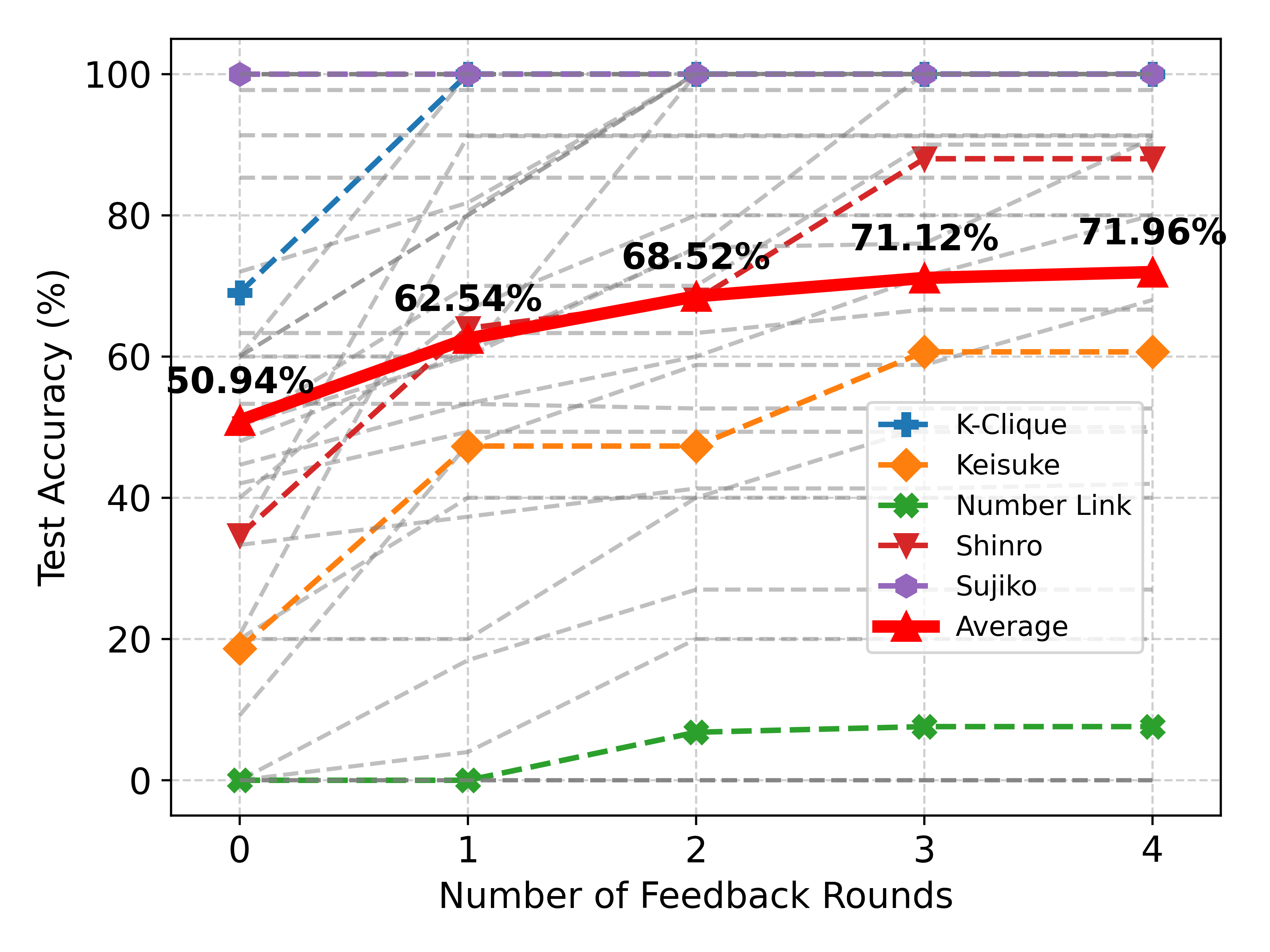
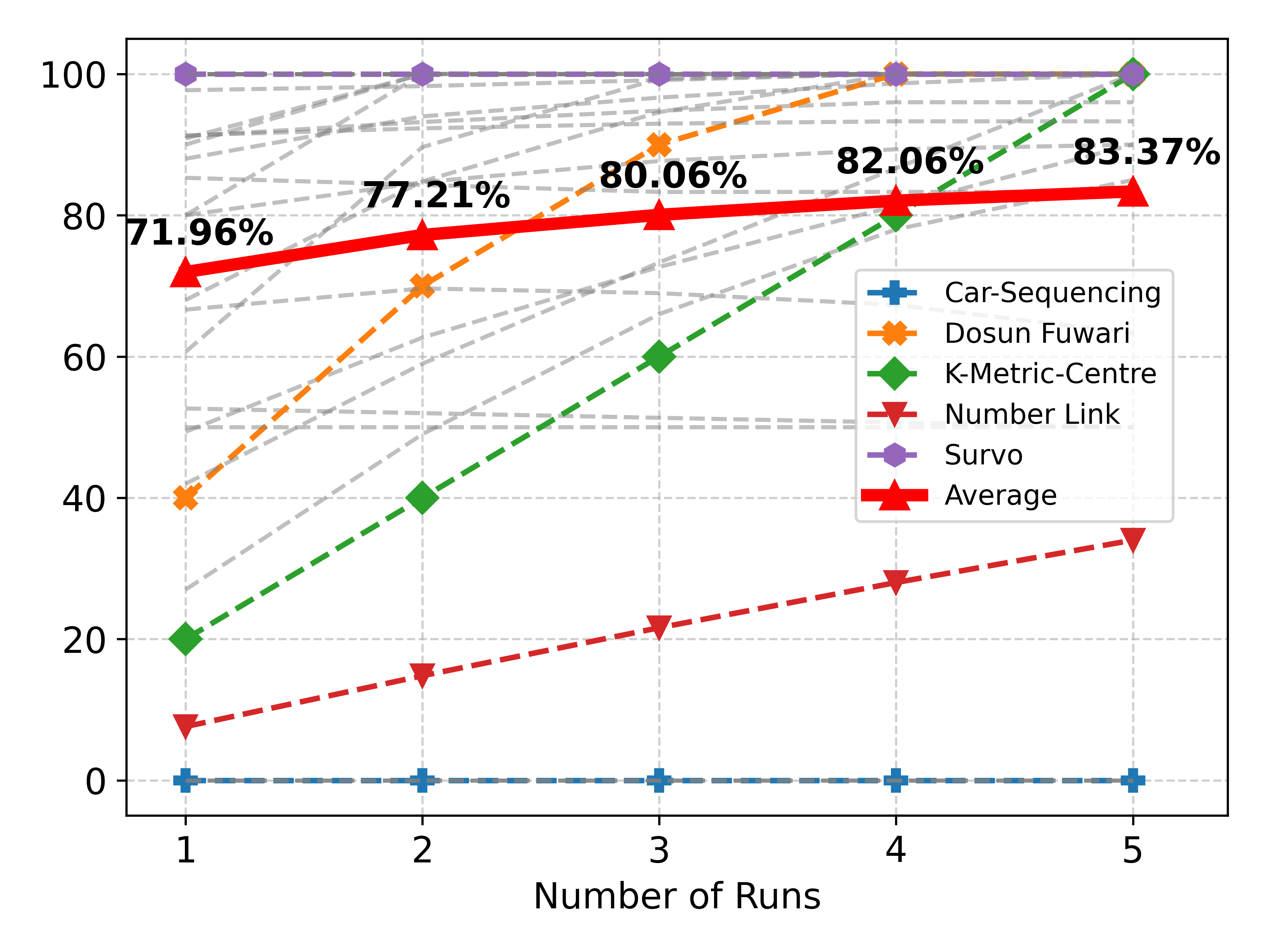
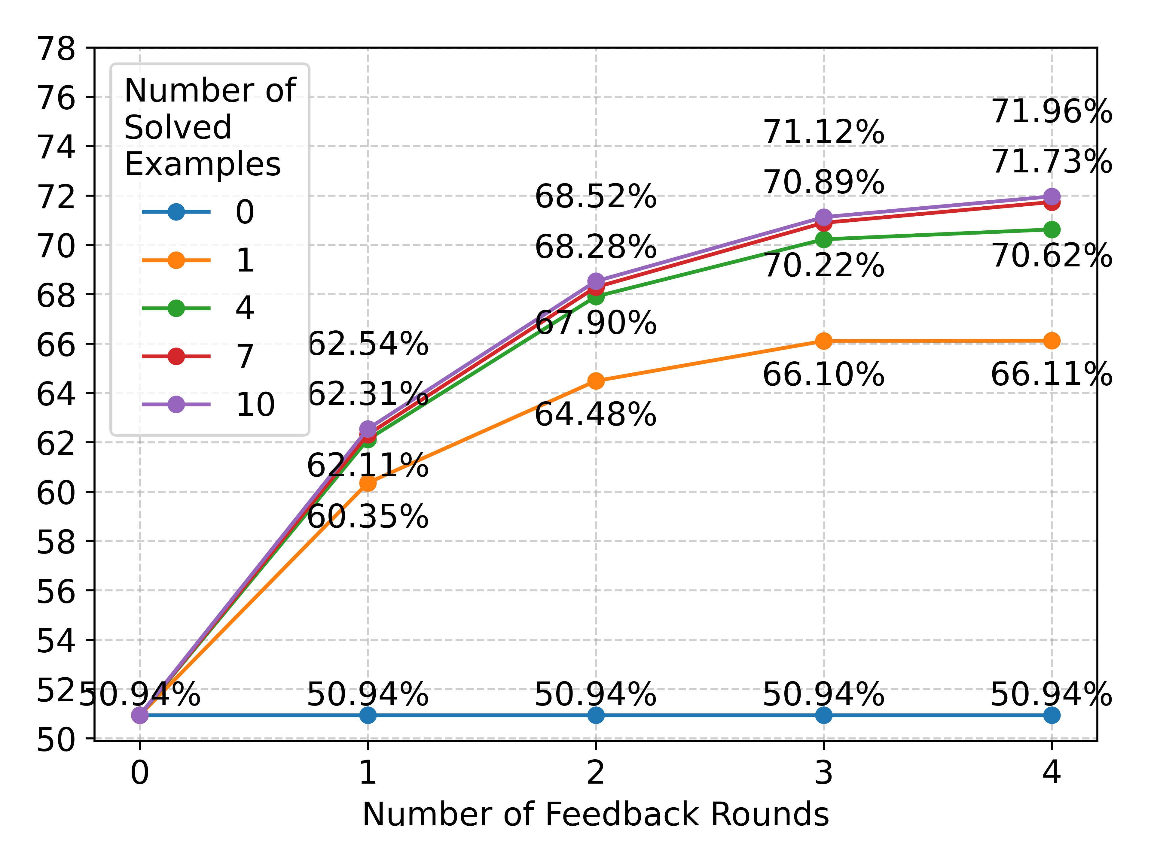
Figure 5: Effect of feedback and multiple runs with GPT-4-Turbo. (a) and (b) show results with 10 solved examples for feedback where dashed lines show results for individual problems in FCoReBench, with coloured lines highlighting specific problems and the red bold line represents the average effect across all problems. (c) shows the effect of number of solved examples used for feedback in a single run.
Effect of Feedback on Solved Examples: Figure 5(a) describes the effect of multiple rounds of feedback for SymPro-LM. Feedback helps performance significantly; utilizing 4 feedback rounds improves performance by $21.02\$ . Even the largest LLMs commit errors, making it important to verify and correct their work. But feedback on its own is not enough, a single run might end-up in a wrong reasoning path, which is not corrected by feedback making it important to utilize multiple runs for effective reasoning. Utilizing 5 runs improves the performance by additional $11.41\$ (Figure 5(b)) after which the gains tend to saturate. Performance also increases with an increase in the number of solved examples (Figure 5(c)). Each solved example helps in detecting and correcting different errors. However, performance tends to saturate at 7 solved examples and no new errors are discovered/corrected, even with additional training data.
### 7.1 Results on Other Datasets
Table 6: Results for baselines & SymPro-LM on other benchmarks. Best results with each LLM are highlighted.
| Logical Deduction ProofWriter PrOntoQA | 39.66 % 40.50 % 49.60 % | 50.66 % 57.16 % 83.20 % | 66.33 % 50.5 % 98.40 % | 71.00 % 70.16 % 72.20 % | 78.00 % 74.167 % 97.40 % | 65.33 % 46.5 % 83.00 % | 76.00 % 61.66 % 98.80 % | 81.66 % 76.29 % 99.80 % | 82.67 % 74.83 % 91.20 % | 94.00 % 89.83 % 97.80 % |
| --- | --- | --- | --- | --- | --- | --- | --- | --- | --- | --- |
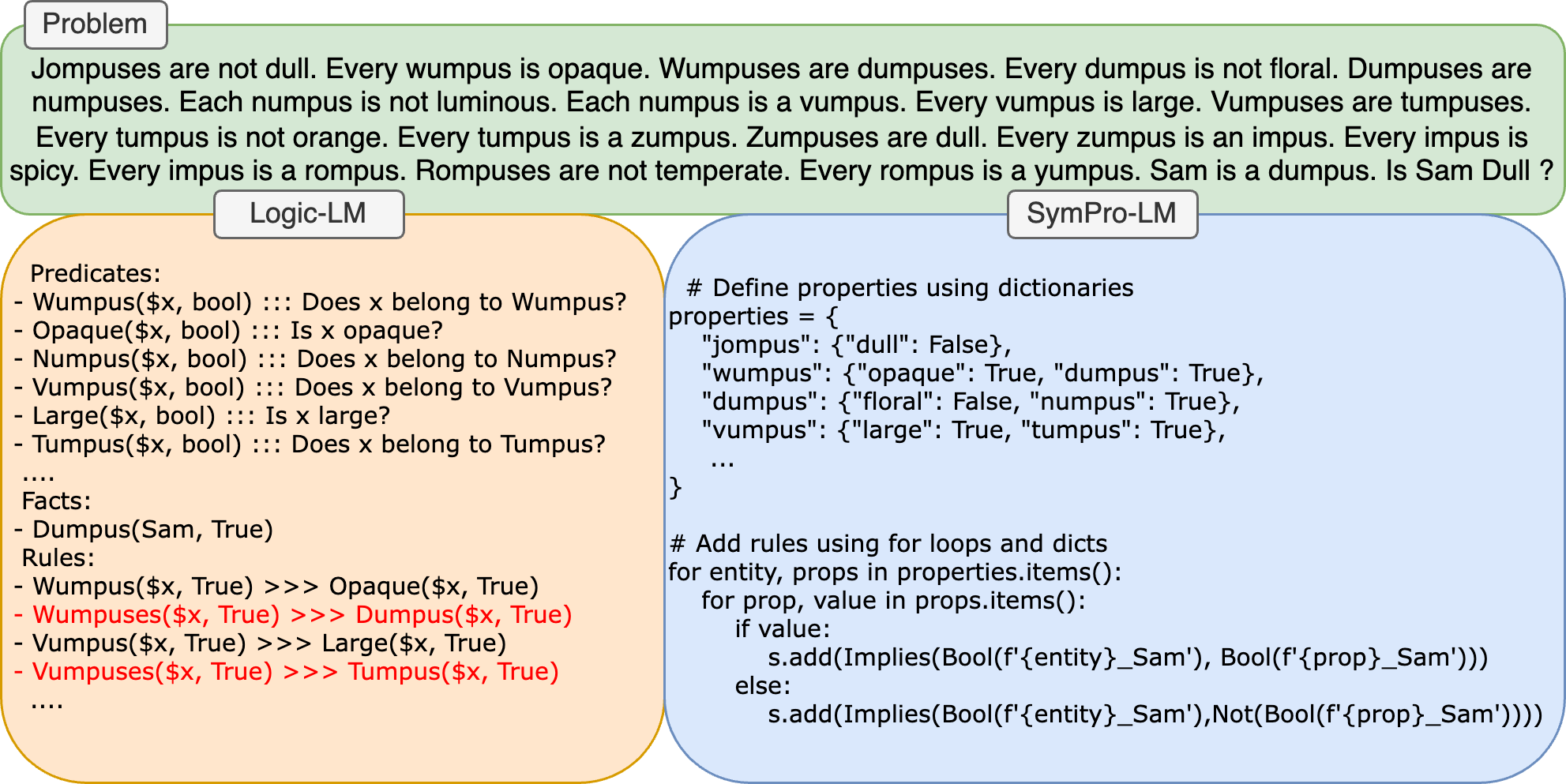
Table 6 reports the performance on non-first order datasets. SymPro-LM outperforms all other baselines on ProofWriter and LogicalDeduction, particularly Logic-LM. This showcases the value of integrating LLMs with symbolic solvers through programs, even for standard reasoning tasks. These experiments suggest that LLMs translate natural language questions into programs using solvers much more effectively than into symbolic formulations directly. We attribute this to the vast pre-training of LLMs on code (Brown et al., 2020; Chen et al., 2021). For instance, on the LogicalDeduction benchmark, while Logic-LM does not make syntactic errors during translation it often makes logical errors. These errors significantly decrease when LLMs are prompted to produce programs instead (Figure 6(b)). Error analysis on ProofWriter and PrOntoQA reveals that for more complex natural language questions, LLMs also start making syntactic errors during translation as the number of rules/facts start increasing. With SymPro-LM these errors are vastly reduced because, apart from the benefit from pre-training, LLMs also start utilizing programming constructs like dictionaries and loops to make most out of the structure in these problems (Figure 6(a)). PAL and CoT perform marginally better on PrOntoQA because the reasoning style for problems in this dataset involves forward-chain reasoning which aligns with PAL’s and CoT’s style of reasoning. Integrating symbolic solvers is not as useful for this dataset, but still achieves competitive performance.
<details>
<summary>extracted/6211530/Images/prontoQA-example.png Details</summary>
### Visual Description
## Logic Puzzle Diagram: Formalization Approaches
### Overview
The image presents a logic puzzle involving fictional creatures and their properties, followed by two different computational approaches to formalize and solve the puzzle: "Logic-LM" and "SymPro-LM". The diagram is structured into three distinct regions: a top "Problem" statement, a left "Logic-LM" panel, and a right "SymPro-LM" panel.
### Components/Axes
The diagram is not a chart with axes but a conceptual flow diagram with three main text blocks:
1. **Top Block (Green Background):** Labeled "Problem". Contains the full text of the logic puzzle.
2. **Left Block (Orange Background):** Labeled "Logic-LM". Contains a formal logical representation using predicates, facts, and rules.
3. **Right Block (Blue Background):** Labeled "SymPro-LM". Contains a symbolic programming representation using Python-like code with dictionaries and loops.
### Detailed Analysis / Content Details
#### 1. Problem Statement (Top Block)
**Text Transcription:**
"Jompuses are not dull. Every wumpus is opaque. Wumpuses are dumpuses. Every dumpus is not floral. Dumpuses are numpuses. Each numpus is not luminous. Each numpus is a vumpus. Every vumpus is large. Vumpuses are tumpuses. Every tumpus is not orange. Every tumpus is a zumpus. Zumpuses are dull. Every zumpus is an impus. Every impus is spicy. Every impus is a rompus. Rompuses are not temperate. Every rompus is a yumpus. Sam is a dumpus. Is Sam Dull?"
**Language:** English. The terms "jompuses", "wumpuses", etc., are fictional and not translated.
#### 2. Logic-LM Representation (Left Block)
This section formalizes the problem using first-order logic syntax.
**Predicates:**
- `Wumpus($x, bool) :: Does x belong to Wumpus?`
- `Opaque($x, bool) :: Is x opaque?`
- `Numpus($x, bool) :: Does x belong to Numpus?`
- `Vumpus($x, bool) :: Does x belong to Vumpus?`
- `Large($x, bool) :: Is x large?`
- `Tumpus($x, bool) :: Does x belong to Tumpus?`
- `....` (Indicates additional predicates are implied but not listed)
**Facts:**
- `Dumpus(Sam, True)`
**Rules (Implications):**
- `Wumpus($x, True) >>> Opaque($x, True)`
- `Wumpuses($x, True) >>> Dumpus($x, True)` (Text in red)
- `Vumpus($x, True) >>> Large($x, True)`
- `Vumpuses($x, True) >>> Tumpus($x, True)` (Text in red)
- `....` (Indicates additional rules are implied but not listed)
**Spatial Grounding:** The "Logic-LM" label is centered above its orange panel. The content is left-aligned within the panel. The rules are listed vertically, with two rules highlighted in red text.
#### 3. SymPro-LM Representation (Right Block)
This section formalizes the problem using a symbolic programming approach, resembling Python code.
**Code Transcription:**
```python
# Define properties using dictionaries
properties = {
"jompus": {"dull": False},
"wumpus": {"opaque": True, "dumpus": True},
"dumpus": {"floral": False, "numpus": True},
"vumpus": {"large": True, "tumpus": True},
...
}
# Add rules using for loops and dicts
for entity, props in properties.items():
for prop, value in props.items():
if value:
s.add(Implies(Bool(f'{entity}_Sam'), Bool(f'{prop}_Sam')))
else:
s.add(Implies(Bool(f'{entity}_Sam'),Not(Bool(f'{prop}_Sam'))))
```
**Spatial Grounding:** The "SymPro-LM" label is centered above its blue panel. The code is left-aligned within the panel. The `properties` dictionary is defined first, followed by the rule-generation loop.
### Key Observations
1. **Dual Formalization:** The core of the image is the side-by-side comparison of two distinct methods (logic-based vs. symbolic programming) for representing the same natural language problem.
2. **Incomplete Listings:** Both formalization panels use ellipses (`....` or `...`) to indicate that the provided lists of predicates, rules, and properties are not exhaustive but illustrative.
3. **Highlighted Rules:** In the Logic-LM panel, two specific rules (`Wumpuses($x, True) >>> Dumpus($x, True)` and `Vumpuses($x, True) >>> Tumpus($x, True)`) are displayed in red text, potentially indicating they are derived rules or of particular importance in the inference chain.
4. **Code Structure:** The SymPro-LM code uses a data-driven approach. The `properties` dictionary encodes the facts from the problem statement. The subsequent loop programmatically generates logical implication rules (`Implies`) for a solver (`s.add`), handling both positive (`True`) and negative (`False`) properties.
### Interpretation
This diagram serves as an educational or technical comparison between two AI/automated reasoning paradigms for solving logical puzzles.
* **What it demonstrates:** It shows how the same set of natural language statements ("Every A is B", "C is not D") can be translated into different formal representations suitable for computation. The Logic-LM approach mirrors traditional symbolic AI and formal logic. The SymPro-LM approach uses a more modern, programmatic style common in symbolic programming libraries.
* **Relationship between elements:** The "Problem" is the source material. Both "Logic-LM" and "SymPro-LM" are downstream, structured interpretations of that problem. They are parallel solutions to the same translation task. The red text in Logic-LM and the `...` in both panels suggest these are simplified excerpts from a fuller implementation.
* **Underlying puzzle:** The puzzle itself is a chain of set inclusions and property assignments. To answer "Is Sam Dull?", one must trace the implications: Sam is a dumpus -> dumpus is a numpus -> numpus is a vumpus -> vumpus is a tumpus -> tumpus is a zumpus -> zumpus is dull. Therefore, the logical conclusion is that Sam is dull. The formalizations are tools to reach this conclusion algorithmically.
* **Purpose of the diagram:** The primary goal is likely to illustrate the process of "formalizing" natural language for AI reasoning systems, highlighting different technical pathways (declarative logic vs. imperative code) to achieve the same goal. It emphasizes the importance of structured representation in problem-solving.
</details>
(a) PrOntoQA
<details>
<summary>extracted/6211530/Images/logicaldeduction-example.png Details</summary>
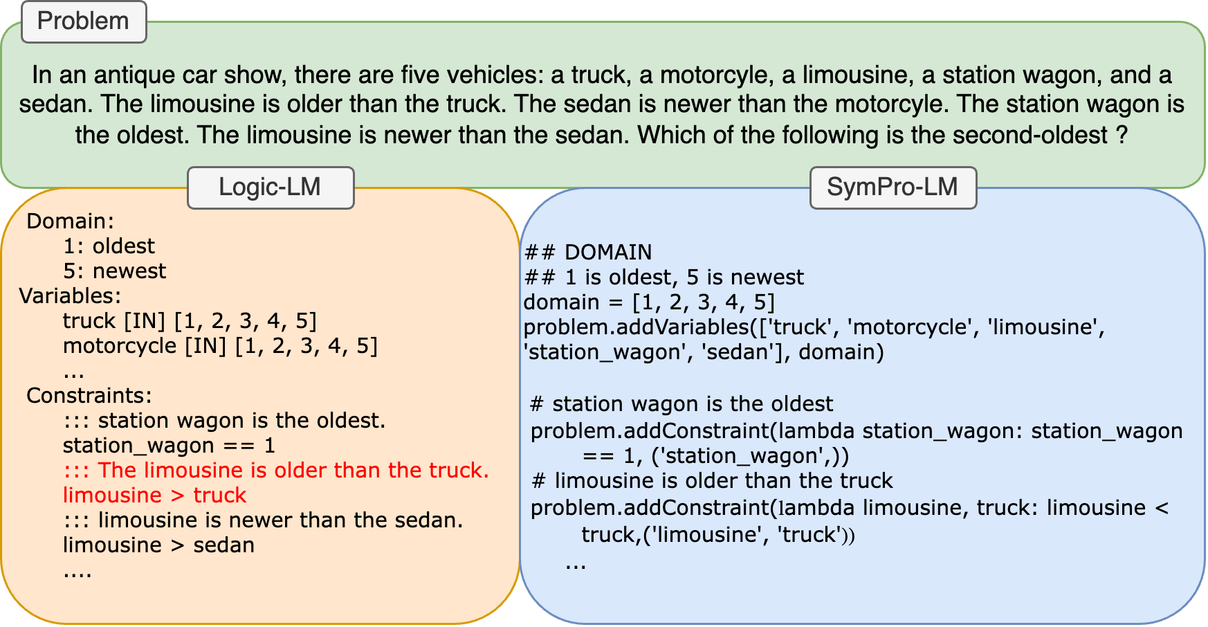
### Visual Description
## Logic Puzzle Diagram: Vehicle Age Ordering Problem
### Overview
The image presents a logic puzzle about ordering five antique vehicles by age, along with two different computational approaches to solving it: "Logic-LM" and "SymPro-LM". The diagram is structured with a problem statement at the top, followed by two solution panels side-by-side.
### Components/Axes
The image is divided into three main sections:
1. **Top Section (Green Box):** Contains the problem statement.
2. **Left Panel (Orange Box):** Labeled "Logic-LM", showing a formal logic representation.
3. **Right Panel (Blue Box):** Labeled "SymPro-LM", showing a Python-like constraint programming representation.
### Detailed Analysis
#### 1. Problem Statement (Top Green Box)
**Text Transcription:**
"Problem
In an antique car show, there are five vehicles: a truck, a motorcyle, a limousine, a station wagon, and a sedan. The limousine is older than the truck. The sedan is newer than the motorcyle. The station wagon is the oldest. The limousine is newer than the sedan. Which of the following is the second-oldest ?"
**Note:** The word "motorcycle" is consistently misspelled as "motorcyle" in the original text.
#### 2. Logic-LM Panel (Left Orange Box)
**Header:** "Logic-LM"
**Content Structure:**
* **Domain:**
* `1: oldest`
* `5: newest`
* **Variables:**
* `truck [IN] [1, 2, 3, 4, 5]`
* `motorcycle [IN] [1, 2, 3, 4, 5]`
* `...` (ellipsis indicates continuation)
* **Constraints:**
* `::: station wagon is the oldest.`
* `station_wagon == 1`
* `::: The limousine is older than the truck.` (This line is in **red text**)
* `limousine > truck`
* `::: limousine is newer than the sedan.`
* `limousine > sedan`
* `....` (ellipsis indicates continuation)
#### 3. SymPro-LM Panel (Right Blue Box)
**Header:** "SymPro-LM"
**Content Structure (Python-like code):**
```python
## DOMAIN
## 1 is oldest, 5 is newest
domain = [1, 2, 3, 4, 5]
problem.addVariables(['truck', 'motorcycle', 'limousine', 'station_wagon', 'sedan'], domain)
# station wagon is the oldest
problem.addConstraint(lambda station_wagon: station_wagon == 1, ('station_wagon',))
# limousine is older than the truck
problem.addConstraint(lambda limousine, truck: limousine < truck, ('limousine', 'truck'))
...
```
### Key Observations
1. **Inconsistent Constraint Representation:** There is a critical discrepancy in how the constraint "The limousine is older than the truck" is represented between the two panels.
* In **Logic-LM**, it is written as `limousine > truck`. Given the domain (1=oldest, 5=newest), this would mean the limousine's age number is *greater* than the truck's, implying the limousine is *newer*.
* In **SymPro-LM**, it is written as `limousine < truck`. This correctly translates to the limousine's age number being *smaller*, meaning it is *older*.
* The red text in the Logic-LM panel may be highlighting this specific constraint for attention.
2. **Partial Information:** Both solution panels use ellipses (`...` or `....`), indicating that not all variables or constraints from the full problem are displayed in this excerpt.
3. **Language:** The primary language is English. The SymPro-LM panel uses code syntax.
### Interpretation
This diagram illustrates two different formal methods for encoding and solving a logical reasoning problem. The puzzle itself is a classic constraint satisfaction problem.
* **What the Data Suggests:** The core task is to determine a unique ordering of five items based on relational clues. The provided snippets show the initial setup: defining a search space (domain 1-5), creating variables for each vehicle, and beginning to translate English sentences into formal logical or programmatic constraints.
* **Relationship Between Elements:** The "Problem" box is the source material. The "Logic-LM" and "SymPro-LM" boxes are parallel attempts to model that problem computationally. They share the same goal but use different syntactic frameworks.
* **Notable Anomaly:** The direct contradiction in the "limousine vs. truck" constraint between the two models is the most significant finding. This appears to be an error in the Logic-LM representation, as it contradicts the problem statement ("limousine is older"). The SymPro-LM version (`limousine < truck`) is logically consistent with the given domain definition.
* **Underlying Purpose:** The image likely serves an educational or demonstrative purpose, comparing how different AI or programming paradigms (symbolic logic vs. constraint programming) approach the same reasoning task. The inconsistency may be intentional to highlight common pitfalls in formalization.
**Puzzle Solution (for context):**
Based on the correct constraints:
1. Station Wagon = 1 (oldest)
2. Limousine > Sedan (Limousine is newer than Sedan)
3. Limousine < Truck (Limousine is older than Truck)
4. Sedan < Motorcycle (Sedan is newer than Motorcycle)
This leads to the order: **Station Wagon (1), Sedan (2), Limousine (3), Truck (4), Motorcycle (5)**. Therefore, the **second-oldest is the Sedan**.
</details>
(b) LogicalDeduction
Figure 6: Examples highlighting benefits of integrating LLMs with symbolic solver through programs.
## 8 Discussion
We analyze FCoReBench to identify where LLMs excel and where the largest models still struggle. Based on SymPro-LM ’s performance, we categorize FCoReBench problems into three broad groups.
1) Problems that SymPro-LM solved with 100% accuracy without any feedback. 8 such problems exist out of the $40$ , including vertex-cover and latin-square. These problems have a one-to-one correspondence between the natural language description of the rules and the program for generating the constraints and the LLM essentially has to perform a pure translation task which they excel at.
2) Problems that SymPro-LM solved with 100% accuracy but after feedback from solved examples. There are 20 such problems. They typically do not have a one-to-one correspondence between rule descriptions and code, thus requiring some reasoning to encode the problem in the solver’s language. For eg. one must define auxiliary variables and/or compose several primitives to encode a single natural language rule. GPT-4-Turbo initially misses constraints or encodes the problem incorrectly, but with feedback, it can spot its mistakes and corrects its programs. Examples include k-clique and binairo. In binairo, for example, GPT-4-Turbo incorrectly encodes the constraints for ensuring all columns and rows to be distinct but fixes this mistake after feedback (see Figure 17 in the appendix). LLMs can leverage their vast pre-training to discover non-trivial encodings for several interesting problems and solved examples can help guide LLMs to correct solutions in case of mistakes.
3) Problems with performance below 100% that are not corrected through feedback or utilizing multiple runs. For these 12 problems, LLM finds it difficult to encode some natural language constraint into SMT. Examples include number-link and hamiltonian path, where GPT-4-Turbo is not able to figure out how to encode existence of paths as SMT constraints. In our opinion, these conversions are peculiar, and may be hard even for average CS students. We hope that further analysis of these 12 domains opens up research directions for neuro-symbolic reasoning with LLMs.
## 9 Conclusion and Limitations
We investigate the reasoning abilities of LLMs on structured first-order combinatorial reasoning problems. We formally define the task, and we present FCoReBench, a novel benchmark of $40$ such problems and find that existing tool-augmented techniques, such as Logic-LM and PAL fare poorly. In response, we propose SymPro-LM – a new technique to aid LLMs with both program interpreters and symbolic solvers. It uses LLMs to convert text into executable code, which is then processed by interpreters to define constraints, allowing symbolic solvers to efficiently tackle the reasoning tasks. Our extensive experiments show that SymPro-LM ’s integrated approach leads to superior performance on our dataset as well as existing benchmarks. Error analysis reveals that SymPro-LM struggles for a certain class of problems where conversion to symbolic representation is not straightforward. In such cases simple feedback strategies do not improve reasoning; exploring methods to alleviate such problems is a promising direction for future work. Another future work direction is to extend this dataset to include images of inputs and outputs, instead of serialized text representations, and assess the reasoning abilities of vision-language models, like GPT4-V.
Limitations: While we study a wide variety of fcore problems, more such problems always exist and adding these to FCoReBench remains a direction of future work. Additionally we assume that input instances and their outputs have a fixed pre-defined (serialized) representation, which may not always be easy to find. Another limitation is that encoding of many problems in the solver’s language can potentially be complicated. Our method relies on the pre-training of LLMs to achieve this without any training/fine-tuning, and addressing this is a direction for future work.
## References
- bench authors [2023] BIG bench authors. Beyond the imitation game: Quantifying and extrapolating the capabilities of language models. Transactions on Machine Learning Research, 2023. ISSN 2835-8856.
- Brown et al. [2020] Tom Brown, Benjamin Mann, Nick Ryder, Melanie Subbiah, Jared D Kaplan, Prafulla Dhariwal, Arvind Neelakantan, Pranav Shyam, Girish Sastry, Amanda Askell, et al. Language models are few-shot learners. Advances in neural information processing systems, 33:1877–1901, 2020.
- Chen et al. [2021] Mark Chen, Jerry Tworek, Heewoo Jun, Qiming Yuan, Henrique Pondé de Oliveira Pinto, Jared Kaplan, Harrison Edwards, Yuri Burda, Nicholas Joseph, Greg Brockman, Alex Ray, Raul Puri, Gretchen Krueger, Michael Petrov, Heidy Khlaaf, Girish Sastry, Pamela Mishkin, Brooke Chan, Scott Gray, Nick Ryder, Mikhail Pavlov, Alethea Power, Lukasz Kaiser, Mohammad Bavarian, Clemens Winter, Philippe Tillet, Felipe Petroski Such, Dave Cummings, Matthias Plappert, Fotios Chantzis, Elizabeth Barnes, Ariel Herbert-Voss, William Hebgen Guss, Alex Nichol, Alex Paino, Nikolas Tezak, Jie Tang, Igor Babuschkin, Suchir Balaji, Shantanu Jain, William Saunders, Christopher Hesse, Andrew N. Carr, Jan Leike, Joshua Achiam, Vedant Misra, Evan Morikawa, Alec Radford, Matthew Knight, Miles Brundage, Mira Murati, Katie Mayer, Peter Welinder, Bob McGrew, Dario Amodei, Sam McCandlish, Ilya Sutskever, and Wojciech Zaremba. Evaluating large language models trained on code. CoRR, abs/2107.03374, 2021.
- Clark et al. [2021] Peter Clark, Oyvind Tafjord, and Kyle Richardson. Transformers as soft reasoners over language. In Proceedings of the Twenty-Ninth International Joint Conference on Artificial Intelligence, IJCAI’20, 2021. ISBN 9780999241165.
- Cobbe et al. [2021] Karl Cobbe, Vineet Kosaraju, Mohammad Bavarian, Mark Chen, Heewoo Jun, Lukasz Kaiser, Matthias Plappert, Jerry Tworek, Jacob Hilton, Reiichiro Nakano, Christopher Hesse, and John Schulman. Training verifiers to solve math word problems. CoRR, abs/2110.14168, 2021.
- Colbourn [1984] Charles J. Colbourn. The complexity of completing partial latin squares. Discrete Applied Mathematics, 8(1):25–30, 1984. ISSN 0166-218X. doi: https://doi.org/10.1016/0166-218X(84)90075-1.
- De Biasi [2013] Marzio De Biasi. Binary puzzle is np–complete, 07 2013.
- De Moura and Bjørner [2008] Leonardo De Moura and Nikolaj Bjørner. Z3: An efficient smt solver. In International conference on Tools and Algorithms for the Construction and Analysis of Systems, pages 337–340. Springer, 2008.
- Demaine and Rudoy [2018] Erik D. Demaine and Mikhail Rudoy. Theoretical Computer Science, 732:80–84, 2018. ISSN 0304-3975. doi: https://doi.org/10.1016/j.tcs.2018.04.031.
- Epstein [1987] D. Epstein. On the np-completeness of cryptarithms. ACM SIGACT News, 18(3):38–40, 1987. doi: 10.1145/24658.24662.
- Fan et al. [2023] Lizhou Fan, Wenyue Hua, Lingyao Li, Haoyang Ling, and Yongfeng Zhang. Nphardeval: Dynamic benchmark on reasoning ability of large language models via complexity classes. arXiv preprint arXiv:2312.14890, 2023.
- Gao et al. [2023] Luyu Gao, Aman Madaan, Shuyan Zhou, Uri Alon, Pengfei Liu, Yiming Yang, Jamie Callan, and Graham Neubig. Pal: Program-aided language models. In International Conference on Machine Learning, pages 10764–10799. PMLR, 2023.
- Garey et al. [1976a] M. R. Garey, D. S. Johnson, and Ravi Sethi. The complexity of flowshop and jobshop scheduling. Mathematics of Operations Research, 1(2):117–129, 1976a. doi: 10.1287/moor.1.2.117.
- Garey et al. [1976b] M. R. Garey, D. S. Johnson, and Ravi Sethi. The complexity of flowshop and jobshop scheduling. Mathematics of Operations Research, 1(2):117–129, 1976b. ISSN 0364765X, 15265471.
- Gent et al. [2017] Ian P. Gent, Christopher Jefferson, and Peter Nightingale. Complexity of n-queens completion. Journal of Artificial Intelligence Research (JAIR), 58:1–16, 2017. doi: 10.1613/jair.5512.
- Han et al. [2022] Simeng Han, Hailey Schoelkopf, Yilun Zhao, Zhenting Qi, Martin Riddell, Luke Benson, Lucy Sun, Ekaterina Zubova, Yujie Qiao, Matthew Burtell, David Peng, Jonathan Fan, Yixin Liu, Brian Wong, Malcolm Sailor, Ansong Ni, Linyong Nan, Jungo Kasai, Tao Yu, Rui Zhang, Shafiq R. Joty, Alexander R. Fabbri, Wojciech Kryscinski, Xi Victoria Lin, Caiming Xiong, and Dragomir Radev. FOLIO: natural language reasoning with first-order logic. CoRR, abs/2209.00840, 2022. doi: 10.48550/ARXIV.2209.00840.
- Hao et al. [2023] Shibo Hao, Yi Gu, Haodi Ma, Joshua Jiahua Hong, Zhen Wang, Daisy Zhe Wang, and Zhiting Hu. Reasoning with language model is planning with world model, 2023.
- Haraguchi and Ono [2015] Kazuya Haraguchi and Hirotaka Ono. How simple algorithms can solve latin square completion-type puzzles approximately. Journal of Information Processing, 23(3):276–283, 2015. doi: 10.2197/ipsjjip.23.276.
- HIGUCHI and KIMURA [2019] Yuta HIGUCHI and Kei KIMURA. Np-completeness of fill-a-pix and completeness of its fewest clues problem. IEICE Transactions on Fundamentals of Electronics, Communications and Computer Sciences, E102.A(11):1490–1496, 2019. doi: 10.1587/transfun.E102.A.1490.
- Itai et al. [1982] Alon Itai, Christos H. Papadimitriou, and Jayme Luiz Szwarcfiter. Hamilton paths in grid graphs. SIAM Journal on Computing, 11(4):676–686, 1982. doi: 10.1137/0211056.
- Iwamoto and Ibusuki [2018] Chuzo Iwamoto and Tatsuaki Ibusuki. Dosun-fuwari is np-complete. Journal of Information Processing, 26:358–361, 2018. doi: 10.2197/ipsjjip.26.358.
- Jiang et al. [2024] Albert Q. Jiang, Alexandre Sablayrolles, Antoine Roux, Arthur Mensch, Blanche Savary, Chris Bamford, Devendra Singh Chaplot, Diego de las Casas, Emma Bou Hanna, Florian Bressand, Gianna Lengyel, Guillaume Bour, Guillaume Lample, Lélio Renard Lavaud, Lucile Saulnier, Marie-Anne Lachaux, Pierre Stock, Sandeep Subramanian, Sophia Yang, Szymon Antoniak, Teven Le Scao, Théophile Gervet, Thibaut Lavril, Thomas Wang, Timothée Lacroix, and William El Sayed. Mixtral of experts, 2024.
- Kis [2004] Tamás Kis. On the complexity of the car sequencing problem. Operations Research Letters, 32(4):331–335, 2004. ISSN 0167-6377. doi: https://doi.org/10.1016/j.orl.2003.09.003.
- Kojima et al. [2022] Takeshi Kojima, Shixiang Shane Gu, Machel Reid, Yutaka Matsuo, and Yusuke Iwasawa. Large language models are zero-shot reasoners. In Sanmi Koyejo, S. Mohamed, A. Agarwal, Danielle Belgrave, K. Cho, and A. Oh, editors, Advances in Neural Information Processing Systems 35: Annual Conference on Neural Information Processing Systems 2022, NeurIPS 2022, New Orleans, LA, USA, November 28 - December 9, 2022, 2022.
- Liu et al. [2020] Jian Liu, Leyang Cui, Hanmeng Liu, Dandan Huang, Yile Wang, and Yue Zhang. Logiqa: A challenge dataset for machine reading comprehension with logical reasoning. In Christian Bessiere, editor, Proceedings of the Twenty-Ninth International Joint Conference on Artificial Intelligence, IJCAI 2020, pages 3622–3628. ijcai.org, 2020. doi: 10.24963/IJCAI.2020/501.
- Lloyd et al. [2022] Huw Lloyd, Matthew Crossley, Mark Sinclair, and Martyn Amos. J-pop: Japanese puzzles as optimization problems. IEEE Transactions on Games, 14(3):391–402, 2022. doi: 10.1109/TG.2021.3081817.
- Nandwani et al. [2021] Yatin Nandwani, Deepanshu Jindal, Mausam, and Parag Singla. Neural learning of one-of-many solutions for combinatorial problems in structured output spaces. In 9th International Conference on Learning Representations, ICLR 2021, Virtual Event, Austria, May 3-7, 2021. OpenReview.net, 2021.
- Nandwani et al. [2022a] Yatin Nandwani, Vidit Jain, Mausam, and Parag Singla. Neural models for output-space invariance in combinatorial problems. In The Tenth International Conference on Learning Representations, ICLR 2022, Virtual Event, April 25-29, 2022. OpenReview.net, 2022a.
- Nandwani et al. [2022b] Yatin Nandwani, Rishabh Ranjan, Mausam, and Parag Singla. A solver-free framework for scalable learning in neural ILP architectures. In Sanmi Koyejo, S. Mohamed, A. Agarwal, Danielle Belgrave, K. Cho, and A. Oh, editors, Advances in Neural Information Processing Systems 35: Annual Conference on Neural Information Processing Systems 2022, NeurIPS 2022, New Orleans, LA, USA, November 28 - December 9, 2022, 2022b.
- OpenAI [2023] OpenAI. Gpt-4 technical report, 2023.
- Palm et al. [2018] Rasmus Berg Palm, Ulrich Paquet, and Ole Winther. Recurrent relational networks. In Samy Bengio, Hanna M. Wallach, Hugo Larochelle, Kristen Grauman, Nicolò Cesa-Bianchi, and Roman Garnett, editors, Advances in Neural Information Processing Systems 31: Annual Conference on Neural Information Processing Systems 2018, NeurIPS 2018, December 3-8, 2018, Montréal, Canada, pages 3372–3382, 2018.
- Pan et al. [2023] Liangming Pan, Alon Albalak, Xinyi Wang, and William Wang. Logic-lm: Empowering large language models with symbolic solvers for faithful logical reasoning. In Houda Bouamor, Juan Pino, and Kalika Bali, editors, Findings of the Association for Computational Linguistics: EMNLP 2023, Singapore, December 6-10, 2023, pages 3806–3824. Association for Computational Linguistics, 2023.
- Paranjape et al. [2023] Bhargavi Paranjape, Scott M. Lundberg, Sameer Singh, Hannaneh Hajishirzi, Luke Zettlemoyer, and Marco Túlio Ribeiro. ART: automatic multi-step reasoning and tool-use for large language models. CoRR, abs/2303.09014, 2023. doi: 10.48550/ARXIV.2303.09014.
- Paulus et al. [2021] Anselm Paulus, Michal Rolínek, Vít Musil, Brandon Amos, and Georg Martius. Comboptnet: Fit the right np-hard problem by learning integer programming constraints. In Marina Meila and Tong Zhang, editors, Proceedings of the 38th International Conference on Machine Learning, ICML 2021, 18-24 July 2021, Virtual Event, volume 139 of Proceedings of Machine Learning Research, pages 8443–8453. PMLR, 2021.
- Russell and Norvig [2010] Stuart Russell and Peter Norvig. Artificial Intelligence: A Modern Approach. Prentice Hall, 3 edition, 2010.
- Saparov and He [2023a] Abulhair Saparov and He He. Language models are greedy reasoners: A systematic formal analysis of chain-of-thought. In The Eleventh International Conference on Learning Representations, ICLR 2023, Kigali, Rwanda, May 1-5, 2023. OpenReview.net, 2023a.
- Saparov and He [2023b] Abulhair Saparov and He He. Language models are greedy reasoners: A systematic formal analysis of chain-of-thought. In The Eleventh International Conference on Learning Representations, ICLR 2023, Kigali, Rwanda, May 1-5, 2023. OpenReview.net, 2023b.
- Schick et al. [2023] Timo Schick, Jane Dwivedi-Yu, Roberto Dessì, Roberta Raileanu, Maria Lomeli, Luke Zettlemoyer, Nicola Cancedda, and Thomas Scialom. Toolformer: Language models can teach themselves to use tools. CoRR, abs/2302.04761, 2023. doi: 10.48550/ARXIV.2302.04761.
- Tafjord et al. [2021] Oyvind Tafjord, Bhavana Dalvi, and Peter Clark. Proofwriter: Generating implications, proofs, and abductive statements over natural language. In Chengqing Zong, Fei Xia, Wenjie Li, and Roberto Navigli, editors, Findings of the Association for Computational Linguistics: ACL/IJCNLP 2021, Online Event, August 1-6, 2021, volume ACL/IJCNLP 2021 of Findings of ACL, pages 3621–3634. Association for Computational Linguistics, 2021. doi: 10.18653/V1/2021.FINDINGS-ACL.317.
- Wang et al. [2023] Heng Wang, Shangbin Feng, Tianxing He, Zhaoxuan Tan, Xiaochuang Han, and Yulia Tsvetkov. Can language models solve graph problems in natural language? In Thirty-seventh Conference on Neural Information Processing Systems, 2023.
- Wang et al. [2019] Po-Wei Wang, Priya Donti, Bryan Wilder, and Zico Kolter. SATNet: Bridging deep learning and logical reasoning using a differentiable satisfiability solver. In Kamalika Chaudhuri and Ruslan Salakhutdinov, editors, Proceedings of the 36th International Conference on Machine Learning, volume 97 of Proceedings of Machine Learning Research, pages 6545–6554. PMLR, 09–15 Jun 2019.
- Wei et al. [2022a] Jason Wei, Yi Tay, Rishi Bommasani, Colin Raffel, Barret Zoph, Sebastian Borgeaud, Dani Yogatama, Maarten Bosma, Denny Zhou, Donald Metzler, Ed H. Chi, Tatsunori Hashimoto, Oriol Vinyals, Percy Liang, Jeff Dean, and William Fedus. Emergent abilities of large language models. Trans. Mach. Learn. Res., 2022, 2022a.
- Wei et al. [2022b] Jason Wei, Yi Tay, Rishi Bommasani, Colin Raffel, Barret Zoph, Sebastian Borgeaud, Dani Yogatama, Maarten Bosma, Denny Zhou, Donald Metzler, Ed H. Chi, Tatsunori Hashimoto, Oriol Vinyals, Percy Liang, Jeff Dean, and William Fedus. Emergent abilities of large language models. Trans. Mach. Learn. Res., 2022, 2022b.
- Wei et al. [2022c] Jason Wei, Xuezhi Wang, Dale Schuurmans, Maarten Bosma, Fei Xia, Ed Chi, Quoc V Le, Denny Zhou, et al. Chain-of-thought prompting elicits reasoning in large language models. Advances in Neural Information Processing Systems, 35:24824–24837, 2022c.
- Yang et al. [2022] Kaiyu Yang, Jia Deng, and Danqi Chen. Generating natural language proofs with verifier-guided search. In Yoav Goldberg, Zornitsa Kozareva, and Yue Zhang, editors, Proceedings of the 2022 Conference on Empirical Methods in Natural Language Processing, pages 89–105, Abu Dhabi, United Arab Emirates, December 2022. Association for Computational Linguistics. doi: 10.18653/v1/2022.emnlp-main.7.
- Yao et al. [2023] Shunyu Yao, Dian Yu, Jeffrey Zhao, Izhak Shafran, Thomas L. Griffiths, Yuan Cao, and Karthik Narasimhan. Tree of thoughts: Deliberate problem solving with large language models. CoRR, abs/2305.10601, 2023. doi: 10.48550/ARXIV.2305.10601.
- YATO and SETA [2003] Takayuki YATO and Takahiro SETA. Complexity and completeness of finding another solution and its application to puzzles. IEICE Transactions on Fundamentals of Electronics, Communications and Computer Sciences, E86-A, 05 2003.
- Ye et al. [2023] Xi Ye, Qiaochu Chen, Isil Dillig, and Greg Durrett. Satlm: Satisfiability-aided language models using declarative prompting. In Proceedings of NeurIPS, 2023.
- Yu et al. [2023] Dongran Yu, Bo Yang, Dayou Liu, Hui Wang, and Shirui Pan. A survey on neural-symbolic learning systems. Neural Networks, 166:105–126, 2023. doi: 10.1016/J.NEUNET.2023.06.028.
- Zheng et al. [2023] Chuanyang Zheng, Zhengying Liu, Enze Xie, Zhenguo Li, and Yu Li. Progressive-hint prompting improves reasoning in large language models. CoRR, abs/2304.09797, 2023. doi: 10.48550/ARXIV.2304.09797.
- Zhong et al. [2021] Wanjun Zhong, Siyuan Wang, Duyu Tang, Zenan Xu, Daya Guo, Jiahai Wang, Jian Yin, Ming Zhou, and Nan Duan. AR-LSAT: investigating analytical reasoning of text. CoRR, abs/2104.06598, 2021.
- Zhou et al. [2023] Denny Zhou, Nathanael Schärli, Le Hou, Jason Wei, Nathan Scales, Xuezhi Wang, Dale Schuurmans, Claire Cui, Olivier Bousquet, Quoc V. Le, and Ed H. Chi. Least-to-most prompting enables complex reasoning in large language models. In The Eleventh International Conference on Learning Representations, ICLR 2023, Kigali, Rwanda, May 1-5, 2023. OpenReview.net, 2023.
## Appendix A FCoReBench
### A.1 Dataset Details and Statistics
Our dataset namely FCoReBench has $40$ different fcore problems that have been collected from various sources. Some of these problems are logical-puzzles from publishing houses like Nikoli, some problems are from operations research literature, some are from the annual SAT competition and other problems are well-known computational problems from Computer Science literature such as hamiltonian path and minimum-dominating set. Table 7 gives the details of all problems in our dataset. To create our training and test sets, we write scripts to synthetically generate problem instances. These can be used to extend the dataset as needed with any number of instances of any size. For experimentation, we generate some solved training instances and a separate set of testing instances. Each problem also has a natural language description of its rules, and a natural language description of the input-format which specify how input problem instances and their solutions are represented in text. The next few sections give illustrative examples and other details.
### A.2 Natural Language Description of Rules
This section describes how we create the natural language description of rules for problems in FCoReBench. We extract rules from the sources such as the Wikipedia/Nikoli pages of the corresponding problems. These rules are reworded by a human expert to reduce dataset contamination. Another human expert ensures that there are no ambiguities in the reworded description of the rules. The rules are generalized, when needed (for eg. from a $9× 9$ Sudoku to a $n× n$ Sudoku). The following sections provide few examples.
#### A.2.1 Example Problem: Survo
<details>
<summary>extracted/6211530/Images/survo-example.png Details</summary>
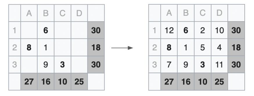
### Visual Description
## Diagram: Grid Transformation Puzzle
### Overview
The image displays a side-by-side comparison of two 3x4 grids (tables) with an arrow pointing from the left grid to the right grid, indicating a transformation or solution process. The grids have rows labeled 1, 2, 3 and columns labeled A, B, C, D. The final column (after D) and the bottom row are shaded gray and contain numbers, which appear to be row and column totals, respectively. The left grid shows a partially filled set of cells, while the right grid shows the same grid with all cells filled in, satisfying the given totals.
### Components/Axes
- **Grid Structure**: Both grids are identical in layout.
- **Rows**: Labeled 1, 2, 3 on the left side.
- **Columns**: Labeled A, B, C, D at the top.
- **Shaded Cells**: The rightmost column (unlabeled, but after column D) and the bottom row (unlabeled, but below row 3) are shaded gray and contain numbers.
- **Arrow**: A black arrow points from the center of the left grid to the center of the right grid, indicating a directional relationship (e.g., problem to solution).
- **Labels**: All row and column labels (1,2,3 and A,B,C,D) are in a light gray font.
### Detailed Analysis
#### Left Grid (Initial State)
This grid contains some pre-filled numbers and blank cells. The shaded totals are provided.
| | A | B | C | D | **Total (Shaded)** |
|-----|-----|-----|-----|-----|-------------------|
| **1** | | **6** | | | **30** |
| **2** | **8** | **1** | | | **18** |
| **3** | | **9** | **3** | | **30** |
| **Total (Shaded)** | **27** | **16** | **10** | **25** | |
*Missing Cells*: A1, C1, D1, C2, D2, A3, D3. (7 cells total)
#### Right Grid (Final State)
This grid is completely filled. All shaded totals remain identical to the left grid, confirming they are constraints.
| | A | B | C | D | **Total (Shaded)** |
|-----|-----|-----|-----|-----|-------------------|
| **1** | **12** | **6** | **2** | **10** | **30** |
| **2** | **8** | **1** | **5** | **4** | **18** |
| **3** | **7** | **9** | **3** | **11** | **30** |
| **Total (Shaded)** | **27** | **16** | **10** | **25** | |
*Verification of Totals*:
- **Row Sums**:
- Row 1: 12 + 6 + 2 + 10 = 30 ✓
- Row 2: 8 + 1 + 5 + 4 = 18 ✓
- Row 3: 7 + 9 + 3 + 11 = 30 ✓
- **Column Sums**:
- Column A: 12 + 8 + 7 = 27 ✓
- Column B: 6 + 1 + 9 = 16 ✓
- Column C: 2 + 5 + 3 = 10 ✓
- Column D: 10 + 4 + 11 = 25 ✓
### Key Observations
1. **Constraint Consistency**: The shaded totals (row and column sums) are identical in both grids, acting as fixed constraints for the puzzle.
2. **Unique Solution**: The left grid's partial data, combined with the totals, leads to a single, consistent solution shown in the right grid. All missing values are positive integers.
3. **Spatial Layout**: The legend (shaded totals) is positioned at the right and bottom edges of each grid. The arrow is centrally placed between the two grids.
4. **Data Integrity**: Every number in the right grid precisely satisfies the row and column sum constraints from the left grid. No outliers or inconsistencies are present.
### Interpretation
This diagram illustrates a classic **grid-filling puzzle** or a **system of linear equations** with integer solutions. The left grid presents a problem: given some initial numbers and the required sums for each row and column, find the missing values. The right grid provides the solution.
The puzzle demonstrates how constraints (the totals) propagate through the grid to determine unknown values uniquely. For example:
- The value in cell A1 (12) is derived from the column A total (27) minus the known values in A2 (8) and A3 (7).
- Similarly, cell D1 (10) comes from the row 1 total (30) minus the known B1 (6) and the derived A1 (12) and C1 (2).
This type of puzzle is often used in logic games, educational settings to teach arithmetic and algebra, or as a constraint satisfaction problem in computer science. The transformation from left to right visually confirms that the solution is correct and complete, with all constraints satisfied. The absence of negative numbers or fractions suggests the puzzle is designed for simplicity and clarity.
</details>
Figure 7: Conversion of an input survo problem instance to its solution.
Survo (Figure 7) is an example problem from FCoReBench. The task is to fill a $m× n$ rectangular board with numbers from $1-m*n$ such that each row and column sums to an intended target. (Survo-Wikipedia). The box given below describes the rules of Survo more formally in natural language.
We are given a partially filled $m× n$ rectangular board, intended row sums and column sums. - Empty cells are to be filled with numbers - Numbers in the solved board can range from $1$ to $m*n$ - Numbers present in filled cells on the input board cannot be removed - Each number from 1 to m*n must appear exactly once on the solved board - All the empty cells should be filled such that each row and each column of the solved board must sum to the respective row sum and column sum as specified in the input
#### A.2.2 Example Problem: Hamiltonian Path
<details>
<summary>extracted/6211530/Images/hamiltonian-path-example.png Details</summary>
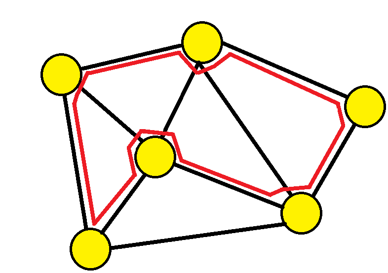
### Visual Description
\n
## Diagram: Network Graph with Highlighted Path
### Overview
The image displays a simple undirected graph diagram consisting of six nodes (vertices) connected by edges (lines). A specific path through the graph is highlighted in red. There is no textual information, labels, titles, or legends present in the image.
### Components/Axes
* **Nodes:** Six identical, solid yellow circles with black outlines. They are arranged in a roughly hexagonal pattern with one node positioned centrally.
* **Edges:** Straight black lines connecting the nodes, representing the graph's structure. The graph is fully connected in a mesh-like topology.
* **Highlighted Path:** A thick, continuous red line that traces a specific route through the graph, overlaying some of the black edges.
### Detailed Analysis
**Graph Structure:**
The six nodes are positioned as follows (using approximate clock-face positions for reference):
1. Top-Left
2. Top-Center
3. Top-Right
4. Center
5. Bottom-Left
6. Bottom-Right
The black edges connect the nodes to form a network. The central node is connected to all five outer nodes. The outer nodes are also connected to their immediate neighbors, forming a perimeter.
**Highlighted Red Path:**
The red line traces a continuous path through the graph. Its route is as follows:
1. Starts at the **Top-Left** node.
2. Travels along the edge to the **Center** node.
3. From the Center node, it travels to the **Bottom-Right** node.
4. From the Bottom-Right node, it travels to the **Top-Right** node.
5. From the Top-Right node, it travels to the **Top-Center** node.
6. From the Top-Center node, it travels back to the **Center** node.
7. Finally, from the Center node, it travels to the **Bottom-Left** node, where the path ends.
This creates a path that visits five of the six nodes (all except the Top-Left node is visited only at the start, and the path does not return to it). The path revisits the central node twice.
### Key Observations
* The diagram is purely structural and contains no quantitative data, labels, or annotations.
* The red path is the only element that provides a specific narrative or sequence to the graph.
* The graph is planar (can be drawn without edges crossing), and the red path does not cross any edges it is not traveling along.
* The central node acts as a hub, being part of the red path three times (start, middle, and end segments).
### Interpretation
This diagram is an abstract representation of a network or a set of relationships. The yellow nodes could represent entities (e.g., computers, cities, people, states), and the black edges represent connections or relationships between them.
The red line highlights a specific **traversal, circuit, or route** through this network. Given that it starts and ends at different nodes and revisits the central hub, it could illustrate:
* A data packet's journey in a computer network.
* A logistics or travel route.
* A sequence of steps in a process or algorithm (like a depth-first search path).
* A critical path or a highlighted connection sequence in a system.
The absence of labels means the specific context is unknown. However, the visual structure clearly communicates the concept of a connected system and a defined path within it. The central node's importance is emphasized by its multiple connections and its role as a junction in the highlighted route.
</details>
Figure 8: A sample input graph instance and its solution to the hamiltonian-path problem. Vertices are represented by yellow circles and the hamiltonian path is represented by the red line.
Hamiltonian path is a well-known problem in graph theory in which we have to find a path in an un-directed and an un-weighted graph such that each vertex is visited exactly once by the path. We consider the decision variant of this problem which is equally hard in terms of computational complexity. The box below shows the formal rules for this problem expressed in natural language.
We are given an un-directed and un-weighted graph. - We have to determine if the graph contains a path that visits every vertex exactly once.
#### A.2.3 Example Problem: Dosun Fuwari
<details>
<summary>extracted/6211530/Images/dosun-fuwari-example.png Details</summary>

### Visual Description
## Diagram: Before-and-After Grid Transformation
### Overview
The image displays a two-panel diagram illustrating a transformation process. On the left is an initial 4x4 grid state, and on the right is the resulting state after an unspecified operation, indicated by a right-pointing arrow between them. The grids are composed of cells, some of which are filled with solid black squares. The transformed grid introduces circular markers (white/hollow and black/filled) into previously empty cells.
### Components/Axes
* **Structure:** Two 4x4 grids. Each grid is subdivided by thicker lines into four 2x2 quadrants.
* **Left Grid (Initial State):**
* Contains two solid black squares.
* All other cells are empty (white).
* **Right Grid (Transformed State):**
* Retains the two original solid black squares in their exact positions.
* Introduces circular markers into previously empty cells:
* **White (Hollow) Circles:** 5 instances.
* **Black (Filled) Circles:** 5 instances.
* **Arrow:** A simple, black, right-pointing arrow (`→`) centered between the two grids, indicating the direction of transformation.
* **Text:** No textual labels, titles, or annotations are present in the image.
### Detailed Analysis
**Spatial Mapping and Element Placement:**
(Using (Row, Column) notation, where Row 1 is the top row and Column 1 is the leftmost column.)
**1. Left Grid (Initial State):**
* **Black Squares:** Located at positions (2, 2) and (4, 4).
* **Empty Cells:** All other 14 positions.
**2. Right Grid (Transformed State):**
* **Persistent Black Squares:** Remain at (2, 2) and (4, 4).
* **White (Hollow) Circles:** Placed at:
* (1, 1) - Top-left quadrant
* (1, 4) - Top-right quadrant
* (2, 1) - Top-left quadrant
* (2, 4) - Top-right quadrant
* (3, 2) - Bottom-left quadrant
* **Black (Filled) Circles:** Placed at:
* (1, 2) - Top-left quadrant
* (3, 3) - Bottom-right quadrant
* (3, 4) - Bottom-right quadrant
* (4, 1) - Bottom-left quadrant
* (4, 3) - Bottom-right quadrant
**Transformation Summary:** The operation populates 10 of the 14 originally empty cells with circles. The distribution is not uniform: the top two quadrants receive only white circles (except for one black circle at (1,2)), while the bottom two quadrants receive a mix, with a concentration of black circles in the bottom-right quadrant.
### Key Observations
1. **Conservation:** The two original black squares are immutable anchors in the transformation.
2. **Pattern Introduction:** The transformation introduces a new layer of information (circles) without altering the base grid structure.
3. **Asymmetric Distribution:** The placement of circles is not random. There is a clear spatial bias:
* The top half of the grid contains 4 white circles and 1 black circle.
* The bottom half contains 1 white circle and 4 black circles.
4. **Quadrant Logic:** Each 2x2 quadrant contains at least one circle. The bottom-right quadrant is the most densely populated, containing three circles (two black, one white) and one original black square.
### Interpretation
This diagram is a classic representation of a **state transition** or **rule application** in a discrete system. It visually answers the question: "Given this starting configuration (left), what does the system produce (right)?"
* **What the Data Suggests:** The transformation rule appears to be context-sensitive, likely dependent on the position of the initial black squares or the quadrant boundaries. The stark difference in circle color distribution between the top and bottom halves suggests the rule may involve a vertical axis of symmetry or a directional component (e.g., "fill from the bottom").
* **Relationship Between Elements:** The arrow is the critical operator. It signifies a process that reads the initial state and writes the final state. The persistent black squares act as fixed obstacles or seeds around which the new pattern (circles) is generated.
* **Notable Anomalies/Patterns:** The single black circle at (1,2) in the top-left quadrant is an outlier in its half of the grid. This could indicate a special condition met at that cell (e.g., adjacency to the black square at (2,2)). The clustering of black circles in the bottom-right quadrant, which also contains a black square, suggests a possible "influence" or "propagation" effect from that anchor point.
* **Potential Context:** Without explicit labels, this could represent numerous concepts: a puzzle solution (like a nonogram or minesweeper logic), a cellular automaton step, a diagram of a sorting or placement algorithm, or a visual metaphor for data encoding. The lack of text forces the viewer to infer the rule purely from the spatial relationship between the two states, making it an exercise in pattern recognition and logical deduction.
</details>
Figure 9: Conversion of an input dosun fuwari problem instance to its solution.
Dosun Fuwari (Nikoli) as shown in Figure 9 is another example problem from FCoReBench. We are given a square board with regions (cells enclosed in bold lines) and we have to fill the board with balloons and iron balls such that one balloon and one iron ball is placed in each region. Balloons are light and float, so they must be placed in one of the cells at the top, in a cell right under a black cell (filled-in cell), or under other balloons. Iron balls are heavy and sink, so they must be placed in one of the cells at the bottom, or in a cell right over a black cell or over other iron balls. The box given below gives the more formal description of the rules of dosun fuwari in natural language.
We are given a partially filled n*n square board. We are also given subgrids of the input board. Cells in the input board can either be empty or filled (that is, nothing can be placed in them, they are blackened) or can be balloons or iron balls. - The only thing we can do is place balloons or iron balls in some of or all of the empty cells - Each subgrid specified in the input should have exactly one balloon and iron ball in the solved board - Because balloons are buoyant, they should be positioned either in one of the cells located at the top of the board or in a cell directly below a filled cell (i.e., one of the blackened cells in the input) or below other balloons. - Iron balls, being dense, will sink and should therefore be positioned either directly on one of the cells located at the bottom of the input board, or on a cell directly above a filled cell (i.e., one of the blackened cells in the input), or above another iron ball.
### A.3 Natural Language Description of Input and Output format
For many problems we consider input-output instances are typically not represented in text. For each problem we describe a straightforward conversion of the input and output space to text in natural language. The following sections consider examples of a few problems from FCoReBench.
#### A.3.1 Example Problem: Survo
<details>
<summary>extracted/6211530/Images/survo-input-representation.png Details</summary>
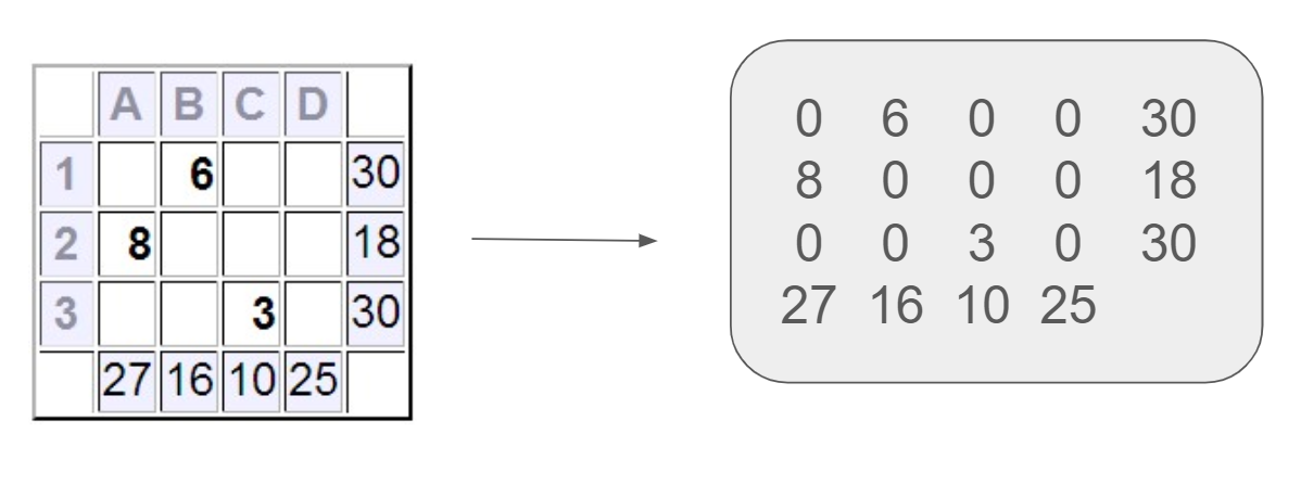
### Visual Description
## Diagram: Transformation of a Sparse Grid to a Dense Matrix
### Overview
The image displays a two-part diagram illustrating the transformation of a sparse, labeled grid (left) into a dense numerical matrix (right). An arrow points from the left grid to the right matrix, indicating a direct mapping or conversion process. This diagram is characteristic of representations used in operations research, specifically for formulating transportation or assignment problems.
### Components/Axes
**Left Component: Sparse Grid with Totals**
* **Structure:** A 3-row by 4-column grid.
* **Row Labels (Vertical Axis):** `1`, `2`, `3` (positioned to the left of each row).
* **Column Labels (Horizontal Axis):** `A`, `B`, `C`, `D` (positioned above each column).
* **Filled Cells (Data Points):**
* Cell at intersection of Row `1`, Column `B`: `6`
* Cell at intersection of Row `2`, Column `A`: `8`
* Cell at intersection of Row `3`, Column `C`: `3`
* **Row Totals (Right of Grid):** A column of numbers aligned with each row.
* Row `1` total: `30`
* Row `2` total: `18`
* Row `3` total: `30`
* **Column Totals (Below Grid):** A row of numbers aligned with each column.
* Column `A` total: `27`
* Column `B` total: `16`
* Column `C` total: `10`
* Column `D` total: `25`
**Right Component: Dense Matrix**
* **Structure:** A 4-row by 5-column matrix contained within a rounded rectangle.
* **Content (Row-wise):**
* **Row 1:** `0`, `6`, `0`, `0`, `30`
* **Row 2:** `8`, `0`, `0`, `0`, `18`
* **Row 3:** `0`, `0`, `3`, `0`, `30`
* **Row 4:** `27`, `16`, `10`, `25` (Note: This row contains only four values, aligned under the first four columns).
**Connector:** A simple right-pointing arrow (`→`) links the two components, indicating the direction of transformation.
### Detailed Analysis
The transformation maps the sparse grid and its marginal totals into a single, consolidated matrix.
1. **Mapping of Grid Values:** The non-zero values from the 3x4 grid (`6`, `8`, `3`) are placed into the first three rows and first four columns of the dense matrix at their corresponding (row, column) positions. All other cells in this 3x4 sub-matrix are filled with `0`.
2. **Incorporation of Row Totals:** The row totals (`30`, `18`, `30`) from the left are placed as the fifth element in the first three rows of the dense matrix.
3. **Incorporation of Column Totals:** The column totals (`27`, `16`, `10`, `25`) from the left are placed as the fourth row of the dense matrix, occupying the first four columns. The fifth column of this fourth row is empty/absent in the visual representation.
4. **Data Consistency Check:** The sum of the row totals (30 + 18 + 30 = 78) equals the sum of the column totals (27 + 16 + 10 + 25 = 78), indicating a balanced system, which is a fundamental requirement for a feasible solution in a transportation problem.
### Key Observations
* **Sparsity to Density:** The left grid is sparse (only 3 of 12 cells filled), while the right matrix is dense, with zeros explicitly shown.
* **Structural Transformation:** The diagram converts a "tableau" view with separate marginal totals into a unified matrix format where totals are integrated as an additional row and column.
* **Visual Anomaly:** The fourth row of the dense matrix has only four entries, breaking the rectangular pattern. This visually emphasizes that the column totals correspond only to the original four columns (A-D).
### Interpretation
This diagram almost certainly illustrates the **initial setup for a Transportation Problem** in linear programming or operations research.
* **Left Grid:** Represents the **cost matrix** or **initial allocation matrix**. The numbers `6`, `8`, `3` likely represent the cost per unit to ship from a source (rows 1,2,3) to a destination (columns A,B,C,D), or possibly an initial feasible allocation of units. The row totals (`30`, `18`, `30`) represent the **supply** at each source, and the column totals (`27`, `16`, `10`, `25`) represent the **demand** at each destination.
* **Right Matrix:** Represents the **standard tableau form** used in the Transportation Simplex Method (or similar algorithms). In this tableau:
* The top-left 3x4 block holds the unit costs or allocations.
* The fifth column holds the supply values.
* The fourth row holds the demand values.
* The bottom-right cell (implied but not shown) would typically hold the total cost or serve as a pivot point.
* **Purpose of Transformation:** Converting the problem into this dense matrix format allows for systematic application of algorithms (like the Northwest Corner Rule, Least Cost Method, or Vogel's Approximation Method) to find an initial basic feasible solution, which is then optimized. The zeros represent non-basic variables (routes not used in the initial solution).
The diagram serves as a clear visual guide for how to structure problem data from a descriptive format into a computational format ready for algorithmic solving.
</details>
Figure 10: Representation of input instances of survo as text.
Figure 10 represents the conversion of the inputs to survo, originally represented as grid images to text. Here empty cells are denoted by 0’s and the filled cells have corresponding values. For a given $m× n$ board, each row has $m+1$ space separated integers with the first m integers representing the first row of the input board and the $(m+1)^th$ integer representing the row sum. The last row contains $n$ integers represent the column sums. The box below describes this conversion more formally in natural language.
Input Format: - The input will have $m+1$ lines - The first $m$ lines will have $n+1$ space-separated integers - Each of these $m$ lines represents one row of the partially solved input board (n integers), followed by the required row sum (a single integer) - The last line of the input will have $n$ space-separated integers each of which represents the required column sum in the solved board Sample Input: 0 6 0 0 0 30 8 1 0 0 0 17 0 9 3 0 30 27 16 10 25
Output Format: - The output should have $m$ lines, each representing one row of the solved board - Each of these $m$ lines should have $n$ space-separated integers representing the cells of the solved board - Each integer should be from $1$ to $m*n$ Sample Output: 12 6 2 10 8 1 5 4 7 9 3 11
#### A.3.2 Example Problem: Dosun Fuwari
<details>
<summary>extracted/6211530/Images/dosun-fuwari-input-representation.png Details</summary>
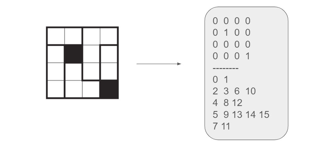
### Visual Description
## Diagram: Grid to Data Structure Transformation
### Overview
The image displays a two-part diagram illustrating a transformation from a visual grid representation to a structured numerical data format. On the left is a 4x4 grid with specific cells filled in black. An arrow points to the right, leading to a rounded rectangular container holding two distinct sets of numerical data separated by a dashed line. The diagram visually explains how a spatial or binary pattern is encoded into a hierarchical or indexed data structure.
### Components/Axes
1. **Left Component (Source Grid):**
* A 4x4 grid with uneven internal borders, creating a non-uniform cell structure.
* Two cells are filled with solid black.
* **Black Cell Positions (approximate):** Row 2, Column 2 and Row 4, Column 4 (assuming 1-based indexing from top-left).
2. **Transformation Indicator:**
* A simple right-pointing arrow (`→`) connects the left grid to the right data container, indicating a mapping or conversion process.
3. **Right Component (Data Container):**
* A light gray, rounded rectangle containing text.
* The content is divided into two sections by a horizontal dashed line (`---------`).
* **Top Section (Binary Matrix):** A 4x4 matrix of binary digits (0s and 1s).
* **Bottom Section (Indexed Lists):** Five rows of integers, with a varying number of entries per row.
### Detailed Analysis
**Top Section - Binary Matrix Transcription:**
```
0 0 0 0
0 1 0 0
0 0 0 0
0 0 0 1
```
* **Trend/Pattern:** This matrix is a direct binary representation of the left grid. A '1' corresponds to a black cell, and a '0' corresponds to a white cell. The '1's are located at positions (2,2) and (4,4), perfectly matching the visual grid.
**Bottom Section - Indexed Lists Transcription:**
```
0 1
2 3 6 10
4 8 12
5 9 13 14 15
7 11
```
* **Content:** This section contains the integers from 0 to 15, partitioned into five groups.
* **Spatial Grounding:** The numbers are arranged in a left-aligned list format within the container, below the dashed line.
* **Observation:** The grouping does not follow a simple sequential order. The numbers 5 and 15 (which correspond to the positions of the '1's in the binary matrix if cells are numbered 0-15 in row-major order) appear together in the fourth row of this list.
### Key Observations
1. **Direct Mapping:** The top numerical section is an exact binary encoding of the visual grid pattern.
2. **Non-Sequential Grouping:** The bottom section's grouping of numbers (0-15) is not sequential, suggesting it represents a specific traversal order, hierarchical decomposition (like a quadtree), or clustering based on the grid's structure.
3. **Structural Emphasis:** The thicker borders in the left grid may indicate a hierarchical subdivision (e.g., dividing the 4x4 grid into four 2x2 quadrants), which could be related to the grouping logic in the bottom list.
### Interpretation
This diagram demonstrates a method for converting a 2D spatial pattern (the grid) into a compact, structured data representation. The process involves two key steps:
1. **Binary Encoding:** First, the visual pattern is translated into a standard binary matrix, which is a fundamental format for digital image representation and processing.
2. **Structural Indexing:** Second, the cells of the grid are assigned unique indices (0-15) and then grouped into a specific, non-sequential order. This grouping likely reflects an underlying **spatial indexing scheme** or **hierarchical data structure**. Common examples include:
* **Quadtree Decomposition:** The grid is recursively divided into quadrants. The list order might represent a depth-first traversal of the quadtree nodes.
* **Space-Filling Curve (e.g., Z-order/Morton order):** The indices follow a path that preserves spatial locality, which is useful for efficient range queries in databases or image compression.
* **Run-Length Encoding (RLE) Variant:** The groups could represent runs of similar cells (e.g., background vs. foreground), though the presence of all numbers 0-15 makes this less likely.
**The core purpose** of the diagram is to illustrate how spatial information is abstracted and organized for computational efficiency. The black cells (data points of interest) are embedded within a larger structure, and the bottom list shows how all elements of that structure are cataloged in a specific, meaningful order that likely optimizes for operations like searching, compression, or spatial analysis. The transformation moves from a human-visual format to a machine-optimized format.
</details>
Figure 11: Representation of inputs instances to dosun-fuwari as text.
Figure 11 represents conversion of the inputs to dosun fuwari, originally represented as grid images to text. Here the first few lines represent the input board followed by a string ’—–’ which acts as a separator following which each of the lines has space-separated integers representing the subgrids of the input board. Cells are numbered in row-major order starting from 0, and this numbering is used to represent cells in each of the lines describing the subgrids. In the first few lines representing the input board, 0’s represent the empty cells that must be filled. 1’s denote the blackened cell, 2s denote the balloons and 3’s denote the iron balls. The box below describes these rules more formally in natural language
Input-Format: - The first few lines represent the input board, followed by a line containing --------, which acts as a separator, followed by several lines where each line represents one subgrid - Each of the lines representing the input board will have space-separated integers ranging from 0 to 3 - 0 denotes empty cells, 1 denotes a filled cell (blackened cell), 2 denotes a cell with a balloon, 3 denotes a cell with an iron ball - After the board, there is a separator line containing -------- - Each of the following lines has space-separated elements representing the subgrids on the input board - Each of these lines has integers representing cells of a subgrid - Cells are numbered in row-major order starting from 0, and this numbering is used to represent cells in each of the lines describing the subgrids Sample-Input: 0 0 0 0 0 1 0 0 0 0 0 0 0 0 0 1 -------- 0 1 2 3 6 10 4 8 12 5 9 13 14 15 7 11 Output Format: - The output should contain as many lines as the size of the input board, each representing one row of the solved board - Each row should have n space separate integers (ranging from 0-3) where n is the size of the input board - Empty cells will be denoted by 0s, filled cells (blackened) by 1s, balloons by 2s and iron balls by 3s Sample-Output: 2 3 0 2 2 1 0 2 0 2 3 3 3 0 3 1
#### A.3.3 Example Problem: Hamiltonian Path
<details>
<summary>extracted/6211530/Images/hamiltonian-path-input-representation.png Details</summary>
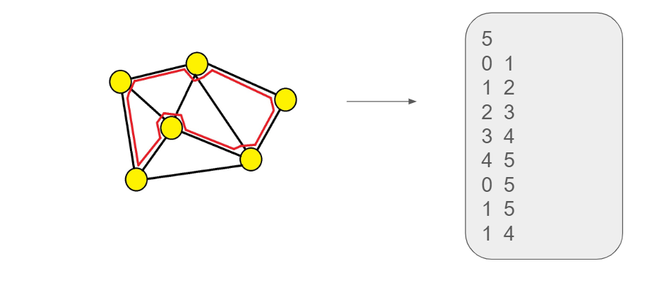
### Visual Description
## Diagram: Graph to Edge List Representation
### Overview
The image displays a diagram illustrating the conversion of a visual graph representation into a textual data structure, specifically an edge list. On the left is a planar graph with six nodes and eight edges. An arrow points to the right, where the graph's connectivity is encoded as a list of numerical pairs within a rounded rectangular container.
### Components/Axes
**Left Component (Graph):**
- **Nodes:** Six yellow circular nodes. They are unlabeled in the visual diagram but are inferred to represent vertices numbered 0 through 5 based on the accompanying list.
- **Edges:** Lines connecting the nodes exist in two colors:
- **Red Edges:** Form a closed cycle connecting all six nodes in sequence.
- **Black Edges:** Provide additional connections between nodes that are not adjacent in the red cycle.
- **Spatial Layout:** The graph is drawn in a roughly hexagonal arrangement with one central node. The red cycle forms the outer perimeter, and the black edges are internal chords.
**Right Component (Data List):**
- **Container:** A light gray, vertically oriented rectangle with rounded corners.
- **Content:** A list of numbers in a monospaced font. The first line contains a single number, followed by eight lines each containing a pair of numbers.
- **Arrow:** A simple black arrow points from the graph to the list, indicating a transformation or mapping process.
### Detailed Analysis
**Graph Structure (Inferred from List):**
The list provides the explicit edge data for the graph. The first number, `5`, likely indicates the maximum node index (implying nodes are labeled 0, 1, 2, 3, 4, 5). The subsequent pairs define the edges:
1. `0 1`
2. `1 2`
3. `2 3`
4. `3 4`
5. `4 5`
6. `0 5`
7. `1 5`
8. `1 4`
**Visual-to-Data Mapping:**
- The **red edges** in the diagram correspond to the cycle: `0-1`, `1-2`, `2-3`, `3-4`, `4-5`, and `5-0` (listed as `0 5`).
- The **black edges** correspond to the chords: `1-5` and `1-4`.
**Transcribed Text from List:**
```
5
0 1
1 2
2 3
3 4
4 5
0 5
1 5
1 4
```
### Key Observations
1. **Graph Type:** The graph is a **wheel graph** variant. It consists of a cycle (the red perimeter) with an additional central node (inferred to be node 1) connected to multiple other nodes.
2. **Node Degree:** Based on the edge list, node 1 has the highest degree (4 connections: to nodes 0, 2, 4, and 5). All other nodes have a degree of 3.
3. **Planarity:** The graph is drawn without any edge crossings, confirming it is a planar graph.
4. **Data Encoding:** The list is a standard **edge list** representation, a common format for storing graph data in computer science. The leading `5` is a metadata element specifying the vertex count or index range.
### Interpretation
This diagram serves as an educational or technical illustration of **graph representation**. It demonstrates the fundamental concept of translating a visual, abstract structure (a network of relationships) into a concrete, machine-readable format (a list of pairs).
The specific graph shown is not arbitrary; its structure—a cycle with chords—is common in network design, circuit layouts, and social network analysis. The red highlighting of the cycle emphasizes a primary pathway or loop within the system, while the black chords represent shortcuts or alternative connections. The transformation arrow underscores the critical process of **abstraction** in computer science, where visual models are converted into data structures for algorithmic processing, storage, and analysis. The presence of the leading `5` in the list also highlights the importance of metadata in defining the scope of the data (the set of nodes involved).
</details>
Figure 12: Representation of input instances to hamiltonian-path as text.
Figure 12 represents the conversion of inputs to hamiltonian-path, originally represented as graph image to text. The first line denotes the number of vertices present in the graph followed by which each node of the graph will be numbered from 0 - N-1. Each of the subsequent lines represents an edge of the graph and will contain two space-separated integers (according to the numbering defined previously). The output is a single word (YES/NO) indicating if a hamiltonian path exists in the graph. The box below describes this more formally in natural language.
Input Format: - The first line will contain a single integer N, the number of nodes in the graph - The nodes of the graph will be numbered from 0 to N-1 - Each of the subsequent lines will represent an edge of the graph and will contain two space-separated integers (according to the numbering defined above) Sample-Input: 5 0 1 1 2 2 3 3 4 Output Format: - The output should contain a single line with a single word - The word should be YES if a path exists in the input graph according to constraints specified above and NO otherwise Sample Output: YES
Table 7: Names of problems in FCoReBench, number of samples in the training set, number of samples in the test set, average size of input instances in training set, average size of input instances in test set and computational complexity. The brackets in the 4th column describe how input instance sizes are measured. ? in the computational complexity column indicates that results are not available for the corresponding problem.
| 3-Partition (Non Decision) | 15 | 30 | 12 (array size) | 17.7 | NP-Hard |
| --- | --- | --- | --- | --- | --- |
| 3-Partition (Decision) | 15 | 30 | 12 (array size) | 17.7 | NP-Complete |
| Binario | 15 | 50 | 4.0 $×$ 4.0 (grid size) | 6.96 $×$ 6.96 | NP-Hard [De Biasi, 2013] |
| Car-Sequencing | 15 | 30 | 6.96, 3.66, 4.33 (# of cars, # of options, # of classes) | 9.06, 5.66, 6.33 | NP-Hard [Kis, 2004] |
| Clique Cover | 15 | 30 | 6.26, 9.4 (# of nodes, # of edges) | 12.9, 31.4 | NP-Complete |
| Cryptarithmetic | 15 | 30 | 4.32 (Average # of digits in the two operands ) | 4.26 | NP-Hard [Epstein, 1987] |
| Dosun Fuwari | 15 | 30 | 3.066 $×$ 3.066 (grid size) | 5.23 $×$ 5.23 | NP-Hard [Iwamoto and Ibusuki, 2018] |
| Futoshiki | 15 | 47 | 5 $×$ 5 (grid size) | 7.57 $×$ 7.57 | NP-Hard [Lloyd et al., 2022] |
| Fill-a-pix | 15 | 35 | $2.87× 2.87$ (grid size) | $4.1× 4.1$ | NP-Hard [HIGUCHI and KIMURA, 2019] |
| Flow-Shop | 15 | 30 | 6.06, 3.4 (# of jobs, #num of machines) | 3.83, 9.13 | NP-Complete [Garey et al., 1976a] |
| Factory Workers | 15 | 30 | 5.73, 12.66 (# of factories, # of workers) | 12.35, 30.0 | ? |
| Graph Coloring | 15 | 30 | 5.13, 6.8 (# of nodes, # of edges) | 9, 21.06 | NP-Complete [Gent et al., 2017] |
| Hamiltonian Path | 15 | 30 | 5.93, 8.6 (# of nodes, # of edges) | 13.0, 19.77 | NP-Complete |
| Hamiltonian Cycle | 15 | 30 | 5.93, 8.6 (# of nodes, # of edges) | 11.07, 18.67 | NP-Complete |
| Hidato | 15 | 45 | $2.87× 2.87$ (grid size) | $4.1× 4.1$ | NP-Hard [Itai et al., 1982] |
| Independent Set | 12 | 30 | 5.8, 7.2 (# of nodes, # of edges) | 14.2, 29.8 | NP-Complete |
| Inshi-No-Heya | 15 | 49 | 5.0 $×$ 5.0 (grid size) | 6.5 $×$ 6.5 | ? |
| Job-Shop | 15 | 30 | 3.66, 3.66 (# of jobs, # of machines) | 9, 9 | NP-Complete [Garey et al., 1976b] |
| K-Clique | 15 | 31 | 4.87, 7.6 (# of nodes, # of edges) | 8.84, 26.97 | NP-Complete |
| Keisuke | 15 | 30 | 4.33 $×$ 4.33 (grid size) | 5.83 $×$ 5.83 | ? |
| Ken Ken | 15 | 20 | 3.26 $×$ 3.26 (grid size) | 5.2 $×$ 5.2 | NP-Hard [Haraguchi and Ono, 2015] |
| Knapsack | 15 | 30 | 4.8 (array size) | 24.56 | NP-Hard |
| K Metric Centre | 15 | 30 | 4.5 (# of nodes) | 7 | NP-Hard |
| Latin Square | 15 | 50 | 6 $×$ 6.0 (grid size) | 14.3 $×$ 14.3 | NP-Hard [Colbourn, 1984] |
| Longest Path Problem | 15 | 30 | 6.2, 5.87 (# of nodes, # of edges) | 12.6, 16.3 | NP-Complete |
| Magic Square | 15 | 30 | 3.0 $×$ 3.0 (grid size) | 4.33 $×$ 4.33 | ? |
| Minimum Dominating Set | 15 | 30 | 6.0, 17.73 (# of nodes, # of edges) | 14.53, 45.0 | NP-Complete |
| N-Queens | 15 | 30 | 3.8 $×$ 3.8 (grid size) | 6.33 $×$ 6.33 | NP-Hard [Gent et al., 2017] |
| Number Link | 15 | 50 | 4 $×$ 4 (grid size) | 7.1 $×$ 7.1 | NP-Hard |
| Partition Problem | 15 | 35 | 7.06 (array size) | 15 | NP-Complete |
| PRP | 15 | 30 | 4.93, 12.6 (# of units, # of days) | 6.7, 23.9 | ? |
| Shinro | 15 | 30 | 5.13 $×$ 5.13 (grid size) | 9.2 $×$ 9.2 | ? |
| Subset Sum | 15 | 30 | 3.67 (array size) | 11.87 | NP-Complete |
| Summle | 15 | 20 | 2.33 (# of equations) | 3.75 | ? |
| Sudoku | 15 | 50 | 4.0 $×$ 4.0 (grid size) | 13.3 $×$ 13.3 | NP-Hard [YATO and SETA, 2003] |
| Sujiko | 15 | 45 | 3.0 $×$ 3.0 (grid size) | 4.0 $×$ 4.0 | ? |
| Survo | 15 | 47 | 13.5 (area of grid) | 20.25 | ? |
| Symmetric Sudoku | 15 | 30 | 4 $×$ 4 (grid size) | 6.5 $×$ 6.5 | ? |
| Sliding Tiles | 15 | 30 | $2.66× 2.66$ , 6.13 (grid size, search depth) | $3.63× 3.63$ , 8.83 | NP-Complete [Demaine and Rudoy, 2018] |
| Vertex Cover | 14 | 30 | 6.4, 13.4 (# of nodes, # of edges) | 12.6, 40.4 | NP-Complete |
## Appendix B Prompt Templates
In this section we provide prompt templates used for our experiments on FCoReBench, including the templates for the baselines we experimented with, SymPro-LM as well as prompt templates for providing feedback.
### B.1 Few-Shot Prompt Template
Task: <Description of the Rules of the problems>
Input-Format: <Description of Textual Representation of Inputs> <Input Few Shot Example-1> <Input Few Shot Example-2> ........................ ........................ <Input Few Shot Example-n>
Output-Format
<Description of Textual Representation of Outputs> <Output of Few Shot Example-1> <Output of Few Shot Example-2> ............................ ............................ <Output of Few Shot Example-n>
Input problem instance to be solved: <Problem Instance from the Test Set>
### B.2 PAL Prompt Template
The following box describes the base prompt template used for PAL experiments with FCoReBench.
Write a Python program to solve the following problem: Task: <Description of the Rules of the problem> Input-Format: <Description of Textual Representation of Inputs> Sample-Input: <Sample Input from Feedback Set> Output-Format: <Description of Textual Representation of Outputs> Sample-Output: <Output of Sample Input from Feedback Set> Don’t write anything apart from the Python program; use Python comments if needed. The Python program is expected to read the input from input.txt and write the output to a file named output.txt. The Python program must only use standard Python libraries.
### B.3 SymPro-LM Template
#### B.3.1 Base Prompt
Write a Python program to solve the following problem: Task: <Description of the Rules of the problem>
Input-Format: <Description of Textual Representation of Inputs> Sample-Input: <Sample Input from Feedback Set>
Output-Format: <Description of Textual Representation of Outputs> Sample-Output: <Output of Sample Input from Feedback Set>
The Python program must read the input from input.txt and convert that particular input to the corresponding constraints, which it should pass to the Z3 solver, and then it should use the Z3 solver’s output to write the solution to a file named output.txt
Don’t write anything apart from the Python program; use Python comments if needed.
### B.4 Feedback Prompt Templates
These prompt templates are used to provide feedback in the case of SymPro-LM or PAL.
#### B.4.1 Programming Errors
Your code is incorrect and produces the following runtime error:<RUN TIME ERROR> for the following input: <INPUT> rewrite your code and fix the mistake
#### B.4.2 Verification Error
Your code is incorrect, when run on the input: <INPUT> the output produced is <OUTPUT-GENERATED> which is incorrect whereas one of the correct output is <GOLD-OUTPUT>. Rewrite your code and fix the mistake.
#### B.4.3 Timeout Error
Your code was inefficient and took more than <TIME-LIMIT> seconds to execute for the following input: <INPUT>. Rewrite the code and optimize it.
### B.5 Logic-LM Prompt Template
The following box describes the prompt for Logic-LM experiments with FCoReBench, the prompt is used to convert the input to its symbolic representation.
Task: <Description of the Rules of the problem> Input-Format: <Description of Textual Representation of Inputs> Sample-Input: <Sample Input from Feedback Set> Output-Format: <Description of Textual Representation of Outputs> Sample-Output: <Output of Sample Input from Feedback Set> Input problem to be solved: <Problem Instance from the Test Set> The task is to declare variables and the corresponding constraints on them in SMT2 for the input mentioned above. The variables and constraints should be such that once the variables are solved for, one can use the solution to the variables (which satisfies the constraints) to get to the output in the desired format for the above mentioned input. Only Write the SMT2 code and nothing else. Write the complete set of SMT2 variables and constraints. Enclose SMT2 code in ‘‘‘smt2 ‘‘‘
### B.6 ToT
In this section we give an example of the ToT prompts used for experiments on FCoReBench. We use latin square as the running example.
#### B.6.1 Propose Prompt
This prompt is called for each search node to get the possible next states.
Task: We are given a nxn partially solved board and have to solve it according to the following rules: - We need to replace the 0s with numbers from 1-n. - Non-zero numbers on the board cannot be replaced. - Each number from 1-n must appear exactly once in each column and row in the solved board Given a board, decide which cell to fill in next and the number to fill it with, each possible next step is separated by a new line. You can output up-to 3 next steps. If the input board is fully filled or no valid next step exists output only ’END’. Sample-Input-1: 1 0 3 2 0 0 0 1 2 Possible next steps for Sample Input-1: 1 2 3 2 0 0 0 1 2 1 0 3 2 0 0 3 1 2 1 0 3 2 3 0 0 1 2 Sample-Input-2: 1 2 3 2 3 1 3 1 2 Possible next steps for Sample Input-2: END Input: <node from the search tree> Possible next steps for Input:
#### B.6.2 Value Prompt
This prompt is called for each search node to evaluate how likely it is to get to the solution from that node. We use this to prune the search tree.
Task: We are given a nxn partially solved board and have to solve it according to the following rules: - We need to replace the 0s with numbers from 1-n. - Non-zero numbers already on the board cannot be replaced. - Each number from 1-n must appear exactly once in each column and row in the solved board. Given a partially filled board, evaluate how likely it is to reach a valid solution (sure/likely/impossible) Output-Format: The output should have two lines as follows: <Reasoning> <Sure/Likely/Impossible> Sample-Input-1: 0 0 0 0 0 0 0 0 0 Board is empty, hence it is always possible to get to a solution. Sure Sample-Input-2: 1 0 3 2 0 0 0 1 2 No constraint is violated till now and it is likely to get to a solution. Likely Sample-Input-3: 1 1 3 2 0 0 0 1 2 Constraint violated in first row. Impossible Input: <node from the search tree>
## Appendix C Experimental Details
### C.1 FCoReBench
All methods are evaluated zero-shot, meaning no in-context demonstrations for the task are provided to the LLM. We choose the zero-shot setting for FCoReBench because of the structured nature of problems, making it unfair to provide demonstrations of highly related problems instances to the LLM. The LLM is only given a description of the rules of the problem and the task it has to perform. For PAL and SymPro-LM we present results with 10 solved examples for feedback.
#### C.1.1 ToT prompting
We evaluate ToT prompting [Yao et al., 2023] on 3 problems in FCoReBench. Our implementation closely resembles the official implementation which we adapt for grid based logical puzzles. We use a BFS based approach with propose and value prompts. An example prompt for latin square can be found in Appendix B.6. Problems in our benchmark have huge branching factors, to reduce experimentation cost, we greedily prune the search frontier to 5 nodes at each depth based on scores assigned by the LLM during the value stage. Additionally during the propose stage we prompt the LLM to output at most 3 possible next steps. The temperature is set to 0.0 for reproducibility. Unlike the original implementation problems in our benchmark can have varying search depths, hence we explicitly ask the LLM to output ’END’ once a terminal node is reached. At any depth if a terminal node is amongst the best nodes we terminate the search and return the terminal nodes at that depth, otherwise we search till a maximum search depth governed by the problem instance.
### C.2 Other Datasets
We evaluate SymPro-LM on 3 other datasets apart from FCoReBench. Our evaluation closely follows Logic-LM’s evaluation [Pan et al., 2023]. For baselines we use the same prompts as Logic-LM. Logic-LM did not evaluate PAL, for which we write prompts on our own similar to the CoT prompts used by Logic-LM. For SymPro-LM we write prompts on our own. We use the same in-context examples as used for Logic-LM. We instruct the LLM to write a Python program to parse the input problem, setup variables/constraints and pass these to a symbolic solver, call the solver and using the solver’s output print the final answer. For LogicalDeduction we use the python-constraints https://github.com/python-constraint/python-constraint package which is a CSP solver. For other datasets we use the Z3-solver https://pypi.org/project/z3-solver/. Since all problems are single correct MCQ questions we use accuracy as our metric. Like Logic-LM if there is an error during execution of the program generated by the LLM we fall back on using chain-of-thought to predict the answer. The following sections provide descriptions for the datasets used.
#### C.2.1 PrOntoQA
PrOntoQA [Saparov and He, 2023a] is a recent synthetic dataset created to analyze the deductive reasoning capacity of LLMs. We use the hardest fictional characters version of the dataset, based on the results in [Saparov and He, 2023a]. Each version is divided into different subsets depending on the number of reasoning hops required. We use the hardest 5-hop subset for evaluation. Each question in PrOntoQA aims to validate a new fact’s veracity, such as “True or false: Alex is not shy.” The following box provides an example:
Context: Each jompus is fruity. Every jompus is a wumpus. Every wumpus is not transparent. Wumpuses are tumpuses. Tumpuses are mean. Tumpuses are vumpuses. Every vumpus is cold. Each vumpus is a yumpus. Yumpuses are orange. Yumpuses are numpuses. Numpuses are dull. Each numpus is a dumpus. Every dumpus is not shy. Impuses are shy. Dumpuses are rompuses. Each rompus is liquid. Rompuses are zumpuses. Alex is a tumpus Question: True or false: Alex is not shy. Options: A) True B) False
#### C.2.2 ProofWriter
ProofWriter [Tafjord et al., 2021] is another commonly used dataset for deductive logical reasoning. Compared with PrOntoQA, the problems are expressed in a more naturalistic language form. We use the open-world assumption (OWA) subset in which each example is a (problem, goal) pair and the label is one of PROVED, DISPROVED, UNKNOWN. The dataset is divided into five parts each part requiring 0, $≤$ 1, $≤$ 2, $≤$ 3, and $≤$ 5 hops of reasoning, respectively. We evaluate the hardest depth-5 subset. To reduce overall experimentation costs, we randomly sample 600 examples in the test set and ensure a balanced label distribution. The following box provides an example:
Context: Anne is quiet. Erin is furry. Erin is green. Fiona is furry. Fiona is quiet. Fiona is red. Fiona is rough. Fiona is white. Harry is furry. Harry is quiet. Harry is white. Young people are furry. If Anne is quiet then Anne is red. Young, green people are rough. If someone is green then they are white. If someone is furry and quiet then they are white. If someone is young and white then they are rough. All red people are young. Question: Based on the above information, is the following statement true, false, or unknown? Anne is white. Options: A) True B) False C) Uncertain
#### C.2.3 LogicalDeduction
LogicalDeduction bench authors, 2023 is a challenging logical reasoning task from the BigBench collaborative benchmark. The problems are mostly about deducing the order of a sequence of objects from a minimal set of conditions. We use the full test set consisting of 300 examples. The following box provides an example:
Context: The following paragraphs each describe a set of three objects arranged in a fixed order. The statements are logically consistent within each paragraph. In an antique car show, there are three vehicles: a station wagon, a convertible, and a minivan. The station wagon is the oldest. The minivan is newer than the convertible. Question: Which of the following is true? Options: A) The station wagon is the second-newest. B) The convertible is the second-newest. C) The minivan is the second-newest.
### C.3 Hardware Details
All experiments were conducted on an Intel(R) Xeon(R) Gold 6226R CPU @ 2.90GHz, 32 cores, 64-bit, with 512 KiB L1 cache, 16 MiB L2 cache, and 22 MiB L3 cache. We accessed GPT-4-Turbo and GPT-3.5-Turbo by invoking both models via the OpenAI API. Mixtral 8x7B was also accessed by using the Mistral AI API although the model weights are available publicly. We preferred the API, over running the model locally given the ease of setup because all our other experiments were with APIs.
## Appendix D Additional Results
### D.1 Inference Time
The following tables describes the average inference time for test set instances of a few illustrative problems in FCoReBench.
| Sudoku Latin Square Cryptarithmetic | 2.01 5.46 0.83 | 0.215 0.2 0.73 |
| --- | --- | --- |
| Independent Set | 1.438 | 0.106 |
| Minimum Dominating Set | 0.98 | 0.112 |
| Sujiko | 0.742 | 0.102 |
| Vertex Cover | 1.58 | 0.105 |
Table 8: Average inference time in seconds of SymPro-LM and PAL for test set instances for selected problems in FCoReBench
SymPro-LM performs much better compared to PAL because PAL programs often tend to be brute force and inefficient whereas the solver can exploit the nature of the input-instance while performing the reasoning with SymPro-LM.
## Appendix E Examples
### E.1 SymPro-LM
#### E.1.1 FCoReBench
This section includes example programs generated by SymPro-LM for some illustrative problems in FCoReBench. Each program reads the input from a file, generates the corresponding constraints, calls the solver internally and then uses the solution from the solver to write the output in the desired format to a file.
Figure 13: SymPro-LM example: correct program for sudoku generated by GPT-4-Turbo.
Figure 14: SymPro-LM example: correct program for keisuke generated by GPT-4-Turbo.
Figure 15: SymPro-LM example: correct program for hamiltonian path generated by GPT-4-Turbo.
Figure 16: SymPro-LM example: correct program for vertex-cover generated by GPT-4-Turbo.
Figure 17: SymPro-LM example: snippet of incorrect program for binairo generated by GPT-4-Turbo and same snippet after correction by feedback.
Figure 18: SymPro-LM example: correct program for subset-sum generated by GPT-4-Turbo.
#### E.1.2 Other Datasets
Figure 19: SymPro-LM PrOntaQA Example Program.
Figure 20: SymPro-LM ProofWriter Example Program.
Figure 21: SymPro-LM LogicalDeduction Example Program.
### E.2 PAL
This section includes example programs generated by PAL for some illustrative problems in FCoReBench. Each program reads the input from a file, performs the reasoning and writes the output to another text file.
Figure 22: PAL example: correct program for sudoku generated by GPT-4-Turbo.
Figure 23: PAL example: correct program for futoshiki generated by GPT-4-Turbo.
Figure 24: PAL example: correct program for hamiltonian path generated by GPT-4-Turbo.
Figure 25: PAL example: correct program for vertex cover generated by GPT-4-Turbo.
Figure 26: PAL example: correct program for subset sum generated by GPT-4-Turbo.
## Appendix F Logic-LM
This section describes example runs of Logic-LM for certain problems in FCoReBench.
Figure 27: Logic-LM example: correct constraints for a sudoku instance generated by GPT-4-Turbo.
Figure 28: Logic-LM example: correct constraints for a subset sum instance generated by GPT-4-Turbo.
Figure 29: Logic-LM example: correct constraints for graph coloring instance generated by GPT-4-Turbo.
Figure 30: Logic-LM example: syntax error (highlighted by a comment) in constraints for sudoku instance generated by GPT-3.5-Turbo.
Figure 31: Logic-LM example: errors (highlighted comments) in constraints for sudoku instance generated by GPT-4-Turbo.