2402.02834

# Shortened LLaMA: Depth Pruning for Large Language Models with Comparison of Retraining Methods > Equal contribution.Corresponding author. ## Abstract Structured pruning of modern large language models (LLMs) has emerged as a way of decreasing their high computational needs. Width pruning reduces the size of projection weight matrices (e.g., by removing attention heads) while maintaining the number of layers. Depth pruning, in contrast, removes entire layers or blocks, while keeping the size of the remaining weights unchanged. Most current research focuses on either width-only or a blend of width and depth pruning, with little comparative analysis between the two units (width vs. depth) concerning their impact on LLM inference efficiency. In this work, we show that simple depth pruning can effectively compress LLMs while achieving comparable or superior performance to recent width pruning studies. Our pruning method boosts inference speeds, especially under memory-constrained conditions that require limited batch sizes for running LLMs, where width pruning is ineffective. In retraining pruned models for quality recovery, continued pretraining on a large corpus markedly outperforms LoRA-based tuning, particularly at severe pruning ratios. We hope this work can help build compact yet capable LLMs. Shortened LLaMA: Depth Pruning for Large Language Models with Comparison of Retraining Methods Bo-Kyeong Kim 1 thanks: Equal contribution. Geonmin Kim 1 footnotemark: Tae-Ho Kim 1 thanks: Corresponding author. Thibault Castells 1 Shinkook Choi 1 Junho Shin 1 Hyoung-Kyu Song 2 1 Nota Inc. 2 Captions {bokyeong.kim, geonmin.kim, thkim, thibault, shinkook.choi, junho.shin}@nota.ai, kyu@captions.ai ## 1 Introduction The advancement of large language models (LLMs) Touvron et al. (2023); OpenAI (2023); Chowdhery et al. (2022); Zhang et al. (2022); Scao et al. (2022) has brought significant improvements in language-based tasks, enabling versatile applications such as powerful chatbots Google (2023); OpenAI (2022). However, the deployment of LLMs is constrained by their intensive computational demands. To make LLMs more accessible and efficient for practical use, various optimization strategies have been actively studied over recent years (see Zhu et al. (2023); Wan et al. (2023) for survey). This work focuses on structured pruning Fang et al. (2023); Li et al. (2017a), which removes groups of unnecessary weights and can facilitate hardware-agnostic acceleration. <details> <summary>x1.png Details</summary>  ### Visual Description ## [Chart Type: Multi-Panel Performance Analysis (Line Graph + Bar Graphs)] ### Overview The image contains three panels: a left line graph (Throughput vs. Latency) and two right bar graphs (Perplexity (PPL) and Accuracy (Acc) vs. Model Size). It compares the performance of different methods (Original, FLAP, LLM-Prn., Ours, SLEB, Ours-CPT) across metrics like throughput, latency, perplexity, and accuracy. ### Components/Axes #### Left Panel: Throughput vs. Latency (Line Graph) - **Y-axis**: Throughput (tokens/s) (logarithmic scale: 32, 64, 128, 256, 512, 1024, 2048, 4096, 8192). - **X-axis**: Latency (s) (linear scale: 1.6, 2.8, 4, 5.2, 6.4). - **Legend**: - Gray cross: *Original* - Green circle: *FLAP* - Green triangle: *LLM-Prn.* - Blue square: *Ours* - **Batch Sizes (M)**: Labeled on the *Ours* line: M1, M8, M16, M32, M64, M128, M256. - **Setup**: 4.9B Parameters, 12 Input Tokens, 128 Output Tokens (text at bottom). #### Right Top Panel: Perplexity (PPL) vs. Model Size (Bar Graph) - **Y-axis**: PPL (lower = better; values: 20, 30, 40; >40 omitted). - **X-axis**: Model Size (# Parameters: 5.5B, 3.7B, 2.7B). - **Legend (top-right)**: - Dark green: *FLAP (W%)* - Light green: *LLM-Prn. (W%)* - Light blue: *SLEB (D%)* - Dark blue: *Ours-CPT (D%)* #### Right Bottom Panel: Accuracy (Acc) vs. Model Size (Bar Graph) - **Y-axis**: Accuracy (%) (values: 40, 50, 60). - **X-axis**: Model Size (# Parameters: 5.5B, 3.7B, 2.7B). - **Legend (top-right)**: Same as PPL (FLAP, LLM-Prn., SLEB, Ours-CPT). ### Detailed Analysis #### Left Panel: Throughput vs. Latency - **Trends**: - *Ours* (blue squares) has the **highest throughput** across most latencies, especially at larger batch sizes (M128, M256). - *Original* (gray crosses) has lower throughput, increasing with latency but slower than *Ours*. - *FLAP* (green circles) and *LLM-Prn.* (green triangles) lie between *Original* and *Ours*, with *LLM-Prn.* slightly outperforming *FLAP* at some points. - **Key Data Points** (approximate): - *Ours* at M256: Throughput ~8192 tokens/s, Latency ~6.4s. - *Original* at M256: Throughput ~4096 tokens/s, Latency ~6.4s. #### Right Top Panel: Perplexity (PPL) - **Trends**: - *Ours-CPT* (dark blue) has the **lowest PPL** (best language modeling) across all model sizes. - *FLAP*, *LLM-Prn.*, and *SLEB* have higher PPL (worse performance), especially at 3.7B and 2.7B (exceeding 40 for some). - **Key Data Points** (approximate): - 5.5B: *Ours-CPT* ~15, *FLAP* ~22, *LLM-Prn.* ~20, *SLEB* ~25. - 3.7B: *Ours-CPT* ~15, *FLAP* ~40, *LLM-Prn.* ~40, *SLEB* ~40. #### Right Bottom Panel: Accuracy (Acc) - **Trends**: - *Ours-CPT* (dark blue) has the **highest accuracy** across all model sizes. - *SLEB* (light blue) has the lowest accuracy. *FLAP* and *LLM-Prn.* lie in between, with *LLM-Prn.* slightly outperforming *FLAP* at 3.7B and 2.7B. - **Key Data Points** (approximate): - 5.5B: *Ours-CPT* ~61%, *FLAP* ~61%, *LLM-Prn.* ~60%, *SLEB* ~55%. - 3.7B: *Ours-CPT* ~57%, *FLAP* ~47%, *LLM-Prn.* ~50%, *SLEB* ~40%. ### Key Observations - **Efficiency (Throughput/Latency)**: *Ours* outperforms *Original*, *FLAP*, and *LLM-Prn.* in throughput (tokens/s) at similar or lower latency, especially with larger batch sizes. - **Performance (PPL/Acc)**: *Ours-CPT* outperforms *FLAP*, *LLM-Prn.*, and *SLEB* in both perplexity (lower = better) and accuracy (higher = better) across all model sizes. - **Model Size Impact**: Larger models (5.5B) generally have better PPL and accuracy than smaller ones (3.7B, 2.7B), but *Ours-CPT* maintains strong performance even at 2.7B. ### Interpretation The data suggests that the “Ours” method (and its variant “Ours-CPT”) is more efficient (higher throughput, lower latency) and effective (lower PPL, higher accuracy) than competing methods (Original, FLAP, LLM-Prn., SLEB). This implies: - **Efficiency**: “Ours” processes more tokens per second with less delay, making it suitable for high-throughput applications. - **Effectiveness**: “Ours-CPT” achieves better language modeling (lower PPL) and task accuracy, indicating improved model quality. - **Scalability**: Performance gains hold across different model sizes (5.5B, 3.7B, 2.7B), suggesting the method scales well. These results highlight the superiority of “Ours” in both efficiency and performance, making it a promising approach for large language model optimization. 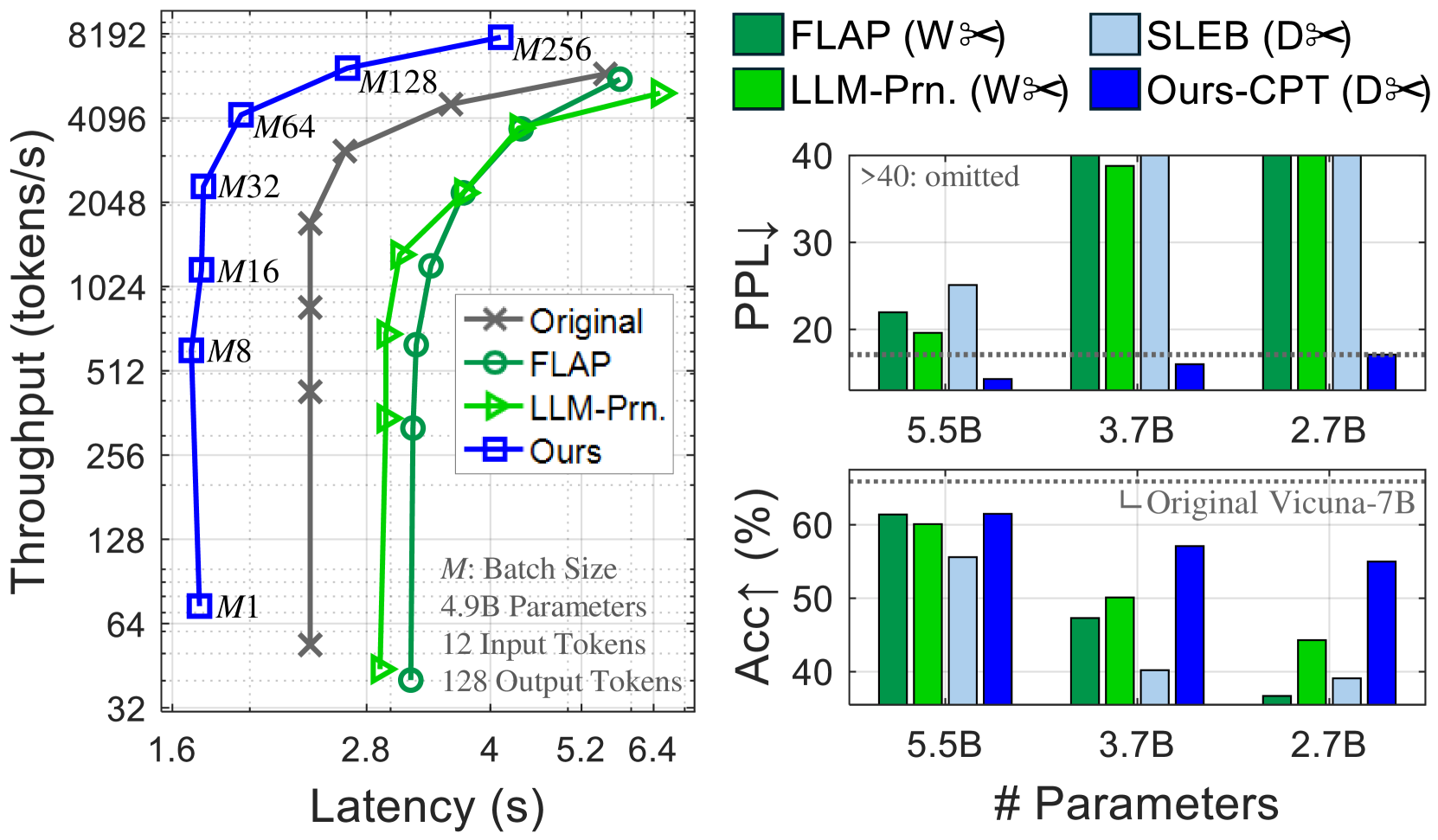</details> Figure 1: Inference of pruned Vicuna-7B models on an NVIDIA H100 GPU. Left: Compared to width pruning (W✂) of FLAP An et al. (2024) and LLM-Pruner Ma et al. (2023), our depth pruning (D✂) achieves faster inference. Right: Continued pretraining is crucial for restoring the quality of heavily pruned models with fewer than 3.7B parameters, enabling our method to surpass the baselines, including SLEB Song et al. (2024). See Table 3 for details. <details> <summary>x2.png Details</summary>  ### Visual Description ## [Composite Performance Analysis]: GPU Utilization and Latency for LLMs ### Overview The image is a composite of four subplots (a–d) analyzing GPU utilization (heatmaps, top) and latency (line graphs, bottom) for large language models (LLMs) across different GPUs (RTX3090, A100, H100), model sizes (7B, 13B), batch sizes, and sequence lengths. Each subplot includes a heatmap (utilization %) and two line graphs (latency in seconds) for sequence lengths \( L128 \) and \( L512 \). ### Components/Axes #### Heatmaps (Top of Each Subplot) - **Axes**: - *X-axis*: Batch Size (1, 2, 4, 8, 16, 32, 64, 128, 256, 384, 512). - *Y-axis*: Sequence Length (16, 32, 64, 128, 256, 512, 1024). - *Color Bar*: Utilization (%) (50 = yellow, 100 = red; “OOM” = Out of Memory, gray). - **Subplot Titles**: - (a) 7B’s RTX3090 Utilization [%] - (b) 7B’s A100 Utilization [%] - (c) 7B’s H100 Utilization [%] - (d) 13B’s H100 Utilization [%] #### Line Graphs (Bottom of Each Subplot) - **Axes**: - *X-axis*: Batch Size (1, 10, 100, 384) (logarithmic scale). - *Y-axis*: Latency (s) (varies per subplot). - **Legend**: - Gray: Original model - Green: Width×2 (model width scaled by 2) - Blue: Depth×2 (model depth scaled by 2) - **Subplot Titles (Line Graphs)**: - Left: \( L128 \) (Sequence Length = 128) - Right: \( L512 \) (Sequence Length = 512) ### Detailed Analysis #### Subplot (a): 7B’s RTX3090 Utilization - **Heatmap**: - Utilization increases with batch size and sequence length, but “OOM” occurs at high batch sizes (e.g., batch 512, seq 1024). - Key points: Seq 128, batch 128: 97% (purple box); Seq 512, batch 128: 91% (purple box). - **Line Graphs**: - \( L128 \): Latency rises with batch size (Original: ~4–8s; Width×2: ~5–9s; Depth×2: ~4–7s). - \( L512 \): Latency is higher (Original: ~22–30s; Width×2: ~22–30s; Depth×2: ~14–22s). #### Subplot (b): 7B’s A100 Utilization - **Heatmap**: - Higher utilization than RTX3090. Seq 128, batch 128: 100% (purple box); Seq 512, batch 128: 100% (purple box). - “OOM” at high batch sizes (e.g., batch 512, seq 1024). - **Line Graphs**: - \( L128 \): Latency lower than RTX3090 (Original: ~2–12s; Width×2: ~2–12s; Depth×2: ~2–12s, steeper at batch 384). - \( L512 \): Latency ~7–35s (all configurations, steeper at batch 384). #### Subplot (c): 7B’s H100 Utilization - **Heatmap**: - Utilization similar to A100. Seq 128, batch 128: 100% (purple box); Seq 512, batch 128: 99% (purple box). - “OOM” at high batch sizes. - **Line Graphs**: - \( L128 \): Latency ~2–6s (all configurations, steeper at batch 384). - \( L512 \): Latency ~7–19s (all configurations, steeper at batch 384). #### Subplot (d): 13B’s H100 Utilization - **Heatmap**: - Larger model (13B) on H100. Seq 128, batch 128: 99% (purple box); Seq 512, batch 128: 98% (purple box). - “OOM” at high batch sizes. - **Line Graphs**: - \( L128 \): Latency ~2–6s (all configurations, steeper at batch 384). - \( L512 \): Latency ~8–20s (all configurations, steeper at batch 384). ### Key Observations 1. **Utilization Trend**: GPU utilization increases with batch size and sequence length, but “OOM” occurs at high batch sizes (≥256) and sequence lengths (≥512). 2. **Latency Trend**: Latency rises with batch size, especially at larger sequence lengths (\( L512 > L128 \)). Width×2 and Depth×2 configurations have similar latency to the Original model. 3. **GPU Comparison**: A100 and H100 outperform RTX3090 in utilization for the 7B model. The 13B model on H100 has slightly lower utilization than the 7B model on H100. 4. **OOM Occurrence**: “OOM” is more frequent at high batch sizes (≥256) and sequence lengths (≥512) across all GPUs. ### Interpretation - **Utilization vs. Batch/Sequence**: Higher batch sizes and sequence lengths maximize GPU utilization (up to 100%) but risk “OOM,” highlighting a trade-off between utilization and memory constraints. - **Latency vs. Configuration**: Model scaling (Width×2, Depth×2) does not drastically increase latency, but batch size does. This suggests scaling model width/depth is feasible with manageable latency increases. - **GPU Performance**: A100 and H100’s higher utilization (vs. RTX3090) for the 7B model reflects their superior memory and compute capabilities. The 13B model’s slightly lower utilization on H100 may stem from higher memory demands. - **Practical Implications**: Balance batch size and sequence length to maximize utilization without “OOM.” Model scaling (Width×2, Depth×2) is viable for performance gains with minimal latency impact. This analysis provides a comprehensive view of GPU utilization and latency trade-offs for LLMs, enabling informed decisions on hardware, model scaling, and batch/sequence length optimization. 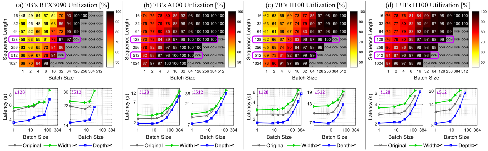</details> Figure 2: Top: GPU compute utilization of (a)–(c) running LLaMA-7B on different NVIDIA GPUs and that of (d) Vicuna-13B. Increasing batch sizes can enhance GPU utilization and throughput, but pushing this too far triggers OOM issues. Bottom: Latency results ( $L$ : target output length). Our depth pruning (blue lines) improves generation speeds over the original models (gray), while width pruning Ma et al. (2023) is ineffective (green). The dotted lines show that pruned models can operate with larger batch sizes that cause OOM errors for the original model. The results are obtained with pruning ratios of 27% for the 7B model and 29% for the 13B model. In the context of compressing recent LLMs, LLM-Pruner Ma et al. (2023) and FLAP An et al. (2024) narrow the network width by pruning coupled structures (e.g., attention heads and their associated weight connections) while maintaining the number of layers. Sheared-LLaMA Xia et al. (2024) reduces not only the network width but also its depth by entirely removing some layers. Despite the existence of pruning methods Xia et al. (2022); Kurtic et al. (2023); Xia et al. (2024) that incorporate both width and depth aspects, there remains a gap in detailed analysis comparing these two factors (width vs. depth), specifically in relation to their impact on LLM inference efficiency. In addition to substantial model sizes, LLM inference is distinguished by an autoregressive decoding mechanism, which predicts tokens one by one based on the input and the previously generated tokens. This sequential generation process often exhibits a memory-bound nature, leading to considerable underutilization of GPU compute abilities Kwon et al. (2023); Jin et al. (2023). While expanding batch sizes is a standard way to enhance GPU utilization and throughput, this approach is unfeasible for low-specification GPUs with memory constraints. We aim to improve inference speeds of LLMs, especially under hardware limitations that demand small batch sizes, where we observe that width-only pruning is inadequate. Depth pruning is often regarded as being less effective in generation performance compared to width pruning, due to the elimination of bigger and coarse units. Contrary to the prevailing view, this study reveals that depth pruning is a compelling option for compressing LLMs, and it can achieve comparable or superior performance to prior studies depending on the retraining setups. Our contributions are summarized as follows: 1. In scenarios with limited batch sizes, our work demonstrates that width pruning is difficult to attain actual speedups in LLM’s autoregressive generation. This aspect has been underexplored in previous works. 1. We introduce a simple yet effective method for depth pruning of LLMs by exploring various design factors. Our compact LLMs, obtained by excluding several Transformer blocks, achieve actual speedups. 1. We show that under moderate pruning ratios, our depth pruning method with LoRA retraining can rival recent width pruning studies for LLMs in zero-shot capabilities. For more aggressive pruning (over 40% removal), intensive retraining with a full-parameter update is crucial for recovering performance. <details> <summary>x3.png Details</summary>  ### Visual Description ## [Diagram]: Transformer Language Model with Depth and Width Pruning ### Overview The image is a technical diagram illustrating a **Transformer-based language model** architecture, with two model compression techniques: **Depth Pruning** (removing entire Transformer blocks) and **Width Pruning** (pruning components within a Transformer block). The left side shows the overall model structure, while the right side provides a detailed view of a single Transformer block’s internal components. ### Components/Axes (Diagram Elements) #### Left Side (Model Architecture) - **Input Embedding**: Feeds into the first Transformer block (`Transformer Block₁`). - **Transformer Blocks**: Stacked sequentially from `Transformer Block₁` to `Transformer Blockₙ`. - `Transformer Blockₙ` (top) connects to the **LM Head** (Language Model Head), which produces the **Output Logit**. - `Transformer Blockₙ₋₁` (middle) is highlighted with a blue dashed border and a **blue scissors icon** (labeled *Depth Pruning*), indicating pruning of entire blocks. - **Depth Pruning**: Blue scissors icon + label *“Depth Pruning”* (bottom-left) denotes removing entire Transformer blocks to reduce model depth. #### Right Side (Transformer Block Detail) - **Transformer Blockₙ₋₁** (connected to the left) is expanded to show internal components: - **MHA (Multi-Head Attention)**: - Contains `QKV₁`, `QKVₕ`, `QKVₕ` (likely `QKV₁` to `QKVₕ`, with a **green scissors icon** on `QKVₕ`, indicating pruning of attention heads). - Includes an *“Out”* (output) layer and a *“Norm”* (normalization) layer below MHA. - **FFN (Feed-Forward Network)**: - Contains *“Up & Gate”* (input to FFN) and *“Down”* (output), with a **green scissors icon** on the FFN (indicating pruning of FFN components). - Includes a *“Norm”* (normalization) layer below FFN. - **Width Pruning**: Green scissors icon + label *“Width Pruning”* (bottom-right) denotes pruning components *within* a Transformer block (e.g., attention heads in MHA, layers in FFN). ### Detailed Analysis (Component Breakdown) - **Depth Pruning (Left)**: The blue scissors icon next to `Transformer Blockₙ` (blue dashed) shows that entire Transformer blocks (layers) can be pruned (removed) to reduce model depth. This compresses the model by reducing the number of layers. - **Width Pruning (Right)**: Within a Transformer block (`Transformer Blockₙ₋₁`), two components are pruned: - **MHA (Multi-Head Attention)**: The green scissors on `QKVₕ` (one of the attention heads) indicates pruning of attention heads (reducing the number of parallel attention mechanisms). - **FFN (Feed-Forward Network)**: The green scissors on the FFN (spanning *“Up & Gate”* and *“Down”*) indicates pruning of FFN layers (reducing the size of the feed-forward network). - **Transformer Block Structure (Right)**: Each block has: - MHA (with `QKV` heads, *“Out”*, and *“Norm”*). - FFN (with *“Up & Gate”*, *“Down”*, and *“Norm”*). - Arrows show data flow: Input Embedding → `Transformer Block₁` → ... → `Transformer Blockₙ₋₁` → (right block) → ... → `Transformer Blockₙ` → LM Head → Output Logit. ### Key Observations - **Pruning Types**: Two distinct pruning strategies: - *Depth Pruning*: Removes entire Transformer blocks (layers) to reduce model depth. - *Width Pruning*: Prunes components *within* a block (attention heads in MHA, layers in FFN) to reduce model width. - **Visual Cues**: Blue scissors (Depth) vs. Green scissors (Width) distinguish pruning types. A dashed blue box highlights the target block for depth pruning. - **Labels**: All text is in English (no other language). Key labels: *Input Embedding*, *Transformer Block₁*, ..., *Transformer Blockₙ*, *LM Head*, *Output Logit*, *MHA*, *QKV₁*, *QKVₕ*, *Out*, *Norm*, *FFN*, *Up & Gate*, *Down*, *Depth Pruning*, *Width Pruning*. ### Interpretation This diagram explains how to compress a Transformer-based language model using two complementary pruning techniques: - **Depth Pruning** reduces model depth by removing entire layers (Transformer blocks), which can decrease computational cost and memory usage but may impact performance if critical layers are removed. - **Width Pruning** reduces model width by pruning redundant components *within* layers (e.g., attention heads in MHA, neurons in FFN), preserving depth but reducing per-layer complexity. The diagram effectively communicates that model compression can target both *layer-wise* (depth) and *component-wise* (width) redundancy, with visual icons (scissors) and labels clarifying each method. The right-side detail shows the internal structure of a Transformer block, highlighting where width pruning occurs (MHA heads and FFN), while the left side illustrates depth pruning (removing blocks). This dual approach balances model size reduction with performance preservation by targeting different sources of redundancy. 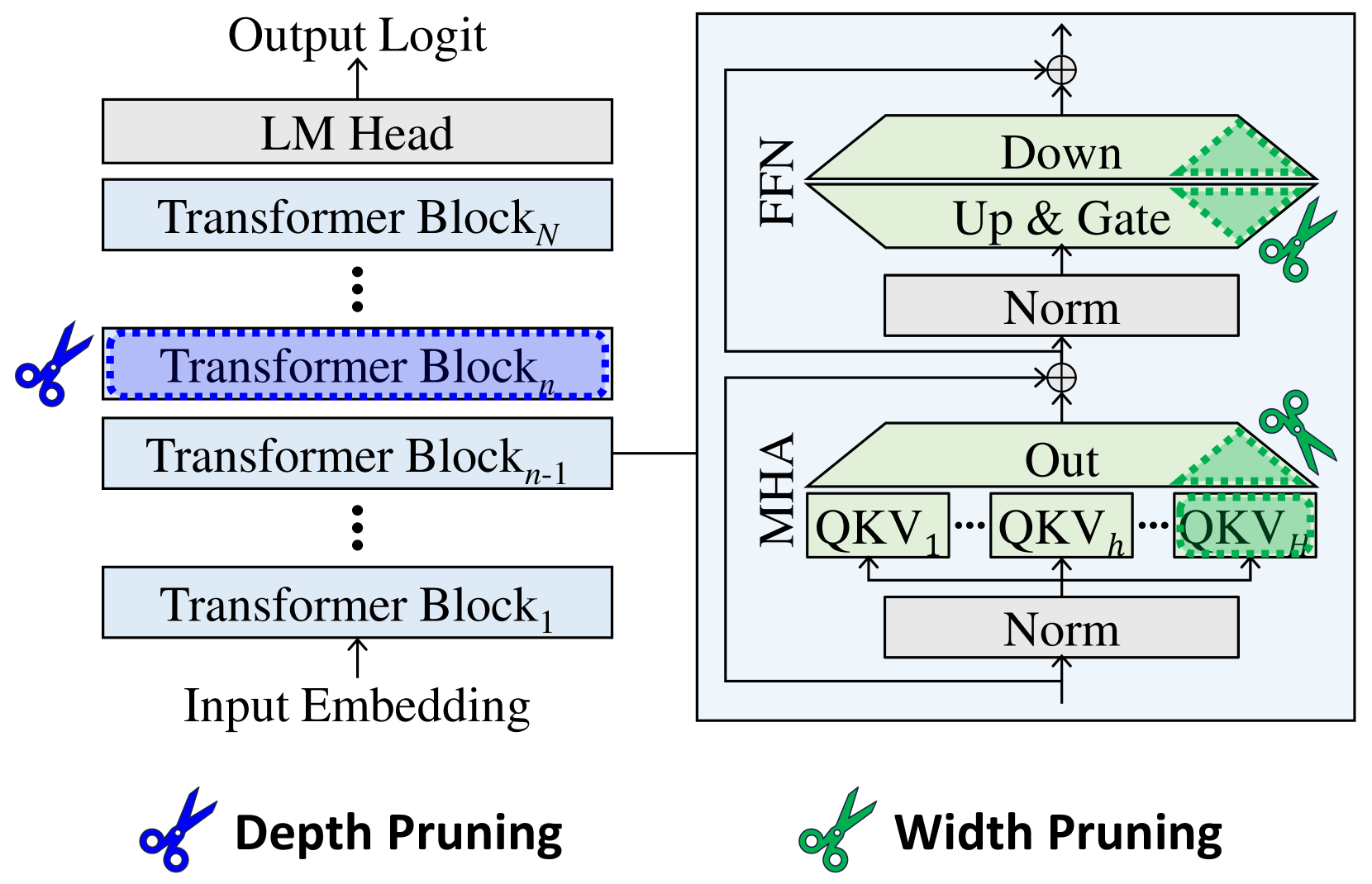</details> Figure 3: Comparison of pruning units. Width pruning reduces the size of projection weight matrices. Depth pruning removes Transformer blocks, or individual MHA and FFN modules. ## 2 Problem: Small-batch LLM Inference Most LLMs are autoregressive models that sequentially produce tokens, based on the initial prompt and the sequence of tokens previously generated. The token-by-token generation process often involves multiplying large matrices (weights) with smaller matrices or vectors (activations). The primary bottleneck for inference efficiency is memory access operations rather than the speed of mathematical computations (referred to as ‘memory-bound’), leading to suboptimal use of GPU computing power Kwon et al. (2023). Though increasing batch sizes is a standard way to enhance GPU computation and throughput, it poses a risk of out-of-memory (OOM) errors (see Figure 2) Using the HF-Transformers library Wolf et al. (2020), we ran the LLMs with 12 input tokens for 20 batched runs after 10 warm-ups. Top: Peak GPU compute utilization NVIDIA (2018). Bottom: Mean latency over 20 runs. unless advanced system-level optimizations Kwon et al. (2023); Sheng et al. (2023) are applied. In this study, our focus is on accelerating the inference of LLMs under small-batch conditions caused by hardware restrictions. Such situations are relevant for deploying LLMs on memory-constrained local devices, which can enhance user experience and data privacy protection. We show that (i) reducing weight shapes via width pruning does not improve generation speeds and can even degrade it when the resulting weight dimensions are unsuitable for GPU capabilities, and (ii) notable speed gains are only achievable through depth pruning that excludes a number of modules entirely. ## 3 Method: Block Pruning An LLM is a stack of multiple Transformer blocks Vaswani et al. (2017), each of which contains a pair of multi-head attention (MHA) and feed-forward network (FFN) modules (see Figure 3). We choose this Transformer block as the prunable unit to prioritize reducing inference latency. Our approach is simple: after identifying unimportant blocks with straightforward metrics, we perform simple one-shot pruning. ### 3.1 Evaluation of Block-level Importance We consider the following criteria to evaluate the significance of each block, ultimately selecting the Taylor+ and PPL metrics (see Table 6). Specifically, the linear weight matrix is denoted as $W^k,n=≤ft[W_i,j^k,n\right]$ with a size of $(d_out,d_in)$ , where $k$ represents the type of operation (e.g., a query projection in MHA or an up projection in FFN) within the $n$ -th Transformer block. The weight importance scores are calculated at the output neuron level Sun et al. (2024), followed by summing In our exploration of various aggregation strategies (i.e., sum, mean, product, and max operations), summing the scores was effective at different pruning ratios. these scores to assess the block-level importance. Magnitude (Mag). This metric Li et al. (2017b) is a fundamental baseline in the pruning literature, assuming that weights with smaller norms are less informative. For the block-level analysis, we compute $I_Magnitude^n=∑_k∑_i∑_j≤ft|W_i,j^k,n\right|$ . <details> <summary>x4.png Details</summary>  ### Visual Description ## [Chart Type]: Two-Panel Line Chart (Perplexity vs. Removed Block Index) ### Overview The image displays two vertically stacked plots analyzing the Perplexity (PPL) of two language models (LLaMA-7B and Vicuna-7B) as a function of the "Removed Block Index" (x-axis, 1–31). The top plot uses a **logarithmic y-axis** (PPL: \(10^2\) to \(10^4\)), while the bottom plot uses a **linear y-axis** (PPL: 20–35). Four data series are plotted: - LLaMA-7B: Single Block (orange crosses) - LLaMA-7B: Original (orange dashed line) - Vicuna-7B: Single Block (blue diamonds) - Vicuna-7B: Original (blue dashed line) ### Components/Axes - **X-axis (both plots)**: "Removed Block Index" with ticks at 1, 4, 7, 10, 13, 16, 19, 22, 25, 28, 31. - **Y-axis (top plot)**: "PPL" (logarithmic scale: \(10^2\), \(10^3\), \(10^4\)). - **Y-axis (bottom plot)**: "PPL" (linear scale: 20, 25, 30, 35). - **Legend (both plots)**: - Orange cross: LLaMA-7B: Single Block - Orange dashed line: LLaMA-7B: Original - Blue diamond: Vicuna-7B: Single Block - Blue dashed line: Vicuna-7B: Original ### Detailed Analysis (Top Plot: Logarithmic PPL) - **LLaMA-7B: Single Block (orange crosses)**: - Index 1: PPL ≈ \(10^4\) (10,000, extremely high). - Index 4: Drops sharply to ≈ \(10^2\) (100). - Indices 4–30: Remains stable at ≈ \(10^2\) (100). - Index 31: Slight rise to ≈ \(10^{2.1}\) (≈126). - **Vicuna-7B: Single Block (blue diamonds)**: - Index 1: PPL ≈ \(10^4\) (10,000, same as LLaMA-7B). - Index 4: Drops to ≈ \(10^2\) (100). - Indices 4–30: Remains stable at ≈ \(10^2\) (100). - Index 31: Slight rise to ≈ \(10^{2.1}\) (≈126). - **LLaMA-7B: Original (orange dashed line)**: Horizontal line at ≈ \(10^2\) (100, constant PPL). - **Vicuna-7B: Original (blue dashed line)**: Horizontal line at ≈ \(10^2\) (100, constant PPL). ### Detailed Analysis (Bottom Plot: Linear PPL) - **LLaMA-7B: Single Block (orange crosses)**: - Index 1: PPL ≈ 30. - Index 4: Drops to ≈ 23. - Indices 4–30: Fluctuates slightly (≈22–23). - Index 31: Rises to ≈ 25. - **Vicuna-7B: Single Block (blue diamonds)**: - Index 1: PPL ≈ 30 (same as LLaMA-7B). - Index 4: PPL ≈ 30 (no drop, unlike LLaMA-7B). - Indices 4–30: Fluctuates (≈27–30, with peaks at indices 19, 25). - Index 31: Rises to ≈ 30. - **LLaMA-7B: Original (orange dashed line)**: Horizontal line at ≈ 20 (constant PPL). - **Vicuna-7B: Original (blue dashed line)**: Horizontal line at ≈ 27 (constant PPL). ### Key Observations 1. **Initial Spike (Index 1)**: Both models have extremely high PPL when the first block is removed, indicating the first block is critical for performance. 2. **Drop at Index 4**: LLaMA-7B’s PPL drops sharply at index 4, while Vicuna-7B’s PPL remains high (≈30) until later indices. 3. **Stability (Indices 4–30)**: LLaMA-7B’s PPL stabilizes at a lower value (≈22–23) than Vicuna-7B (≈27–30) in the linear plot. 4. **Final Rise (Index 31)**: Both models show a PPL increase at index 31, suggesting the last block is also important (though less so than the first). 5. **Original Models**: LLaMA-7B Original has lower PPL (≈20) than Vicuna-7B Original (≈27), indicating LLaMA-7B performs better in its original form. ### Interpretation - **Block Importance**: The first block (index 1) is critical for both models (removing it causes a massive PPL spike). Blocks 2–3 are less critical (performance recovers after index 1). - **Model Comparison**: LLaMA-7B outperforms Vicuna-7B (lower PPL) when blocks are removed (except at index 1), suggesting LLaMA-7B is more robust to block removal. - **Original vs. Single Block**: Removing blocks generally degrades performance (single-block PPL > original PPL), but the degradation is less severe after the first block. - **Anomaly at Index 31**: The rise in PPL at index 31 implies the last block also contributes to performance, though its impact is smaller than the first block. This analysis reveals the critical role of the first block in model performance and highlights differences in robustness between LLaMA-7B and Vicuna-7B. 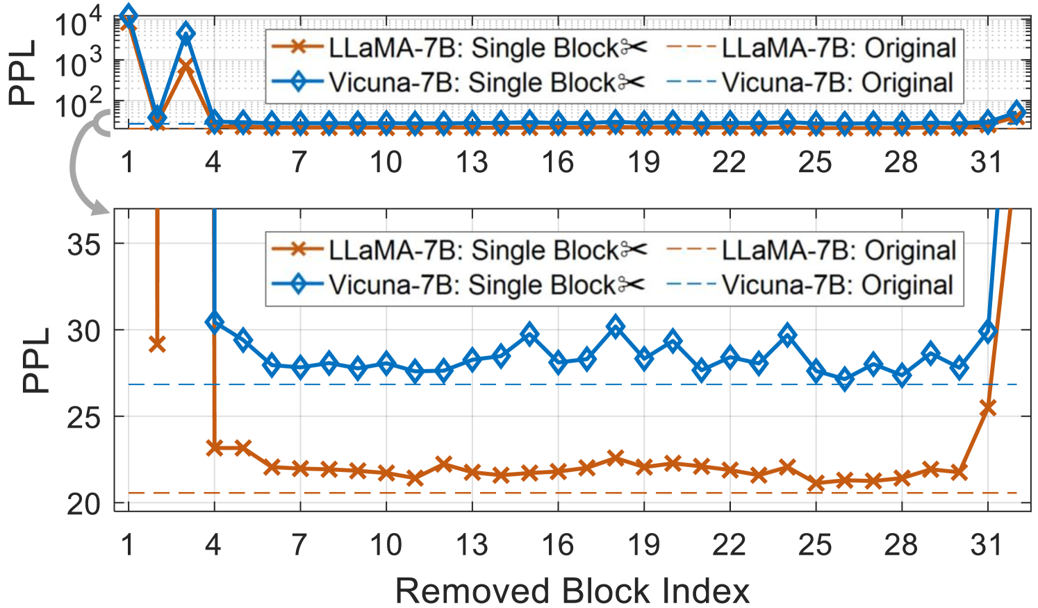</details> Figure 4: Estimated importance of each Transformer block on the calibration set. We prune blocks that have lower (better) PPL scores, as their removal causes less disruption to the output. Taylor. Assessing the error caused by the removal of a weight parameter helps in identifying its significance. For a given calibration dataset $D$ , this can be expressed as the alteration in the training loss $L$ LeCun et al. (1989); Molchanov et al. (2019): $≤ft|L(W_i,j^k,n;D)-L(W_i,j^k,n=0;D)\right| ≈≤ft|\frac{∂L(D)}{∂ W_i,j^k,n}W_i,j^k,n \right|$ , where we omit the second-order derivatives by following Ma et al. (2023). We define the block score as $I_Taylor^n=∑_k∑_i∑_j≤ft|\frac{∂L (D)}{∂ W_i,j^k,n}W_i,j^k,n\right|$ . Mag+ and Taylor+. Upon using the aforementioned metrics, the early blocks are labeled as unimportant, but their removal leads to severe performance drops. Similar to a popular heuristic Gale et al. (2019); Lee et al. (2021), we preserve the first four and the last two blocks Ma et al. (2023) by excluding them from the pruning candidates. Perplexity (PPL). Redundant blocks contribute less to the model’s outputs, and their removal leads to smaller degradation in PPL, a commonly used metric for language modeling tasks. In this context, we eliminate each block from the source model and monitor its influence on PPL using the calibration set $D$ : $I_PPL^n=\exp≤ft\{-\frac{1}{SL}∑_s∑_l\log p_θ^n (x_l^(s)|x_<l^(s))\right\}$ , where $θ^n$ denotes the model without its $n$ -th block, and $s=1,…,S$ and $l=1,…,L$ are the indices for sequences and tokens in $D$ . The PPL can be derived from the next-token prediction loss and requires only forward-pass computation. As shown in Figure 4, several blocks are removable with only a slight effect on the PPL metric. Pruning initial and final blocks significantly degrades the performance, which necessitates keeping them unpruned. ### 3.2 One-shot Pruning After sorting the block-level importance scores, we prune the less crucial blocks in a single step. Since every block has an identical configuration and it is easy to calculate the number of parameters for one block, we readily decide how many blocks should be removed to meet the target model size. Iterative pruning with intermediate updates of block importance can be applied as in SLEB Song et al. (2024). However, it requires much longer computing time than one-shot pruning as the number of blocks increases. Furthermore, we empirically observed that retraining strategies matter more than whether the pruning scheme is iterative or one-shot, especially under severe pruning ratios. ### 3.3 Retraining for Performance Restoration Some recent studies suggest that structured pruning of LLMs can be retraining-free Song et al. (2024); An et al. (2024) or feasible with low retraining budgets Ma et al. (2023). However, the types of retraining over different pruning rates have been underexplored. Here, we compare several retraining strategies and their implications for regaining the quality of pruned models. Low-Rank Adaptation (LoRA). LoRA Hu et al. (2022) enables the efficient refinement of LLMs with less computation. Ma et al. (2023) has applied LoRA to enhance moderately width-pruned models (e.g., with 20% of units removed) on an instruction tuning dataset. In this work, we show that LoRA can also recover the ability of depth-pruned models; however, it does not perform well for extensive compression rates (e.g., with over 50% removal) in either width or depth pruning. Continued Pretraining (CPT). We leverage CPT, which involves updating all parameters, on a large-scale pretraining corpus. This powerful retraining is critical for severely depth-pruned models, extending its proven effectiveness for width- or hybrid-pruned models Xia et al. (2024). Though requiring greater resources than LoRA, CPT on pruned networks significantly accelerates learning and yields superior results compared to training the same architectures from random initialization. CPT $⇒$ LoRA Once CPT on the pretraining data is completed, LoRA with the instruction set is applied to observe whether further performance improvement can be achieved. Model #Param #Block $‡$ #Head $‡$ FFN-D $‡$ Original 7B 6.7B 32 32 11008 35% $†$ Wanda-sp 4.5B 32 21 7156 FLAP 4.5B 32 23.0±8.8 6781.1±2440.6 LLM-Pruner 4.4B 32 18 6054 Ours 4.5B 21 32 11008 Original 13B 13.0B 40 40 13824 37% $†$ Wanda-sp 8.4B 40 26 8710 FLAP 8.3B 40 27.5±11.3 8326.6±2874.9 LLM-Pruner 8.2B 40 22 7603 Ours 8.3B 25 40 13824 $†$ Reduction ratio for the number of parameters. $‡$ #Block: #Transformer blocks; #Head: #attention heads of MHA; FFN-D: intermediate size of FFN. Table 1: Examples of pruned architectures on 7B-parameter (top) and 13B-parameter (bottom) models. While Wanda-sp Sun et al. (2024); An et al. (2024), FLAP An et al. (2024), and LLM-Pruner Ma et al. (2023) reduce the network width, our method reduces the network depth. See Table 14 for the details. Zero-shot Performance H100 80GB $‡$ RTX3090 24GB $‡$ PPL↓ #Param & Method WikiText2 PTB Ave Acc↑ (%) $†$ Latency↓ (s) Throughput↑ (tokens/s) Latency↓ (s) Throughput↑ (tokens/s) LLaMA-7B: 6.7B (Original) 12.6 22.1 66.3 2.4 53.7 5.1 25.0 Wanda-sp 21.4 47.2 51.8 3.1 41.7 7.6 16.7 FLAP 17.0 30.1 59.5 3.2 40.5 7.7 16.5 W✂ LLM-Pruner 17.6 30.4 61.8 3.0 43.2 6.0 21.4 SLEB 18.5 31.6 57.6 1.9 66.0 4.5 28.4 Ours: Taylor+ 20.2 32.3 63.5 1.9 66.0 4.5 28.4 5.5B (20% Pruned) D✂ Ours: PPL 17.7 30.7 61.9 1.9 66.0 4.5 28.4 Wanda-sp 133.6 210.1 36.9 3.1 41.6 8.0 16.1 FLAP 25.6 44.4 52.7 3.2 40.5 8.1 15.8 W✂ LLM-Pruner 24.2 40.7 55.5 2.9 44.4 6.1 21.1 SLEB 34.2 49.8 50.1 1.6 80.1 3.4 37.8 Ours: Taylor+ 33.2 58.5 55.4 1.6 80.1 3.4 37.8 4.5B (35% Pruned) D✂ Ours: PPL 23.1 38.8 55.2 1.6 80.1 3.4 37.8 Zero-shot Performance H100 80GB RTX3090 24GB PPL↓ #Param & Method WikiText2 PTB Ave Acc↑ (%) $†$ Latency↓ (s) Throughput↑ (tokens/s) Latency↓ (s) Throughput↑ (tokens/s) Vicuna-13B: 13.0B (Original) 14.7 51.6 68.3 2.8 45.5 OOM OOM Wanda-sp 19.0 71.8 63.6 3.8 34.1 9.8 12.9 FLAP 18.8 65.3 63.3 3.9 32.6 10.2 12.6 W✂ LLM-Pruner 16.0 57.0 65.3 3.8 34.0 7.5 17.3 SLEB 20.5 68.7 60.4 2.3 55.7 5.4 23.9 Ours: Taylor+ 18.1 61.6 66.7 2.3 55.7 5.4 23.9 10.5B (21% Pruned) D✂ Ours: PPL 16.1 56.5 64.9 2.3 55.7 5.4 23.9 Wanda-sp 36.6 123.5 52.7 3.8 33.8 10.5 12.6 FLAP 28.7 96.2 58.3 3.9 32.9 9.7 13.2 W✂ LLM-Pruner 22.2 74.0 59.7 3.6 35.6 7.1 18.0 SLEB 41.6 116.5 49.4 1.8 69.7 4.0 31.7 Ours: Taylor+ 34.2 90.4 61.4 1.8 69.7 4.0 31.7 8.3B (37% Pruned) D✂ Ours: PPL 22.1 73.6 59.1 1.8 69.7 4.0 31.7 $†$ Average accuracy on seven commonsense reasoning tasks. $‡$ Measured with 12 input tokens, 128 output tokens, and a batch size of 1 on a single GPU. Table 2: Results with moderate-level pruning on LLaMA-7B (top) and Vicuna-13B-v1.3 (bottom). Our depth pruning (D✂) with LoRA retraining achieves similar performance to width pruning (W✂) methods Sun et al. (2024); An et al. (2024); Ma et al. (2023) and outperforms the recent SLEB Song et al. (2024), while effectively accelerating LLM inference. See Table 9 for detailed results. Metric PPL↓ on WikiText2 Ave Acc↑ (%) $†$ Throughput↑ (tokens/s) $‡$ #Param after Pruning $⋆$ 5.5B 3.7B 2.7B 1.5B 5.5B 3.7B 2.7B 1.5B 5.5B 3.7B 2.7B 1.5B Wanda-sp 24.4 364.5 1370.1 8969.3 58.5 36.7 37.0 35.6 41.7 40.5 40.7 43.5 FLAP 22.0 63.1 589.3 28727.9 61.4 47.3 36.7 34.5 40.5 41.2 41.2 42.3 W✂ LLM-Pruner 19.6 38.8 66.4 202.9 60.1 50.1 44.3 38.4 43.2 43.4 43.9 44.8 SLEB 25.1 110.4 731.5 18730.8 55.6 40.2 39.1 37.4 66.0 84.0 107.4 182.5 Ours, LoRA 18.8 37.0 68.9 1002.2 60.7 47.0 40.1 37.1 Ours, CPT 14.3 16.0 17.1 20.5 61.5 57.1 55.0 49.2 D✂ Ours, CPT $⇒$ LoRA 14.8 16.5 17.8 21.1 63.1 57.4 55.0 49.0 66.0 (1.2×) 84.0 (1.6×) 107.4 (2.0×) 182.5 (3.4×) Vicuna-7B: 6.7B (Original) 17.1 65.9 53.7 $⋆$ The pruning ratios of 20%, 45%, 60%, and 80% lead to 5.5B, 3.7B, 2.7B, and 1.5B parameters, respectively. The PPL criterion is used to obtain our models. $†$ Average accuracy on seven commonsense reasoning tasks. $‡$ Measured with 12 input tokens, 128 output tokens, and a batch size of 1 on an NVIDIA H100 GPU. Table 3: Effectiveness of CPT under high compression rates on Vicuna-7B-v1.3. CPT is essential to regain the performance of extensively pruned models (e.g., fewer than 3.7B parameters), whereas retraining-free An et al. (2024); Song et al. (2024) and LoRA-based Ma et al. (2023) approaches yield unsatisfactory results. Model Generated Text Vicuna-7B AI can create a logo in seconds! You choose the design elements you like best from pre-made templates, and then the AI generates a unique logo design just for you. This is a great way to get a professional-looking logo without hiring … Wanda-sp AI can create a logo in seconds now. Inso Ison Im Ison Im I I was able can do do do now do now do now Innowhere you you you you you you you you you you you you you you you you you you you you you you you you you you you … FLAP AI can create a logo in seconds The V Just ing A A A A A A A A A, A A A A A S Just a. : S . No An , A A the A The The… The The… A, A A A A. A A A This A The Just A A A A The A A The A A A. and The A All T A A.. A the … LLM-Pruner AI can create a logo in seconds: 10 seconds! I’ve created a logo in minutes using an AI. It has only one image in front for 8 minutes. 4 hours = 65.000 + 12 hours Words: English Speech: 100 words in 5 minutes 1. 60 hours 2. 492 … SLEB AI can create a logo in seconds while. :). I have put. I believe it . →.]. Here least →… </<erus known). See →www.giftoings . </<.next]; info. I’ve don-> .…erutex“ Here for. to “Itin.g for the next….. .0.>1260070uro.‘s- … Ours, CPT AI can create a logo in seconds. Even if you don’t have a designer who knows the best layouts to use or what colors work best together, AI is already hard at work creating the perfect combination to your artwork. AI is also capable of … Table 4: Generation examples from the original Vicuna-7B and the 60%-pruned models with 2.7B parameters. ## 4 Experimental Setup Source Model. Our testbed includes LLaMA-7B Touvron et al. (2023) and Vicuna-{7B, 13B}-v1.3 Chiang et al. (2023), which are famous LLMs. Baseline. LLM-Pruner Ma et al. (2023), FLAP An et al. (2024), and Wanda-sp (i.e., a structured variant An et al. (2024) of Wanda Sun et al. (2024)) serve as the baselines for width pruning. Table 1 shows the pruned architectures under similar numbers of parameters. We also examine SLEB Song et al. (2024), a retraining-free block pruning method for LLMs, which has been concurrently introduced with our study. Section E.1 describes the baselines in detail. Data. Following Ma et al. (2023), we randomly select 10 samples from BookCorpus Zhu et al. (2015) to compute block-level significance during the pruning stage. We also use this calibration dataset for the baseline methods to ensure a fair comparison. In LoRA retraining, 50K samples of the refined Alpaca Taori et al. (2023) are used for instruction tuning. In CPT retraining, we leverage SlimPajama Soboleva et al. (2023), which consists of 627B tokens for LLM pretraining. Evaluation. Following Touvron et al. (2023), we measure zero-shot accuracy on commonsense reasoning datasets (i.e., BoolQ Clark et al. (2019), PIQA Bisk et al. (2020), HellaSwag Zellers et al. (2019), WinoGrande Sakaguchi et al. (2019), ARC-easy Clark et al. (2018), ARC-challenge Clark et al. (2018), and OpenbookQA Mihaylov et al. (2018)) using the lm-evaluation-harness package EleutherAI (2023). We also report zero-shot PPL on WikiText2 Merity et al. (2017) and PTB Marcus et al. (1993). Latency and Throughput. We follow Sheng et al. (2023) to measure the metrics. Given a batch size $M$ and an output sequence length $L$ (excluding the input length), the latency $T$ represents the time required to handle the given prompts and produce $ML$ output tokens. The throughput is computed as $ML/T$ . We report the average results from 20 runs after the initial 10 warm-up batches. Implementation. We use the Hugging Face’s Transformers library Wolf et al. (2020). For pruning and LoRA retraining, an NVIDIA A100 GPU is employed. For CPT retraining, eight NVIDIA H100 GPUs are utilized, with a training duration of less than two weeks for each model size. For inference, we opt for the default setup of the Transformers library. See Section E.2 for the details. ## 5 Results ### 5.1 Moderate Pruning and LoRA Retraining Tables 2 and 9 show the zero-shot performance and inference efficiency of differently pruned models. Here, our models are obtained using a light LoRA retraining setup. The width pruning methods Ma et al. (2023); An et al. (2024); Sun et al. (2024) do not improve LLM inference efficiency. Under limited input (batch) scales, the processing speed largely hinges on the frequency of memory access operations. Addressing this issue by merely reducing matrix sizes is challenging, unless they are completely removed. The speed even worsens compared to the original model due to GPU-unfriendly operation dimensions (e.g., the hidden sizes of FFN are often not divisible by 8 (Table 14), which hinders the effective utilization of GPU Tensor Cores Andersch et al. (2019)). On the contrary, our depth pruning exhibits speedups through the complete removal of several Transformer blocks, resulting in fewer memory access and matrix-level operations between activations and weights. Moreover, under the same LoRA retraining protocol as Ma et al. (2023), our models achieve zero-shot scores on par with finely width-pruned models. Although SLEB Song et al. (2024) enhances inference efficiency similar to our method, its approach without retraining falls short in developing proficient small LLMs. See Section B for detailed results. <details> <summary>x5.png Details</summary>  ### Visual Description ## [Dual-Panel Line Chart]: Training Performance Comparison of Random vs. Pruned Initialization ### Overview The image displays two side-by-side line charts comparing the training performance of two model initialization methods: "Random Init." and "Pruned Init." over the course of training steps. The left chart tracks Perplexity (PPL), a measure of prediction error, while the right chart tracks Average Accuracy (Ave Acc) as a percentage. Both charts share the same X-axis (Update Steps) and legend. ### Components/Axes **Left Chart (PPL vs. Steps):** * **Y-axis:** Label: "PPL". Scale: Linear, ranging from approximately 17 to 41. Major tick marks at 17, 25, 33, 41. * **X-axis:** Label: "Update Steps". Scale: Linear, ranging from 0 to 120,000 (120K). Major tick marks at 0, 40K, 80K, 120K. * **Legend:** Positioned in the top-left quadrant of the chart area. Contains two entries: * "Random Init." - Represented by a light purple/lavender line. * "Pruned Init." - Represented by a solid blue line. **Right Chart (Ave Acc vs. Steps):** * **Y-axis:** Label: "Ave Acc (%)". Scale: Linear, ranging from approximately 35% to 56%. Major tick marks at 35, 42, 49, 56. * **X-axis:** Label: "Update Steps". Identical to the left chart (0 to 120K). * **Legend:** Positioned in the bottom-right quadrant of the chart area. Identical entries and color coding as the left chart. ### Detailed Analysis **Left Chart - Perplexity (PPL):** * **Trend Verification:** Both lines show a steep initial decrease followed by a gradual leveling off, indicating learning and convergence. The "Pruned Init." (blue) line decreases more rapidly and maintains a lower value throughout. * **Data Points (Approximate):** * **Random Init. (Light Purple):** Starts above 41 at step 0. Drops to ~25 by 20K steps, ~21 by 60K steps, and ends near ~19 at 120K steps. * **Pruned Init. (Blue):** Starts above 41 at step 0. Drops sharply to ~21 by 10K steps, ~19 by 40K steps, and ends near ~17 at 120K steps. **Right Chart - Average Accuracy (Ave Acc %):** * **Trend Verification:** Both lines show a steep initial increase followed by a gradual plateau, indicating improving model performance. The "Pruned Init." (blue) line increases more rapidly and maintains a higher accuracy throughout. * **Data Points (Approximate):** * **Random Init. (Light Purple):** Starts at ~35% at step 0. Rises to ~45% by 20K steps, ~50% by 60K steps, and ends near ~52% at 120K steps. * **Pruned Init. (Blue):** Starts at ~35% at step 0. Rises sharply to ~50% by 10K steps, ~53% by 40K steps, and ends near ~55% at 120K steps. ### Key Observations 1. **Consistent Superiority:** The "Pruned Init." method (blue line) demonstrates superior performance on both metrics (lower PPL, higher Accuracy) compared to "Random Init." (light purple line) at every comparable point after initialization. 2. **Faster Convergence:** The "Pruned Init." curves show a steeper initial slope in both charts, indicating it learns and converges to a good solution significantly faster in the early stages of training (first ~20K steps). 3. **Performance Gap:** A consistent performance gap is maintained between the two methods throughout the displayed training period (120K steps). The gap appears slightly larger in the Accuracy chart than in the PPL chart. 4. **Noise:** Both lines exhibit minor fluctuations (noise), which is typical for training curves, but the overall trends are clear and distinct. ### Interpretation The data strongly suggests that using a "Pruned Initialization" method provides a substantial advantage over standard random initialization for this specific model training task. The benefits are twofold: 1. **Improved Final Performance:** The model achieves a better final state, characterized by lower perplexity (better predictive likelihood) and higher average accuracy. 2. **Training Efficiency:** The model reaches a given performance level (e.g., 50% accuracy or PPL of 21) in far fewer update steps, which translates to reduced computational cost and training time. The relationship between the two charts is complementary: the decrease in PPL (error) directly correlates with the increase in Accuracy (correctness). The "Pruned Init." method's ability to drive both metrics more effectively from the start implies that the pruning process likely identifies and preserves a more optimal subnetwork or parameter structure within the model, providing a better starting point for the optimization process. This is a clear demonstration of the value of intelligent initialization strategies in machine learning. 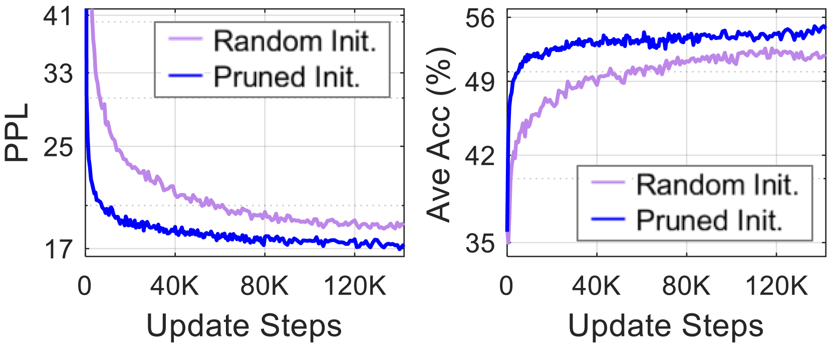</details> Figure 5: Zero-shot scores during the training progress of the 2.7B-parameter model from Vicuna-7B. Using the pruned network as initialization (blue lines) for CPT accelerates the learning process and yields better results than starting from scratch (purple). ### 5.2 Aggressive Pruning and CPT Retraining Table 3 compares different retraining methods. Our models are obtained using the PPL criterion. Under high pruning ratios (e.g., yielding fewer than 3.7B parameters), LoRA-based tuning (LLM-Pruner Ma et al. (2023); Ours, LoRA) and retraining-free approaches (Wanda-sp Sun et al. (2024); An et al. (2024), FLAP An et al. (2024), SLEB Song et al. (2024)) fail to recover model performance. In contrast, CPT proves effective in regaining the quality of heavily pruned models. CPT $⇒$ LoRA slightly improves zero-shot accuracy for some pruning ratios, but with a minor drop in PPL. Table 4 presents samples produced by 2.7B-parameter models (60% pruned). In contrast to the baselines, our model can generate text that is fluent and appropriately aligned with the context. Compared to LoRA retraining, the computational costs for CPT are considerably higher: LoRA can be completed within a day using just one GPU, while CPT requires about two weeks with eight GPUs in our experiments, with the option to use more if needed. However, utilizing a pruned network for initialization in CPT leads to faster learning and better results than building the same-sized models from scratch (see Figure 5), highlighting its efficacy for smaller LLMs. Section C presents the learning progress in detail. <details> <summary>extracted/5685909/fig/gptq_results.png Details</summary>  ### Visual Description ## [Bar Charts]: VRAM Usage and Average Accuracy vs. Model Parameter Count ### Overview The image displays two side-by-side bar charts comparing the performance of different model variants across four model sizes (2.7B, 3.7B, 5.5B, and 6.7B parameters). The left chart measures Video RAM (VRAM) usage in Gigabytes (GB), and the right chart measures Average Accuracy (Ave Acc) as a percentage. The comparison involves four model configurations: "Ours," "Ours + GPTQ," "Original," and "Original + GPTQ." ### Components/Axes * **Legend (Top-Center, spanning both charts):** * **Blue Bar:** "Ours" * **Teal Bar:** "Ours + GPTQ" * **Black Bar:** "Original" * **Gray Bar:** "Original + GPTQ" * **Left Chart - VRAM (GB):** * **Y-axis:** Label: "VRAM (GB)". Scale: 2 to 12, with major ticks every 2 units. * **X-axis:** Label: "# Parameters". Categories: "2.7B", "3.7B", "5.5B", "6.7B". * **Right Chart - Ave Acc (%):** * **Y-axis:** Label: "Ave Acc (%)". Scale: 52.5 to 65.0, with major ticks every 2.5 units. * **X-axis:** Label: "# Parameters". Categories: "2.7B", "3.7B", "5.5B", "6.7B". ### Detailed Analysis **Left Chart: VRAM (GB)** * **Trend Verification:** For the "Ours" (blue) and "Ours + GPTQ" (teal) series, VRAM usage increases with the number of parameters. The "Original" (black) and "Original + GPTQ" (gray) series are only present for the 6.7B parameter model. * **Data Points (Approximate Values):** * **2.7B Parameters:** * Ours (Blue): ~5.2 GB * Ours + GPTQ (Teal): ~2.6 GB * **3.7B Parameters:** * Ours (Blue): ~7.1 GB * Ours + GPTQ (Teal): ~3.1 GB * **5.5B Parameters:** * Ours (Blue): ~10.5 GB * Ours + GPTQ (Teal): ~4.1 GB * **6.7B Parameters:** * Original (Black): ~12.4 GB * Original + GPTQ (Gray): ~4.8 GB **Right Chart: Ave Acc (%)** * **Trend Verification:** For all series, average accuracy generally increases with the number of parameters. The "Ours" and "Ours + GPTQ" bars are very close in height for each parameter size, indicating minimal accuracy difference. * **Data Points (Approximate Values):** * **2.7B Parameters:** * Ours (Blue): ~55.0% * Ours + GPTQ (Teal): ~54.6% * **3.7B Parameters:** * Ours (Blue): ~57.2% * Ours + GPTQ (Teal): ~57.2% * **5.5B Parameters:** * Ours (Blue): ~61.5% * Ours + GPTQ (Teal): ~60.7% * **6.7B Parameters:** * Original (Black): ~66.0% * Original + GPTQ (Gray): ~63.5% ### Key Observations 1. **VRAM Reduction with GPTQ:** Applying GPTQ quantization ("Ours + GPTQ" vs. "Ours", and "Original + GPTQ" vs. "Original") results in a dramatic reduction in VRAM usage across all model sizes. The reduction is most pronounced for the 6.7B model, where VRAM drops from ~12.4 GB to ~4.8 GB. 2. **Accuracy Impact of GPTQ:** The impact of GPTQ on average accuracy is minimal for the "Ours" models (a difference of less than ~1% for 2.7B and 5.5B, and no difference for 3.7B). For the 6.7B "Original" model, GPTQ causes a more noticeable accuracy drop of approximately 2.5 percentage points. 3. **Model Comparison at 6.7B:** At the largest parameter size (6.7B), the "Original" model achieves the highest accuracy (~66.0%) but also requires the most VRAM (~12.4 GB). The "Original + GPTQ" variant offers a significant memory saving (~4.8 GB) with a moderate accuracy trade-off (~63.5%). 4. **Scaling Trend:** Both VRAM usage and average accuracy scale positively with the number of parameters for all model configurations. ### Interpretation This data demonstrates the trade-offs between model size, memory efficiency, and performance. The primary finding is the effectiveness of GPTQ quantization in drastically reducing VRAM requirements (by more than 50% in most cases) with a relatively small cost to accuracy, especially for the "Ours" model architecture. This suggests that the "Ours" method may be more robust to quantization than the "Original" method at the 6.7B scale. The charts are likely from a research paper or technical report aiming to showcase a new model architecture ("Ours") and its compatibility with post-training quantization techniques like GPTQ. The key message is that one can deploy larger, more accurate models (like the 6.7B variant) within practical memory constraints by applying GPTQ, making advanced AI models more accessible for deployment on consumer or edge hardware. The absence of "Original" data for smaller models implies the study's focus is on comparing the two architectures at the largest scale or that "Ours" is a new method being proposed for these model sizes. 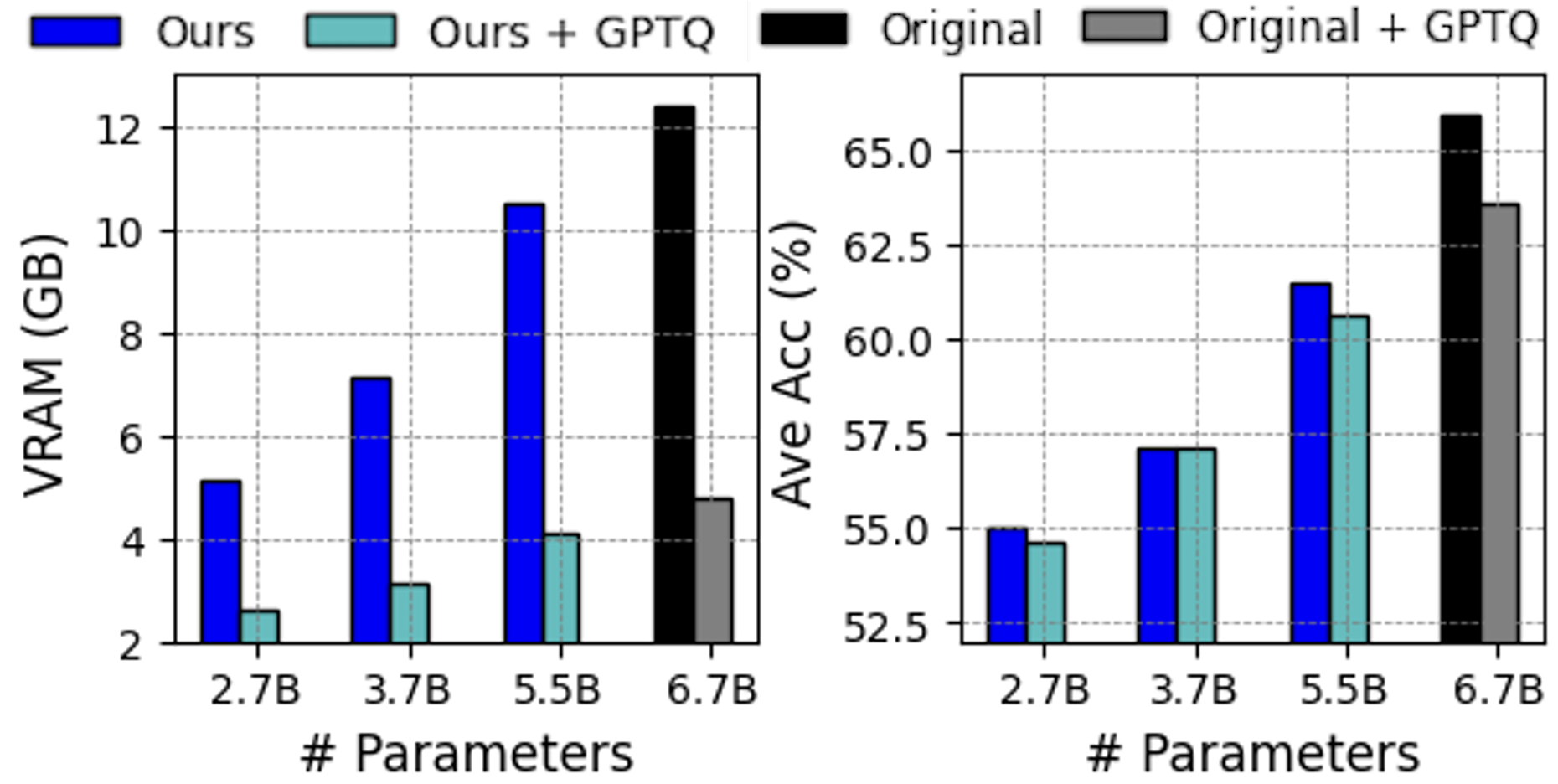</details> Figure 6: Further compression with GPTQ. Our pruned models following 4-bit weight quantization exhibit reduced VRAM usage without significant performance decline. The results for the original Vicuna-7B are presented for reference. See Section D for the details. ### 5.3 Applicability with Quantization Leveraging post-training quantization (PTQ) effectively lowers the memory consumption for inference of LLMs. Figure 6 shows the results of applying GPTQ Frantar et al. (2023), a well-known PTQ method, to our depth-pruned models after CPT. The 4-bit weight quantization significantly reduces the VRAM demands across various model sizes without noticeable degradation in zero-shot accuracy. See Section D for further results. ### 5.4 Ablation Study We explore various design factors, including the criteria for importance evaluation, the choice of units for depth pruning, and the impact of calibration data volume. The results presented in this section were obtained through LoRA retraining. #### 5.4.1 Importance Criteria for Block Pruning Table 6 presents the results of block pruning using various significance criteria. The basic methods without the ‘+’ label fail to maintain essential initial blocks, causing a decline in performance. The Mag+ method, which preserves these critical blocks, partially improves the scores; however, its effectiveness is still inferior compared to the other methods, indicating that relying solely on weight magnitude could be improper for pruning decisions. The Taylor+ criterion enhances accuracy in commonsense reasoning tasks, while the PPL method leads to better generation quality without relying on heuristic selection of pruning candidates. #### 5.4.2 Structural Unit for Depth Pruning Pruning individual MHA and FFN modules, which are more fine-grained units than Transformer blocks, is also possible. To examine its effect, we measure the impact of removing each module on the PPL of the calibration set and selectively eliminate the unnecessary modules. The same LoRA retraining procedure is conducted. Block Pruning Criterion PPL↓ Ave Acc↑ (%) $†$ WikiText2 PTB 5.5B (20% Pruned) Mag 7720.7 10618.7 34.4 Mag+ 19.4 36.3 56.1 Taylor 3631.7 4327.9 35.5 Taylor+ 20.2 32.3 63.5 PPL 17.7 30.7 61.9 4.5B (35% Pruned) Mag 8490.1 14472.1 34.9 Mag+ 36.9 61.1 49.3 Taylor 7666.8 10913.1 35.3 Taylor+ 33.2 58.5 55.4 PPL 23.1 38.8 55.2 $†$ Average accuracy on seven commonsense reasoning tasks. Table 5: Comparison of pruning criteria on LLaMA-7B. The Taylor+ method excels in commonsense reasoning accuracy, while the PPL criterion leads to better generation performance. Depth Pruning Unit #Param PPL↓ Ave Acc↑ (%) $†$ WikiText2 PTB Individual MHA & FFN 5.7B 20.8 34.8 63.1 Transformer Block 5.7B 16.9 29.3 62.8 Individual MHA & FFN 5.3B 25.2 41.3 61.1 Transformer Block 5.3B 18.6 33.1 60.6 Individual MHA & FFN 4.6B 38.9 58.7 52.5 Transformer Block 4.5B 23.1 38.8 55.2 Individual MHA & FFN 4.0B 63.2 88.9 48.3 Transformer Block 3.9B 31.1 47.3 50.6 $†$ Average accuracy on seven commonsense reasoning tasks. Table 6: Comparison of depth pruning granularities on LLaMA-7B. Removing entire Transformer blocks instead of individual MHA and FFN modules generally yields better results. Table 6 shows the results of depth pruning at different granularities. For the models with more than 5B parameters, removing individual MHA and FFN modules results in better downstream task accuracy but worse PPL compared to removing entire Transformer blocks. For smaller models than 5B, block-level pruning achieves superior results in terms of all the examined metrics. This differs from the common belief that removing finer units yields better performance. Given the collaborative roles of the modules (i.e., MHA captures dependency relations Vaswani et al. (2017), while skip connections and FFN prevent the rank collapse in purely attention-driven networks Dong et al. (2021)), it may be suboptimal to treat them in isolation. Taking the 5.3B model in Table 6 as an example, module-level pruning results in consecutive FFNs in some positions, potentially impairing the model’s ability to handle word interactions. In contrast, with block-level removal, the loss of information could be compensated by neighboring blocks that serve similar functions. #### 5.4.3 Calibration Data Volume The calibration set is employed to assess the weight significance of width pruning baselines and the block-level importance of our method during the pruning phase. Table 7 presents the results obtained by varying the number of calibration samples in the BookCorpus dataset. The scores remain relatively stable for the examined methods, suggesting that 10 samples could be sufficient. However, our Taylor+ method encounters a drop in downstream task accuracy when 1K samples are used, leaving the exploration of calibration data characteristics for future research. ## 6 Related Work Numerous techniques have been developed towards efficient LLMs, including knowledge distillation Fu et al. (2023); Hsieh et al. (2023), quantization Frantar et al. (2023); Dettmers et al. (2022), and system-level inference acceleration Dao (2023); Kwon et al. (2023). In this study, we focus on network pruning LeCun et al. (1989), which has a long-standing reputation in the model compression field. Beyond its use in relatively small-scale convolutional networks Li et al. (2017b); He et al. (2019) and Transformer models Yu et al. (2022); Xia et al. (2022); Kurtic et al. (2023), pruning has recently begun to be applied to contemporary LLMs. Several studies Frantar and Alistarh (2023); Sun et al. (2024) employ unstructured and semi-structured Aojun Zhou (2021) pruning by zeroing individual neurons. SparseGPT Frantar and Alistarh (2023) addresses the layer-wise reconstruction problem for pruning by computing Hessian inverses. Wanda Sun et al. (2024) introduces a pruning criterion that involves multiplying weight magnitudes by input feature norms. Despite the plausible performance of pruned models using zero masks, they necessitate specialized support for sparse matrix operations to ensure actual speedups. In contrast, structured pruning removes organized patterns, such as layers Fan et al. (2020); Jha et al. (2023), MHA’s attention heads Voita et al. (2019); Michel et al. (2022), FFN’s hidden sizes Nova et al. (2023); Santacroce et al. (2023), and some hybrid forms Lagunas et al. (2021); Xia et al. (2022); Kwon et al. (2022); Kurtic et al. (2023), thereby improving inference efficiency in a hardware-agnostic way. To compress LLMs, FLAP An et al. (2024) and LLM-Pruner Ma et al. (2023) eliminate coupled structures in the aspect of network width while retaining the number of layers. Sheared-LLaMA Xia et al. (2024) introduces a mask learning phase aimed at identifying prunable components in both the network’s width and depth. Our study explores the relatively untapped area of depth-only pruning for multi-billion parameter LLMs, which can markedly accelerate latency while attaining competitive performance. Strategies for skipping layers Schuster et al. (2022); Corro et al. (2023); Raposo et al. (2024) effectively serve to decrease computational burdens. Moreover, depth pruning approaches Song et al. (2024); Men et al. (2024); Tang et al. (2024) for LLMs have been proposed concurrently with our work, based on the architectural redundancy in LLMs. Evaluation Metric Method # Calibration Samples 10 50 100 1000 PPL↓ on WikiText2 Wanda-sp 21.4 21.4 21.7 20.8 FLAP 17.0 17.5 17.5 17.3 LLM-Pruner 17.6 17.2 17.0 OOM $‡$ Ours: Taylor+ 20.2 20.2 19.0 19.6 Ours: PPL 17.7 17.2 17.4 17.4 Ave Acc↑ (%) $†$ Wanda-sp 51.8 52.9 52.0 53.0 FLAP 59.5 59.7 59.9 60.8 LLM-Pruner 61.8 61.6 61.7 OOM $‡$ Ours: Taylor+ 63.5 63.5 63.9 61.7 Ours: PPL 61.9 61.5 61.7 61.7 $†$ Average accuracy on seven commonsense reasoning tasks. $‡$ Out-of-memory error on an A100 (80GB) using the official code. Table 7: Impact of calibration data volume. The results of 20%-pruned LLaMA-7B are reported. ## 7 Conclusion By introducing a block pruning method, we conduct an in-depth comparative analysis on the impact of network width and depth on LLM compression. Our work involves the one-shot removal of Transformer blocks. Despite its simplicity, our method with light LoRA retraining matches the zero-shot capabilities of recent width pruning techniques under moderate pruning levels. Moreover, it offers significant inference speedups in resource-constrained scenarios that require running LLMs with limited batch sizes, where width pruning falls short. When comparing retraining strategies, continued pretraining on a large-scale dataset significantly surpasses LoRA-based tuning, particularly in cases of severe pruning. We hope this study will support the development of potent small LLMs. ## Limitations Due to constraints in computational resources, we could not test our method on LLMs exceeding 13B parameters. We plan to explore larger models in future research, given that our method can be applied to any model size. Secondly, we found that continued pretraining was essential for performance recovery after extensive pruning. Further exploration of different training corpora and hyperparameters could lead to additional performance improvements. Lastly, commercially available LLMs are optimized for human preferences, such as safety and helpfulness, through alignment tuning. We have yet to assess human preferences throughout the entire process of pruning, retraining, and quantization. We hope future research will address this aspect. ## Acknowledgments We thank the Microsoft Startups Founders Hub program and the AI Industrial Convergence Cluster Development project funded by the Ministry of Science and ICT (MSIT, Korea) and Gwangju Metropolitan City for their generous support of GPU resources. ## References - An et al. (2024) Yongqi An, Xu Zhao, Tao Yu, Ming Tang, and Jinqiao Wang. 2024. Fluctuation-based adaptive structured pruning for large language models. In AAAI. - Andersch et al. (2019) Michael Andersch, Valerie Sarge, and Paulius Micikevicius. 2019. Tensor core dl performance guide. In NVIDIA GTC. - Aojun Zhou (2021) Junnan Zhu Jianbo Liu Zhijie Zhang Kun Yuan Wenxiu Sun Hongsheng Li Aojun Zhou, Yukun Ma. 2021. Learning n:m fine-grained structured sparse neural networks from scratch. In ICLR. - Bisk et al. (2020) Yonatan Bisk, Rowan Zellers, Ronan Le Bras, Jianfeng Gao, and Yejin Choi. 2020. Piqa: Reasoning about physical commonsense in natural language. In AAAI. - Chiang et al. (2023) Wei-Lin Chiang, Zhuohan Li, Zi Lin, Ying Sheng, Zhanghao Wu, Hao Zhang, Lianmin Zheng, et al. 2023. Vicuna: An open-source chatbot impressing gpt-4 with 90%* chatgpt quality. - Chowdhery et al. (2022) Aakanksha Chowdhery, Sharan Narang, Jacob Devlin, Maarten Bosma, Gaurav Mishra, Adam Roberts, Paul Barham, Hyung Won Chung, et al. 2022. Palm: Scaling language modeling with pathways. arXiv preprint arXiv:2204.02311. - Clark et al. (2019) Christopher Clark, Kenton Lee, Ming-Wei Chang, Tom Kwiatkowski, Michael Collins, and Kristina Toutanova. 2019. BoolQ: Exploring the surprising difficulty of natural yes/no questions. In NAACL. - Clark et al. (2018) Peter Clark, Isaac Cowhey, Oren Etzioni, Tushar Khot, Ashish Sabharwal, Carissa Schoenick, and Oyvind Tafjord. 2018. Think you have solved question answering? try arc, the ai2 reasoning challenge. arXiv preprint arXiv:1803.05457. - Corro et al. (2023) Luciano Del Corro, Allie Del Giorno, Sahaj Agarwal, Bin Yu, Ahmed Awadallah, and Subhabrata Mukherjee. 2023. Skipdecode: Autoregressive skip decoding with batching and caching for efficient llm inference. arXiv preprint arXiv:2307.02628. - Dao (2023) Tri Dao. 2023. Flashattention-2: Faster attention with better parallelism and work partitioning. arXiv preprint arXiv:2307.08691. - Dettmers et al. (2022) Tim Dettmers, Mike Lewis, Younes Belkada, and Luke Zettlemoyer. 2022. Llm.int8(): 8-bit matrix multiplication for transformers at scale. In NeurIPS. - Dong et al. (2021) Yihe Dong, Jean-Baptiste Cordonnier, and Andreas Loukas. 2021. Attention is not all you need: Pure attention loses rank doubly exponentially with depth. In ICML. - EleutherAI (2023) EleutherAI. 2023. Language model evaluation harness (package version 3326c54). https://github.com/EleutherAI/lm-evaluation-harness. - Fan et al. (2020) Angela Fan, Edouard Grave, and Armand Joulin. 2020. Reducing transformer depth on demand with structured dropout. In ICLR. - Fang et al. (2023) Gongfan Fang, Xinyin Ma, Mingli Song, Michael Bi Mi, and Xinchao Wang. 2023. Depgraph: Towards any structural pruning. In CVPR. - Frantar and Alistarh (2023) Elias Frantar and Dan Alistarh. 2023. SparseGPT: Massive language models can be accurately pruned in one-shot. In ICML. - Frantar et al. (2023) Elias Frantar, Saleh Ashkboos, Torsten Hoefler, and Dan Alistarh. 2023. OPTQ: Accurate quantization for generative pre-trained transformers. In ICLR. - Fu et al. (2023) Yao Fu, Hao Peng, Litu Ou, Ashish Sabharwal, and Tushar Khot. 2023. Specializing smaller language models towards multi-step reasoning. In ICML. - Gale et al. (2019) Trevor Gale, Erich Elsen, and Sara Hooker. 2019. The state of sparsity in deep neural networks. In ICML Workshop. - Google (2023) Google. 2023. An important next step on our ai journey. https://blog.google/technology/ai/bard-google-ai-search-updates/. - He et al. (2019) Yang He, Ping Liu, Ziwei Wang, Zhilan Hu, and Yi Yang. 2019. Filter pruning via geometric median for deep convolutional neural networks acceleration. In CVPR. - Hsieh et al. (2023) Cheng-Yu Hsieh, Chun-Liang Li, Chih-Kuan Yeh, Hootan Nakhost, et al. 2023. Distilling step-by-step! outperforming larger language models with less training data and smaller model sizes. In Findings of ACL. - Hu et al. (2022) Edward J. Hu, Yelong Shen, Phillip Wallis, Zeyuan Allen-Zhu, Yuanzhi Li, Shean Wang, Lu Wang, and Weizhu Chen. 2022. Lora: Low-rank adaptation of large language models. In ICLR. - Jha et al. (2023) Ananya Harsh Jha, Tom Sherborne, Evan Pete Walsh, Dirk Groeneveld, Emma Strubell, and Iz Beltagy. 2023. How to train your (compressed) large language model. arXiv preprint arXiv:2305.14864. - Jin et al. (2023) Yunho Jin, Chun-Feng Wu, David Brooks, and Gu-Yeon Wei. 2023. S3: Increasing gpu utilization during generative inference for higher throughput. In NeurIPS. - Kurtic et al. (2023) Eldar Kurtic, Elias Frantar, and Dan Alistarh. 2023. Ziplm: Inference-aware structured pruning of language models. In NeurIPS. - Kwon et al. (2022) Woosuk Kwon, Sehoon Kim, Michael W. Mahoney, Joseph Hassoun, Kurt Keutzer, and Amir Gholami. 2022. A fast post-training pruning framework for transformers. In NeurIPS. - Kwon et al. (2023) Woosuk Kwon, Zhuohan Li, Siyuan Zhuang, Ying Sheng, Lianmin Zheng, Cody Hao Yu, Joseph E. Gonzalez, Hao Zhang, and Ion Stoica. 2023. Efficient memory management for large language model serving with pagedattention. In SOSP. - Lagunas et al. (2021) François Lagunas, Ella Charlaix, Victor Sanh, and Alexander M. Rush. 2021. Block pruning for faster transformers. In EMNLP. - LeCun et al. (1989) Yann LeCun, John Denker, and Sara Solla. 1989. Optimal brain damage. In NeurIPS. - Lee et al. (2021) Jaeho Lee, Sejun Park, Sangwoo Mo, Sungsoo Ahn, and Jinwoo Shin. 2021. Layer-adaptive sparsity for the magnitude-based pruning. In ICLR. - Li et al. (2017a) Hao Li, Asim Kadav, Igor Durdanovic, Hanan Samet, and Hans Peter Graf. 2017a. Pruning filters for efficient convnets. In ICLR. - Li et al. (2017b) Hao Li, Asim Kadav, Igor Durdanovic, Hanan Samet, and Hans Peter Graf. 2017b. Pruning filters for efficient convnets. In ICLR. - Ma et al. (2023) Xinyin Ma, Gongfan Fang, and Xinchao Wang. 2023. Llm-pruner: On the structural pruning of large language models. In NeurIPS. - Marcus et al. (1993) Mitchell P. Marcus, Beatrice Santorini, and Mary Ann Marcinkiewicz. 1993. Building a large annotated corpus of English: The Penn Treebank. Computational Linguistics, 19(2):313–330. - Men et al. (2024) Xin Men, Mingyu Xu, Qingyu Zhang, Bingning Wang, Hongyu Lin, Yaojie Lu, Xianpei Han, and Weipeng Chen. 2024. Shortgpt: Layers in large language models are more redundant than you expect. arXiv preprint arXiv:2403.03853. - Merity et al. (2017) Stephen Merity, Caiming Xiong, James Bradbury, and Richard Socher. 2017. Pointer sentinel mixture models. In ICLR. - Michel et al. (2022) Paul Michel, Omer Levy, and Graham Neubig. 2022. Are sixteen heads really better than one? In NeurIPS. - Mihaylov et al. (2018) Todor Mihaylov, Peter Clark, Tushar Khot, and Ashish Sabharwal. 2018. Can a suit of armor conduct electricity? a new dataset for open book question answering. In EMNLP. - Molchanov et al. (2019) Pavlo Molchanov, Arun Mallya, Stephen Tyree, Iuri Frosio, and Jan Kautz. 2019. Importance estimation for neural network pruning. In CVPR. - Nova et al. (2023) Azade Nova, Hanjun Dai, and Dale Schuurmans. 2023. Gradient-free structured pruning with unlabeled data. In ICML. - NVIDIA (2018) NVIDIA. 2018. Useful nvidia-smi queries. https://enterprise-support.nvidia.com/s/article/Useful-nvidia-smi-Queries-2. - OpenAI (2022) OpenAI. 2022. Introducing chatgpt. https://openai.com/blog/chatgpt. - OpenAI (2023) OpenAI. 2023. Gpt-4 technical report. arXiv preprint arXiv:2303.08774. - Raffel et al. (2020) Colin Raffel, Noam Shazeer, Adam Roberts, Katherine Lee, Sharan Narang, Michael Matena, Yanqi Zhou, Wei Li, and Peter J Liu. 2020. Exploring the limits of transfer learning with a unified text-to-text transformer. JMLR, 21(140):1–67. - Raposo et al. (2024) David Raposo, Sam Ritter, Blake Richards, Timothy Lillicrap, Peter Conway Humphreys, and Adam Santoro. 2024. Mixture-of-depths: Dynamically allocating compute in transformer-based language models. arXiv preprint arXiv:2404.02258. - Sakaguchi et al. (2019) Keisuke Sakaguchi, Ronan Le Bras, Chandra Bhagavatula, and Yejin Choi. 2019. Winogrande: An adversarial winograd schema challenge at scale. arXiv preprint arXiv:1907.10641. - Santacroce et al. (2023) Michael Santacroce, Zixin Wen, Yelong Shen, and Yuanzhi Li. 2023. What matters in the structured pruning of generative language models? arXiv preprint arXiv:2302.03773. - Scao et al. (2022) Teven Le Scao, Angela Fan, Christopher Akiki, Ellie Pavlick, Suzana Ilić, Daniel Hesslow, et al. 2022. Bloom: A 176b-parameter open-access multilingual language model. arXiv preprint arXiv:2211.05100. - Schuster et al. (2022) Tal Schuster, Adam Fisch, Jai Gupta, Mostafa Dehghani, Dara Bahri, Vinh Tran, Yi Tay, and Donald Metzler. 2022. Confident adaptive language modeling. In NeurIPS. - Sheng et al. (2023) Ying Sheng, Lianmin Zheng, Binhang Yuan, Zhuohan Li, Max Ryabinin, et al. 2023. Flexgen: High-throughput generative inference of large language models with a single gpu. In ICML. - Soboleva et al. (2023) Daria Soboleva, Faisal Al-Khateeb, Robert Myers, Jacob R Steeves, Joel Hestness, and Nolan Dey. 2023. SlimPajama: A 627B token cleaned and deduplicated version of RedPajama. https://huggingface.co/datasets/cerebras/SlimPajama-627B. - Song et al. (2024) Jiwon Song, Kyungseok Oh, Taesu Kim, Hyungjun Kim, Yulhwa Kim, and Jae-Joon Kim. 2024. Sleb: Streamlining llms through redundancy verification and elimination of transformer blocks. In ICML. - Sun et al. (2024) Mingjie Sun, Zhuang Liu, Anna Bair, and J. Zico Kolter. 2024. A simple and effective pruning approach for large language models. In ICLR. - Tang et al. (2024) Yehui Tang, Fangcheng Liu, Yunsheng Ni, Yuchuan Tian, Zheyuan Bai, Yi-Qi Hu, Sichao Liu, Shangling Jui, Kai Han, and Yunhe Wang. 2024. Rethinking optimization and architecture for tiny language models. arXiv preprint arXiv:2402.02791. - Taori et al. (2023) Rohan Taori, Ishaan Gulrajani, Tianyi Zhang, Yann Dubois, Xuechen Li, Carlos Guestrin, et al. 2023. Stanford Alpaca: An Instruction-following LLaMA model. https://github.com/tatsu-lab/stanford_alpaca. - Touvron et al. (2023) Hugo Touvron, Thibaut Lavril, Gautier Izacard, Xavier Martinet, Marie-Anne Lachaux, et al. 2023. Llama: Open and efficient foundation language models. arXiv preprint arXiv:2302.13971. - Vaswani et al. (2017) Ashish Vaswani, Noam Shazeer, Niki Parmar, Jakob Uszkoreit, Llion Jones, Aidan N Gomez, Ł ukasz Kaiser, and Illia Polosukhin. 2017. Attention is all you need. In NeurIPS. - Voita et al. (2019) Elena Voita, David Talbot, Fedor Moiseev, Rico Sennrich, and Ivan Titov. 2019. Analyzing multi-head self-attention: Specialized heads do the heavy lifting, the rest can be pruned. In ACL. - Wan et al. (2023) Zhongwei Wan, Xin Wang, Che Liu, Samiul Alam, Yu Zheng, Zhongnan Qu, Shen Yan, Yi Zhu, Quanlu Zhang, Mosharaf Chowdhury, and Mi Zhang. 2023. Efficient large language models: A survey. arXiv preprint arXiv:2312.03863. - Wolf et al. (2020) Thomas Wolf, Lysandre Debut, Victor Sanh, Julien Chaumond, Clement Delangue, et al. 2020. Transformers: State-of-the-art natural language processing. In EMNLP: System Demonstrations. - Xia et al. (2024) Mengzhou Xia, Tianyu Gao, Zhiyuan Zeng, and Danqi Chen. 2024. Sheared llama: Accelerating language model pre-training via structured pruning. In ICLR. - Xia et al. (2022) Mengzhou Xia, Zexuan Zhong, and Danqi Chen. 2022. Structured pruning learns compact and accurate models. In ACL. - Yu et al. (2022) Shixing Yu, Tianlong Chen, Jiayi Shen, Huan Yuan, Jianchao Tan, Sen Yang, Ji Liu, and Zhangyang Wang. 2022. Unified visual transformer compression. In ICLR. - Zellers et al. (2019) Rowan Zellers, Ari Holtzman, Yonatan Bisk, Ali Farhadi, and Yejin Choi. 2019. Hellaswag: Can a machine really finish your sentence? In ACL. - Zhang et al. (2022) Susan Zhang, Stephen Roller, Naman Goyal, Mikel Artetxe, Moya Chen, et al. 2022. Opt: Open pre-trained transformer language models. arXiv preprint arXiv:2205.01068. - Zhu et al. (2023) Xunyu Zhu, Jian Li, Yong Liu, Can Ma, and Weiping Wang. 2023. A survey on model compression for large language models. arXiv preprint arXiv:2308.07633. - Zhu et al. (2015) Yukun Zhu, Ryan Kiros, Rich Zemel, Ruslan Salakhutdinov, et al. 2015. Aligning books and movies: Towards story-like visual explanations by watching movies and reading books. In ICCV. 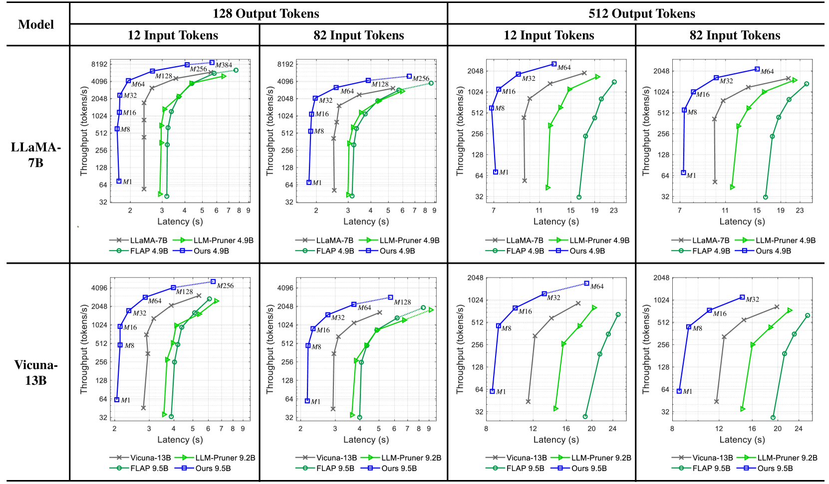Appendix — Shortened LLaMA: Depth Pruning for LLMs ## Appendix A Additional Results of Inference Efficiency ### A.1 Latency-Throughput Trade-Off As shown in Figure 7, our depth pruning achieves a superior latency-throughput trade-off for various sequence lengths of input and output. In contrast, the width pruning of FLAP An et al. (2024) and LLM-Pruner Ma et al. (2023) degrades efficiency results due to GPU-unfriendly weight dimensions Andersch et al. (2019) (e.g., the hidden sizes of FFN are often not divisible by 8). The markers labeled with $M$ represent batch sizes. The dotted lines indicate that pruned models can operate with larger batch sizes, avoiding out-of-memory errors encountered by the original model. <details> <summary>x6.png Details</summary>  ### Visual Description ## [Chart Type]: Throughput vs. Latency for Language Models (LLaMA-7B, Vicuna-13B) and Their Variants ### Overview The image contains 8 line charts (2 rows × 4 columns) comparing **throughput (tokens/s)** vs. **latency (s)** for two base models (LLaMA-7B, Vicuna-13B) and their pruned/optimized variants (LLM-Pruner, FLAP, “Ours”) under different input (12, 82 tokens) and output (128, 512 tokens) lengths. ### Components/Axes - **Y-axis**: Throughput (tokens/s) (logarithmic scale: 32, 64, 128, 256, 512, 1024, 2048, 4096, 8192 for 128 output; 32–2048 for 512 output). - **X-axis**: Latency (s) (linear scale: 2–9 for 128 output; 7–23 for 512 output). - **Legend**: - LLaMA-7B (gray ×), LLM-Pruner 4.9B (green △), FLAP 4.9B (green ○), Ours 4.9B (blue □) (top row). - Vicuna-13B (gray ×), LLM-Pruner 9.2B (green △), FLAP 9.5B (green ○), Ours 9.5B (blue □) (bottom row). - **Data Points**: Labeled with “M1, M8, M16, M32, M64, M128, M256, M384” (likely representing model configurations, e.g., batch size or sequence length). ### Detailed Analysis (Per Chart) #### 1. LLaMA-7B, 128 Output Tokens, 12 Input Tokens - **LLaMA-7B (gray ×)**: Throughput rises with latency, plateauing at ~4096 tokens/s (M64–M384, latency ~4–7s). - **LLM-Pruner 4.9B (green △)**: Throughput rises with latency, plateauing at ~4096 tokens/s (M128–M256, latency ~5.5–6s). - **FLAP 4.9B (green ○)**: Similar to LLM-Pruner (plateau ~4096 tokens/s). - **Ours 4.9B (blue □)**: Throughput rises with latency, reaching ~8192 tokens/s (M384, latency ~7s) – higher than LLaMA-7B. #### 2. LLaMA-7B, 128 Output Tokens, 82 Input Tokens - Trends mirror 12 Input Tokens, with “Ours 4.9B” outperforming LLaMA-7B and pruned models. #### 3. LLaMA-7B, 512 Output Tokens, 12 Input Tokens - **Y-axis max**: 2048 tokens/s (lower than 128 output, as expected for longer outputs). - **LLaMA-7B (gray ×)**: Plateaus at ~2048 tokens/s (M32–M64, latency ~10–11s). - **Ours 4.9B (blue □)**: Matches LLaMA-7B’s throughput at similar latency. #### 4. LLaMA-7B, 512 Output Tokens, 82 Input Tokens - Trends mirror 12 Input Tokens, with “Ours 4.9B” performing comparably to LLaMA-7B. #### 5. Vicuna-13B, 128 Output Tokens, 12 Input Tokens - **Vicuna-13B (gray ×)**: Plateaus at ~4096 tokens/s (M64–M256, latency ~4–6s). - **Ours 9.5B (blue □)**: Matches Vicuna-13B’s throughput at similar latency. #### 6. Vicuna-13B, 128 Output Tokens, 82 Input Tokens - Trends mirror 12 Input Tokens, with “Ours 9.5B” performing comparably to Vicuna-13B. #### 7. Vicuna-13B, 512 Output Tokens, 12 Input Tokens - **Y-axis max**: 2048 tokens/s. - **Vicuna-13B (gray ×)**: Plateaus at ~2048 tokens/s (M32–M64, latency ~11–12s). - **Ours 9.5B (blue □)**: Matches Vicuna-13B’s throughput at similar latency. #### 8. Vicuna-13B, 512 Output Tokens, 82 Input Tokens - Trends mirror 12 Input Tokens, with “Ours 9.5B” performing comparably to Vicuna-13B. ### Key Observations - **Throughput-Latency Tradeoff**: Throughput increases with latency but plateaus (e.g., LLaMA-7B plateaus at 4096 tokens/s for 128 output). - **Output Length Impact**: 128 output tokens enable higher throughput (up to 8192) than 512 output tokens (up to 2048). - **Model Optimization**: “Ours” models (blue □) outperform or match original models (LLaMA-7B, Vicuna-13B) and pruned variants (LLM-Pruner, FLAP) in throughput/latency. - **Pruning Tradeoff**: Pruned models (LLM-Pruner, FLAP) have lower throughput than original models, indicating size reduction (not shown) comes at the cost of inference speed. ### Interpretation This data evaluates model performance in inference scenarios, where **throughput** (processing rate) and **latency** (response time) are critical. Key insights: - Shorter outputs (128 tokens) boost throughput, while longer outputs (512 tokens) reduce maximum throughput but increase latency. - “Ours” models demonstrate effective optimization, achieving higher throughput (or similar throughput with lower latency) than original/pruned models. - Pruned models (LLM-Pruner, FLAP) sacrifice throughput for reduced size, making them less suitable for high-throughput tasks. This analysis helps practitioners choose models based on task requirements (e.g., real-time vs. batch processing) and understand the tradeoffs between model size, speed, and output length. </details> Figure 7: Inference efficiency of pruned models on an NVIDIA H100 GPU. ### A.2 GPU Memory Requirements Table 8 shows the gains in VRAM usage from our pruned models on an NVIDIA H100 given 12 input tokens. The larger the batch size, the greater the improvement observed. Notably, our pruned models can handle an output length of 512 and a batch size of 64, unlike the original 13B-parameter model. #Param $L$ 128 $L$ 512 $M$ 1 $M$ 16 $M$ 64 $M$ 1 $M$ 16 $M$ 64 6.7B (Original) 12.8GB 16.0GB 25.8GB 13.3GB 25.0GB 61.8GB 5.5B (20% Pruned) 10.5GB 13.1GB 21.1GB 10.9GB 20.4GB 50.4GB 4.9B (27% Pruned) 9.4GB 11.6GB 18.8GB 9.7GB 18.1GB 44.6GB 4.5B (35% Pruned) 8.6GB 10.7GB 17.2GB 9.0GB 16.6GB 40.8GB 13.0B (Original) 24.8GB 29.6GB 44.9GB 25.5GB 43.7GB OOM 10.5B (21% Pruned) 19.9GB 23.8GB 36.0GB 20.5GB 35.0GB OOM 9.5B (29% Pruned) 18.1GB 21.7GB 32.7GB 18.6GB 31.8GB 73.5GB 8.3B (37% Pruned) 15.7GB 18.8GB 28.3GB 16.1GB 27.5GB 63.5GB Table 8: GPU memory requirements for varying sequence lengths ( $L$ ) and batch sizes ( $M$ ). The results of the 7B and 13B models and our models with different pruning ratios are reported. Our approach effectively reduces the memory demands of the original models. ## Appendix B Further Results of Moderate Pruning and LoRA Retraining ### B.1 Zero-shot Downstream Task Performance PPL↓ Commonsense Reasoning Accuracy↑ (%) Thr↑ (tokens/s) $‡$ #Param & Method Wiki2 PTB Average BoolQ PIQA HellaSwag WinoGrande ARC-e ARC-c OBQA H100 RTX3090 LLaMA-7B: 6.7B 12.6 22.1 66.3 75.0 78.7 76.2 69.9 75.3 44.7 44.4 53.7 25.0 Wanda-sp 21.4 47.2 51.8 61.5 70.4 53.2 56.0 58.7 31.4 31.0 41.7 16.7 FLAP 17.0 30.1 59.5 69.4 74.7 66.9 66.3 64.6 36.5 38.2 40.5 16.5 LLM-Pruner 17.6 30.4 61.8 66.2 77.6 71.4 66.1 70.5 39.3 41.2 43.2 21.4 SLEB 18.5 31.6 57.6 65.0 75.0 65.7 57.9 67.6 36.6 35.8 66.0 28.4 Ours: Grad+ 20.2 32.3 63.5 75.7 75.7 71.5 69.1 69.9 41.6 40.8 66.0 28.4 5.5B (20% Pruned) Ours: PPL 17.7 30.7 61.9 72.7 75.7 70.4 63.6 69.5 40.1 41.2 66.0 28.4 Wanda-sp 50.4 106.9 42.1 62.0 60.4 33.2 52.8 37.6 23.0 25.4 41.7 16.0 FLAP 21.3 37.1 55.8 68.2 70.6 61.0 64.1 58.8 31.4 36.8 40.2 16.5 LLM-Pruner 20.5 36.1 58.7 62.8 75.5 67.2 64.9 63.5 36.8 40.2 44.0 22.9 SLEB 25.3 41.3 52.6 62.1 71.1 57.2 53.3 57.5 31.6 35.6 73.9 34.9 Ours: Grad+ 29.9 42.0 59.8 70.6 73.0 65.7 68.5 63.9 39.3 37.4 73.9 34.9 4.9B (27% Pruned) Ours: PPL 20.7 36.0 57.6 66.6 73.1 63.7 60.4 64.3 36.0 39.2 73.9 34.9 Wanda-sp 133.6 210.1 36.9 44.5 56.8 29.6 49.6 31.7 20.7 25.6 41.6 16.1 FLAP 25.6 44.4 52.7 68.3 68.1 55.9 61.1 52.3 29.4 33.8 40.5 15.8 LLM-Pruner 24.2 40.7 55.5 62.9 72.8 62.3 62.7 57.4 33.0 37.6 44.4 21.1 SLEB 34.2 49.8 50.1 62.2 69.0 52.7 52.9 51.6 29.9 32.2 80.1 37.8 Ours: Grad+ 33.2 58.5 55.4 62.5 69.2 60.7 66.8 57.4 34.5 36.8 80.1 37.8 4.5B (35% Pruned) Ours: PPL 23.1 38.8 55.2 64.3 71.4 59.4 59.3 62.2 32.8 37.0 80.1 37.8 PPL↓ Commonsense Reasoning Accuracy↑ (%) Thr↑ (tokens/s) $‡$ #Param & Method Wiki2 PTB Average BoolQ PIQA HellaSwag WinoGrande ARC-e ARC-c OBQA H100 RTX3090 Vicuna-7B: 6.7B 17.1 63.2 65.9 78.1 77.3 73.9 69.5 74.3 44.3 43.8 53.7 25.0 Wanda-sp 24.4 104.0 58.5 63.9 72.0 67.4 65.2 64.8 38.3 37.8 41.7 16.7 FLAP 22.0 74.9 61.4 73.1 74.8 67.9 65.8 67.5 40.2 40.6 40.5 16.5 LLM-Pruner 19.6 76.4 60.1 65.4 76.2 68.9 64.4 68.9 37.4 39.4 43.2 21.4 SLEB 25.1 77.0 55.6 63.2 72.1 61.2 59.4 64.3 34.1 35.2 66.0 28.4 Ours: Grad+ 21.0 72.3 62.5 78.7 74.8 69.4 68.5 68.2 38.7 39.6 66.0 28.4 5.5B (20% Pruned) Ours: PPL 18.8 67.9 60.7 71.7 74.4 67.6 63.6 69.3 38.9 39.4 66.0 28.4 Wanda-sp 36.5 177.6 50.9 49.0 67.1 57.2 59.2 57.6 33.7 32.4 41.7 16.0 FLAP 27.9 88.3 57.1 72.0 71.5 62.0 61.2 61.2 35.4 36.6 40.2 16.5 LLM-Pruner 22.7 87.9 57.1 60.8 74.3 65.9 60.9 64.4 34.6 38.8 44.0 22.9 SLEB 34.0 98.0 49.9 47.9 68.7 54.6 56.1 58.4 31.3 32.4 73.9 34.9 Ours: Grad+ 29.8 92.0 60.2 78.8 71.8 64.4 67.7 64.3 36.4 37.6 73.9 34.9 4.9B (27% Pruned) Ours: PPL 23.0 78.2 56.1 66.4 72.9 60.6 59.2 63.1 33.8 37.0 73.9 34.9 Wanda-sp 73.2 386.5 39.4 43.1 58.4 36.3 53.3 34.5 23.7 26.4 41.6 16.1 FLAP 34.6 104.8 53.7 65.1 68.1 57.0 63.1 56.9 32.0 34.0 40.5 15.8 LLM-Pruner 27.6 102.0 53.5 52.0 72.4 61.6 59.9 58.0 33.3 37.0 44.4 21.1 SLEB 43.5 117.3 45.4 41.3 65.9 47.3 51.5 51.6 28.0 32.2 80.1 37.8 Ours: Grad+ 35.0 110.3 55.0 64.0 69.6 59.3 66.5 57.5 33.3 35.2 80.1 37.8 4.5B (35% Pruned) Ours: PPL 26.6 89.4 53.3 65.2 70.4 56.5 56.6 59.8 31.5 33.4 80.1 37.8 PPL↓ Commonsense Reasoning Accuracy↑ (%) Thr↑ (tokens/s) $‡$ #Param & Method Wiki2 PTB Average BoolQ PIQA HellaSwag WinoGrande ARC-e ARC-c OBQA H100 RTX3090 Vicuna-13B: 13.0B 14.7 51.6 68.3 82.8 78.3 77.0 71.2 75.4 47.7 45.4 45.5 OOM Wanda-sp 19.0 71.8 63.6 78.6 75.6 73.5 68.4 68.5 42.2 38.4 34.1 12.9 FLAP 18.8 65.3 63.3 77.2 75.1 72.0 70.2 69.4 40.3 38.8 32.6 12.6 LLM-Pruner 16.0 57.0 65.3 75.5 78.6 75.0 69.8 70.6 43.6 44.4 34.0 17.3 SLEB 20.5 68.7 60.4 71.3 73.4 68.3 63.9 66.8 38.7 40.2 55.7 23.9 Ours: Grad+ 18.1 61.6 66.7 83.0 76.8 75.1 72.8 72.5 44.5 42.4 55.7 23.9 10.5B (21% Pruned) Ours: PPL 16.1 56.5 64.9 75.0 77.1 73.7 68.9 71.5 43.8 44.2 55.7 23.9 Wanda-sp 23.4 84.9 60.0 71.5 74.2 68.7 65.1 64.3 36.8 39.4 33.7 13.5 FLAP 22.8 78.8 61.6 75.9 73.7 67.9 66.4 67.3 38.0 42.0 33.0 12.1 LLM-Pruner 19.0 66.4 62.7 68.3 77.1 72.0 69.7 68.6 40.0 43.4 35.8 15.0 SLEB 26.2 85.0 56.0 61.3 71.4 64.1 59.6 60.0 37.0 38.4 62.0 24.2 Ours: Grad+ 22.0 70.3 65.1 82.6 75.1 73.3 70.9 69.9 43.8 40.2 62.0 24.2 9.5B (29% Pruned) Ours: PPL 18.1 62.2 62.0 67.5 75.6 70.6 65.5 70.9 43.3 40.2 62.0 24.2 Wanda-sp 36.6 123.5 52.7 59.6 67.5 59.5 59.7 55.2 33.5 33.8 33.8 12.6 FLAP 28.7 96.2 58.3 72.5 70.0 62.5 65.4 63.8 36.3 37.8 32.9 13.2 LLM-Pruner 22.2 74.0 59.7 67.1 75.6 67.7 63.2 65.5 38.8 39.8 35.6 18.0 SLEB 41.6 116.5 49.4 47.8 67.8 54.5 56.1 53.8 32.2 33.6 69.7 31.7 Ours: Grad+ 34.2 90.4 61.4 78.5 71.3 69.2 69.9 64.2 40.5 36.6 69.7 31.7 8.3B (37% Pruned) Ours: PPL 22.1 73.6 59.1 69.4 73.8 64.4 62.5 65.1 39.2 39.0 69.7 31.7 $‡$ Throughput measured with 12 input tokens, 128 output tokens, and a batch size of 1 on a single GPU. Table 9: Results of pruned LLaMA-7B (top), Vicuna-7B-v1.3 (middle), and Vicuna-13B-v1.3 (bottom). The width pruning of Wanda-sp Sun et al. (2024); An et al. (2024), FLAP An et al. (2024), and LLM-Pruner Ma et al. (2023) often degrades inference efficiency due to the GPU-unfriendly weight sizes Andersch et al. (2019). In contrast, our depth pruning delivers actual speedups while performing comparably with light LoRA retraining. ### B.2 Generation Examples Tables 10 and 11 present generation examples where some input prompts were sourced from Ma et al. (2023). In terms of linguistic flow and topical consistency, the pruned models yield sentences on par with those from the original model. However, as also noted in Ma et al. (2023), the output quality deteriorates when responding to factual questions or producing longer content. To overcome this challenge, it is essential to apply a more powerful retraining method on a large-scale corpus. Model Generated Text LLaMA-7B What’s great about the holiday season, it’s a time when people focus less on work and more on families and friends. The holidays are a time when people can really focus on giving and helping others, which is something that the holidays are supposed to be about. In my blog post this week, I’ll be taking a look at a variety of causes that … Wanda-sp What’s great about the holiday season, though, is its warm and inviting people, and what a chance to meet and share a cuppa with others who understand and have shared similar experiences, a feeling of empathy if you will, and a great opportunity to help others on a difficult journey. So I can say, all is well. But I’m not giving up the fight … FLAP What’s great about the holiday season, and what makes it such an awesome time of the year, is that it’s the time of the year when people are so generous, and so goodhearted. When you get together with friends and family, and you go through the various things that you’re able to do, when you’re able to give people gifts, when people can see … LLM-Pruner What’s great about the holiday season, is you can enjoy the company of friends and family. This is the perfect opportunity to gather together, and share all the special memories that you have together. These moments are the ones that make the holiday special. No matter what happens, or what you end up doing, it’s always good to get … Ours: Taylor+ What’s great about the holiday season, is that it’s a time of year when people can actually take a step back from the normal day-to-day routines and take some time out to relax and enjoy some well-deserved rest and rejuvenation. This might include indulging in a more comfortable or luxury holiday experience and this article aims to help … Ours: PPL What’s great about the holiday season, in my mind, is that it brings together friends, family, and food. The holiday season is a great time to show some love and have some fun with the people that matter most. Whether you are celebrating Christmas, Hanukah, or New Years, the festivities will be full of joy and memories that will last … LLaMA-7B AI can create a logo in seconds. Why are these new technologies threatening our jobs? AI can do most menial tasks in just a few seconds or minutes. These tasks can be very tedious for human beings to do. For instance, AI can identify patterns in large amounts of data so that complex statistical analysis can be carried out faster than a … Wanda-sp AI can create a logo in seconds rather than years. To this point, this is only the beginning of what AI will do to change our human lives. As time goes on, it’s quite likely that we’ll see even greater use of robots. Even if this all sounds too dramatic, this may still happen. And AI is the best thing that can make it to happen. in 2019. All you … FLAP AI can create a logo in seconds and it doesn’t cost you a penny. The new era of technology has opened up many exciting opportunities. Technology, like AI is being utilized for different purposes in different ways, and now, technology is becoming a solution to problems that would have been tedious or expensive only a few years ago. … LLM-Pruner AI can create a logo in seconds, design a website from scratch and even write blog posts without any human intervention. This revolution is changing the way humans communicate and express ideas. In our view, this technology is a great asset but we’ll need to be smart in how we use it to prevent abuse or automation leading to … Ours: Taylor+ AI can create a logo in seconds or design a new website. There is a lot of software that exists in these two categories. It has become easier and faster for people to use. However, there is still the requirement for the designer or creative director to ensure that the designs are relevant and meaningful to the brand. The Future: AI for creative design … Ours: PPL AI can create a logo in seconds, and it can design entire websites, all without human intervention. However, there is still a lot of work to be done to perfect this technology, including the development of natural language processing, machine learning and computer vision, as well as ensuring that AI designers are creating work that can be … LLaMA-7B Neural network pruning is defined as the process of removing certain weights or neurons in a neural network to reduce the size of the neural network, and improve the training process. Neural networks pruning techniques have been applied successfully on classification, optimization, planning, and speech recognition tasks. A pruned … Wanda-sp Neural network pruning is defined as any method that removes the redundant information by applying the neural network network. It is the term used to identify the systematic variables when an individual tries to find an algorithm. In addition, it is the method of classification used to define any set of algorithms that have been … FLAP Neural network pruning is defined as a selection of neurons or weights in a neural network so that the information of the network is reduced to a specified level, and a process of re-training a neural network. The latter one is the most popular method, especially the neural network pruning. In recent years, this field has been studied in … LLM-Pruner Neural network pruning is defined as reducing the complexity and size of an over-parameterized neural network. The pruning reduces the FLOPs and improves performance for the particular task. Pruning techniques have gained popularity in recent years due to their wide range of applications. This paper aims to explore the pruning … Ours: Taylor+ Neural network pruning is defined as reducing the weight connections and biases of a neural network, while retaining high performance. Pruning is an effective approach to reducing the number of parameters and improving the efficiency of neural networks. Recently, the concept of neural network shrinking has gained considerable … Ours: PPL Neural network pruning is defined as the process of removing redundant neurons and connections between nodes in a neural network, while keeping the performance or accuracy to the maximum extent possible. This optimization is aimed at reducing the size and memory consumption of the network while maintaining its ability to perform task … Table 10: Generation examples from the original LLaMA-7B and 20%-compressed models. Model Generated Text Vicuna-13B What’s great about the holiday season, beyond the obvious time off and the chance to spend time with loved ones, is the opportunity to slow down and reflect on the year that’s passed. It’s a time to look back at all the accomplishments and growth you’ve experienced, and to set your sights on the year ahead. As a small business owner, the … Wanda-sp What’s great about the holiday season, besides spending time with family and friends, is that it’s a time of giving. It’s a time to show appreciation for those in your life who make a difference and bring joy to your world. Whether it’s a gift of love, a gift of time, or a gift of money, it’s important to remember that giving is not just about … FLAP What’s great about the holiday season, especially the days leading up to Christmas, is the opportunity to take a pause and recharge. It’s a time to reflect on the year and all the experiences we’ve had, good or bad. It’s a time to reflect on the people we love and the impact they’ve had on our lives. It’s a time to reflect on what we want … LLM-Pruner What’s great about the holiday season, aside from the gifts and the holiday parties, is the opportunity to spend time with family and loved ones. One of the things that I love most about holiday seasons is the traditions that surround them, from decorating the tree to making special holiday meals, there’s a sense of nostalgia and warmth that … Ours: Taylor+ What’s great about the holiday season, is that it allows us to reflect on the year gone by and reflect on the moments that made it special. And while some people might choose to celebrate with the traditional traditions, some choose to do something different. One way to spice up your holiday season is by taking a trip to a far-off place. Why not … Ours: PPL What’s great about the holiday season, in addition to the fun food, festivities, and spending time with loved ones, is that it creates the perfect opportunity to show people how much you appreciate them. From giving them a gift, to baking their favorite treat, or just taking a moment to acknowledge them in front of others – there’s something … Vicuna-13B AI can create a logo in seconds with its complex algorithms and pre-set designs. But it can never truly understand the essence of a business, the emotions that go into creating a logo or the creativity and uniqueness that comes from human input. It’s time to put the human touch back into branding, where a designer and client can collaborate to … Wanda-sp AI can create a logo in seconds using a logo design tool. However, a talented graphic designer can create a unique and meaningful logo that stands out from the crowd, captures the essence of the business, and appeals to the target audience. A good logo can also make a difference in how customers perceive the business and can even increase … FLAP AI can create a logo in seconds. If you don’t like it, you can change it yourself or pay for a designer to do it for you. However, it’s important to note that a logo is more than just an image. It’s a visual representation of a brand or organization, and it communicates certain values and characteristics to the viewer. Therefore, it’s essential to … LLM-Pruner AI can create a logo in seconds with just one click, but design is a human art, something that is beyond AI capabilities. The logo design is an important part of a company’s identity, and it’s a decision that affects the company’s visual branding and reputation for years to come. The logo is the visual representation of a company’s values … Ours: Taylor+ AI can create a logo in seconds, with or without a human’s input. Some people might like this, because they can create a logo for a small business on a budget. Other people, like myself, think that the human touch is important in art and design. A human designer can create a unique and meaningful logo by incorporating personal … Ours: PPL AI can create a logo in seconds by combining a variety of different styles and shapes and patterns that make up the logos. However, a logo that is truly a reflection of your brand needs to be designed by a human, a graphic designer. They will bring a creative vision that will make your logo unique, appealing and memorable. They can add … Vicuna-13B Neural network pruning is defined as the process of removing redundant or unnecessary connections in a neural network to reduce its size and computational complexity while preserving its performance. The primary motivation behind pruning is to improve the efficiency of deep learning models, especially in resource-constrained … Wanda-sp Neural network pruning is defined as a method for removing connections in order to reduce the model size, thus allowing for computationally efficient models while retaining accuracy. This technique is useful in reducing the number of neurons in a neural network, which allows for fewer computations during training and reduces the … FLAP Neural network pruning is defined as the process of reducing the size of a neural network by removing the least significant weights or neurons. The main motivation for pruning is to reduce the computational cost of neural networks while maintaining their accuracy. The key challenge of pruning is to identify the most effective … LLM-Pruner Neural network pruning is defined as a technique that aims to reduce the size of a neural network by removing redundant and irrelevant connections between the neurons in the network. This approach is based on the observation that a large portion of the connections within the network is redundant and does not contribute to the overall … Ours: Taylor+ Neural network pruning is defined as the removal of redundant connections within a neural network to achieve a better model fit while retaining the network’s general accuracy. The goal of pruning is to reduce the computational cost and memory footprint of the network. One commonly used pruning method is called weight magnitude … Ours: PPL Neural network pruning is defined as the task of removing unnecessary or redundant connections in a neural network while retaining its accuracy and performance. This is often done to reduce the memory usage and computational complexity of a neural network, which can be critical when running on devices with limited resources. In … Table 11: Generation examples from the original Vicuna-13B-v1.3 and 21%-compressed models. ## Appendix C Further Results of Aggressive Pruning and CPT Retraining Figure 8 illustrates the learning curve for models pruned from Vicuna-7B. For each model size, retraining is performed within a two-week span using eight NVIDIA H100 GPUs. The CPT of the 5.5B-parameter model shows early convergence, completing in just 6 days while processing 37B tokens, potentially owing to significant knowledge retained within the network. In contrast, the CPTs for the 3.7B, 2.7B, and 1.5B models take 8, 12, and 11 days, respectively, to process 74B, 150B, and 271B tokens. This process allows the models to restore lost capabilities while achieving improved inference efficiency. Longer training periods could further enhance the recovery of model quality. 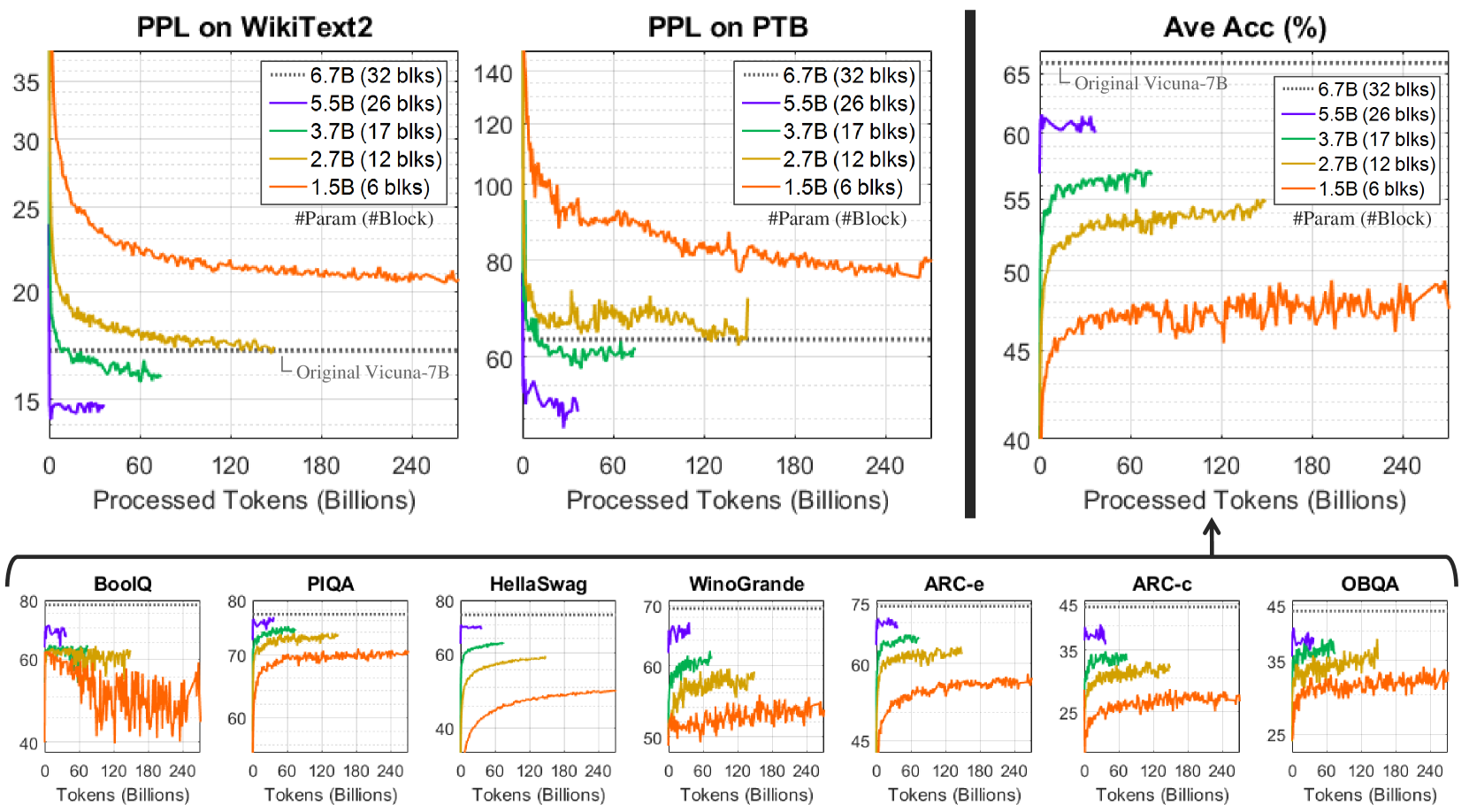<details> <summary>x7.png Details</summary>  ### Visual Description ## [Chart Type]: Model Performance (PPL & Accuracy) Across Datasets and Model Sizes ### Overview The image contains **10 line charts** (3 top, 7 bottom) analyzing model performance (Perplexity, PPL; and Accuracy) as a function of *Processed Tokens (Billions)*. Models are differentiated by parameter count (e.g., 1.5B, 2.7B, 3.7B, 5.5B, 6.7B) with color-coded lines. The “Original Vicuna-7B” (dotted line) serves as a baseline. ### Components/Axes #### Top Charts (3): - **Left: PPL on WikiText2** - Y-axis: PPL (15–35, lower = better). - X-axis: Processed Tokens (0–240 Billions). - Legend: 6.7B (32 blks, dotted), 5.5B (26 blks, purple), 3.7B (17 blks, green), 2.7B (12 blks, yellow), 1.5B (6 blks, orange). - Baseline: “Original Vicuna-7B” (dotted line, ~17 PPL). - **Middle: PPL on PTB** - Y-axis: PPL (60–140, lower = better). - X-axis: Processed Tokens (0–240 Billions). - Legend: Same as left. - Baseline: “Original Vicuna-7B” (dotted line, ~60 PPL). - **Right: Ave Acc (%)** - Y-axis: Accuracy (40–65%, higher = better). - X-axis: Processed Tokens (0–240 Billions). - Legend: Same as left. - Baseline: “Original Vicuna-7B” (dotted line, ~65%). #### Bottom Charts (7 Datasets): Each chart plots accuracy (Y-axis, varying ranges) vs. Processed Tokens (X-axis, 0–240 Billions). Datasets: *BoolQ, PIQA, HellaSwag, WinoGrande, ARC-e, ARC-c, OBQA*. Same model legend (colors: purple=5.5B, green=3.7B, yellow=2.7B, orange=1.5B; dotted=6.7B). ### Detailed Analysis #### Top Left: PPL on WikiText2 - **Trend:** All models show *decreasing PPL* (improved performance) with more tokens. - 1.5B (orange): Starts ~35, drops to ~20 (240B tokens). - 2.7B (yellow): Starts ~25, drops to ~17. - 3.7B (green): Starts ~20, drops to ~16. - 5.5B (purple): Starts ~15, remains flat (~15). - 6.7B (dotted): Flat at ~17 (matches “Original Vicuna-7B”). #### Top Middle: PPL on PTB - **Trend:** Similar to WikiText2, but *higher PPL* (PTB is a harder dataset). - 1.5B (orange): Starts ~140, drops to ~80. - 2.7B (yellow): Starts ~100, drops to ~70. - 3.7B (green): Starts ~80, drops to ~60. - 5.5B (purple): Starts ~60, drops to ~50. - 6.7B (dotted): Flat at ~60 (matches “Original Vicuna-7B”). #### Top Right: Ave Acc (%) - **Trend:** All models show *increasing accuracy* with more tokens. - 1.5B (orange): Starts ~40, rises to ~50. - 2.7B (yellow): Starts ~50, rises to ~55. - 3.7B (green): Starts ~55, rises to ~57. - 5.5B (purple): Starts ~60, rises to ~62. - 6.7B (dotted): Flat at ~65 (matches “Original Vicuna-7B”). #### Bottom Charts (7 Datasets) - **BoolQ:** Y-axis (40–80). 1.5B (orange) has high variance; others (purple, green, yellow) are stable. All increase with tokens. - **PIQA:** Y-axis (60–80). 1.5B (orange) starts ~60, rises to ~70. Larger models (purple, green, yellow) start ~70–80 (stable). - **HellaSwag:** Y-axis (40–80). 1.5B (orange) starts ~40, rises to ~50. Larger models start ~60–70 (stable). - **WinoGrande:** Y-axis (50–70). 1.5B (orange) starts ~50, rises to ~55. Larger models start ~60–65 (stable). - **ARC-e:** Y-axis (45–75). 1.5B (orange) starts ~45, rises to ~55. Larger models start ~60–70 (stable). - **ARC-c:** Y-axis (25–45). 1.5B (orange) starts ~25, rises to ~35. Larger models start ~35–40 (stable). - **OBQA:** Y-axis (25–45). 1.5B (orange) starts ~25, rises to ~35. Larger models start ~35–40 (stable). ### Key Observations 1. **Model Size vs. Performance:** Larger models (more parameters) have *better initial performance* (lower PPL, higher accuracy) and improve more consistently with tokens. 2. **Dataset Difficulty:** PPL on PTB is higher than WikiText2, indicating PTB is a harder language modeling dataset. 3. **Training Progress:** All models show improvement (lower PPL, higher accuracy) with more tokens, confirming continued learning. 4. **Baseline Comparison:** “Original Vicuna-7B” (dotted line) is matched/exceeded by larger models (6.7B) and smaller models with more tokens. ### Interpretation The charts illustrate the critical role of **model size** (parameter count) and **training tokens** in improving language modeling (PPL) and question-answering/reading comprehension (accuracy). Larger models (e.g., 6.7B) outperform smaller ones (e.g., 1.5B) initially and maintain stability, while smaller models require more tokens to approach baseline performance. This suggests: - Scaling model size (parameters) and training data (tokens) are complementary strategies for performance gains. - Diminishing returns exist for very large models (e.g., 5.5B and 6.7B have similar trends). - Smaller models (1.5B) are less stable (high variance) but still benefit from more training. These insights guide decisions on model architecture and training duration for real-world NLP tasks. </details> Figure 8: Zero-shot performance over the course of training for models from Vicuna-7B-v1.3 at different pruning ratios. For each model size, the CPT duration was limited to a two-week period, but additional training could further improve the quality. ## Appendix D Compatibility with PTQ Our pruning approach can be combined with quantization to further decrease memory usage. To validate this aspect, we apply 4-bit GPTQ Frantar et al. (2023) to our pruned models, using 128 randomly sampled sequences with 2048 tokens from the C4 dataset Raffel et al. (2020) as calibration data for PTQ. The results demonstrate that quantization does not cause a noticeable degradation in zero-shot model performance while leading to additional computational reductions. ### D.1 Zero-shot Performance after Applying Quantization Model PPL ↓ Commonsense Reasoning Accuracy↑ (%) #Param Retraining Quantization Wiki2 PTB Average BoolQ PIQA HellaSwag WinoGrande ARC-e ARC-c OBQA 6.7B (Original) - ✗ 17.1 63.2 65.9 78.1 77.3 73.9 69.5 74.3 44.3 43.8 ✓ 17.3 64.8 63.6 72.5 76.4 72.4 67.6 72.8 42.7 40.4 5.5B (20% Pruned) LoRA ✗ 18.8 67.9 60.7 71.7 74.4 67.6 63.6 69.3 38.9 39.4 ✓ 19.7 70.7 60.1 70.2 74.6 66.9 64.4 67.6 38.6 38.4 CPT ✗ 14.3 56.2 61.5 70.5 75.7 69.9 65.7 70.4 39.2 39.2 ✓ 15.1 59.3 60.6 69.7 75.9 68.9 63.9 68.5 38.5 38.6 CPT $⇒$ LoRA ✗ 14.8 60.2 63.1 72.5 77.5 71.1 66.0 72.1 41.1 41.0 ✓ 15.5 64.1 61.7 71.1 76.4 70.3 64.2 71.5 40.9 37.6 3.7B (45% Pruned) LoRA ✗ 37.0 113.2 47.0 54.3 67.1 45.3 53.4 52.2 27.6 28.8 ✓ 38.0 117.6 46.8 55.3 66.2 45.1 53.5 50.5 27.6 29.2 CPT ✗ 16.0 60.0 57.1 62.6 74.5 63.5 62.4 66.0 34.4 36.4 ✓ 16.6 61.5 57.1 63.8 74.5 62.7 61.0 65.8 34.2 37.8 CPT $⇒$ LoRA ✗ 16.5 60.5 57.4 62.0 74.9 64.8 61.7 65.2 34.1 39.0 ✓ 17.0 61.8 56.9 61.0 74.5 64.1 61.8 64.7 34.1 38.4 2.7B (60% Pruned) LoRA ✗ 68.9 196.4 40.1 41.3 61.0 33.9 53.0 40.4 25.2 26.0 ✓ 71.5 205.9 40.1 42.7 60.4 33.7 52.6 40.7 24.9 25.8 CPT ✗ 17.1 63.1 55.0 61.8 73.5 58.6 58.2 62.4 31.8 38.6 ✓ 17.7 64.7 54.6 61.9 73.1 58.4 58.8 62.5 31.8 35.6 CPT $⇒$ LoRA ✗ 17.8 65.1 55.0 61.4 73.9 59.7 58.0 61.3 32.3 38.0 ✓ 18.4 66.1 55.0 61.9 73.8 59.0 58.3 62.1 32.0 38.0 1.5B (80% Pruned) LoRA ✗ 1002.2 1874.9 37.1 51.6 53.5 26.4 49.3 27.8 27.5 24.0 ✓ 1014.3 1932.4 37.5 53.7 53.3 26.5 50.0 28.2 26.5 24.6 CPT ✗ 20.5 77.4 49.2 53.5 70.7 48.9 54.5 56.7 27.0 33.0 ✓ 21.4 80.0 48.5 48.9 70.1 48.8 54.1 55.7 26.8 35.0 CPT $⇒$ LoRA ✗ 21.1 79.0 49.0 52.5 70.7 49.6 52.7 55.6 28.0 34.0 ✓ 21.8 82.0 48.6 51.7 70.2 49.8 52.7 55.0 27.6 33.4 Table 12: Zero-shot results from applying PTQ to various pruned and retrained models derived from Vicuna-7B-v1.3. ### D.2 Further GPU Memory Reduction from Quantization Model $L$ 128 $L$ 512 # Param Quantization $M$ 1 $M$ 16 $M$ 64 $M$ 256 $M$ 1 $M$ 16 $M$ 64 $M$ 256 6.7B (Original) ✗ 12.8GB 16.0GB 25.8GB 65.0GB 13.3GB 25.0GB 61.8GB OOM ✓ 4.8GB 7.8GB 17.7GB 56.9GB 5.3GB 16.9GB 53.7GB OOM 5.5B (20% Pruned) ✗ 10.5GB 13.1GB 21.1GB 52.9GB 10.9GB 20.4GB 50.4GB OOM ✓ 4.1GB 6.6GB 14.7GB 46.5GB 4.5GB 14.0GB 43.9GB OOM 3.7B (45% Pruned) ✗ 7.1GB 8.7GB 14.0GB 34.9GB 7.4GB 13.5GB 33.2GB OOM ✓ 3.1GB 4.8GB 10.1GB 31.0GB 3.4GB 9.6GB 29.2GB OOM 2.7B (60% Pruned) ✗ 5.1GB 6.3GB 10.1GB 24.9GB 5.3GB 9.7GB 23.6GB OOM ✓ 2.6GB 3.8GB 7.5GB 22.3GB 2.8GB 7.2GB 21.0GB 76.4GB 1.5B (80% Pruned) ✗ 2.8GB 3.4GB 5.4GB 12.9GB 2.9GB 5.1GB 12.1GB 39.9GB ✓ 1.9GB 2.5GB 4.5GB 12.0GB 2.0GB 4.2GB 11.2GB 39.0GB Table 13: VRAM reduction by applying quantization after using our pruning method. The results of the pruned Vicuna-7B models and their 4-bit weight-quantized counterparts are reported under varying sequence lengths ( $L$ ) and batch sizes ( $M$ ). ## Appendix E Experimental Setup ### E.1 Baseline Methods We primarily compare the two pruning units, focusing on ‘network width vs. depth,’ and also include a very recent depth pruning method in our analysis. The baseline methods are described below, where we use their official code for implementation. To ensure a fair comparison, we employ the same calibration dataset across all methods. Table 14 shows the pruned architectures under similar numbers of parameters. 1. LLM-Pruner (Ma et al., 2023) employs a Taylor-based importance metric to remove attention heads from MHA and intermediate neurons from FFN. Local pruning is performed to select removable groups within the same module while maintaining uniform dimensions across the examined blocks. Adhering to their practice, the first and last few blocks remain unpruned. Their pruned models and ours are identically retrained with LoRA. 1. FLAP (An et al., 2024) uses a fluctuation-based importance metric to explore the recoverability of feature maps after removing weight columns. Global pruning is applied, leading to different widths over distinct modules (see Table 14 for mean and standard deviation values). Instead of retraining, extra bias terms are added into pruned feature maps for performance restoration. 1. Wanda-sp is presented in An et al. (2024) as a variant of Wanda (Sun et al., 2024) adjusted for structured pruning. The original metric was based on the product of weight magnitudes and input activation norms, which can be interpreted as addressing a local reconstruction objective. Wanda-sp extends this in a structured way while using common dimensions among different modules. 1. SLEB Song et al. (2024) prunes Transformer blocks in LLMs and has been introduced concurrently with our study. It uses a logit-based method to find unnecessary blocks, similar to our PPL criterion, and updates the importance scores after each block is removed. Although SLEB pursues a retraining-free setup, we observed that it fails to sustain adequate performance as the pruning ratio increases. ### E.2 Implementation Details Our implementation employs the Transformers library Wolf et al. (2020). An NVIDIA A100 (80GB VRAM) GPU is used for the pruning and LoRA retraining phases. For CPT retraining, eight NVIDIA H100 (80GB) GPUs are utilized, with each model size trained in under two weeks. 1. At the pruning phase, we assess the significance of Transformer blocks using a small calibration set (containing 10 samples from BookCorpus (Zhu et al., 2015) with a sequence length of 128). For the PPL-based criterion, the calibration samples are fed into networks with a single block removed, and this step is iterated across all the blocks in the target model. For the Taylor+ method, we feed the calibration data into the original network to collect backward-gradient matrices. The pruning is completed efficiently within 1 to 2 hours for the 7B- and 13B-sized models. 1. At the LoRA retraining phase, we apply a LoRA adapter (Hu et al., 2022) to every projection weight matrix by following Ma et al. (2023). We employ a LoRA rank of 8, a learning rate of 0.0001, and a batch size of 64 over 2 epochs. The retraining costs are notably low, with the entire process being executed on a single GPU. For example, retraining a 20%-pruned model from 7B parameters takes about 2 hours and utilizes 22GB GPU memory, while a 21%-pruned model from 13B parameters requires approximately 3 hours and 35GB VRAM. 1. At the CPT retraining phase, we utilize the AdamW optimizer with ( $β_1$ , $β_2$ ) values of (0.9, 0.95), under a weight decay of 0.1 and a learning rate of 0.0001. A global batch size of 512 is used, with a micro-batch size of 2 for 32 gradient accumulation steps over 8 GPUs. Gradient clipping with a max norm value of 1 is applied. The CPT for the 5.5B-parameter model takes only 6 days (covering 37B tokens) due to early convergence. On the other hand, the CPT for the 3.7B, 2.7B, and 1.5B models takes 8 days (74B tokens), 12 days (150B tokens), and 11 days (271B tokens), respectively. Due to constrained resources, we restricted our CPT procedure to not exceed two weeks for each model size; however, extending the training duration could further improve performance. 1. At the inference stage, we maintain the default configuration of the Transformers library, without using xFormers-optimized attention or advanced options. Model #Param #Block $‡$ #Head $‡$ FFN-D $‡$ Original 7B 6.7B 32 32 11008 20% Pruned $†$ Wanda-sp 5.5B 32 26 8807 FLAP 5.4B 32 26.9±7.5 8577.4±2078.4 LLM-Pruner 5.4B 32 24 8256 Ours 5.5B 26 32 11008 27% Pruned $†$ Wanda-sp 4.9B 32 23 7816 FLAP 4.9B 32 24.6±8.6 7497.1±2358.0 LLM-Pruner 4.9B 32 21 7155 Ours 4.9B 23 32 11008 35% Pruned $†$ Wanda-sp 4.5B 32 21 7156 FLAP 4.5B 32 23.0±8.8 6781.1±2440.6 LLM-Pruner 4.4B 32 18 6054 Ours 4.5B 21 32 11008 45% Pruned $†$ Wanda-sp 3.7B 32 17 5835 FLAP 3.7B 32 18.9±8.0 5506.8±2444.7 LLM-Pruner 3.7B 32 14 4513 Ours 3.7B 17 32 11008 60% Pruned $†$ Wanda-sp 2.7B 32 12 4128 FLAP 2.7B 32 12.7±5.2 4083.6±2359.1 LLM-Pruner 2.7B 32 8 2421 Ours 2.7B 12 32 11008 80% Pruned $†$ Wanda-sp 1.5B 32 6 2059 FLAP 1.5B 32 6.7±2.5 1988.2±852.0 LLM-Pruner 1.5B 32 1 11 Ours 1.5B 6 32 11008 Model #Param #Block $‡$ #Head $‡$ FFN-D $‡$ Original 13B 13.0B 40 40 13824 21% Pruned $†$ Wanda-sp 10.5B 40 32 11060 FLAP 10.5B 40 33.7±8.9 10778.7±2316.0 LLM-Pruner 10.3B 40 30 10368 Ours 10.5B 32 40 13824 29% Pruned $†$ Wanda-sp 9.5B 40 29 9954 FLAP 9.5B 40 31.1±10.6 9570.8±2601.0 LLM-Pruner 9.2B 40 26 8985 Ours 9.5B 29 40 13824 37% Pruned $†$ Wanda-sp 8.4B 40 26 8710 FLAP 8.3B 40 27.5±11.3 8326.6±2874.9 LLM-Pruner 8.2B 40 22 7603 Ours 8.3B 25 40 13824 $†$ Reduction ratio for the number of parameters. $‡$ #Block: #Transformer blocks; #Head: #attention heads of MHA; FFN-D: intermediate size of FFN. Table 14: Pruned architectures on LLaMA-7B and Vicuna-{7B, 13B}-v1.3. While Wanda-sp Sun et al. (2024); An et al. (2024), FLAP An et al. (2024), and LLM-Pruner Ma et al. (2023) reduce the network width, our method reduces the network depth. For moderate pruning ratios under 40%, we used the parameter numbers from LLM-Pruner’s module-level removal ratios of 25%, 35%, and 45% as references and adjusted the pruning ratios for our method and the other baselines.