# A Survey on Transformer Compression
**Authors**: Yehui Tang, Yunhe Wang, Jianyuan Guo, Zhijun Tu, Kai Han, Hailin Hu, and Dacheng Tao
> Yehui Tang, Jianyuan Guo, Zhijun Tu, Kai Han, Hailin Hu, and Yunhe Wang are with Huawei Noah’s Ark Lab. E-mail: Dacheng Tao is with the School of Computer Science, in the Faculty of Engineering, at The University of Sydney, 6 Cleveland St, Darlington, NSW 2008, Australia. E-mail: Corresponding to Yunhe Wang and Dacheng Tao.
## Abstract
Transformer plays a vital role in the realms of natural language processing (NLP) and computer vision (CV), specially for constructing large language models (LLM) and large vision models (LVM). Model compression methods reduce the memory and computational cost of Transformer, which is a necessary step to implement large language/vision models on practical devices. Given the unique architecture of Transformer, featuring alternative attention and feedforward neural network (FFN) modules, specific compression techniques are usually required. The efficiency of these compression methods is also paramount, as retraining large models on the entire training dataset is usually impractical. This survey provides a comprehensive review of recent compression methods, with a specific focus on their application to Transformer-based models. The compression methods are primarily categorized into pruning, quantization, knowledge distillation, and efficient architecture design (Mamba, RetNet, RWKV, etc). In each category, we discuss compression methods for both language and vision tasks, highlighting common underlying principles. Finally, we delve into the relation between various compression methods, and discuss further directions in this domain.
Index Terms: Model Compression, Transformer, Large Language Model, Large Vision Model, LLM
## 1 Introduction
Deep neural networks have become indispensable in numerous artificial intelligence applications, with architectures encompassing diverse formulations, such as multilayer perceptron (MLP), convolutional neural network (CNN), recurrent neural network (RNN), long short-term memory (LSTM), Transformers, etc. In recent times, Transformer-based models have emerged as the prevailing choice across various domains, including both natural language processing (NLP) and computer vision (CV) domains. Considering their strong scalability, most of the large models with over billions of parameters are based on the Transformer architecture, which are considered as foundational elements for artificial general intelligence (AGI) [1, 2, 3, 4, 5, 6].
While large models have demonstrated significant capabilities, their exceptionally vast sizes pose challenges for practical development. For instance, the GPT-3 model has 175 billion parameters and demands about 350GB memory model storage (float16). The sheer volume of parameters and the associated computational expenses necessitate devices with exceedingly high memory and computational capabilities. Directly deploying such models will incur substantial resource costs and contributes significantly to carbon dioxide emissions. Moreover, on edge devices like mobile phones, the development of these models becomes impractical due to the limited storage and computing resources of such devices.
<details>
<summary>x1.png Details</summary>
### Visual Description
## Bar Chart and Flow Diagram: Publications on Transformers and Their Development
### Overview
This image presents two distinct but related sections. The left section is a bar chart showing the number of publications based on Transformers over the years from 2017 to 2023. The right section is a flow diagram illustrating the progression from various model types and applications to large Transformer-based models, followed by compression techniques, and finally, implementation on different devices.
### Components/Axes
**Bar Chart:**
* **Title:** "Number of publications based on Transformers"
* **Y-axis Title:** "# Publications"
* **Y-axis Scale:** Ranges from 0 to 50,000, with major tick marks at 0, 10,000, 20,000, 30,000, 40,000, and 50,000.
* **X-axis Title:** "Year"
* **X-axis Markers:** 2017, 2018, 2019, 2020, 2021, 2022, 2023.
**Flow Diagram:**
* **Input Categories (Left):**
* Ovals containing: "RNN", "NLP", "CV", "CNN", "MLP". Arrows point from these towards "Large Transformer-Based Models".
* **Intermediate Stage:**
* A large oval labeled "Large Transformer-Based Models" containing text: "ChatGPT, LLaMA, BERT, CLIP, ViT...".
* **Compression Techniques (Middle):**
* A list of techniques with arrows pointing from "Large Transformer-Based Models" to them, and then to "Implementation":
* "Pruning"
* "Quantization"
* "Knowledge Distillation"
* "Efficient Architecture"
* "..." (ellipsis indicating more techniques)
* "Compression" (positioned below the ellipsis, suggesting it's a broader category or a related concept).
* **Output Stage (Right):**
* Icons representing implementation:
* A cloud icon with connected squares, representing cloud-based implementation.
* A smartphone icon.
* A desktop computer icon.
* A label below these icons: "Implementation".
### Detailed Analysis or Content Details
**Bar Chart Data:**
The bar chart displays the following approximate publication counts for each year:
* **2017:** Approximately 1,000 publications.
* **2018:** Approximately 2,000 publications.
* **2019:** Approximately 8,000 publications.
* **2020:** Approximately 22,000 publications.
* **2021:** Approximately 42,000 publications.
* **2022:** Approximately 42,000 publications.
* **2023:** Approximately 38,000 publications.
**Flow Diagram Progression:**
The flow diagram illustrates a conceptual pathway:
1. **Foundation Models/Applications:** Traditional model types and application areas like RNN, NLP, CV, CNN, and MLP are shown as inputs that contribute to or are related to the development of Transformer models.
2. **Emergence of Large Transformer Models:** These foundational elements lead to the development of significant Transformer-based models, exemplified by names like ChatGPT, LLaMA, BERT, CLIP, and ViT.
3. **Optimization and Efficiency:** To make these large models practical, various compression and efficiency techniques are applied, including Pruning, Quantization, Knowledge Distillation, and the development of Efficient Architectures. The ellipsis and "Compression" label suggest this is a multifaceted area.
4. **Deployment:** The final stage is "Implementation," depicted by icons for cloud, mobile, and desktop/server environments, indicating the diverse platforms where these optimized Transformer models can be deployed.
### Key Observations
* **Exponential Growth in Publications:** The bar chart clearly shows a dramatic increase in the number of publications related to Transformers, particularly from 2019 to 2021, indicating a surge in research and development in this area.
* **Peak and Slight Decline:** While publications peaked around 2021-2022, there's a slight decrease in 2023, which could be a temporary fluctuation or an indication of a maturing research field or a shift in focus.
* **Interconnectedness of AI Fields:** The flow diagram highlights how older AI paradigms (RNN, CNN, MLP) and application domains (NLP, CV) paved the way for or are integrated with the rise of Transformer models.
* **Focus on Practicality:** The inclusion of compression techniques underscores the ongoing effort to make powerful Transformer models more efficient and deployable across various hardware and software environments.
### Interpretation
The image effectively communicates the trajectory of Transformer-based models in artificial intelligence. The bar chart quantifies the explosive growth in research interest and output concerning Transformers, demonstrating their significant impact on the AI landscape. The rapid ascent from 2019 to 2021 suggests a paradigm shift driven by the capabilities of these models.
The flow diagram provides a conceptual framework for understanding the evolution and application of Transformers. It suggests that while foundational AI concepts and models were crucial, the advent of large Transformer architectures like BERT and GPT has revolutionized the field. The subsequent emphasis on compression and efficient implementation highlights the practical challenges and ongoing innovations required to translate these powerful models into real-world applications across diverse platforms, from cloud services to personal devices. The diagram implies a progression from theoretical development and model creation to optimization and widespread deployment, reflecting the maturity and impact of Transformer technology. The slight dip in publications in 2023, while needing further context, could indicate a stabilization after rapid growth or a transition to more applied research and deployment rather than foundational exploration.
</details>
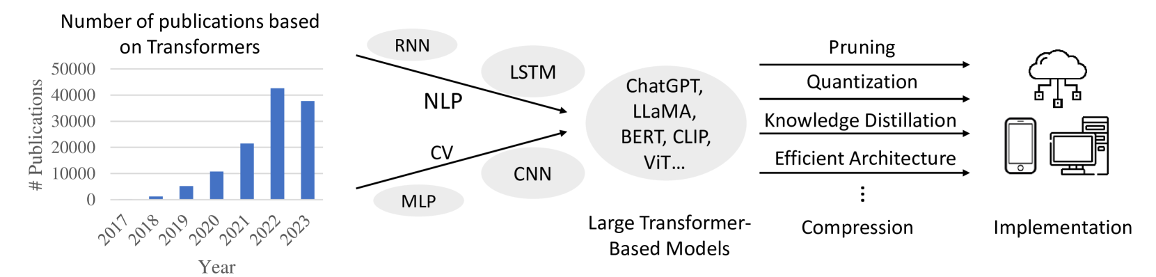
Figure 1: Transformer-based models have emerged as the predominant architectures in both natural language processing (NLP) and computer vision (CV) domains, resulting in a surge in publications. As these models tend to possess substantial dimensions, it becomes imperative to compress their parameters and streamline computational redundancies. This compression is essential for facilitating efficient implementation on practical platforms, ensuring the feasibility of deploying Transformer models in real-world applications.
Model compression is an effective strategy for mitigating the development costs associated with Transformer models. This approach, grounded in the principle of reducing redundancy, encompasses various categories, including pruning, quantization, knowledge distillation, efficient architecture design, etc. Network pruning directly removes redundant components, such as blocks, attention heads, FFN layers, and individual parameters. Diverse sub-models can be derived by employing different pruning granularity and pruning criteria. Quantization reduces the development cost by representing model weights and intermediate features with lower bits. For example, when quantizing a full-precision model (float32) into 8-bit integers, the memory cost can be reduced by a factor of four. According the computational process, it can be divided into post-training quantization(PTQ) or quantization-aware training (QAT), in which the former incurs only limited training costs and is more efficient for large models. Knowledge distillation serves as a training strategy, and transfers knowledge from a large model (teacher) to a smaller model (student). The student mimics the behavior of the teacher by emulating the model’s output and intermediate features. Notably, for advanced models like GPT-4, accessible only through APIs, their generated instructions and explanations can also guide the learning of the student model [7, 8].In addition to obtaining models from predefined large models, some methods yield efficient architectures by directly reducing the computational complexity of attention modules or FFN modules. Combining different methods enables extreme compression. For instance, Han et al. [9] combined network pruning, quantization, and Huffman coding to achieve an impressive 49 $\times$ compression rate on a conventional VGGNet [10].
Regarding Transformer models, their compression strategies exhibit distinct characteristics. Unlike other architectures such as CNN or RNN, the Transformer features a unique design with alternative attention and FFN modules. The former captures the global information by calculating the attention map over different tokens while the latter extracts information from each token respectively. This specific architecture can enable a tailored compression strategy for optimal compression rates. What’s more, the efficiency of compression method becomes especially important for such large models. Due to the high computational cost of large model, it is usually unaffordable to retrain the whole model on the original training set. Some training-efficient methods like post-training compression are preferable.
In this survey, we aim to comprehensively investigate how to compress these Transformer models (Figure 1), and categorize the methods by quantization, knowledge distillation, pruning, efficient architecture design, etc. In each category, we investigate the compression methods for NLP and CV domains, respectively. Table I summarizes the main compression categories and lists representative method suitable for large Transformer models. Though NLP and CV are usually treated as very different domains, we observe that their models compression methods actually share the similar principles. Finally, we discuss the relationship between different compression methods and outline some future research directions.
The rest of the paper is organized as follows. Section 2 introduces the fundamental concept of Transformers. Following this, Section 3 provides an in-depth discussion on compression methods that preserve the architecture, encompassing quantization and knowledge distillation—techniques that maintain the model’s architecture. Section 4 delves further into architecture-preserving compression, including pruning and efficient architecture design. Additional Transformer compression methods are explored in Section 5. Finally, Section 6 draws conclusions on the compression methods and discusses future research directions.
## 2 Concept of Transformer
The Transformer architecture is firstly proposed to tackle tasks like machine translation [11]. A standard Transformer architecture contains main blocks, multi-head attention (MHA) and feed-forward networks (FFN). The attention is formulated as
$$
\mathrm{Attention}(Q,K,V)=\mathrm{softmax}(\frac{QK^{T}}{\sqrt{d}})V, \tag{1}
$$
where $Q$ , $K$ , $V$ are query, key and value matrix, respectively. $d$ is the feature’s dimension. The multi-head attention jointly extracts information from diverse subspaces, which is the concatenation of different heads,
$$
\displaystyle\mathrm{MultiHead}(Q,K,V)=\mathrm{Concat}(\mathrm{head_{1}},...,
\mathrm{head_{h}})W^{O}, \displaystyle\text{where}~{}\mathrm{head_{i}}=\mathrm{Attention}(QW^{Q}_{i},KW
^{K}_{i},VW^{V}_{i}). \tag{2}
$$
$W^{Q}$ , $W^{K}$ , $W^{V}$ , $W^{O}$ are the corresponding parameter matrices. The FFN module transforms features from each token independently. It is usually constructed by stacking two FC layers with activation functions,
$$
\mathrm{FFN}(x)=\phi(xW_{1}+b_{1})W_{2}+b_{2}, \tag{3}
$$
where $x$ is input feature, and $\phi$ is activation function (e.g., GELU). $W_{1}$ , $W_{2}$ , $b_{1}$ , $b_{2}$ are the weight and bias parameters in FC layers. The MHA and FFN module are stacked alternatively to construct the whole model.
The Transformer architecture has strong scalability and so can be used to construct extremely large models with several billion or trillion parameters. It supports most of the predominant large models in NLP, CV and multiple modality domains. For example, the well-known large language models (e.g., GPT-series [4, 2], LLaMA [1],Pangu [5, 6]) are its decoder-only variants. By simply splitting an image into multiple patches, it can be used to tackle vision tasks [12, 13, 14]. The multiple model like CLIP [15], BLIP [16], LLaVA [17] also use Transformer as the backbones.
TABLE I: Representative compression method for Transformer models.
| Category | Sub-category | Method | Highlights | Publication |
| --- | --- | --- | --- | --- |
| Quantization | NLP | SmoothQuant [18] | Training-free, smooth outliers, equivalent transformation | ICML 2023 |
| OmniQuant [19] | Weight clipping, learnable transformation, block-wise | Arxiv 2023 | | |
| QLoRA [20] | Parameter-efficient fine-tuning, memory management | Arxiv 2023 | | |
| CV | PTQ-ViT [21] | Self-attention preservation, mixed-precision | NeurIPS 2021 | |
| FQ-ViT [22] | Fully-quantized, log2 quantization, power-of-two factor | IJCAI 2022 | | |
| OFQ [23] | Confidence-guided annealing, query-key reparameterization | ICML 2023 | | |
| Knowledge Distillation | NLP | DistilBERT [24] | Small version of BERT, trained with logits of the teacher | NeurIPS 2019 |
| MiniLM [25] | Mimicking attention distribution and value-relation of teacher | NeurIPS 2020 | | |
| Lion [7] | Adversarial distillation: imitation, discrimination, generation | EMNLP 2023 | | |
| CV | DeiT [26] | Hard labels, novel distillation token in ViTs | ICML 2021 | |
| TinyViT [27] | Large-scale pretraining data, encoded data augmentation | ECCV 2022 | | |
| ManifoldKD [28] | Patch-level, batch-level manifold information | NeurIPS 2022 | | |
| Pruning | NLP | LLM Pruner [29] | Structured, coupled-module identification | NeurIPS 2023 |
| Sheared LLaMA [30] | Structured, pre-defined target, dynamic data loading | NeurIPS 2023 | | |
| Dynamic Context Pruning [31] | Sigmoid-based context selection, KV-cache aware | NeurIPS 2023 | | |
| CV | ViT-Slim [32] | Structured, single-shot architecture search | CVPR 2022 | |
| Patch Sliming [33] | Top-down unimportant patch removing | CVPR 2022 | | |
| X-pruner [34] | Structured, class-aware, layer-wise fully differentiable pruning | CVPR 2023 | | |
| Efficient Architecture | NLP | PaLM [35] | SwiGLU activation in FFN, densely activated | JMLR 2023 |
| RetNet [36] | Training parallelism, low-cost inference, parallel, recurrent | Arxiv 2023 | | |
| Reformer [37] | Efficient attention, locality-sensitive hashing | ICLR 2020 | | |
| CV | Swin [38] | Hierarchical structures, shifted local window attention | ICCV 2021 | |
| MetaFormer [39] | Non-parametric pooling as basic token mixing | CVPR 2022 | | |
| MLP-Mixer [40] | Architecture based exclusively on multi-layer perceptrons | NeurIPS 2021 | | |
## 3 Architecture Preserved Compression
### 3.1 Quantization
#### 3.1.1 Overview of Quantization
Quantization is a crucial step for deploying Transformers on various devices, especially GPUs and NPUs, that have specialized circuits for low-precision arithmetic. During the quantization process as shown in Equation 4, a floating-point tensor $x$ is converted to the integer one $x_{int}$ with corresponding quantization parameters (scale factor $s$ and zero point $z$ ), then the integer tensor $x_{int}$ could be quantized back to floating-point $x_{quant}$ but causes some precision error compared with the original $x$ ,
$$
\displaystyle x_{int} \displaystyle=\textrm{Clamp}(\lfloor x/s\rceil+z,0,2^{b}-1), \displaystyle x_{quant} \displaystyle=s(x_{int}-z), \tag{4}
$$
where $b$ denotes the bit-width, $\lfloor\cdot\rceil$ represents the rounding function and ‘Clamp’ clips the values that exceed the given range. For the matrix multiplication, the weight w adopts symmetrical quantization with zero point $z_{w}=0$ , and the input embedding tensor $e$ is quantized with unsymmetrical quantization, as shown in Equation 5:
$$
\displaystyle y \displaystyle=\textrm{MatMul}(e,\textrm{w})\approx\textrm{MatMul}(e_{quant},
\textrm{w}_{quant}) \displaystyle=\textrm{MatMul}(s_{e}(e_{int}-z_{e}),s_{w}\textrm{w}_{int}) \displaystyle=s_{e}s_{w}\textrm{MatMul}(e_{int},\textrm{w}_{int})+C, \tag{5}
$$
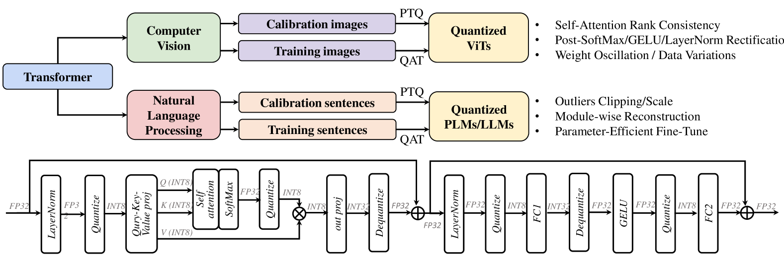
where $s_{w},s_{e},z_{e}$ are quantization parameters of weights and input embedding, and $e_{int}$ and $\textrm{w}_{int}$ are the integer input and weights, which are calculated by Equation 4. $C$ could be pre-computed with $s_{e},z_{e},s_{e}$ and $\textrm{w}_{int}$ . Thus the floating-point multiplication could be accelerated with efficient integer multiplication in the inference. To minimize the performance degradation of quantized models, different optimization methods have been proposed and they can be divided into two categories: (1) Post-training quantization (PTQ) [21, 41, 22, 42, 43, 44, 45] , mainly focuses on optimizing the quantization parameters of weights and activations with a few unlabeled calibration data, and some of the latest methods also explore adaptive rounding for weight quantization. (2) Quantization-aware training (QAT) [46, 47, 48, 49, 50, 51, 23, 52, 53, 54, 55, 56], inserts the quantization nodes into networks and conducts training with complete training data, where all the weights and quantization parameters are optimized together. In this section, we systematically introduce the research of model quantization on Transformer-based vision models and large language models, as shown in Figure 2.
<details>
<summary>x2.png Details</summary>
### Visual Description
## Diagram: Transformer Quantization Workflow for Computer Vision and NLP
### Overview
This diagram illustrates a generalized workflow for applying quantization techniques to Transformer models in both Computer Vision (CV) and Natural Language Processing (NLP) domains. It shows how different types of input data (images and sentences) are processed through a Transformer architecture, leading to quantized models. The diagram also depicts two distinct, detailed sub-workflows representing the internal processing of a quantized Transformer block, likely for either CV or NLP tasks, showing the flow of data through various operations like normalization, quantization, attention mechanisms, and feed-forward layers.
### Components/Axes
The diagram is structured into three main sections:
**Top Section: High-Level Workflow**
* **Input Branches:**
* **Transformer (Blue Box):** A central component from which two main processing branches originate.
* **Computer Vision (Green Box):** Represents the application domain for image data.
* **Natural Language Processing (Pink Box):** Represents the application domain for text data.
* **Data Types:**
* **Calibration images (Purple Box):** Input data for CV calibration.
* **Training images (Purple Box):** Input data for CV training.
* **Calibration sentences (Orange Box):** Input data for NLP calibration.
* **Training sentences (Orange Box):** Input data for NLP training.
* **Quantization Methods:**
* **PTQ (Post-Training Quantization):** A label indicating a quantization method applied to calibration data.
* **QAT (Quantization-Aware Training):** A label indicating a quantization method applied to training data.
* **Output Models:**
* **Quantized ViTs (Yellow Box):** Represents quantized Vision Transformers.
* **Quantized PLMs/LLMs (Yellow Box):** Represents quantized Pre-trained Language Models / Large Language Models.
* **Associated Techniques/Challenges:**
* **For Quantized ViTs:**
* Self-Attention Rank Consistency
* Post-SoftMax/GELU/LayerNorm Rectification
* Weight Oscillation / Data Variations
* **For Quantized PLMs/LLMs:**
* Outliers Clipping/Scale
* Module-wise Reconstruction
* Parameter-Efficient Fine-Tune
**Bottom Section: Detailed Quantized Transformer Block (Left)**
This section depicts a detailed view of a Transformer block, likely for processing input features.
* **Input Data Type:**
* **FP32:** Indicates input data is in 32-bit floating-point format.
* **Sequential Operations (Rectangular Boxes):**
* **LayerNorm:** Layer Normalization.
* **Quantize:** Quantization operation.
* **Q (INT8), K (INT8), V (INT8):** Query, Key, and Value projections, with data quantized to 8-bit integers.
* **Self attention:** Self-attention mechanism.
* **SoftMax:** Softmax activation function.
* **FP32:** Intermediate output in 32-bit floating-point format.
* **Quantize:** Another quantization operation.
* **out proj:** Output projection.
* **INT8:** Output data quantized to 8-bit integers.
* **INT32:** Intermediate data in 32-bit integers.
* **Dequantize:** Dequantization operation.
* **FP32:** Output data in 32-bit floating-point format.
* **Operations (Symbols):**
* **⊕ (Circle with Plus):** Element-wise addition (residual connection).
**Bottom Section: Detailed Quantized Transformer Block (Right)**
This section depicts another detailed view of a Transformer block, likely a subsequent layer or a different type of block.
* **Input Data Type:**
* **FP32:** Indicates input data is in 32-bit floating-point format.
* **Sequential Operations (Rectangular Boxes):**
* **LayerNorm:** Layer Normalization.
* **Quantize:** Quantization operation.
* **INT8:** Output data quantized to 8-bit integers.
* **FC1:** First Feed-Forward layer (likely a linear transformation).
* **INT32:** Intermediate data in 32-bit integers.
* **Dequantize:** Dequantization operation.
* **FP32:** Output data in 32-bit floating-point format.
* **GELU:** Gaussian Error Linear Unit activation function.
* **Quantize:** Another quantization operation.
* **INT8:** Output data quantized to 8-bit integers.
* **FC2:** Second Feed-Forward layer (likely a linear transformation).
* **FP32:** Output data in 32-bit floating-point format.
* **Operations (Symbols):**
* **⊕ (Circle with Plus):** Element-wise addition (residual connection).
* **Loop Arrow:** Indicates a residual connection from a previous layer (or the input) to the output of the FC2 layer before the final addition.
### Detailed Analysis or Content Details
**Top Section:**
* The diagram shows that a "Transformer" architecture can be applied to both "Computer Vision" and "Natural Language Processing".
* For CV, "Calibration images" are processed via "PTQ" to yield "Quantized ViTs". "Training images" are processed via "QAT" to yield "Quantized ViTs".
* For NLP, "Calibration sentences" are processed via "PTQ" to yield "Quantized PLMs/LLMs". "Training sentences" are processed via "QAT" to yield "Quantized PLMs/LLMs".
* The associated bullet points for "Quantized ViTs" highlight potential issues like "Self-Attention Rank Consistency", "Post-SoftMax/GELU/LayerNorm Rectification", and "Weight Oscillation / Data Variations".
* The associated bullet points for "Quantized PLMs/LLMs" highlight potential issues like "Outliers Clipping/Scale", "Module-wise Reconstruction", and "Parameter-Efficient Fine-Tune".
**Bottom Section (Left Block):**
* The flow starts with **FP32** data.
* It passes through **LayerNorm**, then is **Quantized**. The diagram indicates a transition to INT8 for Q, K, V.
* This is followed by a projection into **Query (INT8)**, **Key (INT8)**, and **Value (INT8)**.
* These are fed into a **Self attention** mechanism, followed by **SoftMax**.
* The output of SoftMax is **FP32**.
* This FP32 output is then **Quantized** to **INT8**.
* This INT8 output is then processed by an **out proj** layer, resulting in **INT8** data.
* This INT8 data is then converted to **INT32** and subsequently **Dequantized** back to **FP32**.
* Finally, this FP32 output is added element-wise (residual connection) with another FP32 input (indicated by the ⊕ symbol).
**Bottom Section (Right Block):**
* The flow starts with **FP32** data.
* It passes through **LayerNorm**, then is **Quantized** to **INT8**.
* This INT8 data is processed by **FC1**, resulting in **INT32** data.
* This INT32 data is then **Dequantized** to **FP32**.
* This FP32 data passes through a **GELU** activation.
* The output of GELU is then **Quantized** to **INT8**.
* This INT8 data is processed by **FC2**, resulting in **FP32** data.
* Finally, this FP32 output is added element-wise (residual connection) with another FP32 input (indicated by the ⊕ symbol). A loop arrow indicates this residual connection originates from a point earlier in the network, likely before the LayerNorm in this block.
### Key Observations
* The diagram clearly distinguishes between Post-Training Quantization (PTQ) and Quantization-Aware Training (QAT), with PTQ using calibration data and QAT using training data.
* Both CV (ViTs) and NLP (PLMs/LLMs) models are shown to undergo similar quantization workflows.
* The detailed sub-diagrams illustrate a common pattern in Transformer blocks: normalization, quantization, attention/projection, activation, and residual connections.
* There's a significant amount of quantization and dequantization happening within the detailed blocks, suggesting a focus on mixed-precision or aggressive quantization.
* The presence of INT8 and INT32 data types indicates the use of low-precision integer representations for computational efficiency.
* The residual connections (⊕) are crucial for maintaining model performance during quantization, a standard practice in deep learning architectures.
* The specific challenges listed for ViTs and PLMs/LLMs suggest areas of active research and potential pitfalls in quantizing these models.
### Interpretation
This diagram outlines a generalized methodology for quantizing Transformer models for both computer vision and natural language processing tasks. It highlights that the choice of quantization method (PTQ vs. QAT) depends on the availability of calibration or training data, respectively. The subsequent detailed sub-diagrams provide a glimpse into the internal mechanics of how these quantized models operate, showcasing the interplay between various operations like normalization, attention, feed-forward layers, and crucially, the repeated quantization and dequantization steps.
The diagram suggests that achieving effective quantization for advanced models like Vision Transformers (ViTs) and Large Language Models (LLMs) involves addressing specific challenges. For ViTs, maintaining the integrity of the self-attention mechanism and mitigating issues like weight oscillation are key. For NLP models, handling outliers and employing module-wise reconstruction are important considerations. The emphasis on mixed precision (e.g., INT8, INT32, FP32) within the detailed blocks implies a strategy to balance computational efficiency with model accuracy. The residual connections are a fundamental architectural element that helps preserve information flow and gradients, which is particularly vital when reducing precision. Overall, the diagram serves as a conceptual blueprint for understanding the process and complexities of deploying quantized Transformer models in real-world applications.
</details>
Figure 2: The overview of quantization for Transformers. The top demonstrates the different problems that are addressed in existing works for computer vision and natural language processing, and the bottom shows a normal INT8 inference process of a standard Transformer block.
TABLE II: Comparison of different PTQ and QAT methods for transformer-based vision models. W/A denotes the bit-width of weight and activation and the results show the top-1 accuracy on ImageNet-1k validation set. * represents for mixed-precision.
| Method of PTQ | W/A (bit) | ViT-B | DeiT-S | DeiT-B | Swin-S | Swin-B |
| --- | --- | --- | --- | --- | --- | --- |
| Full Precision | 32/32 | 84.54 | 79.85 | 81.80 | 83.23 | 85.27 |
| PTQ-ViT [21] | 8*/8* | 76.98 | 78.09 | 81.29 | - | - |
| PTQ4ViT [41] | 8/8 | 84.54 | 79.47 | 81.48 | 83.10 | 85.14 |
| FQ-ViT [22] | 8/8 | 83.31 | 79.17 | 81.20 | 82.71 | 82.97 |
| APQ-ViT [42] | 8/8 | 84.26 | 79.78 | 81.72 | 83.16 | 85.16 |
| NoiseQuant [44] | 8/8 | 84.22 | 79.51 | 81.45 | 83.13 | 85.20 |
| PTQ-ViT [21] | 6*/6* | 75.26 | 75.10 | 77.47 | - | - |
| PTQ4ViT [41] | 6/6 | 81.65 | 76.28 | 80.25 | 82.38 | 84.01 |
| APQ-ViT [42] | 6/6 | 82.21 | 77.76 | 80.42 | 84.18 | 85.60 |
| NoiseQuant [44] | 6/6 | 82.32 | 77.43 | 80.70 | 82.86 | 84.68 |
| RepQ-ViT [45] | 6/6 | 83.62 | 78.90 | 81.27 | 82.79 | 84.57 |
| APQ-ViT [42] | 4/8 | 72.63 | 77.14 | 79.55 | 80.56 | 81.94 |
| PTQ-ViT [21] | 4*/4* | - | - | 75.94 | - | - |
| APQ-ViT [42] | 4/4 | 41.41 | 43.55 | 67.48 | 83.16 | 85.16 |
| RepQ-ViT [45] | 4/4 | 68.48 | 69.03 | 75.61 | 79.45 | 78.32 |
| Method of QAT | W/A (bit) | DeiT-T | DeiT-S | DeiT-B | Swin-T | Swin-S |
| Full Precision | 32/32 | 72.20 | 79.85 | 81.80 | 81.20 | 83.23 |
| I-ViT [50] | 8/8 | 72.24 | 80.12 | 81.74 | 81.50 | 83.01 |
| Q-ViT [48] | 4/4 | 72.79 | 80.11 | - | 80.59 | - |
| AFQ-ViT [48] | 4/4 | - | 80.90 | 83.00 | 82.50 | 84.40 |
| Quantformer [46] | 4/4 | 69.90 | 78.20 | 79.70 | 78.30 | 81.00 |
| OFQ [23] | 4/4 | 75.46 | 81.10 | - | 81.88 | - |
| VVTQ [56] | 4/4 | 74.71 | - | - | 82.42 | - |
| Q-ViT [48] | 3/3 | 69.62 | 78.08 | - | 79.45 | - |
| AFQ-ViT [48] | 3/3 | - | 79.00 | 81.00 | 80.90 | 82.70 |
| Quantformer [46] | 3/3 | 65.20 | 75.40 | 78.30 | 77.40 | 79.20 |
| OFQ [23] | 3/3 | 72.72 | 79.57 | - | 81.09 | - |
| AFQ-ViT [48] | 2/2 | - | 72.10 | 74.20 | 74.70 | 76.90 |
| Quantformer [46] | 2/2 | 60.70 | 65.20 | 73.80 | 74.20 | 76.60 |
| OFQ [23] | 2/2 | 64.33 | 75.72 | - | 78.52 | - |
(a) ViT-B_16
(b) ViT-B_16-224
(c) ViT-L_16
(d) ViT-L_16-224
(e) OPT-13B
(f) OPT-30B
(g) OPT-66B
<details>
<summary>x3.png Details</summary>
### Visual Description
## Bar Chart: Latency vs. Batch Size for FP16 and INT8
### Overview
This bar chart displays the latency in milliseconds (ms) for two different data types, FP16 and INT8, across various batch sizes. The x-axis represents the batch size, and the y-axis represents the latency. For each batch size, there are two bars: one for FP16 (light gray) and one for INT8 (dark red).
### Components/Axes
* **Y-axis Title**: "Latency(ms)"
* **Scale**: Linear, ranging from 0.0 to 50.0.
* **Tick Marks**: 0.0, 12.5, 25.0, 37.5, 50.0.
* **X-axis Title**: "Batch Size"
* **Categories**: 1, 8, 16, 32.
* **Legend**: Located in the top-left quadrant of the chart.
* **FP16**: Represented by a light gray rectangle.
* **INT8**: Represented by a dark red rectangle.
### Detailed Analysis
The chart presents latency values for batch sizes of 1, 8, 16, and 32.
**Batch Size 1:**
* **FP16**: The light gray bar reaches a height of approximately 2.24 ms.
* **INT8**: The dark red bar reaches a height of approximately 2.26 ms.
**Batch Size 8:**
* **FP16**: The light gray bar reaches a height of approximately 11.14 ms.
* **INT8**: The dark red bar reaches a height of approximately 7.93 ms.
**Batch Size 16:**
* **FP16**: The light gray bar reaches a height of approximately 21.5 ms.
* **INT8**: The dark red bar reaches a height of approximately 14.66 ms.
**Batch Size 32:**
* **FP16**: The light gray bar reaches a height of approximately 43.81 ms.
* **INT8**: The dark red bar reaches a height of approximately 29.07 ms.
### Key Observations
* **General Trend**: For both FP16 and INT8, latency generally increases as the batch size increases.
* **FP16 Trend**: The latency for FP16 shows a significant upward trend, with a substantial jump from batch size 16 to 32.
* **INT8 Trend**: The latency for INT8 also increases with batch size, but at a less dramatic rate compared to FP16, especially at larger batch sizes.
* **Comparison**: At batch size 1, the latencies are very similar. However, as batch size increases, FP16 consistently shows higher latency than INT8, with the difference becoming more pronounced at batch sizes 16 and 32.
### Interpretation
This chart demonstrates the impact of batch size on latency for different data precisions (FP16 and INT8). The data suggests that while increasing batch size generally leads to higher latency for both precisions, INT8 exhibits better scalability and lower latency at larger batch sizes compared to FP16. This implies that for applications where latency is a critical factor and large batch sizes are utilized, INT8 might be a more performant choice. The significant increase in latency for FP16 at batch size 32 could indicate a bottleneck or a point where the computational overhead of FP16 becomes more dominant.
</details>
<details>
<summary>x4.png Details</summary>
### Visual Description
## Bar Chart: Latency vs. Batch Size for FP16 and INT8
### Overview
This image is a bar chart that visualizes the latency (in milliseconds) for two different data types, FP16 and INT8, across varying batch sizes. The chart shows how latency changes as the batch size increases from 1 to 32.
### Components/Axes
* **Y-axis Title**: "Latency(ms)"
* **Scale**: Linear, ranging from 0.0 to 10.0, with major tick marks at 0.0, 2.5, 5.0, 7.5, and 10.0.
* **X-axis Title**: "Batch Size"
* **Categories**: The x-axis displays discrete batch sizes: 1, 8, 16, and 32.
* **Legend**: Located in the top-left quadrant of the chart.
* **FP16**: Represented by a light gray rectangle.
* **INT8**: Represented by a dark red rectangle.
### Detailed Analysis
The chart displays paired bars for each batch size, with the light gray bar representing FP16 latency and the dark red bar representing INT8 latency.
**Batch Size 1:**
* FP16 (light gray bar): 1.53 ms
* INT8 (dark red bar): 1.52 ms
**Batch Size 8:**
* FP16 (light gray bar): 3.03 ms
* INT8 (dark red bar): 2.38 ms
**Batch Size 16:**
* FP16 (light gray bar): 5.3 ms
* INT8 (dark red bar): 3.74 ms
**Batch Size 32:**
* FP16 (light gray bar): 10.04 ms
* INT8 (dark red bar): 6.43 ms
### Key Observations
* **General Trend**: For both FP16 and INT8, latency generally increases as the batch size increases.
* **FP16 Trend**: The latency for FP16 shows a significant upward trend, particularly between batch sizes 16 and 32.
* **INT8 Trend**: The latency for INT8 also increases with batch size, but at a slower rate compared to FP16, especially at larger batch sizes.
* **Comparison**: At batch size 1, the latencies for FP16 and INT8 are very close. However, as the batch size increases, INT8 consistently shows lower latency than FP16. The difference in latency becomes more pronounced at larger batch sizes (16 and 32).
### Interpretation
This bar chart demonstrates the performance characteristics of FP16 and INT8 data types in terms of latency under varying computational loads (batch sizes).
* **Data Suggests**: The data suggests that INT8 is generally more efficient in terms of latency than FP16, especially as the batch size grows. This is likely due to the reduced precision of INT8 requiring less computational resources and memory bandwidth.
* **Relationship**: The x-axis (Batch Size) is the independent variable, and the y-axis (Latency) is the dependent variable. The legend differentiates the two data types (FP16 and INT8) whose latencies are being measured.
* **Notable Trends/Anomalies**:
* The most striking trend is the superior performance of INT8 at larger batch sizes. While FP16 latency nearly doubles from batch size 16 to 32 (from 5.3 ms to 10.04 ms), INT8 latency increases by a smaller margin (from 3.74 ms to 6.43 ms).
* At batch size 1, the latencies are almost identical, indicating that for very small workloads, the overhead of data type conversion or other factors might dominate, making the precision difference less impactful.
* The steep increase in FP16 latency at larger batch sizes could indicate memory bandwidth limitations or increased computational complexity that scales poorly with batch size for higher precision data. Conversely, INT8 appears to scale more favorably.
In essence, the chart highlights a common trade-off in deep learning and other computational tasks: using lower precision data types like INT8 can lead to significant performance gains (lower latency) with a potentially acceptable loss in accuracy, especially for inference tasks. FP16, while offering higher precision, incurs a higher latency cost as the workload increases.
</details>
<details>
<summary>x5.png Details</summary>
### Visual Description
## Bar Chart: Latency vs. Batch Size for FP16 and INT8
### Overview
This image displays a bar chart comparing the latency (in milliseconds) for two different data types, FP16 and INT8, across varying batch sizes. The batch sizes tested are 1, 8, 16, and 32.
### Components/Axes
* **Y-axis Title**: "Latency(ms)"
* **Scale**: Linear, ranging from 0.0 to 130.0. Major tick marks are at 0.0, 32.5, 65.0, 97.5, and 130.0.
* **X-axis Title**: "Batch Size"
* **Categories**: 1, 8, 16, 32.
* **Legend**: Located in the top-left quadrant of the chart.
* **FP16**: Represented by a light gray rectangle.
* **INT8**: Represented by a dark red rectangle.
### Detailed Analysis or Content Details
The chart presents data for four different batch sizes, with two bars for each batch size representing FP16 and INT8.
**Batch Size 1:**
* **FP16**: The light gray bar reaches a height of approximately 5.36 ms.
* **INT8**: The dark red bar reaches a height of approximately 4.77 ms.
**Batch Size 8:**
* **FP16**: The light gray bar reaches a height of approximately 30.95 ms.
* **INT8**: The dark red bar reaches a height of approximately 20.25 ms.
**Batch Size 16:**
* **FP16**: The light gray bar reaches a height of approximately 60.99 ms.
* **INT8**: The dark red bar reaches a height of approximately 39.43 ms.
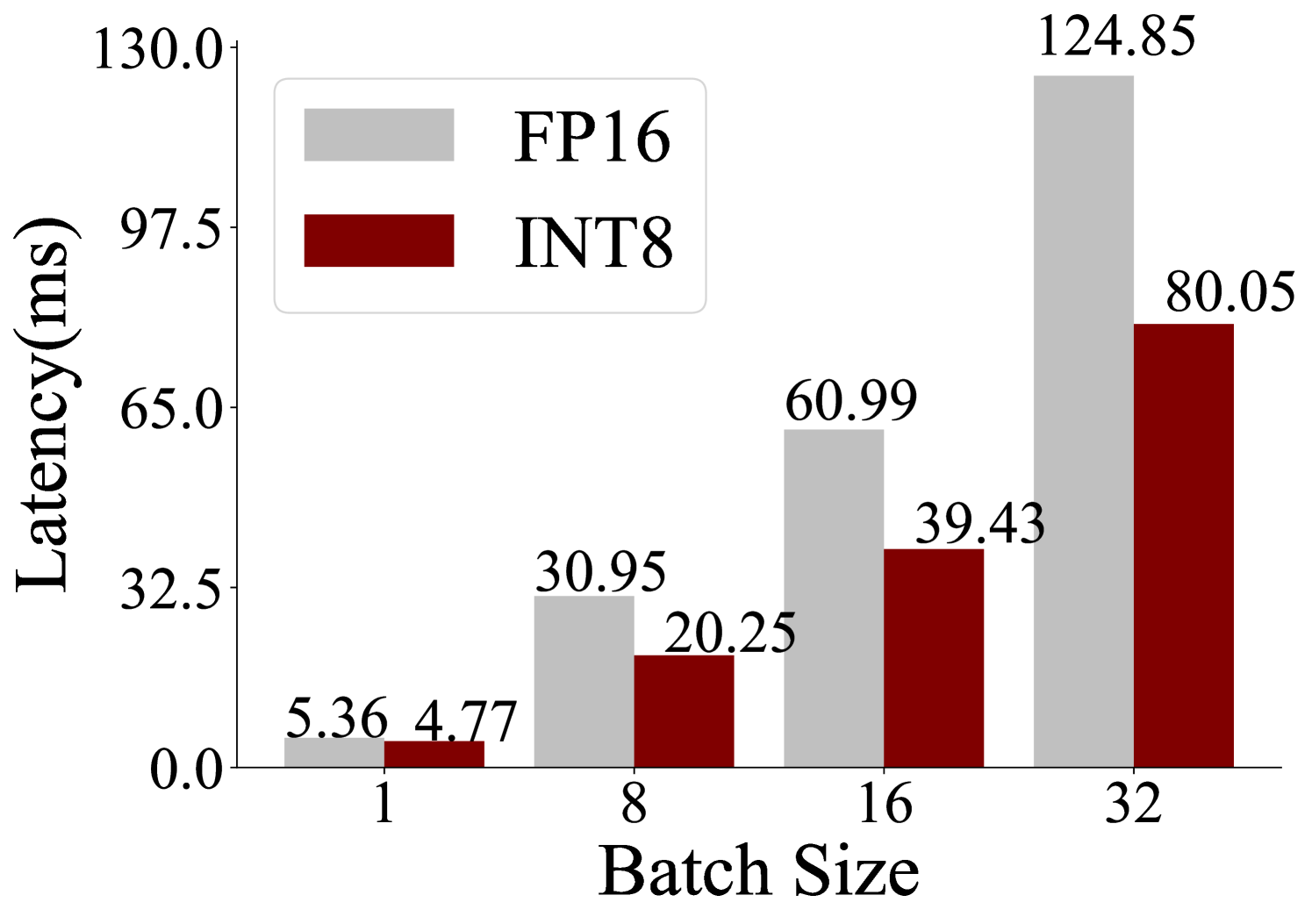
**Batch Size 32:**
* **FP16**: The light gray bar reaches a height of approximately 124.85 ms.
* **INT8**: The dark red bar reaches a height of approximately 80.05 ms.
### Key Observations
* **Trend**: For both FP16 and INT8, latency generally increases as the batch size increases.
* **Comparison**: Across all batch sizes, FP16 consistently exhibits higher latency than INT8.
* **Rate of Increase**: The latency increase appears to be more pronounced for FP16, especially between batch sizes 16 and 32.
### Interpretation
This bar chart demonstrates the performance characteristics of FP16 and INT8 data types in terms of latency as batch size varies. The data suggests that INT8 is a more efficient data type, resulting in lower latency compared to FP16, particularly at larger batch sizes. This is likely due to the reduced precision of INT8 requiring less computational resources and memory bandwidth. The increasing latency with batch size is a common phenomenon, indicating that processing larger batches takes more time. The significant jump in latency for FP16 at batch size 32 might suggest a performance bottleneck or saturation point for this data type under high load. This information is crucial for optimizing deep learning model inference or training, where choosing the appropriate data type and batch size can significantly impact performance and throughput.
</details>
<details>
<summary>x6.png Details</summary>
### Visual Description
## Bar Chart: Latency vs. Batch Size for FP16 and INT8
### Overview
This image is a bar chart comparing the latency (in milliseconds) for two different data types, FP16 and INT8, across various batch sizes. The chart displays four sets of paired bars, each representing a specific batch size: 1, 8, 16, and 32.
### Components/Axes
* **Y-axis Title**: "Latency(ms)"
* **Scale**: Linear, ranging from 0.0 to 30.0, with major tick marks at 0.0, 7.5, 15.0, 22.5, and 30.0.
* **X-axis Title**: "Batch Size"
* **Categories**: 1, 8, 16, 32.
* **Legend**: Located in the top-left quadrant of the chart.
* **FP16**: Represented by a light gray rectangle.
* **INT8**: Represented by a dark maroon rectangle.
### Detailed Analysis
The chart presents latency values for FP16 and INT8 at batch sizes of 1, 8, 16, and 32.
**Batch Size 1:**
* **FP16**: The light gray bar reaches a height of approximately 2.97 ms.
* **INT8**: The dark maroon bar reaches a height of approximately 2.91 ms.
**Batch Size 8:**
* **FP16**: The light gray bar reaches a height of approximately 8.09 ms.
* **INT8**: The dark maroon bar reaches a height of approximately 5.44 ms.
**Batch Size 16:**
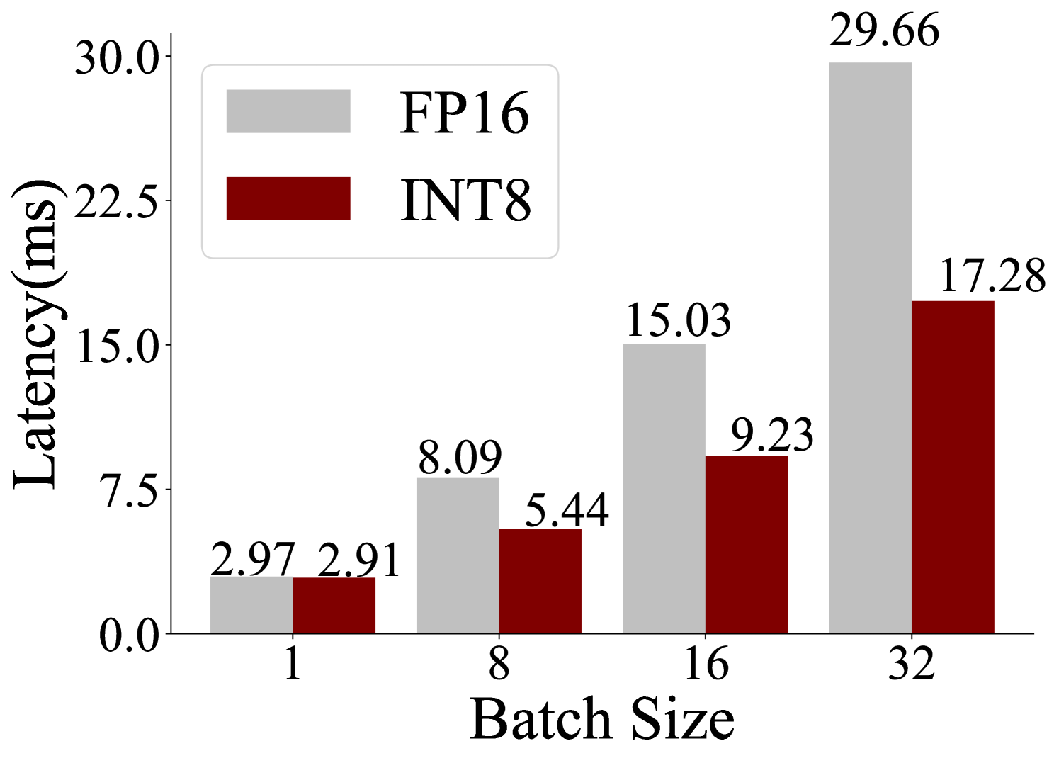
* **FP16**: The light gray bar reaches a height of approximately 15.03 ms.
* **INT8**: The dark maroon bar reaches a height of approximately 9.23 ms.
**Batch Size 32:**
* **FP16**: The light gray bar reaches a height of approximately 29.66 ms.
* **INT8**: The dark maroon bar reaches a height of approximately 17.28 ms.
### Key Observations
* **General Trend**: For both FP16 and INT8, latency generally increases as the batch size increases.
* **FP16 Trend**: The latency for FP16 shows a significant upward trend, accelerating with larger batch sizes.
* **INT8 Trend**: The latency for INT8 also increases with batch size, but at a slower rate compared to FP16, especially at larger batch sizes.
* **Comparison**: At batch size 1, FP16 and INT8 have very similar latencies. However, as batch size increases, FP16 consistently exhibits higher latency than INT8. The difference in latency between FP16 and INT8 becomes more pronounced at batch sizes 16 and 32.
### Interpretation
This chart demonstrates the performance characteristics of FP16 and INT8 data types in terms of latency as batch size varies. The data suggests that while both data types experience increased latency with larger batch sizes, INT8 offers a more favorable latency profile, particularly for larger batch sizes. This implies that INT8 might be a more efficient choice for applications requiring high throughput and low latency when dealing with substantial amounts of data. The increasing divergence in latency between FP16 and INT8 as batch size grows could be attributed to factors like memory bandwidth, computational efficiency, or specific hardware optimizations for integer operations. The initial similarity at batch size 1 might indicate that overheads dominate at very small batch sizes, masking the underlying performance differences.
</details>
<details>
<summary>x7.png Details</summary>
### Visual Description
## Bar Chart: Latency vs. Batch Size for FP16 and w8a8
### Overview
This image is a bar chart that compares the latency (in milliseconds) for two different configurations, FP16 and w8a8, across varying batch sizes. The batch sizes tested are 128, 256, 512, and 1024.
### Components/Axes
* **Y-axis Title**: "Latency(ms)"
* **Scale**: Ranges from 0 to 200, with major tick marks at 0, 50, 100, 150, and 200.
* **X-axis Title**: "Batch Size"
* **Categories**: 128, 256, 512, 1024.
* **Legend**: Located in the top-left quadrant of the chart.
* **FP16**: Represented by a light gray rectangle.
* **w8a8**: Represented by a dark red rectangle.
### Detailed Analysis
The chart displays paired bars for each batch size, with the left bar representing FP16 and the right bar representing w8a8.
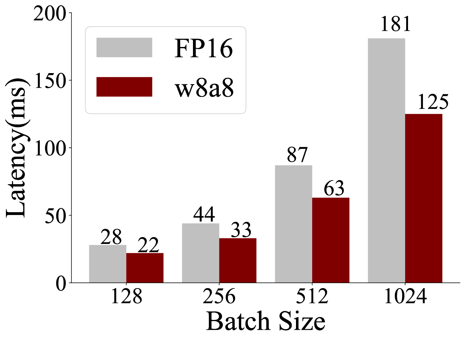
* **Batch Size 128**:
* FP16 (light gray bar): 28 ms
* w8a8 (dark red bar): 22 ms
* **Trend**: For this batch size, w8a8 has lower latency than FP16.
* **Batch Size 256**:
* FP16 (light gray bar): 44 ms
* w8a8 (dark red bar): 33 ms
* **Trend**: For this batch size, w8a8 has lower latency than FP16.
* **Batch Size 512**:
* FP16 (light gray bar): 87 ms
* w8a8 (dark red bar): 63 ms
* **Trend**: For this batch size, w8a8 has lower latency than FP16.
* **Batch Size 1024**:
* FP16 (light gray bar): 181 ms
* w8a8 (dark red bar): 125 ms
* **Trend**: For this batch size, w8a8 has lower latency than FP16.
**Overall Trend for both FP16 and w8a8**: As the batch size increases, the latency for both configurations increases significantly. The FP16 configuration consistently shows higher latency than the w8a8 configuration across all tested batch sizes.
### Key Observations
* The latency for both FP16 and w8a8 increases with increasing batch size.
* The w8a8 configuration consistently exhibits lower latency compared to the FP16 configuration for all batch sizes.
* The difference in latency between FP16 and w8a8 appears to widen as the batch size increases.
### Interpretation
This bar chart demonstrates the performance characteristics of two different configurations (FP16 and w8a8) in terms of latency as a function of batch size. The data suggests that the w8a8 configuration is more efficient, offering lower latency across all tested batch sizes. This could be due to optimizations or a more suitable data representation for the underlying hardware or software being used. The increasing latency with larger batch sizes is a common observation in many computational systems, often related to memory constraints, processing overhead, or communication bottlenecks. The widening gap in latency at larger batch sizes might indicate that FP16 scales less favorably than w8a8 under higher load. This information is crucial for system designers and engineers when choosing configurations for optimal performance, especially in scenarios where low latency is a critical requirement.
</details>
<details>
<summary>x8.png Details</summary>
### Visual Description
## Bar Chart: Latency vs. Batch Size for FP16 and w8a8
### Overview
This bar chart displays the latency in milliseconds (ms) for two different configurations, FP16 and w8a8, across varying batch sizes. The batch sizes tested are 128, 256, 512, and 1024. The chart visually represents how latency changes with increasing batch sizes for each configuration.
### Components/Axes
* **Y-axis Title:** "Latency(ms)"
* **Scale:** Linear, ranging from 0 to 400, with major tick marks at 0, 100, 200, 300, and 400.
* **X-axis Title:** "Batch Size"
* **Categories:** 128, 256, 512, 1024.
* **Legend:** Located in the top-left quadrant of the chart.
* **FP16:** Represented by a light gray rectangle.
* **w8a8:** Represented by a dark red rectangle.
### Detailed Analysis
The chart presents paired bars for each batch size, with the left bar representing FP16 and the right bar representing w8a8.
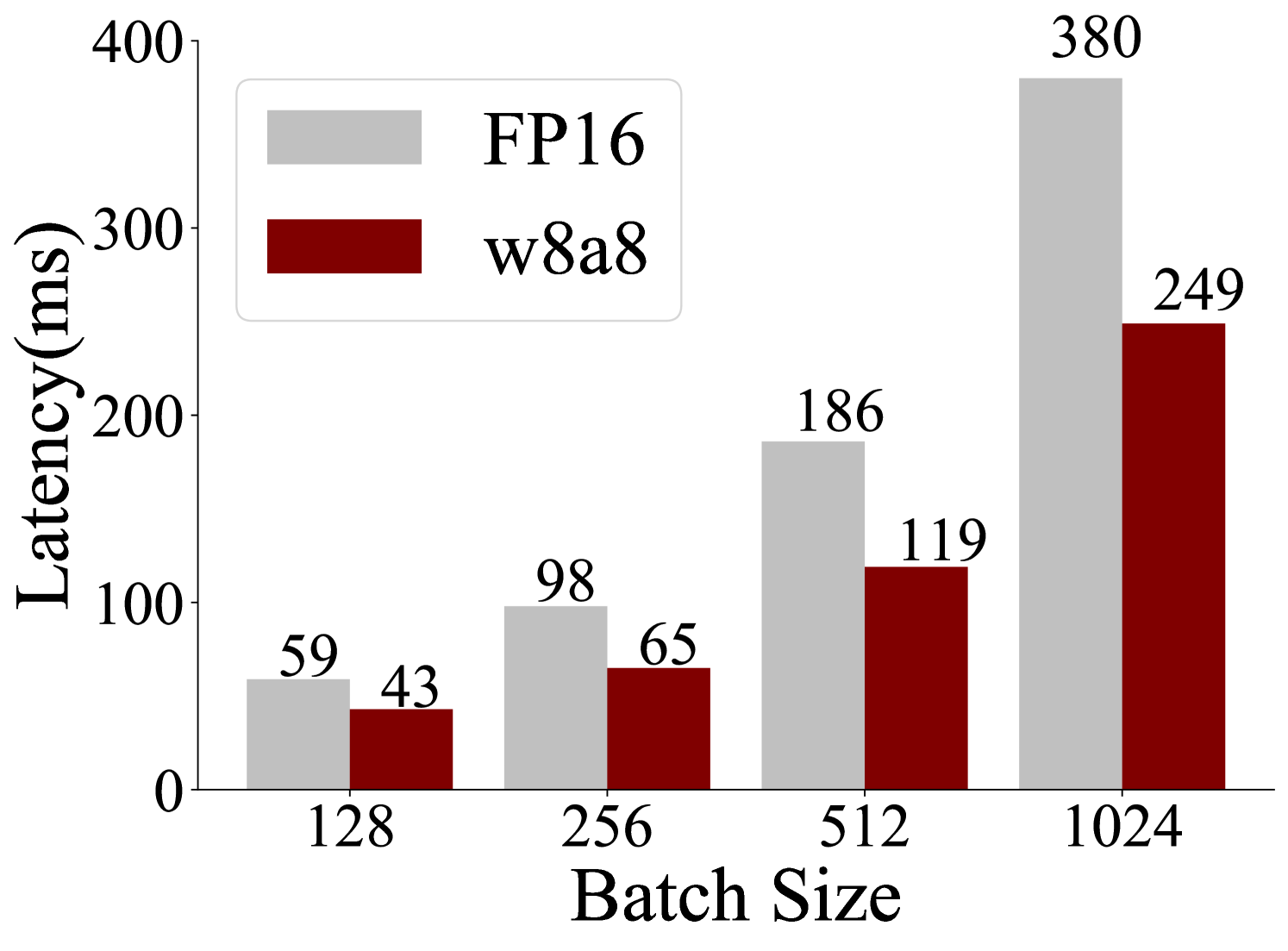
* **Batch Size 128:**
* FP16 (light gray bar): 59 ms. This bar is positioned to the left of the w8a8 bar.
* w8a8 (dark red bar): 43 ms. This bar is positioned to the right of the FP16 bar.
* **Batch Size 256:**
* FP16 (light gray bar): 98 ms. This bar is positioned to the left of the w8a8 bar.
* w8a8 (dark red bar): 65 ms. This bar is positioned to the right of the FP16 bar.
* **Batch Size 512:**
* FP16 (light gray bar): 186 ms. This bar is positioned to the left of the w8a8 bar.
* w8a8 (dark red bar): 119 ms. This bar is positioned to the right of the FP16 bar.
* **Batch Size 1024:**
* FP16 (light gray bar): 380 ms. This bar is positioned to the left of the w8a8 bar.
* w8a8 (dark red bar): 249 ms. This bar is positioned to the right of the FP16 bar.
### Key Observations
* **Trend:** For both FP16 and w8a8, latency generally increases as the batch size increases.
* **Comparison:** The w8a8 configuration consistently shows lower latency than the FP16 configuration across all tested batch sizes.
* **Magnitude of Difference:** The difference in latency between FP16 and w8a8 appears to grow with increasing batch size. For batch size 128, the difference is approximately 16 ms (59 - 43). For batch size 1024, the difference is approximately 131 ms (380 - 249).
* **Steepest Increase:** The most significant jump in latency for FP16 occurs between batch sizes 512 (186 ms) and 1024 (380 ms), an increase of 194 ms. For w8a8, the largest increase is between batch sizes 512 (119 ms) and 1024 (249 ms), an increase of 130 ms.
### Interpretation
This chart demonstrates the performance characteristics of two different data precision/quantization schemes (FP16 and w8a8) in terms of latency as a function of batch size.
The data suggests that the w8a8 configuration is more efficient, exhibiting lower latency across all batch sizes. This is likely due to its reduced precision (8-bit weights and 8-bit activations) compared to FP16 (16-bit floating-point), which can lead to faster computations and reduced memory bandwidth requirements.
The increasing latency with larger batch sizes is a common phenomenon in many computational systems, often attributed to factors like increased memory usage, cache contention, and parallel processing overhead. The fact that the latency difference between FP16 and w8a8 widens with larger batch sizes indicates that the benefits of w8a8 become more pronounced as the workload scales up. This implies that for applications requiring high throughput and processing large amounts of data (larger batch sizes), the w8a8 configuration offers a significant performance advantage. The steep increase in latency for FP16 at batch size 1024 might indicate a saturation point or a more significant bottleneck compared to w8a8 at that scale.
</details>
<details>
<summary>x9.png Details</summary>
### Visual Description
## Bar Chart: Latency vs. Batch Size for FP16 and w8a8
### Overview
This image is a bar chart that compares the latency (in milliseconds) for two different data types, FP16 and w8a8, across various batch sizes. The chart displays four sets of paired bars, each representing a specific batch size: 128, 256, 512, and 1024. For each batch size, there are two bars: a light gray bar representing FP16 and a dark red bar representing w8a8. The height of each bar corresponds to the measured latency.
### Components/Axes
* **Y-axis Title**: "Latency(ms)"
* **Scale**: The y-axis ranges from 0 to 500, with major tick marks at 0, 125, 250, 375, and 500.
* **X-axis Title**: "Batch Size"
* **Categories**: The x-axis displays four batch sizes: 128, 256, 512, and 1024.
* **Legend**: Located in the top-left quadrant of the chart.
* **FP16**: Represented by a light gray rectangle.
* **w8a8**: Represented by a dark red rectangle.
### Detailed Analysis
The chart presents the following data points:
* **Batch Size 128**:
* FP16 (light gray bar): 79 ms
* w8a8 (dark red bar): 75 ms
* *Trend*: For batch size 128, w8a8 has a slightly lower latency than FP16.
* **Batch Size 256**:
* FP16 (light gray bar): 122 ms
* w8a8 (dark red bar): 131 ms
* *Trend*: For batch size 256, FP16 has a lower latency than w8a8.
* **Batch Size 512**:
* FP16 (light gray bar): 236 ms
* w8a8 (dark red bar): 229 ms
* *Trend*: For batch size 512, w8a8 has a slightly lower latency than FP16.
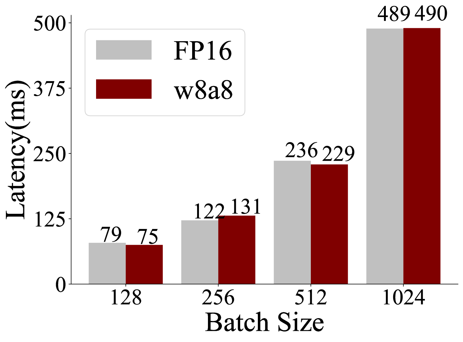
* **Batch Size 1024**:
* FP16 (light gray bar): 489 ms
* w8a8 (dark red bar): 490 ms
* *Trend*: For batch size 1024, FP16 has a slightly lower latency than w8a8.
### Key Observations
* **Overall Trend**: Latency increases significantly with increasing batch size for both FP16 and w8a8.
* **Comparison**:
* At batch sizes 128 and 512, w8a8 shows a slightly lower latency compared to FP16.
* At batch sizes 256 and 1024, FP16 shows a slightly lower latency compared to w8a8.
* **Magnitude of Difference**: The latency difference between FP16 and w8a8 is relatively small across all batch sizes, generally within a range of approximately 1-5 ms, except for batch size 256 where the difference is 9 ms.
* **Peak Latency**: The highest latencies are observed at the largest batch size (1024), with values close to 500 ms for both data types.
### Interpretation
This bar chart demonstrates the performance characteristics of FP16 and w8a8 data types in terms of latency as batch size varies. The data suggests that:
1. **Scalability**: Both FP16 and w8a8 exhibit a clear trend of increasing latency as the batch size grows. This is a common behavior in computational tasks, as larger batches require more processing power and memory, leading to longer execution times.
2. **Data Type Performance**: The comparison between FP16 and w8a8 reveals that their performance is quite similar across different batch sizes. There isn't a consistent winner; sometimes w8a8 is slightly faster, and at other times FP16 is. This suggests that for this particular task or hardware configuration, the choice between FP16 and w8a8 might not lead to a dramatic difference in latency, especially at smaller batch sizes. The slight variations could be attributed to factors like hardware optimization, memory access patterns, or specific algorithmic implementations.
3. **Batch Size Impact**: The most significant factor influencing latency is the batch size. The latency more than doubles when moving from batch size 128 to 256, and continues to increase substantially for larger batch sizes. This highlights the importance of selecting an appropriate batch size for optimal performance, balancing throughput with latency requirements.
4. **Near Equivalence at High Load**: At the highest batch size (1024), the latencies for FP16 and w8a8 are almost identical (489 ms vs. 490 ms). This could indicate that at such high loads, the system's resources are saturated, and both data types are experiencing similar bottlenecks, making their relative efficiency less distinguishable.
In essence, the chart provides empirical evidence for the latency behavior of these two data types under varying computational loads, indicating that while batch size is a dominant factor, the performance difference between FP16 and w8a8 is marginal and context-dependent.
</details>
<details>
<summary>x10.png Details</summary>
### Visual Description
## Bar Chart: Latency vs. Batch Size for FP16 and w8a8
### Overview
This bar chart displays the latency in milliseconds (ms) for two different configurations, FP16 and w8a8, across varying batch sizes. The x-axis represents the batch size, and the y-axis represents the latency. For each batch size, there are two bars: a light gray bar representing FP16 and a dark red bar representing w8a8.
### Components/Axes
* **Title:** Implicitly, the chart compares latency performance.
* **X-axis Title:** "Batch Size"
* **X-axis Markers:** 128, 256, 512, 1024
* **Y-axis Title:** "Latency(ms)"
* **Y-axis Markers:** 0, 225, 450, 675, 900
* **Legend:** Located in the top-left quadrant of the chart.
* **FP16:** Represented by a light gray rectangle.
* **w8a8:** Represented by a dark red rectangle.
### Detailed Analysis or Content Details
The chart presents data for four distinct batch sizes:
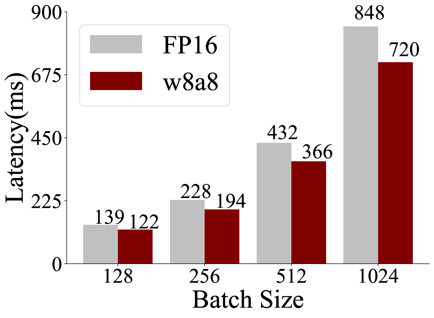
* **Batch Size 128:**
* FP16 (light gray bar): 139 ms
* w8a8 (dark red bar): 122 ms
* **Batch Size 256:**
* FP16 (light gray bar): 228 ms
* w8a8 (dark red bar): 194 ms
* **Batch Size 512:**
* FP16 (light gray bar): 432 ms
* w8a8 (dark red bar): 366 ms
* **Batch Size 1024:**
* FP16 (light gray bar): 848 ms
* w8a8 (dark red bar): 720 ms
### Key Observations
* **Trend:** For both FP16 and w8a8, latency generally increases as the batch size increases. This is visually evident as the bars grow taller with larger batch sizes.
* **Comparison:** In all tested batch sizes, the w8a8 configuration consistently exhibits lower latency compared to the FP16 configuration.
* **Magnitude of Difference:** The difference in latency between FP16 and w8a8 appears to grow with increasing batch size.
* At batch size 128, the difference is approximately 17 ms (139 - 122).
* At batch size 256, the difference is approximately 34 ms (228 - 194).
* At batch size 512, the difference is approximately 66 ms (432 - 366).
* At batch size 1024, the difference is approximately 128 ms (848 - 720).
### Interpretation
This bar chart demonstrates the performance trade-offs between two configurations, FP16 and w8a8, in terms of latency as a function of batch size. The data strongly suggests that the w8a8 configuration is more efficient, offering lower latency across all tested batch sizes. Furthermore, the performance advantage of w8a8 over FP16 becomes more pronounced at larger batch sizes. This implies that for applications requiring high throughput (larger batch sizes) and low latency, the w8a8 configuration would be the preferred choice. The increasing latency with batch size is a common characteristic in many computational tasks, as larger workloads can lead to increased processing time and resource contention. The consistent superiority of w8a8 indicates a potential optimization in its architecture or implementation that allows it to handle larger batches with less overhead.
</details>
(a) ViT-B_16
(b) ViT-B_16-224
(c) ViT-L_16
(d) ViT-L_16-224
(e) OPT-13B
(f) OPT-30B
(g) OPT-66B
(h) OPT-175B
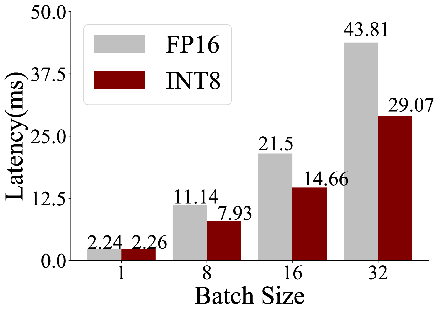
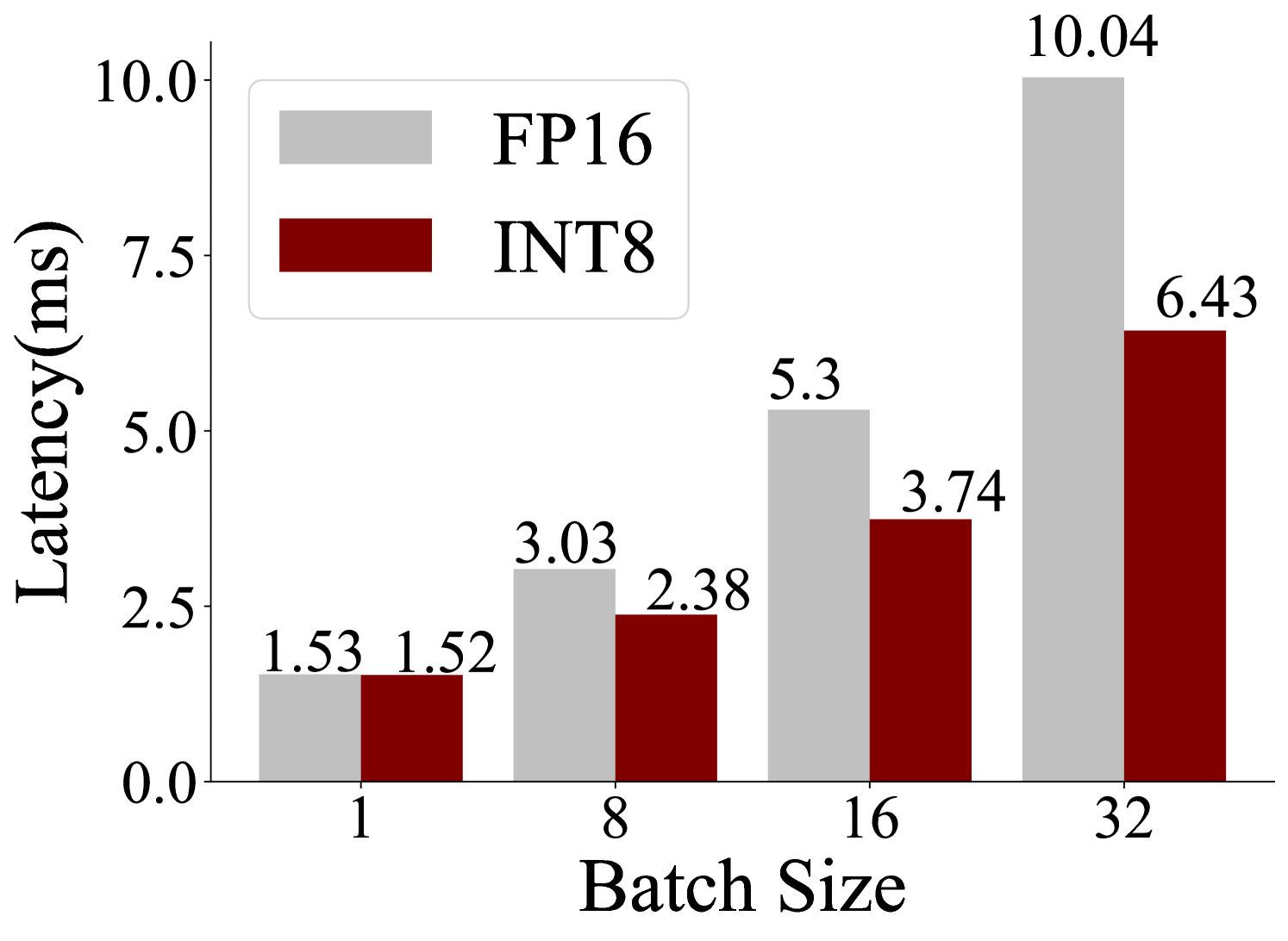
Figure 3: Inference latency of the ViT and OPT using FasterTransformer on NVIDIA A100-80GB GPUs. The data of OPT is from [18].
#### 3.1.2 Quantization for Transformer-Based Large Language Models
Before 2023, the study of quantization [57, 58, 59, 60, 61, 62, 63, 64, 65, 66] on Transformer-based NLP focused almost entirely on the BERT architecture. With the popularity of pretrained large language models [67, 1, 2], researchers [68, 69, 70] stated to explore how to quantize the Transformer with billions of parameters and explores more efficient quantization schemes with limited data and computational overhead.
Post-training quantization. Based on the analysis of outliers for quantized Transformers, Outlier Suppression [71] proposes to migrate the gamma of LayerNorm to the next module for that the gamma amplifies the outliers in the output and causes large quantization error, and then clips the tokens in a coarse-to-fine procedure. MREM [59] focuses on reducing the computational cost of quantization, and minimizes the output quantization error for all modules in parallel manner. Zeroquant [70] finds that the performance degradation is due to the different dynamic range of tokens and weights, proposes to adopt group-wise quantization for weights and token-wise quantization for activations, and utilizes knowledge distillation layer by layer. For large Transformers with billions of parameters, the outlier is still the main reason for large accuracy degradation for quantized models. To address this, LLM.int8() [68] represents the activations and outliers of weights with 16-bit and performs 8-bit vector-wise quantization for weight tensor, but the acceleration is limited and even worsened due to the irregular quantization granularity [18]. GPTQ [72] also only quantizes weight parameters as LLM.int8(), but adopts unified quantization strategy. GPTQ quantizes the weights based on approximate second-order information, thereby getting much more accurate quantized weight in a few hours. AWQ [73] proposes to search for the optimal per-channel scale factors by observing the distribution of activations instead of weights, allowing the LLMs retain the capabilities for different domains and modalities. Outlier Suppression+ [74] explores more accurate outliers suppression schemes with channel-wise shifting and scale, thereby helping align the range of different activation channels and scale down the outliers. The shifting and scale factors could also be merged with other weight parameters. Similarly, SmoothQuant [18] and QLLM [75] propose the mathematically equivalent per-channel scaling transformation that migrates the quantization difficulty from activations to weights. To further improve the performance of quantized LLMs, QLLM also learns low-rank parameters by minimizing the reconstruction error of the outputs between floating-point and quantized LLMs with limited calibration data. Similarly, RPTQ [76] utilizes a reorder-based scheme that rearranges the channels of activations with a similar range and quantizes them in cluster, and then migrates the scale into LayerNorm and weights of linear layers without extra computational overhead in the inference.Based on scale migration, OmniQuant [19] further proposes a learnable PTQ method module by module, where the weight clipping parameters and transformation scale of activations are optimized with gradient descent. To minimize error accumulation in adjacent blocks, CBQ [77] presents a cross-block reconstruction framework, simultaneously learn the rounding matrices of weight and step sizes of weights and activations. The rounding matrices are learned with LoRA technique, which does not bring much extra cost for PTQ. Like GPTQ, SqueezeLLM [78] also focuses on quantizing weights for the memory bandwidth and proposes to search for the optimal bit based on second-order information. Also, SqueezeLLM does not suppress the outliers and sensitive weight values but stores them in an efficient sparse format for more accurate quantized LLMs. Unlike the previous methods, SignRound [79] proposes to optimize quantized LLMs from the perspective of adaptive rounding. SignRound designs block-wise tuning using signed gradient descent to learn the weight rounding, thereby greatly helping the output reconstruction of each block.
TABLE III: Perplexity (PPL) comparison of different quantization methods on WikiText2. W/E denotes weights and embedding, respectively. * represents adopting different methods to get the perplexity, please refer to the corresponding papers.
| Method | PTQ | Bits | LLaMA | | | |
| --- | --- | --- | --- | --- | --- | --- |
| (W-E) | 7B | 13B | 30B | 65B | | |
| FP16 | $\times$ | 16/16 | 5.68 | 5.09 | 4.10 | 3.56 |
| SmoothQuant* [18] | ✓ | 8/8 | 11.56 | 10.08 | 7.56 | 6.20 |
| LLM-QAT* [80] | $\times$ | 8/8 | 10.30 | 9.50 | 7.10 | - |
| OS+ [74] | ✓ | 6/6 | 5.76 | 5.22 | 4.30 | 3.65 |
| OmniQuant [19] | ✓ | 6/6 | 5.96 | 5.28 | 4.38 | 3.75 |
| QLLM [75] | ✓ | 6/6 | 5.89 | 5.28 | 4.30 | 3.73 |
| SqueezeLLM [78] | ✓ | 4/16 | 5.79 | 5.18 | 4.22 | 3.76 |
| SignRound [79] | ✓ | 4/16 | 6.12 | 5.32 | 4.52 | 3.90 |
| OmniQuant [19] | ✓ | 4/16 | 5.86 | 5.21 | 4.25 | 3.71 |
| LLM-QAT* [80] | $\times$ | 4/8 | 10.90 | 10.00 | 7.50 | - |
| OS+ [74] | ✓ | 4/4- | 14.17 | 18.95 | 22.61 | 9.33 |
| OmniQuant [19] | ✓ | 4/4 | 11.26 | 10.87 | 10.33 | 9.17 |
| QLLM [75] | ✓ | 4/4 | 9.65 | 8.41 | 8.37 | 6.87 |
| PEQA [81] | $\times$ | 4/4 | 5.84 | 5.30 | 4.36 | 4.02 |
| SqueezeLLM [78] | ✓ | 3/16 | 6.32 | 5.60 | 4.66 | 4.05 |
| OmniQuant [19] | ✓ | 3/16 | 6.49 | 5.68 | 4.74 | 4.04 |
| PEQA [81] | $\times$ | 3/3 | 6.19 | 5.54 | 4.58 | 4.27 |
| OmniQuant [19] | ✓ | 2/16 | 15.47 | 13.21 | 8.71 | 7.58 |
Quantization-aware training. Q-BERT [57] is the early work that conducts quantization-aware training on Transformer-based architecture for natural language processing. Inspired by HAWQ [82], Q-BERT searches mixed-quantization settings based on the second order Hessian information and adopts group-wise quantization to partition parameter matrix into multiple groups to reduce accuracy degradation. I-BERT [62] not only quantizes the linear and self-attention layer, but also designs an integer-only inference scheme for the nonlinear operations (GELU, SoftMax and LayerNorm) in Transformers, which also inspires the FQ-ViT and I-ViT for the quantization of vision Transformer. Specifically, I-BERT proposes to use the second-order polynomial approximate for GELU and exponential function of SoftMax, and calculate the standard deviation of LayerNorm based on Newton’s Method. In this way, I-BERT can achieve faster inference compared to the baseline and normal quantization methods. To compensate for the disadvantages of the hand-crafted heuristics in Q-BERT, AQ-BERT [66] proposes an automatic mixed-precision quantization scheme to learn the bit-width and parameters of each layer simultaneously, which is inspired from differentiable network architecture search. AQ-BERT achieves better results than Q-BERT and more suitable for resource-limited devices. Besides the QAT schemes for BERT, there are only a few papers that conducts quantization-aware training on large language models for the huge training overhead. PEQA [81] and QLoRA [20] explore parameter-efficient fine-tuning techniques to train the quantized LLMs, with the former only optimizing the scale factors while freezing the quantized weights, and the latter adopting 4-bit NormalFloat, double quantization, and paged optimizers for normally distributed weights and reduce memory footprint during training. LLM-QAT [80] proposes a data-free quantization-aware training method, where the training data is generated from the original pretrained large language model. LLM-QAT not only quantizes all the linear layers and self-attention, but also quantizes the KV cache with cross-entropy based logits distillation.
#### 3.1.3 Quantization for Transformer-Based Vision Models
Post-training quantization. PTQ-ViT [21] firstly explores post-training quantization on vision Transformers, using the nuclear norm of the attention map and output feature in the Transformer layer to determine the bit-width of each layer. To get more accurate quantized Transformers, PTQ-ViT further proposes a rank loss to keep the relative order of the self-attention of quantized Transformers. PTQ4ViT [41] observers that the distributions of post-softmax and post-GELU activations are hard to quantize with conventional methods, and so introduces a twin uniform quantizer and use a Hessian guild metric to find the optimal scale parameters. To construct a full-quantized vision Transformer, FQ-ViT [22] not only quantizes all the linear and self-attention layers, but also quantizes LayerNorm and SoftMax with the power-of-two factor and Log2 quantizer. APQ-ViT [42] explores block-wise optimization scheme to determine the optimal quantizer for extremely low-bit PTQ, and utilizes an asymmetric linear quantization to quantize the attention map for maintaining the Matthew-effect of Softmax. Based on the observation that the normal uniform quantizer can not effectively handle the heavy-tailed distribution of vision Transformer activations, NoisyQuant [44] proposes to enhance the quantizer by adding a fixed uniform noise following the theoretical results, refining the quantized distribution to reduce quantization error with minimal computation cost. For the post-LayerNorm and post-SoftMax activations that have extreme distributions, RepQ-ViT [45] applies channel-wise quantization to deal with the severe inter-channel variation of the former and utilize log $\sqrt{2}$ quantizer to compress the power-law features of the later one. Before the inference, RepQ-ViT reparameterizes the scale factors to the layer-wise and log2 quantizer with mere computations.
<details>
<summary>x11.png Details</summary>
### Visual Description
## Diagram: Knowledge Distillation for Large Transformer-Based Models
### Overview
This diagram outlines the landscape of knowledge distillation techniques applied to large transformer-based models. It categorizes these techniques based on the domain (Computer Vision and Natural Language Processing) and then further subdivides them by the type of information being distilled.
### Components/Axes
The diagram is structured hierarchically:
1. **Top Level (Blue Rounded Rectangle):** "Knowledge Distillation for Large Transformer-Based Models" - This is the overarching topic.
2. **Second Level (Green and Pink Rectangles):**
* "Computer Vision" (Green)
* "Natural Language Processing" (Pink)
These represent the two primary application domains. Arrows point from the top level to these domains, indicating they are sub-categories.
3. **Third Level (Colored Rectangles with Bold Text):** These represent different distillation approaches within each domain.
* **Under Computer Vision:**
* "Logits-based" (Purple)
* "Hint-based" (Yellow)
* "Others" (Gray)
* **Under Natural Language Processing:**
* "Logits-based" (Purple)
* "Hint-based" (Yellow)
* "API-based" (Orange)
* "Others" (Gray)
Arrows point from the domain rectangles to these sub-categories.
4. **Fourth Level (Bullet Points):** These list specific examples of models or methods within each distillation approach. Each approach has a brief description of what is being distilled.
### Detailed Analysis
**Computer Vision Domain:**
* **Logits-based (Purple):**
* Description: Output logits
* Examples:
* DeiT
* TinyViT
* **Hint-based (Yellow):**
* Description: Intermediate features
* Examples:
* ViTKD
* ManifoldKD
* **Others (Gray):**
* Description: Other contexts
* Examples:
* GPT4Image
* BLIP
**Natural Language Processing Domain:**
* **Logits-based (Purple):**
* Description: Output logits
* Examples:
* DistilBERT
* MINILLM
* **Hint-based (Yellow):**
* Description: Intermediate features
* Examples:
* MobileBERT
* TinyBERT
* **API-based (Orange):**
* Description: Generated contexts
* Examples:
* PaD
* Lion
* **Others (Gray):**
* Description: Parameters
* Examples:
* Bert-of-theseus
* ProKT
### Key Observations
* The diagram clearly distinguishes between knowledge distillation for Computer Vision and Natural Language Processing.
* Both domains share "Logits-based" and "Hint-based" distillation approaches.
* Natural Language Processing has an additional category, "API-based," which is not present in Computer Vision.
* The "Others" category exists in both domains, suggesting a catch-all for methods that don't fit the primary classifications.
* Specific model names are provided as concrete examples for each category, offering a practical view of these distillation techniques.
### Interpretation
This diagram provides a structured taxonomy of knowledge distillation strategies for large transformer models. It illustrates that the core principles of distillation, such as leveraging output logits or intermediate features, are applicable across different AI domains. The divergence in NLP with the "API-based" category suggests that the nature of interaction with large language models (e.g., through APIs) can lead to unique distillation paradigms. The presence of an "Others" category in both domains highlights the evolving nature of research and the potential for novel distillation methods that may not fit neatly into existing frameworks. Overall, the diagram serves as a useful map for understanding the current approaches and potential research directions in making large transformer models more efficient through knowledge distillation.
</details>
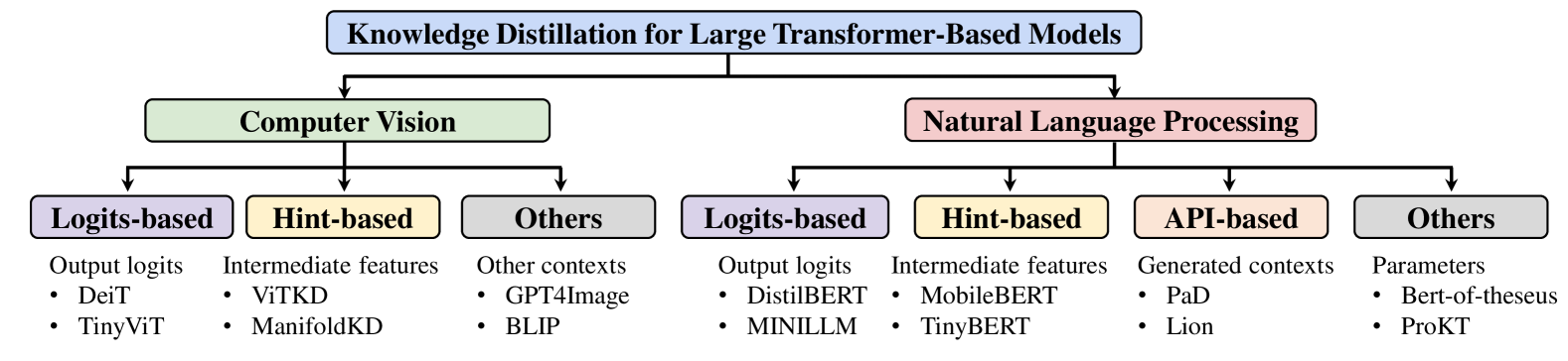
Figure 4: The taxonomy of knowledge distillation used for large Transformer-based models.
Quantization-aware training. When compressing vision Transformers to extremely low-bit precision, PTQ can not optimize the large quantization error with limited calibration images and suffers from significant performance reduction. As such, QAT is urgently required for more accurate low-bit vision Transformers. Q-ViT [48] finds that MSA and GELU are highly sensitive to quantization, and so proposes a fully differentiable quantization method that adopts head-wise bit-width and switch scale during the quantization searching process. Quantformer [46] takes the self-attention rank into consideration, and proposes to maintain the consistency between quantized and full-precision vision Transformers. In addition, Quantformer presents the group-wise strategy to quantize feature of patches in different dimensions, where each group adopts different quantization parameters and the extra computation cost is negligible. Based on the observation that sever performance degradation suffers from the quantized attention map, AFQ-ViT [47] designs an information rectification module and a distribution guided distillation during quantization training. The former helps recover the distribution of attention maps with information entropy maximization in the inference, and the latter reduces the distribution variation with attention similarity loss in the backward. Similar with FQ-ViT [22], I-ViT [50] also explores the integer-only quantization scheme for ViTs. I-ViT designs Shiftmax, ShiftGELU and I-LayerNorm to replace the vanilla modules with bit-wise shift and integer matrix operations in the inference, achieving $3.72-4.11\times$ acceleration compared to the floating-point model. OFQ [23] finds that weight oscillation causes unstable quantization-aware training and leads to sub-optimal results, and the oscillation comes from the learnable scale factor and quantized query and key in self-attention. To address that, OFQ proposes statistical weight quantization to improve quantization robustness, freezing the weights with high confidence and calming the oscillating weights with confidence-guided annealing. For the query and key in the self-attention, OFQ presents query-key reparameterization to decouple the negative mutual-influence between quantized query and key weights oscillation. Similarly, VVTQ [56] analyzes ViT quantization from the perspective of variation, which indicates that the data variance within mini-batch is much harmful to quantization and slow down the training convergence. To reduce the impact of variations in the quantization-aware training, VVTQ proposes a multi-crop knowledge distillation-based quantization methodology, and introduces module-dependent quantization and oscillation-aware regularization to enhance the optimization process.
We summarize the results of these PTQ and QAT methods in Table II. Most schemes conduct PTQ on 8-bit and 6-bit, and there is server degradation when quantized to 4-bit. With the complete training data, QAT could push the ViT quantization to 4-bit and less. Some methods even show better results than floating point models, which prove that quantization-aware training could tap into the true accuracy of quantized models efficiently. Figure 3 shows the latency results of ViT models using FasterTransformer https://github.com/NVIDIA/FasterTransformer.
#### 3.1.4 Discussion
With the presence of extreme distributions and outliers, quantization for Transformers is much more difficult than that for convolutional neural networks. To recover the performance of quantized models, various methods are proposed to address the quantization-unfriendly components in Transformers. Specifically, for vision tasks, the existing methods optimizes the quantized Transformers in three ways: retaining the self-attention rank, rectifying the distribution of extreme distribution, and addressing the weight oscillation and data variation in quantization-aware training, as shown in Figure 2. And for natural language processing task, most schemes aims to process the outlier of weights and activations. What’s more, the training overhead is usually unacceptable for large language models with billions of parameters, and therefore quantizing module by module and conducting parameter-efficient fine-tune are much popular. However, when compressing to extremely low bit-width, the quantized Transformers suffer significant performance degradation, and perform far worse than the floating-point models. As such, how to build a more accurate and low-bit Transformers is still a difficult problem to be solved.
### 3.2 Knowledge Distillation
In this section, we will introduce knowledge distillation frameworks used in compressing Transformer based foundation models, including both language and vision models.
#### 3.2.1 Overview of Knowledge Distillation
Knowledge distillation (KD) aims to train student networks by compressing [83, 84, 85] or transferring [86] knowledge from teacher networks. In this paper, our main focus lies on distillation methods proposed to achieve a compact student model while preserving satisfactory performance compared to a cumbersome teacher model. The student models typically have narrower and shallower architectures, making them more suitable for deployment on resource-limited systems.
We will first discuss two different kinds of knowledge distillation in the following: logits-based methods [86, 87, 88, 89] which convey knowledge on the logits level and hint-based methods [90] which convey knowledge through intermediate features. To illustrate the objective of logits-based KD in classification tasks, we denote the logits output of the teacher and student network as $z^{\bf s},z^{\bf t}\in\mathbb{R}^{C}$ , where $C$ represents the number of classes. Neural networks often generate class probabilities by applying a softmax function to the logits, converting them into probabilities $p^{\bf s},p^{\bf t}$ as follows:
$$
p_{i}^{\bf s}=\frac{\exp(z_{i}^{\bf s})}{\sum_{j=1}^{C}\exp(z_{j}^{\bf s})},
\quad p_{i}^{\bf t}=\frac{\exp(z_{i}^{\bf t})}{\sum_{j=1}^{C}\exp(z_{i}^{\bf t
})}, \tag{6}
$$
With above probabilities, the logits-based KD minimizes the KL divergence between the probabilities of the teacher and student model as:
$$
L_{logits}=KL(p^{\bf t}||p^{\bf s})=\sum_{j=1}^{C}p_{j}^{\bf t}log(\frac{p_{j}
^{\bf t}}{p_{j}^{\bf s}}), \tag{7}
$$
As for hint-based KD, given the intermediate features of the teacher and student network, $F^{\bf s},F^{\bf t}\in\mathbb{R}^{H\times W\times C}$ , the corresponding loss is formulated as:
$$
L_{hint}=\mathcal{H}(F^{\bf s},F^{\bf t})=||F^{\bf t}-\phi(F^{\bf s})||^{2}, \tag{8}
$$
where $\phi$ is a function used to ensure that the student features have the same shape as the teacher features. $\mathcal{H}$ represents the chosen metric function, here we provide an example using mean squared error.
In addition to the two mainstream KD methods mentioned above, we will also discuss an API-based method, where only the teacher’s generated outputs are accessible in today’s large language models (LLMs).
#### 3.2.2 KD for Transformer-Based Large Language Models
Logits-based KD. Tang et al. [88] employs knowledge distillation to compress BERT [91], a large language model, into a much lighter bidirectional long short-term memory network (BiLSTM) [92] for natural language processing (NLP) tasks. The distillation process aims to minimize the mean squared error (MSE) loss between the student’s logits and the teacher’s logits. Following distillation, the shallow BiLSTM-based model achieves comparable results to ELMo [93], but with approximately 99% fewer parameters and a 15 $\times$ faster inference speed. Similarly, DistillBERT [24] initializes the shallower student with teacher’s parameters, and minimized the soft target probabilities between the teacher and the student, also known as word-level KD. SeqKD [94] fine-tunes the student model on the sequence-level teacher-generated data. MixKD [95] extends the idea of encouraging the student to mimic the teacher’s logits to the linear interpolation of example pairs [96]. Theoretical analysis has shown that, under reasonable conditions, MixKD can effectively reduce the gap between generalization error and empirical error. Turc et al. [97] demonstrates the ongoing significance of pre-training, even when employing smaller architectures. They introduce a methodology called Pre-trained Distillation (PD), which begins with pre-trained compact student models. Subsequently, it explores the transfer of task knowledge from large fine-tuned models using conventional logits-based KD. In contrast, MINILLM [98] highlights a limitation of conventional logits-based KD that minimize forward Kullback-Leibler divergence (KLD) in free-run generation. They find that such approaches can lead the student model to overestimate the low-probability regions of the teacher’s distribution. To address this issue, MINILLM proposes replacing the forward KLD objective (as shown in Eq. 7) with reverse KLD, i.e., $reverse~{}\mathrm{KLD}:=KL(p^{\bf s}||p^{\bf t})$ , which is better suited for knowledge distillation on generative large language models (LLMs). GKD [99] identifies a challenge in distilling knowledge into auto-regressive student models, which is the train-test distribution mismatch. Specifically, partial sequences encountered by the student during generation phase can be significantly different from the ones observed during the training phase. To address this issue, GKD trains the student on its self-generated output sequences by leveraging feedback (logits) from the teacher on such sequences. It also facilitates the integration of distillation with RL fine-tuning of LLMs. Huang et al. [100] further combines the hint-based KD with multitask in-context learning.
Hint-based KD. Sun et al. [101] proposes patient knowledge distillation to help shallow BERT student learn from multiple intermediate features [102, 103, 104, 25] of the deep BERT teacher. Li et al. [105] utilizes hints extracted from both intermediate hidden states and attention distributions to enhance the training of Non-AutoRegressive Translation (NART) models. The distilled NART models attain performance similar to a powerful LSTM-based AutoRegressive Translation (ART) baseline in various machine translation tasks. Notably, the distilled NART models exhibit a speed improvement of 17 $\times$ over their ART counterparts. Similarly, Mukherjee et al. [106] employs MBERT [107] as a teacher model to guide the training of smaller BiLSTM models, resulting in a significant 51 $\times$ speed improvement for batch inference. MobileBERT [103] implements two objective functions to distill knowledge from a BERT teacher incorporated with inverted bottleneck, including attention distributions and hidden states, to a slimmed-down version of BERT as the student model. In addition to these objectives, TinyBERT [104] extends the distillation process by also transferring knowledge from the teacher’s logits to the student model. Wang et al. [25] proposes MINILM to train the student networks to mimic both the attention distributions and the scaled dot-product between values of teacher models. It retains more than 99% accuracy on General Language Understanding Evaluation (GLUE) benchmark tasks using 50% of the Transformer parameters and computations of the teacher model.
API-based KD. Today’s language models have reached unprecedented scale [4, 108, 109] in terms of computation and model parameters, as evident from the significant advancements made in large language models (LLMs) like GPT-4 [2]. However, the power of such models is only accessible through their APIs, which limits the ability to utilize conventional KD methods that rely on intermediate features or logits of the teacher model. In this section, we will discuss API-based KD, also known as black-box KD, where only the teacher’s final generations are accessible for the purpose of distillation.
Several recent studies [110, 111, 112, 113, 114, 7, 115, 8, 116] have showed the promising results in fine-tuning small models on the outputs generated by LLMs. Specifically, they first prompt a very large teacher model, such as GPT-3 with 175B parameters, to solve complex questions via chain-of-thought (CoT) reasoning [117]. Then, they use the generated instructions [7, 115], explanations [8] or rationales [110] to fine-tune a much smaller student. Furthermore, Zhu et al. [118] proposes PaD, which utilizes program-aided reasoning, such as an additional Python interpreter, to help student models overcome faulty steps in the CoT reasoning with automated error checking. Shridhar et al. [119] introduces Socratic CoT that trains a combination of two small distilled models: a problem decomposer and a subproblem solver. These models work together to decompose and solve complex problems effectively. Fu et al. [120] demonstrates that specializing the small student model’s abilities for the specific reasoning task, by transferring the knowledge in larger teacher model’s generic directions, yields promising results. Jiang et al. [7] identifies a shortcoming in the aforementioned approaches, as they lack the ability to incorporate feedback for identifying challenging instructions where the student model’s performance falls short. To address this limitation, they propose a three-stage adversarial loop of distillation that incorporates feedback and addresses these challenging instructions.
Other KDs. Xu et al. [121] compresses the BERT model by progressive module replacing. The original model is first divided into multiple modules, and more compact substitutes are created for these modules. Then, they randomly substitute the original modules with their corresponding substitutes and train the compact modules without any additional loss functions.
Jha et al. [122] discovers that fitting both the student and teacher models, each with numerous parameters, into GPU memory with traditional knowledge distillation is impractical. To overcome this limitation, they propose a teacher-free task-agnostic distillation method which uses a truncated version (student) of the large model (teacher) for initialization [123] and then continuing the pre-training of student, without employing any distillation loss.
TABLE IV: Comparison with previous Transformer-based language model distillation approaches. The GLUE score is averaged on 8 tasks, i.e., SQuAD2, MNLI-m, SST-2, QNLI, CoLA, RTE, MRPC, QQP.
| Models | Distillation | Teacher | $\#$ Layer | $\#$ Params | Speed Up | GLUE |
| --- | --- | --- | --- | --- | --- | --- |
| BERT ${}_{BASE}$ [91] | - | - | 12 | 110M | $\times$ 1 | 79.6 ${}^{\dagger}$ (81.5 ${}^{\ddagger}$ ) |
| BERT ${}_{LARGE}$ [91] | - | - | 24 | 340M | - | 81.9 ${}^{\dagger}$ |
| DistilBERT [24] | logits | BERT ${}_{BASE}$ | 4 / 6 | 52M / 66M | $\times$ 3.0 / $\times$ 2.0 | 71.2 / 76.2 (75.2 ${}^{\ddagger}$ ) |
| TinyBERT [104] | hint + logits | BERT ${}_{BASE}$ | 4 / 6 | 15M / 66M | $\times$ 9.4 / $\times$ 2.0 | 76.5 / 79.0 (79.1 ${}^{\ddagger}$ ) |
| BERT-PKD [101] | hint + logits | BERT ${}_{BASE}$ | 3 / 6 | 46M / 66M | $\times$ 3.7 / $\times$ 1.6 | 76.0 ${}^{\dagger}$ / 80.6 ${}^{\dagger}$ |
| MobileBERT [103] | hint | BERT ${}_{LARGE}$ | 24 | 25M | $\times$ 4.0 | 79.7 ${}^{\dagger}$ |
| PD [97] | logits | BERT ${}_{BASE}$ | 6 | 66M | $\times$ 2.0 | 81.2 ${}^{\dagger}$ |
| MINILM [98] | hint | BERT ${}_{BASE}$ | 6 | 66M | $\times$ 2.0 | 80.4 ${}^{\ddagger}$ |
- ${}^{\dagger}$ The corresponding data is from [124].
- ${}^{\ddagger}$ The corresponding data is from [98]. They reported F1 for SQuAD 2.0, and accuracy for other datasets.
#### 3.2.3 KD for Transformer-Based Vision Models
Logits-based KD. While conventional KD in vision tasks typically involves using soft labels [86, 125, 126] generated by a powerful teacher network, Touvron et al. [127] makes a noteworthy discovery. Their experiments on the ImageNet benchmark reveal that employing hard labels, which are essentially the maximum of the score values predicted by the teacher model, leads to superior results. Additionally, they introduce a novel distillation token into vision Transformers (ViTs) [128]. TinyViT [27] observes that smaller ViTs can benefit from larger teacher using massive pre-training data, for example, pre-training (distilling) student on ImageNet-21k while fine-tuning student on ImageNet-1k. And they propose TinyViT to save computational memory by storing data augmentation information and logits in advance for large teacher models. Ren et al. [129] argues that student accuracy is primarily influenced by the inductive bias of the teacher models rather than their accuracy. To address this, they introduce a cross-inductive bias distillation approach, which involves distilling the student model with multiple teachers exhibiting distinct architectural inductive biases. To enhance the utilization of the inductive bias in CNNs and offer more image-friendly guidance, CSKD [130] removes the pooling operation after the final feature map and treats the features at each position as individual samples. Subsequently, these position-based features are fed into the classifier, leading to the generation of dense predictions for each corresponding position. The hard labels derived from the CNN’s dense predictions are used as target labels, and cross-entropy serves as the loss function for spatial knowledge transfer.
Hint-based KD. Chen et al. [131] introduces a two-stage DearKD framework. In the initial stage, knowledge distillation is employed from the intermediate layers of the CNN to help Transformer-based student capture the inductive biases. Subsequently, the second stage trains the student without distillation. Hao et al. [28] proposes a fine-grained manifold distillation method to fully utilize the patch-level and batch-level information inside Transformer-based architectures. Specifically, they manually select intermediate layers from teacher-student pair and distilled the student via decoupled relation maps. ViTKD et al. [132] delves into the characteristics of feature maps in ViTs and formulated three practical guidelines for hint-based distillation in ViTs, namely: (i) generating hints is more effective than mimicking in deeper layers, (ii) distillation on shallower layers remains suitable for ViTs distilled through mimicking, and (iii) features from the feed-forward network (FFN) are better than those from the multi-head attention (MHA) for the distillation process.
#### 3.2.4 Discussion
Transformer-based language models have shown strong performance on several NLP tasks including text classification, machine translation, speech recognition, question-answering, dialogue systems, etc. Knowledge distillation is a common and practical technique used to reduce the high computational resource demand of LLMs. Different models, such as T5 [133], BERT [91], LLAMA [1], GPT-3 [4], and GPT-4 [2], exhibit varying performance on different NLP downstream tasks. Therefore, selecting appropriate teachers and methods for model compression is crucial. For example, when compressing the BERT series, we compare various distillation methods in Table IV. In contrast to using only logits, hint-based KD methods can transmit richer intermediate layer information to the student, making the learning process easier for the student and yielding better results. However, performing layer-to-layer knowledge distillation sometimes requires carefully designed layer mappings between the teacher and student models. In certain domains where generative models excel, such as reasoning and language understanding, the effectiveness of strong teacher models can only be accessed through their APIs. The exploration of guiding LLMs to generate better outputs for distillation is still in its early stages.
One of the strengths of ViT models is their ability to scale to high parametric complexity, but this requires substantial computational resources and comes at a high cost. KD can be used to transfer knowledge into more compact student models, but there are still challenges in the context of vision that require further research. The first challenge is related to training costs. Both logits-based and hint-based KD methods require large GPU memory for the distillation process. Vision tasks differ from NLP as the input for vision is in the form of images, which are significantly larger in size compared to the limited sequence length used in NLP tasks. During distillation, even though the teacher network doesn’t require backward propagation, each forward pass consumes a significant amount of GPU memory due to the activations of intermediate features. Therefore, finding ways to reduce training costs and shorten training times is an area that needs exploration. Additionally, choosing the most suitable teacher model for Transformer-based students is an open question. For instance, in the context of ViTs, determining whether a CNN or a Transformer teacher is more effective for the student model is a potential research avenue. Moreover, as proposed by Hao et al. [126], there is a necessity for designing and evaluating KD approaches within practical scenarios, moving away from the limitations of small-scale datasets. This ensures that KD methods are applicable and effective in real-world, large-scale settings.
## 4 Architecture Adaptive Compression
### 4.1 Pruning
#### 4.1.1 Overview of Pruning
Neural network pruning has long been recognized as an effective method for making models more compact and speeding up model inference. The taxonomy of pruning methods can be quite complicated, including the sequential order of pruning and model training, structure specification, and the way to determine the pruned parameters [134].This study, however, limits the scope of the source model as a pre-trained large Transformer for natural language processing [135, 4] and for visual recognition [12, 26, 136], raising several specific categories of techniques to be addressed (Fig. 5).
As pre-training accounts for most of the model performance for downstream tasks, pruning after training (PAT) [137] becomes a major choice. From a high-level perspective, the whole process consists of pre-training, pruning, and retraining performance recovery. However, the multi-task nature of pre-training and huge computational in the retraining phase also lead to critical issues to be addressed for pruning large Transformer models, as detailed later.
The methods available for pruning are generally split into two categories according to the structure specification of pruning: unstructured pruning and structured pruning. The former conducts pruning at the finest-grained level [138, 139], i.e., weight-wise pruning, which follows the optimization problem below,
$$
\mathop{\min}_{\mathbf{\theta}}L(\mathbf{\theta};D),s.t.\|\mathbf{\theta}\|_{0
}\leq k \tag{9}
$$
where $L$ is the general loss function on the dataset $D$ , $\mathbf{\theta}$ denotes the model parameter, and $k$ denotes the targeted non-zero weight number.
Although unstructured pruning generally leads to a reduction in the parameter size or memory usage, it cannot guarantee latency speedups because the resulting model shape tends to be irregular, and such speedups requires specific hardware design. In contrast, specifying the eliminated structure as an entire layer, head, or other network unit results in structural pruning [140], which can generally shorten the latency on standard hardware. When the specification is a pattern suitable for speeding-up (e.g., a specific ratio of non-zero mask), the pruning is called semi-structural pruning [141].
In addition to network parameters, reducing the input size is also an appealing direction to explore. With the emphasis on removing redundant information between tokens, such reduction also achieves lower computation FLOPs with unpruned network parameters, as discovered both in computer vision [33] and language domain [142] Transformers, .
<details>
<summary>x12.png Details</summary>
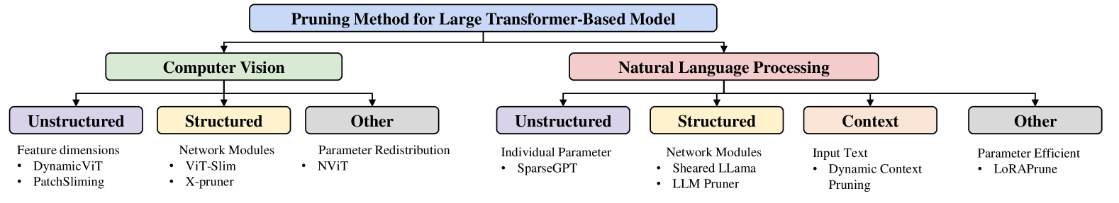
### Visual Description
## Diagram: Pruning Method for Large Transformer-Based Model
### Overview
This is a hierarchical diagram outlining different pruning methods for large transformer-based models. The diagram branches into two main application areas: Computer Vision and Natural Language Processing. Each of these areas is further categorized into sub-types of pruning, with specific examples listed under each sub-type.
### Components/Axes
The diagram consists of rectangular nodes with rounded corners, connected by arrows indicating a hierarchical relationship. The nodes are color-coded to distinguish different levels and categories.
* **Top Level (Blue):** "Pruning Method for Large Transformer-Based Model" - This is the root node.
* **Second Level (Green and Pink):**
* "Computer Vision" (Green)
* "Natural Language Processing" (Pink)
* **Third Level (Purple, Yellow, Grey, Peach):** These nodes represent categories of pruning methods within each application area.
* **Under Computer Vision:**
* "Unstructured" (Purple)
* "Structured" (Yellow)
* "Other" (Grey)
* **Under Natural Language Processing:**
* "Unstructured" (Purple)
* "Structured" (Yellow)
* "Context" (Peach)
* "Other" (Grey)
* **Fourth Level (Textual Lists):** These are lists of specific pruning techniques or characteristics associated with the third-level categories.
### Content Details
**Under "Computer Vision":**
* **Unstructured (Purple):**
* Feature dimensions
* DynamicViT
* PatchSliming
* **Structured (Yellow):**
* Network Modules
* ViT-Slim
* X-pruner
* **Other (Grey):**
* Parameter Redistribution
* NViT
**Under "Natural Language Processing":**
* **Unstructured (Purple):**
* Individual Parameter
* SparseGPT
* **Structured (Yellow):**
* Network Modules
* Sheared Llama
* LLM Pruner
* **Context (Peach):**
* Input Text
* Dynamic Context Pruning
* **Other (Grey):**
* Parameter Efficient
* LoRAPrune
### Key Observations
The diagram clearly separates pruning methods based on their application domain (Computer Vision vs. Natural Language Processing). Within each domain, pruning is further classified into common categories like "Unstructured," "Structured," and "Other." The "Natural Language Processing" domain also includes a specific "Context" category, suggesting a distinct approach for handling contextual information in NLP models. The diagram provides concrete examples of pruning techniques for each sub-category.
### Interpretation
This diagram serves as a taxonomy for understanding the landscape of pruning methods applied to large transformer-based models. It highlights that the choice of pruning method is often dictated by the application domain. The distinction between "Unstructured" and "Structured" pruning is a fundamental concept, with "Unstructured" typically referring to the removal of individual weights or parameters, and "Structured" referring to the removal of entire structures like neurons, channels, or layers. The inclusion of "Other" categories suggests that there are methods that do not fit neatly into the primary classifications. The "Context" category under NLP is particularly interesting, implying that methods specifically designed to leverage or prune contextual information are relevant in this domain. The specific examples provided (e.g., DynamicViT, SparseGPT, LoRAPrune) offer concrete instances of these pruning strategies, which would be valuable for researchers and practitioners looking to implement or compare different pruning techniques. The overall structure suggests a systematic approach to categorizing and understanding the diverse methods available for model compression in large transformer architectures.
</details>
Figure 5: The taxonomy of pruning methods used for Transformer models.
#### 4.1.2 Pruning for Transformer-Based Large Language Models
Pruning granularity. In response to the considerable parameter increase in the LLM era, there have been early attempts of pruning arise with the focus on unstructured and semi-structured pruning [143, 144, 145]. SparesGPT, for instance, conducts unstructured and semi-structured (mainly 2:4) pruning starting from OPT-175B [146] and BLOOM-176B [147] and achieve 50-60% sparsity with moderate perplexity increase and performance decrease on downstream datasets. This work demonstrates the feasibility of low-resource pruning in $>$ 100 B models with moderate sparsity.
Another line of work mainly focuses on the structured pruning method to achieve a more significant speed-up. Language structural pruning has been conducted at multiple granularities. For instance, Michel et al. [148] discuss the redundancy of attention head, Fan et al. [149] propose a task-specific extraction of pre-trained sub-networks, Santacroce et al. [150] focus on FFN layers, and Block Pruning [151] is introduced to prune MHA and FFN parameters separately. In comparison, CoFi [152] proposes a more comprehensive coarse- and fine-grained pruning method that learns to generate masks at different granularity, i.e., FFN layers, FFN intermediate dimensions, MHA layers, Attention heads, and hidden dimensions to encourage the optimization in the high sparsity domain. In this way, the pruning of a specific parameter can be determined at different granularity in an end-to-end learnable manner. When pruning the general domain pre-trained BERT model to typical downstream datasets, CoFi achieves more than $10\times$ speed-ups with a limited accuracy gap. Later, this method was extended to a larger decoder-based LLM with a 7B parameter size [30]. With a pre-defined model shape, the pruned model shows better instruction tuning performance than models of similar size but trained from scratch. Also, specifying the model configuration with uniform size avoids irregularities in model shape and further increases the inference throughput. In contrast to pre-defining the model shape, Ma et al. [29] propose first to identify groups of coupled structures considering the interdependency of parameters in FFN, MHA, and channel-wise groups and conduct the pruning process by group. Experiments at a relatively low compression rate (20%) demonstrate the varying effectiveness of these grouping strategies.
Pruning criteria. To determine the structure to be pruned, various metrics have been explored in the context of LLM pruning. For instance, Frantar et al. [143] follows [153] to find an optimal mask that can be used for weight reconstruction and uses Hessian Matrix (i.e., the second order indicator of loss change concerning the change of each parameter) to indicate the parameter importance, which is experimentally shown better than a magnitude criteria [154] and much faster than previous method AdaPrune [155]. In comparison, as noted by LLM Pruner [29], the first-order term should also be considered due to the shift of data used in the pruning process compared to the original language model training. Also, it proposes considering the weight importance at different levels and explores different ways of combining the importance information. Besides, Sun et al. [144] also explores the combination of magnitude and norm of the input activations as the pruning criteria, which lowers the computational cost used for Hessian computation.
Learning to prune. In addition to determining the importance of parameters using, one can also perform extra training, commonly with regularization on sparsity [156, 157]. In particular, the success of LLM as a multi-task language processor promotes the development of a pruning method that preserves this multi-task nature, as opposed to the task-specific trails that are more feasible in the traditional pretrain-finetune paradigm [152]. In response to this motivation, recent works such as SIMPLE [158], LLM Pruner [29] and Sheared LLama [30] incorporate the causal language modeling loss in the pruning objective. However, this “general pruning” strategy raises another issue of data selection in the pruning process, as the domain gap between pre-training and pruning may hinder the importance of estimation/performance recovery. As detailed in [30], a dynamic batch loading strategy is applied to adaptively input the data batch from a proper domain to balance the model performance as a multi-task learner.
Computation cost for parameter pruning. Considering the huge numbers of parameters, post-pruning retraining and parameter importance estimation may both generate a significant computational burden for large language models. In an early attempt, Frantar et al. [143] consider a one-shot strategy, i.e., only limited data are used to calibrate the Hessian Matrix in importance estimation, and no retraining was employed. From another perspective, LoRAPrune [159] shows that introducing parameter-efficient tuning such as Low-Rank Adaption can also decrease the computation cost in retraining while compensating for the performance degradation.
Context and token pruning. Different from the case in the computer vision domain, language sequence can be very long, and long-range reference or induction also calls for the expansion of input tokens (i.e., context) to prompt better language understanding. Also, since the inference cost of LLM is in quadratic complexity with respect to sequence length, this expansion greatly hinders the efficient inference of language models. To tackle these problems, methods have been proposed since BERT era to prune redundancy in context or context attention calculation. For context pruning, Kim et al. [160] propose to prune tokens across the Transformer layers progressively and improves the throughput by several folds on GLUE benchmark with less than 1% accuracy loss. Among the second line of research, various sparse attention techniques have been proposed, including local attention restricted to nearby tokens [161, 162, 163], introducing global tokens [164, 162], content-based token grouping [37, 163], and attention back tracking [165]. With the advance of the modeling capacity of LLM, the context input for LLM is also growing readily. To provide a more adaptive attention selection, Anagnostidis et al. [31] proposes a sparse sigmoid-based selection scheme. Also, erasing tokens from the key-value cache makes this method more hardware-friendly in a decoder-based language model. While the experiments are mainly conducted on modest size GPT-2 model [3], the empirical results that up to 80% of the context can be successfully pruned with negligible degradation in perplexity indicates an appealing potential to explore along this direction.
#### 4.1.3 Pruning for Transformer-Based Vision Model
TABLE V: comparison of representative pruning methods on vision Transformer DeiT-Base. The Speed-up ratio is calculated using the latency or throughput reported in the original paper. Top-1 Acc. is measured on ImageNet 1K. “/” indicates the keep ratio of dynamic tokens, and “-” denotes the pruning ratio of parameters.
| Models | Pruning Type | $\#$ Params | FLOPs | Speed Up | Top-1 Acc. (%) |
| --- | --- | --- | --- | --- | --- |
| DeiT-B | - | 86.6M | 17.6G | 1 $\times$ | 81.8% |
| DPS-DeiT-B [33] | Unstructured (Token) | 87M | 9.4G | 1.4 $\times$ | 81.5% |
| DynamicVIT-B/08 [166] | Unstructured (Token) | - | 13.3G | 1.2 $\times$ | 81.6% |
| S ${}^{2}$ ViTE-B [167] | Un- and Structured | 56.8M | 11.7G | 1.33 $\times$ | 82.2% |
| SAViT-50 [168] | Structured | 42.6M | 8.8G | 1.55 $\times$ | 82.5% |
| SAViT-70 [168] | Structured | 25.4M | 5.3G | 2.05 $\times$ | 81.7% |
| ViT-Slim [32] | Structured | 52.6M | 10.6G | - | 82.4% |
| WD-prining [169] | Structured and Early-Ex | 55.3M | 9.9G | 1.18 $\times$ | 80.76% |
| X-pruner [34] | Structured | 87M ${}^{\dagger}$ | 8.5G | - | 81.02% |
- ${}^{\dagger}$ The corresponding data is from [170].
TABLE VI: comparison of representative pruning methods on large language Transformer.
| Method | Pruning Type | Source Model | Compression | Speed | Comparison with |
| --- | --- | --- | --- | --- | --- |
| Rate | Up | Source Model | | | |
| SparseGPT [143] ${}^{\dagger}$ | Un- and semi-sturctured | OPT-175B [146] | 50-60% | 1.54-1.79 $\times$ | 8.38/8.34 |
| (WikiText2 ppl) | | | | | |
| Sheared LLama [30] | Structured | LLaMA2-7B [1] | 61.4% | - | 56.7%/64.6% |
| (11 datasets) | | | | | |
| LLM Pruner [30] | Structured | LLaMA2-7B [1] | 20% | 1.18 $\times$ | 60.07%/68.59% |
| (7 datasets) | | | | | |
| Dyna. Context Pruning [31] | Context | GPT-2 [3] | 80.35% ${}^{\star}$ | 1.2 $\times$ | +0.085 ppl |
| (Wiki and bookcorpus) | | | | | |
- ${}^{\dagger}$ Data is from 2:4 partial sparsity setting with GPU speedup [143].
- ${}^{\star}$ Compression rate refers to context tokens instead of parameters.
Token and feature pruning. The early exploration of pruning for vision Transformer pruning focuses on reducing information redundancy in feature space. In a preliminary study, Zhu et al. [171] propose learning the most informative feature dimensions and neglecting the remaining dimensions in the inference time. This is achieved by learning a diagonal real-value feature mask during pre-training with a sparsity regularizer and obtaining the hard feature mask using a defined threshold. From a different perspective, given the fact that token features in late ViT layers are quite similar in feature embedding, patch slimming [33] method is proposed to prune the patches from the output layer to the input layer. In particular, for each layer, it evaluates the impact of a patch on the final output feature and removes less important ones. Besides determining the patch importance by training dataset statistics, token sparsification can also be achieved by inserting a light-weight prediction network to indicate the importance of the input patches [33, 166, 172, 173, 167]. Note that since the self-attention can accept the token sequence regardless of its length, unstructured pruning of input tokens can be easily implemented in a hardware-friend manner for these token pruning methods. Furthermore, similar techniques are adopted in other Transformer-based vision models such as DETR [174] to promote focus on object tokens [175, 176].
Structured pruning. Apart from the redundancy in feature dimension and tokens, the heavy burden of matrix computation is another important axis to improve model efficiency. In an early work, [167] proposes to selectively optimize for sparsity by obtaining unstructured subnetworks and structured pruning for attention heads, besides importance-based token selection. [169] develops a structural pruning method to reduce the network’s width by pruning linear projection matrices as well as attention heads, together with depth pruning with inserted early-exit classifiers at each layer. Later on, more works emerged to explore the collaborative effect of parameter pruning across different Transformer modules. In [177], a Hessian-based criteria is proposed to evaluate the parameter importance globally over learnable parameters. Together with the parameter redistribution strategy that promotes shorter latency, this method can also introduce novel efficient ViT structures named NViT. With an emphasis on speeding up continuous structure search, Chavan et al. [32] perform a single-shot architecture search for all the ViT components with significantly fewer GPU hours needed. Also, by incorporating the interactions between the components, Zheng et al. [168] manage to introduce adaptively the pruning ratio for each component, adding another degree of freedom in pruning. More recently, Yu et al. [34] propose to use class labels to optimize the fully differentiable pruning operation at each layer.
#### 4.1.4 Discussion
Pruning serves as a fundamental way to reduce the computation burden of the pre-trained Transformer. Traditionally, this is achieved in an orthogonal manner by pruning input features or network parameters. In particular, we notice that different pruning methods can biasedly benefit particular application purposes. For large language models, structured network pruning fits more in the setting when a modest length (e.g., several thousand tokens) is used as input to speed up inference, as the defined hardware-friendly model shape has been proven to realize a good trade-off between acceleration and perplexity decrease [30]. In comparison, context pruning or sparse attention methods deserve more attention when context length gets longer, and the ceiling of pruning ratio for context for LLMs (e.g., 7B or more) has not been determined in a detailed manner, which is an interesting direction to explore. For vision Transformers, the development of pruning methods has systematically tackled each angle of model design, making the current pruning process more flexible and closer to a continuous structural search task, which can be an excellent reference to the development of language domains. The training cost is another critical axis to consider in the pruning of large models, especially when incremental LLM pre-training is considered a component of the pruning process. Therefore, developing training-efficient pruning methods is attracting more attention. This requires the parameter (or block) sensitivity to be estimated more accurately using limited data or the information stored in hidden features during training/inference to be explored more in-depth.
### 4.2 Efficient Architecture
Transformer [11] has become the de facto backbone architecture to develop various large vision and language models (LVMs and LLMs), making it possible to scale to billions of parameters. In this section, we review the efficient architecture design of large Transformer-based models in both vision and language domains, i.e., efficient design on mainstream architecture, attention mechanism and feed forward network. Notably, here we also discuss the recently proposed Mamba [178], a general sequence model backbone that integrates selective state space models (SSMs) into a simplified end-to-end neural network architecture. In this section, we consider it as an efficient design for subquadratic-time architectures.
#### 4.2.1 Representative Transformer-Based Models
Table VII presents the model cards of several representative LLMs and LVMs with public details. Vanilla Transformer [11] is based on the encoder-decoder architecture [133]. In this architecture, the encoder stacks multi-head self-attention layers to encode the input sequence into latent representations, while the decoder performs cross-attention on these representations and generates target sequences in an autoregressive manner. BERT [91] is designed to pre-train deep bidirectional representations from unlabeled text by considering both left and right context in all layers. GPT-series models [4, 2] have effectively demonstrated the power of in-context learning using decoder-only architectures [147, 179, 180]. These decoder architectures incorporate unidirectional attention masks to ensure that each input token can only attend to previous tokens, including itself. The input and output tokens are processed in a similar manner within the decoder. In the following, we will provide separate reviews from the perspectives of CV and NLP on the current structural innovations in Transformer-based architectures.
#### 4.2.2 Language Domain
The self-attention mechanism in conventional Transformer architectures often faces quadratic computational complexity. This poses a challenge for training and making inferences with long input sequences. To enhance efficiency, current innovations in the mainstream can be classified into three categories: optimizations targeting the attention mechanism, the direct replacement of attention with more efficient architectures, and enhancements focused on the FFN component.
Attention innovation. Various efficient Transformer variants have been proposed to reduce the computational complexity of the attention mechanism by incorporating structural priors on attention, such as sparsity [181, 182, 183, 184, 185, 186]. For example, Reformer [37] approximates full attention computation using locality-sensitive hashing, reducing the complexity from $\mathcal{O}(N^{2})$ to $\mathcal{O}(N\log N)$ . Other techniques include pooling-based compression [185], clustering methods [184, 187] that apply k-means clustering to learn dynamic sparse attention regions, and Longformer [188], which combines local windowed attention with task-motivated global attention. Chelba et al. [189] proposes truncating the target-side window based on an $N$ -gram assumption, restricting the self-attention mechanism to use only the previous $N-1$ tokens. Additionally, locally banded sparse attention methods, such as Factorized Attention [183], have been adopted in models like GPT-3 [4].
Other methods have been proposed to reduce the computational complexity of the attention mechanism using linear attention. Performer [190] introduces fast attention via positive orthogonal random features, which is a scalable kernel method for approximating softmax attention kernels. This approach can efficiently model kernelizable attention mechanisms beyond softmax and comes with strong theoretical guarantees, including nearly unbiased estimation of the attention matrix, uniform convergence, and low estimation variance. Linear Transformer [191] reformulates self-attention as a linear dot-product of kernel feature maps. It uses kernels $\frac{\phi(q_{i})\phi(k_{j})}{\sum_{n=1}^{|x|}\phi(q_{i})\phi(k_{n})}$ to replace the softmax function and takes advantage of the associativity property of matrix products to reduce the computational complexity from $\mathcal{O}(N^{2})$ to $\mathcal{O}(N)$ .
Moreover, there have been studies [35, 192, 193] exploring the concept of multi-query attention, where different heads share the same linear transformation matrices for the keys and values, as proposed by Shazeer et al. [193]. This approach offers significant computational savings with only a minimal impact on model quality. To further strike a balance between multi-query attention and multi-head attention, GQA et al. [194] introduces the concept of grouped attention heads, where heads within the same group share identical transformation matrices.
TABLE VII: Model cards of several representative Transformer-based LLMs and LVMs with public configuration details. Here $d_{model}$ is already expanded by expansion ratio.
| Models | Arch. | $\#$ Params | Layer | Head | $d_{model}$ |
| --- | --- | --- | --- | --- | --- |
| Natural Language Processing | | | | | |
| BERT [91] | Encoder | 0.1B-0.3B | 12-24 | 12-16 | 3072-4096 |
| PaLM [35] | Decoder | 9B-540B | 32-118 | 16-48 | 4096-18432 |
| Gopher [179] | Decoder | 4M-280B | 8-80 | 16-128 | 512-16384 |
| BLOOM [147] | Decoder | 0.6B-176B | 24-70 | 16-112 | 1024-14336 |
| GPT3 [4] | Decoder | 175B | 96 | 96 | 12288 |
| GLM-130B [195] | Decoder | 130B | 70 | 96 | 12288 |
| Chinchilla [196] | Decoder | 70B | 80 | 64 | 8192 |
| LLaMA [1] | Decoder | 7B-65B | 32-80 | 32-64 | 4096-8192 |
| Falcon [180] | Decoder | 40B | 60 | 64 | 8192 |
| T5 [133] | En.-De. | 11B | 24 | 128 | 1024 |
| Computer Vision | | | | | |
| ViT [128] | Encoder | 86M-0.6B | 12-32 | 12-16 | 3072-5120 |
| DeiT [127] | Encoder | 5M-86M | 12 | 3-12 | 768-3072 |
| TNT [197] | Encoder | 6M-66M | 12 | 3-10 | 768-2560 |
| PVT [198] | Pyramid | 13M-61M | 12-45 | 8 | 2048 |
| CMT [199] | Pyramid | 10M-75M | 24-40 | 8 | 1324-2432 |
| Swin [38] | Pyramid | 29M-0.2B | 16-28 | 24-48 | 3072-6144 |
FlashAttention [200] offers an innovative approach to optimizing the speed and memory utilization of attention modules on GPUs. It focuses on an Input/Output (IO)-aware perspective, making better use of the fast memory SRAM by dividing the input into blocks. This optimization technique has already been integrated into various platforms [201, 202, 203, 204, 205] developed for training LLMs.
Non-Transformer architecture. Recent research has focused on developing new architectures for language modeling, including parameterized state space models [206, 207, 208, 209], long convolutions [210], and the incorporation of recurrent models [211, 212, 36, 213], which come with strong inductive biases. In particular, Gu et al. [206] introduces the S4 model, based on a novel parameterization for the SSM [214, 215], which involves conditioning matrix A with a low-rank correction, making it stably diagonalizable. This reduces the SSM to the well-studied computation of a Cauchy kernel [216]. The GSS model [207] further extends the use of gating units to the state space model family, and it is observed that employing gating units leads to dimensionality reduction when performing FFT operations, which addresses a major bottleneck in training speed. Hyena [210] trains a recurrence of gating units and implicitly parametrized long convolutions, which serves as an attention-free drop-in replacement for the traditional Transformer architecture. Ma et al. [213] introduces MEGA, a single-head gated attention mechanism enhanced with exponential moving average. This mechanism aims to integrate the inductive bias of position-aware local dependencies into the position-agnostic attention mechanism.
Peng et al. [217] proposes RWKV based on the fact that Recurrent Neural Networks (RNNs) show linear scaling in memory and computational requirements but encounter limitations in parallelization and scalability. They leverage a linear attention mechanism, specifically replacing the quadratic QK attention with a scalar formulation that has linear cost. Additionally, they redefine recurrence and sequential inductive biases to parallelize computations during training while maintaining constant computational and memory complexity during inference.
<details>
<summary>x13.png Details</summary>
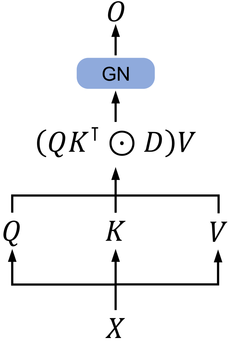
### Visual Description
## Diagram: Attention Mechanism Flow
### Overview
This diagram illustrates a simplified flow of an attention mechanism, likely within a neural network context. It shows how an input `X` is transformed into query (`Q`), key (`K`), and value (`V`) representations, which are then used in a calculation involving matrix multiplication, element-wise multiplication with a diagonal matrix `D`, and finally a transformation by a "GN" module to produce an output `O`.
### Components/Axes
This diagram does not contain axes or legends in the traditional sense of a chart. The components are:
* **Input `X`**: Represented by a single letter 'X' at the bottom, with an arrow pointing upwards, indicating it's the initial input.
* **Query `Q`**: Represented by a single letter 'Q' on the left, with an arrow pointing upwards from a horizontal line originating from `X`.
* **Key `K`**: Represented by a single letter 'K' in the center, with an arrow pointing upwards from a horizontal line originating from `X`.
* **Value `V`**: Represented by a single letter 'V' on the right, with an arrow pointing upwards from a horizontal line originating from `X`.
* **Intermediate Calculation `(QKᵀ ⊙ D)V`**: This is a mathematical expression enclosed in parentheses, indicating a sequence of operations.
* `Q`: Query matrix.
* `Kᵀ`: Transpose of the Key matrix.
* `⊙`: Element-wise multiplication (Hadamard product).
* `D`: A diagonal matrix.
* `V`: Value matrix.
* The entire expression represents the core attention calculation.
* **"GN" Module**: A light blue rounded rectangle containing the text "GN". This likely represents a normalization or a specific layer type (e.g., Group Normalization, Layer Normalization, or a custom module). An arrow points upwards into this module.
* **Output `O`**: Represented by a single letter 'O' at the top, with an arrow pointing upwards from the "GN" module, indicating it's the final output of this process.
### Detailed Analysis or Content Details
The diagram depicts the following flow of operations:
1. An input `X` is processed to generate three distinct representations: `Q`, `K`, and `V`. These are shown as originating from `X` via separate upward arrows, suggesting linear transformations or embeddings.
2. The `Q` and `K` representations are used to compute attention scores. This is indicated by the expression `QKᵀ`.
3. The result of `QKᵀ` is then element-wise multiplied by a diagonal matrix `D`. This step often involves scaling or masking the attention scores. The symbol `⊙` explicitly denotes element-wise multiplication.
4. The result of the element-wise multiplication is then multiplied by the `V` representation. This weighted sum of values forms the output of the attention mechanism.
5. The output of the attention calculation `(QKᵀ ⊙ D)V` is then passed through a module labeled "GN".
6. The "GN" module processes its input and produces the final output `O`.
### Key Observations
* The diagram represents a common pattern in attention mechanisms, particularly in transformer architectures, where queries, keys, and values are derived from an input.
* The inclusion of `D` and the `⊙` operator suggests a mechanism for modifying or masking the attention scores before they are applied to the values. This could be for positional encoding, padding masks, or other forms of attention control.
* The "GN" module indicates a post-attention processing step, likely for stabilization or feature refinement.
### Interpretation
This diagram illustrates a fundamental component of many modern deep learning models, especially in natural language processing and computer vision. The process shown is a form of scaled dot-product attention, potentially with an added masking or scaling factor represented by `D`.
* **What the data suggests or demonstrates**: The diagram demonstrates how an input signal `X` can be decomposed and recombined through a series of matrix operations and a normalization step to produce a contextually aware output `O`. The core idea is that `Q` and `K` determine the "importance" or "attention" of different parts of the input, and these importance weights are then used to aggregate the `V` representations.
* **How the elements relate to each other**:
* `X` is the foundational input from which `Q`, `K`, and `V` are derived.
* `Q` and `K` are used together to compute similarity scores (attention weights).
* `D` modifies these attention weights.
* The modified attention weights are then applied to `V` to create a weighted sum.
* The "GN" module acts as a subsequent processing layer on this weighted sum.
* `O` is the final output after all transformations.
* **Any notable outliers, trends, or anomalies**: The diagram is a schematic representation and does not contain numerical data, so there are no outliers or trends in the data itself. However, the presence of `D` and the `⊙` operator is a notable detail, as it signifies a deviation from the simplest form of scaled dot-product attention (which typically only involves scaling by `sqrt(d_k)`). This suggests a more sophisticated attention mechanism is being depicted. The "GN" module is also a specific choice for post-attention processing, implying a particular architectural design.
</details>
(a) Parallel representation.
<details>
<summary>x14.png Details</summary>
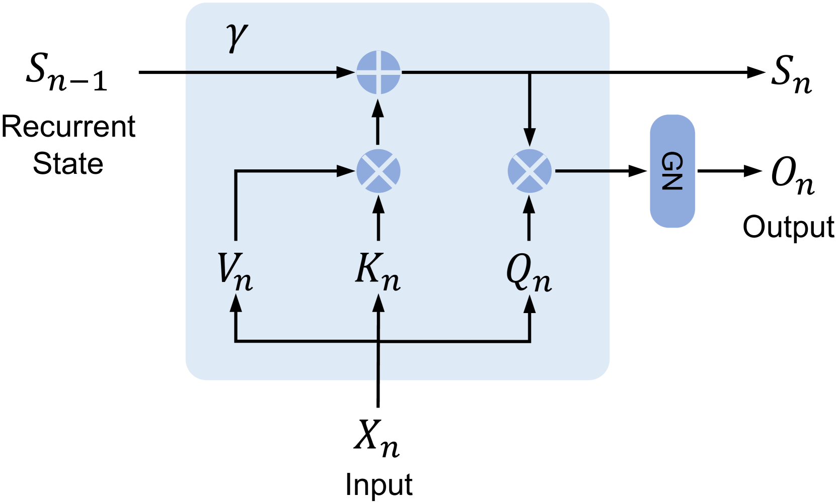
### Visual Description
## Diagram: Recurrent Neural Network Cell Structure
### Overview
This diagram illustrates a computational cell within a recurrent neural network (RNN). It depicts the flow of information and the operations performed at a specific time step 'n', taking into account the previous state 'S_{n-1}' and the current input 'X_n'. The cell produces a new recurrent state 'S_n' and an output 'O_n'.
### Components/Axes
The diagram does not feature traditional axes or legends as it is a schematic representation of a computational process. The key components and their labels are:
* **S_{n-1}**: Represents the recurrent state from the previous time step (n-1). It is shown as an input on the left side of the diagram.
* **Recurrent State**: A textual label accompanying 'S_{n-1}', clarifying its meaning.
* **X_n**: Represents the input at the current time step 'n'. It is shown as an input at the bottom of the diagram.
* **Input**: A textual label accompanying 'X_n', clarifying its meaning.
* **V_n**: A variable or intermediate state derived from 'X_n'. It is shown as an input to a multiplication operation.
* **K_n**: A variable or intermediate state derived from 'X_n'. It is shown as an input to a multiplication operation.
* **Q_n**: A variable or intermediate state derived from 'X_n'. It is shown as an input to a multiplication operation.
* **γ (gamma)**: A parameter or operation applied to the recurrent state 'S_{n-1}'. It is shown as an input to an addition operation.
* **⊕ (Plus Symbol within a Circle)**: Represents an addition operation.
* **⊗ (Cross Symbol within a Circle)**: Represents a multiplication operation.
* **GN**: Represents a "Gated Network" or a similar gating mechanism. It takes an input and produces an output.
* **S_n**: Represents the new recurrent state at the current time step 'n'. It is an output of the cell.
* **O_n**: Represents the output at the current time step 'n'. It is an output of the cell.
* **Output**: A textual label accompanying 'O_n', clarifying its meaning.
The entire cell's computation is enclosed within a light blue shaded region.
### Detailed Analysis or Content Details
The diagram illustrates the following computational flow:
1. **Input Processing**: The input 'X_n' is processed to generate intermediate variables 'V_n', 'K_n', and 'Q_n'. The exact nature of this processing is not specified but is implied to be a transformation of 'X_n'.
2. **State Update Calculation**:
* The previous recurrent state 'S_{n-1}' is combined with a parameter 'γ'.
* 'V_n' is multiplied by 'K_n' (⊗ operation).
* The result of 'S_{n-1}' and 'γ' is added to the result of the 'V_n' * 'K_n' multiplication (⊕ operation). This forms a component of the new state 'S_n'.
3. **Output Calculation**:
* The result of 'S_{n-1}' and 'γ' is also multiplied by 'Q_n' (⊗ operation).
* This product is then passed through the "GN" (Gated Network) component.
* The output of the "GN" component is the final output 'O_n'.
4. **New State Generation**: The result from the addition operation (from step 2) directly becomes the new recurrent state 'S_n'.
### Key Observations
* The diagram represents a modular computational unit, likely a component of a more complex RNN architecture such as a Gated Recurrent Unit (GRU) or a Long Short-Term Memory (LSTM) cell, or a custom variant.
* The use of multiplication (⊗) and addition (⊕) symbols indicates element-wise operations or matrix multiplications, depending on the dimensionality of the states and inputs.
* The "GN" block suggests a gating mechanism that controls the information flow to the output.
* The diagram clearly separates the calculation of the next recurrent state ('S_n') from the generation of the observable output ('O_n').
### Interpretation
This diagram outlines a specific type of recurrent neural network cell that processes sequential data. The structure suggests a mechanism for selectively updating and propagating information through time.
* **Information Flow and Memory**: The recurrent state 'S_{n-1}' acts as a form of memory, carrying information from previous time steps. The operations involving 'γ', 'V_n', 'K_n', and 'Q_n' suggest that the cell dynamically decides how much of the past state to retain and how to incorporate the current input. The addition operation likely combines the "remembered" past state with a "newly computed" component derived from the input.
* **Gating Mechanisms**: The multiplication operations and the "GN" block are indicative of gating mechanisms. These gates are crucial in RNNs for controlling the flow of information, preventing vanishing or exploding gradients, and allowing the network to learn long-term dependencies. The multiplication of 'S_{n-1}' with 'γ' and the subsequent addition could be interpreted as a form of "forgetting" or "updating" the previous state. The multiplication with 'Q_n' and passing through "GN" for the output 'O_n' suggests that the output is a filtered or transformed version of the internal state, controlled by the input-derived 'Q_n'.
* **Purpose**: Such a cell is designed to learn patterns in sequential data, where the output at any given time step depends not only on the current input but also on the history of inputs. The specific arrangement of operations and variables would determine the cell's capacity to model different types of temporal dependencies. For instance, if 'γ' is a learned parameter, it could act as a forget gate. If 'V_n', 'K_n', and 'Q_n' are derived through learned transformations of 'X_n', they would function as input gates or update gates. The "GN" block could be a final activation or another gating layer.
In essence, this diagram provides a blueprint for a sophisticated computational unit capable of processing sequential information by maintaining an internal state and dynamically modulating the influence of past information and current inputs on both the state update and the output.
</details>
(b) Recurrent representation.
Figure 6: Dual form of RetNet (image from [36]).
Furthermore, Retentive Network (RetNet) [36] theoretically derives the connection between recurrence and attention and proposes the retention mechanism for sequence modeling. This mechanism supports three computation paradigms, namely parallel, recurrent, and chunkwise recurrent, achieving training parallelism, low-cost inference, and good performance simultaneously. The parallel representation (also depicted in Figure 5(a)) of retention is:
$$
\displaystyle Q=(XW_{Q})\odot\Theta, \displaystyle\quad K=(XW_{K})\odot\overline{\Theta},\quad V=XW_{V} \displaystyle\Theta_{n}=e^{in\theta}, \displaystyle\quad D_{nm}=\left\{\begin{aligned} &\gamma^{n-m},&n\geq m\\
&0,&n<m\\
\end{aligned}\right. \displaystyle\mathrm{Rete} \displaystyle\mathrm{ntion}(X)=(QK^{\intercal}\odot D)V \tag{10}
$$
where $\overline{\Theta}$ is the complex conjugate of $\Theta$ , and $D\in\mathbb{R}^{|x|\times|x|}$ combines causal masking and exponential decay along relative distance as one matrix. This parallel representation enables RetNet to train the models with GPUs efficiently. The recurrent version of retention (Figure 5(b)) is favorable for inference and can be written as (for $n$ -th timestep):
$$
\displaystyle S_{n}=\gamma S_{n-1}+K_{n}^{\intercal}V_{n} \displaystyle\mathrm{Rete}\mathrm{ntion}(X_{n})=Q_{n}S_{n},\quad n=1,\cdots,|x| \tag{11}
$$
where $Q,K,V,\gamma$ are the same as in Eq. 10.
More recently, Gu et al. [178] have highlighted the limitations of previous structured SSMs in effectively modeling discrete and information-dense data, such as text. In response, they propose Mamba, consisting a novel class of selective mechanisms and hardware-aware designs that enable linear scalability to billions of parameters, while maintaining computational efficiency and achieving strong performance. Specifically, in comparison to the H3 [208] block, the Mamba model replaces the first multiplicative gate with an activation function. Additionally, Mamba incorporates an SSM into the main branch, distinguishing it from the MLP block in transformer. Building upon the foundation of Mamba, researchers are further unlocking the potential of SSMs for scaling by exploring new techniques, such as combining SSMs with Mixture of Experts (MoE) [218] or introducing methods to enhance the flow of hidden information [219] between layers in SSMs.
FFN innovation. Large and sparse FFNs such as Mixture-of-Experts (MoE) [220, 221, 222, 223, 224, 225] have been effective in scaling up Transformer-based models for pre-training LLMs. They replace a single FFN module with multiple equally-sized modules (experts) and activate only a few experts based on the input. This selective activation of FFN improves generalization performance while maintaining fixed training and inference costs. Liu et al. [226] further finds a simpler selection method known as Avg-K, which selects blocks based on their mean aggregated hidden states. This method achieves lower perplexity in language model pre-training compared to existing MoE architectures such as Switch Transformer [222] and HashLayer [223].
Romero et al. [227] presents Continuous Kernel Convolution (CKConv) for handling arbitrarily long sequences in a parallel manner within a single operation. CKConv formulates convolutional kernels as vector-valued continuous functions parameterized by a small MLP instead of a sequence of independent weights. This MLP takes a time-step as input and generates the value of the convolutional kernel at the corresponding position, allowing the generation of kernels at different resolutions and arbitrarily sizes.
PaLM [35] and LLaMA [1] both utilize the SwiGLU Activation (Swish( $xW$ ) $\dot{x}V$ ) for original FFN intermediate activations. This choice is based on the observation that SwiGLU activations have been shown to substantially enhance quality in compute-equivalent experiments [228] when compared to standard activation functions such as ReLU, GeLU, or Swish [228]. It’s important to note that using SwiGLU does require three matrix multiplications in the MLP instead of two.
TABLE VIII: Model comparison from training parallelization (TP), inference cost (Time), and memory complexity (Memory). Here $N$ and $d$ denote the sequence length and feature dimension, respectively.
| Architectures | TP | Time | Memory |
| --- | --- | --- | --- |
| RNN [229] | ✘ | $O(Nd)$ | $O(d)$ |
| Transformer [11] | ✔ | $O(N^{2}d)$ | $O(N^{2}+Nd)$ |
| Linear Attention [191] | ✔ | $O(Nd^{2})$ | $O(Nd+d^{2})$ |
| H3 [208] | ✔ | $O(Nd(\log N+d))$ | $O(Nd)$ |
| S4 [206] | ✔ | $O(Nd^{2})$ | $O(Nd)$ |
| Hyena [210] | ✔ | $O(Nd(\log N+d))$ | $O(N\log N\cdot d)$ |
| Reformer [37] | ✔ | $O(N\log N\cdot d)$ | $O(N\log N+Nd)$ |
| Performer [190] | ✔ | $O(Nd^{2}\log d)$ | $O((Nd+d^{2})\cdot\log d)$ |
| RWKV [217] | ✔ | $O(Nd)$ | $O(d)$ |
| RetNet [36] | ✔ | $O(Nd^{2})$ | $O(d^{2})$ |
| Mamba [178] | ✔ | $O(Nd)$ | $O(d)$ |
#### 4.2.3 Vision Domain
Dosovitskiy et al. [128] first introduces the Vision Transformer (ViT) primarily designed for image classification tasks. In the ViT model, the input image is initially divided into a sequence of fixed-length tokens, which are then processed through multiple Transformer layers to capture global relationships among the tokens. Similar to the challenges faced in the language domain, the self-attention mechanism with quadratic computational complexity is one of the major hurdles for training and inference in Transformer-based architectures applied to vision tasks. Many dense prediction tasks, such as object detection and image segmentation, often require higher-resolution inputs, necessitating the manual design of efficient architectures to handle these challenges. To address these issues, novel architectures like PVT [198] and Swin [198] have been proposed. These architectures incorporate hierarchical (pyramid) structures with multiple stages, effectively overcoming the challenges of adapting the original isotropic ViT [128] to various dense prediction tasks in computer vision.
In the following, we will delve into papers that focus on improving the efficiency of ViTs, including efforts to enhance local information processing [199, 230, 231, 232, 233, 234, 235], simplify the attention mechanism [236, 237, 238, 239, 240], and explore alternative modules that can replace or work alongside attention mechanisms [241, 39, 242, 243, 244], etc.
Enhancing locality. T2T-ViT [245] leverages token transformations to reduce token length by iteratively aggregating neighboring tokens to one token. LeViT [246] and MobileViT [247] employ hybrid architectures with stacked convolution layers, efficiently reducing the number of features through the first layer. TNT [197] further divides original ViT’s 16 $\times$ 16 patches into smaller 4 $\times$ 4 patches for capturing local information. CrossViT [234] processes small-patch and large-patch tokens separately, fusing them through multiple attention mechanisms. Twins [248] alternates between local and global attention layers for improved performance. RegionViT [249] introduces regional tokens and local tokens, enhancing local context with global information. KVT [250] introduces the k-NN attention to utilize locality of images patches and ignore noisy tokens by only computing attentions with top-k similar tokens. CMT [199] applies depth-wise convolutions to augment local patterns in the attention map and intermediate activation of the FFN. Pan et al. [251] proposes HiLo attention to disentangle the high/low frequency patterns in an attention layer by separating the heads into two groups, each equipped with specialized operations that focus on local windows.
Faster attention. Parmar et al. [236] introduces restrictions on the attention mechanism to focus on local neighborhoods. Swin [38] and Cswin [252] incorporate local attention within a window and introduce a shifted window partitioning method to enable cross-window connections. Shuffle Transformer [253] and Msg-Transformer [254] employ spatial shuffle operations as alternatives to shifted window partitioning, facilitating cross-window connections. FasterViT [237] introduces hierarchical attention, breaking down global self-attention into multi-level attention components. This approach combines local window attention and hierarchical attention to achieve global information propagation while reducing computational costs. FLatten Transformer [255] integrates depth-wise convolution in conjunction with linear attention mechanisms to address the challenge of maintaining diversity in output features across different positions.
Attention-free architecture. AFT [256] pioneers an innovative approach by combining key and value elements with learned position biases, followed by element-wise multiplication with the query. This operation’s distinctive feature is its linear memory complexity concerning both context size and feature dimension, making it compatible with large input and model sizes. GFnet [257] presents an alternative by replacing traditional attention mechanisms with Fast Fourier Transform (FFT), frequency gating, and inverse FFT for rapid token mixing. Additionally, some architectures have been entirely based on pure multi-layer perceptrons (MLPs) [258, 40, 259, 260, 243, 244], without using convolutions or self-attention mechanisms. Yu et al. [39] proposes MetaFormer as a general architecture abstracted from ViTs without specifying the token mixer. By employing basic token mixing, primarily through non-parametric pooling, MetaFormer achieves satisfactory performance.
Inspired by the efficient hardware-aware designs of Mamba in NLP, Zhu et al. [261] propose a novel generic vision backbone called Vim with bidirectional Mamba blocks. Different from the sequential nature of language, representing visual data in SSMs presents challenges primarily due to their sensitivity to spatial position. To address this, Vim introduces position embeddings to mark image sequences and compresses visual representations using bidirectional SSM. Following the architectures of ViT [12] and DeiT [26], Vim initially employs a 16×16 kernel size projection layer to obtain a 1-D sequence of non-overlapping patch embeddings. Simultaneously, Liu et al. [262] propose the visual state space model (VMamba), which introduces the Cross-Scan Module (CSM) to traverse the spatial domain and convert any non-causal visual image into ordered patch sequences, thereby addressing the inherent direction-sensitive issue. Following the architecture of Swin [136], VMamba begins the process by partitioning the input image into patches using a stem module, without further flattening the patches into a 1-D sequence.
NAS. Indeed, the quest for optimizing Transformer architectures extends to the realm of neural architecture search (NAS). Various models, including Scaling-ViT [263], ViTAS [264], AutoFormer [265] and GLiT [266], have emerged as products of NAS-driven design, demonstrating the potential for more efficient and effective Transformer architectures.
#### 4.2.4 Discussion
Transformer models consistently achieve state-of-the-art results across various tasks, but the cost of training these models, especially on long sequences, can be prohibitive. Table VIII concludes several papers that propose improvements to the attention mechanism from three different dimensions. While using linear attention can help reduce the computational complexity of the attention mechanism, it struggles to effectively encode position information, leading to a potential decrease in model performance. Models like RWKV [217], RetNet [36] and Mamba [178], which generate outputs recursively similar to RNNs, present a promising direction for further exploration. These models only need to refer to the previous state during decoding, significantly improving decoding efficiency by avoiding the need to revisit all previous states, a characteristic of conventional Transformers. Additionally, they can encode entire sentences in parallel, enabling highly parallel and efficient training.
In contrast to NLP tasks, high-level vision tasks place a strong emphasis on the network’s ability to capture local details, contextual information, and multi-scale features for dense predictions [198]. Several studies [267, 39] have also demonstrated that the self-attention mechanism is not always indispensable for feature extraction in vision tasks. In the exploration of pure vision tasks, the possibility of directly omitting the attention module is a worthwhile avenue for further research. However, it’s worth noting that attention and cross-attention modules still play a crucial role in integrating visual features with other modalities [15]. Therefore, the quest for faster attention algorithms remains a valuable research direction.
## 5 Specialized Approaches
In addition to quantization, distillation, pruning, and novel network architectures, there are several other model compression and acceleration approaches including tensor decomposition, early exiting, and speculative sampling.
Tensor decomposition. Tensor or matrix decomposition aims to decompose a large tensor or matrix into smaller ones in order to reduce the number of parameters and computational costs. This approach was first introduced into the compression of fully-connected layers and convolutional networks [268, 269]. In terms of large language models, Tensor decomposition is utilized for simplifying model weight or embedding layers. Edalati et.al [270] is the first attempt to use Kronecker decomposition for compressing generative language models. This work represent weight matrix with two smaller matrices using Kronecker decomposition and achieves lossless $1.5\times$ compression of GPT2. LoRD [271] further uses low rank decomposition to compress code LLMs. And TSVD [272] compresses linear mappings in Transformers using SVD and constrain $U$ and $V$ matrices in ternary format. In addition to model weights, TensorGPT [273] proposes to compress embedding layers and achieves more than $3\times$ compression factor with lossless performance.
Early exiting. Early exiting can dynamically allocate different resources for each input sample and maintain the original performance. This technology has been successfully used in information retrieval system [274] and convolutional networks [275]. Many early exiting technologies have been proposed for encoder-only Transformers [276, 277, 278, 279]. The key problem in early exiting is determining when to exit. The existing works mainly utilize intrinsic confidence measures [276], routing in advance [280], or training a early-exit classifier [281]. For Transformers with decoders, several works have been proposed. For example, Elbayad et.al [282] introduces the depth-adaptive Transformer for accelerating machine translation. CALM [283] proposes to dynamically allocate different computational resources for different input and timesteps, achieving speedups of up to $3\times$ on T5 encoder-decoder model. Additionally, SkipDecoder [284] bypasses tokens in lower layers to middle layers in order to enable batch inference and reuse KV caching, achieving inference speedups of $2\times$ to $5\times$ on OPT models.
Speculative sampling. Speculative sampling, a special acceleration approach for Transformer decoding, computes several tokens in parallel [285, 286]. In large language models, decoding $K$ tokens requires $K$ runs of the model – a slow process. Taking the reference tokens generated from smaller models, speculative sampling runs these tokens in parallel to significantly accelerate the decoding process. Moreover, the rejection scheme [286] can preserve the distribution of the original LLM so that speculative sampling is theoretically lossless. For example, Yang et.al [287] further take the input text as reference tokens without introducing extra models. And LLMCad [288] introduces an on-device inference engine for LLMs with speculative sampling as a key technology.
Discussion. This section has reviewed the methods that differ from those mentioned earlier, covering tensor decomposition, early exiting, and speculative sampling. These methods do not change the basic operations but instead accelerate model inference by modifying the network connections. Tensor decomposition approximates the original weights with low-rank ones, potentially leading to performance degradation. Early exiting makes predictions by adaptively allocating resources on a per sample basis. And speculative sampling considers the specialization of decoders and can accelerate decoding in a lossless manner. These special methods inspire future development of new algorithms for accelerating LLMs or LVMs.
## 6 Conclusions and Future Directions
In this survey, we systematically investigate the compression methods for Transformer models. Compared with compression method for conventional models, there are unique considerations when compressing Transformer models. Unlike other architectures such as CNN or RNN, the Transformer adopts a unique architecture design with alternative attention and FFN modules. This necessitates specifically tailored compression methods for optimal compression rates. Moreover, the efficiency of compression methods becomes particularly crucial for large models. Certain model compression methods require substantial amounts of computational resources, making them potentially prohibitive for such models. This survey aims to encompass the majority of recent works pertaining to Transformers and articulate a comprehensive roadmap for their compression. Subsequently, we delve into the interconnections among various methods, address post-challenges, and outline directions for future research.
Relationship between different compression methods. Different compression methods can be used together to obtain an extremely efficient architecture. A conventional sequence is to firstly define a new architecture with efficient operations. Any redundant components (e.g., attention head, layers) are then removed to reduce the model size. For practical hardware implementation, quantizing weights or activations to lower bits is imperative. The choice of required bits depend on not only the tolerance of error, but also hardware design. As an illustration, Int8 computation is efficiently optimized on Nvidia A100 GPU, but it lacks support on the older Tesla P100 GPU. Distillation commonly serves as a training strategy that applies during the fine-tuning phases of both pruning and quantization. Combining different compression strategies is a promising direction to explore for achieving extremely high compression rates. Although detailed exploration has been conducted into conventional models like CNN [9, 289], Transformer models have more complicated architectures and higher computational costs. Finding a suitable combination strategy via joint search is a challenging task.
Training-efficient compression strategy. In contrast to compressing conventional models, there is a heightened emphasis on the computational cost of compression methods.
Different from compression for conventional models, the cost of compressing large Transformers has been put on higher priority. Large Transformers are currently trained on vast datasets using significant computational resources. For instance, Llama2 is trained on 2 trillion tokens with thousands of GPUs over several months [1]. It is impractical to fine-tune a model with comparable computational resources during pre-training, especially when the original data is often inaccessible. Therefore, the feasibility of efficient compression methods after training becomes more viable.
Initially developed for conventional small models, a series of works have extensively researched post-training quantization [21, 41, 22, 42], and these methods have seamlessly transitioned to Transformers. With only several GPU hours, some recent works GPTQ [72],and SmoothQuant [18] quantize an FP16 model to Int8 without significant performance loss. However, for lower bits (e.g., 4 bit), the quantized model still surfers significant performance degradation [72, 18]. It is worth noting that extremely-low-bit models, such as binary Transformers, have been extensively explored in conventional small models, yet they remain relatively unexplored in the context of large models.
For pruning, the challenge of post-training is intricately linked to the pruning granularity. Although nonstructural sparsity can achieve a high compression rate with minimal fine-tuning requirements [143], a similar strategy is hard to transfer to the structural pruning. Directly removing the entire attention heads or layers will result in a substantial alteration of the model’s architecture and a significant reduction in accuracy. How to recognize effective weights and how to effectively recover the performance are both important directions for exploration. The efficient strategy to identify effective weights and recovery representation ability are key research directions in addressing these challenges.
Efficient architectures beyond Transformer. In real-world applications, the input context for a Transformer architecture can be extremely long, encompassing sequence texts (e.g., a book with hundreds of thousands of words) in NLP or high-resolution images in CV. The vanilla attention mechanism exhibits quadratic complexity regarding the length of the input sequence, posing a significant computational challenge for long-sequence inputs. Numerous studies have addressed this issue by mitigating the computational cost of attention, employing techniques such as sparse attention, local attention, etc (See Section 4.2). However, these attention compression strategies often compromise the representation ability, leading to diminished performance.
Emerging architectures such as RWKV [217] and RetNet [36] adopt a recursive output generation akin to RNNs, effectively reducing computational complexity to $\mathcal{O}(N)$ . This development holds promise for further exploration in the quest for more efficient models. For computer vision tasks, even a pure MLP architecture without an attention module can achieve SOTA performance [40, 244, 260, 258, 259]. Beyond the widely used Transformer architecture, it is promising to explore new efficient architectures by carefully investigating their efficiency, generalization and scalability.
## References
- [1] H. Touvron et al. Llama: Open and efficient foundation language models. arXiv preprint arXiv:2302.13971, 2023.
- [2] OpenAI. Gpt-4 technical report. arXiv preprint arXiv:2303.08774, 2023.
- [3] A. Radford et al. Language models are unsupervised multitask learners. 2019.
- [4] T. Brown et al. Language models are few-shot learners. Advances in neural information processing systems, 2020.
- [5] W. Zeng et al. Pangu- $\alpha$ : Large-scale autoregressive pretrained chinese language models with auto-parallel computation. arXiv preprint arXiv:2104.12369, 2021.
- [6] X. Ren et al. Pangu- $\sigma$ : Towards trillion parameter language model with sparse heterogeneous computing. arXiv preprint arXiv:2303.10845, 2023.
- [7] Y. Jiang et al. Lion: Adversarial distillation of closed-source large language model. arXiv preprint arXiv:2305.12870, 2023.
- [8] S. Li et al. Explanations from large language models make small reasoners better. arXiv preprint arXiv:2210.06726, 2022.
- [9] S. Han et al. Deep compression: Compressing deep neural networks with pruning, trained quantization and huffman coding. arXiv preprint arXiv:1510.00149, 2015.
- [10] K. Simonyan and A. Zisserman. Very deep convolutional networks for large-scale image recognition. arXiv preprint arXiv:1409.1556, 2014.
- [11] A. Vaswani et al. Attention is all you need. Advances in neural information processing systems, 2017.
- [12] A. Dosovitskiy et al. An image is worth 16x16 words: Transformers for image recognition at scale. ArXiv, abs/2010.11929, 2020.
- [13] H. Chen et al. Pre-trained image processing transformer. In Proceedings of the IEEE/CVF conference on computer vision and pattern recognition, pp. 12299–12310, 2021.
- [14] Y. Bai et al. Sequential modeling enables scalable learning for large vision models, 2023.
- [15] A. Radford et al. Learning transferable visual models from natural language supervision. In International conference on machine learning, 2021.
- [16] J. Li et al. Blip: Bootstrapping language-image pre-training for unified vision-language understanding and generation. In International Conference on Machine Learning, pp. 12888–12900. PMLR, 2022.
- [17] H. Liu et al. Visual instruction tuning. arXiv preprint arXiv:2304.08485, 2023.
- [18] G. Xiao et al. Smoothquant: Accurate and efficient post-training quantization for large language models. In International Conference on Machine Learning, pp. 38087–38099. PMLR, 2023.
- [19] W. Shao et al. Omniquant: Omnidirectionally calibrated quantization for large language models. arXiv preprint arXiv:2308.13137, 2023.
- [20] T. Dettmers et al. Qlora: Efficient finetuning of quantized llms. arXiv preprint arXiv:2305.14314, 2023.
- [21] Z. Liu et al. Post-training quantization for vision transformer. Advances in Neural Information Processing Systems, 34:28092–28103, 2021.
- [22] Y. Lin et al. Fq-vit: Post-training quantization for fully quantized vision transformer. arXiv preprint arXiv:2111.13824, 2021.
- [23] S.-Y. Liu et al. Oscillation-free quantization for low-bit vision transformers. arXiv preprint arXiv:2302.02210, 2023.
- [24] V. Sanh et al. Distilbert, a distilled version of bert: smaller, faster, cheaper and lighter. arXiv preprint arXiv:1910.01108, 2019.
- [25] W. Wang et al. Minilm: Deep self-attention distillation for task-agnostic compression of pre-trained transformers. Advances in Neural Information Processing Systems, 2020.
- [26] H. Touvron et al. Training data-efficient image transformers & distillation through attention. In International Conference on Machine Learning, 2020.
- [27] K. Wu et al. Tinyvit: Fast pretraining distillation for small vision transformers. In European Conference on Computer Vision, 2022.
- [28] Z. Hao et al. Learning efficient vision transformers via fine-grained manifold distillation. Advances in Neural Information Processing Systems, 2022.
- [29] X. Ma et al. Llm-pruner: On the structural pruning of large language models. ArXiv, abs/2305.11627, 2023.
- [30] M. Xia et al. Sheared llama: Accelerating language model pre-training via structured pruning. ArXiv, abs/2310.06694, 2023.
- [31] S. Anagnostidis et al. Dynamic context pruning for efficient and interpretable autoregressive transformers. ArXiv, abs/2305.15805, 2023.
- [32] A. Chavan et al. Vision transformer slimming: Multi-dimension searching in continuous optimization space. 2022 IEEE/CVF Conference on Computer Vision and Pattern Recognition (CVPR), pp. 4921–4931, 2022.
- [33] Y. Tang et al. Patch slimming for efficient vision transformers. 2022 IEEE/CVF Conference on Computer Vision and Pattern Recognition (CVPR), pp. 12155–12164, 2021.
- [34] L. Yu and W. Xiang. X-pruner: explainable pruning for vision transformers. 2023 IEEE/CVF Conference on Computer Vision and Pattern Recognition (CVPR), pp. 24355–24363, 2023.
- [35] A. Chowdhery et al. Palm: Scaling language modeling with pathways. arXiv preprint arXiv:2204.02311, 2022.
- [36] Y. Sun et al. Retentive network: A successor to transformer for large language models. arXiv preprint arXiv:2307.08621, 2023.
- [37] N. Kitaev et al. Reformer: The efficient transformer. arXiv preprint arXiv:2001.04451, 2020.
- [38] Z. Liu et al. Swin transformer: Hierarchical vision transformer using shifted windows. In Proceedings of the IEEE/CVF international conference on computer vision, 2021.
- [39] W. Yu et al. Metaformer is actually what you need for vision. In Proceedings of the IEEE/CVF conference on computer vision and pattern recognition, 2022.
- [40] I. O. Tolstikhin et al. Mlp-mixer: An all-mlp architecture for vision. Advances in neural information processing systems, 2021.
- [41] Z. Yuan et al. Ptq4vit: Post-training quantization for vision transformers with twin uniform quantization. In European Conference on Computer Vision, pp. 191–207. Springer, 2022.
- [42] Y. Ding et al. Towards accurate post-training quantization for vision transformer. In Proceedings of the 30th ACM International Conference on Multimedia, pp. 5380–5388, 2022.
- [43] Z. Lit et al. Auto-vit-acc: An fpga-aware automatic acceleration framework for vision transformer with mixed-scheme quantization. In 2022 32nd International Conference on Field-Programmable Logic and Applications (FPL), pp. 109–116. IEEE, 2022.
- [44] Y. Liu et al. Noisyquant: Noisy bias-enhanced post-training activation quantization for vision transformers. In Proceedings of the IEEE/CVF Conference on Computer Vision and Pattern Recognition, pp. 20321–20330, 2023.
- [45] Z. Li et al. Repq-vit: Scale reparameterization for post-training quantization of vision transformers. In Proceedings of the IEEE/CVF International Conference on Computer Vision, pp. 17227–17236, 2023.
- [46] Z. Wang et al. Quantformer: Learning extremely low-precision vision transformers. IEEE Transactions on Pattern Analysis and Machine Intelligence, 2022.
- [47] Y. Li et al. Q-vit: Accurate and fully quantized low-bit vision transformer. Advances in Neural Information Processing Systems, 35:34451–34463, 2022.
- [48] Z. Li et al. Q-vit: Fully differentiable quantization for vision transformer. arXiv preprint arXiv:2201.07703, 2022.
- [49] J. Chen et al. Data-free quantization via mixed-precision compensation without fine-tuning. Pattern Recognition, pp. 109780, 2023.
- [50] Z. Li and Q. Gu. I-vit: Integer-only quantization for efficient vision transformer inference. In Proceedings of the IEEE/CVF International Conference on Computer Vision, pp. 17065–17075, 2023.
- [51] N. Frumkin et al. Jumping through local minima: Quantization in the loss landscape of vision transformers. In Proceedings of the IEEE/CVF International Conference on Computer Vision, pp. 16978–16988, 2023.
- [52] J. Xiao et al. Patch-wise mixed-precision quantization of vision transformer. arXiv preprint arXiv:2305.06559, 2023.
- [53] Z. Li et al. Patch similarity aware data-free quantization for vision transformers. In European Conference on Computer Vision, pp. 154–170. Springer, 2022.
- [54] Z. Li et al. Psaq-vit v2: Toward accurate and general data-free quantization for vision transformers. IEEE Transactions on Neural Networks and Learning Systems, 2023.
- [55] S. Xu et al. Q-detr: An efficient low-bit quantized detection transformer. In Proceedings of the IEEE/CVF Conference on Computer Vision and Pattern Recognition, pp. 3842–3851, 2023.
- [56] X. Huang et al. Variation-aware vision transformer quantization. arXiv preprint arXiv:2307.00331, 2023.
- [57] S. Shen et al. Q-bert: Hessian based ultra low precision quantization of bert. In Proceedings of the AAAI Conference on Artificial Intelligence, volume 34, pp. 8815–8821, 2020.
- [58] Y. Bondarenko et al. Understanding and overcoming the challenges of efficient transformer quantization. arXiv preprint arXiv:2109.12948, 2021.
- [59] H. Bai et al. Towards efficient post-training quantization of pre-trained language models. Advances in Neural Information Processing Systems, 35:1405–1418, 2022.
- [60] O. Zafrir et al. Q8bert: Quantized 8bit bert. In 2019 Fifth Workshop on Energy Efficient Machine Learning and Cognitive Computing-NeurIPS Edition (EMC2-NIPS), pp. 36–39. IEEE, 2019.
- [61] H. Tang et al. Mkq-bert: Quantized bert with 4-bits weights and activations. arXiv preprint arXiv:2203.13483, 2022.
- [62] S. Kim et al. I-bert: Integer-only bert quantization. In International conference on machine learning, pp. 5506–5518. PMLR, 2021.
- [63] H. Bai et al. Binarybert: Pushing the limit of bert quantization. arXiv preprint arXiv:2012.15701, 2020.
- [64] H. Qin et al. Bibert: Accurate fully binarized bert. arXiv preprint arXiv:2203.06390, 2022.
- [65] W. Zhang et al. Ternarybert: Distillation-aware ultra-low bit bert. arXiv preprint arXiv:2009.12812, 2020.
- [66] C. Zhao et al. Automatic mixed-precision quantization search of bert. arXiv preprint arXiv:2112.14938, 2021.
- [67] L. Ouyang et al. Training language models to follow instructions with human feedback. Advances in Neural Information Processing Systems, 35:27730–27744, 2022.
- [68] T. Dettmers et al. Llm. int8 (): 8-bit matrix multiplication for transformers at scale. arXiv preprint arXiv:2208.07339, 2022.
- [69] G. Park et al. nuqmm: Quantized matmul for efficient inference of large-scale generative language models. arXiv preprint arXiv:2206.09557, 2022.
- [70] Z. Yao et al. Zeroquant: Efficient and affordable post-training quantization for large-scale transformers. Advances in Neural Information Processing Systems, 35:27168–27183, 2022.
- [71] X. Wei et al. Outlier suppression: Pushing the limit of low-bit transformer language models. Advances in Neural Information Processing Systems, 35:17402–17414, 2022.
- [72] E. Frantar et al. Gptq: Accurate post-training quantization for generative pre-trained transformers. arXiv preprint arXiv:2210.17323, 2022.
- [73] J. Lin et al. Awq: Activation-aware weight quantization for llm compression and acceleration. arXiv preprint arXiv:2306.00978, 2023.
- [74] X. Wei et al. Outlier suppression+: Accurate quantization of large language models by equivalent and optimal shifting and scaling. arXiv preprint arXiv:2304.09145, 2023.
- [75] J. Liu et al. Qllm: Accurate and efficient low-bitwidth quantization for large language models. arXiv preprint arXiv:2310.08041, 2023.
- [76] Z. Yuan et al. Rptq: Reorder-based post-training quantization for large language models. arXiv preprint arXiv:2304.01089, 2023.
- [77] X. Ding et al. Cbq: Cross-block quantization for large language models. arXiv preprint arXiv:2312.07950, 2023.
- [78] S. Kim et al. Squeezellm: Dense-and-sparse quantization. arXiv preprint arXiv:2306.07629, 2023.
- [79] W. Cheng et al. Optimize weight rounding via signed gradient descent for the quantization of llms. arXiv preprint arXiv:2309.05516, 2023.
- [80] Z. Liu et al. Llm-qat: Data-free quantization aware training for large language models. arXiv preprint arXiv:2305.17888, 2023.
- [81] J. Kim et al. Memory-efficient fine-tuning of compressed large language models via sub-4-bit integer quantization. arXiv preprint arXiv:2305.14152, 2023.
- [82] Z. Dong et al. Hawq: Hessian aware quantization of neural networks with mixed-precision. In Proceedings of the IEEE/CVF International Conference on Computer Vision, pp. 293–302, 2019.
- [83] J. Ba and R. Caruana. Do deep nets really need to be deep? Advances in neural information processing systems, 2014.
- [84] C. Bucilua et al. Model compression. In Proceedings of the 12th ACM SIGKDD international conference on Knowledge discovery and data mining, 2006.
- [85] T. Wu et al. Weight-inherited distillation for task-agnostic bert compression. arXiv preprint arXiv:2305.09098, 2023.
- [86] G. Hinton et al. Distilling the knowledge in a neural network. arXiv preprint arXiv:1503.02531, 2015.
- [87] T. Wu et al. Rethinking kullback-leibler divergence in knowledge distillation for large language models. arXiv preprint arXiv:2404.02657, 2024.
- [88] R. Tang et al. Distilling task-specific knowledge from bert into simple neural networks. arXiv preprint arXiv:1903.12136, 2019.
- [89] J. Ko et al. Distillm: Towards streamlined distillation for large language models. arXiv preprint arXiv:2402.03898, 2024.
- [90] A. Romero et al. Fitnets: Hints for thin deep nets. arXiv preprint arXiv:1412.6550, 2014.
- [91] J. Devlin et al. Bert: Pre-training of deep bidirectional transformers for language understanding. arXiv preprint arXiv:1810.04805, 2018.
- [92] S. Hochreiter and J. Schmidhuber. Long short-term memory. Neural computation, 1997.
- [93] M. E. Peters et al. Deep contextualized word representations. arXiv preprint arXiv:1802.05365, 2018.
- [94] Y. Kim and A. M. Rush. Sequence-level knowledge distillation. arXiv preprint arXiv:1606.07947, 2016.
- [95] K. J. Liang et al. Mixkd: Towards efficient distillation of large-scale language models. arXiv preprint arXiv:2011.00593, 2020.
- [96] H. Zhang et al. mixup: Beyond empirical risk minimization. arXiv preprint arXiv:1710.09412, 2017.
- [97] I. Turc et al. Well-read students learn better: The impact of student initialization on knowledge distillation. arXiv preprint arXiv:1908.08962, 2019.
- [98] Y. Gu et al. Knowledge distillation of large language models. arXiv preprint arXiv:2306.08543, 2023.
- [99] R. Agarwal et al. Gkd: Generalized knowledge distillation for auto-regressive sequence models. arXiv preprint arXiv:2306.13649, 2023.
- [100] Y. Huang et al. In-context learning distillation: Transferring few-shot learning ability of pre-trained language models. arXiv preprint arXiv:2212.10670, 2022.
- [101] S. Sun et al. Patient knowledge distillation for bert model compression. arXiv preprint arXiv:1908.09355, 2019.
- [102] S. Bae et al. Fast and robust early-exiting framework for autoregressive language models with synchronized parallel decoding. arXiv preprint arXiv:2310.05424, 2023.
- [103] Z. Sun et al. Mobilebert: a compact task-agnostic bert for resource-limited devices. arXiv preprint arXiv:2004.02984, 2020.
- [104] X. Jiao et al. Tinybert: Distilling bert for natural language understanding. arXiv preprint arXiv:1909.10351, 2019.
- [105] Z. Li et al. Hint-based training for non-autoregressive machine translation. arXiv preprint arXiv:1909.06708, 2019.
- [106] S. Mukherjee and A. Awadallah. Xtremedistil: Multi-stage distillation for massive multilingual models. arXiv preprint arXiv:2004.05686, 2020.
- [107] H. Tsai et al. Small and practical bert models for sequence labeling. arXiv preprint arXiv:1909.00100, 2019.
- [108] J. Wei et al. Emergent abilities of large language models. arXiv preprint arXiv:2206.07682, 2022.
- [109] R. Schaeffer et al. Are emergent abilities of large language models a mirage? arXiv preprint arXiv:2304.15004, 2023.
- [110] N. Ho et al. Large language models are reasoning teachers. arXiv preprint arXiv:2212.10071, 2022.
- [111] C.-Y. Hsieh et al. Distilling step-by-step! outperforming larger language models with less training data and smaller model sizes. arXiv preprint arXiv:2305.02301, 2023.
- [112] L. C. Magister et al. Teaching small language models to reason. arXiv preprint arXiv:2212.08410, 2022.
- [113] P. Wang et al. Scott: Self-consistent chain-of-thought distillation. arXiv preprint arXiv:2305.01879, 2023.
- [114] S. Saha et al. Can language models teach weaker agents? teacher explanations improve students via theory of mind. arXiv preprint arXiv:2306.09299, 2023.
- [115] M. Wu et al. Lamini-lm: A diverse herd of distilled models from large-scale instructions. arXiv preprint arXiv:2304.14402, 2023.
- [116] P. West et al. Symbolic knowledge distillation: from general language models to commonsense models. arXiv preprint arXiv:2110.07178, 2021.
- [117] J. Wei et al. Chain-of-thought prompting elicits reasoning in large language models. Advances in Neural Information Processing Systems, 2022.
- [118] X. Zhu et al. Pad: Program-aided distillation specializes large models in reasoning. arXiv preprint arXiv:2305.13888, 2023.
- [119] K. Shridhar et al. Distilling reasoning capabilities into smaller language models. In Findings of the Association for Computational Linguistics: ACL 2023, 2023.
- [120] Y. Fu et al. Specializing smaller language models towards multi-step reasoning. arXiv preprint arXiv:2301.12726, 2023.
- [121] C. Xu et al. Bert-of-theseus: Compressing bert by progressive module replacing. arXiv preprint arXiv:2002.02925, 2020.
- [122] A. H. Jha et al. Large language model distillation doesn’t need a teacher. arXiv preprint arXiv:2305.14864, 2023.
- [123] T. Li et al. A short study on compressing decoder-based language models. arXiv preprint arXiv:2110.08460, 2021.
- [124] X. Qiu et al. Pre-trained models for natural language processing: A survey. Science China Technological Sciences, 2020.
- [125] S. Yu et al. Unified visual transformer compression. arXiv preprint arXiv:2203.08243, 2022.
- [126] Z. Hao et al. Vanillakd: Revisit the power of vanilla knowledge distillation from small scale to large scale. arXiv preprint arXiv:2305.15781, 2023.
- [127] H. Touvron et al. Training data-efficient image transformers & distillation through attention. In International conference on machine learning, 2021.
- [128] A. Dosovitskiy et al. An image is worth 16x16 words: Transformers for image recognition at scale. arXiv preprint arXiv:2010.11929, 2020.
- [129] S. Ren et al. Co-advise: Cross inductive bias distillation. In Proceedings of the IEEE/CVF Conference on computer vision and pattern recognition, 2022.
- [130] B. Zhao et al. Cumulative spatial knowledge distillation for vision transformers. In Proceedings of the IEEE/CVF International Conference on Computer Vision, 2023.
- [131] X. Chen et al. Dearkd: data-efficient early knowledge distillation for vision transformers. In Proceedings of the IEEE/CVF Conference on Computer Vision and Pattern Recognition, 2022.
- [132] Z. Yang et al. Vitkd: Practical guidelines for vit feature knowledge distillation. arXiv preprint arXiv:2209.02432, 2022.
- [133] C. Raffel et al. Exploring the limits of transfer learning with a unified text-to-text transformer. The Journal of Machine Learning Research, 2020.
- [134] H. Cheng et al. A survey on deep neural network pruning-taxonomy, comparison, analysis, and recommendations. ArXiv, abs/2308.06767, 2023.
- [135] J. Devlin et al. Bert: Pre-training of deep bidirectional transformers for language understanding. In North American Chapter of the Association for Computational Linguistics, 2019.
- [136] Z. Liu et al. Swin transformer: Hierarchical vision transformer using shifted windows. 2021 IEEE/CVF International Conference on Computer Vision (ICCV), pp. 9992–10002, 2021.
- [137] A. Renda et al. Comparing rewinding and fine-tuning in neural network pruning. ArXiv, abs/2003.02389, 2020.
- [138] N. Lee et al. Snip: Single-shot network pruning based on connection sensitivity. ArXiv, abs/1810.02340, 2018.
- [139] T. Zhang et al. A systematic dnn weight pruning framework using alternating direction method of multipliers. In European Conference on Computer Vision, 2018.
- [140] Z. You et al. Gate decorator: Global filter pruning method for accelerating deep convolutional neural networks. In Neural Information Processing Systems, 2019.
- [141] A. Zhou et al. Learning n: M fine-grained structured sparse neural networks from scratch. ArXiv, abs/2102.04010, 2021.
- [142] S. Goyal et al. Power-bert: Accelerating bert inference via progressive word-vector elimination. In International Conference on Machine Learning, 2020.
- [143] E. Frantar and D. Alistarh. Sparsegpt: Massive language models can be accurately pruned in one-shot. ArXiv, abs/2301.00774, 2023.
- [144] M. Sun et al. A simple and effective pruning approach for large language models. ArXiv, abs/2306.11695, 2023.
- [145] A. Syed et al. Prune and tune: Improving efficient pruning techniques for massive language models. In Tiny Papers @ ICLR, 2023.
- [146] S. Zhang et al. Opt: Open pre-trained transformer language models. ArXiv, abs/2205.01068, 2022.
- [147] T. L. Scao et al. Bloom: A 176b-parameter open-access multilingual language model. arXiv preprint arXiv:2211.05100, 2022.
- [148] P. Michel et al. Are sixteen heads really better than one? In Neural Information Processing Systems, 2019.
- [149] A. Fan et al. Reducing transformer depth on demand with structured dropout. ArXiv, abs/1909.11556, 2019.
- [150] M. Santacroce et al. What matters in the structured pruning of generative language models? ArXiv, abs/2302.03773, 2023.
- [151] F. Lagunas et al. Block pruning for faster transformers. In M.-F. Moens et al., editors, Proceedings of the 2021 Conference on Empirical Methods in Natural Language Processing, pp. 10619–10629, Online and Punta Cana, Dominican Republic, November 2021. Association for Computational Linguistics.
- [152] M. Xia et al. Structured pruning learns compact and accurate models. In Annual Meeting of the Association for Computational Linguistics, 2022.
- [153] E. Frantar and D. Alistarh. Optimal brain compression: A framework for accurate post-training quantization and pruning. ArXiv, abs/2208.11580, 2022.
- [154] M. Zhu and S. Gupta. To prune, or not to prune: exploring the efficacy of pruning for model compression. ArXiv, abs/1710.01878, 2017.
- [155] I. Hubara et al. Accelerated sparse neural training: A provable and efficient method to find n: M transposable masks. ArXiv, abs/2102.08124, 2021.
- [156] Y. He et al. Channel pruning for accelerating very deep neural networks. 2017 IEEE International Conference on Computer Vision (ICCV), pp. 1398–1406, 2017.
- [157] E. Voita et al. Analyzing multi-head self-attention: Specialized heads do the heavy lifting, the rest can be pruned. ArXiv, abs/1905.09418, 2019.
- [158] C. Tao et al. Structured pruning for efficient generative pre-trained language models. In Annual Meeting of the Association for Computational Linguistics, 2023.
- [159] J. E. Hu et al. Lora: Low-rank adaptation of large language models. ArXiv, abs/2106.09685, 2021.
- [160] S. Kim et al. Learned token pruning for transformers. Proceedings of the 28th ACM SIGKDD Conference on Knowledge Discovery and Data Mining, 2021.
- [161] R. Child et al. Generating long sequences with sparse transformers. ArXiv, abs/1904.10509, 2019.
- [162] M. Zaheer et al. Big bird: Transformers for longer sequences. ArXiv, abs/2007.14062, 2020.
- [163] A. Roy et al. Efficient content-based sparse attention with routing transformers. Transactions of the Association for Computational Linguistics, 9:53–68, 2020.
- [164] Q. Guo et al. Star-transformer. ArXiv, abs/1902.09113, 2019.
- [165] H. Lee et al. Sparse token transformer with attention back tracking. In International Conference on Learning Representations, 2023.
- [166] Y. Rao et al. Dynamicvit: Efficient vision transformers with dynamic token sparsification. ArXiv, abs/2106.02034, 2021.
- [167] T. Chen et al. Chasing sparsity in vision transformers: An end-to-end exploration. In Neural Information Processing Systems, 2021.
- [168] C. Zheng et al. Savit: Structure-aware vision transformer pruning via collaborative optimization. In Neural Information Processing Systems, 2022.
- [169] F. Yu et al. Width & depth pruning for vision transformers. In AAAI Conference on Artificial Intelligence, 2022.
- [170] L. Papa et al. A survey on efficient vision transformers: algorithms, techniques, and performance benchmarking. ArXiv, abs/2309.02031, 2023.
- [171] M. Zhu et al. Vision transformer pruning. 2021.
- [172] Y. Wang et al. Not all images are worth 16x16 words: Dynamic transformers for efficient image recognition. In Neural Information Processing Systems, 2021.
- [173] Y. Liang et al. Not all patches are what you need: Expediting vision transformers via token reorganizations. ArXiv, abs/2202.07800, 2022.
- [174] N. Carion et al. End-to-end object detection with transformers. ArXiv, abs/2005.12872, 2020.
- [175] B. Roh et al. Sparse detr: Efficient end-to-end object detection with learnable sparsity. ArXiv, abs/2111.14330, 2021.
- [176] D. Zheng et al. Less is more: Focus attention for efficient detr. ArXiv, abs/2307.12612, 2023.
- [177] H. Yang et al. Global vision transformer pruning with hessian-aware saliency. 2023 IEEE/CVF Conference on Computer Vision and Pattern Recognition (CVPR), pp. 18547–18557, 2021.
- [178] A. Gu and T. Dao. Mamba: Linear-time sequence modeling with selective state spaces. arXiv preprint arXiv:2312.00752, 2023.
- [179] J. W. Rae et al. Scaling language models: Methods, analysis & insights from training gopher. arXiv preprint arXiv:2112.11446, 2021.
- [180] G. Penedo et al. The refinedweb dataset for falcon llm: outperforming curated corpora with web data, and web data only. arXiv preprint arXiv:2306.01116, 2023.
- [181] H. Peng et al. Random feature attention. arXiv preprint arXiv:2103.02143, 2021.
- [182] M. Zaheer et al. Big bird: Transformers for longer sequences. Advances in neural information processing systems, 2020.
- [183] R. Child et al. Generating long sequences with sparse transformers. arXiv preprint arXiv:1904.10509, 2019.
- [184] A. Roy et al. Efficient content-based sparse attention with routing transformers. Transactions of the Association for Computational Linguistics, 2021.
- [185] J. W. Rae et al. Compressive transformers for long-range sequence modelling. arXiv preprint arXiv:1911.05507, 2019.
- [186] G. Xiao et al. Efficient streaming language models with attention sinks. arXiv preprint arXiv:2309.17453, 2023.
- [187] U. Khandelwal et al. Generalization through memorization: Nearest neighbor language models. arXiv preprint arXiv:1911.00172, 2019.
- [188] I. Beltagy et al. Longformer: The long-document transformer. arXiv preprint arXiv:2004.05150, 2020.
- [189] C. Chelba et al. Faster transformer decoding: N-gram masked self-attention. arXiv preprint arXiv:2001.04589, 2020.
- [190] K. Choromanski et al. Rethinking attention with performers. arXiv preprint arXiv:2009.14794, 2020.
- [191] A. Katharopoulos et al. Transformers are rnns: Fast autoregressive transformers with linear attention. In International conference on machine learning, 2020.
- [192] R. Li et al. Starcoder: may the source be with you! arXiv preprint arXiv:2305.06161, 2023.
- [193] N. Shazeer. Fast transformer decoding: One write-head is all you need. arXiv preprint arXiv:1911.02150, 2019.
- [194] J. Ainslie et al. Gqa: Training generalized multi-query transformer models from multi-head checkpoints. arXiv preprint arXiv:2305.13245, 2023.
- [195] A. Zeng et al. Glm-130b: An open bilingual pre-trained model. arXiv preprint arXiv:2210.02414, 2022.
- [196] J. Hoffmann et al. Training compute-optimal large language models. arXiv preprint arXiv:2203.15556, 2022.
- [197] K. Han et al. Transformer in transformer. Advances in Neural Information Processing Systems, 2021.
- [198] W. Wang et al. Pyramid vision transformer: A versatile backbone for dense prediction without convolutions. In Proceedings of the IEEE/CVF international conference on computer vision, 2021.
- [199] J. Guo et al. Cmt: Convolutional neural networks meet vision transformers. In Proceedings of the IEEE/CVF Conference on Computer Vision and Pattern Recognition, 2022.
- [200] T. Dao et al. Flashattention: Fast and memory-efficient exact attention with io-awareness. Advances in Neural Information Processing Systems, 2022.
- [201] J. Rasley et al. Deepspeed: System optimizations enable training deep learning models with over 100 billion parameters. In Proceedings of the 26th ACM SIGKDD International Conference on Knowledge Discovery & Data Mining, 2020.
- [202] M. Shoeybi et al. Megatron-lm: Training multi-billion parameter language models using model parallelism. arXiv preprint arXiv:1909.08053, 2019.
- [203] A. Paszke et al. Pytorch: An imperative style, high-performance deep learning library. Advances in neural information processing systems, 2019.
- [204] S. Li et al. Colossal-ai: A unified deep learning system for large-scale parallel training. In Proceedings of the 52nd International Conference on Parallel Processing, 2023.
- [205] T. Wolf et al. Huggingface’s transformers: State-of-the-art natural language processing. arXiv preprint arXiv:1910.03771, 2019.
- [206] A. Gu et al. Efficiently modeling long sequences with structured state spaces. arXiv preprint arXiv:2111.00396, 2021.
- [207] H. Mehta et al. Long range language modeling via gated state spaces. arXiv preprint arXiv:2206.13947, 2022.
- [208] T. Dao et al. Hungry hungry hippos: Towards language modeling with state space models. arXiv preprint arXiv:2212.14052, 2022.
- [209] A. Gupta et al. Diagonal state spaces are as effective as structured state spaces. Advances in Neural Information Processing Systems, 2022.
- [210] M. Poli et al. Hyena hierarchy: Towards larger convolutional language models. arXiv preprint arXiv:2302.10866, 2023.
- [211] Z. Dai et al. Transformer-xl: Attentive language models beyond a fixed-length context. arXiv preprint arXiv:1901.02860, 2019.
- [212] P. H. Martins et al. $\infty$ -former: Infinite memory transformer. arXiv preprint arXiv:2109.00301, 2021.
- [213] X. Ma et al. Mega: moving average equipped gated attention. arXiv preprint arXiv:2209.10655, 2022.
- [214] C.-T. Chen. Linear system theory and design. Saunders college publishing, 1984.
- [215] A. Gu et al. Hippo: Recurrent memory with optimal polynomial projections. Advances in neural information processing systems, 2020.
- [216] V. Pan. Fast approximate computations with cauchy matrices and polynomials. Mathematics of Computation, 2017.
- [217] B. Peng et al. Rwkv: Reinventing rnns for the transformer era. arXiv preprint arXiv:2305.13048, 2023.
- [218] M. Pióro et al. Moe-mamba: Efficient selective state space models with mixture of experts. arXiv preprint arXiv:2401.04081, 2024.
- [219] W. He et al. Densemamba: State space models with dense hidden connection for efficient large language models. arXiv preprint arXiv:2403.00818, 2024.
- [220] N. Du et al. Glam: Efficient scaling of language models with mixture-of-experts. In International Conference on Machine Learning, 2022.
- [221] D. Lepikhin et al. Gshard: Scaling giant models with conditional computation and automatic sharding. arXiv preprint arXiv:2006.16668, 2020.
- [222] W. Fedus et al. Switch transformers: Scaling to trillion parameter models with simple and efficient sparsity. The Journal of Machine Learning Research, 2022.
- [223] S. Roller et al. Hash layers for large sparse models. Advances in Neural Information Processing Systems, 2021.
- [224] Z. Chi et al. On the representation collapse of sparse mixture of experts. Advances in Neural Information Processing Systems, 2022.
- [225] M. Lewis et al. Base layers: Simplifying training of large, sparse models. In International Conference on Machine Learning, 2021.
- [226] L. Z. Liu et al. Towards a unified view of sparse feed-forward network in pretraining large language model. arXiv preprint arXiv:2305.13999, 2023.
- [227] D. W. Romero et al. Ckconv: Continuous kernel convolution for sequential data. arXiv preprint arXiv:2102.02611, 2021.
- [228] N. Shazeer. Glu variants improve transformer. arXiv preprint arXiv:2002.05202, 2020.
- [229] D. E. Rumelhart et al. Learning representations by back-propagating errors. nature, 1986.
- [230] B. Heo et al. Rethinking spatial dimensions of vision transformers. In Proceedings of the IEEE/CVF International Conference on Computer Vision, 2021.
- [231] J. Yang et al. Focal self-attention for local-global interactions in vision transformers. arXiv preprint arXiv:2107.00641, 2021.
- [232] S. Tang et al. Quadtree attention for vision transformers. arXiv preprint arXiv:2201.02767, 2022.
- [233] Z. Pan et al. Scalable vision transformers with hierarchical pooling. In Proceedings of the IEEE/CVF International Conference on Computer Vision, 2021.
- [234] C.-F. R. Chen et al. Crossvit: Cross-attention multi-scale vision transformer for image classification. In Proceedings of the IEEE/CVF international conference on computer vision, 2021.
- [235] W. Xu et al. Co-scale conv-attentional image transformers. In Proceedings of the IEEE/CVF International Conference on Computer Vision, 2021.
- [236] N. Parmar et al. Image transformer. In International conference on machine learning, 2018.
- [237] A. Hatamizadeh et al. Fastervit: Fast vision transformers with hierarchical attention. arXiv preprint arXiv:2306.06189, 2023.
- [238] X. Liu et al. Efficientvit: Memory efficient vision transformer with cascaded group attention. In Proceedings of the IEEE/CVF Conference on Computer Vision and Pattern Recognition, 2023.
- [239] H. You et al. Castling-vit: Compressing self-attention via switching towards linear-angular attention during vision transformer inference. arXiv preprint arXiv:2211.10526, 2022.
- [240] Y. Xiong et al. Nyströmformer: A nyström-based algorithm for approximating self-attention. In Proceedings of the AAAI Conference on Artificial Intelligence, 2021.
- [241] M.-H. Guo et al. Beyond self-attention: External attention using two linear layers for visual tasks. IEEE Transactions on Pattern Analysis and Machine Intelligence, 2022.
- [242] J. Wang et al. Riformer: Keep your vision backbone effective but removing token mixer. In Proceedings of the IEEE/CVF Conference on Computer Vision and Pattern Recognition, 2023.
- [243] D. Lian et al. As-mlp: An axial shifted mlp architecture for vision. arXiv preprint arXiv:2107.08391, 2021.
- [244] S. Chen et al. Cyclemlp: A mlp-like architecture for dense prediction. arXiv preprint arXiv:2107.10224, 2021.
- [245] L. Yuan et al. Tokens-to-token vit: Training vision transformers from scratch on imagenet. In Proceedings of the IEEE/CVF international conference on computer vision, 2021.
- [246] B. Graham et al. Levit: a vision transformer in convnet’s clothing for faster inference. In Proceedings of the IEEE/CVF international conference on computer vision, 2021.
- [247] S. Mehta and M. Rastegari. Mobilevit: light-weight, general-purpose, and mobile-friendly vision transformer. arXiv preprint arXiv:2110.02178, 2021.
- [248] X. Chu et al. Twins: Revisiting the design of spatial attention in vision transformers. Advances in Neural Information Processing Systems, 2021.
- [249] C.-F. Chen et al. Regionvit: Regional-to-local attention for vision transformers. arXiv preprint arXiv:2106.02689, 2021.
- [250] P. Wang et al. Kvt: k-nn attention for boosting vision transformers. In European conference on computer vision, 2022.
- [251] Z. Pan et al. Fast vision transformers with hilo attention. Advances in Neural Information Processing Systems, 2022.
- [252] X. Dong et al. Cswin transformer: A general vision transformer backbone with cross-shaped windows. In Proceedings of the IEEE/CVF Conference on Computer Vision and Pattern Recognition, 2022.
- [253] Z. Huang et al. Shuffle transformer: Rethinking spatial shuffle for vision transformer. arXiv preprint arXiv:2106.03650, 2021.
- [254] J. Fang et al. Msg-transformer: Exchanging local spatial information by manipulating messenger tokens. In Proceedings of the IEEE/CVF Conference on Computer Vision and Pattern Recognition, 2022.
- [255] D. Han et al. Flatten transformer: Vision transformer using focused linear attention. In Proceedings of the IEEE/CVF International Conference on Computer Vision, 2023.
- [256] S. Zhai et al. An attention free transformer. arXiv preprint arXiv:2105.14103, 2021.
- [257] Y. Rao et al. Global filter networks for image classification. Advances in neural information processing systems, 2021.
- [258] H. Touvron et al. Resmlp: Feedforward networks for image classification with data-efficient training. IEEE Transactions on Pattern Analysis and Machine Intelligence, 2022.
- [259] J. Guo et al. Hire-mlp: Vision mlp via hierarchical rearrangement. In Proceedings of the IEEE/CVF Conference on Computer Vision and Pattern Recognition, pp. 826–836, 2022.
- [260] Y. Tang et al. An image patch is a wave: Phase-aware vision mlp. In Proceedings of the IEEE/CVF Conference on Computer Vision and Pattern Recognition, pp. 10935–10944, 2022.
- [261] L. Zhu et al. Vision mamba: Efficient visual representation learning with bidirectional state space model. arXiv preprint arXiv:2401.09417, 2024.
- [262] Y. Liu et al. Vmamba: Visual state space model. arXiv preprint arXiv:2401.10166, 2024.
- [263] X. Zhai et al. Scaling vision transformers. In Proceedings of the IEEE/CVF Conference on Computer Vision and Pattern Recognition, 2022.
- [264] X. Su et al. Vitas: Vision transformer architecture search. In European Conference on Computer Vision, 2022.
- [265] M. Chen et al. Autoformer: Searching transformers for visual recognition. In Proceedings of the IEEE/CVF international conference on computer vision, 2021.
- [266] B. Chen et al. Glit: Neural architecture search for global and local image transformer. In Proceedings of the IEEE/CVF International Conference on Computer Vision, 2021.
- [267] H. Chen et al. Vanillanet: the power of minimalism in deep learning. arXiv preprint arXiv:2305.12972, 2023.
- [268] M. Denil et al. Predicting parameters in deep learning. Advances in neural information processing systems, 26, 2013.
- [269] M. Jaderberg et al. Speeding up convolutional neural networks with low rank expansions. In BMVC 2014-Proceedings of the British Machine Vision Conference 2014. British Machine Vision Association, 2014.
- [270] A. Edalati et al. Kronecker decomposition for gpt compression. In Proceedings of the 60th Annual Meeting of the Association for Computational Linguistics (Volume 2: Short Papers), pp. 219–226, 2022.
- [271] A. Kaushal et al. Lord: Low rank decomposition of monolingual code llms for one-shot compression. arXiv preprint arXiv:2309.14021, 2023.
- [272] B. Chen et al. Ternary singular value decomposition as a better parameterized form in linear mapping. arXiv preprint arXiv:2308.07641, 2023.
- [273] M. Xu et al. Tensorgpt: Efficient compression of the embedding layer in llms based on the tensor-train decomposition. arXiv preprint arXiv:2307.00526, 2023.
- [274] B. B. Cambazoglu et al. Early exit optimizations for additive machine learned ranking systems. In Proceedings of the third ACM international conference on Web search and data mining, pp. 411–420, 2010.
- [275] S. Teerapittayanon et al. Branchynet: Fast inference via early exiting from deep neural networks. In 2016 23rd international conference on pattern recognition (ICPR), pp. 2464–2469. IEEE, 2016.
- [276] A. C. Stickland and I. Murray. Bert and pals: Projected attention layers for efficient adaptation in multi-task learning. In International Conference on Machine Learning, pp. 5986–5995. PMLR, 2019.
- [277] R. Schwartz et al. The right tool for the job: Matching model and instance complexities. In Proceedings of the 58th Annual Meeting of the Association for Computational Linguistics, pp. 6640–6651, 2020.
- [278] W. Liu et al. Fastbert: a self-distilling bert with adaptive inference time. In Proceedings of the 58th Annual Meeting of the Association for Computational Linguistics, pp. 6035–6044, 2020.
- [279] L. Hou et al. Dynabert: Dynamic bert with adaptive width and depth. Advances in Neural Information Processing Systems, 33:9782–9793, 2020.
- [280] Y. Liu et al. Faster depth-adaptive transformers. In Proceedings of the AAAI Conference on Artificial Intelligence, volume 35, pp. 13424–13432, 2021.
- [281] T. Schuster et al. Consistent accelerated inference via confident adaptive transformers. In Proceedings of the 2021 Conference on Empirical Methods in Natural Language Processing, pp. 4962–4979, 2021.
- [282] M. Elbayad et al. Depth-adaptive transformer. In ICLR, pp. 1–14, 2020.
- [283] T. Schuster et al. Confident adaptive language modeling. Advances in Neural Information Processing Systems, 35:17456–17472, 2022.
- [284] L. Del Corro et al. Skipdecode: Autoregressive skip decoding with batching and caching for efficient llm inference. arXiv preprint arXiv:2307.02628, 2023.
- [285] Y. Leviathan et al. Fast inference from transformers via speculative decoding. In International Conference on Machine Learning, pp. 19274–19286. PMLR, 2023.
- [286] C. Chen et al. Accelerating large language model decoding with speculative sampling. arXiv preprint arXiv:2302.01318, 2023.
- [287] N. Yang et al. Inference with reference: Lossless acceleration of large language models. arXiv preprint arXiv:2304.04487, 2023.
- [288] D. Xu et al. Llmcad: Fast and scalable on-device large language model inference. arXiv preprint arXiv:2309.04255, 2023.
- [289] T. Wang et al. Apq: Joint search for network architecture, pruning and quantization policy. In Proceedings of the IEEE/CVF Conference on Computer Vision and Pattern Recognition, pp. 2078–2087, 2020.