2402.10767

# Inference to the Best Explanation in Large Language Models **Authors**: Email: d.dalal1@universityofgalway.ie ## Abstract While Large Language Models (LLMs) have found success in real-world applications, their underlying explanatory process is still poorly understood. This paper proposes IBE-Eval, a framework inspired by philosophical accounts on Inference to the Best Explanation (IBE) to advance the interpretation and evaluation of LLM explanations. IBE-Eval estimates the plausibility of natural language explanations through a combination of explicit logical and linguistic features including: consistency, parsimony, coherence, and uncertainty. Extensive experiments are conducted on Causal Question Answering (CQA), where IBE-Eval is tasked to select the most plausible causal explanation amongst competing ones generated by the LLM (e.g. GPT 3.5 or LLaMA 2). The experiments reveal that IBE-Eval can successfully identify the best explanation with up to 77% accuracy ( $\approx 27\$ above random), improving upon a GPT 3.5-as-a-judge baseline ( $\approx+17\$ ) while being intrinsically more efficient and interpretable. Additional analysis suggests that, despite LLM-specific variances, generated explanations tend to conform to IBE criteria and that IBE-Eval is significantly correlated with human judgment, opening up opportunities for future development of automated explanation verification tools. <details> <summary>x1.png Details</summary>  ### Visual Description ## Diagram: Causal Reasoning and Inference to the Best Explanation (IBE) Flowchart ### Overview This image is a technical flowchart illustrating a process for causal reasoning using a Large Language Model (LLM) and the framework of Inference to the Best Explanation (IBE). The diagram is divided into three main vertical sections (left, middle, right) connected by arrows, showing the flow from a causal question to the selection of the most plausible explanation based on defined criteria. ### Components/Axes The diagram is structured into three primary regions: 1. **Left Section (Input & Hypotheses):** * **Top Box:** "Causal Question" containing the text: "The balloon expanded. What was the cause?" followed by two options: "A) I blew into it. B) I pricked it." * **Middle Box:** "Competing Hypotheses" containing two premises and conclusions: * "Premise 1: I blew into the balloon. Conclusion: The balloon expanded." (Text in blue and purple). * "Premise 2: I pricked the balloon. Conclusion: The balloon expanded." (Text in red and purple). * **Bottom Box:** "Explanation Prompt" containing a detailed instruction: "For the provided scenario, identify which option is the most plausible cause of the context. Let's think step-by-step and generate an explanation for each option. Treat each option as the premise and the provided context as the conclusion. Generate a short step-by-step logical proof that explains how the premise can result in the conclusion. For each step provide an IF-THEN rule and the underlying causal or commonsense assumption." 2. **Middle Section (Processing & Explanations):** * A central box labeled "LLM" receives inputs from the left section via arrows. * The LLM outputs two detailed explanations, each in a separate box: * **Explanation 1 (E1):** A green-bordered box outlining a three-step causal chain for blowing into a balloon, concluding with "Therefore, since I blew into the balloon, it caused the balloon to inflate, which resulted in its expansion." * **Explanation 2 (E2):** A red-bordered box outlining a three-step causal chain for pricking a balloon, concluding with "Therefore, since the balloon was pricked, it may have deflated, resulting in a decrease in air pressure inside the balloon, causing the external air pressure to make the balloon expand." 3. **Right Section (Inference & Selection):** * **Top Header:** "Inference to the Best Explanation (IBE)". * **IBE Process:** A central box labeled "IBE" receives inputs from both E1 and E2. * **Selection Criteria:** Two identical tables labeled "Selection Criteria" are positioned above and below the IBE box, linked to E1 and E2 respectively. Each table lists four criteria with numerical scores: **Selection Criteria for E1:** | Criterion | Score | |--------------|-------| | Consistency | 1.0 | | Parsimony | -2.0 | | Coherence | 0.51 | | Uncertainty | 2.0 | **Selection Criteria for E2:** | Criterion | Score | |--------------|-------| | Consistency | 1.0 | | Parsimony | -3.0 | | Coherence | 0.28 | | Uncertainty | 3.0 | * **Output:** The IBE box has two output arrows. One points to "E1" with a green checkmark (✓). The other points to "E2" with a red cross (✗), indicating E1 is selected as the best explanation. ### Detailed Analysis * **Flow of Logic:** The diagram maps a complete reasoning pipeline: 1. A causal question is posed. 2. Competing hypotheses are formulated as logical premises. 3. An LLM is prompted to generate step-by-step causal explanations for each hypothesis. 4. Each explanation is evaluated against a set of four selection criteria (Consistency, Parsimony, Coherence, Uncertainty), resulting in numerical scores. 5. An Inference to the Best Explanation (IBE) mechanism compares the scored explanations and selects the one with the superior profile (E1 in this case). * **Explanation Content:** * **E1 (Blowing):** Follows a direct, additive causal path: Blow -> Inflate -> Expand. Assumptions are straightforward commonsense physics. * **E2 (Pricking):** Follows a more complex, counter-intuitive path: Prick -> Deflate -> Decrease Internal Pressure -> External Pressure Causes Expansion. This chain relies on the less obvious principle that a decrease in internal pressure can lead to external expansion. * **Scoring:** The numerical scores quantify the evaluation. E1 scores better (higher) on Parsimony (-2.0 vs -3.0) and Coherence (0.51 vs 0.28), and has lower Uncertainty (2.0 vs 3.0). Both have identical Consistency (1.0). ### Key Observations 1. **Visual Coding:** The diagram uses color consistently: green for the selected hypothesis/explanation (E1) and red for the rejected one (E2). Blue and purple text highlight key logical statements in the hypotheses. 2. **Structural Separation:** The dashed vertical lines clearly demarcate the three phases of the process: Problem Formulation, Explanation Generation, and Explanation Selection. 3. **Complexity Contrast:** The explanation for the less intuitive cause (pricking leading to expansion via deflation) is notably more complex (3 steps with a counter-intuitive final step) than the explanation for the intuitive cause (blowing). 4. **Quantified Evaluation:** The application of specific numerical scores to abstract criteria like "Parsimony" and "Coherence" is a key feature, suggesting a formalized or computational approach to evaluating explanations. ### Interpretation This diagram serves as a conceptual model for how an AI system, specifically an LLM, can be structured to perform causal reasoning in a transparent and evaluative manner. It moves beyond simple answer generation to a process that: * **Generates Multiple Hypotheses:** Explicitly considers competing causes. * **Articulates Causal Mechanisms:** Requires step-by-step logical proofs with underlying assumptions, making the reasoning traceable. * **Applies Formal Evaluation:** Uses a defined set of epistemic criteria (Consistency, Parsimony, Coherence, Uncertainty) to judge explanations, introducing objectivity. * **Makes a Justified Selection:** The IBE step synthesizes the evaluations to choose the "best" explanation, which in this case is the simpler, more coherent one (blowing). The underlying message is that robust causal reasoning involves not just finding *an* explanation, but systematically generating, elaborating, and comparing multiple explanations against rational criteria to identify the most plausible one. The diagram illustrates a pipeline to achieve this, potentially for applications in AI explainability, scientific reasoning, or decision-support systems. The specific example of the balloon is a simple test case to demonstrate the framework's logic. 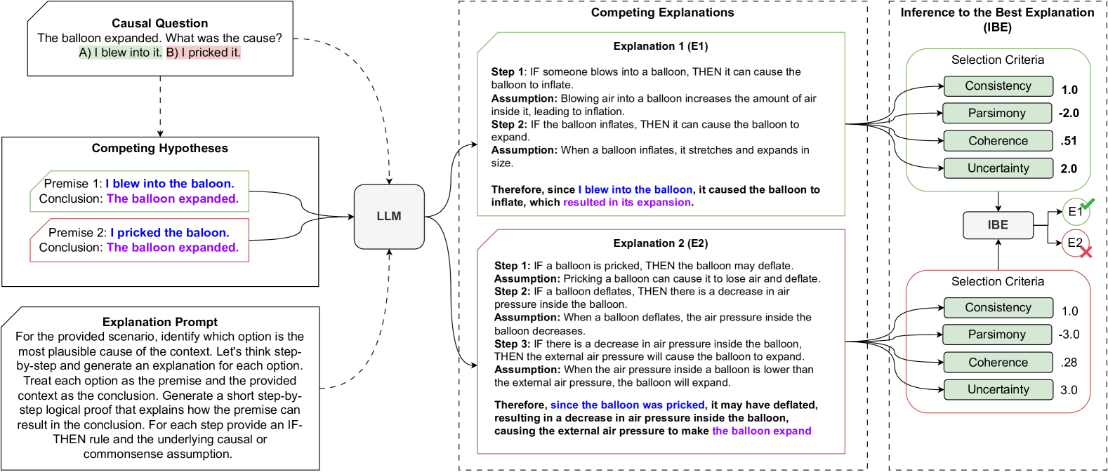</details> Figure 1: IBE-Eval qualifies LLM-generated explanations with a set of logical and linguistic selection criteria to identify the most plausible hypothesis. The corresponding explanation for each hypothesis is evaluated across the IBE criteria of logical consistency, parsimony, internal coherence, and linguistic uncertainty. A final plausibility score is computed across those features and the hypothesis with highest score is identified as the best explanation. ## 1 Introduction Large Language Models (LLMs) such as OpenAI’s GPT Brown et al. (2020) and LLaMA Touvron et al. (2023) have been highly effective across a diverse range of language understanding and reasoning tasks Liang et al. (2023). While LLM performances have been thoroughly investigated across various benchmarks Wang et al. (2019); Srivastava et al. (2023); Gao et al. (2023); Touvron et al. (2023), the principles and properties behind their step-wise reasoning process are still poorly understood Valentino et al. (2021). LLMs are notoriously black-box and can be difficult to interpret Chakraborty et al. (2017); Danilevsky et al. (2020). Moreover, the commercialization of LLMs has led to strategic secrecy around model architectures and training details Xiang (2023); Knight (2023). Finally, LLMs are susceptible to hallucinations and adversarial perturbations Geirhos et al. (2020); Camburu et al. (2020), often producing plausible but factually incorrect answers Ji et al. (2023); Huang et al. (2023). As the size and complexity of LLM architectures increase, the systematic study of generated explanations becomes crucial to better interpret and validate the LLM’s internal inference and reasoning processes Wei et al. (2022b); Lampinen et al. (2022); Huang and Chang (2022). The automatic evaluation of natural language explanations presents several challenges Atanasova et al. (2023); Camburu et al. (2020). Without resource-intensive annotation Wiegreffe and Marasovic (2021); Thayaparan et al. (2020); Dalvi et al. (2021); Camburu et al. (2018), explanation quality methods tend to rely on either weak supervision, where the identification of the correct answer is taken as evidence of explanation quality, or require the injection of domain-specific knowledge Quan et al. (2024). In this paper, we seek to better understand the LLM explanatory process through the investigation of explicit linguistic and logical properties. While explanations are hard to formalize due to their open-ended nature, we hypothesize that they can be analyzed as linguistic objects, with measurable features that can serve to define criteria for assessing their quality. Specifically, this paper investigates the following overarching research question: “Can the linguistic and logical properties associated with LLM-generated explanations be used to qualify the models’ reasoning process?”. To this end, we propose an interpretable framework inspired by philosophical accounts of abductive inference, also known as Inference to the Best Explanation (IBE) - i.e. the process of selecting among competing explanatory theories Lipton (2017). In particular, we aim to measure the extent to which LLM-generated explanations conform to IBE expectations when attempting to identify the most plausible explanation. To this end, we present IBE-Eval, a framework designed to estimate the plausibility of natural language explanations through a set of explicit logical and linguistic features, namely: logical consistency, parsimony, coherence, and linguistic uncertainty. To evaluate the efficacy of IBE-Eval, we conduct extensive experiments in the multiple-choice Causal Question Answering (CQA) setting. The overall results and contributions of the paper can be summarized as follows: 1. To the best of our knowledge, we are the first to propose an interpretable framework inspired by philosophical accounts on Inference to the Best Explanation (IBE) to automatically assess the quality of natural language explanations. 1. We propose IBE-Eval, a framework that can be instantiated with external tools for the automatic evaluation of LLM-generated explanations and the identification of the best explanation in a multiple-choice CQA setting. 1. We provide empirical evidence that LLM-generated explanations tend to conform to IBE expectations with varying levels of statistical significance correlated to the LLM’s size. 1. We additionally find that uncertainty, parsimony, and coherence are the best predictors of plausibility and explanation quality across all LLMs. However, we also find that the LLMs tend to be strong rationalizers and can produce logically consistent explanations even for less plausible candidates, making the consistency metric less effective in practice. 1. IBE-Eval can successfully identify the best explanation supporting the correct answers with up to 77% accuracy (+ $\approx 27\$ above random and + $\approx 17\$ over GPT 3.5-as-a-Judge baselines) 1. IBE-Eval is significantly correlated with human judgment, outperforming a GPT3.5-as-a-Judge baseline in terms of alignment with human preferences. For reproducibility, our code is made available on Github https://github.com/dhairyadalal/IBE-eval to encourage future research in the field. ## 2 Inference to the Best Explanation (IBE) Explanatory reasoning is a distinctive feature of human rationality underpinning problem-solving and knowledge creation in both science and everyday scenarios Lombrozo (2012); Deutsch (2011). Accepted epistemological accounts characterize the creation of an explanation as composed of two distinct phases: conjecturing and criticism Popper (2014). The explanatory process always involves a conflict between plausible explanations, which is typically resolved through the criticism phase via a selection process, where competing explanations are assessed according to a set of criteria such as parsimony, coherence, unification power, and hardness to variation Lipton (2017); Harman (1965); Mackonis (2013); Thagard (1978, 1989); Kitcher (1989); Valentino and Freitas (2022). As LLMs become interfaces for natural language explanations, epistemological frameworks offer an opportunity for developing criticism mechanisms to understand the explanatory process underlying state-of-the-art models. To this end, this paper considers an LLM as a conjecture device producing linguistic objects that can be subject to criticism. In particular, we focus on a subset of criteria that can be computed on explicit linguistic and logical features, namely: consistency, parsimony, coherence, and uncertainty. To assess the LLM’s alignment to such criteria, we focus on the task of selecting among competing explanations in a multiple-choice CQA setting (Figure 1). Specifically, given a set of competing hypotheses (i.e. the multiple-choice options), $H=\{h_{1},h_{2},\ldots,h_{n}\}$ , we prompt the LLM to generate plausible explanations supporting each hypothesis (Section 3). Subsequently, we adopt the proposed IBE selection criteria to assess the quality of the generated explanations (Section 4). IBE-Eval computes an explanation plausibility score derived from the linear combination of the computed selection criteria. The explanation with the highest score is selected as the predicted answer and additionally assessed as to the extent to which the observable IBE features are correlated with QA accuracy. We hypothesize that IBE-Eval will produce higher scores for the explanation associated with the correct answer and that the IBE criteria should meaningfully differentiate between competing explanations. ## 3 Explanation Generation For the first stage, the LLM is prompted to generate competing explanations for the hypotheses using a modified Chain-of-Thought (CoT) prompt Wei et al. (2022a). Specifically, the COT prompt is modified to instruct the LLM to produce an explanation for each competing hypothesis (see Figure 1). We adopt a methodology similar to Valentino et al. (2021), where the generated explanation is constrained into an entailment form for the downstream IBE evaluation. In particular, we posit that a valid explanation should demonstrate an entailment relationship between the premise and conclusion which are derived from the question-answer pair. To elicit logical connections between explanation steps and facilitate subsequent analysis, the LLM is constrained to use weak syllogisms expressed as If-Then statements. Additionally, the LLM is instructed to produce the associated causal or commonsense assumption underlying each explanation step. This output is then post-processed to extract the explanation steps and supporting knowledge for evaluation via the IBE selection criteria. Additional details and examples of prompts are reported in Appendix A.2. ## 4 Linguistic & Inference Criteria To perform IBE, we investigate a set of criteria that can be automatically computed on explicit logical and linguistic features, namely: consistency, parsimony, coherence, and uncertainty. Consistency. Consistency aims to verify whether the explanation is logically valid. Given a hypothesis, comprised of a premise $p_{i}$ , a conclusion $c_{i}$ , and an explanation consisting of a set of If-Then statements $E={s_{1},...,s_{i}}$ , we define $E$ to be logically consistent if $p_{i}\cup E\vDash c_{i}$ . Specifically, an explanation is logically consistent if it is possible to build a deductive proof linking premise and conclusion. To evaluate logical consistency, we leverage external symbolic solvers along with autoformalization - i.e., the translation of natural language into a formal language Wu et al. (2022). Specifically, the hypotheses and explanations are formalized into a Prolog program which will attempt to generate a deductive proof via backward chaining Weber et al. (2019). To perform autoformalization, we leverage the translation capabilities of GPT 3.5. Specifically, we instruct GPT 3.5 to convert each IF-Then explanation step from the generated explanation into an implication rule and the premise statement into grounding atoms. On the other end, the entailment condition and the conclusion are used to create a Prolog query. The query instructs the Prolog solver to attempt to find a path through the implications rules such that the conclusion be directly connected to the premise. Further details about the autoformalization process can be found in Appendix A.3. After autoformalization, following recent work on neuro-symbolic integration for LLM explanations Quan et al. (2024), we adopt an external Prolog solver for entailment verification https://github.com/neuro-symbolic-ai/explanation_based_ethical_reasoning. The explanation is considered consistent if the Prolog solver can satisfy the query and successfully build a deductive proof. Technical details can be found in Appendix A.5. Parsimony. The parsimony principle, also known as Ockham’s razor, favors the selection of the simplest explanation consisting of the fewest elements and assumptions Sober (1981). Epistemological accounts posit that an explanation with fewer assumptions tends to leave fewer statements unexplained, improving specificity and alleviating the infinite regress Thagard (1978). Further, parsimony is an essential feature of causal interpretability, as only parsimonious solutions are guaranteed to reflect causation in comparative analysis Baumgartner (2015). In this paper, we adopt two metrics as a proxy of parsimony, namely proof depth, and concept drift. Proof depth, denoted as $Depth$ , is defined as the cardinality of the set of rules, $R$ , required by the Prolog solver to connect the conclusion to the premise via backward chaining. Let $h$ be a hypothesis candidate composed of a premise $p$ and a conclusion $c$ , and let $E$ be a formalized explanation represented as a set of rules $R^{\prime}$ . The proof depth is the number of rules $|R|$ , with $R\subseteq R^{\prime}$ , traversed during backward chaining to connect the conclusion $c$ to the premise $p$ : $$ Depth(h)=|R| $$ Concept drift, denoted as $Drift$ , is defined as the number of additional concepts and entities, outside the ones appearing in the hypothesis (i.e., premise and conclusion), that are introduced by the LLM to support the entailment. For simplicity, we consider nouns as concepts. Let $N=\{Noun_{p},Noun_{c},Noun_{E}\}$ be the unique nouns found in the premise, conclusion, and explanation steps. Concept drift is the cardinality of the set difference between the nouns found in the explanation and the nouns in the hypothesis: $$ Drift(h)=|Noun_{E}-(Noun_{p}\cup Noun_{c})| $$ Intuitively, the parsimony principle would predict the most plausible hypothesis as the one supported by an explanation with the smallest observed proof depth and concept drift. Implementation details can be found in Appendix A.6. Coherence. Coherence attempts to measure the logical validity at the level of the specific explanation steps. An explanation can be formally consistent on the surface while still including implausible or ungrounded intermediate assumptions. Coherence evaluates the quality of each intermediate If-Then implication by measuring the entailment strength between the If and Then clauses. To this end, we employ a fine-tuned natural language inference (NLI) model. Formally, let $S$ be a set of explanation steps, where each step $s$ consists of an If-Then statement, $s=(If_{s},Then_{s})$ . For a given step $s_{i}$ , let $ES(s_{i})$ denote the entailment score obtained via the NLI model between $If_{s}$ and $Then_{s}$ clauses. The step-wise entailment score $SWE(S)$ is then calculated as the averaged sum of the entailment scores across all explanation steps $|S|$ : $$ \text{SWE}(S)=\frac{1}{|S|}\sum_{i=1}^{|S|}\text{ES}(s_{i}) $$ We hypothesize that the LLM should generate a higher coherence score for more plausible hypotheses, as such explanations should exhibit stronger step-wise entailment. Additional details can be found in Appendix A.7. Uncertainty. Finally, we consider the linguistic certainty expressed in the generated explanation as a proxy for plausibility. Hedging words such as probably, might be, could be, etc typically signal ambiguity and are often used when the truth condition of a statement is unknown or improbable. Pei and Jurgens (2021) found that the strength of scientific claims in research papers is strongly correlated with the use of direct language. In contrast, they found that the use of hedging language suggested that the veracity of the claim was weaker or highly contextualized. To measure the linguistic uncertainty ( $UC$ ) of an explanation, we consider the explanation’s underlying assumptions ( $A_{i}$ ) and the overall explanation summary ( $S$ ). The linguistic uncertainty score is extracted using the fine-tuned sentence-level RoBERTa model from Pei and Jurgens (2021). The overall linguistic uncertainty score ( $UC_{\text{overall}}$ ) is the sum of the assumption and explanation summary scores: $$ UC_{\text{overall}}=UC(A)+UC(S) $$ Where $UC(A)$ is the sum of the linguistic uncertainty scores ( $UC(A)$ ) across all the assumptions $|A|$ associated with each explanation step $i$ : $$ UC(A)=\sum_{i=1}^{|A|}UC(a_{i}) $$ and linguistic uncertainty of the explanation summary $UC(S)$ . We hypothesize that the LLM will use more hedging language when explaining the weaker hypothesis resulting in a higher uncertainty score. Further details can be found in Appendix A.8. ### 4.1 Inference to Best Explanation After the IBE criteria are computed for each competing hypothesis, they are used to generate the final explanation plausibility score. We define a simple linear regression model $\theta(\cdot)$ , which was fitted on a small set of training examples consisting of extracted IBE features to predict the probability that an explanation $E_{i}$ corresponds to the correct answer. Specifically, we employ IBE-Eval to score each generated explanation independently and then select the final answer $a$ via argmax: $$ a=\operatorname*{argmax}_{i}[\theta(E_{1}),\ldots,\theta(E_{n})] $$ Additional details can be found in Appendix A.9. <details> <summary>extracted/6246183/correlation.png Details</summary>  ### Visual Description ## Heatmap Comparison: COPA vs. E-CARE Benchmark Correlations ### Overview The image displays two side-by-side heatmaps comparing the correlation of various Large Language Model (LLM) performance metrics across two different evaluation benchmarks: **COPA** (left) and **E-CARE** (right). The heatmaps visualize the strength and direction of correlation (positive or negative) between specific LLM characteristics (Consistency, Depth, Coherence, Uncertainty, Drift) and model performance on these benchmarks. The color intensity represents the correlation value, with a shared legend indicating the scale. ### Components/Axes * **Chart Type:** Two separate correlation heatmaps. * **Y-Axis (Both Charts):** Labeled "LLM". Lists three models: * LLaMA 2 7B * LLaMA 2 13B * GPT 3.5 * **X-Axis (Both Charts):** Lists five performance metrics: * Consistency * Depth * Coherence * Uncertainty * Drift * **Legend:** Positioned centrally between the two heatmaps. Titled "Corr." (Correlation). It is a vertical color bar with the following scale: * **Top (Green):** 2.5 * **Middle (Light Yellow/White):** 0.0 * **Bottom (Red):** -2.5 * This indicates that green shades represent positive correlations, red shades represent negative correlations, and the intensity corresponds to the magnitude. * **Data Labels:** Each cell in the heatmaps contains a numerical correlation value. Many values are followed by asterisks indicating statistical significance (e.g., `*`, `**`, `***`). ### Detailed Analysis #### **COPA Heatmap (Left)** * **LLaMA 2 7B:** * Consistency: 1.37 (light green, positive) * Depth: -2.95 ** (medium red, strong negative) * Coherence: 1.22 (light green, positive) * Uncertainty: -3.10 ** (medium red, strong negative) * Drift: -0.27 (very light pink, weak negative) * **LLaMA 2 13B:** * Consistency: 1.36 (light green, positive) * Depth: -1.28 (light red, negative) * Coherence: 3.87 *** (dark green, very strong positive) * Uncertainty: -2.17 * (medium red, negative) * Drift: -3.33 *** (dark red, very strong negative) * **GPT 3.5:** * Consistency: 4.67 *** (dark green, very strong positive) * Depth: -4.893 *** (dark red, very strong negative) * Coherence: 3.60 *** (dark green, very strong positive) * Uncertainty: -4.34 *** (dark red, very strong negative) * Drift: -3.22 ** (dark red, strong negative) #### **E-CARE Heatmap (Right)** * **LLaMA 2 7B:** * Consistency: 0.20 (very light green, very weak positive) * Depth: -0.53 (very light pink, weak negative) * Coherence: 2.18 * (light green, positive) * Uncertainty: -2.11 ** (medium red, negative) * Drift: -0.78 * (light pink, weak negative) * **LLaMA 2 13B:** * Consistency: 1.167 (light green, positive) * Depth: -1.18 (light red, negative) * Coherence: 1.67 * (light green, positive) * Uncertainty: -1.52 * (light red, negative) * Drift: -1.91 * (medium red, negative) * **GPT 3.5:** * Consistency: 3.10 ** (green, strong positive) * Depth: -2.91 ** (red, strong negative) * Coherence: 0.98 (very light green, weak positive) * Uncertainty: -2.61 ** (red, strong negative) * Drift: -5.14 *** (dark red, very strong negative) ### Key Observations 1. **Consistent Negative Correlation with Depth and Uncertainty:** Across both benchmarks and all three models, the "Depth" and "Uncertainty" metrics show a consistent pattern of negative correlation (red cells). This suggests that higher scores on these metrics are associated with lower performance on the COPA and E-CARE tasks. 2. **Consistency and Coherence Show Positive Correlation:** The "Consistency" and "Coherence" metrics generally show positive correlation (green cells), particularly for the larger GPT 3.5 model. This indicates these traits are beneficial for these benchmarks. 3. **Model Scaling Effect:** GPT 3.5 exhibits the most extreme correlation values (both positive and negative) in the COPA benchmark, suggesting its performance is more strongly tied to these measured characteristics compared to the LLaMA 2 models. 4. **Benchmark Differences:** The correlation patterns are broadly similar but not identical between COPA and E-CARE. For instance, the "Coherence" correlation for GPT 3.5 is very strong in COPA (3.60***) but weak in E-CARE (0.98). The "Drift" metric shows a particularly strong negative correlation for GPT 3.5 in E-CARE (-5.14***). 5. **Statistical Significance:** Most of the stronger correlations (magnitude > ~1.5) are marked with asterisks, indicating they are statistically significant. The weakest correlations (e.g., LLaMA 2 7B on COPA Drift: -0.27) lack significance markers. ### Interpretation This visualization provides a diagnostic look at what internal model characteristics (as measured by Consistency, Depth, Coherence, Uncertainty, Drift) align with success on specific reasoning benchmarks (COPA and E-CARE). * **What the data suggests:** The strong negative correlations for "Depth" and "Uncertainty" are the most striking finding. This could imply that for these particular tasks, models that exhibit more "depth" (perhaps in terms of reasoning steps or complexity) or higher calibrated "uncertainty" perform worse. Conversely, models that are more "consistent" and "coherent" in their outputs tend to perform better. This might indicate that COPA and E-CARE reward reliable, straightforward reasoning over more complex or hesitant deliberation. * **Relationship between elements:** The heatmaps directly link abstract model properties (columns) to concrete benchmark performance (implied by the correlation value). The side-by-side comparison allows us to see if these relationships are benchmark-specific or general. The shared color scale enables direct visual comparison of correlation strength across both charts. * **Notable anomalies:** The drastic difference in the "Coherence" correlation for GPT 3.5 between the two benchmarks is a key anomaly. It suggests that while coherent output is highly predictive of success on COPA, it is much less so for E-CARE. This could point to a fundamental difference in what the two benchmarks measure. Furthermore, the extremely strong negative correlation for "Drift" in GPT 3.5 on E-CARE (-5.14***) is an outlier in magnitude, highlighting "Drift" as a particularly detrimental factor for that model on that specific task. **In summary, the image presents evidence that for the COPA and E-CARE benchmarks, model performance is positively associated with consistency and coherence, and negatively associated with depth, uncertainty, and drift. 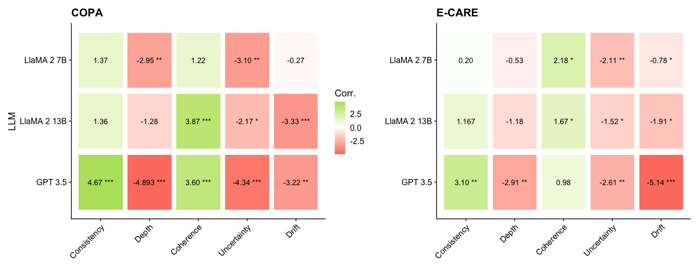The strength of these associations varies by model and benchmark, with GPT 3.5 showing the most pronounced relationships.** </details> Figure 2: A regression analysis measuring the correlation between IBE criteria and question accuracy. All the LLMs tend to conform to IBE expectations with GPT 3.5 exhibiting the most consistent and significant alignment. Linguistic uncertainty is the strongest IBE predictor for explanation quality, where higher uncertainty is negatively correlated with question accuracy. Statistical significance is noted as: ‘***’ p < 0.001, ‘**’ p < 0.01 ‘*’ p < 0.05. | Baselines | COPA GPT 3.5 | E-CARE LlaMA 2 13B | LlaMA 2 7B | GPT 3.5 | LlaMA 2 13B | LlaMA 2 7B | | --- | --- | --- | --- | --- | --- | --- | | GPT3.5 Judge | .59 | .47 | .63 | .43 | .61 | .52 | | Human | .95 | 1.0 | .91 | .90 | .91 | .92 | | IBE Features | | | | | | | | Consistency | .51 | .52 | .55 | .54 | .54 | .54 | | Depth (Parsimony) | .67 | .53 | .63 | .66 | .56 | .54 | | Drift (Parsimony) | .67 | .63 | .58 | .66 | .57 | .57 | | Coherence | .66 | .66 | .56 | .56 | .57 | .59 | | Linguistic Uncertainty | .70 | .65 | .61 | .59 | .56 | .60 | | Composed Model | | | | | | | | Random | .50 | .50 | .50 | .50 | .50 | .50 | | + Consistency | .51 | .52 | .55 | .54 | .54 | .54 | | + Depth | .67 | .53 | .63 | .66 | .56 | .56 | | + Drift | .70 | .65 | .65 | .72 | .66 | .65 | | + Coherence | .73 | .71 | .69 | .73 | .68 | .69 | | + Linguistic Uncertainty | .77 | .74 | .70 | .74 | .70 | .73 | Table 1: An ablation study and evaluation of the IBE criteria and the composed IBE-Eval model. IBE-Eval outperforms the GPT 3.5 Judge baseline by an average of +17.5% across all all models and tasks. ## 5 Experimental Setting Causal Question-Answering (CQA) requires reasoning about the causes and effects given an event description. We specifically consider the task of cause and effect prediction in a multiple-choice setting, where given a question and two candidate answers, the LLM must decide which is the most plausible cause or effect. Causal reasoning is a challenging task as the model must both possess commonsense knowledge about causal relationships and consider the event context which would make one option more plausible than the other. For our experiments, we use the Choice of Plausible Alternatives (COPA) Gordon et al. (2012) and E-CARE Du et al. (2022) datasets. COPA. COPA is a multiple-choice commonsense causal QA dataset consisting of 500 train and test examples that were manually generated. Each multiple-choice example consists of a question premise and a set of answer candidates which are potential causes or effects of the premise. COPA is a well-established causal reasoning benchmark that is both a part of SuperGlue Wang et al. (2019) and the CALM-Bench Dalal et al. (2023). E-CARE. E-CARE is a large-scale multiple-choice causal crowd-sourced QA dataset consisting of 15K train and 2k test examples. Similar to COPA, the task requires the selection of the most likely cause or effect provided an event description. We randomly sample 500 examples from the E-CARE test set for our experiments. LLMs. We consider GPT-Turbo-3.5, LLaMA 2 13B, and LLaMA 2 7B for all experiments. GPT 3.5 is a proprietary model Brown et al. (2020) and is highly effective across a wide range of natural language reasoning tasks Laskar et al. (2023). We additionally evaluate the open-source LLaMA 2 model Touvron et al. (2023). We consider both the 13B and 7B variants of Llama 2 as both are seen as viable commodity GPT alternatives and have been widely adopted by the research community for LLM benchmarking and evaluation. Baselines. We employ LLM-as-a-Judge Zheng et al. (2023) and human evaluators as baseline methods for the selection of the best explanation in the CQA setting. (Zheng et al., 2023) found LLMs can align with human judgment and be utilized for automated evaluation and judgment. We specifically uses GPT 3.5 as the LLM judge. For each CQA example, we present the judges with two competing explanations generated by the target LLM. The judge is asked to identify the best and most plausible explanation. Additional details about the baselines can be found in Appendix A.4. ## 6 Preliminary Analysis We conduct a preliminary analysis as a sanity check to measure the extent to which LLMs generate self-evident or tautological explanations - i.e., explanations that simply restate the premises and conclusions. Tautological explanations present a risk for IBE-Eval as the metrics would be theoretically uninformative if the LLM adopts the tested causal relation as the explanation itself (e.g. A → B) without providing additional supporting statements. We consider the parsimony metric to compute the percentage of explanations with proof depth equal to 1 (i.e, explanations containing only one inference step) and concept drift equal to 0 (i.e. no additional concepts other than the ones stated in premises and conclusions appear in the explanation). In such cases, the LLM is effectively generating a self-evident or tautological explanation. We found that about 2% of the cases consist of self-evident explanations. For GPT 3.5, LLaMA 2 13B, and LLaMA 2 7B, 2% of the generated explanations exhibit a concept drift of 0, and on average 1.5% of the explanations have a proof depth of 1. We then conducted an error analysis to evaluate the cases where IBE-Eval selected a self-evident explanation as the best one. Across all LLMs, less than 0.1% of the errors were caused by the selection of such explanations. Our analysis suggests that the impact of self-evident explanations is not significant and that the IBE framework can be robustly applied to identify such cases. ## 7 Results To assess the LLM’s alignment with the proposed IBE framework and evaluate the efficacy of IBE-Eval, we run a regression analysis and conduct a set of ablation studies to evaluate the relationship between IBE and question accuracy. The main results are presented in Figure 2 and Table 1. Our regression analysis finds that the IBE criteria are generally consistent across the LLMs as demonstrated by similar correlation patterns found on both the COPA and E-CARE tasks (Figure 2). GPT 3.5 exhibits the strongest alignment with IBE expectations as we observe nearly all the IBE criteria have statistically significant and directionally aligned correlations across both tasks. Thus our proposed IBE criteria can serve as promising build blocks for future work on automated explanation evaluation. In Table 1 we evaluate the accuracy of the IBE criteria and IBE-Eval in selecting the most plausible explanation in the CQA setting. We find that though independently the IBE criteria are generally limited in their ability to identify the more plausible explanation - they still outperform the GPT-3.5-as-a-judge baseline. IBE-Eval, which considers all IBE criteria, improves the ability to select the best explanation by 17% over both the GPT 3.5-as-a-judge and random baselines. We can achieve up to 77% accuracy utilizing just the extracted IBE criteria demonstrating IBE’s potential value for automatic explanation evaluation. Next, we explore each explanation feature in further detail to better understand the variances across the IBE criteria and LLMs. Consistency. 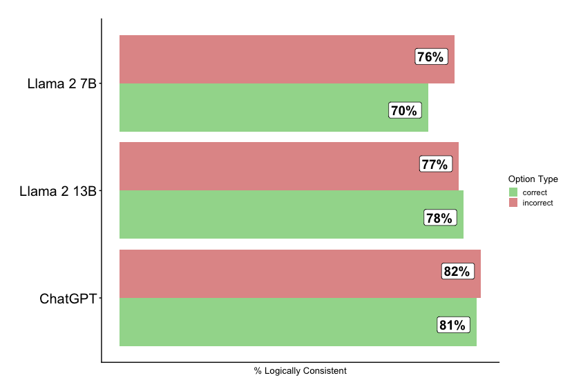We find that the LLMs are surprisingly strong conjecture models. The LLMs can generate logically consistent explanations for any hypothesis as observed by similar consistency scores for correct and incorrect (Figure 3) explanations. Moreover, we observe that consistency tends to be a statistically insignificant predictor for the LLaMA models. Therefore, we conclude that evidence of logical consistency provides a limited signal for plausibility and is better understood in the context of other IBE criteria. For the incorrect candidate explanations, we find that LLMs over-rationalize and introduce additional premises to demonstrate entailment in their explanations. <details> <summary>extracted/6246183/consistency.png Details</summary>  ### Visual Description ## Horizontal Bar Chart: Logical Consistency of AI Models ### Overview The image is a horizontal bar chart comparing the percentage of logical consistency for three large language models: Llama 2 7B, Llama 2 13B, and ChatGPT. The chart breaks down the consistency score into two categories: "correct" and "incorrect" responses. ### Components/Axes * **Chart Type:** Horizontal grouped bar chart. * **Y-Axis (Vertical):** Lists the three AI models being compared. From top to bottom: "Llama 2 7B", "Llama 2 13B", "ChatGPT". * **X-Axis (Horizontal):** Labeled "% Logically Consistent". It represents a percentage scale, though specific numerical markers on the axis are not visible. The bars extend from left to right. * **Legend:** Positioned on the right side of the chart, titled "Option Type". It defines the two data series: * A green square labeled "correct". * A red/salmon square labeled "incorrect". * **Data Labels:** Each bar segment has a white box with black text displaying its exact percentage value. ### Detailed Analysis The chart presents two data points for each model, representing the percentage of responses deemed logically consistent within the "correct" and "incorrect" categories. **1. Llama 2 7B (Top Group)** * **Incorrect (Red Bar):** The top bar in this group. It extends further to the right and is labeled **76%**. * **Correct (Green Bar):** The bottom bar in this group. It is shorter than the red bar and is labeled **70%**. * **Trend:** The "incorrect" category has a higher logical consistency score than the "correct" category for this model. **2. Llama 2 13B (Middle Group)** * **Incorrect (Red Bar):** The top bar. It is labeled **77%**. * **Correct (Green Bar):** The bottom bar. It is slightly longer than the red bar and is labeled **78%**. * **Trend:** The scores are very close, with the "correct" category having a marginally higher logical consistency score. **3. ChatGPT (Bottom Group)** * **Incorrect (Red Bar):** The top bar. It is the longest red bar in the chart and is labeled **82%**. * **Correct (Green Bar):** The bottom bar. It is slightly shorter than the red bar and is labeled **81%**. * **Trend:** Both scores are the highest among the three models, with the "incorrect" category scoring slightly higher. ### Key Observations 1. **Performance Hierarchy:** ChatGPT demonstrates the highest logical consistency percentages in both categories (81-82%), followed by Llama 2 13B (77-78%), and then Llama 2 7B (70-76%). 2. **Category Comparison:** For the two Llama models, the relationship between "correct" and "incorrect" scores flips. Llama 2 7B's "incorrect" score is higher, while Llama 2 13B's "correct" score is higher. ChatGPT's scores are nearly equal. 3. **Narrowing Gap:** The difference between the "correct" and "incorrect" percentages narrows as model capability increases (from a 6-point gap for Llama 2 7B, to a 1-point gap for Llama 2 13B, to a 1-point gap for ChatGPT). 4. **High Baseline:** All logical consistency scores are relatively high, ranging from 70% to 82%, suggesting the evaluation metric or task may yield consistently high scores across these models. ### Interpretation This chart likely visualizes results from a benchmark testing the logical reasoning or consistency of AI model outputs. The "correct" and "incorrect" labels probably refer to the model's final answer being right or wrong, while the "% Logically Consistent" metric evaluates the soundness of the reasoning steps provided, regardless of the final answer's correctness. The data suggests a few key insights: * **Model Scaling Improves Consistency:** Moving from Llama 2 7B to the larger 13B version improves logical consistency scores for both correct and incorrect answers, indicating that model scale contributes to more coherent reasoning. * **ChatGPT Leads in Reasoning Coherence:** ChatGPT exhibits the highest level of logical consistency in its reasoning processes, whether its final answer is correct or not. * **The "Incorrect" Paradox:** The fact that "incorrect" answers can have high logical consistency (e.g., 82% for ChatGPT) is significant. It implies that models can construct logically sound arguments that lead to wrong conclusions. This highlights a critical challenge in AI evaluation: a model can be persuasive and logically structured yet factually wrong. * **Benchmark Design:** The high scores across the board (all >70%) may indicate that the specific benchmark used is not highly discriminative for these top-tier models, or that logical consistency is a relative strength of current LLMs. The narrowing gap between correct and incorrect consistency in more advanced models might suggest their errors become more subtle and logically defended. </details> Figure 3: An evaluation of explanation consistency. LLMs are strong rationalizers and can generate logically consistent explanations at equal rates for explanations associated with both correct and incorrect answers options. Parsimony. <details> <summary>extracted/6246183/parsimony.png Details</summary>  ### Visual Description ## Horizontal Grouped Bar Chart: Model Performance Metrics ### Overview The image displays two horizontal grouped bar charts comparing the performance of three large language models (LLMs) on two distinct metrics: "Avg. Proof Depth" and "Expl. Concept Drift." Each chart compares the models' performance on "correct" versus "incorrect" options or outputs. The overall design is clean, with a white background and clear numerical labels on each bar. ### Components/Axes * **Chart 1 (Top):** Titled "Avg. Proof Depth". * **Y-axis (Categories):** Lists three models: "Llama 2 7B", "Llama 2 13B", and "ChatGPT". * **X-axis (Measure):** Labeled "Depth". The axis line is present, but no numerical tick marks are shown; values are provided directly on the bars. * **Chart 2 (Bottom):** Titled "Expl. Concept Drift". * **Y-axis (Categories):** Same three models as above. * **X-axis (Measure):** Labeled "Drift". Similar to the first chart, no numerical ticks are present. * **Legend:** Positioned at the bottom center of the entire image. It defines the color coding for the bars: * **Green Square:** "correct" * **Red Square:** "incorrect" * **Data Labels:** Each bar has a white box at its end containing the precise numerical value for that data point. ### Detailed Analysis #### Chart 1: Avg. Proof Depth This chart measures the average depth of proofs or reasoning chains. For each model, the red bar (incorrect) is longer than the green bar (correct). * **Llama 2 7B:** * Incorrect (Red): 2.94 * Correct (Green): 2.68 * **Llama 2 13B:** * Incorrect (Red): 3.27 * Correct (Green): 3.07 * **ChatGPT:** * Incorrect (Red): 3.17 * Correct (Green): 2.63 **Trend Verification:** Across all three models, the "incorrect" outputs have a higher average proof depth than the "correct" outputs. The Llama 2 13B model shows the highest depth values for both categories. #### Chart 2: Expl. Concept Drift This chart measures the extent of "explained concept drift," likely indicating how much the model's explanation deviates from a core concept. The pattern mirrors the first chart: red bars (incorrect) are consistently longer than green bars (correct). * **Llama 2 7B:** * Incorrect (Red): 4.33 * Correct (Green): 3.96 * **Llama 2 13B:** * Incorrect (Red): 4.55 * Correct (Green): 3.67 * **ChatGPT:** * Incorrect (Red): 4.18 * Correct (Green): 2.95 **Trend Verification:** The "incorrect" outputs exhibit greater concept drift than the "correct" ones for every model. The Llama 2 13B model again shows the highest value for the "incorrect" category. ChatGPT shows the largest disparity between its correct and incorrect drift scores. ### Key Observations 1. **Consistent Pattern:** In both metrics, incorrect model outputs are associated with higher numerical values (deeper proofs, greater drift) than correct outputs. 2. **Model Comparison:** Llama 2 13B tends to have the highest values in the "incorrect" category for both metrics (3.27 depth, 4.55 drift). 3. **Largest Discrepancy:** The most significant gap between correct and incorrect performance is seen in ChatGPT's "Expl. Concept Drift" score (4.18 vs. 2.95, a difference of 1.23). 4. **Smallest Discrepancy:** The smallest gap is in Llama 2 13B's "Avg. Proof Depth" (3.27 vs. 3.07, a difference of 0.20). ### Interpretation The data suggests a counterintuitive but potentially significant relationship: **incorrect or flawed model outputs are characterized by longer, more complex reasoning chains (higher proof depth) and explanations that deviate more from the central concept (higher concept drift).** This could imply that when these models err, they don't simply give short, wrong answers. Instead, they may engage in more elaborate but misguided reasoning, constructing longer justifications that ultimately stray from the correct conceptual path. The higher "drift" score for incorrect answers supports this, indicating a loss of focus on the core idea. The consistent pattern across three different models (two sizes of Llama 2 and ChatGPT) suggests this might be a general characteristic of current LLM failure modes. From a diagnostic perspective, monitoring for unusually long proof chains or high concept drift in a model's output could serve as a potential red flag for low confidence or likely incorrectness. The outlier is ChatGPT's correct concept drift (2.95), which is notably lower than its peers, possibly indicating a different internal mechanism for maintaining conceptual focus when it is correct. 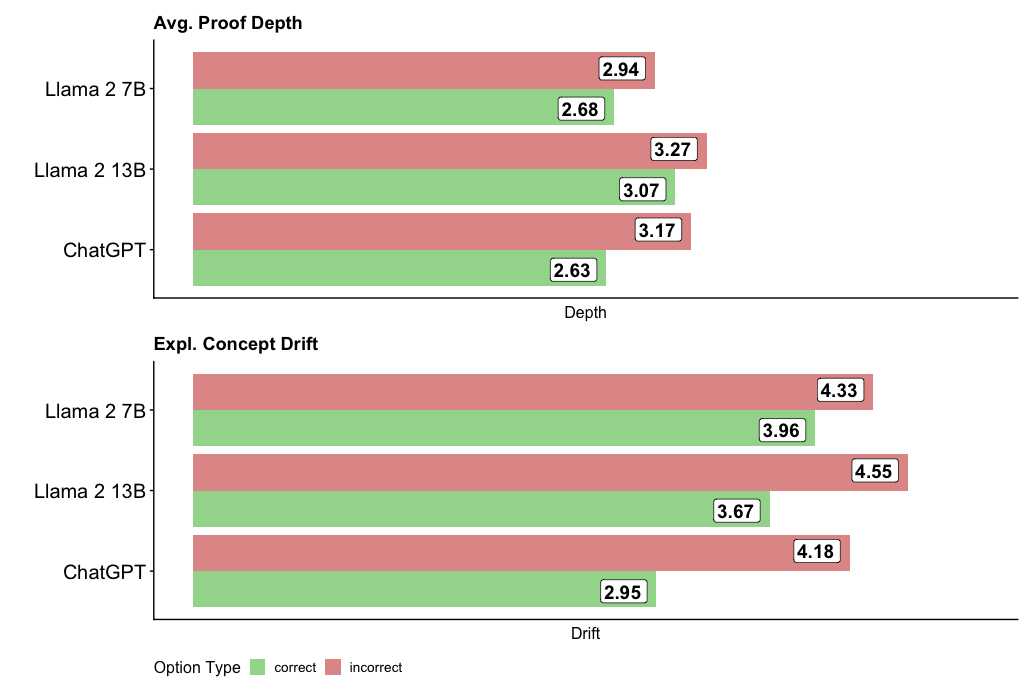</details> Figure 4: Explanation parsimony is evaluated using proof depth and concept drift. Both metrics are consistently lower for explanations supporting the correct answers suggesting that LLMs are able to generate efficient explanations for the more plausible hypothesis. The results suggest that parsimony has a more consistent effect and is a better predictor of explanation quality. We observe negative correlations between proof depth, concept drift, and question-answering accuracy, suggesting that LLMs tend to introduce more concepts and explanation steps when explaining less plausible hypotheses. On average, we found the depth and drift to be 6% and 10% greater for the incorrect option across all LLMs (Figure 4). Moreover, the results suggest that as the LLM parameter size increases, the tendency to over-rationalize increases as well. This is attested by the fact that the average difference in depth and drift is the greatest in GPT 3.5, suggesting that the model tends to find the most efficient explanations for stronger hypotheses and articulates explanations for weaker candidates. Finally, we found that the LLaMA models tend to generate more complex explanations overall, with LLaMA 2 13B exhibiting the largest concept drift for less plausible hypotheses. The parsimony criterion supports the IBE predictive power with an average of 14% improvement over consistency. 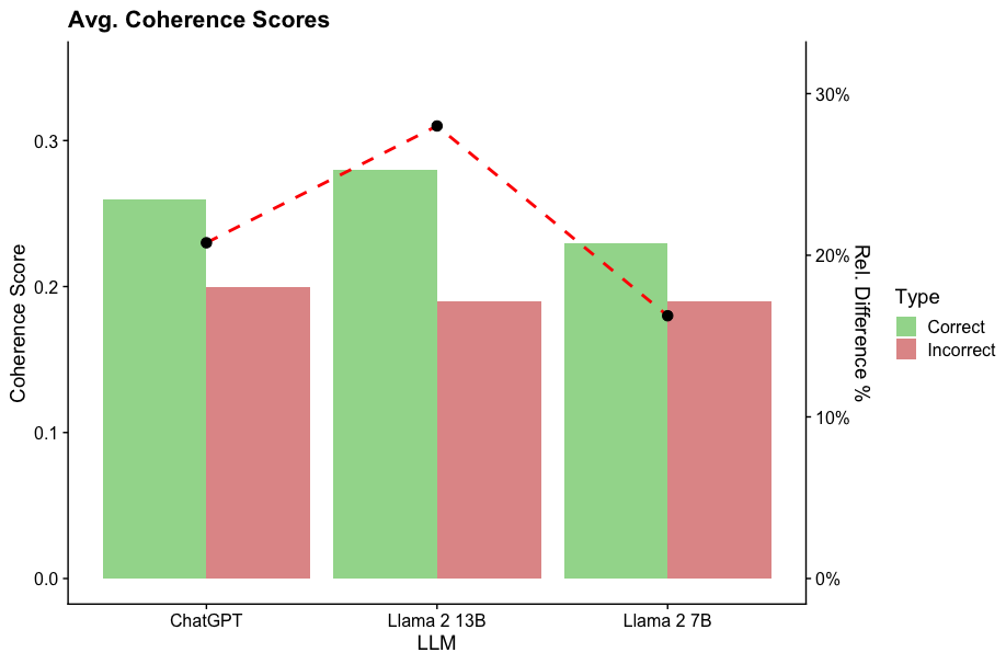Coherence. <details> <summary>extracted/6246183/coherence.png Details</summary>  ### Visual Description \n ## Bar Chart with Line Overlay: Average Coherence Scores by LLM and Response Type ### Overview The image is a dual-axis chart comparing the average coherence scores of three Large Language Models (LLMs) for "Correct" versus "Incorrect" responses. It also plots the relative percentage difference between these two scores for each model. The chart uses grouped bars for the scores and a dashed line for the percentage difference. ### Components/Axes * **Title:** "Avg. Coherence Scores" (top-left). * **Primary Y-Axis (Left):** Labeled "Coherence Score". Scale ranges from 0.0 to approximately 0.35, with major ticks at 0.0, 0.1, 0.2, and 0.3. * **Secondary Y-Axis (Right):** Labeled "Rel. Difference %". Scale ranges from 0% to approximately 35%, with major ticks at 0%, 10%, 20%, and 30%. * **X-Axis:** Labeled "LLM". Three categories are listed: "ChatGPT", "Llama 2 13B", and "Llama 2 7B". * **Legend:** Positioned on the right side of the chart, titled "Type". It defines two categories: * **Correct:** Represented by a light green color. * **Incorrect:** Represented by a light red/salmon color. * **Data Series:** 1. **Grouped Bars:** For each LLM, two bars are shown side-by-side. The left (green) bar represents the average coherence score for "Correct" responses. The right (red) bar represents the average coherence score for "Incorrect" responses. 2. **Line Overlay:** A dashed red line with black circular markers connects data points representing the "Rel. Difference %" for each LLM. This line is plotted against the right-hand Y-axis. ### Detailed Analysis **1. ChatGPT:** * **Correct (Green Bar):** Coherence Score ≈ 0.26. * **Incorrect (Red Bar):** Coherence Score ≈ 0.20. * **Rel. Difference % (Line Marker):** ≈ 20%. The black dot is positioned at the 20% tick on the right axis. **2. Llama 2 13B:** * **Correct (Green Bar):** Coherence Score ≈ 0.28 (the highest "Correct" score on the chart). * **Incorrect (Red Bar):** Coherence Score ≈ 0.19. * **Rel. Difference % (Line Marker):** ≈ 30%. The black dot is positioned at the 30% tick on the right axis, representing the peak of the dashed line. **3. Llama 2 7B:** * **Correct (Green Bar):** Coherence Score ≈ 0.23. * **Incorrect (Red Bar):** Coherence Score ≈ 0.19. * **Rel. Difference % (Line Marker):** ≈ 18%. The black dot is positioned slightly below the 20% tick on the right axis. **Trend Verification:** * For all three LLMs, the "Correct" (green) bar is taller than the "Incorrect" (red) bar, indicating a consistent trend of higher coherence scores for correct responses. * The dashed red line (Rel. Difference %) slopes upward from ChatGPT to Llama 2 13B, then slopes downward to Llama 2 7B, forming a peak at the 13B model. ### Key Observations 1. **Consistent Performance Gap:** Every model shows a higher average coherence score for correct responses compared to incorrect ones. 2. **Peak Difference at Llama 2 13B:** The relative difference between correct and incorrect coherence scores is largest for Llama 2 13B (~30%), significantly higher than for ChatGPT (~20%) or Llama 2 7B (~18%). 3. **Highest Absolute Score:** Llama 2 13B also achieves the highest absolute coherence score for correct responses (~0.28). 4. **Similar "Incorrect" Scores:** The coherence scores for incorrect responses are relatively similar across all three models, clustering around 0.19-0.20. ### Interpretation This chart suggests that while all evaluated LLMs produce more coherent text when their responses are correct, the magnitude of this coherence gap varies by model. The data indicates that **Llama 2 13B exhibits the most pronounced distinction in text quality between its correct and incorrect outputs.** This could imply that this model's architecture or training leads to a sharper degradation in linguistic coherence when it fails, compared to ChatGPT or the smaller Llama 2 7B model. The fact that the "Incorrect" coherence scores are similar across models, while the "Correct" scores vary more, suggests that the models' baseline ability to generate fluent but wrong text is comparable, but their peak performance on correct answers differs. The Llama 2 13B model appears to have a higher ceiling for coherence when it is accurate. This information is valuable for understanding model behavior beyond simple accuracy metrics, highlighting how reliability and output quality are intertwined. </details> Figure 5: An evaluation of the explanation coherence and question accuracy.The average coherence score is consistently higher for explanations corresponding to the correct hypotheses across the LLMs. Similarly to parsimony, we found coherence to be a better indicator of explanation quality being statistically significant for both GPT 3.5 and Llama 2 13B on COPA and both Llama 2 models on E-Care. We found that the average coherence score is consistently greater for the stronger hypothesis across all LLMs and datasets (see Figure 5). Both GPT and Llama 2 13B exhibit a higher relative difference between the correct and incorrect hypotheses in contrast to Llama 2 7B. 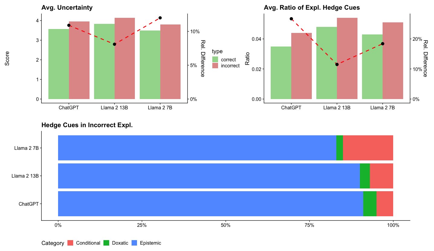Uncertainty. <details> <summary>extracted/6246183/uncertainty.png Details</summary>  ### Visual Description ## [Chart Set]: Analysis of Uncertainty and Hedge Cues in Language Model Explanations ### Overview The image contains three distinct charts analyzing the behavior of three language models (ChatGPT, Llama 2 13B, Llama 2 7B) regarding uncertainty and the use of "hedge cues" in their explanations. The top section contains two dual-axis bar charts comparing "correct" vs. "incorrect" explanations. The bottom section contains a horizontal stacked bar chart detailing the types of hedge cues found specifically in incorrect explanations. ### Components/Axes **Top-Left Chart: "Avg. Uncertainty"** * **Primary Y-Axis (Left):** Label: "Score". Scale: 0 to 4, with increments of 1. * **Secondary Y-Axis (Right):** Label: "Rel. Difference". Scale: 0% to 10%, with increments of 5%. * **X-Axis:** Categories: "ChatGPT", "Llama 2 13B", "Llama 2 7B". * **Legend:** Located between the two top charts. Title: "type". Categories: "correct" (green bar), "incorrect" (red bar). * **Data Series:** 1. **Bar Series:** Paired green ("correct") and red ("incorrect") bars for each model. 2. **Line Series:** A red dashed line with black circular markers, plotted against the right "Rel. Difference" axis. **Top-Right Chart: "Avg. Ratio of Expl. Hedge Cues"** * **Primary Y-Axis (Left):** Label: "Ratio". Scale: 0.00 to 0.04, with increments of 0.02. * **Secondary Y-Axis (Right):** Label: "Rel. Difference". Scale: 0% to 20%, with increments of 10%. * **X-Axis:** Categories: "ChatGPT", "Llama 2 13B", "Llama 2 7B". * **Legend:** Shared with the top-left chart (green="correct", red="incorrect"). * **Data Series:** 1. **Bar Series:** Paired green ("correct") and red ("incorrect") bars for each model. 2. **Line Series:** A red dashed line with black circular markers, plotted against the right "Rel. Difference" axis. **Bottom Chart: "Hedge Cues in Incorrect Expl."** * **Y-Axis:** Categories: "Llama 2 7B", "Llama 2 13B", "ChatGPT" (listed from top to bottom). * **X-Axis:** Label: Percentage scale from 0% to 100%, with markers at 0%, 25%, 50%, 75%, 100%. * **Legend:** Located at the bottom. Title: "Category". Categories: "Conditional" (red), "Doxastic" (green), "Epistemic" (blue). * **Data Series:** A single horizontal stacked bar for each model, segmented by color according to the legend. ### Detailed Analysis **1. Avg. Uncertainty Chart (Top-Left)** * **Trend Verification:** For all three models, the red "incorrect" bar is taller than the green "correct" bar, indicating higher average uncertainty scores for incorrect explanations. The red dashed line (Rel. Difference) shows a "V" shape, dipping at Llama 2 13B. * **Data Points (Approximate):** * **ChatGPT:** Correct Score ≈ 3.6, Incorrect Score ≈ 3.9. Rel. Difference ≈ 8%. * **Llama 2 13B:** Correct Score ≈ 3.8, Incorrect Score ≈ 4.1. Rel. Difference ≈ 7%. * **Llama 2 7B:** Correct Score ≈ 3.5, Incorrect Score ≈ 3.8. Rel. Difference ≈ 11% (highest relative difference). **2. Avg. Ratio of Expl. Hedge Cues Chart (Top-Right)** * **Trend Verification:** For all three models, the red "incorrect" bar is taller than the green "correct" bar, indicating a higher ratio of hedge cues in incorrect explanations. The red dashed line (Rel. Difference) shows a "check mark" shape, dipping at Llama 2 13B. * **Data Points (Approximate):** * **ChatGPT:** Correct Ratio ≈ 0.035, Incorrect Ratio ≈ 0.043. Rel. Difference ≈ 23% (highest relative difference). * **Llama 2 13B:** Correct Ratio ≈ 0.048, Incorrect Ratio ≈ 0.055. Rel. Difference ≈ 11%. * **Llama 2 7B:** Correct Ratio ≈ 0.043, Incorrect Ratio ≈ 0.051. Rel. Difference ≈ 19%. **3. Hedge Cues in Incorrect Expl. Chart (Bottom)** * **Component Isolation:** Each horizontal bar represents 100% of the hedge cues used in that model's incorrect explanations. * **Data Distribution (Approximate percentages):** * **Llama 2 7B:** Epistemic (Blue) ≈ 82%, Doxastic (Green) ≈ 3%, Conditional (Red) ≈ 15%. * **Llama 2 13B:** Epistemic (Blue) ≈ 88%, Doxastic (Green) ≈ 4%, Conditional (Red) ≈ 8%. * **ChatGPT:** Epistemic (Blue) ≈ 90%, Doxastic (Green) ≈ 5%, Conditional (Red) ≈ 5%. ### Key Observations 1. **Consistent Pattern:** Across all models, incorrect explanations are associated with both higher average uncertainty scores and a higher ratio of hedge cues compared to correct explanations. 2. **Model Comparison:** Llama 2 13B shows the highest absolute scores and ratios for both correct and incorrect explanations. However, ChatGPT and Llama 2 7B often show a larger *relative* increase (Rel. Difference) in these metrics when moving from correct to incorrect explanations. 3. **Hedge Cue Composition:** In incorrect explanations, the vast majority of hedge cues are "Epistemic" (related to knowledge or belief) across all models. "Conditional" cues are the second most common, while "Doxastic" cues (related to opinion) are rare. 4. **Inverse Relationship in Hedge Cue Ratio:** While Llama 2 13B has the highest absolute ratio of hedge cues, it has the smallest relative difference between correct and incorrect explanations. ChatGPT has the largest relative difference. ### Interpretation The data suggests a strong correlation between a language model's expression of uncertainty (both in self-reported scores and in linguistic hedging) and the factual correctness of its explanations. Incorrect answers are not just wrong; they are delivered with measurably more cautious, qualified, or uncertain language. The dominance of "Epistemic" hedge cues (e.g., "I think," "It might be") in incorrect explanations indicates that models may be using language that frames knowledge as tentative or belief-based when they are less confident or incorrect. The lower use of "Doxastic" cues suggests models rarely frame incorrect answers as mere opinion. The variation between models is notable. Llama 2 13B appears to use more hedging language overall, but the *change* in its behavior between correct and incorrect states is less pronounced than for ChatGPT or Llama 2 7B. This could imply different internal confidence calibration or different linguistic strategies for expressing uncertainty. The charts collectively provide a multi-faceted view of how model "uncertainty" manifests both as an internal score and as a communicative style, linking it directly to output quality. </details> Figure 6: Evaluation of linguistic uncertainty in LLM-generated explanations. LLMs tend to use more hedging language in explanations supporting less plausible hypotheses. Across the LLMs, the hedging language is found to be predominantly epistemic A.8. The results reveal that linguistic uncertainty is the strongest predictor of explanation quality and is a statistically significant feature for all LLMs. This suggests that LLMs use more qualifying language when explaining weaker hypotheses (see Figure 6). We found that uncertainty can improve accuracy by 13pp on COPA and 4pp on E-CARE. We also examine the uncertainty cues expressed by LLMs by analyzing both the frequency of hedge words and the types of hedge cues employed in incorrect explanations. We find the distribution of hedge cues across LLMs tends to be similar, with only minor differences between LLMs (Figure 6). Epistemic cues were most frequently used by all three models, with LLaMA 2 7B being more likely to use conditional cues. See Appendix A.8 for further details.. ### 7.1 Correlation with Human Judgement. We first sample 100 generated explanation pairs across both the COPA and E-CARE tasks and evaluated LLMs. Two human evaluators are instructed to evaluate the pair of explanations and to select which explanation is most plausible. No additional information about the original question nor the correct answer is provided to prevent biasing the judge. The human evaluators on average were able to identify the explanation associated with the correct answer 96% (COPA) and 91% (E-Care) of time. We compute the inter-evaluator agreement score between two human evaluators and find that there is Cohen’s Kappa score of .68 suggesting there is a strong agreement between the two evaluators. To evaluate if IBE-Eval is correlated with human judgment, we compute the Spearman’s rank correlation between GPT-3.5-as-a-judge, IBE-Eval and human judgment. We find that GPT-3.5-as-a-judge exhibits a weak and statistically insignificant correlation with human judgment (0.31). In contrast, we find that the IBE-Eval is significantly aligned with human preferences (with a Spearman’s correlation of 0.64 and p < 0.01) further suggesting the IBE’s potential for automatic explanation evaluation. ## 8 Related Work Explorations of LLM reasoning capabilities across various domains (e.g. arithmetic, commonsense, planning, symbolic, etc) are an emerging area of interest Xu et al. (2023); Huang and Chang (2023). Prompt-based methods Wei et al. (2022b); Zhou et al. (2023); Wang et al. (2023), such as CoT, investigate strategies to elicit specific types of reasoning behavior through direct LLM interaction. Olausson et al. (2023) investigate automatic proof generation and propose a neurosymbolic framework with an LLM semantic parser and external solver. Creswell et al. (2022) propose an inference framework where the LLM acts as both a selection and inference module to produce explanations consisting of causal reasoning steps in entailment tasks. Research on LLM faithfulness Atanasova et al. (2023) investigates if LLM explanations are robust to spurious input alterations. Parcalabescu and Frank (2024) propose a self-consistency measure CC-SHAP which measures how specific alterations to a model’s input contribute to the generated explanation. This paper primarily draws inspiration from recent work on the evaluation of natural language explanations Quan et al. (2024); Valentino et al. (2021); Wiegreffe and Marasovic (2021); Thayaparan et al. (2020); Dalvi et al. (2021); Camburu et al. (2018). However, differently from previous methods that require extensive human annotations or specific domain knowledge, we are the first to propose a set of criteria that can be automatically computed on explicit linguistic and logical features. ## 9 Conclusion This paper proposed IBE-Eval, an interpretable framework for LLM explanation evaluation inspired by philosophical accounts of Inference to the Best Explanation (IBE). IBE-Eval can identify the best explanation supporting the correct answer with up to 77% accuracy in CQA scenarios, improving upon a GPT 3.5 Judge baselines by +17%. Our regression study suggests that LLM explanations tend to conform to IBE expectations and that IBE-Eval is strongly correlated with human judgment. Linguistic uncertainty is the stronger IBE predictor for explanation quality closely followed by parsimony and coherence. However, we also found that LLMs tend to be strong conjecture models able to generate logically consistent explanations for less plausible hypotheses, suggesting limited applicability for the logical consistency criterion in isolation. We believe our findings can open new lines of research on external evaluation methods for LLMs as well as interpretability tools for understanding the LLM’s underlying explanatory process. ## 10 Limitations IBE-Eval offers an interpretable explanation evaluation framework utilizing logical and linguistic features. Our current instantiation of the framework is primarily limited in that it does not consider grounded knowledge for factuality. We observe that LLMs can generate factually incorrect but logically consistent explanations. In some cases, the coherence metric can identify those factual errors when the step-wise entailment score is comparatively lower. However, our reliance on aggregated metrics can hide weaker internal entailment especially when the explanation is longer or the entailment strength of the surrounding explanation steps is stronger. Future work can introduce metrics to evaluate grounded knowledge or perform more granular evaluations of explanations to better weight factual inaccuracies. Additionally, IBE-Eval currently does not support single natural language explanations and was evaluated in the limited domain of causal commonsense reasoning. Future work will explore globally calibrating IBE-Eval plausibility scores to extend evaluation to more diverse explanation generation and QA settings. Calibration efforts would allow for IBE-Eval to generate comparable scores across unrelated explanations and could be used to produce global thresholds explanation classification. Finally, the list of criteria considered in this work is not exhaustive and can be extended in future work. However, additional criteria for IBE might not be straightforward to implement (e.g., unification power, hardness to variation) and would probably require further progress in both epistemological accounts and existing NLP technology. ## 11 Ethics Statement The human annotators for computing the human judgment baseline are all authors of the papers and as such were not further compensated for the annotation task. ## Acknowledgements This work was partially funded by the Swiss National Science Foundation (SNSF) project NeuMath (200021_204617), by the EPSRC grant EP/T026995/1 entitled “EnnCore: End-to-End Conceptual Guarding of Neural Architectures” under Security for all in an AI-enabled society, by the CRUK National Biomarker Centre, and supported by the Manchester Experimental Cancer Medicine Centre, the Science Foundation Ireland under grants SFI/18/CRT/6223 (Centre for Research Training in Artificial Intelligence), SFI/12/RC/2289_P2 (Insight), co-funded by the European Regional Development Fund, and the NIHR Manchester Biomedical Research Centre. ## References - Atanasova et al. (2023) Pepa Atanasova, Oana-Maria Camburu, Christina Lioma, Thomas Lukasiewicz, Jakob Grue Simonsen, and Isabelle Augenstein. 2023. Faithfulness tests for natural language explanations. In Proceedings of the 61st Annual Meeting of the Association for Computational Linguistics (Volume 2: Short Papers), pages 283–294, Toronto, Canada. Association for Computational Linguistics. - Baumgartner (2015) Michael Baumgartner. 2015. Parsimony and causality. Quality & Quantity, 49:839–856. - Bowman et al. (2015) Samuel R. Bowman, Gabor Angeli, Christopher Potts, and Christopher D. Manning. 2015. A large annotated corpus for learning natural language inference. In Proceedings of the 2015 Conference on Empirical Methods in Natural Language Processing, pages 632–642, Lisbon, Portugal. Association for Computational Linguistics. - Brown et al. (2020) Tom Brown, Benjamin Mann, Nick Ryder, Melanie Subbiah, Jared D Kaplan, Prafulla Dhariwal, Arvind Neelakantan, Pranav Shyam, Girish Sastry, Amanda Askell, et al. 2020. Language models are few-shot learners. Advances in neural information processing systems, 33:1877–1901. - Buitinck et al. (2013) Lars Buitinck, Gilles Louppe, Mathieu Blondel, Fabian Pedregosa, Andreas Mueller, Olivier Grisel, Vlad Niculae, Peter Prettenhofer, Alexandre Gramfort, Jaques Grobler, Robert Layton, Jake VanderPlas, Arnaud Joly, Brian Holt, and Gaël Varoquaux. 2013. API design for machine learning software: experiences from the scikit-learn project. In ECML PKDD Workshop: Languages for Data Mining and Machine Learning, pages 108–122. - Camburu et al. (2018) Oana-Maria Camburu, Tim Rocktäschel, Thomas Lukasiewicz, and Phil Blunsom. 2018. e-snli: Natural language inference with natural language explanations. Advances in Neural Information Processing Systems, 31. - Camburu et al. (2020) OM Camburu, B Shillingford, P Minervini, T Lukasiewicz, and P Blunsom. 2020. Make up your mind! adversarial generation of inconsistent natural language explanations. In Proceedings of the 58th Annual Meeting of the Association for Computational Linguistics, 2020. ACL Anthology. - Chakraborty et al. (2017) Supriyo Chakraborty, Richard Tomsett, Ramya Raghavendra, Daniel Harborne, Moustafa Alzantot, Federico Cerutti, Mani Srivastava, Alun Preece, Simon Julier, Raghuveer M. Rao, Troy D. Kelley, Dave Braines, Murat Sensoy, Christopher J. Willis, and Prudhvi Gurram. 2017. Interpretability of deep learning models: A survey of results. In 2017 IEEE SmartWorld, Ubiquitous Intelligence & Computing, Advanced & Trusted Computed, Scalable Computing & Communications, Cloud & Big Data Computing, Internet of People and Smart City Innovation (SmartWorld/SCALCOM/UIC/ATC/CBDCom/IOP/SCI), pages 1–6. - Creswell et al. (2022) Antonia Creswell, Murray Shanahan, and Irina Higgins. 2022. Selection-inference: Exploiting large language models for interpretable logical reasoning. - Dalal et al. (2023) Dhairya Dalal, Paul Buitelaar, and Mihael Arcan. 2023. CALM-bench: A multi-task benchmark for evaluating causality-aware language models. In Findings of the Association for Computational Linguistics: EACL 2023, pages 296–311, Dubrovnik, Croatia. Association for Computational Linguistics. - Dalvi et al. (2021) Bhavana Dalvi, Peter Jansen, Oyvind Tafjord, Zhengnan Xie, Hannah Smith, Leighanna Pipatanangkura, and Peter Clark. 2021. Explaining answers with entailment trees. In Proceedings of the 2021 Conference on Empirical Methods in Natural Language Processing, pages 7358–7370. - Danilevsky et al. (2020) Marina Danilevsky, Kun Qian, Ranit Aharonov, Yannis Katsis, Ban Kawas, and Prithviraj Sen. 2020. A survey of the state of explainable AI for natural language processing. In Proceedings of the 1st Conference of the Asia-Pacific Chapter of the Association for Computational Linguistics and the 10th International Joint Conference on Natural Language Processing, pages 447–459, Suzhou, China. Association for Computational Linguistics. - Deutsch (2011) David Deutsch. 2011. The beginning of infinity: Explanations that transform the world. penguin uK. - Du et al. (2022) Li Du, Xiao Ding, Kai Xiong, Ting Liu, and Bing Qin. 2022. e-CARE: a new dataset for exploring explainable causal reasoning. In Proceedings of the 60th Annual Meeting of the Association for Computational Linguistics (Volume 1: Long Papers), pages 432–446, Dublin, Ireland. Association for Computational Linguistics. - Farkas et al. (2010) Richárd Farkas, Veronika Vincze, György Móra, János Csirik, and György Szarvas. 2010. The CoNLL-2010 shared task: Learning to detect hedges and their scope in natural language text. In Proceedings of the Fourteenth Conference on Computational Natural Language Learning – Shared Task, pages 1–12, Uppsala, Sweden. Association for Computational Linguistics. - Gao et al. (2023) Leo Gao, Jonathan Tow, Baber Abbasi, Stella Biderman, Sid Black, Anthony DiPofi, Charles Foster, Laurence Golding, Jeffrey Hsu, Alain Le Noac’h, Haonan Li, Kyle McDonell, Niklas Muennighoff, Chris Ociepa, Jason Phang, Laria Reynolds, Hailey Schoelkopf, Aviya Skowron, Lintang Sutawika, Eric Tang, Anish Thite, Ben Wang, Kevin Wang, and Andy Zou. 2023. A framework for few-shot language model evaluation. - Geirhos et al. (2020) Robert Geirhos, Jörn-Henrik Jacobsen, Claudio Michaelis, Richard Zemel, Wieland Brendel, Matthias Bethge, and Felix A Wichmann. 2020. Shortcut learning in deep neural networks. Nature Machine Intelligence, 2(11):665–673. - Gordon et al. (2012) Andrew Gordon, Zornitsa Kozareva, and Melissa Roemmele. 2012. SemEval-2012 task 7: Choice of plausible alternatives: An evaluation of commonsense causal reasoning. In *SEM 2012: The First Joint Conference on Lexical and Computational Semantics – Volume 1: Proceedings of the main conference and the shared task, and Volume 2: Proceedings of the Sixth International Workshop on Semantic Evaluation (SemEval 2012), pages 394–398, Montréal, Canada. Association for Computational Linguistics. - Harman (1965) Gilbert H Harman. 1965. The inference to the best explanation. The philosophical review, 74(1):88–95. - Honnibal and Montani (2017) Matthew Honnibal and Ines Montani. 2017. spaCy 2: Natural language understanding with Bloom embeddings, convolutional neural networks and incremental parsing. To appear. - Huang and Chang (2022) Jie Huang and Kevin Chen-Chuan Chang. 2022. Towards reasoning in large language models: A survey. arXiv preprint arXiv:2212.10403. - Huang and Chang (2023) Jie Huang and Kevin Chen-Chuan Chang. 2023. Towards reasoning in large language models: A survey. - Huang et al. (2023) Lei Huang, Weijiang Yu, Weitao Ma, Weihong Zhong, Zhangyin Feng, Haotian Wang, Qianglong Chen, Weihua Peng, Xiaocheng Feng, Bing Qin, and Ting Liu. 2023. A survey on hallucination in large language models: Principles, taxonomy, challenges, and open questions. - Ji et al. (2023) Ziwei Ji, Nayeon Lee, Rita Frieske, Tiezheng Yu, Dan Su, Yan Xu, Etsuko Ishii, Ye Jin Bang, Andrea Madotto, and Pascale Fung. 2023. Survey of hallucination in natural language generation. ACM Comput. Surv., 55(12). - Kitcher (1989) Philip Kitcher. 1989. Explanatory unification and the causal structure of the world. - Knight (2023) Will Knight. 2023. Ai is becoming more powerful-but also more secretive. - Lampinen et al. (2022) Andrew Lampinen, Ishita Dasgupta, Stephanie Chan, Kory Mathewson, Mh Tessler, Antonia Creswell, James McClelland, Jane Wang, and Felix Hill. 2022. Can language models learn from explanations in context? In Findings of the Association for Computational Linguistics: EMNLP 2022, pages 537–563. - Laskar et al. (2023) Md Tahmid Rahman Laskar, M Saiful Bari, Mizanur Rahman, Md Amran Hossen Bhuiyan, Shafiq Joty, and Jimmy Xiangji Huang. 2023. A systematic study and comprehensive evaluation of chatgpt on benchmark datasets. - Liang et al. (2023) Percy Liang, Rishi Bommasani, Tony Lee, Dimitris Tsipras, Dilara Soylu, Michihiro Yasunaga, Yian Zhang, Deepak Narayanan, Yuhuai Wu, Ananya Kumar, Benjamin Newman, Binhang Yuan, Bobby Yan, Ce Zhang, Christian Cosgrove, Christopher D. Manning, Christopher Ré, Diana Acosta-Navas, Drew A. Hudson, Eric Zelikman, Esin Durmus, Faisal Ladhak, Frieda Rong, Hongyu Ren, Huaxiu Yao, Jue Wang, Keshav Santhanam, Laurel Orr, Lucia Zheng, Mert Yuksekgonul, Mirac Suzgun, Nathan Kim, Neel Guha, Niladri Chatterji, Omar Khattab, Peter Henderson, Qian Huang, Ryan Chi, Sang Michael Xie, Shibani Santurkar, Surya Ganguli, Tatsunori Hashimoto, Thomas Icard, Tianyi Zhang, Vishrav Chaudhary, William Wang, Xuechen Li, Yifan Mai, Yuhui Zhang, and Yuta Koreeda. 2023. Holistic evaluation of language models. - Lipton (2017) Peter Lipton. 2017. Inference to the best explanation. A Companion to the Philosophy of Science, pages 184–193. - Lombrozo (2012) Tania Lombrozo. 2012. Explanation and abductive inference. Oxford handbook of thinking and reasoning, pages 260–276. - Mackonis (2013) Adolfas Mackonis. 2013. Inference to the best explanation, coherence and other explanatory virtues. Synthese, 190(6):975–995. - Nie et al. (2019) Yixin Nie, Haonan Chen, and Mohit Bansal. 2019. Combining fact extraction and verification with neural semantic matching networks. In Association for the Advancement of Artificial Intelligence (AAAI). - Nie et al. (2020) Yixin Nie, Adina Williams, Emily Dinan, Mohit Bansal, Jason Weston, and Douwe Kiela. 2020. Adversarial NLI: A new benchmark for natural language understanding. In Proceedings of the 58th Annual Meeting of the Association for Computational Linguistics. Association for Computational Linguistics. - Olausson et al. (2023) Theo X. Olausson, Alex Gu, Benjamin Lipkin, Cedegao E. Zhang, Armando Solar-Lezama, Joshua B. Tenenbaum, and Roger Levy. 2023. Linc: A neurosymbolic approach for logical reasoning by combining language models with first-order logic provers. - Parcalabescu and Frank (2024) Letitia Parcalabescu and Anette Frank. 2024. On measuring faithfulness or self-consistency of natural language explanations. - Pei and Jurgens (2021) Jiaxin Pei and David Jurgens. 2021. Measuring sentence-level and aspect-level (un)certainty in science communications. In Proceedings of the 2021 Conference on Empirical Methods in Natural Language Processing, pages 9959–10011, Online and Punta Cana, Dominican Republic. Association for Computational Linguistics. - Popper (2014) Karl Popper. 2014. Conjectures and refutations: The growth of scientific knowledge. routledge. - Quan et al. (2024) Xin Quan, Marco Valentino, Louise A Dennis, and André Freitas. 2024. Enhancing ethical explanations of large language models through iterative symbolic refinement. arXiv preprint arXiv:2402.00745. - R Core Team (2013) R Core Team. 2013. R: A Language and Environment for Statistical Computing. R Foundation for Statistical Computing, Vienna, Austria. ISBN 3-900051-07-0. - Sober (1981) Elliott Sober. 1981. The principle of parsimony. The British Journal for the Philosophy of Science, 32(2):145–156. - Srivastava et al. (2023) Aarohi Srivastava, Abhinav Rastogi, Abhishek Rao, Abu Awal Md Shoeb, Abubakar Abid, Adam Fisch, Adam R. Brown, Adam Santoro, Aditya Gupta, Adrià Garriga-Alonso, Agnieszka Kluska, Aitor Lewkowycz, Akshat Agarwal, Alethea Power, Alex Ray, Alex Warstadt, Alexander W. Kocurek, Ali Safaya, Ali Tazarv, Alice Xiang, Alicia Parrish, Allen Nie, Aman Hussain, Amanda Askell, Amanda Dsouza, Ambrose Slone, Ameet Rahane, Anantharaman S. Iyer, Anders Andreassen, Andrea Madotto, Andrea Santilli, Andreas Stuhlmüller, Andrew Dai, Andrew La, Andrew Lampinen, Andy Zou, Angela Jiang, Angelica Chen, Anh Vuong, Animesh Gupta, Anna Gottardi, Antonio Norelli, Anu Venkatesh, Arash Gholamidavoodi, Arfa Tabassum, Arul Menezes, Arun Kirubarajan, Asher Mullokandov, Ashish Sabharwal, Austin Herrick, Avia Efrat, Aykut Erdem, Ayla Karakaş, B. Ryan Roberts, Bao Sheng Loe, Barret Zoph, Bartłomiej Bojanowski, Batuhan Özyurt, Behnam Hedayatnia, Behnam Neyshabur, Benjamin Inden, Benno Stein, Berk Ekmekci, Bill Yuchen Lin, Blake Howald, Bryan Orinion, Cameron Diao, Cameron Dour, Catherine Stinson, Cedrick Argueta, César Ferri Ramírez, Chandan Singh, Charles Rathkopf, Chenlin Meng, Chitta Baral, Chiyu Wu, Chris Callison-Burch, Chris Waites, Christian Voigt, Christopher D. Manning, Christopher Potts, Cindy Ramirez, Clara E. Rivera, Clemencia Siro, Colin Raffel, Courtney Ashcraft, Cristina Garbacea, Damien Sileo, Dan Garrette, Dan Hendrycks, Dan Kilman, Dan Roth, Daniel Freeman, Daniel Khashabi, Daniel Levy, Daniel Moseguí González, Danielle Perszyk, Danny Hernandez, Danqi Chen, Daphne Ippolito, Dar Gilboa, David Dohan, David Drakard, David Jurgens, Debajyoti Datta, Deep Ganguli, Denis Emelin, Denis Kleyko, Deniz Yuret, Derek Chen, Derek Tam, Dieuwke Hupkes, Diganta Misra, Dilyar Buzan, Dimitri Coelho Mollo, Diyi Yang, Dong-Ho Lee, Dylan Schrader, Ekaterina Shutova, Ekin Dogus Cubuk, Elad Segal, Eleanor Hagerman, Elizabeth Barnes, Elizabeth Donoway, Ellie Pavlick, Emanuele Rodola, Emma Lam, Eric Chu, Eric Tang, Erkut Erdem, Ernie Chang, Ethan A. Chi, Ethan Dyer, Ethan Jerzak, Ethan Kim, Eunice Engefu Manyasi, Evgenii Zheltonozhskii, Fanyue Xia, Fatemeh Siar, Fernando Martínez-Plumed, Francesca Happé, Francois Chollet, Frieda Rong, Gaurav Mishra, Genta Indra Winata, Gerard de Melo, Germán Kruszewski, Giambattista Parascandolo, Giorgio Mariani, Gloria Wang, Gonzalo Jaimovitch-López, Gregor Betz, Guy Gur-Ari, Hana Galijasevic, Hannah Kim, Hannah Rashkin, Hannaneh Hajishirzi, Harsh Mehta, Hayden Bogar, Henry Shevlin, Hinrich Schütze, Hiromu Yakura, Hongming Zhang, Hugh Mee Wong, Ian Ng, Isaac Noble, Jaap Jumelet, Jack Geissinger, Jackson Kernion, Jacob Hilton, Jaehoon Lee, Jaime Fernández Fisac, James B. Simon, James Koppel, James Zheng, James Zou, Jan Kocoń, Jana Thompson, Janelle Wingfield, Jared Kaplan, Jarema Radom, Jascha Sohl-Dickstein, Jason Phang, Jason Wei, Jason Yosinski, Jekaterina Novikova, Jelle Bosscher, Jennifer Marsh, Jeremy Kim, Jeroen Taal, Jesse Engel, Jesujoba Alabi, Jiacheng Xu, Jiaming Song, Jillian Tang, Joan Waweru, John Burden, John Miller, John U. Balis, Jonathan Batchelder, Jonathan Berant, Jörg Frohberg, Jos Rozen, Jose Hernandez-Orallo, Joseph Boudeman, Joseph Guerr, Joseph Jones, Joshua B. Tenenbaum, Joshua S. Rule, Joyce Chua, Kamil Kanclerz, Karen Livescu, Karl Krauth, Karthik Gopalakrishnan, Katerina Ignatyeva, Katja Markert, Kaustubh D. Dhole, Kevin Gimpel, Kevin Omondi, Kory Mathewson, Kristen Chiafullo, Ksenia Shkaruta, Kumar Shridhar, Kyle McDonell, Kyle Richardson, Laria Reynolds, Leo Gao, Li Zhang, Liam Dugan, Lianhui Qin, Lidia Contreras-Ochando, Louis-Philippe Morency, Luca Moschella, Lucas Lam, Lucy Noble, Ludwig Schmidt, Luheng He, Luis Oliveros Colón, Luke Metz, Lütfi Kerem Şenel, Maarten Bosma, Maarten Sap, Maartje ter Hoeve, Maheen Farooqi, Manaal Faruqui, Mantas Mazeika, Marco Baturan, Marco Marelli, Marco Maru, Maria Jose Ramírez Quintana, Marie Tolkiehn, Mario Giulianelli, Martha Lewis, Martin Potthast, Matthew L. Leavitt, Matthias Hagen, Mátyás Schubert, Medina Orduna Baitemirova, Melody Arnaud, Melvin McElrath, Michael A. Yee, Michael Cohen, Michael Gu, Michael Ivanitskiy, Michael Starritt, Michael Strube, Michał Swędrowski, Michele Bevilacqua, Michihiro Yasunaga, Mihir Kale, Mike Cain, Mimee Xu, Mirac Suzgun, Mitch Walker, Mo Tiwari, Mohit Bansal, Moin Aminnaseri, Mor Geva, Mozhdeh Gheini, Mukund Varma T, Nanyun Peng, Nathan A. Chi, Nayeon Lee, Neta Gur-Ari Krakover, Nicholas Cameron, Nicholas Roberts, Nick Doiron, Nicole Martinez, Nikita Nangia, Niklas Deckers, Niklas Muennighoff, Nitish Shirish Keskar, Niveditha S. Iyer, Noah Constant, Noah Fiedel, Nuan Wen, Oliver Zhang, Omar Agha, Omar Elbaghdadi, Omer Levy, Owain Evans, Pablo Antonio Moreno Casares, Parth Doshi, Pascale Fung, Paul Pu Liang, Paul Vicol, Pegah Alipoormolabashi, Peiyuan Liao, Percy Liang, Peter Chang, Peter Eckersley, Phu Mon Htut, Pinyu Hwang, Piotr Miłkowski, Piyush Patil, Pouya Pezeshkpour, Priti Oli, Qiaozhu Mei, Qing Lyu, Qinlang Chen, Rabin Banjade, Rachel Etta Rudolph, Raefer Gabriel, Rahel Habacker, Ramon Risco, Raphaël Millière, Rhythm Garg, Richard Barnes, Rif A. Saurous, Riku Arakawa, Robbe Raymaekers, Robert Frank, Rohan Sikand, Roman Novak, Roman Sitelew, Ronan LeBras, Rosanne Liu, Rowan Jacobs, Rui Zhang, Ruslan Salakhutdinov, Ryan Chi, Ryan Lee, Ryan Stovall, Ryan Teehan, Rylan Yang, Sahib Singh, Saif M. Mohammad, Sajant Anand, Sam Dillavou, Sam Shleifer, Sam Wiseman, Samuel Gruetter, Samuel R. Bowman, Samuel S. Schoenholz, Sanghyun Han, Sanjeev Kwatra, Sarah A. Rous, Sarik Ghazarian, Sayan Ghosh, Sean Casey, Sebastian Bischoff, Sebastian Gehrmann, Sebastian Schuster, Sepideh Sadeghi, Shadi Hamdan, Sharon Zhou, Shashank Srivastava, Sherry Shi, Shikhar Singh, Shima Asaadi, Shixiang Shane Gu, Shubh Pachchigar, Shubham Toshniwal, Shyam Upadhyay, Shyamolima, Debnath, Siamak Shakeri, Simon Thormeyer, Simone Melzi, Siva Reddy, Sneha Priscilla Makini, Soo-Hwan Lee, Spencer Torene, Sriharsha Hatwar, Stanislas Dehaene, Stefan Divic, Stefano Ermon, Stella Biderman, Stephanie Lin, Stephen Prasad, Steven T. Piantadosi, Stuart M. Shieber, Summer Misherghi, Svetlana Kiritchenko, Swaroop Mishra, Tal Linzen, Tal Schuster, Tao Li, Tao Yu, Tariq Ali, Tatsu Hashimoto, Te-Lin Wu, Théo Desbordes, Theodore Rothschild, Thomas Phan, Tianle Wang, Tiberius Nkinyili, Timo Schick, Timofei Kornev, Titus Tunduny, Tobias Gerstenberg, Trenton Chang, Trishala Neeraj, Tushar Khot, Tyler Shultz, Uri Shaham, Vedant Misra, Vera Demberg, Victoria Nyamai, Vikas Raunak, Vinay Ramasesh, Vinay Uday Prabhu, Vishakh Padmakumar, Vivek Srikumar, William Fedus, William Saunders, William Zhang, Wout Vossen, Xiang Ren, Xiaoyu Tong, Xinran Zhao, Xinyi Wu, Xudong Shen, Yadollah Yaghoobzadeh, Yair Lakretz, Yangqiu Song, Yasaman Bahri, Yejin Choi, Yichi Yang, Yiding Hao, Yifu Chen, Yonatan Belinkov, Yu Hou, Yufang Hou, Yuntao Bai, Zachary Seid, Zhuoye Zhao, Zijian Wang, Zijie J. Wang, Zirui Wang, and Ziyi Wu. 2023. Beyond the imitation game: Quantifying and extrapolating the capabilities of language models. - Thagard (1989) Paul Thagard. 1989. Explanatory coherence. Behavioral and brain sciences, 12(3):435–467. - Thagard (1978) Paul R Thagard. 1978. The best explanation: Criteria for theory choice. The journal of philosophy, 75(2):76–92. - Thayaparan et al. (2020) Mokanarangan Thayaparan, Marco Valentino, and André Freitas. 2020. A survey on explainability in machine reading comprehension. arXiv preprint arXiv:2010.00389. - Touvron et al. (2023) Hugo Touvron, Louis Martin, Kevin Stone, Peter Albert, Amjad Almahairi, Yasmine Babaei, Nikolay Bashlykov, Soumya Batra, Prajjwal Bhargava, Shruti Bhosale, Dan Bikel, Lukas Blecher, Cristian Canton Ferrer, Moya Chen, Guillem Cucurull, David Esiobu, Jude Fernandes, Jeremy Fu, Wenyin Fu, Brian Fuller, Cynthia Gao, Vedanuj Goswami, Naman Goyal, Anthony Hartshorn, Saghar Hosseini, Rui Hou, Hakan Inan, Marcin Kardas, Viktor Kerkez, Madian Khabsa, Isabel Kloumann, Artem Korenev, Punit Singh Koura, Marie-Anne Lachaux, Thibaut Lavril, Jenya Lee, Diana Liskovich, Yinghai Lu, Yuning Mao, Xavier Martinet, Todor Mihaylov, Pushkar Mishra, Igor Molybog, Yixin Nie, Andrew Poulton, Jeremy Reizenstein, Rashi Rungta, Kalyan Saladi, Alan Schelten, Ruan Silva, Eric Michael Smith, Ranjan Subramanian, Xiaoqing Ellen Tan, Binh Tang, Ross Taylor, Adina Williams, Jian Xiang Kuan, Puxin Xu, Zheng Yan, Iliyan Zarov, Yuchen Zhang, Angela Fan, Melanie Kambadur, Sharan Narang, Aurelien Rodriguez, Robert Stojnic, Sergey Edunov, and Thomas Scialom. 2023. Llama 2: Open foundation and fine-tuned chat models. - Valentino and Freitas (2022) Marco Valentino and André Freitas. 2022. Scientific explanation and natural language: A unified epistemological-linguistic perspective for explainable ai. arXiv preprint arXiv:2205.01809. - Valentino et al. (2021) Marco Valentino, Ian Pratt-Hartmann, and André Freitas. 2021. Do natural language explanations represent valid logical arguments? verifying entailment in explainable NLI gold standards. In Proceedings of the 14th International Conference on Computational Semantics (IWCS), pages 76–86, Groningen, The Netherlands (online). Association for Computational Linguistics. - Wang et al. (2019) Alex Wang, Yada Pruksachatkun, Nikita Nangia, Amanpreet Singh, Julian Michael, Felix Hill, Omer Levy, and Samuel R. Bowman. 2019. Superglue: A stickier benchmark for general-purpose language understanding systems. CoRR, abs/1905.00537. - Wang et al. (2023) Xuezhi Wang, Jason Wei, Dale Schuurmans, Quoc Le, Ed Chi, Sharan Narang, Aakanksha Chowdhery, and Denny Zhou. 2023. Self-consistency improves chain of thought reasoning in language models. - Weber et al. (2019) Leon Weber, Pasquale Minervini, Jannes Münchmeyer, Ulf Leser, and Tim Rocktäschel. 2019. Nlprolog: Reasoning with weak unification for question answering in natural language. - Wei et al. (2022a) Jason Wei, Xuezhi Wang, Dale Schuurmans, Maarten Bosma, Ed H. Chi, Quoc Le, and Denny Zhou. 2022a. Chain of thought prompting elicits reasoning in large language models. CoRR, abs/2201.11903. - Wei et al. (2022b) Jason Wei, Xuezhi Wang, Dale Schuurmans, Maarten Bosma, Fei Xia, Ed Chi, Quoc V Le, Denny Zhou, et al. 2022b. Chain-of-thought prompting elicits reasoning in large language models. Advances in Neural Information Processing Systems, 35:24824–24837. - Wiegreffe and Marasovic (2021) Sarah Wiegreffe and Ana Marasovic. 2021. Teach me to explain: A review of datasets for explainable natural language processing. In Thirty-fifth Conference on Neural Information Processing Systems Datasets and Benchmarks Track (Round 1). - Williams et al. (2018) Adina Williams, Nikita Nangia, and Samuel Bowman. 2018. A broad-coverage challenge corpus for sentence understanding through inference. In Proceedings of the 2018 Conference of the North American Chapter of the Association for Computational Linguistics: Human Language Technologies, Volume 1 (Long Papers), pages 1112–1122. Association for Computational Linguistics. - Wu et al. (2022) Yuhuai Wu, Albert Q. Jiang, Wenda Li, Markus N. Rabe, Charles Staats, Mateja Jamnik, and Christian Szegedy. 2022. Autoformalization with large language models. - Xiang (2023) Chloe Xiang. 2023. Openai’s gpt-4 is closed source and shrouded in secrecy. - Xu et al. (2023) Fangzhi Xu, Qika Lin, Jiawei Han, Tianzhe Zhao, Jun Liu, and Erik Cambria. 2023. Are large language models really good logical reasoners? a comprehensive evaluation and beyond. - Zheng et al. (2023) Lianmin Zheng, Wei-Lin Chiang, Ying Sheng, Siyuan Zhuang, Zhanghao Wu, Yonghao Zhuang, Zi Lin, Zhuohan Li, Dacheng Li, Eric P. Xing, Haotong Zhang, Joseph Gonzalez, and Ion Stoica. 2023. Judging llm-as-a-judge with mt-bench and chatbot arena. ArXiv, abs/2306.05685. - Zhou et al. (2023) Denny Zhou, Nathanael Schärli, Le Hou, Jason Wei, Nathan Scales, Xuezhi Wang, Dale Schuurmans, Claire Cui, Olivier Bousquet, Quoc Le, and Ed Chi. 2023. Least-to-most prompting enables complex reasoning in large language models. ## Appendix A Appendix ### A.1 Reproducibility All experimental code is available online https://github.com/dhairyadalal/IBE-eval to encourage future research in the field. We additionally summarize all the model implementations and technical resources used for the computation of the proposed IBE criteria below: - We adopt the Prolog solver for neuro-symbolic integration from Quan et al. (2024). - We use Spacy Honnibal and Montani (2017) to tokenize and extract part-of-speech (POS) tags. - To compute coherence, we employ the RoBERTa-based NLI model Nie et al. (2020) that has been finetuned on a range of NLI and fact verification datasets consisting of SNLI Bowman et al. (2015), aNLI Nie et al. (2020), multilingual NLI Williams et al. (2018)), and FEVER-NLI Nie et al. (2019). - To measure sentence-level uncertainty, we employ a finetuned RoBERTa model provided by Pei and Jurgens (2021). - We use a fine-tuned BERT-based token classification model to classify all the words in the generated explanation with uncertainty categories introduced in the 2010 CoNLL shared task on Hedge Detection Farkas et al. (2010). 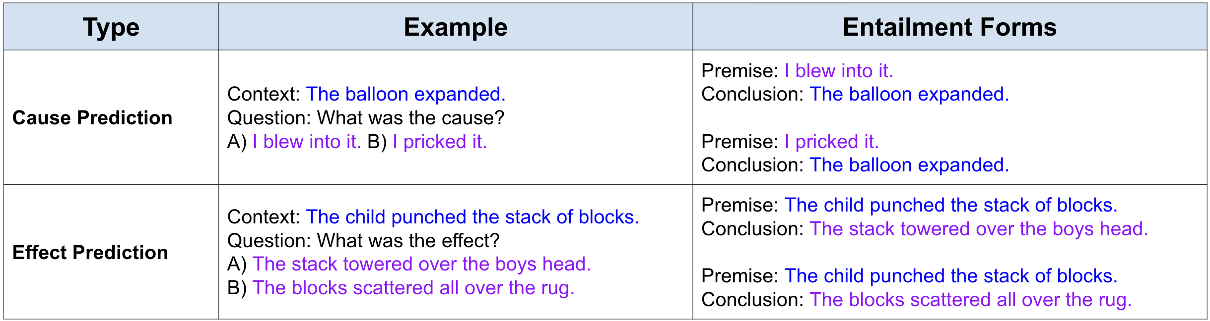### A.2 Explanation Prompting <details> <summary>extracted/6246183/eev.png Details</summary>  ### Visual Description \n ## Table: Cause and Effect Prediction with Entailment Forms ### Overview The image displays a structured table with three columns and two main data rows. It appears to be an educational or technical illustration defining two types of prediction tasks ("Cause Prediction" and "Effect Prediction") and providing examples of how these tasks can be framed as logical entailment problems. The table uses color-coding (blue and purple text) to distinguish different components of the examples. ### Components/Axes The table has the following structure: * **Column Headers (Top Row):** * **Type** (Left column) * **Example** (Center column) * **Entailment Forms** (Right column) * **Data Rows:** Two rows corresponding to the two "Type" entries. * **Color Coding:** * **Blue Text:** Used for the "Context" sentences and the "Conclusion" sentences in the Entailment Forms. * **Purple Text:** Used for the answer options (A, B) in the Example column and the "Premise" sentences in the Entailment Forms. ### Detailed Analysis The table content is presented below in a structured format: | Type | Example | Entailment Forms | |------|---------|------------------| | Cause Prediction | Context: <span style="color:blue">The balloon expanded.</span><br>Question: What was the cause?<br>A) <span style="color:purple">I blew into it.</span> B) <span style="color:purple">I pricked it.</span> | Premise: <span style="color:purple">I blew into it.</span> Conclusion: <span style="color:blue">The balloon expanded.</span><br>Premise: <span style="color:purple">I pricked it.</span> Conclusion: <span style="color:blue">The balloon expanded.</span> | | Effect Prediction | Context: <span style="color:blue">The child punched the stack of blocks.</span><br>Question: What was the effect?<br>A) <span style="color:purple">The stack towered over the boys head.</span> B) <span style="color:purple">The blocks scattered all over the rug.</span> | Premise: <span style="color:purple">The child punched the stack of blocks.</span> Conclusion: <span style="color:blue">The stack towered over the boys head.</span><br>Premise: <span style="color:purple">The child punched the stack of blocks.</span> Conclusion: <span style="color:blue">The blocks scattered all over the rug.</span> | ### Key Observations 1. **Structural Pattern:** Each "Type" is illustrated with a single context, a question, and two possible answers (A and B). These are then reformulated into two "Entailment Forms," each consisting of a premise (derived from one of the answer options) and a conclusion (the original context sentence). 2. **Logical Consistency:** The entailment forms for "Cause Prediction" present a logical issue. The premise "I pricked it" does not logically entail the conclusion "The balloon expanded" (pricking typically causes deflation). This suggests the table may be illustrating the *structure* of the task rather than asserting the logical validity of every example. 3. **Color Function:** The consistent color coding (blue for outcomes/conclusions, purple for actions/premises) helps visually map the components between the "Example" and "Entailment Forms" columns. 4. **Spatial Layout:** The "Entailment Forms" column is the widest, accommodating the paired premise-conclusion statements. The "Type" column is the narrowest. ### Interpretation This table serves as a clear, structured reference for defining and exemplifying two specific natural language processing or reasoning tasks: **Cause Prediction** and **Effect Prediction**. * **What it demonstrates:** It shows how a multiple-choice question format (Context + Question + Options) can be decomposed into a set of logical entailment pairs. This is a common technique in dataset creation for training or evaluating AI models on causal reasoning. * **Relationship between elements:** The "Example" column presents the task in a human-readable QA format. The "Entailment Forms" column translates this into a formal, machine-friendly structure where a model must judge if a premise (an action) logically leads to a conclusion (an outcome). * **Notable Anomaly:** The second "Cause Prediction" entailment ("I pricked it" → "The balloon expanded") is factually incorrect in the real world. This is likely intentional to illustrate that the *form* of the task is being presented, not necessarily a set of correct factual statements. It highlights that the task for an AI would be to distinguish between the valid and invalid entailment pairs. * **Purpose:** The table is likely from a research paper, technical report, or educational material explaining how to frame causal reasoning problems for computational models. It provides a template for converting intuitive questions into a standardized format suitable for systematic analysis or model training. </details> Figure 7: To perform IBE we convert the CQA context and answer candidates into an entailment form (i.e., EEV) Valentino et al. (2021). 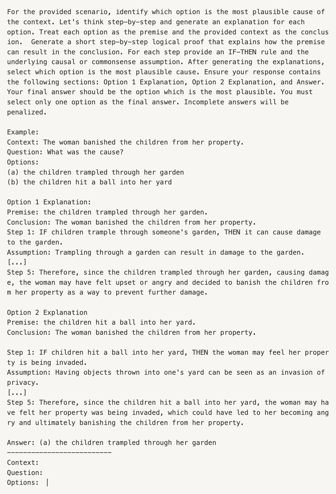<details> <summary>extracted/6246183/cot-prompt.png Details</summary>  ### Visual Description \n ## Text-Based Instructional Document: Logical Reasoning Example ### Overview The image is a screenshot or digital document containing a detailed instructional example for a causal reasoning task. It provides a structured methodology for analyzing scenarios to determine the most plausible cause of an event, using a step-by-step logical proof format. The document is entirely textual, with no charts, diagrams, or visual data elements. The language is English. ### Content Details The document is structured as follows: 1. **Initial Instructions:** A paragraph outlines the task: to identify the most plausible cause of a given context from provided options. It specifies the required methodology: * Treat each option as a premise and the context as the conclusion. * Generate a short, step-by-step logical proof for each. * For each step, provide an IF-THEN rule and the underlying causal or commonsense assumption. * Structure the final response with sections: "Option 1 Explanation," "Option 2 Explanation," and "Answer." * The final answer must select only one option. 2. **Example Section:** A complete worked example is provided. * **Context:** "The woman banished the children from her property." * **Question:** "What was the cause?" * **Options:** * (a) the children trampled through her garden * (b) the children hit a ball into her yard * **Option 1 Explanation:** * **Premise:** the children trampled through her garden. * **Conclusion:** The woman banished the children from her property. * **Step 1:** IF children trample through someone's garden, THEN it can cause damage to the garden. * **Assumption:** Trampling through a garden can result in damage to the garden. * **[...]:** Indicates omitted intermediate steps. * **Step 5:** Therefore, since the children trampled through her garden, causing damage, the woman may have felt upset or angry and decided to banish the children from her property as a way to prevent further damage. * **Option 2 Explanation:** * **Premise:** the children hit a ball into her yard. * **Conclusion:** The woman banished the children from her property. * **Step 1:** IF children hit a ball into her yard, THEN the woman may feel her property is being invaded. * **Assumption:** Having objects thrown into one's yard can be seen as an invasion of privacy. * **[...]:** Indicates omitted intermediate steps. * **Step 5:** Therefore, since the children hit a ball into her yard, the woman may have felt her property was being invaded, which could have led to her becoming angry and ultimately banishing the children from her property. * **Answer:** "(a) the children trampled through her garden" 3. **Template Footer:** The document ends with a separator line and placeholders for a new problem: * `Context:` * `Question:` * `Options: |` (The cursor `|` suggests this is an editable template). ### Key Observations * **Structured Methodology:** The document enforces a rigorous, repeatable analytical framework. It moves from a general instruction to a concrete example, demonstrating the application of the rules. * **Logical Scaffolding:** The explanations explicitly separate the logical step (IF-THEN rule) from the underlying commonsense assumption, highlighting the reasoning process. * **Implicit Bias in Example:** The chosen example and its resolution favor the option involving direct, tangible damage ("trampled through her garden") over a more minor intrusion ("hit a ball into her yard") as the more plausible cause for a severe reaction like banishment. * **Template Design:** The footer indicates this is likely a template or a prompt from an interactive system where a user would input a new context, question, and options to be analyzed using the demonstrated method. ### Interpretation This document is not a source of empirical data but a **procedural guide for logical analysis**. Its primary purpose is pedagogical or operational: to teach or enforce a specific method for causal inference. * **What it demonstrates:** It models how to deconstruct a causal claim into a chain of logical inferences supported by commonsense knowledge. The "IF-THEN" structure formalizes the reasoning, while the "Assumption" makes the underlying world knowledge explicit. * **Relationship between elements:** The instructions define the rules, the example illustrates their application, and the template invites practice. The flow is from theory to demonstration to application. * **Notable pattern:** The example's conclusion aligns with a common heuristic that more direct, harmful actions are more likely to provoke strong reactions than indirect or minor ones. This reveals an embedded commonsense bias within the logical framework itself. * **Purpose:** This format is likely used in fields like artificial intelligence (for training reasoning models), logic education, or structured decision-making processes to ensure consistent and transparent causal analysis. The image itself contains no factual data about the world; it contains data about *a method for thinking about the world*. </details> Figure 8: An example of the modified CoT prompt template for explanation generation. A modified CoT prompt is used to instruct the LLM to generate explanations. The prompt includes a set of instructions for explanation generation and an in-context example. Appended to the end of the prompt are the CQA context, causal question, and answer candidates. The LLM is instructed to first convert the options into the EEV format consisting of a premise and conclusion. The EEV format will differ depending on the directionality of the causal question (see Figure 7). Cause prediction questions will treat the answer candidate as the premise and the context as the conclusion. In contrast, effect prediction reverses the relationship treating the context as the premise and the answer options as the conclusion. After the EEV conversion, the model is instructed to generate a step-by-step explanation consisting of IF-THEN statements and the associated causal or commonsense assumptions. For ease of post-processing, the LLM is instructed to use headers and enumerate steps using the Step # format. A full example of the prompt template is exhibited in Figure 8. 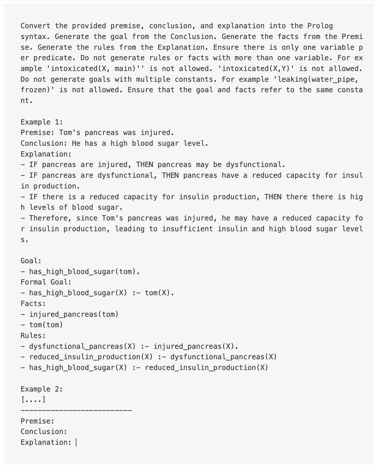<details> <summary>extracted/6246183/autoformalization.png Details</summary>  ### Visual Description ## Technical Document: Prolog Syntax Conversion Instructions ### Overview The image is a screenshot of a technical document or prompt providing instructions and an example for converting natural language logical arguments (premise, conclusion, explanation) into Prolog syntax. The document outlines specific constraints for the conversion process and provides a complete worked example. ### Document Structure The document is structured as follows: 1. **Instruction Block:** A paragraph at the top detailing the conversion task and its constraints. 2. **Example 1:** A complete, worked example showing the input (Premise, Conclusion, Explanation) and the desired output (Goal, Formal Goal, Facts, Rules). 3. **Example 2:** A placeholder for a second example, which is incomplete, showing only the input headers. ### Content Details #### 1. Instruction Block (Top of Image) The text provides the following rules for conversion: * **Task:** Convert a provided premise, conclusion, and explanation into Prolog syntax. * **Output Generation:** * Generate the **goal** from the Conclusion. * Generate the **facts** from the Premise. * Generate the **rules** from the Explanation. * **Syntactic Constraints:** * Ensure there is only **one variable per predicate**. * Do not generate rules or facts with more than one variable. Example given: `'intoxicated(X, main)'` and `'intoxicated(X,Y)'` are not allowed. * Do not generate goals with multiple constants. Example given: `'leaking(water_pipe, frozen)'` is not allowed. * Ensure that the **goal and facts refer to the same constant**. #### 2. Example 1 (Complete) **Input:** * **Premise:** `Tom's pancreas was injured.` * **Conclusion:** `He has a high blood sugar level.` * **Explanation:** * `- IF pancreas are injured, THEN pancreas may be dysfunctional.` * `- IF pancreas are dysfunctional, THEN pancreas have a reduced capacity for insulin production.` * `- IF there is a reduced capacity for insulin production, THEN there there is high levels of blood sugar.` * `- Therefore, since Tom's pancreas was injured, he may have a reduced capacity for insulin production, leading to insufficient insulin and high blood sugar levels.` **Output (Prolog Syntax):** * **Goal:** * `- has_high_blood_sugar(tom).` * **Formal Goal:** * `- has_high_blood_sugar(X) :- tom(X).` * **Facts:** * `- injured_pancreas(tom)` * `- tom(tom)` * **Rules:** * `- dysfunctional_pancreas(X) :- injured_pancreas(X).` * `- reduced_insulin_production(X) :- dysfunctional_pancreas(X)` * `- has_high_blood_sugar(X) :- reduced_insulin_production(X)` #### 3. Example 2 (Incomplete) The image shows the beginning of a second example, which is truncated. * **Header:** `Example 2:` * **Placeholder:** `[....]` * **Input Headers (Empty):** * `Premise:` * `Conclusion:` * `Explanation: |` (The cursor `|` is visible, indicating this is a template or active input field). ### Key Observations 1. **Constraint Adherence:** The Prolog code in Example 1 strictly follows the stated constraints. All predicates (`injured_pancreas`, `tom`, `dysfunctional_pancreas`, etc.) use a single variable `X`. The goal `has_high_blood_sugar(tom)` and facts use the same constant `tom`. 2. **Logical Flow:** The rules directly mirror the causal chain described in the Explanation, creating a clear deductive path from the initial fact (`injured_pancreas`) to the final conclusion (`has_high_blood_sugar`). 3. **Structural Pattern:** The output follows a consistent pattern: a simple goal, a formal goal with a variable, facts derived from the premise, and rules derived from the explanation's conditional statements. 4. **Document State:** The presence of `[....]` and the cursor in Example 2 suggests this is a template or a work-in-progress document, possibly from an interactive coding environment or a tutorial. ### Interpretation This document serves as a **specification and tutorial** for a specific formalization task. It teaches how to translate informal, natural language reasoning into a formal, logical programming language (Prolog). The core principle is **atomization**: breaking down complex statements into atomic facts and simple, single-variable rules. The example demonstrates a **reductive logical chain**. The explanation provides a multi-step causal argument, which is reduced to a series of Prolog rules where each rule's head is the consequent of one logical step, and its body is the antecedent. The "Formal Goal" introduces a layer of indirection, defining a general rule for the goal that can be queried with different constants, while the simple "Goal" and "Facts" ground the problem to the specific constant `tom`. The constraints (one variable per predicate, single-constant goals) enforce a specific, simplified style of knowledge representation, likely designed for clarity in an educational context or for a specific inference engine with limited unification capabilities. The incomplete second example implies the user is expected to apply the learned pattern to a new problem. </details> Figure 9: An example of the autoformalization prompt. ### A.3 Autoformalization Autoformalization is the process of translating natural language descriptions into formal specifications Wu et al. (2022). We adopt the translational capabilities of GPT-3.5-Turbo to convert the explanation into a formal entailment hypothesis. The IF-THEN explanation steps are converted into a set of Prolog rules, the entailment description is used to generate Prolog atoms, and the conclusion statement is translated into a Prolog query. We provide an example of the autoformalization prompt in Figure 9 and an example of the formalized output in Figure 11. After autoformalization, we deploy a post-processing script to extract the formalized rules, atoms, and query and generate a Prolog program for entailment verification. 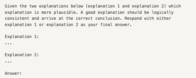### A.4 LLM-as-a-Judge Baseline <details> <summary>extracted/6246183/llm-judge-prompt.png Details</summary>  ### Visual Description ## Screenshot: Evaluation Prompt Template ### Overview The image is a screenshot of a text-based prompt or template. It presents instructions for evaluating two hypothetical explanations ("Explanation 1" and "Explanation 2") and selecting the more plausible one based on logical consistency and correctness. The text is presented in a monospaced font on a light gray background, suggesting it may be from a code editor, terminal, or a plain text document. ### Components / Text Content The image contains the following text, transcribed verbatim: ``` Given the two explanations below (explanation 1 and explanation 2) which explanation is more plausible. A good explanation should be logically consistent and arrive at the correct conclusion. Respond with either explanation 1 or explanation 2 as your final answer. Explanation 1: ... Explanation 2: ... Answer: ``` **Spatial Layout:** - The main instruction paragraph is at the top. - Below it, the labels "Explanation 1:" and "Explanation 2:" are listed vertically, each followed by an ellipsis (`...`) on the next line, indicating placeholder content. - At the bottom, the label "Answer:" is present, also followed by a placeholder. ### Detailed Analysis / Content Details - **Instruction Text:** The core directive is to compare two explanations for plausibility. The criteria for a "good explanation" are explicitly defined as being "logically consistent" and arriving at the "correct conclusion." - **Structure:** The template is designed for a binary choice. The respondent is instructed to output either "explanation 1" or "explanation 2" as the final answer. - **Placeholders:** The ellipses (`...`) under each explanation label signify that the actual content of the explanations is not provided in this image. This image is a shell or a prompt awaiting input. ### Key Observations - The text is purely instructional and contains no data, charts, or diagrams. - The language is precise and task-oriented, focusing on logical evaluation. - The format is minimal and functional, with clear separation between the instruction, the input fields (for the explanations), and the output field (for the answer). ### Interpretation This image does not contain factual data or a completed analysis. Instead, it represents a **meta-instruction** or a **prompt template**. Its purpose is to structure a reasoning task. 1. **Function:** It serves as a framework for an exercise in critical thinking or argument evaluation. The user (or an AI system) would be expected to populate "Explanation 1" and "Explanation 2" with specific arguments and then apply the given criteria to choose between them. 2. **Implied Context:** This template could be used in various contexts, such as: * An educational setting for teaching logical reasoning. * A testing or benchmarking scenario for AI models, evaluating their ability to assess argument quality. * A step in a larger problem-solving workflow where multiple solution paths are compared. 3. **Underlying Principle:** The prompt enforces a clear, two-part standard for evaluation: internal coherence (logical consistency) and external validity (correctness of the conclusion). This moves beyond subjective preference to an objective, rule-based assessment. In essence, the image provides the *scaffolding for a judgment call*, not the judgment itself. The actual informational content to be processed is absent, indicated by the placeholders. </details> Figure 10: An example of prompt used by the LLM-as-a-Judge model for evaluating competing explanations. GPT 3.5 is used as the LLM for the LLM-as-a-Judge baseline. Similar to the human evaluators, GPT is presented with both generated explanations and asked to identify which explanation is more plausible. 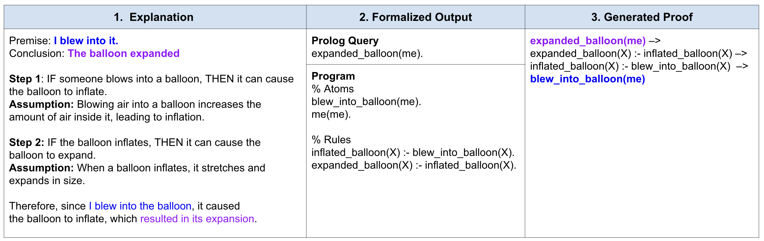### A.5 Logical Consistency <details> <summary>extracted/6246183/logical-pipeline.png Details</summary>  ### Visual Description ## Table: Logical Reasoning Formalization Example ### Overview The image displays a three-column table that illustrates the process of translating a simple natural language causal argument into a formal logic program (Prolog) and its corresponding proof chain. The example uses the scenario of blowing into a balloon causing it to expand. ### Components/Axes The table is structured with three vertical columns, each with a distinct header: 1. **Column 1 Header (Top-Left):** "1. Explanation" 2. **Column 2 Header (Top-Center):** "2. Formalized Output" 3. **Column 3 Header (Top-Right):** "3. Generated Proof" The table has a light blue header row and white body cells with black borders. ### Detailed Analysis / Content Details **Column 1: Explanation** This column contains the natural language reasoning. * **Premise:** "I blew into it." (The phrase "I blew into it" is in **blue** text). * **Conclusion:** "The balloon expanded" (The phrase "The balloon expanded" is in **purple** text). * **Step 1:** "IF someone blows into a balloon, THEN it can cause the balloon to inflate." * **Assumption:** "Blowing air into a balloon increases the amount of air inside it, leading to inflation." * **Step 2:** "IF the balloon inflates, THEN it can cause the balloon to expand." * **Assumption:** "When a balloon inflates, it stretches and expands in size." * **Final Statement:** "Therefore, since I blew into the balloon, it caused the balloon to inflate, which resulted in its expansion." (Within this sentence, "I blew into the balloon" is in **blue** text, and "resulted in its expansion" is in **purple** text). **Column 2: Formalized Output** This column contains the corresponding Prolog program code. * **Section Header:** "Prolog Query" * Code: `expanded_balloon(me).` * **Section Header:** "Program" * Subsection: "% Atoms" * Code: `blew_into_balloon(me).` * Code: `me(me).` * Subsection: "% Rules" * Code: `inflated_balloon(X) :- blew_into_balloon(X).` * Code: `expanded_balloon(X) :- inflated_balloon(X).` **Column 3: Generated Proof** This column shows the logical proof chain derived from the program, using color-coding that matches the Explanation column. * Line 1: `expanded_balloon(me) →` (The predicate `expanded_balloon(me)` is in **purple** text). * Line 2: `expanded_balloon(X) :- inflated_balloon(X) →` * Line 3: `inflated_balloon(X) :- blew_into_balloon(X) →` * Line 4: `blew_into_balloon(me)` (The predicate `blew_into_balloon(me)` is in **blue** text). ### Key Observations 1. **Color-Coding Consistency:** There is a strict visual link between the natural language elements and their formal counterparts. The blue text for the initial action ("I blew into it" / `blew_into_balloon(me)`) and the purple text for the final outcome ("The balloon expanded" / `expanded_balloon(me)`) is maintained across columns 1 and 3. 2. **Structural Mapping:** The table demonstrates a clear, stepwise transformation: * **Column 1** provides the intuitive, assumption-laden human reasoning. * **Column 2** strips away the assumptions and translates the core causal rules and facts into a formal, machine-readable syntax (Prolog). * **Column 3** shows the backward-chaining proof process the Prolog engine would use to derive the conclusion from the initial query and rules. 3. **Logical Flow:** The proof in Column 3 reads from top to bottom as a goal-directed search: to prove `expanded_balloon(me)`, it needs `inflated_balloon(me)`, which in turn requires `blew_into_balloon(me)`, which is a known fact. ### Interpretation This table serves as a pedagogical or demonstrative tool for symbolic AI and logic programming. It bridges the gap between human-understandable causal reasoning and formal logical representation. * **What it demonstrates:** It shows how a simple cause-and-effect narrative can be decomposed into atomic facts (`me(me)`, `blew_into_balloon(me)`) and general rules (`inflated_balloon(X) :- ...`). The "Assumptions" in Column 1 are the real-world knowledge that is implicitly encoded into the structure of the rules in Column 2 (e.g., the rule `inflated_balloon(X) :- blew_into_balloon(X).` encapsulates the assumption that blowing causes inflation). * **Relationship between elements:** The columns represent different "languages" for the same knowledge: natural language, Prolog code, and a proof trace. The color-coding acts as a crucial cross-reference, grounding the abstract symbols (`me`, `blew_into_balloon`) back to the concrete scenario. * **Underlying purpose:** The image likely aims to explain the process of "formalization" – how to convert vague, context-rich human statements into precise, unambiguous logical statements that a computer can process to derive conclusions reliably. It highlights the power and clarity of logic programming for representing and reasoning about simple causal chains. </details> Figure 11: An example of the autoformalization prompt. An explanation hypothesis is considered logically consistent if the external solver can build a deductive proof connecting the conclusion to the premise. We use NLProlog Weber et al. (2019), a neuro-symbolic Prolog solver integrating backward chaining with word embedding models via a weak unification mechanism. NLProlog allows for a level of flexibility and robustness that is necessary for NLP use cases (e.g. unification applied to synonyms). We provide the autoformalized query, atoms, and rules to NLProlog. If NLProlog can satisfy the entailment query, it will return the proof consisting of the set of rules traversed, the weak unification score, and the proof depth. For simplicity, we assign a score of one if the entailment query is satisfied and zero if it is not. The proof depth score is evaluated as part of the parsimony analysis. An end-to-end example of consistency evaluation can be found in Figure 11. 1 Input : Symbolic KB $kb$ , Goal $goal$ , Glove embedding model $e(\cdot)$ Output : proof chain $chain$ , proof depth $depth$ 2 3 threshold $\leftarrow$ 0.13; 4 5 $depth$ $\leftarrow$ 1 ; 6 $chain$ $\leftarrow$ $emptylist$ ; 7 8 foreach step $t$ in backward_chaining( $kb$ , $goal$ ) do 9 foreach $max\_unification(q,q_{t})$ do 10 $unification\_score$ $\leftarrow$ $CosineSimilarity$ ( $e(q,m_{s}),e(q_{t},m_{s})$ ); 11 $depth$ $\leftarrow$ $depth$ $\times$ $unification\_score$ ; 12 13 end foreach 14 $chain$ $\leftarrow$ backward_chaining( $kb$ , $goal$ ); 15 16 end foreach 17 18 if $chain$ is not empty and $depth$ $>$ threshold then 19 $chain\leftarrow$ current_proof_chain $[0]$ ; 20 21 end if 22 else 23 $depth$ $\leftarrow$ 0 ; 24 end if 25 26 return $chain$ , $depth$ ; Algorithm 1 Neuro-symbolic Solver ### A.6 Parsimony Parsimony measures the complexity of an explanation and is represented by the proof depth and concept drift metrics. Proof depth is automatically calculated by NLProlog and reflects the number of rules traversed by the solver to satisfy the entailment query. If the hypothesis is not logically consistent, depth is set to zero. The concept drift metric measures the entropy of novel concepts introduced to bridge the premise and conclusion. To compute the drift of an explanation, we consider the nouns found in the premise, conclusion, and explanation steps. We use Spacy Honnibal and Montani (2017) to tokenize and extract part-of-speech (POS) tags. All tokens with the ’NOUN’ POS tag extracted. For normalization purposes, we consider the lemma of the tokens. Concept drift then is calculated as the set difference between the unique nouns found across all explanation steps and those found in the premise and conclusion. 1 2 Input : Premise, Conclusion, Explanation, Spacy model $spacy$ ( $\cdot$ ) Output : Drift Score $drift$ 3 4 $Noun_{p}\leftarrow$ $spacy$ ( $Premise$ ); 5 $Noun_{c}\leftarrow$ $spacy$ ( $Conclusion$ ); 6 $Noun_{E}\leftarrow$ $spacy$ ( $Explanation$ ); 7 $N\leftarrow\{Noun_{p},Noun_{c},Noun_{E}\}$ ; 8 $drift\leftarrow length(set(Noun_{E})-set(Noun_{p}\cup Noun_{c})$ ); 9 return $drift$ ; Algorithm 2 Concept Drift ### A.7 Coherence Coherence evaluates the plausibility of the intermediate explanation. We propose stepwise entailment as a metric to measure the entailment strength of the If-then implications. We employ a RoBERTa-based NLI model Nie et al. (2020) that has been finetuned on a range of NLI and fact verification datasets consisting of SNLI Bowman et al. (2015), aNLI Nie et al. (2020), multilingual NLI Williams et al. (2018)), and FEVER-NLI Nie et al. (2019). To compute the stepwise entailment score, we first measure the entailment strength between the If and Then propositions. For example, to calculate the score of the statement “IF a balloon is pricked, THEN the balloon may deflate” we consider “a balloon is pricked” and “the balloon may deflate” as input sentences for the NLI model. The NLI will produce independent scores for the entailment and contradiction labels. We compute the entailment strength by subtracting the contraction label score from the entailment label score. An entailment strength of one indicates the If-then implication is strongly plausible whereas a score of zero suggests that it is likely implausible. The overall stepwise entailment score is the average of entailment strength measures across all explanation steps. 1 2 Input : Explanation $E$ , NLI Model $nli$ ( $\cdot$ ) Output : Average Entailment Strength $strength$ 3 4 $EntailmentStrengthScores\leftarrow$ empty list; 5 6 foreach Step $(If_{s},Then_{s})$ in $E$ do 7 $EntailmentScore\leftarrow$ $nli$ ( $If_{s}$ , $Then_{s}$ ); 8 $ContradictionScore\leftarrow$ $nli$ ( $If_{s}$ , $Then_{s}$ ); 9 $EntailmentStrength\leftarrow EntailmentScore-ContradictionScore$ ; 10 Append $EntailmentStrength$ to $EntailmentStrengthScores$ ; 11 12 end foreach 13 14 $strength\leftarrow$ $Avg$ ( $EntailmentStrengthScores$ ); 15 return $strength$ ; Algorithm 3 Stepwise Entailment ### A.8 Linguistic Uncertainty Linguistic uncertainty measures the confidence of a statement where hedging cues and indirect language suggest ambiguity around the proposition. To measure sentence-level uncertainty, we employ a finetuned RoBERTa model provided by Pei and Jurgens (2021). The model was trained on a sentence-level dataset consisting of findings and statements extracted from new articles and scientific publications and human annotated evaluation of sentence certainty. A scale from one to six was used to annotate sentences where one corresponds to the lowest degree of certainty and six is the highest expressed by the sentence. We invert the scale to retrieve the uncertainty scores. To compute the overall linguistic uncertainty of an explanation, we first compute the uncertainty for each assumption and the explanation summary and then average all the scores. We use a fine-tuned BERT-based token classification model to classify all the words in the generated explanation with uncertainty categories introduced in the 2010 CoNLL shared task on Hedge Detection Farkas et al. (2010). Farkas et al. (2010) classify hedge cues into three categories: epistemic, doxatic, and conditional. Epistemic cues refer to hedging scenarios where the truth value of a proposition can be determined but is unknown in the present (e.g. the blocks may fall). Doxatic cues refer to beliefs and hypotheses that can be held to be true or false by others (e.g. the child believed the blocks would fall). Finally, conditional cues refer to propositions whose truth value is dependent on another proposition’s truth value (e.g. if the balloon is pricked it may deflate). 1 2 Input : Assumptions, Explanation Summary, Uncertainty Estimator Model $uc(\cdot)$ Output : Overall Uncertainty 3 4 $AssumptionUncertaintyList\leftarrow$ empty list; 5 6 foreach Assumption in Assumptions do 7 $UncertaintyScore\leftarrow$ $uc$ ( $UncertaintyModel$ , $Assumption$ ); 8 Append $UncertaintyScore$ to $AssumptionUncertaintyList$ ; 9 10 end foreach 11 12 $AverageAssumptionUncertainty\leftarrow$ $Avg$ ( $AssumptionUncertaintyList$ ); 13 14 $ExplanationUncertainty\leftarrow$ $uc$ ( $UncertaintyModel$ , $ExplanationSummary$ ); 15 16 $OverallExplanationUncertainty\leftarrow AverageAssumptionUncertainty+ExplanationUncertainty$ ; 17 18 return $OverallExplanationUncertainty$ ; Algorithm 4 Linguistic Uncertainty ### A.9 Inference to Best Explanation To perform IBE, we first fit a linear regression model over the extracted explanation features from the COPA train set and 500 random sample train examples from the E-CARE train set. We consider all explanations independently and annotate each explanation with a 1 if it corresponds to a correct answer or 0 if corresponds to an incorrect answer. After the linear model is fitted, we evaluate the COPA and E-CARE test sets. For each example, we use the trained linear model to score each answer candidate explanation and then select a candidate with the highest score. We use the linear regression implementation from scikit-learn Buitinck et al. (2013) for the IBE model. We additionally use the R stats package R Core Team (2013) for conducting our regression analysis. ### A.10 E-CARE Results #### A.10.1 E-CARE Consistency See Figure 12. 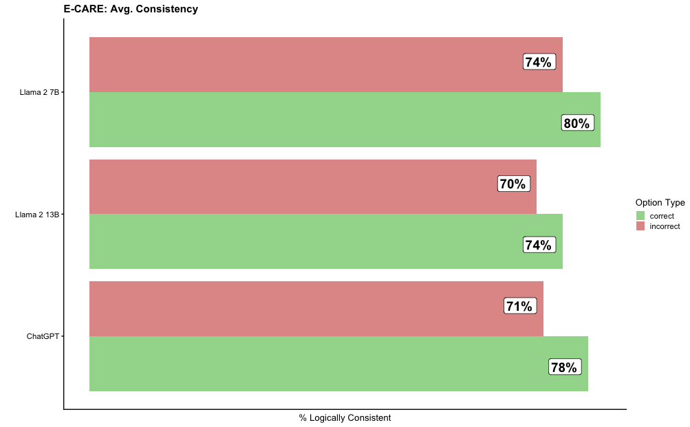<details> <summary>extracted/6246183/consistency-ecare.png Details</summary>  ### Visual Description \n ## Horizontal Bar Chart: E-CARE: Avg. Consistency ### Overview This is a horizontal bar chart comparing the average logical consistency percentages of three large language models (LLMs) on the E-CARE benchmark. The chart evaluates each model's performance on "correct" versus "incorrect" option types. ### Components/Axes * **Chart Title:** "E-CARE: Avg. Consistency" (located at the top-left). * **Y-Axis (Vertical):** Lists the three models being compared. From top to bottom: "Llama 2 7B", "Llama 2 13B", "ChatGPT". * **X-Axis (Horizontal):** Labeled "% Logically Consistent". The axis scale runs from 0 to 100, with major tick marks at 0, 20, 40, 60, 80, and 100. * **Legend:** Located on the right side of the chart, titled "Option Type". It defines two categories: * A green square labeled "correct". * A red (salmon/pinkish-red) square labeled "incorrect". * **Data Bars:** For each model, there are two horizontal bars stacked vertically. The top bar for each model is red (incorrect), and the bottom bar is green (correct). Each bar has its exact percentage value annotated at its right end. ### Detailed Analysis The chart presents the following specific data points, confirmed by cross-referencing bar color with the legend: **1. Llama 2 7B (Topmost model group)** * **Incorrect (Red Bar):** 74% * **Correct (Green Bar):** 80% * **Trend:** The green "correct" bar is longer than the red "incorrect" bar, indicating higher consistency for correct options. **2. Llama 2 13B (Middle model group)** * **Incorrect (Red Bar):** 70% * **Correct (Green Bar):** 74% * **Trend:** The green "correct" bar is longer than the red "incorrect" bar. Both values are lower than the corresponding values for Llama 2 7B. **3. ChatGPT (Bottom model group)** * **Incorrect (Red Bar):** 71% * **Correct (Green Bar):** 78% * **Trend:** The green "correct" bar is longer than the red "incorrect" bar. Its "correct" score is the second highest, and its "incorrect" score is the second lowest among the three models. ### Key Observations * **Universal Pattern:** For all three models, the logical consistency score for "correct" options is higher than for "incorrect" options. * **Highest Score:** Llama 2 7B achieves the highest single score on the chart: 80% consistency on correct options. * **Lowest Score:** Llama 2 13B has the lowest score on the chart: 70% consistency on incorrect options. * **Model Comparison:** Llama 2 7B outperforms Llama 2 13B on both metrics. ChatGPT's performance falls between the two Llama models on the "correct" metric but is closer to Llama 2 13B on the "incorrect" metric. * **Consistency Gap:** The gap between "correct" and "incorrect" consistency is largest for ChatGPT (7 percentage points) and smallest for Llama 2 13B (4 percentage points). ### Interpretation This chart from the E-CARE benchmark suggests a fundamental characteristic of the evaluated LLMs: they are more logically consistent when generating or evaluating correct answers compared to incorrect ones. This could imply that the models' reasoning processes are more robust or less prone to contradiction when aligned with factual or logically sound premises. The data does not show a simple "bigger model is better" trend, as the smaller Llama 2 7B model outperforms the larger Llama 2 13B model on both measures. This could point to factors beyond parameter count, such as differences in training data, fine-tuning, or the specific nature of the E-CARE tasks. ChatGPT demonstrates strong but not leading performance, sitting between the two Llama variants. The relatively narrow range of scores (70% to 80%) indicates that all models achieve a moderately high level of logical consistency on this benchmark, but there is clear room for improvement, especially on handling incorrect options consistently. </details> Figure 12: Average consistency comparison between correct and incorrect options for the E-CARE dataset. #### A.10.2 E-CARE Proof Depth See Figure 13. 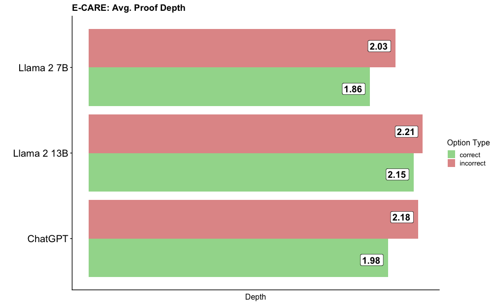<details> <summary>extracted/6246183/depth-ecare.png Details</summary>  ### Visual Description ## Horizontal Bar Chart: E-CARE: Avg. Proof Depth ### Overview The image displays a horizontal bar chart titled "E-CARE: Avg. Proof Depth." It compares the average proof depth metric for three different large language models (LLMs) when generating correct versus incorrect answers. The chart uses paired bars for each model, with green representing "correct" options and red representing "incorrect" options. ### Components/Axes * **Chart Title:** "E-CARE: Avg. Proof Depth" (located at the top-left). * **Y-Axis (Vertical):** Lists the three models being compared. From top to bottom: * Llama 2 7B * Llama 2 13B * ChatGPT * **X-Axis (Horizontal):** Labeled "Depth" at the bottom. The axis represents a numerical scale for average proof depth, though specific tick marks are not shown. The values are provided as data labels on the bars. * **Legend:** Located on the right side of the chart, titled "Option Type." * A green square corresponds to "correct." * A red square corresponds to "incorrect." * **Data Labels:** Each bar has a numerical value displayed at its end, indicating the precise average proof depth. ### Detailed Analysis The chart presents the following data points for each model: 1. **Llama 2 7B:** * **Correct (Green Bar):** Average proof depth = 1.86. The green bar is shorter than the red bar for this model. * **Incorrect (Red Bar):** Average proof depth = 2.03. The red bar is longer than the green bar. 2. **Llama 2 13B:** * **Correct (Green Bar):** Average proof depth = 2.15. The green bar is shorter than the red bar. * **Incorrect (Red Bar):** Average proof depth = 2.21. The red bar is longer than the green bar. 3. **ChatGPT:** * **Correct (Green Bar):** Average proof depth = 1.98. The green bar is shorter than the red bar. * **Incorrect (Red Bar):** Average proof depth = 2.18. The red bar is longer than the green bar. **Trend Verification:** For all three models (Llama 2 7B, Llama 2 13B, and ChatGPT), the visual trend is consistent: the red bar (incorrect) is always longer than the green bar (correct). This indicates a higher average proof depth for incorrect answers across the board. ### Key Observations * **Consistent Pattern:** The most notable pattern is that for every model listed, the average proof depth for incorrect answers is higher than for correct answers. * **Model Comparison:** * Llama 2 13B shows the highest average proof depth values for both correct (2.15) and incorrect (2.21) options among the three models. * Llama 2 7B shows the lowest average proof depth for correct options (1.86). * The difference between incorrect and correct proof depth is smallest for Llama 2 13B (0.06) and largest for ChatGPT (0.20). * **Value Range:** All extracted average proof depth values fall within a relatively narrow range, between 1.86 and 2.21. ### Interpretation The data suggests a potential correlation between the complexity or length of the reasoning chain (as measured by "proof depth") and the correctness of the model's output. Specifically, **incorrect answers tend to be associated with longer, more complex proof chains** than correct answers for these models on the E-CARE benchmark. This could imply several investigative possibilities: 1. **Overthinking/Confabulation:** Models may generate longer, more convoluted justifications when they are uncertain or "hallucinating," leading to incorrect conclusions. 2. **Error Propagation:** A longer chain of reasoning provides more opportunities for a logical error to occur, which could result in an incorrect final answer. 3. **Task Difficulty:** Questions that elicit incorrect answers might inherently be more difficult, prompting the model to attempt a longer, but ultimately flawed, reasoning process. The fact that this pattern holds across three different models (including two sizes of Llama 2 and ChatGPT) suggests it may be a general characteristic of how these LLMs perform on this type of reasoning task, rather than an artifact of a single model's architecture. The metric "proof depth" itself is central to this analysis, likely counting the number of logical steps or inferences in a generated explanation. </details> Figure 13: Comparison of average proof depth between correct and incorrect options. 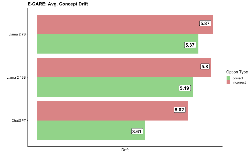<details> <summary>extracted/6246183/drift-ecare.png Details</summary>  ### Visual Description ## Horizontal Bar Chart: E-CARE: Avg. Concept Drift ### Overview The image displays a horizontal bar chart titled "E-CARE: Avg. Concept Drift." It compares the average concept drift metric for three different large language models (LLMs) across two categories: "correct" and "incorrect" option types. The chart suggests that for all models, the average drift is higher when the model's output is incorrect compared to when it is correct. ### Components/Axes * **Chart Title:** "E-CARE: Avg. Concept Drift" (located at the top-left). * **Y-Axis (Vertical):** Lists the three models being compared. From top to bottom: 1. Llama 2 7B 2. Llama 2 13B 3. ChatGPT * **X-Axis (Horizontal):** Labeled "Drift" at the bottom center. The axis represents a numerical scale for the drift metric, though specific tick marks are not shown. The values are provided as data labels on the bars. * **Legend:** Positioned on the right side of the chart, titled "Option Type." * A green square corresponds to the label "correct." * A red (salmon) square corresponds to the label "incorrect." * **Data Bars:** For each model, there are two horizontal bars: * A green bar representing the "correct" option type. * A red (salmon) bar representing the "incorrect" option type. * Each bar has a numerical value displayed at its right end. ### Detailed Analysis **Data Points and Trends:** The chart presents the following specific values for average concept drift: | Model | Incorrect Drift (Red Bar) | Correct Drift (Green Bar) | Trend | | :--- | :--- | :--- | :--- | | **Llama 2 7B** | 5.87 | 5.37 | The red bar is longer than the green bar, indicating higher drift for incorrect outputs. | | **Llama 2 13B** | 5.8 | 5.19 | The red bar is longer than the green bar, indicating higher drift for incorrect outputs. | | **ChatGPT** | 5.02 | 3.61 | The red bar is significantly longer than the green bar, indicating a much higher drift for incorrect outputs. | **Visual Trend Verification:** * For all three models, the "incorrect" (red) bar extends further to the right than its corresponding "correct" (green) bar. This visually confirms the trend that average concept drift is consistently higher for incorrect responses. * The gap between the red and green bars appears largest for ChatGPT and smallest for Llama 2 7B. ### Key Observations 1. **Consistent Pattern:** Across all three models, the average concept drift metric is higher for incorrect option types than for correct ones. 2. **Model Comparison:** * **Highest Drift (Incorrect):** Llama 2 7B has the highest recorded drift value at 5.87. * **Lowest Drift (Correct):** ChatGPT has the lowest recorded drift value at 3.61. * **Largest Discrepancy:** ChatGPT shows the greatest difference between its incorrect (5.02) and correct (3.61) drift scores, a difference of approximately 1.41. * **Smallest Discrepancy:** Llama 2 7B shows the smallest difference between its incorrect (5.87) and correct (5.37) drift scores, a difference of 0.50. 3. **Model Size Trend (Llama 2):** Between the two Llama 2 models, the larger 13B model shows slightly lower drift values for both correct (5.19 vs. 5.37) and incorrect (5.8 vs. 5.87) categories compared to the smaller 7B model. ### Interpretation The data suggests a strong correlation between a model's correctness on a task (as defined by the E-CARE benchmark) and its measured "concept drift." Concept drift, in this context, likely refers to a shift or instability in the model's internal representations or reasoning process. * **Higher Drift for Errors:** The consistent finding that drift is higher for incorrect outputs implies that when a model makes a mistake, its internal processing may be less stable or more divergent from a consistent conceptual pathway. Correct answers appear to be associated with more stable internal states. * **ChatGPT's Profile:** ChatGPT exhibits the most stable performance (lowest drift) when correct, but its drift increases substantially when incorrect. This could indicate that its correct reasoning is highly consistent, but its failure modes involve a more significant breakdown in conceptual stability. * **Llama 2 Stability:** The Llama 2 models show higher baseline drift even when correct, and the increase when incorrect is less dramatic. This might suggest a different internal architecture or training paradigm that results in a different drift profile, potentially with more inherent variability in its representations. * **Implication for Reliability:** If "concept drift" is a proxy for reasoning reliability, this chart indicates that monitoring drift could be a potential method for detecting when a model is likely to be incorrect. The clear separation between correct and incorrect drift values for each model supports this idea. **Note on Language:** All text in the image is in English. </details> Figure 14: Comparison of average concept drift between correct and incorrect options. 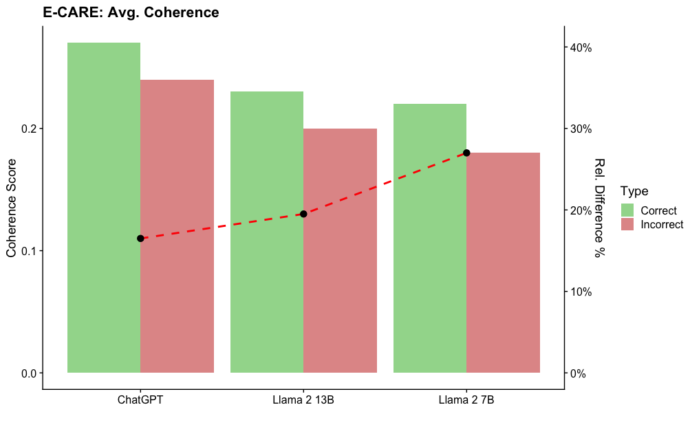<details> <summary>extracted/6246183/coherence-ecare.png Details</summary>  ### Visual Description ## Bar Chart with Line Overlay: E-CARE: Avg. Coherence ### Overview The image is a combination bar and line chart titled "E-CARE: Avg. Coherence". It compares the average coherence scores for "Correct" and "Incorrect" responses across three different large language models: ChatGPT, Llama 2 13B, and Llama 2 7B. A secondary axis shows the relative percentage difference between the correct and incorrect scores for each model. ### Components/Axes * **Title:** "E-CARE: Avg. Coherence" (Top-left, bold). * **Primary Y-Axis (Left):** Labeled "Coherence Score". Scale ranges from 0.0 to just above 0.2, with major ticks at 0.0, 0.1, and 0.2. * **Secondary Y-Axis (Right):** Labeled "Rel. Difference %". Scale ranges from 0% to 40%, with major ticks at 0%, 10%, 20%, 30%, and 40%. * **X-Axis:** Lists three model names: "ChatGPT", "Llama 2 13B", and "Llama 2 7B". * **Legend:** Positioned on the right side, between the two y-axes. It defines the bar colors under the header "Type": * Green square: "Correct" * Red square: "Incorrect" * **Data Series:** 1. **Bar Series (Correct):** Light green bars. 2. **Bar Series (Incorrect):** Light red/salmon bars. 3. **Line Series:** A red dashed line with black circular markers at each data point, corresponding to the right y-axis ("Rel. Difference %"). ### Detailed Analysis **Bar Data (Coherence Score - Left Axis):** * **ChatGPT:** * Correct (Green Bar): Approximately 0.24. * Incorrect (Red Bar): Approximately 0.22. * **Llama 2 13B:** * Correct (Green Bar): Approximately 0.22. * Incorrect (Red Bar): Approximately 0.20. * **Llama 2 7B:** * Correct (Green Bar): Approximately 0.21. * Incorrect (Red Bar): Approximately 0.18. **Line Data (Relative Difference % - Right Axis):** The red dashed line shows an upward trend from left to right. * **ChatGPT:** The black dot aligns with approximately 17% on the right axis. * **Llama 2 13B:** The black dot aligns with approximately 19% on the right axis. * **Llama 2 7B:** The black dot aligns with approximately 28% on the right axis. **Trend Verification:** * For all three models, the green "Correct" bar is taller than the red "Incorrect" bar, indicating higher coherence scores for correct answers. * The height of both the green and red bars decreases progressively from ChatGPT to Llama 2 13B to Llama 2 7B. * The red dashed line (Relative Difference) slopes upward, indicating the percentage gap between correct and incorrect coherence scores increases as we move from ChatGPT to the smaller Llama models. ### Key Observations 1. **Consistent Performance Gap:** Every model exhibits a higher average coherence score for its correct responses compared to its incorrect ones. 2. **Model Size Correlation:** There is a visible trend where the absolute coherence scores (for both correct and incorrect) are highest for ChatGPT, lower for Llama 2 13B, and lowest for Llama 2 7B. 3. **Increasing Disparity:** The relative difference (gap) between correct and incorrect coherence is smallest for ChatGPT (~17%) and largest for Llama 2 7B (~28%). This suggests the performance disparity grows as model size decreases within the Llama 2 family. 4. **Visual Layout:** The legend is placed in the right margin. The bars are grouped by model, with the "Correct" bar always to the left of the "Incorrect" bar for each model. The line chart is overlaid on the bar chart, with its markers centered over each model group. ### Interpretation This chart from the E-CARE benchmark suggests a relationship between a model's overall capability and the consistency of its output coherence. Larger or more capable models (like ChatGPT in this comparison) not only achieve higher absolute coherence scores but also maintain a more consistent level of coherence between their correct and incorrect answers. The increasing relative difference for smaller models (Llama 2 13B and 7B) indicates that when these models make errors, the coherence of their reasoning or output degrades more sharply compared to their correct responses. This could imply that model scale contributes to more robust and stable generation quality, even in failure modes. The data highlights that evaluating models on correct answers alone may not capture the full picture of their reliability; the quality of their errors is also a critical metric. </details> Figure 15: Comparison of average coherence scores between correct and incorrect options. 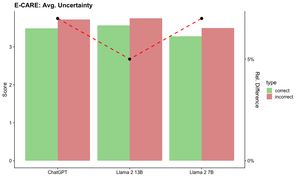<details> <summary>extracted/6246183/uncertainty-ecare.png Details</summary>  ### Visual Description \n ## Bar Chart with Line Overlay: E-CARE: Avg. Uncertainty ### Overview This is a grouped bar chart with a secondary axis line overlay. It compares the average uncertainty scores for correct versus incorrect responses across three different AI models: ChatGPT, Llama 2 13B, and Llama 2 7B. A dashed red line plots the relative percentage difference between the incorrect and correct scores for each model. ### Components/Axes * **Title:** "E-CARE: Avg. Uncertainty" (Top-left corner). * **Primary Y-Axis (Left):** * **Label:** "Score" * **Scale:** Linear, from 0 to 3, with major ticks at 0, 1, 2, 3. * **Secondary Y-Axis (Right):** * **Label:** "Rel. Difference" * **Scale:** Percentage, from 0% to 5%, with major ticks at 0% and 5%. * **X-Axis:** * **Categories (from left to right):** "ChatGPT", "Llama 2 13B", "Llama 2 7B". * **Legend (Centered on the right side):** * **Title:** "type" * **Green square:** "correct" * **Red square:** "incorrect" * **Data Series:** 1. **Grouped Bars:** Two bars per x-axis category. * Left bar (Green): Represents the average uncertainty score for "correct" responses. * Right bar (Red): Represents the average uncertainty score for "incorrect" responses. 2. **Line Overlay:** A red dashed line connecting black circular data points. Each point is positioned above its corresponding model group and corresponds to the "Rel. Difference" (right y-axis). ### Detailed Analysis **Bar Values (Approximate Scores from Left Y-Axis):** * **ChatGPT:** * Correct (Green): ~3.5 * Incorrect (Red): ~3.7 * **Llama 2 13B:** * Correct (Green): ~3.6 * Incorrect (Red): ~3.8 * **Llama 2 7B:** * Correct (Green): ~3.3 * Incorrect (Red): ~3.5 **Line Data Points (Approximate Relative Difference from Right Y-Axis):** * **ChatGPT:** The black dot is positioned slightly above the 5% tick mark, at approximately **5.5%**. * **Llama 2 13B:** The black dot is positioned below the 5% tick mark, at approximately **4.5%**. * **Llama 2 7B:** The black dot is positioned slightly above the 5% tick mark, at approximately **5.5%**. **Trend Verification:** * **Bar Trend:** For all three models, the red bar (incorrect) is taller than the green bar (correct), indicating higher average uncertainty scores for incorrect answers. * **Line Trend:** The red dashed line starts high for ChatGPT (~5.5%), dips to its lowest point for Llama 2 13B (~4.5%), and rises back to a similar high level for Llama 2 7B (~5.5%). This creates a shallow "V" shape. ### Key Observations 1. **Consistent Pattern:** Across all models, incorrect responses are associated with higher measured uncertainty than correct responses. 2. **Model Comparison:** Llama 2 13B shows the smallest relative difference (~4.5%) between correct and incorrect uncertainty scores, while ChatGPT and Llama 2 7B show a larger, nearly identical difference (~5.5%). 3. **Absolute Scores:** The absolute uncertainty scores (left axis) are relatively high (all above 3 on a scale that appears to max at or above 3.8) and vary less between models than the relative difference does. 4. **Visual Emphasis:** The chart uses a dual-axis design to simultaneously show absolute values (bars) and a derived comparative metric (line), highlighting the relationship between the two. ### Interpretation The data suggests a strong correlation between a model's expressed uncertainty (as measured by the E-CARE metric) and the correctness of its output. Higher uncertainty scores are a reliable indicator of potential incorrectness across these models. The **relative difference** metric (the line) provides a normalized view of this gap. The fact that Llama 2 13B has a smaller relative difference could imply one of two things, or a combination: 1. **Better Calibration:** Its uncertainty estimates might be more finely tuned, making the distinction between correct and incorrect states less dramatic in terms of raw score. 2. **Different Operating Range:** Its overall uncertainty scores might be shifted, making the absolute gap similar but the percentage difference smaller. The nearly identical relative difference for ChatGPT and Llama 2 7B, despite potential differences in their architecture and training, suggests this ~5.5% gap might be a common characteristic or a benchmark result for this type of evaluation. The chart effectively argues that monitoring model uncertainty is a valuable signal for assessing answer reliability, with the specific magnitude of the signal varying by model. </details> Figure 16: Comparison of average uncertainty scores between correct and incorrect options. 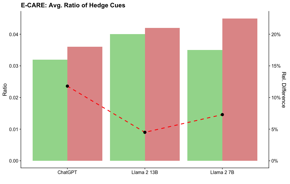<details> <summary>extracted/6246183/hedge-ratio-ecare.png Details</summary>  ### Visual Description \n ## Bar Chart with Line Overlay: E-CARE: Avg. Ratio of Hedge Cues ### Overview This is a dual-axis combination chart comparing the average ratio of "Hedge Cues" across three large language models: ChatGPT, Llama 2 13B, and Llama 2 7B. The chart uses grouped bars to display two distinct ratios for each model and a dashed line to show the relative difference between them. ### Components/Axes * **Title:** "E-CARE: Avg. Ratio of Hedge Cues" (Top-left, bold). * **X-Axis (Categorical):** Lists three models: "ChatGPT", "Llama 2 13B", "Llama 2 7B". * **Primary Y-Axis (Left):** Labeled "Ratio". Scale ranges from 0.00 to 0.04, with major ticks at 0.00, 0.01, 0.02, 0.03, and 0.04. * **Secondary Y-Axis (Right):** Labeled "Rel. Difference". Scale is in percentages, ranging from 0% to 20%, with major ticks at 0%, 5%, 10%, 15%, and 20%. * **Data Series (Bars):** Two bars per model. * **Green Bar (Left bar in each group):** Represents one category of hedge cue ratio (e.g., perhaps "Hedge Cues" or a specific type). * **Red Bar (Right bar in each group):** Represents a second, contrasting category of hedge cue ratio (e.g., perhaps "Non-Hedge Cues" or a different type). * *Note: The specific legend defining the green and red categories is not present within the chart area.* * **Data Series (Line):** A red dashed line with black circular markers at each data point, plotted against the right "Rel. Difference" axis. ### Detailed Analysis **Bar Data (Approximate Values from Left "Ratio" Axis):** 1. **ChatGPT:** * Green Bar: ~0.032 * Red Bar: ~0.036 2. **Llama 2 13B:** * Green Bar: ~0.040 * Red Bar: ~0.042 3. **Llama 2 7B:** * Green Bar: ~0.035 * Red Bar: ~0.045 **Line Data (Approximate Values from Right "Rel. Difference" Axis):** * The red dashed line connects three black data points. * **Point 1 (Above ChatGPT):** ~12% * **Point 2 (Above Llama 2 13B):** ~5% * **Point 3 (Above Llama 2 7B):** ~7% **Trend Verification:** * **Green Bar Trend:** The ratio increases from ChatGPT (~0.032) to Llama 2 13B (~0.040), then decreases for Llama 2 7B (~0.035). * **Red Bar Trend:** The ratio shows a steady increase from ChatGPT (~0.036) to Llama 2 13B (~0.042) to Llama 2 7B (~0.045). * **Line Trend (Rel. Difference):** The relative difference starts at ~12% for ChatGPT, drops sharply to its lowest point at ~5% for Llama 2 13B, and then rises slightly to ~7% for Llama 2 7B. ### Key Observations 1. For all three models, the value represented by the red bar is higher than that of the green bar. 2. The smallest gap between the green and red bars (and thus the lowest relative difference, ~5%) occurs for the Llama 2 13B model. 3. The largest gap between the bars, and the highest relative difference (~12%), is observed for ChatGPT. 4. The Llama 2 7B model exhibits the highest absolute value on the chart (red bar at ~0.045) and a moderate relative difference (~7%). ### Interpretation The chart suggests a comparative analysis of linguistic "hedging" behavior (e.g., using words like "might," "possibly," "could") in model outputs, likely from the E-CARE evaluation framework. The two bar colors probably represent two different conditions, datasets, or definitions of hedge cues being compared. The data indicates that the Llama 2 13B model has the most balanced output between the two measured categories (smallest relative difference), while ChatGPT's outputs show the greatest disparity. The Llama 2 7B model produces the highest measured ratio for the "red" category but maintains a moderate difference from its "green" category value. The key takeaway is that model size (13B vs. 7B) and architecture (Llama vs. ChatGPT's underlying model) significantly influence the frequency and balance of hedging language, with implications for model safety, calibration, and communication style. The absence of a legend within the chart is a critical limitation, as the precise meaning of the green and red bars is essential for a full technical understanding. </details> Figure 17: Comparison of the average ratio of hedge cues between correct and incorrect options. 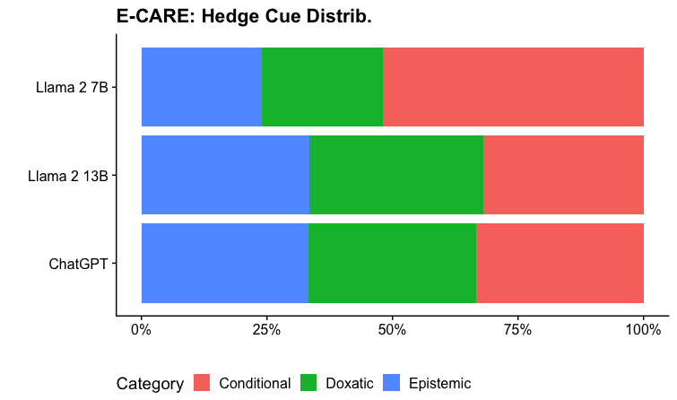<details> <summary>extracted/6246183/hedge-distrib-ecare.png Details</summary>  ### Visual Description ## Horizontal Stacked Bar Chart: E-CARE: Hedge Cue Distrib. ### Overview The image displays a horizontal stacked bar chart titled "E-CARE: Hedge Cue Distrib." It compares the distribution of three categories of "hedge cues" across three different large language models: Llama 2 7B, Llama 2 13B, and ChatGPT. The chart visualizes the proportional composition of each model's output in terms of these categories. ### Components/Axes * **Chart Title:** "E-CARE: Hedge Cue Distrib." (located at the top center). * **Y-Axis (Vertical):** Lists the three models being compared. From top to bottom: "Llama 2 7B", "Llama 2 13B", "ChatGPT". * **X-Axis (Horizontal):** Represents a percentage scale from 0% to 100%. Major tick marks and labels are present at 0%, 25%, 50%, 75%, and 100%. * **Legend:** Located at the bottom of the chart. It defines the color coding for the three categories: * **Red Square:** "Conditional" * **Green Square:** "Doxatic" * **Blue Square:** "Epistemic" * **Data Bars:** Three horizontal bars, one for each model. Each bar is segmented into three colored sections (blue, green, red) whose lengths represent the percentage share of each category. ### Detailed Analysis The chart presents the following approximate percentage distributions for each model. Values are estimated based on the alignment of segment boundaries with the x-axis scale. **1. Llama 2 7B (Top Bar):** * **Epistemic (Blue, left segment):** Extends from 0% to approximately **25%**. * **Doxatic (Green, middle segment):** Extends from ~25% to approximately **50%**. This segment represents about **25%** of the total. * **Conditional (Red, right segment):** Extends from ~50% to 100%. This segment represents about **50%** of the total. * **Trend:** The bar shows a clear majority of "Conditional" cues, with "Epistemic" and "Doxatic" cues making up roughly equal, smaller portions. **2. Llama 2 13B (Middle Bar):** * **Epistemic (Blue, left segment):** Extends from 0% to approximately **30%**. * **Doxatic (Green, middle segment):** Extends from ~30% to approximately **65%**. This segment represents about **35%** of the total. * **Conditional (Red, right segment):** Extends from ~65% to 100%. This segment represents about **35%** of the total. * **Trend:** The distribution is more balanced than Llama 2 7B. "Doxatic" and "Conditional" cues are roughly equal in proportion, with "Epistemic" cues being the smallest category. **3. ChatGPT (Bottom Bar):** * **Epistemic (Blue, left segment):** Extends from 0% to approximately **30%**. * **Doxatic (Green, middle segment):** Extends from ~30% to approximately **65%**. This segment represents about **35%** of the total. * **Conditional (Red, right segment):** Extends from ~65% to 100%. This segment represents about **35%** of the total. * **Trend:** The distribution for ChatGPT appears visually identical to that of Llama 2 13B. ### Key Observations 1. **Model Similarity:** Llama 2 13B and ChatGPT exhibit nearly identical distributions of hedge cue categories, suggesting similar behavior in this specific metric. 2. **Model Difference:** Llama 2 7B shows a distinctly different pattern, with a much higher proportion of "Conditional" cues (~50%) compared to the other two models (~35% each). 3. **Category Dominance:** For Llama 2 7B, "Conditional" is the dominant category. For Llama 2 13B and ChatGPT, no single category is overwhelmingly dominant, with "Doxatic" and "Conditional" being co-dominant. 4. **Epistemic Consistency:** The "Epistemic" category is the smallest segment for all three models, ranging from ~25% to ~30%. ### Interpretation This chart from the E-CARE framework analyzes how different AI models use "hedge cues"—linguistic devices that express uncertainty or caution (e.g., "possibly," "it seems," "I think"). * **What the data suggests:** The distribution indicates a potential scaling effect or architectural difference between Llama 2 7B and its larger 13B counterpart. The 7B model relies more heavily on **Conditional** hedging (e.g., "If X, then Y"), which frames statements within specific conditions. The larger 13B model and ChatGPT shift towards a more balanced use of **Doxatic** hedging (related to belief or opinion, e.g., "I believe," "It is thought") alongside conditional statements. * **Relationship between elements:** The near-identical profiles of Llama 2 13B and ChatGPT are striking. It could imply that at a certain scale or with sufficient training, models converge on a similar strategy for distributing uncertainty across these three linguistic categories. The outlier, Llama 2 7B, may represent a less nuanced or differently optimized approach to hedging. * **Notable implication:** The type of hedging a model uses can affect the perceived reliability, tone, and safety of its outputs. A model heavy in conditional cues might sound more logically precise but also more restrictive, while one using more doxatic cues might sound more opinionated or subjective. This analysis provides a quantitative lens into the qualitative "voice" of different AI systems. </details> Figure 18: Distribution of hedge cues across incorrect explanations. #### A.10.3 E-CARE Concept Drift See Figure 13. #### A.10.4 E-CARE Coherence See Figure 15. #### A.10.5 E-CARE Uncertainty See Figure 16. #### A.10.6 E-CARE Hedge Ratio See Figure 17. #### A.10.7 E-CARE Hedge Distribution See Figure 18. 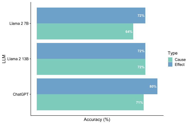### A.11 Causal Directionality <details> <summary>extracted/6246183/cause-effect-acc.png Details</summary>  ### Visual Description ## Horizontal Grouped Bar Chart: LLM Accuracy on Cause vs. Effect Tasks ### Overview The image displays a horizontal grouped bar chart comparing the performance of three Large Language Models (LLMs) on two distinct task types: "Cause" and "Effect." The chart measures performance in terms of accuracy percentage. ### Components/Axes * **Chart Type:** Horizontal Grouped Bar Chart. * **Y-Axis (Vertical):** Labeled "LLM". It lists three models from top to bottom: 1. Llama 2 7B 2. Llama 2 13B 3. ChatGPT * **X-Axis (Horizontal):** Labeled "Accuracy (%)". The axis has numerical markers at 0, 20, 40, 60, 80, and 100. * **Legend:** Positioned on the right side of the chart, titled "Type". It defines the color coding: * **Cause:** Represented by a teal/green color. * **Effect:** Represented by a blue color. * **Data Labels:** Each bar has its exact accuracy percentage printed at its end. ### Detailed Analysis The chart presents paired bars for each LLM, showing accuracy for "Cause" and "Effect" tasks. **1. Llama 2 7B (Top Group)** * **Effect (Blue Bar):** The bar extends to the 72% mark. **Trend:** This is the higher-performing task for this model. * **Cause (Teal Bar):** The bar extends to the 64% mark. **Trend:** This is the lower-performing task for this model. * **Comparison:** The model shows an 8 percentage point higher accuracy on "Effect" tasks compared to "Cause" tasks. **2. Llama 2 13B (Middle Group)** * **Effect (Blue Bar):** The bar extends to the 72% mark. * **Cause (Teal Bar):** The bar extends to the 72% mark. * **Comparison:** The model demonstrates perfectly balanced performance, with identical accuracy on both task types. **3. ChatGPT (Bottom Group)** * **Effect (Blue Bar):** The bar extends to the 80% mark. **Trend:** This is the highest accuracy value shown on the entire chart. * **Cause (Teal Bar):** The bar extends to the 71% mark. * **Comparison:** The model shows a 9 percentage point higher accuracy on "Effect" tasks compared to "Cause" tasks. ### Key Observations 1. **Performance Hierarchy:** ChatGPT achieves the highest single accuracy score (80% on Effect). Llama 2 7B has the lowest single score (64% on Cause). 2. **Task Difficulty Pattern:** For two of the three models (Llama 2 7B and ChatGPT), the "Effect" task yields higher accuracy than the "Cause" task. Llama 2 13B is the exception with equal performance. 3. **Model Scaling (Llama 2):** Increasing the model size from 7B to 13B parameters significantly improved accuracy on the "Cause" task (from 64% to 72%, an 8-point gain) while maintaining the same accuracy on the "Effect" task (72%). 4. **Overall Range:** Accuracy scores across all models and tasks range from 64% to 80%, a spread of 16 percentage points. ### Interpretation This chart provides a comparative snapshot of LLM capabilities in causal reasoning, segmented into understanding causes versus predicting effects. * **What the data suggests:** The data indicates that, for the evaluated models and tasks, predicting or understanding *effects* may be a slightly easier or better-learned capability than identifying *causes*. This could reflect biases in training data (more effect descriptions) or an inherent complexity difference in the tasks as framed. * **How elements relate:** The direct side-by-side comparison for each model isolates the task-type variable, allowing for a clear assessment of each model's strengths and weaknesses within causal reasoning. The scaling comparison within the Llama 2 family shows that increased model capacity primarily benefits the more challenging task ("Cause" for the 7B model). * **Notable patterns/anomalies:** The perfect balance (72%/72%) of Llama 2 13B is a notable pattern, suggesting a different internal representation or training outcome compared to its smaller sibling and ChatGPT. The consistent outperformance of "Effect" tasks by the other two models is the dominant trend. The chart does not provide context on the specific datasets or evaluation methodologies used, which is critical for a full interpretation of these accuracy figures. </details> Figure 19: Accuracy in predicting the most plausible causes vs effects on COPA. When considering the causal directionality (i.e. cause vs effect), we observed that accuracy tended to differ between LLMs on COPA. In particular, we found both GPT and LLaMA 2 7B to be more accurate in predicting the effects in causal scenarios (see Figure 19). We hypothesize that LLMs may suffer the challenge of causal sufficiency as the space of potential causal explanations can be far greater than the range of effects once an event has been observed. This hypothesis is partly supported by the fact that GPT and LLaMA 2 7B express greater linguistic uncertainty and produce more complex explanations when predicting causes rather than effects. ### A.12 Dataset Details COPA is released under a BSD-2 license and made available for broad research usage with copyright notification restrictions people.ict.usc.edu/~gordon/copa.html. We do not modify or use COPA outside of its intended use which is primarily open-domain commonsense causal reasoning. E-CARE is released under the MIT license and can be used for broad purposes with copyright notification restrictions github.com/Waste-Wood/e-CARE?tab=MIT-1-ov-file#readme. We do not modify or use E-CARE outside of its intended use which is causal reasoning evaluation of language models.