## Recursive Speculative Decoding: Accelerating LLM Inference via Sampling Without Replacement
Wonseok Jeon 1 Mukul Gagrani 1 Raghavv Goel 1 Junyoung Park 1 Mingu Lee * 1 Christopher Lott * 1
## Abstract
Speculative decoding is an inference-acceleration method for large language models (LLMs) where a small language model generates a draft-token sequence which is further verified by the target LLMinparallel. Recent works have advanced this method by establishing a draft-token tree, achieving superior performance over a single-sequence speculative decoding. However, those works independently generate tokens at each level of the tree, not leveraging the tree's entire diversifiability. Besides, their empirical superiority has been shown for fixed length of sequences, implicitly granting more computational resource to LLM for the tree-based methods. None of the existing works has conducted empirical studies with fixed target computational budgets despite its importance to resource-bounded devices. We present Recursive Speculative Decoding (RSD), a novel tree-based method that samples draft tokens without replacement and maximizes the diversity of the tree. During RSD's drafting, the tree is built by either Gumbel-Topk trick that draws tokens without replacement in parallel or Stochastic Beam Search that samples sequences without replacement while early-truncating unlikely draft sequences and reducing the computational cost of LLM. We empirically evaluate RSD with Llama 2 and OPT models, showing that RSD outperforms the baseline methods, consistently for fixed draft sequence length and in most cases for fixed computational budgets at LLM.
* Equal advising 1 Qualcomm AI Research. Correspondence to: Wonseok Jeon < wjeon@qti.qualcomm.com > , Mingu Lee < mingul@qti.qualcomm.com > , Christopher Lott < clott@qti.qualcomm.com > .
Qualcomm AI Research is an initiative of Qualcomm Technologies, Inc.
## 1. Introduction
Large language models (LLMs) (Touvron et al., 2023; Zhang et al., 2022; Brown et al., 2020; Achiam et al., 2023; Jiang et al., 2023) have gained popularity due to their outstanding achievements with high-quality text generation, which has drastically increased demands for faster text generation. However, auto-regressive nature of LLMs limits text generation to produce a single token at a time and often suffers from memory-bandwidth bottleneck, which leads to slower inference (Shazeer, 2019). translation (Xiao et al., 2023).
Speculative decoding (Chen et al., 2023; Leviathan et al., 2023) has emerged as a solution for LLM inference acceleration by leveraging the innate parallelizability of the transformer network (Vaswani et al., 2017). This decoding method utilizes a draft model, i.e., a smaller language model, to auto-regressively generate a sequence of draft tokens with a significantly lower cost and latency, followed by the target LLM producing the token-wise probability distributions in parallel. Rejection sampling then verifies those draft tokens, recovering the sequence distribution by auto-regressive decoding with the target model. As speculative decoding uses a single sequence of draft tokens, one needs to increase the draft-sequence length to better exploit LLM's parallelizability. However, the longer draft sequence may slow down the overall inference in practice due to the computational overhead caused by additional auto-regressive decoding steps from the draft model, possibly decelerating the target model process due to the increased number of draft tokens.
Recent works on tree-based speculative decoding (Sun et al., 2023; Miao et al., 2023) have achieved better diversity and higher acceptance rate via multiple draft-token sequences. Despite promising results, their decoding methods independently sample the draft tokens, often harming the diversity of the tree when samples overlap. Also, their experiments have been conducted for the fixed length of draft-token sequences across decoding methods, implicitly requiring more computational resource to the target model when using tree-based methods. To the best of our knowledge, no prior work has thoroughly investigated the performance of single-sequence and tree-based speculative decoding methods with fixed target computational budget, which has practical importance
for resource-bounded devices.
We propose R ecursive S peculative D ecoding (RSD), a novel tree-based speculative decoding algorithm that fully exploits the diversity of the draft-token tree by using sampling without replacement. We summarize our contributions as below:
Theoretical contribution. We propose recursive rejection sampling capable of recovering the target model's distribution with the sampling-without-replacement distribution defined by the draft model.
Algorithmic contribution. We present RSD which builds draft-token tree composed of the tokens sampled without replacement . Two tree construction methods, RSD with C onstant branching factors (RSD-C) and RSD with S tochastic Beam Search (RSD-S) (Kool et al., 2019), are proposed.
Empirical contribution. Two perspectives are considered in our experiments: ( Exp1 ) performance for fixed length of draft sequence , which is also widely considered in previous works (Sun et al., 2023; Miao et al., 2023), and ( Exp2 ) performance for fixed target computational budget , where we compared methods with given size of the draft-token tree. RSD is shown to outperform the baselines consistently in ( Exp1 ) and for the majority of experiments in ( Exp2 ) .
## 2. Background
Let us consider a sequence generation problem with a set X of tokens. We also assume that there is a target model characterized by its conditional probability q ( x i +1 | x 1: i ) := Pr { X i +1 = x i +1 | X 1: i = x 1: i } , i ∈ N for x 1: i := ( x 1 , ..., x i ) , where X 1 , ..., X i +1 ∈ X and x 1 , ..., x i +1 ∈ X are random tokens and their realizations, respectively. Given an input sequence X 1: t = x 1: t , we can auto-regressively and randomly sample an output sequence X t +1: t + i for i ∈ N , i.e., X t + i +1 ∼ q ( ·| X 1: t + i ) .
Speculative decoding. Auto-regressive sampling with modern neural network accelerators (e.g., GPU/TPU) is known to suffer from the memory-bandwidth bottleneck (Shazeer, 2019), which prevents us from utilizing the entire computing power of those accelerators. Speculative decoding (Leviathan et al., 2023; Chen et al., 2023) addresses such issue by using the target model's parallelizability. It introduces a (small) draft model which outputs p ( ˆ X i +1 | ˆ X 1: i ) := Pr { ˆ X i +1 = ˆ x i +1 | ˆ X 1: i = ˆ x 1: i } , i ∈ N . Speculative decoding accelerates the inference speed by iteratively conducting the following steps:
1) Draft token generation: For an input sequence X 1: m = x 1: m and the draft sequence length L , sample draft tokens ˆ X n +1 ∼ p ( ·| X 1: m , ˆ X m +1: n ) auto-regressively for n = m,..., m + L -1 (where ˆ X m +1: m = ∅ ).
2) Evaluation with target model: Use the target model to compute q ( ·| X 1: m , ˆ X m +1: n ) , n = m,..., m + L in parallel.
3) Verification via rejection sampling: Starting from n = m + 1 to m + L , sequentially accept the draft token ˆ X n (i.e., X n = ˆ X n ) with the probability min { 1 , q ( ˆ X n | X 1: n -1 ) p ( ˆ X n | X 1: n -1 ) } . If one of the draft tokens ˆ X n is rejected, we sample X n ∼ q res ( ·| X 1: n -1 ) , where the residual distribution is defined by
$$q _ { r e s } ( \cdot | \tau ) \colon = N o r m [ [ q ( \cdot | \tau ) - p ( \cdot | \tau ) ] ^ { + } ] ,$$
for [ f ] + := max { 0 , f ( · ) } and Norm[ f ] := f ∑ x ′ ∈X f ( x ′ ) . If all draft tokens are accepted ( X n = ˆ X n for n = m + 1 , ..., m + L ), sample an extra token X m + L +1 ∼ q ( ·| X 1: m + L ) .
Chen et al. (2023) and Leviathan et al. (2023) have shown that the target distribution can be recovered when rejection sampling is applied.
Tree-based speculative decoding. One can further improve the sequence generation speed by using multiple draft-token sequences, or equivalently, a tree of draft tokens.
SpecTr (Sun et al., 2023) is a tree-based speculative decoding algorithm motivated by the Optimal Transport (OT) (Villani et al., 2009). It generalizes speculative decoding with K i.i.d. draft tokens ˆ X ( k ) ∼ p, k = 1 , ..., K, while recovering the target distribution q . To this end, a K -sequential draft selection algorithm ( K -SEQ) was proposed, where the algorithm decides whether to accept K draft tokens ˆ X ( k ) , k = 1 , ..., K, or not with the probability min { 1 , q ( ˆ X ( k ) ) γ · p ( ˆ X ( k ) ) } , γ ∈ [1 , K ] . If all draft tokens are rejected, we use a token drawn from the residual distribution
$$\begin{array} { r l } & { \in \mathcal { X } } \\ & { \quad N o r m \left [ q - \min \left \{ p , \frac { q } { \gamma } \right \} \frac { 1 - ( 1 - \beta _ { p , q } ( \gamma ) ) ^ { K } } { \beta _ { p , q } ( \gamma ) } \right ] } \\ & { y a n d \in \mathbb { N } , \quad f o r \, \beta _ { p , q } ( \gamma ) \colon = \sum _ { x \in \mathcal { X } } \min \{ p ( x ) , q ( x ) / \gamma \} . } \end{array}$$
SpecInfer also used the draft-token tree to speed up the inference with multiple draft models p ( k ) , k = 1 , ..., K (Miao et al., 2023). During the inference of SpecInfer, all draft models generate their own draft tokwns independently and create a draft-token tree collectively through repetetion. For draft verification, multi-round rejection sampling is used to recover the target distribution, where we determine whether to accept one of the draft tokens or not with probability min { 1 , q ( k ) ( ˆ X ( k ) ) p ( k ) ( ˆ X ( k ) ) } with distributions q (1) := q and q ( k ) := Norm [ [ q ( k -1) -p ( k -1) ] + ] , k = 2 , ..., K + 1 . If all draft tokens are rejected, we sample a token Y ∼ q ( K +1) from the last residual distribution.
## 3. Recursive Speculative Decoding
In this section, we present R ecursive S peculative D ecoding (RSD), a tree-based speculative decoding method that constructs draft-token trees via sampling without replacement.
## Algorithm 1 Recursive Rejection Sampling
- 1: Input: Draft dist. p ( k ) , k = 1 , ..., K, target dist. q .
- 2: Sample ˆ X ( k ) by (1).
- 3: Compute q ( k ) ( ·| ˆ X (1: k -2) ) and Θ ( k ) by (2) and (3).
- 4: for k in { 1 , ..., K } do
- 5: Sample A ( k ) ∈ { acc , rej } with probability Θ ( k ) .
- 6: if A ( k ) = acc then return Z ← ˆ X ( k ) ; end if
- 7: end for
- 8: return Z ∼ q ( K +1) ( ·| ˆ X (1: K -1) )
We first propose recursive rejection sampling, a generalization of multi-round speculative decoding (Miao et al., 2023) that is applicable to draft distributions with dependencies, where sampling-without-replacement distribution is one instance of such distributions. Then, we use recursive rejection sampling to validate each level of the draft-token tree which can be efficiently constructed via either Gumbel-Topk trick (Vieira, 2014) and Stochastic Beam Search (Kool et al., 2019),
## 3.1. Recursive Rejection Sampling: Generalized Multi-Round Rejection Sampling
Suppose we have target distribution q ( x ) , x ∈ X . In recursive rejection sampling, we introduce random variables ˆ X (1) , ..., ˆ X ( K ) ∈ X that represent K draft tokens; these tokens will locate at the same level of the draft-token tree in Section 3.2. We aim to recover target distribution q , where
<!-- formula-not-decoded -->
for some distributions p ( k ) , k = 1 , ..., K and a sequence ˆ X (1: k -1) := ( ˆ X (1) , ..., ˆ X ( k -1) ) . Note that we assume distributions with dependencies unlike prior works such as SpecTr (Sun et al., 2023) consider independent distributions. By using p (1) , ..., p ( K ) and q , we define q (1) := q and residual distributions
$$& q ^ { ( k + 1 ) } ( \cdot | x ^ { ( 1 \colon k - 1 ) } ) \\ & \quad \vdots = N o r m \left [ [ q ^ { ( k ) } ( \cdot | x ^ { ( 1 \colon k - 2 ) } ) - p ^ { ( k ) } ( \cdot | x ^ { ( 1 \colon k - 1 ) } ) ] + \right ] \quad ( 2 )$$
for k = 1 , ..., K and x (1) , ..., x ( K +1) ∈ X , where x (1: k ′ ) = ∅ (empty sequence, i.e., no conditioning) if k ′ < 1 , or ( x (1) , ..., x ( k ′ ) ) , otherwise. Together with draft, target, and residual distributions, recursive rejection sampling introduces threshold random variables Θ (1) , ..., Θ ( K ) ∈ [0 , 1] which determines rejection criteria for each draft token ˆ X ( k ) , k = 1 , ..., K :
$$\Theta ^ { ( k ) } \colon = \min \left \{ 1 , \frac { q ^ { ( k ) } ( \hat { X } ^ { ( k ) } | \hat { X } ^ { ( 1 \colon k - 2 ) } ) } { p ^ { ( k ) } ( \hat { X } ^ { ( k ) } | \hat { X } ^ { ( 1 \colon k - 1 ) } ) } \right \} . \quad ( 3 )$$
Specifically, each Θ ( k ) can be used to define random variables A ( k ) ∈ { acc , rej } (where acc and rej indicate ac-
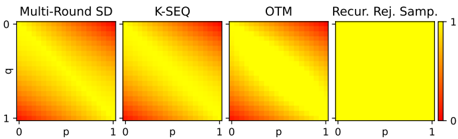
Figure 1. Acceptance rates for multi-round speculative decoding, K-SEQ, OTM and recursive rejection sampling are given when Ber( p ) and Ber( q ) are draft and target distributions, respectively, and two tokens are proposed by the draft model ( K = 2 ).
<details>
<summary>Image 1 Details</summary>
### Visual Description
\n
## Heatmaps: Performance Comparison of Sampling Methods
### Overview
The image presents four heatmaps, each representing the performance of a different sampling method: Multi-Round SD, K-SEQ, OTM, and Recur. Rej. Samp. The heatmaps visualize the relationship between two parameters, 'p' and 'q', with performance indicated by color intensity. The color scale ranges from 0 (blue/dark) to 1 (red/light), suggesting higher values represent better performance.
### Components/Axes
Each heatmap shares the same axes:
* **X-axis:** Labeled 'p', ranging from 0 to 1.
* **Y-axis:** Labeled 'q', ranging from 0 to 1.
* **Color Scale:** A gradient from blue (approximately 0) to red (approximately 1), positioned to the right of the four heatmaps.
The four heatmaps are arranged horizontally, each with a title indicating the sampling method:
1. Multi-Round SD
2. K-SEQ
3. OTM
4. Recur. Rej. Samp.
### Detailed Analysis or Content Details
**1. Multi-Round SD:**
* The heatmap shows a generally upward trend. Values are low (close to 0, yellow) in the bottom-left corner (low p, low q) and increase towards high values (close to 1, red) in the top-right corner (high p, high q).
* The gradient is relatively smooth.
**2. K-SEQ:**
* Similar to Multi-Round SD, this heatmap also exhibits an upward trend. Values are low in the bottom-left and increase towards the top-right.
* The gradient appears slightly steeper than Multi-Round SD.
**3. OTM:**
* This heatmap also shows an upward trend, but the gradient is less pronounced than the previous two.
* The color transition is more gradual, with a larger area of intermediate values.
**4. Recur. Rej. Samp.:**
* This heatmap displays a downward trend. Values are high (close to 1, red) in the bottom-left corner (low p, low q) and decrease towards low values (close to 0, yellow) in the top-right corner (high p, high q).
* The gradient is relatively smooth.
### Key Observations
* Three of the methods (Multi-Round SD, K-SEQ, and OTM) show a positive correlation between 'p' and 'q' and performance. Increasing both parameters leads to better results.
* Recur. Rej. Samp. exhibits an inverse correlation – increasing both 'p' and 'q' leads to *worse* results.
* K-SEQ appears to have the steepest gradient, suggesting it is most sensitive to changes in 'p' and 'q'.
* OTM appears to be the least sensitive to changes in 'p' and 'q'.
### Interpretation
The heatmaps compare the performance of four different sampling methods across a range of parameter values 'p' and 'q'. The differing trends suggest that each method responds differently to these parameters. The positive correlation observed in Multi-Round SD, K-SEQ, and OTM indicates that increasing both 'p' and 'q' generally improves performance for these methods. Conversely, the negative correlation in Recur. Rej. Samp. suggests that this method performs best when 'p' and 'q' are low.
The differences in gradient steepness suggest varying sensitivities to parameter changes. K-SEQ's steeper gradient implies that small adjustments to 'p' and 'q' can significantly impact its performance, while OTM is more robust to such changes.
This data could be used to select the most appropriate sampling method for a given application, based on the desired values of 'p' and 'q' and the level of sensitivity required. The specific meaning of 'p' and 'q' is not provided in the image, but they likely represent parameters controlling the sampling process itself.
</details>
ceptance and rejection of draft tokens, respectively) such that Pr { A ( k ) = acc | Θ ( k ) = θ } = θ for θ ∈ [0 , 1] .
Finally, recursive rejection sampling can be characterized by defining a random variable Z ∈ X such that
<!-- formula-not-decoded -->
where A (1: k -1) := ( A (1) , ..., A ( k -1) ) and rej k is a lengthk sequence with all of its elements equal to rej . Intuitively, we select ˆ X (1) if it is accepted ( A (1) = acc ); we select ˆ X ( k ) when all previous draft tokens ˆ X (1) , ..., ˆ X ( k -1) are rejected and ˆ X ( k ) is accepted ( A (1: k -1) = rej k -1 , A ( k ) = acc ) for each k ; we sample Y ∼ q ( K +1) ( ·| ˆ X (1: K -1) ) and select Y if all draft tokens are rejected ( A (1: K ) = rej K ). We summarize the entire process of recursive rejection sampling in Algorithm 1 . Note that the original rejection sampling (Leviathan et al., 2023; Chen et al., 2023) is a special case of our recursive rejection sampling with K = 1 . Also, it can be shown that recursive rejection sampling (4) always recovers the target distribution q :
Theorem 3.1 (Recursive rejection sampling recovers target distribution) . For the random variable Z ∈ X in (4) ,
$$\Pr \{ Z = z \} = q ( z ) , z \in \mathcal { X } .$$
$$P r o f . \, S e e \, A p p e n d i x \, A . 1 .$$
Although the proposed recursive rejection sampling is applicable to arbitrary distributions with dependencies following (1), we assume a single draft model (as in SpecTr (Sun et al., 2023) and focus on the cases where the draft model samples predictive tokens without replacement, which is an instance of (1).
Toy example. We present a didactic example with Bernoulli distributions (given by Sun et al. (2023)) to showcase the benefit of recursive rejection sampling. Suppose that Bernoulli distributions are used for both draft and target models and only K = 2 tokens are allowed for draft proposals. The acceptance rates for different methods are depicted
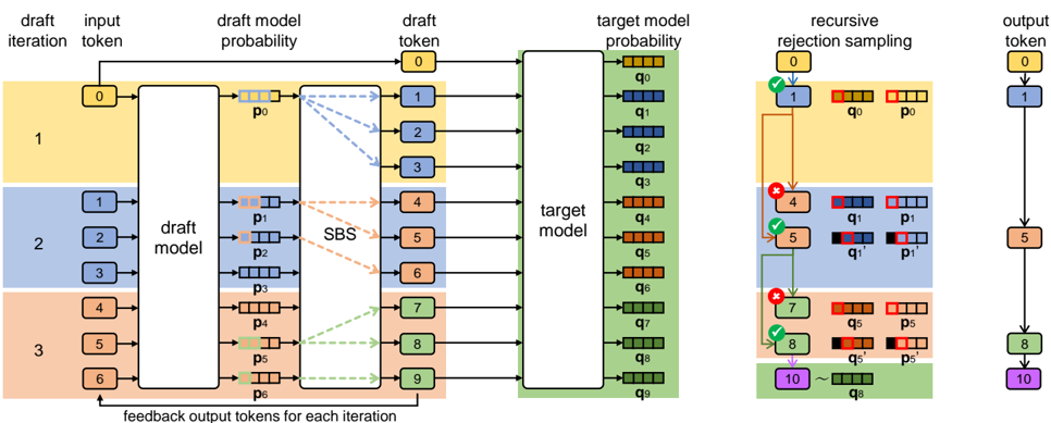
Figure 2. We describe the entire process of RSD with Stochastic Beam Search (RSD-S); the difference between RSD-S and RSD with Constant branching factors (RSD-C) lies at the method of constructing the draft-token tree. Draft tokens the tree are sampled in parallel at each level and auto-regressively across levels, while Stochastic Beam Search samples sequences without replacement at each tree level. The established draft-token tree is then processed by the target model in parallel, which lets us acquire the token-wise target model probabilities. Finally, recursive rejection sampling (for sampling-without-replacement distribution) is applied to each level of the tree, recovering the sequence generation distribution of the target model.
<details>
<summary>Image 2 Details</summary>
### Visual Description
\n
## Diagram: Recursive Rejection
</details>
in Figure 1; multi-round speculative decoding (from SpecInfer (Miao et al., 2023)), K-SEQ and Optimal Transport with Membership costs (OTM) (Sun et al., 2023), use sampling with replacement, whereas recursive rejection sampling uses sampling without replacement; note that both K-SEQ and OTM were presented in SpecTr paper (Sun et al., 2023) where OTM shows theoretically optimal acceptance rate. For all the baselines, acceptance rates decrease as the discrepancy between draft and target distribution increases, since tokens sampled from draft models become more unlikely from target models. On the other hand, recursive rejection sampling achieves 100% acceptance rate even with high draft-target-model discrepancy; once the first draft token is rejected, the second draft token is always aligned with the residual distribution. This example shows that draft distributions with dependencies, e.g., sampling-withoutreplacement distribution, leads to higher acceptance rate and becomes crucial, especially for the cases with higher distributional discrepancy between draft and target.
## 3.2. Tree-Based Speculative Decoding with Recursive Rejection Sampling
Recursive rejection sampling is applicable to tree-based speculative decoding algorithms if sampling without replacement is used to construct a draft-token tree . Two Recursive Speculative Decoding (RSD) algorithms using recursive rejection sampling are presented in this section, while they share the same pipeline for parallel target evaluation and draft tree verification after building the draft-token tree (See
Figure 2. ). We describe details about how RSD works in the following sections.
## 3.2.1. DRAFT-TOKEN TREE GENERATION
We consider two RSD algorithms: RSD with C onstant branching factors (RSD-C) and RSD with S tochastic Beam Search (RSD-S). RSD-C builds the draft-token tree having constant branching factors, which makes sequences from the tree to have the same length. RSD-S, on the other hand, builds the tree via Stochastic Beam Search (Kool et al., 2019) that samples draft sequences without replacement, while truncating sequences that are unlikely to be generated from the draft model and efficiently handling the computational cost.
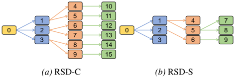
RSD with Constant branching factors (RSD-C). Let L denote the fixed length for all draft sequences, which is equivalent to the depth of the draft-token tree, and τ (1) 0 denote the input sequence of tokens. Let us assume that the tree level increases from root ( l = 0 ) to leaf ( l = L ) nodes, where each node is characterized by the (partial) sequence. We also define b := ( b 0 , ..., b L -1 ) where b l is the branching factor at the level l (See Figure 3(a) for the example with b = (3 , 2 , 1) .).
At each level l ∈ { 0 , ..., L -1 } of the draft tree, we begin with N l sequences τ ( k ) l , k = 1 , ..., N l generated from the previous level, where N 0 := 1 and N l := ∏ l -1 l ′ =0 b l ′ for l ≥ 1 . Then, we evaluate log probabilities ϕ l ( τ ( k ) l , · ) and perturbed log probabilities ˜ ϕ l ( τ ( k ) l , · ) for each k , i.e., for
Figure 3. We describe examples of constructing draft-token trees with the (maximum) draft length equal to 3; (a) The tree constructed by RSD-C with branching factors b = (3 , 2 , 1) is given; (b) we depict the tree constructed by RSD-S with beamwidth W = 3 , where edges are determined via Stochastic Beam Search.
<details>
<summary>Image 3 Details</summary>
### Visual Description
\n
## Diagram: RSD-C and RSD-S Flow Diagrams
### Overview
The image presents two flow diagrams, labeled (a) RSD-C and (b) RSD-S. Both diagrams depict a process where an initial node (0) branches out to multiple subsequent nodes. The diagrams illustrate different connection patterns between the initial node and the final nodes.
### Components/Axes
The diagrams consist of rectangular nodes numbered 0 through 15. Arrows indicate the flow or connection between nodes. The diagrams are labeled as follows:
* **(a) RSD-C**: Represents a complex branching structure.
* **(b) RSD-S**: Represents a simpler, more sequential structure.
### Detailed Analysis or Content Details
**Diagram (a) RSD-C:**
* Node 0 (yellow) branches out to nodes 1, 2, and 3 (blue).
* Nodes 1, 2, and 3 each connect to nodes 4, 5, 6, 7, 8, and 9 (orange).
* Nodes 4 through 9 each connect to nodes 10 through 15 (green).
* Specifically:
* Node 1 connects to nodes 10, 11.
* Node 2 connects to nodes 12, 13.
* Node 3 connects to nodes 14, 15.
**Diagram (b) RSD-S:**
* Node 0 (yellow) branches out to nodes 1, 2, and 3 (blue).
* Node 1 connects to node 4 (orange).
* Node 2 connects to node 5 (orange).
* Node 3 connects to node 6 (orange).
* Nodes 4, 5, and 6 each connect to nodes 7, 8, and 9 (green).
* Specifically:
* Node 4 connects to nodes 7, 8, 9.
* Node 5 connects to nodes 7, 8, 9.
* Node 6 connects to nodes 7, 8, 9.
### Key Observations
* RSD-C exhibits a fully connected structure between the intermediate (blue) and final (green) nodes, while RSD-S has a more limited connection.
* RSD-S shows a convergence of connections to the final nodes 7, 8, and 9.
* Both diagrams start with the same initial branching from node 0 to nodes 1, 2, and 3.
### Interpretation
These diagrams likely represent different strategies for distributing or processing information. RSD-C (Complex) suggests a scenario where all possible combinations of intermediate nodes are considered before reaching the final nodes. This could represent a thorough exploration of options or a parallel processing approach. RSD-S (Sequential) suggests a more streamlined process where each intermediate node leads to a specific subset of final nodes. This could represent a more efficient or targeted approach. The diagrams demonstrate two distinct architectural patterns for a system, potentially related to routing, decision-making, or data flow. The numbering of the nodes suggests a sequential or ordered process, but the diagrams themselves do not provide information about the nature of the process or the meaning of the numbers. The diagrams are abstract representations and require additional context to fully understand their purpose.
</details>
i.i.d. Gumbel samples G ( k ) l ( x ) , x ∈ X ,
$$\phi _ { l } ( \tau _ { l } ^ { ( k ) } , \cdot ) \colon = \log p ( \cdot | \tau _ { l } ^ { ( k ) } ) , \quad ( 5 ) \quad \begin{array} { r l r } & { ^ { l } } \\ & { ( b ) \, i d o t a n g e \, . } \end{array}$$
$$\tilde { \phi } _ { l } ( \tau _ { l } ^ { ( k ) } , \cdot ) \colon = \phi _ { l } ( \tau _ { l } ^ { ( k ) } , \cdot ) + G _ { l } ^ { ( k ) } , \quad ( 6 ) \quad t h e$$
where both log probabilities and Gumbel samples can be computed in parallel; proper positional encodings and attention masking (Cai et al., 2023; Miao et al., 2023) are required for the parallel log-probability computation when transformer architecture is used (Vaswani et al., 2017). By using Gumbel-Topk trick (Vieira, 2014; Kool et al., 2019) with perturbed log probabilities (6), one can sample topb l tokens without replacement for each sequence τ ( k ) l :
$$\hat { X } _ { l + 1 } ^ { ( ( k - 1 ) b _ { l } + 1 ) } , \dots , \hat { X } _ { l + 1 } ^ { ( ( k - 1 ) b _ { l } + b _ { l } ) } = \underset { x \in \mathcal { X } } { \arg t o p \text {-} b _ { l } } \left ( \tilde { \phi } _ { l } ( \tau _ { l } ^ { ( k ) } , x ) \right ) . \quad \text {where} \, t h i n d e r s$$
Note that the outputs ˆ X (( k -1) b l + k ′ ) l +1 , k ′ = 1 , ..., b l , in (7) are assumed to be in the decreasing order of values ˜ ϕ l ( τ ( k ) l , ˆ X (( k -1) b l + k ′ ) l +1 ) , for each k . Finally, we define
$$O _ { l + 1 } ^ { ( ( k - 1 ) b _ { l } + k ^ { \prime } ) } \colon = ( \hat { X } _ { l + 1 } ^ { ( ( k - 1 ) b _ { l } + k ^ { \prime } ) } , k ) , \quad ( 8 ) \quad \psi$$
$$\tau _ { l + 1 } ^ { ( ( k - 1 ) b _ { l } + 1 ) } \colon = ( \tau _ { l } ^ { ( k ) } , \hat { X } _ { l + 1 } ^ { ( ( k - 1 ) b _ { l } + 1 ) } ) \quad ( 9 )$$
for k ∈ 1 , ..., N l and k ′ ∈ { 1 , ..., b l } , where O (( k -1) b l + k ′ ) l +1 is a pair of draft token and parent sequence index. Those pairs in (8) are stored for all levels l = 0 , ..., L -1 and used for draft tree verification, which exploits the fact that the tokens ˆ X (( k -1) b l +1) l +1 , ..., ˆ X (( k -1) b l + b l ) l +1 follow sampling without replacement from p ( ·| τ ( k ) l ) for any given parent sequence index k .
RSD with Stochastic Beam Search (RSD-S). One caveat of RSD-C is that its constant branching factors b should be carefully determined to handle tree complexity, when the computation budget is limited; for example, if b = ( n, ..., n ) with its length L , the number of nodes in the draft tree will be ∑ L -1 l =0 n l = O ( n L -1 ) , which is computationally prohibitive for large n and L . Also, RSD-C constructs sequences at each level l by using the myopic token-wise log probabilities ϕ l in (6). RSD-S addresses both issues by using Stochastic Beam Search (Kool et al., 2019) that early-truncates unlikely sequences and utilizes far-sighted sequence log probabilities.
Let us define the maximum draft sequence length L and the beamwidth W . We also define τ (1) 0 as the input sequence similar to RSD-C. At each level l ∈ { 0 , ..., L -1 } , SBS uses beam
$$\mathcal { B } _ { l } & \colon = ( t _ { l } ^ { ( 1 ) } , \dots , t _ { l } ^ { ( W ) } ) , \\ t _ { l } ^ { ( k ) } & \colon = ( \tau _ { l } ^ { ( k ) } , \phi _ { l - 1 } ( \tau _ { l } ^ { ( k ) } ) , \psi _ { l - 1 } ( \tau _ { l } ^ { ( k ) } ) )$$
generated from the previous level l -1 1 . Here, each tuple t ( k ) l for k ∈ { 1 , ..., W } consists of (a) a sequence τ ( k ) l , (b) its sequence log probability ϕ l -1 ( τ ( k ) l ) of τ ( k ) l , and (c) the transformed (perturbed and truncated) sequence log probability ψ l -1 ( τ ( k ) l ) , respectively.
For each tuple t ( k ) l in the beam B l , we evaluate the (nextlevel) sequence log probabilities ϕ l ( τ ( k ) l , · ) and the perturbed sequence log probabilities ˜ ϕ l ( τ ( k ) l , · ) . Specifically for i.i.d. Gumbel samples G ( k ) l ( x ) , x ∈ X , we compute
$$\begin{array} { r l } & { \phi _ { l } ( \tau _ { l } ^ { ( k ) } , \cdot ) \colon = \phi _ { l - 1 } ( \tau _ { l } ^ { ( k ) } ) + \log p ( \cdot | \tau _ { l } ^ { ( k ) } ) , } \\ & { \tilde { \phi } _ { l } ( \tau _ { l } ^ { ( k ) } , \cdot ) \colon = \phi _ { l } ( \tau _ { l } ^ { ( k ) } , \cdot ) + G _ { l } ^ { ( k ) } , } \end{array}$$
where the terms τ ( k ) l and ϕ l -1 ( τ ( k ) l ) within the tuple t ( k ) l of within the beam B l are reused. Similar to RSD-C, both log probabilities and Gumbel samples can be parallelly computed with positional encodings and attention masking (Cai et al., 2023; Miao et al., 2023). In addition to the perturbed log probabilities, SBS in RSD-S transforms ˜ ϕ l ( τ ( k ) l , · ) into the truncated function
$$\begin{array} { r l r } { 8 ) } & \psi _ { l } ( \tau _ { l } ^ { ( k ) } , \cdot ) \colon = T ( \psi _ { l - 1 } ( \tau _ { l } ^ { ( k ) } ) , \tilde { \phi } _ { l } ( \tau _ { l } ^ { ( k ) } , \cdot ) ) , } & { ( 1 0 ) } \end{array}$$
$$T ( u , \phi ) \colon = - \log \left ( e ^ { - u } - e ^ { - \max \phi } + e ^ { - \phi ( \cdot ) } \right ) \quad ( 1 1 )$$
for max ϕ := max x ∈X ϕ ( x ) by reusing ψ l -1 ( τ ( k ) l ) in t ( k ) l . Note that T ( u, ϕ ) in (11) is monotonically increasing w.r.t. ϕ and transforms ϕ to the function with the upper bound u (Kool et al., 2019) 2
After evaluating ψ l ( τ ( k ) l , · ) for all parent sequences τ ( k ) l s, SBS selects topW pairs ( ˆ X l +1 , p l +1 ) of draft token and parent sequence index across the beam B l , i.e.,
$$\begin{array} { r l } { \quad O _ { l + 1 } ^ { ( 1 ) } , \cdots , O _ { l + 1 } ^ { ( W ) } \colon = \underset { ( x , k ) \in \mathcal { X } \times \mathcal { K } } { \arg t o p - W } \left ( \psi _ { l } ( \tau _ { l } ^ { ( k ) } , x ) \right ) \quad ( 1 2 ) } \end{array}$$
$$\frac { ^ { 1 } \text {For} \, l = 0 , \phi _ { - 1 } ( \tau _ { 0 } ^ { ( 1 ) } ) = \phi _ { - 1 } ( \tau _ { 0 } ^ { ( 1 ) } ) = 0 \, \text {is used with} \, \mathcal { B } _ { 0 } \colon = } { ( t _ { 0 } ^ { ( 1 ) } ) \left ( K o l e t a n c h , 2 0 9 \right ) .$$
2 In Appendix B.3 of Kool et al. (2019), a numerical stable way of evaluating the function T in (11) is provided.
for O ( k ) l +1 := ( ˆ X ( k ) l +1 , p ( k ) l +1 ) and K := { 1 , ..., W } . The output pairs O (1) l +1 , ..., O ( W ) l +1 are given by corresponding values ψ l ( τ ( k ) l , ˆ X ( k ) l +1 ) in the decreasing order . Finally, we construct the next beam
$$\mathcal { B } _ { l + 1 } & \colon = ( t ^ { ( 1 ) } _ { l + 1 } , \dots , t ^ { ( W ) } _ { l + 1 } ) , \\ t ^ { ( k ) } _ { l + 1 } & \colon = ( ( \hat { \boldsymbol \tau } ^ { ( k ) } _ { l + 1 } , \hat { \boldsymbol X } ^ { ( k ) } _ { l + 1 } ) , \phi _ { l } ( \hat { \boldsymbol \tau } ^ { ( k ) } _ { l + 1 } , \hat { \boldsymbol X } ^ { ( k ) } _ { l + 1 } ) ) & \quad \text {quen} \\$$
for k = 1 , ..., W , where ˆ τ ( k ) l +1 := τ ( p ( k ) l +1 ) l is the selected parent sequence. Intuitively, SBS at the level l evaluates scores ψ ( k ) l ( τ ( k ) l , x ) , x ∈ X , k ∈ K , by considering all child nodes from the beam B l . SBS selects W nodes among all child nodes having topW scores. Note that the above process is theoretically equivalent to sample topW length-( l +1) sequences without replacement (Kool et al., 2019) and efficiently truncates sequences that are unlikely to be generated. (See Figure 3(b) .)
We store the ordered sequence of pairs O (1) l +1 , ..., O ( W ) l +1 for all levels l = 0 , ..., L -1 , which is used for draft-tree verification. As in RSD-C, we show the following property:
Theorem 3.2 (Tokens from the same sequence follow sampling without replacement in RSD-S) . In RSD-S, any nonempty subsequence of the sequence ˆ X (1) l +1 , ..., ˆ X ( W ) l +1 of draft tokens (from O (1) l +1 , ..., O ( W ) l +1 in (12) ) such that each element of the subsequence has the same parent τ ( k ) l follows sampling without replacement from p ( ·| τ ( k ) l ) 3 .
Proof.
$$\text {of. See Appendix A.2} .$$
## 3.2.2. DRAFT-TREE EVALUATION AND VERIFICATION
Tree evaluation with target model. After the draft-tree construction, we have sequences of pairs
$$( O _ { l } ^ { ( 1 ) } , \dots , O _ { l } ^ { ( N _ { l } ) } ) , l = 1 , \dots , L ,$$
where N l = ∏ l l ′ =0 b l ′ for RSD-C and N l = W for RSD-S, respectively ( N 0 := 1 for both). Those pairs include the node-connection information of the draft tree and can be used to parallelly evaluate the draft tree via the target model by utilizing appropriate attention masking and positional encodings. From the evaluation process, we acquire the target log probabilities for all sequences τ ( k l ) l in the draft tree, i.e.,
$$q ( \cdot | \tau _ { l } ^ { ( k _ { l } ) } ) , l = 0 , \dots , L , k _ { l } = 1 , \dots , N _ { l } .$$
Verification via recursive rejection sampling. Earlier, we show that tokens in the tree having the same parent sequence
3 We define a subsequence of a sequence as any sequence acquired by removing its elements while maintaining the order in the original sequence .
τ ( k l ) l follows the sampling-without-replacement distribution from p ( ·| τ ( k l ) l ) for both RSD-C and RSD-S. Thus, one can apply recursive rejection sampling iteratively at each tree level.
Specifically, at the level l ∈ { 0 , 1 , ..., L } , we begin with a sequence τ ( k ′ l ) l where k ′ l is the index of the parent sequence accepted in the previous level ( k ′ 0 = 1 at the level l = 0 ). Within the ordered sequence ( O (1) l +1 , ..., O ( N l +1 ) l +1 ) of pairs, we find the subsequence o ( k ′ l ) l +1 having τ ( k ′ l ) l as parent, which can be validated by checking the second element of each pair O ( k ) l +1 , and the token sequence x ( k ′ l ) l +1 in o ( k ′ l ) l +1 . Earlier, we show that tokens x ( k ′ l ) l +1 follows sampling-withoutreplacement distribution in its order, so we can apply recursive rejection sampling to those tokens with draft and target distributions, p ( ·| τ ( k ′ l ) l ) and q ( ·| τ ( k ′ l ) l ) , respectively. If any token x in x ( k ′ l ) l +1 is accepted, we set k ′ l +1 that corresponds to τ ( k ′ l +1 ) l := ( τ ( k ′ l ) l , x ) , and we continue to the next-level verification if child nodes exist. If all tokens are rejected, we sample from the last residual distribution of recursiver rejection sampling. If there is no child node, we sample from the target q ( ·| τ ( k ′ l ) l ) similar to the single-sequence speculative decoding (Chen et al., 2023; Leviathan et al., 2023). We provide detailed descriptions for RSD-C ( Algorithm 2 ) and for RSD-S ( Algorithm 7 ) in Appendix B.
## 4. Related Works
Many recent works have aimed to address the inference bottleneck of LLMs caused by auto-regressive decoding. Speculative decoding methods (Leviathan et al., 2023; Chen et al., 2023; Sun et al., 2023; Miao et al., 2023) use the target model (LLM) with a draft model (a small language model), while recovering target distribution via rejection sampling. See the recent survey on speculative decoding (Xia et al., 2024) for more comprehensive understanding.
Other than speculative decoding methods, BiLD (Kim et al., 2023) is another method to accelerate inference, where it uses a fallback policy which determines when to invoke the target model and a rollback policy to review and correct draft tokens. Medusa (Cai et al., 2024) uses multiple decoding heads to predict future tokens in parallel, constructs the draft-token tree and uses a typical acceptance criteria. Lookahead decoding (Fu et al., 2023) caches the historical n -grams generated on-the-fly instead of having a draft model and performs parallel decoding using Jacobi iteration and verifies n -grams from the cache. While showing promising results with greedy sampling, these works do not guarantee target distribution recovery in contrast to speculative decoding methods.
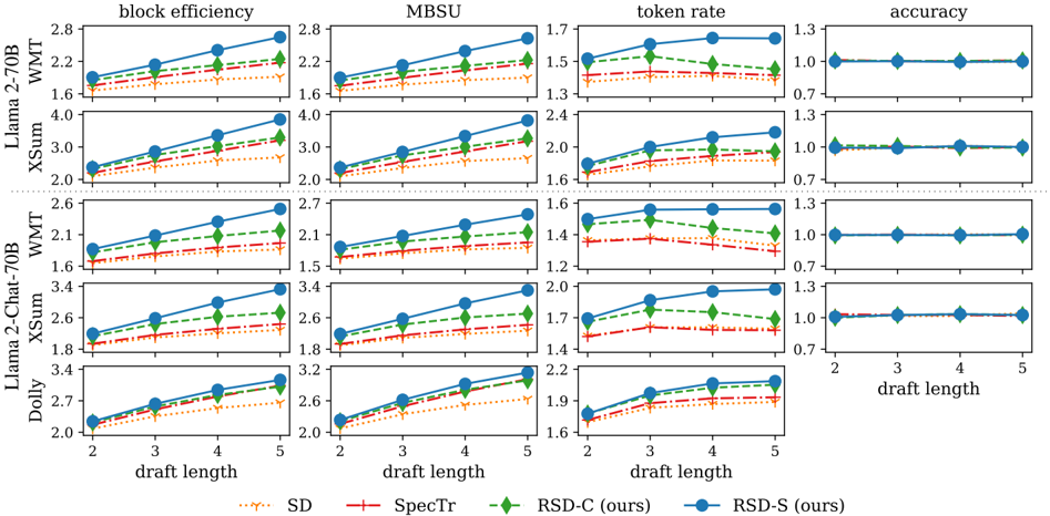
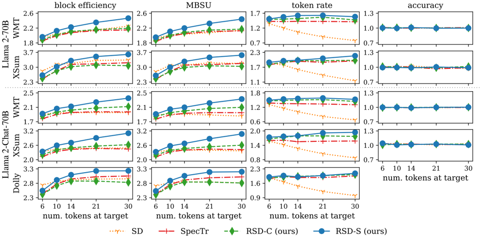
Figure 4. Block efficiency, MBSU, token rate and accuracy for various lengths ( 2 , 3 , 4 , 5 ) of draft sequences are given. We consider two target models, Llama 2-70B and Llama 2-Chat-70B, each of which has a corresponding smaller draft model for speculative decoding. All results are normalized by the corresponding numbers from auto-regressive decoding. RSD-S always outperforms SD, SpecTr and RSD-C. All methods including auto-regressive decoding show similar accuracy for WMT and XSum.
<details>
<summary>Image 4 Details</summary>
### Visual Description
## Line Chart: Performance Metrics vs. Draft Length for Different Models
### Overview
The image presents a series of four line charts, each displaying the relationship between "draft length" (x-axis) and four different performance metrics: "block efficiency", "MBSU", "token rate", and "accuracy" (y-axis). The charts compare the performance of five different models: "Llama 2-70B WMT", "Llama 2-Chat-70B XSum", "Llama 2-Chat-70B WMT", "Dolly", and "Llama 2-Chat-70B XSum". Each model's performance is represented by a different colored line.
### Components/Axes
* **X-axis:** "draft length" ranging from 2 to 5.
* **Y-axis:** Each chart has a different y-axis scale:
* "block efficiency": 1.6 to 2.8
* "MBSU": 2.8 to 4.0
* "token rate": 1.4 to 2.4
* "accuracy": 0.7 to 1.3
* **Models (Lines):**
* SD (dotted orange)
* Spectr (dashed red)
* RSD-C (ours) (dashed green)
* RSD-S (ours) (solid blue)
* **Legend:** Located at the bottom of the image, identifying the color and style of each line.
### Detailed Analysis or Content Details
**1. Block Efficiency Chart:**
* **SD (orange, dotted):** Line is relatively flat, starting at approximately 1.7 and ending around 1.8.
* **Spectr (red, dashed):** Line slopes upward, starting at approximately 1.8 and ending around 2.1.
* **RSD-C (green, dashed):** Line slopes upward, starting at approximately 1.9 and ending around 2.3.
* **RSD-S (blue, solid):** Line slopes upward, starting at approximately 2.0 and ending around 2.5.
**2. MBSU Chart:**
* **SD (orange, dotted):** Line slopes upward, starting at approximately 2.8 and ending around 3.2.
* **Spectr (red, dashed):** Line slopes upward, starting at approximately 3.0 and ending around 3.4.
* **RSD-C (green, dashed):** Line slopes upward, starting at approximately 3.1 and ending around 3.6.
* **RSD-S (blue, solid):** Line slopes upward, starting at approximately 3.2 and ending around 3.8.
**3. Token Rate Chart:**
* **SD (orange, dotted):** Line is relatively flat, starting at approximately 1.4 and ending around 1.5.
* **Spectr (red, dashed):** Line slopes upward, starting at approximately 1.5 and ending around 1.7.
* **RSD-C (green, dashed):** Line slopes upward, starting at approximately 1.6 and ending around 1.9.
* **RSD-S (blue, solid):** Line slopes upward, starting at approximately 1.7 and ending around 2.1.
**4. Accuracy Chart:**
* **SD (orange, dotted):** Line is relatively flat, starting at approximately 1.0 and ending around 1.0.
* **Spectr (red, dashed):** Line is relatively flat, starting at approximately 1.1 and ending around 1.1.
* **RSD-C (green, dashed):** Line is relatively flat, starting at approximately 1.1 and ending around 1.1.
* **RSD-S (blue, solid):** Line is relatively flat, starting at approximately 1.1 and ending around 1.1.
### Key Observations
* Generally, increasing the "draft length" leads to improved "block efficiency", "MBSU", and "token rate" for all models.
* "RSD-S (ours)" consistently outperforms other models across all metrics, showing the steepest upward trends.
* "SD" exhibits the lowest performance across all metrics, with relatively flat lines indicating minimal improvement with increasing "draft length".
* "Accuracy" remains relatively stable across all models and draft lengths.
### Interpretation
The data suggests that increasing the "draft length" can positively impact the performance of language models in terms of "block efficiency", "MBSU", and "token rate". The "RSD-S (ours)" model demonstrates superior performance compared to other models, indicating its effectiveness in leveraging longer draft lengths. The relatively stable "accuracy" suggests that increasing "draft length" does not significantly affect the correctness of the generated output. The flat lines for "SD" suggest that this model does not benefit as much from increased draft length as the other models. The consistent performance of "RSD-S" across all metrics indicates a robust and well-optimized model. The charts provide a comparative analysis of different models and highlight the importance of draft length in optimizing language model performance.
</details>
## 5. Experiments
We evaluate RSD-C and RSD-S together with our baselines including speculative decoding (SD) (Chen et al., 2023; Leviathan et al., 2023) and SpecTr (Sun et al., 2023), where a single draft model is assumed 4 . We consider the following perspectives during our experiments: ( Exp1 ) How will the performance be affected by the length of draft sequences ? ( Exp2 ) How will the performance be affected by the target computational budget , i.e., the number of tokens processed at the target model? While ( Exp1 ) has been frequently investigated by existing tree-based speculative decoding methods (Sun et al., 2023; Miao et al., 2023), ( Exp2 ) has not been considered in prior works but has practical importance when running the target model on resource-bounded devices.
Models. We consider the following target models; Llama 2 and Llama 2-Chat (Touvron et al., 2023) with 7B , 13B and 70B parameters; OPT (Zhang et al., 2022) with 13B , 30B and 66B parameters. Each class of target models adopts corresponding draft model; see Appendix C.1. In this section, we only present Llama 2-70B and Llama 2-Chat-70B results, and other results (Llama 2 with other sizes and OPT) can be found in Appendix C.4.
Tasks. Our methods and baselines are evaluated for WMT 18-DeEn (Bojar et al., 2018, translation) and XSum (Narayan et al., 2018, summarization) for each target
4 We exclude SpecInfer (Miao et al., 2023) from our baselines since it uses multiple draft models.
model, while we report accuracy scores (BLEU for WMT and ROUGE-2 for XSum) to confirm if the target model's distribution is recovered; DatabricksDolly -15k (Conover et al., 2023, question and answering) is used only for Llama 2-Chat without accuracy evaluation. We use temperature 0.3 for both XSum and WMT and 1.0 for Dolly, where we further apply nucleus (topp ) sampling (Holtzman et al., 2019) with p = 0 . 95 for Dolly.
Performance metrics. We evaluate block efficiency (Leviathan et al., 2023), Memory-Bound Speed-Up ( MBSU ) (Zhou et al., 2023) and token rate (tokens/sec) on A100 GPUs; see Appendix C.2 for details.
## 5.1. (Exp 1) Fixed draft sequence length
We fix (maximum) draft sequence length as the value in { 2 , 3 , 4 , 5 } and evaluate our methods and baselines, which is summarized in Figure 4 . Regarding the tree structures of each decoding methods, we let both SpecTr and RSD-S always use draft-token trees, the size of which is smaller than or equal to that of RSD-C's tree; see Appendix C.3.1 for details. Our results show that tree-based methods (SpecTr, RSD-C and RSD-S) always outperform SD in terms of block efficiency and MBSU, whereas token rates for SpecTr and RSD-C can be lower than that for SD; this is since block efficiencies for both SpecTr and RSD-C are relatively low and there is additional computational overhead to process the tree. On the other hand, RSD-S strictly outperforms both SD and SpecTr for all performance metrics , showing
Figure 5. Block efficiency, MBSU, token rate and accuracy for various target computational budgets (the numbers 6 , 10 , 14 , 21 , 30 of draft tokens processed at the target model) are given. We consider two target models, Llama 2-70B and Llama 2-Chat-70B, each of which has a corresponding smaller draft model for speculative decoding. All results are normalized by the corresponding numbers from auto-regressive decoding. RSD-S outperforms SD, SpecTr and RSD-C in the majority of cases. All methods including auto-regressive decoding show similar accuracy for both WMT and XSum.
<details>
<summary>Image 5 Details</summary>
### Visual Description
## Chart: Performance Metrics vs. Number of Tokens at Target
### Overview
This image presents a series of four line charts, arranged in a 2x2 grid, comparing the performance of different models (Llama 2-70B XSum, Llama 2-Chat-70B XSum, Llama 2-70B WMT, Llama 2-Chat-70B WMT, and Dolly) across four metrics: Block Efficiency, MBSU, Token Rate, and Accuracy. Each chart displays the performance of each model as a function of the "num. tokens at target" ranging from 6 to 30. Four different methods are being compared: SD, Spectr, RSD-C (ours), and RSD-S (ours).
### Components/Axes
* **X-axis (all charts):** "num. tokens at target" with markers at 6, 10, 14, 21, and 30.
* **Y-axis (Block Efficiency & MBSU charts):** Ranges from approximately 1.7 to 3.7. Labeled "block efficiency" and "MBSU" respectively.
* **Y-axis (Token Rate chart):** Ranges from approximately 0.7 to 2.3. Labeled "token rate".
* **Y-axis (Accuracy chart):** Ranges from approximately 0.7 to 1.3. Labeled "accuracy".
* **Legend:** Located at the top-right of the image. Contains the following entries with corresponding colors:
* SD (dotted orange line)
* Spectr (solid red line)
* RSD-C (ours) (solid green line)
* RSD-S (ours) (solid blue line)
* **Rows:** Each row represents a different model:
* Llama 2-70B XSum
* Llama 2-Chat-70B XSum
* Llama 2-70B WMT
* Llama 2-Chat-70B WMT
* Dolly
### Detailed Analysis or Content Details
**Block Efficiency Chart:**
* **Llama 2-70B XSum:** SD shows a decreasing trend from ~2.5 to ~1.8. Spectr is relatively flat around ~2.1. RSD-C (ours) increases from ~1.8 to ~2.3. RSD-S (ours) increases from ~1.9 to ~2.4.
* **Llama 2-Chat-70B XSum:** SD decreases from ~3.5 to ~2.5. Spectr is relatively flat around ~2.8. RSD-C (ours) increases from ~2.4 to ~3.1. RSD-S (ours) increases from ~2.6 to ~3.3.
* **Llama 2-70B WMT:** SD decreases from ~2.5 to ~2.0. Spectr is relatively flat around ~2.2. RSD-C (ours) increases from ~2.1 to ~2.5. RSD-S (ours) increases from ~2.2 to ~2.6.
* **Llama 2-Chat-70B WMT:** SD decreases from ~3.2 to ~2.6. Spectr is relatively flat around ~2.8. RSD-C (ours) increases from ~2.6 to ~3.2. RSD-S (ours) increases from ~2.8 to ~3.3.
* **Dolly:** SD decreases from ~3.3 to ~2.3. Spectr is relatively flat around ~2.8. RSD-C (ours) increases from ~2.3 to ~2.8. RSD-S (ours) increases from ~2.5 to ~3.1.
**MBSU Chart:**
* **Llama 2-70B XSum:** SD decreases from ~2.5 to ~1.8. Spectr is relatively flat around ~2.1. RSD-C (ours) increases from ~1.8 to ~2.3. RSD-S (ours) increases from ~1.9 to ~2.4.
* **Llama 2-Chat-70B XSum:** SD decreases from ~3.5 to ~2.5. Spectr is relatively flat around ~2.8. RSD-C (ours) increases from ~2.4 to ~3.1. RSD-S (ours) increases from ~2.6 to ~3.3.
* **Llama 2-70B WMT:** SD decreases from ~2.5 to ~2.0. Spectr is relatively flat around ~2.2. RSD-C (ours) increases from ~2.1 to ~2.5. RSD-S (ours) increases from ~2.2 to ~2.6.
* **Llama 2-Chat-70B WMT:** SD decreases from ~3.2 to ~2.6. Spectr is relatively flat around ~2.8. RSD-C (ours) increases from ~2.6 to ~3.2. RSD-S (ours) increases from ~2.8 to ~3.3.
* **Dolly:** SD decreases from ~3.3 to ~2.3. Spectr is relatively flat around ~2.8. RSD-C (ours) increases from ~2.3 to ~2.8. RSD-S (ours) increases from ~2.5 to ~3.1.
**Token Rate Chart:**
* **Llama 2-70B XSum:** SD decreases from ~1.7 to ~0.7. Spectr decreases from ~1.4 to ~0.7. RSD-C (ours) is relatively flat around ~1.7. RSD-S (ours) is relatively flat around ~1.9.
* **Llama 2-Chat-70B XSum:** SD decreases from ~1.7 to ~0.7. Spectr decreases from ~1.4 to ~0.7. RSD-C (ours) is relatively flat around ~1.7. RSD-S (ours) is relatively flat around ~1.9.
* **Llama 2-70B WMT:** SD decreases from ~1.7 to ~0.7. Spectr decreases from ~1.4 to ~0.7. RSD-C (ours) is relatively flat around ~1.7. RSD-S (ours) is relatively flat around ~1.9.
* **Llama 2-Chat-70B WMT:** SD decreases from ~1.7 to ~0.7. Spectr decreases from ~1.4 to ~0.7. RSD-C (ours) is relatively flat around ~1.7. RSD-S (ours) is relatively flat around ~1.9.
* **Dolly:** SD decreases from ~1.7 to ~0.7. Spectr decreases from ~1.4 to ~0.7. RSD-C (ours) is relatively flat around ~1.7. RSD-S (ours) is relatively flat around ~1.9.
**Accuracy Chart:**
* **Llama 2-70B XSum:** SD is relatively flat around ~1.0. Spectr is relatively flat around ~1.0. RSD-C (ours) is relatively flat around ~1.1. RSD-S (ours) is relatively flat around ~1.2.
* **Llama 2-Chat-70B XSum:** SD is relatively flat around ~1.0. Spectr is relatively flat around ~1.0. RSD-C (ours) is relatively flat around ~1.1. RSD-S (ours) is relatively flat around ~1.2.
* **Llama 2-70B WMT:** SD is relatively flat around ~1.0. Spectr is relatively flat around ~1.0. RSD-C (ours) is relatively flat around ~1.1. RSD-S (ours) is relatively flat around ~1.2.
* **Llama 2-Chat-70B WMT:** SD is relatively flat around ~1.0. Spectr is relatively flat around ~1.0. RSD-C (ours) is relatively flat around ~1.1. RSD-S (ours) is relatively flat around ~1.2.
* **Dolly:** SD is relatively flat around ~1.0. Spectr is relatively flat around ~1.0. RSD-C (ours) is relatively flat around ~1.1. RSD-S (ours) is relatively flat around ~1.2.
### Key Observations
* SD and Spectr generally perform worse than RSD-C and RSD-S in terms of Block Efficiency and MBSU, showing a decreasing trend as the number of tokens at target increases.
* RSD-C and RSD-S consistently show an increasing trend in Block Efficiency and MBSU as the number of tokens at target increases.
* Token Rate decreases for SD and Spectr as the number of tokens at target increases, while RSD-C and RSD-S remain relatively stable.
* Accuracy remains relatively stable across all methods and token counts.
* RSD-S consistently outperforms RSD-C across all metrics.
### Interpretation
The data suggests that the RSD-C and RSD-S methods are more robust and scalable than SD and Spectr, particularly as the number of tokens at target increases. The increasing Block Efficiency and MBSU with RSD-C and RSD-S indicate improved resource utilization and potentially better compression or processing efficiency. The stable Token Rate for RSD-C and RSD-S suggests they maintain a consistent processing speed regardless of the input size. The relatively flat accuracy curves indicate that increasing the number of tokens at target does not significantly impact the accuracy of any of the methods. The consistent outperformance of RSD-S over RSD-C suggests that the modifications implemented in RSD-S are beneficial. The decreasing performance of SD and Spectr with increasing token count could indicate limitations in their ability to handle larger inputs effectively. The consistent performance of all methods on the accuracy metric suggests that the primary differences lie in efficiency and scalability rather than fundamental accuracy.
</details>
the superiority of RSD-S over our baselines and the importance of early-truncating unlikely draft sequences. We also observe that there is no strong correlation between MBSU and token rate; this is since A100 GPUs used to measure token rates are not memory-bound. Furthermore, token rates in many cases are shown to decrease as the length of draft-token sequence becomes higher, which is due to the increased computation overhead to execute draft models with the longer draft sequence; however, one needs to be cautious since this result may not generally hold since token rate is hugely affected by the efficiency of software implementation and the devices which we execute the methods on. Finally, in WMT and XSum, BLEU and ROUGE-2 scores are similar across different methods, respectively, which implies that all methods recover the distributions of target LLMs.
## 5.2. ( Exp2 ) Fixed target computational budget
We select target computational budget, i.e., the number of draft tokens processed at the target model in parallel for each speculative decoding iteration, among values in { 6 , 10 , 14 , 21 , 30 } and evaluate our proposed methods and baselines; we summarize the results in Figure 5 and describe tree structures in Appendix C.3.2. While RSD-S achieves higher block efficiency and MBSU than SD and SpecTr in most cases, SD beats RSD-C in the relatively low budget regime, e.g., { 6 , 10 } with Llama 2-70B and XSum, and { 6 }
with Llama 2-Chat-70B and Dolly. We believe that our draft models are well-aligned with corresponding target models for those cases (from the observation that block efficiencies of SD close to 3.0, which are significantly higher than the numbers in other cases, are achieved), and increasing the depth rather than the width of the tree could quickly increase the acceptance rate in such cases. In the high budget regime, on the other hand, RSD-S beats SD for both block efficiency and MBSU. In terms of token rate, RSD-S strictly outperforms our baselines, whereas SD's token rate severely decreases for higher target computation budgets due to the computational overhead caused by the draft model's autoregressive decoding with the longer draft sequence.
## 6. Conclusion
We present RSD algorithms, a novel tree-based speculative decoding method leveraging the full diversifiability of the draft-token tree; RSD-C efficiently samples draft tokens without replacement via Gumbel-Topk trick, while RSD-S uses Stochastic Beam Search and samples drafttoken sequences without replacement. We also propose recursive rejection sampling that can verify the tree built by the sampling-without-replacement process and recovers the exact target model distribution. We show that RSD outperforms the baselines in most cases, supporting the importance of diverse drafting when accelerating LLM inference.
## References
- Achiam, J., Adler, S., Agarwal, S., Ahmad, L., Akkaya, I., Aleman, F. L., Almeida, D., Altenschmidt, J., Altman, S., Anadkat, S., et al. GPT-4 technical report. arXiv preprint arXiv:2303.08774 , 2023.
- Bojar, O. r., Federmann, C., Fishel, M., Graham, Y., Haddow, B., Huck, M., Koehn, P., and Monz, C. Findings of the 2018 conference on machine translation (wmt18). In Proceedings of the Third Conference on Machine Translation, Volume 2: Shared Task Papers , pp. 272-307, Belgium, Brussels, October 2018. Association for Computational Linguistics. URL http://www . aclweb . org/ anthology/W18-6401 .
- Brown, T., Mann, B., Ryder, N., Subbiah, M., Kaplan, J. D., Dhariwal, P., Neelakantan, A., Shyam, P., Sastry, G., Askell, A., et al. Language models are few-shot learners. Advances in Neural Information Processing Systems (NeurIPS) , 33:1877-1901, 2020.
- Cai, T., Li, Y., Geng, Z., Peng, H., and Dao, T. Medusa: Simple framework for accelerating llm generation with multiple decoding heads. https://github . com/ FasterDecoding/Medusa , 2023.
- Cai, T., Li, Y., Geng, Z., Peng, H., Lee, J. D., Chen, D., and Dao, T. Medusa: Simple llm inference acceleration framework with multiple decoding heads. arXiv preprint arXiv:2401.10774 , 2024.
- Chen, C., Borgeaud, S., Irving, G., Lespiau, J.-B., Sifre, L., and Jumper, J. Accelerating large language model decoding with speculative sampling. arXiv preprint arXiv:2302.01318 , 2023.
- Conover, M., Hayes, M., Mathur, A., Xie, J., Wan, J., Shah, S., Ghodsi, A., Wendell, P., Zaharia, M., and Xin, R. Free dolly: Introducing the world's first truly open instruction-tuned llm, 2023. URL https://www . databricks . com/blog/2023/ 04/12/dolly-first-open-commerciallyviable-instruction-tuned-llm .
- Fu, Y., Bailis, P., Stoica, I., and Zhang, H. Breaking the sequential dependency of LLM inference using lookahead decoding, November 2023. URL https://lmsys . org/blog/2023-11-21lookahead-decoding/ .
- Holtzman, A., Buys, J., Du, L., Forbes, M., and Choi, Y. The curious case of neural text degeneration. arXiv preprint arXiv:1904.09751 , 2019.
- Jiang, A. Q., Sablayrolles, A., Mensch, A., Bamford, C., Chaplot, D. S., Casas, D. d. l., Bressand, F., Lengyel, G., Lample, G., Saulnier, L., et al. Mistral 7B. arXiv preprint arXiv:2310.06825 , 2023.
- Kim, S., Mangalam, K., Malik, J., Mahoney, M. W., Gholami, A., and Keutzer, K. Big little transformer decoder. arXiv preprint arXiv:2302.07863 , 2023.
- Kool, W., Van Hoof, H., and Welling, M. Stochastic beams and where to find them: The Gumbel-Topk trick for sampling sequences without replacement. In Proceedings of the 36th International Conference on Machine Learning (ICML) , pp. 3499-3508. PMLR, 2019.
- Leviathan, Y., Kalman, M., and Matias, Y. Fast inference from transformers via speculative decoding. In Proceedings of the 40th International Conference on Machine Learning (ICML) , 2023.
- Miao, X., Oliaro, G., Zhang, Z., Cheng, X., Wang, Z., Wong, R. Y. Y., Chen, Z., Arfeen, D., Abhyankar, R., and Jia, Z. SpecInfer: Accelerating generative LLM serving with speculative inference and token tree verification. arXiv preprint arXiv:2305.09781 , 2023.
- Narayan, S., Cohen, S. B., and Lapata, M. Don't give me the details, just the summary! Topic-aware convolutional neural networks for extreme summarization. arXiv preprint arXiv:1808.08745 , 2018.
- Shazeer, N. Fast transformer decoding: One write-head is all you need. arXiv preprint arXiv:1911.02150 , 2019.
- Sun, Z., Suresh, A. T., Ro, J. H., Beirami, A., Jain, H., and Yu, F. SpecTr: Fast speculative decoding via optimal transport. In Advances in Neural Information Processing Systems (NeurIPS) , 2023.
- Touvron, H., Martin, L., Stone, K., Albert, P., Almahairi, A., Babaei, Y., Bashlykov, N., Batra, S., Bhargava, P., Bhosale, S., et al. Llama 2: Open foundation and finetuned chat models. arXiv preprint arXiv:2307.09288 , 2023.
- Vaswani, A., Shazeer, N., Parmar, N., Uszkoreit, J., Jones, L., Gomez, A. N., Kaiser, Ł., and Polosukhin, I. Attention is all you need. Advances in Neural Information Processing Systems (NeurIPS) , 30, 2017.
- Vieira, T. Gumbel-max trick and weighted reservoir sampling. 2014. URL https: //timvieira . github . io/blog/post/2014/ 08/01/gumbel-max-trick-andweightedreservoir-sampling/ .
- Villani, C. et al. Optimal transport: old and new , volume 338. Springer, 2009.
- Xia, H., Yang, Z., Dong, Q., Wang, P., Li, Y., Ge, T., Liu, T., Li, W., and Sui, Z. Unlocking efficiency in large language model inference: A comprehensive survey of speculative decoding. arXiv preprint arXiv:2401.07851 , 2024.
- Xiao, Y., Wu, L., Guo, J., Li, J., Zhang, M., Qin, T., and Liu, T.-y. A survey on non-autoregressive generation for neural machine translation and beyond. IEEE Transactions on Pattern Analysis and Machine Intelligence , 2023.
- Zhang, S., Roller, S., Goyal, N., Artetxe, M., Chen, M., Chen, S., Dewan, C., Diab, M., Li, X., Lin, X. V., et al. OPT: Open pre-trained transformer language models. arXiv preprint arXiv:2205.01068 , 2022.
- Zhou, Y., Lyu, K., Rawat, A. S., Menon, A. K., Rostamizadeh, A., Kumar, S., Kagy, J.-F., and Agarwal, R. Distillspec: Improving speculative decoding via knowledge distillation. arXiv preprint arXiv:2310.08461 , 2023.
## A. Theorems and proofs
## A.1. Proof of Theorem 3.1
Theorem 3.1 (Recursive rejection sampling recovers target distribution) . The random variable Z ∈ X defining recursive rejection sampling rule (4) follows the target distribution q , i.e.,
$$\Pr \left \{ Z = z \right \} = q ( z ) , z \in \mathcal { X } .$$
Proof. We remain a sketch of the proof here and the formal proof is given in the next paragraph. We first consider the case where ˆ X (1) , ..., ˆ X ( K -1) are rejected and see whether we accept ˆ X ( K ) or not; we either accept ˆ X ( K ) with probability Θ ( K ) in (3) or sample a new token Y ∼ q ( K +1) ( ·| ˆ X (1: K -1) ) when all draft tokens are rejected. Since q ( K +1) is the residual distribution from q ( K ) , one can regard it as the simple sampling by Chen et al. (2023) and Leviathan et al. (2023), which recovers q ( K ) . The same idea is applied to ˆ X ( K -1) , ..., ˆ X (1) in the reversed order until we recover q = q (1) at the end.
Let us desribe the formal proof. From the definition of recursive rejection sampling (4), we have
<!-- formula-not-decoded -->
It can be shown that the following equality holds for each k :
$$\Sigma _ { 2 , k - 1 } = \Sigma _ { 1 , k } + \Sigma _ { 2 , k } .$$
Let us first consider k = K , then,
$$& \text {$\Sigma_{1,K}+ \Sigma_{2,K}$} \\ & = \sum _ { x ^ { ( 1 ) } , \dots , x ^ { ( K - 1 ) } } \Pr \left \{ \hat { X } ^ { ( 1 \colon K - 1 ) } = x ^ { ( 1 \colon K - 1 ) } \right \} \times \Pr \left \{ A ^ { ( 1 \colon K - 1 ) } = \text {rej} ^ { K - 1 } , \hat { X } ^ { ( K ) } = z , A ^ { ( K ) } = \text {acc} \Big | \hat { X } ^ { ( 1 \colon K - 1 ) } = x ^ { ( 1 \colon K - 1 ) } \right \} \\ & + \sum _ { x ^ { ( 1 ) } , \dots , x ^ { ( K ) } } \Pr \left \{ \hat { X } ^ { ( 1 \colon K ) } = x ^ { ( 1 \colon K ) } \right \} \times \Pr \left \{ A ^ { ( 1 \colon K ) } = \text {rej} ^ { K } , \hat { X } ^ { ( K + 1 ) } = z \Big | \hat { X } ^ { ( 1 \colon K ) } = x ^ { ( 1 \colon K ) } \right \} \\ & = \sum _ { x ^ { ( 1 ) } , \dots , x ^ { ( K - 1 ) } } \Pr \left \{ \hat { X } ^ { ( 1 \colon K - 1 ) } = x ^ { ( 1 \colon K - 1 ) } \right \} \Big ( \underbrace { \Pr \left \{ A ^ { ( 1 \colon K - 1 ) } = \text {rej} ^ { K - 1 } , \hat { X } ^ { ( K ) } = z , A ^ { ( K ) } = \text {acc} \Big | \hat { X } ^ { ( 1 \colon K - 1 ) } = x ^ { ( 1 \colon K - 1 ) } \right \} } _ { = \colon T _ { 2 } ( K ) } \\ & \quad + \underbrace { \sum _ { x ^ { ( K ) } } \Pr \left \{ \hat { X } ^ { ( K ) } = x ^ { ( K ) } \Big | \hat { X } ^ { ( 1 \colon K - 1 ) } = x ^ { ( 1 \colon K - 1 ) } \right \} \times \Pr \left \{ A ^ { ( 1 \colon K ) } = \text {rej} ^ { K } , \hat { X } ^ { ( K + 1 ) } = z \Big | \hat { X } ^ { ( 1 \colon K ) } = x ^ { ( 1 \colon K ) } \right \} } _ { = \colon T _ { 2 } ( K ) } \right ) .
<text><loc_66><loc_464><loc_196><loc_484>One can represent $^{T$_{1,K}$}$and$^{T$_{2,K}$}$as follows:</text>
</doctag>$$
One can represent T 1 ,K and T 2 ,K as follows:
$$T _ { 1 , K } & = \Pr \left \{ A ^ { ( 1 \colon K - 1 ) } = \text {re} j ^ { K - 1 } \Big | \hat { X } ^ { ( 1 \colon K - 1 ) } = x ^ { ( 1 \colon K - 1 ) } \right \} \\ & \quad \times \Pr \left \{ \hat { X } ^ { ( K ) } = z \Big | \hat { X } ^ { ( 1 \colon K - 1 ) } = x ^ { ( 1 \colon K - 1 ) } \right \} \times \text {Pr} \left \{ A ^ { ( K ) } = \text {acc} \Big | \hat { X } ^ { ( 1 \colon K ) } = ( x ^ { ( 1 \colon K - 1 ) } , z ) \right \} \\ & = \Pr \left \{ A ^ { ( 1 \colon K - 1 ) } = \text {re} j ^ { K - 1 } \Big | \hat { X } ^ { ( 1 \colon K - 1 ) } = x ^ { ( 1 \colon K - 1 ) } \right \} p ^ { ( K ) } ( z | x ^ { ( 1 \colon K - 1 ) } ) \min \left \{ 1 , \frac { q ^ { ( K ) } ( z | x ^ { ( 1 \colon K - 2 ) } ) } { p ^ { ( K ) } ( z | x ^ { ( 1 \colon K - 1 ) } ) } \right \} \\ & = \Pr \left \{ A ^ { ( 1 \colon K - 1 ) } = \text {re} j ^ { K - 1 } \Big | \hat { X } ^ { ( 1 \colon K - 1 ) } = x ^ { ( 1 \colon K - 1 ) } \right \} \min \left \{ p ^ { ( K ) } ( z | x ^ { ( 1 \colon K - 1 ) } ) , q ^ { ( K ) } ( z | x ^ { ( 1 \colon K - 2 ) } ) \right \} ,$$
<!-- formula-not-decoded -->
Therefore, we have
$$& T _ { 1 , K } + T _ { 2 , K } \\ & = \Pr \left \{ A ^ { ( 1 \colon K - 1 ) } = \text {re} j ^ { K - 1 } \Big | \hat { X } ^ { ( 1 \colon K - 1 ) } = x ^ { ( 1 \colon K - 1 ) } \right \} \\ & \quad \times \left ( \min \left \{ p ^ { ( K ) } ( z | x ^ { ( 1 \colon K - 1 ) } ) , q ^ { ( K ) } ( z | x ^ { ( 1 \colon K - 2 ) } ) \right \} + \max \left \{ 0 , q ^ { ( K ) } ( z | x ^ { ( 1 \colon K - 2 ) } ) - p ^ { ( K ) } ( z | x ^ { ( 1 \colon K - 1 ) } ) \right \} \right ) \\ & = \Pr \left \{ A ^ { ( 1 \colon K - 1 ) } = \text {re} j ^ { K - 1 } \Big | \hat { X } ^ { ( 1 \colon K - 1 ) } = x ^ { ( 1 \colon K - 1 ) } \right \} q ^ { ( K ) } ( z | x ^ { ( 1 \colon K - 2 ) } ) \\ & = \Pr \left \{ A ^ { ( 1 \colon K - 1 ) } = \text {re} j ^ { K - 1 } , \tilde { X } ^ { ( K ) } = z \Big | \hat { X } ^ { ( 1 \colon K - 1 ) } = x ^ { ( 1 \colon K - 1 ) } \right \} ,$$
where we define a random variable ˜ X ( K ) such that
$$P r \left \{ \tilde { X } ^ { ( K ) } = z \right | \hat { X } ^ { ( 1 \colon K - 1 ) } = x ^ { ( 1 \colon K - 1 ) } \right \} \colon = q ^ { ( K ) } ( z | x ^ { ( 1 \colon K - 1 ) } ) ,$$
which leads to
$$& \Sigma _ { 1 , K } + \Sigma _ { 2 , K } \\ & = \sum _ { x ^ { ( 1 ) } , \dots , x ^ { ( K - 1 ) } } \Pr \left \{ \hat { X } ^ { ( 1 \colon K - 1 ) } = x ^ { ( 1 \colon K - 1 ) } \right \} ( T _ { 1 , K } + T _ { 2 , K } ) \\ & = \sum _ { x ^ { ( 1 ) } , \dots , x ^ { ( K - 1 ) } } \Pr \left \{ \hat { X } ^ { ( 1 \colon K - 1 ) } = x ^ { ( 1 \colon K - 1 ) } \right \} \times \Pr \left \{ A ^ { ( 1 \colon K - 1 ) } = \text {rej} ^ { K - 1 } , \tilde { X } ^ { ( K ) } = z \Big | \hat { X } ^ { ( 1 \colon K - 1 ) } = x ^ { ( 1 \colon K - 1 ) } \right \} \\ & = \Pr \left \{ A ^ { ( 1 \colon K - 1 ) } = \text {rej} ^ { K - 1 } , \tilde { X } ^ { ( K ) } = z \right \} \\ & = \Sigma _ { 2 , K - 1 } .$$
Since the same derivation can be done for k = 2 , ..., K -1 , we have
$${ P r } \left \{ Z = z \right \} = \sum _ { k = 1 } ^ { K } \Sigma _ { 1 , k } + \Sigma _ { 2 , K } = \sum _ { k = 1 } ^ { K - 1 } \Sigma _ { 1 , k } + \Sigma _ { 2 , K - 1 } = \cdots = \Sigma _ { 1 , 1 } + \Sigma _ { 2 , 1 } = q ( z ) ,$$
where the last equality holds from the derivation of original speculative decoding by (Chen et al., 2023; Leviathan et al., 2023).
## A.2. Proof of Theorem 3.2
Theorem 3.2 (Tokens from the same sequence follow sampling without replacement in RSD-S) . In RSD-S, any non-empty subsequence of the sequence ˆ X (1) l +1 , ..., ˆ X ( W ) l +1 of draft tokens (from O (1) l +1 , ..., O ( W ) l +1 in (12) ) such that each element of the subsequence has the same parent τ ( k ) l follows sampling without replacement from p ( ·| τ ( k ) l ) .
Proof. For fixed τ ( k ) l , consider a sequence of tokens
$$\bar { X } _ { l + 1 } ^ { ( k ) } \colon = \underset { x \in \mathcal { X } } { \arg s o r t } \psi _ { l } ( \tau _ { l } ^ { ( k ) } , x ) = \underset { x \in \mathcal { X } } { \arg s o r t } \tilde { \phi } _ { l } ( \tau _ { l } ^ { ( k ) } , x ) ,$$
where the last equality holds since T in (10) is monotonically increasing w.r.t. ˜ ϕ l ( τ ( k ) l , · ) for fixed τ ( k ) l . Thus, ¯ X ( k ) l +1 can be seen as samples from p ( ·| τ ( k ) l ) without replacement.
For a lengthl k subsequence o ( k ) l +1 of ( O (1) l +1 , ..., O ( W ) l +1 ) in (12), where each element of the subsequence have τ ( k ) l as its parent, the token sequence in o ( k ) l +1 is a subsequence of ¯ X ( k ) l +1 , i.e., those tokens are topl k samples without replacement from p ( ·| τ ( k ) l ) .
## B. Algorithm
## B.1. Recursive Speculative Decoding with Constant Branching Factors (RSD-C)
## Algorithm 2 Recursive Speculative Decoding with Constant Branching Factors (RSD-C)
- 10:
- 11:
- 12:
- 13:
```
B.1. Recursive Speculative Decoding with Constant Branching Factors (RSD-C)
Algorithm 2 Recursive Speculative Decoding with Constant Branching Factors (RSD-C)
1: Input: The length L$_draft of draft sequences (depth of the draft tree), a sequence x$_input of input tokens, a list
b := [b$_0,...,b$_draft$_-1] of constant branching factors in the draft tree, the maximum length L$_output of the output
sequence.
2: // Get the length of the input sequence.
L$_input ← GetLength(x$_input).
3: // Initialize empty KV caches for draft and target models.
C$_draft ← , C$_target ← .
4: while L$_input < L$_output do
5: // (STEP 1) Create a draft tree by using the draft model.
T, x$_input, C$_draft, M, id$_position, L$_num_nodes ← CreateDraftTreeConst(x$_input, C$_draft, b, L$_draft).
6: // (STEP 2) Evaluate draft tokens by using the target model.
// - Apply M to the right below corner of attention weights.
// - The target log probability Φ$_target is a GetLength(x$_input) × N$_vocab tensor.
// - N$_vocab is the vocabulary size.
7: // Convert the log probability tensor into the list of log probabilities
for each level of the tree.
L$_log_probs_target ← SplitTensor(Φ$_target[-Sum(L$_num_nodes) :,:],L$_num_nodes, dim = 0)
8: // (STEP 3) Run Recursive Rejection Sampling for each level of the tree.
x$_accepted, x$_last, id$_accepted flat node ← RecursiveRejectionSampling(T, L$_log_probs_target)
9: // (STEP 4) Use KV caches that are accepted, and prepare for the next round.
C$_draft, C$_target ← FilterKVCache(C$_draft, C$_target, L$_input, id$_accepted flat node)
10: x$_input ← Concat([x$_input[:L$_input],x$_accepted,x$_last])
11: L$_input ← GetLength(x$_input)
12: end while
```
## Algorithm 3 CreateDraftTreeConst ( x input , C draft , b , L draft )
```
Recursive Speculative Decoding: Accelerating LLM Inference via Sampling Without Replacement
-----------------------------------------------------------------------------
Algorithm 3 CreateDraftTreeConst(xinput, Cdraft, b, Ldraft)
----------------------
1: Input: An input sequence xinput, the draft KV cache Cdraft, the branching factor b := [b0,...,bLdraft-1], the draft
length Ldraft
2: // Get the length of the input sequence.
Linput <-GetLength(xinput).
3: // Initialize lists for 1) draft log probabilities, 2) flattened node IDs, 3)
parent node ids (within each level of the draft tree), 4) draft tokens, 5)
numbers of nodes (for all levels of the tree), respectively.
Llog-probs-draft <- [], Lflat-node-ids <- [], Lparent-ids <- [], Ldraft-tokens <- [], Lnum-nodes <- [].
4: // Initialize a draft tree.
T <- (Llog-probs-draft, Lflat-node-ids, Lparent-ids, Ldraft-tokens).
5: // Set an empty attention mask, and position ids; inclusive for start and
exclusive for end.
M <- 0, id_position <- Arange(start = 0, end = Linput).
6: // Set the counter to check the number of nodes in the tree.
Ntree-prev <- 0, Ntree-curr <- 0.
7: // Set the number of nodes at the current level of the tree.
Nnodes <- 1, Lnum-nodes.append(Nnodes).
8: for ldraft = 0 to Ldraft - 1 do
9: // Apply M to the right below corner of attention weights.
10: // The draft log probability Pdraft is a GetLength(xinput) × Nvocab tensor.
11: // Nvocab is the vocabulary size.
12: Pdraft, Cdraft <- DraftModelForwardPass(xinput, Cdraft, id_position, M).
13: // Sample bLraft nodes without replacement, independently for Nnodes nodes.
14: // NOTE: Outputs are sorted w.r.t. the value of perturbed log probabilities and flattened.
15: xdraft, id_parent <- SampleWithGumbelTopK(Pdraft[-Nnodes :,:], bLraft).
16: // Update the input sequence of tokens.
17: xinput <- Concat([xinput, xdraft]).
18: // Get the number of newly added nodes.
19: Nnodes <- GetLength(xdraft).
20: // Build attention mask reflecting tree topology.
21: M <- BuildAttentionMask(M, id_parent, Nnodes, Ntree-prev, Ntree-curr).
22: // Update counters.
23: Ntree-prev <- Ntree-curr, Ntree-curr <- Ntree-curr + Nnodes.
24: // Update position IDs.
25: id_position <- Concat([id_position, (Linput + ldraft) x1, Nnodes]).
26: // Get node IDs considering the flattened draft tree.
27: // This is used to update KV caches.
28: idflat-node <- Arange(start = Linput + Ntree-prev, end = Linput + Ntree-curr).
29: // Update the lists of the tree.
30: Llog-probs-draft.append(Pdraft), Lflat-node-ids.append(id_flat-node), Lparent-ids.append(id_parent),
31: Ldraft-tokens.append(xdraft), Lnum-nodes.append(Nnodes).
32: end for
33: Output: T, xinput, Cdraft, M, id_position, Lnum-nodes.
```
## Algorithm 4 SampleWithGumbelTopK ( Φ , K )
- 1: Input: a N nodes × N vocab log probabilities Φ , the number K of desired samples without replacement. 2: // Sample a matrix where elements are i.i.d. standard Gumbel random variables. G ← [ g ij ] , g ij ← SampleStandardGumbel () , i = 0 , ..., N nodes -1 , j = 0 , ..., N vocab -1 . 3: // Perturb log probabilities with Gumbel random variables. ˜ Φ ← Φ + G . 4: // Get topK elements corresponding to the K largest perturb log probabilities. // Outputs are sorted (in each row) w.r.t. the values of perturbed log probabilities and flattened. x ← argtop ( K ) ( ˜ Φ , dim = -1) . flatten () . 5: // Set parent ids. id parent ← Concat ([0 · 1 K , 1 · 1 K , ..., ( N nodes -1) · 1 K ]) . 6: // When probability filtering methods(e.g., topp , topk ) were applied, filter some elements of x and id parent if corresponding log probability is equal to -∞ . 7: Output : x , id parent .
## Algorithm 5 BuildAttentionMask ( M , id parent , N nodes , N tree prev , N tree curr )
- 1: Input: previous attention mask M , parent node ids id parent for newly added nodes, the number N nodes of nodes newly added to the tree, the total number N tree prev of nodes in the previous-iteration tree, the total number N tree curr of nodes in the current-iteration tree.
```
added to the tree, the total number Ntree prev of nodes in the previous-iteration tree, the total number Ntree curr of nodes
in the current-iteration tree.
2: if M == then
3: // If the attention mask is empty, we initialize with zeros.
M ← 0$_{Nnodes}$×$N$_{nodes}$.
4: else
5: // If the attention mask exists, we zero-pad.
M ← ZeroPadding(M , right = N$_{nodes}$ , bottom = N$_{nodes}$ ).
6: for i = 0 to N$_{nodes}$ - 1 do
7: // Copy the row about paraent nodes to the row about child nodes.
M[Ntree curr + i, :] ← M[Ntree prev + id$_parent[i], :].
8: end for
9: end if
10: // Set diagonal elements equal to 1.
M ← M .fill diagonal(1)
11: Output: the new attention mask M.
```
## Algorithm 6 RecursiveRejectionSampling ( T , L log probs target )
̸
```
RecursiveSpeculativeDecoding: Accelerating LLM Inference via Sampling Without Replacement
==============================================================================
Algorithm 6 RecursiveRejectionSampling(T,Llog_probs target)
-----------------------------------------------------------------------------
1: Input: the draft tree T, the list Llog_probs target of target log probabilities
2: // Get lists from the draft tree.
3: Llog_probs_draft, Lflat_node_ids, Lparent_ids, Ldraft_tokens <-T
4: // Set the current node id.
5: inode <- 0
6: // Initialize the lists to store accepted draft tokens and flattened node ids
(for KV cache update).
Laccepted_draft_tokens <- [],Laccepted_flat_node_ids <- [].
5: for ldraft = 0 to Ldraft - 1 do
6: // Get log probabilities at the current node.
7: // Both are 1 x Nvocab tensors, where Nvocab is the vocabulary size.
8: Draft <- Llog_probs_draft[ldraft][inode : (inode + 1), :] ,Ttarget <- Llog_probs_target[ldraft][inode : (inode + 1),:]
7: // Get draft tokens, flattened node IDs, parent IDs at the current level.
8: xdraft <- Ldraft_tokens[ldraft], idflat_node_ids[ldraft], idparent <- Lparent_ids[ldraft]
9: // Initialize an acceptance indicator as False.
10: accept <- False
11: for i in idparent do
12: if i # inode then
13: continue
14: end if
15: // Get the current draft token.
16: xd <- xdraft[i].
17: // Sample a uniform random variable.
18: U ~ Uniform[0, 1].
19: if U < min{1, exp(Φtarget[0, xd] - Φdraft[0, xd])} then
20: // Set the indicator as True is the token is accepted.
21: accept <- True.
22: // Store the accepted token and corresponding flattened node ID.
23: Laccepted_draft_tokens.append(xd), Laccepted_draft_tokens.append(idflat_node[i]).
24: inode <- i.
25: break
26: end if
27: // Get clamped target log probability.
28: Φtarget <- log((exp(Φtarget) - exp(Φdraft))).clamp(min = 0)})
29: // Normalize the clamped target log probability.
30: Φtarget <- Φtarget - LogSumExp(Φtarget)
31: // Neglect draft log probability of already sampled token.
32: Φdraft[i] <- -∞
33: // Normalize the draft log probability.
34: Φdraft <- Φdraft - LogSumExp(Φdraft)
35: end for
36: if accept == False then
37: break
28: end if
29: end for
30: if accept then
31: // At the leaf node when all tokens are accepted, we use target log probability to draw a sample.
32: Φtarget <- Llog_probs_target[ldd][inode : (inode + 1), :]
33: end if
34: xlast ~ SampleWithGumbelTopK(Φtarget, 1)
35: xaccepted <- Stack(Laccepted_draft_tokens), idaccepted_flat_node <- Stack(Laccepted_draft_tokens).
36: Output: xaccepted, xlast, idaccepted_flat_node
```
## B.2. Recursive Speculative Decoding with Stochastic Beam Search (RSD-S)
We highlight the difference w.r.t. RSD-C.
## Algorithm 7 Recursive Speculative Decoding with Stochastic Beam Search (RSD-S)
```
We highlight the difference w.r.t. RSD-C.
Algorithm 7 Recursive Speculative Decoding with Stochastic Beam Search (RSD-S)
-----------------------------------------------------------------------------
1: Input: The length L_{draft of draft sequences (depth of the draft tree), a sequence x_{input of input tokens, the beamwidth
W, the maximum length L_{output of the output sequence.
2: // Get the length of the input sequence.
L_{input <- GetLength(x_{input}).
3: // Initialize empty KV caches for draft and target models.
C_{draft <- , C_{target <- }.
4: while L_{input < L_{output do
5: // (STEP 1) Create a draft tree by using the draft model.
T, x_{input}, C_{draft}, M, id_{position}, L_{num nodes
← CreateDraftTreeStochasticBeamSearch(x_{input}, C_{draft}, W, L_{draft}).
6: // (STEP 2) Evaluate draft tokens by using the target model.
// - Apply M to the right below corner of attention weights.
// - The target log probability Φ_{target is a GetLength(x_{input}) × N_{vocab tensor.
// - N_{vocab is the vocabulary size.
Φ_{target}, C_{target <- TargetModelForwardPass(x_{input}, C_{target}, id_{position}, M).
7: // - Convert the log probability tensor into the list of log probabilities
for each level of the tree.
L_{log_probs target <- SplitTensor(Φ_{target[-Sum(L_{num nodes} :,:], L_{num nodes, dim = 0)
8: // (STEP 3) Run Recursive Rejection Sampling for each level of the tree.
x_{accepted}, x_{last}, id_{accepted flat_node <- RecursiveRejectionSampling(T, L_{log_probs target})
9: // (STEP 4) Use KV caches that are accepted, and prepare for the next round.
C_{draft}, C_{target <- FilterKVCache(C_{draft}, C_{target}, L_{input}, id_{accepted flat node})
10: x_{input <- Concat([x_{input[: L_{input}], x_{accepted, x_{last}])
11: L_{input <- GetLength(x_{input})
12: end while
13: Output: a sequence x_{input that includes both input tokens and generated output tokens.
```
## Algorithm 8 CreateDraftTreeStochasticBeamSearch ( x input , C draft , W, L draft )
```
<loc_67><loc_57><loc_346><loc_64>
<code><loc_66><loc_68><loc_432><loc_433><_unknown_>Algorithm 8 CreateDraftTreeStochasticBeamSearch(xinput, Cdraft, W, Ldraft) 1: Input: An input sequence xinput , the draft KV cache Cdraft , the beamwidth W , the draft length Ldraft 2: // Get the length of the input sequence. Linput ← GetLength(xinput). 3: // Initialize lists for 1) draft log probabilities, 2) flattened node IDs, 3) parent node ids (within each level of the draft tree), 4) draft tokens, 5) numbers of nodes (for all levels of the tree), respectively. Llogprobsdraft ← [],Lflatnodeids ← [],Lparentids ← [],Ldrafttokens ← [],Lnumnodes ← []. 4: // Initialize a draft tree. T←(Llogprobsdraft,Lflatnodeids,Lparentids,Ldrafttokens). 5: // Set an empty attention mask, and position ids; inclusive for start and exclusive for end. M←0, idposition ← Arange(start = 0,end = Linput). 6: // Set the counter to check the number of nodes in the tree. Ntreeprev ← 0,Ntreecurr ← 0. 7: // Set the number of nodes at the current level of the tree. Nnodes ← 1,Lnumnodes.append(Nnodes). 8: // Set stochastic beam parameters: sum log probabilities Σ and truncated Gumbels Γ for each node in the current level of draft tree Σ←0Nnodes×1,Γ←0Nnodes×1. 9: for ldraft = 0 to Ldraft-1 do 10: // Apply M to the right below corner of attention weights. // The draft log probability Φdraft is a GetLength(xinput) × Nvocab tensor. // Nvocab is the vocabulary size. Φdraft,Cdraft ← DraftModelForwardPass(xinput,Cdraft,idposition,M). 11: // Sample b ldraft nodes without replacement, independently for Nnodes nodes. // NOTE: Outputs are sorted w.r.t. the value of perturbed log probabilities and flattened. xdraft,idparent,Σ,Γ ← SampleWithStochasticBeam(Φdraft[-Nnodes :,:],Σ,Γ,W). 12: // Update the input sequence of tokens. xinput←Concat([xinput,xdraft]). 13: // Get the number of newly added nodes. Nnodes←GetLength(xdraft). 14: // Build attention mask reflecting tree topology. M←BuildAttentionMask(M,idparent,Nnodes,Ntreeprev,Ntreecurr). 15: // Update counters. Ntreeprev ← Ntreecurr,Ntreecurr ← Ntreecurr + Nnodes. 16: // Update position IDs. idposition←Concat([idposition,Linput+ldraft) ×1Nnodes]). 17: // Get node IDs considering the flattened draft tree. // This is used to update KV caches. idflatnode ← Arange(start = Linput + Ntreeprev,end = Linput + Ntreecurr). 18: // Update the lists of the tree. Llogprobsdraft.append(Φdraft),Lflatnodeids.append(idflatnode),Lparentids.append(idparent), Ldrafttokens.append(xdraft),Lnumnodes.append(Nnodes). 19: end for 20: Output: T,xinput,Cdraft,M,idposition,Lnumnodes.
```
## Algorithm 9 SampleWithStochasticBeam ( Φ , Σ , Γ , K )
```
<loc_0><loc_1><loc_500><loc_500><_Python_>Algorithm 9 SampleWithStochasticBeam(F, S, G, K)
1: Input: a N nodes × N vocab log probabilities F , a N nodes × 1 sum log probabilities S , a N nodes × 1 truncated Gumbels
G , the beamwidth K .
2: // Get sum log probs up to child nodes.
F ← F + S1_1×N_vocab.
3: // Sample a matrix where elements are i.i.d. standard Gumbel random
variables.
G ← [ gij ], gij ← SampleStandardGumbel(), i = 0, ..., N nodes - 1, j = 0, ..., N vocab - 1.
4: // Perturb sum log probabilities with Gumbel random variables.
F ← F + G .
5: // Compute row-wise maximum value of perturbed sum log probabilities.
// The output size is N nodes × 1.
F$_max ← F$_max(dim = -1, keepdim = True).
6: // Get truncated Gumbels for all expansion.
// The output size is N nodes × N vocab.
// NOTE: the numerical stable way of computing this quantity was described in
the original Stochastic Beam Search paper.
T ← log(exp(-T1$_x$N_vocab) - exp(-F$_max1$_x$N_vocab)+exp(-F))
7: // Get top-K elements and the K largest truncated Gumbels.
// NOTE: we consider top-K elements for all elements in T , so both parent
node IDs and token IDs can be acquired. Make sure that both output IDs are
sorted w.r.t. the corresponding values in T .
id$_parent, x, G ← argtop-K(F).
8: // Get sum log probs for top-K elements.
S ← F[id$_parent, x].
9: // When probability filtering methods(e.g., top-p , topk ) were applied, filter
some elements of x, id$_parent, S, G if corresponding log probability is equal to -∞ .
10: Output: x, id$_parent, S, T
```
## C. Experiments
## C.1. Draft models
The following draft models are used:
- For Llama 2 target models, we use the 115M Llama 2 drafter and Llama 2-Chat drafter for Llama 2 and Llama 2-Chat target models, respectively.
- -Llama 2 drafter uses smaller Llama archiecture (Touvron et al., 2023) and is pre-trained on the 600B-token dataset
- -Llama 2-Chat drafter is the model fine-tuned from Llama 2-drafter so that it can be aligned with Llama 2-Chat-7B via distillation.
- For OPT target models, we use OPT with 125M and 350M parameters for target OPT models.
## C.2. Performance Metrics
In the experiments, we consider three metrics (except accuracy) for all target models.
- Block efficiency (Leviathan et al., 2023) is the average number of tokens generated per target model call. Within a single target call, auto-regressive decoding always generates a single token, while speculative decoding methods generates
(Number of accepted tokens) +1 .
The block efficiency η is the average over all target calls.
- Memory-Bound Speed Up (MBSU) is the fictitious inference speed-up relative to auto-regressive decoding, where we assume each model's runtime is proportional to the model size. Specifically, let L denote the (maximum) length of draft sequences, which is the depth of the draft-token tree for tree-based speculative decoding methods, and r denote the relative speed of running the draft model to that of the target model. The walltime improvement (Leviathan et al., 2023; Zhou et al., 2023) is
$$\frac { \eta } { L \times r + 1 } .$$
MBSU considers a specific case where r is equal to (Size of the target model) / (Size of the draft model), considering practical scenarios in memory-bound devices where loading model weights takes significant amount time, often proportional to their size.
- Token rate is the measure of average number of generated tokens per second while running on A100 GPUs. It shows different results from MBSU since running A100 GPUs is far from memory-bound scenarios.
## C.3. Tree Structure
## C.3.1. EXPERIMENT FOR VARIOUS LENGTHS OF DRAFT SEQUENCE
The following trees are used for draft sequence length L , where SD uses a single draft sequence with length L . For each L , we first set RSD-C with constant branching factors always equal to 2 and set the draft-tree sizes for SpecTr and RSD-S always less than or equal to the tree size of RSD-C. Then, we add RSD-C with the branching factor b := [ n, 1 , ..., 1] where n is properly set to have the draft-tree size equal to that of SpecTr and RSD-S. In Figure 4 , we show the best results across all tree structures for each L and algorithm.
- L = 2 :
- -SpecTr and RSD-S: ( K,L ) ∈ { (2 , 2) , (3 , 2) } , where K becomes the number of independent draft sequences for SpecTr and the beamwidth for RSD-S
- -RSD-C: b ∈ { [2 , 2] , [2 , 1] , [3 , 1] } for a vector b of branching factors.
## · L = 3
- -SpecTr and RSD-S: ( K,L ) ∈ { (3 , 3) , (4 , 3) } , where K becomes the number of independent draft sequences for SpecTr and the beamwidth for RSD-S
- -RSD-C: b ∈ { [2 , 2 , 2] , [3 , 1 , 1] , [4 , 1 , 1] } for a vector b of branching factors.
- L = 4
- -SpecTr and RSD-S: ( K,L ) ∈ { (5 , 4) , (7 , 4) } , where K becomes the number of independent draft sequences for SpecTr and the beamwidth for RSD-S
- -RSD-C: b ∈ { [2 , 2 , 2 , 2] , [5 , 1 , 1 , 1] , [7 , 1 , 1 , 1] } for a vector b of branching factors.
- L = 5
- -SpecTr and RSD-S: ( K,L ) ∈ { (6 , 5) , (12 , 5) } , where K becomes the number of independent draft sequences for SpecTr and the beamwidth for RSD-S
- -RSD-C: b ∈ { [2 , 2 , 2 , 2 , 2] , [6 , 1 , 1 , 1 , 1] , [12 , 1 , 1 , 1 , 1] } for a vector b of branching factors.
## C.3.2. EXPERIMENT FOR VAIROUS TARGET COMPUTATIONAL BUDGET
The following trees are used for target computational budgets B , i.e., the number of tokens to process at the target model, where B becomes the draft length of SD. In Figure 5 , we show the best results across all tree structures for each B and algorithm.
- B = 6
- -SpecTr and RSD-S: ( K,L ) ∈ { (2 , 3) , (3 , 2) } , where K becomes the number of independent draft sequences for SpecTr and the beamwidth for RSD-S
- -RSD-C: b ∈ { [2 , 1 , 1] , [2 , 2] , [3 , 1] } for a vector b of branching factors.
- B = 10
- -SpecTr and RSD-S: ( K,L ) ∈ { (2 , 5) , (5 , 2) } , where K becomes the number of independent draft sequences for SpecTr and the beamwidth for RSD-S
- -RSD-C: b ∈ { [2 , 1 , 1 , 1 , 1] , [2 , 2 , 1] , [5 , 1] } for a vector b of branching factors.
## · B = 14
- -SpecTr and RSD-S: ( K,L ) ∈ { (2 , 7) , (7 , 2) } , where K becomes the number of independent draft sequences for SpecTr and the beamwidth for RSD-S
- -RSD-C: b ∈ { [2 , 1 , 1 , 1 , 1 , 1 , 1] , [2 , 2 , 2] , [7 , 1] } for a vector b of branching factors.
- B = 21
- -SpecTr and RSD-S: ( K,L ) ∈ { (3 , 7) , (7 , 3) } , where K becomes the number of independent draft sequences for SpecTr and the beamwidth for RSD-S
- -RSD-C: b ∈ { [3 , 1 , 1 , 1 , 1 , 1 , 1] , [3 , 2 , 2] , [7 , 1 , 1] } for a vector b of branching factors.
- B = 30
- -SpecTr and RSD-S: ( K,L ) ∈ { (5 , 6) , (6 , 5) } , where K becomes the number of independent draft sequences for SpecTr and the beamwidth for RSD-S
- -RSD-C: b ∈ { [2 , 2 , 2 , 2] , [5 , 1 , 1 , 1 , 1 , 1] , [6 , 1 , 1 , 1 , 1] } for a vector b of branching factors.
## C.4. Experiment results with plots
## C.4.1. BLOCK EFFICIENCY, MBSU, TOKEN RATE AND ACCURACY FOR VARIOUS LENGTHS OF DRAFT SEQUENCE
Figure 6. Block efficiency, MBSU, token rate and accuracy for varying lengths of draft sequence are given for multiple target models: Llama 2-7B, Llama 2-13B, Llama 2-Chat-7B, Llama 2-Chat-13B. Chat models use the same draft model, while the other models use the same draft model different from the one for chat models. All results are normalized w.r.t. the values of AR decoding.
<details>
<summary>Image 6 Details</summary>
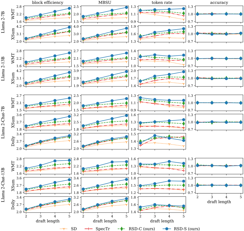
### Visual Description
## Chart: Performance Metrics vs. Draft Length for Language Models
### Overview
This image presents a series of four charts, arranged in a 2x2 grid, comparing the performance of several language models (Llama 2-7B, Llama 2-13B, Llama 2-70B, Dolly, and Spectr) across four metrics: block efficiency, MBSU (Memory Bandwidth per Second Utilization), token rate, and accuracy. The performance is evaluated as a function of "draft length," ranging from 1 to 5. Each chart displays multiple lines representing different algorithms or configurations (SD, Spectr, RSDC-ours, RSDS-ours).
### Components/Axes
* **X-axis (all charts):** Draft Length (ranging from 1 to 5, with tick marks at each integer value).
* **Y-axis (varies by chart):**
* Block Efficiency: Scale ranges from approximately 1.5 to 2.8.
* MBSU: Scale ranges from approximately 1.4 to 4.2.
* Token Rate: Scale ranges from approximately 0.8 to 1.4.
* Accuracy: Scale ranges from approximately 0.6 to 1.3.
* **Legend (bottom-center):**
* SD (Solid Dark Red Line)
* Spectr (Dashed Dark Red Line)
* RSDC-(ours) (Solid Teal Line)
* RSDS-(ours) (Dashed Teal Line)
* **Rows (top to bottom):**
* Llama 2-7B
* Llama 2-13B
* Llama 2-70B
* Dolly
* Llama 2-Chat-13B
* **Columns (left to right):**
* Block Efficiency
* MBSU
* Token Rate
* Accuracy
### Detailed Analysis or Content Details
**Llama 2-7B:**
* **Block Efficiency:** RSDC-(ours) shows a slight upward trend, starting at approximately 1.8 and reaching around 2.2. RSDS-(ours) is relatively flat around 1.6. SD starts at ~1.7 and ends at ~2.0. Spectr is flat around 1.6.
* **MBSU:** RSDC-(ours) increases from ~1.3 to ~1.9. RSDS-(ours) is relatively flat around 1.5. SD starts at ~2.0 and ends at ~3.0. Spectr is flat around 1.5.
* **Token Rate:** RSDC-(ours) increases from ~0.9 to ~1.3. RSDS-(ours) is relatively flat around 1.1. SD starts at ~0.7 and ends at ~1.1. Spectr is flat around 0.9.
* **Accuracy:** RSDC-(ours) is relatively flat around 1.0. RSDS-(ours) is relatively flat around 0.7. SD starts at ~0.7 and ends at ~1.0. Spectr is flat around 0.7.
**Llama 2-13B:**
* **Block Efficiency:** RSDC-(ours) shows a slight upward trend, starting at approximately 2.0 and reaching around 2.4. RSDS-(ours) is relatively flat around 1.8. SD starts at ~1.8 and ends at ~2.2. Spectr is flat around 1.6.
* **MBSU:** RSDC-(ours) increases from ~1.4 to ~2.0. RSDS-(ours) is relatively flat around 1.6. SD starts at ~2.0 and ends at ~3.9. Spectr is flat around 1.9.
* **Token Rate:** RSDC-(ours) increases from ~1.1 to ~1.4. RSDS-(ours) is relatively flat around 1.2. SD starts at ~0.9 and ends at ~1.4. Spectr is flat around 1.1.
* **Accuracy:** RSDC-(ours) is relatively flat around 1.1. RSDS-(ours) is relatively flat around 0.8. SD starts at ~0.7 and ends at ~1.3. Spectr is flat around 0.7.
**Llama 2-70B:**
* **Block Efficiency:** RSDC-(ours) shows a slight upward trend, starting at approximately 2.1 and reaching around 2.5. RSDS-(ours) is relatively flat around 1.9. SD starts at ~1.8 and ends at ~2.3. Spectr is flat around 1.8.
* **MBSU:** RSDC-(ours) increases from ~1.1 to ~1.9. RSDS-(ours) is relatively flat around 1.4. SD starts at ~1.9 and ends at ~3.0. Spectr is flat around 1.5.
* **Token Rate:** RSDC-(ours) increases from ~0.9 to ~1.3. RSDS-(ours) is relatively flat around 1.1. SD starts at ~0.7 and ends at ~1.1. Spectr is flat around 0.9.
* **Accuracy:** RSDC-(ours) is relatively flat around 1.0. RSDS-(ours) is relatively flat around 0.7. SD starts at ~0.7 and ends at ~1.0. Spectr is flat around 0.7.
**Dolly:**
* **Block Efficiency:** RSDC-(ours) shows a slight upward trend, starting at approximately 2.2 and reaching around 2.6. RSDS-(ours) is relatively flat around 2.0. SD starts at ~2.0 and ends at ~2.4. Spectr is flat around 1.8.
* **MBSU:** RSDC-(ours) increases from ~1.3 to ~2.6. RSDS-(ours) is relatively flat around 1.8. SD starts at ~1.8 and ends at ~3.2. Spectr is flat around 1.8.
* **Token Rate:** RSDC-(ours) increases from ~1.0 to ~1.4. RSDS-(ours) is relatively flat around 1.2. SD starts at ~0.8 and ends at ~1.2. Spectr is flat around 1.0.
* **Accuracy:** RSDC-(ours) is relatively flat around 1.1. RSDS-(ours) is relatively flat around 0.8. SD starts at ~0.7 and ends at ~1.1. Spectr is flat around 0.7.
**Llama 2-Chat-13B:**
* **Block Efficiency:** RSDC-(ours) shows a slight upward trend, starting at approximately 2.0 and reaching around 2.4. RSDS-(ours) is relatively flat around 1.8. SD starts at ~1.8 and ends at ~2.2. Spectr is flat around 1.6.
* **MBSU:** RSDC-(ours) increases from ~1.2 to ~2.4. RSDS-(ours) is relatively flat around 1.6. SD starts at ~1.8 and ends at ~3.6. Spectr is flat around 1.9.
* **Token Rate:** RSDC-(ours) increases from ~0.9 to ~1.3. RSDS-(ours) is relatively flat around 1.1. SD starts at ~0.7 and ends at ~1.1. Spectr is flat around 0.9.
* **Accuracy:** RSDC-(ours) is relatively flat around 0.9. RSDS-(ours) is relatively flat around 0.7. SD starts at ~0.7 and ends at ~1.0. Spectr is flat around 0.7.
### Key Observations
* SD consistently exhibits higher MBSU values across all models and draft lengths.
* RSDC-(ours) generally shows an increasing trend for Block Efficiency, MBSU, and Token Rate as draft length increases.
* RSDS-(ours) tends to be relatively stable across different draft lengths for all metrics.
* Spectr consistently shows the lowest performance across all metrics.
* Accuracy is generally lower for RSDS-(ours) compared to other algorithms.
### Interpretation
The data suggests that the RSDC-(ours) algorithm demonstrates improved performance with increasing draft length, particularly in terms of block efficiency, memory bandwidth utilization, and token rate. The SD algorithm consistently provides the highest MBSU, indicating efficient memory usage. The RSDS-(ours) algorithm maintains stable performance but generally lags behind RSDC-(ours) and SD. Spectr consistently underperforms, suggesting it may not be well-suited for these tasks or requires further optimization.
The consistent upward trend of RSDC-(ours) suggests that it benefits from longer draft lengths, potentially due to increased opportunities for optimization or better utilization of available resources. The stability of RSDS-(ours) might indicate a different optimization strategy that prioritizes consistency over maximizing performance with increasing draft length. The differences in accuracy suggest that the algorithms employ different strategies for generating accurate outputs, with SD and RSDC-(ours) generally achieving higher accuracy than RSDS-(ours) and Spectr. The data highlights the trade-offs between different algorithms in terms of performance, efficiency, and accuracy, and suggests that the optimal choice of algorithm depends on the specific application and requirements.
</details>
Figure 7. Block efficiency, MBSU, token rate and accuracy for varying lengths of draft sequence are given for multiple pairs of draft and target models: the size of draft model is in { 125M, 350M } , and the size of target model is in { 13B, 30B, 66B } . All results are normalized w.r.t. the values of AR decoding.
<details>
<summary>Image 7 Details</summary>
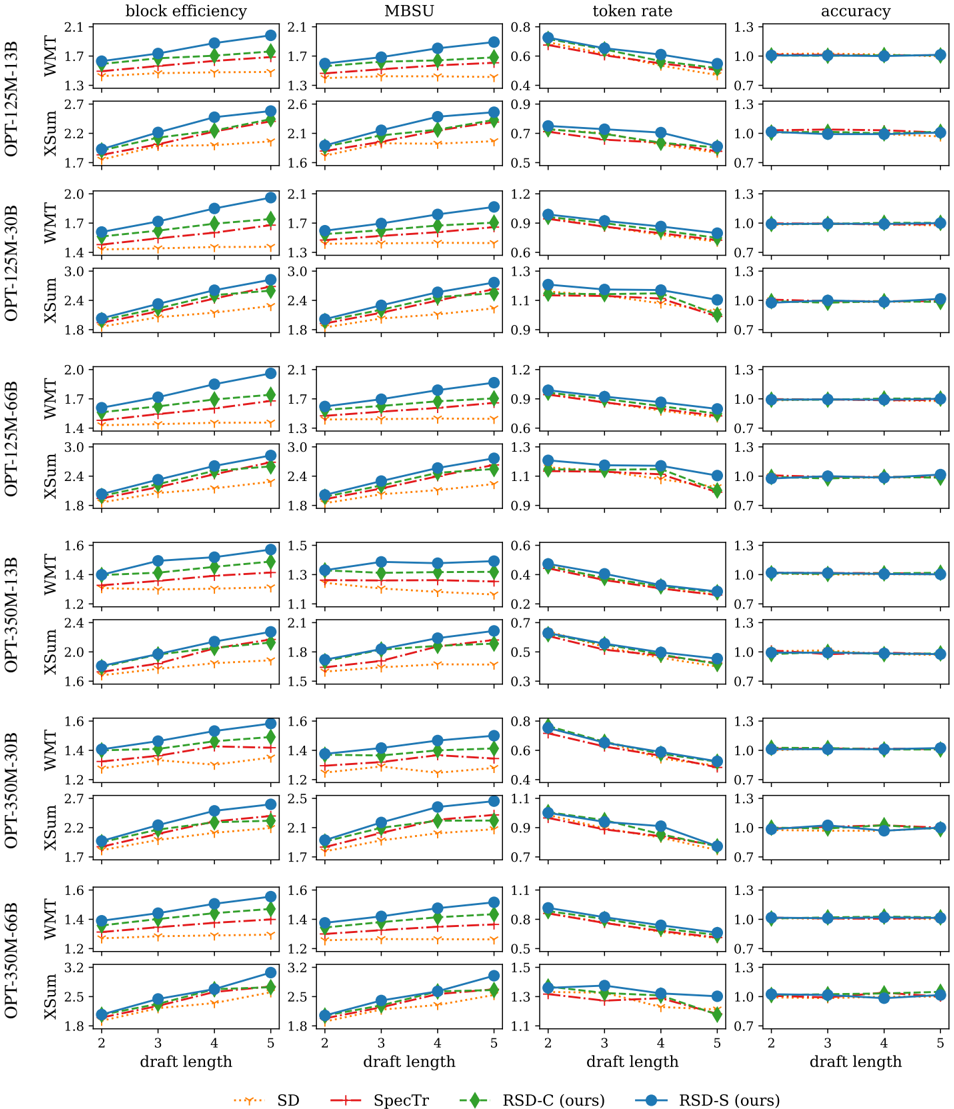
### Visual Description
\n
## Line Chart Grid: Performance Metrics vs. Draft Length
### Overview
The image presents a grid of line charts, comparing the performance of different model configurations (OPT-125M-3B, OPT-125M-6B, OPT-125M-30B, OPT-350M-1B, OPT-350M-30B, OPT-350M-6B) across four metrics: Block Efficiency, MBSU (Million Bytes Sent per Update), Token Rate, and Accuracy. Each row represents a different model, and each column represents a different metric. The x-axis in all charts represents "draft length" with values ranging from approximately 1 to 2.7.
### Components/Axes
* **X-axis (Common to all charts):** Draft Length (ranging from approximately 1.0 to 2.7, with markers at 1.2, 1.4, 1.6, 1.8, 2.0, 2.2, 2.4, 2.6
</details>
## C.4.2. BLOCK EFFICIENCY, MBSU, TOKEN RATE AND ACCURACY FOR VARIOUS TARGET COMPUTATIONAL BUDGET
Figure 8. Block efficiency, MBSU, token rate and accuracy for varying numbers of tokens processed at the target model are given for multiple target models: Llama 2-7B, Llama 2-13B, Llama 2-Chat-7B, Llama 2-Chat-13B. Chat models use the same draft model, while the other models use the same draft model different from the one for chat models. All results are normalized w.r.t. the values of AR decoding.
<details>
<summary>Image 8 Details</summary>
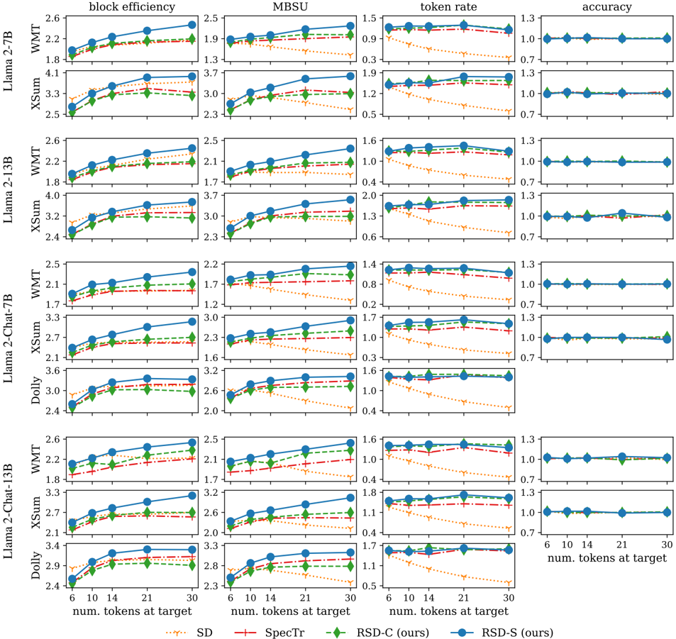
### Visual Description
\n
## Chart: Performance Metrics of Language Models
### Overview
The image presents a 5x4 grid of line charts comparing the performance of several language models (Llama 2-TB, Llama 2-13B, Llama 2-Chat-7B, Dolly, and Llama 2-Chat-13B) across four different metrics: block efficiency, MBSU (Memory Bandwidth per Second Utilization), token rate, and accuracy. Each chart displays performance as a function of the number of tokens at the target sequence length. Different lines within each chart represent different implementations: WMT (likely a specific training dataset or method) and XSum (another dataset/method). A third line, labeled "RSD-S (ours)", is also present in each chart.
### Components/Axes
* **X-axis (all charts):** "num. tokens at target" with values ranging from 2 to 30, with markers at 2, 6, 10, 14, 21, and 30.
* **Y-axis (varies by chart):**
* **Block Efficiency:** Scale from approximately 1.6 to 4.2.
* **MBSU:** Scale from approximately 1.2 to 3.7.
* **Token Rate:** Scale from approximately 0.2 to 1.6.
* **Accuracy:** Scale from approximately 0.6 to 1.3.
* **Legend (top-right, common to all charts):**
* WMT (Green line)
* XSum (Teal line)
* RSD-S (ours) (Red dashed line)
* **Title (above each chart):** Indicates the metric being displayed (block efficiency, MBSU, token rate, accuracy).
* **Row Labels (left side):** Indicate the language model being evaluated (Llama 2-TB, Llama 2-13B, Llama 2-Chat-7B, Dolly, Llama 2-Chat-13B).
* **Subtitle (bottom of the chart):** "Spectr" and "RSD-S (ours)"
### Detailed Analysis or Content Details
**Llama 2-TB:**
* **Block Efficiency:** XSum shows a generally increasing trend, starting at ~1.8 and reaching ~2.5 at 30 tokens. WMT is relatively flat around ~1.8. RSD-S starts at ~4.1 and decreases to ~3.3.
* **MBSU:** XSum increases from ~1.3 to ~2.3. WMT is relatively flat around ~1.9. RSD-S starts at ~3.7 and decreases to ~3.0.
* **Token Rate:** XSum increases from ~0.3 to ~0.9. WMT is relatively flat around ~0.5. RSD-S starts at ~1.2 and decreases to ~0.9.
* **Accuracy:** XSum is relatively flat around ~0.7. WMT is relatively flat around ~1.0. RSD-S is relatively flat around ~1.3.
**Llama 2-13B:**
* **Block Efficiency:** XSum increases from ~1.8 to ~3.2. WMT is relatively flat around ~2.4. RSD-S starts at ~4.0 and decreases to ~3.7.
* **MBSU:** XSum increases from ~2.1 to ~3.0. WMT is relatively flat around ~2.0. RSD-S starts at ~3.7 and decreases to ~3.0.
* **Token Rate:** XSum increases from ~0.6 to ~1.3. WMT is relatively flat around ~1.3. RSD-S starts at ~1.2 and decreases to ~0.9.
* **Accuracy:** XSum is relatively flat around ~0.7. WMT is relatively flat around ~1.3. RSD-S is relatively flat around ~1.3.
**Llama 2-Chat-7B:**
* **Block Efficiency:** XSum increases from ~1.7 to ~3.0. WMT is relatively flat around ~2.4. RSD-S starts at ~3.6 and decreases to ~3.2.
* **MBSU:** XSum increases from ~1.6 to ~2.6. WMT is relatively flat around ~2.2. RSD-S starts at ~3.2 and decreases to ~2.8.
* **Token Rate:** XSum increases from ~0.2 to ~0.8. WMT is relatively flat around ~0.8. RSD-S starts at ~1.0 and decreases to ~0.6.
* **Accuracy:** XSum is relatively flat around ~0.7. WMT is relatively flat around ~1.0. RSD-S is relatively flat around ~1.3.
**Dolly:**
* **Block Efficiency:** XSum increases from ~2.1 to ~3.6. WMT is relatively flat around ~2.4. RSD-S starts at ~3.0 and decreases to ~2.6.
* **MBSU:** XSum increases from ~1.7 to ~3.2. WMT is relatively flat around ~2.2. RSD-S starts at ~2.6 and decreases to ~2.0.
* **Token Rate:** XSum increases from ~0.4 to ~1.6. WMT is relatively flat around ~0.6. RSD-S starts at ~1.6 and decreases to ~1.0.
* **Accuracy:** XSum is relatively flat around ~0.7. WMT is relatively flat around ~0.7. RSD-S is relatively flat around ~1.3.
**Llama 2-Chat-13B:**
* **Block Efficiency:** XSum increases from ~2.1 to ~3.4. WMT is relatively flat around ~2.4. RSD-S starts at ~4.1 and decreases to ~3.8.
* **MBSU:** XSum increases from ~2.0 to ~3.2. WMT is relatively flat around ~2.4. RSD-S starts at ~3.8 and decreases to ~3.2.
* **Token Rate:** XSum increases from ~0.6 to ~1.4. WMT is relatively flat around ~1.4. RSD-S starts at ~1.4 and decreases to ~0.8.
* **Accuracy:** XSum is relatively flat around ~0.7. WMT is relatively flat around ~0.7. RSD-S is relatively flat around ~1.3.
### Key Observations
* RSD-S consistently outperforms WMT and XSum in all metrics, but often shows a decreasing trend as the number of tokens increases.
* XSum generally shows an increasing trend across all metrics, suggesting improved performance with longer sequences.
* WMT tends to be relatively stable across different sequence lengths.
* Dolly consistently has lower block efficiency, MBSU, and token rate compared to the Llama 2 models.
* Accuracy is generally higher for RSD-S and WMT compared to XSum.
### Interpretation
The charts demonstrate a comparative performance analysis of different language models and implementation strategies (WMT, XSum, RSD-S). The "RSD-S (ours)" implementation consistently achieves higher performance across all metrics, particularly in accuracy, but exhibits a diminishing return as the sequence length increases. This suggests that RSD-S may be more sensitive to longer sequences or may have limitations in scaling. The increasing trend observed in XSum indicates that its performance improves with longer sequences, potentially due to better utilization of context. The relatively stable performance of WMT suggests it is less sensitive to sequence length. The lower performance of Dolly compared to the Llama 2 models highlights the impact of model size and architecture on performance. The data suggests that the choice of implementation strategy (RSD-S, WMT, XSum) and model architecture (Llama 2 vs. Dolly) are crucial factors in optimizing language model performance. The decreasing trend of RSD-S could be due to memory constraints or computational bottlenecks as the sequence length increases. Further investigation is needed to understand the underlying reasons for these trends and to identify strategies for mitigating the performance degradation observed with RSD-S at longer sequence lengths.
</details>
Figure 9. Block efficiency, MBSU, token rate and accuracy for varying numbers of tokens processed at the target model are given for multiple pairs of draft and target models: the size of draft model is in { 125M, 350M } , and the size of target model is in { 13B, 30B, 66B } . All results are normalized w.r.t. the values of AR decoding.
<details>
<summary>Image 9 Details</summary>
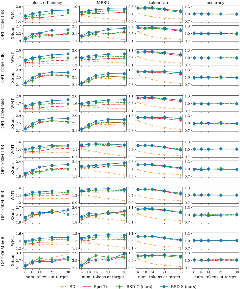
### Visual Description
\n
## Line Chart: Model Performance Metrics vs. Number of Layers
### Overview
The image presents a series of line charts comparing the performance of different language models (OPT-125M-1.3B, OPT-125M-3B, OPT-125M-6B, OPT-350M-1.3B, OPT-350M-30B, OPT-330M-60B) across four metrics: Block Efficiency, MBSU (Memory Bandwidth per Second Utilization), Token Rate, and Accuracy. The x-axis represents the number of layers (16, 32, 48, 64, 80, 96), and the y-axis scales vary for each metric. Each model is represented by three lines corresponding to different summation techniques: WMT, XSum, and XSum.
### Components/Axes
* **X-axis:** Number of Layers (16, 32, 48, 64, 80, 96)
* **Y-axes:**
* Block Efficiency: 1.2 to 2.0
* MBSU: 0.8 to 2.9
* Token Rate: 0.0 to 1.3
* Accuracy: 0.6 to 1.3
* **Models (Rows):**
* OPT-125M-1.3B
* OPT-125M-3B
* OPT-125M-6B
* OPT-350M-1.3B
* OPT-350M-30B
* OPT-330M-60B
* **Summation Techniques (Lines within each model):**
* WMT (Solid Line) - Color: Red
* XSum (Dashed Line) - Color: Green
* XSum (Dotted Line) - Color: Blue
* **Legend:** Located in the top-right corner, mapping colors to metrics.
### Detailed Analysis or Content Details
Here's a breakdown of the trends and approximate values for each metric and model. Note that values are estimated from the chart.
**OPT-125M-1.3B:**
* **Block Efficiency:** All three lines start around 1.4 and generally increase to around 1.7-1.8 by 96 layers. WMT shows a slight increase, XSum (dashed) is relatively flat, and XSum (dotted) shows a moderate increase.
* **MBSU:** Starts around 1.1 for all lines. WMT increases to ~1.5, XSum (dashed) to ~1.2, and XSum (dotted) to ~2.1 by 96 layers.
* **Token Rate:** Starts around 0.4 for all lines. WMT remains relatively flat around 0.4-0.5, XSum (dashed) increases to ~0.6, and XSum (dotted) increases to ~0.9 by 96 layers.
* **Accuracy:** All lines start around 0.7. WMT remains around 0.7, XSum (dashed) increases to ~0.8, and XSum (dotted) increases to ~1.0 by 96 layers.
**OPT-125M-3B:**
* **Block Efficiency:** Similar to 1.3B, lines start around 1.6 and increase to 1.7-1.9.
* **MBSU:** Starts around 1.2. WMT increases to ~1.9, XSum (dashed) to ~1.4, and XSum (dotted) to ~2.5 by 96 layers.
* **Token Rate:** Starts around 0.4. WMT remains flat, XSum (dashed) increases to ~0.6, and XSum (dotted) increases to ~1.1 by 96 layers.
* **Accuracy:** All lines start around 0.7. WMT remains around 0.7, XSum (dashed) increases to ~0.8, and XSum (dotted) increases to ~1.1 by 96 layers.
**OPT-125M-6B:**
* **Block Efficiency:** Starts around 1.4 and increases to 1.7-1.9.
* **MBSU:** Starts around 1.1. WMT increases to ~2.1, XSum (dashed) to ~1.6, and XSum (dotted) to ~2.5 by 96 layers.
* **Token Rate:** Starts around 0.4. WMT remains flat, XSum (dashed) increases to ~0.6, and XSum (dotted) increases to ~0.9 by 96 layers.
* **Accuracy:** All lines start around 0.7. WMT remains around 0.7, XSum (dashed) increases to ~0.8, and XSum (dotted) increases to ~1.1 by 96 layers.
**OPT-350M-1.3B:**
* **Block Efficiency:** Starts around 1.2 and increases to 1.4-1.6.
* **MBSU:** Starts around 0.9. WMT increases to ~1.7, XSum (dashed) to ~1.2, and XSum (dotted) to ~2.1 by 96 layers.
* **Token Rate:** Starts around 0.3. WMT remains flat, XSum (dashed) increases to ~0.6, and XSum (dotted) increases to ~1.0 by 96 layers.
* **Accuracy:** All lines start around 0.7. WMT remains around 0.7, XSum (dashed) increases to ~0.8, and XSum (dotted) increases to ~1.1 by 96 layers.
**OPT-350M-30B:**
* **Block Efficiency:** Starts around 1.2 and increases to 1.4-1.6.
* **MBSU:** Starts around 0.9. WMT increases to ~1.7, XSum (dashed) to ~1.2, and XSum (dotted) to ~2.1 by 96 layers.
* **Token Rate:** Starts around 0.3. WMT remains flat, XSum (dashed) increases to ~0.6, and XSum (dotted) increases to ~1.0 by 96 layers.
* **Accuracy:** All lines start around 0.7. WMT remains around 0.7, XSum (dashed) increases to ~0.8, and XSum (dotted) increases to ~1.1 by 96 layers.
**OPT-330M-60B:**
* **Block Efficiency:** Starts around 1.3 and increases to 1.5-1.7.
* **MBSU:** Starts around 1.0. WMT increases to ~1.9, XSum (dashed) to ~1.4, and XSum (dotted) to ~2.3 by 96 layers.
* **Token Rate:** Starts around 0.3. WMT remains flat, XSum (dashed) increases to ~0.6, and XSum (dotted) increases to ~1.0 by 96 layers.
* **Accuracy:** All lines start around 0.7. WMT remains around 0.7, XSum (dashed) increases to ~0.8, and XSum (dotted) increases to ~1.1 by 96 layers.
### Key Observations
* Generally, increasing the number of layers improves MBSU, Token Rate, and Accuracy, but the improvement plateaus after 64-80 layers for most models.
* The XSum (dotted) summation technique consistently outperforms WMT and XSum (dashed) across all metrics.
* Larger models (OPT-330M-60B) generally exhibit higher MBSU and Accuracy compared to smaller models (OPT-125M-1.3B).
* Block Efficiency shows relatively small changes across different models and summation techniques.
* WMT summation technique shows the least improvement with increasing layers.
### Interpretation
The data suggests that increasing model size and the number of layers generally improves performance, particularly in terms of memory bandwidth utilization (MBSU), token rate, and accuracy. The XSum (dotted) summation technique appears to be the most effective at leveraging increased model capacity. The plateauing of performance after a certain number of layers indicates diminishing returns, suggesting that further increasing model size beyond a certain point may not yield significant improvements. The consistent underperformance of the WMT summation technique suggests it may be less efficient at utilizing the available computational resources. This data is valuable for optimizing model architecture and training strategies to achieve the best possible performance for a given computational budget. The consistent trend across all models suggests a general principle about scaling language models, but further investigation is needed to understand the specific reasons behind these observations.
</details>
## C.5. Experient results with tables
For readers curious about raw numbers, we remain all the numbers used for plots as tables in this section.
C.5.1. BLOCK EFFICIENCY, MBSU, TOKEN RATE AND ACCURACY FOR VARYING LENGTHS OF DRAFT SEQUENCE
- Llama 2-7B (with 115M drafter)
- -XSum ( Table 1), WMT ( Table 2) · Llama 2-13B (with 115M drafter) -XSum ( Table 3), WMT ( Table 4) · Llama 2-70B (with 115M drafter) -XSum ( Table 5), WMT ( Table 6) · Llama 2-Chat-7B (with 115M drafter) -XSum ( Table 7), WMT ( Table 8), Dolly ( Table 9) · Llama 2-Chat-13B (with 115M drafter) -XSum ( Table 10), WMT ( Table 11), Dolly ( Table 12) · Llama 2-Chat-70B (with 115M drafter) -XSum ( Table 13), WMT ( Table 14), Dolly ( Table 15) · OPT-13B (with OPT-125M drafter) -XSum ( Table 16), WMT ( Table 17) · OPT-30B (with OPT-125M drafter) -XSum ( Table 18), WMT ( Table 19) · OPT-66B (with OPT-125M drafter) -XSum ( Table 20), WMT ( Table 21) · OPT-13B (with OPT-350M drafter) -XSum ( Table 22), WMT ( Table 23) · OPT-30B (with OPT-350M drafter) -XSum ( Table 24), WMT ( Table 25) · OPT-66B (with OPT-350M drafter) -XSum ( Table 26), WMT ( Table 27)
- C.5.2. BLOCK EFFICIENCY, MBSU, TOKEN RATE AND ACCURACY FOR VARYING NUMBERS OF TOKENS PROCESSED AT THE TARGET MODEL
- Llama 2-7B (with 115M drafter) -XSum ( Table 28), WMT ( Table 29) · Llama 2-13B (with 115M drafter) -XSum ( Table 30), WMT ( Table 31) · Llama 2-70B (with 115M drafter) -XSum ( Table 32), WMT ( Table 33) · Llama 2-Chat-7B (with 115M drafter) -XSum ( Table 34), WMT ( Table 35), Dolly ( Table 36) · Llama 2-Chat-13B (with 115M drafter) -XSum ( Table 37), WMT ( Table 38), Dolly ( Table 39) · Llama 2-Chat-70B (with 115M drafter) -XSum ( Table 40), WMT ( Table 41), Dolly ( Table 42) · OPT-13B (with OPT-125M drafter) -XSum ( Table 43), WMT ( Table 44) · OPT-30B (with OPT-125M drafter) -XSum ( Table 45), WMT ( Table 46) · OPT-66B (with OPT-125M drafter) -XSum ( Table 47), WMT ( Table 48) · OPT-13B (with OPT-350M drafter) -XSum ( Table 49), WMT ( Table 50) · OPT-30B (with OPT-350M drafter) -XSum ( Table 51), WMT ( Table 52) · OPT-66B (with OPT-350M drafter) -XSum ( Table 53), WMT ( Table 54)
Table 1. We summarize experiment results with Llama 2-7B target and 115M draft for the XSum task with various draft lengths. Draft Length (DL) means the (maximum) length for all draft token sequences generated by the draft model. For decoders (Dec.), we consider Auto-Regressive sampling (AR), Speculative Decoding (SD), SpecTr, Recursive Speculative Decoding with Constant branching factors (RSD-C), Recursive Speculative Decoding with Stochastic Beam Search (RSD-S). The contents in decoder specification (Spec.) have different meanings for each decoder; K × L means the number K of draft paths and draft length L for SpecTr; it describes constant branching factors for each level of the tree (from root to leaf) for RSD-C; K × L means the beamwidth K and draft length L for RSD-S. Block efficiency (Eff.), Memory Bound Speed Up (MBSU), Token Rate (TR), and Accuracy (Acc.) are given for each algorithm. For each group of rows having the same complexity, we highlight the best values for all columns except accuracy.
| Model | Task | DL | Dec. | Spec. | Eff. | MBSU | TR | Acc. |
|---------|--------|------|--------|--------------------|-------------|-------------|--------|--------|
| | | 0 | AR | - | 1.000 | 1.000 | 37.269 | 0.141 |
| | | 0 | SD | 2 | 2.166 | 2.093 | 51.515 | 0.143 |
| | | 0 | | 2 × 2 | 2.218 | 2.143 | 52.95 | 0.146 |
| | | 0 | SpecTr | 3 × 2 | 2.279 | 2.202 | 53.346 | 0.139 |
| | | 2 | | 2 - 1 | 2.267 | 2.191 | 53.98 | 0.142 |
| | | 0 | RSD-C | 2 - 2 | 2.398 | 2.317 | 56.609 | 0.143 |
| | | 0 | | 3 - 1 | 2.291 | 2.214 | 53.93 | 0.14 |
| | | 0 | | 2 × 2 | 2.367 | 2.288 | 54.586 | 0.143 |
| | | 0 | RSD-S | 3 × 2 | 2.432 | 2.350 | 55.465 | 0.14 |
| | | 3 | SD | 3 | 2.465 | 2.343 | 54.195 | 0.14 |
| | | | SpecTr | 3 × 3 | 2.644 | 2.513 | 55.273 | 0.14 |
| | | | | 4 × 3 | 2.718 | 2.583 | 56.688 | 0.145 |
| | | | | 2 - 2 - 2 | 2.868 | 2.726 | 59.879 | 0.141 |
| | | | RSD-C | 3 - 1 - 1 | 2.641 | 2.511 | 55.384 | 0.143 |
| | | | | 4 - 1 - 1 | 2.688 | 2.555 | 57.518 | 0.14 |
| | | | | 3 × 3 | 2.927 | 2.782 | 58.843 | 0.139 |
| Llama | XSum | | RSD-S | 4 × 3 | 2.970 | 2.823 | 61.937 | 0.136 |
| | | | SD | 4 | 2.728 | 2.551 | 53.731 | 0.137 |
| | | | | 5 × 4 | 2.974 | 2.781 | 56.002 | 0.144 |
| | | | SpecTr | 7 × 4 | 3.093 | 2.892 | 60.053 | 0.139 |
| | | 4 | | 2 - 2 - 2 - 2 | 3.205 | 2.997 | 61.723 | 0.142 |
| | | | RSD-C | 5 - 1 - 1 - 1 | 2.898 | 2.710 | 56.343 | 0.141 |
| | | | | 7 - 1 - 1 - 1 | 2.974 | 2.781 | 58.423 | 0.137 |
| | | | | 5 × 4 | 3.427 | 3.205 | 64.887 | 0.14 |
| | | | RSD-S | 7 × 4 | 3.535 | 3.306 | 64.456 | 0.14 |
| | | | SD | 5 | 2.865 | 2.636 | 53.199 | 0.14 |
| | | | | 6 × 5 | 3.209 | 2.953 | 55.424 | 0.141 |
| | | | SpecTr | 12 × 5 | 3.425 | 3.152 | 60.133 | 0.141 |
| | | 5 | | 2 - 2 - 2 - 2 - 2 | 3.492 | 3.213 | 62.753 | 0.143 |
| | | | RSD-C | 6 - 1 - 1 - 1 - 1 | 3.133 | 2.883 | 55.796 | 0.142 |
| | | | | 1 - 1 | | | 58.352 | 0.141 |
| | | | RSD-S | 12 - 1 - 1 - 6 × 5 | 3.249 3.811 | 2.990 3.507 | 65.16 | 0.141 |
Table 2. We summarize experiment results with Llama 2-7B target and 115M draft for the WMT task with various draft lengths. Draft Length (DL) means the (maximum) length for all draft token sequences generated by the draft model. For decoders (Dec.), we consider Auto-Regressive sampling (AR), Speculative Decoding (SD), SpecTr, Recursive Speculative Decoding with Constant branching factors (RSD-C), Recursive Speculative Decoding with Stochastic Beam Search (RSD-S). The contents in decoder specification (Spec.) have different meanings for each decoder; K × L means the number K of draft paths and draft length L for SpecTr; it describes constant branching factors for each level of the tree (from root to leaf) for RSD-C; K × L means the beamwidth K and draft length L for RSD-S. Block efficiency (Eff.), Memory Bound Speed Up (MBSU), Token Rate (TR), and Accuracy (Acc.) are given for each algorithm. For each group of rows having the same complexity, we highlight the best values for all columns except accuracy.
| Model | Task | DL | Dec. | Spec. | Eff. | MBSU | TR | Acc. |
|---------|--------|------|--------|----------------------|-------------|-------------|---------------|-------------|
| | | 0 | AR | - | 1.000 | 1.000 | 37.631 | 0.374 |
| | | | SD | 2 | 1.673 | 1.617 | 42.447 | 0.370 |
| | | | | 2 × 2 | 1.727 | 1.669 | 42.013 | 0.370 |
| | | | SpecTr | 3 × 2 | 1.757 | 1.698 | 43.128 | 0.376 |
| | | | | 2 - 1 | 1.768 | 1.708 | 43.044 | 0.377 |
| | | 2 | RSD-C | 2 - 2 | 1.858 | 1.796 | 45.245 | 0.372 |
| | | | | 3 - 1 | 1.819 | 1.758 | 44.482 | 0.375 |
| | | | RSD-S | 2 × 2 | 1.824 | 1.763 | 43.536 | 0.370 |
| | | | | 3 × 2 | 1.912 | 1.847 | 45.018 | 0.373 |
| | | | SD | 3 | 1.783 | 1.695 | 40.816 | 0.374 |
| | | | | 3 × 3 | 1.890 | 1.796 | 42.746 | 0.381 |
| | | | SpecTr | 4 × 3 | 1.913 | 1.819 | 41.990 | 0.379 |
| | | | | 2 - 2 - 2 | 2.033 | 1.933 | 44.669 | 0.372 |
| | | 3 | RSD-C | 3 - 1 - 1 | 1.940 | 1.844 | 42.981 | 0.370 |
| | | | | 4 - 1 - 1 | 1.981 | 1.883 | 43.791 | 0.376 |
| | | | | 3 × 3 | 2.064 | 1.962 | 43.684 | 0.372 |
| Llama | WMT | | RSD-S | 4 × 3 | 2.143 | 2.037 | 45.766 | 0.374 |
| | | | SD | 4 | 1.854 | 1.734 | 38.651 | 0.377 |
| | | | | 5 × 4 | 2.023 | 1.892 | 41.134 | 0.375 |
| | | | SpecTr | 7 × 4 | 2.059 | 1.925 | 42.573 | 0.373 |
| | | | | 2 - 2 - 2 - 2 | 2.152 | 2.013 | 43.755 | 0.378 |
| | | 4 | RSD-C | 5 - 1 - 1 - 1 | 2.083 | 1.948 | 43.142 | 0.375 |
| | | | | 7 - 1 - 1 - 1 | 2.130 | 1.992 | 42.567 | 0.375 |
| | | | | 5 × 4 | 2.311 | 2.161 | 44.367 | 0.375 |
| | | | RSD-S | 7 × 4 | 2.408 | 2.252 | 46.197 | 0.376 |
| | | | SD | 5 | 1.910 | 1.758 | 36.041 | 0.378 |
| | | | SpecTr | 6 × 5 | 2.120 | 1.951 | 38.841 | 0.373 |
| | | | | 12 × 5 | 2.176 | 2.002 | 39.702 | 0.376 |
| | | | | 2 - 2 - 2 - 2 - 2 | 2.234 | 2.056 | 42.161 | 0.375 |
| | | 5 | RSD-C | 6 - 1 - 1 - 1 - | 2.171 | 1.998 | 40.331 | 0.372 |
| | | | | 1 12 - 1 - 1 - 1 - 1 | 2.249 | 2.070 | 41.585 | 0.376 |
| | | | RSD-S | 6 × 5 12 × 5 | 2.467 2.657 | 2.270 2.445 | 43.898 46.843 | 0.370 0.374 |
Table 3. We summarize experiment results with Llama 2-13B target and 115M draft for the XSum task with various draft lengths. Draft Length (DL) means the (maximum) length for all draft token sequences generated by the draft model. For decoders (Dec.), we consider Auto-Regressive sampling (AR), Speculative Decoding (SD), SpecTr, Recursive Speculative Decoding with Constant branching factors (RSD-C), Recursive Speculative Decoding with Stochastic Beam Search (RSD-S). The contents in decoder specification (Spec.) have different meanings for each decoder; K × L means the number K of draft paths and draft length L for SpecTr; it describes constant branching factors for each level of the tree (from root to leaf) for RSD-C; K × L means the beamwidth K and draft length L for RSD-S. Block efficiency (Eff.), Memory Bound Speed Up (MBSU), Token Rate (TR), and Accuracy (Acc.) are given for each algorithm. For each group of rows having the same complexity, we highlight the best values for all columns except accuracy.
| Model | Task | DL | Dec. | Spec. | Eff. | MBSU | TR | Acc. |
|---------|--------|------|--------|----------------------|-------------|-------------|---------------|-------------|
| | | 0 | AR | - | 1.000 | 1.000 | 28.141 | 0.166 |
| | | 0 | SD | 2 | 2.120 | 2.082 | 40.958 | 0.164 |
| | | 0 | | 2 × 2 | 2.172 | 2.133 | 40.870 | 0.170 |
| | | 0 | SpecTr | 3 × 2 | 2.212 | 2.173 | 41.116 | 0.165 |
| | | 2 | | 2 - 1 | 2.224 | 2.185 | 41.866 | 0.165 |
| | | 0 | RSD-C | 2 - 2 | 2.347 | 2.305 | 44.593 | 0.166 |
| | | 0 | | 3 - 1 | 2.269 | 2.229 | 42.981 | 0.158 |
| | | 0 | RSD-S | 2 × 2 | 2.311 | 2.271 | 43.533 | 0.165 |
| | | 0 | | 3 × 2 | 2.412 | 2.370 | 44.529 | 0.162 |
| | | 3 | SD | 3 | 2.377 | 2.315 | 42.777 | 0.160 |
| | | | | 3 × 3 | 2.559 | 2.492 | 45.252 | 0.166 |
| | | | SpecTr | 4 × 3 | 2.578 | 2.510 | 44.703 | 0.164 |
| | | | | 2 - 2 - 2 | 2.784 | 2.711 | 47.985 | 0.166 |
| | | | RSD-C | 3 - 1 - 1 | 2.560 | 2.493 | 44.855 | 0.164 |
| | | | | 4 - 1 - 1 | 2.593 | 2.525 | 44.639 | 0.161 |
| | | | | 3 × 3 | 2.832 | 2.758 | 48.388 | 0.162 |
| Llama | XSum | | RSD-S | 4 × 3 | 2.919 | 2.842 | 50.092 | 0.163 |
| | | | SD | 4 | 2.608 | 2.517 | 43.309 | 0.165 |
| | | | | 5 × 4 | 2.880 | 2.780 | 45.940 | 0.161 |
| | | | SpecTr | 7 × 4 | 2.944 | 2.842 | 47.456 | 0.162 |
| | | 4 | | 2 - 2 - 2 - 2 | 3.096 | 2.989 | 49.203 | 0.167 |
| | | | RSD-C | 5 - 1 - 1 - 1 | 2.813 | 2.715 | 44.641 | 0.165 |
| | | | | 7 - 1 - 1 - 1 | 2.864 | 2.764 | 45.288 | 0.162 |
| | | | | 5 × 4 | 3.347 | 3.231 | 50.517 | 0.163 |
| | | | RSD-S | 7 × 4 | 3.442 | 3.322 | 52.105 | 0.157 |
| | | | SD | 5 | 2.738 | 2.621 | 41.562 | 0.165 |
| | | | | 6 × 5 | 3.108 | 2.974 | 46.120 | 0.169 |
| | | | SpecTr | 12 × 5 | 3.230 | 3.091 | 46.587 | 0.166 |
| | | 5 | | 2 - 2 - 2 - 2 - 2 | 3.365 | 3.220 | 48.923 | 0.165 |
| | | | RSD-C | 6 - 1 - 1 - 1 - 1 | 3.014 | 2.885 | 43.751 | 0.163 |
| | | | RSD-S | 6 5 12 × 5 | 3.648 3.948 | 3.492 3.778 | 50.782 55.044 | 0.164 |
| | | | | 12 - 1 - 1 - 1 - 1 × | 3.069 | 2.937 | 44.262 | 0.164 0.162 |
Table 4. We summarize experiment results with Llama 2-13B target and 115M draft for the WMT task with various draft lengths. Draft Length (DL) means the (maximum) length for all draft token sequences generated by the draft model. For decoders (Dec.), we consider Auto-Regressive sampling (AR), Speculative Decoding (SD), SpecTr, Recursive Speculative Decoding with Constant branching factors (RSD-C), Recursive Speculative Decoding with Stochastic Beam Search (RSD-S). The contents in decoder specification (Spec.) have different meanings for each decoder; K × L means the number K of draft paths and draft length L for SpecTr; it describes constant branching factors for each level of the tree (from root to leaf) for RSD-C; K × L means the beamwidth K and draft length L for RSD-S. Block efficiency (Eff.), Memory Bound Speed Up (MBSU), Token Rate (TR), and Accuracy (Acc.) are given for each algorithm. For each group of rows having the same complexity, we highlight the best values for all columns except accuracy.
| Model | Task | DL | Dec. | Spec. | Eff. | MBSU | TR | Acc. |
|---------|--------|------|--------|---------------------|-------------|-------------|---------------|-------------|
| | | 0 | AR | - | 1.000 | 1.000 | 30.467 | 0.413 |
| | | | SD | 2 | 1.662 | 1.632 | 34.571 | 0.410 |
| | | | | 2 × 2 | 1.717 | 1.686 | 35.383 | 0.405 |
| | | | SpecTr | 3 × 2 | 1.748 | 1.717 | 35.124 | 0.408 |
| | | | | 2 - 1 | 1.760 | 1.729 | 36.200 | 0.405 |
| | | 2 | RSD-C | 2 - 2 | 1.852 | 1.819 | 38.384 | 0.407 |
| | | | | 3 - 1 | 1.815 | 1.783 | 37.576 | 0.408 |
| | | | RSD-S | 2 × 2 | 1.810 | 1.778 | 35.906 | 0.404 |
| | | | | 3 × 2 | 1.903 | 1.869 | 37.934 | 0.410 |
| | | | SD | 3 | 1.778 | 1.731 | 34.213 | 0.408 |
| | | | | 3 × 3 | 1.876 | 1.827 | 35.754 | 0.407 |
| | | | SpecTr | 4 × 3 | 1.903 | 1.853 | 35.127 | 0.409 |
| | | | | 2 - 2 - 2 | 2.027 | 1.974 | 36.916 | 0.407 |
| | | 3 | RSD-C | 3 - 1 - 1 | 1.929 | 1.878 | 37.279 | 0.413 |
| | | | | 4 - 1 - 1 | 1.965 | 1.914 | 35.558 | 0.408 |
| | | | | 3 × 3 | 2.059 | 2.005 | 36.511 | 0.406 |
| Llama | WMT | | RSD-S | 4 × 3 | 2.141 | 2.084 | 39.415 | 0.413 |
| | | | SD | 4 | 1.852 | 1.787 | 33.728 | 0.406 |
| | | | | 5 × 4 | 2.004 | 1.935 | 34.950 | 0.409 |
| | | | SpecTr | 7 × 4 | 2.038 | 1.968 | 34.973 | 0.411 |
| | | | | 2 - 2 - 2 - 2 | 2.122 | 2.048 | 36.819 | 0.407 |
| | | 4 | RSD-C | 5 - 1 - 1 - 1 | 2.080 | 2.008 | 35.434 | 0.411 |
| | | | | 7 - 1 - 1 - 1 | 2.116 | 2.042 | 35.526 | 0.406 |
| | | | | 5 × 4 | 2.304 | 2.224 | 37.842 | 0.408 |
| | | | RSD-S | 7 × 4 | 2.399 | 2.315 | 38.315 | 0.410 |
| | | | SD | 5 | 1.913 | 1.831 | 31.396 | 0.406 |
| | | | SpecTr | 12 × 5 | 2.101 | 2.011 | 34.184 | 0.408 |
| | | | | 6 × 5 | 2.168 | 2.074 | 34.936 | 0.408 |
| | | | | 2 - 2 - 2 - - 2 | 2.198 | 2.103 | 34.472 | 0.412 |
| | | 5 | RSD-C | 2 6 - 1 - 1 - 1 - 1 | 2.163 | 2.070 | 34.502 | 0.408 |
| | | | RSD-S | 6 × 5 12 × 5 | 2.448 2.638 | 2.343 2.525 | 35.575 39.182 | 0.410 0.412 |
| | | | | 12 - 1 - 1 - 1 - 1 | 2.238 | 2.142 | 36.278 | 0.408 |
Table 5. We summarize experiment results with Llama 2-70B target and 115M draft for the XSum task with various draft lengths. Draft Length (DL) means the (maximum) length for all draft token sequences generated by the draft model. For decoders (Dec.), we consider Auto-Regressive sampling (AR), Speculative Decoding (SD), SpecTr, Recursive Speculative Decoding with Constant branching factors (RSD-C), Recursive Speculative Decoding with Stochastic Beam Search (RSD-S). The contents in decoder specification (Spec.) have different meanings for each decoder; K × L means the number K of draft paths and draft length L for SpecTr; it describes constant branching factors for each level of the tree (from root to leaf) for RSD-C; K × L means the beamwidth K and draft length L for RSD-S. Block efficiency (Eff.), Memory Bound Speed Up (MBSU), Token Rate (TR), and Accuracy (Acc.) are given for each algorithm. For each group of rows having the same complexity, we highlight the best values for all columns except accuracy.
| Model | Task | DL | Dec. | Spec. | Eff. | MBSU | TR | Acc. |
|---------|--------|------|--------|--------------------|-------------|-------------|---------------|-------------|
| | | 0 | AR | - | 1.000 | 1.000 | 9.079 | 0.194 |
| | | 0 | SD | 2 | 2.103 | 2.096 | 15.054 | 0.188 |
| | | 0 | | 2 × 2 | 2.164 | 2.157 | 15.171 | 0.189 |
| | | 0 | SpecTr | 3 × 2 | 2.204 | 2.197 | 15.346 | 0.191 |
| | | 2 | | 2 - 1 | 2.189 | 2.181 | 15.276 | 0.187 |
| | | 0 | RSD-C | 2 - 2 | 2.322 | 2.314 | 16.033 | 0.189 |
| | | 0 | | 3 - 1 | 2.239 | 2.231 | 15.480 | 0.197 |
| | | 0 | RSD-S | 2 × 2 | 2.288 | 2.280 | 15.719 | 0.189 |
| | | 0 | | 3 × 2 | 2.376 | 2.368 | 16.284 | 0.193 |
| | | 3 | SD | 3 | 2.365 | 2.353 | 15.992 | 0.193 |
| | | | | 3 × 3 | 2.528 | 2.515 | 16.533 | 0.195 |
| | | | SpecTr | 4 × 3 | 2.554 | 2.541 | 16.586 | 0.193 |
| | | | | 2 - 2 - 2 | 2.757 | 2.743 | 17.790 | 0.188 |
| | | | RSD-C | 3 - 1 - 1 | 2.551 | 2.538 | 16.837 | 0.189 |
| | | | | 4 - 1 - 1 | 2.543 | 2.531 | 16.617 | 0.196 |
| | | | | 3 × 3 | 2.765 | 2.751 | 17.689 | 0.192 |
| Llama | XSum | | RSD-S | 4 × 3 | 2.862 | 2.848 | 18.163 | 0.186 |
| | | | SD | 4 | 2.584 | 2.566 | 16.656 | 0.196 |
| | | | | 5 × 4 | 2.844 | 2.825 | 17.159 | 0.192 |
| | | | SpecTr | 7 × 4 | 2.883 | 2.863 | 17.052 | 0.192 |
| | | 4 | | 2 - 2 - 2 - 2 | 3.028 | 3.008 | 17.885 | 0.191 |
| | | | RSD-C | 5 - 1 - 1 - 1 | 2.749 | 2.730 | 16.658 | 0.193 |
| | | | | 7 - 1 - 1 - 1 | 2.780 | 2.762 | 16.568 | 0.190 |
| | | | | 5 × 4 | 3.242 | 3.220 | 18.965 | 0.196 |
| | | | RSD-S | 7 × 4 | 3.361 | 3.338 | 19.248 | 0.191 |
| | | | SD | 5 | 2.680 | 2.658 | 16.634 | 0.194 |
| | | | | 6 × 5 | 3.103 | 3.077 | 17.603 | 0.192 |
| | | | SpecTr | 12 × 5 | 3.206 | 3.179 | 17.344 | 0.194 |
| | | 5 | | 2 - 2 - 2 - 2 - 2 | 3.295 | 3.268 | 17.675 | 0.191 |
| | | | RSD-C | 6 - 1 - 1 - 1 - 1 | 2.935 | 2.910 | 16.809 | 0.193 |
| | | | RSD-S | 6 × 5 12 × 5 | 3.556 3.851 | 3.526 3.819 | 16.371 19.808 | 0.194 |
| | | | | 12 - 1 - 1 - 1 - 1 | 3.004 | 2.978 | 19.484 | 0.193 0.192 |
Table 6. We summarize experiment results with Llama 2-70B target and 115M draft for the WMT task with various draft lengths. Draft Length (DL) means the (maximum) length for all draft token sequences generated by the draft model. For decoders (Dec.), we consider Auto-Regressive sampling (AR), Speculative Decoding (SD), SpecTr, Recursive Speculative Decoding with Constant branching factors (RSD-C), Recursive Speculative Decoding with Stochastic Beam Search (RSD-S). The contents in decoder specification (Spec.) have different meanings for each decoder; K × L means the number K of draft paths and draft length L for SpecTr; it describes constant branching factors for each level of the tree (from root to leaf) for RSD-C; K × L means the beamwidth K and draft length L for RSD-S. Block efficiency (Eff.), Memory Bound Speed Up (MBSU), Token Rate (TR), and Accuracy (Acc.) are given for each algorithm. For each group of rows having the same complexity, we highlight the best values for all columns except accuracy.
| Model | Task | DL | Dec. | Spec. | Eff. | MBSU | TR | Acc. |
|---------|--------|------|--------|-------------------------------|-------------------|-------------------|----------------------|-------------------|
| | | 0 | AR | - | 1.000 | 1.000 | 9.706 | 0.439 |
| | | | SD | 2 | 1.661 | 1.655 | 13.331 | 0.440 |
| | | | | 2 × 2 | 1.732 | 1.726 | 13.742 | 0.445 |
| | | | SpecTr | 3 × 2 | 1.756 | 1.750 | 13.710 | 0.445 |
| | | | | 2 - 1 | 1.770 | 1.764 | 13.992 | 0.436 |
| | | 2 | RSD-C | 2 - 2 | 1.853 | 1.847 | 14.512 | 0.443 |
| | | | | 3 - 1 | 1.819 | 1.813 | 14.245 | 0.440 |
| | | | RSD-S | 2 × 2 | 1.819 | 1.813 | 14.211 | 0.438 |
| | | | | 3 × 2 | 1.907 | 1.900 | 14.727 | 0.439 |
| | | | SD | 3 | 1.778 | 1.769 | 13.620 | 0.442 |
| | | | | 3 × 3 | 1.880 | 1.870 | 13.906 | 0.440 |
| | | | SpecTr | 4 × 3 | 1.909 | 1.899 | 13.959 | 0.437 |
| | | | | 2 - 2 - 2 | 2.021 | 2.010 | 14.875 | 0.438 |
| | | 3 | RSD-C | 3 - 1 - 1 | 1.940 | 1.930 | 14.474 | 0.441 |
| | | | | 4 - 1 - 1 | 1.968 | 1.958 | 14.483 | 0.439 |
| | | | | 3 × 3 | 2.068 | 2.057 | 15.132 | 0.440 |
| Llama | WMT | | RSD-S | 4 × 3 | 2.140 | 2.129 | 15.591 | 0.437 |
| | | | SD | 4 | 1.866 | 1.854 | 13.698 | 0.437 |
| | | | | 5 × 4 | 2.016 | 2.003 | 13.865 | 0.440 |
| | | | SpecTr | 7 × 4 | 2.048 | 2.034 | 13.833 | 0.441 |
| | | | | 2 - 2 - 2 - 2 | 2.130 | 2.116 | 14.338 | 0.440 |
| | | 4 | RSD-C | 5 - 1 - 1 - 1 | 2.088 | 2.074 | 14.311 | 0.440 |
| | | | | 7 - 1 - 1 - 1 | 2.132 | 2.117 | 14.406 | 0.441 |
| | | | | 5 × 4 | 2.309 | 2.293 | 15.550 | 0.434 |
| | | | RSD-S | 7 × 4 | 2.408 | 2.392 | 15.962 | 0.437 |
| | | | SD | 5 | 1.917 | 1.901 | 13.430 | 0.437 |
| | | | SpecTr | 12 × 5 | 2.113 | 2.095 | 13.737 | 0.443 |
| | | | | 6 × 5 | 2.177 | 2.159 | 13.619 | 0.442 |
| | | | | - - - - | 2.232 | 2.214 | 13.988 | 0.443 |
| | | 5 | RSD-C | 2 2 2 2 2 6 - 1 - 1 - 1 - 1 | 2.173 | | | |
| | | | | | | 2.154 | 14.095 | 0.440 |
| | | | RSD-S | 12 - 1 - 1 - 1 - 6 × 5 12 × 5 | 2.246 2.451 2.650 | 2.227 2.430 2.628 | 14.022 15.575 15.941 | 0.440 0.439 0.439 |
Table 7. We summarize experiment results with Llama 2-Chat-7B target and 115M draft for the XSum task with various draft lengths. Draft Length (DL) means the (maximum) length for all draft token sequences generated by the draft model. For decoders (Dec.), we consider Auto-Regressive sampling (AR), Speculative Decoding (SD), SpecTr, Recursive Speculative Decoding with Constant branching factors (RSD-C), Recursive Speculative Decoding with Stochastic Beam Search (RSD-S). The contents in decoder specification (Spec.) have different meanings for each decoder; K × L means the number K of draft paths and draft length L for SpecTr; it describes constant branching factors for each level of the tree (from root to leaf) for RSD-C; K × L means the beamwidth K and draft length L for RSD-S. Block efficiency (Eff.), Memory Bound Speed Up (MBSU), Token Rate (TR), and Accuracy (Acc.) are given for each algorithm. For each group of rows having the same complexity, we highlight the best values for all columns except accuracy.
| Model | Task | DL | Dec. | Spec. | Eff. | MBSU | TR | Acc. |
|---------|--------|------|--------|-------------------------|--------|--------|--------|-------------|
| | | 0 | AR | - | 1 | 1 | 41.651 | 0.092 |
| | | | SD | 2 | 1.938 | 1.873 | 47.708 | 0.091 |
| | | | | 2 × 2 | 1.961 | 1.896 | 46.422 | 0.092 |
| | | | SpecTr | 3 × 2 | 1.972 | 1.906 | 45.886 | 0.092 |
| | | 2 | | 2 - 1 | 2.048 | 1.979 | 49.725 | 0.091 |
| | | | RSD-C | 2 - 2 | 2.162 | 2.09 | 51.949 | 0.089 |
| | | | | 3 - 1 | 2.1 | 2.03 | 50.115 | 0.091 |
| | | | RSD-S | 2 × 2 | 2.129 | 2.058 | 50.315 | 0.090 |
| | | | | 3 × 2 | 2.22 | 2.146 | 52.867 | 0.090 |
| | | | SD | 3 | 2.144 | 2.038 | 47.36 | 0.090 |
| | | | SpecTr | 3 × 3 | 2.202 | 2.093 | 46.211 | 0.092 |
| | | | | 4 × 3 | 2.211 | 2.102 | 46.96 | 0.091 |
| | | 3 | | 2 - 2 - 2 | 2.484 | 2.362 | 54.127 | 0.090 |
| | | | RSD-C | 3 - 1 - 1 | 2.311 | 2.196 | 49.424 | 0.090 |
| | | | | 4 - 1 - 1 | 2.345 | 2.229 | 50.509 | 0.089 |
| | | | RSD-S | 3 × 3 | 2.525 | 2.4 | 51.902 | 0.093 |
| Llama | XSum | | | 4 × 3 | 2.65 | 2.519 | 54.496 | 0.091 |
| | | | SD | 4 | 2.269 | 2.122 | 45.826 | 0.091 |
| | | | | 5 × 4 | 2.366 | 2.212 | 46.726 | 0.091 |
| | | | SpecTr | 7 × 4 | 2.379 | 2.225 | 46.287 | 0.089 |
| | | 4 | | 2 - 2 - 2 - 2 | 2.701 | 2.526 | 52.867 | 0.093 |
| | | | RSD-C | 5 - 1 - 1 - 1 | 2.503 | 2.341 | 49.052 | 0.089 |
| | | | | 7 - 1 - 1 - 1 | 2.562 | 2.396 | 52.106 | 0.089 |
| | | | | 5 × 4 | 2.921 | 2.732 | 54.744 | 0.091 |
| | | | RSD-S | 7 × 4 | 3.023 | 2.827 | 56.318 | 0.087 |
| | | | SD | 5 | 2.345 | 2.158 | 43.302 | 0.092 |
| | | | | 6 × 5 | 2.455 | 2.259 | 44.595 | 0.091 |
| | | | SpecTr | 12 × 5 | 2.513 | 2.312 | 44.089 | 0.093 |
| | | 5 | | 2 - 2 - 2 - 2 - 2 - 1 - | 2.83 | 2.407 | 47.56 | 0.092 0.090 |
| | | | RSD-C | 6 - 1 - 1 | 2.615 | 2.604 | 51.392 | |
| | | | | 1 12 - 1 - 1 - 1 - 1 | 2.669 | 2.456 | 47.987 | 0.089 |
| | | | RSD-S | 6 × 5 | 3.142 | 2.891 | 54.142 | 0.089 |
Table 8. We summarize experiment results with Llama 2-Chat-7B target and 115M draft for the WMT task with various draft lengths. Draft Length (DL) means the (maximum) length for all draft token sequences generated by the draft model. For decoders (Dec.), we consider Auto-Regressive sampling (AR), Speculative Decoding (SD), SpecTr, Recursive Speculative Decoding with Constant branching factors (RSD-C), Recursive Speculative Decoding with Stochastic Beam Search (RSD-S). The contents in decoder specification (Spec.) have different meanings for each decoder; K × L means the number K of draft paths and draft length L for SpecTr; it describes constant branching factors for each level of the tree (from root to leaf) for RSD-C; K × L means the beamwidth K and draft length L for RSD-S. Block efficiency (Eff.), Memory Bound Speed Up (MBSU), Token Rate (TR), and Accuracy (Acc.) are given for each algorithm. For each group of rows having the same complexity, we highlight the best values for all columns except accuracy.
| Model | Task | DL | Dec. | Spec. | Eff. | MBSU | TR | Acc. |
|---------|--------|------|--------|---------------------------------|--------|--------|---------------|-------------|
| | | 0 | AR | - | 1 | 1 | 37.093 | 0.377 |
| | | | SD | 2 | 1.639 | 1.584 | 41.440 | 0.379 |
| | | | | 2 × 2 | 1.664 | 1.608 | 40.657 | 0.379 |
| | | | SpecTr | 3 × 2 | 1.673 | 1.617 | 41.907 | 0.378 |
| | | 2 | | 2 - 1 | 1.739 | 1.681 | 43.511 | 0.378 |
| | | | RSD-C | 2 - 2 | 1.813 | 1.752 | 43.929 | 0.375 |
| | | | | 3 - 1 | 1.784 | 1.724 | 44.122 | 0.378 |
| | | | RSD-S | 2 × 2 | 1.786 | 1.726 | 44.139 | 0.378 |
| | | | | 3 × 2 | 1.865 | 1.802 | 46.030 | 0.379 |
| | | | SD | 3 | 1.747 | 1.66 | 40.480 | 0.376 |
| | | | SpecTr | 3 × 3 | 1.783 | 1.695 | 39.483 | 0.377 |
| | | | | 4 × 3 | 1.791 | 1.702 | 39.811 | 0.374 |
| | | 3 | | 2 - 2 - 2 | 1.967 | 1.87 | 42.825 | 0.377 |
| | | | RSD-C | 3 - 1 - 1 | 1.896 | 1.802 | 42.228 | 0.379 |
| | | | | 4 - 1 - 1 | 1.918 | 1.824 | 41.396 | 0.376 |
| | | | RSD-S | 3 × 3 | 2.009 | 1.909 | 43.212 | 0.377 |
| Llama | WMT | | | 4 × 3 | 2.064 | 1.962 | 44.172 | 0.378 |
| | | | SD | 4 | 1.815 | 1.697 | 37.235 | 0.380 |
| | | | | 5 × 4 | 1.87 | 1.749 | 38.695 | 0.377 |
| | | | SpecTr | 7 × 4 | 1.884 | 1.761 | 38.151 | 0.380 |
| | | | | 2 - 2 - 2 - | 2.067 | 1.933 | 41.411 | 0.377 |
| | | 4 | RSD-C | 2 5 - 1 - 1 - 1 | 2.021 | 1.889 | 40.048 | 0.379 |
| | | | | 7 - 1 - 1 - 1 | 2.054 | 1.921 | 41.217 | 0.376 |
| | | | | 5 × 4 | 2.217 | 2.073 | 43.154 | 0.378 |
| | | | RSD-S | 7 × 4 | 2.29 | 2.142 | 43.310 | 0.375 |
| | | | SD | 5 | 1.861 | 1.713 | 35.968 | 0.375 |
| | | | | 6 × 5 | 1.936 | 1.781 | 36.752 | 0.376 |
| | | | SpecTr | 12 × 5 | 1.994 | 1.835 | 37.541 | 0.371 |
| | | 5 | RSD-C | 2 - 2 - 2 - 2 - 2 6 - 1 - 1 - 1 | 2.142 | 1.926 | 40.408 38.438 | 0.376 0.376 |
| | | | | - | 2.093 | 1.971 | | |
| | | | | 1 12 - 1 - 1 - 1 - 1 | 2.155 | 1.983 | 38.945 | 0.377 |
Table 9. We summarize experiment results with Llama 2-Chat-7B target and 115M draft for the Dolly task with various draft lengths. Draft Length (DL) means the (maximum) length for all draft token sequences generated by the draft model. For decoders (Dec.), we consider Auto-Regressive sampling (AR), Speculative Decoding (SD), SpecTr, Recursive Speculative Decoding with Constant branching factors (RSD-C), Recursive Speculative Decoding with Stochastic Beam Search (RSD-S). The contents in decoder specification (Spec.) have different meanings for each decoder; K × L means the number K of draft paths and draft length L for SpecTr; it describes constant branching factors for each level of the tree (from root to leaf) for RSD-C; K × L means the beamwidth K and draft length L for RSD-S. Block efficiency (Eff.), Memory Bound Speed Up (MBSU), Token Rate (TR), and Accuracy (Acc.) are given for each algorithm. For each group of rows having the same complexity, we highlight the best values for all columns except accuracy.
| Model | Task | DL | Dec. | Spec. | Eff. | MBSU | TR | Acc. |
|---------|--------|------|--------|-------------------|--------|--------|--------|--------|
| | | 0 | AR | - | 1.000 | 1.000 | 37.596 | - |
| | | | SD | 2 | 2.122 | 2.051 | 51.492 | - |
| | | | | 2 × 2 | 2.177 | 2.104 | 50.471 | - |
| | | | SpecTr | 3 × 2 | 2.215 | 2.140 | 49.350 | - |
| | | | | 2 - 1 | 2.182 | 2.109 | 50.732 | - |
| | | 2 | RSD-C | 2 - 2 | 2.253 | 2.178 | 52.610 | - |
| | | | | 3 - 1 | 2.201 | 2.127 | 51.639 | - |
| | | | RSD-S | 2 × 2 | 2.239 | 2.164 | 50.320 | - |
| | | | | 3 × 2 | 2.278 | 2.202 | 51.740 | - |
| | | | SD | 3 | 2.429 | 2.309 | 51.847 | - |
| | | | | 3 × 3 | 2.549 | 2.423 | 54.051 | - |
| | | | SpecTr | 4 × 3 | 2.579 | 2.451 | 53.358 | - |
| | | | | 2 - 2 - 2 | 2.628 | 2.498 | 54.402 | - |
| | | 3 | RSD-C | 3 - 1 - 1 | 2.508 | 2.384 | 52.888 | - |
| | | | | 4 - 1 - 1 | 2.506 | 2.382 | 52.892 | - |
| | | | | 3 × 3 | 2.660 | 2.528 | 54.360 | - |
| Llama | Dolly | | RSD-S | 4 × 3 | 2.686 | 2.553 | 55.581 | - |
| | | | SD | 4 | 2.642 | 2.470 | 51.204 | - |
| | | | | 5 × 4 | 2.853 | 2.668 | 52.977 | - |
| | | | SpecTr | 7 × 4 | 2.888 | 2.700 | 54.500 | - |
| | | | | 2 - 2 - 2 - | 2.914 | 2.725 | 55.146 | - |
| | | 4 | RSD-C | 2 5 - 1 - 1 - 1 | 2.716 | 2.539 | 52.369 | - |
| | | | | 7 - 1 - 1 - 1 | 2.728 | 2.551 | 53.662 | - |
| | | | | 5 × 4 | 2.994 | 2.799 | 54.032 | - |
| | | | RSD-S | 7 × 4 | 3.005 | 2.810 | 54.242 | - |
| | | | SD | 5 | 2.764 | 2.543 | 50.163 | - |
| | | | | 6 × 5 | 3.072 | 2.826 | 53.907 | - |
| | | | SpecTr | 12 × 5 | 3.153 | 2.902 | 55.039 | - |
| | | | | 2 - 2 - 2 - 2 - 2 | 3.125 | 2.876 | 54.231 | - |
| | | 5 | RSD-C | 6 - 1 - 1 - 1 - | 2.854 | 2.626 | 51.919 | - |
| | | | | 1 - | | | | |
| | | | | 12 - 1 - 1 - 1 1 | 2.860 | 2.631 | 52.547 | - |
Table 10. We summarize experiment results with Llama 2-Chat-13B target and 115M draft for the XSum task with various draft lengths. Draft Length (DL) means the (maximum) length for all draft token sequences generated by the draft model. For decoders (Dec.), we consider Auto-Regressive sampling (AR), Speculative Decoding (SD), SpecTr, Recursive Speculative Decoding with Constant branching factors (RSD-C), Recursive Speculative Decoding with Stochastic Beam Search (RSD-S). The contents in decoder specification (Spec.) have different meanings for each decoder; K × L means the number K of draft paths and draft length L for SpecTr; it describes constant branching factors for each level of the tree (from root to leaf) for RSD-C; K × L means the beamwidth K and draft length L for RSD-S. Block efficiency (Eff.), Memory Bound Speed Up (MBSU), Token Rate (TR), and Accuracy (Acc.) are given for each algorithm. For each group of rows having the same complexity, we highlight the best values for all columns except accuracy.
| Model | Task | DL | Dec. | Spec. | Eff. | MBSU | TR | Acc. |
|---------|--------|------|--------|-----------------------|-------------------|-------------|---------------|-------------|
| | | 0 | AR | - | 1.000 | 1.000 | 28.727 | 0.112 |
| | | | SD | 2 | 1.941 | 1.906 | 38.799 | 0.113 |
| | | | | 2 × 2 | 1.973 | 1.938 | 38.368 | 0.110 |
| | | | SpecTr | 3 × 2 | 1.976 | 1.941 | 38.896 | 0.114 |
| | | 2 | | 2 - 1 | 2.044 | 2.008 | 40.215 | 0.111 |
| | | | RSD-C | 2 - 2 | 2.166 | 2.128 | 42.176 | 0.112 |
| | | | | 3 - 1 | 2.093 | 2.056 | 39.946 | 0.114 |
| | | | RSD-S | 2 × 2 | 2.127 | 2.089 | 40.412 | 0.111 |
| | | | | 3 × 2 | 2.232 | 2.193 | 42.700 | 0.111 |
| | | | SD | 3 | 2.160 | 2.104 | 39.082 | 0.111 |
| | | | SpecTr | 3 × 3 | 2.200 | 2.142 | 39.496 | 0.113 |
| | | | | 4 × 3 | 2.211 | 2.153 | 38.870 | 0.110 |
| | | 3 | | 2 - 2 - 2 | 2.476 | 2.411 | 42.802 | 0.112 |
| | | | RSD-C | 3 - 1 - 1 | 2.308 | 2.247 | 41.188 | 0.112 |
| | | | | 4 - 1 - 1 | 2.346 | 2.284 | 41.058 | 0.109 |
| | | | | 3 × 3 | 2.522 | 2.456 | 43.542 | 0.112 |
| Llama | XSum | | RSD-S | 4 × 3 | 2.616 | 2.548 | 45.064 | 0.113 |
| | | | SD | 4 | 2.290 | 2.211 | 38.922 | 0.113 |
| | | | | 5 × 4 | 2.376 | 2.293 | 38.781 | 0.111 |
| | | | SpecTr | 7 × 4 | 2.387 | 2.304 | 38.827 | 0.113 |
| | | 4 | | 2 - 2 - 2 - 2 | 2.692 | 2.598 | 43.417 | 0.112 |
| | | | RSD-C | 5 - 1 - 1 - 1 | 2.510 | 2.423 | 41.620 | 0.110 |
| | | | | 7 - 1 - 1 - 1 | 2.553 | 2.465 | 41.016 | 0.109 |
| | | | | 5 × 4 | 2.924 | 2.823 | 46.864 | 0.112 |
| | | | RSD-S | 7 × 4 | 3.056 | 2.950 | 48.332 | 0.111 |
| | | | SD | 5 | 2.371 | 2.269 | 37.278 | 0.111 |
| | | | | 6 × 5 | 2.499 | 2.392 | 38.423 | 0.111 |
| | | | SpecTr | 12 × 5 | 2.530 | 2.421 | 38.113 | 0.113 |
| | | 5 | | 2 - 2 - 2 - 2 - 2 1 - | 2.853 | 2.731 2.508 | 43.183 | 0.110 |
| | | | RSD-C | 6 - 1 - 1 - 1 | | | 40.949 | 0.112 |
| | | | | 12 - 1 - 1 - 1 - | 2.621 | 2.569 | 39.693 | 0.112 |
| | | | RSD-S | 6 × 5 12 × 5 | 2.684 3.153 3.390 | 3.018 3.244 | 46.345 48.010 | 0.112 0.108 |
Table 11. We summarize experiment results with Llama 2-Chat-13B target and 115M draft for the WMT task with various draft lengths. Draft Length (DL) means the (maximum) length for all draft token sequences generated by the draft model. For decoders (Dec.), we consider Auto-Regressive sampling (AR), Speculative Decoding (SD), SpecTr, Recursive Speculative Decoding with Constant branching factors (RSD-C), Recursive Speculative Decoding with Stochastic Beam Search (RSD-S). The contents in decoder specification (Spec.) have different meanings for each decoder; K × L means the number K of draft paths and draft length L for SpecTr; it describes constant branching factors for each level of the tree (from root to leaf) for RSD-C; K × L means the beamwidth K and draft length L for RSD-S. Block efficiency (Eff.), Memory Bound Speed Up (MBSU), Token Rate (TR), and Accuracy (Acc.) are given for each algorithm. For each group of rows having the same complexity, we highlight the best values for all columns except accuracy.
| Model | Task | DL | Dec. | Spec. | Eff. | MBSU | TR | Acc. |
|---------|--------|------|--------|--------------------|-------------|-------------|---------------|--------|
| | | 0 | AR | - | 1.000 | 1.000 | 29.233 | 0.34 |
| | | | SD | 2 | 1.729 | 1.699 | 36.679 | 0.346 |
| | | | | 2 × 2 | 1.806 | 1.774 | 37.746 | 0.338 |
| | | | SpecTr | 3 × 2 | 1.758 | 1.727 | 36.160 | 0.343 |
| | | 2 | | 2 - 1 | 1.758 | 1.727 | 37.315 | 0.357 |
| | | | RSD-C | 2 - 2 | 1.928 | 1.894 | 39.464 | 0.345 |
| | | | | 3 - 1 | 1.891 | 1.858 | 38.600 | 0.344 |
| | | | RSD-S | 2 × 2 | 1.956 | 1.922 | 39.052 | 0.333 |
| | | | | 3 × 2 | 2.023 | 1.987 | 40.458 | 0.349 |
| | | | SD | 3 | 1.831 | 1.783 | 35.515 | 0.342 |
| | | | SpecTr | 3 × 3 | 1.839 | 1.791 | 35.208 | 0.347 |
| | | | | 4 × 3 | 1.915 | 1.865 | 35.999 | 0.338 |
| | | 3 | | 2 - 2 - 2 | 2.078 | 2.023 | 38.741 | 0.335 |
| | | | RSD-C | 3 - 1 - 1 | 2.115 | 2.060 | 39.754 | 0.336 |
| | | | | 4 - 1 - 1 | 2.033 | 1.980 | 38.500 | 0.348 |
| | | | | 3 × 3 | 2.138 | 2.082 | 39.120 | 0.348 |
| Llama | WMT | | RSD-S | 4 × 3 | 2.271 | 2.212 | 40.370 | 0.34 |
| | | | SD | 4 | 1.963 | 1.895 | 35.054 | 0.346 |
| | | | | 5 × 4 | 2.050 | 1.979 | 35.219 | 0.348 |
| | | | SpecTr | 7 × 4 | 2.012 | 1.943 | 34.089 | 0.339 |
| | | 4 | | 2 - 2 - 2 - 2 | 2.314 | 2.233 | 39.395 | 0.342 |
| | | | RSD-C | 5 - 1 - 1 - 1 | 2.098 | 2.025 | 36.062 | 0.344 |
| | | | | 7 - 1 - 1 - 1 | 2.213 | 2.136 | 37.582 | 0.335 |
| | | | | 5 × 4 | 2.385 | 2.302 | 39.546 | 0.34 |
| | | | RSD-S | 7 × 4 | 2.629 | 2.538 | 43.600 | 0.329 |
| | | | SD | 5 | 2.089 | 1.999 | 34.688 | 0.347 |
| | | | | 6 × 5 | 2.077 | 1.988 | 32.472 | 0.348 |
| | | | SpecTr | 12 × 5 | 2.069 | 1.980 | 32.444 | 0.342 |
| | | 5 | | 2 - 2 - 2 - 2 - 2 | 2.401 | 2.298 | 38.278 | 0.343 |
| | | | RSD-C | 6 - 1 - 1 - 1 - | 2.381 | 2.278 | 38.381 | 0.339 |
| | | | | 1 1 - 1 | | | | 0.346 |
| | | | RSD-S | 12 - 1 - 1 - 6 × 5 | 2.254 2.532 | 2.157 2.423 | 35.717 39.268 | 0.348 |
Table 12. We summarize experiment results with Llama 2-Chat-13B target and 115M draft for the Dolly task with various draft lengths. Draft Length (DL) means the (maximum) length for all draft token sequences generated by the draft model. For decoders (Dec.), we consider Auto-Regressive sampling (AR), Speculative Decoding (SD), SpecTr, Recursive Speculative Decoding with Constant branching factors (RSD-C), Recursive Speculative Decoding with Stochastic Beam Search (RSD-S). The contents in decoder specification (Spec.) have different meanings for each decoder; K × L means the number K of draft paths and draft length L for SpecTr; it describes constant branching factors for each level of the tree (from root to leaf) for RSD-C; K × L means the beamwidth K and draft length L for RSD-S. Block efficiency (Eff.), Memory Bound Speed Up (MBSU), Token Rate (TR), and Accuracy (Acc.) are given for each algorithm. For each group of rows having the same complexity, we highlight the best values for all columns except accuracy.
| Model | Task | DL | Dec. | Spec. | Eff. | MBSU | TR | Acc. |
|---------|--------|------|--------|--------------------|--------|--------|--------|--------|
| | | 0 | AR | - | 1 | 1 | 29.672 | - |
| | | | SD | 2 | 2.103 | 2.066 | 42.833 | - |
| | | | | 2 × 2 | 2.158 | 2.12 | 41.752 | - |
| | | | SpecTr | 3 × 2 | 2.187 | 2.148 | 42.515 | - |
| | | 2 | | 2 - 1 | 2.163 | 2.125 | 42.755 | - |
| | | | RSD-C | 2 - 2 | 2.241 | 2.201 | 43.217 | - |
| | | | | 3 - 1 | 2.181 | 2.143 | 43.658 | - |
| | | | RSD-S | 2 × 2 | 2.23 | 2.191 | 43.46 | - |
| | | | | 3 × 2 | 2.262 | 2.222 | 45.408 | - |
| | | | SD | 3 | 2.393 | 2.33 | 44.136 | - |
| | | | | 3 × 3 | 2.513 | 2.447 | 43.976 | - |
| | | | SpecTr | 4 × 3 | 2.548 | 2.482 | 45.106 | - |
| | | 3 | | 2 - 2 - 2 | 2.614 | 2.545 | 46.587 | - |
| | | | RSD-C | 3 - 1 - 1 | 2.471 | 2.406 | 44.776 | - |
| | | | | 4 - 1 - 1 | 2.481 | 2.416 | 45.31 | - |
| | | | | 3 × 3 | 2.631 | 2.562 | 46.313 | - |
| Llama | Dolly | | RSD-S | 4 × 3 | 2.66 | 2.59 | 47.439 | - |
| | | | SD | 4 | 2.59 | 2.5 | 43.673 | - |
| | | | | 5 × 4 | 2.809 | 2.711 | 45.791 | - |
| | | | SpecTr | 7 × 4 | 2.841 | 2.743 | 46.15 | - |
| | | 4 | | 2 - 2 - 2 - 2 | 2.885 | 2.785 | 46.618 | - |
| | | | RSD-C | 5 - 1 - 1 - 1 | 2.671 | 2.579 | 44.789 | - |
| | | | | 7 - 1 - 1 - 1 | 2.684 | 2.591 | 44.729 | - |
| | | | | 5 × 4 | 2.958 | 2.855 | 46.212 | - |
| | | | RSD-S | 7 × 4 | 2.976 | 2.873 | 46.711 | - |
| | | | SD | 5 | 2.71 | 2.593 | 42.688 | - |
| | | | | 6 × 5 | 3.009 | 2.88 | 45.217 | - |
| | | | SpecTr | 12 × 5 | 3.083 | 2.951 | 45.207 | - |
| | | 5 | | 2 - 2 - 2 - 2 - 2 | 3.059 | 2.928 | 44.83 | - |
| | | | RSD-C | 6 - 1 - 1 - 1 - 1 | 2.811 | 2.69 | 42.811 | - |
| | | | | 12 - 1 - 1 - 1 - 1 | 2.81 | 2.69 | 42.134 | - |
Table 13. We summarize experiment results with Llama 2-Chat-70B target and 115M draft for the XSum task with various draft lengths. Draft Length (DL) means the (maximum) length for all draft token sequences generated by the draft model. For decoders (Dec.), we consider Auto-Regressive sampling (AR), Speculative Decoding (SD), SpecTr, Recursive Speculative Decoding with Constant branching factors (RSD-C), Recursive Speculative Decoding with Stochastic Beam Search (RSD-S). The contents in decoder specification (Spec.) have different meanings for each decoder; K × L means the number K of draft paths and draft length L for SpecTr; it describes constant branching factors for each level of the tree (from root to leaf) for RSD-C; K × L means the beamwidth K and draft length L for RSD-S. Block efficiency (Eff.), Memory Bound Speed Up (MBSU), Token Rate (TR), and Accuracy (Acc.) are given for each algorithm. For each group of rows having the same complexity, we highlight the best values for all columns except accuracy.
| Model | Task | DL | Dec. | Spec. | Eff. | MBSU | TR | Acc. |
|---------|--------|------|--------|-------------------|--------|-------------|---------------|--------|
| | | 0 | AR | - | 1 | 1.000 | 9.242 | 0.118 |
| | | | SD | 2 | 1.905 | 1.899 | 14.110 | 0.121 |
| | | | | 2 × 2 | 1.933 | 1.926 | 14.048 | 0.121 |
| | | | SpecTr | 3 × 2 | 1.939 | 1.932 | 14.057 | 0.122 |
| | | 2 | | 2 - 1 | 2.017 | 2.010 | 14.688 | 0.118 |
| | | | RSD-C | 2 - 2 | 2.13 | 2.123 | 15.354 | 0.118 |
| | | | | 3 - 1 | 2.074 | 2.067 | 14.868 | 0.118 |
| | | | RSD-S | 2 × 2 | 2.093 | 2.086 | 15.080 | 0.119 |
| | | | | 3 × 2 | 2.195 | 2.188 | 15.645 | 0.119 |
| | | | SD | 3 | 2.098 | 2.088 | 14.865 | 0.12 |
| | | | SpecTr | 3 × 3 | 2.159 | 2.148 | 14.875 | 0.121 |
| | | | | 4 × 3 | 2.163 | 2.152 | 14.798 | 0.12 |
| | | 3 | | 2 - 2 - 2 | 2.44 | 2.427 | 16.425 | 0.12 |
| | | | RSD-C | 3 - 1 - 1 | 2.273 | 2.261 | 15.561 | 0.121 |
| | | | | 4 - 1 - 1 | 2.295 | 2.283 | 15.542 | 0.119 |
| | | | | 3 × 3 | 2.478 | 2.466 | 16.644 | 0.121 |
| Llama | XSum | | RSD-S | 4 × 3 | 2.586 | 2.573 | 17.256 | 0.12 |
| | | | SD | 4 | 2.204 | 2.189 | 14.860 | 0.12 |
| | | | | 5 × 4 | 2.302 | 2.286 | 14.639 | 0.119 |
| | | | SpecTr | 7 × 4 | 2.319 | 2.304 | 14.479 | 0.121 |
| | | 4 | | 2 - 2 - 2 - 2 | 2.624 | 2.606 | 16.203 | 0.121 |
| | | | RSD-C | 5 - 1 - 1 - 1 | 2.454 | 2.437 | 15.492 | 0.122 |
| | | | | 7 - 1 - 1 - 1 | 2.482 | 2.465 | 15.430 | 0.121 |
| | | | | 5 × 4 | 2.854 | 2.835 | 17.528 | 0.122 |
| | | | RSD-S | 7 × 4 | 2.985 | 2.964 | 18.034 | 0.12 |
| | | | SD | 5 | 2.289 | 2.270 | 14.734 | 0.123 |
| | | | | 6 × 5 | 2.412 | 2.392 | 14.608 | 0.12 |
| | | | SpecTr | 12 × 5 | 2.439 | 2.419 | 14.016 | 0.119 |
| | | 5 | | 2 - 2 - 2 - 2 - 2 | 2.728 | 2.705 2.528 | 15.593 15.182 | 0.121 |
| | | | RSD-C | 6 - 1 - 1 - 1 - 1 | 2.549 | | | 0.12 |
| | | | | 12 × 5 | 3.325 | 3.043 | 17.742 | 0.117 |
| | | | RSD-S | 6 × 5 | 3.068 | 3.297 | 18.217 | 0.121 |
Table 14. We summarize experiment results with Llama 2-Chat-70B target and 115M draft for the WMT task with various draft lengths. Draft Length (DL) means the (maximum) length for all draft token sequences generated by the draft model. For decoders (Dec.), we consider Auto-Regressive sampling (AR), Speculative Decoding (SD), SpecTr, Recursive Speculative Decoding with Constant branching factors (RSD-C), Recursive Speculative Decoding with Stochastic Beam Search (RSD-S). The contents in decoder specification (Spec.) have different meanings for each decoder; K × L means the number K of draft paths and draft length L for SpecTr; it describes constant branching factors for each level of the tree (from root to leaf) for RSD-C; K × L means the beamwidth K and draft length L for RSD-S. Block efficiency (Eff.), Memory Bound Speed Up (MBSU), Token Rate (TR), and Accuracy (Acc.) are given for each algorithm. For each group of rows having the same complexity, we highlight the best values for all columns except accuracy.
| Model | Task | DL | Dec. | Spec. | Eff. | MBSU | TR | Acc. |
|---------|--------|------|--------|-------------------|--------|--------|--------|--------|
| | | 0 | AR | - | 1.000 | 1.000 | 9.754 | 0.426 |
| | | | SD | 2 | 1.647 | 1.642 | 13.305 | 0.424 |
| | | | | 2 × 2 | 1.668 | 1.663 | 13.144 | 0.425 |
| | | | SpecTr | 3 × 2 | 1.680 | 1.674 | 13.218 | 0.423 |
| | | 2 | | 2 - 1 | 1.738 | 1.732 | 13.796 | 0.422 |
| | | | RSD-C | 2 - 2 | 1.819 | 1.813 | 14.305 | 0.423 |
| | | | | 3 - 1 | 1.790 | 1.783 | 14.044 | 0.422 |
| | | | RSD-S | 2 × 2 | 1.790 | 1.784 | 13.995 | 0.425 |
| | | | | 3 × 2 | 1.871 | 1.865 | 14.620 | 0.423 |
| | | | SD | 3 | 1.754 | 1.745 | 13.420 | 0.424 |
| | | | | 3 × 3 | 1.799 | 1.790 | 13.407 | 0.426 |
| | | | SpecTr | 4 × 3 | 1.802 | 1.793 | 13.346 | 0.424 |
| | | 3 | | 2 - 2 - 2 | 1.980 | 1.970 | 14.577 | 0.424 |
| | | | RSD-C | 3 - 1 - 1 | 1.908 | 1.898 | 14.252 | 0.425 |
| | | | | 4 - 1 - 1 | 1.937 | 1.927 | 14.338 | 0.425 |
| | | | | 3 × 3 | 2.023 | 2.013 | 14.938 | 0.425 |
| Llama | WMT | | RSD-S | 4 × 3 | 2.086 | 2.075 | 15.205 | 0.423 |
| | | | SD | 4 | 1.832 | 1.819 | 13.440 | 0.427 |
| | | | | 5 × 4 | 1.880 | 1.867 | 13.031 | 0.425 |
| | | | SpecTr | 7 × 4 | 1.896 | 1.884 | 12.960 | 0.422 |
| | | 4 | | 2 - 2 - 2 - 2 | 2.079 | 2.065 | 14.068 | 0.423 |
| | | | RSD-C | 5 - 1 - 1 - 1 | 2.034 | 2.020 | 13.980 | 0.420 |
| | | | | 7 - 1 - 1 - 1 | 2.069 | 2.055 | 13.867 | 0.423 |
| | | | | 5 × 4 | 2.225 | 2.210 | 14.970 | 0.424 |
| | | | RSD-S | 7 × 4 | 2.306 | 2.290 | 15.231 | 0.423 |
| | | | SD | 5 | 1.865 | 1.849 | 12.976 | 0.427 |
| | | | | 6 × 5 | 1.944 | 1.927 | 12.627 | 0.424 |
| | | | SpecTr | 12 × 5 | 1.967 | 1.951 | 12.359 | 0.424 |
| | | 5 | | 2 - 2 - 2 - 2 - 2 | 2.149 | 2.131 | 13.449 | 0.426 |
| | | | | 6 - 1 - 1 - | 2.105 | 2.088 | 13.736 | 0.426 |
| | | | RSD-C | 12 - 1 - 1 - 1 1 | | | | |
| | | | | 1 - 1 - | 2.166 | 2.148 | 13.496 | 0.424 |
Table 15. We summarize experiment results with Llama 2-Chat-70B target and 115M draft for the Dolly task with various draft lengths. Draft Length (DL) means the (maximum) length for all draft token sequences generated by the draft model. For decoders (Dec.), we consider Auto-Regressive sampling (AR), Speculative Decoding (SD), SpecTr, Recursive Speculative Decoding with Constant branching factors (RSD-C), Recursive Speculative Decoding with Stochastic Beam Search (RSD-S). The contents in decoder specification (Spec.) have different meanings for each decoder; K × L means the number K of draft paths and draft length L for SpecTr; it describes constant branching factors for each level of the tree (from root to leaf) for RSD-C; K × L means the beamwidth K and draft length L for RSD-S. Block efficiency (Eff.), Memory Bound Speed Up (MBSU), Token Rate (TR), and Accuracy (Acc.) are given for each algorithm. For each group of rows having the same complexity, we highlight the best values for all columns except accuracy.
| Model | DL | Dec. | Spec. | Eff. | MBSU | TR | Acc. |
|---------|------|--------|----------------------|--------|--------|--------|--------|
| | 0 | AR | - | 1 | 1 | 9.718 | - |
| | | SD | 2 | 2.08 | 2.073 | 16.477 | - |
| | | | 2 × 2 | 2.134 | 2.126 | 16.481 | - |
| | | SpecTr | 3 × 2 | 2.166 | 2.158 | 16.682 | - |
| | | | 2 - 1 | 2.136 | 2.129 | 16.674 | - |
| | 2 | RSD-C | 2 - 2 | 2.218 | 2.21 | 17.281 | - |
| | | | 3 - 1 | 2.153 | 2.146 | 16.766 | - |
| | | RSD-S | 2 × 2 | 2.2 | 2.193 | 17.141 | - |
| | | | 3 × 2 | 2.241 | 2.234 | 17.264 | - |
| | | SD | 3 | 2.355 | 2.343 | 17.809 | - |
| | | | 3 × 3 | 2.479 | 2.467 | 18.192 | - |
| | | SpecTr | 4 × 3 | 2.508 | 2.496 | 18.244 | - |
| | | | 2 - 2 - 2 | 2.573 | 2.56 | 18.954 | - |
| | 3 | RSD-C | 3 - 1 - 1 | 2.431 | 2.419 | 18.064 | - |
| | | | 4 - 1 - 1 | 2.444 | 2.431 | 18.121 | - |
| | | | 3 × 3 | 2.604 | 2.591 | 19.036 | - |
| Llama | | RSD-S | 4 × 3 | 2.632 | 2.618 | 19.177 | - |
| | | SD | 4 | 2.538 | 2.521 | 18.163 | - |
| | | | 5 × 4 | 2.748 | 2.73 | 18.691 | - |
| | | SpecTr | 7 × 4 | 2.796 | 2.777 | 18.65 | - |
| | | | 2 - 2 - 2 - 2 | 2.83 | 2.81 | 19.677 | - |
| | 4 | RSD-C | 5 - 1 - 1 - 1 | 2.626 | 2.608 | 18.701 | - |
| | | | 7 - 1 - 1 - 1 | 2.634 | 2.616 | 18.624 | - |
| | | | 5 × 4 | 2.905 | 2.886 | 19.845 | - |
| | | RSD-S | 7 × 4 | 2.942 | 2.922 | 20.072 | - |
| | | SD | 5 | 2.658 | 2.635 | 18.355 | - |
| | | | 6 × 5 | 2.958 | 2.933 | 18.789 | - |
| | | SpecTr | 12 × 5 | 3.038 | 3.013 | 18.532 | - |
| | | | 2 - 2 - 2 - 2 - 2 | 3.015 | 2.99 | 19.95 | - |
| | 5 | RSD-C | 6 - 1 - 1 - 1 - | 2.748 | 2.725 | 18.807 | - |
| | | | 1 12 - 1 - 1 - 1 - 1 | 2.764 | 2.74 | 18.725 | - |
Table 16. We summarize experiment results with OPT 13B target and 125M draft for the XSum task with various draft lengths. Draft Length (DL) means the (maximum) length for all draft token sequences generated by the draft model. For decoders (Dec.), we consider Auto-Regressive sampling (AR), Speculative Decoding (SD), SpecTr, Recursive Speculative Decoding with Constant branching factors (RSD-C), Recursive Speculative Decoding with Stochastic Beam Search (RSD-S). The contents in decoder specification (Spec.) have different meanings for each decoder; K × L means the number K of draft paths and draft length L for SpecTr; it describes constant branching factors for each level of the tree (from root to leaf) for RSD-C; K × L means the beamwidth K and draft length L for RSD-S. Block efficiency (Eff.), Memory Bound Speed Up (MBSU), Token Rate (TR), and Accuracy (Acc.) are given for each algorithm. For each group of rows having the same complexity, we highlight the best values for all columns except accuracy.
| Model | Task | DL | Dec. | Spec. | Eff. | MBSU | TR | Acc. |
|--------------|--------|------|--------|-----------------|-------------|-------------|---------------|-------------|
| OPT-125M-13B | | 0 | AR | - | 1.000 | 1.000 | 42.367 | 0.127 |
| | | | SD | 2 | 1.751 | 1.718 | 30.824 | 0.129 |
| | | | | 2 × 2 | 1.813 | 1.778 | 29.711 | 0.131 |
| | | | SpecTr | 3 × 2 | 1.833 | 1.798 | 30.132 | 0.127 |
| | | | | 2 - 1 | 1.842 | 1.807 | 30.599 | 0.128 |
| | | 2 | RSD-C | 2 - 2 | 1.909 | 1.872 | 30.851 | 0.124 |
| | | | | 3 - 1 | 1.854 | 1.818 | 30.008 | 0.127 |
| | | | RSD-S | 2 × 2 | 1.871 | 1.835 | 31.408 | 0.129 |
| | | | | 3 × 2 | 1.930 | 1.893 | 31.803 | 0.124 |
| | | | SD | 3 | 1.986 | 1.930 | 29.710 | 0.128 |
| | | | | 3 × 3 | 1.960 | 1.904 | 27.323 | 0.132 |
| | | | SpecTr | 4 × 3 | 2.013 | 1.956 | 27.824 | 0.125 |
| | | | | 2 - 2 - 2 | 2.126 | 2.065 | 29.494 | 0.127 |
| | | 3 | RSD-C | 3 - 1 - 1 | 2.011 | 1.954 | 28.503 | 0.129 |
| | | | | 4 - 1 - 1 | 2.084 | 2.025 | 29.138 | 0.126 |
| | | | RSD-S | 3 × 3 | 2.163 | 2.102 | 29.968 | 0.126 |
| | XSum | | | 4 × 3 | 2.216 | 2.153 | 30.852 | 0.125 |
| | | | SD | 4 | 1.998 | 1.923 | 26.381 | 0.126 |
| | | | | 5 × 4 | 2.083 | 2.005 | 25.273 | 0.131 |
| | | | SpecTr | 7 × 4 | 2.232 | 2.149 | 26.990 | 0.126 |
| | | | | 2 - 2 - 2 - 2 | 2.248 | 2.164 | 26.945 | 0.127 |
| | | 4 | RSD-C | 5 - 1 - 1 - 1 | 2.203 | 2.121 | 26.424 | 0.125 |
| | | | | 7 - 1 - 1 - 1 | 2.148 | 2.068 | 25.358 | 0.125 |
| | | | | 5 × 4 | 2.350 | 2.262 | 28.305 | 0.126 |
| | | | RSD-S | 7 × 4 | 2.476 | 2.384 | 29.880 | 0.122 |
| | | | SD | 5 | 2.063 | 1.967 | 24.052 | 0.123 |
| | | | | 6 × 5 | 2.264 | 2.159 | 24.458 | 0.128 |
| | | | SpecTr | 12 × 5 | 2.405 | 2.293 | 24.413 | 0.127 |
| | | | | 2 - 2 - 2 - 2 - | 2.443 | 2.329 | 25.559 | 0.126 |
| | | 5 | RSD-C | 6 - 1 - 1 - 1 - | | 2.155 | 24.876 | 0.129 |
| | | | | 12 - 1 - 1 - 1 | 2.260 2.184 | 2.083 | 22.646 | 0.122 |
| | | | RSD-S | 6 × 5 12 × 5 | 2.503 2.581 | 2.387 2.461 | 25.885 25.507 | 0.124 0.128 |
Table 17. We summarize experiment results with OPT 13B target and 125M draft for the WMT task with various draft lengths. Draft Length (DL) means the (maximum) length for all draft token sequences generated by the draft model. For decoders (Dec.), we consider Auto-Regressive sampling (AR), Speculative Decoding (SD), SpecTr, Recursive Speculative Decoding with Constant branching factors (RSD-C), Recursive Speculative Decoding with Stochastic Beam Search (RSD-S). The contents in decoder specification (Spec.) have different meanings for each decoder; K × L means the number K of draft paths and draft length L for SpecTr; it describes constant branching factors for each level of the tree (from root to leaf) for RSD-C; K × L means the beamwidth K and draft length L for RSD-S. Block efficiency (Eff.), Memory Bound Speed Up (MBSU), Token Rate (TR), and Accuracy (Acc.) are given for each algorithm. For each group of rows having the same complexity, we highlight the best values for all columns except accuracy.
| Model | Task | DL | Dec. | Spec. | Eff. | MBSU | TR | Acc. |
|--------------|--------|------|--------|--------------------------|-------------|-------------|---------------|-------------|
| OPT-125M-13B | | 0 | AR | - | 1.000 | 1.000 | 37.028 | 0.318 |
| | | | SD | 2 | 1.426 | 1.399 | 25.706 | 0.325 |
| | | | | 2 × 2 | 1.469 | 1.441 | 24.168 | 0.320 |
| | | | SpecTr | 3 × 2 | 1.493 | 1.464 | 25.004 | 0.323 |
| | | | | 2 - 1 | 1.515 | 1.486 | 25.733 | 0.315 |
| | | 2 | RSD-C | 2 - 2 | 1.576 | 1.546 | 26.510 | 0.320 |
| | | | | 3 - 1 | 1.592 | 1.561 | 26.555 | 0.320 |
| | | | | 2 × 2 | 1.549 | 1.520 | 25.100 | 0.315 |
| | | | RSD-S | 3 × 2 | 1.630 | 1.598 | 26.872 | 0.320 |
| | | | SD | 3 | 1.466 | 1.424 | 22.810 | 0.326 |
| | | | | 3 × 3 | 1.544 | 1.500 | 22.404 | 0.319 |
| | | | SpecTr | 4 × 3 | 1.564 | 1.520 | 22.173 | 0.322 |
| | | | | 2 - 2 - 2 | 1.658 | 1.611 | 23.247 | 0.317 |
| | | 3 | RSD-C | 3 - 1 - 1 | 1.605 | 1.559 | 23.189 | 0.319 |
| | | | | 4 - 1 - 1 | 1.670 | 1.623 | 23.911 | 0.317 |
| | | | | 3 × 3 | 1.687 | 1.639 | 24.159 | 0.315 |
| | WMT | | RSD-S | 4 × 3 | 1.735 | 1.685 | 24.195 | 0.320 |
| | | | SD | 4 | 1.478 | 1.423 | 19.810 | 0.323 |
| | | | | 5 × 4 | 1.597 | 1.537 | 19.865 | 0.320 |
| | | | SpecTr | 7 × 4 | 1.634 | 1.573 | 20.351 | 0.317 |
| | | | | 2 - 2 - 2 - 2 | 1.682 | 1.619 | 20.922 | 0.319 |
| | | 4 | RSD-C | 5 - 1 - 1 - 1 | 1.670 | 1.608 | 20.916 | 0.319 |
| | | | | 7 - 1 - 1 - 1 | 1.705 | 1.641 | 20.649 | 0.321 |
| | | | | 5 × 4 | 1.848 | 1.779 | 22.590 | 0.314 |
| | | | RSD-S | 7 × 4 | 1.877 | 1.806 | 22.264 | 0.318 |
| | | | SD | 5 | 1.483 | 1.414 | 17.405 | 0.317 |
| | | | SpecTr | 6 × 5 | | 1.590 | 18.722 | 0.321 |
| | | | | | 1.668 | | | |
| | | | | 12 × 5 2 - 2 - 2 - 2 - 2 | 1.686 1.703 | 1.608 1.624 | 17.612 18.167 | 0.319 0.320 |
| | | 5 | | 6 - 1 - 1 - 1 - 1 | 1.751 | 1.669 | 19.170 | 0.316 |
| | | | RSD-C | | | | | |
| | | | RSD-S | 12 - 1 - 1 - 1 - 6 × 5 | 1.763 1.860 | 1.682 1.774 | 18.373 20.295 | 0.319 0.316 |
Table 18. We summarize experiment results with OPT 30B target and 125M draft for the XSum task with various draft lengths. Draft Length (DL) means the (maximum) length for all draft token sequences generated by the draft model. For decoders (Dec.), we consider Auto-Regressive sampling (AR), Speculative Decoding (SD), SpecTr, Recursive Speculative Decoding with Constant branching factors (RSD-C), Recursive Speculative Decoding with Stochastic Beam Search (RSD-S). The contents in decoder specification (Spec.) have different meanings for each decoder; K × L means the number K of draft paths and draft length L for SpecTr; it describes constant branching factors for each level of the tree (from root to leaf) for RSD-C; K × L means the beamwidth K and draft length L for RSD-S. Block efficiency (Eff.), Memory Bound Speed Up (MBSU), Token Rate (TR), and Accuracy (Acc.) are given for each algorithm. For each group of rows having the same complexity, we highlight the best values for all columns except accuracy.
| Model | Task | DL | Dec. | Spec. | Eff. | MBSU | TR | Acc. |
|--------------|--------|------|--------|---------------------------|-------------|-------------|---------------|-------------|
| OPT-125M-30B | | 0 | AR | - | 1.000 | 1.000 | 20.438 | 0.126 |
| | | | SD | 2 | 1.862 | 1.846 | 23.711 | 0.126 |
| | | | SpecTr | 2 × 2 | 1.866 | 1.850 | 22.566 | 0.122 |
| | | | SpecTr | 3 × 2 | 1.944 | 1.928 | 23.188 | 0.127 |
| | | 2 | | 2 - 1 | 1.913 | 1.897 | 23.400 | 0.125 |
| | | | RSD-C | 2 - 2 | 1.995 | 1.978 | 23.434 | 0.121 |
| | | | RSD-C | 3 - 1 | 1.944 | 1.928 | 23.315 | 0.121 |
| | | | RSD-S | 2 × 2 | 2.023 | 2.006 | 24.688 | 0.122 |
| | | | RSD-S | 3 × 2 | 2.032 | 2.015 | 24.074 | 0.123 |
| | | | SD | 3 | 2.054 | 2.029 | 23.173 | 0.124 |
| | | | SpecTr | 3 × 3 | 2.174 | 2.147 | 23.102 | 0.125 |
| | | | | 4 × 3 | 2.172 | 2.146 | 22.684 | 0.122 |
| | | 3 | | 2 - 2 - 2 | 2.236 | 2.209 | 23.354 | 0.121 |
| | | | RSD-C | 3 - 1 - 1 | 2.162 | 2.135 | 22.869 | 0.120 |
| | | | RSD-C | 4 - 1 - 1 | 2.210 | 2.183 | 23.294 | 0.123 |
| | | | RSD-S | 3 × 3 | 2.270 | 2.242 | 23.394 | 0.125 |
| | XSum | | RSD-S | 4 × 3 | 2.328 | 2.299 | 24.006 | 0.126 |
| | | | SD | 4 | 2.150 | 2.114 | 22.063 | 0.124 |
| | | | | 5 × 4 | 2.390 | 2.350 | 22.741 | 0.125 |
| | | | SpecTr | 7 × 4 | 2.438 | 2.398 | 22.644 | 0.118 |
| | | 4 | | 2 - 2 - 2 - 2 | 2.509 | 2.468 | 23.471 | 0.120 |
| | | | RSD-C | 5 - 1 - 1 - 1 | 2.358 | 2.319 | 22.303 | 0.123 |
| | | | RSD-C | 7 - 1 - 1 - 1 | 2.348 | 2.309 | 22.029 | 0.125 |
| | | | RSD-S | 5 × 4 | 2.579 | 2.537 | 23.926 | 0.122 |
| | | | RSD-S | 7 × 4 | 2.609 | 2.567 | 23.362 | 0.124 |
| | | | SD | 5 | 2.285 | 2.239 | 20.944 | 0.125 |
| | | | | 6 × 5 | 2.398 | 2.349 | 20.216 | 0.125 |
| | | | SpecTr | 12 × 5 | 2.685 | 2.630 | 20.243 | 0.123 |
| | | 5 | | 2 - 2 - 2 - 2 - 2 - - - - | 2.600 | 2.547 | 20.488 | 0.123 |
| | | | RSD-C | 6 1 1 1 | 2.335 | 2.287 | 20.014 | 0.124 |
| | | | RSD-C | 1 12 - 1 - 1 - 1 - 1 | 2.385 | 2.336 | 18.672 | 0.124 |
| | | | RSD-S | 6 × 5 12 × 5 | 2.746 2.824 | 2.690 2.766 | 22.562 21.108 | 0.121 0.128 |
Table 19. We summarize experiment results with OPT 30B target and 125M draft for the WMT task with various draft lengths. Draft Length (DL) means the (maximum) length for all draft token sequences generated by the draft model. For decoders (Dec.), we consider Auto-Regressive sampling (AR), Speculative Decoding (SD), SpecTr, Recursive Speculative Decoding with Constant branching factors (RSD-C), Recursive Speculative Decoding with Stochastic Beam Search (RSD-S). The contents in decoder specification (Spec.) have different meanings for each decoder; K × L means the number K of draft paths and draft length L for SpecTr; it describes constant branching factors for each level of the tree (from root to leaf) for RSD-C; K × L means the beamwidth K and draft length L for RSD-S. Block efficiency (Eff.), Memory Bound Speed Up (MBSU), Token Rate (TR), and Accuracy (Acc.) are given for each algorithm. For each group of rows having the same complexity, we highlight the best values for all columns except accuracy.
| Model | Task | DL | Dec. | Spec. | Eff. | MBSU | TR | Acc. |
|--------------|--------|------|--------|----------------------|-------------|-------------|---------------|-------------|
| OPT-125M-30B | | 0 | AR | - | 1.000 | 1.000 | 19.180 | 0.347 |
| | | | SD | 2 | 1.430 | 1.418 | 18.274 | 0.341 |
| | | | SpecTr | 2 × 2 | 1.479 | 1.466 | 18.092 | 0.346 |
| | | | SpecTr | 3 × 2 | 1.480 | 1.468 | 17.717 | 0.345 |
| | | 2 | | 2 - 1 | 1.494 | 1.481 | 18.121 | 0.342 |
| | | | RSD-C | 2 - 2 | 1.563 | 1.550 | 18.484 | 0.344 |
| | | | RSD-C | 3 - 1 | 1.546 | 1.533 | 18.216 | 0.342 |
| | | | RSD-S | 2 × 2 | 1.531 | 1.519 | 18.386 | 0.344 |
| | | | RSD-S | 3 × 2 | 1.609 | 1.596 | 18.954 | 0.344 |
| | | | SD | 3 | 1.441 | 1.423 | 16.582 | 0.346 |
| | | | SpecTr | 3 × 3 | 1.544 | 1.525 | 16.561 | 0.342 |
| | | | | 4 × 3 | 1.538 | 1.519 | 16.183 | 0.345 |
| | | 3 | | 2 - 2 - 2 | 1.623 | 1.603 | 17.255 | 0.343 |
| | | | RSD-C | 3 - 1 - 1 | 1.584 | 1.564 | 16.755 | 0.344 |
| | | | RSD-C | 4 - 1 - 1 | 1.618 | 1.598 | 16.873 | 0.339 |
| | | | RSD-S | 3 × 3 | 1.691 | 1.670 | 17.699 | 0.343 |
| | WMT | | RSD-S | 4 × 3 | 1.717 | 1.695 | 17.429 | 0.345 |
| | | | SD | 4 | 1.455 | 1.431 | 14.959 | 0.342 |
| | | | | 5 × 4 | 1.575 | 1.549 | 15.176 | 0.340 |
| | | | SpecTr | 7 × 4 | 1.602 | 1.576 | 15.264 | 0.342 |
| | | 4 | | 2 - 2 - 2 - 2 | 1.658 | 1.631 | 15.613 | 0.339 |
| | | | RSD-C | 5 - 1 - 1 - 1 | 1.665 | 1.638 | 15.827 | 0.344 |
| | | | | 7 - 1 - 1 - 1 | 1.694 | 1.667 | 15.815 | 0.348 |
| | | | RSD-S | 5 × 4 | 1.781 | 1.752 | 16.587 | 0.344 |
| | | | RSD-S | 7 × 4 | 1.850 | 1.819 | 16.597 | 0.338 |
| | | | SD | 5 | 1.457 | 1.427 | 13.614 | 0.339 |
| | | | SpecTr | 6 × 5 | 1.599 | 1.566 | 13.906 | 0.343 |
| | | | | 12 × 5 | 1.679 | 1.645 | 13.389 | 0.340 |
| | | 5 | | 2 - 2 - 2 - 2 - 2 | 1.678 | 1.644 | 13.557 | 0.346 |
| | | | RSD-C | 6 - 1 - 1 - 1 - | 1.683 | 1.649 | 14.351 | 0.348 |
| | | | RSD-C | 1 12 - 1 - 1 - 1 - 1 | 1.742 | 1.706 | 13.892 | 0.347 |
| | | | RSD-S | 6 × 5 12 × 5 | 1.837 1.961 | 1.800 1.921 | 15.287 15.112 | 0.338 0.347 |
Table 20. We summarize experiment results with OPT 66B target and 125M draft for the XSum task with various draft lengths. Draft Length (DL) means the (maximum) length for all draft token sequences generated by the draft model. For decoders (Dec.), we consider Auto-Regressive sampling (AR), Speculative Decoding (SD), SpecTr, Recursive Speculative Decoding with Constant branching factors (RSD-C), Recursive Speculative Decoding with Stochastic Beam Search (RSD-S). The contents in decoder specification (Spec.) have different meanings for each decoder; K × L means the number K of draft paths and draft length L for SpecTr; it describes constant branching factors for each level of the tree (from root to leaf) for RSD-C; K × L means the beamwidth K and draft length L for RSD-S. Block efficiency (Eff.), Memory Bound Speed Up (MBSU), Token Rate (TR), and Accuracy (Acc.) are given for each algorithm. For each group of rows having the same complexity, we highlight the best values for all columns except accuracy.
| Model | Task | DL | Dec. | Spec. | Eff. | MBSU | TR | Acc. |
|--------------|--------|------|--------|------------------------|-------------|-------------|---------------|-------------|
| OPT-125M-66B | | 0 | AR | - | 1.000 | 1.000 | 9.550 | 0.125 |
| | | | SD | 2 | 2.047 | 2.040 | 14.726 | 0.125 |
| | | | | 2 × 2 | 2.080 | 2.073 | 14.598 | 0.120 |
| | | | SpecTr | 3 × 2 | 2.140 | 2.132 | 14.638 | 0.121 |
| | | | | 2 - 1 | 2.165 | 2.157 | 14.885 | 0.124 |
| | | 2 | RSD-C | 2 - 2 | 2.122 | 2.114 | 14.755 | 0.122 |
| | | | | 3 - 1 | 2.139 | 2.131 | 14.896 | 0.123 |
| | | | | 2 × 2 | 2.090 | 2.082 | 14.578 | 0.122 |
| | | | RSD-S | 3 × 2 | 2.218 | 2.210 | 15.424 | 0.121 |
| | | | SD | 3 | 2.310 | 2.297 | 14.920 | 0.124 |
| | | | | 3 × 3 | 2.427 | 2.413 | 15.373 | 0.125 |
| | | | SpecTr | 4 × 3 | 2.438 | 2.424 | 15.477 | 0.125 |
| | | | | 2 - 2 - 2 | 2.644 | 2.629 | 16.701 | 0.119 |
| | | 3 | RSD-C | 3 - 1 - 1 | 2.532 | 2.517 | 16.128 | 0.125 |
| | | | | 4 - 1 - 1 | 2.301 | 2.288 | 14.111 | 0.124 |
| | | | | 3 × 3 | 2.407 | 2.393 | 15.239 | 0.123 |
| | XSum | | RSD-S | 4 × 3 | 2.515 | 2.501 | 15.800 | 0.128 |
| | | | SD | 4 | 2.571 | 2.552 | 15.668 | 0.125 |
| | | | | 5 × 4 | 2.566 | 2.546 | 14.881 | 0.126 |
| | | | SpecTr | 7 × 4 | 2.729 | 2.709 | 15.539 | 0.121 |
| | | | | 2 - 2 - 2 - 2 | 2.900 | 2.878 | 16.261 | 0.129 |
| | | 4 | RSD-C | 5 - 1 - 1 - 1 | 2.715 | 2.694 | 15.571 | 0.124 |
| | | | | 7 - 1 - 1 - 1 | 2.851 | 2.829 | 16.362 | 0.119 |
| | | | | 5 × 4 | 2.972 | 2.950 | 15.489 | 0.125 |
| | | | RSD-S | 7 × 4 | 2.895 | 2.873 | 16.371 | 0.120 |
| | | | SD | 5 | 2.884 | 2.856 | 15.897 | 0.120 |
| | | | SpecTr | 6 × 5 | 2.852 | 2.825 | 13.819 | |
| | | | | 12 × 5 | 2.897 | 2.870 | 14.488 | 0.121 |
| | | | | 2 - 2 - 2 - 2 - 2 | 3.082 | 3.053 | 15.712 | 0.125 0.121 |
| | | 5 | | 6 - 1 - 1 - 1 - 1 | | 2.962 | | 0.123 |
| | | | RSD-C | | 2.990 | | 15.533 | |
| | | | RSD-S | 12 - 1 - 1 - 1 - 6 × 5 | 2.726 2.920 | 2.700 2.893 | 13.769 13.903 | 0.125 0.122 |
Table 21. We summarize experiment results with OPT 66B target and 125M draft for the WMT task with various draft lengths. Draft Length (DL) means the (maximum) length for all draft token sequences generated by the draft model. For decoders (Dec.), we consider Auto-Regressive sampling (AR), Speculative Decoding (SD), SpecTr, Recursive Speculative Decoding with Constant branching factors (RSD-C), Recursive Speculative Decoding with Stochastic Beam Search (RSD-S). The contents in decoder specification (Spec.) have different meanings for each decoder; K × L means the number K of draft paths and draft length L for SpecTr; it describes constant branching factors for each level of the tree (from root to leaf) for RSD-C; K × L means the beamwidth K and draft length L for RSD-S. Block efficiency (Eff.), Memory Bound Speed Up (MBSU), Token Rate (TR), and Accuracy (Acc.) are given for each algorithm. For each group of rows having the same complexity, we highlight the best values for all columns except accuracy.
| Model | Task | DL | Dec. | Spec. | Eff. | MBSU | TR | Acc. |
|--------------|--------|------|--------|--------------------------|-------------|-------------|-------------|-------------|
| OPT-125M-66B | | 0 | AR | - | 1.000 | 1.000 | 9.418 | 0.359 |
| | | | SD | 2 | 1.416 | 1.411 | 10.206 | 0.356 |
| | | | | 2 × 2 | 1.464 | 1.458 | 10.209 | 0.361 |
| | | | SpecTr | 3 × 2 | 1.486 | 1.481 | 10.285 | 0.356 |
| | | | | 2 - 1 | 1.500 | 1.494 | 10.371 | 0.360 |
| | | 2 | RSD-C | 2 - 2 | 1.570 | 1.564 | 10.613 | 0.361 |
| | | | | 3 - 1 | 1.557 | 1.551 | 10.846 | 0.360 |
| | | | | 2 × 2 | 1.541 | 1.535 | 10.628 | 0.358 |
| | | | RSD-S | 3 × 2 | 1.619 | 1.613 | 11.203 | 0.361 |
| | | | SD | 3 | 1.449 | 1.441 | 9.594 | 0.355 |
| | | | | 3 × 3 | 1.524 | 1.515 | 9.574 | 0.359 |
| | | | SpecTr | 4 × 3 | 1.549 | 1.540 | 9.896 | 0.359 |
| | | | | 2 - 2 - 2 | 1.635 | 1.625 | 10.243 | 0.361 |
| | | 3 | RSD-C | 3 - 1 - 1 | 1.591 | 1.582 | 10.151 | 0.361 |
| | | | | 4 - 1 - 1 | 1.630 | 1.621 | 10.329 | 0.358 |
| | | | | 3 × 3 | 1.671 | 1.661 | 10.602 | 0.359 |
| | WMT | | RSD-S | 4 × 3 | 1.727 | 1.717 | 10.565 | 0.360 |
| | | | SD | 4 | 1.488 | 1.477 | 8.982 | 0.353 |
| | | | | 5 × 4 | 1.589 | 1.577 | 9.166 | 0.358 |
| | | | SpecTr | 7 × 4 | 1.608 | 1.596 | 9.280 | 0.356 |
| | | | | 2 - 2 - 2 - 2 | 1.669 | 1.656 | 9.716 | 0.360 |
| | | 4 | RSD-C | 5 - 1 - 1 - 1 | 1.664 | 1.651 | 9.482 | 0.362 |
| | | | | 7 - 1 - 1 - 1 | 1.695 | 1.682 | 9.657 | 0.358 |
| | | | | 5 × 4 | 1.796 | 1.783 | 10.292 | 0.355 |
| | | | RSD-S | 7 × 4 | 1.860 | 1.846 | 10.565 | 0.359 |
| | | | SD | 5 | 1.467 | 1.453 | 8.353 | 0.356 |
| | | | SpecTr | 6 × 5 | | 1.624 | 8.803 | 0.356 |
| | | | | | 1.639 | | | |
| | | | | 12 × 5 2 - 2 - 2 - 2 - 2 | 1.710 1.684 | 1.694 1.668 | 8.709 8.693 | 0.351 0.357 |
| | | 5 | | 6 - 1 - 1 - 1 - 1 | 1.692 | 1.676 | 9.046 | 0.355 |
| | | | RSD-C | | | | | |
| | | | RSD-S | 12 - 1 - 1 - 1 - 6 × 5 | 1.742 1.846 | 1.725 1.829 | 8.817 9.503 | 0.358 0.359 |
Table 22. We summarize experiment results with OPT 13B target and 350M draft for the XSum task with various draft lengths. Draft Length (DL) means the (maximum) length for all draft token sequences generated by the draft model. For decoders (Dec.), we consider Auto-Regressive sampling (AR), Speculative Decoding (SD), SpecTr, Recursive Speculative Decoding with Constant branching factors (RSD-C), Recursive Speculative Decoding with Stochastic Beam Search (RSD-S). The contents in decoder specification (Spec.) have different meanings for each decoder; K × L means the number K of draft paths and draft length L for SpecTr; it describes constant branching factors for each level of the tree (from root to leaf) for RSD-C; K × L means the beamwidth K and draft length L for RSD-S. Block efficiency (Eff.), Memory Bound Speed Up (MBSU), Token Rate (TR), and Accuracy (Acc.) are given for each algorithm. For each group of rows having the same complexity, we highlight the best values for all columns except accuracy.
| Model | Task | DL | Dec. | Spec. | Eff. | MBSU | TR | Acc. |
|--------------|--------|------|--------|----------------------|-------------------|-------------|---------------|-------------|
| OPT-350M-13B | | 0 | AR | - | 1.000 | 1.000 | 38.088 | 0.130 |
| | | | SD | 2 | 1.680 | 1.598 | 24.407 | 0.131 |
| | | | | 2 × 2 | 1.724 | 1.639 | 23.198 | 0.125 |
| | | | SpecTr | 3 × 2 | 1.727 | 1.642 | 22.684 | 0.132 |
| | | | | 2 - 1 | 1.703 | 1.620 | 22.835 | 0.127 |
| | | 2 | RSD-C | 2 - 2 | 1.793 | 1.705 | 23.643 | 0.125 |
| | | | | 3 - 1 | 1.739 | 1.654 | 23.101 | 0.125 |
| | | | RSD-S | 2 × 2 | 1.713 | 1.629 | 22.962 | 0.126 |
| | | | | 3 × 2 | 1.808 | 1.720 | 23.932 | 0.129 |
| | | | SD | 3 | 1.769 | 1.642 | 20.340 | 0.132 |
| | | | | 3 × 3 | 1.837 | 1.705 | 19.272 | 0.125 |
| | | | SpecTr | 4 × 3 | 1.840 | 1.708 | 19.607 | 0.127 |
| | | | | 2 - 2 - 2 | 1.965 | 1.824 | 21.037 | 0.125 |
| | | 3 | RSD-C | 3 - 1 - 1 | 1.845 | 1.712 | 20.194 | 0.128 |
| | | | | 4 - 1 - 1 | 1.951 | 1.811 | 20.799 | 0.130 |
| | | | RSD-S | 3 × 3 | 1.963 | 1.822 | 21.193 | 0.125 |
| | XSum | | | 4 × 3 | 1.970 | 1.829 | 20.446 | 0.129 |
| | | | SD | 4 | 1.846 | 1.673 | 17.508 | 0.127 |
| | | | | 5 × 4 | 2.048 | 1.856 | 18.112 | 0.126 |
| | | | SpecTr | 7 × 4 | 1.902 | 1.724 | 16.552 | 0.129 |
| | | | | 2 - 2 - 2 - 2 | 1.975 | 1.791 | 17.631 | 0.125 |
| | | 4 | RSD-C | 5 - 1 - 1 - 1 | 2.015 | 1.827 | 18.346 | 0.123 |
| | | | | 7 - 1 - 1 - 1 | 2.054 | 1.862 | 17.945 | 0.127 |
| | | | | 5 × 4 | 2.141 | 1.941 | 18.920 | 0.128 |
| | | | RSD-S | 7 × 4 | 2.132 | 1.932 | 18.778 | 0.127 |
| | | | SD | 5 | 1.885 | 1.670 | 15.230 | 0.126 |
| | | | | 6 × 5 | 2.044 | 1.811 | 15.505 | 0.127 |
| | | | SpecTr | 12 × 5 | 2.170 | 1.922 | 16.132 | 0.124 |
| | | | | 2 - 2 - 2 - 2 - 2 | 2.101 | 1.861 | 15.743 | 0.126 |
| | | 5 | RSD-C | 6 - 1 - 1 - 1 | 2.094 | 1.855 | 15.918 | 0.125 |
| | | | | 1 - 12 - 1 - 1 - 1 - | | 1.885 | 15.723 | 0.128 |
| | | | RSD-S | 6 × 5 12 × 5 | 2.128 2.274 2.227 | 2.015 1.973 | 17.290 16.334 | 0.127 0.127 |
Table 23. We summarize experiment results with OPT 13B target and 350M draft for the WMT task with various draft lengths. Draft Length (DL) means the (maximum) length for all draft token sequences generated by the draft model. For decoders (Dec.), we consider Auto-Regressive sampling (AR), Speculative Decoding (SD), SpecTr, Recursive Speculative Decoding with Constant branching factors (RSD-C), Recursive Speculative Decoding with Stochastic Beam Search (RSD-S). The contents in decoder specification (Spec.) have different meanings for each decoder; K × L means the number K of draft paths and draft length L for SpecTr; it describes constant branching factors for each level of the tree (from root to leaf) for RSD-C; K × L means the beamwidth K and draft length L for RSD-S. Block efficiency (Eff.), Memory Bound Speed Up (MBSU), Token Rate (TR), and Accuracy (Acc.) are given for each algorithm. For each group of rows having the same complexity, we highlight the best values for all columns except accuracy.
| Model | Task | DL | Dec. | Spec. | Eff. | MBSU | TR | Acc. |
|--------------|--------|------|--------|------------------------|-------------|-------------|---------------|-------------|
| OPT-350M-13B | | 0 | AR | - | 1.000 | 1.000 | 41.276 | 0.316 |
| | | | SD | 2 | 1.308 | 1.244 | 19.246 | 0.320 |
| | | | | 2 × 2 | 1.307 | 1.243 | 18.186 | 0.322 |
| | | | SpecTr | 3 × 2 | 1.327 | 1.262 | 18.285 | 0.319 |
| | | | | 2 - 1 | 1.368 | 1.301 | 18.828 | 0.316 |
| | | 2 | RSD-C | 2 - 2 | 1.397 | 1.329 | 18.816 | 0.318 |
| | | | | 3 - 1 | 1.379 | 1.311 | 18.856 | 0.320 |
| | | | | 2 × 2 | 1.357 | 1.291 | 18.703 | 0.322 |
| | | | RSD-S | 3 × 2 | 1.399 | 1.330 | 19.530 | 0.320 |
| | | | SD | 3 | 1.298 | 1.205 | 15.259 | 0.316 |
| | | | | 3 × 3 | 1.345 | 1.248 | 14.972 | 0.317 |
| | | | SpecTr | 4 × 3 | 1.357 | 1.260 | 14.815 | 0.321 |
| | | | | 2 - 2 - 2 | 1.395 | 1.295 | 15.120 | 0.315 |
| | | 3 | RSD-C | 3 - 1 - 1 | 1.392 | 1.292 | 15.291 | 0.318 |
| | | | | 4 - 1 - 1 | 1.413 | 1.312 | 15.581 | 0.316 |
| | | | | 3 × 3 | 1.426 | 1.324 | 15.505 | 0.317 |
| | WMT | | RSD-S | 4 × 3 | 1.494 | 1.387 | 16.732 | 0.321 |
| | | | SD | 4 | 1.304 | 1.182 | 12.579 | 0.317 |
| | | | | 5 × 4 | 1.380 | 1.251 | 12.382 | 0.310 |
| | | | SpecTr | 7 × 4 | 1.392 | 1.262 | 12.599 | 0.321 |
| | | | | 2 - 2 - 2 - 2 | 1.411 | 1.280 | 12.893 | 0.320 |
| | | 4 | RSD-C | 5 - 1 - 1 - 1 | 1.431 | 1.297 | 13.117 | 0.317 |
| | | | | 7 - 1 - 1 - 1 | 1.453 | 1.317 | 13.195 | 0.319 |
| | | | | 5 × 4 | 1.483 | 1.344 | 13.532 | 0.318 |
| | | | RSD-S | 7 × 4 | 1.519 | 1.378 | 13.554 | 0.318 |
| | | | SD | 5 | 1.313 | 1.164 | 10.823 | 0.317 |
| | | | SpecTr | 6 × 5 | 1.390 | 1.231 | | 0.318 |
| | | | | 12 × 5 | 1.414 | | 10.736 10.731 | |
| | | | | 2 - 2 - 2 - 2 - 2 | 1.407 | 1.253 1.247 | 10.742 | 0.317 0.315 |
| | | 5 | | 6 - 1 - 1 - 1 - 1 | 1.489 | 1.319 | 11.523 | 0.320 |
| | | | RSD-C | | | | | |
| | | | RSD-S | 12 - 1 - 1 - 1 - 6 × 5 | 1.485 1.516 | 1.316 1.343 | 11.321 11.630 | 0.322 0.316 |
Table 24. We summarize experiment results with OPT 30B target and 350M draft for the XSum task with various draft lengths. Draft Length (DL) means the (maximum) length for all draft token sequences generated by the draft model. For decoders (Dec.), we consider Auto-Regressive sampling (AR), Speculative Decoding (SD), SpecTr, Recursive Speculative Decoding with Constant branching factors (RSD-C), Recursive Speculative Decoding with Stochastic Beam Search (RSD-S). The contents in decoder specification (Spec.) have different meanings for each decoder; K × L means the number K of draft paths and draft length L for SpecTr; it describes constant branching factors for each level of the tree (from root to leaf) for RSD-C; K × L means the beamwidth K and draft length L for RSD-S. Block efficiency (Eff.), Memory Bound Speed Up (MBSU), Token Rate (TR), and Accuracy (Acc.) are given for each algorithm. For each group of rows having the same complexity, we highlight the best values for all columns except accuracy.
| Model | Task | DL | Dec. | Spec. | Eff. | MBSU | TR | Acc. |
|--------------|--------|------|--------|-------------------------------|-------------------|-------------------|----------------------|-------------------|
| OPT-350M-30B | | 0 | AR | - | 1.000 | 1.000 | 20.116 | 0.125 |
| | | | SD | 2 | 1.815 | 1.776 | 19.846 | 0.122 |
| | | | | 2 × 2 | 1.874 | 1.834 | 19.436 | 0.120 |
| | | | SpecTr | 3 × 2 | 1.872 | 1.831 | 19.006 | 0.124 |
| | | | | 2 - 1 | 1.923 | 1.881 | 20.230 | 0.125 |
| | | 2 | RSD-C | 2 - 2 | 1.952 | 1.910 | 19.745 | 0.122 |
| | | | | 3 - 1 | 1.872 | 1.831 | 18.957 | 0.124 |
| | | | | 2 × 2 | 1.941 | 1.899 | 20.146 | 0.123 |
| | | | RSD-S | 3 × 2 | 1.972 | 1.929 | 19.953 | 0.122 |
| | | | SD | 3 | 1.990 | 1.926 | 18.017 | 0.121 |
| | | | | 3 × 3 | 2.018 | 1.953 | 17.299 | 0.126 |
| | | | SpecTr | 4 × 3 | 2.095 | 2.028 | 17.858 | 0.125 |
| | | | | 2 - 2 - 2 | 2.082 | 2.015 | 17.384 | 0.124 |
| | | 3 | RSD-C | 3 - 1 - 1 | 2.099 | 2.032 | 18.107 | 0.123 |
| | | | | 4 - 1 - 1 | 2.167 | 2.098 | 19.136 | 0.122 |
| | | | | 3 × 3 | 2.243 | 2.171 | 18.895 | 0.125 |
| | XSum | | RSD-S | 4 × 3 | 2.234 | 2.163 | 18.645 | 0.128 |
| | | | SD | 4 | 2.112 | 2.023 | 16.732 | 0.121 |
| | | | | 5 × 4 | 2.248 | 2.153 | 16.436 | 0.128 |
| | | | SpecTr | 7 × 4 | 2.306 | 2.208 | 16.922 | 0.119 |
| | | | | 2 - 2 - 2 - | 2.292 | 2.195 | 16.546 | 0.123 |
| | | 4 | RSD-C | 2 5 - 1 - 1 - 1 | 2.220 | 2.126 | 16.732 | 0.128 |
| | | | | 7 - 1 - 1 - 1 | 2.276 | 2.180 | 17.192 | 0.122 |
| | | | | 5 × 4 | 2.487 | 2.382 | 18.310 | 0.121 |
| | | | RSD-S | 7 × 4 | 2.456 | 2.352 | 17.676 | 0.120 |
| | | | SD | 5 | 2.194 | 2.079 | 15.020 | 0.125 |
| | | | SpecTr | 6 × 5 | 2.399 | 2.274 | 15.636 | |
| | | | | 12 × 5 | 2.349 | 2.226 | 14.121 | 0.124 |
| | | | | 2 - 2 - 2 - 2 - 2 | 2.279 | 2.160 | 13.978 | 0.125 0.123 |
| | | 5 | | 6 - 1 - 1 - 1 - 1 | | | | 0.122 |
| | | | RSD-C | | 2.318 | 2.197 | 15.534 | |
| | | | RSD-S | 12 - 1 - 1 - 1 - 6 × 5 12 × 5 | 2.251 2.420 2.598 | 2.133 2.294 2.462 | 14.118 15.455 15.547 | 0.118 0.125 0.122 |
Table 25. We summarize experiment results with OPT 30B target and 350M draft for the WMT task with various draft lengths. Draft Length (DL) means the (maximum) length for all draft token sequences generated by the draft model. For decoders (Dec.), we consider Auto-Regressive sampling (AR), Speculative Decoding (SD), SpecTr, Recursive Speculative Decoding with Constant branching factors (RSD-C), Recursive Speculative Decoding with Stochastic Beam Search (RSD-S). The contents in decoder specification (Spec.) have different meanings for each decoder; K × L means the number K of draft paths and draft length L for SpecTr; it describes constant branching factors for each level of the tree (from root to leaf) for RSD-C; K × L means the beamwidth K and draft length L for RSD-S. Block efficiency (Eff.), Memory Bound Speed Up (MBSU), Token Rate (TR), and Accuracy (Acc.) are given for each algorithm. For each group of rows having the same complexity, we highlight the best values for all columns except accuracy.
| Model | Task | DL | Dec. | Spec. | Eff. | MBSU | TR | Acc. |
|--------------|--------|------|--------|--------------------------|-------------|-------------|--------------|-------------|
| OPT-350M-30B | | 0 | AR | - | 1.000 | 1.000 | 19.107 | 0.341 |
| | | | SD | 2 | 1.276 | 1.248 | 14.344 | 0.341 |
| | | | | 2 × 2 | 1.313 | 1.284 | 13.685 | 0.347 |
| | | | SpecTr | 3 × 2 | 1.324 | 1.295 | 13.659 | 0.342 |
| | | | | 2 - 1 | 1.346 | 1.317 | 14.331 | 0.344 |
| | | 2 | RSD-C | 2 - 2 | 1.378 | 1.348 | 14.080 | 0.350 |
| | | | | 3 - 1 | 1.400 | 1.370 | 14.638 | 0.340 |
| | | | | 2 × 2 | 1.360 | 1.330 | 14.031 | 0.345 |
| | | | RSD-S | 3 × 2 | 1.407 | 1.376 | 14.399 | 0.345 |
| | | | SD | 3 | 1.333 | 1.290 | 12.584 | 0.348 |
| | | | | 3 × 3 | 1.348 | 1.305 | 11.763 | 0.347 |
| | | | SpecTr | 4 × 3 | 1.363 | 1.320 | 11.966 | 0.339 |
| | | | | 2 - 2 - 2 | 1.403 | 1.358 | 12.176 | 0.349 |
| | | 3 | RSD-C | 3 - 1 - 1 | 1.394 | 1.349 | 12.406 | 0.346 |
| | | | | 4 - 1 - 1 | 1.410 | 1.365 | 12.574 | 0.341 |
| | | | | 3 × 3 | 1.429 | 1.383 | 12.195 | 0.343 |
| | WMT | | RSD-S | 4 × 3 | 1.463 | 1.416 | 12.469 | 0.345 |
| | | | SD | 4 | 1.302 | 1.247 | 10.412 | 0.346 |
| | | | | 5 × 4 | 1.380 | 1.321 | 10.553 | 0.347 |
| | | | SpecTr | 7 × 4 | 1.427 | 1.367 | 10.761 | 0.346 |
| | | | | 2 - 2 - 2 - 2 | 1.413 | 1.353 | 10.621 | 0.344 |
| | | 4 | RSD-C | 5 - 1 - 1 - 1 | 1.436 | 1.375 | 10.946 | 0.344 |
| | | | | 7 - 1 - 1 - 1 | 1.462 | 1.400 | 11.024 | 0.339 |
| | | | | 5 × 4 | 1.492 | 1.429 | 11.074 | 0.343 |
| | | | RSD-S | 7 × 4 | 1.532 | 1.467 | 11.250 | 0.345 |
| | | | | 5 | 1.351 | 1.280 | 9.465 | 0.344 |
| | | | SpecTr | | 1.388 | 1.315 | 9.235 | 0.345 |
| | | | SD | 6 × 5 | | | | |
| | | | | 12 × 5 2 - 2 - 2 - 2 - 2 | 1.418 | 1.344 1.378 | 8.974 9.056 | 0.345 0.343 |
| | | 5 | | 6 - 1 - 1 - 1 - 1 | 1.454 1.456 | 1.380 | 9.977 | 0.341 |
| | | | RSD-C | | | | | |
| | | | RSD-S | 12 - 1 - 1 - 1 - 1 6 × 5 | 1.491 1.517 | 1.413 1.438 | 9.556 10.031 | 0.344 0.342 |
Table 26. We summarize experiment results with OPT 66B target and 350M draft for the XSum task with various draft lengths. Draft Length (DL) means the (maximum) length for all draft token sequences generated by the draft model. For decoders (Dec.), we consider Auto-Regressive sampling (AR), Speculative Decoding (SD), SpecTr, Recursive Speculative Decoding with Constant branching factors (RSD-C), Recursive Speculative Decoding with Stochastic Beam Search (RSD-S). The contents in decoder specification (Spec.) have different meanings for each decoder; K × L means the number K of draft paths and draft length L for SpecTr; it describes constant branching factors for each level of the tree (from root to leaf) for RSD-C; K × L means the beamwidth K and draft length L for RSD-S. Block efficiency (Eff.), Memory Bound Speed Up (MBSU), Token Rate (TR), and Accuracy (Acc.) are given for each algorithm. For each group of rows having the same complexity, we highlight the best values for all columns except accuracy.
| Model | Task | DL | Dec. | Spec. | Eff. | MBSU | TR | Acc. |
|--------------|--------|------|--------|----------------------------|-------------|-------------|---------------|-------------|
| OPT-350M-66B | | 0 | AR | - | 1.000 | 1.000 | 9.225 | 0.123 |
| | | | SD | 2 | 1.923 | 1.904 | 12.282 | 0.122 |
| | | | SpecTr | 2 × 2 | 1.999 | 1.979 | 12.150 | 0.124 |
| | | | SpecTr | 3 × 2 | 1.932 | 1.913 | 11.550 | 0.124 |
| | | 2 | | 2 - 1 | 2.067 | 2.046 | 12.628 | 0.122 |
| | | | RSD-C | 2 - 2 | 2.020 | 1.999 | 11.476 | 0.125 |
| | | | RSD-C | 3 - 1 | 2.038 | 2.018 | 12.425 | 0.123 |
| | | | RSD-S | 2 × 2 | 2.013 | 1.993 | 12.109 | 0.122 |
| | | | RSD-S | 3 × 2 | 2.070 | 2.049 | 12.542 | 0.126 |
| | | | SD | 3 | 2.223 | 2.189 | 12.241 | 0.121 |
| | | | SpecTr | 3 × 3 | 2.278 | 2.244 | 11.737 | 0.122 |
| | | | | 4 × 3 | 2.153 | 2.121 | 11.238 | 0.121 |
| | | 3 | | 2 - 2 - 2 | 2.325 | 2.290 | 12.219 | 0.126 |
| | | | RSD-C | 3 - 1 - 1 | 2.238 | 2.205 | 11.145 | 0.121 |
| | | | RSD-C | 4 - 1 - 1 | 2.238 | 2.205 | 11.743 | 0.124 |
| | | | RSD-S | 3 × 3 | 2.402 | 2.366 | 12.680 | 0.125 |
| | XSum | | RSD-S | 4 × 3 | 2.444 | 2.407 | 12.687 | 0.121 |
| | | | SD | 4 | 2.346 | 2.300 | 11.336 | 0.123 |
| | | | | 5 × 4 | 2.476 | 2.427 | 11.431 | 0.124 |
| | | | SpecTr | 7 × 4 | 2.611 | 2.560 | 11.891 | 0.128 |
| | | 4 | | 2 - 2 - 2 - 2 | 2.544 | 2.494 | 10.932 | 0.127 |
| | | | RSD-C | 5 - 1 - 1 - 1 | 2.617 | 2.566 | 11.428 | 0.123 |
| | | | RSD-C | 7 - 1 - 1 - 1 | 2.677 | 2.624 | 12.065 | 0.123 |
| | | | RSD-S | 5 × 4 | 2.679 | 2.626 | 12.195 | 0.121 |
| | | | RSD-S | 7 × 4 | 2.660 | 2.607 | 12.024 | 0.119 |
| | | | SD | 5 | 2.603 | 2.539 | 11.183 | 0.123 |
| | | | | 6 × 5 | 2.652 | 2.586 | 10.904 | 0.123 |
| | | | SpecTr | 12 × 5 | 2.742 | 2.675 | 10.673 | 0.119 |
| | | 5 | | 2 - 2 - 2 - 2 - 2 | 2.724 | 2.657 | 10.857 | 0.119 |
| | | | RSD-C | 6 - 1 - 1 | 2.587 | 2.523 | 10.554 | 0.124 |
| | | | | - 1 - 1 12 - 1 - 1 - 1 - 1 | 2.678 | 2.612 | 10.542 | 0.129 |
| | | | RSD-S | 6 × 5 12 × 5 | 2.937 3.074 | 2.865 2.999 | 11.434 12.013 | 0.119 0.125 |
Table 27. We summarize experiment results with OPT 66B target and 350M draft for the WMT task with various draft lengths. Draft Length (DL) means the (maximum) length for all draft token sequences generated by the draft model. For decoders (Dec.), we consider Auto-Regressive sampling (AR), Speculative Decoding (SD), SpecTr, Recursive Speculative Decoding with Constant branching factors (RSD-C), Recursive Speculative Decoding with Stochastic Beam Search (RSD-S). The contents in decoder specification (Spec.) have different meanings for each decoder; K × L means the number K of draft paths and draft length L for SpecTr; it describes constant branching factors for each level of the tree (from root to leaf) for RSD-C; K × L means the beamwidth K and draft length L for RSD-S. Block efficiency (Eff.), Memory Bound Speed Up (MBSU), Token Rate (TR), and Accuracy (Acc.) are given for each algorithm. For each group of rows having the same complexity, we highlight the best values for all columns except accuracy.
| Model | Task | DL | Dec. | Spec. | Eff. | MBSU | TR | Acc. |
|--------------|--------|------|--------|--------------------|--------|--------|-------|--------|
| OPT-350M-66B | | 0 | AR | - | 1.000 | 1.000 | 9.329 | 0.355 |
| | | 2 | SD | 2 | 1.270 | 1.257 | 8.045 | 0.359 |
| | | | | 2 × 2 | 1.296 | 1.284 | 8.024 | 0.361 |
| | | | SpecTr | 3 × 2 | 1.313 | 1.300 | 8.000 | 0.358 |
| | | | | 2 - 1 | 1.326 | 1.313 | 8.206 | 0.358 |
| | | | RSD-C | 2 - 2 | 1.353 | 1.339 | 8.249 | 0.358 |
| | | | | 3 - 1 | 1.358 | 1.344 | 8.193 | 0.358 |
| | | | RSD-S | 2 × 2 | 1.349 | 1.335 | 8.309 | 0.358 |
| | | | | 3 × 2 | 1.390 | 1.376 | 8.556 | 0.361 |
| | | | SD | 3 | 1.284 | 1.265 | 7.154 | 0.357 |
| | | | | 3 × 3 | 1.338 | 1.318 | 7.115 | 0.358 |
| | | | SpecTr | 4 × 3 | 1.346 | 1.326 | 7.111 | 0.358 |
| | | | | 2 - 2 - 2 | 1.384 | 1.364 | 7.307 | 0.357 |
| | | 3 | RSD-C | 3 - 1 - 1 | 1.374 | 1.354 | 7.260 | 0.361 |
| | | | | 4 - 1 - 1 | 1.402 | 1.381 | 7.491 | 0.362 |
| | | | | 3 × 3 | 1.415 | 1.394 | 7.566 | 0.359 |
| | WMT | | RSD-S | 4 × 3 | 1.442 | 1.420 | 7.662 | 0.359 |
| | | | SD | 4 | 1.290 | 1.264 | 6.256 | 0.358 |
| | | | | 5 × 4 | 1.358 | 1.331 | 6.288 | 0.356 |
| | | | SpecTr | 7 × 4 | 1.376 | 1.349 | 6.346 | 0.357 |
| | | | | 2 - 2 - 2 - | 1.396 | 1.369 | 6.430 | 0.363 |
| | | 4 | RSD-C | 2 5 - 1 - 1 - 1 | 1.419 | 1.391 | 6.596 | 0.365 |
| | | | | 7 - 1 - 1 - 1 | 1.442 | 1.414 | 6.601 | 0.356 |
| | | | | 5 × 4 | 1.473 | 1.443 | 6.866 | 0.362 |
| | | | RSD-S | 7 × 4 | 1.506 | 1.476 | 6.892 | 0.356 |
| | | | | 5 | 1.295 | 1.263 | 5.667 | 0.356 |
| | | | SD | 6 × 5 | 1.373 | 1.340 | 5.721 | 0.360 |
| | | | SpecTr | 12 × 5 | 1.399 | 1.365 | 5.615 | 0.359 |
| | | | | 2 - 2 - 2 - | 1.393 | 1.359 | 5.647 | |
| | | | | 2 - 2 1 | | 1.396 | 5.962 | 0.357 |
| | | 5 | RSD-C | 6 - 1 - 1 - 1 - | 1.431 | | | 0.359 |
| | | | | 12 - 1 - 1 - 1 - 1 | 1.471 | 1.435 | 5.867 | 0.362 |
Table 28. We summarize experiment results with Llama 2-7B target and 115M draft for the XSum task with various target computational budgets. Target Complexity (Comp.) means the number of tokens parallelly evaluated at the target model. For decoders (Dec.), we consider Auto-Regressive sampling (AR), Speculative Decoding (SD), SpecTr, Recursive Speculative Decoding with Constant branching factors (RSD-C), Recursive Speculative Decoding with Stochastic Beam Search (RSD-S). The contents in decoder specification (Spec.) have different meanings for each decoder; K × L means the number K of draft paths and draft length L for SpecTr; it describes constant branching factors for each level of the tree (from root to leaf) for RSD-C; K × L means the beamwidth K and draft length L for RSD-S. Block efficiency (Eff.), Memory Bound Speed Up (MBSU), Token Rate (TR), and Accuracy (Acc.) are given for each algorithm. For each group of rows having the same complexity, we highlight the best values for all columns except accuracy.
| Model | Task | Comp. | Dec. | Spec. | Eff. | MBSU | TR | Acc. |
|------------|--------|---------|--------|-------------------------|-------------|-------------|---------------|-------------|
| | | 1 | AR | - | 1.000 | 1.000 | 37.566 | 0.141 |
| | | | SD | 6 | 3.087 | 2.796 | 53.455 | 0.142 |
| | | | | 2 × 3 | 2.577 | 2.450 | 54.070 | 0.141 |
| | | | SpecTr | 3 × 2 | 2.279 | 2.202 | 53.730 | 0.139 |
| | | | | 2 - 1 - 1 | 2.571 | 2.444 | 55.296 | 0.139 |
| | | 6 | RSD-C | 2 - 2 | 2.398 | 2.317 | 57.629 | 0.143 |
| | | 6 | | 3 - 1 | 2.291 | 2.214 | 54.449 | 0.140 |
| | | 6 | | 2 × 3 | 2.791 | 2.653 | 56.179 | 0.136 |
| | | 6 | RSD-S | 3 × 2 | 2.432 | 2.350 | 56.053 | 0.140 |
| | | | SD | 10 | 3.438 | 2.929 | 44.156 | 0.141 |
| | | | | 2 × 5 | 3.030 | 2.788 | 54.224 | 0.138 |
| | | | SpecTr | 5 × 2 | 2.339 | 2.261 | 55.258 | 0.145 |
| | | | | 2 - 1 - 1 - 1 - 1 | 3.021 | 2.780 | 54.235 | 0.138 |
| | | 10 | RSD-C | 2 - 2 - 1 | 2.725 | 2.590 | 58.367 | 0.142 |
| | | 10 | | 5 - 1 | 2.338 | 2.259 | 53.326 | 0.141 |
| | | 10 | | 2 × 5 | 3.300 | 3.036 | 55.787 | 0.144 |
| | | | RSD-S | 5 × 2 | 2.567 | 2.481 | 58.717 | 0.140 |
| | | | SD | 14 | 3.565 | 2.868 | 37.602 | 0.143 |
| | | | | 2 × 7 | 3.296 | 2.939 | 50.642 | 0.142 |
| | | | SpecTr | 7 × 2 | 2.357 | 2.278 | 55.548 | 0.141 |
| Llama 2-7B | XSum | 14 | | 2 - 1 - 1 - 1 - 1 - 1 - | 3.250 | 2.898 | 50.267 | 0.143 |
| Llama 2-7B | | 14 | RSD-C | 2 - 2 - 2 | 2.868 | 2.726 | 61.873 | 0.141 |
| Llama 2-7B | | | | 7 - 1 | 2.374 | 2.294 | 54.968 | 0.136 |
| Llama 2-7B | | | | 2 × 7 | 3.586 | 3.198 | 53.409 | 0.140 |
| Llama 2-7B | | | RSD-S | 7 × 2 | 2.618 | 2.530 | 58.397 | 0.140 |
| Llama 2-7B | | | SD | 21 | 3.677 | 2.695 | 30.002 | 0.142 |
| Llama 2-7B | | | | 3 × 7 | 3.494 | 3.116 | 51.744 | 0.138 |
| Llama 2-7B | | 21 | SpecTr | 7 × 3 | 2.755 | 2.619 | 58.586 | 0.139 |
| Llama 2-7B | | 21 | | 3 - 1 - 1 - 1 - 1 - 1 - | 3.326 | 2.966 | 51.650 | 0.138 |
| Llama 2-7B | | 21 | RSD-C | 3 - 2 - 2 | 2.951 2.741 | 2.805 2.605 | 61.424 58.079 | 0.142 0.139 |
| Llama 2-7B | | | | 7 - 1 - 1 | | | | |
| Llama 2-7B | | | | 3 × 7 | 3.918 | 3.494 | 57.997 | 0.142 |
| Llama 2-7B | | | RSD-S | 7 × 3 | 3.168 | 3.011 | 66.555 | 0.141 |
| | | | SD | 30 | 3.743 | 2.462 | 22.927 | 0.139 |
| | | | | 5 × 6 | 3.353 | 3.037 | 55.070 | 0.145 0.141 |
| | | | SpecTr | × 2 - 2 - 2 - 2 | 3.209 | 2.953 | 56.117 | 0.142 |
| | | | | 6 5 | 3.205 | 2.997 | 61.608 | |
| | | 30 | RSD-C | 5 - 1 - 1 - 1 - 1 - 1 | 3.222 | 2.918 | 52.738 | 0.142 |
| | | | | 6 - 1 - 1 - 1 - 1 5 × 6 | 3.133 | 2.883 3.585 | 55.747 62.351 | 0.142 0.138 |
| | | | RSD-S | 6 × 5 | 3.959 3.811 | 3.507 | 66.069 | 0.141 |
Table 29. We summarize experiment results with Llama 2-7B target and 115M draft for the WMT task with various target computational budgets. Target Complexity (Comp.) means the number of tokens parallelly evaluated at the target model. For decoders (Dec.), we consider Auto-Regressive sampling (AR), Speculative Decoding (SD), SpecTr, Recursive Speculative Decoding with Constant branching factors (RSD-C), Recursive Speculative Decoding with Stochastic Beam Search (RSD-S). The contents in decoder specification (Spec.) have different meanings for each decoder; K × L means the number K of draft paths and draft length L for SpecTr; it describes constant branching factors for each level of the tree (from root to leaf) for RSD-C; K × L means the beamwidth K and draft length L for RSD-S. Block efficiency (Eff.), Memory Bound Speed Up (MBSU), Token Rate (TR), and Accuracy (Acc.) are given for each algorithm. For each group of rows having the same complexity, we highlight the best values for all columns except accuracy.
| Model | Task | Comp. | Dec. | Spec. | Eff. | MBSU | TR | Acc. |
|------------|--------|---------|--------|-----------------------------------|-------------|-------------|---------------|-------------|
| | | 1 | AR | - | 1.000 | 1.000 | 37.340 | 0.374 |
| | | | SD | 6 | 1.953 | 1.768 | 34.768 | 0.378 |
| | | | | 2 × 3 | 1.857 | 1.765 | 41.844 | 0.374 |
| | | | SpecTr | 3 × 2 | 1.757 | 1.698 | 42.912 | 0.376 |
| | | | | 2 - 1 - 1 | 1.889 | 1.796 | 41.272 | 0.375 |
| | | 6 | RSD-C | 2 - 2 | 1.858 | 1.796 | 44.210 | 0.372 |
| | | 6 | | 3 - 1 | 1.819 | 1.758 | 43.938 | 0.375 |
| | | 6 | | 2 × 3 | 1.977 | 1.879 | 42.658 | 0.371 |
| | | 6 | RSD-S | 3 × 2 | 1.912 | 1.847 | 45.982 | 0.373 |
| | | | SD | 10 | 2.051 | 1.748 | 27.755 | 0.377 |
| | | | | 2 × 5 | 1.996 | 1.836 | 37.212 | 0.374 |
| | | | SpecTr | 5 × 2 | 1.792 | 1.732 | 43.474 | 0.380 |
| | | | | 2 - 1 - 1 - 1 - 1 | 2.032 | 1.869 | 37.614 | 0.374 |
| | | 10 | RSD-C | 2 - 2 - 1 | 1.984 | 1.886 | 44.174 | 0.378 |
| | | 10 | | 5 - 1 | 1.882 | 1.819 | 44.958 | 0.376 |
| | | 10 | | 2 × 5 | 2.126 | 1.957 | 36.921 | 0.375 |
| | | | RSD-S | 5 × 2 | 2.018 | 1.950 | 47.316 | 0.376 |
| | | | SD | 14 | 2.075 | 1.669 | 22.528 | 0.370 |
| | | | | 2 × 7 | 2.085 | 1.859 | 32.730 | 0.375 |
| | | | SpecTr | 7 × 2 | 1.813 | 1.752 | 42.856 | 0.375 |
| Llama 2-7B | WMT | 14 | | 2 - 1 - 1 - 1 - 1 - 1 - | 2.110 | 1.882 | 33.053 | 0.373 |
| Llama 2-7B | | 14 | RSD-C | 2 - 2 - 2 | 2.033 | 1.933 | 45.579 | 0.372 |
| Llama 2-7B | | | | 7 - 1 | 1.919 | 1.854 | 45.194 | 0.377 |
| Llama 2-7B | | | | 2 × 7 | 2.236 | 1.994 | 33.965 | 0.374 |
| Llama 2-7B | | | RSD-S | 7 × 2 | 2.071 | 2.002 | 47.111 | 0.380 |
| Llama 2-7B | | | SD | 21 | 2.114 | 1.549 | 17.569 | 0.376 |
| Llama 2-7B | | | | 3 × 7 | 2.135 | 1.903 | 34.329 | 0.375 |
| Llama 2-7B | | 21 | SpecTr | 7 × 3 | 1.968 | 1.870 | 43.981 | 0.375 |
| Llama 2-7B | | 21 | | 3 - 1 - 1 - 1 - 1 - 1 - 3 - 2 - 2 | 2.160 | 1.926 2.025 | 34.656 48.313 | 0.373 0.372 |
| Llama 2-7B | | 21 | RSD-C | | 2.131 | 1.937 | 45.098 | 0.377 |
| Llama 2-7B | | | | 7 - 1 - 1 | 2.038 | | | |
| Llama 2-7B | | | | 3 × 7 | 2.354 | 2.099 | 37.088 | 0.374 |
| Llama 2-7B | | | RSD-S | 7 × 3 | 2.285 | 2.172 | 48.239 | 0.372 |
| Llama 2-7B | | | SD | 30 | 2.177 | 1.431 | 13.303 | 0.375 |
| Llama 2-7B | | | SpecTr | 5 × 6 | 2.152 | 1.949 | 37.182 | 0.374 |
| | | | | 6 × 5 | 2.120 | 1.951 | 39.488 | 0.373 |
| | | | | 2 - 2 - 2 - 2 | 2.152 | 2.013 | 44.115 | 0.378 |
| | | 30 | RSD-C | 5 - 1 - 1 - 1 - 1 - 1 | 2.197 | 1.990 | 37.424 | 0.370 |
| | | | | 6 - 1 - 1 - 1 - 1 | | 1.998 | 39.623 | 0.372 |
| | | | RSD-S | 5 × 6 | 2.171 2.463 | 2.231 | 39.472 | 0.374 |
Table 30. We summarize experiment results with Llama 2-13B target and 115M draft for the XSum task with various target computational budgets. Target Complexity (Comp.) means the number of tokens parallelly evaluated at the target model. For decoders (Dec.), we consider Auto-Regressive sampling (AR), Speculative Decoding (SD), SpecTr, Recursive Speculative Decoding with Constant branching factors (RSD-C), Recursive Speculative Decoding with Stochastic Beam Search (RSD-S). The contents in decoder specification (Spec.) have different meanings for each decoder; K × L means the number K of draft paths and draft length L for SpecTr; it describes constant branching factors for each level of the tree (from root to leaf) for RSD-C; K × L means the beamwidth K and draft length L for RSD-S. Block efficiency (Eff.), Memory Bound Speed Up (MBSU), Token Rate (TR), and Accuracy (Acc.) are given for each algorithm. For each group of rows having the same complexity, we highlight the best values for all columns except accuracy.
| Model | Task | Comp. | Dec. | Spec. | Eff. | MBSU | TR | Acc. |
|---------|--------|---------|--------|-------------------------|-------------|-------------|---------------|-------------|
| | | 1 | AR | - | 1.000 | 1.000 | 27.958 | 0.166 |
| | | | SD | 6 | 2.947 | 2.796 | 43.504 | 0.163 |
| | | | | 2 × 3 | 2.492 | 2.426 | 43.202 | 0.162 |
| | | | SpecTr | 3 × 2 | 2.212 | 2.173 | 41.701 | 0.165 |
| | | | | 2 - 1 - 1 | 2.474 | 2.409 | 43.028 | 0.164 |
| | | 6 | RSD-C | 2 - 2 | 2.347 | 2.305 | 44.088 | 0.166 |
| | | | | 3 - 1 | 2.269 | 2.229 | 43.224 | 0.158 |
| | | | | 2 × 3 | 2.660 | 2.590 | 45.233 | 0.165 |
| | | | RSD-S | 3 × 2 | 2.412 | 2.370 | 45.802 | 0.162 |
| | | | SD | 10 | 3.248 | 2.981 | 38.044 | 0.160 |
| | | | | 2 × 5 | 2.891 | 2.766 | 43.939 | 0.165 |
| | | | SpecTr | 5 × 2 | 2.273 | 2.233 | 42.925 | 0.163 |
| | | | | 2 - 1 - 1 - 1 - 1 | 2.868 | 2.745 | 43.935 | 0.164 |
| | | 10 | RSD-C | 2 - 2 - 1 | 2.655 | 2.586 | 46.486 | 0.165 |
| | | | | 5 - 1 | 2.312 | 2.272 | 44.677 | 0.163 |
| | | | | 2 × 5 | 3.139 | 3.004 | 45.129 | 0.165 |
| | | | RSD-S | 5 × 2 | 2.509 | 2.465 | 47.010 | 0.165 |
| | | | SD | 14 | 3.316 | 2.945 | 31.464 | 0.166 |
| | | | | 2 × 7 | 3.192 | 3.003 | 42.485 | 0.166 |
| | | | SpecTr | 7 × 2 | 2.293 | 2.253 | 42.888 | 0.160 |
| Llama | XSum | | | 2 - 1 - 1 - 1 - 1 - 1 - | 3.155 | 2.968 | 41.432 | 0.159 |
| | | 14 | RSD-C | 2 - 2 - 2 | 2.784 | 2.711 | 49.658 | 0.166 |
| | | | | 7 - 1 | 2.316 | 2.275 | 43.455 | 0.168 |
| | | | | 2 × 7 | 3.364 | 3.165 | 41.883 | 0.162 |
| | | | RSD-S | 7 × 2 | 2.583 | 2.538 | 47.255 | 0.162 |
| | | | SD | 21 | 3.470 | 2.920 | 25.644 | 0.166 |
| | | | | 3 × 7 | 3.325 | 3.128 | 43.834 | 0.161 |
| | | | SpecTr | 7 × 3 | 2.685 | 2.615 | 46.056 | 0.157 |
| | | 21 | | 3 - 1 - 1 - 1 - 1 - 1 - | 3.172 | 2.984 | 41.657 | 0.163 |
| | | | RSD-C | 3 - 2 - 2 | 2.858 | 2.783 | 49.377 | 0.166 |
| | | | | 7 - 1 - 1 | 2.629 | 2.560 | 44.732 | 0.161 |
| | | | | 3 × 7 | 3.621 | 3.407 | 45.864 | 0.173 |
| | | | RSD-S | 7 × 3 | 3.066 | 2.985 | 50.916 | 0.165 |
| | | | SD | 30 | 3.589 | 2.827 | 20.535 | 0.164 |
| | | | | 5 × 6 | 3.334 | 3.163 | 45.472 | 0.165 |
| | | | SpecTr | 6 × 5 | 3.108 | 2.974 | 45.765 | 0.169 |
| | | | | 2 - 2 - 2 - 2 | 3.096 | 2.989 | 49.061 | 0.167 |
| | | 30 | RSD-C | 5 - 1 - 1 - 1 - 1 - 1 | 3.125 | 2.965 | 44.662 | 0.165 |
| | | | RSD-S | 6 - 1 - 1 - 1 - 1 | 3.014 | 2.885 | 45.140 | 0.163 |
| | | | | 5 × 6 6 × 5 | 3.741 3.648 | 3.550 3.492 | 48.762 51.554 | 0.163 0.162 |
Table 31. We summarize experiment results with Llama 2-13B target and 115M draft for the WMT task with various target computational budgets. Target Complexity (Comp.) means the number of tokens parallelly evaluated at the target model. For decoders (Dec.), we consider Auto-Regressive sampling (AR), Speculative Decoding (SD), SpecTr, Recursive Speculative Decoding with Constant branching factors (RSD-C), Recursive Speculative Decoding with Stochastic Beam Search (RSD-S). The contents in decoder specification (Spec.) have different meanings for each decoder; K × L means the number K of draft paths and draft length L for SpecTr; it describes constant branching factors for each level of the tree (from root to leaf) for RSD-C; K × L means the beamwidth K and draft length L for RSD-S. Block efficiency (Eff.), Memory Bound Speed Up (MBSU), Token Rate (TR), and Accuracy (Acc.) are given for each algorithm. For each group of rows having the same complexity, we highlight the best values for all columns except accuracy.
| Model | Task | Comp. | Dec. | Spec. | Eff. | MBSU | TR | Acc. |
|-------------|--------|---------|--------|-----------------------------------|-------------|-------------|---------------|-------------|
| | | 1 | AR | - | 1.000 | 1.000 | 28.882 | 0.413 |
| | | | SD | 6 | 1.950 | 1.850 | 30.533 | 0.409 |
| | | | | 2 × 3 | 1.844 | 1.796 | 33.376 | 0.411 |
| | | | SpecTr | 3 × 2 | 1.748 | 1.717 | 36.005 | 0.408 |
| | | | | 2 - 1 - 1 | 1.884 | 1.834 | 35.064 | 0.411 |
| | | 6 | RSD-C | 2 - 2 | 1.852 | 1.819 | 37.453 | 0.407 |
| | | | | 3 - 1 | 1.815 | 1.783 | 37.156 | 0.408 |
| | | | | 2 × 3 | 1.956 | 1.905 | 37.177 | 0.409 |
| | | | RSD-S | 3 × 2 | 1.903 | 1.869 | 37.195 | 0.410 |
| | | | SD | 10 | 2.061 | 1.891 | 25.104 | 0.408 |
| | | | | 2 × 5 | 1.989 | 1.904 | 31.919 | 0.409 |
| | | | SpecTr | 5 × 2 | 1.780 | 1.749 | 36.296 | 0.411 |
| | | | | 2 - 1 - 1 - 1 - 1 | 2.012 | 1.926 | 32.918 | 0.409 |
| | | 10 | RSD-C | 2 - 2 - 1 | 1.970 | 1.919 | 36.758 | 0.408 |
| | | | | 5 - 1 | 1.872 | 1.838 | 37.063 | 0.414 |
| | | | | 2 × 5 | 2.122 | 2.031 | 33.454 | 0.408 |
| | | | RSD-S | 5 × 2 | 2.004 | 1.968 | 39.922 | 0.406 |
| | | | SD | 14 | 2.118 | 1.881 | 21.448 | 0.408 |
| | | | | 2 × 7 | 2.084 | 1.961 | 29.443 | 0.411 |
| | | | SpecTr | 7 × 2 | 1.801 | 1.769 | 35.500 | 0.407 |
| Llama 2-13B | WMT | | | 2 - 1 - 1 - 1 - 1 - 1 - | 2.099 | 1.975 | 29.876 | 0.411 |
| Llama 2-13B | | 14 | RSD-C | 2 - 2 - 2 | 2.027 | 1.974 | 37.232 | 0.407 |
| Llama 2-13B | | | | 7 - 1 | 1.912 | 1.878 | 38.123 | 0.409 |
| Llama 2-13B | | | | 2 × 7 | 2.225 | 2.093 | 29.851 | 0.411 |
| Llama 2-13B | | | RSD-S | 7 × 2 | 2.069 | 2.032 | 40.692 | 0.405 |
| Llama 2-13B | | | SD | 21 | 2.239 | 1.884 | 17.204 | 0.409 |
| Llama 2-13B | | | | 3 × 7 | 2.133 | 2.007 | 30.245 | 0.408 |
| Llama 2-13B | | | SpecTr | 7 × 3 | 1.953 | 1.901 | 36.695 | 0.409 |
| Llama 2-13B | | 21 | RSD-C | 3 - 1 - 1 - 1 - 1 - 1 - 3 - 2 - 2 | 2.156 2.121 | 2.028 2.065 | 30.470 39.876 | 0.408 0.414 |
| Llama 2-13B | | | | 7 - 1 - 1 | 2.041 | 1.988 | 37.111 | 0.411 |
| Llama 2-13B | | | | | | 2.214 | | |
| Llama 2-13B | | | RSD-S | 3 × 7 | 2.353 | | 31.571 | 0.406 |
| Llama 2-13B | | | | 7 × 3 | 2.281 | 2.221 | 41.848 | 0.407 |
| | | | SD | 30 | 2.341 | 1.844 | 13.847 | 0.409 |
| | | | SpecTr | 5 × 6 × | 2.153 | 2.043 | 32.312 | 0.407 0.408 |
| | | | | 2 - 2 - 2 - 2 | 2.101 | 2.011 | 34.170 | 0.407 |
| | | | | 6 5 | 2.122 | 2.048 | 36.484 | |
| | | 30 | RSD-C | 5 - 1 - 1 - 1 - 1 - 1 | 2.190 | 2.078 | 32.439 | 0.408 |
| | | | RSD-S | 6 - 1 - 1 - 1 - 1 | 2.163 | 2.070 2.325 | 34.071 | 0.408 |
| | | | | 5 × 6 | 2.450 | | 34.302 | 0.407 |
Table 32. We summarize experiment results with Llama 2-70B target and 115M draft for the XSum task with various target computational budgets. Target Complexity (Comp.) means the number of tokens parallelly evaluated at the target model. For decoders (Dec.), we consider Auto-Regressive sampling (AR), Speculative Decoding (SD), SpecTr, Recursive Speculative Decoding with Constant branching factors (RSD-C), Recursive Speculative Decoding with Stochastic Beam Search (RSD-S). The contents in decoder specification (Spec.) have different meanings for each decoder; K × L means the number K of draft paths and draft length L for SpecTr; it describes constant branching factors for each level of the tree (from root to leaf) for RSD-C; K × L means the beamwidth K and draft length L for RSD-S. Block efficiency (Eff.), Memory Bound Speed Up (MBSU), Token Rate (TR), and Accuracy (Acc.) are given for each algorithm. For each group of rows having the same complexity, we highlight the best values for all columns except accuracy.
| Model | Task | Comp. | Dec. | Spec. | Eff. | MBSU | TR | Acc. |
|---------|--------|---------|--------|-------------------------|-------------|-------------|---------------|-------------|
| | | 1 | AR | - | 1.000 | 1.000 | 9.016 | 0.194 |
| | | | SD | 6 | 2.820 | 2.791 | 16.776 | 0.193 |
| | | | | 2 × 3 | 2.447 | 2.435 | 16.240 | 0.194 |
| | | | SpecTr | 3 × 2 | 2.204 | 2.197 | 15.335 | 0.191 |
| | | | | 2 - 1 - 1 | 2.475 | 2.462 | 16.405 | 0.192 |
| | | 6 | RSD-C | 2 - 2 | 2.322 | 2.314 | 16.063 | 0.189 |
| | | | | 3 - 1 | 2.239 | 2.231 | 15.564 | 0.197 |
| | | | | 2 × 3 | 2.625 | 2.611 | 17.100 | 0.193 |
| | | | RSD-S | 3 × 2 | 2.376 | 2.368 | 16.267 | 0.193 |
| | | | SD | 10 | 3.142 | 3.090 | 16.134 | 0.192 |
| | | | | 2 × 5 | 2.836 | 2.812 | 17.119 | 0.192 |
| | | | SpecTr | 5 × 2 | 2.235 | 2.227 | 15.404 | 0.198 |
| | | | | 2 - 1 - 1 - 1 - 1 | 2.829 | 2.805 | 17.057 | 0.194 |
| | | 10 | RSD-C | 2 - 2 - 1 | 2.617 | 2.604 | 17.193 | 0.192 |
| | | | | 5 - 1 | 2.273 | 2.266 | 15.541 | 0.195 |
| | | | | 2 × 5 | 3.028 | 3.003 | 17.674 | 0.187 |
| | | | RSD-S | 5 × 2 | 2.484 | 2.475 | 16.683 | 0.193 |
| | | | SD | 14 | 3.178 | 3.104 | 14.472 | 0.199 |
| | | | | 2 × 7 | 3.138 | 3.101 | 17.512 | 0.191 |
| | | | SpecTr | 7 × 2 | 2.262 | 2.254 | 15.409 | 0.194 |
| Llama | XSum | | | 2 - 1 - 1 - 1 - 1 - 1 - | 3.028 | 2.993 | 16.938 | 0.189 |
| | | 14 | RSD-C | 2 - 2 - 2 | 2.757 | 2.743 | 17.722 | 0.188 |
| | | | | 7 - 1 | 2.296 | 2.288 | 15.587 | 0.193 |
| | | | | 2 × 7 | 3.311 | 3.272 | 17.882 | 0.192 |
| | | | RSD-S | 7 × 2 | 2.565 | 2.556 | 17.094 | 0.191 |
| | | | SD | 21 | 3.321 | 3.207 | 12.428 | 0.193 |
| | | | | 3 × 7 | 3.160 | 3.123 | 17.143 | 0.188 |
| | | | SpecTr | 7 × 3 | 2.633 | 2.620 | 16.486 | 0.188 |
| | | 21 | | 3 - 1 - 1 - 1 - 1 - 1 - | 3.104 | 3.068 | 16.920 | 0.192 |
| | | | RSD-C | 3 - 2 - 2 | 2.837 | 2.822 | 17.726 | 0.188 |
| | | | | 7 - 1 - 1 | 2.579 | 2.566 | 16.201 | 0.192 |
| | | | | 3 × 7 | 3.505 | 3.464 | 18.299 | 0.195 |
| | | | RSD-S | 7 × 3 | 3.037 | 3.021 | 18.568 | 0.188 |
| | | | SD | 30 | 3.341 | 3.179 | 10.399 | 0.189 |
| | | | | 5 × 6 | 3.213 | 3.181 | 17.584 | 0.189 |
| | | | SpecTr | 6 × 5 | 3.103 | 3.077 | 17.654 | 0.192 |
| | | 30 | | 2 - 2 - 2 - 2 | 3.028 | 3.008 | 17.863 | 0.191 |
| | | | RSD-C | 5 - 1 - 1 - 1 - 1 - 1 | 3.074 | 3.043 | 17.130 | 0.197 |
| | | | RSD-S | 6 - 1 - 1 - 1 - 1 | 2.935 | 2.910 | 16.871 | 0.193 |
| | | | | 5 × 6 6 × 5 | 3.607 3.556 | 3.571 3.526 | 18.880 19.501 | 0.191 0.192 |
Table 33. We summarize experiment results with Llama 2-70B target and 115M draft for the WMT task with various target computational budgets. Target Complexity (Comp.) means the number of tokens parallelly evaluated at the target model. For decoders (Dec.), we consider Auto-Regressive sampling (AR), Speculative Decoding (SD), SpecTr, Recursive Speculative Decoding with Constant branching factors (RSD-C), Recursive Speculative Decoding with Stochastic Beam Search (RSD-S). The contents in decoder specification (Spec.) have different meanings for each decoder; K × L means the number K of draft paths and draft length L for SpecTr; it describes constant branching factors for each level of the tree (from root to leaf) for RSD-C; K × L means the beamwidth K and draft length L for RSD-S. Block efficiency (Eff.), Memory Bound Speed Up (MBSU), Token Rate (TR), and Accuracy (Acc.) are given for each algorithm. For each group of rows having the same complexity, we highlight the best values for all columns except accuracy.
| Model | Task | Comp. | Dec. | Spec. | Eff. | MBSU | TR | Acc. |
|-------------|--------|---------|--------|-----------------------------------|-------------|-------------|---------------|-------------|
| | | 1 | AR | - | 1.000 | 1.000 | 9.764 | 0.439 |
| | | | SD | 6 | 1.955 | 1.936 | 13.160 | 0.441 |
| | | | | 2 × 3 | 1.856 | 1.847 | 13.951 | 0.437 |
| | | | SpecTr | 3 × 2 | 1.756 | 1.750 | 13.806 | 0.445 |
| | | | | 2 - 1 - 1 | 1.889 | 1.880 | 14.243 | 0.439 |
| | | 6 | RSD-C | 2 - 2 | 1.853 | 1.847 | 14.584 | 0.443 |
| | | | | 3 - 1 | 1.819 | 1.813 | 14.200 | 0.440 |
| | | | | 2 × 3 | 1.963 | 1.953 | 14.548 | 0.441 |
| | | | RSD-S | 3 × 2 | 1.907 | 1.900 | 14.744 | 0.439 |
| | | | SD | 10 | 2.045 | 2.011 | 11.774 | 0.437 |
| | | | | 2 × 5 | 1.994 | 1.977 | 13.664 | 0.438 |
| | | | SpecTr | 5 × 2 | 1.785 | 1.779 | 13.860 | 0.439 |
| | | | | 2 - 1 - 1 - 1 - 1 | 2.021 | 2.004 | 13.891 | 0.439 |
| | | 10 | RSD-C | 2 - 2 - 1 | 1.973 | 1.963 | 14.671 | 0.442 |
| | | | | 5 - 1 | 1.881 | 1.874 | 14.520 | 0.443 |
| | | | | 2 × 5 | 2.127 | 2.109 | 14.355 | 0.438 |
| | | | RSD-S | 5 × 2 | 2.017 | 2.011 | 15.396 | 0.438 |
| | | | SD | 14 | 2.084 | 2.035 | 10.407 | 0.439 |
| | | | | 2 × 7 | 2.078 | 2.053 | 13.221 | 0.439 |
| | | | SpecTr | 7 × 2 | 1.811 | 1.805 | 13.954 | 0.438 |
| Llama 2-70B | WMT | | | 2 - 1 - 1 - 1 - 1 - 1 - | 2.110 | 2.085 | 13.308 | 0.438 |
| Llama 2-70B | | 14 | RSD-C | 2 - 2 - 2 | 2.021 | 2.010 | 14.861 | 0.438 |
| Llama 2-70B | | | | 7 - 1 | 1.917 | 1.910 | 14.658 | 0.442 |
| Llama 2-70B | | | | 2 × 7 | 2.226 | 2.200 | 13.788 | 0.444 |
| Llama 2-70B | | | RSD-S | 7 × 2 | 2.098 | 2.091 | 15.865 | 0.437 |
| Llama 2-70B | | | SD | 21 | 2.152 | 2.078 | 8.847 | 0.439 |
| Llama 2-70B | | | | 3 × 7 | 2.133 | 2.108 | 13.207 | 0.442 |
| Llama 2-70B | | | SpecTr | 7 × 3 | 1.953 | 1.943 | 13.914 | 0.438 |
| Llama 2-70B | | 21 | RSD-C | 3 - 1 - 1 - 1 - 1 - 1 - 3 - 2 - 2 | 2.160 2.158 | 2.135 2.147 | 13.317 15.302 | 0.438 0.440 |
| Llama 2-70B | | | | 7 - 1 - 1 | 2.043 | 2.033 | 14.583 | 0.439 |
| Llama 2-70B | | | | | | 2.325 | | |
| Llama 2-70B | | | RSD-S | 3 × 7 | 2.353 | | 14.047 | 0.438 |
| Llama 2-70B | | | | 7 × 3 | 2.285 | 2.274 | 15.904 | 0.437 |
| | | | SD | 30 | 2.252 | 2.143 | 7.616 | 0.443 |
| | | | SpecTr | 5 × 6 6 × 5 | 2.150 | 2.128 | 13.466 13.811 | 0.439 0.443 |
| | | | | 2 - 2 - 2 - 2 | 2.113 | 2.095 | | 0.440 |
| | | | | | 2.130 | 2.116 | 14.395 | |
| | | 30 | RSD-C | 5 - 1 - 1 - 1 - 1 - 1 | 2.193 | 2.171 | 13.754 | 0.437 |
| | | | RSD-S | 6 - 1 - 1 - 1 - 1 | 2.173 | 2.154 2.442 | 14.166 | 0.440 |
| | | | | 5 × 6 | 2.467 | | 15.083 | 0.439 |
Table 34. We summarize experiment results with Llama 2-Chat-7B target and 115M draft for the XSum task with various target computational budgets. Target Complexity (Comp.) means the number of tokens parallelly evaluated at the target model. For decoders (Dec.), we consider Auto-Regressive sampling (AR), Speculative Decoding (SD), SpecTr, Recursive Speculative Decoding with Constant branching factors (RSD-C), Recursive Speculative Decoding with Stochastic Beam Search (RSD-S). The contents in decoder specification (Spec.) have different meanings for each decoder; K × L means the number K of draft paths and draft length L for SpecTr; it describes constant branching factors for each level of the tree (from root to leaf) for RSD-C; K × L means the beamwidth K and draft length L for RSD-S. Block efficiency (Eff.), Memory Bound Speed Up (MBSU), Token Rate (TR), and Accuracy (Acc.) are given for each algorithm. For each group of rows having the same complexity, we highlight the best values for all columns except accuracy.
| Model | Task | Comp. | Dec. | Spec. | Eff. | MBSU | TR | Acc. |
|-----------------|--------|---------|--------|---------------------------|-------------|-------------|---------------|-------------|
| | | 1 | AR | - | 1.000 | 1.000 | 36.326 | 0.092 |
| | | | SD | 6 | 2.393 | 2.168 | 40.649 | 0.092 |
| | | | | 2 × 3 | 2.177 | 2.069 | 46.704 | 0.090 |
| | | | SpecTr | 3 × 2 | 1.972 | 1.906 | 46.963 | 0.092 |
| | | | | 2 - 1 - 1 | 2.251 | 2.140 | 48.942 | 0.091 |
| | | 6 | RSD-C | 2 - 2 | 2.162 | 2.090 | 50.120 | 0.089 |
| | | | | 3 - 1 | 2.100 | 2.030 | 49.313 | 0.091 |
| | | | | 2 × 3 | 2.390 | 2.272 | 49.905 | 0.089 |
| | | | RSD-S | 3 × 2 | 2.220 | 2.146 | 51.233 | 0.090 |
| | | | SD | 10 | 2.531 | 2.157 | 32.934 | 0.088 |
| | | | | 2 × 5 | 2.403 | 2.211 | 44.360 | 0.091 |
| | | | SpecTr | 5 × 2 | 1.993 | 1.926 | 47.010 | 0.089 |
| | | | | 2 - 1 - 1 - 1 - 1 | 2.470 | 2.273 | 44.878 | 0.091 |
| | | 10 | RSD-C | 2 - 2 - 1 | 2.370 | 2.253 | 50.696 | 0.091 |
| | | | | 5 - 1 | 2.154 | 2.082 | 50.306 | 0.089 |
| | | | | 2 × 5 | 2.635 | 2.424 | 45.726 | 0.091 |
| | | | RSD-S | 5 × 2 | 2.360 | 2.281 | 55.248 | 0.092 |
| | | | SD | 14 | 2.551 | 2.052 | 27.493 | 0.091 |
| | | | | 2 × 7 | 2.514 | 2.241 | 39.394 | 0.091 |
| | | | SpecTr | 7 × 2 | 1.991 | 1.924 | 45.588 | 0.092 |
| Llama 2-Chat-7B | XSum | | | 2 - 1 - 1 - 1 - 1 - 1 - 1 | 2.567 | 2.289 | 40.884 | 0.091 |
| | | 14 | RSD-C | 2 - 2 - 2 | 2.484 | 2.362 | 51.459 | 0.090 |
| | | | | 7 - 1 | 2.182 | 2.108 | 50.829 | 0.091 |
| | | | | 2 × 7 | 2.781 | 2.480 | 41.993 | 0.092 |
| | | | RSD-S | 7 × 2 | 2.417 | 2.336 | 55.556 | 0.092 |
| | | | SD | 21 | 2.556 | 1.873 | 20.512 | 0.090 |
| | | | | 3 × 7 | 2.534 | 2.260 | 39.551 | 0.091 |
| | | | SpecTr | 7 × 3 | 2.243 | 2.132 | 49.332 | 0.091 |
| | | | | 3 - 1 - 1 - 1 - 1 - 1 - 1 | 2.643 | 2.357 | 42.535 | 0.090 |
| | | 21 | RSD-C | 3 - 2 - 2 | 2.568 | 2.441 | 55.795 | 0.091 |
| | | | | 7 - 1 - 1 | 2.404 | 2.285 | 52.558 | 0.090 |
| | | | | 3 × 7 | 3.009 | 2.683 | 44.655 | 0.092 |
| | | | RSD-S | 7 × 3 | 2.791 | 2.653 | 58.627 | 0.091 |
| | | | SD | 30 | 2.572 | 1.691 | 15.946 | 0.090 |
| | | | SpecTr | 5 × 6 | 2.534 | 2.295 | 42.130 | 0.091 |
| | | | | 6 × 5 | 2.455 | 2.259 | 44.572 | 0.091 |
| | | | | 2 - 2 - 2 - 2 | 2.701 | 2.526 | 53.578 | 0.093 |
| | | 30 | RSD-C | 5 - 1 - 1 - 1 - 1 - 1 | 2.654 | 2.404 | 45.281 | 0.090 |
| | | | | 6 - 1 - 1 - 1 - 1 | 2.615 | 2.407 | 47.230 | 0.090 |
| | | | RSD-S | 5 × 6 6 × 5 | 3.168 3.142 | 2.869 2.891 | 49.821 53.573 | 0.089 0.089 |
Table 35. We summarize experiment results with Llama 2-Chat-7B target and 115M draft for the WMT task with various target computational budgets. Target Complexity (Comp.) means the number of tokens parallelly evaluated at the target model. For decoders (Dec.), we consider Auto-Regressive sampling (AR), Speculative Decoding (SD), SpecTr, Recursive Speculative Decoding with Constant branching factors (RSD-C), Recursive Speculative Decoding with Stochastic Beam Search (RSD-S). The contents in decoder specification (Spec.) have different meanings for each decoder; K × L means the number K of draft paths and draft length L for SpecTr; it describes constant branching factors for each level of the tree (from root to leaf) for RSD-C; K × L means the beamwidth K and draft length L for RSD-S. Block efficiency (Eff.), Memory Bound Speed Up (MBSU), Token Rate (TR), and Accuracy (Acc.) are given for each algorithm. For each group of rows having the same complexity, we highlight the best values for all columns except accuracy.
| Model | Task | Comp. | Dec. | Spec. | Eff. | MBSU | TR | Acc. |
|-----------------|--------|---------|--------|-------------------------|-------------|-------------|---------------|-------------|
| | | 1 | AR | - | 1.000 | 1.000 | 36.695 | 0.377 |
| | | | SD | 6 | 1.900 | 1.721 | 33.723 | 0.379 |
| | | | | 2 × 3 | 1.770 | 1.683 | 38.953 | 0.377 |
| | | | SpecTr | 3 × 2 | 1.673 | 1.617 | 41.570 | 0.378 |
| | | | | 2 - 1 - 1 | 1.854 | 1.762 | 41.448 | 0.371 |
| | | 6 | RSD-C | 2 - 2 | 1.813 | 1.752 | 44.864 | 0.375 |
| | | | | 3 - 1 | 1.784 | 1.724 | 44.721 | 0.378 |
| | | | | 2 × 3 | 1.909 | 1.814 | 41.220 | 0.379 |
| | | | RSD-S | 3 × 2 | 1.865 | 1.802 | 44.982 | 0.379 |
| | | | SD | 10 | 1.955 | 1.666 | 26.231 | 0.373 |
| | | | | 2 × 5 | 1.889 | 1.738 | 34.516 | 0.376 |
| | | | SpecTr | 5 × 2 | 1.687 | 1.631 | 41.615 | 0.377 |
| | | | | 2 - 1 - 1 - 1 - 1 | 1.965 | 1.808 | 37.284 | 0.376 |
| | | 10 | RSD-C | 2 - 2 - 1 | 1.920 | 1.825 | 43.100 | 0.380 |
| | | | | 5 - 1 | 1.838 | 1.776 | 44.881 | 0.381 |
| | | | | 2 × 5 | 2.092 | 1.925 | 36.867 | 0.377 |
| | | | RSD-S | 5 × 2 | 1.958 | 1.892 | 47.296 | 0.376 |
| | | | SD | 14 | 1.961 | 1.578 | 21.506 | 0.375 |
| | | | | 2 × 7 | 1.958 | 1.746 | 31.680 | 0.378 |
| | | | SpecTr | 7 × 2 | 1.695 | 1.638 | 42.528 | 0.376 |
| Llama 2-Chat-7B | WMT | | | 2 - 1 - 1 - 1 - 1 - 1 - | 2.027 | 1.808 | 32.022 | 0.376 |
| Llama 2-Chat-7B | | 14 | RSD-C | 2 - 2 - 2 | 1.967 | 1.870 | 43.105 | 0.377 |
| Llama 2-Chat-7B | | | | 7 - 1 | 1.867 | 1.804 | 44.714 | 0.378 |
| Llama 2-Chat-7B | | | | 2 × 7 | 2.128 | 1.898 | 32.654 | 0.378 |
| Llama 2-Chat-7B | | | RSD-S | 7 × 2 | 2.004 | 1.937 | 46.335 | 0.379 |
| Llama 2-Chat-7B | | | SD | 21 | 1.965 | 1.440 | 16.321 | 0.376 |
| Llama 2-Chat-7B | | | | 3 × 7 | 1.975 | 1.761 | 31.874 | 0.377 |
| Llama 2-Chat-7B | | | SpecTr | 7 × 3 | 1.808 | 1.719 | 39.780 | 0.376 |
| Llama 2-Chat-7B | | | | 3 - 1 - 1 - 1 - 1 - 1 - | 2.080 | 1.855 | 32.993 | 0.376 |
| Llama 2-Chat-7B | | 21 | RSD-C | 3 - 2 - 2 | 2.066 | 1.964 | 45.320 | 0.377 |
| Llama 2-Chat-7B | | | | 7 - 1 - 1 | 1.976 | 1.878 | 44.574 | 0.378 |
| Llama 2-Chat-7B | | | | 3 × 7 | 2.241 | 1.998 | 33.997 | 0.377 |
| Llama 2-Chat-7B | | | RSD-S | 7 × 3 | 2.189 | 2.080 | 46.892 | 0.376 |
| Llama 2-Chat-7B | | | SD | 30 | 1.976 | 1.300 | 12.286 | 0.376 |
| Llama 2-Chat-7B | | | SpecTr | 5 × 6 | 1.969 | 1.784 | 33.346 | 0.374 |
| | | | | 6 × 5 | 1.936 | 1.781 | 35.935 | 0.376 |
| | | | | 2 - 2 - 2 - | 2.067 | 1.933 | 42.206 | 0.377 |
| | | 30 | RSD-C | 2 5 - 1 - 1 - 1 - 1 - 1 | 2.106 | 1.908 | 36.939 | 0.379 |
| | | | | 6 - 1 - 1 - 1 - 1 | 2.093 | 1.926 | 38.918 | 0.376 |
| | | | RSD-S | 5 × 6 6 × 5 | 2.341 2.335 | 2.120 2.149 | 37.980 41.775 | 0.378 0.375 |
Table 36. We summarize experiment results with Llama 2-Chat-7B target and 115M draft for the Dolly task with various target computational budgets. Target Complexity (Comp.) means the number of tokens parallelly evaluated at the target model. For decoders (Dec.), we consider Auto-Regressive sampling (AR), Speculative Decoding (SD), SpecTr, Recursive Speculative Decoding with Constant branching factors (RSD-C), Recursive Speculative Decoding with Stochastic Beam Search (RSD-S). The contents in decoder specification (Spec.) have different meanings for each decoder; K × L means the number K of draft paths and draft length L for SpecTr; it describes constant branching factors for each level of the tree (from root to leaf) for RSD-C; K × L means the beamwidth K and draft length L for RSD-S. Block efficiency (Eff.), Memory Bound Speed Up (MBSU), Token Rate (TR), and Accuracy (Acc.) are given for each algorithm. For each group of rows having the same complexity, we highlight the best values for all columns except accuracy.
| Model | Task | Comp. | Dec. | Spec. | Eff. | MBSU | TR | Acc. |
|-----------------|--------|---------|--------|-------------------------|--------|--------|--------|--------|
| | | 1 | AR | - | 1 | 1 | 37.816 | - |
| | | | SD | 6 | 2.872 | 2.601 | 47.582 | - |
| | | | | 2 × 3 | 2.51 | 2.385 | 52.609 | - |
| | | | SpecTr | 3 × 2 | 2.215 | 2.14 | 52.02 | - |
| | | | | 2 - 1 - 1 | 2.491 | 2.367 | 53.526 | - |
| | | 6 | RSD-C | 2 - 2 | 2.253 | 2.178 | 52.91 | - |
| | | | | 3 - 1 | 2.201 | 2.127 | 52.182 | - |
| | | | | 2 × 3 | 2.598 | 2.47 | 53.906 | - |
| | | | RSD-S | 3 × 2 | 2.278 | 2.202 | 51.508 | - |
| | | | SD | 10 | 3.077 | 2.622 | 40.373 | - |
| | | | | 2 × 5 | 2.898 | 2.666 | 49.652 | - |
| | | | SpecTr | 5 × 2 | 2.23 | 2.155 | 50.708 | - |
| | | | | 2 - 1 - 1 - 1 - 1 | 2.837 | 2.611 | 52.227 | - |
| | | 10 | RSD-C | 2 - 2 - 1 | 2.572 | 2.445 | 53.858 | - |
| | | | | 5 - 1 | 2.202 | 2.128 | 51.832 | - |
| | | | | 2 × 5 | 3.026 | 2.785 | 48.969 | - |
| | | | RSD-S | 5 × 2 | 2.299 | 2.222 | 52.744 | - |
| | | | SD | 14 | 3.133 | 2.521 | 33.603 | - |
| | | | | 2 × 7 | 3.085 | 2.751 | 47.101 | - |
| | | | SpecTr | 7 × 2 | 2.248 | 2.172 | 49.841 | - |
| Llama 2-Chat-7B | Dolly | | | 2 - 1 - 1 - 1 - 1 - 1 - | 3.022 | 2.695 | 46.031 | - |
| Llama 2-Chat-7B | | 14 | RSD-C | 2 - 2 - 2 | 2.628 | 2.498 | 56.076 | - |
| Llama 2-Chat-7B | | | | 7 - 1 | 2.205 | 2.131 | 51.055 | - |
| Llama 2-Chat-7B | | | | 2 × 7 | 3.244 | 2.892 | 44.446 | - |
| Llama 2-Chat-7B | | | RSD-S | 7 × 2 | 2.299 | 2.222 | 53.245 | - |
| | | | SD | 21 | 3.136 | 2.298 | 25.282 | - |
| | | | | 3 × 7 | 3.18 | 2.836 | 48.53 | - |
| | | | SpecTr | 7 × 3 | 2.617 | 2.488 | 55.692 | - |
| | | 21 | | 3 - 1 - 1 - 1 - 1 - 1 - | 3.031 | 2.703 | 46.084 | - |
| | | | RSD-C | 3 - 2 - 2 | 2.659 | 2.527 | 56.135 | - |
| | | | | 7 - 1 - 1 | 2.506 | 2.382 | 53.688 | - |
| | | | | 3 × 7 | 3.359 | 2.996 | 46.775 | - |
| | | | RSD-S | 7 × 3 | 2.703 | 2.569 | 54.088 | - |
| | | | SD | 30 | 3.158 | 2.077 | 18.689 | - |
| | | | | 5 × 6 | 3.186 | 2.886 | 50.516 | - |
| | | | SpecTr | 6 × 5 | 3.072 | 2.826 | 52.096 | - |
| | | 30 | | 2 - 2 - 2 - 2 | 2.914 | 2.725 | 54.514 | - |
| | | | RSD-C | 5 - 1 - 1 - 1 - 1 - 1 | 2.975 | 2.695 | 48.944 | - |
| | | | | 6 - 1 - 1 - 1 - 1 | 2.854 | 2.626 | 50.489 | - |
| | | | RSD-S | 5 × 6 | 3.334 | 3.02 | 49.805 | - |
| | | | | 6 × 5 | 3.221 | 2.963 | 52.867 | - |
Table 37. We summarize experiment results with Llama 2-Chat-13B target and 115M draft for the XSum task with various target computational budgets. Target Complexity (Comp.) means the number of tokens parallelly evaluated at the target model. For decoders (Dec.), we consider Auto-Regressive sampling (AR), Speculative Decoding (SD), SpecTr, Recursive Speculative Decoding with Constant branching factors (RSD-C), Recursive Speculative Decoding with Stochastic Beam Search (RSD-S). The contents in decoder specification (Spec.) have different meanings for each decoder; K × L means the number K of draft paths and draft length L for SpecTr; it describes constant branching factors for each level of the tree (from root to leaf) for RSD-C; K × L means the beamwidth K and draft length L for RSD-S. Block efficiency (Eff.), Memory Bound Speed Up (MBSU), Token Rate (TR), and Accuracy (Acc.) are given for each algorithm. For each group of rows having the same complexity, we highlight the best values for all columns except accuracy.
| Model | Task | Comp. | Dec. | Spec. | Eff. | MBSU | TR | Acc. |
|---------|--------|---------|--------|-------------------------|--------|--------|--------|--------|
| | | 1 | AR | - | 1 | 1 | 28.37 | 0.112 |
| | | | SD | 6 | 2.463 | 2.337 | 36.486 | 0.114 |
| | | | | 2 × 3 | 2.179 | 2.121 | 40.043 | 0.113 |
| | | | SpecTr | 3 × 2 | 1.976 | 1.941 | 38.373 | 0.114 |
| | | | | 2 - 1 - 1 | 2.255 | 2.195 | 40.247 | 0.111 |
| | | 6 | RSD-C | 2 - 2 | 2.166 | 2.128 | 41.385 | 0.112 |
| | | | | 3 - 1 | 2.093 | 2.056 | 40.98 | 0.114 |
| | | | | 2 × 3 | 2.4 | 2.337 | 41.334 | 0.113 |
| | | | RSD-S | 3 × 2 | 2.232 | 2.193 | 42.572 | 0.111 |
| | | | SD | 10 | 2.578 | 2.365 | 30.909 | 0.11 |
| | | | | 2 × 5 | 2.424 | 2.319 | 37.801 | 0.112 |
| | | | SpecTr | 5 × 2 | 2 | 1.965 | 38.179 | 0.111 |
| | | | | 2 - 1 - 1 - 1 - 1 | 2.498 | 2.391 | 38.946 | 0.112 |
| | | 10 | RSD-C | 2 - 2 - 1 | 2.385 | 2.322 | 42.166 | 0.109 |
| | | | | 5 - 1 | 2.153 | 2.115 | 42.599 | 0.112 |
| | | | | 2 × 5 | 2.682 | 2.567 | 39.875 | 0.114 |
| | | | RSD-S | 5 × 2 | 2.341 | 2.3 | 44.695 | 0.111 |
| | | | SD | 14 | 2.652 | 2.356 | 26.277 | 0.111 |
| | | | | 2 × 7 | 2.581 | 2.428 | 35.302 | 0.112 |
| | | | SpecTr | 7 × 2 | 2.003 | 1.968 | 38.576 | 0.11 |
| Llama | XSum | | | 2 - 1 - 1 - 1 - 1 - 1 - | 2.61 | 2.456 | 35.417 | 0.11 |
| | | 14 | RSD-C | 2 - 2 - 2 | 2.476 | 2.411 | 44.017 | 0.112 |
| | | | | 7 - 1 | 2.183 | 2.145 | 41.901 | 0.112 |
| | | | | 2 × 7 | 2.83 | 2.663 | 36.54 | 0.114 |
| | | | RSD-S | 7 × 2 | 2.405 | 2.363 | 44.631 | 0.114 |
| | | | SD | 21 | 2.646 | 2.226 | 20.028 | 0.112 |
| | | | SpecTr | 3 × 7 | 2.598 | 2.444 | 35.767 | 0.112 |
| | | | | 7 × 3 | 2.239 | 2.18 | 39.758 | 0.112 |
| | | | | 3 - 1 - 1 - 1 - 1 - 1 - | 2.703 | 2.543 | 37.079 | 0.108 |
| | | 21 | RSD-C | 3 - 2 - 2 | 2.589 | 2.521 | 46.647 | 0.11 |
| | | | | 7 - 1 - 1 | 2.403 | 2.34 | 42.168 | 0.112 |
| | | | | 3 × 7 | 3.016 | 2.838 | 39.531 | 0.109 |
| | | | RSD-S | 7 × 3 | 2.784 | 2.711 | 48.602 | 0.111 |
| | | | SD | 30 | 2.699 | 2.126 | 15.701 | 0.113 |
| | | | | 5 × 6 | 2.566 | 2.435 | 35.917 | 0.112 |
| | | | SpecTr | 6 × 5 | 2.499 | 2.392 | 38.339 | 0.111 |
| | | | | 2 - 2 - 2 - 2 | 2.692 | 2.598 | 44.569 | 0.112 |
| | | 30 | RSD-C | 5 - 1 - 1 - 1 - 1 - 1 | 2.699 | 2.561 | 38.522 | 0.113 |
| | | | RSD-S | 6 - 1 - 1 - 1 - 1 | 2.621 | 2.508 | 40.221 | 0.112 |
| | | | | 5 × 6 | 3.201 | 3.037 | 43.176 | 0.11 |
Table 38. We summarize experiment results with Llama 2-Chat-13B target and 115M draft for the WMT task with various target computational budgets. Target Complexity (Comp.) means the number of tokens parallelly evaluated at the target model. For decoders (Dec.), we consider Auto-Regressive sampling (AR), Speculative Decoding (SD), SpecTr, Recursive Speculative Decoding with Constant branching factors (RSD-C), Recursive Speculative Decoding with Stochastic Beam Search (RSD-S). The contents in decoder specification (Spec.) have different meanings for each decoder; K × L means the number K of draft paths and draft length L for SpecTr; it describes constant branching factors for each level of the tree (from root to leaf) for RSD-C; K × L means the beamwidth K and draft length L for RSD-S. Block efficiency (Eff.), Memory Bound Speed Up (MBSU), Token Rate (TR), and Accuracy (Acc.) are given for each algorithm. For each group of rows having the same complexity, we highlight the best values for all columns except accuracy.
| Model | Task | Comp. | Dec. | Spec. | Eff. | MBSU | TR | Acc. |
|---------|--------|---------|--------|-------------------------|--------|--------|--------|--------|
| | | 1 | AR | - | 1 | 1 | 28.662 | 0.34 |
| | | | SD | 6 | 2.06 | 1.955 | 31.459 | 0.342 |
| | | | | 2 × 3 | 1.895 | 1.845 | 35.835 | 0.33 |
| | | | SpecTr | 3 × 2 | 1.758 | 1.727 | 36.22 | 0.343 |
| | | | | 2 - 1 - 1 | 2.018 | 1.965 | 38.23 | 0.346 |
| | | 6 | RSD-C | 2 - 2 | 1.928 | 1.894 | 39.278 | 0.345 |
| | | | | 3 - 1 | 1.891 | 1.858 | 38.251 | 0.344 |
| | | | | 2 × 3 | 2.108 | 2.053 | 38.436 | 0.335 |
| | | | RSD-S | 3 × 2 | 2.023 | 1.987 | 40.327 | 0.349 |
| | | | SD | 10 | 2.253 | 2.067 | 27.166 | 0.347 |
| | | | | 2 × 5 | 1.959 | 1.874 | 31.367 | 0.346 |
| | | | SpecTr | 5 × 2 | 1.826 | 1.794 | 36.691 | 0.341 |
| | | | | 2 - 1 - 1 - 1 - 1 | 2.123 | 2.032 | 34.561 | 0.336 |
| | | 10 | RSD-C | 2 - 2 - 1 | 2.117 | 2.061 | 40.143 | 0.343 |
| | | | | 5 - 1 | 1.87 | 1.837 | 38.913 | 0.346 |
| | | | | 2 × 5 | 2.222 | 2.127 | 34.665 | 0.343 |
| | | | RSD-S | 5 × 2 | 2.058 | 2.022 | 40.616 | 0.341 |
| | | | SD | 14 | 2.282 | 2.027 | 22.844 | 0.342 |
| | | | | 2 × 7 | 2.045 | 1.924 | 28.418 | 0.347 |
| | | | SpecTr | 7 × 2 | 1.715 | 1.685 | 34.563 | 0.343 |
| Llama | WMT | | | 2 - 1 - 1 - 1 - 1 - 1 - | 2.095 | 1.971 | 29.89 | 0.347 |
| | | 14 | RSD-C | 2 - 2 - 2 | 2.078 | 2.023 | 39.021 | 0.335 |
| | | | | 7 - 1 | 1.978 | 1.943 | 39.51 | 0.343 |
| | | | | 2 × 7 | 2.34 | 2.202 | 31.472 | 0.343 |
| | | | RSD-S | 7 × 2 | 2.17 | 2.132 | 41.309 | 0.346 |
| | | | SD | 21 | 2.214 | 1.863 | 17.282 | 0.349 |
| | | | | 3 × 7 | 2.137 | 2.01 | 30.289 | 0.338 |
| | | | SpecTr | 7 × 3 | 2.053 | 1.999 | 38.693 | 0.338 |
| | | 21 | | 3 - 1 - 1 - 1 - 1 - 1 - | 2.209 | 2.078 | 31.428 | 0.333 |
| | | | RSD-C | 3 - 2 - 2 | 2.28 | 2.22 | 41.973 | 0.337 |
| | | | | 7 - 1 - 1 | 2.13 | 2.075 | 40.257 | 0.337 |
| | | | | 3 × 7 | 2.442 | 2.297 | 33.291 | 0.354 |
| | | | RSD-S | 7 × 3 | 2.28 | 2.22 | 41.291 | 0.346 |
| | | | SD | 30 | 2.223 | 1.751 | 13.36 | 0.338 |
| | | | | 5 × 6 | 2.208 | 2.095 | 32.564 | 0.34 |
| | | | SpecTr | 6 × 5 | 2.077 | 1.988 | 33.949 | 0.348 |
| | | | | 2 - 2 - 2 - 2 | 2.314 | 2.233 | 40.778 | 0.342 |
| | | 30 | RSD-C | 5 - 1 - 1 - 1 - 1 - 1 | 2.218 | 2.104 | 33.518 | 0.345 |
| | | | | 6 - 1 - 1 - 1 | 2.381 | 2.278 | 37.944 | 0.339 |
| | | | RSD-S | - 1 5 × 6 | 2.525 | 2.396 | 36.318 | 0.344 |
Table 39. We summarize experiment results with Llama 2-Chat-13B target and 115M draft for the Dolly task with various target computational budgets. Target Complexity (Comp.) means the number of tokens parallelly evaluated at the target model. For decoders (Dec.), we consider Auto-Regressive sampling (AR), Speculative Decoding (SD), SpecTr, Recursive Speculative Decoding with Constant branching factors (RSD-C), Recursive Speculative Decoding with Stochastic Beam Search (RSD-S). The contents in decoder specification (Spec.) have different meanings for each decoder; K × L means the number K of draft paths and draft length L for SpecTr; it describes constant branching factors for each level of the tree (from root to leaf) for RSD-C; K × L means the beamwidth K and draft length L for RSD-S. Block efficiency (Eff.), Memory Bound Speed Up (MBSU), Token Rate (TR), and Accuracy (Acc.) are given for each algorithm. For each group of rows having the same complexity, we highlight the best values for all columns except accuracy.
| Model | Task | Comp. | Dec. | Spec. | Eff. | MBSU | TR | Acc. |
|------------------|--------|---------|--------|-------------------------|--------|--------|---------------|--------|
| | | 1 | AR | - | 1 | 1 | 29.385 | - |
| | | | SD | 6 | 2.832 | 2.687 | 41.513 | - |
| | | | | 2 × 3 | 2.478 | 2.413 | 43.632 | - |
| | | | SpecTr | 3 × 2 | 2.187 | 2.148 | 42.975 | - |
| | | | | 2 - 1 - 1 | 2.456 | 2.392 | 45.481 | - |
| | | 6 | RSD-C | 2 - 2 | 2.241 | 2.201 | 44.034 | - |
| | | | | 3 - 1 | 2.181 | 2.143 | 42.823 | - |
| | | | | 2 × 3 | 2.573 | 2.505 | 45.570 | - |
| | | | RSD-S | 3 × 2 | 2.262 | 2.222 | 43.819 | - |
| | | | SD | 10 | 2.978 | 2.733 | 35.013 | - |
| | | | | 2 × 5 | 2.847 | 2.725 | 43.931 | - |
| | | | SpecTr | 5 × 2 | 2.214 | 2.175 | 43.286 | - |
| | | | | 2 - 1 - 1 - 1 - 1 | 2.781 | 2.662 | 42.729 | - |
| | | 10 | RSD-C | 2 - 2 - 1 | 2.533 | 2.467 | 45.282 | - |
| | | | | 5 - 1 | 2.178 | 2.139 | 41.735 | - |
| | | | | 2 × 5 | 2.992 | 2.863 | 43.546 | - |
| | | | RSD-S | 5 × 2 | 2.287 | 2.247 | 44.563 | - |
| | | | SD | 14 | 3.027 | 2.688 | 29.490 | - |
| | | | | 2 × 7 | 3.028 | 2.849 | 40.315 | - |
| | | | SpecTr | 7 × 2 | 2.234 | 2.195 | 42.190 | - |
| Llama 2-Chat-13B | Dolly | | | 2 - 1 - 1 - 1 - 1 - 1 - | 2.936 | 2.762 | 39.956 | - |
| Llama 2-Chat-13B | | 14 | RSD-C | 2 - 2 - 2 | 2.614 | 2.545 | 48.098 | - |
| Llama 2-Chat-13B | | | | 7 - 1 | 2.187 | 2.148 | 43.185 | - |
| Llama 2-Chat-13B | | | | 2 × 7 | 3.207 | 3.017 | 40.385 | - |
| Llama 2-Chat-13B | | | RSD-S | 7 × 2 | 2.295 | 2.254 | 44.997 | - |
| | | | SD | 21 | 3.052 | 2.568 | 22.670 | - |
| | | | SpecTr | 3 × 7 | 3.103 | 2.92 | 41.949 | - |
| | | | | 7 × 3 | 2.595 | 2.527 | 46.633 | - |
| | | 21 | | 3 - 1 - 1 - 1 - 1 - 1 - | 2.961 | 2.786 | 40.646 | - |
| | | | RSD-C | 3 - 2 - 2 | 2.634 | 2.565 | 46.239 45.767 | - |
| | | | | 7 - 1 - 1 | 2.481 | 2.416 | | - |
| | | | | 3 × 7 | 3.302 | 3.106 | 39.684 | - |
| | | | RSD-S | 7 × 3 | 2.69 | 2.62 | 47.622 | - |
| | | | SD | 30 | 3.03 | 2.387 | 17.571 | - |
| | | | | 5 × 6 | 3.124 | 2.964 | 43.855 | - |
| | | | SpecTr | 6 × 5 | 3.009 | 2.88 | 45.170 | - |
| | | | | 2 - 2 - 2 - 2 | 2.885 | 2.785 | 47.105 | - |
| | | 30 | RSD-C | 5 - 1 - 1 - 1 - 1 - 1 | 2.908 | 2.759 | 41.746 | - |
| | | | | 6 - 1 - 1 - 1 - 1 | 2.811 | 2.69 | 44.518 | - |
| | | | RSD-S | 5 × 6 | 3.296 | 3.127 | 44.636 | - |
Table 40. We summarize experiment results with Llama 2-Chat-70B target and 115M draft for the XSum task with various target computational budgets. Target Complexity (Comp.) means the number of tokens parallelly evaluated at the target model. For decoders (Dec.), we consider Auto-Regressive sampling (AR), Speculative Decoding (SD), SpecTr, Recursive Speculative Decoding with Constant branching factors (RSD-C), Recursive Speculative Decoding with Stochastic Beam Search (RSD-S). The contents in decoder specification (Spec.) have different meanings for each decoder; K × L means the number K of draft paths and draft length L for SpecTr; it describes constant branching factors for each level of the tree (from root to leaf) for RSD-C; K × L means the beamwidth K and draft length L for RSD-S. Block efficiency (Eff.), Memory Bound Speed Up (MBSU), Token Rate (TR), and Accuracy (Acc.) are given for each algorithm. For each group of rows having the same complexity, we highlight the best values for all columns except accuracy.
| Model | Task | Comp. | Dec. | Spec. | Eff. | MBSU | TR | Acc. |
|---------|--------|---------|--------|-------------------------|--------|--------|--------|--------|
| | | 1 | AR | - | 1 | 1 | 9.177 | 0.118 |
| | | | SD | 6 | 2.349 | 2.326 | 14.44 | 0.122 |
| | | | | 2 × 3 | 2.133 | 2.122 | 14.685 | 0.121 |
| | | | SpecTr | 3 × 2 | 1.939 | 1.932 | 14.08 | 0.122 |
| | | | | 2 - 1 - 1 | 2.21 | 2.199 | 15.242 | 0.119 |
| | | 6 | RSD-C | 2 - 2 | 2.13 | 2.123 | 15.332 | 0.118 |
| | | | | 3 - 1 | 2.074 | 2.067 | 14.949 | 0.118 |
| | | | | 2 × 3 | 2.341 | 2.329 | 15.936 | 0.123 |
| | | | RSD-S | 3 × 2 | 2.195 | 2.188 | 15.543 | 0.119 |
| | | | SD | 10 | 2.441 | 2.401 | 13.092 | 0.122 |
| | | | | 2 × 5 | 2.347 | 2.328 | 14.802 | 0.121 |
| | | | SpecTr | 5 × 2 | 1.958 | 1.951 | 14.033 | 0.12 |
| | | | | 2 - 1 - 1 - 1 - 1 | 2.412 | 2.391 | 15.092 | 0.121 |
| | | 10 | RSD-C | 2 - 2 - 1 | 2.329 | 2.318 | 15.889 | 0.119 |
| | | | | 5 - 1 | 2.128 | 2.12 | 15.127 | 0.119 |
| | | | | 2 × 5 | 2.597 | 2.575 | 16.05 | 0.119 |
| | | | RSD-S | 5 × 2 | 2.316 | 2.308 | 16.253 | 0.118 |
| | | | SD | 14 | 2.462 | 2.405 | 11.628 | 0.121 |
| | | | | 2 × 7 | 2.432 | 2.404 | 14.246 | 0.121 |
| | | | SpecTr | 7 × 2 | 1.969 | 1.962 | 14.026 | 0.121 |
| Llama | XSum | | | 2 - 1 - 1 - 1 - 1 - 1 - | 2.496 | 2.467 | 14.635 | 0.119 |
| | | 14 | RSD-C | 2 - 2 - 2 | 2.44 | 2.427 | 16.457 | 0.12 |
| | | | | 7 - 1 | 2.161 | 2.154 | 15.136 | 0.12 |
| | | | | 2 × 7 | 2.709 | 2.677 | 15.339 | 0.12 |
| | | | RSD-S | 7 × 2 | 2.379 | 2.371 | 16.484 | 0.12 |
| | | | SD | 21 | 2.482 | 2.397 | 9.615 | 0.119 |
| | | | SpecTr | 3 × 7 | 2.47 | 2.442 | 14 | 0.119 |
| | | | | 7 × 3 | 2.181 | 2.17 | 14.416 | 0.12 |
| | | | | 3 - 1 - 1 - 1 - 1 - 1 - | 2.57 | 2.54 | 14.676 | 0.121 |
| | | 21 | RSD-C | 3 - 2 - 2 | 2.518 | 2.506 | 16.453 | 0.121 |
| | | | | 7 - 1 - 1 | 2.352 | 2.34 | 15.425 | 0.118 |
| | | | | 3 × 7 | 2.907 | 2.873 | 16.04 | 0.119 |
| | | | RSD-S | 7 × 3 | 2.746 | 2.732 | 17.593 | 0.121 |
| | | | SD | 30 | 2.489 | 2.369 | 8.037 | 0.122 |
| | | | | 5 × 6 | 2.446 | 2.421 | 14.147 | 0.12 |
| | | | SpecTr | 6 × 5 | 2.412 | 2.392 | 14.499 | 0.12 |
| | | | | 2 - 2 - 2 - 2 | 2.624 | 2.606 | 16.269 | 0.121 |
| | | 30 | RSD-C | 5 - 1 - 1 - 1 - 1 - 1 | 2.588 | 2.562 | 14.991 | 0.12 |
| | | | RSD-S | 6 - 1 - 1 - 1 - 1 | 2.549 | 2.528 | 15.23 | 0.12 |
| | | | | 5 × 6 | 3.105 | 3.074 | 17.392 | 0.119 |
Table 41. We summarize experiment results with Llama 2-Chat-70B target and 115M draft for the WMT task with various target computational budgets. Target Complexity (Comp.) means the number of tokens parallelly evaluated at the target model. For decoders (Dec.), we consider Auto-Regressive sampling (AR), Speculative Decoding (SD), SpecTr, Recursive Speculative Decoding with Constant branching factors (RSD-C), Recursive Speculative Decoding with Stochastic Beam Search (RSD-S). The contents in decoder specification (Spec.) have different meanings for each decoder; K × L means the number K of draft paths and draft length L for SpecTr; it describes constant branching factors for each level of the tree (from root to leaf) for RSD-C; K × L means the beamwidth K and draft length L for RSD-S. Block efficiency (Eff.), Memory Bound Speed Up (MBSU), Token Rate (TR), and Accuracy (Acc.) are given for each algorithm. For each group of rows having the same complexity, we highlight the best values for all columns except accuracy.
| Model | Task | Comp. | Dec. | Spec. | Eff. | MBSU | TR | Acc. |
|---------|--------|---------|--------|-------------------------|--------|--------|--------|--------|
| | | 1 | AR | - | 1 | 1 | 9.714 | 0.426 |
| | | | SD | 6 | 1.906 | 1.887 | 12.774 | 0.426 |
| | | | | 2 × 3 | 1.785 | 1.776 | 13.429 | 0.424 |
| | | | SpecTr | 3 × 2 | 1.68 | 1.674 | 13.277 | 0.423 |
| | | | | 2 - 1 - 1 | 1.853 | 1.844 | 13.911 | 0.422 |
| | | 6 | RSD-C | 2 - 2 | 1.819 | 1.813 | 14.266 | 0.423 |
| | | | | 3 - 1 | 1.79 | 1.783 | 14.097 | 0.422 |
| | | | | 2 × 3 | 1.924 | 1.914 | 14.252 | 0.426 |
| | | | RSD-S | 3 × 2 | 1.871 | 1.865 | 14.538 | 0.423 |
| | | | SD | 10 | 1.946 | 1.914 | 11.272 | 0.424 |
| | | | | 2 × 5 | 1.905 | 1.889 | 13.154 | 0.424 |
| | | | SpecTr | 5 × 2 | 1.69 | 1.684 | 13.147 | 0.424 |
| | | | | 2 - 1 - 1 - 1 - 1 | 1.968 | 1.952 | 13.602 | 0.423 |
| | | 10 | RSD-C | 2 - 2 - 1 | 1.929 | 1.92 | 14.448 | 0.425 |
| | | | | 5 - 1 | 1.844 | 1.838 | 14.304 | 0.425 |
| | | | | 2 × 5 | 2.064 | 2.047 | 13.926 | 0.423 |
| | | | RSD-S | 5 × 2 | 1.962 | 1.955 | 14.995 | 0.426 |
| | | | SD | 14 | 1.951 | 1.906 | 9.828 | 0.425 |
| | | | | 2 × 7 | 1.957 | 1.934 | 12.441 | 0.421 |
| | | | SpecTr | 7 × 2 | 1.7 | 1.694 | 13.117 | 0.422 |
| Llama | WMT | | | 2 - 1 - 1 - 1 - 1 - 1 - | 2.023 | 2 | 12.924 | 0.423 |
| | | 14 | RSD-C | 2 - 2 - 2 | 1.98 | 1.97 | 14.63 | 0.424 |
| | | | | 7 - 1 | 1.873 | 1.867 | 14.313 | 0.425 |
| | | | | 2 × 7 | 2.125 | 2.1 | 13.136 | 0.422 |
| | | | RSD-S | 7 × 2 | 2.014 | 2.008 | 15.222 | 0.421 |
| | | | SD | 21 | 1.955 | 1.887 | 7.945 | 0.422 |
| | | | | 3 × 7 | 1.977 | 1.954 | 12.241 | 0.425 |
| | | | SpecTr | 7 × 3 | 1.822 | 1.813 | 13.003 | 0.425 |
| | | 21 | | 3 - 1 - 1 - 1 - 1 - 1 - | 2.081 | 2.056 | 12.696 | 0.424 |
| | | | RSD-C | 3 - 2 - 2 | 2.079 | 2.068 | 14.773 | 0.426 |
| | | | | 7 - 1 - 1 | 1.998 | 1.988 | 14.206 | 0.424 |
| | | | | 3 × 7 | 2.245 | 2.219 | 13.532 | 0.426 |
| | | | RSD-S | 7 × 3 | 2.203 | 2.192 | 15.415 | 0.421 |
| | | | SD | 30 | 1.954 | 1.859 | 6.552 | 0.426 |
| | | | | 5 × 6 | 1.971 | 1.951 | 12.467 | 0.423 |
| | | | SpecTr | 6 × 5 | 1.944 | 1.927 | 12.707 | 0.424 |
| | | | | 2 - 2 - 2 - 2 | 2.079 | 2.065 | 14.062 | 0.423 |
| | | 30 | RSD-C | 5 - 1 - 1 - 1 - 1 - 1 | 2.121 | 2.1 | 13.351 | 0.427 |
| | | | | 1 - 1 × | 2.105 | 2.088 | 13.614 | 0.426 |
| | | | RSD-S | 6 - 1 - 1 - 5 6 | 2.354 | 2.331 | 14.396 | 0.427 |
Table 42. We summarize experiment results with Llama 2-Chat-70B target and 115M draft for the Dolly task with various target computational budgets. Target Complexity (Comp.) means the number of tokens parallelly evaluated at the target model. For decoders (Dec.), we consider Auto-Regressive sampling (AR), Speculative Decoding (SD), SpecTr, Recursive Speculative Decoding with Constant branching factors (RSD-C), Recursive Speculative Decoding with Stochastic Beam Search (RSD-S). The contents in decoder specification (Spec.) have different meanings for each decoder; K × L means the number K of draft paths and draft length L for SpecTr; it describes constant branching factors for each level of the tree (from root to leaf) for RSD-C; K × L means the beamwidth K and draft length L for RSD-S. Block efficiency (Eff.), Memory Bound Speed Up (MBSU), Token Rate (TR), and Accuracy (Acc.) are given for each algorithm. For each group of rows having the same complexity, we highlight the best values for all columns except accuracy.
| Model | Task | Comp. | Dec. | Spec. | Eff. | MBSU | TR | Acc. |
|------------------|--------|---------|--------|-------------------------|-------------|-------------|---------------|--------|
| | | 1 | AR | - | 1.000 | 1.000 | 9.741 | - |
| | | | SD | 6 | 2.738 | 2.710 | 18.155 | - |
| | | | | 2 × 3 | 2.431 | 2.419 | 17.907 | - |
| | | | SpecTr | 3 × 2 | 2.166 | 2.158 | 16.663 | - |
| | | | | 2 - 1 - 1 | 2.417 | 2.405 | 18.018 | - |
| | | 6 | RSD-C | 2 - 2 | 2.218 | 2.210 | 17.254 | - |
| | | 6 | | 3 - 1 | 2.153 | 2.146 | 16.782 | - |
| | | 6 | | 2 × 3 | 2.545 | 2.532 | 18.573 | - |
| | | 6 | RSD-S | 3 × 2 | 2.241 | 2.234 | 17.309 | - |
| | | | SD | 10 | 2.873 | 2.825 | 16.293 | - |
| | | | | 2 × 5 | 2.780 | 2.757 | 18.749 | - |
| | | | SpecTr | 5 × 2 | 2.198 | 2.191 | 16.720 | - |
| | | | | 2 - 1 - 1 - 1 - 1 | 2.720 | 2.697 | 18.665 | - |
| | | 10 | RSD-C | 2 - 2 - 1 | 2.501 | 2.488 | 18.443 | - |
| | | 10 | | 5 - 1 | 2.166 | 2.158 | 16.850 | - |
| | | 10 | | 2 × 5 | 2.916 | 2.891 | 19.218 | - |
| | | | RSD-S | 5 × 2 | 2.270 | 2.262 | 17.558 | - |
| | | | SD | 14 | 2.916 | 2.849 | 14.255 | - |
| | | | | 2 × 7 | 2.951 | 2.916 | 18.354 | - |
| | | | SpecTr | 7 × 2 | 2.210 | 2.202 | 16.724 | - |
| Llama 2-Chat-70B | Dolly | 14 | | 2 - 1 - 1 - 1 - 1 - 1 - | 2.878 | 2.845 | 18.090 | - |
| | | 14 | RSD-C | 2 - 2 - 2 | 2.573 | 2.560 | 18.881 | - |
| | | 14 | | 7 - 1 | 2.165 | 2.158 | 16.866 | - |
| | | 14 | | 2 × 7 | 3.095 | 3.059 | 18.650 | - |
| | | | RSD-S | 7 × 2 | 2.275 | 2.267 | 17.554 | - |
| | | | SD | 21 | 2.947 | 2.846 | 11.708 | - |
| | | | | 3 × 7 | 3.027 | 2.992 | 18.297 | - |
| | | 21 | SpecTr | 7 × 3 | 2.556 | 2.543 | 18.009 | - |
| | | | | 3 - 1 - 1 - 1 - 1 - 1 - | 2.877 | 2.843 | 17.909 | - |
| | | | RSD-C | 3 - 2 - 2 | 2.604 | 2.591 | 19.223 | - |
| | | | | 7 - 1 - 1 | 2.442 | 2.430 | 18.094 | - |
| | | | | 3 × 7 | 3.229 | 3.191 | 18.924 | - |
| | | | RSD-S | 7 × 3 | 2.668 | 2.655 | 19.251 | - |
| | | | SD | 30 | 2.956 | 2.813 | 9.762 | - |
| | | | | 5 × 6 | 3.054 | 3.023 | 19.007 | - |
| | | | SpecTr | 6 × 5 | 2.958 | 2.933 | 19.088 | - |
| | | | | 2 - 2 - 2 - 2 | 2.830 | 2.810 | 19.703 | - |
| | | 30 | RSD-C | 5 - 1 - 1 - 1 - 1 - 1 | 2.831 | 2.803 | 18.427 | - |
| | | | | 6 - 1 - 1 - 1 - 1 | 2.748 | 2.725 | 18.699 | - |
| | | | RSD-S | 5 × 6 6 × 5 | 3.234 3.127 | 3.201 3.101 | 19.812 20.308 | - - |
Table 43. We summarize experiment results with OPT 13B target and 125M draft for the XSum task with various target computational budgets. Target Complexity (Comp.) means the number of tokens parallelly evaluated at the target model. For decoders (Dec.), we consider Auto-Regressive sampling (AR), Speculative Decoding (SD), SpecTr, Recursive Speculative Decoding with Constant branching factors (RSD-C), Recursive Speculative Decoding with Stochastic Beam Search (RSD-S). The contents in decoder specification (Spec.) have different meanings for each decoder; K × L means the number K of draft paths and draft length L for SpecTr; it describes constant branching factors for each level of the tree (from root to leaf) for RSD-C; K × L means the beamwidth K and draft length L for RSD-S. Block efficiency (Eff.), Memory Bound Speed Up (MBSU), Token Rate (TR), and Accuracy (Acc.) are given for each algorithm. For each group of rows having the same complexity, we highlight the best values for all columns except accuracy.
| Model | Task | Comp. | Dec. | Spec. | Eff. | MBSU | TR | Acc. |
|--------------|--------|---------|--------|---------------------------|-------------|-------------|---------------|-------------|
| | | 1 | AR | - | 1.000 | 1.000 | 38.711 | 0.127 |
| | | | SD | 6 | 2.133 | 2.015 | 23.065 | 0.126 |
| | | | | 2 × 3 | 1.962 | 1.906 | 27.405 | 0.124 |
| | | | SpecTr | 3 × 2 | 1.833 | 1.798 | 30.186 | 0.127 |
| | | | | 2 - 1 - 1 | 1.988 | 1.931 | 28.655 | 0.129 |
| | | 6 | RSD-C | 2 - 2 | 1.909 | 1.872 | 31.400 | 0.124 |
| | | | | 3 - 1 | 1.854 | 1.818 | 30.365 | 0.127 |
| | | | | 2 × 3 | 2.035 | 1.977 | 29.294 | 0.128 |
| | | | RSD-S | 3 × 2 | 1.930 | 1.893 | 32.040 | 0.124 |
| | | | SD | 10 | 2.205 | 2.009 | 16.652 | 0.128 |
| | | | | 2 × 5 | 2.132 | 2.033 | 23.528 | 0.127 |
| | | | SpecTr | 5 × 2 | 1.829 | 1.794 | 29.909 | 0.124 |
| | | | | 2 - 1 - 1 - 1 - 1 | 2.126 | 2.027 | 23.528 | 0.126 |
| | | 10 | RSD-C | 2 - 2 - 1 | 2.043 | 1.985 | 28.339 | 0.126 |
| | | | | 5 - 1 | 1.878 | 1.843 | 30.072 | 0.128 |
| | | | RSD-S | 2 × 5 | 2.269 | 2.163 | 24.880 | 0.121 |
| | | | | 5 × 2 | 1.969 | 1.931 | 31.013 | 0.126 |
| | | | SD | 14 | 2.221 | 1.954 | 13.362 | 0.126 |
| | | | | 2 × 7 | 2.309 | 2.162 | 20.931 | 0.123 |
| | | | SpecTr | 7 × 2 | 1.894 | 1.858 | 30.480 | 0.127 |
| OPT-125M-13B | XSum | | | 2 - 1 - 1 - 1 - 1 - 1 - 1 | 2.164 | 2.026 | 20.166 | 0.122 |
| | | 14 | RSD-C | 2 - 2 - 2 | 2.126 | 2.065 | 28.965 | 0.127 |
| | | | | 7 - 1 | 1.892 | 1.856 | 30.249 | 0.125 |
| | | | | 2 × 7 | 2.329 | 2.180 | 21.482 | 0.127 |
| | | | RSD-S | 7 × 2 | 2.064 | 2.024 | 32.678 | 0.127 |
| | | | SD | 21 | 2.262 | 1.878 | 9.417 | 0.128 |
| | | | | 3 × 7 | 2.223 | 2.081 | 19.577 | 0.128 |
| | | | SpecTr | 7 × 3 | 2.030 | 1.973 | 28.103 | 0.127 |
| | | | | 3 - 1 - 1 - 1 - 1 - 1 - 1 | 2.207 | 2.066 | 20.300 | 0.130 |
| | | 21 | RSD-C | 3 - 2 - 2 | 2.154 | 2.093 | 29.846 | 0.126 |
| | | | | 7 - 1 - 1 | 2.085 | 2.025 | 29.022 | 0.126 |
| | | | | 3 × 7 | 2.483 | 2.324 | 22.530 | 0.128 |
| | | | RSD-S | 7 × 3 | 2.258 | 2.194 | 30.439 | 0.124 |
| | | | SD | 30 | 2.282 | 1.766 | 7.255 | 0.125 |
| | | | SpecTr | 5 × 6 | 2.260 | 2.135 | 22.044 | 0.126 |
| | | | | 6 × 5 | 2.264 | 2.159 | 24.471 | 0.128 |
| | | | | 2 - 2 - 2 - 2 | 2.248 | 2.164 | 26.729 | 0.127 |
| | | 30 | RSD-C | 5 - 1 - 1 - 1 - 1 - 1 | 2.326 | 2.197 | 22.974 | 0.126 |
| | | | | 6 - 1 - 1 - 1 - 1 | 2.260 | 2.155 | 24.486 | 0.129 |
| | | | RSD-S | 5 × 6 6 × 5 | 2.446 2.503 | 2.311 2.387 | 22.820 25.887 | 0.121 0.124 |
Table 44. We summarize experiment results with OPT 13B target and 125M draft for the WMT task with various target computational budgets. Target Complexity (Comp.) means the number of tokens parallelly evaluated at the target model. For decoders (Dec.), we consider Auto-Regressive sampling (AR), Speculative Decoding (SD), SpecTr, Recursive Speculative Decoding with Constant branching factors (RSD-C), Recursive Speculative Decoding with Stochastic Beam Search (RSD-S). The contents in decoder specification (Spec.) have different meanings for each decoder; K × L means the number K of draft paths and draft length L for SpecTr; it describes constant branching factors for each level of the tree (from root to leaf) for RSD-C; K × L means the beamwidth K and draft length L for RSD-S. Block efficiency (Eff.), Memory Bound Speed Up (MBSU), Token Rate (TR), and Accuracy (Acc.) are given for each algorithm. For each group of rows having the same complexity, we highlight the best values for all columns except accuracy.
| Model | Task | Comp. | Dec. | Spec. | Eff. | MBSU | TR | Acc. |
|--------------|--------|---------|--------|---------------------------|-------------|-------------|---------------|-------------|
| | | 1 | AR | - | 1.000 | 1.000 | 37.069 | 0.318 |
| | | | SD | 6 | 1.489 | 1.406 | 16.475 | 0.320 |
| | | | | 2 × 3 | 1.512 | 1.469 | 21.669 | 0.318 |
| | | | SpecTr | 3 × 2 | 1.493 | 1.464 | 25.049 | 0.323 |
| | | | | 2 - 1 - 1 | 1.557 | 1.513 | 22.541 | 0.317 |
| | | 6 | RSD-C | 2 - 2 | 1.576 | 1.546 | 26.527 | 0.320 |
| | | | | 3 - 1 | 1.592 | 1.561 | 26.282 | 0.320 |
| | | | | 2 × 3 | 1.601 | 1.555 | 23.367 | 0.316 |
| | | | RSD-S | 3 × 2 | 1.630 | 1.598 | 26.978 | 0.320 |
| | | | SD | 10 | 1.494 | 1.362 | 11.782 | 0.320 |
| | | | | 2 × 5 | 1.544 | 1.472 | 17.808 | 0.318 |
| | | | SpecTr | 5 × 2 | 1.554 | 1.524 | 26.354 | 0.321 |
| | | | | 2 - 1 - 1 - 1 - 1 | 1.571 | 1.498 | 18.300 | 0.315 |
| | | 10 | RSD-C | 2 - 2 - 1 | 1.614 | 1.568 | 23.393 | 0.321 |
| | | | | 5 - 1 | 1.617 | 1.586 | 26.207 | 0.315 |
| | | | RSD-S | 2 × 5 | 1.629 | 1.553 | 18.628 | 0.318 |
| | | | | 5 × 2 | 1.713 | 1.680 | 27.673 | 0.319 |
| | | | SD | 14 | 1.493 | 1.313 | 8.985 | 0.317 |
| | | | | 2 × 7 | 1.551 | 1.452 | 14.843 | 0.321 |
| | | | SpecTr | 7 × 2 | 1.551 | 1.521 | 25.560 | 0.316 |
| OPT-125M-13B | WMT | | | 2 - 1 - 1 - 1 - 1 - 1 - 1 | 1.584 | 1.483 | 14.929 | 0.314 |
| | | 14 | RSD-C | 2 - 2 - 2 | 1.658 | 1.611 | 23.786 | 0.317 |
| | | | | 7 - 1 | 1.644 | 1.613 | 26.398 | 0.320 |
| | | | | 2 × 7 | 1.637 | 1.533 | 15.361 | 0.319 |
| | | | RSD-S | 7 × 2 | 1.764 | 1.730 | 27.600 | 0.318 |
| | | | SD | 21 | 1.491 | 1.238 | 6.465 | 0.315 |
| | | | SpecTr | 3 × 7 | 1.586 | 1.485 | 14.771 | 0.319 |
| | | | | 7 × 3 | 1.599 | 1.553 | 22.628 | 0.317 |
| | | | | 3 - 1 - 1 - 1 - 1 - 1 - 1 | 1.629 | 1.525 | 15.355 | 0.320 |
| | | 21 | RSD-C | 3 - 2 - 2 | 1.732 | 1.683 | 24.226 23.977 | 0.317 |
| | | | | 7 - 1 - 1 | 1.695 | 1.647 | | 0.319 |
| | | | | 3 × 7 | 1.730 | 1.619 | 16.081 | 0.318 |
| | | | RSD-S | 7 × 3 | 1.839 | 1.787 | 24.796 | 0.317 |
| | | | SD | 30 | 1.491 | 1.154 | 4.812 | 0.316 |
| | | | SpecTr | 5 × 6 | 1.616 | 1.527 | 16.789 | 0.320 |
| | | | | 6 × 5 | 1.668 | 1.590 | 18.352 | 0.321 |
| | | | | 2 - 2 - 2 - 2 | 1.682 | 1.619 | 21.212 | 0.319 |
| | | 30 | RSD-C | 5 - 1 - 1 - 1 - 1 - 1 | 1.686 | 1.593 | 16.849 | 0.314 |
| | | | | 6 - 1 - 1 - 1 - 1 | 1.751 | 1.669 | 19.230 | 0.316 |
| | | | RSD-S | 5 × 6 6 × 5 | 1.838 1.860 | 1.736 1.774 | 18.155 19.945 | 0.314 0.316 |
Table 45. We summarize experiment results with OPT 30B target and 125M draft for the XSum task with various target computational budgets. Target Complexity (Comp.) means the number of tokens parallelly evaluated at the target model. For decoders (Dec.), we consider Auto-Regressive sampling (AR), Speculative Decoding (SD), SpecTr, Recursive Speculative Decoding with Constant branching factors (RSD-C), Recursive Speculative Decoding with Stochastic Beam Search (RSD-S). The contents in decoder specification (Spec.) have different meanings for each decoder; K × L means the number K of draft paths and draft length L for SpecTr; it describes constant branching factors for each level of the tree (from root to leaf) for RSD-C; K × L means the beamwidth K and draft length L for RSD-S. Block efficiency (Eff.), Memory Bound Speed Up (MBSU), Token Rate (TR), and Accuracy (Acc.) are given for each algorithm. For each group of rows having the same complexity, we highlight the best values for all columns except accuracy.
| Model | Task | Comp. | Dec. | Spec. | Eff. | MBSU | TR | Acc. |
|--------------|--------|---------|--------|---------------------------|-------------|-------------|---------------|-------------|
| | | 1 | AR | - | 1.000 | 1.000 | 20.633 | 0.126 |
| | | | SD | 6 | 2.323 | 2.266 | 19.542 | 0.124 |
| | | | | 2 × 3 | 2.199 | 2.172 | 23.748 | 0.122 |
| | | | SpecTr | 3 × 2 | 1.944 | 1.928 | 23.499 | 0.127 |
| | | | | 2 - 1 - 1 | 2.214 | 2.186 | 23.832 | 0.122 |
| | | 6 | RSD-C | 2 - 2 | 1.995 | 1.978 | 23.985 | 0.121 |
| | | | | 3 - 1 | 1.944 | 1.928 | 23.348 | 0.121 |
| | | | | 2 × 3 | 2.196 | 2.168 | 23.299 | 0.124 |
| | | | RSD-S | 3 × 2 | 2.032 | 2.015 | 24.170 | 0.123 |
| | | | SD | 10 | 2.544 | 2.442 | 16.464 | 0.123 |
| | | | | 2 × 5 | 2.361 | 2.313 | 20.368 | 0.121 |
| | | | SpecTr | 5 × 2 | 1.962 | 1.946 | 23.209 | 0.127 |
| | | | | 2 - 1 - 1 - 1 - 1 | 2.314 | 2.266 | 20.594 | 0.123 |
| | | 10 | RSD-C | 2 - 2 - 1 | 2.234 | 2.206 | 23.613 | 0.127 |
| | | | | 5 - 1 | 2.011 | 1.994 | 23.874 | 0.122 |
| | | | RSD-S | 2 × 5 | 2.468 | 2.418 | 21.438 | 0.126 |
| | | | | 5 × 2 | 2.106 | 2.089 | 24.545 | 0.117 |
| | | | SD | 14 | 2.556 | 2.415 | 13.274 | 0.126 |
| | | | | 2 × 7 | 2.527 | 2.455 | 18.833 | 0.121 |
| | | | SpecTr | 7 × 2 | 1.985 | 1.968 | 23.429 | 0.122 |
| OPT-125M-30B | XSum | | | 2 - 1 - 1 - 1 - 1 - 1 - 1 | 2.577 | 2.504 | 19.684 | 0.124 |
| | | 14 | RSD-C | 2 - 2 - 2 | 2.236 | 2.209 | 23.572 | 0.121 |
| | | | | 7 - 1 | 2.011 | 1.994 | 23.608 | 0.121 |
| | | | | 2 × 7 | 2.665 | 2.589 | 19.724 | 0.120 |
| | | | RSD-S | 7 × 2 | 2.107 | 2.089 | 24.230 | 0.126 |
| | | | SD | 21 | 2.647 | 2.433 | 10.217 | 0.124 |
| | | | | 3 × 7 | 2.617 | 2.543 | 19.371 | 0.127 |
| | | | SpecTr | 7 × 3 | 2.170 | 2.143 | 22.653 | 0.118 |
| | | | | 3 - 1 - 1 - 1 - 1 - 1 - 1 | 2.640 | 2.565 | 19.956 | 0.117 |
| | | 21 | RSD-C | 3 - 2 - 2 | 2.350 | 2.321 | 24.503 22.493 | 0.123 |
| | | | | 7 - 1 - 1 | 2.206 | 2.179 | | 0.120 |
| | | | | 3 × 7 | 2.778 | 2.699 | 20.585 | 0.121 |
| | | | RSD-S | 7 × 3 | 2.391 | 2.362 | 24.425 | 0.128 |
| | | | SD | 30 | 2.677 | 2.379 | 7.703 | 0.126 |
| | | | | 5 × 6 | 2.583 | 2.519 | 20.213 | 0.125 |
| | | | SpecTr | 6 × 5 | 2.398 | 2.349 | 20.342 | 0.125 |
| | | | | 2 - 2 - 2 - 2 | 2.509 | 2.468 | 23.328 | 0.120 |
| | | 30 | RSD-C | 5 - 1 - 1 - 1 - 1 - 1 | 2.551 | 2.488 | 20.177 | 0.121 |
| | | | | 6 - 1 - 1 - 1 - 1 | 2.335 | 2.287 | 19.893 | 0.124 |
| | | | RSD-S | 5 × 6 6 × 5 | 2.686 2.746 | 2.620 2.690 | 20.690 22.804 | 0.123 0.121 |
Table 46. We summarize experiment results with OPT 30B target and 125M draft for the WMT task with various target computational budgets. Target Complexity (Comp.) means the number of tokens parallelly evaluated at the target model. For decoders (Dec.), we consider Auto-Regressive sampling (AR), Speculative Decoding (SD), SpecTr, Recursive Speculative Decoding with Constant branching factors (RSD-C), Recursive Speculative Decoding with Stochastic Beam Search (RSD-S). The contents in decoder specification (Spec.) have different meanings for each decoder; K × L means the number K of draft paths and draft length L for SpecTr; it describes constant branching factors for each level of the tree (from root to leaf) for RSD-C; K × L means the beamwidth K and draft length L for RSD-S. Block efficiency (Eff.), Memory Bound Speed Up (MBSU), Token Rate (TR), and Accuracy (Acc.) are given for each algorithm. For each group of rows having the same complexity, we highlight the best values for all columns except accuracy.
| Model | Task | Comp. | Dec. | Spec. | Eff. | MBSU | TR | Acc. |
|--------------|--------|---------|--------|---------------------------|-------------|-------------|---------------|-------------|
| | | 1 | AR | - | 1.000 | 1.000 | 19.162 | 0.347 |
| | | | SD | 6 | 1.471 | 1.435 | 12.745 | 0.341 |
| | | | | 2 × 3 | 1.496 | 1.477 | 16.309 | 0.345 |
| | | | SpecTr | 3 × 2 | 1.480 | 1.468 | 17.775 | 0.345 |
| | | | | 2 - 1 - 1 | 1.535 | 1.516 | 16.667 | 0.340 |
| | | 6 | RSD-C | 2 - 2 | 1.563 | 1.550 | 18.667 | 0.344 |
| | | | | 3 - 1 | 1.546 | 1.533 | 18.126 | 0.342 |
| | | | | 2 × 3 | 1.583 | 1.563 | 16.954 | 0.344 |
| | | | RSD-S | 3 × 2 | 1.609 | 1.596 | 18.783 | 0.344 |
| | | | SD | 10 | 1.475 | 1.416 | 9.537 | 0.346 |
| | | | | 2 × 5 | 1.519 | 1.488 | 13.829 | 0.345 |
| | | | SpecTr | 5 × 2 | 1.514 | 1.502 | 17.872 | 0.341 |
| | | | | 2 - 1 - 1 - 1 - 1 | 1.556 | 1.524 | 13.865 | 0.343 |
| | | 10 | RSD-C | 2 - 2 - 1 | 1.633 | 1.612 | 17.388 | 0.338 |
| | | | | 5 - 1 | 1.610 | 1.597 | 18.691 | 0.344 |
| | | | RSD-S | 2 × 5 | 1.613 | 1.580 | 14.255 | 0.344 |
| | | | | 5 × 2 | 1.694 | 1.680 | 19.514 | 0.341 |
| | | | SD | 14 | 1.472 | 1.390 | 7.912 | 0.344 |
| | | | | 2 × 7 | 1.527 | 1.483 | 11.671 | 0.345 |
| | | | SpecTr | 7 × 2 | 1.525 | 1.512 | 17.959 | 0.342 |
| OPT-125M-30B | WMT | | | 2 - 1 - 1 - 1 - 1 - 1 - 1 | 1.562 | 1.518 | 12.081 | 0.342 |
| | | 14 | RSD-C | 2 - 2 - 2 | 1.623 | 1.603 | 17.090 | 0.343 |
| | | | | 7 - 1 | 1.655 | 1.641 | 18.792 | 0.341 |
| | | | | 2 × 7 | 1.620 | 1.574 | 12.481 | 0.342 |
| | | | RSD-S | 7 × 2 | 1.737 | 1.722 | 19.383 | 0.340 |
| | | | SD | 21 | 1.473 | 1.355 | 5.851 | 0.340 |
| | | | | 3 × 7 | 1.559 | 1.514 | 11.990 | 0.342 |
| | | | SpecTr | 7 × 3 | 1.578 | 1.559 | 16.725 | 0.344 |
| | | | | 3 - 1 - 1 - 1 - 1 - 1 - 1 | 1.609 | 1.564 | 12.281 | 0.340 |
| | | 21 | RSD-C | 3 - 2 - 2 | 1.709 | 1.688 | 17.662 | 0.347 |
| | | | | 7 - 1 - 1 | 1.669 | 1.649 | 17.303 | 0.343 |
| | | | | 3 × 7 | 1.706 | 1.658 | 12.704 | 0.344 |
| | | | RSD-S | 7 × 3 | 1.813 | 1.790 | 18.205 | 0.344 |
| | | | SD | 30 | 1.478 | 1.313 | 4.415 | 0.346 |
| | | | SpecTr | 5 × 6 | 1.598 | 1.559 | 12.840 | 0.341 |
| | | | | 6 × 5 | 1.599 | 1.566 | 14.059 | 0.343 |
| | | | | 2 - 2 - 2 - 2 | 1.658 | 1.631 | 15.863 | 0.339 |
| | | 30 | RSD-C | 5 - 1 - 1 - 1 - 1 - 1 | 1.669 | 1.628 | 13.523 | 0.345 |
| | | | | 6 - 1 - 1 - 1 - 1 | 1.683 | 1.649 | 14.331 | 0.348 |
| | | | RSD-S | 5 × 6 6 × 5 | 1.854 1.837 | 1.808 1.800 | 14.459 15.534 | 0.341 0.338 |
Table 47. We summarize experiment results with OPT 66B target and 125M draft for the XSum task with various target computational budgets. Target Complexity (Comp.) means the number of tokens parallelly evaluated at the target model. For decoders (Dec.), we consider Auto-Regressive sampling (AR), Speculative Decoding (SD), SpecTr, Recursive Speculative Decoding with Constant branching factors (RSD-C), Recursive Speculative Decoding with Stochastic Beam Search (RSD-S). The contents in decoder specification (Spec.) have different meanings for each decoder; K × L means the number K of draft paths and draft length L for SpecTr; it describes constant branching factors for each level of the tree (from root to leaf) for RSD-C; K × L means the beamwidth K and draft length L for RSD-S. Block efficiency (Eff.), Memory Bound Speed Up (MBSU), Token Rate (TR), and Accuracy (Acc.) are given for each algorithm. For each group of rows having the same complexity, we highlight the best values for all columns except accuracy.
| Model | Task | Comp. | Dec. | Spec. | Eff. | MBSU | TR | Acc. |
|--------------|--------|---------|--------|---------------------------|-------------|-------------|---------------|-------------|
| | | 1 | AR | - | 1.000 | 1.000 | 9.454 | 0.125 |
| | | | SD | 6 | 2.810 | 2.778 | 14.393 | 0.123 |
| | | | | 2 × 3 | 2.394 | 2.381 | 14.287 | 0.119 |
| | | | SpecTr | 3 × 2 | 2.140 | 2.132 | 14.865 | 0.121 |
| | | | | 2 - 1 - 1 | 2.432 | 2.418 | 15.667 | 0.119 |
| | | 6 | RSD-C | 2 - 2 | 2.122 | 2.114 | 14.806 | 0.122 |
| | | | | 3 - 1 | 2.139 | 2.131 | 13.853 | 0.123 |
| | | | | 2 × 3 | 2.383 | 2.370 | 14.758 | 0.125 |
| | | | RSD-S | 3 × 2 | 2.218 | 2.210 | 15.415 | 0.121 |
| | | | SD | 10 | 3.027 | 2.970 | 12.300 | 0.122 |
| | | | | 2 × 5 | 2.901 | 2.874 | 14.880 | 0.125 |
| | | | SpecTr | 5 × 2 | 2.142 | 2.134 | 14.721 | 0.124 |
| | | | | 2 - 1 - 1 - 1 - 1 | 2.651 | 2.626 | 14.175 | 0.125 |
| | | 10 | RSD-C | 2 - 2 - 1 | 2.436 | 2.422 | 15.514 | 0.126 |
| | | | | 5 - 1 | 2.186 | 2.178 | 14.726 | 0.125 |
| | | | RSD-S | 2 × 5 | 2.891 | 2.864 | 15.652 | 0.129 |
| | | | | 5 × 2 | 2.256 | 2.248 | 15.329 | 0.122 |
| | | | SD | 14 | 3.030 | 2.951 | 10.207 | 0.122 |
| | | | | 2 × 7 | 3.155 | 3.114 | 14.842 | 0.123 |
| | | | SpecTr | 7 × 2 | 2.158 | 2.150 | 14.811 | 0.124 |
| OPT-125M-66B | XSum | | | 2 - 1 - 1 - 1 - 1 - 1 - 1 | 2.964 | 2.925 | 13.944 | 0.120 |
| | | 14 | RSD-C | 2 - 2 - 2 | 2.644 | 2.629 | 16.681 | 0.119 |
| | | | | 7 - 1 | 2.189 | 2.181 | 13.765 | 0.122 |
| | | | | 2 × 7 | 3.244 | 3.202 | 15.033 | 0.126 |
| | | | RSD-S | 7 × 2 | 2.265 | 2.257 | 15.450 | 0.124 |
| | | | SD | 21 | 3.272 | 3.146 | 8.545 | 0.121 |
| | | | | 3 × 7 | 3.099 | 3.059 | 14.581 | 0.124 |
| | | | SpecTr | 7 × 3 | 2.393 | 2.379 | 15.093 | 0.121 |
| | | | | 3 - 1 - 1 - 1 - 1 - 1 - 1 | 3.028 | 2.988 | 14.228 | 0.126 |
| | | 21 | RSD-C | 3 - 2 - 2 | 2.432 | 2.418 | 13.788 14.192 | 0.122 |
| | | | | 7 - 1 - 1 | 2.464 | 2.450 | | 0.126 |
| | | | | 3 × 7 | 3.382 | 3.338 | 15.426 | 0.122 |
| | | | RSD-S | 7 × 3 | 2.527 | 2.513 | 15.569 | 0.126 |
| | | | SD | 30 | 3.345 | 3.164 | 6.731 | 0.123 |
| | | | SpecTr | 5 × 6 | 3.111 | 3.076 | 15.069 | 0.124 |
| | | | | 6 × 5 | 2.852 | 2.825 | 15.102 | 0.121 |
| | | | | 2 - 2 - 2 - 2 | 2.900 | 2.878 | 15.344 | 0.129 |
| | | 30 | RSD-C | 5 - 1 - 1 - 1 - 1 - 1 | 3.185 | 3.149 | 15.784 | 0.120 |
| | | | | 6 - 1 - 1 - 1 - 1 | 2.990 | 2.962 | 15.892 | 0.123 |
| | | | RSD-S | 5 × 6 6 × 5 | 3.283 2.920 | 3.246 2.893 | 16.125 14.856 | 0.122 0.122 |
Table 48. We summarize experiment results with OPT 66B target and 125M draft for the WMT task with various target computational budgets. Target Complexity (Comp.) means the number of tokens parallelly evaluated at the target model. For decoders (Dec.), we consider Auto-Regressive sampling (AR), Speculative Decoding (SD), SpecTr, Recursive Speculative Decoding with Constant branching factors (RSD-C), Recursive Speculative Decoding with Stochastic Beam Search (RSD-S). The contents in decoder specification (Spec.) have different meanings for each decoder; K × L means the number K of draft paths and draft length L for SpecTr; it describes constant branching factors for each level of the tree (from root to leaf) for RSD-C; K × L means the beamwidth K and draft length L for RSD-S. Block efficiency (Eff.), Memory Bound Speed Up (MBSU), Token Rate (TR), and Accuracy (Acc.) are given for each algorithm. For each group of rows having the same complexity, we highlight the best values for all columns except accuracy.
| Model | Task | Comp. | Dec. | Spec. | Eff. | MBSU | TR | Acc. |
|--------------|--------|---------|--------|---------------------------|-------------|-------------|---------------|-------------|
| | | 1 | AR | - | 1.000 | 1.000 | 9.306 | 0.359 |
| | | | SD | 6 | 1.468 | 1.452 | 7.673 | 0.359 |
| | | | | 2 × 3 | 1.502 | 1.493 | 9.690 | 0.360 |
| | | | SpecTr | 3 × 2 | 1.486 | 1.481 | 10.265 | 0.356 |
| | | | | 2 - 1 - 1 | 1.542 | 1.533 | 9.687 | 0.356 |
| | | 6 | RSD-C | 2 - 2 | 1.570 | 1.564 | 10.894 | 0.361 |
| | | | | 3 - 1 | 1.557 | 1.551 | 10.544 | 0.360 |
| | | | | 2 × 3 | 1.589 | 1.580 | 10.212 | 0.362 |
| | | | RSD-S | 3 × 2 | 1.619 | 1.613 | 10.951 | 0.361 |
| | | | SD | 10 | 1.476 | 1.449 | 6.064 | 0.357 |
| | | | | 2 × 5 | 1.527 | 1.512 | 8.530 | 0.359 |
| | | | SpecTr | 5 × 2 | 1.520 | 1.514 | 10.550 | 0.359 |
| | | | | 2 - 1 - 1 - 1 - 1 | 1.570 | 1.555 | 8.506 | 0.359 |
| | | 10 | RSD-C | 2 - 2 - 1 | 1.595 | 1.586 | 10.189 | 0.357 |
| | | | | 5 - 1 | 1.615 | 1.609 | 11.081 | 0.355 |
| | | | RSD-S | 2 × 5 | 1.619 | 1.604 | 8.784 | 0.358 |
| | | | | 5 × 2 | 1.697 | 1.691 | 11.539 | 0.361 |
| | | | SD | 14 | 1.483 | 1.445 | 5.163 | 0.357 |
| | | | | 2 × 7 | 1.539 | 1.518 | 7.344 | 0.354 |
| | | | SpecTr | 7 × 2 | 1.556 | 1.550 | 10.707 | 0.357 |
| OPT-125M-66B | WMT | | | 2 - 1 - 1 - 1 - 1 - 1 - 1 | 1.572 | 1.551 | 7.527 | 0.363 |
| | | 14 | RSD-C | 2 - 2 - 2 | 1.635 | 1.625 | 10.345 | 0.361 |
| | | | | 7 - 1 | 1.641 | 1.635 | 11.190 | 0.356 |
| | | | | 2 × 7 | 1.629 | 1.608 | 7.755 | 0.361 |
| | | | RSD-S | 7 × 2 | 1.771 | 1.765 | 11.578 | 0.357 |
| | | | SD | 21 | 1.473 | 1.416 | 3.936 | 0.359 |
| | | | SpecTr | 3 × 7 | 1.574 | 1.553 | 7.470 | 0.357 |
| | | | | 7 × 3 | 1.588 | 1.579 | 10.017 | 0.361 |
| | | 21 | | 3 - 1 - 1 - 1 - 1 - 1 - 1 | 1.628 | 1.606 | 7.733 | 0.361 |
| | | | RSD-C | 3 - 2 - 2 | 1.717 | 1.707 | 10.731 10.545 | 0.358 |
| | | | | 7 - 1 - 1 | 1.685 | 1.675 | | 0.359 |
| | | | | 3 × 7 | 1.716 | 1.693 | 8.120 | 0.359 |
| | | | RSD-S | 7 × 3 | 1.830 | 1.820 | 11.197 | 0.357 |
| | | | SD | 30 | 1.473 | 1.393 | 2.996 | 0.357 |
| | | | SpecTr | 5 × 6 | 1.603 | 1.584 | 8.073 | 0.360 |
| | | | | 6 × 5 | 1.639 | 1.624 | 8.815 | 0.356 |
| | | | | 2 - 2 - 2 - 2 | 1.669 | 1.656 | 9.674 | 0.360 |
| | | 30 | RSD-C | 5 - 1 - 1 - 1 - 1 - 1 | 1.676 | 1.657 | 8.378 | 0.358 |
| | | | | 6 - 1 - 1 - 1 - 1 | 1.692 | 1.676 | 8.944 | 0.355 |
| | | | RSD-S | 5 × 6 6 × 5 | 1.817 1.846 | 1.797 1.829 | 8.953 9.663 | 0.360 0.359 |
Table 49. We summarize experiment results with OPT 13B target and 350M draft for the XSum task with various target computational budgets. Target Complexity (Comp.) means the number of tokens parallelly evaluated at the target model. For decoders (Dec.), we consider Auto-Regressive sampling (AR), Speculative Decoding (SD), SpecTr, Recursive Speculative Decoding with Constant branching factors (RSD-C), Recursive Speculative Decoding with Stochastic Beam Search (RSD-S). The contents in decoder specification (Spec.) have different meanings for each decoder; K × L means the number K of draft paths and draft length L for SpecTr; it describes constant branching factors for each level of the tree (from root to leaf) for RSD-C; K × L means the beamwidth K and draft length L for RSD-S. Block efficiency (Eff.), Memory Bound Speed Up (MBSU), Token Rate (TR), and Accuracy (Acc.) are given for each algorithm. For each group of rows having the same complexity, we highlight the best values for all columns except accuracy.
| Model | Task | Comp. | Dec. | Spec. | Eff. | MBSU | TR | Acc. |
|--------------|--------|---------|--------|---------------------------|-------------|-------------|---------------|-------------|
| | | 1 | AR | - | 1.000 | 1.000 | 37.931 | 0.130 |
| | | | SD | 6 | 1.892 | 1.638 | 13.451 | 0.128 |
| | | | | 2 × 3 | 1.874 | 1.739 | 20.428 | 0.131 |
| | | | SpecTr | 3 × 2 | 1.727 | 1.642 | 23.011 | 0.132 |
| | | | | 2 - 1 - 1 | 1.844 | 1.711 | 19.973 | 0.126 |
| | | 6 | RSD-C | 2 - 2 | 1.793 | 1.705 | 24.072 | 0.125 |
| | | | | 3 - 1 | 1.739 | 1.654 | 23.247 | 0.125 |
| | | | | 2 × 3 | 1.926 | 1.787 | 20.940 | 0.126 |
| | | | RSD-S | 3 × 2 | 1.808 | 1.720 | 23.488 | 0.129 |
| | | | SD | 10 | 2.049 | 1.629 | 9.717 | 0.127 |
| | | | | 2 × 5 | 1.992 | 1.765 | 15.340 | 0.130 |
| | | | SpecTr | 5 × 2 | 1.792 | 1.705 | 23.852 | 0.121 |
| | | | | 2 - 1 - 1 - 1 - 1 | 1.929 | 1.709 | 15.067 | 0.130 |
| | | 10 | RSD-C | 2 - 2 - 1 | 1.861 | 1.727 | 19.849 | 0.123 |
| | | | | 5 - 1 | 1.808 | 1.719 | 24.163 | 0.126 |
| | | | RSD-S | 2 × 5 | 2.046 | 1.812 | 16.124 | 0.124 |
| | | | | 5 × 2 | 1.837 | 1.747 | 24.070 | 0.125 |
| | | | SD | 14 | 1.968 | 1.447 | 6.942 | 0.125 |
| | | | | 2 × 7 | 1.990 | 1.686 | 12.126 | 0.129 |
| | | | SpecTr | 7 × 2 | 1.747 | 1.661 | 22.925 | 0.130 |
| OPT-350M-13B | XSum | | | 2 - 1 - 1 - 1 - 1 - 1 - 1 | 1.983 | 1.680 | 12.010 | 0.129 |
| | | 14 | RSD-C | 2 - 2 - 2 | 1.965 | 1.824 | 21.138 | 0.125 |
| | | | | 7 - 1 | 1.809 | 1.721 | 23.633 | 0.128 |
| | | | | 2 × 7 | 2.174 | 1.842 | 13.189 | 0.124 |
| | | | RSD-S | 7 × 2 | 1.873 | 1.781 | 24.198 | 0.130 |
| | | | SD | 21 | 2.090 | 1.356 | 5.206 | 0.125 |
| | | | | 3 × 7 | 2.139 | 1.812 | 13.218 | 0.125 |
| | | | SpecTr | 7 × 3 | 1.893 | 1.757 | 20.078 | 0.130 |
| | | | | 3 - 1 - 1 - 1 - 1 - 1 - 1 | 2.080 | 1.762 | 12.446 | 0.132 |
| | | 21 | RSD-C | 3 - 2 - 2 | 1.945 | 1.806 | 20.561 19.448 | 0.126 |
| | | | | 7 - 1 - 1 | 1.874 | 1.739 | | 0.124 |
| | | | | 3 × 7 | 2.243 | 1.900 | 13.525 | 0.128 |
| | | | RSD-S | 7 × 3 | 2.083 | 1.934 | 21.720 | 0.128 |
| | | | SD | 30 | 2.098 | 1.183 | 3.760 | 0.125 |
| | | | SpecTr | 5 × 6 | 2.106 | 1.824 | 14.311 | 0.125 |
| | | | | 6 × 5 | 2.044 | 1.811 | 15.561 | 0.127 |
| | | | | 2 - 2 - 2 - 2 | 1.975 | 1.791 | 17.488 | 0.125 |
| | | 30 | RSD-C | 5 - 1 - 1 - 1 - 1 - 1 | 2.068 | 1.791 | 13.742 | 0.127 |
| | | | | 6 - 1 - 1 - 1 - 1 | 2.094 | 1.855 | 16.298 | 0.125 |
| | | | RSD-S | 5 × 6 6 × 5 | 2.283 2.274 | 1.977 2.015 | 15.204 17.290 | 0.128 0.127 |
Table 50. We summarize experiment results with OPT 13B target and 350M draft for the WMT task with various target computational budgets. Target Complexity (Comp.) means the number of tokens parallelly evaluated at the target model. For decoders (Dec.), we consider Auto-Regressive sampling (AR), Speculative Decoding (SD), SpecTr, Recursive Speculative Decoding with Constant branching factors (RSD-C), Recursive Speculative Decoding with Stochastic Beam Search (RSD-S). The contents in decoder specification (Spec.) have different meanings for each decoder; K × L means the number K of draft paths and draft length L for SpecTr; it describes constant branching factors for each level of the tree (from root to leaf) for RSD-C; K × L means the beamwidth K and draft length L for RSD-S. Block efficiency (Eff.), Memory Bound Speed Up (MBSU), Token Rate (TR), and Accuracy (Acc.) are given for each algorithm. For each group of rows having the same complexity, we highlight the best values for all columns except accuracy.
| Model | Task | Comp. | Dec. | Spec. | Eff. | MBSU | TR | Acc. |
|--------------|--------|---------|--------|---------------------------|-------------|-------------|---------------|-------------|
| | | 1 | AR | - | 1.000 | 1.000 | 41.479 | 0.316 |
| | | | SD | 6 | 1.308 | 1.133 | 9.562 | 0.321 |
| | | | | 2 × 3 | 1.331 | 1.236 | 14.912 | 0.322 |
| | | | SpecTr | 3 × 2 | 1.327 | 1.262 | 18.494 | 0.319 |
| | | | | 2 - 1 - 1 | 1.356 | 1.259 | 15.159 | 0.318 |
| | | 6 | RSD-C | 2 - 2 | 1.397 | 1.329 | 19.025 | 0.318 |
| | | | | 3 - 1 | 1.379 | 1.311 | 18.864 | 0.320 |
| | | | | 2 × 3 | 1.379 | 1.280 | 15.313 | 0.315 |
| | | | RSD-S | 3 × 2 | 1.399 | 1.330 | 19.321 | 0.320 |
| | | | SD | 10 | 1.313 | 1.044 | 6.306 | 0.317 |
| | | | | 2 × 5 | 1.340 | 1.187 | 10.872 | 0.321 |
| | | | SpecTr | 5 × 2 | 1.345 | 1.279 | 18.768 | 0.315 |
| | | | | 2 - 1 - 1 - 1 - 1 | 1.367 | 1.211 | 11.184 | 0.322 |
| | | 10 | RSD-C | 2 - 2 - 1 | 1.384 | 1.285 | 15.366 | 0.322 |
| | | | | 5 - 1 | 1.411 | 1.342 | 18.759 | 0.320 |
| | | | RSD-S | 2 × 5 | 1.391 | 1.232 | 11.165 | 0.318 |
| | | | | 5 × 2 | 1.447 | 1.376 | 19.953 | 0.319 |
| | | | SD | 14 | 1.308 | 0.961 | 4.752 | 0.322 |
| | | | | 2 × 7 | 1.345 | 1.140 | 8.473 | 0.319 |
| | | | SpecTr | 7 × 2 | 1.356 | 1.289 | 18.334 | 0.321 |
| OPT-350M-13B | WMT | | | 2 - 1 - 1 - 1 - 1 - 1 - 1 | 1.414 | 1.198 | 8.830 | 0.314 |
| | | 14 | RSD-C | 2 - 2 - 2 | 1.395 | 1.295 | 15.460 | 0.315 |
| | | | | 7 - 1 | 1.429 | 1.359 | 19.081 | 0.314 |
| | | | | 2 × 7 | 1.397 | 1.184 | 8.920 | 0.319 |
| | | | RSD-S | 7 × 2 | 1.480 | 1.408 | 19.201 | 0.319 |
| | | | SD | 21 | 1.311 | 0.851 | 3.315 | 0.321 |
| | | | SpecTr | 3 × 7 | 1.363 | 1.155 | 8.567 | 0.318 |
| | | | | 7 × 3 | 1.415 | 1.314 | 15.697 | 0.320 |
| | | 21 | | 3 - 1 - 1 - 1 - 1 - 1 - 1 | 1.398 | 1.184 | 8.514 | 0.323 |
| | | | RSD-C | 3 - 2 - 2 | 1.442 | 1.339 | 15.717 16.062 | 0.319 |
| | | | | 7 - 1 - 1 | 1.480 | 1.374 | | 0.314 |
| | | | | 3 × 7 | 1.439 | 1.219 | 8.938 | 0.322 |
| | | | RSD-S | 7 × 3 | 1.509 | 1.401 | 16.265 | 0.324 |
| | | | SD | 30 | 1.310 | 0.739 | 2.363 | 0.319 |
| | | | SpecTr | 5 × 6 | 1.426 | 1.235 | 9.794 | 0.322 |
| | | | | 6 × 5 | 1.390 | 1.231 | 11.136 | 0.318 |
| | | | | 2 - 2 - 2 - 2 | 1.411 | 1.280 | 13.218 | 0.320 |
| | | 30 | RSD-C | 5 - 1 - 1 - 1 - 1 - 1 | 1.470 | 1.273 | 10.229 | 0.313 |
| | | | | 6 - 1 - 1 - 1 - 1 | 1.489 | 1.319 | 11.662 | 0.320 |
| | | | RSD-S | 5 × 6 6 × 5 | 1.493 1.516 | 1.293 1.343 | 10.522 11.778 | 0.319 0.316 |
Table 51. We summarize experiment results with OPT 30B target and 350M draft for the XSum task with various target computational budgets. Target Complexity (Comp.) means the number of tokens parallelly evaluated at the target model. For decoders (Dec.), we consider Auto-Regressive sampling (AR), Speculative Decoding (SD), SpecTr, Recursive Speculative Decoding with Constant branching factors (RSD-C), Recursive Speculative Decoding with Stochastic Beam Search (RSD-S). The contents in decoder specification (Spec.) have different meanings for each decoder; K × L means the number K of draft paths and draft length L for SpecTr; it describes constant branching factors for each level of the tree (from root to leaf) for RSD-C; K × L means the beamwidth K and draft length L for RSD-S. Block efficiency (Eff.), Memory Bound Speed Up (MBSU), Token Rate (TR), and Accuracy (Acc.) are given for each algorithm. For each group of rows having the same complexity, we highlight the best values for all columns except accuracy.
| Model | Task | Comp. | Dec. | Spec. | Eff. | MBSU | TR | Acc. |
|--------------|--------|---------|--------|---------------------------|-------------|-------------|---------------|-------------|
| | | 1 | AR | - | 1.000 | 1.000 | 20.127 | 0.125 |
| | | | SD | 6 | 2.220 | 2.082 | 13.680 | 0.123 |
| | | | | 2 × 3 | 1.999 | 1.934 | 16.896 | 0.126 |
| | | | SpecTr | 3 × 2 | 1.872 | 1.831 | 18.900 | 0.124 |
| | | | | 2 - 1 - 1 | 2.104 | 2.037 | 18.212 | 0.124 |
| | | 6 | RSD-C | 2 - 2 | 1.952 | 1.910 | 19.635 | 0.122 |
| | | | | 3 - 1 | 1.872 | 1.831 | 18.623 | 0.124 |
| | | | | 2 × 3 | 2.171 | 2.101 | 18.713 | 0.122 |
| | | | RSD-S | 3 × 2 | 1.972 | 1.929 | 19.967 | 0.122 |
| | | | SD | 10 | 2.307 | 2.077 | 9.925 | 0.121 |
| | | | | 2 × 5 | 2.220 | 2.104 | 14.424 | 0.124 |
| | | | SpecTr | 5 × 2 | 1.893 | 1.852 | 18.996 | 0.122 |
| | | | | 2 - 1 - 1 - 1 - 1 | 2.313 | 2.192 | 14.995 | 0.122 |
| | | 10 | RSD-C | 2 - 2 - 1 | 2.190 | 2.120 | 18.528 | 0.121 |
| | | | | 5 - 1 | 1.950 | 1.908 | 19.789 | 0.124 |
| | | | RSD-S | 2 × 5 | 2.399 | 2.273 | 15.656 | 0.121 |
| | | | | 5 × 2 | 2.035 | 1.991 | 20.671 | 0.125 |
| | | | SD | 14 | 2.345 | 2.031 | 7.754 | 0.126 |
| | | | | 2 × 7 | 2.387 | 2.215 | 12.547 | 0.125 |
| | | | SpecTr | 7 × 2 | 1.913 | 1.872 | 19.244 | 0.124 |
| OPT-350M-30B | XSum | | | 2 - 1 - 1 - 1 - 1 - 1 - 1 | 2.311 | 2.145 | 12.336 | 0.126 |
| | | 14 | RSD-C | 2 - 2 - 2 | 2.082 | 2.015 | 17.433 | 0.124 |
| | | | | 7 - 1 | 1.974 | 1.931 | 19.812 | 0.129 |
| | | | | 2 × 7 | 2.416 | 2.243 | 12.801 | 0.121 |
| | | | RSD-S | 7 × 2 | 2.046 | 2.002 | 20.472 | 0.120 |
| | | | SD | 21 | 2.414 | 1.960 | 5.608 | 0.125 |
| | | | | 3 × 7 | 2.505 | 2.325 | 13.243 | 0.123 |
| | | | SpecTr | 7 × 3 | 2.134 | 2.065 | 17.884 | 0.124 |
| | | | | 3 - 1 - 1 - 1 - 1 - 1 - 1 | 2.546 | 2.364 | 13.544 | 0.125 |
| | | 21 | RSD-C | 3 - 2 - 2 | 2.193 | 2.123 | 18.659 | 0.122 |
| | | | | 7 - 1 - 1 | 2.137 | 2.068 | 18.110 | 0.123 |
| | | | | 3 × 7 | 2.437 | 2.262 | 12.969 | 0.123 |
| | | | RSD-S | 7 × 3 | 2.251 | 2.179 | 18.787 | 0.121 |
| | | | SD | 30 | 2.496 | 1.875 | 4.309 | 0.118 |
| | | | SpecTr | 5 × 6 | 2.500 | 2.345 | 14.386 | 0.121 |
| | | | | 6 × 5 | 2.399 | 2.274 | 15.473 | 0.124 |
| | | | | 2 - 2 - 2 - 2 | 2.292 | 2.195 | 16.656 | 0.123 |
| | | 30 | RSD-C | 5 - 1 - 1 - 1 - 1 - 1 | 2.275 | 2.134 | 13.027 | 0.128 |
| | | | | 6 - 1 - 1 - 1 - 1 | 2.318 | 2.197 | 14.832 | 0.122 |
| | | | RSD-S | 5 × 6 6 × 5 | 2.571 2.420 | 2.411 2.294 | 14.623 15.142 | 0.123 0.125 |
Table 52. We summarize experiment results with OPT 30B target and 350M draft for the WMT task with various target computational budgets. Target Complexity (Comp.) means the number of tokens parallelly evaluated at the target model. For decoders (Dec.), we consider Auto-Regressive sampling (AR), Speculative Decoding (SD), SpecTr, Recursive Speculative Decoding with Constant branching factors (RSD-C), Recursive Speculative Decoding with Stochastic Beam Search (RSD-S). The contents in decoder specification (Spec.) have different meanings for each decoder; K × L means the number K of draft paths and draft length L for SpecTr; it describes constant branching factors for each level of the tree (from root to leaf) for RSD-C; K × L means the beamwidth K and draft length L for RSD-S. Block efficiency (Eff.), Memory Bound Speed Up (MBSU), Token Rate (TR), and Accuracy (Acc.) are given for each algorithm. For each group of rows having the same complexity, we highlight the best values for all columns except accuracy.
| Model | Task | Comp. | Dec. | Spec. | Eff. | MBSU | TR | Acc. |
|--------------|--------|---------|--------|---------------------------|--------|--------|--------|--------|
| | | 1 | AR | - | 1 | 1 | 20.127 | 0.341 |
| | | | SD | 6 | 1.307 | 1.226 | 8.167 | 0.338 |
| | | | | 2 × 3 | 1.401 | 1.356 | 12.387 | 0.34 |
| | | | SpecTr | 3 × 2 | 1.324 | 1.295 | 13.946 | 0.342 |
| | | | | 2 - 1 - 1 | 1.363 | 1.319 | 11.974 | 0.341 |
| | | 6 | RSD-C | 2 - 2 | 1.378 | 1.348 | 14.204 | 0.35 |
| | | | | 3 - 1 | 1.4 | 1.37 | 14.558 | 0.34 |
| | | | | 2 × 3 | 1.382 | 1.338 | 12.35 | 0.342 |
| | | | RSD-S | 3 × 2 | 1.407 | 1.376 | 14.464 | 0.345 |
| | | | SD | 10 | 1.313 | 1.183 | 5.757 | 0.338 |
| | | | | 2 × 5 | 1.34 | 1.27 | 9.075 | 0.341 |
| | | | SpecTr | 5 × 2 | 1.376 | 1.346 | 14.347 | 0.344 |
| | | | | 2 - 1 - 1 - 1 - 1 | 1.372 | 1.301 | 9.373 | 0.346 |
| | | 10 | RSD-C | 2 - 2 - 1 | 1.425 | 1.38 | 12.533 | 0.344 |
| | | | | 5 - 1 | 1.417 | 1.386 | 14.496 | 0.344 |
| | | | RSD-S | 2 × 5 | 1.39 | 1.317 | 9.241 | 0.345 |
| | | | SD | 5 × 2 | 1.48 | 1.448 | 14.966 | 0.346 |
| | | | | 14 | 1.305 | 1.13 | 4.367 | 0.344 |
| | | | | 2 × 7 | 1.387 | 1.287 | 7.614 | 0.341 |
| | | | SpecTr | 7 × 2 | 1.355 | 1.326 | 13.878 | 0.343 |
| OPT-350M-30B | WMT | | | 2 - 1 - 1 - 1 - 1 - 1 - 1 | 1.369 | 1.271 | 7.458 | 0.343 |
| | | 14 | RSD-C | 2 - 2 - 2 | 1.403 | 1.358 | 12.124 | 0.349 |
| | | | | 7 - 1 | 1.437 | 1.406 | 14.461 | 0.342 |
| | | | | 2 × 7 | 1.393 | 1.293 | 7.487 | 0.341 |
| | | | RSD-S | 7 × 2 | 1.489 | 1.456 | 14.794 | 0.346 |
| | | | SD | 21 | 1.313 | 1.066 | 3.213 | 0.345 |
| | | | SpecTr | 3 × 7 | 1.359 | 1.262 | 7.408 | 0.343 |
| | | | | 7 × 3 | 1.387 | 1.342 | 12.095 | 0.344 |
| | | | | 3 - 1 - 1 - 1 - 1 - 1 - 1 | 1.406 | 1.305 | 7.805 | 0.343 |
| | | 21 | RSD-C | 3 - 2 - 2 | 1.444 | 1.398 | 12.481 | 0.344 |
| | | | | 7 - 1 - 1 | 1.456 | 1.409 | 12.513 | 0.343 |
| | | | | 3 × 7 | 1.446 | 1.342 | 7.829 | 0.341 |
| | | | RSD-S | 7 × 3 | 1.517 | 1.468 | 12.755 | 0.342 |
| | | | SD | 30 | 1.311 | 0.984 | 2.273 | 0.346 |
| | | | SpecTr | 5 × 6 | 1.428 | 1.339 | 8.51 | 0.344 |
| | | | | 6 × 5 | 1.388 | 1.315 | 9.105 | 0.345 |
| | | | | 2 - 2 - 2 - | 1.413 | 1.353 | 10.584 | 0.344 |
| | | 30 | RSD-C | 2 5 - 1 - 1 - 1 - 1 - 1 | 1.484 | 1.392 | 8.946 | 0.345 |
| | | | | 6 - 1 - 1 - 1 - 1 | 1.456 | 1.38 | 9.474 | 0.341 |
| | | | | 5 × 6 | 1.5 | 1.407 | 8.849 | 0.343 |
| | | | RSD-S | 6 × 5 | 1.517 | 1.438 | 9.978 | 0.342 |
Table 53. We summarize experiment results with OPT 66B target and 350M draft for the XSum task with various target computational budgets. Target Complexity (Comp.) means the number of tokens parallelly evaluated at the target model. For decoders (Dec.), we consider Auto-Regressive sampling (AR), Speculative Decoding (SD), SpecTr, Recursive Speculative Decoding with Constant branching factors (RSD-C), Recursive Speculative Decoding with Stochastic Beam Search (RSD-S). The contents in decoder specification (Spec.) have different meanings for each decoder; K × L means the number K of draft paths and draft length L for SpecTr; it describes constant branching factors for each level of the tree (from root to leaf) for RSD-C; K × L means the beamwidth K and draft length L for RSD-S. Block efficiency (Eff.), Memory Bound Speed Up (MBSU), Token Rate (TR), and Accuracy (Acc.) are given for each algorithm. For each group of rows having the same complexity, we highlight the best values for all columns except accuracy.
| Model | Task | Comp. | Dec. | Spec. | Eff. | MBSU | TR | Acc. |
|--------------|--------|---------|--------|---------------------------|-------------|-------------|---------------|-------------|
| | | 1 | AR | - | 1.000 | 1.000 | 9.537 | 0.123 |
| | | | SD | 6 | 2.512 | 2.438 | 9.748 | 0.118 |
| | | | | 2 × 3 | 2.228 | 2.195 | 11.842 | 0.126 |
| | | | SpecTr | 3 × 2 | 1.932 | 1.913 | 11.880 | 0.124 |
| | | | | 2 - 1 - 1 | 2.217 | 2.184 | 11.746 | 0.125 |
| | | 6 | RSD-C | 2 - 2 | 2.020 | 1.999 | 11.982 | 0.125 |
| | | | | 3 - 1 | 2.038 | 2.018 | 11.603 | 0.123 |
| | | | | 2 × 3 | 2.291 | 2.257 | 12.140 | 0.126 |
| | | | RSD-S | 3 × 2 | 2.070 | 2.049 | 11.694 | 0.126 |
| | | | SD | 10 | 2.704 | 2.574 | 7.749 | 0.122 |
| | | | | 2 × 5 | 2.452 | 2.392 | 10.203 | 0.125 |
| | | | SpecTr | 5 × 2 | 2.005 | 1.985 | 12.062 | 0.121 |
| | | | | 2 - 1 - 1 - 1 - 1 | 2.627 | 2.563 | 10.912 | 0.123 |
| | | 10 | RSD-C | 2 - 2 - 1 | 2.194 | 2.161 | 10.804 | 0.122 |
| | | | | 5 - 1 | 2.001 | 1.981 | 11.154 | 0.121 |
| | | | RSD-S | 2 × 5 | 2.583 | 2.520 | 10.279 | 0.125 |
| | | | | 5 × 2 | 2.098 | 2.077 | 12.364 | 0.123 |
| | | | SD | 14 | 2.616 | 2.443 | 5.912 | 0.127 |
| | | | | 2 × 7 | 2.734 | 2.640 | 9.562 | 0.121 |
| | | | SpecTr | 7 × 2 | 2.045 | 2.025 | 12.290 | 0.121 |
| OPT-350M-66B | XSum | | | 2 - 1 - 1 - 1 - 1 - 1 - 1 | 2.865 | 2.768 | 10.029 | 0.122 |
| | | 14 | RSD-C | 2 - 2 - 2 | 2.325 | 2.290 | 11.967 | 0.126 |
| | | | | 7 - 1 | 2.022 | 2.002 | 12.235 | 0.123 |
| | | | | 2 × 7 | 2.609 | 2.520 | 9.184 | 0.122 |
| | | | RSD-S | 7 × 2 | 2.160 | 2.139 | 12.650 | 0.125 |
| | | | SD | 21 | 2.938 | 2.656 | 4.894 | 0.124 |
| | | | | 3 × 7 | 2.580 | 2.492 | 8.900 | 0.124 |
| | | | SpecTr | 7 × 3 | 2.375 | 2.340 | 12.345 | 0.121 |
| | | | | 3 - 1 - 1 - 1 - 1 - 1 - 1 | 2.770 | 2.675 | 9.639 | 0.116 |
| | | 21 | RSD-C | 3 - 2 - 2 | 2.364 | 2.328 | 12.068 11.705 | 0.128 |
| | | | | 7 - 1 - 1 | 2.256 | 2.222 | | 0.123 |
| | | | | 3 × 7 | 2.627 | 2.538 | 9.164 | 0.125 |
| | | | RSD-S | 7 × 3 | 2.527 | 2.489 | 12.944 | 0.123 |
| | | | SD | 30 | 3.185 | 2.767 | 3.802 | 0.126 |
| | | | SpecTr | 5 × 6 | 2.828 | 2.745 | 10.633 | 0.120 |
| | | | | 6 × 5 | 2.652 | 2.586 | 10.857 | 0.123 |
| | | | | 2 - 2 - 2 - 2 | 2.544 | 2.494 | 10.990 | 0.127 |
| | | 30 | RSD-C | 5 - 1 - 1 - 1 - 1 - 1 | 2.742 | 2.662 | 10.176 | 0.117 |
| | | | | 6 - 1 - 1 - 1 - 1 | 2.587 | 2.523 | 10.119 | 0.124 |
| | | | RSD-S | 5 × 6 6 × 5 | 2.723 2.937 | 2.643 2.865 | 9.942 11.984 | 0.124 0.119 |
Table 54. We summarize experiment results with OPT 66B target and 350M draft for the WMT task with various target computational budgets. Target Complexity (Comp.) means the number of tokens parallelly evaluated at the target model. For decoders (Dec.), we consider Auto-Regressive sampling (AR), Speculative Decoding (SD), SpecTr, Recursive Speculative Decoding with Constant branching factors (RSD-C), Recursive Speculative Decoding with Stochastic Beam Search (RSD-S). The contents in decoder specification (Spec.) have different meanings for each decoder; K × L means the number K of draft paths and draft length L for SpecTr; it describes constant branching factors for each level of the tree (from root to leaf) for RSD-C; K × L means the beamwidth K and draft length L for RSD-S. Block efficiency (Eff.), Memory Bound Speed Up (MBSU), Token Rate (TR), and Accuracy (Acc.) are given for each algorithm. For each group of rows having the same complexity, we highlight the best values for all columns except accuracy.
| Model | Task | Comp. | Dec. | Spec. | Eff. | MBSU | TR | Acc. |
|--------------|--------|---------|--------|-------------------------|-------------|-------------|-------------|-------------|
| | | 1 | AR | - | 1.000 | 1.000 | 9.422 | 0.355 |
| | | | SD | 6 | 1.297 | 1.259 | 5.151 | 0.359 |
| | | | | 2 × 3 | 1.316 | 1.296 | 7.060 | 0.363 |
| | | | SpecTr | 3 × 2 | 1.313 | 1.300 | 8.007 | 0.358 |
| | | | | 2 - 1 - 1 | 1.348 | 1.328 | 7.230 | 0.357 |
| | | 6 | RSD-C | 2 - 2 | 1.353 | 1.339 | 8.227 | 0.358 |
| | | | | 3 - 1 | 1.358 | 1.344 | 8.403 | 0.358 |
| | | | | 2 × 3 | 1.359 | 1.339 | 7.294 | 0.362 |
| | | | RSD-S | 3 × 2 | 1.390 | 1.376 | 8.621 | 0.361 |
| | | | SD | 10 | 1.298 | 1.236 | 3.737 | 0.357 |
| | | | | 2 × 5 | 1.327 | 1.295 | 5.608 | 0.358 |
| | | | SpecTr | 5 × 2 | 1.329 | 1.315 | 8.155 | 0.358 |
| | | | | 2 - 1 - 1 - 1 - 1 | 1.355 | 1.322 | 5.700 | 0.353 |
| | | 10 | RSD-C | 2 - 2 - 1 | 1.374 | 1.353 | 7.336 | 0.361 |
| | | | | 5 - 1 | 1.399 | 1.385 | 8.365 | 0.357 |
| | | | RSD-S | 2 × 5 | 1.373 | 1.339 | 5.778 | 0.355 |
| | | | | 5 × 2 | 1.434 | 1.420 | 8.757 | 0.359 |
| | | | SD | 14 | 1.297 | 1.211 | 2.974 | 0.360 |
| | | | | 2 × 7 | 1.324 | 1.278 | 4.695 | 0.360 |
| | | | SpecTr | 7 × 2 | 1.365 | 1.351 | 8.347 | 0.355 |
| OPT-350M-66B | WMT | | | 2 - 1 - 1 - 1 - 1 - 1 - | 1.354 | 1.308 | 4.761 | 0.360 |
| | | 14 | RSD-C | 2 - 2 - 2 | 1.384 | 1.364 | 7.417 | 0.357 |
| | | | | 7 - 1 | 1.416 | 1.402 | 8.420 | 0.356 |
| | | | | 2 × 7 | 1.381 | 1.334 | 4.904 | 0.357 |
| | | | RSD-S | 7 × 2 | 1.464 | 1.450 | 8.682 | 0.360 |
| | | | SD | 21 | 1.296 | 1.172 | 2.122 | 0.360 |
| | | | | 3 × 7 | 1.343 | 1.297 | 4.702 | 0.355 |
| | | | SpecTr | 7 × 3 | 1.367 | 1.346 | 7.242 | 0.359 |
| | | 21 | | 3 - 1 - 1 - 1 - 1 - 1 - | 1.389 | 1.341 | 4.840 | 0.362 |
| | | | RSD-C | 3 - 2 - 2 | 1.435 | 1.404 | 7.545 7.484 | 0.358 0.358 |
| | | | | 7 - 1 - 1 | 1.425 | 1.413 | | |
| | | | | 3 × 7 | 1.426 | 1.378 | 4.991 | 0.357 |
| | | | RSD-S | 7 × 3 | 1.490 | 1.467 | 7.702 | 0.360 |
| | | | SD | 30 | 1.293 | 1.123 | 1.577 | 0.363 |
| | | | SpecTr | 5 × 6 | 1.362 | 1.322 | 5.169 | 0.357 |
| | | | | 6 × 5 | 1.373 | 1.340 | 5.756 | 0.360 |
| | | | | 2 - 2 - 2 - | 1.396 | 1.369 | 6.424 | 0.363 |
| | | 30 | RSD-C | 2 5 - 1 - 1 - 1 - 1 - 1 | 1.423 | 1.381 | 5.402 | 0.353 |
| | | | | 6 - 1 - 1 - 1 - 1 | 1.431 | 1.396 | 5.981 | 0.359 |
| | | | RSD-S | 5 × 6 6 × 5 | 1.477 1.489 | 1.434 1.453 | 5.591 6.230 | 0.360 0.360 |