2402.18376v2

# Tokenization Is More Than Compression ## Abstract Tokenization is a foundational step in natural language processing (NLP) tasks, bridging raw text and language models. Existing tokenization approaches like Byte-Pair Encoding (BPE) originate from the field of data compression, and it has been suggested that the effectiveness of BPE stems from its ability to condense text into a relatively small number of tokens. We test the hypothesis that fewer tokens lead to better downstream performance by introducing PathPiece, a new tokenizer that segments a document’s text into the minimum number of tokens for a given vocabulary. Through extensive experimentation we find this hypothesis not to be the case, casting doubt on the understanding of the reasons for effective tokenization. To examine which other factors play a role, we evaluate design decisions across all three phases of tokenization: pre-tokenization, vocabulary construction, and segmentation, offering new insights into the design of effective tokenizers. Specifically, we illustrate the importance of pre-tokenization and the benefits of using BPE to initialize vocabulary construction. We train 64 language models with varying tokenization, ranging in size from 350M to 2.4B parameters, all of which are made publicly available. Tokenization Is More Than Compression Craig W. Schmidt † Varshini Reddy † Haoran Zhang †,‡ Alec Alameddine † Omri Uzan § Yuval Pinter § Chris Tanner †,¶ † Kensho Technologies ‡ Harvard Univ § Ben-Gurion University ¶ MIT Cambridge, MA Cambridge, MA Beer Sheva, Israel Cambridge, MA {craig.schmidt,varshini.reddy,alec.alameddine,chris.tanner}@kensho.com haoran_zhang@g.harvard.edu {omriuz@post,uvp@cs}.bgu.ac.il ## 1 Introduction Tokenization is an essential step in NLP that translates human-readable text into a sequence of distinct tokens that can be subsequently used by statistical models Grefenstette (1999). Recently, a growing number of studies have researched the effects of tokenization, both in an intrinsic manner and as it affects downstream model performance Singh et al. (2019); Bostrom and Durrett (2020); Hofmann et al. (2021, 2022); Limisiewicz et al. (2023); Zouhar et al. (2023b). To rigorously inspect the impact of tokenization, we consider tokenization as three distinct, sequential stages: 1. Pre-tokenization: an optional set of initial rules that restricts or enforces the creation of certain tokens (e.g., splitting a corpus on whitespace, thus preventing any tokens from containing whitespace). 1. Vocabulary Construction: the core algorithm that, given a text corpus $C$ and desired vocabulary size $m$ , constructs a vocabulary of tokens $t_k∈V$ , such that $|V|=m$ , while adhering to the pre-tokenization rules. 1. Segmentation: given a vocabulary $V$ and a document $d$ , segmentation determines how to split $d$ into a series of $K_d$ tokens $t_1,\dots,t_k,\dots,t_K_{d}$ , with all $t_k∈V$ , such that the concatenation of the tokens strictly equals $d$ . Given a corpus of documents $C$ , we will define the corpus token count (CTC) as the total number of tokens used in each segmentation, $(C)=∑_d∈CK_d$ . As an example, segmentation might decide to split the text intractable into “ int ract able ”, “ in trac table ”, “ in tractable ”, or “ int r act able ”. We will refer to this step as segmentation, although in other works it is also called inference or even tokenization. The widely used Byte-Pair Encoding (BPE) tokenizer Sennrich et al. (2016) originated in the field of data compression Gage (1994). Gallé (2019) argues that it is effective because it compresses text to a short sequence of tokens. Goldman et al. (2024) varied the number of documents in the tokenizer training data for BPE, and found a correlation between CTC and downstream performance. To investigate the hypothesis that having fewer tokens necessarily leads to better downstream performance, we design a novel tokenizer, PathPiece, that, for a given document $d$ and vocabulary $V$ , finds a segmentation with the minimum possible $K_d$ . The PathPiece vocabulary construction routine is a top-down procedure that heuristically minimizes CTC on a training corpus. PathPiece is ideal for studying the effect of CTC on downstream performance, as we can vary decisions at each tokenization stage. We extend these experiments to the most commonly used tokenizers, focusing on how downstream task performance is impacted by the major stages of tokenization and vocabulary sizes. Toward this aim, we conducted experiments by training 64 language models (LMs): 54 LMs with 350M parameters; 6 LMs with 1.3B parameters; and 4 LMs with 2.4B parameters. We provide open-source, public access to PathPiece, https://github.com/kensho-technologies/pathpiece and our trained vocabularies and LMs. https://github.com/kensho-technologies/timtc_vocabs_models ## 2 Preliminaries Ali et al. (2024) and Goldman et al. (2024) examined the effect of tokenization on downstream performance of LLM tasks, reaching opposite conclusions on the importance of CTC. Zouhar et al. (2023a) also find that low token count alone does not necessarily improve performance. Mielke et al. (2021) give a survey of subword tokenization. ### 2.1 Pre-tokenization Methods Pre-tokenization is a process of breaking text into chunks, which are then tokenized independently. A token is not allowed to cross these pre-tokenization boundaries. BPE, WordPiece, and Unigram all require new chunks to begin whenever a space is encountered. If a space appears in a chunk, it must be the first character; hence, we will call this “FirstSpace”. Thus “ ␣New ” is allowed but “ New␣York ” is not. Gow-Smith et al. (2022) examine treating spaces as individual tokens, which we will call “Space” pre-tokenization, while Jacobs and Pinter (2022) suggest marking spaces at the end of tokens, and Gow-Smith et al. (2024) propose dispensing them altogether in some settings. Llama Touvron et al. (2023) popularized the idea of having each digit always be an individual token, which we call “Digit” pre-tokenization. ### 2.2 Vocabulary Construction We focus on byte-level, lossless subword tokenization. Subword tokenization algorithms split text into word and subword units based on their frequency and co-occurrence patterns from their “training” data, effectively capturing morphological and semantic nuances in the tokenization process Mikolov et al. (2011). We analyze BPE, WordPiece, and Unigram as baseline subword tokenizers, using the implementations from HuggingFace https://github.com/huggingface/tokenizers with ByteLevel pre-tokenization enabled. We additionally study SaGe, a context-sensitive subword tokenizer, using version 2.0. https://github.com/MeLeLBGU/SaGe Byte-Pair Encoding Sennrich et al. (2016) introduced Byte-Pair Encoding (BPE), a bottom-up method where the vocabulary construction starts with single bytes as tokens. It then merges the most commonly occurring pair of adjacent tokens in a training corpus into a single new token in the vocabulary. This process repeats until the desired vocabulary size is reached. Issues with BPE and analyses of its properties are discussed in Bostrom and Durrett (2020); Klein and Tsarfaty (2020); Gutierrez-Vasques et al. (2021); Yehezkel and Pinter (2023); Saleva and Lignos (2023); Liang et al. (2023); Lian et al. (2024); Chizhov et al. (2024); Bauwens and Delobelle (2024). Zouhar et al. (2023b) build an exact algorithm which optimizes compression for BPE-constructed vocabularies. WordPiece WordPiece is similar to BPE, except that it uses Pointwise Mutual Information (PMI) Bouma (2009) as the criteria to identify candidates to merge, rather than a count Wu et al. (2016); Schuster and Nakajima (2012). PMI prioritizes merging pairs that occur together more frequently than expected, relative to the individual token frequencies. Unigram Language Model Unigram works in a top-down manner, starting from a large initial vocabulary and progressively pruning groups of tokens that induce the minimum likelihood decrease of the corpus Kudo (2018). This selects tokens to maximize the likelihood of the corpus, according to a simple unigram language model. SaGe Yehezkel and Pinter (2023) proposed SaGe, a subword tokenization algorithm incorporating contextual information into an ablation loss via a skipgram objective. SaGe also operates top-down, pruning from an initial vocabulary to a desired size. ### 2.3 Segmentation Methods Given a tokenizer and a vocabulary of tokens, segmentation converts text into a series of tokens. We included all 256 single-byte tokens in the vocabulary of all our experiments, ensuring any text can be segmented without out-of-vocabulary issues. Certain segmentation methods are tightly coupled to the vocabulary construction step, such as merge rules for BPE or the maximum likelihood approach for Unigram. Others, such as the WordPiece approach of greedily taking the longest prefix token in the vocabulary at each point, can be applied to any vocabulary; indeed, there is no guarantee that a vocabulary will perform best downstream with the segmentation method used to train it Uzan et al. (2024). Additional segmentation schemes include Dynamic Programming BPE He et al. (2020), BPE-Dropout Provilkov et al. (2020), and FLOTA Hofmann et al. (2022). ## 3 PathPiece Several efforts over the last few years (Gallé, 2019; Zouhar et al., 2023a, inter alia) have suggested that the empirical advantage of BPE as a tokenizer in many NLP applications, despite its unawareness of language structure, can be traced to its superior compression abilities, providing models with overall shorter sequences during learning and inference. Inspired by this claim we introduce PathPiece, a lossless subword tokenizer that, given a vocabulary $V$ and document $d$ , produces a segmentation minimizing the total number of tokens needed to split $d$ . We additionally provide a vocabulary construction procedure that, using this segmentation, attempts to find a $V$ minimizing the corpus token count (CTC). An extended description is given in Appendix A. PathPiece provides an ideal testing laboratory for the compression hypothesis by virtue of its maximally efficient segmentation. ### 3.1 Segmentation PathPiece requires that all single-byte tokens are included in vocabulary $V$ to run correctly. PathPiece works by finding a shortest path through a directed acyclic graph (DAG), where each byte $i$ of training data forms a node in the graph, and two nodes $j$ and $i$ contain a directed edge if the byte segment $[j,i]$ is a token in $V$ . We describe PathPiece segmentation in Algorithm 1, where $L$ is a limit on the maximum width of a token in bytes, which we set to 16. It has a complexity of $O(nL)$ , which follows directly from the two nested for -loops. For each byte $i$ in $d$ , it computes the shortest path length $pl[i]$ in tokens up to and including byte $i$ , and the width $wid[i]$ of a token with that shortest path length. In choosing $wid[i]$ , ties between multiple tokens with the same shortest path length $pl[i]$ can be broken randomly, or the one with the longest $wid[i]$ can be chosen, as shown here. Random tie-breaking, which can be viewed as a form of subword regularization, is presented in Appendix A. Some motivation for selecting the longest token is due to the success of FLOTA Hofmann et al. (2022). Then, a backward pass constructs the shortest possible segmentation from the $wid[i]$ values computed in the forward pass. 1: procedure PathPiece ( $d,V,L$ ) 2: $n←(d)$ $\triangleright$ document length 3: $pl[1:n]←∞$ $\triangleright$ shortest path length 4: $wid[1:n]← 0$ $\triangleright$ shortest path tok width 5: for $e← 1,n$ do $\triangleright$ token end 6: for $w← 1,L$ do $\triangleright$ token width 7: $s← e-w+1$ $\triangleright$ token start 8: if $s≥ 1$ then $\triangleright$ $s$ in range 9: if $d[s:e]∈V$ then 10: if $s=1$ then $\triangleright$ 1 tok path 11: $pl[e]← 1$ 12: $wid[e]← w$ 13: else 14: $nl← pl[s-1]+1$ 15: if $nl≤ pl[e]$ then 16: $pl[e]← nl$ 17: $wid[e]← w$ 18: $T←[ ]$ $\triangleright$ output token list 19: $e← n$ $\triangleright$ start at end of $d$ 20: while $e≥ 1$ do 21: $s← e-wid[e]+1$ $\triangleright$ token start 22: $T.(d[s:e])$ $\triangleright$ append token 23: $e← e-wid[e]$ $\triangleright$ back up a token 24: return $(T)$ $\triangleright$ reverse order Algorithm 1 PathPiece segmentation. ### 3.2 Vocabulary Construction PathPiece ’s vocabulary is built in a top-down manner, attempting to minimize the corpus token count (CTC), by starting from a large initial vocabulary $V_0$ and iteratively omitting batches of tokens. The $V_0$ may be initialized from the most frequently occurring byte $n$ -grams in the corpus, or from a large vocabulary trained by BPE or Unigram. We enforce that all single-byte tokens remain in the vocabulary and that all tokens are $L$ bytes or shorter. For a PathPiece segmentation $t_1,\dots,t_K_{d}$ of a document $d$ in the training corpus $C$ , we would like to know the increase in the overall length of the segmentation $K_d$ after omitting each token $t$ from our vocabulary and then recomputing the segmentation. Tokens with a low overall increase are good candidates to remove from the vocabulary. To avoid the very expensive $O(nL|V|)$ computation of each segmentation from scratch, we make a simplifying assumption that allows us to compute these increases more efficiently: we omit a specific token $t_k$ , for $k∈[1,\dots,K_d]$ in the segmentation of a particular document $d$ , and compute the minimum increase $MI_kd≥ 0$ in the total tokens $K_d$ from not having that token $t_k$ in the segmentation of $d$ . We then aggregate these token count increases $MI_kd$ for each token $t∈V$ . We can compute the $MI_kd$ without actually re-segmenting any documents, by reusing the shortest path information computed by Algorithm 1 during segmentation. Any segmentation not containing $t_k$ must either contain a token boundary somewhere inside of $t_k$ breaking it in two, or it must contain a token that entirely contains $t_k$ as a superset. We enumerate all occurrences for these two cases, and we find the minimum increase $MI_kd$ among them. Let $t_k$ start at index $s$ and end at index $e$ , inclusive. Path length $pl[j]$ represents the number of tokens required for the shortest path up to and including byte $j$ . We also run Algorithm 1 backwards on $d$ , computing a similar vector of backwards path lengths $bpl[j]$ , representing the number of tokens on a path from the end of the data up to and including byte $j$ . The minimum length of a segmentation with a token boundary after byte $j$ is thus: $$ K_j^b=pl[j]+bpl[j+1]. \tag{1} $$ We have added an extra constraint on the shortest path, that there is a break at $j$ , so clearly $K_j^b≥ K_d$ . The minimum increase for the case of having a token boundary within $t_k$ is thus: $$ MI_kd^b=\min_j=s,\dots,e-1{K_j^b-K_d}. \tag{2} $$ The minimum increase from omitting $t_k$ could also be from a segmentation containing a strict superset of $t_k$ . Let this superset token be $t_k^\prime$ , with start $s^\prime$ and end $e^\prime$ inclusive. To be a strict superset entirely containing $t_k$ , then either $s^\prime<s$ and $e^\prime≥ e$ , or $s^\prime≤ s$ and $e^\prime>e$ , subject to the constraint that the width $w^\prime=e^\prime-s^\prime+1≤ L$ . In this case, the minimum length when using the superset token $t_k^\prime$ would be: $$ K_t_{k^\prime}^s=pl[s^\prime-1]+bpl[e^\prime+1]+1, \tag{3} $$ which is the path length to get to the byte before $t_k^\prime$ , plus the path length from the end of the data backwards to the byte after $t_k^\prime$ , plus 1 for the token $t_k^\prime$ itself. We retain a list of the widths of the tokens ending at each byte. See the expanded explanation in Appendix A for details. The set of superset tokens $S$ can be found by examining the potential $e^\prime$ , and then seeing if the tokens ending at $e^\prime$ form a strict superset. Similar to the previous case, we can compute the minimum increase from replacing $t_k$ with a superset token by taking the minimum increase over the superset tokens $S$ : $$ MI_kd^s=\min_t_{k^\prime∈ S}{K_t_{k^\prime}^s-K_d}. \tag{4} $$ We then aggregate over the documents to get the overall increase for each $t∈V$ : $$ MI_t=∑_d∈C∑_k=1|t_{k=t}^K_d\min(MI_kd^b,MI_kd ^s). \tag{5} $$ One iteration of this vocabulary construction procedure will have complexity $O(nL^2)$ . footnotemark: ### 3.3 Connecting PathPiece and Unigram We note a connection between PathPiece and Unigram. In Unigram, the probability of a segmentation $t_1,\dots,t_K_{d}$ is the product of the unigram token probabilities $p(t_k)$ : $$ P(t_1,\dots,t_K_{d})=∏_k=1^K_dp(t_k). \tag{6} $$ Taking the negative $\log$ of this product converts the objective from maximizing the likelihood to minimizing the sum of $-\log(p(t_k))$ terms. While Unigram is solved by the Viterbi (1967) algorithm, it can also be solved by a weighted version of PathPiece with weights of $-\log(p(t_k))$ . Conversely, a solution minimizing the number of tokens can be found in Unigram by taking all $p(t_k):=1/|V|$ . ## 4 Experiments We used the Pile corpus Gao et al. (2020); Biderman et al. (2022) for language model pre-training, which contains 825GB of English text data from 22 high-quality datasets. We constructed the tokenizer vocabularies over the MiniPile dataset Kaddour (2023), a 6GB subset of the Pile. We use the MosaicML Pretrained Transformers (MPT) decoder-only language model architecture. https://github.com/mosaicml/llm-foundry Appendix B gives the full set of model parameters, and Appendix D discusses model convergence. ### 4.1 Downstream Evaluation Tasks To evaluate and analyze the performance of our tokenization process, we select 10 benchmarks from lm-evaluation-harness Gao et al. (2023). https://github.com/EleutherAI/lm-evaluation-harness These are all multiple-choice tasks with 2, 4, or 5 options, and were run with 5-shot prompting. We use arc_easy Clark et al. (2018), copa Brassard et al. (2022), hendrycksTests-marketing Hendrycks et al. (2021), hendrycksTests-sociology Hendrycks et al. (2021), mathqa Amini et al. (2019), piqa Bisk et al. (2019), qa4mre_2013 Peñas et al. (2013), race Lai et al. (2017), sciq Welbl et al. (2017), and wsc273 Levesque et al. (2012). Appendix C gives a full description of these tasks. ### 4.2 Tokenization Stage Variants We conduct the 18 experimental variants listed in Table 1, each repeated at the vocabulary sizes of 32,768, 40,960, and 49,152. These sizes were selected because vocabularies in the 30k to 50k range are the most common amongst language models within the HuggingFace Transformers library, https://huggingface.co/docs/transformers/. Ali et al. (2024) recently examined the effect of vocabulary sizes and found 33k and 50k sizes performed better on English language tasks than larger sizes. For baseline vocabulary creation methods, we used BPE, Unigram, WordPiece, and SaGe. We also consider two variants of PathPiece where ties in the shortest path are broken either by the longest token (PathPieceL), or randomly (PathPieceR). For the vocabulary initialization required by PathPiece and SaGe, we experimented with the most common $n$ -grams, as well as with a large initial vocabulary trained with BPE or Unigram. We also varied the pre-tokenization schemes for PathPiece and SaGe, using either no pre-tokenization or combinations of FirstSpace, Space, and Digit described in § 2.1. Tokenizers usually use the same segmentation approach used in vocabulary construction. PathPieceL ’s shortest path segmentation can be used with any vocabulary, so we apply it to vocabularies trained by BPE and Unigram. We also apply a Greedy left-to-right longest-token segmentation approach to these vocabularies. ## 5 Results Table 1 reports the downstream performance across all our experimental settings. The same table sorted by rank is in Table 10 of Appendix G. The comprehensive results for the ten downstream tasks, for each of the 350M parameter models, are given in Appendix G. A random baseline for these 10 tasks yields 32%. The Overall Avg column indicates the average results over the three vocabulary sizes. The Rank column refers to the rank of each variant with respect to the Overall Avg column (Rank 1 is best), which we will sometimes use as a succinct way to refer to a variant. | Rank | Vocab Constr | Init Voc | Pre-tok | Segment | Overall | 32,768 | 40,960 | 49,152 | | --- | --- | --- | --- | --- | --- | --- | --- | --- | | 1 | PathPieceL | BPE | FirstSpace | PathPieceL | 49.4 | 49.3 | 49.4 | 49.4 | | 9 | Unigram | FirstSpace | 48.0 | 47.0 | 48.5 | 48.4 | | | | 15 | $n$ -gram | FirstSpDigit | 44.8 | 44.6 | 44.9 | 45.0 | | | | 16 | $n$ -gram | FirstSpace | 44.7 | 44.8 | 45.5 | 43.9 | | | | 2 | Unigram | | FirstSpace | Likelihood | 49.0 | 49.2 | 49.1 | 48.8 | | 7 | | Greedy | 48.3 | 47.9 | 48.5 | 48.6 | | | | 17 | | PathPieceL | 43.6 | 43.6 | 43.1 | 44.0 | | | | 3 | BPE | | FirstSpace | Merge | 49.0 | 49.0 | 50.0 | 48.1 | | 4 | | Greedy | 49.0 | 48.3 | 49.1 | 49.5 | | | | 13 | | PathPieceL | 46.5 | 45.6 | 46.7 | 47.2 | | | | 5 | WordPiece | | FirstSpace | Greedy | 48.8 | 48.5 | 49.1 | 48.8 | | 6 | SaGe | BPE | FirstSpace | Greedy | 48.6 | 48.0 | 49.2 | 48.8 | | 8 | $n$ -gram | FirstSpace | 48.0 | 47.5 | 48.5 | 48.0 | | | | 10 | Unigram | FirstSpace | 47.7 | 48.4 | 46.9 | 47.8 | | | | 11 | $n$ -gram | FirstSpDigit | 47.5 | 48.4 | 46.9 | 47.2 | | | | 12 | PathPieceR | $n$ -gram | SpaceDigit | PathPieceR | 46.7 | 47.5 | 45.4 | 47.3 | | 14 | FirstSpDigit | 45.5 | 45.3 | 45.8 | 45.5 | | | | | 18 | None | 43.2 | 43.5 | 44.0 | 42.2 | | | | | Random | | | | 32.0 | 32.0 | 32.0 | 32.0 | | Table 1: Summary of 350M parameter model downstream accuracy (%) across 10 tasks. The Overall column averages across the three vocabulary sizes. The Rank column refers to the Overall column, best to worst. ### 5.1 Vocabulary Size <details> <summary>x1.png Details</summary>  ### Visual Description ## Line Chart: Average Accuracy by Rank for Different Dataset Sizes ### Overview The image displays a line chart comparing the average accuracy across 18 ranks for four different categories: an overall average and three specific dataset sizes (32,768, 40,960, and 49,152). The chart illustrates a general downward trend in accuracy as the rank increases from 1 to 18. ### Components/Axes * **Chart Type:** Line chart with multiple data series, each distinguished by a unique marker shape and color. * **X-Axis:** Labeled "Rank". It has discrete integer markers from 1 to 18. * **Y-Axis:** Labeled "Average Accuracy". It is a continuous scale ranging from 0.40 to 0.52, with major gridlines at intervals of 0.02. * **Legend:** Positioned at the top center of the chart. It defines four data series: * **Overall Avg:** Represented by a solid blue line with circular markers. * **32,768 Avg:** Represented by light blue diamond markers. * **40,960 Avg:** Represented by peach-colored square markers. * **49,152 Avg:** Represented by red triangle markers. * **Grid:** Vertical dashed gridlines are present for each rank on the x-axis. ### Detailed Analysis **Trend Verification:** All four data series exhibit a general downward trend from left (Rank 1) to right (Rank 18). The "Overall Avg" line shows the smoothest decline. The other series show more point-to-point variability but follow the same overall direction. **Data Point Extraction (Approximate Values):** The following table reconstructs the approximate y-values (Average Accuracy) for each series at each rank. Values are estimated based on visual alignment with the y-axis grid. | Rank | Overall Avg (Blue Circle) | 32,768 Avg (Light Blue Diamond) | 40,960 Avg (Peach Square) | 49,152 Avg (Red Triangle) | | :--- | :--- | :--- | :--- | :--- | | 1 | 0.495 | 0.495 | 0.495 | 0.495 | | 2 | 0.492 | 0.492 | 0.492 | 0.488 | | 3 | 0.490 | 0.488 | **0.500** | 0.482 | | 4 | 0.490 | 0.484 | 0.492 | 0.495 | | 5 | 0.488 | 0.485 | 0.492 | 0.488 | | 6 | 0.486 | 0.480 | 0.492 | 0.488 | | 7 | 0.484 | 0.480 | 0.485 | 0.486 | | 8 | 0.480 | 0.475 | 0.486 | 0.480 | | 9 | 0.480 | 0.470 | 0.485 | 0.485 | | 10 | 0.478 | 0.485 | 0.468 | 0.478 | | 11 | 0.475 | 0.485 | 0.468 | 0.472 | | 12 | 0.468 | 0.475 | **0.454** | 0.474 | | 13 | 0.465 | 0.455 | 0.468 | 0.472 | | 14 | 0.455 | 0.454 | 0.458 | 0.455 | | 15 | 0.448 | 0.445 | 0.448 | 0.450 | | 16 | 0.448 | 0.448 | 0.455 | 0.438 | | 17 | 0.435 | 0.435 | 0.430 | 0.440 | | 18 | 0.432 | 0.435 | 0.440 | **0.422** | **Key Observations:** 1. **Convergence at Start:** At Rank 1, all four series start at approximately the same accuracy value (~0.495). 2. **Peak and Trough Values:** The highest single data point is for the "40,960 Avg" series at Rank 3 (~0.500). The lowest single data point is for the "49,152 Avg" series at Rank 18 (~0.422). 3. **Series Behavior:** * The **"Overall Avg"** line acts as a central trend, smoothing the variability of the individual series. * The **"40,960 Avg"** series shows the most volatility, with a notable peak at Rank 3 and a significant dip at Rank 12. * The **"49,152 Avg"** series often performs at or above the overall average until the final ranks (16-18), where it drops sharply. * The **"32,768 Avg"** series frequently falls below the overall average line, particularly in the middle ranks (6-9). 4. **Final Rank Divergence:** At Rank 18, the series show their greatest spread, with "40,960 Avg" (~0.440) performing best and "49,152 Avg" (~0.422) performing worst. ### Interpretation The chart demonstrates a clear negative correlation between rank and average accuracy across all tested conditions. This suggests that as the ranking metric increases (the meaning of "Rank" is not specified, but it could represent model size, complexity, or another ordinal variable), the system's average accuracy tends to decrease. The relationship between dataset size (32K, 40K, 49K) and performance is not linear. The largest dataset (49,152) does not consistently yield the highest accuracy; it is competitive in early to mid-ranks but suffers the steepest decline at the end. The 40,960 dataset shows the highest peak performance but is also prone to significant drops. This indicates that factors beyond raw dataset size—such as data quality, composition, or interaction with the model at different ranks—are likely influencing the results. The "Overall Avg" line provides a reliable summary of the general trend, masking the important variability present in the individual conditions. 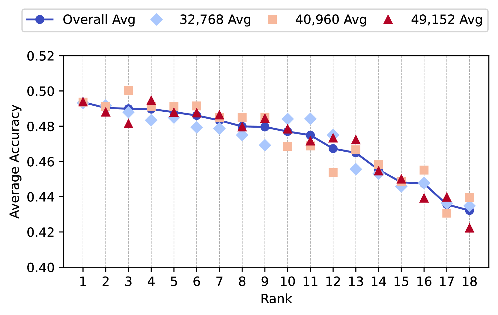</details> Figure 1: Effect of vocabulary size on downstream performance. For each tokenizer variant, we show the overall average, along with the three averages by vocabulary size, labeled according to the ranks in Table 1. Figure 1 gives the overall average, along with the individual averages, for each of the three vocabulary sizes for each variant, labeled according to the rank from Table 1. We observe that there is a high correlation between downstream performance at different vocabulary sizes. The pairwise $R^2$ values for the accuracy of the 32,768 and 40,960 runs was 0.750; between 40,960 and 49,152 it was 0.801; and between 32,768 and 49,152 it was 0.834. This corroborates the effect shown graphically in Figure 1 that vocabulary size is not a crucial decision over this range of sizes. Given this high degree of correlation, we focus our analysis on the overall average accuracy. This averaging removes some of the variance amongst individual language model runs. Thus, unless specified otherwise, our analyses present performance averaged over vocabulary sizes. ### 5.2 Overall performance To determine which of the differences in the overall average accuracy in Table 1 are statistically significant, we conduct a one-sided Wilcoxon signed-rank test Wilcoxon (1945) on the paired differences of the 30 accuracy scores (three vocabulary sizes over ten tasks), for each pair of variants. All $p$ -values reported in this paper use this test. <details> <summary>x2.png Details</summary>  ### Visual Description ## Heatmap: Statistical Significance (p-values) of Tokenizer Rank Comparisons ### Overview The image is a triangular heatmap visualizing p-values from statistical comparisons between tokenizers of different ranks. The chart displays a matrix where each cell represents the p-value resulting from a comparison between a tokenizer at a specific rank (x-axis) and a tokenizer at a lower rank (y-axis). The color intensity indicates the magnitude of the p-value, with a clear threshold at 0.05 for statistical significance. ### Components/Axes * **Chart Type:** Lower-triangular heatmap (the upper triangle is empty). * **X-Axis:** Labeled **"Tokenizer Rank"**. It has numerical markers from **1 to 18**, increasing from left to right. * **Y-Axis:** Labeled **"p-value vs. Lower Ranked Tokenizers"**. It has numerical markers from **1 to 18**, increasing from top to bottom. * **Color Scale/Legend:** Located on the right side. It is a vertical gradient bar labeled **"p-value"**. * The scale ranges from **0.00 (dark blue)** to **1.00 (dark red)**. * A critical threshold is marked at **0.05**, where the color transitions from shades of blue (p < 0.05) to shades of orange/red (p > 0.05). * Specific labeled ticks on the scale are: 0.00, 0.01, 0.02, 0.03, 0.04, 0.05, 0.10, 0.20, 0.30, 0.40, 0.50, 0.60, 0.70, 0.80, 0.90, 1.00. * **Visual Encoding:** * **Color:** Represents the p-value. Blue hues indicate low p-values (statistically significant difference), while orange/red hues indicate high p-values (no significant difference). * **Black Borders:** Certain cells are outlined with a thick black border. These borders are used to highlight specific cells, likely those with p-values below a certain threshold (e.g., p < 0.05) or of particular interest. ### Detailed Analysis The heatmap is a lower-triangular matrix, meaning it only shows comparisons where the rank on the y-axis is greater than or equal to the rank on the x-axis (i.e., comparing a higher-numbered rank to a lower-numbered rank). **Spatial and Color Pattern Analysis:** 1. **Top-Left Region (Ranks 1-6):** This area contains a mix of colors. Cells comparing very low ranks (e.g., Rank 1 vs. 2, Rank 2 vs. 3) show orange to red colors, indicating high p-values (p > 0.10, often > 0.30). This suggests no statistically significant difference between the performance of the very top-ranked tokenizers. Several of these cells have black borders. 2. **Diagonal and Near-Diagonal:** Cells comparing ranks that are close together (e.g., Rank 5 vs. 6, Rank 9 vs. 10) often show light orange or beige colors, with p-values frequently in the 0.10 to 0.40 range. Many of these cells are bordered in black. 3. **Bottom-Left Region (High y-rank vs. Low x-rank):** This large region is dominated by deep blue colors. For example, comparisons like Rank 18 vs. 1, Rank 15 vs. 2, or Rank 12 vs. 3 all show very dark blue, corresponding to p-values near **0.00 to 0.02**. This indicates a highly statistically significant difference when comparing a low-ranked tokenizer to a much higher-ranked one. 4. **Trend:** There is a clear gradient from the top-right (high p-values, red/orange) to the bottom-left (low p-values, blue). As the difference in rank between the two tokenizers being compared increases (moving down and to the left on the matrix), the p-value decreases dramatically. **Key Data Points (Approximate p-values from color):** * **Rank 1 vs. Rank 2:** p ≈ 0.60 - 0.70 (orange-red, bordered) * **Rank 2 vs. Rank 3:** p ≈ 0.50 - 0.60 (orange, bordered) * **Rank 5 vs. Rank 6:** p ≈ 0.20 - 0.30 (light orange, bordered) * **Rank 9 vs. Rank 10:** p ≈ 0.10 - 0.20 (beige, bordered) * **Rank 10 vs. Rank 11:** p ≈ 0.04 - 0.05 (light blue/grey, bordered) * **Rank 14 vs. Rank 15:** p ≈ 0.03 - 0.04 (light blue, bordered) * **Rank 17 vs. Rank 18:** p ≈ 0.10 - 0.20 (light orange, bordered) * **Rank 18 vs. Rank 1:** p ≈ 0.00 - 0.01 (dark blue) * **Rank 15 vs. Rank 3:** p ≈ 0.01 - 0.02 (dark blue) * **Rank 12 vs. Rank 5:** p ≈ 0.02 - 0.03 (medium blue) ### Key Observations 1. **Significant Hierarchy:** The data strongly suggests a performance hierarchy among the tokenizers. Tokenizers with lower rank numbers (1, 2, 3...) are not significantly different from each other (high p-values), but they are significantly different from tokenizers with much higher rank numbers (low p-values). 2. **Clustering at the Top:** The top 5-6 ranked tokenizers form a cluster where intra-group comparisons yield non-significant p-values. 3. **Clear Significance Threshold:** The color break at p=0.05 visually separates statistically significant comparisons (blue) from non-significant ones (orange/red). The black borders appear to primarily, but not exclusively, highlight cells with p-values near or above this threshold. 4. **Asymmetry:** The comparison is directional ("vs. Lower Ranked Tokenizers"). The heatmap only shows one direction of the pairwise comparison (e.g., Rank 5 vs. Rank 10 is shown, but Rank 10 vs. Rank 5 is not, as it would be in the empty upper triangle). ### Interpretation This heatmap is a statistical visualization tool likely used in machine learning or natural language processing research to evaluate tokenizer performance. The "Tokenizer Rank" probably corresponds to an ordering based on a performance metric (e.g., compression efficiency, downstream task accuracy). The data demonstrates that **performance differences are only statistically meaningful between tokenizers that are far apart in the ranking**. The top-performing tokenizers (ranks 1-6) are statistically indistinguishable from one another, forming a "top tier." However, any tokenizer in this top tier is significantly better than a tokenizer from the lower ranks (e.g., ranks 12-18). This suggests a plateau of performance at the top, with a clear drop-off to lower-performing models. The black borders likely serve to draw the viewer's attention to specific comparisons of interest, perhaps those that are "borderline" significant (p ≈ 0.05) or comparisons between adjacent ranks that the researchers wanted to highlight. The overall pattern validates the ranking system by showing that large rank differences correspond to large, statistically verifiable performance gaps. </details> Figure 2: Pairwise $p$ -values for 350M model results. Boxes outlined in black represent $p$ > 0.05. The top 6 tokenizers are all competitive, and there is no statistically significantly best approach. Figure 2 displays all pairwise $p$ -values in a color map. Each column designates a tokenization variant by its rank in Table 1, compared to all the ranks below it. A box is outlined in black if $p>0.05$ , where we cannot reject the null. While PathPieceL -BPE had the highest overall average on these tasks, the top five tokenizers, PathPieceL -BPE, Unigram, BPE, BPE-Greedy, and WordPiece do not have any other row in Figure 2 significantly different from them. Additionally, SaGe-BPE (rank 6) is only barely worse than PathPieceL -BPE ( $p$ = 0.047), and should probably be included in the list of competitive tokenizers. Thus, our first key result is that there is no tokenizer algorithm better than all others to a statistically significant degree. All the results reported thus far are for language models with identical architectures and 350M parameters. To examine the dependency on model size, we trained larger models of 1.3B parameters for six of our experiments, and 2.4B parameters for four of them. In the interest of computational time, these larger models were only trained with a single vocabulary size of 40,960. In Figure 6 in subsection 6.4, we report models’ average performance across 10 tasks. See Figure 7 in Appendix D for an example checkpoint graph at each model size. The main result from these models is that the relative performance of the tokenizers does vary by model size, and that there is a group of high performing tokenizers that yield comparable results. This aligns with our finding that the top six tokenizers are not statistically better than one another at the 350M model size. 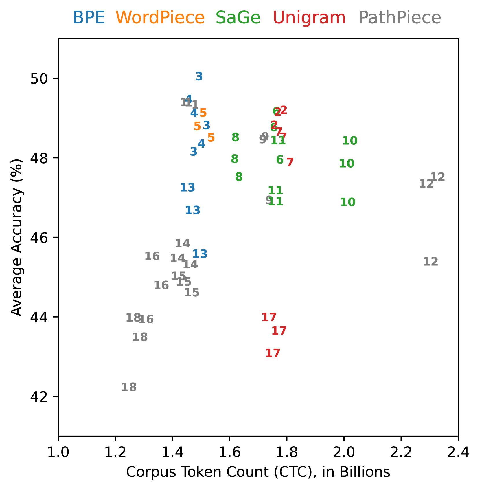### 5.3 Corpus Token Count vs Accuracy Figure 3 shows the corpus token count (CTC) versus the accuracy of each vocabulary size, given in Table 11. We do not find a straightforward relationship between the two. Ali et al. (2024) recently examined the relationship between CTC and downstream performance for three different tokenizers, and also found it was not correlated on English language tasks. <details> <summary>x3.png Details</summary>  ### Visual Description \n ## Scatter Plot: Tokenization Method Performance vs. Corpus Token Count ### Overview This image is a scatter plot comparing the performance of five different tokenization methods. The chart plots "Average Accuracy (%)" against "Corpus Token Count (CTC), in Billions." Each data point is labeled with a number, likely representing a specific configuration or experiment ID for that method. The data points are color-coded according to the tokenization method, as indicated by the legend at the top of the chart. ### Components/Axes * **Y-Axis:** Labeled "Average Accuracy (%)". The scale runs from 42 to 50, with major tick marks at 42, 44, 46, 48, and 50. * **X-Axis:** Labeled "Corpus Token Count (CTC), in Billions". The scale runs from 1.0 to 2.4, with major tick marks at 1.0, 1.2, 1.4, 1.6, 1.8, 2.0, 2.2, and 2.4. * **Legend:** Positioned at the top-center of the chart, above the plot area. It lists five tokenization methods, each associated with a specific color: * **BPE** (Blue) * **WordPiece** (Orange) * **SaGe** (Green) * **Unigram** (Red) * **PathPiece** (Gray) * **Data Points:** Each point on the scatter plot is represented by a colored number. The number corresponds to a specific experiment or configuration for the method indicated by its color. ### Detailed Analysis The plot reveals distinct clustering and ranges for each tokenization method: * **BPE (Blue):** Points are clustered in a relatively narrow band of Corpus Token Count (CTC), approximately between 1.4 and 1.6 billion. Their Average Accuracy ranges from about 46% to 50%. The highest accuracy point on the entire chart (≈50%) belongs to BPE (labeled "3"). * **WordPiece (Orange):** Points are tightly clustered near a CTC of 1.5 billion, with Average Accuracy between approximately 48% and 49%. * **SaGe (Green):** Points are spread across a wider CTC range, from about 1.6 to 2.0 billion. Their Average Accuracy is generally high, clustering between 47% and 49%. * **Unigram (Red):** Points are found in two distinct clusters. One cluster is at a CTC of approximately 1.7-1.8 billion with high accuracy (≈49%). A second, separate cluster is at a similar CTC (≈1.7-1.8 billion) but with significantly lower accuracy, between 43% and 44% (points labeled "17"). * **PathPiece (Gray):** This method shows the widest dispersion. Points are scattered across nearly the entire X-axis range, from a CTC of ~1.2 billion to ~2.3 billion. Correspondingly, its Average Accuracy varies dramatically, from a low of ~42% (point "18" at ~1.2 billion CTC) to a high of ~49% (points "11" and "12" at ~1.4 and ~2.3 billion CTC, respectively). ### Key Observations 1. **Performance-Accuracy Trade-off:** There is no simple linear trade-off between Corpus Token Count and Average Accuracy. High accuracy can be achieved across a range of CTC values (1.4 to 2.0 billion) by different methods. 2. **Method-Specific Clustering:** Each method (except PathPiece) occupies a somewhat distinct region of the plot, suggesting inherent characteristics in how they tokenize data, affecting both count and resulting model accuracy. 3. **Unigram Bimodality:** The Unigram method exhibits a clear bimodal distribution, with one group performing at the top tier of accuracy and another group performing near the bottom. This suggests the existence of two very different configurations or outcomes for this method. 4. **PathPiece Variability:** PathPiece demonstrates the highest variance in both metrics, indicating its performance is highly sensitive to its configuration or the specific task/data it's applied to. 5. **Peak Performance Zone:** The highest density of high-accuracy points (>48%) occurs within a CTC range of approximately 1.4 to 1.8 billion tokens. ### Interpretation This chart visualizes the complex relationship between tokenization strategy, the resulting compressed representation of a text corpus (CTC), and the downstream task performance (Average Accuracy). It demonstrates that there is no single "best" tokenizer; the optimal choice depends on the desired balance between compression efficiency (lower CTC) and model accuracy. The clustering suggests that methods like BPE and WordPiece offer predictable, high-performance outcomes within a specific operational range. SaGe provides a good balance, maintaining high accuracy even with a moderately higher token count. The stark split in Unigram's results is particularly noteworthy, implying that its performance is not robust and can fail dramatically under certain conditions. PathPiece's wide scatter positions it as a potentially high-risk, high-reward option, capable of both the worst and some of the best results, requiring careful tuning. From a research perspective, this plot argues against evaluating tokenizers on a single metric. A comprehensive assessment must consider both the efficiency of the tokenization (CTC) and its impact on model quality (Accuracy). The outliers, like the low-accuracy Unigram cluster and the low-CTC/low-accuracy PathPiece points, are critical for understanding the failure modes of these algorithms. </details> Figure 3: Effect of corpus token count (CTC) vs average accuracy of individual vocabulary sizes. The two models with the highest CTC are PathPiece with Space pre-tokenization (12), which is to be expected given each space is its own token, and SaGe with an initial Unigram vocabulary (10). The Huggingface Unigram models in Figure 3 had significantly higher CTC than the corresponding BPE models, unlike Bostrom and Durrett (2020) and Gow-Smith et al. (2022), which report a difference of only a few percent with SentencePiece Unigram. Ali et al. (2024) point out that due to differences in pre-processing, the Huggingface Unigram tokenizer behaves quite differently than the SentencePiece Unigram tokenizer, which may explain this discrepancy. In terms of accuracy, PathPiece with no pre-tokenization (18) and Unigram with PathPiece segmentation (17) both did quite poorly. Notably, the range of CTC is quite narrow within each vocabulary construction method, even while changes in pre-tokenization and segmentation lead to significant accuracy differences. While there are confounding factors present in this chart (e.g., pre-tokenization, vocabulary initialization, and that more tokens allow for additional computations by the downstream model) it is difficult to discern any trend that lower CTC leads to improved performance. If anything, there seems to be an inverted U-shaped curve with respect to the CTC and downstream performance. The Pearson correlation coefficient between CTC and average accuracy was found to be 0.241. Given that a lower CTC value signifies greater compression, this result suggests a weak negative relationship between the amount of compression and average accuracy. Zouhar et al. (2023a) introduced an information-theoretic measure based on Rényi efficiency that correlates with downstream performance for their application. Except, so far, for a family of adversarially-created tokenizers Cognetta et al. (2024). It has an order parameter $α$ , with a recommended value of 2.5. We present the Rényi efficiencies and CTC for all models in Table 11 in Appendix G, and summarize their Pearson correlation with average accuracy in Table 2. For the data of Figure 3, all the correlations for various $α$ also have a weak negative association. They are slightly less negative than the association for CTC, although it is not nearly as large as the benefit they saw over sequence length in their application. We note the strong relationship between compression and Rényi efficiency, as the Pearson correlation of CTC and Rényi efficiency with $α$ =2.5 is $-$ 0.891. | CTC and Ave Acc Rényi Eff and Ave Acc ( $α$ =1.5) Rényi Eff and Ave Acc ( $α$ =2.0) | 0.241 $-$ 0.221 $-$ 0.169 | | --- | --- | | Rényi Eff and Ave Acc ( $α$ =2.5) | $-$ 0.151 | | Rényi Eff and Ave Acc ( $α$ =3.0) | $-$ 0.144 | | Rényi Eff and Ave Acc ( $α$ =3.5) | $-$ 0.141 | | CTC and Rényi Eff ( $α$ =2.5) | $-$ 0.891 | Table 2: Pearson Correlation of CTC and Average Accuracy, or Rényi efficiency for various orders $α$ with Average Accuracy, or CTC and Rényi efficiency at $α=2.5$ . By varying aspects of BPE, Gallé (2019) and Goldman et al. (2024) suggests we should expect downstream performance to decrease with CTC, while in contrast Ali et al. (2024) did not find a strong relation when varying the tokenizer. Our extensive results varying a number of stages of tokenization suggest it is not inherently beneficial to use fewer tokens. Rather, the particular way that the CTC is varied can lead to different conclusions. ## 6 Analysis We now analyze the results across the various experiments in a more controlled manner. Our experiments allow us to examine changes in each stage of tokenization, holding the rest constant, revealing design decisions making a significant difference. Appendix E contains additional analysis ### 6.1 Pre-tokenization For PathPieceR with an $n$ -gram initial vocabulary, we can isolate pre-tokenization. PathPiece is efficient enough to process entire documents with no pre-tokenization, giving it full freedom to minimize the corpus token count (CTC). | 12 14 18 | SpaceDigit FirstSpDigit None | The ␣ valuation ␣ is ␣ estimated ␣ to ␣ be ␣ $ 2 1 3 M The ␣valuation ␣is ␣estimated ␣to ␣be ␣$ 2 1 3 M The ␣valu ation␣is ␣estimated ␣to␣b e␣$ 2 1 3 M | | --- | --- | --- | Table 3: Example PathPiece tokenizations of “The valuation is estimated to be $213M”; vocabulary size of 32,768. 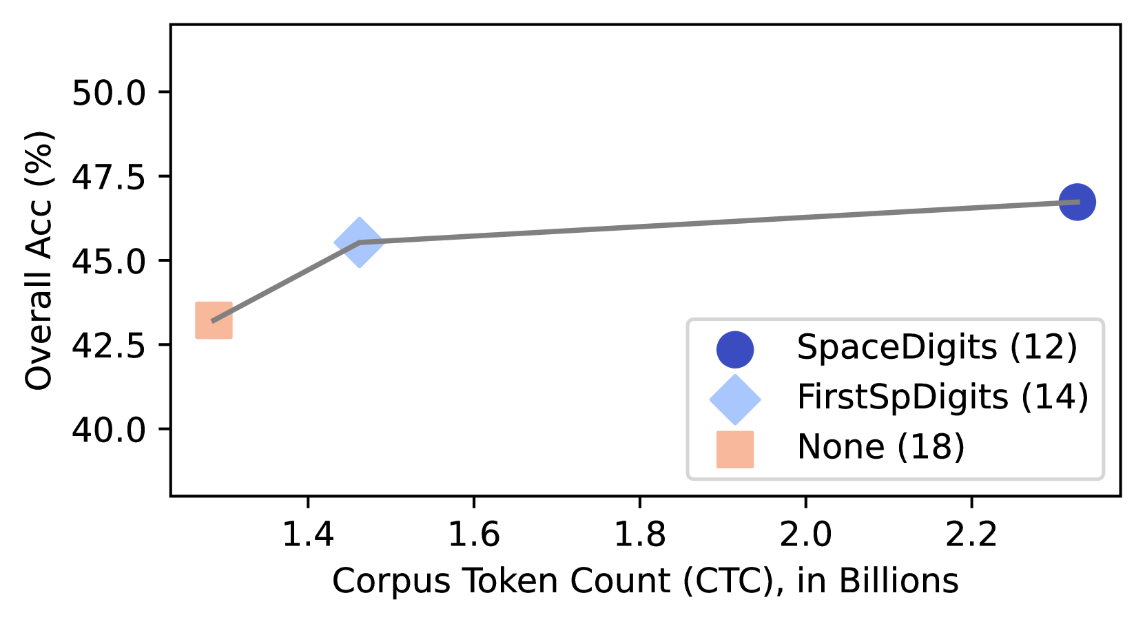Adding pre-tokenization constrains PathPiece ’s ability to minimize tokens, giving a natural way to vary the number of tokens. Figure 4 shows that PathPiece minimizes the number of tokens used over a corpus when trained with no pre-tokenization (18). The other variants restrict spaces to either be the first character of a token (14), or their own token (12). These two runs also used Digit pre-tokenization where each digit is its own token. Consider the example PathPiece tokenization in Table 3 for the three pre-tokenization methods. The None mode uses the word-boundary-spanning tokens “ ation␣is ”, “ ␣to␣b ”, and “ e␣$ ”. The lack of morphological alignment demonstrated in this example is likely more important to downstream model performance than a simple token count. In Figure 4 we observe a statistically significant increase in overall accuracy for our downstream tasks, as a function of CTC. Gow-Smith et al. (2022) found that Space pre-tokenization lead to worse performance, while removing the spaces entirely helps Although omitting the spaces entirely does not lead to a reversible tokenization as we have been considering.. Thus, this particular result may be specific to PathPieceR. <details> <summary>x4.png Details</summary>  ### Visual Description \n ## Line Chart: Corpus Token Count vs. Overall Accuracy ### Overview This is a line chart plotting the relationship between the size of a training corpus (in billions of tokens) and the resulting overall accuracy percentage for three different methods or models. The chart shows a positive correlation: as the Corpus Token Count (CTC) increases, the Overall Accuracy generally increases. ### Components/Axes * **X-Axis (Horizontal):** * **Label:** "Corpus Token Count (CTC), in Billions" * **Scale:** Linear scale. * **Major Tick Marks:** 1.4, 1.6, 1.8, 2.0, 2.2. * **Range:** Approximately 1.3 to 2.35 billion tokens. * **Y-Axis (Vertical):** * **Label:** "Overall Acc (%)" * **Scale:** Linear scale. * **Major Tick Marks:** 40.0, 42.5, 45.0, 47.5, 50.0. * **Range:** 40.0% to 50.0%. * **Legend (Bottom-Right Corner):** * **Position:** Located in the bottom-right quadrant of the chart area. * **Entries:** 1. **Dark Blue Circle:** "SpaceDigits (12)" 2. **Light Blue Diamond:** "FirstSpDigits (14)" 3. **Light Orange Square:** "None (18)" * **Note:** The numbers in parentheses (12, 14, 18) are part of the legend labels but their specific meaning (e.g., model size, parameter count) is not defined in the chart. ### Detailed Analysis The chart contains three distinct data points connected by a single grey line, indicating they belong to the same series or experimental progression. 1. **Data Point 1 (Light Orange Square - "None (18)"):** * **Spatial Position:** Leftmost point. * **X-Value (CTC):** Approximately 1.3 billion tokens. * **Y-Value (Accuracy):** Approximately 43.0%. * **Trend Context:** This is the lowest accuracy point, corresponding to the smallest corpus size. 2. **Data Point 2 (Light Blue Diamond - "FirstSpDigits (14)"):** * **Spatial Position:** Center-left. * **X-Value (CTC):** Approximately 1.45 billion tokens. * **Y-Value (Accuracy):** Approximately 45.5%. * **Trend Context:** A significant increase in accuracy (~2.5 percentage points) is observed with a relatively small increase in corpus size (~0.15 billion tokens) from the first point. 3. **Data Point 3 (Dark Blue Circle - "SpaceDigits (12)"):** * **Spatial Position:** Rightmost point. * **X-Value (CTC):** Approximately 2.3 billion tokens. * **Y-Value (Accuracy):** Approximately 46.8%. * **Trend Context:** This point represents the highest accuracy and the largest corpus size. The slope of the line between the second and third points is less steep than between the first and second, suggesting diminishing returns. **Trend Verification:** The connecting line slopes upward from left to right, confirming a positive trend between CTC and Accuracy. The steepest slope occurs between the "None" and "FirstSpDigits" points. ### Key Observations * **Positive Correlation:** There is a clear, monotonic increase in Overall Accuracy as the Corpus Token Count increases across the three data points. * **Diminishing Returns:** The gain in accuracy per additional billion tokens appears to decrease. Moving from ~1.3B to ~1.45B tokens yields a ~2.5% accuracy gain, while moving from ~1.45B to ~2.3B tokens (a much larger increase of ~0.85B tokens) yields only a ~1.3% gain. * **Method/Model Identification:** The legend links specific accuracy/CTC combinations to named methods ("None", "FirstSpDigits", "SpaceDigits") and an associated number in parentheses. The "SpaceDigits (12)" method achieves the highest accuracy but requires a corpus more than 50% larger than the "FirstSpDigits (14)" method for a modest performance improvement. ### Interpretation The data suggests that increasing the volume of training data (Corpus Token Count) is an effective strategy for improving the overall accuracy of the system or model being tested. However, the relationship is not linear; the most significant efficiency gains (accuracy per token) are achieved at lower corpus sizes. The named methods in the legend likely represent different data preprocessing, augmentation, or model architecture techniques. The chart implies a trade-off: the "SpaceDigits" method, while achieving peak performance, is less data-efficient than "FirstSpDigits." The number in parentheses could indicate a model size (e.g., 12B parameters vs. 14B), suggesting that a smaller model ("SpaceDigits (12)") trained on vastly more data can outperform a larger model ("FirstSpDigits (14)") trained on less data. This highlights a critical consideration in machine learning: the balance between model capacity and data scale. The "None" baseline performs worst, establishing the value of the applied techniques. </details> Figure 4: The impact of pre-tokenization on Corpus Token Count (CTC) and Overall Accuracy. Ranks in parentheses refer to performance in Table 1. 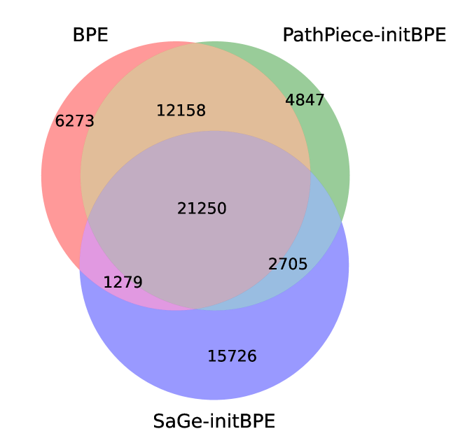### 6.2 Vocabulary Construction One way to examine the effects of vocabulary construction is to compare the resulting vocabularies of top-down methods trained using an initial vocabulary to the method itself. Figure 5 presents an area-proportional Venn diagram of the overlap in 40,960-sized vocabularies between BPE (6) and variants of PathPieceL (1) and SaGe (6) that were trained using an initial BPE vocabulary of size $2^18=262,144$ . See Figure 12 in Appendix E.3 for analogous results for Unigram, which behaves similarly. While BPE and PathPieceL overlap considerably, SaGe produces a more distinct set of tokens. <details> <summary>x5.png Details</summary>  ### Visual Description \n ## Venn Diagram: Tokenization Method Overlap ### Overview This image is a three-set Venn diagram illustrating the overlap and unique elements between three different tokenization or data processing methods: **BPE**, **PathPiece-initBPE**, and **SaGe-initBPE**. The diagram quantifies the number of items (likely tokens, subwords, or data points) that are exclusive to each method and those shared between two or all three methods. ### Components/Axes * **Sets (Circles):** * **BPE:** Represented by a red circle positioned in the top-left quadrant. * **PathPiece-initBPE:** Represented by a green circle positioned in the top-right quadrant. * **SaGe-initBPE:** Represented by a blue circle positioned in the bottom-center. * **Labels:** Each circle is labeled with its method name in black text, placed outside the circle near its top edge. * **Data Points:** Numerical values are placed directly within each distinct segment of the diagram, indicating the count for that specific intersection or unique set. ### Detailed Analysis The diagram is divided into seven distinct regions, each with a specific count: 1. **BPE Only (Red, non-overlapping):** `6273` 2. **PathPiece-initBPE Only (Green, non-overlapping):** `4847` 3. **SaGe-initBPE Only (Blue, non-overlapping):** `15726` 4. **BPE ∩ PathPiece-initBPE (Red-Green overlap, excluding blue):** `12158` 5. **PathPiece-initBPE ∩ SaGe-initBPE (Green-Blue overlap, excluding red):** `2705` 6. **BPE ∩ SaGe-initBPE (Red-Blue overlap, excluding green):** `1279` 7. **BPE ∩ PathPiece-initBPE ∩ SaGe-initBPE (Central, all three overlap):** `21250` **Spatial Grounding & Color Verification:** * The number `6273` is placed in the red-only segment of the BPE circle (top-left). * The number `4847` is placed in the green-only segment of the PathPiece-initBPE circle (top-right). * The number `15726` is placed in the blue-only segment of the SaGe-initBPE circle (bottom-center). * The number `12158` is in the overlapping area of the red (BPE) and green (PathPiece-initBPE) circles, which appears as a tan/brown color. * The number `2705` is in the overlapping area of the green (PathPiece-initBPE) and blue (SaGe-initBPE) circles, which appears as a light blue/cyan color. * The number `1279` is in the overlapping area of the red (BPE) and blue (SaGe-initBPE) circles, which appears as a purple/magenta color. * The number `21250` is in the central region where all three circles (red, green, blue) overlap, appearing as a muted purple/grey. ### Key Observations 1. **Largest Unique Set:** The **SaGe-initBPE** method has the highest number of unique elements (`15726`), significantly more than BPE (`6273`) or PathPiece-initBPE (`4847`). 2. **Largest Overlap:** The largest intersection is the central region common to all three methods (`21250`), indicating a substantial core set of elements shared by all approaches. 3. **Pairwise Overlap Disparity:** The overlap between BPE and PathPiece-initBPE (`12158`) is much larger than the overlap between PathPiece-initBPE & SaGe-initBPE (`2705`) or BPE & SaGe-initBPE (`1279`). This suggests BPE and PathPiece-initBPE are more similar to each other than either is to SaGe-initBPE. 4. **Smallest Overlap:** The intersection between BPE and SaGe-initBPE (`1279`) is the smallest, highlighting these two methods as the most distinct pair in terms of their exclusive shared elements. ### Interpretation This Venn diagram provides a quantitative comparison of three tokenization strategies, likely from a natural language processing or machine learning context. The data suggests: * **Common Foundation:** A large core set of over 21,000 elements is fundamental to all three methods, representing a common vocabulary or data structure. * **Methodological Divergence:** SaGe-initBPE appears to be the most distinct method, with a large proprietary set of elements (`15726`) and relatively small overlaps with the other two. This could indicate it captures different linguistic features or uses a different initialization strategy. * **BPE and PathPiece Similarity:** The significant overlap between BPE and PathPiece-initBPE implies that PathPiece-initBPE may be an evolution or variant of standard BPE, retaining a large portion of its core elements while adding its own unique set (`4847`). * **Practical Implications:** For a practitioner, this diagram helps answer questions like: "If I switch from BPE to SaGe-initBPE, how much of my existing vocabulary will be preserved?" (Answer: `1279 + 21250 = 22529` elements are shared). It also visually argues that SaGe-initBPE introduces the most novel elements into the ecosystem. </details> Figure 5: Venn diagram comparing 40,960 token vocabularies of BPE, PathPieceL and SaGe – the latter two were both initialized from a BPE vocabulary of 262,144. ### 6.3 Initial Vocabulary PathPiece, SaGe, and Unigram all require an initial vocabulary. The HuggingFace Unigram implementation starts with the one millionp $n$ -grams, but sorted according to the count times the length of the token, introducing a bias toward longer tokens. For PathPiece and SaGe, we experimented with initial vocabularies of size 262,144 constructed from either the most frequent $n$ -grams, or trained using either BPE or Unigram. For PathPieceL, using a BPE initial vocabulary (1) is statistically better than both Unigram (9) and $n$ -grams (16), with $p≤ 0.01$ . Using an $n$ -gram initial vocabulary leads to the lowest performance, with statistical significance. Comparing ranks 6, 8, and 10 reveals the same pattern for SaGe, although the difference between 8 and 10 is not significant. 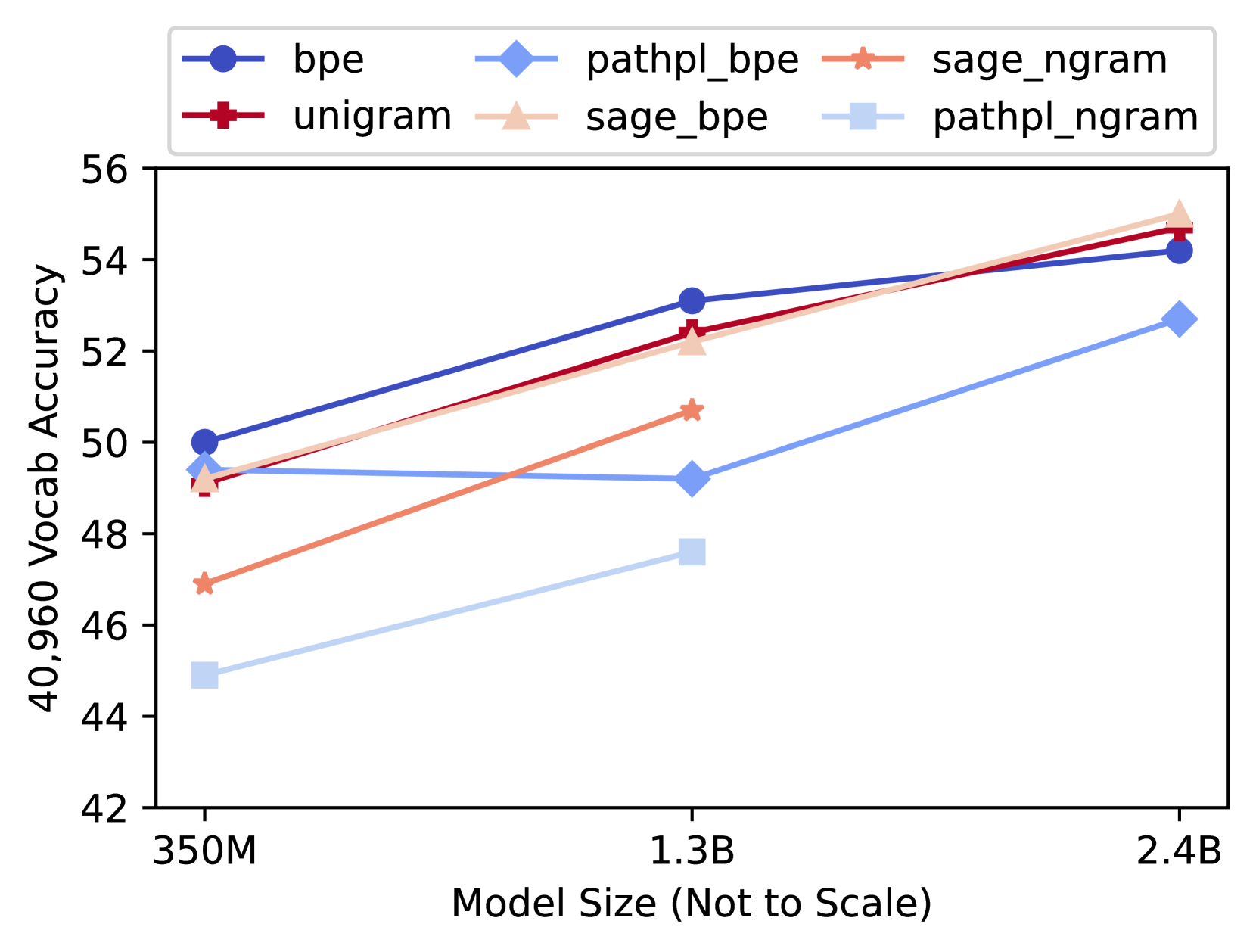### 6.4 Effect of Model Size To examine the dependency on model size, we build larger models of 1.3B parameters for 6 of our experiments, and 2.4B parameters for 4 of them. These models were trained over the same 200 billion tokens. In the interest of computational time, these larger models were only run at a single vocabulary size of 40,960. The average results over the 10 task accuracies for these models is given in Figure 6. See Table 14 in Appendix G for the numerical values. <details> <summary>x6.png Details</summary>  ### Visual Description ## Line Chart: Model Size vs. Vocab Accuracy for Different Tokenization Methods ### Overview The image is a line chart comparing the performance of six different tokenization or model training methods across three model sizes. The chart plots "40,960 Vocab Accuracy" on the y-axis against "Model Size (Not to Scale)" on the x-axis. The data suggests that accuracy generally increases with model size for all methods, but the rate of improvement and final performance vary significantly. ### Components/Axes * **Chart Type:** Multi-series line chart. * **Y-Axis:** * **Label:** "40,960 Vocab Accuracy" * **Scale:** Linear, ranging from 42 to 56, with major tick marks every 2 units (42, 44, 46, 48, 50, 52, 54, 56). * **X-Axis:** * **Label:** "Model Size (Not to Scale)" * **Categories/Points:** Three discrete model sizes: "350M", "1.3B", "2.4B". The axis is categorical, not numerically scaled. * **Legend:** Positioned at the top center of the chart area. It contains six entries, each with a unique color, line style, and marker: 1. `bpe`: Dark blue line with circle markers. 2. `unigram`: Dark red line with square markers. 3. `pathpl_bpe`: Light blue line with diamond markers. 4. `sage_bpe`: Light orange/peach line with upward-pointing triangle markers. 5. `sage_ngram`: Orange line with star (asterisk) markers. 6. `pathpl_ngram`: Very light blue/grey line with square markers. ### Detailed Analysis **Data Series Trends and Approximate Values:** 1. **bpe (Dark Blue, Circles):** * **Trend:** Steady, strong upward slope across all model sizes. * **Values:** ~50.0 (350M) → ~53.1 (1.3B) → ~54.2 (2.4B). 2. **unigram (Dark Red, Squares):** * **Trend:** Strong upward slope, nearly parallel to `bpe` but slightly lower at 350M and 1.3B, converging at 2.4B. * **Values:** ~49.1 (350M) → ~52.5 (1.3B) → ~54.7 (2.4B). 3. **sage_bpe (Light Orange, Triangles):** * **Trend:** Very strong upward slope, starting near `unigram` and ending as the highest-performing method at 2.4B. * **Values:** ~49.2 (350M) → ~52.2 (1.3B) → ~55.0 (2.4B). 4. **sage_ngram (Orange, Stars):** * **Trend:** Moderate upward slope. Data is only plotted for 350M and 1.3B; the line does not extend to 2.4B. * **Values:** ~46.9 (350M) → ~50.7 (1.3B). No data point for 2.4B. 5. **pathpl_bpe (Light Blue, Diamonds):** * **Trend:** Slight dip or plateau between 350M and 1.3B, followed by a strong increase to 2.4B. * **Values:** ~49.4 (350M) → ~49.2 (1.3B) → ~52.7 (2.4B). 6. **pathpl_ngram (Very Light Blue, Squares):** * **Trend:** Steady upward slope. This is the lowest-performing series at 350M and 1.3B. Data is only plotted for these two points. * **Values:** ~44.9 (350M) → ~47.6 (1.3B). No data point for 2.4B. ### Key Observations * **Performance Hierarchy at 350M:** `bpe` > `pathpl_bpe` ≈ `sage_bpe` ≈ `unigram` > `sage_ngram` > `pathpl_ngram`. * **Performance Hierarchy at 1.3B:** `bpe` > `unigram` > `sage_bpe` > `sage_ngram` > `pathpl_bpe` > `pathpl_ngram`. * **Performance Hierarchy at 2.4B:** `sage_bpe` > `unigram` > `bpe` > `pathpl_bpe`. (`sage_ngram` and `pathpl_ngram` have no data). * **Notable Outliers/Anomalies:** * `pathpl_bpe` is the only method that does not show a strict monotonic increase, exhibiting a slight performance drop when scaling from 350M to 1.3B. * The `sage_ngram` and `pathpl_ngram` methods have incomplete data, missing results for the largest (2.4B) model size. * At the largest model size (2.4B), the `sage_bpe` method overtakes the initially leading `bpe` method. ### Interpretation This chart demonstrates the relationship between model scale and downstream task accuracy (specifically for a 40,960 vocabulary size) when using different subword tokenization or training strategies. The core finding is that **increasing model size generally improves accuracy**, but the choice of tokenization method significantly impacts both the absolute performance and the scaling efficiency. * **Method Effectiveness:** The `sage_bpe` and `unigram` methods show the most promising scaling behavior, with `sage_bpe` achieving the highest observed accuracy at 2.4B parameters. The standard `bpe` method is a strong and consistent performer but is eventually surpassed. * **Scaling Inefficiency:** The `pathpl_bpe` method's dip at 1.3B suggests a potential instability or suboptimal configuration at that specific scale, though it recovers at 2.4B. The `pathpl_ngram` method consistently underperforms others at the scales where it is measured. * **Data Gaps:** The absence of data for `sage_ngram` and `pathpl_ngram` at 2.4B limits a full comparison. It is unclear if this is due to experimental constraints, failure to converge, or results not being ready. * **Practical Implication:** For practitioners aiming to maximize accuracy with a large vocabulary, this data suggests that `sage_bpe` or `unigram` tokenization paired with a model size of at least 2.4B parameters is a highly effective combination. The choice between methods may also depend on other factors not shown here, such as training cost, inference speed, or performance on other metrics. </details> Figure 6: 40,960 vocab average accuracy at various models sizes It is noteworthy from the prevalence of crossing lines in Figure 6 that the relative performance of the tokenizers do vary by model size, and that there is a group of tokenizers that are trading places being at the top for various model sizes. This aligns with our observation that the top 6 tokenizers were within the noise, and not significantly better than each other in the 350M models. ## 7 Conclusion We investigate the hypothesis that reducing the corpus token count (CTC) would improve downstream performance, as suggested by Gallé (2019) and Goldman et al. (2024) when they varied aspects of BPE. When comparing CTC and downstream accuracy across all our experimental settings in Figure 3, we do not find a clear relationship between the two. We expand on the findings of Ali et al. (2024) who did not find a strong relation when comparing 3 tokenizers, as we run 18 experiments varying the tokenizer, initial vocabulary, pre-tokenizer, and inference method. Our results suggest compression is not a straightforward explanation of what makes a tokenizer effective. Finally, this work makes several practical contributions: (1) vocabulary size has little impact on downstream performance over the range of sizes we examined (§ 5.1); (2) five different tokenizers all perform comparably, with none outperforming at statistical significance (§ 5.2); (3) BPE initial vocabularies work best for top-down vocabulary construction (§ 6.3). To further encourage research in this direction, we make all of our trained vocabularies publicly available, along with the model weights from our 64 language models. ## Limitations The objective of this work is to offer a comprehensive analysis of the tokenization process. However, our findings were constrained to particular tasks and models. Given the degrees of freedom, such as choice of downstream tasks, model, vocabulary size, etc., there is a potential risk of inadvertently considering our results as universally applicable to all NLP tasks; results may not generalize to other domains of tasks. Additionally, our experiments were exclusively with English language text, and it is not clear how these results will extend to other languages. In particular, our finding that pre-tokenization is crucial for effective downstream accuracy is not applicable to languages without space-delimited words. We conducted experiments for three district vocabulary sizes, and we reported averaged results across these experiments. With additional compute resources and time, it could be beneficial to conduct further experiments to gain a better estimate of any potential noise. For example, in Figure 7 of Appendix D, the 100k checkpoint at the 1.3B model size is worse than expected, indicating that noise could be an issue. Finally, the selection of downstream tasks can have a strong impact on results. To allow for meaningful results, we attempted to select tasks that were neither too difficult nor too easy for the 350M parameter models, but other choices could lead to different outcomes. There does not seem to be a good, objective criteria for selecting a finite set of task to well-represent global performance. ## Ethics Statement We have used the commonly used public dataset The Pile, which has not undergone a formal ethics review Biderman et al. (2022). Our models may include biases from the training data. Our experimentation has used considerable energy. Each 350M parameter run took approximately 48 hours on (4) p4de nodes, each containing 8 NVIDIA A100 GPUs. We trained 62 models, including the 8 RandTrain runs in Appendix F. The (6) 1.3B parameters models took approximately 69 hours to train on (4) p4de nodes, while the (4) 2.4B models took approximately 117 hours to train on (8) p4de nodes. In total, training required 17,304 hours of p4de usage (138,432 GPU hours). ## Acknowledgments Thanks to Charles Lovering at Kensho for his insightful suggestions, and to Michael Krumdick, Mike Arov, and Brian Chen at Kensho for their help with the language model development process. This research was supported in part by the Israel Science Foundation (grant No. 1166/23). Thanks to an anonymous reviewer who pointed out the large change in CTC when comparing Huggingface BPE and Unigram, in contrast to the previous literature using the SentencePiece implementations Kudo and Richardson (2018). ## References - Ali et al. (2024) Mehdi Ali, Michael Fromm, Klaudia Thellmann, Richard Rutmann, Max Lübbering, Johannes Leveling, Katrin Klug, Jan Ebert, Niclas Doll, Jasper Schulze Buschhoff, Charvi Jain, Alexander Arno Weber, Lena Jurkschat, Hammam Abdelwahab, Chelsea John, Pedro Ortiz Suarez, Malte Ostendorff, Samuel Weinbach, Rafet Sifa, Stefan Kesselheim, and Nicolas Flores-Herr. 2024. Tokenizer choice for llm training: Negligible or crucial? - Amini et al. (2019) Aida Amini, Saadia Gabriel, Peter Lin, Rik Koncel-Kedziorski, Yejin Choi, and Hannaneh Hajishirzi. 2019. Mathqa: Towards interpretable math word problem solving with operation-based formalisms. - Bauwens and Delobelle (2024) Thomas Bauwens and Pieter Delobelle. 2024. BPE-knockout: Pruning pre-existing BPE tokenisers with backwards-compatible morphological semi-supervision. In Proceedings of the 2024 Conference of the North American Chapter of the Association for Computational Linguistics: Human Language Technologies (Volume 1: Long Papers), pages 5810–5832, Mexico City, Mexico. Association for Computational Linguistics. - Biderman et al. (2022) Stella Biderman, Kieran Bicheno, and Leo Gao. 2022. Datasheet for the pile. CoRR, abs/2201.07311. - Bisk et al. (2019) Yonatan Bisk, Rowan Zellers, Ronan Le Bras, Jianfeng Gao, and Yejin Choi. 2019. Piqa: Reasoning about physical commonsense in natural language. - Bostrom and Durrett (2020) Kaj Bostrom and Greg Durrett. 2020. Byte pair encoding is suboptimal for language model pretraining. In Findings of the Association for Computational Linguistics: EMNLP 2020, pages 4617–4624, Online. Association for Computational Linguistics. - Bouma (2009) Gerlof Bouma. 2009. Normalized (pointwise) mutual information in collocation extraction. Proceedings of GSCL, 30:31–40. - Brassard et al. (2022) Ana Brassard, Benjamin Heinzerling, Pride Kavumba, and Kentaro Inui. 2022. Copa-sse: Semi-structured explanations for commonsense reasoning. - Chizhov et al. (2024) Pavel Chizhov, Catherine Arnett, Elizaveta Korotkova, and Ivan P. Yamshchikov. 2024. Bpe gets picky: Efficient vocabulary refinement during tokenizer training. - Clark et al. (2018) Peter Clark, Isaac Cowhey, Oren Etzioni, Tushar Khot, Ashish Sabharwal, Carissa Schoenick, and Oyvind Tafjord. 2018. Think you have solved question answering? try arc, the ai2 reasoning challenge. ArXiv, abs/1803.05457. - Cognetta et al. (2024) Marco Cognetta, Vilém Zouhar, Sangwhan Moon, and Naoaki Okazaki. 2024. Two counterexamples to tokenization and the noiseless channel. In Proceedings of the 2024 Joint International Conference on Computational Linguistics, Language Resources and Evaluation (LREC-COLING 2024), pages 16897–16906, Torino, Italia. ELRA and ICCL. - Efraimidis (2010) Pavlos S. Efraimidis. 2010. Weighted random sampling over data streams. CoRR, abs/1012.0256. - Gage (1994) Philip Gage. 1994. A new algorithm for data compression. C Users J., 12(2):23–38. - Gallé (2019) Matthias Gallé. 2019. Investigating the effectiveness of BPE: The power of shorter sequences. In Proceedings of the 2019 Conference on Empirical Methods in Natural Language Processing and the 9th International Joint Conference on Natural Language Processing (EMNLP-IJCNLP), pages 1375–1381, Hong Kong, China. Association for Computational Linguistics. - Gao et al. (2020) Leo Gao, Stella Biderman, Sid Black, Laurence Golding, Travis Hoppe, Charles Foster, Jason Phang, Horace He, Anish Thite, Noa Nabeshima, Shawn Presser, and Connor Leahy. 2020. The pile: An 800gb dataset of diverse text for language modeling. - Gao et al. (2023) Leo Gao, Jonathan Tow, Baber Abbasi, Stella Biderman, Sid Black, Anthony DiPofi, Charles Foster, Laurence Golding, Jeffrey Hsu, Alain Le Noac’h, Haonan Li, Kyle McDonell, Niklas Muennighoff, Chris Ociepa, Jason Phang, Laria Reynolds, Hailey Schoelkopf, Aviya Skowron, Lintang Sutawika, Eric Tang, Anish Thite, Ben Wang, Kevin Wang, and Andy Zou. 2023. A framework for few-shot language model evaluation. - Goldman et al. (2024) Omer Goldman, Avi Caciularu, Matan Eyal, Kris Cao, Idan Szpektor, and Reut Tsarfaty. 2024. Unpacking tokenization: Evaluating text compression and its correlation with model performance. - Gow-Smith et al. (2024) Edward Gow-Smith, Dylan Phelps, Harish Tayyar Madabushi, Carolina Scarton, and Aline Villavicencio. 2024. Word boundary information isn’t useful for encoder language models. In Proceedings of the 9th Workshop on Representation Learning for NLP (RepL4NLP-2024), pages 118–135, Bangkok, Thailand. Association for Computational Linguistics. - Gow-Smith et al. (2022) Edward Gow-Smith, Harish Tayyar Madabushi, Carolina Scarton, and Aline Villavicencio. 2022. Improving tokenisation by alternative treatment of spaces. In Proceedings of the 2022 Conference on Empirical Methods in Natural Language Processing, pages 11430–11443, Abu Dhabi, United Arab Emirates. Association for Computational Linguistics. - Grefenstette (1999) Gregory Grefenstette. 1999. Tokenization, pages 117–133. Springer Netherlands, Dordrecht. - Gutierrez-Vasques et al. (2021) Ximena Gutierrez-Vasques, Christian Bentz, Olga Sozinova, and Tanja Samardzic. 2021. From characters to words: the turning point of BPE merges. In Proceedings of the 16th Conference of the European Chapter of the Association for Computational Linguistics: Main Volume, pages 3454–3468, Online. Association for Computational Linguistics. - He et al. (2020) Xuanli He, Gholamreza Haffari, and Mohammad Norouzi. 2020. Dynamic programming encoding for subword segmentation in neural machine translation. In Proceedings of the 58th Annual Meeting of the Association for Computational Linguistics, pages 3042–3051, Online. Association for Computational Linguistics. - Hendrycks et al. (2021) Dan Hendrycks, Collin Burns, Steven Basart, Andy Zou, Mantas Mazeika, Dawn Song, and Jacob Steinhardt. 2021. Measuring massive multitask language understanding. - Hofmann et al. (2021) Valentin Hofmann, Janet Pierrehumbert, and Hinrich Schütze. 2021. Superbizarre is not superb: Derivational morphology improves BERT’s interpretation of complex words. In Proceedings of the 59th Annual Meeting of the Association for Computational Linguistics and the 11th International Joint Conference on Natural Language Processing (Volume 1: Long Papers), pages 3594–3608, Online. Association for Computational Linguistics. - Hofmann et al. (2022) Valentin Hofmann, Hinrich Schuetze, and Janet Pierrehumbert. 2022. An embarrassingly simple method to mitigate undesirable properties of pretrained language model tokenizers. In Proceedings of the 60th Annual Meeting of the Association for Computational Linguistics (Volume 2: Short Papers), pages 385–393, Dublin, Ireland. Association for Computational Linguistics. - Jacobs and Pinter (2022) Cassandra L Jacobs and Yuval Pinter. 2022. Lost in space marking. arXiv preprint arXiv:2208.01561. - Kaddour (2023) Jean Kaddour. 2023. The minipile challenge for data-efficient language models. - Klein and Tsarfaty (2020) Stav Klein and Reut Tsarfaty. 2020. Getting the ##life out of living: How adequate are word-pieces for modelling complex morphology? In Proceedings of the 17th SIGMORPHON Workshop on Computational Research in Phonetics, Phonology, and Morphology, pages 204–209, Online. Association for Computational Linguistics. - Kudo (2018) Taku Kudo. 2018. Subword regularization: Improving neural network translation models with multiple subword candidates. In Proceedings of the 56th Annual Meeting of the Association for Computational Linguistics (Volume 1: Long Papers), pages 66–75, Melbourne, Australia. Association for Computational Linguistics. - Kudo and Richardson (2018) Taku Kudo and John Richardson. 2018. SentencePiece: A simple and language independent subword tokenizer and detokenizer for neural text processing. In Proceedings of the 2018 Conference on Empirical Methods in Natural Language Processing: System Demonstrations, pages 66–71, Brussels, Belgium. Association for Computational Linguistics. - Lai et al. (2017) Guokun Lai, Qizhe Xie, Hanxiao Liu, Yiming Yang, and Eduard Hovy. 2017. Race: Large-scale reading comprehension dataset from examinations. - Levesque et al. (2012) Hector J. Levesque, Ernest Davis, and Leora Morgenstern. 2012. The winograd schema challenge. In 13th International Conference on the Principles of Knowledge Representation and Reasoning, KR 2012, Proceedings of the International Conference on Knowledge Representation and Reasoning, pages 552–561. Institute of Electrical and Electronics Engineers Inc. 13th International Conference on the Principles of Knowledge Representation and Reasoning, KR 2012 ; Conference date: 10-06-2012 Through 14-06-2012. - Lian et al. (2024) Haoran Lian, Yizhe Xiong, Jianwei Niu, Shasha Mo, Zhenpeng Su, Zijia Lin, Peng Liu, Hui Chen, and Guiguang Ding. 2024. Scaffold-bpe: Enhancing byte pair encoding with simple and effective scaffold token removal. - Liang et al. (2023) Davis Liang, Hila Gonen, Yuning Mao, Rui Hou, Naman Goyal, Marjan Ghazvininejad, Luke Zettlemoyer, and Madian Khabsa. 2023. XLM-V: Overcoming the vocabulary bottleneck in multilingual masked language models. In Proceedings of the 2023 Conference on Empirical Methods in Natural Language Processing, pages 13142–13152, Singapore. Association for Computational Linguistics. - Limisiewicz et al. (2023) Tomasz Limisiewicz, Jiří Balhar, and David Mareček. 2023. Tokenization impacts multilingual language modeling: Assessing vocabulary allocation and overlap across languages. In Findings of the Association for Computational Linguistics: ACL 2023, pages 5661–5681, Toronto, Canada. Association for Computational Linguistics. - Mielke et al. (2021) Sabrina J. Mielke, Zaid Alyafeai, Elizabeth Salesky, Colin Raffel, Manan Dey, Matthias Gallé, Arun Raja, Chenglei Si, Wilson Y. Lee, Benoît Sagot, and Samson Tan. 2021. Between words and characters: A brief history of open-vocabulary modeling and tokenization in nlp. - Mikolov et al. (2011) Tomas Mikolov, Ilya Sutskever, Anoop Deoras, Hai Son Le, Stefan Kombrink, and Jan Honza Černocký. 2011. Subword language modeling with neural networks. Preprint available at: https://api.semanticscholar.org/CorpusID:46542477. - Peñas et al. (2013) Anselmo Peñas, Eduard Hovy, Pamela Forner, Álvaro Rodrigo, Richard Sutcliffe, and Roser Morante. 2013. Qa4mre 2011-2013: Overview of question answering for machine reading evaluation. In CLEF 2013, LNCS 8138, pages 303–320. - Provilkov et al. (2020) Ivan Provilkov, Dmitrii Emelianenko, and Elena Voita. 2020. BPE-dropout: Simple and effective subword regularization. In Proceedings of the 58th Annual Meeting of the Association for Computational Linguistics, pages 1882–1892, Online. Association for Computational Linguistics. - Saleva and Lignos (2023) Jonne Saleva and Constantine Lignos. 2023. What changes when you randomly choose BPE merge operations? not much. In Proceedings of the Fourth Workshop on Insights from Negative Results in NLP, pages 59–66, Dubrovnik, Croatia. Association for Computational Linguistics. - Schuster and Nakajima (2012) Mike Schuster and Kaisuke Nakajima. 2012. Japanese and korean voice search. In 2012 IEEE International Conference on Acoustics, Speech and Signal Processing (ICASSP), pages 5149–5152. - Sennrich et al. (2016) Rico Sennrich, Barry Haddow, and Alexandra Birch. 2016. Neural machine translation of rare words with subword units. In Proceedings of the 54th Annual Meeting of the Association for Computational Linguistics (Volume 1: Long Papers), pages 1715–1725, Berlin, Germany. Association for Computational Linguistics. - Singh et al. (2019) Jasdeep Singh, Bryan McCann, Richard Socher, and Caiming Xiong. 2019. BERT is not an interlingua and the bias of tokenization. In Proceedings of the 2nd Workshop on Deep Learning Approaches for Low-Resource NLP (DeepLo 2019), pages 47–55, Hong Kong, China. Association for Computational Linguistics. - Touvron et al. (2023) Hugo Touvron, Thibaut Lavril, Gautier Izacard, Xavier Martinet, Marie-Anne Lachaux, Timothée Lacroix, Baptiste Rozière, Naman Goyal, Eric Hambro, Faisal Azhar, Aurelien Rodriguez, Armand Joulin, Edouard Grave, and Guillaume Lample. 2023. Llama: Open and efficient foundation language models. - Uzan et al. (2024) Omri Uzan, Craig W. Schmidt, Chris Tanner, and Yuval Pinter. 2024. Greed is all you need: An evaluation of tokenizer inference methods. In Proceedings of the 62nd Annual Meeting of the Association for Computational Linguistics (Volume 2: Short Papers), pages 813–822, Bangkok, Thailand. Association for Computational Linguistics. - Viterbi (1967) A. Viterbi. 1967. Error bounds for convolutional codes and an asymptotically optimum decoding algorithm. IEEE Transactions on Information Theory, 13(2):260–269. - Vitter (1985) Jeffrey S. Vitter. 1985. Random sampling with a reservoir. ACM Transactions on Mathematical Software, 11(1):37–57. - Welbl et al. (2017) Johannes Welbl, Nelson F. Liu, and Matt Gardner. 2017. Crowdsourcing multiple choice science questions. ArXiv, abs/1707.06209. - Wilcoxon (1945) F Wilcoxon. 1945. Individual comparisons by ranking methods. biom. bull., 1, 80–83. - Wu et al. (2016) Yonghui Wu, Mike Schuster, Zhifeng Chen, Quoc V. Le, Mohammad Norouzi, Wolfgang Macherey, Maxim Krikun, Yuan Cao, Qin Gao, Klaus Macherey, Jeff Klingner, Apurva Shah, Melvin Johnson, Xiaobing Liu, Łukasz Kaiser, Stephan Gouws, Yoshikiyo Kato, Taku Kudo, Hideto Kazawa, Keith Stevens, George Kurian, Nishant Patil, Wei Wang, Cliff Young, Jason Smith, Jason Riesa, Alex Rudnick, Oriol Vinyals, Greg Corrado, Macduff Hughes, and Jeffrey Dean. 2016. Google’s neural machine translation system: Bridging the gap between human and machine translation. - Yehezkel and Pinter (2023) Shaked Yehezkel and Yuval Pinter. 2023. Incorporating context into subword vocabularies. In Proceedings of the 17th Conference of the European Chapter of the Association for Computational Linguistics, pages 623–635, Dubrovnik, Croatia. Association for Computational Linguistics. - Zouhar et al. (2023a) Vilém Zouhar, Clara Meister, Juan Gastaldi, Li Du, Mrinmaya Sachan, and Ryan Cotterell. 2023a. Tokenization and the noiseless channel. In Proceedings of the 61st Annual Meeting of the Association for Computational Linguistics (Volume 1: Long Papers), pages 5184–5207, Toronto, Canada. Association for Computational Linguistics. - Zouhar et al. (2023b) Vilém Zouhar, Clara Meister, Juan Gastaldi, Li Du, Tim Vieira, Mrinmaya Sachan, and Ryan Cotterell. 2023b. A formal perspective on byte-pair encoding. In Findings of the Association for Computational Linguistics: ACL 2023, pages 598–614, Toronto, Canada. Association for Computational Linguistics. ## Appendix A Expanded description of PathPiece This section provides a self-contained explanation of PathPiece, expanding on the one in § 3, with additional details on the vocabulary construction and complexity. In order to design an optimal vocabulary $V$ , it is first necessary to know how the vocabulary will be used to tokenize. There can be no best vocabulary in the abstract. Thus, we first present a new lossless subword tokenizer PathPiece. This tokenization over our training corpus will provide the context to design a coherent vocabulary. ### A.1 Tokenization for a given vocabulary We work at the byte level, and require that all 256 single byte tokens are included in any given vocabulary $V$ . This avoids any out-of-vocabulary tokens by falling back to single bytes in the worst case. Tokenization can be viewed as a compression problem, where we would like to tokenize text in a few tokens as possible. This has direct benefits, as it allows more text to fit in a given context window. A Minimum Description Length (MDL) argument can also be made that the tokenization using the fewest tokens best describes the data, although we saw in Subsection 6.1 this may not always hold in practice. Tokenizers such as BPE and WordPiece make greedy decisions, such as choosing which pair of current tokens to merge to create a new one, which results in tokenizations that may use more tokens than necessary. In contrast, PathPiece will find an optimal tokenization by finding a shortest path through a Directed Acyclic Graph (DAG). Informally, each byte $i$ of training data forms a node in the graph, and there is an edge if the $w$ byte sequence ending at $i$ is a token in $V$ . An implementation of PathPiece is given in Algorithm 2, where input $d$ is a text document of $n$ bytes, $V$ is a given vocabulary, and $L$ is a limit on the maximum width of a token in bytes. It has complexity $O(nL)$ , following directly from the two nested for -loops. It iterates over the bytes $i$ in $d$ , computing 4 values for each. It computes the shortest path length $pl[i]$ in tokens up to and including byte $i$ , the width $wid[i]$ of a token with that shortest path length, and the solution count $sc[i]$ of optimal solutions found thus far with that shortest length. We also remember the valid tokens of width 2 or more ending at each location $i$ in $vt[i]$ , which will be used in the next section. There will be multiple tokenizations with the same optimal length, so some sort of tiebreaker is needed. The longest token or a randomly selected token are obvious choices. We have presented the random tiebreaker method here, where a random solution is selected in a single pass in lines 29-32 of the listing using an idea from reservoir sampling Vitter (1985). A backward pass through $d$ constructs the optimal tokenization from the $wid[e]$ values from the forward pass. Algorithm 2 PathPiece segmentation. 1: procedure PathPiece ( $d,V,L$ ) 2: $n←(d)$ $\triangleright$ document length 3: for $i← 1,n$ do 4: $wid[i]← 0$ $\triangleright$ shortest path token 5: $pl[i]←∞$ $\triangleright$ shortest path len 6: $sc[i]← 0$ $\triangleright$ solution count 7: $vt[i]←[ ]$ $\triangleright$ valid token list 8: for $e← 1,n$ do $\triangleright$ token end 9: for $w← 1,L$ do $\triangleright$ token width 10: $s← e-w+1$ $\triangleright$ token start 11: if $s≥ 1$ then $\triangleright$ $s$ in range 12: $t← d[s:e]$ $\triangleright$ token 13: if $t∈V$ then 14: if $s=1$ then $\triangleright$ 1 tok path 15: $wid[e]← w$ 16: $pl[e]← 1$ 17: $sc[e]← 1$ 18: else 19: if $w≥ 2$ then 20: $vt[e].(w)$ 21: $nl← pl[s-1]+1$ 22: if $nl<pl[e]$ then 23: $pl[e]← nl$ 24: $wid[e]← w$ 25: $sc[e]← 1$ 26: else if $nl=pl[e]$ then 27: $sc[e]← sc[e]+1$ 28: $r←()$ 29: if $r≤ 1/sc[e]$ then 30: $wid[e]← w$ 31: $T←[ ]$ $\triangleright$ output token list 32: $e← n$ $\triangleright$ start at end of $d$ 33: while $e≥ 1$ do 34: $w← wid[e]$ $\triangleright$ width of short path tok 35: $s← e-w+1$ $\triangleright$ token start 36: $t← d[s:e]$ $\triangleright$ token 37: $T.(t)$ 38: $e← e-w$ $\triangleright$ back up a token 39: return $(T)$ $\triangleright$ reverse order ### A.2 Optimal Vocabulary Construction #### A.2.1 Vocabulary Initialization We will build an optimal vocabulary by starting from a large initial one, and sequentially omitting batches of tokens. We start with the most frequently occurring byte $n$ -grams in a training corpus, of width 1 to $L$ , or a large vocabulary trained by BPE or Unigram. We then add any single byte tokens that were not already included, making room by dropping the tokens with the lowest counts. In our experiments we used an initial vocabulary size of $|V|=2^18=262,144$ . #### A.2.2 Increase from omitting a token Given a PathPiece tokenization $t_1,\dots,t_K_{d}$ , $∀{d∈C}$ for training corpus $C$ , we would like to know the increase in the overall length of a tokenization $K=∑_d{K_d}$ from omitting a given token $t$ from our vocabulary, $V∖\{t\}$ and recomputing the tokenization. Tokens with a low increase are good candidates to remove from the vocabulary Kudo (2018). However, doing this from scratch for each $t$ would be a very expensive $O(nL|V|)$ operation. We make a simplifying assumption that allows us to compute these increases more efficiently. We omit a specific token $t_k$ in the tokenization of document $d$ , and compute the minimum increase $MI_kd$ in $K_d$ from not having that token $t_k$ in the tokenization of $d$ . We then aggregate over the documents to get the overall increase for $t$ : $$ MI_t=∑_d∈C∑_k=1|t_{k=t}^K_dMI_kd. \tag{7} $$ This is similar to computing the increase from $V∖\{t\}$ , but ignores interaction effects from having several occurrences of the same token $t$ close to each other in a given document. With PathPiece, it turns out we can compute the minimum increase in tokenization length without actually recomputing the tokenization. Any tokenization not containing $t_k$ must either contain a token boundary somewhere inside of $t_k$ breaking it in two, or it must contain a token that entirely contains $t_k$ as a superset. Our approach will be to enumerate all the occurrences for these two cases, and to find the minimum increase $MI_kd$ overall. Before considering these two cases, there is a shortcut that often tells us that there would be no increase due to omitting $t_k$ ending at index $e$ . We computed the solution count vector $sc[e]$ when running Algorithm 2. If $sc[e]>1$ for a token ending at $e$ , then the backward pass could simply select one of the alternate optimal tokens, and find an overall tokenization of the same length. Let $t_k$ start at index $s$ and end at index $e$ , inclusive. Remember that path length $pl[i]$ represents the number of tokens required for shortest path up to and including byte $i$ . We can also run Algorithm 2 backwards on $d$ , computing a similar vector of backwards path lengths $bpl[i]$ , representing the number of tokens on a path from the end of the data up to and including byte $i$ . The overall minimum length of a tokenization with a token boundary after byte $j$ is thus: $$ K_j^b=pl[j]+bpl[j+1]. \tag{8} $$ We have added an extra constraint on the shortest path, that there is a break at $j$ , so clearly $K_j^br≥ pl[n]$ . The minimum increase for the case of having a token boundary within $t_k$ is thus: $$ MI_kd^b=\min_j=s,\dots,e-1{K_j^b-pl[n]}. \tag{9} $$ Each token $t_k$ will have no more than $L-1$ potential internal breaks, so the complexity of computing $MI_kd^b$ is $O(L)$ . The minimum increase from omitting $t_k$ could also be on a tokenization containing a strict superset of $t_k$ . Let this superset token be $t_k^\prime$ , with start $s^\prime$ and end $e^\prime$ inclusive. To be a strict superset jumping over $t_k$ , we must have $s^\prime<s$ and $e^\prime≥ e$ , or $s^\prime≤ s$ and $e^\prime>e$ , subject to the constraint that the width $w^\prime=e^\prime-s^\prime+1≤ L$ . In this case, the minimum length of using the superset token $t_k^\prime$ would be: $$ K_t_{k^\prime}^s=pl[s^\prime-1]+bpl[e^\prime+1]+1, \tag{10} $$ which is the path length to get to the byte before $t_k^\prime$ , plus the path length go backwards to the byte after $t_k^\prime$ , plus 1 for the token $t_k^\prime$ itself. We remembered a list of the widths of the tokens ending at each byte, $vt[e]$ in Algorithm 2. The set of superset tokens $S$ can be found by examining the $O(L)$ potential $e^\prime$ , and then seeing if the $w^\prime∈ vt[e^\prime]$ give tokens forming a strict superset. There are $O(L)$ potential tokens ending at $e^\prime$ in $vt[e^\prime]$ , so the overall complexity of finding the superset tokens is $O(L^2)$ Similar to the previous case, we can compute the minimum increase from replacing $t_k$ with a superset token by taking the minimum increase over the superset tokens: $$ MI_kd^s=\min_t_{k^\prime∈ S}{K_t_{k^\prime}^s-pl[n]}. \tag{11} $$ Finally, the overall minimum increase $MI_kd$ from omitting $t_k$ is simply $$ MI_kd=\min(MI_kd^b,MI_kd^s). \tag{12} $$ When aggregating over all $t_k$ according to eq (7), one iteration of the vocabulary construction procedure will have complexity $O(nL^2)$ . ## Appendix B Language Model Parameters The 350M parameter models were trained using the MPT architecture https://github.com/mosaicml/llm-foundry with the following parameters: # Model model: name: mpt_causal_lm init_deice: meta d_model: 1024 n_heads: 16 n_layers: 24 expansion_ratio: 4 max_seq_len: 2048 attn_config: alibi: true attn_impl: triton clip_qkv: 6 # Optimization device_eval_batch_size: 5 device_train_microbatch_size: 32 global_train_batch_size: 1024 # ~2M tokens max_duration: 100000ba # ~200B tokens optimizer: name: decoupled_adamw lr: 3.0e-4 betas: - 0.9 - 0.95 eps: 1.0e-08 weight_decay: 0.0001 scheduler: name: cosine_with_warmup t_warmup: 0.05dur alpha_f: 0.1 # System precision: amp_bf16 # Algos and Callbacks algorithms: gradient_clipping: clipping_threshold: 1 clipping_type: norm The 1.3B parameter models simply changes: d_model: 1024 The 2.4B parameter models updates: d_model: 2560 n_heads: 20 n_layers: 32 ## Appendix C Description of Downstream Tasks To evaluate the performance of our various tokenization experiments, we select ten competitive benchmarks from lm-evaluation-harness Gao et al. (2023) https://github.com/EleutherAI/lm-evaluation-harness, that we broadly categorize into three types of Question Answering (QA) tasks: Knowledge-based, Common-sense Reasoning and Context-based. Knowledge Based Tasks Knowledge based tasks in this study expect LLMs to answer questions based on domain-specific internal retrieval. Our Knowledge-based baselines in this work include: SciQ: The SciQ task, proposed by Welbl et al. (2017) contains a total of 13,679 science exam questions. The questions are in multiple-choice format with 4 answer options each. An additional text is provided as supporting evidence for a majority of the answers. ARC (AI2 Reasoning Challenge): Clark et al. (2018) compiles grade-school level, multiple-choice science question dataset consists of 7,787 science exam questions that are split into “easy” and “hard” sets. For this study, we employ the easy set of 5,197 questions, each having 4 answer choices. MathQA: Amini et al. (2019) introduce a dataset of math word problems that require LLMs to use their internal understanding of mathematical equations and arithmetic comprehension. Similar to SciQ, this dataset consists of 37k multiple-choice questions with the equations for each used annotated. HendrycksTest: Hendrycks et al. (2021) provide a comprehensive suite of of multiple-choice tests for assessing text models in multi-task contexts. It comprises of 57 tasks such as elementary mathematics, US history, law of which we use the sociology and marketing tests. Commonsense Reasoning Tasks These tasks assess the model’s capability to infer and reason about everyday scenarios based on implicit knowledge. COPA (Choice of Plausible Alternatives): COPA proposed by Brassard et al. (2022) is a benchmark for assessing progress in open-domain commonsense causal reasoning. It consists of 1000 questions where each question is composed of a premise and two alternatives. The task is to select the alternative that more plausibly has a causal relation with the premise. PiQA (Physical Interaction Question Answering): Bisk et al. (2019) introduce a task that assess the understanding of physical commonsense by language models. Comprised of everyday situation with a preference for atypical solutions, this dataset is formulated as multiple choice question with two possible solutions choices for each question. Winograd Schema Challenge: Levesque et al. (2012) define a task with a pair of sentences that differ only in one or two words and that contain a referential ambiguity that is resolved in opposite directions in the two sentences. This dataset of 273 tasks test language model understanding of the content of the text and disambiguation ability. Context Based Tasks These tasks are reliant on understanding context and drawing conclusions from it. RACE (Reading Comprehension from Examinations): RACE proposed by Lai et al. (2017) is a collection of English questions set aside to Chinese school students. Each item is divided into two parts, a passage that the student must read and a set of 4 potential answers, requiring extraction and reasoning capabilities. QA4MRE (Question Answering for Machine Reading Evaluation): QA4MRE by Peñas et al. (2013) is a benchmark designed to resolve reading comprehension challenges. This task focuses on reading of single documents and identifying the answers to a set of questions. Questions are in the form of multiple choice with one correct option. Our goal was to select tasks where a 350M parameter model could do significantly better than random chance, avoiding evaluation right at the noisier random threshold. We started with the tasks that had a non-zero random score (indicating multiple choice), and then chose tasks where BPE at a vocabulary size 40,960 could do well above random. In the end, the average accuracy across models was more than 15% above random on all tasks. Note that in results tables we have shortened the name hendrycksTest-marketing to marketing, hendrycksTest-sociology to sociology, and qa4mre_2013 to qa4mre. ## Appendix D Effect of model convergence Each model was trained on around 200 billion tokens. Figure 7 gives a plot of the average accuracy for PathPieceL with a BPE initial vocabulary and a vocabulary size of 40,960 at various checkpoints in the language model training process. It also shows checkpoints for the larger 1.3B and 2.4B models discussed in the Limitations section. With the exception of the 100k checkpoint at 1.3B, the model appears to be continually improving. It is unclear why the 100k checkpoint did so poorly. 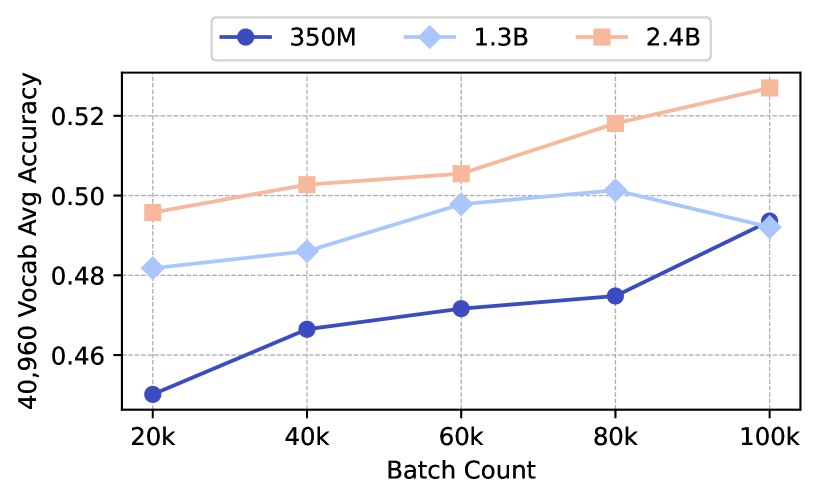<details> <summary>x7.png Details</summary>  ### Visual Description \n ## Line Chart: Model Accuracy vs. Batch Count ### Overview This image is a line chart comparing the performance of three different model sizes (350M, 1.3B, and 2.4B parameters) as a function of training batch count. The chart plots "40,960 Vocab Avg Accuracy" on the y-axis against "Batch Count" on the x-axis. The data suggests that larger models achieve higher accuracy and that accuracy generally improves with more training batches, though the rate of improvement varies. ### Components/Axes * **Chart Type:** Line chart with markers. * **X-Axis:** * **Label:** "Batch Count" * **Scale:** Linear scale with major tick marks at 20k, 40k, 60k, 80k, and 100k. * **Y-Axis:** * **Label:** "40,960 Vocab Avg Accuracy" * **Scale:** Linear scale ranging from approximately 0.45 to 0.53, with major tick marks at 0.46, 0.48, 0.50, and 0.52. * **Legend:** Positioned at the top center of the chart area. * **350M:** Dark blue line with solid circle markers. * **1.3B:** Light blue line with diamond markers. * **2.4B:** Orange line with square markers. * **Grid:** Light gray dashed grid lines are present for both major x and y-axis ticks. ### Detailed Analysis **Data Series and Trends:** 1. **350M Model (Dark Blue, Circles):** * **Trend:** Shows a consistent, moderately steep upward slope across all batch counts. * **Data Points (Approximate):** * 20k batches: ~0.450 * 40k batches: ~0.467 * 60k batches: ~0.472 * 80k batches: ~0.475 * 100k batches: ~0.493 2. **1.3B Model (Light Blue, Diamonds):** * **Trend:** Increases steadily from 20k to 80k batches, then shows a slight decrease or plateau between 80k and 100k batches. * **Data Points (Approximate):** * 20k batches: ~0.482 * 40k batches: ~0.486 * 60k batches: ~0.498 * 80k batches: ~0.501 * 100k batches: ~0.492 3. **2.4B Model (Orange, Squares):** * **Trend:** Exhibits the steepest and most consistent upward trend, maintaining the highest accuracy at every measured batch count. * **Data Points (Approximate):** * 20k batches: ~0.495 * 40k batches: ~0.503 * 60k batches: ~0.506 * 80k batches: ~0.518 * 100k batches: ~0.527 ### Key Observations * **Model Size Hierarchy:** There is a clear and consistent hierarchy in performance: 2.4B > 1.3B > 350M at all batch counts. * **Convergence at 100k:** The performance gap between the 350M and 1.3B models narrows significantly at 100k batches, with the 350M model nearly catching up to the 1.3B model's score. * **Diminishing Returns/Plateau:** The 1.3B model's performance appears to plateau or slightly regress after 80k batches, while the 2.4B model continues to improve strongly. * **Relative Improvement:** The 350M model shows the largest relative improvement from its starting point (~9.6% increase from 20k to 100k), while the 2.4B model shows the largest absolute gain (~0.032 points). ### Interpretation The chart demonstrates the principle of scaling laws in machine learning model training. Larger models (2.4B parameters) not only start at a higher accuracy but also continue to benefit more from extended training (increased batch count) compared to smaller models. The 1.3B model's plateau suggests it may have reached its capacity limit for this specific task and dataset at around 80k batches, or that further training without other adjustments (like learning rate decay) is not beneficial. The near-convergence of the 350M and 1.3B models at 100k batches is an interesting anomaly; it could indicate that the smaller model, given sufficient training time, can approach the performance of a moderately larger model on this specific metric, or it could be a point of measurement variance. Overall, the data strongly supports investing in both larger model sizes and longer training schedules for maximizing accuracy on this 40,960 vocabulary task. </details> Figure 7: Checkpoint accuracy values for PathPieceL with an initial vocabulary from BPE and a vocabulary size of 40,960, evaluated at 5 checkpoints. ## Appendix E Additional Analysis Here we additional details for results from § 6 that are just summarized in the text in the interest of space. ### E.1 Segmentation Tokenizers often use the segmentation strategy that is used in vocabulary construction. However, any vocabulary can also be used with PathPiece and with the greedy left-to-right segmentation methods. We find that BPE works quite well with greedy segmentation (overall rank 4, insignificantly different from the top rank), but not with the shortest-path segmentation of PathPieceL (13). 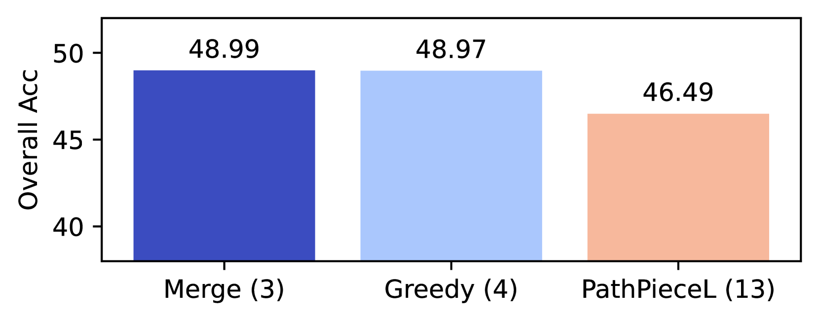<details> <summary>x8.png Details</summary>  ### Visual Description ## Bar Chart: Comparison of Overall Accuracy for Three Methods ### Overview The image displays a vertical bar chart comparing the "Overall Acc" (Overall Accuracy) of three distinct methods or algorithms. The chart is presented on a white background with a simple black border. The visual design uses color-coded bars to differentiate between the methods, with the exact accuracy value annotated above each bar. ### Components/Axes * **Y-Axis (Vertical):** * **Label:** "Overall Acc" * **Scale:** Linear scale ranging from 40 to 50. * **Major Tick Marks:** At 40, 45, and 50. * **X-Axis (Horizontal):** * **Categories:** Three distinct methods are listed. * **Labels (from left to right):** 1. "Merge (3)" 2. "Greedy (4)" 3. "PathPieceL (13)" * The numbers in parentheses (3, 4, 13) are part of the category labels but their specific meaning (e.g., parameter count, iteration number, variant ID) is not defined within the chart itself. * **Data Series (Bars):** * **Bar 1 (Left):** Dark blue bar corresponding to "Merge (3)". * **Bar 2 (Center):** Light blue bar corresponding to "Greedy (4)". * **Bar 3 (Right):** Peach/light orange bar corresponding to "PathPieceL (13)". * **Data Labels:** The precise numerical value of "Overall Acc" is displayed directly above each bar. ### Detailed Analysis The chart presents a direct comparison of a single performance metric across three items. 1. **Merge (3):** * **Color:** Dark blue. * **Reported Value:** 48.99 * **Visual Position:** The tallest bar, located on the far left. Its top aligns just below the 50 mark on the y-axis. 2. **Greedy (4):** * **Color:** Light blue. * **Reported Value:** 48.97 * **Visual Position:** The middle bar. Its height is visually almost identical to the "Merge (3)" bar, with a negligible difference of 0.02 in the reported value. 3. **PathPieceL (13):** * **Color:** Peach/light orange. * **Reported Value:** 46.49 * **Visual Position:** The shortest bar, located on the far right. It is noticeably shorter than the other two bars, sitting between the 45 and 50 marks on the y-axis. ### Key Observations * **Performance Cluster:** The "Merge (3)" and "Greedy (4)" methods form a high-performance cluster with nearly indistinguishable accuracy (48.99 vs. 48.97). The difference is within a hundredth of a percent. * **Performance Drop:** The "PathPieceL (13)" method shows a clear and significant drop in performance compared to the other two. Its accuracy is approximately 2.5 percentage points lower than the leading methods. * **Label Notation:** All category labels include a number in parentheses. The sequence (3, 4, 13) is not monotonic with performance, suggesting these numbers are not a direct ranking or a simple scaling factor for accuracy. ### Interpretation This chart likely comes from a technical or research context, comparing the effectiveness of different algorithms, models, or strategies on a common task where "Overall Accuracy" is the primary success metric. * **What the data suggests:** The "Merge" and "Greedy" approaches are essentially equivalent in terms of final accuracy for this specific evaluation. Choosing between them would depend on other factors not shown here, such as computational cost, speed, memory usage, or performance on secondary metrics. The "PathPieceL" method, while potentially offering other advantages (perhaps related to the number "13" in its label, such as using 13 components or steps), is less effective according to this accuracy measure. * **How elements relate:** The chart is designed for quick, at-a-glance comparison. The use of distinct colors and direct value labeling eliminates ambiguity in reading the results. The close pairing of the first two bars visually emphasizes their similarity, while the gap to the third bar highlights its inferior performance on this metric. * **Notable anomalies:** The primary anomaly is the minimal difference between the first two methods. In many experimental contexts, a difference of 0.02% would be considered statistically insignificant, suggesting these two methods may be functionally identical for this task. The meaning of the parenthetical numbers is the largest open question; without a caption or accompanying text, their significance is speculative (e.g., they could denote model size, number of training epochs, or a hyperparameter setting). </details> Figure 8: Segmentation of BPE. Pairwise $p$ -values between the pairs of runs are $p$ (3,4)=0.52, $p$ (3,13)=4.4e-5, $p$ (4,13)=8.8e-6. Unigram, on the other hand, seems to be more tightly tied to its default maximum likelihood segmentation (2), which was significantly better than both Greedy (7) and PathPieceL (17). 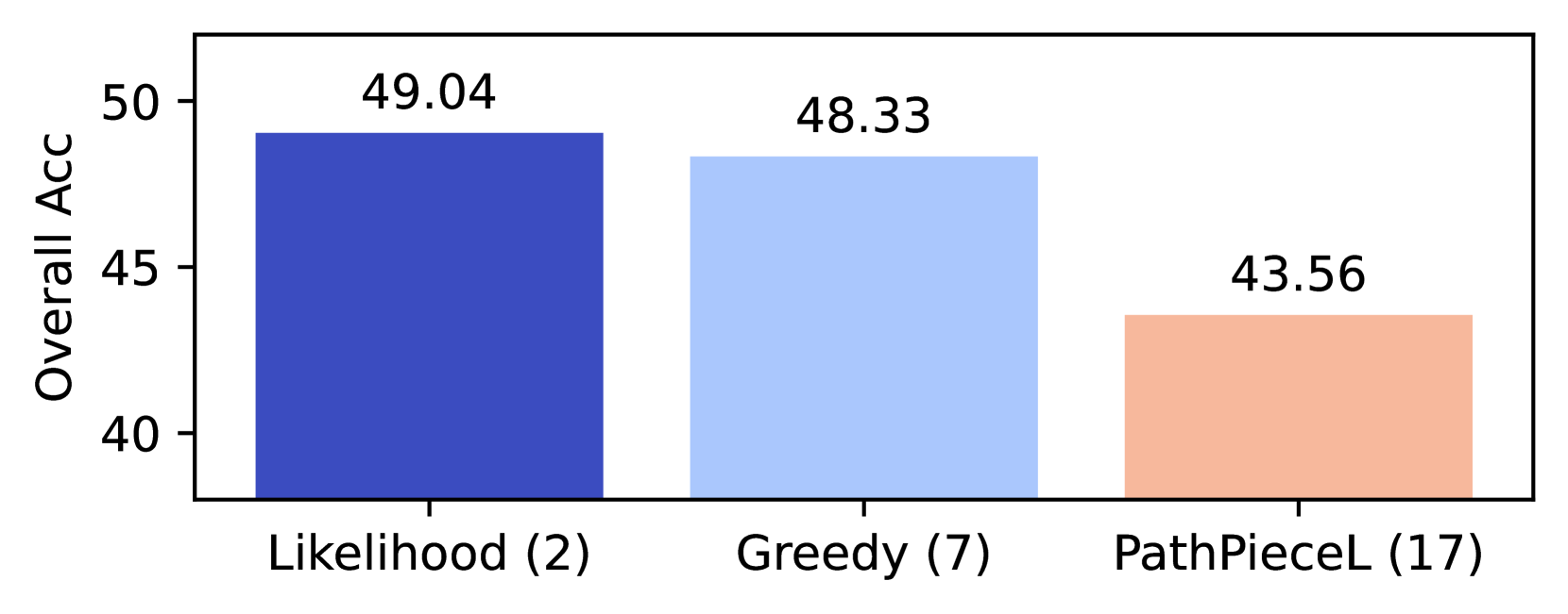<details> <summary>x9.png Details</summary>  ### Visual Description \n ## Bar Chart: Overall Accuracy Comparison of Three Methods ### Overview The image displays a vertical bar chart comparing the "Overall Acc" (Overall Accuracy) of three distinct methods or models. The chart presents a clear performance hierarchy, with one method achieving the highest accuracy and another showing a notably lower score. ### Components/Axes * **Y-Axis:** Labeled "Overall Acc". The scale ranges from 40 to 50, with major tick marks at intervals of 5 (40, 45, 50). * **X-Axis:** Contains three categorical labels, each corresponding to a bar. The labels are: 1. `Likelihood (2)` 2. `Greedy (7)` 3. `PathPieceL (17)` * **Data Series:** There are three bars, each a different color. The numerical value of each bar is displayed directly above it. * **Legend:** There is no separate legend box. The method names are provided as direct labels on the x-axis beneath each corresponding bar. ### Detailed Analysis The chart contains the following three data points, listed from left to right: 1. **Likelihood (2)** * **Position:** Leftmost bar. * **Color:** Dark blue. * **Value:** 49.04 * **Visual Trend:** This is the tallest bar, representing the highest accuracy. 2. **Greedy (7)** * **Position:** Center bar. * **Color:** Light blue. * **Value:** 48.33 * **Visual Trend:** This bar is slightly shorter than the "Likelihood (2)" bar, indicating a small decrease in accuracy. 3. **PathPieceL (17)** * **Position:** Rightmost bar. * **Color:** Peach/light orange. * **Value:** 43.56 * **Visual Trend:** This is the shortest bar by a significant margin, showing a substantial drop in accuracy compared to the other two methods. ### Key Observations * **Performance Hierarchy:** There is a clear ranking: `Likelihood (2)` > `Greedy (7)` > `PathPieceL (17)`. * **Magnitude of Difference:** The performance gap between the top two methods (`Likelihood` and `Greedy`) is relatively small (0.71 percentage points). The gap between the second and third method (`Greedy` and `PathPieceL`) is much larger (4.77 percentage points). * **Label Notation:** Each method name is followed by a number in parentheses (2, 7, 17). The chart does not provide a key to interpret these numbers; they may represent a version, a parameter setting, or another identifier specific to the context of the original document. ### Interpretation This chart demonstrates a comparative evaluation where the "Likelihood (2)" method achieves the best overall accuracy (49.04), closely followed by "Greedy (7)" (48.33). The "PathPieceL (17)" method performs significantly worse (43.56). The data suggests that for the task measured by "Overall Acc," the Likelihood-based approach is most effective, with the Greedy approach being a very close alternative. The PathPieceL method, under the configuration denoted by "(17)", is substantially less accurate. The numbers in parentheses are critical for reproducibility but are not explained within the visual itself. A viewer would need external context to understand if "(17)" indicates a more complex model, a different training regime, or another factor that might explain the performance drop. The chart effectively communicates that method choice has a major impact on outcome, with one option being clearly inferior in this specific metric. </details> Figure 9: Segmentation of Unigram. Pairwise $p$ -values between the pairs of runs are $p$ (2,7)=0.041, $p$ (2,17)=2.9e-06, $p$ (7,17)=2.9e-06 ### E.2 Digit Pre-tokenization We have two examples isolating Digit pre-tokenization, when a digit must always be its own token. Figure 10 shows Digit hurts for Sage with an $n$ -gram initial vocabulary, while Figure 11 shows no significant differences for PathPieceL, also with an $n$ -gram initial vocabulary. 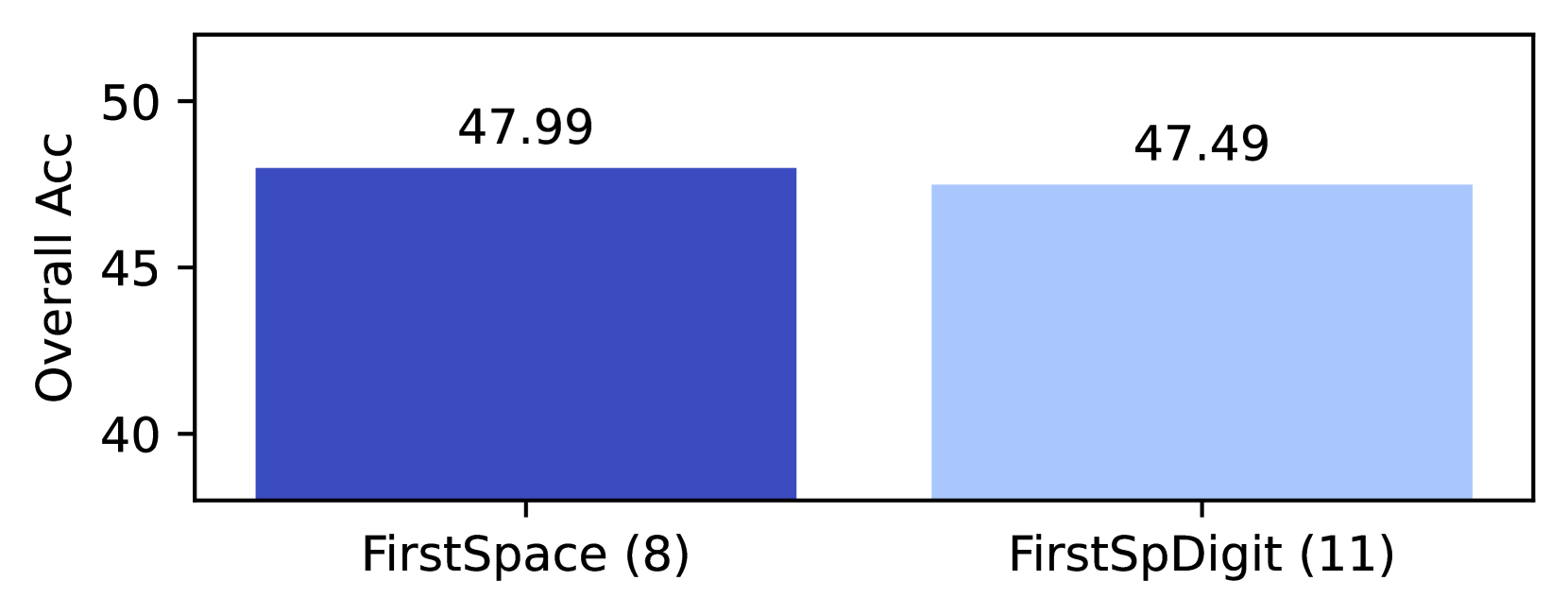<details> <summary>x10.png Details</summary>  ### Visual Description ## Bar Chart: Overall Accuracy Comparison ### Overview The image displays a simple bar chart comparing the "Overall Acc" (Overall Accuracy) of two distinct methods or conditions, labeled "FirstSpace (8)" and "FirstSpDigit (11)". The chart presents a direct, side-by-side comparison of a single performance metric. ### Components/Axes * **Chart Type:** Vertical bar chart. * **Y-Axis:** * **Label:** "Overall Acc" (presumably Overall Accuracy). * **Scale:** Linear scale with major tick marks and labels at 40, 45, and 50. The axis starts at a baseline of approximately 38 (inferred from bar height). * **X-Axis:** * **Categories:** Two categorical bars. * **Category 1 (Left Bar):** Labeled "FirstSpace (8)". * **Category 2 (Right Bar):** Labeled "FirstSpDigit (11)". * **Data Series & Legend:** * There is no separate legend box. The categories are identified solely by their x-axis labels. * **Bar 1 (Left):** Filled with a solid, dark blue color. Corresponds to "FirstSpace (8)". * **Bar 2 (Right):** Filled with a solid, light blue color. Corresponds to "FirstSpDigit (11)". * **Data Labels:** Each bar has its exact numerical value displayed centered above it. ### Detailed Analysis * **FirstSpace (8):** * **Visual Trend:** The dark blue bar is the taller of the two. * **Value:** 47.99 (displayed above the bar). * **Position:** Left side of the chart. * **FirstSpDigit (11):** * **Visual Trend:** The light blue bar is slightly shorter than the dark blue bar. * **Value:** 47.49 (displayed above the bar). * **Position:** Right side of the chart. * **Numerical Difference:** The accuracy for "FirstSpace (8)" is 0.50 percentage points higher than for "FirstSpDigit (11)". ### Key Observations 1. **Minimal Performance Gap:** The primary observation is the very small difference in overall accuracy between the two conditions. The values 47.99 and 47.49 are extremely close. 2. **High Baseline Accuracy:** Both methods achieve an accuracy score in the high 40s, suggesting a challenging task where perfect accuracy is not achieved. 3. **Label Semantics:** The labels contain parenthetical numbers: "(8)" and "(11)". These likely represent a parameter, sample size, or version number associated with each method, but their exact meaning is not defined within the chart itself. 4. **Visual Emphasis:** The use of contrasting blue shades (dark vs. light) clearly differentiates the two bars without implying a sequential relationship. ### Interpretation The chart demonstrates that the "FirstSpace" method, with the parameter or identifier (8), yields a marginally higher overall accuracy than the "FirstSpDigit" method with parameter (11). The difference of 0.50 is small and may not be statistically significant without additional context on variance or sample size. The data suggests that for the measured task, these two approaches are highly comparable in performance. The choice between them might therefore depend on other factors not shown here, such as computational cost, speed, or performance on specific sub-tasks. The parenthetical numbers hint at an underlying variable (e.g., model size, feature count, iteration number) that is being compared, but the chart alone does not reveal whether a higher or lower number is expected to correlate with accuracy. The investigation would require cross-referencing this result with the experimental setup to understand why the method labeled with (8) slightly outperforms the one with (11). </details> Figure 10: Pre-tokenization of Sage, $n$ -gram initial, $p$ =0.025. 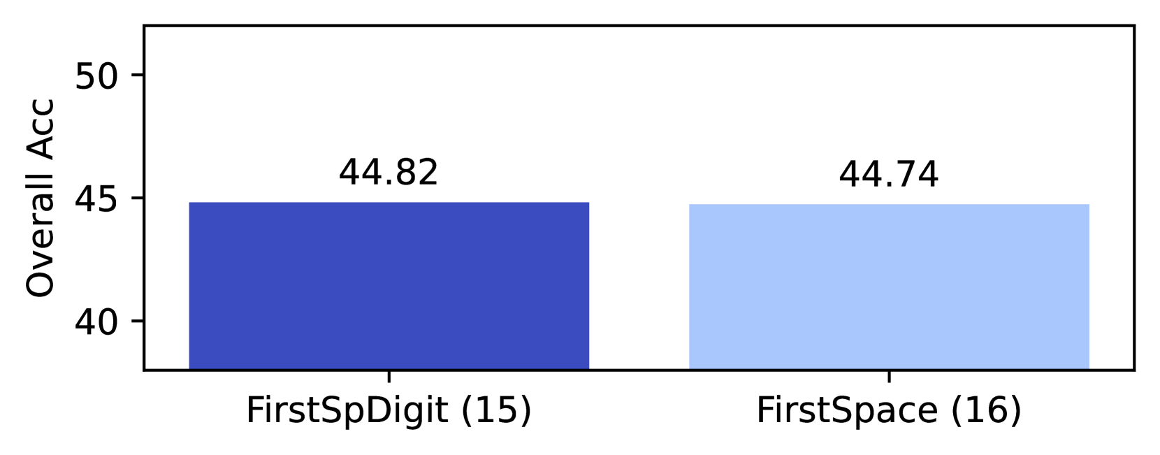<details> <summary>x11.png Details</summary>  ### Visual Description ## Bar Chart: Overall Accuracy Comparison ### Overview The image displays a simple vertical bar chart comparing the "Overall Acc" (Overall Accuracy) of two distinct categories or methods. The chart is presented on a white background with a black border. The visual design uses two shades of blue to differentiate the categories. ### Components/Axes * **Y-Axis (Vertical):** * **Title:** "Overall Acc" (presumably an abbreviation for Overall Accuracy). * **Scale:** Linear scale ranging from 40 to 50. * **Axis Markers/Ticks:** Labeled at intervals of 5: `40`, `45`, `50`. * **X-Axis (Horizontal):** * **Category Labels:** Two categories are listed below their respective bars. 1. `FirstSpDigit (15)` - Positioned below the left bar. 2. `FirstSpace (16)` - Positioned below the right bar. * The numbers in parentheses `(15)` and `(16)` are part of the category labels. Their meaning (e.g., sample size, version number) is not defined within the chart. * **Data Series (Bars):** * **Left Bar:** A solid, dark blue bar representing the category `FirstSpDigit (15)`. * **Right Bar:** A solid, light blue bar representing the category `FirstSpace (16)`. * **Data Labels:** Numerical values are displayed directly above each bar. * Above the left (dark blue) bar: `44.82` * Above the right (light blue) bar: `44.74` ### Detailed Analysis * **Value Extraction:** * The accuracy for `FirstSpDigit (15)` is **44.82**. * The accuracy for `FirstSpace (16)` is **44.74**. * **Trend Verification:** Visually, the two bars are nearly identical in height. The dark blue bar (`FirstSpDigit (15)`) is marginally taller than the light blue bar (`FirstSpace (16)`), corresponding to the slightly higher numerical value (44.82 vs. 44.74). * **Spatial Grounding:** The legend (category labels) is placed directly below the x-axis, aligned with each bar. The data values are centered above their respective bars. The y-axis is positioned on the left side of the chart. ### Key Observations 1. **Minimal Difference:** The primary observation is the extremely small difference in Overall Accuracy between the two categories. The delta is only **0.08** percentage points (44.82 - 44.74). 2. **High Similarity:** The performance, as measured by this metric, is virtually indistinguishable between `FirstSpDigit (15)` and `FirstSpace (16)`. 3. **Scale Context:** The y-axis starts at 40, not 0. This truncation visually emphasizes the small difference between the bars, making them appear more distinct than they would on a zero-based scale. ### Interpretation This chart presents a performance comparison between two entities, likely algorithms, models, or experimental conditions named `FirstSpDigit` and `FirstSpace`. The numbers in parentheses may denote a parameter, iteration, or sample size. The data suggests that, based on the "Overall Accuracy" metric, there is **no meaningful performance difference** between the two. The 0.08-point advantage for `FirstSpDigit (15)` is likely statistically insignificant and within any reasonable margin of error for such a measurement. The choice of a truncated y-axis (starting at 40) is a common visualization technique to highlight small differences. However, it also risks overstating the practical significance of the difference. A viewer must consciously note the scale to understand that both methods perform at nearly the same level, just below 45% accuracy. **Conclusion:** The chart demonstrates parity in performance. The key takeaway is the similarity, not the slight difference. Any decision between `FirstSpDigit (15)` and `FirstSpace (16)` would need to be based on factors other than this Overall Accuracy score, such as computational cost, speed, performance on specific sub-tasks, or other metrics not shown here. </details> Figure 11: Pre-tokenization of PathPieceL $n$ -gram, $p$ =0.54. With the exception of mathqa, none of our downstream tasks were particularly mathematical in nature. It is likely this makes it hard to make a definitive judgement on Digit with our experiments. ### E.3 Vocabulary Construction Figure 12 gives a Venn diagram of the overlap in vocabularies between Unigram, PathPieceL, and SaGe, when both PathPieceL and SaGe were constructed from a large initial vocabulary of size 262,144 from Unigram. As with Figure 5, we see that PathPiece is more similar to Unigram, while SaGe chose more distinct tokens. 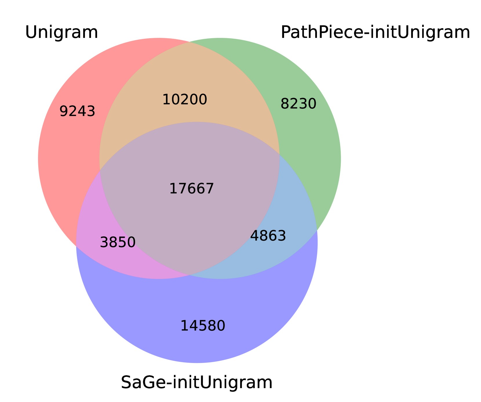<details> <summary>x12.png Details</summary>  ### Visual Description \n ## Venn Diagram: Overlap of Unigram Initialization Methods ### Overview This image is a three-set Venn diagram illustrating the numerical overlap and unique counts among three different unigram initialization methods or datasets: "Unigram," "PathPiece-initUnigram," and "SaGe-initUnigram." The diagram quantifies how many items (likely tokens, subwords, or data points) are shared between or unique to each method. ### Components/Axes * **Sets (Circles):** * **Top-Left Circle (Red/Pink):** Labeled "Unigram". * **Top-Right Circle (Green):** Labeled "PathPiece-initUnigram". * **Bottom Circle (Blue/Purple):** Labeled "SaGe-initUnigram". * **Regions & Values:** The diagram is divided into seven distinct regions, each containing a numerical count representing the cardinality of that specific intersection or unique set. * **Legend:** The labels for each circle serve as the legend, positioned adjacent to their respective circles. ### Detailed Analysis The diagram provides exact counts for all possible intersections of the three sets. The values are placed as follows: 1. **Unique to Unigram (Red/Pink region, top-left):** 9,243 2. **Unique to PathPiece-initUnigram (Green region, top-right):** 8,230 3. **Unique to SaGe-initUnigram (Blue/Purple region, bottom):** 14,580 4. **Shared by Unigram & PathPiece-initUnigram only (Orange/Tan region, top-center overlap):** 10,200 5. **Shared by Unigram & SaGe-initUnigram only (Pink/Purple region, left-center overlap):** 3,850 6. **Shared by PathPiece-initUnigram & SaGe-initUnigram only (Light Blue region, right-center overlap):** 4,863 7. **Shared by all three methods (Central Grey/Purple region):** 17,667 ### Key Observations * **Largest Unique Set:** The "SaGe-initUnigram" method has the highest number of unique items (14,580), significantly more than the other two. * **Largest Overlap:** The intersection of all three methods (17,667) is the single largest region in the diagram, indicating a substantial common core. * **Smallest Overlap:** The pairwise overlap between "Unigram" and "SaGe-initUnigram" (3,850) is the smallest intersection. * **Pairwise Comparisons:** The overlap between "Unigram" and "PathPiece-initUnigram" (10,200) is more than double the overlap between "Unigram" and "SaGe-initUnigram" (3,850). ### Interpretation This Venn diagram is a technical comparison of vocabulary or token sets resulting from different initialization strategies for a unigram language model, likely in the context of subword tokenization (e.g., for NLP models like SentencePiece). * **What the data suggests:** The three methods produce largely different sets, but with a very significant common core (17,667 items). "SaGe-initUnigram" appears to be the most distinct, generating the largest number of unique tokens not found in the other methods. "PathPiece-initUnigram" and "Unigram" share a larger common subset with each other than either does with "SaGe-initUnigram." * **How elements relate:** The diagram visually argues that while there is a foundational vocabulary agreed upon by all methods, the initialization technique ("PathPiece" vs. "SaGe") substantially influences the final token set, leading to unique specializations. The size of the unique sets suggests these methods might capture different linguistic features or handle rare words differently. * **Notable implications:** For a practitioner, this indicates that the choice of initialization method is not trivial. It will directly impact the model's vocabulary, potentially affecting its performance on specific tasks or domains. The large unique set for "SaGe-initUnigram" might imply it is more aggressive or specialized in its token creation. The substantial three-way overlap represents a stable, consensus vocabulary. </details> Figure 12: Venn diagrams comparing 40,960 token vocabularies of Unigram, PathPieceL and SaGe, where the latter two were both trained from a initial Unigram vocabulary of size 262,144 ### E.4 PathPiece tie breaking The difference in tie breaking between choosing the longest token with PathPieceL versus choosing randomly with PathPieceR turns out not to be significant, as seen in in Figure 13. 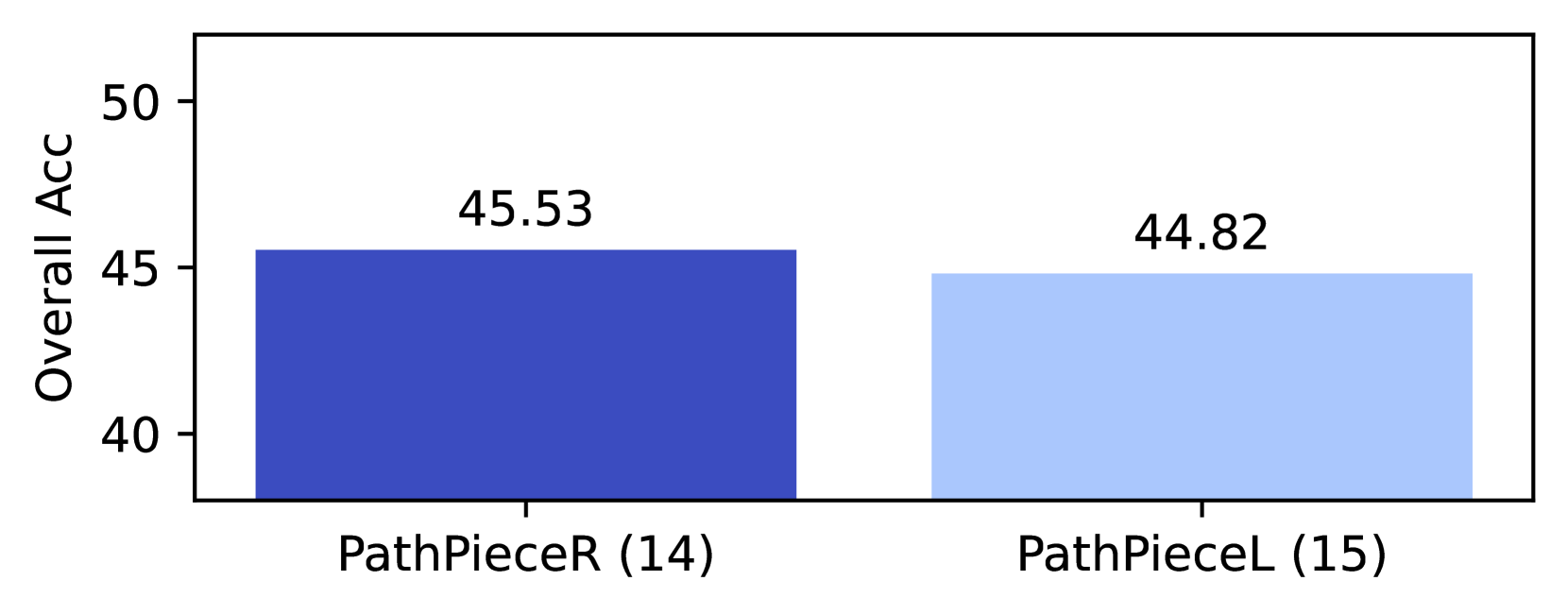<details> <summary>x13.png Details</summary>  ### Visual Description ## Comparative Bar Chart: Overall Accuracy Comparison ### Overview The image displays a simple vertical bar chart comparing the "Overall Acc" (Overall Accuracy) of two distinct items or methods, labeled "PathPieceR (14)" and "PathPieceL (15)". The chart presents a direct, side-by-side comparison of a single performance metric. ### Components/Axes * **Y-Axis (Vertical):** * **Label:** "Overall Acc" * **Scale:** Linear scale ranging from 40 to 50, with major tick marks at 40, 45, and 50. * **X-Axis (Horizontal):** * **Categories:** Two categorical bars. * **Labels (from left to right):** 1. "PathPieceR (14)" 2. "PathPieceL (15)" * **Legend:** Not present. The two bars are distinguished solely by their position and color. * **Data Labels:** Numerical values are displayed directly above each bar. ### Detailed Analysis 1. **Bar 1 (Left):** * **Category:** PathPieceR (14) * **Color:** Dark blue. * **Position:** Centered above the left x-axis label. * **Reported Value:** 45.53 * **Visual Height:** The top of the bar aligns slightly above the 45 mark on the y-axis, consistent with the labeled value. 2. **Bar 2 (Right):** * **Category:** PathPieceL (15) * **Color:** Light blue. * **Position:** Centered above the right x-axis label. * **Reported Value:** 44.82 * **Visual Height:** The top of the bar aligns just below the 45 mark on the y-axis, consistent with the labeled value. ### Key Observations * The performance difference between the two items is small, approximately 0.71 percentage points (45.53 - 44.82). * "PathPieceR (14)" demonstrates a marginally higher Overall Accuracy than "PathPieceL (15)". * Both values are clustered in the mid-40s range, indicating similar performance levels on this metric. * The chart uses a truncated y-axis (starting at 40, not 0), which visually emphasizes the small difference between the two bars. ### Interpretation This chart provides a focused comparison of a single accuracy metric between two entities, likely different models, algorithms, or experimental conditions denoted as "PathPieceR" and "PathPieceL" with associated identifiers (14) and (15). The data suggests that under the conditions measured, the "PathPieceR (14)" configuration achieves a slightly superior overall accuracy. However, the difference is less than one percentage point, which may or may not be statistically or practically significant depending on the broader context of the evaluation (e.g., sample size, variance, baseline performance). The primary takeaway is one of relative parity with a slight edge to PathPieceR. The chart is designed for quick, at-a-glance comparison rather than conveying complex trends, as it presents a single data point for each category. The use of distinct colors (dark vs. light blue) and clear numerical labels ensures the comparison is unambiguous. </details> Figure 13: Tiebreaking PathPieceL vs PathPieceR with $n$ -gram, $p$ =0.067. ## Appendix F RandTrain None of our experiments completely isolate the effect of the vocabulary construction step. We created a new baseline random vocabulary construction approach, RandTrain, in an attempt to do so. It is meant to work with a top-down method like SaGe or PathPieceL, and uses the same initial vocabulary, pre-tokenization, and segmentation as either of those, with a simple vocabulary construction algorithm. We compute a count for each token in the vocabulary. For the top $n$ -gram initial vocabulary it is simply the $n$ -gram count from the training corpus. For a BPE initial vocabulary we tokenized the training corpus with BPE and the large initial vocabulary, and then use the occurrence counts of each token. We normalize these counts into target selection probabilities $p_k$ for token $t_k$ . The RandTrain vocabulary construction process is simply to randomly sample our desired vocabulary size $m$ of tokens from the initial vocabulary, proportionally to $p_k$ , without replacement. Sampling without replacement is necessary to avoid have duplicate words in the vocabulary. Interestingly, this is not possible if there are any $p_k>1/m$ , which are termed infeasible or overweight items Efraimidis (2010). The intuition behind this is when selecting $m$ items without replacement, it is not possible to select a given item more than once. So even if an item is always selected in a sample, the selection probability will be $p_k=1/m$ . We sampled without replacement using the A-ES Algorithm described in Efraimidis (2010). A significant number the most common tokens in the vocabulary were infeasible and hence were unable to reach their target $p_k$ . A token with a higher $p_k$ is more likely to be sampled than a token with a lower one, but they may significantly differ from their target $p_k$ . We build 6 RandTrain models with 3 different types of pre-tokenization, and with Greedy segmentation to compare to SaGe, and PathPieceL segmentation to compare to PathPieceL. We only used a single vocabulary size of 40,960, so $p$ -values are only computed on the 10 task accuracies, rather than the 30 used elsewhere. Task level accuracies are given in Table 6 and Table 7 in Appendix G. Before comparing RandTrain to SaGe and PathPieceL, we will compare our RandTrain runs to each other, with different segmentation approaches. In Figure 14 and Figure 16 we have pairs of RandTrain runs that only vary by the segmentation method. 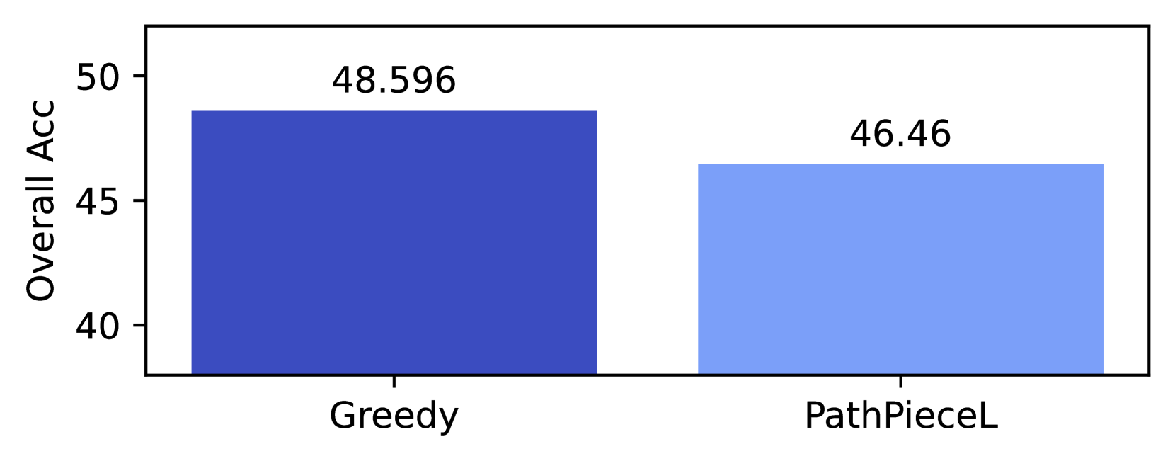<details> <summary>x14.png Details</summary>  ### Visual Description ## Bar Chart: Overall Accuracy Comparison ### Overview The image displays a simple vertical bar chart comparing the "Overall Acc" (Overall Accuracy) of two distinct methods or models, labeled "Greedy" and "PathPieceL". The chart presents a direct performance comparison, with the "Greedy" method achieving a higher accuracy score. ### Components/Axes * **Chart Type:** Vertical Bar Chart. * **Y-Axis:** * **Label:** "Overall Acc" (presumably Overall Accuracy). * **Scale:** Linear scale with major tick marks at 40, 45, and 50. The axis is truncated, starting at 40 rather than 0. * **X-Axis:** * **Categories:** Two categorical bars. * **Labels (from left to right):** "Greedy" and "PathPieceL". * **Data Series & Values:** * **Greedy:** Represented by a dark blue bar. The exact value, annotated above the bar, is **48.596**. * **PathPieceL:** Represented by a light blue bar. The exact value, annotated above the bar, is **46.46**. * **Legend:** Not present. Category identification is provided by direct labels under each bar. * **Spatial Layout:** The "Greedy" bar is positioned on the left side of the chart area, and the "PathPieceL" bar is on the right. The y-axis label is rotated 90 degrees and placed to the left of the axis. ### Detailed Analysis * **Data Point Extraction:** * **Greedy:** Accuracy = 48.596 * **PathPieceL:** Accuracy = 46.46 * **Trend/Comparison:** The "Greedy" bar is visually taller than the "PathPieceL" bar, indicating a higher accuracy value. The numerical difference is 48.596 - 46.46 = **2.136** percentage points. * **Visual Representation:** The y-axis range (40 to ~50) visually amplifies the difference between the two bars. The "Greedy" bar extends from the baseline (40) to just below the 50 mark, while the "PathPieceL" bar extends to a point slightly above the 45 mark. ### Key Observations 1. **Performance Hierarchy:** The "Greedy" method demonstrates superior performance over "PathPieceL" on the "Overall Acc" metric. 2. **Truncated Axis:** The y-axis starts at 40, not 0. This is a common practice to highlight differences in data points that are close in value, but it can visually exaggerate the relative difference if not noted by the viewer. 3. **Precision of Annotation:** The values are provided with high precision (three decimal places for Greedy, two for PathPieceL), suggesting these are calculated metrics from an experiment or evaluation. 4. **Simplicity:** The chart is minimal, containing only the essential elements needed for the comparison: two bars, their labels, and their exact values. ### Interpretation This chart provides a clear, quantitative snapshot comparing two approaches. The data suggests that, under the conditions measured by "Overall Acc," the "Greedy" approach is more effective than "PathPieceL" by a margin of approximately 2.1 percentage points. The choice of a truncated y-axis is a deliberate design decision to make this ~2-point difference more visually apparent. While this aids in quick visual comparison, a technical reader should note the absolute scale to properly contextualize the magnitude of the improvement. The high precision of the reported values implies this is likely a result from a controlled computational experiment, such as evaluating machine learning models or algorithmic performance on a specific task. The absence of error bars or confidence intervals means we cannot assess the statistical significance of the observed difference from this chart alone. 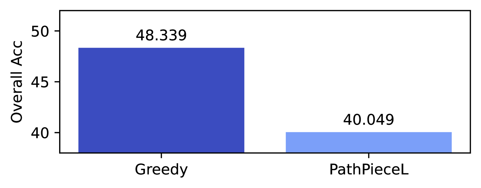</details> Figure 14: Comparison of Greedy and PathPieceL segmentation, with RandTrain vocabulary construction, BPE initial vocab, and FirstSpace pre-tokenization, $p$ =0.0273 <details> <summary>x15.png Details</summary>  ### Visual Description ## Bar Chart: Overall Accuracy Comparison ### Overview The image is a simple vertical bar chart comparing the "Overall Acc" (Overall Accuracy) of two distinct methods or models, labeled "Greedy" and "PathPieceL". The chart presents a single performance metric for each. ### Components/Axes * **Y-Axis (Vertical):** * **Label:** "Overall Acc" * **Scale:** Linear scale with major tick marks and numerical labels at 40, 45, and 50. * **Range:** The visible axis spans from slightly below 40 to slightly above 50. * **X-Axis (Horizontal):** * **Categories:** Two categorical labels are present: 1. "Greedy" (positioned on the left) 2. "PathPieceL" (positioned on the right) * **Data Series (Bars):** * **Bar 1 (Left):** Corresponds to "Greedy". It is a solid, dark blue bar. * **Bar 2 (Right):** Corresponds to "PathPieceL". It is a solid, light blue bar. * **Data Labels:** Each bar has its exact numerical value displayed directly above it. * Above "Greedy" bar: `48.339` * Above "PathPieceL" bar: `40.049` ### Detailed Analysis * **Greedy Method:** * **Visual Trend:** The dark blue bar is significantly taller than the light blue bar. * **Data Point:** The accuracy value is explicitly stated as **48.339**. * **Spatial Grounding:** The bar originates from the x-axis at the "Greedy" label and extends vertically to a height corresponding to approximately 48.3 on the y-axis scale. * **PathPieceL Method:** * **Visual Trend:** The light blue bar is shorter than the dark blue bar. * **Data Point:** The accuracy value is explicitly stated as **40.049**. * **Spatial Grounding:** The bar originates from the x-axis at the "PathPieceL" label and extends vertically to a height corresponding to approximately 40.0 on the y-axis scale. ### Key Observations 1. **Clear Performance Gap:** There is a substantial difference in overall accuracy between the two methods. The "Greedy" method outperforms "PathPieceL". 2. **Magnitude of Difference:** The numerical difference is `48.339 - 40.049 = 8.290` percentage points (assuming "Acc" is percentage-based). 3. **Visual Encoding:** The chart uses color (dark blue vs. light blue) and spatial separation (left vs. right) to distinguish the two categories. No separate legend is present, as the category labels are placed directly below their respective bars. ### Interpretation The data demonstrates that, for the given task and evaluation metric ("Overall Acc"), the "Greedy" approach is markedly more effective than the "PathPieceL" approach. The difference of over 8 percentage points is likely significant in most technical contexts, suggesting "Greedy" is the superior method based on this single metric. The chart's design is minimalist and direct, focusing the viewer's attention solely on the comparison of the two final accuracy scores. It does not provide information on variance, statistical significance, the nature of the task, or the underlying mechanisms of the methods. Therefore, while the chart clearly answers "which performed better?", it does not explain "why?" or "under what conditions?". To draw broader conclusions, one would need additional context about the experimental setup and results from other metrics. 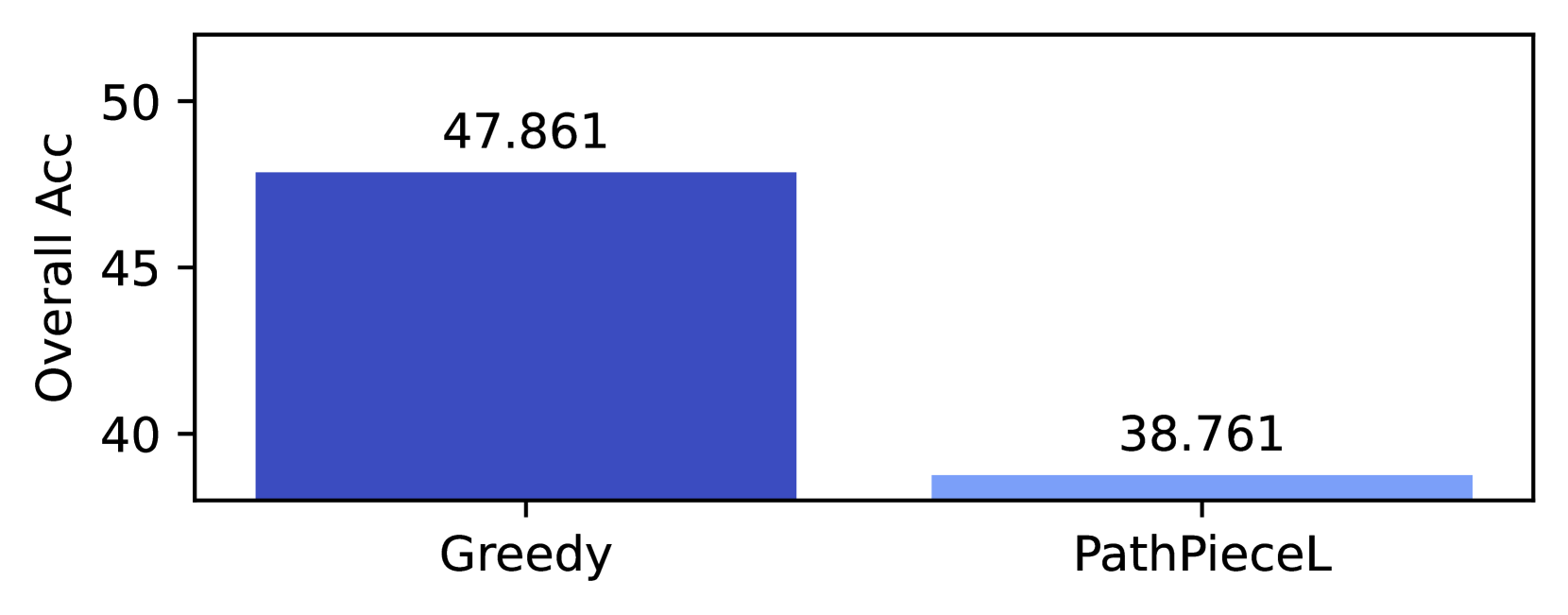</details> Figure 15: Comparison of Greedy and PathPieceL segmentation, with RandTrain vocabulary construction, $n$ -gram initial vocab, and FirstSpace pre-tokenization, $p$ =0.00195 <details> <summary>x16.png Details</summary>  ### Visual Description ## Bar Chart: Comparison of Overall Accuracy Between Two Methods ### Overview The image displays a simple vertical bar chart comparing the "Overall Acc" (Overall Accuracy) of two distinct methods or algorithms. The chart is presented on a white background with a black border. It contains two bars, each representing a single data point with its exact numerical value annotated above it. ### Components/Axes * **Chart Type:** Vertical Bar Chart. * **Y-Axis:** * **Label:** "Overall Acc" (presumably an abbreviation for Overall Accuracy). * **Scale:** Linear scale with major tick marks and numerical labels at 40, 45, and 50. * **Range:** The visible axis spans from slightly below 40 to slightly above 50. * **X-Axis:** * **Categories:** Two categorical labels are present below the bars: "Greedy" and "PathPieceL". * **Data Series & Legend:** There is no separate legend. The two bars are distinguished by color and their corresponding x-axis labels. * **Bar 1 (Left):** Labeled "Greedy". Colored in a solid, dark blue. * **Bar 2 (Right):** Labeled "PathPieceL". Colored in a solid, light blue. * **Data Labels:** The precise numerical value for each bar is displayed directly above it in black text. ### Detailed Analysis * **Data Point 1 - Greedy:** * **Position:** Left side of the chart. * **Color:** Dark blue. * **Value:** 47.861 (annotated above the bar). * **Visual Trend:** The bar extends vertically from the baseline (below 40) to a height corresponding to its value, clearly surpassing the 45 mark on the y-axis. * **Data Point 2 - PathPieceL:** * **Position:** Right side of the chart. * **Color:** Light blue. * **Value:** 38.761 (annotated above the bar). * **Visual Trend:** The bar is significantly shorter than the "Greedy" bar. Its top aligns just below the 40 mark on the y-axis. ### Key Observations 1. **Significant Performance Gap:** There is a substantial difference in Overall Accuracy between the two methods. The "Greedy" method (47.861) outperforms the "PathPieceL" method (38.761) by approximately **9.1 percentage points**. 2. **Visual Confirmation:** The dark blue "Greedy" bar is visually about 23% taller than the light blue "PathPieceL" bar, which is consistent with the numerical difference. 3. **Baseline Context:** Both values are presented on a scale starting near 40, which visually accentuates the difference between them. The "PathPieceL" value is below the lowest labeled tick mark (40). ### Interpretation This chart presents a direct, head-to-head comparison of two techniques, likely from a computational or machine learning context, based on a single performance metric: Overall Accuracy. * **What the data suggests:** The "Greedy" approach demonstrates markedly superior performance compared to "PathPieceL" for the task measured. The magnitude of the difference (over 9 points) is typically considered highly significant in fields where accuracy is a key metric. * **How elements relate:** The chart's design is minimalist, focusing the viewer's attention solely on the contrast between the two values. The use of different shades of blue groups the data as related (both are accuracy scores) while still differentiating the categories. The placement of exact values above the bars removes any ambiguity in reading the chart. * **Notable considerations:** The chart does not provide context for what "Greedy" or "PathPieceL" refer to, nor the specific task or dataset used. The y-axis label "Overall Acc" is an abbreviation; in a full technical document, this would be defined (e.g., "Overall Accuracy on the X Benchmark"). The choice to start the y-axis near 40 (a "truncated graph") emphasizes the difference between the two values, which is a common and acceptable practice when the focus is on comparing magnitudes rather than showing absolute zero. </details> Figure 16: Comparison of Greedy and PathPieceL segmentation, with RandTrain vocabulary construction, $n$ -gram initial vocab, and FirstSpaceDigit pre-tokenization, $p$ =0.00293 In line with Subsection E.1, Greedy performs significantly better than PathPieceL segmentation in all 3 cases. However, for the two cases with an $n$ -gram initial vocabulary the PathPieceL segmentation did extremely poorly. The RandTrain vocabulary construction, $n$ -gram initial vocabulary, and PathPieceL segmentation interact somehow to give accuracies well below any others. This makes the comparison of RandTrain to PathPieceL less informative. We can see in Figure 17 that PathPieceL is significantly better than RandTrain with a BPE initial vocabulary. However, the other two comparisons in Figure 18 are Figure 19 are not that meaningful. They are significantly better, but that is more about the weak baseline of RandTrain with PathPieceL segmentation than anything positive about PathPieceL. 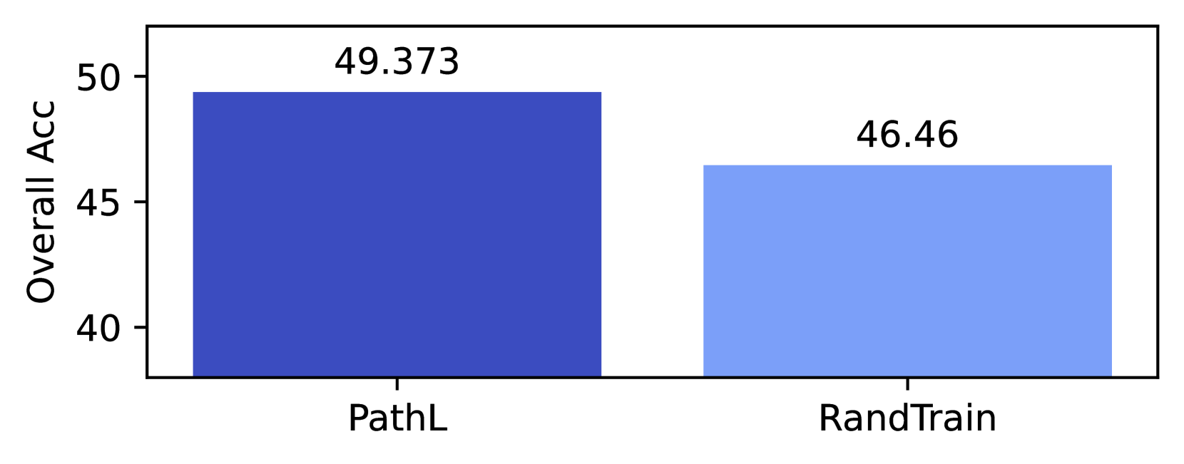<details> <summary>x17.png Details</summary>  ### Visual Description \n ## Bar Chart: Overall Accuracy Comparison ### Overview The image displays a simple vertical bar chart comparing the "Overall Acc" (Overall Accuracy) of two distinct methods or models, labeled "PathL" and "RandTrain". The chart presents a direct performance comparison, with numerical values annotated above each bar. ### Components/Axes * **Chart Type:** Vertical Bar Chart. * **Y-Axis:** * **Label:** "Overall Acc" (written vertically along the left side). * **Scale:** Linear scale ranging from 40 to 50. * **Major Ticks:** Marked at intervals of 5 (40, 45, 50). * **X-Axis:** * **Categories:** Two categorical bars. * **Category Labels:** "PathL" (left bar) and "RandTrain" (right bar). * **Data Series & Values:** * **PathL:** Represented by a dark blue bar. The exact value annotated above the bar is **49.373**. * **RandTrain:** Represented by a light blue bar. The exact value annotated above the bar is **46.46**. * **Legend:** No separate legend is present. The categories are identified solely by their x-axis labels and distinct bar colors. * **Title:** No chart title is visible in the image. ### Detailed Analysis * **Spatial Grounding & Color Confirmation:** The left bar, positioned above the "PathL" label, is colored dark blue and corresponds to the value 49.373. The right bar, positioned above the "RandTrain" label, is colored light blue and corresponds to the value 46.46. * **Trend Verification:** The chart shows a direct comparison, not a time-series trend. The visual trend is that the "PathL" bar is taller than the "RandTrain" bar, indicating a higher value. * **Data Points:** * PathL: 49.373 * RandTrain: 46.46 * **Derived Difference:** The absolute difference in Overall Accuracy between PathL and RandTrain is approximately **2.913** (49.373 - 46.46). ### Key Observations 1. **Performance Gap:** The "PathL" method demonstrates a higher Overall Accuracy than the "RandTrain" method. 2. **Precision of Reporting:** The values are reported to two and three decimal places (46.46 and 49.373, respectively), suggesting the measurements or calculations were performed with high precision. 3. **Scale Focus:** The y-axis starts at 40, not 0. This visual choice emphasizes the difference between the two values but does not distort the relative comparison since both bars are measured against the same baseline. ### Interpretation The data suggests that the "PathL" approach is more effective, as measured by "Overall Acc," than the "RandTrain" approach for the given task or dataset. The difference of nearly 3 percentage points is likely significant in a machine learning or statistical modeling context, where small improvements in accuracy can be meaningful. Without additional context (e.g., what "PathL" and "RandTrain" specifically refer to, the nature of the task, or the dataset), the interpretation is limited to this relative performance comparison. "RandTrain" may imply a randomized training baseline, while "PathL" could refer to a method incorporating path-based learning or logic. The chart's primary message is the superiority of PathL over this particular baseline in terms of the reported accuracy metric. 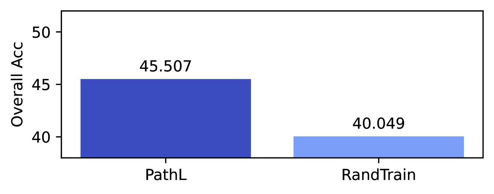</details> Figure 17: Comparison of PathPieceL and RandTrain, with BPE initial vocab, and FirstSpace pre-tokenization, $p$ =0.0137 <details> <summary>x18.png Details</summary>  ### Visual Description ## Bar Chart: Comparison of Overall Accuracy for PathL and RandTrain ### Overview The image is a simple vertical bar chart comparing the "Overall Acc" (Overall Accuracy) of two distinct methods or models, labeled "PathL" and "RandTrain". The chart presents a single performance metric for each. ### Components/Axes * **Y-Axis (Vertical):** * **Label:** "Overall Acc" * **Scale:** Linear scale ranging from 40 to 50, with major tick marks at 40, 45, and 50. * **X-Axis (Horizontal):** * **Categories:** Two categorical bars. * **Labels:** "PathL" (left bar) and "RandTrain" (right bar). * **Legend:** There is no separate legend; the categories are labeled directly on the x-axis. * **Data Labels:** The exact numerical value of each bar is displayed directly above it. ### Detailed Analysis * **Data Series 1: PathL** * **Position:** Left side of the chart. * **Color:** Dark blue. * **Value:** 45.507 * **Visual Trend:** This is the taller of the two bars, indicating a higher accuracy value. * **Data Series 2: RandTrain** * **Position:** Right side of the chart. * **Color:** Light blue. * **Value:** 40.049 * **Visual Trend:** This is the shorter bar, indicating a lower accuracy value. ### Key Observations 1. **Performance Gap:** The "PathL" method demonstrates a higher overall accuracy than "RandTrain". The difference is approximately 5.458 percentage points (45.507 - 40.049). 2. **Y-Axis Truncation:** The y-axis starts at 40, not 0. This visual choice amplifies the perceived difference between the two bars. While the numerical difference is clear, the visual height ratio of the bars does not represent the ratio of their values (45.507 / 40.049 ≈ 1.14, but the visual height ratio is much larger). 3. **Precision:** The accuracy values are reported to three decimal places, suggesting a precise measurement or calculation. ### Interpretation The chart provides a direct, quantitative comparison between two approaches, likely in a machine learning or experimental context. "PathL" is shown to be the superior method according to the "Overall Acc" metric. The choice to label the y-axis "Overall Acc" implies this is an aggregate performance score, possibly across multiple classes, tasks, or test sets. The names "PathL" and "RandTrain" suggest a comparison between a structured or path-based learning method ("PathL") and a method involving randomization in training ("RandTrain"). The data clearly supports the conclusion that the structured approach yields better overall accuracy in this specific evaluation. The absence of a chart title, gridlines, or error bars means the viewer must rely solely on the provided labels and values. The clean, minimal design focuses attention entirely on the two comparative values. 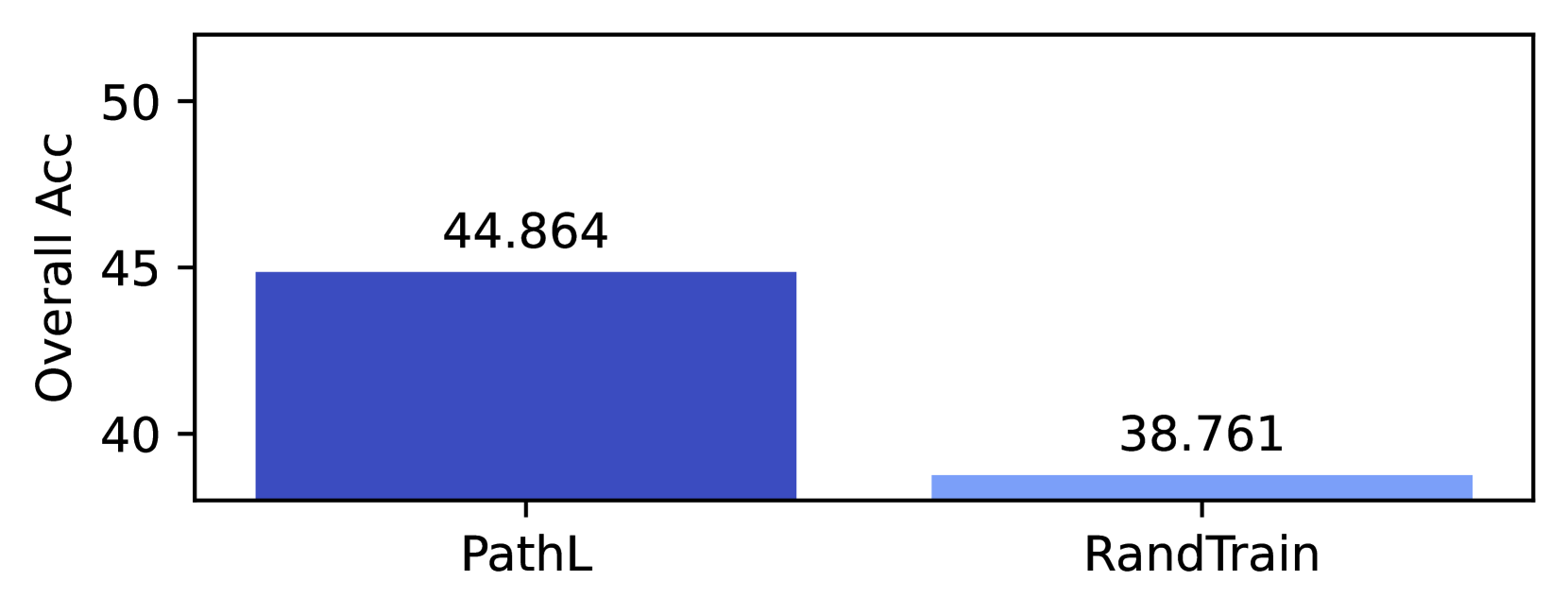</details> Figure 18: Comparison of PathPieceL and RandTrain, with $n$ -gram initial vocab, and FirstSpace pre-tokenization, $p$ =9.77e-4 <details> <summary>x19.png Details</summary>  ### Visual Description ## Bar Chart: Overall Accuracy Comparison ### Overview The image displays a simple vertical bar chart comparing the "Overall Acc" (Overall Accuracy) of two distinct methods or models, labeled "PathL" and "RandTrain." The chart is presented on a white background with a black border. There is no main title for the chart. ### Components/Axes * **Y-Axis (Vertical):** * **Label:** "Overall Acc" * **Scale:** Linear scale ranging from 40 to 50. * **Tick Marks:** Major ticks are present at 40, 45, and 50. * **X-Axis (Horizontal):** * **Categories:** Two categorical bars are present. * **Labels:** The left bar is labeled "PathL." The right bar is labeled "RandTrain." * **Data Series & Legend:** * There is no explicit legend. The two data series are distinguished solely by their x-axis labels and bar color. * **Bar 1 (PathL):** A solid, dark blue bar. * **Bar 2 (RandTrain):** A solid, light blue bar. * **Data Labels:** Numerical values are displayed directly above each bar. ### Detailed Analysis * **PathL Bar:** * **Position:** Left side of the chart. * **Color:** Dark blue. * **Height:** The bar extends from the baseline (below 40) to a point just below the 45 tick mark on the y-axis. * **Value:** The data label above the bar reads **44.864**. * **RandTrain Bar:** * **Position:** Right side of the chart. * **Color:** Light blue. * **Height:** The bar is significantly shorter, extending from the baseline to a point just below the 40 tick mark. * **Value:** The data label above the bar reads **38.761**. ### Key Observations 1. **Significant Performance Gap:** There is a clear and substantial difference in Overall Accuracy between the two methods. PathL outperforms RandTrain by a margin of approximately 6.103 percentage points (44.864 - 38.761). 2. **Visual Confirmation:** The trend is visually unambiguous. The dark blue bar (PathL) is markedly taller than the light blue bar (RandTrain), corroborating the numerical values. 3. **Scale Context:** The y-axis is truncated, starting at 40 instead of 0. This visual choice emphasizes the difference between the two values but does not alter the factual data presented. ### Interpretation The chart presents a direct, quantitative comparison between two approaches, "PathL" and "RandTrain," on a metric called "Overall Acc." The data strongly suggests that the PathL method achieves a meaningfully higher level of overall accuracy than the RandTrain method in the evaluated context. The absence of a chart title, units for "Acc" (though likely percentage), or any description of the experimental setup limits a full interpretation. However, the core message is clear: PathL is the superior performer according to this specific metric. The use of distinct colors (dark vs. light blue) effectively separates the two categories for quick visual comparison. The presentation is minimalist, focusing solely on the final accuracy values without showing variance, error bars, or other statistical context. </details> Figure 19: Comparison of PathPieceL and RandTrain, with $n$ -gram initial vocab, and FirstSpaceDigits pre-tokenization, $p$ =0.00977 The remaining comparison between SaGe and RandTrain is more interesting. In Figure 20 and Figure 21 SaGe was not significantly better than RandTrain, with a $p$ -value of 0.0645. 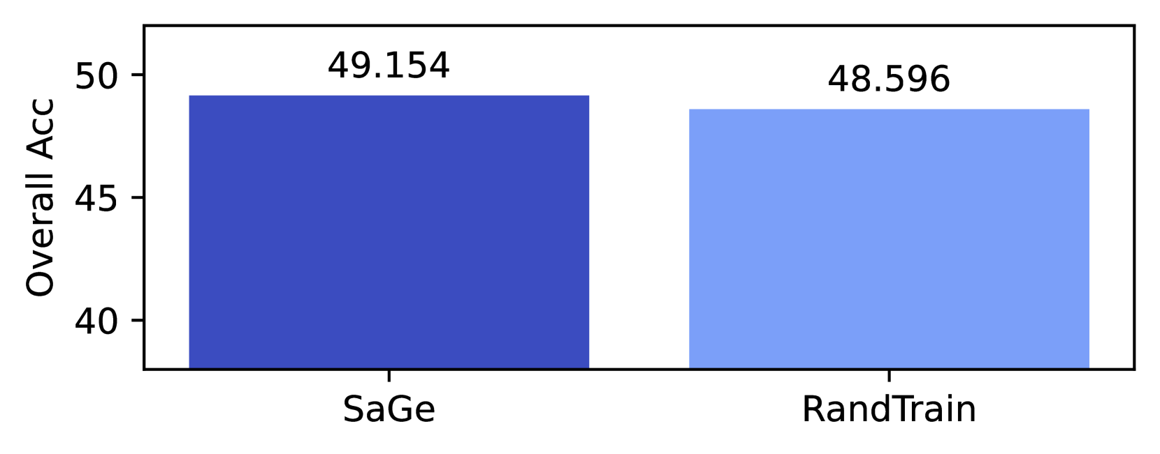<details> <summary>x20.png Details</summary>  ### Visual Description ## Bar Chart: Overall Accuracy Comparison ### Overview The image displays a simple vertical bar chart comparing the "Overall Acc" (Overall Accuracy) of two distinct methods or models: "SaGe" and "RandTrain". The chart presents a direct, side-by-side comparison of a single performance metric. ### Components/Axes * **Y-Axis (Vertical):** * **Label:** "Overall Acc" * **Scale:** Linear scale ranging from 40 to 50. * **Tick Marks:** Major ticks are present at 40, 45, and 50. * **X-Axis (Horizontal):** * **Categories:** Two categorical bars are present. * **Labels (from left to right):** "SaGe" and "RandTrain". * **Data Series & Legend:** * There is no separate legend box. The categories are identified by the labels directly beneath each bar. * **Bar 1 (Left):** Labeled "SaGe". Colored in a dark, saturated blue. * **Bar 2 (Right):** Labeled "RandTrain". Colored in a lighter, less saturated blue. * **Data Labels:** * Numerical values are displayed directly above each bar. * Value above "SaGe" bar: **49.154** * Value above "RandTrain" bar: **48.596** ### Detailed Analysis * **SaGe Performance:** The bar representing "SaGe" reaches a height corresponding to an Overall Accuracy of **49.154**. This is the higher of the two values presented. * **RandTrain Performance:** The bar representing "RandTrain" reaches a height corresponding to an Overall Accuracy of **48.596**. * **Comparison:** The difference in Overall Accuracy between the two methods is **0.558** (49.154 - 48.596). Visually, the bars are very close in height, indicating a small performance gap. ### Key Observations 1. **Close Performance:** The primary observation is the proximity of the two accuracy scores. The visual difference in bar height is minimal, reflecting the small numerical difference of approximately 0.56 percentage points. 2. **Metric Focus:** The chart isolates and compares a single, high-level metric ("Overall Acc"), providing no insight into other potential performance dimensions like precision, recall, or computational cost. 3. **Visual Encoding:** The chart uses color (dark blue vs. light blue) and spatial separation (left vs. right) to distinguish the two categories. The direct labeling below each bar and the value labels above them make the chart self-explanatory without a separate legend. ### Interpretation This chart presents a performance benchmark between two entities, likely machine learning models or training methodologies named "SaGe" and "RandTrain". The data suggests that **SaGe achieves a marginally higher Overall Accuracy than RandTrain**. The key takeaway is not a dramatic superiority but a slight edge. In a technical context, this small difference could be significant depending on the application's sensitivity to accuracy improvements. It prompts further investigation: * Is this difference statistically significant? * What are the trade-offs? Does SaGe require more data, computation, or time to achieve this gain? * How does this "Overall Acc" break down across different classes or subsets of the data? The chart effectively communicates that, on this specific aggregate metric, SaGe is the top performer, but the margin is narrow enough that other factors (efficiency, robustness, fairness) would be critical in deciding which method to employ. </details> Figure 20: Comparison of SaGe and RandTrain, with BPE initial vocab, and FirstSpace pre-tokenization, $p$ =0.0645 The cases is even worse for the two $n$ -gram initial vocabulary cases. In Figure 21 the $p$ -value was a 0.688, and in Figure 22 RandTrain was actually better, although not significantly. 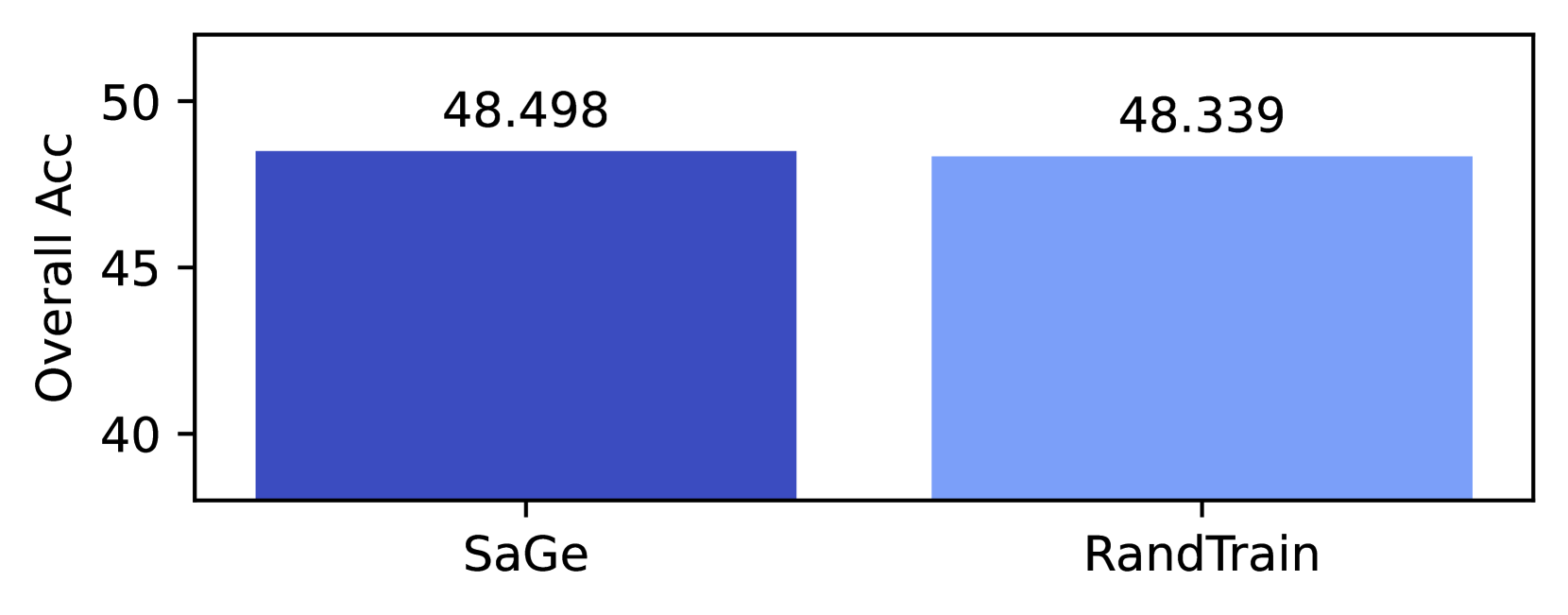<details> <summary>x21.png Details</summary>  ### Visual Description \n ## Bar Chart: Comparison of Overall Accuracy: SaGe vs. RandTrain ### Overview The image is a simple bar chart comparing the "Overall Acc" (Overall Accuracy) of two distinct methods or models, labeled "SaGe" and "RandTrain". The chart presents a single performance metric for each. ### Components/Axes * **Y-Axis (Vertical):** * **Label:** "Overall Acc" * **Scale:** Linear scale with major tick marks and numerical labels at 40, 45, and 50. * **X-Axis (Horizontal):** * **Categories:** Two categorical bars. * **Labels:** "SaGe" (left bar) and "RandTrain" (right bar). * **Legend:** No separate legend is present. The bars are distinguished by color and their x-axis labels. * **Data Labels:** Each bar has its exact numerical value displayed directly above it. ### Detailed Analysis * **Bar 1 (SaGe):** * **Position:** Left side of the chart. * **Color:** Dark blue. * **Value:** 48.498 (displayed above the bar). * **Visual Height:** The top of the bar aligns just below the 50 mark on the y-axis. * **Bar 2 (RandTrain):** * **Position:** Right side of the chart. * **Color:** Light blue. * **Value:** 48.339 (displayed above the bar). * **Visual Height:** The top of the bar is visually very slightly lower than the SaGe bar, consistent with its lower numerical value. ### Key Observations 1. **Minimal Performance Difference:** The numerical difference between the two methods is very small (48.498 - 48.339 = 0.159). 2. **Truncated Y-Axis:** The y-axis begins at 40, not 0. This visual choice amplifies the perceived difference in bar height, making the small numerical gap appear more significant than it would on a zero-based scale. 3. **Color Coding:** The chart uses two distinct shades of blue to differentiate the categories, with the higher-performing "SaGe" in a darker, more saturated hue. ### Interpretation The chart demonstrates that the "SaGe" method achieves a marginally higher overall accuracy score than the "RandTrain" method in this specific evaluation. However, the difference of approximately 0.16 percentage points is extremely small and may not be statistically or practically significant without additional context (e.g., error bars, confidence intervals, or the scale of the accuracy metric). The primary takeaway is that the two methods perform at a nearly identical level on this metric. The visualization, through its truncated axis and side-by-side placement, is designed to highlight this direct comparison, but the data itself suggests parity rather than a clear superiority of one method over the other. The choice to display the precise values to three decimal places implies a high-precision measurement, but the practical relevance of such a fine-grained difference is questionable. 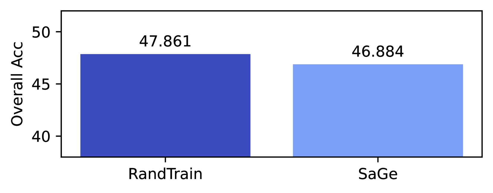</details> Figure 21: Comparison of SaGe and RandTrain, with $n$ -gram initial vocab, and FirstSpace pre-tokenization, $p$ =0.688 <details> <summary>x22.png Details</summary>  ### Visual Description ## Bar Chart: Overall Accuracy Comparison ### Overview The image displays a simple vertical bar chart comparing the "Overall Acc" (Overall Accuracy) of two distinct methods or models, labeled "RandTrain" and "SaGe". The chart presents a direct performance comparison, with numerical values annotated above each bar. ### Components/Axes * **Chart Type:** Vertical Bar Chart. * **Y-Axis:** * **Label:** "Overall Acc" (presumably Overall Accuracy). * **Scale:** Linear scale ranging from 40 to 50, with major tick marks at 40, 45, and 50. * **X-Axis:** * **Categories:** Two categorical bars. * **Labels:** "RandTrain" (left bar) and "SaGe" (right bar). * **Data Series & Legend:** There is no separate legend. The categories are identified by their x-axis labels. The bars are differentiated by color: * **RandTrain:** Dark blue bar. * **SaGe:** Light blue bar. * **Data Labels:** The exact numerical value of each bar's height is displayed directly above it. ### Detailed Analysis * **RandTrain (Dark Blue Bar):** * **Position:** Left side of the chart. * **Value:** 47.861 * **Visual Trend:** The bar extends from the baseline (below 40) to a height corresponding to approximately 47.9 on the y-axis. * **SaGe (Light Blue Bar):** * **Position:** Right side of the chart. * **Value:** 46.884 * **Visual Trend:** The bar is slightly shorter than the RandTrain bar, extending to a height corresponding to approximately 46.9 on the y-axis. * **Comparison:** The RandTrain method shows a higher overall accuracy than the SaGe method. The numerical difference is 47.861 - 46.884 = 0.977. ### Key Observations 1. **Close Performance:** The two methods have very similar performance levels, with less than a 1-point difference in overall accuracy. 2. **Visual Emphasis:** The y-axis is truncated, starting at 40 instead of 0. This visual choice amplifies the perceived difference between the two bars, making the ~1-point gap appear more significant than it would on a zero-based scale. 3. **Precision:** The accuracy values are reported to three decimal places, suggesting the measurements are precise and likely the result of a computational evaluation. ### Interpretation This chart provides a clear, at-a-glance comparison of two competing approaches ("RandTrain" and "SaGe") on a single metric: Overall Accuracy. The data suggests that **RandTrain has a slight performance advantage over SaGe** for the task being measured. The choice to truncate the y-axis is a common technique in technical presentations to highlight small but potentially meaningful differences. A reader should note that while RandTrain is superior in this specific comparison, the absolute difference is under 1%, which may or may not be practically significant depending on the application context (e.g., a 0.977% improvement in a medical diagnosis model is more impactful than in a recommendation system). The absence of error bars or confidence intervals means we cannot assess the statistical significance of this difference from the chart alone. The chart's primary function is to present the final, computed accuracy values for direct comparison. </details> Figure 22: Comparison of RandTrain and SaGe, with $n$ -gram initial vocab, and FirstSpaceDigit pre-tokenization, $p$ =0.15 We saw in Table 1 that both PathPieceL-BPE and SaGe-BPE are effective tokenizers. In attempting to isolate the benefit from the vocabulary construction step, we see that PathPieceL-BPE outperforms our simple baseline. However, SaGe was unable to outperform the baseline, perhaps implying that RandTrain may actually be a simple but fairly effective vocabulary construction method. ## Appendix G Detailed Experimental Results This section gives the detailed accuracy results for the 10 downstream evaluation tasks on each model that was trained. The tables are divided by the vocabulary size used, with Table 4 and Table 5 for 32,768; Table 6 and Table 7 for 40,960; and Table 8 and Table 9 for 49,152. The highest value or values (in the case of ties) are shown in bold. Table 10 show the same results as Table 1, but are sorted from best to worst by rank. The corpus token count (CTC), Rényi efficiencies, and average accuracies for the 54 runs in Figure 3 are given in Table 11. The detailed accuracy results for our 1.3B parameter models, which were all performed at a single vocabulary size of 40,960, are given in Table 12 and Table 13. Average accuracy results for larger models of 1.3B and 2.4B parameters are given in Table 14. See § Limitations for more discussion of this table. | Vocab Constr BPE | Init Voc FirstSpace | Pre-tok FirstSpace Greedy | Segment Merge 48.3 | Avg 48.8 51.9 | arc_easy 51.2 66.0 | copa 69.0 32.9 | mktg 32.9 23.7 | mathqa 23.9 65.6 | piqa 66.3 | | --- | --- | --- | --- | --- | --- | --- | --- | --- | --- | | FirstSpace | PathPieceL | 45.6 | 45.6 | 61.0 | 29.9 | 23.0 | 60.5 | | | | Unigram | | FirstSpace | Likelihood | 49.2 | 50.7 | 73.0 | 30.8 | 23.1 | 66.3 | | FirstSpace | Greedy | 47.9 | 50.3 | 68.0 | 31.2 | 23.1 | 65.2 | | | | FirstSpace | PathPieceL | 43.6 | 41.2 | 57.0 | 31.6 | 22.0 | 60.6 | | | | WordPiece | | FirstSpace | Greedy | 48.5 | 52.5 | 64.0 | 32.5 | 23.9 | 65.6 | | SaGe | BPE | FirstSpace | Greedy | 47.9 | 49.7 | 67.0 | 26.5 | 23.2 | 65.9 | | $n$ -gram | FirstSpDigit | Greedy | 48.4 | 50.3 | 71.0 | 29.5 | 22.0 | 65.1 | | | $n$ -gram | FirstSpace | Greedy | 47.5 | 48.8 | 64.0 | 29.5 | 23.0 | 66.6 | | | Unigram | FirstSpace | Greedy | 48.4 | 52.0 | 74.0 | 27.8 | 22.7 | 65.7 | | | PathPieceL | BPE | FirstSpace | PathPieceL | 49.3 | 50.8 | 68.0 | 34.2 | 23.0 | 66.4 | | $n$ -gram | FirstSpace | PathPieceL | 44.8 | 42.3 | 61.0 | 27.4 | 23.0 | 61.2 | | | $n$ -gram | FirstSpDigit | PathPieceL | 44.6 | 42.3 | 62.0 | 31.2 | 22.8 | 61.2 | | | Unigram | FirstSpace | PathPieceL | 46.9 | 50.4 | 64.0 | 24.8 | 23.5 | 66.2 | | | PathPieceR | $n$ -gram | FirstSpDigit | PathPieceR | 45.3 | 46.9 | 67.0 | 26.9 | 22.4 | 59.9 | | $n$ -gram | None | PathPieceR | 43.5 | 42.5 | 65.0 | 26.1 | 22.8 | 61.7 | | | $n$ -gram | SpaceDigit | PathPieceR | 47.5 | 48.6 | 68.0 | 32.9 | 23.3 | 65.0 | | | Random | | | | 32.0 | 25.0 | 50.0 | 25.0 | 20.0 | 50.00 | Table 4: 350M parameter model, 32,768 token vocabulary, accuracy (%) on average and initial 5 tasks | Vocab Constr BPE | Init Voc FirstSpace | Pre-tok FirstSpace Greedy | Segment Merge 27.5 | qa4mre 29.6 30.7 | race 29.2 88.0 | sciq 87.3 30.9 | sociology 30.9 66.3 | wsc273 67.8 | | --- | --- | --- | --- | --- | --- | --- | --- | --- | | FirstSpace | PathPieceL | 28.2 | 29.0 | 83.8 | 28.4 | 66.3 | | | | Unigram | | FirstSpace | Likelihood | 31.0 | 30.2 | 86.4 | 31.8 | 68.5 | | FirstSpace | Greedy | 28.9 | 30.6 | 86.9 | 31.8 | 62.6 | | | | FirstSpace | PathPieceL | 29.9 | 27.5 | 74.6 | 26.4 | 65.6 | | | | WordPiece | | FirstSpace | Greedy | 32.0 | 30.7 | 88.5 | 27.9 | 67.4 | | SaGe | BPE | FirstSpace | Greedy | 31.7 | 30.2 | 89.0 | 28.4 | 67.8 | | $n$ -gram | FirstSpDigit | Greedy | 31.0 | 30.3 | 86.6 | 32.3 | 66.0 | | | $n$ -gram | FirstSpace | Greedy | 30.0 | 31.0 | 87.8 | 25.9 | 68.5 | | | Unigram | FirstSpace | Greedy | 29.6 | 28.9 | 88.2 | 32.3 | 63.0 | | | PathPieceL | BPE | FirstSpace | PathPieceL | 28.5 | 31.1 | 88.8 | 35.3 | 67.0 | | $n$ -gram | FirstSpace | PathPieceL | 30.3 | 27.3 | 80.0 | 32.8 | 62.6 | | | $n$ -gram | FirstSpDigit | PathPieceL | 27.8 | 25.5 | 79.2 | 31.3 | 62.6 | | | Unigram | FirstSpace | PathPieceL | 29.6 | 30.6 | 87.6 | 24.4 | 68.1 | | | PathPieceR | $n$ -gram | FirstSpDigit | PathPieceR | 28.5 | 29.4 | 78.6 | 28.9 | 64.5 | | $n$ -gram | None | PathPieceR | 27.1 | 27.0 | 77.7 | 28.9 | 56.0 | | | $n$ -gram | SpaceDigit | PathPieceR | 25.0 | 29.4 | 85.7 | 32.3 | 64.8 | | | Random | | | | 25.0 | 25.0 | 25.0 | 25.0 | 50.0 | Table 5: 350M parameter model, 32,768 token vocabulary, accuracy (%) on remaining 5 tasks | Vocab Constr BPE | Init Voc FirstSpace | Pre-tok FirstSpace Greedy | Segment Merge 49.1 | Avg 50.0 52.3 | arc_easy 52.7 66.0 | copa 70.0 27.4 | mktg 31.6 22.9 | mathqa 24.3 66.9 | piqa 66.9 | | --- | --- | --- | --- | --- | --- | --- | --- | --- | --- | | FirstSpace | PathPieceL | 46.7 | 48.0 | 58.0 | 27.4 | 23.4 | 62.1 | | | | Unigram | | FirstSpace | Likelihood | 49.1 | 51.4 | 71.0 | 32.1 | 23.4 | 66.1 | | Unigram | | FirstSpace | Greedy | 48.5 | 49.9 | 64.0 | 30.3 | 23.3 | 65.7 | | Unigram | | FirstSpace | PathPieceL | 43.1 | 40.5 | 56.0 | 28.6 | 23.0 | 60.3 | | WordPiece | | FirstSpace | Greedy | 49.1 | 52.3 | 70.0 | 28.6 | 23.7 | 66.5 | | SaGe | BPE | FirstSpace | Greedy | 49.2 | 50.8 | 70.0 | 29.9 | 23.2 | 66.4 | | $n$ -gram | FirstSpDigit | Greedy | 46.9 | 48.4 | 67.0 | 30.3 | 22.6 | 64.0 | | | $n$ -gram | FirstSpace | Greedy | 48.5 | 49.8 | 68.0 | 32.9 | 22.8 | 65.4 | | | Unigram | FirstSpace | Greedy | 46.9 | 51.7 | 65.0 | 28.6 | 23.9 | 65.2 | | | PathPieceL | BPE | FirstSpace | PathPieceL | 49.4 | 52.1 | 71.0 | 29.9 | 23.9 | 66.9 | | $n$ -gram | FirstSpace | PathPieceL | 45.5 | 42.6 | 63.0 | 30.3 | 22.7 | 60.9 | | | $n$ -gram | FirstSpDigit | PathPieceL | 44.9 | 44.0 | 60.0 | 29.9 | 22.6 | 60.8 | | | Unigram | FirstSpace | PathPieceL | 48.5 | 51.7 | 71.0 | 31.2 | 24.2 | 66.2 | | | PathPieceR | $n$ -gram | FirstSpDigit | PathPieceR | 45.8 | 47.5 | 63.0 | 28.2 | 22.4 | 60.7 | | $n$ -gram | None | PathPieceR | 44.0 | 41.2 | 66.0 | 26.5 | 21.6 | 62.4 | | | $n$ -gram | SpaceDigit | PathPieceR | 45.4 | 46.3 | 64.0 | 32.1 | 22.7 | 60.0 | | | RandTrain | BPE | FirstSpace | Greedy | 48.6 | 50.5 | 70.0 | 29.5 | 23.4 | 65.8 | | $n$ -gram | FirstSpDigit | Greedy | 47.9 | 50.0 | 63.0 | 29.5 | 23.3 | 65.3 | | | $n$ -gram | FirstSpace | Greedy | 48.3 | 50.3 | 70.0 | 28.2 | 24.3 | 65.8 | | | $n$ -gram | None | Greedy | 42.2 | 41.3 | 55.0 | 27.4 | 21.7 | 63.2 | | | BPE | FirstSpace | PathPieceL | 46.5 | 45.8 | 65.0 | 30.8 | 23.3 | 62.8 | | | $n$ -gram | FirstSpDigit | PathPieceL | 38.8 | 31.2 | 48.0 | 27.8 | 22.6 | 54.7 | | | $n$ -gram | FirstSpace | PathPieceL | 40.0 | 30.7 | 55.0 | 26.5 | 20.8 | 55.4 | | | $n$ -gram | None | PathPieceL | 36.8 | 27.7 | 56.0 | 28.6 | 22.8 | 54.5 | | | random | | | | 32.0 | 25.0 | 50.0 | 25.0 | 20.0 | 50.0 | Table 6: 350M parameter model, 40,960 token vocabulary, accuracy (%) on average and initial 5 tasks | Vocab Constr BPE | Init Voc FirstSpace | Pre-tok FirstSpace Greedy | Segment Merge 31.7 | qa4mre 32.4 30.9 | race 30.1 88.3 | sciq 87.7 35.8 | sociology 35.3 68.9 | wsc273 69.2 | | --- | --- | --- | --- | --- | --- | --- | --- | --- | | FirstSpace | PathPieceL | 30.3 | 30.2 | 83.8 | 35.3 | 68.1 | | | | Unigram | | FirstSpace | Likelihood | 29.6 | 30.8 | 86.4 | 32.8 | 67.8 | | FirstSpace | Greedy | 32.4 | 29.6 | 86.7 | 32.8 | 70.3 | | | | FirstSpace | PathPieceL | 30.3 | 27.4 | 75.0 | 27.4 | 62.3 | | | | WordPiece | | FirstSpace | Greedy | 31.0 | 30.3 | 87.7 | 32.8 | 68.1 | | SaGe | BPE | FirstSpace | Greedy | 28.9 | 30.2 | 89.5 | 34.8 | 67.8 | | $n$ -gram | FirstSpDigit | Greedy | 30.6 | 28.1 | 85.8 | 32.3 | 59.7 | | | $n$ -gram | FirstSpace | Greedy | 29.2 | 30.0 | 88.4 | 33.3 | 65.2 | | | Unigram | FirstSpace | Greedy | 26.8 | 29.1 | 86.9 | 31.3 | 60.1 | | | PathPieceL | BPE | FirstSpace | PathPieceL | 31.0 | 29.6 | 87.3 | 34.3 | 67.8 | | $n$ -gram | FirstSpace | PathPieceL | 29.9 | 27.9 | 81.0 | 34.8 | 61.9 | | | $n$ -gram | FirstSpDigit | PathPieceL | 27.5 | 28.2 | 80.7 | 30.9 | 64.1 | | | Unigram | FirstSpace | PathPieceL | 31.3 | 29.7 | 86.3 | 29.9 | 63.7 | | | PathPieceR | $n$ -gram | FirstSpDigit | PathPieceR | 29.9 | 30.8 | 82.1 | 27.4 | 66.3 | | $n$ -gram | None | PathPieceR | 23.6 | 28.3 | 73.8 | 35.8 | 60.4 | | | $n$ -gram | SpaceDigit | PathPieceR | 27.5 | 28.7 | 78.2 | 31.3 | 63.0 | | | RandTrain | BPE | FirstSpace | Greedy | 32.0 | 29.6 | 86.9 | 30.9 | 67.4 | | $n$ -gram | FirstSpDigit | Greedy | 30.6 | 30.0 | 87.5 | 31.3 | 68.1 | | | $n$ -gram | FirstSpace | Greedy | 29.9 | 29.7 | 85.3 | 32.8 | 67.0 | | | $n$ -gram | None | Greedy | 28.2 | 27.8 | 75.9 | 26.4 | 55.0 | | | BPE | FirstSpace | PathPieceL | 32.8 | 28.5 | 80.3 | 30.9 | 64.5 | | | $n$ -gram | FirstSpDigit | PathPieceL | 31.3 | 24.2 | 62.1 | 30.4 | 55.3 | | | $n$ -gram | FirstSpace | PathPieceL | 28.9 | 23.6 | 66.8 | 33.8 | 59.0 | | | $n$ -gram | None | PathPieceL | 21.5 | 24.9 | 51.8 | 28.9 | 51.7 | | | random | | | | 25.0 | 25.0 | 25.0 | 25.0 | 50.0 | Table 7: 350M parameter model, 40,960 token vocabulary, accuracy (%) on remaining 5 tasks | Vocab Constr BPE | Init Voc FirstSpace | Pre-tok FirstSpace Greedy | Segment Merge 49.5 | Avg 48.1 53.9 | arc_easy 52.3 72.0 | copa 65.0 31.6 | mktg 31.6 24.2 | mathqa 23.7 68.4 | piqa 65.7 | | --- | --- | --- | --- | --- | --- | --- | --- | --- | --- | | FirstSpace | PathPieceL | 47.2 | 48.6 | 69.0 | 26.9 | 22.8 | 63.1 | | | | Unigram | | FirstSpace | Likelihood | 48.8 | 52.3 | 69.0 | 35.0 | 23.9 | 66.1 | | FirstSpace | Greedy | 48.6 | 51.6 | 68.0 | 32.1 | 24.4 | 65.7 | | | | FirstSpace | PathPieceL | 44.0 | 39.4 | 57.0 | 30.3 | 23.3 | 61.2 | | | | WordPiece | | FirstSpace | Greedy | 48.8 | 52.6 | 68.0 | 28.2 | 23.5 | 66.2 | | SaGe | BPE | FirstSpace | Greedy | 48.8 | 51.9 | 71.0 | 29.9 | 22.6 | 65.5 | | $n$ -gram | FirstSpDigit | Greedy | 47.2 | 46.6 | 67.0 | 31.2 | 22.7 | 63.4 | | | $n$ -gram | FirstSpace | Greedy | 48.0 | 49.7 | 66.0 | 31.6 | 21.6 | 65.7 | | | Unigram | FirstSpace | Greedy | 47.8 | 49.7 | 68.0 | 29.9 | 23.5 | 64.6 | | | PathPieceL | BPE | FirstSpace | PathPieceL | 49.4 | 51.9 | 69.0 | 29.9 | 24.5 | 66.6 | | $n$ -gram | FirstSpace | PathPieceL | 43.9 | 42.4 | 56.0 | 28.6 | 23.8 | 60.3 | | | $n$ -gram | FirstSpDigit | PathPieceL | 45.0 | 44.5 | 59.0 | 28.2 | 22.3 | 59.5 | | | Unigram | FirstSpace | PathPieceL | 48.4 | 51.4 | 67.0 | 29.5 | 24.7 | 65.2 | | | PathPieceR | $n$ -gram | FirstSpDigit | PathPieceR | 45.5 | 46.0 | 62.0 | 25.6 | 22.1 | 61.6 | | $n$ -gram | None | PathPieceR | 42.2 | 42.6 | 64.0 | 22.2 | 22.4 | 60.9 | | | $n$ -gram | SpaceDigit | PathPieceR | 47.3 | 48.7 | 68.0 | 34.2 | 21.9 | 65.1 | | | random | | | | 32.0 | 25.0 | 50.0 | 25.0 | 20.0 | 50.0 | Table 8: 350M parameter model, 49,152 token vocabulary, accuracy (%) on average and initial 5 tasks | Vocab Constr BPE | Init Voc FirstSpace | Pre-tok FirstSpace Greedy | Segment Merge 29.6 | qa4mre 28.9 31.2 | race 31.0 88.4 | sciq 87.3 29.4 | sociology 28.9 66.3 | wsc273 67.0 | | --- | --- | --- | --- | --- | --- | --- | --- | --- | | FirstSpace | PathPieceL | 31.0 | 30.7 | 85.4 | 31.8 | 63.0 | | | | Unigram | | FirstSpace | Likelihood | 27.5 | 30.3 | 89.1 | 28.9 | 65.9 | | FirstSpace | Greedy | 32.4 | 29.5 | 86.7 | 32.3 | 63.7 | | | | FirstSpace | PathPieceL | 33.1 | 26.0 | 74.5 | 27.9 | 67.0 | | | | WordPiece | | FirstSpace | Greedy | 29.2 | 31.1 | 88.0 | 34.3 | 66.7 | | SaGe | BPE | FirstSpace | Greedy | 29.6 | 31.2 | 87.5 | 32.3 | 65.9 | | $n$ -gram | FirstSpDigit | Greedy | 29.2 | 28.8 | 86.4 | 34.3 | 61.9 | | | $n$ -gram | FirstSpace | Greedy | 28.8 | 30.2 | 87.5 | 33.8 | 64.5 | | | Unigram | FirstSpace | Greedy | 28.9 | 31.4 | 87.0 | 29.9 | 65.6 | | | PathPieceL | BPE | FirstSpace | PathPieceL | 31.0 | 31.4 | 87.5 | 31.3 | 70.7 | | $n$ -gram | FirstSpace | PathPieceL | 27.5 | 26.7 | 80.8 | 32.3 | 60.8 | | | $n$ -gram | FirstSpDigit | PathPieceL | 28.9 | 30.0 | 80.6 | 35.8 | 61.2 | | | Unigram | FirstSpace | PathPieceL | 29.2 | 30.5 | 88.5 | 32.8 | 65.6 | | | PathPieceR | $n$ -gram | FirstSpDigit | PathPieceR | 29.6 | 29.5 | 82.8 | 30.9 | 64.5 | | $n$ -gram | None | PathPieceR | 25.7 | 27.5 | 72.5 | 27.4 | 57.1 | | | $n$ -gram | SpaceDigit | PathPieceR | 27.5 | 28.7 | 84.0 | 28.9 | 66.3 | | | Random | | | | 25.0 | 25.0 | 25.0 | 25.0 | 50.0 | Table 9: 350M parameter model, 49,152 token vocabulary, accuracy (%) on remaining 5 tasks | 1 | PathPieceL | BPE | FirstSpace | PathPieceL | 49.4 | 49.3 | 49.4 | 49.4 | | --- | --- | --- | --- | --- | --- | --- | --- | --- | | 2 | Unigram | | FirstSpace | Likelihood | 49.0 | 49.2 | 49.1 | 48.8 | | 3 | BPE | | FirstSpace | Merge | 49.0 | 48.8 | 50.0 | 48.1 | | 4 | BPE | | FirstSpace | Greedy | 49.0 | 48.3 | 49.1 | 49.5 | | 5 | WordPiece | | FirstSpace | Greedy | 48.8 | 48.5 | 49.1 | 48.8 | | 6 | SaGe | BPE | FirstSpace | Greedy | 48.6 | 47.9 | 49.2 | 48.8 | | 7 | Unigram | | FirstSpace | Greedy | 48.3 | 47.9 | 48.5 | 48.6 | | 8 | SaGe | $n$ -gram | FirstSpace | Greedy | 48.0 | 47.5 | 48.5 | 48.0 | | 9 | PathPieceL | Unigram | FirstSpace | PathPieceL | 48.0 | 46.9 | 48.5 | 48.4 | | 10 | SaGe | Unigram | FirstSpace | Greedy | 47.7 | 48.4 | 46.9 | 47.8 | | 11 | SaGe | $n$ -gram | FirstSpDigit | Greedy | 47.5 | 48.4 | 46.9 | 47.2 | | 12 | PathPieceR | $n$ -gram | SpaceDigit | PathPieceR | 46.7 | 47.5 | 45.4 | 47.3 | | 13 | BPE | | FirstSpace | PathPieceL | 46.5 | 45.6 | 46.7 | 47.2 | | 14 | PathPieceR | $n$ -gram | FirstSpDigit | PathPieceR | 45.5 | 45.3 | 45.8 | 45.5 | | 15 | PathPieceL | $n$ -gram | FirstSpDigit | PathPieceL | 44.8 | 44.6 | 44.9 | 45.0 | | 16 | PathPieceL | $n$ -gram | FirstSpace | PathPieceL | 44.7 | 44.8 | 45.5 | 43.9 | | 17 | Unigram | | FirstSpace | PathPieceL | 43.6 | 43.6 | 43.1 | 44.0 | | 18 | PathPieceR | $n$ -gram | None | PathPieceR | 43.2 | 43.5 | 44.0 | 42.2 | | Random | | | | 32.0 | 32.0 | 32.0 | 32.0 | | Table 10: Summary of 350M parameter model downstream accuracy (%), sorted by rank | 1 1 1 | 32,768 40,960 49,152 | 49.3 49.4 49.4 | 1.48 1.46 1.44 | 0.604 0.589 0.578 | 0.516 0.503 0.492 | 0.469 0.457 0.448 | 0.441 0.429 0.420 | 0.422 0.411 0.402 | | --- | --- | --- | --- | --- | --- | --- | --- | --- | | 2 | 32,768 | 49.2 | 1.79 | 0.461 | 0.371 | 0.324 | 0.295 | 0.277 | | 2 | 40,960 | 49.1 | 1.77 | 0.451 | 0.362 | 0.316 | 0.289 | 0.271 | | 2 | 49,152 | 48.8 | 1.76 | 0.444 | 0.356 | 0.311 | 0.284 | 0.266 | | 3 | 32,768 | 48.8 | 1.52 | 0.594 | 0.505 | 0.459 | 0.431 | 0.414 | | 3 | 40,960 | 50.0 | 1.49 | 0.579 | 0.491 | 0.446 | 0.420 | 0.403 | | 3 | 49,152 | 48.1 | 1.47 | 0.567 | 0.481 | 0.437 | 0.411 | 0.394 | | 4 | 32,768 | 48.3 | 1.50 | 0.605 | 0.517 | 0.471 | 0.442 | 0.423 | | 4 | 40,960 | 49.1 | 1.48 | 0.590 | 0.504 | 0.458 | 0.430 | 0.412 | | 4 | 49,152 | 49.5 | 1.46 | 0.579 | 0.494 | 0.449 | 0.421 | 0.403 | | 5 | 32,768 | 48.5 | 1.54 | 0.598 | 0.507 | 0.461 | 0.433 | 0.415 | | 5 | 40,960 | 49.1 | 1.51 | 0.583 | 0.494 | 0.448 | 0.421 | 0.404 | | 5 | 49,152 | 48.8 | 1.49 | 0.571 | 0.483 | 0.439 | 0.412 | 0.396 | | 6 | 32,768 | 47.9 | 1.78 | 0.545 | 0.466 | 0.422 | 0.396 | 0.378 | | 6 | 40,960 | 49.2 | 1.76 | 0.533 | 0.455 | 0.413 | 0.387 | 0.369 | | 6 | 49,152 | 48.7 | 1.75 | 0.523 | 0.447 | 0.405 | 0.379 | 0.362 | | 7 | 32,768 | 47.9 | 1.81 | 0.510 | 0.431 | 0.387 | 0.359 | 0.340 | | 7 | 40,960 | 48.5 | 1.79 | 0.500 | 0.423 | 0.381 | 0.354 | 0.335 | | 7 | 49,152 | 48.6 | 1.77 | 0.493 | 0.416 | 0.375 | 0.348 | 0.330 | | 8 | 32,768 | 47.5 | 1.63 | 0.629 | 0.536 | 0.482 | 0.447 | 0.424 | | 8 | 40,960 | 48.5 | 1.62 | 0.615 | 0.524 | 0.470 | 0.437 | 0.415 | | 8 | 49,152 | 48.0 | 1.62 | 0.605 | 0.515 | 0.462 | 0.429 | 0.407 | | 9 | 32,768 | 46.9 | 1.74 | 0.508 | 0.419 | 0.372 | 0.343 | 0.323 | | 9 | 40,960 | 48.5 | 1.72 | 0.491 | 0.403 | 0.356 | 0.328 | 0.309 | | 9 | 49,152 | 48.4 | 1.72 | 0.477 | 0.389 | 0.343 | 0.315 | 0.296 | | 10 | 32,768 | 48.4 | 2.02 | 0.485 | 0.409 | 0.366 | 0.339 | 0.320 | | 10 | 40,960 | 46.9 | 2.01 | 0.474 | 0.401 | 0.358 | 0.331 | 0.313 | | 10 | 49,152 | 47.8 | 2.01 | 0.466 | 0.393 | 0.352 | 0.325 | 0.307 | | 11 | 32,768 | 48.4 | 1.77 | 0.587 | 0.512 | 0.470 | 0.443 | 0.425 | | 11 | 40,960 | 46.9 | 1.76 | 0.575 | 0.501 | 0.460 | 0.433 | 0.415 | | 11 | 49,152 | 47.2 | 1.76 | 0.565 | 0.492 | 0.452 | 0.426 | 0.408 | | 12 | 32,768 | 47.5 | 2.33 | 0.236 | 0.164 | 0.138 | 0.124 | 0.116 | | 12 | 40,960 | 45.4 | 2.30 | 0.228 | 0.159 | 0.133 | 0.120 | 0.112 | | 12 | 49,152 | 47.3 | 2.29 | 0.223 | 0.155 | 0.130 | 0.117 | 0.109 | | 13 | 32,768 | 45.6 | 1.50 | 0.606 | 0.518 | 0.470 | 0.442 | 0.423 | | 13 | 40,960 | 46.7 | 1.47 | 0.591 | 0.504 | 0.458 | 0.430 | 0.412 | | 13 | 49,152 | 47.2 | 1.45 | 0.579 | 0.494 | 0.449 | 0.421 | 0.403 | | 14 | 32,768 | 45.3 | 1.46 | 0.616 | 0.532 | 0.490 | 0.465 | 0.448 | | 14 | 40,960 | 45.8 | 1.43 | 0.602 | 0.519 | 0.478 | 0.453 | 0.437 | | 14 | 49,152 | 45.5 | 1.42 | 0.591 | 0.508 | 0.468 | 0.444 | 0.428 | | 15 | 32,768 | 44.6 | 1.47 | 0.620 | 0.533 | 0.490 | 0.464 | 0.447 | | 15 | 40,960 | 44.9 | 1.44 | 0.605 | 0.520 | 0.478 | 0.453 | 0.436 | | 15 | 49,152 | 45.0 | 1.42 | 0.594 | 0.509 | 0.468 | 0.443 | 0.427 | | 16 | 32,768 | 44.8 | 1.36 | 0.677 | 0.571 | 0.514 | 0.480 | 0.457 | | 16 | 40,960 | 45.5 | 1.33 | 0.662 | 0.556 | 0.500 | 0.466 | 0.444 | | 16 | 49,152 | 43.9 | 1.31 | 0.650 | 0.544 | 0.489 | 0.456 | 0.435 | | 17 | 32,768 | 43.6 | 1.77 | 0.471 | 0.380 | 0.333 | 0.304 | 0.285 | | 17 | 40,960 | 43.1 | 1.75 | 0.462 | 0.372 | 0.326 | 0.298 | 0.280 | | 17 | 49,152 | 44.0 | 1.74 | 0.455 | 0.366 | 0.320 | 0.293 | 0.275 | | 18 | 32,768 | 43.5 | 1.29 | 0.747 | 0.617 | 0.549 | 0.511 | 0.486 | | 18 | 40,960 | 44.0 | 1.26 | 0.736 | 0.603 | 0.535 | 0.497 | 0.474 | | 18 | 49,152 | 42.2 | 1.25 | 0.728 | 0.591 | 0.524 | 0.487 | 0.464 | Table 11: Average Accuracy (%) vs. Corpus Token Count (CTC, in billions) by vocabulary size, for Figure 3. Also includes the corresponding Rényi efficiency (Zouhar et al., 2023a) for various orders $α$ . | Vocab Constr | Init Voc | Pre-tok | Segment | Avg | arc_easy | copa | mktg | mathqa | piqa | | --- | --- | --- | --- | --- | --- | --- | --- | --- | --- | | BPE | | FirstSpace | Merge | 53.1 | 62.0 | 77.0 | 32.1 | 25.0 | 71.1 | | Unigram | | FirstSpace | Likelihood | 52.4 | 60.6 | 71.0 | 30.3 | 25.2 | 71.0 | | SaGe | BPE | FirstSpace | Greedy | 52.2 | 62.0 | 72.0 | 27.4 | 24.5 | 71.6 | | $n$ -gram | FirstSpDigit | Greedy | 50.7 | 60.3 | 71.0 | 28.6 | 22.8 | 69.4 | | | PathPieceL | BPE | FirstSpace | PathPieceL | 49.2 | 57.4 | 66.0 | 27.8 | 24.3 | 65.9 | | $n$ -gram | FirstSpDigit | PathPieceL | 47.6 | 49.7 | 67.0 | 24.8 | 23.4 | 63.2 | | | $n$ -gram | SpaceDigit | PathPieceL | 46.3 | 51.1 | 59.0 | 28.6 | 23.3 | 63.8 | | | Random | | | | 32.0 | 25.0 | 50.0 | 25.0 | 20.0 | 50.0 | Table 12: 1.3B parameter model, 40,960 token vocabulary, accuracy (%) on average and initial 5 tasks | Vocab Constr | Init Voc | Pre-tok | Segment | qa4mre | race | sciq | sociology | wsc273 | | --- | --- | --- | --- | --- | --- | --- | --- | --- | | BPE | | FirstSpace | Merge | 32.4 | 34.9 | 93.0 | 26.4 | 76.9 | | Unigram | | FirstSpace | Likelihood | 37.7 | 33.0 | 91.8 | 28.9 | 74.4 | | SaGe | BPE | FirstSpace | Greedy | 34.9 | 34.8 | 92.5 | 25.9 | 76.2 | | $n$ -gram | FirstSpDigit | Greedy | 29.9 | 32.9 | 91.5 | 29.4 | 71.1 | | | PathPieceL | BPE | FirstSpace | PathPieceL | 31.0 | 33.3 | 89.4 | 26.4 | 70.7 | | $n$ -gram | FirstSpDigit | PathPieceL | 31.0 | 31.6 | 86.1 | 29.4 | 70.0 | | | $n$ -gram | SpaceDigit | PathPieceL | 28.9 | 31.3 | 87.1 | 22.4 | 67.0 | | | Random | | | | 25.0 | 25.0 | 25.0 | 25.0 | 50.0 | Table 13: 1.3B parameter model, 40,960 token vocabulary, accuracy (%) on remaining 5 tasks | Voc Con | Init V | Pre-tok | Seg | 350M avg | 350M rnk | 1.3B avg | 1.3B rnk | 2.4B avg | 2.4B rnk | | --- | --- | --- | --- | --- | --- | --- | --- | --- | --- | | BPE | | FirSp | Merge | 50.0 | 1 | 53.1 | 1 | 54.2 | 3 | | PathPL | BPE | FirSp | PathPL | 49.4 | 3 | 49.2 | 5 | 52.7 | 4 | | PathPL | $n$ -gram | FirSpD | PathPL | 44.9 | 6 | 47.6 | 6 | | | | SaGe | BPE | FirSp | Greedy | 49.2 | 2 | 52.2 | 3 | 55.0 | 1 | | SaGe | $n$ -gram | FirSpD | Greedy | 46.9 | 5 | 50.7 | 4 | | | | Unigram | | FirSp | Likeli | 49.1 | 4 | 52.4 | 2 | 54.7 | 2 | Table 14: Downstream accuracy (%) of 10 tasks with vocab size 40,960, for various model sizes