2403.06309

# Use of Nash equilibrium in finding game theoretic robust security bound on quantum bit error rate **Authors**: Arindam Dutta, Anirban Pathak > Department of Physics and Materials Science & Engineering, Jaypee Institute of Information Technology, A 10, Sector 62, Noida, UP-201309, India ## Abstract Nash equilibrium is employed to find a game theoretic robust security bound on quantum bit error rate (QBER) for DL04 protocol which is a scheme for quantum secure direct communication that has been experimentally realized recently. The receiver, sender and eavesdropper (Eve) are considered to be quantum players (players having the capability to perform quantum operations). Specifically, Eve is considered to have the capability of performing quantum attacks (e.g., Wójcik’s original attack, Wójcik’s symmetrized attack and Pavičić attack) and classical intercept and resend attack. Game theoretic analysis of the security of DL04 protocol in the above scenario is performed by considering several game scenarios. The analysis revealed the absence of a Pareto optimal Nash equilibrium point within these game scenarios. Consequently, mixed strategy Nash equilibrium points are identified and employed to establish both upper and lower bounds for QBER. Further, the vulnerability of the DL04 protocol to Pavičić attack in the message mode is established. In addition, it is observed that the quantum attacks performed by Eve are more powerful than the classical attack, as the QBER value and the probability of detecting Eve’s presence are found to be lower in quantum attacks compared to classical ones. ## I Introduction Game theory examines and models how individuals behave in situations involving strategic (rational) thinking and interactive decision-making. It is crucial for decision-making processes and assessing opportunities, both in business and everyday scenarios. Instances requiring strategic thinking are prevalent in fields such as economics [1], political science [2], biology [3, 4] and military applications [5, 6]. Participants in these scenarios have their own sets of potential actions, referred to as strategies, and express preferences for these actions through a payoff matrix. Game theory is concerned with representing these activities and identifying optimal strategies. Among the various concepts in game theory, the Nash equilibrium is particularly significant. It characterizes the optimal decisions considering the actions of other players. In a Nash equilibrium, no player stands to benefit by altering their strategy alone [7, 8]. Quantum mechanics stands out as one of the most influential theories throughout history. Despite the controversies it has sparked since its inception, its predictions have been consistently and precisely confirmed through experiments [9]. Quantum game theory enables the examination of interactive decision-making scenarios involving players utilizing quantum technology. This technology serves a dual purpose: functioning as a quantum communication protocol and providing a more efficient method for randomizing players’ strategies compared to classical games [10]. Quantum game theory emanated in 1999 through the contributions of David Meyer [11], and Jens Eisert, Martin Wilkens and Maciej Lewenstein [12]. Their research explored games that incorporated quantum information, showcasing scenarios where quantum players demonstrated advantages over their classical counterparts. Subsequently, numerous examples of quantum games, largely built upon the foundations established by Meyer, and Eisert, Wilkens and Lewenstein, have been extensively examined. Further details and references can be found in surveys such as [13]. In the realm of experiments, researchers have successfully implemented the quantum version of the Prisoners’ Dilemma game using an NMR quantum computer [14]. Additionally, Vaidman [15] demonstrated a simple game wherein players consistently emerge victorious if they share a GHZ state beforehand, contrasting with classical players where winning is always subject to probability. Quantum strategies have been employed to introduce fairness elements into remote gambling scenarios [16] and in formulating algorithms for quantum auctions, which come with numerous security advantages [17]. Flitney and Abbott [18] have explored quantum adaptations of Parrondo’s games. Such analyses not only aid in designing secure networks leading to the identification of novel quantum algorithms but also add an entirely distinct dimension to characterizing a game or a protocol [19, 20, 21]. Furthermore, eavesdropping [22, 23] and optimal cloning [24] can be conceptualized as games played between participants. Thus, an interconnection between game theory and quantum mechanics is already explored. There are primarily two approaches that illustrate this interconnection. In the first approach, quantum resources are used to play a traditional game that can also be played without any quantum resources, but the use of quantum resources provide some advantages, whereas in the second approach, a quantum mechanical scenario is described using the concepts of the game theory. In what follows, the first (second) approach mentioned above is referred to as the quantized game (gaming the quantum). Here, it will be apt to note that a quantized game can be defined as a unitary function mapping the Cartesian product of sets of quantum superpositions of players’ pure strategies to the entire Hilbert space encompassing the domain of the game. This retains the characteristics of the original game under specific conditions. On the other hand, the concept of gaming the quantum [25] refers to the application(s) of the principles of game theory to quantum mechanics to derive game-theoretic solutions. In this study, we do “gaming the quantum” by applying non-cooperative game theory to a quantum communication protocol to demonstrate how Nash equilibrium can serve as a viable solution concept. By drawing motivation from the aforementioned facts, we can leverage Nash equilibrium points in a game to establish secure bounds for various quantum information parameters. This involves transforming any quantum scheme into a scenario resembling a game and examining Nash equilibrium points. Nash equilibrium points serve as stable conditions or provide optimistic and rational probabilities for stakeholders to make decisions within a mixed strategic game framework. Utilizing these probabilities derived from Nash equilibrium points facilitates the establishment of a stable gaming environment for all parties involved. This enables the assessment of various cryptography parameters, including determining the threshold value of quantum bit error rate (QBER). In a practical context where decisions are autonomously made by each party, attaining a stable point is less probable and could result in increased instability. Consequently, identifying the minimum QBER value from the stable gaming scenario sets a secure threshold boundary for the practical deployment of the protocols for secure quantum communication. In our paper, we specifically delve into the investigation of the secure threshold bound for the QBER in the context of the DL04 protocol [26]. It is crucial to emphasize the context of direct secure quantum communication protocols as the DL04 scheme belongs to this category. The direct secure quantum communication protocols can be broadly categorized into two classes [27]. First, there are the deterministic secure quantum communication (DSQC) protocols [28, 29, 30, 31], where the receiver can decode the secret message sent by the sender only after transmission of at least one bit of additional classical information for each qubit. Second, there are the quantum secure direct communication (QSDC) protocols [32, 33, 34, 35, 26, 36, 37, 38, 39], which do not necessitate any exchange of classical information. Beige et al. introduced a QSDC scheme [32]. In this proposal, the message is accessible only following the transmission of additional classical information for each qubit. Boström and Felbinger presented a ping-pong QSDC scheme [34], which is secure for key distribution and quasi-secure for direct secret communication when employing a perfect quantum channel. In 2004, Deng and Long [26] put forth a QSDC protocol (DL04 protocol) that does not rely on entangled states. An unexpected finding is the ability to ensure secure information transmission through the two-photon component, aligning with the outcomes observed in two-way quantum key distribution (QKD) [40, 41, 42]. This aligns with the specific scenario presented in the DL04 QSDC protocol [26]. Our primary focus in this study is on estimating the secure threshold bound of QBER within the DL04 protocol. This choice is motivated by its widespread acceptance for experimental realization and its feasibility for secure implementation [43, 44, 45, 46, 47, 48, 49]. The remainder of the paper is structured as follows. In Section II, we begin with a lucid introduction to game theory restricted to the context of the present paper as game theory serves as the basis for our analysis. In this section, we also define the DL04 protocol as a scenario resembling a game. Moving on to Section III, we present the mathematical formulation of our game and employ a graphical method to examine the Nash equilibrium. Additionally, we scrutinize the Nash equilibrium points to determine the secure threshold bound of QBER for the DL04 protocol. Finally, Section IV provides a summary and discussion of our findings, serving as the conclusion of the paper. In addition, detailed mathematical proofs and details of the analysis presented in various sections are presented in Appendices A-E. ## II Preliminaries of Game Theory Before we delve into the technical details of our work, it will be apt to briefly introduce the basics of game theory. Game theory comprises a set of mathematical models designed to examine scenarios involving both competition and collaboration, where an individual’s (player’s) ability to make choices effectively relies on the choices made by others. Each player has a set of possible strategies or actions they can take. This strategy is a plan or decision that specifies how a player will act in different situations within the game. The primary objective is to identify optimal strategies for individuals facing such situations and to identify equilibrium states. The outcomes of a game are often represented in terms of payoffs, which measure the utility or satisfaction that each player receives based on the chosen strategies of all players. Payoffs can be represented in various forms, such as numerical values, rankings or other measures. Game theory can be represented in different forms; the normal form (strategic form) is a matrix that shows the payoffs for each combination of strategies chosen by the players. The extensive form (dynamic game) uses a tree-like diagram to represent sequential and simultaneous decision-making. There are mainly two types of games, zero-sum games and non-zero-sum games. In a zero-sum game, the total payoff is constant, and gains for one player result in losses for the other player(s). In non-zero-sum games, the total payoff can vary, and the interests of the players may not be directly opposed. An important fundamental concept in game theory is Nash equilibrium which corresponds to a set of strategies in which no player has an incentive to unilaterally change their strategy, given the strategies chosen by the other players. It represents a stable solution where no player can improve their payoff by changing their strategy. A game’s strategy set is considered Pareto efficient (or Pareto optimal) when there does not exist another strategy set that can improve the outcome for one player without negatively affecting any other player. Further, a dominant strategy is a strategy that is always the best choice for a player, regardless of the strategies chosen by other players. A dominant strategy is a strong concept in rational decision-making. When a player follows a pure strategy, they choose a single action or decision without any randomness or uncertainty. In some games, players may adopt mixed strategies, where they choose their actions with certain probabilities. Mixed strategies can lead to a Nash equilibrium when no pure strategy is optimal [12, 50, 51, 52, 53]. Quantum game In a traditional game that allows for the use of mixed strategies, players construct their strategies by using real coefficients to form convex linear combinations of their pure strategies [54]. In contrast, in a quantum game [12, 55], players employ unitary transformations and quantum states that belong to substantially larger strategy spaces. This has led to discussions proposing that quantum games could be considered extensions of classical games, potentially offering stakeholders a quantum advantage in the game [56]. As mentioned earlier, it is important to emphasize that any quantum protocol (quantum cryptographic scenarios) can be analogized to a game-like scenario. In this context, participants’ strategies hinge on the utilization of unitary operations and the selection of measurement bases, with the final payoff determined by the results of the measurements. Quantum advantage arises from the optimal sequential utilization of quantum operations on quantum states by the players. Typically, in traditional quantum game theory paper classical players are limited to using coherent permutations of standard basis states, or similarly restricted types of unitary operations. In contrast, quantum players have access to a wider range of available unitary operations, which may include the full spectrum of such operations with fewer limitations. Before we proceed further, it will be appropriate to formally discuss pure quantum strategy, mixed quantum strategy and positive operator valued measure (POVM) quantum strategy [55] in the context of the present work. A pure quantum strategy involves deterministic actions, represented by unitary operations on the player’s quantum state. This strategy starts with a quantum state $|\Psi\rangle$ in a Hilbert space $\mathcal{H}$ . Each player $i$ selects a unitary operation $U_{i}$ to apply to their portion of the quantum state. After all players have applied their respective unitary operations, the resulting quantum state is $|\Psi_{f}\rangle=\left(U_{1}\otimes U_{2}\otimes\cdots\otimes U_{i}\otimes \cdots\otimes U_{n}\right)$ , where $n$ denotes the total number of players in a game. The final state $|\Psi_{f}\rangle$ is then measured to determine the outcome of the game. On the other hand, a mixed quantum strategy involves probabilistic combinations of various pure quantum strategies. Starting with the same initial state as in the pure strategy, each player $i$ has a set of pure strategies $\left\{U_{i}^{1},U_{i}^{2},\cdots,U_{i}^{k}\right\}$ and an associated probability distribution $\left\{p_{i}^{1},p_{i}^{2},\cdots,p_{i}^{k}\right\}$ , where $\stackrel{{\scriptstyle[}}{{j}}=1]{k}{\sum}p_{i}^{j}=1$ . Each player $i$ randomly selects a unitary operation $U_{i}$ with probability $p_{i}^{j}$ . Consequently, the ensemble of possible final states is a mixture of pure states, represented by the mixed state $\rho_{f}=\underset{j}{\sum}p_{i}^{j}\left(U_{i}^{j}\otimes\cdots\otimes U_{n}^ {j}\right)|\Psi\rangle\langle\Psi|\left(U_{i}^{j}\otimes\cdots\otimes U_{n}^{j }\right)^{\dagger}$ . This mixed state $\rho_{f}$ is then measured to determine the game’s outcome. A POVM quantum strategy employs general quantum measurements, defined by a set of POVM elements. Starting with the initial state $|\Psi\rangle$ , each player $i$ uses a POVM, which consists of positive semi-definite operators $\left\{\mathcal{E}_{i}^{1},\mathcal{E}_{i}^{2},\cdots,\mathcal{E}_{i}^{k}\right\}$ that satisfy $\underset{j}{\sum}\mathcal{E}_{i}^{j}=\mathds{1}$ . The POVM elements are applied to the quantum state, with outcome $j$ occurring with probability $p_{i}^{j}=\langle\Psi|E_{i}^{j}|\Psi\rangle$ . Depending on the measurement outcome, players may apply conditional unitary operations or other quantum operations. The final state, which depends on the measurement outcomes and subsequent operations, is given by $\rho_{f}=\underset{j}{\sum}\left(U_{i}^{j}\otimes\cdots\otimes U_{i}^{j}\right )\mathcal{E}_{i}^{j}|\Psi\rangle\langle\Psi|\mathcal{E}_{i}^{j}\left(U_{i}^{j} \otimes\cdots\otimes U_{i}^{j}\right)^{\dagger}$ . This final state $\rho_{f}$ is measured to determine the game’s outcome. Each type of strategy improves in generality and flexibility, with POVM quantum strategies covering the widest range of possible actions within quantum game theory. In our work, we have implemented a mixed quantum strategy in which Alice, Bob and Eve perform their quantum operations with specific probabilistic combinations to get Nash equilibrium points. The final mixed state determines the payoff elements for each respective player. Our considered game, which is a non-cooperative quantum game involving multiple players, lacks a pure strategy Nash equilibrium. This is due to the nature of the multiplayer model and the way payoffs are calculated, similar to the approach in [25]. Furthermore, the concept of a Nash equilibrium solution is fundamental in game theory as it can be used to predict the behavior of non-cooperating players. The proof of Nash’s theorem for the existence of an equilibrium in mixed strategies in traditional games is relatively simple and relies entirely on Kakutani’s fixed-point theorem [57]. In the realm of quantum games, Meyer demonstrated the existence of Nash equilibrium in mixed strategies, which are represented as mixed quantum states, by employing Glicksberg’s [58] extension of Kakutani’s fixed-point theorem to topological vector spaces. In 2019, Khan et al. found that the Kakutani fixed-point theorem does not directly apply to quantum games involving pure quantum strategies [59]. However, by using Nash’s embedding theorem, which embeds compact Riemannian manifolds into Euclidean space [60], and under certain conditions, the Kakutani fixed-point theorem can be indirectly applied to ensure Nash equilibrium in pure quantum strategies. They did a formal mathematical discussion of non-cooperative game theory and fixed points (see Ref. [59] for details). Our contribution In our game, several key points should be noted as it is a mixed quantum strategic game. When players can choose their quantum strategies based on a probability distribution, thereby using mixed quantum strategies, Meyer demonstrated through Glicksberg’s fixed-point theorem [58] that a Nash equilibrium will always be present. Meyer’s research also offers insights into the equilibrium behavior of quantum computational mechanisms. His approach to identifying quantum advantage as a Nash equilibrium in quantum games remains largely unexplored [61]. Additionally, in the realm of quantum communication protocols, where quantum processes are typically noisy and represented as density matrices or mixed quantum states, the Meyer–Glicksberg theorem ensures the existence of a Nash equilibrium [11]. Generally, in quantum communication protocols, less restricted quantum players can utilize their mixed strategies to calculate their individual best response functions based on their payoffs. The solutions of best response functions give the Nash equilibrium points. While not all of these points may be Pareto optimal Nash equilibrium points, they serve as a basis for determining the probabilities of mixed strategies employed by the players. This, in turn, allows for an investigation into the existence of Pareto optimal Nash equilibrium points. The outcome of this analysis helps to determine the secure bounds for various quantum information parameters (e.g., secret key rate, QBER) with appropriate use of the fundamental concepts of quantum information theory [62, 63, 64, 65]. In our letter, we take the DL04 protocol [26] and analyze it as a game, considering different types of attack (collective attacks and IR attack) to get the secure threshold limit for QBER. In quantum cryptography, QSDC employs quantum states as carriers of information for secure communication. Unlike traditional methods, QSDC does not require a prior generation of secret key [32, 33, 34, 35, 26, 36, 37]. It is a concept centered around achieving secure and reliable communication through the principles of quantum physics. Extensive experimental studies on QSDC have demonstrated its feasibility and promising application prospects [43, 66, 67, 45, 68, 47, 69, 70, 48]. After more than two decades of persistent effort, QSDC is gradually maturing and showing significant potential for advancing next-generation secure communication [71], including potential applications in military contexts [72]. Among different protocols for QSDC that have been proposed till date, the DL04 protocol needs special mention as the recent experimental activities [43, 44, 45, 46, 47, 48, 49] are centered around it. Keeping this in mind, in what follows we focus our work on the DL04 protocol specifically though the strategy developed here is general in nature. Let us commence with a concise overview of the DL04 protocol [26], slightly modified to align with a gaming scenario. Within this framework, Bob, at random, generates quantum states (photons) $|0\rangle$ and $|1\rangle$ in the computational basis ( $Z$ basis), and $|+\rangle$ and $|-\rangle$ in the diagonal basis ( $X$ basis), with probabilities $p$ and $1-p$ , respectively. Subsequently, Bob transmits this sequence to Alice. Alice operates in two modes: message mode (encoding mode) and control mode (security check mode). In the control mode, Alice randomly selects a subset of photons received from Bob to conduct eavesdropping detection using a beam splitter. To complete the eavesdropping detection, each photon in the subset is measured on either the $Z$ basis or $X$ basis. Alice communicates to Bob the positions of the photons earmarked for security checks, the chosen measurement bases, and the corresponding measurement results. Alice and Bob jointly estimate the first QBER. If the QBER falls below a predefined threshold, they proceed to the subsequent step; otherwise, the transmission is discarded. In the message mode, Alice performs a quantum operation $I$ ( $iY\equiv ZX$ ) on the qubit state for the remaining photons to encode $0 0$ with probability $q$ ( $1$ with probability $1-q$ ). Additionally, she selects some photons to encode random numbers $0 0$ or $1$ to assess the reliability of the second transmission, which is then relayed back to Bob. The majority of single photons in the second transmitting sequence carry secret information, i.e., a message encoded by Alice, while a small subset encodes random numbers for estimating the second QBER. Upon receiving the photons from Alice, Bob decodes the classical information bits encoded by Alice during the decoding phase, based on his preparation bases. Alice discloses the positions of the photons encoding random numbers, and both parties estimate the QBER of the second transmission. The second QBER estimation primarily assesses the integrity of information transmission, and if it falls below a specified threshold, the transmission is deemed successful. A similar scheme, well-known as LM05 proposed by Lucamarini et al. [41], follows a similar process. In this case, the control mode is executed by Alice akin to DL04, but classical announcement is permitted at that stage of the protocol. Upon receiving the sequence from Alice, Bob performs the decoding phase through projective measurement and subsequently announces the classical information of the security check bits. In both schemes, legitimate users aspire to achieve a flawless "double correlation" of measurement results on both the forward and backward paths. 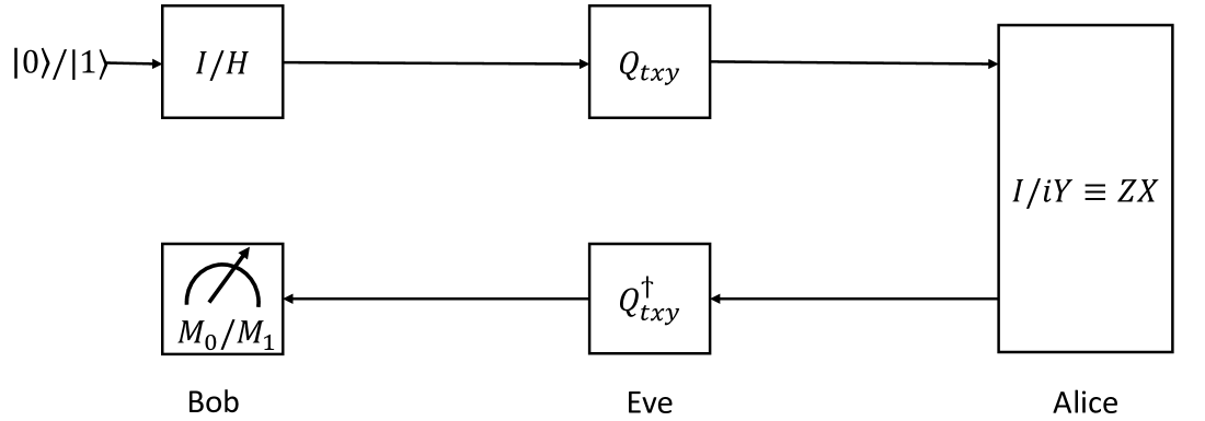In the DL04 protocol, two quantum players employ strategies to ensure secure communication. Our focus lies in determining the secure bound on QBER when accounting for the presence of an eavesdropper (Eve), who may utilize both quantum and classical attack strategies. We consider that the quantum Eve employs the following attack strategies: Wójcik’s original attack [73], Wójcik’s symmetrized attack [73] and Pavičić attack [74], denoted as $E_{1}$ , $E_{2}$ and $E_{3}$ , respectively. Additionally, there is a classical Eve employing an Intercept Resend (IR) attack strategy ( $E_{4}$ ). The detailed analysis of attack strategies is conducted in Appendices A, B, C and D. Here, we briefly describe Eve’s attack strategies to aid readers in understanding the concepts (for more details, see the Appendices). In the $E_{1}$ attack, Eve utilizes the unitary operation $Q_{txy}$ during the B-A attack and its conjugate, $Q_{txy}^{\dagger}\left(\equiv Q_{txy}^{-1}\right)$ , during the A-B attack, where $Q_{txy}(={\rm SWAP}_{tx}\,{\rm CPBS}_{txy}\,H_{y}\equiv{\rm SWAP}_{tx}\otimes I _{y}\,{\rm CPBS}_{txy}\,I_{t}\otimes I_{x}\otimes H_{y})$ . Here, A-B and B-A attack refer to Eve’s attack on the quantum channel when state transmission is from Alice to Bob and from Bob to Alice, respectively. This attack results in the state being in a higher dimensional Hilbert state with Eve’s unitary operations, leading to a higher degree of randomization through quantum superposition. This affects the final joint probabilities of Alice’s, Bob’s and Eve’s measurement outcomes as $p_{000}^{E_{1}}=q,$ $p_{001}^{E_{1}}=p_{010}^{E_{1}}=p_{011}^{E_{1}}=0,$ $p_{100}^{E_{1}}=\frac{1}{4}\left(1-q\right),$ $p_{101}^{E_{1}}=\left(1-q\right)\left(\frac{1}{4}+\frac{p}{2}\right),$ $p_{110}^{E_{1}}=0$ and $p_{111}^{E_{1}}=\frac{1}{2}\left(1-p\right)\left(1-q\right)$ . The QBER in the $E_{1}$ attack is $\frac{1}{2}\left(1-q\right)\left(1+p\right)$ and the detection probability of Eve’s presence is 0.1875. The $E_{2}$ attack is similar to the $E_{1}$ attack, with the only difference being that with a probability of $\frac{1}{2}$ , an additional unitary operation $S_{ty}$ is applied right after the operation $Q_{txy}^{-1}$ during the A-B attack. The $S_{ty}$ operation is defined as $X_{t}Z_{t}{\rm CNOT}_{ty}X_{t}$ . In this scenario, the final joint probabilities of Alice’s, Bob’s and Eve’s measurement outcomes are $p_{000}^{E_{2}}=\frac{1}{2}\left[\frac{q}{4}\left(1+p\right)+q\right]=\frac{q} {8}\left(5+p\right),$ $p_{001}^{E_{2}}=\frac{q}{8}\left(1+p\right),$ $p_{010}^{E_{2}}=p_{011}^{E_{2}}=\frac{q}{8}\left(1-p\right),$ $p_{100}^{E_{2}}=\frac{1}{4}\left(1-q\right),$ $p_{101}^{E_{2}}=\frac{1}{4}\left(1-q\right)\left(1+2p\right),$ $p_{110}^{E_{2}}=0$ and $p_{111}^{E_{2}}=\frac{1}{2}\left(1-p\right)\left(1-q\right)$ . The QBER in the $E_{2}$ attack is $\frac{1}{4}\left(2+2p-q-3pq\right)$ and the detection probability of Eve’s presence is 0.1875. In the $E_{3}$ attack, similar to the previous attacks, Eve applies the unitary operation $Q_{txy}^{\prime}$ when the photon is traveling from Bob to Alice in the B-A attack scenario. Conversely, in the A-B attack scenario, Eve applies the inverse of $Q_{txy}^{\prime}$ $\left(Q_{txy}^{\prime-1}\right)$ to the traveling photon ( $t$ ), where $Q_{txy}^{\prime}={\rm CNOT}_{ty}\left({\rm CNOT}_{tx}\otimes I_{y}\right)\left (I_{t}\otimes{\rm PBS}_{xy}\right){\rm CNOT}_{ty}\left({\rm CNOT}_{tx}\otimes I _{y}\right)\left(I_{t}\otimes H_{x}\otimes H_{y}\right)$ . In this scenario, the final joint probabilities of Alice’s, Bob’s and Eve’s measurement outcomes are $p_{000}^{E_{3}}=q,$ $p_{001}^{E_{3}}=p_{010}^{E_{3}}=p_{011}^{E_{3}}=0,$ $p_{100}^{E_{3}}=p_{101}^{E_{3}}=p_{110}^{E_{3}}=0,$ and $p_{111}^{E_{3}}=\left(1-q\right)$ . The QBER in the $E_{3}$ attack is 0 and the detection probability of Eve’s presence is 0.1875. The $E_{4}$ attack is essentially an IR attack, where the final joint probabilities of Alice’s, Bob’s, and Eve’s measurement outcomes are $p_{000}^{E_{4}}=\frac{3}{4}q,$ $p_{001}^{E_{4}}=p_{011}^{E_{4}}=0,$ $p_{010}^{E_{4}}=\frac{1}{4}q,$ $p_{100}^{E_{4}}=p_{110}^{E_{4}}=0,$ $p_{101}^{E_{4}}=\frac{1}{4}\left(1-q\right)$ and $p_{111}^{E_{4}}=\frac{3}{4}\left(1-q\right)$ . The QBER in the $E_{4}$ attack is 0.25 and the detection probability of Eve’s presence is 0.375. Before describing the conventional payoff function, it is crucial to map the DL04 protocol in a game-theoretic scenario where principles of game theory is applied into a quantum communication protocol (see Figure 1). For simplicity, we divide DL04 quantum game into different game scenarios. However, in what follows, we explain the mapping in a general context [55, 12, 75]. Let us consider game $\mathcal{G}$ as a normal form game. This game is defined as a function with an appropriate domain and range, with players’ preferences defined over the elements of the range, inducing rational strategic choices within the domain. We now describe the players’ choices in the quantum domain. In more general terms, the game $\mathcal{G}$ has a range that is equal to the output set $O$ and a domain that is the Cartesian product $S_{1}\times S_{2}\times\cdots\times S_{n}$ , where $S_{i}$ represents the set of pure strategies for the $i^{th}$ player. Each element of the domain set $S_{1}\times S_{2}\times\cdots\times S_{n}$ can be referred to as a play of game or a strategy profile. Formally, a game $\mathcal{G}$ is a function, $\mathcal{G}:S_{1}\times S_{2}\times\cdots\times S_{n}\longrightarrow O$ . In this context, $n$ represents the number of players. Since our game involves three participants, Alice, Bob and Eve. Bob’s choice of prepared state, Alice’s choice of measurement basis and Eve’s choice of attack strategy are within the domain set $S_{1}\times S_{2}\times S_{3}$ , where $S_{1},S_{2}$ and $S_{3}$ are the strategy choices of Alice, Bob and Eve, respectively. Thus, the function $\mathcal{G}$ can be specifically expressed as $\mathcal{G}:S_{1}\times S_{2}\times S_{3}\longrightarrow O$ in the form of pure strategies. Here, Bob prepares quantum states in the $Z$ or $X$ basis and sends them to Alice. For a security check, Alice measures part of Bob’s sequence and then encodes a message by performing the Pauli operation before sending it back to Bob. During this process, Eve employs various attack strategies through the quantum channel. In what follows, we elucidate how this game is incorporated into the quantum communication protocol. Alice arranges her initial sequence as a mixed state, represented by $\frac{p}{2}\left(|0\rangle\langle 0|+|1\rangle\langle 1|\right)+\frac{1-p}{2} \left(|+\rangle\langle+|+|-\rangle\langle-|\right)$ . The states of Alice resides within a 2-dimensional projective complex Hilbert space, denoted as $\mathcal{H}_{2}$ . This mixed state contains with four pure states, which can be interpreted as a superposition state within $\mathcal{H}_{2}$ . This implies that if $|0\rangle$ undergoes a projective measurement in the $X$ basis Let us assume that the process of quantum measurement in a 2-dimensional space can be characterized by the operator set { $M_{0}$ , $M_{1}$ : $M_{0}=|+\rangle\langle+|$ , $M_{1}=|-\rangle\langle-|$ }., it will collapse into $|+\rangle$ and $|-\rangle$ with a probability of $\frac{1}{2}$ . This occurrence is a result of quantum superposition. Eve also executes attacks using quantum unitary gates and ancilla states, which operate within the projective complex Hilbert space. Specifically, the Eve’s $E_{1}$ , $E_{2}$ and $E_{3}$ attacks operate within an 8-dimensional Hilbert space $\mathcal{H}_{8}$ , and the $E_{4}$ attack operates within $\mathcal{H}_{2}$ space. In our different game scenarios, we assume that Eve attacks with $E_{i}$ and $E_{j}$ with probabilities $r$ and $1-r$ , respectively. As a result of these operations by Eve, the states of Alice and Bob are further increase the quantum superposition based on the unitary operators utilized in Eve’s attacks ( inplying that the basis used by alice total number of possible outcome increases). This increase of superposition impacts the measurement outcome of the legitimate player in this game scenario The detailed descriptions of Alice’s and Bob’s unitary operations and the results of their measurements are elaborately presented in the appendices. that also increase the range of the game $\left(O\right)$ , for $O=\left\{o_{1},o_{2},o_{3}\right\}$ , $o_{1},o_{2}$ and $o_{3}$ are the output of Alice, Bob and Eve, respectively. Alice employs Pauli operations to encode the message, which also exists within $\mathcal{H}_{2}$ space. Consequently, we can describe our game as a mixed strategy game, defined as a function $\mathcal{M}$ . The 1 $-$ simplex $\Delta_{1}$ , represents the set of probability distributions over each player’s pure strategies, also known as the set of mixed strategies. Thus, our mixed strategy game $\mathcal{M}$ is defined with a domain equal to the Cartesian product of the sets of probability distributions over the pure strategies of the players. Formally, this is represented as: $$ \begin{array}[]{lcl}\mathcal{M}&:&\Delta_{1}\times\Delta_{1}\times\Delta_{1} \longrightarrow\Delta_{7}\\ \\ \mathcal{M}&:&\left(\left(p,1-p\right),\left(q,1-q\right),\left(r,1-r\right) \right)\\ &\mapsto&\left(pqr,pq\left(1-r\right),p\left(1-q\right)r,p\left(1-q\right) \left(1-r\right),\left(1-p\right)qr,\right.\\ &&\left.\left(1-p\right)q\left(1-r\right),\left(1-p\right)\left(1-q\right)r, \left(1-p\right)\left(1-q\right)\left(1-r\right)\right)\end{array}, $$ Its range includes probability distributions over the outcomes by associating these outcomes with the vertices of the 7 $-$ simplex $\Delta_{7}$ . The required projective complex Hilbert space for $\mathcal{M}$ is as follows: $$ \begin{array}[]{lcl}{\rm Bob^{\prime}s\,prepared\,state}&\longrightarrow& \mathcal{H}_{2}\\ {\rm Alice^{\prime}s\,measuremet\,basis}&\longrightarrow&\mathcal{H}_{2}\\ {\rm Alice^{\prime}s\,unitary\,operation}&\longrightarrow&\mathcal{H}_{2}\\ {\rm Eve^{\prime}s\,}E_{1},E_{2},E_{3}\,{\rm attack}&\longrightarrow&\mathcal{ H}_{8}\\ {\rm Eve^{\prime}s\,}E_{4}\,{\rm attack}&\longrightarrow&\mathcal{H}_{2}\end{ array}. $$ Additionally, we observe that the superposition states belong to Bob, along with the unitary operations executed by Alice and Eve, thus the state belongs within the higher dimensional complex Hilbert space ( $\mathcal{H}_{8}$ ). This process incorporates a higher degree of randomization via quantum superposition. The impact of such high-level randomization reflects on the outputs of the legitimate players or increase the range of this game. Accordingly, these output results influence on the key factors of the players’ payoff function, such as mutual information, QBER and the detection of Eve’s presence. Ultimately, these effects on the payoff functions determine the Nash equilibrium points for the different game scenarios. By employing quantum superposition states and quantum unitary operations, we apply non-cooperative game theory to the DL04 protocol and demonstrate that Nash equilibrium serves as a viable solution concept. Hence, we integrate gaming the quantum in our work [75, 61]. <details> <summary>x1.png Details</summary>  ### Visual Description ## Quantum Circuit Diagram: Qubit State Preparation, Transformation, and Measurement ### Overview The image displays a schematic quantum circuit diagram illustrating a sequence of operations on a qubit, involving three parties: Bob, Eve, and Alice. The diagram shows the flow of a quantum state from an initial preparation, through transformations, to a final measurement. It is a technical representation using standard quantum circuit notation with boxes representing quantum gates or operations and arrows indicating the direction of qubit flow. ### Components/Axes The diagram is structured in two horizontal rows (or "wires") representing the path of a single qubit, with components placed along them. **Top Row (Left to Right):** 1. **Initial State:** Labeled `|0⟩/|1⟩`. This represents the qubit being prepared in either the ground state `|0⟩` or the excited state `|1⟩`. 2. **First Operation Box:** A square box labeled `I/H`. This denotes a choice between the Identity gate (`I`) and the Hadamard gate (`H`). 3. **Second Operation Box:** A square box labeled `Q_xy`. This represents a specific quantum gate or operation parameterized by `x` and `y`. 4. **Arrow:** A horizontal arrow points from the `Q_xy` box to the large box on the right. **Right Side:** 5. **Large Vertical Box:** A tall rectangular box spanning both rows, labeled `I/iY ≡ ZX`. This indicates a composite operation or equivalence. `I/iY` likely represents the inverse of the Pauli-Y gate (`iY`), and `≡ ZX` states this is equivalent to the product of the Pauli-Z and Pauli-X gates. **Bottom Row (Right to Left):** 6. **Third Operation Box:** A square box labeled `Q_xy†`. The `†` symbol denotes the adjoint (or inverse) of the `Q_xy` operation from the top row. 7. **Arrow:** A horizontal arrow points from the `Q_xy†` box to the measurement box on the left. 8. **Measurement Box:** A square box containing a meter symbol (a semicircle with an arrow) and labeled `M_0/M_1`. This represents a measurement in the computational basis, yielding a classical bit result of 0 or 1. **Labels for Parties:** * **Bob:** The label "Bob" is positioned directly below the measurement box (`M_0/M_1`). * **Eve:** The label "Eve" is positioned directly below the `Q_xy†` box. * **Alice:** The label "Alice" is positioned directly below the large vertical box (`I/iY ≡ ZX`). **Flow Direction:** The arrows indicate a counter-clockwise flow: The qubit starts at the top-left (`|0⟩/|1⟩`), moves right through `I/H` and `Q_xy`, enters Alice's large operation box, then moves left along the bottom row through `Q_xy†` (Eve's operation) to the final measurement by Bob. ### Detailed Analysis * **Sequence of Operations:** 1. **State Preparation:** A qubit is initialized as `|0⟩` or `|1⟩`. 2. **Bob's Initial Gate (Top-Left):** The qubit undergoes either no operation (`I`) or a Hadamard transform (`H`), which creates a superposition state. 3. **Eve's Gate (Top-Middle):** The qubit is acted upon by the parameterized gate `Q_xy`. 4. **Alice's Gate (Right):** The qubit passes through the operation `I/iY ≡ ZX`. This is a fixed, non-parameterized gate sequence. 5. **Eve's Inverse Gate (Bottom-Middle):** The adjoint (inverse) of Eve's initial gate, `Q_xy†`, is applied. This suggests an attempt to "undo" the `Q_xy` operation. 6. **Bob's Measurement (Bottom-Left):** The final state of the qubit is measured by Bob, resulting in a classical outcome `M_0` or `M_1`. * **Mathematical Notation:** * `|0⟩`, `|1⟩`: Standard Dirac notation for quantum states. * `I`: Identity operator. * `H`: Hadamard gate. * `Q_xy`: A generic unitary operator dependent on parameters `x` and `y`. * `Q_xy†`: The Hermitian adjoint of `Q_xy`, satisfying `Q_xy * Q_xy† = I` if `Q_xy` is unitary. * `iY`: The Pauli-Y matrix multiplied by the imaginary unit `i`. * `ZX`: The product of the Pauli-Z and Pauli-X matrices. * `M_0/M_1`: Measurement outcomes corresponding to projecting onto the `|0⟩` or `|1⟩` state. ### Key Observations 1. **Symmetry and Inversion:** The circuit exhibits a symmetric structure around Alice's central operation. Eve applies `Q_xy` before Alice and its inverse `Q_xy†` after. This is a common pattern in quantum protocols for error correction, teleportation, or certain cryptographic schemes. 2. **Party Roles:** The labels assign specific roles: Alice performs a fixed, known operation. Eve performs a parameterized operation and its inverse. Bob performs the initial state manipulation (choice of `I` or `H`) and the final measurement. 3. **Equivalence Statement:** The label `I/iY ≡ ZX` inside Alice's box is a key technical detail. It asserts that the operation performed is equivalent to applying the Pauli-Z gate followed by the Pauli-X gate (or vice versa, as they anti-commute up to a phase). This is a non-trivial identity in quantum mechanics. 4. **Single Qubit Line:** The entire diagram operates on a single qubit, as indicated by the single continuous path of arrows. ### Interpretation This diagram likely represents a **quantum cryptographic protocol or a quantum computation subroutine**. The structure strongly suggests a scenario involving **decoherence-free subspaces, quantum teleportation, or a specific attack/defense model in quantum key distribution (QKD)**. * **Purpose:** The circuit tests how a specific, parameterized operation (`Q_xy` by Eve) and its inverse affect the transmission of a quantum state from Bob (as sender/measurer) through Alice's fixed channel. The final measurement by Bob reveals whether the combined operations preserved the initial state information. * **Relationships:** The operations are chained: Bob's initial choice (`I` or `H`) sets the input state for Eve's and Alice's transformations. The symmetry of `Q_xy` and `Q_xy†` implies that if Alice's operation (`I/iY`) commutes or has a specific relationship with `Q_xy`, the net effect might be identity, allowing perfect state recovery by Bob. If not, the measurement outcome will be disturbed. * **Notable Implication:** The equivalence `I/iY ≡ ZX` is crucial. In many quantum protocols, the Pauli operators (`X, Y, Z`) represent fundamental errors or basis changes. This specific equivalence might be used to model a particular type of noise or a deliberate transformation in a quantum communication channel. The diagram is a formal model for analyzing the success probability of transmitting the initial `|0⟩/|1⟩` state through this specific sequence of gates. </details> Figure 1: The circuit representation of DL04 quantum game. We will now define the payoff for each party involved. The mutual information between Alice and Bob has a positive impact on the payoffs of legitimate players (Alice and Bob), but it negatively affects Eavesdropper’s (Eve) payoff. Conversely, the mutual information shared between Alice and Eve, as well as Bob and Eve, negatively affects the payoffs of legitimate players. Additionally, legitimate players benefit from the ability to detect Eve’s presence The contribution of both parameters is equally significant, contingent upon the specific quantitative values of QBER and the detection probability of Eve’s presence ( $P_{d}$ ) observed in both message and control modes of the DL04 protocol., which improves their payoffs in this competitive scenario. On the other hand, Eve’s payoff increases with the acquisition of more information from Alice and Bob but decreases as the mutual information between Alice and Bob increases. Furthermore, Eve incurs penalties if she is detected. Consequently, Eve’s payoff is enhanced when the probability of remaining undetected is higher. Additionally, Eve may employ various quantum gates to collect information from Alice and Bob, and the greater the number of gates she uses, the more it impacts her overhead, which, in turn, adversely affects her payoff. As a result, the payoff can be customized to reflect the various scenarios and benefits of the players that we intend to analyze. The DL04 protocol, resembling a game, can be conceptualized as a zero-sum game. We may formulate the payoffs of Alice, Bob and Eve [53] for a general attack strategy $\mathcal{E}$ as follows We assume that the difficulty of preparing quantum states and performing measurement operations is the same for Alice, Bob and Eve. Therefore, we do not factor in this contribution when estimating the payoffs for these parties., $$ \begin{array}[]{lcl}P_{A}^{\mathcal{E}}(p,q)&=&\omega_{a}I\left({\rm A,B} \right)-\omega_{b}I\left({\rm A,E}\right)-\omega_{c}I\left({\rm B,E}\right)+ \omega_{d}\left(\frac{P_{d}+{\rm QBER}}{2}\right)\\ \\ P_{B}^{\mathcal{E}}(p,q)&=&\omega_{a}I\left({\rm A,B}\right)-\omega_{c}I\left( {\rm A,E}\right)-\omega_{b}I\left({\rm B,E}\right)+\omega_{d}\left(\frac{P_{d} +{\rm QBER}}{2}\right)\\ \\ P_{E}^{\mathcal{E}}(p,q)&=&-\omega_{e}I\left({\rm A,B}\right)+\omega_{f}I\left ({\rm A,E}\right)+\omega_{g}I\left({\rm B,E}\right)+\omega_{h}\left(1-\frac{P_ {d}+{\rm QBER}}{2}\right)-\omega_{i}n_{1}-\omega_{j}n_{2}-\omega_{k}n_{3}\end{ array}, \tag{1} $$ where $\omega_{a},\,\omega_{b},\,\omega_{c},\,\omega_{d},\,\omega_{e},\,\omega_{f},\, \omega_{g},\,\omega_{h},\,\omega_{i},\,\omega_{j}$ and $\omega_{k}$ are all positive real numbers, and they are interpreted as the factors or weights assigned to each component within the payoff such that $\stackrel{{\scriptstyle[}}{{m}}=a]{d}{\sum}\omega_{m}=1$ and $\stackrel{{\scriptstyle[}}{{n}}=e]{k}{\sum}\omega_{n}=1$ where $m\in\{a,b,c,d\}$ and $n\in\{e,f,\ldots,k\}$ . Further, $I\left({\rm A,B}\right)$ , $I\left({\rm A,E}\right)$ and $I\left({\rm B},{\rm E}\right)$ are the mutual information between Alice and Bob, Alice and Eve and Bob and Eve, respectively. Here, $P_{d}$ is the probability of detection of Eve’s presence, $n_{1}$ , $n_{2}$ and $n_{3}$ are the number of single-qubit, two-qubit and three-qubit gates, respectively. Here, it may be noted that in the payoff function described above, $P_{d}$ and $QBER$ are considered on equal footing because both $P_{d}$ and $QBER$ reveal the presence of Eve with a similar effect. Assuming Eve has unlimited quantum resources and perfect quantum gates, we can set $\omega_{i}=\omega_{j}=\omega_{k}=0$ . This implies she can use as many quantum gates as needed for her attack without negatively impacting her payoff function. To simplify the analysis, in what follows we have considered the effect of each component in the payoff is the same. Thus, in our consideration, $\omega_{a}=\omega_{b}=\omega_{c}=\omega_{d}=\omega_{e}=\omega_{f}=\omega_{g}= \omega_{h}=0.25$ . The Eq. (1) is modified as, $$ \begin{array}[]{lcl}P_{A}^{\mathcal{E}}(p,q)&=&0.25\times\left[I\left({\rm A,B }\right)-I\left({\rm A,E}\right)-I\left({\rm B,E}\right)+\left(\frac{P_{d}+{ \rm QBER}}{2}\right)\right]\\ \\ P_{B}^{\mathcal{E}}(p,q)&=&0.25\times\left[I\left({\rm A,B}\right)-I\left({\rm A ,E}\right)-I\left({\rm B,E}\right)+\left(\frac{P_{d}+{\rm QBER}}{2}\right) \right]\\ \\ P_{E}^{\mathcal{E}}(p,q)&=&0.25\times\left[-I\left({\rm A,B}\right)+I\left({ \rm A,E}\right)+I\left({\rm B,E}\right)+\left(1-\frac{P_{d}+{\rm QBER}}{2} \right)\right]\end{array}. \tag{2} $$ In this context, it is evident that the payoffs for Alice and Bob, as denoted by Eq. (2), are identical. For our subsequent analysis, we will treat these individual payoffs independently. This approach is taken due to the distinct probabilities, represented by $q$ for Alice and $p$ for Bob, pertaining to the selection of encoded bit values and the utilization of the $Z$ basis to prepare initial states. This is illustrated more clearly in the tabular format of the game $\mathcal{M}$ in Table 1. | Alice $0\left(q\right)$ | $\left(rP_{A}^{E_{i}}\left(p,q\right)+\left(1-r\right)P_{A}^{E_{j}}\left(p,q \right),\right.$ $\left.rP_{B}^{E_{i}}\left(p,q\right)+\left(1-r\right)P_{B}^{E_{j}}\left(p,q \right),P_{E}^{E_{i/j}}\left(p,q\right)\right)$ | $Z\left(p\right)$ | | $\left(rP_{A}^{E_{i}}\left(1-p,q\right)+\left(1-r\right)P_{A}^{E_{j}}\left(1-p, q\right),rP_{B}^{E_{i}}\left(1-p,q\right)\right.$ $\left.+\left(1-r\right)P_{B}^{E_{j}}\left(1-p,q\right),P_{E}^{E_{i/j}}\left(1- p,q\right)\right)$ | $X\left(1-p\right)$ | | --- | --- | --- | --- | --- | --- | | $1\left(1-q\right)$ | $\left(rP_{A}^{E_{i}}\left(p,1-q\right)+\left(1-r\right)P_{A}^{E_{j}}\left(p,1- q\right),\right.$ | | | $\left(rP_{A}^{E_{i}}\left(1-p,1-q\right)+\left(1-r\right)P_{A}^{E_{j}}\left(1- p,1-q\right),\right.$ | | | $rP_{B}^{E_{i}}\left(p,1-q\right)+\left(1-r\right)P_{B}^{E_{j}}\left(p,1-q \right),$ | | | $rP_{B}^{E_{i}}\left(1-p,1-q\right)+\left(1-r\right)P_{B}^{E_{j}}\left(1-p,1-q \right),$ | | | | $\left.P_{E}^{E_{i/j}}\left(p,1-q\right)\right)$ | | | $\left.P_{E}^{E_{i/j}}\left(1-p,1-q\right)\right)$ | | | Table 1: Payoff matrix for the $\mathcal{M}$ game. The first, second and third entry in the parenthesis denotes the payoff of Alice, Bob and Eve. Here, $r$ and $1-r$ denote the probabilities assigned to the selection of attacks $E_{i}$ and $E_{j}$ by an eavesdropper, Eve, respectively. ## III Investigating Threshold Bound of QBER using Nash Equilibrium A Nash equilibrium is a set of actions in a game where no player can improve their expected outcome (payoff) by altering their choice unilaterally, assuming the other players’ decisions remain unchanged. In a generalized concept of Nash equilibrium that represents a stochastic steady state of a strategic game, each player has the option to select a probability distribution over their available actions instead of being limited to a single, fixed choice. This probability distribution is referred to as a mixed strategy. In a well-defined game, it is generally assumed that all participants act logically and rationally. As a result, the primary goal for all players is to optimize (maximize in our case ) their expected payoffs. For simplicity, we evaluate mixed strategy Nash equilibrium A mixed strategy Nash equilibrium in a normal-form game is a set of mixed strategies for each player, where no player has an incentive to unilaterally deviate given the strategies chosen by others, ensuring mutual optimality. by taking three sets of game scenarios $E_{1}$ - $E_{2}$ , $E_{1}$ - $E_{3}$ and $E_{2}$ - $E_{3}$ scenario where each player is looking to play a mixed quantum strategy that makes her opponent indifferent between her pure quantum strategies All payoff elements for all parties under the attack scenarios $E_{1}$ , $E_{2}$ , $E_{3}$ and $E_{4}$ are computed in Appendices A, B, C and D, respectively.. Based on this assumption, we can compare the results derived from Nash equilibrium points to obtain the secure bound of QBER (see Appendix E). Firstly, we elucidate the best response function and subsequently apply it to various game scenarios. For each game scenario, we will establish the best response function for each party. The best response for an individual is defined as the probability of choosing their rational choice in a mixed strategy scenario, aiming to achieve the best utility when other parties make their decisions independently and arbitrarily. Let’s consider the best response function for Alice in the game $E_{i}$ - $E_{j}$ . Suppose Alice has the probability $q$ of choosing her classical bit information when Bob and Eve independently choose their decisions with probabilities $p$ and Here, $r$ and $1-r$ denote the probabilities assigned to the selection of attacks $E_{i}$ and $E_{j}$ by an eavesdropper, Eve, respectively. $r$ . For the pure strategy best response function of Alice, denoted as $q=1$ and $q=0$ , it can be expressed as [76]: $$ B_{A}\left(p,r\right)\coloneqq rP_{A}^{E_{i}}\left(p,1\right)+\left(1-r\right) P_{A}^{E_{j}}\left(p,1\right)>rP_{A}^{E_{i}}\left(p,0\right)+\left(1-r\right)P _{A}^{E_{j}}\left(p,0\right). $$ and $$ B_{A}\left(p,r\right)\coloneqq rP_{A}^{E_{i}}\left(p,1\right)+\left(1-r\right) P_{A}^{E_{j}}\left(p,1\right)<rP_{A}^{E_{i}}\left(p,0\right)+\left(1-r\right)P _{A}^{E_{j}}\left(p,0\right), $$ respectively. For the mixed strategy best response function of Alice, is given by: $$ B_{A}\left(p,r\right)\coloneqq rP_{A}^{E_{i}}\left(p,1\right)+\left(1-r\right) P_{A}^{E_{j}}\left(p,1\right)=rP_{A}^{E_{i}}\left(p,0\right)+\left(1-r\right)P _{A}^{E_{j}}\left(p,0\right). $$ Using the definition of the best response function, we can similarly define the best response functions for Bob and Eve as $B_{B}\left(q,r\right)$ and $B_{E}\left(p,q\right)$ , where Bob and Eve assign their probabilities $p$ and $r$ with best responses to $q,r$ and $p,q$ , respectively. $E_{1}$ - $E_{2}$ game scenario Previously defined probabilities $p$ and $q$ can be used. Let’s assume that Eve chooses the $E_{1}$ ( $E_{2}$ ) attack with probability $r$ ( $1-r$ ). We denote the best response function of Alice as $B_{A}\left(p,r\right)$ , which represents the set of probabilities that Alice assigns to choosing the Z basis in her best responses to $p$ and $r$ [76]. Similarly, the best response functions for Bob and Eve are $B_{B}\left(q,r\right)$ and $B_{E}\left(p,q\right)$ , respectively. We have, $$ \begin{array}[]{lcl}B_{A}\left(p,r\right)&=&\begin{cases}\left\{q=1\right\}&{ \rm if}\,\,rP_{A}^{E_{1}}\left(p,1\right)+\left(1-r\right)P_{A}^{E_{2}}\left(p ,1\right)>rP_{A}^{E_{1}}\left(p,0\right)+\left(1-r\right)P_{A}^{E_{2}}\left(p, 0\right)\\ \left\{q:0\leq q\leq 1\right\}&{\rm if}\,\,rP_{A}^{E_{1}}\left(p,1\right)+ \left(1-r\right)P_{A}^{E_{2}}\left(p,1\right)=rP_{A}^{E_{1}}\left(p,0\right)+ \left(1-r\right)P_{A}^{E_{2}}\left(p,0\right)\\ \left\{q=0\right\}&{\rm if}\,\,rP_{A}^{E_{1}}\left(p,1\right)+\left(1-r\right) P_{A}^{E_{2}}\left(p,1\right)<rP_{A}^{E_{1}}\left(p,0\right)+\left(1-r\right)P _{A}^{E_{2}}\left(p,0\right)\end{cases}\\ \\ B_{B}\left(q,r\right)&=&\begin{cases}\left\{p=1\right\}&{\rm if}\,\,rP_{B}^{E_ {1}}\left(1,q\right)+\left(1-r\right)P_{B}^{E_{2}}\left(1,q\right)>rP_{B}^{E_{ 1}}\left(0,q\right)+\left(1-r\right)P_{B}^{E_{2}}\left(0,q\right)\\ \left\{p:0\leq p\leq 1\right\}&{\rm if}\,\,rP_{B}^{E_{1}}\left(1,q\right)+ \left(1-r\right)P_{B}^{E_{2}}\left(1,q\right)=rP_{B}^{E_{1}}\left(0,q\right)+ \left(1-r\right)P_{B}^{E_{2}}\left(0,q\right)\\ \left\{p=0\right\}&{\rm if}\,\,rP_{B}^{E_{1}}\left(1,q\right)+\left(1-r\right) P_{B}^{E_{2}}\left(1,q\right)<rP_{B}^{E_{1}}\left(0,q\right)+\left(1-r\right)P _{B}^{E_{2}}\left(0,q\right)\end{cases}\\ \\ B_{E}\left(p,q\right)&=&\begin{cases}\left\{r=1\right\}&{\rm if}\,\,P_{E}^{E_{ 1}}\left(p,q\right)>P_{E}^{E_{2}}\left(p,q\right)\\ \left\{r:0\leq r\leq 1\right\}&{\rm if}\,\,P_{E}^{E_{1}}\left(p,q\right)=P_{E} ^{E_{2}}\left(p,q\right)\\ \left\{r=0\right\}&{\rm if}\,\,P_{E}^{E_{1}}\left(p,q\right)<P_{E}^{E_{2}} \left(p,q\right)\end{cases}\end{array}. \tag{3} $$ The best response functions for Alice, Bob and Eve in the game scenarios $E_{1}$ - $E_{3}$ and $E_{2}$ - $E_{3}$ are as follows, $$ \begin{array}[]{lcl}B_{A}\left(p,r\right)&=&\begin{cases}\left\{q=1\right\}&{ \rm if}\,\,rP_{A}^{E_{1}}\left(p,1\right)+\left(1-r\right)P_{A}^{E_{3}}\left(p ,1\right)>rP_{A}^{E_{1}}\left(p,0\right)+\left(1-r\right)P_{A}^{E_{3}}\left(p, 0\right)\\ \left\{q:0\leq q\leq 1\right\}&{\rm if}\,\,rP_{A}^{E_{1}}\left(p,1\right)+ \left(1-r\right)P_{A}^{E_{3}}\left(p,1\right)=rP_{A}^{E_{1}}\left(p,0\right)+ \left(1-r\right)P_{A}^{E_{3}}\left(p,0\right)\\ \left\{q=0\right\}&{\rm if}\,\,rP_{A}^{E_{1}}\left(p,1\right)+\left(1-r\right) P_{A}^{E_{3}}\left(p,1\right)<rP_{A}^{E_{1}}\left(p,0\right)+\left(1-r\right)P _{A}^{E_{3}}\left(p,0\right)\end{cases}\\ \\ B_{B}\left(q,r\right)&=&\begin{cases}\left\{p=1\right\}&{\rm if}\,\,rP_{B}^{E_ {1}}\left(1,q\right)+\left(1-r\right)P_{B}^{E_{3}}\left(1,q\right)>rP_{B}^{E_{ 1}}\left(0,q\right)+\left(1-r\right)P_{B}^{E_{3}}\left(0,q\right)\\ \left\{p:0\leq p\leq 1\right\}&{\rm if}\,\,rP_{B}^{E_{1}}\left(1,q\right)+ \left(1-r\right)P_{B}^{E_{3}}\left(1,q\right)=rP_{B}^{E_{1}}\left(0,q\right)+ \left(1-r\right)P_{B}^{E_{3}}\left(0,q\right)\\ \left\{p=0\right\}&{\rm if}\,\,rP_{B}^{E_{1}}\left(1,q\right)+\left(1-r\right) P_{B}^{E_{3}}\left(1,q\right)<rP_{B}^{E_{1}}\left(0,q\right)+\left(1-r\right)P _{B}^{E_{3}}\left(0,q\right)\end{cases}\\ \\ B_{E}\left(p,q\right)&=&\begin{cases}\left\{r=1\right\}&{\rm if}\,\,P_{E}^{E_{ 1}}\left(p,q\right)>P_{E}^{E_{3}}\left(p,q\right)\\ \left\{r:0\leq r\leq 1\right\}&{\rm if}\,\,P_{E}^{E_{1}}\left(p,q\right)=P_{E} ^{E_{3}}\left(p,q\right)\\ \left\{r=0\right\}&{\rm if}\,\,P_{E}^{E_{1}}\left(p,q\right)<P_{E}^{E_{3}} \left(p,q\right)\end{cases}\end{array}. \tag{4} $$ and $$ \begin{array}[]{lcl}B_{A}\left(p,r\right)&=&\begin{cases}\left\{q=1\right\}&{ \rm if}\,\,rP_{A}^{E_{2}}\left(p,1\right)+\left(1-r\right)P_{A}^{E_{3}}\left(p ,1\right)>rP_{A}^{E_{2}}\left(p,0\right)+\left(1-r\right)P_{A}^{E_{3}}\left(p, 0\right)\\ \left\{q:0\leq q\leq 1\right\}&{\rm if}\,\,rP_{A}^{E_{2}}\left(p,1\right)+ \left(1-r\right)P_{A}^{E_{3}}\left(p,1\right)=rP_{A}^{E_{2}}\left(p,0\right)+ \left(1-r\right)P_{A}^{E_{3}}\left(p,0\right)\\ \left\{q=0\right\}&{\rm if}\,\,rP_{A}^{E_{2}}\left(p,1\right)+\left(1-r\right) P_{A}^{E_{3}}\left(p,1\right)<rP_{A}^{E_{2}}\left(p,0\right)+\left(1-r\right)P _{A}^{E_{3}}\left(p,0\right)\end{cases}\\ \\ B_{B}\left(q,r\right)&=&\begin{cases}\left\{p=1\right\}&{\rm if}\,\,rP_{B}^{E_ {2}}\left(1,q\right)+\left(1-r\right)P_{B}^{E_{3}}\left(1,q\right)>rP_{B}^{E_{ 2}}\left(0,q\right)+\left(1-r\right)P_{B}^{E_{3}}\left(0,q\right)\\ \left\{p:0\leq p\leq 1\right\}&{\rm if}\,\,rP_{B}^{E_{2}}\left(1,q\right)+ \left(1-r\right)P_{B}^{E_{3}}\left(1,q\right)=rP_{B}^{E_{2}}\left(0,q\right)+ \left(1-r\right)P_{B}^{E_{3}}\left(0,q\right)\\ \left\{p=0\right\}&{\rm if}\,\,rP_{B}^{E_{2}}\left(1,q\right)+\left(1-r\right) P_{B}^{E_{3}}\left(1,q\right)<rP_{B}^{E_{2}}\left(0,q\right)+\left(1-r\right)P _{B}^{E_{3}}\left(0,q\right)\end{cases}\\ \\ B_{E}\left(p,q\right)&=&\begin{cases}\left\{r=1\right\}&{\rm if}\,\,P_{E}^{E_{ 2}}\left(p,q\right)>P_{E}^{E_{3}}\left(p,q\right)\\ \left\{r:0\leq r\leq 1\right\}&{\rm if}\,\,P_{E}^{E_{2}}\left(p,q\right)=P_{E} ^{E_{3}}\left(p,q\right)\\ \left\{r=0\right\}&{\rm if}\,\,P_{E}^{E_{2}}\left(p,q\right)<P_{E}^{E_{3}} \left(p,q\right)\end{cases}\end{array}. 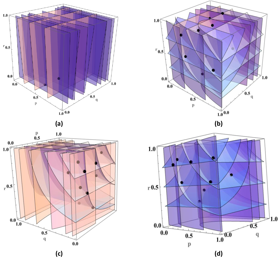\tag{5} $$ In the context of a quantum game, Figure 2 shows the best response functions for different game scenarios. These functions represent each player’s optimal strategy in response to the strategies of the other players. The mixed strategy Nash equilibrium is found at the points where these best response functions intersect. This means that at these intersections, each player’s strategy is optimal given the strategies of the others. It is important to note that there can be multiple intersection points, each corresponding to different game scenarios. These points of intersection indicate the Nash equilibrium for each player in these game scenarios. In subfigures (a), (b), (c) and (d) of Figure 2, we identify the Nash equilibrium points for the $E_{1}$ - $E_{2}$ , $E_{1}$ - $E_{3}$ , $E_{2}$ - $E_{3}$ and $E_{1}$ - $E_{4}$ game scenarios, respectively. Each subfigure depicts three different curves, each representing the best response function of a player within the mixed quantum strategy game. These curves show the optimal strategies for each player in response to the others. The intersection points of these three curves indicate the most stable points in each game scenario. From these intersections, we can determine the most stable probability distributions in the mixed quantum strategy game, which are optimal for all players. We provide a summary of this data, including the payoffs of each player, in Table 2 in Appendix E. In the provided summary, we analyze our mixed strategy Nash equilibrium points for different game scenarios and investigate the secure QBER bound. In the context of Eq. (2), it becomes evident that the payoff functions for the three parties depend on the variables $p,q$ ( $q$ ) for Eve’s attack strategies, $E_{1}$ , $E_{2}$ ( $E_{3}$ , $E_{4}$ ). Furthermore, our game can be represented as a normal form game (strategic form game) because players have no information at their decision points about other players’ choices when making their moves. In this setup, all parties independently select their strategies. Specifically, Bob selects the $Z$ basis with a probability of $p$ , Eve chooses the attack strategy with a probability of $r$ , and Alice, in message mode, selects the encoded bit $0 0$ with a probability of $q$ . In our analysis, both Alice and Bob share the same payoff functions (2)). In the $E_{1}$ - $E_{2}$ game scenario, the expected payoffs for Alice/Bob and Eve are given by $rP_{A/B}^{E_{1}}(p,q)+(1-r)P_{A/B}^{E_{2}}(p,q)$ and $rP_{E}^{E_{1}}(p,q)+(1-r)P_{E}^{E_{2}}(p,q)$ , respectively. By comparing the payoff differences between Eve and Alice (see in Table 2), we can identify among the Nash equilibrium points where Eve or Alice/Bob benefit the most. In the $E_{1}$ - $E_{2}$ game scenario, Eve benefits individually at the Nash equilibrium point $(0.45,0.195,0.005)$ , while Alice/Bob benefits individually at the Nash equilibrium point $(0.72,0.208,0.225)$ . Similarly, in the $E_{1}$ - $E_{3}$ game scenario, Eve and Alice/Bob benefit individually at Nash equilibrium points $\left(0.41,0.39,0.412\right)$ and $\left(0.84,0.047,0.525\right)$ , respectively. In the $E_{2}$ - $E_{3}$ game scenario, Eve and Alice/Bob benefit individually at Nash equilibrium points $\left(0.385,0.215,0.262\right)$ and $\left(0.80,0.115,0.885\right)$ , respectively. In conclusion, there is no Pareto optimal Nash equilibrium point in our game scenarios where payoffs would be favorable to the entire group of players. We calculate the QBER for all Nash equilibrium points in different game scenarios. It is pertinent to highlight that the expected QBER value for the $E_{i}$ - $E_{j}$ game scenario is defined as $\epsilon_{E_{i}-E_{2}}=r\,{\rm QBER}_{E_{i}}+\left(1-r\right){\rm QBER}_{E_{j}}$ , where $r$ is a probability of Eve’s choice to perform $E_{i}$ attack. In any given game scenario, Eve’s optimal scenario is characterized by either the maximum payoff difference (the discrepancy between Eve’s and Alice’s payoffs) or the minimum QBER. Our objective is to determine the QBER threshold value. Consequently, we seek the minimum QBER values across all game scenarios outlined in Table 2. These values correspond to the Nash equilibrium points, representing situations where Eve is strategically positioned to conceal her presence most effectively. The minimum QBER values at Nash equilibrium points are $0.610303$ , $0.152451$ and $0.143882$ for the $E_{1}$ - $E_{2}$ , $E_{1}$ - $E_{3}$ and $E_{2}$ - $E_{3}$ game scenarios, respectively. The reduction in the minimum QBER value Considering lower QBER value empower Eve the most, that bound gives the most secure condition on a quantum protocol. (in message mode) suggests that more potent attack strategies by Eve are being applied in this game scenario when the minimum or same $P_{d}$ (detection probability of Eve’s presence in control mode) is achieved for the attacks within this game scenario. These lower QBER values are designed to identify more sophisticated quantum attacks by Eve within the game-like scenario. Following an analysis of the threshold values of QBER, we conclude that $E_{3}$ represents the most powerful quantum attack, followed by $E_{2}$ , and then $E_{1}$ . This implies that whenever Eve employs a powerful attack, she attains a higher payoff, posing a threat to both Alice and Bob. To address this threat in our DL04 protocol game scenario, we set a lower minimum value for the QBER corresponding to this specific potent attack by Eve. The threshold is determined by evaluating all Nash equilibrium points within these game scenarios that encompass the mentioned attack. As previously noted, a player with limited access to quantum resources appears to be a classical player. In our analysis, the $E_{4}$ attack is considered a classical attack by Eve, implying she is a classical eavesdropper when performing the $E_{4}$ attack. We also compare the classical attack $E_{4}$ with the simplest quantum attack, $E_{1}$ . Furthermore, we analyze the $E_{4}$ attack (IR attack) in comparison with the $E_{1}$ attack as a $E_{1}$ - $E_{4}$ game scenario. In this game scenario, the minimum value of QBER is found to be $0.323478$ , which is lower than $E_{1}$ - $E_{2}$ game scenario. Despite this fact, $E_{4}$ is considered a less powerful attack than $E_{1}$ because the $P_{d}$ value is higher for $E_{4}$ (37.5%) compared to that for $E_{1}$ (18.75%) in control mode. To determine the secure upper bound of the QBER, denoted as $\epsilon$ , considering all attack scenarios in the entire game, we focus on this game scenario involving potent attacks which is the $E_{2}$ - $E_{3}$ game scenario. In this context, the upper bound of QBER is found to be $\epsilon=0.143882$ because this is the minimum QBER value for the game scenario where the most potent attack $E_{3}$ is present. The lower bound of QBER is $0 0$ because if Eve applies only the $E_{3}$ attack, no error will be detected in message mode (see Appendix C). Furthermore, the lower and upper bounds of the detection probability of Eve’s presence ( $P_{d}$ ) in control mode are established at $0.1875$ and $0.375$ , respectively. Consequently, we can deduce that the DL04 protocol demonstrates $\epsilon$ -secure, under the set of collective and individual (IR) attacks, denoted as $E_{1}$ , $E_{2}$ , $E_{3}$ and $E_{4}$ . <details> <summary>x2.png Details</summary>  ### Visual Description \n ## 3D Surface Plots in a Unit Cube ### Overview The image displays four separate 3D plots, labeled (a), (b), (c), and (d), arranged in a 2x2 grid. Each plot visualizes semi-transparent, colored surfaces and scattered black data points within a cubic domain defined by three axes: `p`, `q`, and `r`. All axes range from 0.0 to 1.0. The plots appear to be generated by mathematical software (e.g., Mathematica, MATLAB) and likely represent different functions, manifolds, or solution sets within a unit cube. ### Components/Axes * **Axes Labels:** Each plot has three axes labeled `p`, `q`, and `r`. * **Axis Scales:** All axes are linear and span the interval [0.0, 1.0]. Tick marks are visible at 0.0, 0.5, and 1.0. * **Subplot Labels:** Each plot is identified by a lowercase letter in parentheses: `(a)`, `(b)`, `(c)`, `(d)`, placed directly below its respective cube. * **Visual Elements:** * **Surfaces:** Multiple semi-transparent, colored surfaces are plotted within each cube. Colors include shades of purple, blue, and pink/peach. The surfaces vary in shape from planar to complexly curved. * **Data Points:** Solid black spheres (points) are scattered within the volume of each cube. Their number and distribution differ per plot. * **Legend:** There is no explicit legend provided. The meaning of the different surface colors and the data points is not defined within the image itself. ### Detailed Analysis **Subplot (a):** * **Surface Geometry:** The surfaces appear as a series of parallel, vertical planes. They are oriented perpendicular to the `p`-axis, meaning they represent constant values of `p`. The planes are spaced at regular intervals along the `p`-axis. * **Surface Color:** The planes are colored in a gradient from light pink/peach (near `p=0`) to dark purple (near `p=1`). * **Data Points:** Two black data points are visible. One is located near the center of the cube (approximately `p=0.5, q=0.5, r=0.5`). The second is positioned lower and closer to the front face (approximately `p=0.7, q=0.3, r=0.2`). **Subplot (b):** * **Surface Geometry:** The surfaces are complex, intersecting, and curved. They do not align with constant coordinate planes. The shapes suggest they could be level sets of a multivariate function or solutions to a system of equations. * **Surface Color:** The surfaces are predominantly shades of purple and blue, with some pinkish hues visible where surfaces overlap or are viewed edge-on. * **Data Points:** Approximately 10-12 black data points are scattered throughout the volume. They do not appear to lie on the visible surfaces. Their distribution seems somewhat random, with a slight clustering in the upper half of the cube (higher `r` values). **Subplot (c):** * **Surface Geometry:** The surfaces are curved and appear to "drape" from the top face (`r=1`) of the cube downwards. They are not closed shapes but rather open sheets. The curvature is more pronounced along the `q` and `r` dimensions. * **Surface Color:** The surfaces are primarily light pink/peach, with some purple/blue areas where they intersect or are viewed from a different angle. * **Data Points:** Approximately 8-10 black data points are visible. They are mostly located in the central region of the cube, seemingly "caught" between or near the draped surfaces. **Subplot (d):** * **Surface Geometry:** This plot features a prominent, central, bowl-shaped or saddle-shaped surface that is open at the top. Additional, more planar surfaces intersect this central shape. * **Surface Color:** The central curved surface is a distinct blue. The intersecting planar surfaces are shades of purple. * **Data Points:** Approximately 7-9 black data points are present. They are distributed around the central blue surface, with several points appearing to lie on or very close to the purple planar surfaces. ### Key Observations 1. **Progression of Complexity:** There is a clear visual progression from the simple, planar geometry in (a) to the increasingly complex, curved, and intersecting geometries in (b), (c), and (d). 2. **Point-Surface Relationship:** The relationship between the black data points and the colored surfaces varies. In (a), points are isolated from the planes. In (c) and (d), points appear more associated with the surfaces, potentially lying on them or in their vicinity. 3. **Color Consistency:** While the specific meaning is unknown, the color palette (purple, blue, pink) is used consistently across all four subplots, suggesting they may represent related mathematical entities or parameters. 4. **Viewpoint:** All four cubes are viewed from the same isometric perspective, with the origin (`p=0, q=0, r=0`) at the bottom-left-rear corner. This allows for direct visual comparison of the geometries. ### Interpretation The image likely illustrates different scenarios or solutions within a three-parameter space (`p`, `q`, `r`), common in fields like optimization, statistical mechanics, game theory, or control systems. * **What the data suggests:** The plots demonstrate how the structure of a solution set (the colored surfaces) and the location of specific points of interest (the black dots) can change dramatically under different conditions or for different functions. * **Plot (a)** could represent a simple, decoupled system where one variable (`p`) is independent, creating planar constraints. * **Plots (b), (c), and (d)** show increasingly coupled and nonlinear relationships between the variables, resulting in complex manifolds. * **How elements relate:** The black points are likely specific samples, optima, equilibria, or initial conditions being studied in relation to the broader solution landscape defined by the surfaces. Their placement relative to the surfaces is the key piece of information. * **Notable patterns/anomalies:** The most striking pattern is the transformation of the surface topology. The transition from parallel planes to a complex, interconnected web of curved sheets indicates a fundamental change in the underlying mathematical model. The consistent use of color implies a categorical distinction (e.g., different constraint types, energy levels, or probability thresholds) that is not labeled but is maintained across all visualizations. **In summary, this figure is a technical visualization comparing four distinct 3D manifolds within a unit cube, each populated with a set of data points. It serves to contrast the geometric complexity and point distribution across different models or parameter sets.** </details> Figure 2: (Color online) The plot shows Nash equilibrium points where the best response functions of the three players intersect in our mixed strategy game scenario. The low-density layer, medium-density layer, and high-density layer correspond to the best response functions of Alice, Bob, and Eve, respectively: (a) $E_{1}$ - $E_{2}$ game scenario, (b) $E_{1}$ - $E_{3}$ game scenario, (c) $E_{2}$ - $E_{3}$ game scenario, (d) $E_{1}$ - $E_{4}$ game scenario. ## IV Discussion In this paper, we propose a new security definition for quantum communication protocols in the context of collective attacks and IR attack using Nash equilibrium. Alternatively, this can be viewed as a game-theoretic security bound against collective attacks using Nash equilibrium. Nash equilibrium points are stable points that provide rational probabilities for decision-making in a mixed quantum strategy game. These probabilities create a stable game situation for all parties, enabling the evaluation of cryptographic parameters such as the threshold value of QBER. In a real-world scenario where decisions are made independently by all parties, achieving a stable point is less likely and may lead to a more unstable situation. Therefore, the identification of the lowest QBER value from the stable game scenario establishes a secure threshold boundary for the realistic implementation of the quantum protocol. Our analysis illustrates that the security (denoted as $\epsilon$ -secure) of any quantum communication protocol depends on the choices of attack strategies employed by the eavesdropper, Eve. A smaller value of $\epsilon$ indicates a more potent attack strategy by Eve. Furthermore, our findings suggest that a quantum Eve possesses greater power than a classical Eve Ensuring that Eve’s selection of unitary operation and the execution of the measurement operation are appropriately synchronized within the quantum operation.. In our investigation, we assume that Eve has unlimited quantum resources, leading us to neglect the last three terms of Eve’s payoff in Eq. (1). To simplify our analysis, we also assume equal contributions of all payoff elements for each party, with weighted values set at $\frac{1}{4}$ . We divide our game into four different game scenarios and determine the Nash equilibrium points for each game scenario. Subsequently, we identify the minimum value of QBER within each game scenario, which corresponds to the secure bound of QBER for that specific game scenario. Finally, we determine the threshold bound of QBER ( $\epsilon$ ) for the entire game by evaluating the minimum QBER value within the game scenario that encompasses the most potent attacks. Moreover, it has been observed that the DL04 protocol is vulnerable to Pavičić attacks in message mode due to the QBER being $0 0$ . In this scenario, security is ensured through the control mode executed jointly by both legitimate parties. However, the security concern for this attack will be mitigated through the control mode. It is noteworthy that quantum communication protocols serve various purposes, with security sometimes prioritized over efficiency, and vice versa. To address such trade-off scenarios, one may generalize our analysis by introducing $\omega_{i},\,\omega_{j},\,\omega_{k}\neq 0$ , and $\omega_{m}\neq\omega_{n}$ if $m\neq n$ . This implies distinct weighted values with each payoff, with the sum normalized to $1$ (ensuring weights assigned to players are normalized). Assuming $\omega_{i},\,\omega_{j},\,\omega_{k}\neq 0$ , Eq. (1) yields $n_{1}=1$ , $n_{2}=1$ , $n_{3}=1$ for $E_{1}$ , $n_{1}=4$ , $n_{2}=2$ , $n_{3}=1$ for $E_{2}$ , $n_{1}=2$ , $n_{2}=5$ , $n_{3}=0$ for $E_{3}$ and $n_{1}=2$ , $n_{2}=n_{3}=0$ for $E_{4}$ attack strategies. It is important to note that the cost of using multi-qubit gates goes up as the number of qubits in the gate increases. Importantly, our approach can be further generalized to encompass an entire game-like scenario with all these attacks together rather than a set of different game scenarios. Under this assumption, different probabilities would exist for applying various attacks by eavesdroppers, leading to the identification of Pareto optimal Nash equilibrium points under specific conditions. Consequently, the expression for the QBER bound ( $\epsilon$ ) becomes dependent on these generalized parameters. Our methodology for establishing the securely bounded threshold of QBER is employed in the DL04 protocol. This approach is adaptable to both existing and future protocols, allowing for the attainment of diverse information theoretic bounds. This flexibility accommodates various strategies implemented by stakeholders and aligns with the purpose of applying quantum protocols. We defer further investigation to integrate additional game-theoretic features suitable for various purposes in different quantum protocols, considering other attributes of quantum mechanics. This collaborative effort aims to yield more robust results, enhancing the analysis of quantum information bounds. ### Acknowledgment: Authors acknowledge support from the QUEST scheme of the Interdisciplinary Cyber-Physical Systems (ICPS) program of the Department of Science and Technology (DST), India, Grant No.: DST/ICPS/QuST/Theme-1/2019/14 (Q80). They also thank R. Srikanth for his interest and useful technical feedback on this work. ## Availability of data and materials No additional data is needed for this work. ## Competing interests The authors declare that they have no competing interests. ## References - Gibbons [1992] R. S. Gibbons, Game theory for applied economists (Princeton University Press: Princeton, NJ, USA, 1992; ISBN 978-0-691-00395-5, 1992). - Ordeshook et al. [1986] P. C. Ordeshook et al., Cambridge Books (1986). - Colman [2013] A. M. Colman, Game theory and its applications: In the social and biological sciences (Psychology Press, 2013). - Nowak and Sigmund [1999] M. A. Nowak and K. Sigmund, Nature 398, 367 (1999). - Dresher [1959] M. Dresher, Some military applications of the Theory of Games (Rand, 1959). - Hardin [1997] R. Hardin, One for all: The logic of group conflict (Princeton University Press, 1997). - Nash Jr [1950] J. F. Nash Jr, Proceedings of The National Academy of Sciences 36, 48 (1950). - Nash [1951] J. Nash, Annals of Mathematics , 286 (1951). - Aspect et al. [1982] A. Aspect, P. Grangier, and G. Roger, Physical Review Letters 49, 91 (1982). - Landsburg [2011] S. E. Landsburg, Quantum Game Theory (John Wiley & Sons, Inc.: Hoboken, NJ, USA, 2011; ISBN 978-0-470-40053-1, 2011). - Meyer [1999] D. A. Meyer, Physical Review Letters 82, 1052 (1999). - Eisert et al. [1999] J. Eisert, M. Wilkens, and M. Lewenstein, Physical Review Letters 83, 3077 (1999). - Guo et al. [2008] H. Guo, J. Zhang, and G. J. Koehler, Decision Support Systems 46, 318 (2008). - Du et al. [2002] J. Du, H. Li, X. Xu, M. Shi, J. Wu, X. Zhou, and R. Han, Physical Review Letters 88, 137902 (2002). - Vaidman [1999] L. Vaidman, Foundations of Physics 29, 615 (1999). - Goldenberg et al. [1999] L. Goldenberg, L. Vaidman, and S. Wiesner, Physical Review Letters 82, 3356 (1999). - Patel [2007] N. Patel, Nature 445, 144 (2007). - Flitney and Abbott [2003] A. Flitney and D. Abbott, Physica A: Statistical Mechanics and its Applications 324, 152 (2003). - Dutta and Pathak [2022a] A. Dutta and A. Pathak, arXiv preprint arXiv:2212.13089 (2022a). - Dutta and Pathak [2023a] A. Dutta and A. Pathak, arXiv preprint arXiv:2308.05470 (2023a). - Dutta and Pathak [2024] A. Dutta and A. Pathak, arXiv preprint arXiv:2405.14987 (2024). - Ekert [1991] A. K. Ekert, Physical Review Letters 67, 661 (1991). - Gisin and Huttner [1997] N. Gisin and B. Huttner, Physics Letters A 228, 13 (1997). - Werner [1998] R. F. Werner, Physical Review A 58, 1827 (1998). - Khan and Phoenix [2013a] F. S. Khan and S. J. Phoenix, Quantum information processing 12, 3807 (2013a). - Deng and Long [2004a] F.-G. Deng and G. L. Long, Physical Review A 69, 052319 (2004a). - Long et al. [2007] G.-l. Long, F.-g. Deng, C. Wang, X.-h. Li, K. Wen, and W.-y. Wang, Frontiers of Physics in China 2, 251 (2007). - Zhu et al. [2006] A.-D. Zhu, Y. Xia, Q.-B. Fan, and S. Zhang, Physical Review A 73, 022338 (2006). - Hwang et al. [2011] T. Hwang, C. Hwang, and C. Tsai, The European Physical Journal D 61, 785 (2011). - Dutta and Pathak [2022b] A. Dutta and A. Pathak, Quantum Information Processing 21, 369 (2022b). - Dutta and Pathak [2023b] A. Dutta and A. Pathak, Quantum Information Processing 22, 13 (2023b). - Beige et al. [2002] A. Beige, B. Englert, C. Kurtsiefer, and H. Weinfurter, Acta Physica Polonica A 3, 357 (2002). - Long and Liu [2002] G.-L. Long and X.-S. Liu, Physical Review A 65, 032302 (2002). - Boström and Felbinger [2002] K. Boström and T. Felbinger, Physical Review Letters 89, 187902 (2002). - Deng et al. [2003] F.-G. Deng, G. L. Long, and X.-S. Liu, Physical Review A 68, 042317 (2003). - Degiovanni et al. [2004] I. Degiovanni, I. R. Berchera, S. Castelletto, M. L. Rastello, F. Bovino, A. Colla, and G. Castagnoli, Physical Review A 69, 032310 (2004). - Wang et al. [2005] C. Wang, F.-G. Deng, Y.-S. Li, X.-S. Liu, and G. L. Long, Physical Review A 71, 044305 (2005). - Zhou et al. [2020a] L. Zhou, Y.-B. Sheng, and G.-L. Long, Science Bulletin 65, 12 (2020a). - Wu et al. [2019] J. Wu, Z. Lin, L. Yin, and G.-L. Long, Quantum Engineering 1, e26 (2019). - Deng and Long [2004b] F.-G. Deng and G. L. Long, Physical Review A 70, 012311 (2004b). - Lucamarini and Mancini [2005] M. Lucamarini and S. Mancini, Physical Review Letters 94, 140501 (2005). - Lu [2019] H. Lu, JOSA B 36, B26 (2019). - Hu et al. [2016] J.-Y. Hu, B. Yu, M.-Y. Jing, L.-T. Xiao, S.-T. Jia, G.-Q. Qin, and G.-L. Long, Light: Science & Applications 5, e16144 (2016). - Zhu et al. [2017] F. Zhu, W. Zhang, Y. Sheng, and Y. Huang, Science Bulletin 62, 1519 (2017). - Qi et al. [2019] R. Qi, Z. Sun, Z. Lin, P. Niu, W. Hao, L. Song, Q. Huang, J. Gao, L. Yin, and G.-L. Long, Light: Science & Applications 8, 22 (2019). - Zhou et al. [2020b] Z. Zhou, Y. Sheng, P. Niu, L. Yin, G. Long, and L. Hanzo, Science China Physics, Mechanics & Astronomy 63, 230362 (2020b). - Pan et al. [2020] D. Pan, Z. Lin, J. Wu, H. Zhang, Z. Sun, D. Ruan, L. Yin, and G. L. Long, Photonics Research 8, 1522 (2020). - Pan et al. [2023] D. Pan, X.-T. Song, and G.-L. Long, Advanced Devices & Instrumentation 4, 0004 (2023). - Niu et al. [2018] P.-H. Niu, Z.-R. Zhou, Z.-S. Lin, Y.-B. Sheng, L.-G. Yin, and G.-L. Long, Science Bulletin 63, 1345 (2018). - Piotrowski and Sładkowski [2003] E. W. Piotrowski and J. Sładkowski, International Journal of Theoretical Physics 42, 1089 (2003). - Alonso-Sanz [2019] R. Alonso-Sanz, Quantum game simulation, Vol. 36 (Springer, 2019). - Bostanci and Watrous [2022] J. Bostanci and J. Watrous, Quantum 6, 882 (2022). - Kaur and Kumar [2018] H. Kaur and A. Kumar, Physica A: Statistical Mechanics and its Applications 490, 1415 (2018). - Osborne et al. [2004] M. J. Osborne et al., An introduction to game theory, Vol. 3 (Oxford University Press New York, 2004). - Eisert and Wilkens [2000] J. Eisert and M. Wilkens, Journal of Modern Optics 47, 2543 (2000). - van Enk and Pike [2002] S. J. van Enk and R. Pike, Physical Review A 66, 024306 (2002). - Kakutani [1941] S. Kakutani, Duke Math. J. 8, 457 (1941). - Glicksberg [1952] I. L. Glicksberg, Proceedings of the American Mathematical Society 3, 170 (1952). - Khan and Humble [2019] F. S. Khan and T. S. Humble, in Quantum Technology and Optimization Problems: First International Workshop, QTOP 2019, Munich, Germany, March 18, 2019, Proceedings 1 (Springer, 2019) pp. 51–62. - Nash [1956] J. Nash, Annals of mathematics 63, 20 (1956). - Khan et al. [2018] F. S. Khan, N. Solmeyer, R. Balu, and T. S. Humble, Quantum Information Processing 17, 309 (2018). - Nielsen and Chuang [2010] M. A. Nielsen and I. L. Chuang, Quantum computation and quantum information (Cambridge University Press, 2010). - Wilde [2017] M. M. Wilde, Quantum information theory (Cambridge University Press, 2017). - Watrous [2018] J. Watrous, The theory of quantum information (Cambridge University Press, 2018). - Pathak [2013] A. Pathak, Elements of quantum computation and quantum communication (CRC Press Boca Raton, 2013). - Lum et al. [2016] D. J. Lum, J. C. Howell, M. Allman, T. Gerrits, V. B. Verma, S. W. Nam, C. Lupo, and S. Lloyd, Physical Review A 94, 022315 (2016). - Zhang et al. [2017] W. Zhang, D.-S. Ding, Y.-B. Sheng, L. Zhou, B.-S. Shi, and G.-C. Guo, Physical Review Letters 118, 220501 (2017). - Massa et al. [2019] F. Massa, A. Moqanaki, Ä. Baumeler, F. Del Santo, J. A. Kettlewell, B. Dakić, and P. Walther, Advanced Quantum Technologies 2, 1900050 (2019). - Zhang et al. [2022] H. Zhang, Z. Sun, R. Qi, L. Yin, G.-L. Long, and J. Lu, Light: Science & Applications 11, 83 (2022). - Long et al. [2022] G.-L. Long, D. Pan, Y.-B. Sheng, Q. Xue, J. Lu, and L. Hanzo, IEEE Network 36, 82 (2022). - You et al. [2021] X. You, C.-X. Wang, J. Huang, X. Gao, Z. Zhang, M. Wang, Y. Huang, C. Zhang, Y. Jiang, J. Wang, et al., Science China Information Sciences 64, 1 (2021). - Krelina [2021] M. Krelina, EPJ Quantum Technology 8, 24 (2021). - Wójcik [2003] A. Wójcik, Physical Review Letters 90, 157901 (2003). - Pavičić [2013] M. Pavičić, Physical Review A 87, 042326 (2013). - Khan and Phoenix [2013b] F. S. Khan and S. J. Phoenix, Quantum Information & Computation 13, 231 (2013b). - Houshmand et al. [2010] M. Houshmand, M. Houshmand, and H. R. Mashhadi, in 2010 Third International Symposium on Intelligent Information Technology and Security Informatics (IEEE, 2010) pp. 332–336. - Bennett and Brassard [1984] C. H. Bennett and G. Brassard, Quantum cryptography: Public-key distribution and coin tossing, in Proc. IEEE Int. Conf. on Computers, Systems, and Signal Processing (Bangalore, India, 1984), pp. 175-179. (1984). - Gisin et al. [2002] N. Gisin, G. Ribordy, W. Tittel, and H. Zbinden, Reviews of Modern Physics 74, 145 (2002). ## Appendix A We employ Wójcik’s attack strategy [73] as $E_{1}$ targeting the DL04 protocol in both message and control modes. As previously mentioned, Bob prepares the initial state randomly, choosing from $|0\rangle$ , $|1\rangle$ , $|+\rangle$ and $|-\rangle$ with probabilities of $\frac{p}{2}$ , $\frac{p}{2}$ , $\frac{1-p}{2}$ and $\frac{1-p}{2}$ , respectively. Alice encodes $j$ where $j\in\{0,1\}$ onto the travel photon Here, $t$ represents the travel photon (qubit) by Bob (Alice) for B-A attack (A-B attack). (indexed with the subscript $t$ ) received from Bob using operation Alice performs operation $iY_{t}^{0}\equiv I_{t}$ $\left(iY_{t}^{1}\equiv\left(ZX\right)_{t}^{1}\right)$ to encode $0 0$ $\left(1\right)$ with probability $q$ $\left(1-q\right)$ . $iY_{t}^{j}$ . We assume that Alice and Bob utilize a lossy quantum channel with single-photon transmission efficiency denoted as $\eta$ . In contrast, Eve replaces the channel with a perfect one with $\eta=1$ . Eve employs two auxiliary spatial modes, $x$ and $y$ , along with a single photon initially in the state $|0\rangle$ . She conducts eavesdropping on the quantum channel twice: first during transmission from Bob to Alice (B-A attack) and then during transmission from Alice to Bob (A-B attack). The eavesdropping protocol (refer to Fig. 2 in Ref. [73]) begins by preparing two auxiliary modes, $x$ and $y$ , in the state $|{\rm vac}\rangle_{x}|0\rangle_{y}$ , where $|{\rm vac}\rangle$ represents an empty mode. Eve uses the unitary operation $Q_{txy}$ during the B-A attack and its conjugate, $Q_{txy}^{\dagger}\left(\equiv Q_{txy}^{-1}\right)$ , during the A-B attack. The unitary operator $Q_{txy}(={\rm SWAP}_{tx}\,{\rm CPBS}_{txy}\,H_{y}\equiv{\rm SWAP}_{tx}\otimes I _{y}\,{\rm CPBS}_{txy}\,I_{t}\otimes I_{x}\otimes H_{y})$ is composed of a Hadamard gate (a one-qubit gate), a SWAP gate (a two-qubit gate) and a controlled polarizing beam splitter (CPBS), which is a three-qubit gate polarizing beam splitter which is assumed to transmit (reflect) photons in the state $|0\rangle$ $\left(|1\rangle\right)$ .. We will now analyze this attack strategy for both message mode and control mode to derive the components of the payoff functions for Alice, Bob and Eve. Message mode: To begin with simplicity, let us focus on scenarios where Alice encodes 0. Specifically, we will examine the situation where Bob prepares the initial state $|0\rangle_{t}$ . We will then discuss Eve’s attack strategy on the composite system, which involves the state $|0\rangle_{t}|{\rm vac}\rangle_{x}|0\rangle_{y}$ and is denoted as $E_{1}$ , $$ \begin{array}[]{lcl}|{\rm B-A}\rangle_{|0\rangle E_{1}}&=&Q_{txy}\,|0\rangle_{ t}|{\rm vac}\rangle_{x}|0\rangle_{y}\\ &=&{\rm SWAP}_{tx}\,{\rm CPBS}_{txy}\,H_{y}\,\left(|0\rangle|{\rm vac}\rangle| 0\rangle\right)_{txy}\\ &=&{\rm SWAP}_{tx}\,{\rm CPBS}_{txy}\,\frac{1}{\sqrt{2}}\left(|0\rangle|{\rm vac }\rangle|0\rangle+|0\rangle|{\rm vac}\rangle|1\rangle\right)_{txy}\\ &=&{\rm SWAP}_{tx}\,\frac{1}{\sqrt{2}}\left(|0\rangle|0\rangle|{\rm vac} \rangle+|0\rangle|{\rm vac}\rangle|1\rangle\right)_{txy}\\ &=&\frac{1}{\sqrt{2}}\left[|0\rangle|0\rangle|{\rm vac}\rangle+|{\rm vac} \rangle|0\rangle|1\rangle\right]_{txy}\end{array}, $$ as Alice performs the operation $iY_{t}^{0}$ (to encode $0 0$ ) on $t$ state, the composite system $|{\rm B-A}\rangle_{|0\rangle E_{1}}$ will remain the same and will be symbolically denoted as $|{\rm B-A}\rangle_{|0\rangle E_{1}}^{0}$ with the superscript denoting the bit encoded by Alice. The modified system after Eve’s A-B attack $\left(Q_{txy}^{-1}\right)$ is, $$ \begin{array}[]{lcl}|{\rm A-B}\rangle_{|0\rangle E_{1}}^{0}&=&Q_{txy}^{-1}\,|{ \rm B-A}\rangle_{|0\rangle E_{1}}^{0}\\ &=&Q_{txy}^{-1}\,\frac{1}{\sqrt{2}}\left[|0\rangle|0\rangle|{\rm vac}\rangle+| {\rm vac}\rangle|0\rangle|1\rangle\right]_{txy}\\ &=&H_{y}\,{\rm CPBS}_{txy}\,{\rm SWAP}_{tx}\,\frac{1}{\sqrt{2}}\left[|0\rangle |0\rangle|{\rm vac}\rangle+|{\rm vac}\rangle|0\rangle|1\rangle\right]_{txy}\\ &=&H_{y}\,{\rm CPBS}_{txy}\,\frac{1}{\sqrt{2}}\left[|0\rangle|0\rangle|{\rm vac }\rangle+|0\rangle|{\rm vac}\rangle|1\rangle\right]_{txy}\\ &=&H_{y}\,\frac{1}{\sqrt{2}}\left[|0\rangle|{\rm vac}\rangle|0\rangle+|0 \rangle|{\rm vac}\rangle|1\rangle\right]_{txy}\\ &=&|0\rangle_{t}|{\rm vac}\rangle_{x}|0\rangle_{y}\end{array}. \tag{6} $$ This outcome aligns with the initial composite system, as anticipated because Alice employs an identity operation to encode $0 0$ , while Eve conducts a unitary A-B attack operation $\left(Q_{txy}\right)$ and its inverse, the unitary B-A attack operation $\left(Q_{txy}^{-1}\right)$ . Likewise, we can describe the remaining composite systems in which Alice encodes $0 0$ when Bob prepares initial states $|1\rangle_{t}$ , $|+\rangle_{t}$ and $|-\rangle_{t}$ , viz., $$ \begin{array}[]{lcl}|{\rm A-B}\rangle_{|1\rangle E_{1}}^{0}&=&|1\rangle_{t}|{ \rm vac}\rangle_{x}|0\rangle_{y}\end{array}, \tag{7} $$ $$ \begin{array}[]{lcl}|{\rm A-B}\rangle_{|+\rangle E_{1}}^{0}&=&|+\rangle_{t}|{ \rm vac}\rangle_{x}|0\rangle_{y}\end{array}, \tag{8} $$ and $$ \begin{array}[]{lcl}|{\rm A-B}\rangle_{|-\rangle E_{1}}^{0}&=&|-\rangle_{t}|{ \rm vac}\rangle_{x}|0\rangle_{y}\end{array}, \tag{9} $$ respectively. Now, we consider the scenarios in which Alice encodes $1$ through the operation $iY_{t}^{1}$ on the $t$ state. First, we consider the system in which Bob’s initial state is $|0\rangle_{t}$ . We have previously established that $|{\rm B-A}\rangle_{|0\rangle}=\frac{1}{\sqrt{2}}\left[|0\rangle|0\rangle|{\rm vac }\rangle+|{\rm vac}\rangle|0\rangle|1\rangle\right]_{txy}$ . Next, Alice performs her encoding operation, and then Eve executes $Q_{txy}^{-1}$ . The composite system is as follows, $$ \begin{array}[]{lcl}|{\rm A-B}\rangle_{|0\rangle E_{1}}^{1}&=&Q_{txy}^{-1}\,iY _{t}^{1}\,\frac{1}{\sqrt{2}}\left[|0\rangle|0\rangle|{\rm vac}\rangle+|{\rm vac }\rangle|0\rangle|1\rangle\right]_{txy}\\ &=&Q_{txy}^{-1}\,\frac{1}{\sqrt{2}}\left[-|1\rangle|0\rangle|{\rm vac}\rangle+ |{\rm vac}\rangle|0\rangle|1\rangle\right]_{txy}\\ &=&H_{y}\,{\rm CPBS}_{txy}\,{\rm SWAP}_{tx}\,\frac{1}{\sqrt{2}}\left[-|1 \rangle|0\rangle|{\rm vac}\rangle+|{\rm vac}\rangle|0\rangle|1\rangle\right]_{ txy}\\ &=&H_{y}\,{\rm CPBS}_{txy}\,\frac{1}{\sqrt{2}}\left[-|0\rangle|1\rangle|{\rm vac }\rangle+|0\rangle|{\rm vac}\rangle|1\rangle\right]_{txy}\\ &=&H_{y}\,\frac{1}{\sqrt{2}}\left[-|0\rangle|1\rangle|{\rm vac}\rangle+|0 \rangle|{\rm vac}\rangle|1\rangle\right]_{txy}\\ &=&\left[-\frac{1}{\sqrt{2}}|0\rangle|1\rangle|{\rm vac}\rangle+\frac{1}{2}|0 \rangle|{\rm vac}\rangle|0\rangle-\frac{1}{2}|0\rangle|{\rm vac}\rangle|1 \rangle\right]_{txy}\end{array}. \tag{10} $$ In the interest of conciseness, we will not explicitly detail similar calculations. From this point onward, we will only highlight the main results. Let us now consider the scenario where Bob’s initial state $|1\rangle_{t}$ transforms into the composite system after the B-A attack $$ \begin{array}[]{lcl}|{\rm B-A}\rangle_{|1\rangle E_{1}}&=&Q_{txy}\,|1\rangle_{ t}|{\rm vac}\rangle_{x}|0\rangle_{y}\\ &=&\frac{1}{\sqrt{2}}\left[|{\rm vac}\rangle|1\rangle|0\rangle\rangle+|1 \rangle|1\rangle|{\rm vac}\rangle\right]_{txy}\end{array}. $$ The composite system resulting from Alice’s operation and Eve’s A-B attack is, $$ \begin{array}[]{lcl}|{\rm A-B}\rangle_{|1\rangle E_{1}}^{1}&=&Q_{txy}^{-1}\,iY _{t}^{1}\,\frac{1}{\sqrt{2}}\left[|{\rm vac}\rangle|1\rangle|0\rangle\rangle+| 1\rangle|1\rangle|{\rm vac}\rangle\right]_{txy}\\ &=&\left[\frac{1}{\sqrt{2}}|1\rangle|0\rangle|{\rm vac}\rangle+\frac{1}{2}|1 \rangle|{\rm vac}\rangle|0\rangle+\frac{1}{2}|1\rangle|{\rm vac}\rangle|1 \rangle\right]_{txy}\end{array}. \tag{11} $$ The additional results for Bob’s initial states $|+\rangle$ and $|-\rangle$ are, $$ \begin{array}[]{lcl}|{\rm B-A}\rangle_{|+\rangle E_{1}}&=&\frac{1}{2}\left[|0 \rangle|0\rangle|{\rm vac}\rangle+|{\rm vac}\rangle|0\rangle|1\rangle+|{\rm vac }\rangle|1\rangle|0\rangle+|1\rangle|1\rangle|{\rm vac}\rangle\right]_{txy} \end{array}, $$ $$ \begin{array}[]{lcl}|{\rm A-B}\rangle_{|+\rangle E_{1}}^{1}&=&\left[\frac{1}{2 }\left\{|+\rangle|{\rm vac}\rangle|0\rangle-|-\rangle|{\rm vac}\rangle|1 \rangle\right\}+\frac{1}{2\sqrt{2}}\left\{-|+\rangle|1\rangle|{\rm vac}\rangle -|-\rangle|1\rangle|{\rm vac}\rangle+|+\rangle|0\rangle|{\rm vac}\rangle-|- \rangle|0\rangle|{\rm vac}\rangle\right\}\right]_{txy}\end{array}, \tag{12} $$ and $$ \begin{array}[]{lcl}|{\rm B-A}\rangle_{|-\rangle E_{1}}&=&\frac{1}{2}\left[|0 \rangle|0\rangle|{\rm vac}\rangle+|{\rm vac}\rangle|0\rangle|1\rangle-|{\rm vac }\rangle|1\rangle|0\rangle-|1\rangle|1\rangle|{\rm vac}\rangle\right]_{txy} \end{array}, $$ $$ \begin{array}[]{lcl}|{\rm A-B}\rangle_{|-\rangle E_{1}}^{1}&=&\left[\frac{1}{2 }\left\{|-\rangle|{\rm vac}\rangle|0\rangle-|+\rangle|{\rm vac}\rangle|1 \rangle\right\}+\frac{1}{2\sqrt{2}}\left\{-|+\rangle|1\rangle|{\rm vac}\rangle -|-\rangle|1\rangle|{\rm vac}\rangle-|+\rangle|0\rangle|{\rm vac}\rangle+|- \rangle|0\rangle|{\rm vac}\rangle\right\}\right]_{txy}\end{array}. \tag{13} $$ In the main text, we previously discussed that Bob can decode Alice’s message ( $j$ ) deterministically by measuring the qubit on the same basis he initially prepared it, without the need for a classical announcement. The information obtained by Bob after decoding is represented as $m$ . Now, based on the results mentioned above, we can straightforwardly identify the optimal strategy for Eve to infer Alice’s encoded information from her measurement results on her two auxiliary modes, $x$ and $y$ . We denote Eve’s decoded information as $k$ . Eve’s optimal strategy Eve successfully decodes $k=0$ if her $x$ ancillary spatial mode is in the empty state and her $y$ ancillary spatial mode is in the state $|0\rangle$ , which can be represented as $|{\rm vac}\rangle_{x}|0\rangle_{y}$ . She decodes $k=1$ when she gets nonempty state in her $x$ ancillary spatial mode or empty state and $|1\rangle$ in her $x$ and $y$ ancillary spatial modes, respectively, i.e., $|0\rangle_{x}|{\rm vac}\rangle_{y}$ and $|1\rangle_{x}|{\rm vac}\rangle_{y}$ or $|{\rm vac}\rangle_{x}|1\rangle_{y}$ . Now, let’s consider a parameter $p_{jmk}^{E_{1}}$ , which characterizes the joint probability where $j$ , $m$ and $k$ represent Alice, Bob and Eve’s encoding, decoding, and decoding information, respectively. We can write the joint probabilities using Eqs. (6) $-$ (13) as follows. $$ \begin{array}[]{lcl}p_{000}^{E_{1}}&=&q\\ \\ p_{001}^{E_{1}}&=&p_{010}^{E_{1}}=p_{011}^{E_{1}}=0\\ \\ p_{100}^{E_{1}}&=&\frac{1}{4}\left(1-q\right)\\ \\ p_{101}^{E_{1}}&=&\left(1-q\right)\left(\frac{1}{4}+\frac{p}{2}\right)\\ \\ p_{110}^{E_{1}}&=&0\\ \\ p_{111}^{E_{1}}&=&\frac{1}{2}\left(1-p\right)\left(1-q\right)\end{array}. \tag{14} $$ We can determine the mutual information among Alice, Bob and Eve by applying Eq. (14) . To simplify the resulting expressions, we utilize Shannon entropy represented as, $\mathbf{H}\left[x\right]=-x\log_{2}x$ , where $x$ represents the probability of an event occurring. $$ \begin{array}[]{lcl}H\left({\rm B|A}\right)_{E_{1}}&=&\left(1-q\right)\left( \mathbf{H}\left[\frac{1}{2}\left(1-p\right)\right]+\mathbf{H}\left[\frac{1}{2} \left(1+p\right)\right]\right)\\ \\ H\left({\rm B}\right)_{E_{1}}&=&\mathbf{H}\left[q+\frac{1}{2}\left(1-q\right) \left(1+p\right)\right]+\mathbf{H}\left[\frac{1}{2}\left(1-p\right)\left(1-q \right)\right]\\ \\ I\left({\rm A,B}\right)_{E_{1}}&=&H\left({\rm B}\right)_{E_{1}}-H\left({\rm B| A}\right)_{E_{1}}\end{array}, \tag{15} $$ $$ \begin{array}[]{lcl}H\left({\rm A|E}\right)_{E_{1}}&=&\frac{1}{4}\left(1+3q \right)\left(\mathbf{H}\left[\frac{4q}{1+3q}\right]+\mathbf{H}\left[\frac{1-q} {1+3q}\right]\right)\\ \\ H\left({\rm A}\right)_{E_{1}}&=&\mathbf{H}\left[q\right]+\mathbf{H}\left[1-q \right]\\ \\ I\left({\rm A,E}\right)_{E_{1}}&=&H\left({\rm A}\right)_{E_{1}}-H\left({\rm A| E}\right)_{E_{1}}\end{array}, \tag{16} $$ and $$ \begin{array}[]{lcl}H\left({\rm B|E}\right)_{E_{1}}&=&\frac{3}{4}\left(1-q \right)\left(\mathbf{H}\left[\frac{1}{3}\left(1+2p\right)\right]+\mathbf{H} \left[\frac{2}{3}\left(1-p\right)\right]\right)\\ \\ H\left({\rm B}\right)_{E_{1}}&=&\mathbf{H}\left[\frac{1}{2}\left(p+q-pq+1 \right)\right]+\mathbf{H}\left[\frac{1}{2}\left(1-p\right)\left(1-q\right) \right]\\ \\ I\left({\rm B,E}\right)_{E_{1}}&=&H\left({\rm B}\right)_{E_{1}}-H\left({\rm B| E}\right)_{E_{1}}\end{array}. \tag{17} $$ It is also evident that eavesdropping causes QBER, $$ \begin{array}[]{lcl}{\rm QBER}_{E_{1}}&=&\underset{j\neq m}{\sum}p_{jmk}^{E_{1 }}\\ &=&\frac{1}{2}\left(1-q\right)\left(1+p\right)\end{array}. \tag{18} $$ Control mode: As explained in [26], the “double” control mode mentioned earlier consists of two single tests on the quantum channel, each of which is equivalent to the one performed in the one-way BB84 protocol [77, 78]. After Eve’s B-A attack, when Bob prepares the initial state $|0\rangle_{t}$ , the composite system becomes $|{\rm B-A}\rangle_{|0\rangle E_{1}}=\frac{1}{\sqrt{2}}\left[|0\rangle|0\rangle |{\rm vac}\rangle+|{\rm vac}\rangle|0\rangle|1\rangle\right]_{txy}$ . In the control mode, Alice randomly measures the traveling qubit in both the computational ( $Z$ basis) and diagonal ( $X$ basis) bases and then sends the projected qubit back to Bob. Bob, in turn, measures the traveling qubit on the same basis he initially prepared (in this case, the $Z$ basis). Consequently, we will only consider cases where Alice chooses the $Z$ basis to measure the state of $t$ . The expression $|{\rm B-A}\rangle_{|0\rangle E_{1}}$ indicates that there is a $\frac{1}{2}$ probability of Alice not detecting any photon. However, if the photon is detected, its state is the same as Bob’s initial state It implies that there is no detection probability of eavesdropping in Eve’s B-A attack for $Z$ basis scenarios.. So, the detection probability of eavesdropping based on the measurement outcome is non-existent. However, eavesdropping can still be identified by monitoring the losses, as long as the channel’s transmittance for Alice and Bob is below $0.5$ . In this scenario, Eve performs an A-B attack $\left(Q_{txy}^{-1}\right)$ on the photon that Alice detects. Subsequently, Bob measures the state $t$ in the $Z$ basis and returns the projected qubit to Alice. The composite system after Eve’s A-B attack on Alice and Bob is as follows, $$ \begin{array}[]{lcl}Q_{txy}^{-1}\,|0\rangle_{t}|0\rangle_{x}|{\rm vac}\rangle_ {y}&=&H_{y}\,{\rm CPBS}_{txy}\,{\rm SWAP}_{tx}\,|0\rangle_{t}|0\rangle_{x}|{ \rm vac}\rangle_{y}\\ &=&\frac{1}{\sqrt{2}}\left[|0\rangle|{\rm vac}\rangle|0\rangle+|0\rangle|{\rm vac }\rangle|1\rangle\right]_{txy}\end{array}. \tag{19} $$ When Bob’s initial state is $|1\rangle_{t}$ , Alice encounters an equally likely chance of either detecting or not detecting a photon. Bob measures the state $t$ on $Z$ basis and sends the the projected qubit back to Alice. The composite system after Eve’s A-B attack is, $$ \begin{array}[]{lcl}Q_{txy}^{-1}\,|1\rangle_{t}|1\rangle_{x}|{\rm vac}\rangle_ {y}&=&\frac{1}{\sqrt{2}}\left[|1\rangle|{\rm vac}\rangle|0\rangle-|1\rangle|{ \rm vac}\rangle|1\rangle\right]_{txy}\end{array}. \tag{20} $$ The situation will change considerably if Bob selects the initial state in the $X$ basis instead of the $Z$ basis. For instance, if we consider Bob’s initial state as $|+\rangle_{t}$ , the resulting composite system after Eve’s B-A attack will be, $$ \begin{array}[]{lcl}|{\rm B-A}\rangle_{|+\rangle E_{1}}&=&\frac{1}{2}\left[|0 \rangle|0\rangle|{\rm vac}\rangle+|{\rm vac}\rangle|0\rangle|1\rangle+|{\rm vac }\rangle|1\rangle|0\rangle+|1\rangle|1\rangle|{\rm vac}\rangle\right]_{txy}\\ &=&\frac{1}{2}\left[\frac{1}{\sqrt{2}}\left\{\left(|+\rangle+|-\rangle\right)| 0\rangle|{\rm vac}\rangle+\left(|+\rangle-|-\rangle\right)|1\rangle|{\rm vac} \rangle\right\}+|{\rm vac}\rangle|0\rangle|1\rangle+|{\rm vac}\rangle|1\rangle |0\rangle\right]_{txy}\end{array}. $$ Alice also encounters no detection of a photon with a probability of $\frac{1}{2}$ , similar to the $Z$ basis scenarios. However, in all detected cases, the photon is not in Bob’s initial state ( $|+\rangle_{t}$ ). This implies that in the B-A attack $\left(Q_{txy}\right)$ , Eve’s detection occurs for $X$ basis scenarios, which does not happen in $Z$ basis cases. Now, we will thoroughly analyze Eve’s A-B attack $\left(Q_{txy}^{-1}\right)$ for all four possible outcomes of Alice’s measurement outcome. The final composite system on which Bob performs his measurement, given the collapsed state after Alice’s measurement, is $|+\rangle_{t}|0\rangle_{x}|{\rm vac}\rangle_{y}$ , $$ \begin{array}[]{lcl}Q_{txy}^{-1}\,|+\rangle_{t}|0\rangle_{x}|{\rm vac}\rangle_ {y}&=&Q_{txy}^{-1}\,\frac{1}{\sqrt{2}}\left[|0\rangle|0\rangle|{\rm vac} \rangle+|1\rangle|0\rangle|{\rm vac}\rangle\right]_{txy}\\ &=&\frac{1}{\sqrt{2}}|0\rangle_{t}\left[\frac{1}{\sqrt{2}}|{\rm vac}\rangle \left(|0\rangle+|1\rangle\right)+|1\rangle|{\rm vac}\rangle\right]_{xy}\\ &=&\frac{1}{2}\left(|+\rangle+|-\rangle\right)_{t}\left[\frac{1}{\sqrt{2}}|{ \rm vac}\rangle\left(|0\rangle+|1\rangle\right)+|1\rangle|{\rm vac}\rangle \right]_{xy}\end{array}. \tag{21} $$ Similarly, the rest of three composite systems after Alice’s measurement are $|+\rangle_{t}|1\rangle_{x}|{\rm vac}\rangle_{y}$ , $|-\rangle_{t}|0\rangle_{x}|{\rm vac}\rangle_{y}$ , and $|-\rangle_{t}|1\rangle_{x}|{\rm vac}\rangle_{y}$ . Consequently, the final composite systems are, $$ \begin{array}[]{lcl}Q_{txy}^{-1}\,|+\rangle_{t}|1\rangle_{x}|{\rm vac}\rangle_ {y}&=&\frac{1}{2}\left(|+\rangle-|-\rangle\right)_{t}\left[\frac{1}{\sqrt{2}}| {\rm vac}\rangle\left(|0\rangle-|1\rangle\right)+|0\rangle|{\rm vac}\rangle \right]_{xy}\end{array}, \tag{22} $$ $$ \begin{array}[]{lcl}Q_{txy}^{-1}\,|-\rangle_{t}|0\rangle_{x}|{\rm vac}\rangle_ {y}&=&\frac{1}{2}\left(|+\rangle+|-\rangle\right)_{t}\left[\frac{1}{\sqrt{2}}| {\rm vac}\rangle\left(|0\rangle+|1\rangle\right)-|1\rangle|{\rm vac}\rangle \right]_{xy}\end{array}, \tag{23} $$ and $$ \begin{array}[]{lcl}Q_{txy}^{-1}\,|-\rangle_{t}|1\rangle_{x}|{\rm vac}\rangle_ {y}&=&\frac{1}{2}\left(|+\rangle-|-\rangle\right)_{t}\left[-\frac{1}{\sqrt{2}} |{\rm vac}\rangle\left(|0\rangle-|1\rangle\right)+|0\rangle|{\rm vac}\rangle \right]_{xy}\end{array}. \tag{24} $$ If Bob’s initial state is $|-\rangle_{t}$ , the composite state after Eve’s B-A attack is, $$ \begin{array}[]{lcl}|{\rm B-A}\rangle_{|-\rangle E_{1}}&=&\frac{1}{2}\left[|0 \rangle|0\rangle|{\rm vac}\rangle+|{\rm vac}\rangle|0\rangle|1\rangle-|{\rm vac }\rangle|1\rangle|0\rangle-|1\rangle|1\rangle|{\rm vac}\rangle\right]_{txy}\\ &=&\frac{1}{2}\left[\frac{1}{\sqrt{2}}\left\{\left(|+\rangle+|-\rangle\right)| 0\rangle|{\rm vac}\rangle-\left(|+\rangle-|-\rangle\right)|1\rangle|{\rm vac} \rangle\right\}+|{\rm vac}\rangle|0\rangle|1\rangle-|{\rm vac}\rangle|1\rangle |0\rangle\right]_{txy}\end{array} $$ From an intuitive perspective, it becomes evident that the entire scenario appears analogous whether Bob’s initial state is $|-\rangle_{t}$ or $|+\rangle_{t}$ . Therefore, Eve’s A-B attack will have the same impact on all four different outcomes of Alice’s measurement, leading to identical results as described by the Eqs. (21) $-$ (24). If we ignore the occurrence of no detection of photons for the optimal choice of eavesdropping (in favor of Eve), we get the probability of undetected Eve in $E_{1}$ attack scenario using Eqs. (19) $-$ (24), $$ \begin{array}[]{lcl}P_{nd}^{E_{1}}&=&\frac{1}{4}\left(1+1+\frac{1}{4}+\frac{1} {4}\right)=\frac{5}{8}\end{array}, $$ the average Eve has two attack methods: B-A attack and A-B attack. And there are “double” control mode for Eve’s detection [26] for which $\frac{1}{2}$ factor arises. detection probability of Eve’s presence in $E_{1}$ attack scenario is, $$ \begin{array}[]{lcl}P_{d}^{E_{1}}&=&\frac{1}{2}\left(1-\frac{5}{8}\right)= \frac{3}{16}=0.1875\end{array}. \tag{25} $$ Alice and Bob can tolerate the maximum detection probability of Eve’s presence in control mode for $E_{1}$ attack scenario is $0.1875$ . In other words, the threshold bound for the probability of detecting Eve is $18.75\$ . ## Appendix B Message mode: Wójcik introduced an alternative method for a symmetry attack (referred to as $E_{2}$ ), where, with $\frac{1}{2}$ probability, an additional unitary operation $S_{ty}$ is applied right after the operation $Q_{txy}^{-1}$ during the A-B attack [73]. The $S_{ty}$ operation is defined as $X_{t}Z_{t}{\rm CNOT}_{ty}X_{t}$ , combining $Z$ , negation $X$ , and controlled negation (CNOT) operations. The B-A attack remains the same as in $E_{1}$ , with the modification exclusively applied to the B-A attack. The notation (superscripts and subscripts) is consistent with the previous notation, with the only change being $E_{1}$ replaced by $E_{2}$ . The composite system’s final state, after the $S_{ty}$ operation is performed in the A-B attack when Alice encodes a $0 0$ , and Bob’s initial state is $|0\rangle_{t}$ would be $$ \begin{array}[]{lcl}|{\rm A-B}\rangle_{|0\rangle E_{2}}^{0}&=&S_{ty}\,|{\rm A- B}\rangle_{|0\rangle E_{1}}^{0}\\ &=&X_{t}\,Z_{t}\,{\rm CNOT}_{ty}\,X_{t}\,|0\rangle_{t}|{\rm vac}\rangle_{x}|0 \rangle_{y}\\ &=&X_{t}\,Z_{t}\,{\rm CNOT}_{ty}\,|1\rangle_{t}|{\rm vac}\rangle_{x}|0\rangle_ {y}\\ &=&X_{t}\,Z_{t}\,|1\rangle_{t}|{\rm vac}\rangle_{x}|0\rangle_{y}\\ &=&X_{t}\,\left(-|1\rangle_{t}|{\rm vac}\rangle_{x}|0\rangle_{y}\right)\\ &=-&|0\rangle_{t}|{\rm vac}\rangle_{x}|0\rangle_{y}\end{array}. \tag{26} $$ Likewise, we can get the remaining composite systems in which Alice encodes $0 0$ when Bob’s initial states are $|1\rangle$ , $|+\rangle$ , and $|-\rangle$ , i.e., $$ \begin{array}[]{lcl}|{\rm A-B}\rangle_{|1\rangle E_{2}}^{0}&=&|1\rangle_{t}|{ \rm vac}\rangle_{x}|0\rangle_{y}\end{array}, \tag{27} $$ $$ \begin{array}[]{lcl}|{\rm A-B}\rangle_{|+\rangle E_{2}}^{0}&=&\frac{1}{2}\left [-|+\rangle|{\rm vac}\rangle|1\rangle-|-\rangle|{\rm vac}\rangle|1\rangle+|+ \rangle|{\rm vac}\rangle|0\rangle-|-\rangle|{\rm vac}\rangle|0\rangle\right]_{ txy}\end{array}, \tag{28} $$ and $$ \begin{array}[]{lcl}|{\rm A-B}\rangle_{|-\rangle E_{2}}^{0}&=&\frac{1}{2}\left [-|+\rangle|{\rm vac}\rangle|1\rangle-|-\rangle|{\rm vac}\rangle|1\rangle-|+ \rangle|{\rm vac}\rangle|0\rangle+|-\rangle|{\rm vac}\rangle|0\rangle\right]_{ txy}\end{array}, \tag{29} $$ respectively. The final composite system after performing $S_{ty}$ operation in A-B attack when Alice encodes $1$ and Bob’s initial state is $|0\rangle_{t}$ would be $$ \begin{array}[]{lcl}|{\rm A-B}\rangle_{|0\rangle E_{2}}^{1}&=&S_{ty}\,|{\rm A- B}\rangle_{|0\rangle E_{1}}^{1}\\ &=&X_{t}\,Z_{t}\,{\rm CNOT}_{ty}\,X_{t}\,\left[-\frac{1}{\sqrt{2}}|0\rangle|1 \rangle|{\rm vac}\rangle+\frac{1}{2}|0\rangle|{\rm vac}\rangle|0\rangle-\frac{ 1}{2}|0\rangle|{\rm vac}\rangle|1\rangle\right]_{txy}\\ &=&X_{t}\,Z_{t}\,{\rm CNOT}_{ty}\,\left[-\frac{1}{\sqrt{2}}|1\rangle|1\rangle| {\rm vac}\rangle+\frac{1}{2}|1\rangle|{\rm vac}\rangle|0\rangle-\frac{1}{2}|1 \rangle|{\rm vac}\rangle|1\rangle\right]_{txy}\\ &=&X_{t}\,Z_{t}\,\left[-\frac{1}{\sqrt{2}}|1\rangle|1\rangle|{\rm vac}\rangle+ \frac{1}{2}|1\rangle|{\rm vac}\rangle|1\rangle-\frac{1}{2}|1\rangle|{\rm vac} \rangle|0\rangle\right]_{txy}\\ &=&X_{t}\,\left[\frac{1}{\sqrt{2}}|1\rangle|1\rangle|{\rm vac}\rangle-\frac{1} {2}|1\rangle|{\rm vac}\rangle|1\rangle+\frac{1}{2}|1\rangle|{\rm vac}\rangle|0 \rangle\right]_{txy}\\ &=&\left[\frac{1}{\sqrt{2}}|0\rangle|1\rangle|{\rm vac}\rangle-\frac{1}{2}|0 \rangle|{\rm vac}\rangle|1\rangle+\frac{1}{2}|0\rangle|{\rm vac}\rangle|0 \rangle\right]_{txy}\end{array}. \tag{30} $$ Similarly, we can describe the remaining composite systems in which Alice encodes $1$ when Bob’s initial states are $|1\rangle$ , $|+\rangle$ and $|-\rangle$ , i.e., $$ \begin{array}[]{lcl}|{\rm A-B}\rangle_{|1\rangle E_{2}}^{1}&=&\left[\frac{1}{ \sqrt{2}}|1\rangle|0\rangle|{\rm vac}\rangle+\frac{1}{2}|1\rangle|{\rm vac} \rangle|0\rangle+\frac{1}{2}|1\rangle|{\rm vac}\rangle|1\rangle\right]\end{ array}, \tag{31} $$ $$ \begin{array}[]{lcl}|{\rm A-B}\rangle_{|+\rangle E_{2}}^{1}&=&\frac{1}{2}\left [-|-\rangle|{\rm vac}\rangle|1\rangle+|+\rangle|{\rm vac}\rangle|0\rangle \right]_{txy}+\frac{1}{2\sqrt{2}}\left[|-\rangle|1\rangle|{\rm vac}\rangle+|+ \rangle|1\rangle|{\rm vac}\rangle-|-\rangle|0\rangle|{\rm vac}\rangle+|+ \rangle|0\rangle|{\rm vac}\rangle\right]_{txy}\end{array}, \tag{32} $$ and $$ \begin{array}[]{lcl}|{\rm A-B}\rangle_{|-\rangle E_{2}}^{1}&=&\frac{1}{2}\left [-|+\rangle|{\rm vac}\rangle|1\rangle+|-\rangle|{\rm vac}\rangle|0\rangle \right]_{txy}+\frac{1}{2\sqrt{2}}\left[|-\rangle|1\rangle|{\rm vac}\rangle+|+ \rangle|1\rangle|{\rm vac}\rangle+|-\rangle|0\rangle|{\rm vac}\rangle-|+ \rangle|0\rangle|{\rm vac}\rangle\right]_{txy}\end{array}, \tag{33} $$ respectively. Eve’s optimal strategy The optimal strategy for Eve to decipher Alice’s encoded information, following her measurement of the $x$ and $y$ ancillary spatial modes, aligns with the $E_{1}$ attack scenario. We have already mentioned that with $\frac{1}{2}$ probability of the additional unitary operation $S_{ty}$ is performed. Consequently, Eq. (14) remains applicable for computing joint probabilities in half of all conceivable scenarios. These joint probabilities, denoted as $p_{jmk}^{E_{2}}$ , where $j$ , $m$ and $k$ represent Alice, Bob and Eve’s encoding, decoding and decoding information, respectively. We can write the joint probabilities using Eqs. (14) and (26) $-$ (33), $$ \begin{array}[]{lcl}p_{000}^{E_{2}}&=&\frac{1}{2}\left[\frac{q}{4}\left(1+p \right)+q\right]=\frac{q}{8}\left(5+p\right)\\ \\ p_{001}^{E_{2}}&=&\frac{q}{8}\left(1+p\right)\\ \\ p_{010}^{E_{2}}&=&p_{011}^{E_{2}}=\frac{q}{8}\left(1-p\right)\\ \\ p_{100}^{E_{2}}&=&\frac{1}{4}\left(1-q\right)\\ \\ p_{101}^{E_{2}}&=\frac{1}{4}&\left(1-q\right)\left(1+2p\right)\\ \\ p_{110}^{E_{2}}&=&0\\ \\ p_{111}^{E_{2}}&=&\frac{1}{2}\left(1-p\right)\left(1-q\right)\end{array}. \tag{34} $$ By utilizing Equation (34), we can derive the mutual information expression among Alice, Bob and Eve. This can be represented as follows, $$ \begin{array}[]{lcl}H\left({\rm B|A}\right)_{E_{2}}&=&q\left(\mathbf{H}\left[ \frac{1}{4}\left(3+p\right)\right]+\mathbf{H}\left[\frac{1}{4}\left(1-p\right) \right]\right)+\left(1-q\right)\left(\mathbf{H}\left[\frac{1}{2}\left(1+p \right)\right]+\mathbf{H}\left[\frac{1}{2}\left(1-p\right)\right]\right)\\ \\ H\left({\rm B}\right)_{E_{2}}&=&\mathbf{H}\left[\frac{1}{4}\left(2+2p+q-pq+2 \right)\right]+\mathbf{H}\left[\frac{1}{4}\left(1-p\right)\left(2-q\right) \right]\\ \\ I\left({\rm A,B}\right)_{E_{2}}&=&H\left({\rm B}\right)_{E_{2}}-H\left({\rm B| A}\right)_{E_{2}}\end{array}, \tag{35} $$ $$ \begin{array}[]{lcl}H\left({\rm E|A}\right)_{E_{2}}&=&0.811278\\ \\ H\left({\rm E}\right)_{E_{2}}&=&\mathbf{H}\left[\frac{1}{4}\left(1+2q\right) \right]+\mathbf{H}\left[\frac{1}{4}\left(3-2q\right)\right]\\ \\ I\left({\rm A,E}\right)_{E_{2}}&=&H\left({\rm E}\right)_{E_{2}}-H\left({\rm E| A}\right)_{E_{2}}\end{array}, \tag{36} $$ and $$ \begin{array}[]{lcl}H\left({\rm E|B}\right)_{E_{2}}&=&\frac{1}{4}\left(2+2p+q- pq\right)\left(\mathbf{H}\left[\frac{1}{2}\left(\frac{2+3q+pq}{2+2p+q-pq} \right)\right]+\mathbf{H}\left[\frac{1}{2}\left(\frac{2+4p-q-3pq}{2+2p+q-pq} \right)\right]\right)\\ &+&\frac{1}{4}\left(1-p\right)\left(2-q\right)\left(\mathbf{H}\left[\frac{1}{2 }\left(\frac{q}{2-q}\right)\right]+\mathbf{H}\left[\frac{1}{2}\left(\frac{4-3q }{2-q}\right)\right]\right)\\ \\ H\left({\rm E}\right)_{E_{2}}&=&\mathbf{H}\left[\frac{1}{4}\left(1+2q\right) \right]+\mathbf{H}\left[\frac{1}{4}\left(3-2q\right)\right]\\ \\ I\left({\rm B,E}\right)_{E_{2}}&=&H\left({\rm E}\right)_{E_{2}}-H\left({\rm E| B}\right)_{E_{2}}\end{array}. \tag{37} $$ It is also evident that eavesdropping causes QBER, $$ \begin{array}[]{lcl}{\rm QBER}_{E_{2}}&=&\underset{j\neq m}{\sum}p_{jmk}^{E_{2 }}\\ &=&\frac{1}{4}\left(2+2p-q-3pq\right)\end{array}. \tag{38} $$ Control mode: The basic idea of control mode is already illustrated and explained in $E_{1}$ attack scenario. The primary distinction lies in Eve’s action of applying the $S_{ty}$ operator with $\frac{1}{2}$ probability following the operation of $Q_{txy}^{-1}$ in the A-B attack. We take the event where Bob prepares $|0\rangle_{t}$ state and Alice measures in the $Z$ basis. So, the composite system $|B-A\rangle_{|0\rangle E_{1}}$ collapses into the state $|0\rangle_{t}|0\rangle_{x}|{\rm vac}\rangle_{y}$ when photon is detected by Alice with $\frac{1}{2}$ probability. After Eve’s $E_{2}$ attack, the composite system will be, $$ \begin{array}[]{lcl}S_{ty}Q_{txy}^{-1}\,|0\rangle_{t}|0\rangle_{x}|{\rm vac} \rangle_{y}&=&S_{ty}\,H_{y}\,{\rm CPBS}_{txy}\,{\rm SWAP}_{tx}\,|0\rangle_{t}| 0\rangle_{x}|{\rm vac}\rangle_{y}\\ &=&S_{ty}\,\frac{1}{\sqrt{2}}\left[|0\rangle|{\rm vac}\rangle|0\rangle+|0 \rangle|{\rm vac}\rangle|1\rangle\right]_{txy}\\ &=&X_{t}\,Z_{t}\,{\rm CNOT}_{ty}\,X_{t}\,\frac{1}{\sqrt{2}}\left[|0\rangle|{ \rm vac}\rangle|0\rangle+|0\rangle|{\rm vac}\rangle|1\rangle\right]_{txy}\\ &=&X_{t}\,Z_{t}\,{\rm CNOT}_{ty}\,\frac{1}{\sqrt{2}}\left[|1\rangle|{\rm vac} \rangle|0\rangle+|1\rangle|{\rm vac}\rangle|1\rangle\right]_{txy}\\ &=&X_{t}\,Z_{t}\,\frac{1}{\sqrt{2}}\left[|1\rangle|{\rm vac}\rangle|1\rangle+| 1\rangle|{\rm vac}\rangle|0\rangle\right]_{txy}\\ &=&X_{t}\,\frac{1}{\sqrt{2}}\left[-|1\rangle|{\rm vac}\rangle|1\rangle-|1 \rangle|{\rm vac}\rangle|0\rangle\right]_{txy}\\ &=&\frac{1}{\sqrt{2}}\left[-|0\rangle|{\rm vac}\rangle|1\rangle-|0\rangle|{\rm vac }\rangle|0\rangle\right]_{txy}\end{array}. \tag{39} $$ When Bob’s initial state is $|1\rangle_{t}$ , then Alice also encounters an equal probability of photon detection and non-detection. Alice proceeds to measure the state $t$ on $Z$ basis and subsequently sends the the projected qubit back to Bob. The composite system after Eve’s A-B attack is, $$ \begin{array}[]{lcl}S_{ty}Q_{txy}^{-1}\,|1\rangle_{t}|1\rangle_{x}|{\rm vac} \rangle_{y}&=&\frac{1}{\sqrt{2}}\left[|1\rangle|{\rm vac}\rangle|0\rangle-|1 \rangle|{\rm vac}\rangle|1\rangle\right]_{txy}\end{array}. \tag{40} $$ Now, let’s consider Bob’s initial state, denoted as, $|+\rangle_{t}$ , the composite system after Eve’s B-A attack is identical to $|{\rm B-A}\rangle_{|+\rangle E_{1}}$ . When Alice performs collapse measurement operation by $X$ basis measurement, there will be a total of four composite states, i.e., $|+\rangle_{t}|0\rangle_{x}|{\rm vac}\rangle_{y}$ , $|-\rangle_{t}|0\rangle_{x}|{\rm vac}\rangle_{y}$ , $|+\rangle_{t}|1\rangle_{x}|{\rm vac}\rangle_{y}$ , and $|-\rangle_{t}|1\rangle_{x}|{\rm vac}\rangle_{y}$ . We can write from Eqs. (21) $-$ (24), $$ \begin{array}[]{lcl}S_{ty}\,Q_{txy}^{-1}\,|+\rangle_{t}|0\rangle_{x}|{\rm vac} \rangle_{y}&=&S_{ty}\,\frac{1}{2}\left(|+\rangle+|-\rangle\right)_{t}\left[ \frac{1}{\sqrt{2}}|{\rm vac}\rangle\left(|0\rangle+|1\rangle\right)+|1\rangle| {\rm vac}\rangle\right]_{xy}\\ &=&X_{t}\,Z_{t}\,{\rm CNOT}_{ty}\,X_{t}\,\left[\frac{1}{2}\left(|0\rangle|{\rm vac }\rangle|0\rangle+|0\rangle|{\rm vac}\rangle|1\rangle\right)+\frac{1}{\sqrt{2} }|0\rangle|1\rangle|{\rm vac}\rangle\right]_{txy}\\ &=&X_{t}\,Z_{t}\,\left[\frac{1}{2}\left(|1\rangle|{\rm vac}\rangle|1\rangle+|1 \rangle|{\rm vac}\rangle|0\rangle\right)+\frac{1}{\sqrt{2}}|1\rangle|1\rangle| {\rm vac}\rangle\right]_{txy}\\ &=&\left[\frac{1}{2}\left(-|0\rangle|{\rm vac}\rangle|1\rangle-|0\rangle|{\rm vac }\rangle|0\rangle\right)-\frac{1}{\sqrt{2}}|0\rangle|1\rangle|{\rm vac}\rangle \right]_{txy}\\ &=&\left[\frac{1}{2\sqrt{2}}\left(-|+\rangle|{\rm vac}\rangle|1\rangle-|- \rangle|{\rm vac}\rangle|1\rangle-|+\rangle|{\rm vac}\rangle|0\rangle-|- \rangle|{\rm vac}\rangle|0\rangle\right)\right.\\ &-&\left.\frac{1}{2}\left(|+\rangle|1\rangle|{\rm vac}\rangle+|-\rangle|1 \rangle|{\rm vac}\rangle\right)\right]_{txy}\end{array}, \tag{41} $$ $$ \begin{array}[]{lcl}S_{ty}\,Q_{txy}^{-1}\,|+\rangle_{t}|1\rangle_{x}|{\rm vac} \rangle_{y}&=&S_{ty}\,\frac{1}{2}\left(|+\rangle-|-\rangle\right)_{t}\left[ \frac{1}{\sqrt{2}}|{\rm vac}\rangle\left(|0\rangle-|1\rangle\right)+|0\rangle| {\rm vac}\rangle\right]_{xy}\\ &=&X_{t}\,Z_{t}\,{\rm CNOT}_{ty}\,X_{t}\,\left[\frac{1}{2}\left(|1\rangle|{\rm vac }\rangle|0\rangle+|1\rangle|{\rm vac}\rangle|1\rangle\right)+\frac{1}{\sqrt{2} }|1\rangle|0\rangle|{\rm vac}\rangle\right]_{txy}\\ &=&X_{t}\,Z_{t}\,\left[\frac{1}{2}\left(|0\rangle|{\rm vac}\rangle|0\rangle+|0 \rangle|{\rm vac}\rangle|1\rangle\right)+\frac{1}{\sqrt{2}}|0\rangle|0\rangle| {\rm vac}\rangle\right]_{txy}\\ &=&\left[\frac{1}{2}\left(|1\rangle|{\rm vac}\rangle|0\rangle+|1\rangle|{\rm vac }\rangle|1\rangle\right)+\frac{1}{\sqrt{2}}|1\rangle|0\rangle|{\rm vac}\rangle \right]_{txy}\\ &=&\left[\frac{1}{2\sqrt{2}}\left(|+\rangle|{\rm vac}\rangle|0\rangle-|- \rangle|{\rm vac}\rangle|0\rangle+|+\rangle|{\rm vac}\rangle|1\rangle-|- \rangle|{\rm vac}\rangle|1\rangle\right)\right.\\ &+&\left.\frac{1}{2}\left(|+\rangle|0\rangle|{\rm vac}\rangle-|-\rangle|0 \rangle|{\rm vac}\rangle\right)\right]_{txy}\end{array}, \tag{42} $$ $$ \begin{array}[]{lcl}S_{ty}\,Q_{txy}^{-1}\,|-\rangle_{t}|0\rangle_{x}|{\rm vac} \rangle_{y}&=&S_{ty}\,\frac{1}{2}\left(|+\rangle+|-\rangle\right)_{t}\left[ \frac{1}{\sqrt{2}}|{\rm vac}\rangle\left(|0\rangle+|1\rangle\right)-|1\rangle| {\rm vac}\rangle\right]_{xy}\\ &=&\left[\frac{1}{2\sqrt{2}}\left(-|+\rangle|{\rm vac}\rangle|1\rangle-|- \rangle|{\rm vac}\rangle|1\rangle-|+\rangle|{\rm vac}\rangle|0\rangle-|- \rangle|{\rm vac}\rangle|0\rangle\right)\right.\\ &+&\left.\frac{1}{2}\left(|+\rangle|1\rangle|{\rm vac}\rangle+|-\rangle|1 \rangle|{\rm vac}\rangle\right)\right]_{txy}\end{array}, \tag{43} $$ and $$ \begin{array}[]{lcl}S_{ty}\,Q_{txy}^{-1}\,|-\rangle_{t}|1\rangle_{x}|{\rm vac} \rangle_{y}&=&S_{ty}\,\frac{1}{2}\left(|+\rangle-|-\rangle\right)_{t}\left[- \frac{1}{\sqrt{2}}|{\rm vac}\rangle\left(|0\rangle-|1\rangle\right)+|0\rangle| {\rm vac}\rangle\right]_{xy}\\ &=&\left[-\frac{1}{2\sqrt{2}}\left(|+\rangle|{\rm vac}\rangle|0\rangle-|- \rangle|{\rm vac}\rangle|0\rangle-|+\rangle|{\rm vac}\rangle|1\rangle+|- \rangle|{\rm vac}\rangle|1\rangle\right)\right.\\ &+&\left.\frac{1}{2}\left(|+\rangle|0\rangle|{\rm vac}\rangle-|-\rangle|0 \rangle|{\rm vac}\rangle\right)\right]_{txy}\end{array}, \tag{44} $$ respectively. Now, let’s consider Bob’s initial state $|-\rangle_{t}$ . The composite system after Eve’s B-A attack remains unchanged with the state $|{\rm B-A}\rangle_{|-\rangle E_{1}}$ . From an intuitive perspective, it becomes evident that the entire scenario appears analogous whether Bob’s initial state is $|-\rangle_{t}$ or $|+\rangle_{t}$ . Therefore, Eve’s A-B attack will have the same impact on all four different outcomes of Alice’s measurement, leading to identical results as described by Eqs. (41) $-$ (44). If we ignore the occurrence of no detection of photons for the optimal choice of eavesdropping (in favor of Eve), we get the probability of undetected Eve in the $E_{2}$ attack scenario using Eqs. (39) $-$ (44), $$ \begin{array}[]{lcl}P_{nd}^{E_{2}}&=&\frac{1}{4}\left(1+1+\frac{1}{4}+\frac{1} {4}\right)=\frac{5}{8}\end{array}, $$ the average detection probability of Eve’s presence in $E_{2}$ attack scenario is, $$ \begin{array}[]{lcl}P_{d}^{E_{2}}&=&\frac{1}{2}\left(1-\frac{5}{8}\right)= \frac{3}{16}=0.1875\end{array}. \tag{45} $$ Alice and Bob can tolerate the maximum detection probability of Eve’s presence in control mode for $E_{2}$ attack scenario is $0.1875$ . In other words, the threshold bound for the probability of detecting Eve is $18.75\$ . ## Appendix C Here, we use another attack strategy, $E_{3}$ which was proposed by Pavičić [74]. Eve prepares two auxiliary modes, denoted as $x$ and $y$ , each initially having a single ancilla photon in the state $|{\rm vac}\rangle_{x}|0\rangle_{y}$ , where $|{\rm vac}\rangle$ represents an empty mode. She then directs the traveling photon to interact with these prepared modes In Ref. [74], the author considers qutrit but we use the for qubit scenario only. For simplicity we use $|0\rangle$ and $|1\rangle$ states rather $|H\rangle$ and $|V\rangle$ .. Similar to the prior two attacks, Eve executes the unitary operation $Q_{txy}^{\prime}$ when the photon is moving from Bob to Alice in the B-A attack scenario. Conversely, in the A-B attack situation, Eve applies the inverse of $Q_{txy}^{\prime}$ $\left(Q_{txy}^{\prime-1}\right)$ to the traveling photon ( $t$ ). $$ \begin{array}[]{lcl}Q_{txy}^{\prime}&=&{\rm CNOT}_{ty}\left({\rm CNOT}_{tx} \otimes I_{y}\right)\left(I_{t}\otimes{\rm PBS}_{xy}\right){\rm CNOT}_{ty} \left({\rm CNOT}_{tx}\otimes I_{y}\right)\left(I_{t}\otimes H_{x}\otimes H_{y} \right)\end{array}. $$ Eve first applies Hadamard gates to the $x$ and $y$ mode, then two CNOT gates, a polarizing beam splitter (PBS) gate and two more CNOT gates (see Ref. [74] for more details). Message mode: Let’s consider the scenarios where Alice encodes $1$ . In particular, we consider the situation where Bob prepares the initial state $|0\rangle_{t}$ . We will then describe Eve’s attack, known as the B-A attack, on the composite system $|0\rangle_{t}|{\rm vac}\rangle_{x}|0\rangle_{y}$ , which is associated with the $E_{3}$ attack strategy, $$ \begin{array}[]{lcl}|{\rm B-A}\rangle_{|0\rangle E_{3}}&=&Q_{txy}^{\prime}\,|0 \rangle_{t}|{\rm vac}\rangle_{x}|0\rangle_{y}\\ &=&{\rm CNOT}_{ty}\left({\rm CNOT}_{tx}\otimes I_{y}\right)\left(I_{t}\otimes{ \rm PBS}_{xy}\right){\rm CNOT}_{ty}\left({\rm CNOT}_{tx}\otimes I_{y}\right) \left(I_{t}\otimes H_{x}\otimes H_{y}\right)\,\left(|0\rangle|{\rm vac}\rangle |0\rangle\right)_{txy}\\ &=&{\rm CNOT}_{ty}\left({\rm CNOT}_{tx}\otimes I_{y}\right)\left(I_{t}\otimes{ \rm PBS}_{xy}\right){\rm CNOT}_{ty}\left({\rm CNOT}_{tx}\otimes I_{y}\right)\, \frac{1}{\sqrt{2}}\left[|0\rangle|{\rm vac}\rangle\left(|0\rangle+|1\rangle \right)\right]_{txy}\\ &=&{\rm CNOT}_{ty}\left({\rm CNOT}_{tx}\otimes I_{y}\right)\left(I_{t}\otimes{ \rm PBS}_{xy}\right){\rm CNOT}_{ty}\,\frac{1}{\sqrt{2}}\left[|0\rangle|{\rm vac }\rangle\left(|0\rangle+|1\rangle\right)\right]_{txy}\\ &=&{\rm CNOT}_{ty}\left({\rm CNOT}_{tx}\otimes I_{y}\right)\left(I_{t}\otimes{ \rm PBS}_{xy}\right)\,\frac{1}{\sqrt{2}}\left[|0\rangle|{\rm vac}\rangle\left( |0\rangle+|1\rangle\right)\right]_{txy}\\ &=&{\rm CNOT}_{ty}\left({\rm CNOT}_{tx}\otimes I_{y}\right)\,\frac{1}{\sqrt{2} }\left[|0\rangle|0\rangle|{\rm vac}\rangle+|0\rangle|{\rm vac}\rangle|1\rangle \right]_{txy}\\ &=&{\rm CNOT}_{ty}\,\frac{1}{\sqrt{2}}\left[|0\rangle|0\rangle|{\rm vac} \rangle+|0\rangle|{\rm vac}\rangle|1\rangle\right]_{txy}\\ &=&\frac{1}{\sqrt{2}}\left[|0\rangle|0\rangle|{\rm vac}\rangle+|0\rangle|{\rm vac }\rangle|1\rangle\right]_{txy}\end{array}, $$ as Alice performs the operation $iY_{t}^{1}$ (to encode $1$ ) on the state $t$ , the composite system $|{\rm B-A}\rangle_{|0\rangle E_{3}}$ will undergo a transformation, resulting in a new system denoted as $|{\rm B-A}\rangle_{|0\rangle E_{3}}^{1}$ , where the superscript $1$ signifies that this system now contains the bit information encoded by Alice. Following Eve’s attack $\left(Q_{txy}^{\prime-1}\right)$ , the system has been altered as, $$ \begin{array}[]{lcl}|{\rm A-B}\rangle_{|0\rangle E_{3}}^{1}&=&Q_{txy}^{\prime- 1}\,\frac{-1}{\sqrt{2}}\left[|1\rangle|0\rangle|{\rm vac}\rangle+|1\rangle|{ \rm vac}\rangle|1\rangle\right]_{txy}\\ &=&\left(I_{t}\otimes H_{x}\otimes H_{y}\right)\left({\rm CNOT}_{tx}\otimes I_ {y}\right){\rm CNOT}_{ty}\left(I_{t}\otimes{\rm PBS}_{xy}\right)\\ &\times&\left({\rm CNOT}_{tx}\otimes I_{y}\right){\rm CNOT}_{ty}\,\frac{-1}{ \sqrt{2}}\left[|1\rangle|0\rangle|{\rm vac}\rangle+|1\rangle|{\rm vac}\rangle| 1\rangle\right]_{txy}\\ &=&\left(I_{t}\otimes H_{x}\otimes H_{y}\right)\left({\rm CNOT}_{tx}\otimes I_ {y}\right){\rm CNOT}_{ty}\left(I_{t}\otimes{\rm PBS}_{xy}\right)\\ &\times&\left({\rm CNOT}_{tx}\otimes I_{y}\right)\,\frac{-1}{\sqrt{2}}\left[|1 \rangle|0\rangle|{\rm vac}\rangle+|1\rangle|{\rm vac}\rangle|0\rangle\right]_{ txy}\\ &=&\left(I_{t}\otimes H_{x}\otimes H_{y}\right)\left({\rm CNOT}_{tx}\otimes I_ {y}\right){\rm CNOT}_{ty}\left(I_{t}\otimes{\rm PBS}_{xy}\right)\,\frac{-1}{ \sqrt{2}}\left[|1\rangle|1\rangle|{\rm vac}\rangle+|1\rangle|{\rm vac}\rangle| 0\rangle\right]_{txy}\\ &=&\left(I_{t}\otimes H_{x}\otimes H_{y}\right)\left({\rm CNOT}_{tx}\otimes I_ {y}\right){\rm CNOT}_{ty}\,\frac{-1}{\sqrt{2}}\left[|1\rangle|1\rangle|{\rm vac }\rangle+|1\rangle|0\rangle|{\rm vac}\rangle\right]_{txy}\\ &=&\left(I_{t}\otimes H_{x}\otimes H_{y}\right)\left({\rm CNOT}_{tx}\otimes I_ {y}\right)\,\frac{-1}{\sqrt{2}}\left[|1\rangle|1\rangle|{\rm vac}\rangle+|1 \rangle|0\rangle|{\rm vac}\rangle\right]_{txy}\\ &=&\left(I_{t}\otimes H_{x}\otimes H_{y}\right)\,\frac{-1}{\sqrt{2}}\left[|1 \rangle|0\rangle|{\rm vac}\rangle+|1\rangle|1\rangle|{\rm vac}\rangle\right]_{ txy}\\ &=&\frac{-1}{2}\left[|1\rangle\left(|0\rangle+|1\rangle\right)|{\rm vac} \rangle+|1\rangle\left(|0\rangle-|1\rangle\right)|{\rm vac}\rangle\right]_{txy }\\ &=&-|1\rangle_{t}|0\rangle_{x}|{\rm vac}\rangle_{y}\end{array}. \tag{46} $$ Henceforth, we will only provide the key results. Let’s consider the scenario where Bob prepares $|1\rangle_{t}$ , $|+\rangle_{t}$ and $|-\rangle_{t}$ . Following the B-A attack, the composite system becomes, $$ \begin{array}[]{lcl}|{\rm B-A}\rangle_{|1\rangle E_{3}}&=&\frac{1}{\sqrt{2}} \left[|1\rangle|{\rm vac}\rangle|0\rangle+|1\rangle|1\rangle|{\rm vac}\rangle \right]_{txy}\end{array}, $$ $$ \begin{array}[]{lcl}|{\rm B-A}\rangle_{|+\rangle E_{3}}&=&\frac{1}{2}\left[|0 \rangle|0\rangle|{\rm vac}\rangle+|0\rangle|{\rm vac}\rangle|1\rangle+|1 \rangle|{\rm vac}\rangle|0\rangle+|1\rangle|1\rangle|{\rm vac}\rangle\right]_{ txy}\end{array}, $$ and $$ \begin{array}[]{lcl}|{\rm B-A}\rangle_{|-\rangle E_{3}}&=&\frac{1}{2}\left[|0 \rangle|0\rangle|{\rm vac}\rangle+|0\rangle|{\rm vac}\rangle|1\rangle-|1 \rangle|{\rm vac}\rangle|0\rangle-|1\rangle|1\rangle|{\rm vac}\rangle\right]_{ txy}\end{array}, $$ respectively. The composite system after Eve’s attack operation $Q_{txy}^{\prime-1}$ (A-B attack) is as follows: When Alice encodes $1$ by applying the operation $iY_{t}^{1}$ to the Bob’s initial states $|1\rangle_{t}$ , $|+\rangle_{t}$ and $|-\rangle_{t}$ , $$ \begin{array}[]{lcl}|{\rm A-B}\rangle_{|1\rangle E_{3}}^{1}&=&|0\rangle_{t}|0 \rangle_{x}|{\rm vac}\rangle_{y}\end{array}, \tag{47} $$ $$ \begin{array}[]{lcl}|{\rm A-B}\rangle_{|+\rangle E_{3}}^{1}&=&|-\rangle_{t}|0 \rangle_{x}|{\rm vac}\rangle_{y}\end{array}, \tag{48} $$ and $$ \begin{array}[]{lcl}|{\rm A-B}\rangle_{|-\rangle E_{3}}^{1}&=&-|+\rangle_{t}|0 \rangle_{x}|{\rm vac}\rangle_{y}\end{array}, \tag{49} $$ respectively. The final composite systems resulting from Eve’s two-way attacks (B-A attack and A-B attack) when Alice encodes $0 0$ (using the $I_{t}$ operation) with Bob’s initial states, $|0\rangle_{t}$ , $|1\rangle_{t}$ , $|+\rangle_{t}$ and $|-\rangle_{t}$ are, $$ \begin{array}[]{lcl}|{\rm A-B}\rangle_{|0\rangle E_{3}}^{0}&=&|0\rangle_{t}|{ \rm vac}\rangle_{x}|0\rangle_{y}\end{array}, \tag{50} $$ $$ \begin{array}[]{lcl}|{\rm A-B}\rangle_{|1\rangle E_{3}}^{0}&=&|1\rangle_{t}|{ \rm vac}\rangle_{x}|0\rangle_{y}\end{array}, \tag{51} $$ $$ \begin{array}[]{lcl}|{\rm A-B}\rangle_{|+\rangle E_{3}}^{0}&=&|+\rangle_{t}|{ \rm vac}\rangle_{x}|0\rangle_{y}\end{array}, \tag{52} $$ and $$ \begin{array}[]{lcl}|{\rm A-B}\rangle_{|-\rangle E_{3}}^{0}&=&|-\rangle_{t}|{ \rm vac}\rangle_{x}|0\rangle_{y}\end{array}, \tag{53} $$ respectively. Eve’s optimal strategy Eve’s decoding process is characterized by two scenarios: one in which she decodes $k=0$ when her ancillary spatial modes $x$ and $y$ are in the empty state and $|0\rangle$ state, respectively, i.e., $|{\rm vac}\rangle_{x}|0\rangle_{y}$ , and $k=1$ when she decodes with the $x$ mode in $|0\rangle$ state and $y$ mode in empty state, i.e., $|0\rangle_{x}|{\rm vac}\rangle_{y}$ . These scenarios are described using a parameter $p_{jmk}^{E_{3}}$ , which quantifies the joint probability, where $j$ , $m$ and $k$ represent Alice, Bob and Eve’s encoding, decoding and decoding information, respectively. We can write the joint probabilities using Eqs. (46) $-$ (53), $$ \begin{array}[]{lcl}p_{000}^{E_{3}}&=&q\\ \\ p_{001}^{E_{3}}&=&p_{010}^{E_{3}}=p_{011}^{E_{3}}=0\\ \\ p_{100}^{E_{3}}&=&p_{101}^{E_{3}}=p_{110}^{E_{3}}=0\\ \\ p_{111}^{E_{3}}&=&\left(1-q\right)\end{array}. \tag{54} $$ By utilizing Equation (54), we can derive the mutual information expression among Alice, Bob and Eve. This can be represented as follows, $$ \begin{array}[]{lcl}H\left({\rm B|A}\right)_{E_{3}}&=&0\\ \\ H\left({\rm B}\right)_{E_{3}}&=&\mathbf{H}\left[q\right]+\mathbf{H}\left[1-q \right]\\ \\ I\left({\rm A,B}\right)_{E_{3}}&=&\mathbf{H}\left[q\right]+\mathbf{H}\left[1-q \right]\end{array}, \tag{55} $$ $$ \begin{array}[]{lcl}H\left({\rm E|A}\right)_{E_{3}}&=&0\\ \\ H\left({\rm E}\right)_{E_{3}}&=&\mathbf{H}\left[q\right]+\mathbf{H}\left[1-q \right]\\ \\ I\left({\rm A,E}\right)_{E_{3}}&=&\mathbf{H}\left[q\right]+\mathbf{H}\left[1-q \right]\end{array}, \tag{56} $$ and $$ \begin{array}[]{lcl}H\left({\rm E|B}\right)_{E_{3}}&=&0\\ \\ H\left({\rm E}\right)_{E_{3}}&=&\mathbf{H}\left[q\right]+\mathbf{H}\left[1-q \right]\\ \\ I\left({\rm B,E}\right)_{E_{3}}&=&\mathbf{H}\left[q\right]+\mathbf{H}\left[1-q \right]\end{array}. \tag{57} $$ It is also evident that eavesdropping causes QBER, $$ \begin{array}[]{lcl}{\rm QBER}_{E_{3}}&=&\underset{j\neq m}{\sum}p_{jmk}^{E_{3 }}\\ &=&0\end{array}. \tag{58} $$ Control mode: In the considered scenario, when Bob prepares the state $|0\rangle_{t}$ and Alice subsequently measures it in the $Z$ basis, the composite system $|B-A\rangle_{|0\rangle E_{3}}$ collapses into one of two possible states with equal probability: $|0\rangle_{t}|0\rangle_{x}|{\rm vac}\rangle_{y}$ or $|0\rangle_{t}|{\rm vac}\rangle_{x}|1\rangle_{y}$ . Following Eve’s $Q_{txy}^{\prime-1}$ attack (A-B attack), the composite systems undergo further transformations, $$ \begin{array}[]{lcl}Q_{txy}^{\prime-1}\,|0\rangle_{t}|0\rangle_{x}|{\rm vac} \rangle_{y}&=&\frac{1}{\sqrt{2}}\left[|0\rangle|{\rm vac}\rangle|0\rangle+|0 \rangle|{\rm vac}\rangle|1\rangle\right]_{txy}\\ \\ Q_{txy}^{\prime-1}\,|0\rangle_{t}|{\rm vac}\rangle_{x}|1\rangle_{y}&=&\frac{1} {\sqrt{2}}\left[|0\rangle|{\rm vac}\rangle|0\rangle-|0\rangle|{\rm vac}\rangle |1\rangle\right]_{txy}\end{array} \tag{59} $$ When Bob’s initial state is $|1\rangle_{t}$ , and Alice measures in the $Z$ basis, the composite system $|B-A\rangle_{|1\rangle E_{3}}$ collapses to the state $|1\rangle_{t}|{\rm vac}\rangle_{x}|0\rangle_{y}$ and $|1\rangle_{t}|1\rangle_{x}|{\rm vac}\rangle_{y}$ with equal probability. After Eve’s $Q_{txy}^{\prime-1}$ attack (A-B attack), the composite system transforms accordingly, $$ \begin{array}[]{lcl}Q_{txy}^{\prime-1}\,|1\rangle_{t}|{\rm vac}\rangle_{x}|0 \rangle_{y}&=&\frac{1}{\sqrt{2}}\left[|1\rangle|{\rm vac}\rangle|0\rangle+|1 \rangle|{\rm vac}\rangle|1\rangle\right]_{txy}\\ \\ Q_{txy}^{\prime-1}\,|1\rangle_{t}|1\rangle_{x}|{\rm vac}\rangle_{y}&=&\frac{1} {\sqrt{2}}\left[|1\rangle|{\rm vac}\rangle|0\rangle-|1\rangle|{\rm vac}\rangle |1\rangle\right]_{txy}\end{array}. \tag{60} $$ Similarly, when Bob’s initial state is $|+\rangle_{t}$ , and Alice measures in the $X$ basis, the composite system $|B-A\rangle_{|+\rangle E_{3}}$ collapses to one of the following states with equal probability: $|+\rangle_{t}|0\rangle_{x}|{\rm vac}\rangle_{y}$ , $|-\rangle_{t}|0\rangle_{x}|{\rm vac}\rangle_{y}$ , $|+\rangle_{t}|{\rm vac}\rangle_{x}|1\rangle_{y}$ , $|-\rangle_{t}|{\rm vac}\rangle_{x}|1\rangle_{y}$ , $|+\rangle_{t}|{\rm vac}\rangle_{x}|0\rangle_{y}$ , $|-\rangle_{t}|{\rm vac}\rangle_{x}|0\rangle_{y}$ , $|+\rangle_{t}|1\rangle_{x}|{\rm vac}\rangle_{y}$ and $|-\rangle_{t}|1\rangle_{x}|{\rm vac}\rangle_{y}$ . Subsequently, the composite systems after Eve’s $Q_{txy}^{\prime-1}$ attack (A-B attack) are described, $$ \begin{array}[]{lcl}Q_{txy}^{\prime-1}\,|+\rangle_{t}|0\rangle_{x}|{\rm vac} \rangle_{y}&=&\frac{1}{2\sqrt{2}}\left[\left(|+\rangle+|-\rangle\right)_{t}|{ \rm vac}\rangle_{x}\left(|0\rangle+|1\rangle\right)_{y}+\left(|+\rangle-|- \rangle\right)_{t}\left(|0\rangle+|1\rangle\right)_{x}|{\rm vac}\rangle_{y} \right]\\ \\ Q_{txy}^{\prime-1}\,|+\rangle_{t}|{\rm vac}\rangle_{x}|1\rangle_{y}&=&\frac{1} {2\sqrt{2}}\left[\left(|+\rangle+|-\rangle\right)_{t}|{\rm vac}\rangle_{x} \left(|0\rangle-|1\rangle\right)_{y}+\left(|+\rangle-|-\rangle\right)_{t}\left (|0\rangle-|1\rangle\right)_{x}|{\rm vac}\rangle_{y}\right]\\ \\ Q_{txy}^{\prime-1}\,|+\rangle_{t}|{\rm vac}\rangle_{x}|0\rangle_{y}&=&\frac{1} {2\sqrt{2}}\left[\left(|+\rangle+|-\rangle\right)_{t}\left(|0\rangle+|1\rangle \right)_{x}|{\rm vac}\rangle_{y}+\left(|+\rangle-|-\rangle\right)_{t}|{\rm vac }\rangle_{x}\left(|0\rangle+|1\rangle\right)_{y}\right]\\ \\ Q_{txy}^{\prime-1}\,|+\rangle_{t}|1\rangle_{x}|{\rm vac}\rangle_{y}&=&\frac{1} {2\sqrt{2}}\left[\left(|+\rangle+|-\rangle\right)_{t}\left(|0\rangle-|1\rangle \right)_{x}|{\rm vac}\rangle_{y}+\left(|+\rangle-|-\rangle\right)_{t}|{\rm vac }\rangle_{x}\left(|0\rangle-|1\rangle\right)_{y}\right]\\ \\ Q_{txy}^{\prime-1}\,|-\rangle_{t}|0\rangle_{x}|{\rm vac}\rangle_{y}&=&\frac{1} {2\sqrt{2}}\left[\left(|+\rangle+|-\rangle\right)_{t}|{\rm vac}\rangle_{x} \left(|0\rangle+|1\rangle\right)_{y}-\left(|+\rangle-|-\rangle\right)_{t}\left (|0\rangle+|1\rangle\right)_{x}|{\rm vac}\rangle_{y}\right]\\ \\ Q_{txy}^{\prime-1}\,|-\rangle_{t}|{\rm vac}\rangle_{x}|1\rangle_{y}&=&\frac{1} {2\sqrt{2}}\left[\left(|+\rangle+|-\rangle\right)_{t}|{\rm vac}\rangle_{x} \left(|0\rangle-|1\rangle\right)_{y}-\left(|+\rangle-|-\rangle\right)_{t}\left (|0\rangle-|1\rangle\right)_{x}|{\rm vac}\rangle_{y}\right]\\ \\ Q_{txy}^{\prime-1}\,|-\rangle_{t}|{\rm vac}\rangle_{x}|0\rangle_{y}&=&\frac{1} {2\sqrt{2}}\left[\left(|+\rangle+|-\rangle\right)_{t}\left(|0\rangle+|1\rangle \right)_{x}|{\rm vac}\rangle_{y}-\left(|+\rangle-|-\rangle\right)_{t}|{\rm vac }\rangle_{x}\left(|0\rangle+|1\rangle\right)_{y}\right]\\ \\ Q_{txy}^{\prime-1}\,|-\rangle_{t}|1\rangle_{x}|{\rm vac}\rangle_{y}&=&\frac{1} {2\sqrt{2}}\left[\left(|+\rangle+|-\rangle\right)_{t}\left(|0\rangle-|1\rangle \right)_{x}|{\rm vac}\rangle_{y}-\left(|+\rangle-|-\rangle\right)_{t}|{\rm vac }\rangle_{x}\left(|0\rangle-|1\rangle\right)_{y}\right]\end{array}. \tag{61} $$ If Bob’s initial state is $|-\rangle_{t}$ , the composite state after Eve’s B-A attack is as follows, $$ \begin{array}[]{lcl}|{\rm B-A}\rangle_{|-\rangle E_{3}}&=&\frac{1}{2}\left[|0 \rangle|0\rangle|{\rm vac}\rangle+|0\rangle|{\rm vac}\rangle|1\rangle-|1 \rangle|{\rm vac}\rangle|0\rangle-|1\rangle|1\rangle|{\rm vac}\rangle\right]_{ txy}\\ &=&\frac{1}{2\sqrt{2}}\left[\left(|+\rangle+|-\rangle\right)\left(|0\rangle|{ \rm vac}\rangle+|{\rm vac}\rangle|1\rangle\right)-\left(|+\rangle-|-\rangle \right)\left(|{\rm vac}\rangle|0\rangle-|1\rangle|{\rm vac}\rangle\right) \right]_{txy}\end{array}. $$ From an intuitive perspective, it becomes evident that the entire scenario appears analogous whether Bob’s initial state is $|-\rangle_{t}$ or $|+\rangle_{t}$ . Therefore, Eve’s A-B attack will have the same impact on all four different outcomes of Alice’s measurement, leading to identical results as described by Eq. (61). We get the probability of undetected Eve in the $E_{3}$ attack scenario using Eqs. (59) $-$ (61), $$ \begin{array}[]{lcl}P_{nd}^{E_{3}}&=&\frac{1}{4}\left(1+1+\frac{1}{4}+\frac{1} {4}\right)=\frac{5}{8}\end{array}, $$ the average detection probability of Eve’s presence in $E_{3}$ attack scenario is, $$ \begin{array}[]{lcl}P_{d}^{E_{3}}&=&\frac{1}{2}\left(1-\frac{5}{8}\right)= \frac{3}{16}=0.1875\end{array}. \tag{62} $$ Alice and Bob can tolerate the maximum detection probability of Eve’s presence in control mode for $E_{3}$ attack scenario is $0.1875$ . In other words, the threshold bound for the probability of detecting Eve is $18.75\$ . ## Appendix D First, we define Eve’s IR attack ( $E_{4}$ attack), afterward, we compute mutual information among Alice, Bob and Eve. As B-A attack, Eve carries out a uniform (random) measurement with $Z$ and $X$ bases on Bob’s qubit and sends the projected qubit to Alice. either her encoding operation (in message mode) or her measurement operation (in control mode) on the received qubit and then sends it back to Bob. In the A-B attack, Eve applies the same measurement operation to the qubit that she had previously employed in the B-A attack. Message mode: After performing a tedious calculation, we can obtain the joint probability, $p_{jmk}$ , where $j$ , $m$ and $k$ represent Alice, Bob and Eve’s encoding, decoding and decoding information, respectively. $$ \begin{array}[]{lcl}p_{000}^{E_{4}}&=&\frac{3}{4}q\\ \\ p_{001}^{E_{4}}&=&p_{011}^{E_{4}}=0\\ \\ p_{010}^{E_{4}}&=&\frac{1}{4}q\\ \\ p_{100}^{E_{4}}&=&p_{110}^{E_{4}}=0\\ \\ p_{101}^{E_{4}}&=&\frac{1}{4}\left(1-q\right)\\ \\ p_{111}^{E_{4}}&=&\frac{3}{4}\left(1-q\right)\end{array}. \tag{63} $$ By utilizing Equation (63), we can derive the mutual information expression among Alice, Bob and Eve. This can be represented as follows, $$ \begin{array}[]{lcl}H\left({\rm B|A}\right)_{E_{4}}&=&0.811278\\ \\ H\left({\rm B}\right)_{E_{4}}&=&\mathbf{H}\left[\frac{1}{4}\left(1+2q\right) \right]+\mathbf{H}\left[\frac{1}{4}\left(3-2q\right)\right]\\ \\ I\left({\rm A,B}\right)_{E_{4}}&=&H\left({\rm B}\right)_{E_{4}}-H\left({\rm B| A}\right)_{E_{4}}\end{array}, \tag{64} $$ $$ \begin{array}[]{lcl}H\left({\rm E|A}\right)_{E_{4}}&=&0\\ \\ H\left({\rm E}\right)_{E_{4}}&=&\mathbf{H}\left[q\right]+\mathbf{H}\left[\left (1-q\right)\right]\\ \\ I\left({\rm A,E}\right)_{E_{4}}&=&\mathbf{H}\left[q\right]+\mathbf{H}\left[ \left(1-q\right)\right]\end{array}, \tag{65} $$ and $$ \begin{array}[]{lcl}H\left({\rm B|E}\right)_{E_{4}}&=&0.811278\\ \\ H\left({\rm B}\right)_{E_{4}}&=&\mathbf{H}\left[\frac{1}{4}\left(1+2q\right) \right]+\mathbf{H}\left[\frac{1}{4}\left(3-2q\right)\right]\\ \\ I\left({\rm B,E}\right)_{E_{4}}&=&H\left({\rm B}\right)_{E_{4}}-H\left({\rm B| E}\right)_{E_{4}}\end{array}. \tag{66} $$ It is also evident that eavesdropping causes QBER, $$ \begin{array}[]{lcl}{\rm QBER}_{E_{4}}&=&\underset{j\neq m}{\sum}p_{jmk}^{E_{4 }}\\ &=&\frac{1}{4}q+\frac{1}{4}\left(1-q\right)\\ &=&0.25\end{array}. \tag{67} $$ Control mode: In a two-way BB84-type security setup, the probability of Eve going undetected during both-way transmission is as follows, $$ \begin{array}[]{lcl}P_{nd}^{E_{4}}&=&\frac{1}{2}\times\frac{1}{2}=\frac{1}{4} \end{array}, $$ the average detection probability of Eve’s presence in the $E_{4}$ attack scenario is, $$ \begin{array}[]{lcl}P_{d}^{E_{4}}&=&\frac{1}{2}\left(1-\frac{1}{4}\right)= \frac{3}{8}=0.375\end{array}. \tag{68} $$ Alice and Bob can tolerate the maximum detection probability of Eve’s presence in control mode for $E_{4}$ attack scenario is $0.375$ . In other words, the threshold for the probability of detecting Eve is $37.5\$ . ## Appendix E | $E_{1}$ - $E_{2}$ game scenario $\left(0.72,0.208,0.225\right)$ $\left(0.45,0.195,0.005\right)$ | Nash equilibrium point ( $p,q,r$ ) 0.055457 0.0446318 | Alice’s/Bob’s payoff 0.194543 0.205368 | Eve’s payoff 0.13908 0.16073 | Payoff difference 0.692404 0.610303 | $\epsilon_{E_{1}-E_{2}}$ | | --- | --- | --- | --- | --- | --- | | $E_{1}$ - $E_{3}$ game scenario | Nash equilibrium point ( $p,q,r$ ) | Alice’s/Bob’s payoff | Eve’s payoff | Payoff difference | $\epsilon_{E_{1}-E_{3}}$ | | $\left(0.22,0.716,0.88\right)$ | -0.110497 | 0.360497 | 0.47099 | 0.152451 | | | $\left(0.442,0.75,0.999\right)$ | -0.0862188 | 0.336219 | 0.42243 | 0.18007 | | | $\left(0.41,0.39,0.412\right)$ | -0.157149 | 0.407149 | 0.56429 | 0.177181 | | | $\left(0.76,0.577,0.585\right)$ | -0.136264 | 0.386264 | 0.52252 | 0.21776 | | | $\left(0.56,0.14,0.292\right)$ | -0.0796824 | 0.329682 | 0.40936 | 0.195874 | | | $\left(0.325,0.064,0.532\right)$ | -0.0134987 | 0.263499 | 0.27699 | 0.329893 | | | $\left(0.84,0.047,0.525\right)$ | 0.0324084 | 0.217592 | 0.18518 | 0.460299 | | | $\left(0.485,0.465,0.915\right)$ | -0.090828 | 0.340828 | 0.43165 | 0.363472 | | | $\left(0.235,0.096,0.83\right)$ | -0.013356 | 0.263356 | 0.27671 | 0.463323 | | | $\left(0.47,0.195,0.93\right)$ | -0.0182231 | 0.268223 | 0.28644 | 0.550258 | | | $E_{2}$ - $E_{3}$ game scenario | Nash equilibrium point ( $p,q,r$ ) | Alice’s/Bob’s payoff | Eve’s payoff | Payoff difference | $\epsilon_{E_{2}-E_{3}}$ | | $\left(0.385,0.215,0.262\right)$ | -0.111965 | 0.361965 | 0.47393 | 0.151087 | | | $\left(0.47,0.055,0.205\right)$ | -0.0276507 | 0.277651 | 0.3053 | 0.143882 | | | $\left(0.25,0.096,0.54\right)$ | -0.0216673 | 0.271667 | 0.29633 | 0.31482 | | | $\left(0.24,0.268,0.71\right)$ | -0.0436386 | 0.293639 | 0.33727 | 0.35838 | | | $\left(0.70,0.138,0.58\right)$ | -0.00442078 | 0.254421 | 0.25884 | 0.430969 | | | $\left(0.284,0.02,0.472\right)$ | 0.0188573 | 0.231143 | 0.21228 | 0.298653 | | | $\left(0.235,0.02,0.758\right)$ | 0.0320242 | 0.217976 | 0.18595 | 0.461603 | | | $\left(0.222,0.10,0.865\right)$ | 0.015688 | 0.234312 | 0.21862 | 0.492488 | | | $\left(0.54,0.048,0.795\right)$ | 0.0558727 | 0.194127 | 0.13825 | 0.587155 | | | $\left(0.80,0.115,0.885\right)$ | 0.0722149 | 0.177785 | 0.10557 | 0.709991 | | | $E_{1}$ - $E_{4}$ game scenario | Nash equilibrium point ( $p,q,r$ ) | Alice’s/Bob’s payoff | Eve’s payoff | Payoff difference | $\epsilon_{E_{1}-E_{4}}$ | | $(0.23,0.095,0.825)$ | -0.00433851 | 0.254339 | 0.25867 | 0.502924 | | | $(0.245,0.008,0.76)$ | 0.0492999 | 0.2007 | 0.1514 | 0.529315 | | | $(0.572,0.02,0.765)$ | 0.0750153 | 0.174985 | 0.0999 | 0.648014 | | | $(0.928,0.032,0.774)$ | 0.0997124 | 0.150288 | 0.0505 | 0.77876 | | | $(0.324,0.065,0.535)$ | 0.0114311 | 0.238569 | 0.22713 | 0.447399 | | | $(0.85,0.045,0.522)$ | 0.0603314 | 0.189669 | 0.12933 | 0.580622 | | | $(0.405,0.387,0.415)$ | -0.124349 | 0.374349 | 0.49869 | 0.324962 | | | $(0.54,0.15,0.295)$ | -0.0471361 | 0.297136 | 0.34427 | 0.369328 | | | $(0.75,0.57,0.582)$ | -0.114078 | 0.364078 | 0.47815 | 0.323478 | | Table 2: This table provides information on the Nash equilibrium points for various game scenarios and the qualitative payoff values for all parties.