2403.09724

# ClaimVer: Explainable Claim-Level Verification and Evidence Attribution of Text Through Knowledge Graphs > Work does not relate to position at Amazon. ## Abstract In the midst of widespread misinformation and disinformation through social media and the proliferation of AI-generated texts, it has become increasingly difficult for people to validate and trust information they encounter. Many fact-checking approaches and tools have been developed, but they often lack appropriate explainability or granularity to be useful in various contexts. A text validation method that is easy to use, accessible, and can perform fine-grained evidence attribution has become crucial. More importantly, building user trust in such a method requires presenting the rationale behind each prediction, as research shows this significantly influences people’s belief in automated systems. Localizing and bringing users’ attention to the specific problematic content is also paramount, instead of providing simple blanket labels. In this paper, we present ClaimVer, a human-centric framework tailored to meet users’ informational and verification needs by generating rich annotations and thereby reducing cognitive load. Designed to deliver comprehensive evaluations of texts, it highlights each claim, verifies it against a trusted knowledge graph (KG), presents the evidence, and provides succinct, clear explanations for each claim prediction. Finally, our framework introduces an attribution score, enhancing applicability across a wide range of downstream tasks. ClaimVer: Explainable Claim-Level Verification and Evidence Attribution of Text Through Knowledge Graphs Preetam Prabhu Srikar Dammu 1, Himanshu Naidu 1, Mouly Dewan 1, YoungMin Kim 1, Tanya Roosta 2,4, thanks: Work does not relate to position at Amazon., Aman Chadha 3,4, footnotemark: , Chirag Shah 1 1 University of Washington 2 UC Berkeley 3 Stanford University 4 Amazon GenAI <details> <summary>x1.png Details</summary>  ### Visual Description ## Diagram: Fact-Check Analysis of Health Claims ### Overview The image presents two diagrams (labeled A and B) illustrating a fact-check analysis of health-related claims. Both diagrams utilize a similar structure, employing a knowledge graph approach to dissect claims, identify related entities, and assess their validity. The diagrams visually represent the relationship between a claim, supporting/opposing evidence, and a final fact-check rating. ### Components/Axes Each diagram consists of the following components: * **Claim Box:** A rectangular box containing the original claim in quotation marks. * **Entity Boxes:** Smaller boxes representing key entities mentioned in the claim, linked to Wikidata IDs (e.g., Q134808 for Vaccine). * **Relationship Arrows:** Arrows connecting the claim to entities and to reasoning statements (R1, R2, R3). * **Reasoning Statements (R1-R3):** Boxes outlining the reasoning behind the fact-check rating. * **Fact-Check Rating:** A box indicating the overall fact-check rating (e.g., "False"). * **Source Logos:** Logos of organizations involved (HealthFeedback.org, Google, ClaimVer, AFP Fact Check). * **Wikidata IDs:** Numerical identifiers linking entities to Wikidata. * **Additional Wikidata IDs:** A series of IDs at the bottom of diagram B, representing related entities. ### Detailed Analysis or Content Details **Diagram A: Autism and Vaccines** * **Claim:** "Autism used to be 1 in 10,000. Now it’s 1 in 50. Now, where it all coming from? Vaccines are doing it." * **Entities:** * Q134808 (Vaccine): biological preparatory medicine that improves immunity to a particular disease. * Q38404 (Autism): neurodevelopmental condition. * **Relationships & Reasoning:** * R1: Prevalence of autism is not directly supported or refuted. * R2: Origin of the increase in autism prevalence is not addressed. * R3: Statement that vaccines are causing the increase in autism prevalence is directly contradicted by the triplet ('autism', 'does not have cause', 'vaccine'). * **Source:** HealthFeedback.org, ClaimVer * **Annotation:** "Inaccurate: The link between vaccines and autism has already been disproven in several studies." **Diagram B: Moon Landing Hoax** * **Claim:** "Image shows mismatch between Neil Armstrong’s spacesuit and boot print left on the Moon, therefore Moon landing was a hoax." * **Entities:** * Q1615 (Neil Armstrong): American astronaut; the first person to walk on the moon. * Q495307 (Moon landing): arrival of the Moon spacecraft on the surface of the Moon. * **Relationships & Reasoning:** * R1: specific claim about the mismatch between the spacesuit and boot print is not directly supported or refuted. * R2: The triplets directly state that the Moon landing was a significant event and an instance of the Apollo 11 mission, which contradicts the claim that the Moon landing was a hoax. * **Fact-Check Rating:** AFP Fact Check rating: False * **Source:** Google, ClaimVer * **Additional Wikidata IDs:** Q223571, Q190868, Q18218093, Q190084, Q190084, Q405. ### Key Observations * Both diagrams follow a consistent structure for dissecting and evaluating claims. * The diagrams leverage Wikidata IDs to provide context and link entities to a broader knowledge base. * The reasoning statements (R1-R3) break down the claim into smaller components and assess their validity. * The fact-check ratings are clearly displayed, providing a concise summary of the analysis. * Diagram A explicitly labels the claim as "Inaccurate" with a supporting annotation. * Diagram B relies on the "False" rating from AFP Fact Check. ### Interpretation These diagrams demonstrate a systematic approach to fact-checking, utilizing knowledge graphs and logical reasoning. The diagrams aim to deconstruct complex claims into their constituent parts, identify relevant entities, and assess the validity of the relationships between them. The use of Wikidata IDs suggests an attempt to ground the analysis in a verifiable and interconnected knowledge base. The diagrams highlight the importance of evidence-based reasoning and the potential for misinformation to spread through unsubstantiated claims. The consistent structure across both diagrams suggests a standardized methodology for fact-checking, potentially scalable for analyzing a wide range of claims. The diagrams are not simply presenting data; they are *demonstrating* a process of critical analysis. The inclusion of Wikidata IDs is a key element, indicating a commitment to transparency and verifiability. The diagrams are designed to be informative and persuasive, aiming to counter misinformation by presenting a clear and logical assessment of the claims. 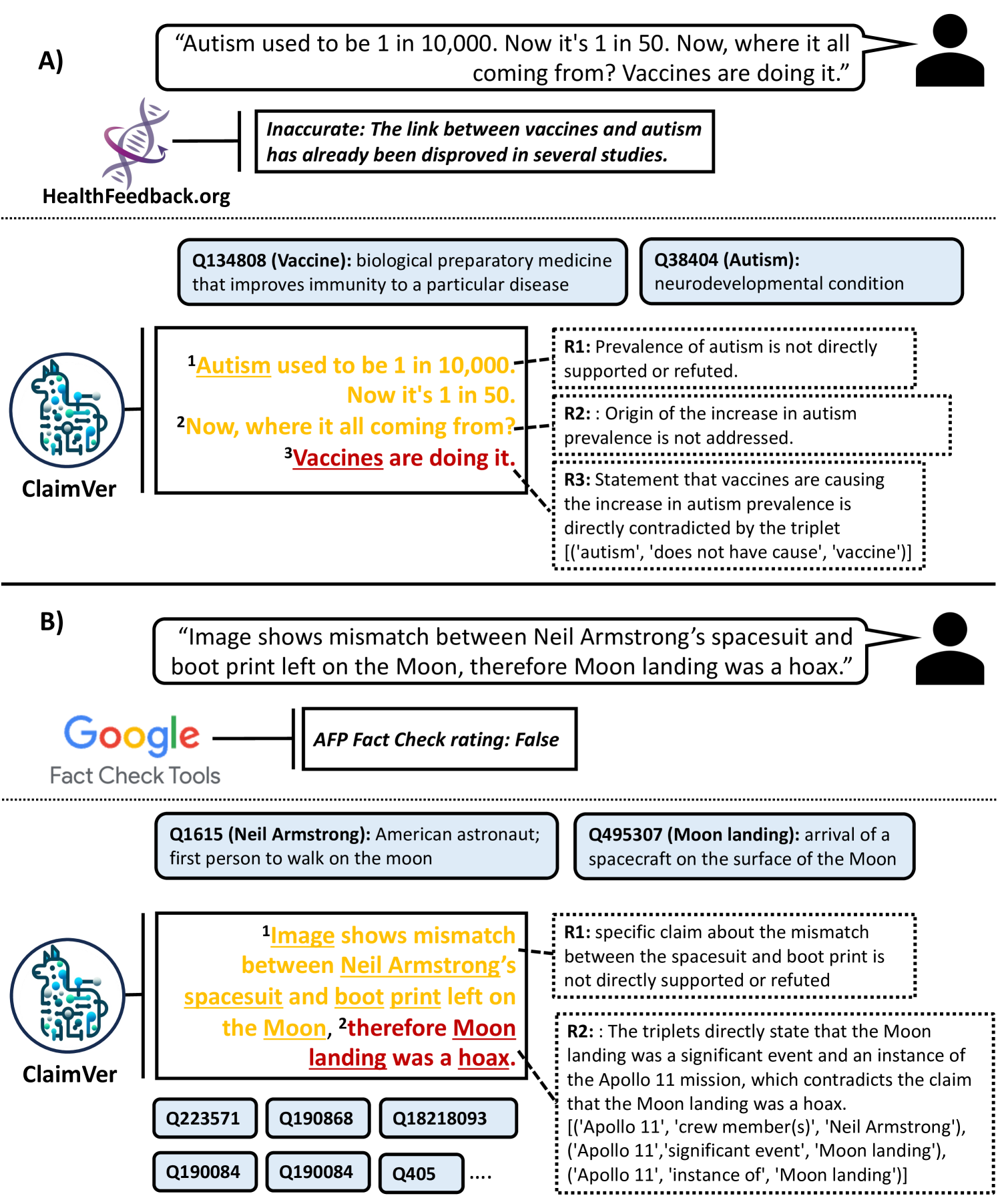</details> Figure 1: Demonstration of ClaimVer for claim verification and evidence attribution. (A) Text labeled as Inaccurate by HealthFeedback and ClaimVer’s predictions, rationale, and evidence. (B) Text labeled as False by Google Fact Check Tools and ClaimVer’s outputs. Predictions are color-coded (amber: extrapolatory, red: contradictory); $R_{i}$ : rationale; related wiki entities are displayed in boxes. ## 1 Introduction Misinformation and disinformation are longstanding issues, but the proliferation of AI tools that can generate information on demand has amplified these issues. Tools for fact-checking are not keeping pace with sophisticated text generation techniques. Even when they are effective, they lack appropriate explainability and granularity to be useful to users. Studies have shown that explanations are crucial for users to build trust in AI systems Rechkemmer and Yin (2022); Weitz et al. (2019); Shin (2021). Therefore, there is a need for a novel human-centric approach to text verification that offers usable and sufficiently granular explanations to inform and educate the user. Most fact-checkers, including widely used ones in deployment, issue blanket predictions that can lead to user misunderstandings. For instance, in Figure 1 (A), we observe that HealthFeedback https://healthfeedback.org/, a fact-checker for medical text, indicates that a misleading statement about the increase in Autism is inaccurate. However, there are multiple claims made in that text, which are not addressed by this tool. In fact, research does show that Autism cases have increased, but this is mostly attributed to increased testing Russell et al. (2015). Our method accurately breaks down the text into multiple claims and shows that the specific claim that vaccines are causing autism is indeed incorrect, attributing it to a fact from the Wikidata Vrandečić and Krötzsch (2014). It also provides a clear rationale as to why the first two claims cannot be determined, as there’s no conclusive evidence present in the KG. Such granular predictions, supported by justifications, significantly improve user confidence Rechkemmer and Yin (2022); Weitz et al. (2019); Shin (2021). Similarly, in Figure 1 (B), we notice that Google Fact Check Tools https://toolbox.google.com/factcheck/explorer provides a blanket label for an utterance denying the moon landing. In contrast, ClaimVer identifies the exact text span that can be conclusively proven incorrect and proceeds to provide specific information about the Apollo 11 mission and its crew members to refute the claim. All verified entities present in the text, along with their Wiki IDs and descriptions, are displayed for user reference. Prior research Rashkin et al. (2023); Yue et al. (2023); Thorne et al. (2019); Aly et al. (2021) typically validates text at the paragraph or sentence level without adequately enhancing user awareness by supplying key details such as rationale, match scores, or evidence. A KG-based approach allows for finer granularity, aiding in pinpointing specific inaccuracies like hallucinations in LLM-generated text or false claims in misleading text. Furthermore, if needed, broader-level metrics can be extracted from this detailed attribution. The assumption of one-to-one mapping between input and reference texts, prevalent in previous methods Rashkin et al. (2023); Yue et al. (2023); Thorne et al. (2019); Aly et al. (2021), does not hold if the given text consists of claims that can be mapped to more than one source. In contrast, utilizing a KG, which represents a consolidated body of knowledge, results in a more comprehensive evaluation. While most previous methods may not support scenarios with information spread across various references, querying a KG can yield triplets originally sourced from multiple documents. Additionally, procuring the specific spans of text required to evaluate claims from large text sources that may span several pages presents many challenges. In contrast, a KG captures only the most important relationships as nodes and links, providing a more efficient way to evaluate the claims. ## 2 Related Work Research on validating text has been ongoing for the past decade, while the concept of evidence attribution has gained increased attention in recent years, following the advent of generative models. Our method integrates fact verification and evidence attribution. In this section, we discuss recent advancements in both domains. ### 2.1 Fact Verification Fact verification is a task that is closely related to natural language inference (NLI) Conneau et al. (2017); Schick and Schütze (2020), in which given a premise, the task is to verify whether a hypothesis is an entailment, contradiction, or neutral. Similarly, in fact verification, the task is to check if a given text can be supported, refuted, or indeterminable, given a reference text. Recent studies in this domain show that LLMs can achieve high performance, and can be considerably reliable for verification tasks, even though they are prone to hallucations Guan et al. (2023). In Lee et al. (2020), the authors show that the inherent knowledge of LLMs could be used to perform fact verification. Other works Yao et al. (2022); Jiang et al. (2023b) have shown that using external knowledge is helpful for many reasoning-intensive tasks, and report enhanced performance on HotPotQA Yang et al. (2018) and FEVER Thorne et al. (2018). A wide variety of studies have established that LLMs are suitable for fact verification. For example, Dong and Smith (2021) enhanced accuracy of table-based fact verification by incorporating column-level cell rank information into pre-training. In FactScore, authors Min et al. (2023), introduce a new evaluation that breaks a long-form text generated by large language models (LMs) into individual atomic facts and calculates the proportion of these atomic facts that are substantiated by a credible knowledge base. ### 2.2 Evidence Attribution The distinction between evidence attribution and fact verification lies in the emphasis on identifying a source that can be attributed to the information. This task is becoming increasingly important, as generative models produce useful and impressive outputs, but without a frame of reference to validate them. In Rashkin et al. (2023), the authors present a framework named AIS (Attributable to Identified Sources) that specifies annotation guidelines and underlines the importance of attributing text to an external, verifiable, and independent source. Yue et al. (2023) demonstrate that LLMs can be utilized for automatic evaluation of attribution, operationalizing the guidelines presented in Rashkin et al. (2023). However, both of these works are primarily designed for the question-answering (QA) task. In contrast, our method is not restricted to QA and is designed to work with text in general. Furthermore, while these previous studies focus on sentence or paragraph levels, our approach extends to a more detailed and granular level of analysis. <details> <summary>x2.png Details</summary>  ### Visual Description \n ## Diagram: Knowledge Graph Based Claim Verification Pipeline ### Overview This diagram illustrates a pipeline for verifying claims using a knowledge graph. The pipeline takes input text, preprocesses it, retrieves relevant triplets from a knowledge graph, and then uses a finetuned language model to generate outputs including a claim, prediction, rationale, and a score. ### Components/Axes The diagram is segmented into four main sections: Input Text, Preprocessing, Knowledge Graph & Algorithm, and Outputs. Arrows indicate the flow of information. * **Input Text:** Contains the statement "Steven Tyler has never been a part of the band Aerosmith." * **Preprocessing:** Lists four steps: NER (Named Entity Recognition), Coreference, KG Entity Linking, and Compartmentalization. * **Knowledge Graph:** Depicted as a network of interconnected nodes (blue circles) representing entities and relationships. * **KG Triplet Retrieval Algorithm:** Represented by two interlocking gears. * **Finetuned ClaimVer LLM:** Represented by a brain-like structure. * **Outputs:** Contains four elements: Claim, Prediction, Relevant Triplets & TMS, and Rationale, and Score (KAS). ### Detailed Analysis or Content Details Let's break down each section: **1. Input Text:** The input text is: "Steven Tyler has never been a part of the band Aerosmith." **2. Preprocessing:** The preprocessing stage includes the following steps: * NER * Coreference * KG Entity Linking * Compartmentalization **3. Knowledge Graph & Algorithm:** The Knowledge Graph is a visual representation of interconnected entities. The KG Triplet Retrieval Algorithm retrieves relevant information from this graph. The output of this algorithm is fed into the Finetuned ClaimVer LLM. **4. Outputs:** * **Claim:** "Steven Tyler has never been a part of the band Aerosmith." (This is a restatement of the input text). * **Prediction:** "Contradictory" * **Relevant Triplets & TMS:** `[('Aerosmith', 'has part(s)', 'Steven Tyler')], 1.0` * **Rationale:** "This triplet establishes a clear relationship between Steven Tyler and Aerosmith, refuting the claim that he has never been associated with the band." * **Score (KAS):** 0.047 ### Key Observations * The pipeline identifies the input claim as "Contradictory" based on information retrieved from the Knowledge Graph. * The relevant triplet explicitly states that Steven Tyler *is* a part of Aerosmith, directly contradicting the input claim. * The KAS score is relatively low (0.047), suggesting a moderate level of confidence in the prediction. * The rationale clearly explains how the retrieved triplet supports the "Contradictory" prediction. ### Interpretation This diagram demonstrates a system for automated claim verification. The system leverages a knowledge graph to provide factual grounding for claims. The pipeline's ability to identify the contradiction between the input claim and the knowledge graph's data suggests a functional claim verification process. The low KAS score might indicate the need for further refinement of the LLM or the knowledge graph data. The system's strength lies in its ability to not only predict the veracity of a claim but also to provide a rationale based on evidence from the knowledge graph. The use of a Knowledge Graph and a Large Language Model (LLM) is a common approach to fact verification and reasoning tasks. The TMS (Truth Maintenance System) component, indicated in the "Relevant Triplets & TMS" section, suggests a mechanism for managing and evaluating the reliability of the retrieved information. 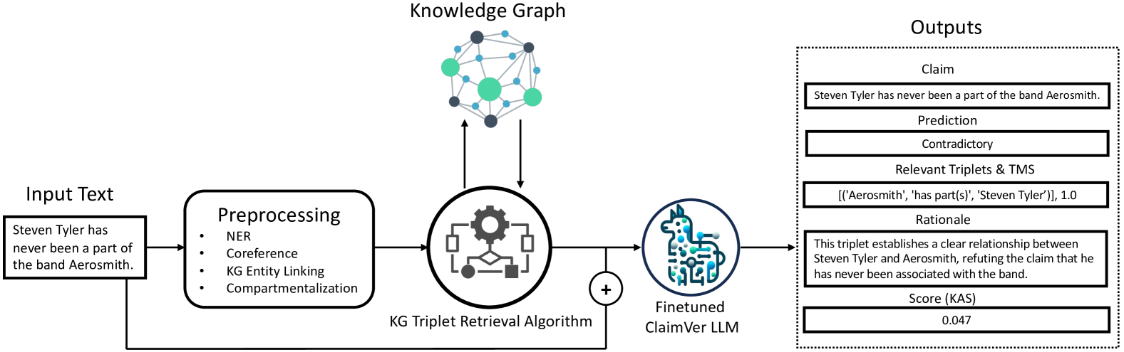</details> Figure 2: Flow of operations in the ClaimVer framework. Identified KG entity nodes during preprocessing inform the extraction of relevant triplets by the KG algorithm. Subsequently, these triplets and preprocessed text are then fed to a ClaimVer LLM, fine-tuned to operationalize the objective function. For each claim, the corresponding text span, prediction, relevant triplets, attribution scores, and rationale are generated. ## 3 Methodology In this section, we present the methodology for retrieving relevant triplets from the KG, fine-tuning LLM to process text at claim-level, verifying claims, tagging evidence for each prediction, and generating a rationale along with an attribution score that reflects the text’s validity. ### 3.1 Preprocessing Preprocessing involves multiple steps required to make the input text suitable for the subsequent operations. Since the nodes in a KG typically represent entities, performing Named Entity Recognition (NER) is necessary. In our work, we chose Wikidata Vrandečić and Krötzsch (2014) as the KG source; thus, we use an NER module suitable for Wiki entities Gerber (2023). However, the framework is sufficiently generic to support any kind of KG that models information in the form of triplets. As our analysis is performed at the claim level, coreference resolution Lee et al. (2017) becomes a necessary step to form localized claims that are semantically self-contained. If input text exceeds the context length, which depends on design choices, compartmentalization would be required. As a final step in preprocessing, we perform KG entity linking. This step tags all entities in the text that are present in the KG as nodes. ### 3.2 Relevant Triplets Retrieval Retrieving relevant triplets is a complex problem that has attracted attention from various research communities, and resulted in multiple approaches to address the challenge. While retrieving direct links between two given nodes in a KG is relatively straightforward, identifying complex paths that involve multiple hops is challenging. In our framework, we use Woolnet Gutiérrez and Patricio (2023), a multi-node Breadth-First Search (BFS) algorithm, to retrieve the most relevant triplets for a given claim present in the KG. This BFS algorithm initiates from multiple starting points and, at each step, searches for and processes all adjacent neighbors before advancing. It constructs a subgraph of visited nodes, tracking their origins, and distances from each BFS’s start. The algorithm expands each search tree one node at a time until paths intersect or reach a predefined maximum length. Upon intersection, it assesses if the discovered path meets the length criteria. If so, it logs the route, utilizing backtracking to trace the path to its origins, while ensuring there are no repetitions or cycles, thus maintaining a connection to a starting node. In our experiments, we allow for a maximum of three hops between any two given nodes, and a maximum of four potential paths. Adopting less stringent conditions leads to less relevant triplets. ### 3.3 Objective Function Previous works on evidence attribution tasks have established definitions for the categorization of input text with reference to a supporting source Rashkin et al. (2023); Gao et al. (2023); Bohnet et al. (2022); Yue et al. (2023). Similar to the formulation in Yue et al. (2023), we use three categories: Attributable, Extrapolatory, and Contradictory. However, there are two main differences that distinguish our approach from previous methods. First, we verify the input text against facts present in a KG, an aggregated information source constructed by integrating numerous data sources into a structure of triplets, instead of relying on a single reference. This approach eliminates the one-to-one dependency between the text and its information source. Second, we perform attribution with finer granularity, specifically at the claim level, involving a subtask of decomposing the input text into individual claims. We define our categories as follows: - Attributable: Triplets fully support the claim. - Extrapolatory: Triplets lack sufficient information to evaluate the claim. - Contradictory: Triplets contradict the claim. We formulate the objective function of our task as follows: where: - $input\_text$ : input text containing claim(s). - $ret\_triplets$ : retrieved triplets for the input text. - $claim\_span_{i}$ : $i^{th}$ claim extracted as a substring from $input\_text$ . - $claim\_pred_{i}$ : label predicted for $claim\_span_{i}$ . - $rel\_triplets_{i}$ : relevant subset of $ret\_triplets$ for $claim\_span_{i}$ . - $rationale_{i}$ : justification for $claim\_pred_{i}$ . - $n$ : total number of claims in $input\_text$ . This objective function encompasses two main sub-tasks: 1. Decomposing input text into claims. 1. Generating prediction and corresponding rationale for each claim by identifying relevant supporting triplets. ### 3.4 Fine-tuning LLMs The objective function shares similarities with the well-studied task of NLI Conneau et al. (2017); Schick and Schütze (2020). LLMs achieve state-of-the-art performance for NLI Chowdhery et al. (2023), making them a suitable choice to operationalize the objective function. Additionally, Yue et al. (2023) shows that LLMs can be used to automatically evaluate attribution to a given information source. However, these prior methods do not involve a complex sub-task, which is central to the proposed objective function, i.e., decomposing the input text into text spans that correspond to separate claims in the presence of multiple claims. It is crucial to perform both claim decomposition and attribution for all claims in a single step, as processing each claim individually can lead to an exponential increase in LLM queries, leading to significantly higher computational costs and latency issues. In order to perform attribution at the claim level, we need to fine-tune LLMs specifically for the proposed objective function (see § 3.3) using a custom dataset. This is necessary because, as of this writing, even the state-of-the-art model, OpenAI’s GPT-4 Achiam et al. (2023), does not perform satisfactorily right out of the box. Our custom dataset, built using two sequential complex prompts with GPT-4, enables us to fine-tune significantly smaller models. This approach distills the performance of a large proprietary model using a multi-query prompt pipeline into small open-source models with a compact zero-shot prompt. We make the weights of the fine-tuned models publicly available weights available on HuggingFace. We selected eight open-source LLMs with diverse sizes, ranging from 2B parameters to 10B parameters, to perform the fine-tuning: Gemma-2B-IT-Chat Team et al. (2024), Phi-3-mini-4k-Chat Javaheripi et al. (2023), Zephyr-7B-Beta-Chat Tunstall et al. (2023), Mistral-7B-v0.3-Chat Jiang et al. (2023a), Llama3-8B-Chat Touvron et al. (2023), and Solar-10.7B-Chat Kim et al. (2023). The models were fine-tuned using LoRA Hu et al. (2021) with 4-bit quantization and adapters with rank 8 Dettmers et al. (2024). The context length was set to 4096 tokens (for additional training details, refer § A.1) All models converged after 2 epochs, and high ROUGE-L Lin (2004) scores greater than 0.658 were achieved for each model. The instruction prompt used for fine-tuning is presented in Figure 3. Analyze text against provided triplets, classifying claims as "Attributable", "Contradictory", or "Extrapolatory". Justify your classification using the following structure: - "text_span": Text under evaluation. - "prediction": Category of the text (Attributable / Contradictory / Extrapolatory). - "triplets": Relevant triplets (if any, else "NA"). - "rationale": Reason for classification. For multiple claims, number each component (e.g., "text_span1", "prediction1",..). Use "NA" for inapplicable keys. Example: "text_span1": "Specific claim", "prediction1": "Attributable/Contradictory/Extrapolatory", "triplets1": "Relevant triplets", "rationale1": "Prediction justification", ... Input for analysis: -Text: {Input Text} -Triplets: {Retrieved Triplets} Figure 3: Instruction prompt for fine-tuned LLMs. ### 3.5 Computing Attribution Scores For various downstream tasks, such as ranking and filtering, a continuous score that reflects the validity of a given piece of text with respect to a KG is desirable. We propose the KG Attribution Score (KAS), which accomplishes this task with a high level of granularity, and is detailed in this section. #### 3.5.1 Claim Scores where, $y_{i}$ is $claim\_pred_{i}$ . For each claim, we assign a score that reflects the level of its validity, ranging from -1 (contradictory) to 2 (attributable). If a claim is predicted to be extrapolatory, yet has one or more relevant triplets, we assign that claim a score of 1, as there is still relevant information available even though it may not be sufficient to completely support or refute the claim. However, if there are no triplets at all, along with an extrapolatory prediction, we assign 0 as it does not add any useful information. While decomposing claims, the model might occasionally omit words, typically stop-words, and we assign 0 in those cases as well. #### 3.5.2 Triplets Match Score (TMS) This score reflects the extent of the match between the relevant triplets and the corresponding claim, and it can also serve as a proxy for the prediction confidence. Even though the prediction is made at the claim level, the triplets match score considers word-level matches in the computation. It can be computed as follows: where, $E(claim\_span_{i})$ and $E(rel\_triplet_{i})$ represent the sets of entities in $claim\_span_{i}$ and $rel\_triplet_{i}$ , respectively. $SS$ is the semantic similarity computed using the cosine similarity of text embeddings, and $EPR$ represents the ratio of entities in $E(claim\_span_{i})$ that are also present in $E(rel\_triplet_{i})$ . The parameters $\alpha$ and $\beta$ can be adjusted as needed; in our experiments, we use 0.5 for both. In cases where examples of an entity retrieved from the KG are used to support the prediction, instead of the entity itself, we may not have a direct overlap, and thus semantic similarity would be helpful. $EPR$ rewards the direct use of the entity, so a balance between both may be ideal in most cases. #### 3.5.3 KG Attribution Score (KAS) For the final KG Attribution Score (KAS), a continuous score between 0 and 1 is desirable, as this facilitates various downstream applications such as ranking, fine-tuning, and filtering. This can be achieved using a Sigmoid function. However, the standard Sigmoid function treats positive and negative scores equally. In most cases, higher penalties should be assigned for erroneous text than rewards for valid text. This requirement can be met using a modified Sigmoid function that penalizes mistakes by a factor of $\gamma$ : $$ \displaystyle\sigma_{\text{mod}}(x,\gamma)=\frac{1}{1+e^{-\gamma\cdot x}}, \displaystyle\text{where }\gamma=\begin{cases}\gamma=3&\text{if }x<0,\\ \gamma=1&\text{if }x\geq 0,\end{cases} \tag{4} $$ In our experiments, we set the value of $\gamma$ to 3. Finally, the modified Sigmoid function, applied to the summation of triplet match scores and claim scores, is used to generate KAS: $$ \displaystyle\text{KAS}=\sigma_{mod}(\sum_{i=1}^{n}[ \displaystyle TMS_{i}\cdot cs(y_{i})],\gamma) \tag{5} $$ ## 4 Dataset | Train Test | 3400 1000 | 5342 1677 | 998 316 | 3546 1068 | 798 293 | | --- | --- | --- | --- | --- | --- | Table 1: Distribution of fine-tuning dataset. Att: Attributable, Ext: Extrapolatory, Con: Contradictory. <details> <summary>x3.png Details</summary>  ### Visual Description ## Data Table: Triplet Extraction & Prediction Scores ### Overview The image presents a data table comparing "Input Text" with "Relevant Triplets", "Prediction (TMS)", "Rationale", and "KAS" (presumably a knowledge assessment score). The table appears to be evaluating the performance of a system in extracting key information (triplets) from text and providing a rationale for its predictions. ### Components/Axes The table has the following columns: 1. **Input Text:** The original text snippet. 2. **Relevant Triplets:** The key subject-predicate-object triplets extracted from the input text. 3. **Prediction (TMS):** A score (between 0 and 1) representing the system's confidence in its prediction. TMS likely stands for "Triplet Matching Score". 4. **Rationale:** An explanation of why the system made its prediction. The rationale is numbered (1, 2, 3). 5. **KAS:** A score (between 0 and 1) representing the knowledge assessment score. The table contains 6 rows, each representing a different input text. ### Detailed Analysis or Content Details Here's a reconstruction of the table's content, row by row: **Row 1:** * **Input Text:** "George O'Malley is a fictional character from the medical drama television series Grey's Anatomy, which airs on the American Broadcasting Company (ABC) in the United States." * **Relevant Triplets:** * (["Grey's Anatomy", "characters", "George O'Malley"] - 0.852) * (["Grey's Anatomy", "original broadcaster", "American Broadcasting Company"] - 0.637) * **Prediction (TMS):** 0.818 * **Rationale:** * "1: The triplet directly supports the claim that George O’Malley is a character in Grey’s Anatomy." * "2: The triplets confirm that Grey’s Anatomy airs on ABC, which is based in the United States, directly supporting the claim about the show’s broadcasting and location." * **KAS:** 0.818 **Row 2:** * **Input Text:** "Bane was portrayed as a tertiary villain by Robert Swenson in Batman & Robin, directed by Joel Schumacher, and Batman’s Back" * **Relevant Triplets:** * (["Batman & Robin", "cast member", "Robert Swenson"] - 0.788) * (["Batman & Robin", "director", "Joel Schumacher"] - 0.882) * **Prediction (TMS):** 0.752 * **Rationale:** * "1: The triplet directly supports the claim that Robert Swenson was involved in Batman & Robin, which is a requirement for the statement about his portrayal of Bane." * "2: The triplet directly supports the claim about the director of Batman & Robin, which is relevant to the context of the film." * **KAS:** 0.752 **Row 3:** * **Input Text:** "Crater Lake is the main feature of Crater Lake National Park and famous for its deep blue color and water clarity." * **Relevant Triplets:** * (["Crater Lake", "located in", "Crater Lake National Park"] - 0.942) * **Prediction (TMS):** 0.719 * **Rationale:** * "1: The triplet directly supports the claim that Crater Lake is a significant feature within Crater Lake National Park, as it is located within the protected area." * **KAS:** 0.719 **Row 4:** * **Input Text:** "Based in Blagnac, France, a suburb of Toulouse, and with significant activity across Europe, Airbus Operations S.A.S., is the corporate headquarters of Airbus, the European manufacturer of airplanes." * **Relevant Triplets:** * (["Airbus Operations S.A.S.", "country", "France"] - 0.505) * (["Airbus", "headquarters location", "Blagnac"] - 0.937) * **Prediction (TMS):** 0.583 * **Rationale:** * "1: Airbus confirms that Airbus Operations S.A.S. is in France." * "2: The triplet tells us that Airbus’ headquarters is in Toulouse about location of Airbus in France, supporting the statement about Airbus’ corporate headquarters and its proximity to Toulouse." * **KAS:** 0.583 **Row 5:** * **Input Text:** "The Jimi Hendrix Shrine is a memorial to Jimi Hendrix, located in Renton, Washington, and maintained by the Northwest Heritage Resources." * **Relevant Triplets:** * (["Jimi Hendrix Shrine", "dedicated to", "Jimi Hendrix"] - 0.912) * (["Jimi Hendrix Shrine", "located in", "Renton, Washington"] - 0.748) * **Prediction (TMS):** 0.742 * **Rationale:** * "1: The triplet directly supports the claim that the shrine is a memorial to Jimi Hendrix." * "2: The triplet confirms the location of the Jimi Hendrix Shrine, which is a requirement for the claim about its location in Renton, Washington." * **KAS:** 0.742 **Row 6:** * **Input Text:** "Francisco Franco’s Spanish Republican opponent, Indalecio Prieto, was born in Oviedo, Spain." * **Relevant Triplets:** * (["Indalecio Prieto", "birthplace", "Oviedo, Spain"] - 0.836) * **Prediction (TMS):** 0.683 * **Rationale:** * "1: The triplet directly supports the claim that Indalecio Prieto was born in Oviedo, Spain." * **KAS:** 0.683 ### Key Observations * The "Relevant Triplets" column consistently provides pairs of entities and their relationships. * The "Prediction (TMS)" scores are generally high, suggesting the system performs reasonably well. * The "Rationale" column provides a clear explanation of why the system identified those triplets as relevant. * The "KAS" scores are generally lower than the "TMS" scores, suggesting that while the system can identify relevant triplets, it may not fully understand the broader knowledge context. * There is a correlation between the number of triplets identified and the KAS score. Rows with more triplets tend to have higher KAS scores. ### Interpretation This data table demonstrates the performance of a natural language processing (NLP) system designed to extract structured information (triplets) from text. The system appears to be capable of identifying key entities and their relationships with a good degree of accuracy, as indicated by the TMS scores. However, the lower KAS scores suggest that the system's understanding of the underlying knowledge is less robust. The rationale provided for each prediction is valuable for understanding the system's reasoning process and identifying areas for improvement. The table highlights the challenges of moving beyond simple pattern matching to true semantic understanding in NLP. The system is better at identifying direct relationships (e.g., birthplace) than more complex or nuanced relationships. The data suggests that increasing the number of relevant triplets extracted from a text snippet can improve the overall knowledge assessment score. 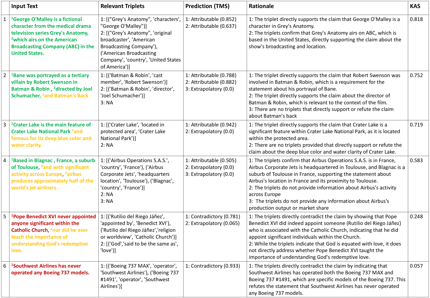</details> Table 2: Examples of claim-level attribution by the proposed method. The first column shows the numbered claims in the input text. Second column lists relevant triplets for each claim. Predictions and Triplets Match Score (TMS) are in the third column, while the rationale behind each prediction is in the fourth column. The Knowledge Graph Attribution Score (KAS) is shown in the last column. Model: Solar-10.7B-Chat. Open-domain Question Answering (QA) datasets, such as WikiQA Yang et al. (2015), HotPotQA Yang et al. (2018), PopQA Mallen et al. (2022), and EntityQuestions Sciavolino et al. (2021), as well as Fact Verification datasets like FEVER Thorne et al. (2019), FEVEROUS Aly et al. (2021), TabFacT Chen et al. (2019), and SEM-TAB-FACTS Wang et al. (2021a), provide texts along with corresponding reference contexts or attributable information sources. However, these datasets significantly differ from the type of data required to train and test our proposed objective function, primarily due to two major factors: (i) these datasets predominantly offer samples that are inherently attributable, and (ii) consist of atomic claims and/or one-to-one mappings between input and reference texts. To address the first limitation, prior work Yue et al. (2023) in attribution evaluation introduced new samples by modifying correct answers to generate contradictory instances. Yet, this adjustment alone is not sufficient for our use case because our method requires attribution at the claim level, and necessitates the automatic decomposition input text to claims. Consequently, as this task represents a novel challenge, we developed a new dataset that enables effective training and testing of the objective function. Considering the choice of our KG, which is Wikidata Vrandečić and Krötzsch (2014), we opted for WikiQA Yang et al. (2015) as it is closely associated with the Wiki ecosystem. Given that our method is designed for text validation in general, and is not limited to question answering, we retain only answers and discard the questions. Subsequently, we processed the answers following the steps detailed in Section 3.1, selecting entries containing two or more Wiki entities. This approach resulted in the exclusion of most single-word answers and other responses that are dependent on their corresponding questions and may lack comprehensibility without them. We utilize GPT-4 Achiam et al. (2023) to generate the initial version of the ground truth. Although GPT-4 can adhere to the instructions (refer to Figure 3) to a reasonable degree and responds in the required format with all necessary keys, it still underperforms in the overall task. The most frequent issue observed is the erroneous assignment of prediction labels. To remedy this issue, we designed a detailed prompt tailored for the given task, incorporating techniques such as few-shot, chain-of-thought Kojima et al. (2022), and other strategies OpenAI (2024); Nori et al. (2023) (full prompt in § A Figure 12). We also conducted manual checks to ensure only high-quality samples were retained, as research indicates that high alignment can be achieved with as few as 1,000 samples, provided they are of superior quality Zhou et al. (2023). The final dataset is comprised of two splits: the training split, based on the training split of WikiQA Yang et al. (2015), and a test split, derived from both the test and validation splits. The training split contains 3,400 samples, and since some entries feature multiple claims, there are a total of 5,342 claims within this split. Similarly, the test split includes 1,000 samples and 1,677 claims. The label counts for the claims are tabulated in Table 1. The dataset is publicly shared to facilitate further research in this direction dataset available on HuggingFace. ## 5 Experiments and Results In this section, we present the evaluation of our claim-level attribution method. The performance metrics of the fine-tuned LLMs, which operationalize the objective function, are presented in Tables 3 and 4. In Table 3, we observe that all models converge and achieve sufficiently high ROUGE-L and ROUGE-1 scores, with Mistral-7B-v0.3-Chat achieving the highest of 0.694 and 0.719 respectively. We also observe that the smaller model, Gemma-2B-IT-Chat with just 2B parameters, is also sufficiently compatible for this task as it attained a decent ROUGE-L score of 0.667. The first task of the proposed objective function (refer § 3.3), decomposing text into multiple claims, is somewhat subjective, and there could be multiple valid approaches due to linguistic complexities. For instance, example 4 in Table 2 has been decomposed into three claims, but the first could arguably be further decomposed to verify whether Blagnac is in France, and whether it is a suburb of Toulouse. Controlling the precise manner of decomposition is challenging, and might necessitate an additional step before the prediction step, involving separate processing for each claim. However, this option could prove to be impractical, as the number of LLM queries could increase exponentially. To accurately compute classification performance, we impose a strict strategy: the text span of the claim, the identified relevant triplets, and the prediction label must all exactly match the ground truth to be considered accurate. In Table 4, the second column indicates number of claims with text spans exactly matching the ground truth responses. Columns 3 to 6 present the accuracy, precision, recall, and F1 scores for these matching claims. The most performant model is Solar-10.7B-Chat, with 1031 exact matches out of 1677 claims in the test set. Additionally, the classification scores in all metrics are above 89%, which clearly demonstrates that the model can reliably differentiate between the classes attributable, extrapolatory, and contradictory. Table 2 showcases the claim-level attribution performed by our method. Each claim in the input text is numbered and color-coded to reflect its prediction: green for attributable, amber for extrapolatory, and red for contradictory. The examples are sorted in descending order by their KAS scores, which reflect the validity of the text. As expected, we observe more green at the top of the table and more amber and eventually red as we move down. Since the Wiki ecosystem is open-domain, we observe that the examples cover a wide range of topics, demonstrating that the method is adaptable to diverse inputs. In the first example in 2, the input text is decomposed into two claims, both of which are attributable. The first claim is supported by a single triplet in the KG, while the second claim can be supported by combining two triplets. The second example presents more challenges for evaluation due to its complex sentence structure, but ClaimVer accurately identifies that the third claim regarding Batman’s Back is neither supported nor refuted by the triplets, as indicated in the rationale. In the third example, we note that the first claim is predicted to be attributable with a high triplet match score of 0.942 since there is a triplet that clearly supports the location description of Crater Lake. However, as there is no information regarding the water characteristics, the second claim is categorized as extrapolatory. In the fourth example, the first claim alone requires three triplets combined as supporting evidence, illustrating the method’s ability to handle complex multi-hop paths within the KG. The second and third claims are predicted to be extrapolatory, since there are no triplets concerning Airbus’s market share, or its activities in Europe, as highlighted in the model’s rationale. It is noteworthy that the context provided in the third claim is crucial for the first claim to be comprehensible, demonstrating why individual claim evaluation may be suboptimal. Interestingly, in the fifth example, the method identifies a specific instance from the KG to refute a general claim, citing the appointment of Rutilio del Riego Jáñez. Similarly, in the sixth example, the method provides specific instances, quoting two distinct Boeing 737 models to demonstrate contradiction with a high triplet match score. | Gemma-2B-IT-Chat Phi-3-mini-4k-Chat Zephyr-7B-Beta-Chat | 2B 4B 7B | 0.667 0.658 0.686 | 0.692 0.685 0.712 | | --- | --- | --- | --- | | Vicuna-7B-v1.5-Chat | 7B | 0.676 | 0.700 | | Mistral-7B-v0.3-Chat | 7B | 0.694 | 0.719 | | Gemma-7B-IT-Chat | 7B | 0.678 | 0.703 | | Llama3-8B-Chat | 8B | 0.679 | 0.705 | | Solar-10.7B-Chat | 10B | 0.689 | 0.714 | Table 3: ROUGE scores on the test set ( $n=1,000$ ). | Gemma-2B-IT-Chat Phi-3-mini-4k-Chat Zephyr-7B-Beta-Chat | 895 882 978 | 77.09 72.22 85.89 | 77.20 78.10 87.41 | 77.09 72.22 85.89 | 74.24 72.86 86.16 | | --- | --- | --- | --- | --- | --- | | Vicuna-7B-v1.5-Chat | 898 | 79.62 | 78.83 | 79.62 | 78.84 | | Mistral-7B-v0.3-Chat | 1002 | 86.63 | 87.03 | 86.63 | 86.73 | | Gemma-7B-IT-Chat | 940 | 82.87 | 84.09 | 82.87 | 83.17 | | Llama3-8B-Chat | 959 | 80.92 | 85.48 | 80.92 | 81.36 | | Solar-10.7B-Chat | 1031 | 89.23 | 89.52 | 89.23 | 89.30 | Table 4: Scores on matching claims in the test set ( $n=1677$ ). #MC: number of matching claims. ## 6 Discussion The susceptibility of LLMs to generating factually incorrect statements is an alarming concern as LLM-powered services become increasingly popular for seeking advice and information. The democratization of generative models has also had adverse effects, such as increasing misinformation Monteith et al. (2024). To arm end-users with the tools necessary to combat being misinformed, it is crucial to develop text-validation methods that are human-centric, and prioritize user engagement, understanding, and informativeness. We design our method with these principles in mind: we make predictions at the claim level, and identify text spans within the given text, that can be color-coded and presented to the user. The proposed method also generates easily comprehensible explanations along with the prediction and evidence, thus reducing the cognitive burden on the end-user, and making the process user-friendly. The usability and evaluation of these systems should align with human needs and capabilities. Chatbots, such as ChatGPT Achiam et al. (2023), serve a wide array of tasks; therefore, the text validation method should be adaptable to various domains. While KGs like Wikidata Vrandečić and Krötzsch (2014) are considered open-domain, the implementation of more specialized KGs, along with corresponding routing algorithms may be necessary to support a broader range of topics. For instance, a common-sense KG Hwang et al. (2020) would be more useful in validating non-factoid answers that involve logic. Furthermore, the maintenance efficiency of our approach aligns well with the need for sustainable, long-term AI solutions. In a world where information is constantly evolving, the ability to update and maintain AI systems with minimal effort is not just a convenience, but a necessity. This directly ties into the ethical implications of AI, where outdated or incorrect information can lead to harmful decisions. By leveraging existing, well-maintained KGs, we can ensure that AI systems remain accurate and relevant over time. ## 7 Conclusion In this paper, we present ClaimVer, a framework for text verification and evidence attribution at the claim level by leveraging information present in KGs. In contrast to other methods, ClaimVer eliminates the one-to-one mapping between input and reference text, allowing for layered interpretation and handling of distributed information. In addition to these primary functions, ClaimVer incorporates human-centric design principles by offering clear, concise explanations for each claim prediction—an important characteristic for building user trust and enhancing usability. Furthermore, we introduce an attribution score, which enhances its applicability across a wide range of downstream tasks. Finally, we share ClaimVer fine-tuned LLMs to facilitate further exploration of this research direction. ## 8 Limitations Limitations of LLMs for Fact Verification. Like most ML models, LLMs are prone to erroneous predictions, which is particularly concerning in sensitive applications such as handling misinformation. Despite this, they remain the most performant techniques for fact verification and related tasks like NLI Yue et al. (2023); Wang et al. (2021b). Therefore, while it is reasonable to use the best option available, fact verification systems relying on LLMs should be utilized with caution and necessary validations. Limitations of Knowledge Graphs. While there are several advantages associated with using KGs, we also acknowledge the presence of known issues, such as knowledge coverage and the efforts required to keep these sources up-to-date. For our solution, we assume that the KG is up-to-date and possesses adequate coverage. However, this may not always be the case, and thus the most suitable technique should be adopted after considering the specific requirements of a particular use case. Another point to consider is that the proposed method does not provide traditional citations to articles, although it may be possible to retrieve that information from the KG, if information source mapping has been properly maintained. Variations in Claim Decomposition. Decomposing text into multiple claims is a complex linguistic task that often results in multiple valid decompositions. Although this may not impact usability if the prediction, rationale, and text spans are comprehensible and supported by facts from the KG, it poses a challenge for evaluating model performance. One potential approach is to operate at the token level instead of the span level, but this would significantly complicate the problem space. Additionally, token-level verification and attribution would require substantially higher compute resources, necessitating further studies to assess their value and impact on system usability and reliability. LLM Reasoning Errors. Previous works have demonstrated that using LLM reasoning for tasks like fact verification, evidence attribution, and NLI can yield impressive results, surpassing alternative approaches Yue et al. (2023); Wang et al. (2021b). However, LLM reasoning can still be flawed. In our work, we impose validations to minimize LLM mistakes by performing membership checks for supporting triplets and string matching for text spans. Yet, validating reasoning remains an open problem with ongoing research efforts. Fine-tuning Dataset Limitations. To build the fine-tuning dataset, we utilized GPT-4 with two detailed sequential prompts designed in accordance with OpenAI’s recommendations OpenAI (2024) and previous works Nori et al. (2023). Despite employing techniques like few-shot prompting with state-of-the-art LLMs, we still observe mistakes, indicating the complexity of this problem. To address this, we conducted manual checks to minimize errors and share the dataset with the research community for further improvement. ## 9 Ethical Concerns Our work presents a scalable and interpretable framework for fact-checking textual claims. To promote the exploration of this important problem space, we fine-tune and share open-source LLMs that are well-aligned to the framework’s objective function. While the models we provide perform better than the publicly available base models for our specific task, they still share similar weaknesses such as erroneous reasoning. To address this as best as we can, we have incorporated and described ways to mitigate these issues to the extent possible. We believe the benefits of this work outweigh any potential risks. ## References - Achiam et al. (2023) Josh Achiam, Steven Adler, Sandhini Agarwal, Lama Ahmad, Ilge Akkaya, Florencia Leoni Aleman, Diogo Almeida, Janko Altenschmidt, Sam Altman, Shyamal Anadkat, et al. 2023. Gpt-4 technical report. arXiv preprint arXiv:2303.08774. - Aly et al. (2021) Rami Aly, Zhijiang Guo, Michael Schlichtkrull, James Thorne, Andreas Vlachos, Christos Christodoulopoulos, Oana Cocarascu, and Arpit Mittal. 2021. Feverous: Fact extraction and verification over unstructured and structured information. arXiv preprint arXiv:2106.05707. - Bohnet et al. (2022) Bernd Bohnet, Vinh Q Tran, Pat Verga, Roee Aharoni, Daniel Andor, Livio Baldini Soares, Massimiliano Ciaramita, Jacob Eisenstein, Kuzman Ganchev, Jonathan Herzig, et al. 2022. Attributed question answering: Evaluation and modeling for attributed large language models. arXiv preprint arXiv:2212.08037. - Chen et al. (2019) Wenhu Chen, Hongmin Wang, Jianshu Chen, Yunkai Zhang, Hong Wang, Shiyang Li, Xiyou Zhou, and William Yang Wang. 2019. Tabfact: A large-scale dataset for table-based fact verification. arXiv preprint arXiv:1909.02164. - Chowdhery et al. (2023) Aakanksha Chowdhery, Sharan Narang, Jacob Devlin, Maarten Bosma, Gaurav Mishra, Adam Roberts, Paul Barham, Hyung Won Chung, Charles Sutton, Sebastian Gehrmann, et al. 2023. Palm: Scaling language modeling with pathways. Journal of Machine Learning Research, 24(240):1–113. - Conneau et al. (2017) Alexis Conneau, Douwe Kiela, Holger Schwenk, Loic Barrault, and Antoine Bordes. 2017. Supervised learning of universal sentence representations from natural language inference data. arXiv preprint arXiv:1705.02364. - Dettmers et al. (2024) Tim Dettmers, Artidoro Pagnoni, Ari Holtzman, and Luke Zettlemoyer. 2024. Qlora: Efficient finetuning of quantized llms. Advances in Neural Information Processing Systems, 36. - Dong and Smith (2021) Rui Dong and David A Smith. 2021. Structural encoding and pre-training matter: Adapting bert for table-based fact verification. In Proceedings of the 16th Conference of the European Chapter of the Association for Computational Linguistics: Main Volume, pages 2366–2375. - Gao et al. (2023) Luyu Gao, Zhuyun Dai, Panupong Pasupat, Anthony Chen, Arun Tejasvi Chaganty, Yicheng Fan, Vincent Zhao, Ni Lao, Hongrae Lee, Da-Cheng Juan, et al. 2023. Rarr: Researching and revising what language models say, using language models. In Proceedings of the 61st Annual Meeting of the Association for Computational Linguistics (Volume 1: Long Papers), pages 16477–16508. - Gerber (2023) Emanuel Gerber. 2023. spacy module for linking text to wikidata items. https://github.com/egerber/spaCy-entity-linker. Accessed: 2024-02-26. - Guan et al. (2023) Jian Guan, Jesse Dodge, David Wadden, Minlie Huang, and Hao Peng. 2023. Language models hallucinate, but may excel at fact verification. arXiv preprint arXiv:2310.14564. - Gutiérrez and Patricio (2023) Torres Gutiérrez and Cristóbal Patricio. 2023. Sistema visual para explorar subgrafos temáticos en wikidata. - Hu et al. (2021) Edward J Hu, Yelong Shen, Phillip Wallis, Zeyuan Allen-Zhu, Yuanzhi Li, Shean Wang, Lu Wang, and Weizhu Chen. 2021. Lora: Low-rank adaptation of large language models. arXiv preprint arXiv:2106.09685. - Hwang et al. (2020) Jena D. Hwang, Chandra Bhagavatula, Ronan Le Bras, Jeff Da, Keisuke Sakaguchi, Antoine Bosselut, and Yejin Choi. 2020. Comet-atomic 2020: On symbolic and neural commonsense knowledge graphs. In AAAI Conference on Artificial Intelligence. - Javaheripi et al. (2023) Mojan Javaheripi, Sébastien Bubeck, Marah Abdin, Jyoti Aneja, Sebastien Bubeck, Caio César Teodoro Mendes, Weizhu Chen, Allie Del Giorno, Ronen Eldan, Sivakanth Gopi, et al. 2023. Phi-2: The surprising power of small language models. Microsoft Research Blog. - Jiang et al. (2023a) Albert Q Jiang, Alexandre Sablayrolles, Arthur Mensch, Chris Bamford, Devendra Singh Chaplot, Diego de las Casas, Florian Bressand, Gianna Lengyel, Guillaume Lample, Lucile Saulnier, et al. 2023a. Mistral 7b. arXiv preprint arXiv:2310.06825. - Jiang et al. (2023b) Zhengbao Jiang, Frank F Xu, Luyu Gao, Zhiqing Sun, Qian Liu, Jane Dwivedi-Yu, Yiming Yang, Jamie Callan, and Graham Neubig. 2023b. Active retrieval augmented generation. arXiv preprint arXiv:2305.06983. - Kim et al. (2023) Dahyun Kim, Chanjun Park, Sanghoon Kim, Wonsung Lee, Wonho Song, Yunsu Kim, Hyeonwoo Kim, Yungi Kim, Hyeonju Lee, Jihoo Kim, et al. 2023. Solar 10.7 b: Scaling large language models with simple yet effective depth up-scaling. arXiv preprint arXiv:2312.15166. - Kojima et al. (2022) Takeshi Kojima, Shixiang Shane Gu, Machel Reid, Yutaka Matsuo, and Yusuke Iwasawa. 2022. Large language models are zero-shot reasoners. Advances in neural information processing systems, 35:22199–22213. - Lee et al. (2017) Kenton Lee, Luheng He, Mike Lewis, and Luke Zettlemoyer. 2017. End-to-end neural coreference resolution. arXiv preprint arXiv:1707.07045. - Lee et al. (2020) Nayeon Lee, Belinda Z Li, Sinong Wang, Wen-tau Yih, Hao Ma, and Madian Khabsa. 2020. Language models as fact checkers? arXiv preprint arXiv:2006.04102. - Lin (2004) Chin-Yew Lin. 2004. ROUGE: A package for automatic evaluation of summaries. In Text Summarization Branches Out, pages 74–81, Barcelona, Spain. Association for Computational Linguistics. - Mallen et al. (2022) Alex Mallen, Akari Asai, Victor Zhong, Rajarshi Das, Hannaneh Hajishirzi, and Daniel Khashabi. 2022. When not to trust language models: Investigating effectiveness and limitations of parametric and non-parametric memories. arXiv preprint arXiv:2212.10511. - Min et al. (2023) Sewon Min, Kalpesh Krishna, Xinxi Lyu, Mike Lewis, Wen tau Yih, Pang Wei Koh, Mohit Iyyer, Luke Zettlemoyer, and Hannaneh Hajishirzi. 2023. Factscore: Fine-grained atomic evaluation of factual precision in long form text generation. Preprint, arXiv:2305.14251. - Monteith et al. (2024) Scott Monteith, Tasha Glenn, John R Geddes, Peter C Whybrow, Eric Achtyes, and Michael Bauer. 2024. Artificial intelligence and increasing misinformation. The British Journal of Psychiatry, 224(2):33–35. - Nori et al. (2023) Harsha Nori, Yin Tat Lee, Sheng Zhang, Dean Carignan, Richard Edgar, Nicolo Fusi, Nicholas King, Jonathan Larson, Yuanzhi Li, Weishung Liu, et al. 2023. Can generalist foundation models outcompete special-purpose tuning? case study in medicine. arXiv preprint arXiv:2311.16452. - OpenAI (2024) OpenAI. 2024. Best practices for prompt engineering with the openai api. https://help.openai.com/en/articles/6654000-best-practices-for-prompt-engineering-with-the-openai-api. Accessed:2024-01-11. - Rashkin et al. (2023) Hannah Rashkin, Vitaly Nikolaev, Matthew Lamm, Lora Aroyo, Michael Collins, Dipanjan Das, Slav Petrov, Gaurav Singh Tomar, Iulia Turc, and David Reitter. 2023. Measuring attribution in natural language generation models. Computational Linguistics, pages 1–64. - Rechkemmer and Yin (2022) Amy Rechkemmer and Ming Yin. 2022. When confidence meets accuracy: Exploring the effects of multiple performance indicators on trust in machine learning models. In Proceedings of the 2022 chi conference on human factors in computing systems, pages 1–14. - Russell et al. (2015) Ginny Russell, Stephan Collishaw, Jean Golding, Susan E Kelly, and Tamsin Ford. 2015. Changes in diagnosis rates and behavioural traits of autism spectrum disorder over time. BJPsych open, 1(2):110–115. - Schick and Schütze (2020) Timo Schick and Hinrich Schütze. 2020. Exploiting cloze questions for few shot text classification and natural language inference. arXiv preprint arXiv:2001.07676. - Sciavolino et al. (2021) Christopher Sciavolino, Zexuan Zhong, Jinhyuk Lee, and Danqi Chen. 2021. Simple entity-centric questions challenge dense retrievers. In Proceedings of the 2021 Conference on Empirical Methods in Natural Language Processing, pages 6138–6148, Online and Punta Cana, Dominican Republic. Association for Computational Linguistics. - Shin (2021) Donghee Shin. 2021. The effects of explainability and causability on perception, trust, and acceptance: Implications for explainable ai. International Journal of Human-Computer Studies, 146:102551. - Team et al. (2024) Gemma Team, Thomas Mesnard, Cassidy Hardin, Robert Dadashi, Surya Bhupatiraju, Shreya Pathak, Laurent Sifre, Morgane Rivière, Mihir Sanjay Kale, Juliette Love, et al. 2024. Gemma: Open models based on gemini research and technology. arXiv preprint arXiv:2403.08295. - Thorne et al. (2018) James Thorne, Andreas Vlachos, Christos Christodoulopoulos, and Arpit Mittal. 2018. Fever: a large-scale dataset for fact extraction and verification. arXiv preprint arXiv:1803.05355. - Thorne et al. (2019) James Thorne, Andreas Vlachos, Oana Cocarascu, Christos Christodoulopoulos, and Arpit Mittal. 2019. The FEVER2.0 shared task. In Proceedings of the Second Workshop on Fact Extraction and VERification (FEVER), pages 1–6, Hong Kong, China. Association for Computational Linguistics. - Touvron et al. (2023) Hugo Touvron, Louis Martin, Kevin Stone, Peter Albert, Amjad Almahairi, Yasmine Babaei, Nikolay Bashlykov, Soumya Batra, Prajjwal Bhargava, Shruti Bhosale, et al. 2023. Llama 2: Open foundation and fine-tuned chat models. arXiv preprint arXiv:2307.09288. - Tunstall et al. (2023) Lewis Tunstall, Edward Beeching, Nathan Lambert, Nazneen Rajani, Kashif Rasul, Younes Belkada, Shengyi Huang, Leandro von Werra, Clémentine Fourrier, Nathan Habib, et al. 2023. Zephyr: Direct distillation of lm alignment. arXiv preprint arXiv:2310.16944. - Vrandečić and Krötzsch (2014) Denny Vrandečić and Markus Krötzsch. 2014. Wikidata: a free collaborative knowledgebase. Communications of the ACM, 57(10):78–85. - Wang et al. (2021a) Nancy XR Wang, Diwakar Mahajan, Marina Danilevsky, and Sara Rosenthal. 2021a. Semeval-2021 task 9: Fact verification and evidence finding for tabular data in scientific documents (sem-tab-facts). arXiv preprint arXiv:2105.13995. - Wang et al. (2021b) Sinong Wang, Han Fang, Madian Khabsa, Hanzi Mao, and Hao Ma. 2021b. Entailment as few-shot learner. arXiv preprint arXiv:2104.14690. - Weitz et al. (2019) Katharina Weitz, Dominik Schiller, Ruben Schlagowski, Tobias Huber, and Elisabeth André. 2019. " do you trust me?" increasing user-trust by integrating virtual agents in explainable ai interaction design. In Proceedings of the 19th ACM International Conference on Intelligent Virtual Agents, pages 7–9. - Yang et al. (2015) Yi Yang, Wen-tau Yih, and Christopher Meek. 2015. WikiQA: A challenge dataset for open-domain question answering. In Proceedings of the 2015 Conference on Empirical Methods in Natural Language Processing, pages 2013–2018, Lisbon, Portugal. Association for Computational Linguistics. - Yang et al. (2018) Zhilin Yang, Peng Qi, Saizheng Zhang, Yoshua Bengio, William W Cohen, Ruslan Salakhutdinov, and Christopher D Manning. 2018. Hotpotqa: A dataset for diverse, explainable multi-hop question answering. arXiv preprint arXiv:1809.09600. - Yao et al. (2022) Shunyu Yao, Jeffrey Zhao, Dian Yu, Nan Du, Izhak Shafran, Karthik Narasimhan, and Yuan Cao. 2022. React: Synergizing reasoning and acting in language models. arXiv preprint arXiv:2210.03629. - Yue et al. (2023) Xiang Yue, Boshi Wang, Kai Zhang, Ziru Chen, Yu Su, and Huan Sun. 2023. Automatic evaluation of attribution by large language models. arXiv preprint arXiv:2305.06311. - Zhou et al. (2023) Chunting Zhou, Pengfei Liu, Puxin Xu, Srini Iyer, Jiao Sun, Yuning Mao, Xuezhe Ma, Avia Efrat, Ping Yu, Lili Yu, et al. 2023. Lima: Less is more for alignment. arXiv preprint arXiv:2305.11206. 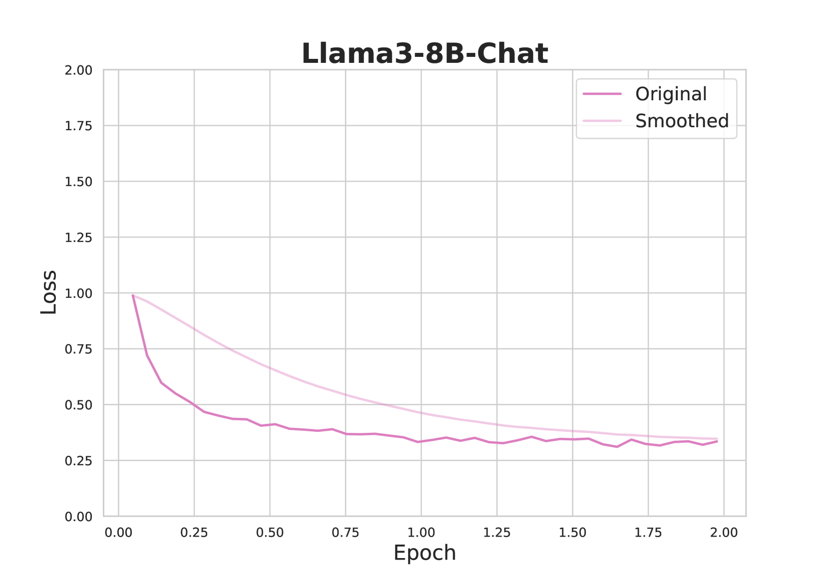## Appendix A Appendix ### A.1 Training Details In this section, we present the training parameters used for fine-tuning each model, along with their corresponding loss plots. All models converged after two epochs, achieving ROUGE-L Lin (2004) scores greater than 0.658, with the best model reaching 0.719. <details> <summary>x4.png Details</summary>  ### Visual Description ## Line Chart: Llama3-8B-Chat Loss vs. Epoch ### Overview This chart displays the loss function of a Llama3-8B-Chat model over epochs. Two lines are plotted: the original loss and a smoothed version of the loss. The chart aims to visualize the model's training progress and stability. ### Components/Axes * **Title:** Llama3-8B-Chat (positioned top-center) * **X-axis:** Epoch (ranging from approximately 0.00 to 2.00, with tick marks at 0.25 intervals) * **Y-axis:** Loss (ranging from approximately 0.00 to 2.00, with tick marks at 0.25 intervals) * **Legend:** Located in the top-right corner. * "Original" - represented by a purple line. * "Smoothed" - represented by a pink line. ### Detailed Analysis The chart shows two lines representing loss over epochs. **Original Loss (Purple Line):** The line starts at approximately 0.95 at Epoch 0.00. It exhibits a steep downward trend until approximately Epoch 0.50, reaching a minimum loss of around 0.40. From Epoch 0.50 to Epoch 2.00, the line fluctuates between approximately 0.25 and 0.40, showing some oscillation but generally remaining relatively stable. Specific data points (approximate): * Epoch 0.00: Loss = 0.95 * Epoch 0.25: Loss = 0.70 * Epoch 0.50: Loss = 0.40 * Epoch 0.75: Loss = 0.35 * Epoch 1.00: Loss = 0.30 * Epoch 1.25: Loss = 0.32 * Epoch 1.50: Loss = 0.28 * Epoch 1.75: Loss = 0.35 * Epoch 2.00: Loss = 0.30 **Smoothed Loss (Pink Line):** The smoothed line also starts at approximately 0.95 at Epoch 0.00. It shows a similar downward trend to the original line, but it is less steep and more consistent. The smoothed line reaches a minimum loss of around 0.25 at approximately Epoch 1.00. From Epoch 1.00 to Epoch 2.00, the smoothed line remains relatively stable, fluctuating between approximately 0.25 and 0.30. Specific data points (approximate): * Epoch 0.00: Loss = 0.95 * Epoch 0.25: Loss = 0.65 * Epoch 0.50: Loss = 0.45 * Epoch 0.75: Loss = 0.35 * Epoch 1.00: Loss = 0.25 * Epoch 1.25: Loss = 0.28 * Epoch 1.50: Loss = 0.27 * Epoch 1.75: Loss = 0.29 * Epoch 2.00: Loss = 0.30 ### Key Observations * Both the original and smoothed loss curves demonstrate a decreasing trend, indicating that the model is learning and improving over epochs. * The smoothed line is less noisy than the original line, suggesting that it provides a more stable representation of the model's learning progress. * The loss appears to converge after approximately Epoch 0.50, with both lines fluctuating around a relatively low loss value. * The difference between the original and smoothed lines is minimal, indicating that the smoothing process does not significantly alter the overall trend. ### Interpretation The chart suggests that the Llama3-8B-Chat model is successfully training, as evidenced by the decreasing loss function. The smoothing of the loss curve helps to visualize the underlying trend and reduce the impact of noise. The convergence of the loss after a certain number of epochs indicates that the model has reached a stable state and further training may not yield significant improvements. The relatively small difference between the original and smoothed loss curves suggests that the model's learning process is consistent and predictable. The data suggests that the model is learning effectively and efficiently, and that the training process is stable and well-behaved. The model appears to have converged to a good solution, as indicated by the low and stable loss values. </details> Figure 4: Fine-tuning loss plots for Llama3-8B-Chat. | Parameter Base Model ROUGE-L | Value meta-llama/Meta-Llama-3-8B-Instruct 0.679 | | --- | --- | | ROUGE-1 | 0.705 | | Fine-Tuning Type | LoRA | | LoRA Alpha | 16 | | LoRA Rank | 8 | | Cutoff Length | 4096 | | Gradient Accumulation Steps | 8 | | Learning Rate | 5.0e-05 | | LR Scheduler Type | Cosine | | Number of Training Epochs | 2.0 | | Optimizer | AdamW | | Quantization Bit | 4 | Table 5: Fine-tuning Parameters for Llama3-8B-Chat <details> <summary>x5.png Details</summary>  ### Visual Description \n ## Line Chart: Mistral-7B-v0.3-Chat Loss vs. Epoch ### Overview This image presents a line chart illustrating the relationship between 'Loss' and 'Epoch' for a model named "Mistral-7B-v0.3-Chat". Two lines are plotted: one representing the 'Original' loss and the other representing the 'Smoothed' loss. The chart appears to track the model's training progress, showing how the loss function changes over epochs. ### Components/Axes * **Title:** Mistral-7B-v0.3-Chat * **X-axis:** Epoch (ranging from approximately 0.00 to 2.00) * **Y-axis:** Loss (ranging from approximately 0.00 to 2.00) * **Legend:** * Original (Purple line) * Smoothed (Gray line) * **Gridlines:** A light gray grid is present, aiding in reading values. ### Detailed Analysis The chart displays two lines representing loss over epochs. **Original Line (Purple):** The line starts at approximately 0.65 loss at Epoch 0.00. It exhibits a steep downward slope initially, decreasing to around 0.35 loss by Epoch 0.25. The slope then becomes less steep, leveling off around 0.25 loss between Epochs 0.50 and 2.00. There are minor fluctuations around this level. Approximate data points: * Epoch 0.00: Loss ≈ 0.65 * Epoch 0.25: Loss ≈ 0.35 * Epoch 0.50: Loss ≈ 0.28 * Epoch 1.00: Loss ≈ 0.25 * Epoch 1.50: Loss ≈ 0.24 * Epoch 2.00: Loss ≈ 0.26 **Smoothed Line (Gray):** The smoothed line begins at approximately 0.75 loss at Epoch 0.00. It also shows a downward trend, but is less volatile than the original line. It reaches a minimum of around 0.22 loss at Epoch 1.00. After Epoch 1.00, the smoothed line fluctuates slightly around 0.23-0.25 loss. Approximate data points: * Epoch 0.00: Loss ≈ 0.75 * Epoch 0.25: Loss ≈ 0.50 * Epoch 0.50: Loss ≈ 0.35 * Epoch 1.00: Loss ≈ 0.22 * Epoch 1.50: Loss ≈ 0.24 * Epoch 2.00: Loss ≈ 0.25 ### Key Observations * Both the original and smoothed loss curves demonstrate a decreasing trend, indicating that the model is learning and improving over epochs. * The smoothed line is less noisy than the original line, suggesting that it represents a more stable and generalized view of the loss function. * The original loss appears to fluctuate more, potentially indicating overfitting or sensitivity to specific training batches. * The loss values appear to converge towards a stable level around 0.25, suggesting that the model is approaching a point of diminishing returns in terms of further training. ### Interpretation The chart illustrates the training process of the Mistral-7B-v0.3-Chat model. The decreasing loss values indicate successful learning. The difference between the original and smoothed loss curves suggests that the model's performance is somewhat variable during training, but the smoothing process provides a more robust representation of the overall trend. The convergence of the loss curves around 0.25 suggests that the model has reached a point where further training may not yield significant improvements. This could be a good indication to stop training and evaluate the model's performance on a validation dataset. The smoothing likely represents a moving average, reducing the impact of individual epoch variations and highlighting the overall learning trajectory. The fact that the smoothed line consistently remains above the original line suggests that the smoothing process is not masking any significant improvements, but rather providing a clearer view of the underlying trend. 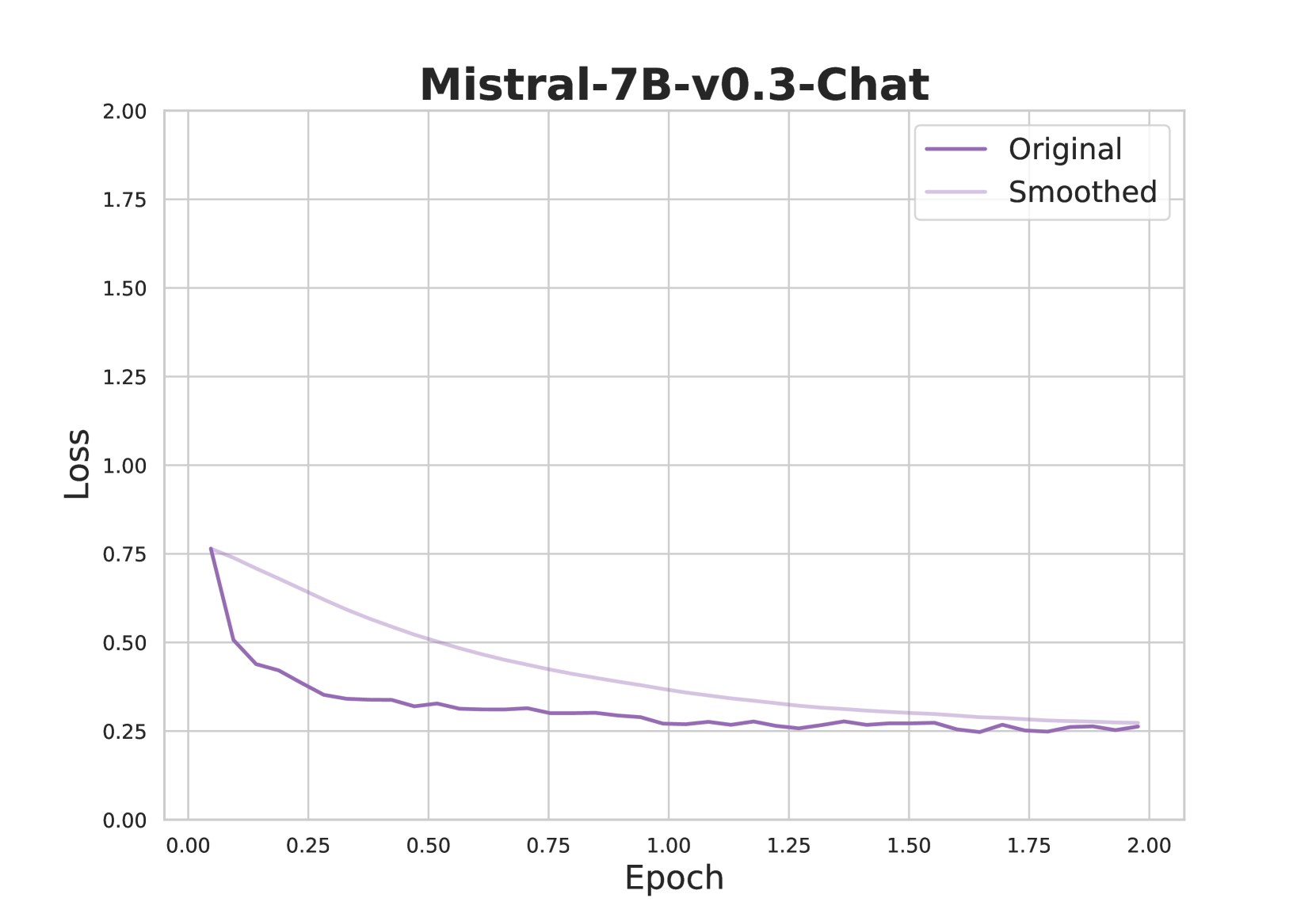</details> Figure 5: Fine-tuning loss plots for Mistral-7B-v0.3-Chat. | Parameter Base Model ROUGE-L | Value mistralai/Mistral-7B-Instruct-v0.3 0.694 | | --- | --- | | ROUGE-1 | 0.719 | | Fine-Tuning Type | LoRA | | LoRA Alpha | 16 | | LoRA Rank | 8 | | Cutoff Length | 4096 | | Gradient Accumulation Steps | 8 | | Learning Rate | 5.0e-05 | | LR Scheduler Type | Cosine | | Number of Training Epochs | 2.0 | | Optimizer | AdamW | | Quantization Bit | 4 | Table 6: Fine-tuning Parameters for Mistral-7B-v0.3-Chat <details> <summary>x6.png Details</summary>  ### Visual Description ## Line Chart: Phi-3-mini-4k-Chat Training Loss ### Overview This image presents a line chart illustrating the training loss of a model named "Phi-3-mini-4k-Chat" over epochs. Two lines are plotted: "Original" loss and "Smoothed" loss. The chart aims to visualize how the model's loss decreases during training, with the smoothed line representing a trendline. ### Components/Axes * **Title:** Phi-3-mini-4k-Chat (positioned at the top-center) * **X-axis:** Epoch (ranging from approximately 0.00 to 2.00, with tick marks at 0.25 intervals) * **Y-axis:** Loss (ranging from approximately 0.00 to 2.00, with tick marks at 0.25 intervals) * **Legend:** Located in the top-right corner. * "Original" - represented by an orange line. * "Smoothed" - represented by a light-grey line. ### Detailed Analysis **Original Loss (Orange Line):** The "Original" loss line starts at approximately 0.75 at Epoch 0.00. It exhibits a steep downward trend until approximately Epoch 0.25, reaching a loss of around 0.40. From Epoch 0.25 to Epoch 1.00, the line continues to decrease, but at a slower rate, reaching a loss of approximately 0.25. Between Epoch 1.00 and Epoch 2.00, the line fluctuates around 0.25, with minor oscillations. Specific data points (approximate): * Epoch 0.00: Loss = 0.75 * Epoch 0.25: Loss = 0.40 * Epoch 0.50: Loss = 0.32 * Epoch 0.75: Loss = 0.28 * Epoch 1.00: Loss = 0.25 * Epoch 1.25: Loss = 0.26 * Epoch 1.50: Loss = 0.24 * Epoch 1.75: Loss = 0.27 * Epoch 2.00: Loss = 0.26 **Smoothed Loss (Light-Grey Line):** The "Smoothed" loss line begins at approximately 0.75 at Epoch 0.00. It shows a consistent downward trend, though less erratic than the "Original" line. The smoothed line reaches a loss of approximately 0.25 by Epoch 1.00 and remains relatively stable around that value until Epoch 2.00. Specific data points (approximate): * Epoch 0.00: Loss = 0.75 * Epoch 0.25: Loss = 0.55 * Epoch 0.50: Loss = 0.40 * Epoch 0.75: Loss = 0.32 * Epoch 1.00: Loss = 0.25 * Epoch 1.25: Loss = 0.24 * Epoch 1.50: Loss = 0.24 * Epoch 1.75: Loss = 0.25 * Epoch 2.00: Loss = 0.25 ### Key Observations * Both the "Original" and "Smoothed" loss curves demonstrate a decreasing trend, indicating that the model is learning and improving over epochs. * The "Smoothed" line provides a clearer visualization of the overall loss trend, filtering out some of the noise present in the "Original" loss curve. * The "Original" loss exhibits more fluctuations, suggesting that the training process is not perfectly smooth and may be sensitive to individual batches of data. * The loss appears to converge around a value of 0.25 after approximately 1.0 epoch. ### Interpretation The chart suggests that the "Phi-3-mini-4k-Chat" model is successfully being trained, as evidenced by the decreasing loss values. The smoothing of the loss curve indicates that the model's performance is stabilizing over time. The convergence of the loss around 0.25 suggests that the model has reached a point of diminishing returns, where further training may not significantly improve its performance. The fluctuations in the "Original" loss curve could be due to the stochastic nature of the training process, or potentially indicate the need for adjustments to the learning rate or other hyperparameters. The difference between the original and smoothed loss shows the variance in the training process. The smoothed loss is a good indicator of the overall trend, while the original loss shows the actual performance at each epoch. 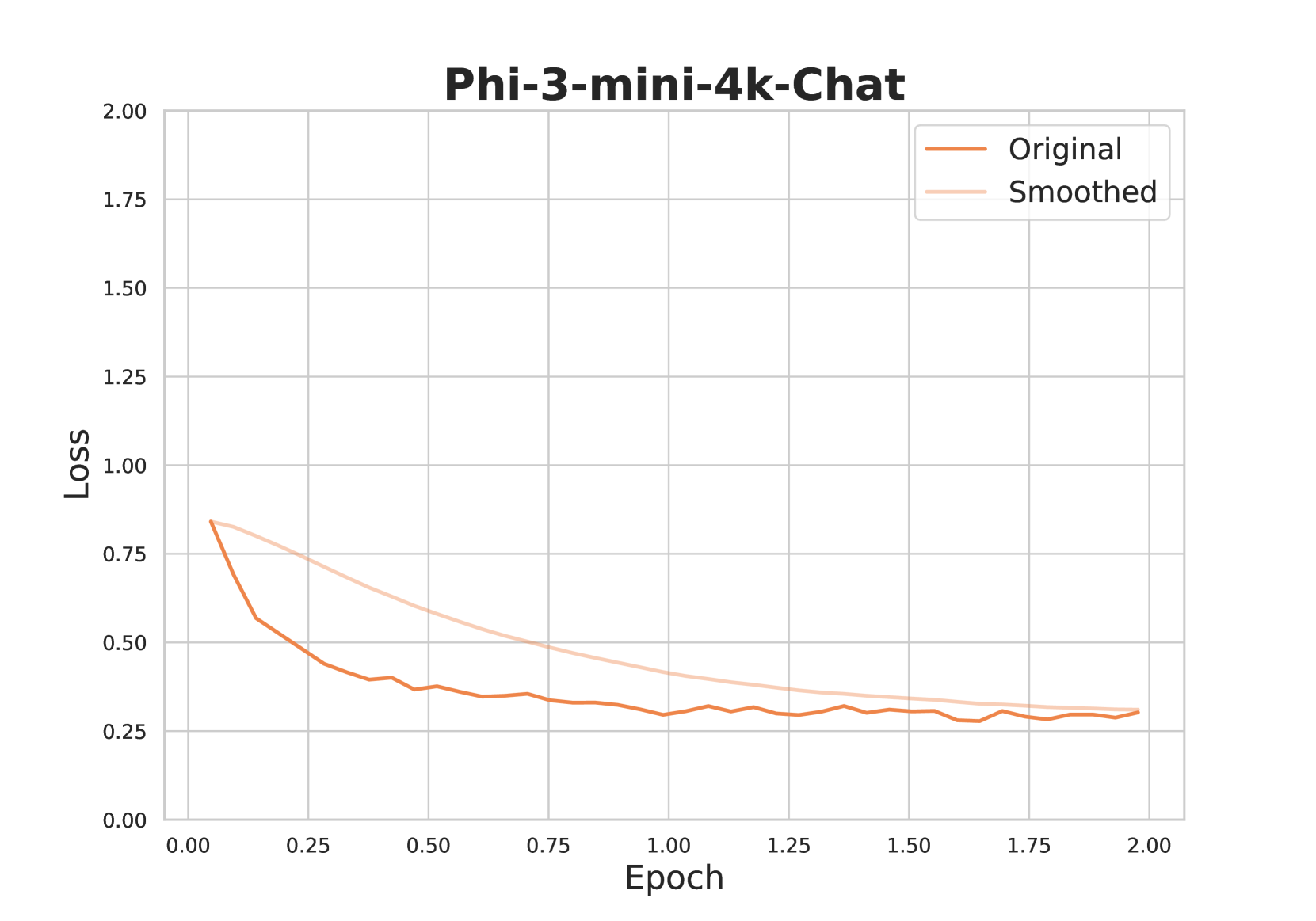</details> Figure 6: Fine-tuning loss plots for Phi-3-mini-4k-Chat. | Parameter Base Model ROUGE-L | Value microsoft/Phi-3-mini-4k-instruct 0.658 | | --- | --- | | ROUGE-1 | 0.685 | | Fine-Tuning Type | LoRA | | LoRA Alpha | 16 | | LoRA Rank | 8 | | Cutoff Length | 4096 | | Gradient Accumulation Steps | 8 | | Learning Rate | 5.0e-05 | | LR Scheduler Type | Cosine | | Number of Training Epochs | 2.0 | | Optimizer | AdamW | | Quantization Bit | 4 | Table 7: Fine-tuning Parameters for Phi-3-mini-4k-Chat <details> <summary>x7.png Details</summary>  ### Visual Description ## Line Chart: Solar-10.7B-Chat Loss vs. Epoch ### Overview This image presents a line chart illustrating the relationship between 'Loss' and 'Epoch' for a model named "Solar-10.7B-Chat". Two data series are plotted: 'Original' and 'Smoothed', representing different processing methods applied to the loss data. The chart aims to visualize how the loss function changes over training epochs. ### Components/Axes * **Title:** Solar-10.7B-Chat * **X-axis:** Epoch (ranging from approximately 0.00 to 2.00) * **Y-axis:** Loss (ranging from approximately 0.00 to 2.00) * **Legend:** * Original (Black line) * Smoothed (Gray line) * **Gridlines:** A light gray grid is present, aiding in reading values. ### Detailed Analysis The chart displays two lines representing the loss function over epochs. **Original Line (Black):** The 'Original' line starts at approximately 0.75 loss at Epoch 0.00. It exhibits a steep downward slope initially, decreasing to around 0.30 loss by Epoch 0.25. The slope then gradually decreases, leveling off around 0.25 loss between Epochs 0.75 and 2.00. 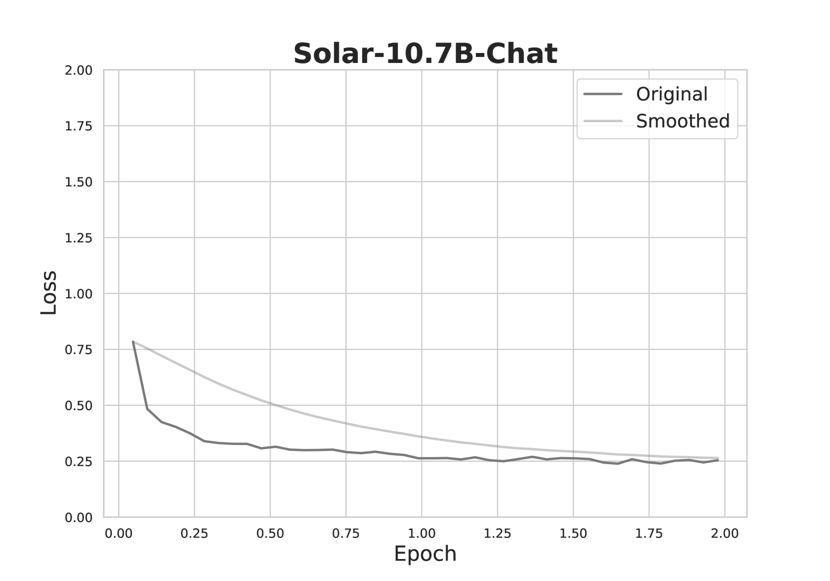Approximate data points: * Epoch 0.00: Loss ≈ 0.75 * Epoch 0.25: Loss ≈ 0.30 * Epoch 0.50: Loss ≈ 0.27 * Epoch 0.75: Loss ≈ 0.26 * Epoch 1.00: Loss ≈ 0.25 * Epoch 1.25: Loss ≈ 0.25 * Epoch 1.50: Loss ≈ 0.25 * Epoch 1.75: Loss ≈ 0.25 * Epoch 2.00: Loss ≈ 0.25 **Smoothed Line (Gray):** The 'Smoothed' line begins at approximately 0.65 loss at Epoch 0.00. It also shows a decreasing trend, but it is less steep than the 'Original' line. The smoothed line reaches around 0.20 loss by Epoch 0.25 and continues to decrease, stabilizing around 0.20 loss between Epochs 1.00 and 2.00. Approximate data points: * Epoch 0.00: Loss ≈ 0.65 * Epoch 0.25: Loss ≈ 0.20 * Epoch 0.50: Loss ≈ 0.20 * Epoch 0.75: Loss ≈ 0.21 * Epoch 1.00: Loss ≈ 0.20 * Epoch 1.25: Loss ≈ 0.20 * Epoch 1.50: Loss ≈ 0.20 * Epoch 1.75: Loss ≈ 0.20 * Epoch 2.00: Loss ≈ 0.20 ### Key Observations * Both the 'Original' and 'Smoothed' loss curves demonstrate a decreasing trend, indicating that the model is learning and improving over epochs. * The 'Smoothed' line consistently shows lower loss values than the 'Original' line, suggesting that the smoothing process reduces the variance in the loss function. * The rate of loss reduction decreases over time for both lines, indicating diminishing returns from further training. * The 'Original' line appears to fluctuate more than the 'Smoothed' line, which is expected given the smoothing process. ### Interpretation The chart illustrates the training process of the Solar-10.7B-Chat model. The loss function, representing the error between the model's predictions and the actual values, decreases as the model is trained for more epochs. The 'Smoothed' line suggests that applying a smoothing technique to the loss data can provide a more stable and less noisy representation of the training progress. The convergence of both lines towards a stable loss value indicates that the model is approaching a point of diminishing returns, and further training may not significantly improve performance. The difference between the two lines could be due to the smoothing algorithm used, which likely averages out short-term fluctuations in the loss function. This type of visualization is crucial for monitoring model training, identifying potential issues (e.g., overfitting), and determining when to stop training. </details> Figure 7: Fine-tuning loss plots for SOLAR-10.7B-Chat. | Parameter Base Model ROUGE-L | Value upstage/SOLAR-10.7B-Instruct-v1.0 0.689 | | --- | --- | | ROUGE-1 | 0.714 | | Fine-Tuning Type | LoRA | | LoRA Alpha | 16 | | LoRA Rank | 8 | | Cutoff Length | 4096 | | Gradient Accumulation Steps | 8 | | Learning Rate | 5.0e-05 | | LR Scheduler Type | Cosine | | Number of Training Epochs | 2.0 | | Optimizer | AdamW | | Quantization Bit | 4 | Table 8: Fine-tuning Parameters for SOLAR-10.7B-Chat <details> <summary>x8.png Details</summary>  ### 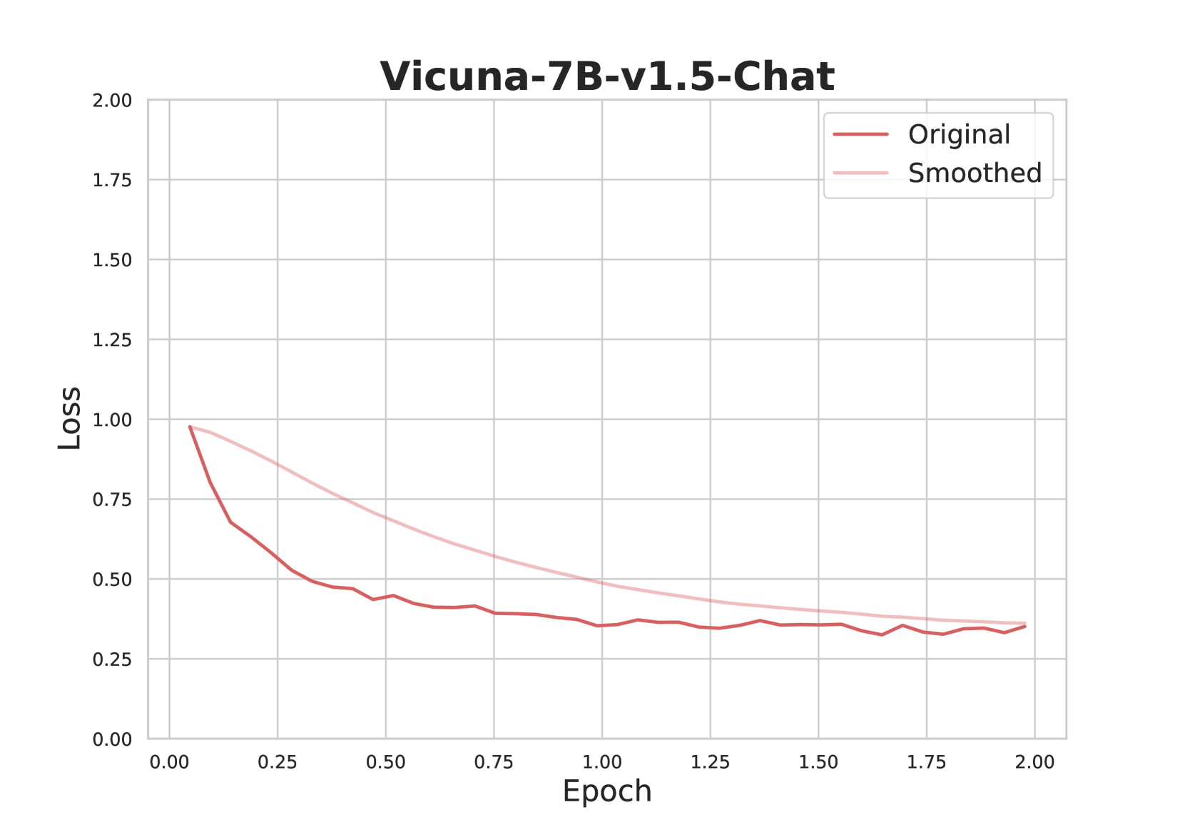Visual Description \n ## Line Chart: Vicuna-7B-v1.5-Chat Loss vs. Epoch ### Overview This chart displays the loss function of a model (Vicuna-7B-v1.5-Chat) over epochs during training. Two lines are plotted: the original loss and a smoothed version of the loss. The chart aims to visualize the training process and how the loss changes with each epoch. ### Components/Axes * **Title:** Vicuna-7B-v1.5-Chat * **X-axis:** Epoch (ranging from approximately 0.00 to 2.00) * **Y-axis:** Loss (ranging from approximately 0.00 to 2.00) * **Legend:** * Original (represented by a dark red line) * Smoothed (represented by a light red line) * **Grid:** A light gray grid is present to aid in reading values. ### Detailed Analysis The chart shows two lines representing the loss over epochs. **Original Loss (Dark Red Line):** The line starts at approximately 0.98 at Epoch 0.00. It then exhibits a steep downward trend until approximately Epoch 0.25, reaching a value of around 0.40. From Epoch 0.25 to Epoch 0.75, the line continues to decrease, but at a slower rate, reaching a minimum of approximately 0.35 at Epoch 0.65. After Epoch 0.75, the line fluctuates between approximately 0.30 and 0.45, showing some oscillation but generally remaining relatively stable. At Epoch 2.00, the value is approximately 0.32. **Smoothed Loss (Light Red Line):** The smoothed line starts at approximately 0.98 at Epoch 0.00, mirroring the original line. It also shows a downward trend, but it is less steep and more consistent than the original line. The smoothed line reaches a value of approximately 0.50 at Epoch 0.25. It continues to decrease, reaching a minimum of approximately 0.38 at Epoch 0.75. From Epoch 0.75 to Epoch 2.00, the smoothed line remains relatively stable, fluctuating between approximately 0.35 and 0.40. At Epoch 2.00, the value is approximately 0.37. ### Key Observations * Both the original and smoothed loss curves demonstrate a decreasing trend, indicating that the model is learning and improving over epochs. * The smoothed line is less noisy and provides a clearer representation of the overall trend. * The original loss curve exhibits more fluctuations, suggesting that the training process is not perfectly smooth. * The loss appears to converge after approximately 1.0 epoch, as the lines become relatively stable. * The difference between the original and smoothed loss is minimal after Epoch 1.0. ### Interpretation The chart suggests that the Vicuna-7B-v1.5-Chat model is successfully being trained, as the loss function is decreasing over time. The smoothing of the loss curve helps to visualize the underlying trend and reduce the impact of noise. The convergence of the loss after approximately 1.0 epoch indicates that the model is approaching a stable state. The fluctuations in the original loss curve could be due to various factors, such as the stochastic nature of the training process or the complexity of the dataset. The relatively small difference between the original and smoothed loss curves suggests that the smoothing process is not significantly altering the overall trend. This data is useful for monitoring the training process, identifying potential issues (e.g., overfitting or underfitting), and determining when to stop training. </details> Figure 8: Fine-tuning loss plots for Vicuna-7B-v1.5-Chat. | Parameter Base Model ROUGE-L | Value lmsys/vicuna-7b-v1.5 0.676 | | --- | --- | | ROUGE-1 | 0.700 | | Fine-Tuning Type | LoRA | | LoRA Alpha | 16 | | LoRA Rank | 8 | | Cutoff Length | 4096 | | Gradient Accumulation Steps | 8 | | Learning Rate | 5.0e-05 | | LR Scheduler Type | Cosine | | Number of Training Epochs | 2.0 | | Optimizer | AdamW | | Quantization Bit | 4 | Table 9: Fine-tuning Parameters for Vicuna-7B-v1.5-Chat <details> <summary>x9.png Details</summary>  ### 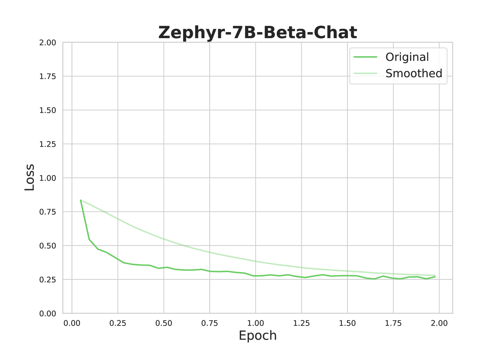Visual Description \n ## Line Chart: Zephyr-7B-Beta-Chat Loss vs. Epoch ### Overview This line chart depicts the loss function of a model named "Zephyr-7B-Beta-Chat" over epochs. Two lines are plotted: one representing the original loss and the other representing a smoothed version of the loss. The chart aims to visualize the model's training progress and stability. ### Components/Axes * **Title:** Zephyr-7B-Beta-Chat (centered at the top) * **X-axis:** Epoch (ranging from approximately 0.00 to 2.00) * **Y-axis:** Loss (ranging from approximately 0.00 to 2.00) * **Legend:** Located in the top-right corner. * "Original" (represented by a green line) * "Smoothed" (represented by a light green line) * **Gridlines:** Present to aid in reading values. ### Detailed Analysis The chart shows two lines representing loss over epochs. **Original Loss (Green Line):** The line starts at approximately 0.80 at Epoch 0.00. It exhibits a steep downward slope until approximately Epoch 0.25, reaching a value of around 0.30. From Epoch 0.25 to Epoch 1.00, the slope becomes less steep, gradually decreasing to approximately 0.25. Between Epoch 1.00 and Epoch 2.00, the line fluctuates around 0.25, with minor oscillations. Approximate data points: * Epoch 0.00: Loss = 0.80 * Epoch 0.25: Loss = 0.30 * Epoch 0.50: Loss = 0.27 * Epoch 1.00: Loss = 0.25 * Epoch 1.50: Loss = 0.24 * Epoch 2.00: Loss = 0.25 **Smoothed Loss (Light Green Line):** The smoothed line starts at approximately 0.75 at Epoch 0.00. It also shows a downward trend, but it is less pronounced than the original line. The smoothed line reaches a value of around 0.25 by Epoch 0.50 and continues to decrease slowly, reaching approximately 0.22 by Epoch 2.00. Approximate data points: * Epoch 0.00: Loss = 0.75 * Epoch 0.25: Loss = 0.45 * Epoch 0.50: Loss = 0.25 * Epoch 1.00: Loss = 0.23 * Epoch 1.50: Loss = 0.22 * Epoch 2.00: Loss = 0.22 ### Key Observations * Both the original and smoothed loss curves demonstrate a decreasing trend, indicating that the model is learning and improving over epochs. * The smoothed line is consistently above the original line, suggesting that the smoothing process introduces a slight bias towards higher loss values. * The original loss curve exhibits more fluctuations than the smoothed curve, indicating that the smoothing process reduces noise and provides a more stable representation of the loss. * The rate of loss reduction decreases as the number of epochs increases, suggesting that the model is approaching convergence. ### Interpretation The chart illustrates the training process of the Zephyr-7B-Beta-Chat model. The decreasing loss values indicate that the model is successfully learning to minimize the error between its predictions and the actual values. The smoothed loss curve provides a clearer view of the overall trend, while the original loss curve reveals the inherent noise and fluctuations in the training process. The convergence of both curves towards a stable loss value suggests that the model has reached a point where further training may not yield significant improvements. The difference between the two lines suggests that the smoothing process is effective in reducing noise, but it also introduces a slight bias. This chart is a standard visualization for monitoring the training of machine learning models, and it provides valuable insights into the model's performance and stability. </details> Figure 9: Fine-tuning loss plots for Zephyr-7B-Beta-Chat. | Parameter Base Model ROUGE-L | Value HuggingFaceH4/zephyr-7b-beta 0.686 | | --- | --- | | ROUGE-1 | 0.712 | | Fine-Tuning Type | LoRA | | LoRA Alpha | 16 | | LoRA Rank | 8 | | Cutoff Length | 4096 | | Gradient Accumulation Steps | 8 | | Learning Rate | 5.0e-05 | | LR Scheduler Type | Cosine | | Number of Training Epochs | 2.0 | | Optimizer | AdamW | | Quantization Bit | 4 | Table 10: Fine-tuning Parameters for Zephyr-7B-Beta-Chat <details> <summary>x10.png Details</summary>  ### 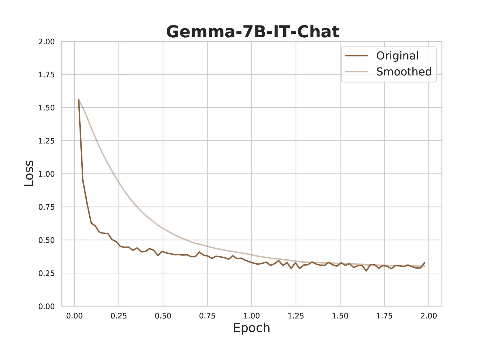Visual Description ## Line Chart: Gemma-7B-IT-Chat Training Loss ### Overview This image presents a line chart illustrating the training loss of the Gemma-7B-IT-Chat model over epochs. Two lines are plotted: "Original" loss and "Smoothed" loss, both representing the loss function's value as training progresses. The chart spans approximately 2 epochs, with loss values ranging from 0.0 to 2.0. ### Components/Axes * **Title:** Gemma-7B-IT-Chat (positioned at the top-center) * **X-axis:** Epoch (ranging from 0.0 to 2.0, with tick marks at 0.25 intervals) * **Y-axis:** Loss (ranging from 0.0 to 2.0, with tick marks at 0.25 intervals) * **Legend:** Located in the top-right corner, containing two entries: * "Original" - represented by a dark brown line. * "Smoothed" - represented by a light brown line. ### Detailed Analysis The chart displays two lines representing the loss function over epochs. **Original Loss (Dark Brown Line):** The line starts at approximately 1.6 at Epoch 0.0. It exhibits a steep downward trend until approximately Epoch 0.25, reaching a value of around 0.6. From Epoch 0.25 to Epoch 1.0, the line continues to decrease, but at a slower rate, reaching a value of approximately 0.35. Between Epoch 1.0 and Epoch 2.0, the line fluctuates around 0.25-0.35, showing minor oscillations. **Smoothed Loss (Light Brown Line):** The smoothed line begins at approximately 1.6 at Epoch 0.0, mirroring the original line. It also shows a rapid decrease until Epoch 0.25, reaching a value of around 0.6. From Epoch 0.25 to Epoch 1.0, the smoothed line continues to decrease, reaching a value of approximately 0.3. From Epoch 1.0 to Epoch 2.0, the smoothed line remains relatively stable, fluctuating around 0.25-0.3. **Specific Data Points (Approximate):** | Epoch | Original Loss | Smoothed Loss | |-------|--------------|--------------| | 0.00 | 1.6 | 1.6 | | 0.25 | 0.6 | 0.6 | | 0.50 | 0.45 | 0.4 | | 0.75 | 0.38 | 0.35 | | 1.00 | 0.35 | 0.3 | | 1.25 | 0.32 | 0.28 | | 1.50 | 0.30 | 0.27 | | 1.75 | 0.28 | 0.26 | | 2.00 | 0.25 | 0.25 | ### Key Observations * Both the original and smoothed loss curves demonstrate a clear decreasing trend, indicating that the model is learning and improving over epochs. * The smoothed line is less noisy than the original line, providing a clearer visualization of the overall trend. * The rate of loss reduction slows down after Epoch 0.25, suggesting diminishing returns from further training. * The loss appears to converge around a value of 0.25-0.35 after Epoch 1.0. ### Interpretation The chart illustrates the training process of the Gemma-7B-IT-Chat model. The decreasing loss values indicate that the model is successfully minimizing the error between its predictions and the actual values. The smoothing of the loss curve helps to identify the underlying trend, filtering out short-term fluctuations. The convergence of the loss after a certain number of epochs suggests that the model has reached a point of diminishing returns, and further training may not significantly improve its performance. The relatively low final loss value (around 0.25-0.35) indicates that the model has learned a good representation of the training data. This data suggests the model is learning effectively, but further analysis (e.g., validation loss) would be needed to assess generalization performance and prevent overfitting. </details> Figure 10: Fine-tuning loss plots for Gemma-7B-IT-Chat. | Parameter Base Model ROUGE-L | Value google/gemma-7b-it 0.678 | | --- | --- | | ROUGE-1 | 0.703 | | Fine-Tuning Type | LoRA | | LoRA Alpha | 16 | | LoRA Rank | 8 | | Cutoff Length | 4096 | | Gradient Accumulation Steps | 8 | | Learning Rate | 5.0e-05 | | LR Scheduler Type | Cosine | | Number of Training Epochs | 2.0 | | Optimizer | AdamW | | Quantization Bit | 4 | Table 11: Fine-tuning Parameters for Gemma-7B-IT-Chat <details> <summary>x11.png Details</summary>  ### 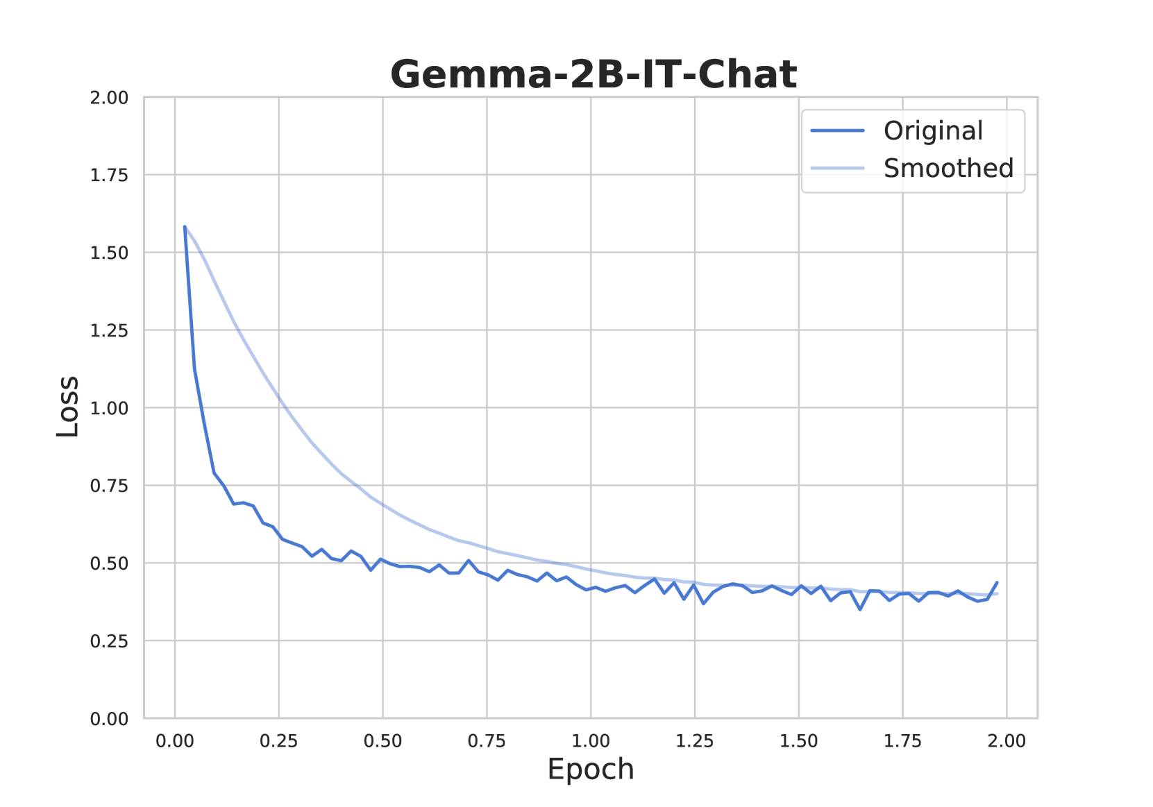Visual Description ## Line Chart: Gemma-2B-IT-Chat Loss vs. Epoch ### Overview This image presents a line chart illustrating the relationship between 'Loss' and 'Epoch' during the training of the Gemma-2B-IT-Chat model. Two lines are plotted: 'Original' and 'Smoothed', representing the loss function's behavior over training epochs. The chart aims to visualize the model's learning progress and stability. ### Components/Axes * **Title:** Gemma-2B-IT-Chat * **X-axis:** Epoch (ranging from approximately 0.00 to 2.00) * **Y-axis:** Loss (ranging from approximately 0.00 to 2.00) * **Legend:** * 'Original' - Dark Blue Line * 'Smoothed' - Light Blue Line ### Detailed Analysis The chart displays two lines representing the loss function over epochs. **Original Line (Dark Blue):** The 'Original' line starts at approximately 1.60 Loss at Epoch 0.00. It exhibits a steep downward trend until approximately Epoch 0.25, where the Loss reaches around 0.60. From Epoch 0.25 to Epoch 1.00, the line continues to decrease, but at a slower rate, reaching a minimum Loss of approximately 0.35 at Epoch 0.75. After Epoch 1.00, the line fluctuates between approximately 0.35 and 0.50, showing some instability. At Epoch 2.00, the Loss is approximately 0.40. **Smoothed Line (Light Blue):** The 'Smoothed' line begins at approximately 1.60 Loss at Epoch 0.00, mirroring the 'Original' line. It also shows a rapid decrease initially, reaching around 0.70 Loss at Epoch 0.25. The line continues to decline, leveling off around 0.40 Loss between Epochs 0.50 and 1.50. From Epoch 1.50 to Epoch 2.00, the line shows a slight increase, ending at approximately 0.45 Loss. **Data Points (Approximate):** | Epoch | Original Loss | Smoothed Loss | |-------|--------------|--------------| | 0.00 | 1.60 | 1.60 | | 0.25 | 0.60 | 0.70 | | 0.50 | 0.45 | 0.40 | | 0.75 | 0.35 | 0.35 | | 1.00 | 0.40 | 0.40 | | 1.25 | 0.45 | 0.40 | | 1.50 | 0.40 | 0.45 | | 1.75 | 0.40 | 0.45 | | 2.00 | 0.40 | 0.45 | ### Key Observations * Both lines demonstrate a decreasing trend in Loss, indicating that the model is learning over time. * The 'Smoothed' line provides a more stable representation of the learning process, reducing the impact of short-term fluctuations. * The 'Original' line exhibits more volatility after Epoch 1.00, suggesting potential overfitting or instability in the training process. * The loss appears to converge to a value around 0.40-0.45. ### Interpretation The chart illustrates the training dynamics of the Gemma-2B-IT-Chat model. The initial steep decline in Loss indicates rapid learning in the early stages of training. The subsequent leveling off and fluctuations suggest that the model is approaching a point of convergence, but may be experiencing some instability. The 'Smoothed' line helps to visualize the overall trend, filtering out noise and providing a clearer picture of the model's learning progress. The convergence around a loss of 0.40-0.45 suggests that the model has reached a reasonable level of performance on the training data. The fluctuations in the 'Original' line after Epoch 1.00 could indicate the need for regularization techniques or further hyperparameter tuning to prevent overfitting and improve generalization. The chart is a standard visualization for monitoring the training process of machine learning models, providing insights into their learning behavior and potential issues. </details> Figure 11: Fine-tuning loss plots for Gemma-2B-IT-Chat. | Parameter Base Model ROUGE-L | Value google/gemma-2b-it 0.667 | | --- | --- | | ROUGE-1 | 0.692 | | Fine-Tuning Type | LoRA | | LoRA Alpha | 16 | | LoRA Rank | 8 | | Cutoff Length | 4096 | | Gradient Accumulation Steps | 8 | | Learning Rate | 5.0e-05 | | LR Scheduler Type | Cosine | | Number of Training Epochs | 2.0 | | Optimizer | AdamW | | Quantization Bit | 4 | Table 12: Fine-tuning Parameters for Gemma-2B-IT-Chat **Text Span Attribution Verification** **Objective:** Predict whether the text span is "Attributable", "Contradictory", or "Extrapolatory" based on the information provided in the triplets. **Instructions:** 1. **Read the Full Text:** - Understand the context and content of the full text string. 2. **Examine the Text Span:** - Determine the claims made within the text span. 3. **Analyze the Triplets:** - Evaluate if the triplets support, refute, or neither support nor refute the claims in the text span. 4. **Make Your Prediction:** - Classify the text span as "Attributable", "Contradictory", or "Extrapolatory" based on your analysis of the triplets. 5. **Provide Rationale:** - Clearly explain your reasoning for the classification. **Classification Criteria:** - **"Attributable"**: The text span is sufficiently supported by the triplet(s). All claims in the text span are directly present in the triplet information. - **"Contradictory"**: The text span is conclusively refuted by the triplet(s). All claims in the text span are directly contradicted by the triplet information. - **"Extrapolatory"**: The triplet(s) can neither support nor refute the text span. The information provided is either irrelevant, indirect, or related but not sufficient to support or refute the text span. **Example:** **Full Text:** "Albert Einstein is widely recognized as the father of modern physics. He was awarded the Nobel Prize in Physics for his services to Theoretical Physics." **Text Span:** "He was awarded the Nobel Prize in Physics." **Triplets:** [("Albert Einstein", "award received", "Nobel Prize in Physics")] **Sample Evaluation:** - **Prediction:** "Attributable" - **Rationale:** "The triplet directly supports the claim that Albert Einstein received the Nobel Prize in Physics." **Example:** **Full Text:** "Isaac Newton discovered the element radium." **Text Span:** "Isaac Newton discovered radium." **Triplets:** [("Marie Curie", "discovered", "radium")] **Sample Evaluation:** - **Prediction:** "Contradictory" - **Rationale:** "The triplet states that Marie Curie discovered radium, contradicting the claim that Isaac Newton discovered it." **Example:** **Full Text:** "The Eiffel Tower is a wrought-iron lattice tower that was opened in 1889." **Text Span:** "The Eiffel Tower is a wrought-iron lattice tower that was opened in 1889." **Triplets:** [("Eiffel Tower", "located in", "Paris")] **Sample Evaluation:** - **Prediction:** "Extrapolatory" - **Rationale:** "The triplet states that the Eiffel Tower is located in Paris, which is related but not sufficient to confirm or refute that it was opened in 1889." **Verification Checklist:** - [ ] The prediction accurately reflects the relationship between the text span and the triplets. - [ ] The rationale clearly explains the classification based on the triplets. - [ ] The explanation is free from irrelevant information. **Response Format:** Provide your evaluation in the following JSON format: - "prediction": "Attributable", "Contradictory", or "Extrapolatory" - "rationale": "Your comments here" **Inputs to Evaluate** **Full text:** "{full_text}" **Text span:** "{text_span}" **Triplets:** {triplets} Figure 12: Prompt for the text span attribution verification task, guiding the model to classify text spans as "Attributable," "Contradictory," or "Extrapolatory" based on the provided triplets. The prompt design incorporates concepts such as few-shot learning, chain-of-thought reasoning Kojima et al. (2022), and tailored prompt engineering OpenAI (2024); Nori et al. (2023)