# Octree-GS: Towards Consistent Real-time Rendering with LOD-Structured 3D Gaussians
**Authors**: Kerui Ren, Lihan Jiang, Tao Lu, Mulin Yu, Linning Xu, Zhangkai Ni, Bo Dai
> K. Ren is with Shanghai Jiao Tong University and Shanghai AI Laboratory. E-mail: renkerui@sjtu.edu.cn.L. Jiang is with The University of Science and Technology of China and Shanghai AI Laboratory. E-mail: jianglihan@mail.ustc.edu.cn.T. Lu is with Brown University. E-mail: tao_lu@brown.edu.B. Dai and M. Yu are with Shanghai AI Laboratory. E-mails: doubledaibo@gmail.com, yumulin@pjlab.org.cn.L. Xu is with The Chinese University of Hong Kong. E-mail: linningxu@link.cuhk.edu.hk.Z. Ni is with Tongji University.∗*∗Equal contribution.††{\dagger}†Corresponding author.
Abstract
The recently proposed 3D Gaussian Splatting (3D-GS) demonstrates superior rendering fidelity and efficiency compared to NeRF-based scene representations. However, it struggles in large-scale scenes due to the high number of Gaussian primitives, particularly in zoomed-out views, where all primitives are rendered regardless of their projected size. This often results in inefficient use of model capacity and difficulty capturing details at varying scales. To address this, we introduce Octree-GS, a Level-of-Detail (LOD) structured approach that dynamically selects appropriate levels from a set of multi-scale Gaussian primitives, ensuring consistent rendering performance. To adapt the design of LOD, we employ an innovative grow-and-prune strategy for densification and also propose a progressive training strategy to arrange Gaussians into appropriate LOD levels. Additionally, our LOD strategy generalizes to other Gaussian-based methods, such as 2D-GS and Scaffold-GS, reducing the number of primitives needed for rendering while maintaining scene reconstruction accuracy. Experiments on diverse datasets demonstrate that our method achieves real-time speeds, with even 10 $×$ faster than state-of-the-art methods in large-scale scenes, without compromising visual quality. Project page: https://city-super.github.io/octree-gs/.
Index Terms: Novel View Synthesis, 3D Gaussian Splatting, Consistent Real-time Rendering, Level-of-Detail
<details>
<summary>x1.png Details</summary>
### Visual Description
## Rendering Comparison: Scaffold-GS, Octree-GS, and Hierarchical-GS
### Overview
The image presents a comparative analysis of three rendering techniques: Scaffold-GS, Octree-GS, and Hierarchical-GS. The image is divided into two rows. The top row displays rendered images of cityscapes using each of the three techniques. The bottom row shows the corresponding Gaussian Primitive representations. Each column represents a different scene. Performance metrics (FPS and #GS(M)) are provided below each Gaussian Primitive representation.
### Components/Axes
* **Rows:**
* Row 1: Rendering
* Row 2: Gaussian Primitives
* **Columns:** Each set of three columns represents a different scene. Within each set, the columns are:
* Column 1: Scaffold-GS
* Column 2: Octree-GS
* Column 3: Hierarchical-GS
* **Metrics:** Frames Per Second (FPS) and Number of Gaussian Splats in Millions (#GS(M))
### Detailed Analysis or ### Content Details
**Scene 1 (Leftmost Set of Columns):**
* **Rendering (Top Row):**
* **Scaffold-GS:** Shows a cityscape with buildings and roads. A red arrow points to a specific building.
* **Octree-GS:** Shows the same cityscape, rendered with a different technique.
* **Hierarchical-GS:** Shows the same cityscape, rendered with a different technique.
* **Gaussian Primitives (Bottom Row):**
* **Scaffold-GS:** A point cloud representation of the cityscape.
* 20.3 FPS / 3.20 #GS(M)
* **Octree-GS:** A point cloud representation of the cityscape.
* 48.5 FPS / 1.25 #GS(M)
* **Hierarchical-GS:** A point cloud representation of the cityscape.
* 11.9 FPS / 2.21 #GS(M)
**Scene 2 (Middle Set of Columns):**
* **Rendering (Top Row):**
* **Scaffold-GS:** Shows a cityscape with buildings and roads. A red arrow points to a specific building.
* **Octree-GS:** Shows the same cityscape, rendered with a different technique.
* **Hierarchical-GS:** Shows the same cityscape, rendered with a different technique.
* **Gaussian Primitives (Bottom Row):**
* **Scaffold-GS:** A point cloud representation of the cityscape.
* 8.68 FPS / 13.0 #GS(M)
* **Octree-GS:** A point cloud representation of the cityscape.
* 31.1 FPS / 3.21 #GS(M)
* **Hierarchical-GS:** A point cloud representation of the cityscape.
* 13.5 FPS / 4.91 #GS(M)
**Scene 3 (Rightmost Set of Columns):**
* **Rendering (Top Row):**
* **Scaffold-GS:** Shows a cityscape with buildings and roads. A red arrow points to a specific building.
* **Octree-GS:** Shows the same cityscape, rendered with a different technique.
* **Hierarchical-GS:** Shows the same cityscape, rendered with a different technique.
* **Gaussian Primitives (Bottom Row):**
* **Scaffold-GS:** A point cloud representation of the cityscape.
* 6.91 FPS / 20.8 #GS(M)
* **Octree-GS:** A point cloud representation of the cityscape.
* 32.0 FPS / 3.59 #GS(M)
* **Hierarchical-GS:** A point cloud representation of the cityscape.
* 16.5 FPS / 4.51 #GS(M)
### Key Observations
* The Octree-GS method generally achieves higher FPS compared to Scaffold-GS and Hierarchical-GS, especially in the first scene.
* The #GS(M) values vary significantly across the different methods and scenes, indicating different levels of detail or complexity in the Gaussian Splat representations.
* The red arrows in the renderings highlight specific areas of interest within each scene.
### Interpretation
The image provides a visual and quantitative comparison of three Gaussian Splatting rendering techniques. The data suggests that Octree-GS may offer a better balance between rendering speed (FPS) and the number of Gaussian Splats used (#GS(M)) in some scenarios. However, the optimal technique likely depends on the specific scene and desired level of detail. The Gaussian Primitive representations in the bottom row offer insight into how each method distributes and represents the scene's geometry. The red arrows likely indicate areas where the rendering quality or performance of the different methods is being specifically compared.
</details>
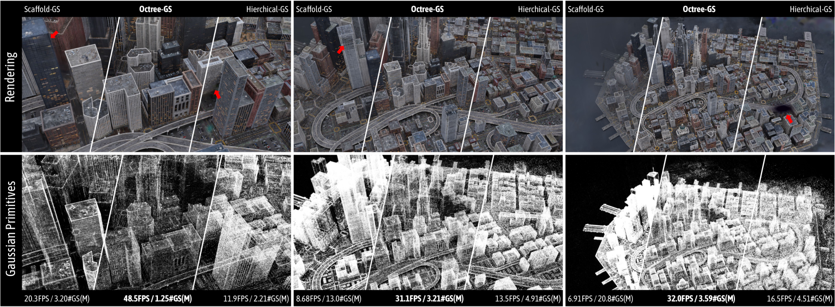
Figure 1: Visualization of a continuous zoom-out trajectory on the MatrixCity [1] dataset. Both the rendered 2D images and the corresponding Gaussian primitives are indicated. As indicated by the highlighted arrows, Octree-GS consistently demonstrates superior visual quality compared to state-of-the-art methods Hierarchical-GS [2] and Scaffold-GS [3]. Both SOTA methods fail to render the excessive number of Gaussian primitives included in distant views in real-time, whereas Octree-GS consistently achieves real-time rendering performance ( $≥ 30$ FPS). First row metrics: FPS/storage size.
I Introduction
The field of novel view synthesis has seen significant advancements driven by the advancement of radiance fields [4], which deliver high-fidelity rendering. However, these methods often suffer from slow training and rendering speeds due to time-consuming stochastic sampling. Recently, 3D Gaussian splatting (3D-GS) [5] has pushed the field forward by using anisotropic Gaussian primitives, achieving near-perfect visual quality with efficient training times and tile-based splatting techniques for real-time rendering. With such strengths, it has significantly accelerated the process of replicating the real world into a digital counterpart [6, 7, 8, 9], igniting the community’s imagination for scaling real-to-simulation environments [10, 11, 3]. With its exceptional visual effects, an unprecedented photorealistic experience in VR/AR [12, 13] is now more attainable than ever before.
A key drawback of 3D-GS [5] is the misalignment between the distribution of 3D Gaussians and the actual scene structure. Instead of aligning with the geometry of the scene, the Gaussian primitives are distributed based on their fit to the training views, leading to inaccurate and inefficient placement. This misalignment causes two bottleneck challenges: 1) it reduces robustness in rendering views that differ significantly from the training set, as the primitives are not optimized for generalization, and 2) results in redundant and overlap primitives that fail to efficiently represent scene details for real-time rendering, especially in large-scale urban scenes with millions of primitives.
There are variants of the vanilla 3D-GS [5] that aim at resolving the misalignment between the organization of 3D Gaussians and the structure of target scene. Scaffold-GS [3] enhances the structure alignment by introducing a regularly spaced feature grid as a structural prior, improving the arrangement and viewpoint-aware adjustment of Gaussians for better rendering quality and efficiency. Mip-Splatting [14] resorts to 3D smoothing and 2D Mip filters to alleviate the redundancy of 3D Gaussians during the optimiziation process of 3D-GS. 2D-GS [15] forces the primitives to better align with the surface, enabling faster reconstruction.
Although the aforementioned improvements have been extensively tested on diverse public datasets, we identify a new challenge in the Gaussian era: recording large-scale scenes is becoming increasingly common, yet these methods inherently struggles to scale, as shown in Fig 1. This limitation arises because they still rely on visibility-based filtering for primitive selection, considering all primitives within the view frustum without accounting for their projected sizes. As a result, every object detail is rendered, regardless of distance, leading to redundant computations and inconsistent rendering speeds, particularly in zoom-out scenarios involving large, complex scenes. The lack of Level-of-Detail (LOD) adaptation further forces all 3D Gaussians to compete across views, degrading rendering quality at different scales. As scene complexity increases, the growing number of Gaussians amplifies bottlenecks in real-time rendering.
To address the aforementioned issues and better accommodate the new era, we integrate an octree structure into the Gaussian representation, inspired by previous works [16, 17, 18] that demonstrate the effectiveness of spatial structures like octrees and multi-resolution grids for flexible content allocation and real-time rendering. Specifically, our method organizes scenes with hierarchical grids to meet LOD needs, efficiently adapting to complex or large-scale scenes during both training and inference, with LOD levels selected based on observation footprint and scene detail richness. We further employ a progressive training strategy, introducing a novel growing and pruning approach. A next-level growth operator enhances connections between LODs, increasing high-frequency detail, while redundant Gaussians are pruned based on opacity and view frequency. By adaptively querying LOD levels from the octree-based Gaussian structure based on viewing distance and scene complexity, our method minimizes the number of primitives needed for rendering, ensuring consistent efficiency, as shown in Fig. 1. In addition, Octree-GS effectively separates coarse and fine scene details, allowing for accurate Gaussian placement at appropriate scales, significantly improving reconstruction fidelity and texture detail.
Unlike other concurrent LOD methods [2, 19], our approach is an end-to-end algorithm that achieves LOD effects in a single training round, reducing training time and storage overhead. Notably, our LOD framework is also compatible with various Gaussian representations, including explicit Gaussians [15, 5] and neural Gaussians [3]. By incorporating our strategy, we have demonstrated significant enhancements in visual performance and rendering speed across a wide range of datasets, including both fine-detailed indoor scenes and large-scale urban environments.
In summary, our method offers the following key contributions:
- To the best of our knowledge, Octree-GS is the first approach to deal with the problem of Level-of-Detail in Gaussian representation, enabling consistent rendering speed by dynamically adjusting the fetched LOD on-the-fly owing to our explicit octree structure design.
- We develop a novel grow-and-prune strategy optimized for LOD adaptation.
- We introduce a progressive training strategy to encourage more reliable distributions of primitives.
- Our LOD strategy is able to generalize to any Gaussian-based method.
- Our methods, while maintaining the superior rendering quality, achieves state-of-the-art rendering speed, especially in large-scale scenes and extreme-view sequences, as shown in Fig. 1.
II Related work
II-A Novel View Synthesis
NeRF methods [4] have revolutionized the novel view synthesis task with their photorealistic rendering and view-dependent modeling effects. By leveraging classical volume rendering equations, NeRF trains a coordinate-based MLP to encode scene geometry and radiance, mapping directly from positionally encoded spatial coordinates and viewing directions. To ease the computational load of dense sampling process and forward through deep MLP layers, researchers have resorted to various hybrid-feature grid representations, akin to ‘caching’ intermediate latent features for final rendering [20, 17, 21, 22, 23, 24, 25, 26]. Multi-resolution hash encoding [24] is commonly chosen as the default backbone for many recent advancements due to its versatility for enabling fast and efficient rendering, encoding scene details at various granularities [27, 28, 29] and extended supports for LOD renderings [16, 30].
Recently, 3D-GS [5] has ignited a revolution in the field by employing anisotropic 3D Gaussians to represent scenes, achieving state-of-the-art rendering quality and speed. Subsequent studies have rapidly expanded 3D-GS into diverse downstream applications beyond static 3D reconstruction, sparking a surge of extended applications to 3D generative modeling [31, 32, 33], physical simulation [13, 34], dynamic modeling [35, 36, 37], SLAMs [38, 39], and autonomous driving scenes [12, 10, 11], etc. Despite the impressive rendering quality and speed of 3D-GS, its ability to sustain stable real-time rendering with rich content is hampered by the accompanying rise in resource costs. This limitation hampers its practicality in speed-demanding applications, such as gaming in open-world environments and other immersive experiences, particularly for large indoor and outdoor scenes with computation-restricted devices.
II-B Spatial Structures for Neural Scene Representations
Various spatial structures have been explored in previous NeRF-based representations, including dense voxel grids [20, 22], sparse voxel grids [17, 21], point clouds [40], multiple compact low-rank tensor components [23, 41, 42], and multi-resolution hash tables [24]. These structures primarily aim to enhance training or inference speed and optimize storage efficiency. Inspired by classical computer graphics techniques such as BVH [43] and SVO [44] which are designed to model the scene in a sparse hierarchical structure for ray tracing acceleration. NSVF [20] efficiently skipping the empty voxels leveraging the neural implicit fields structured in sparse octree grids. PlenOctree [17] stores the appearance and density values in every leaf to enable highly efficient rendering. DOT [45] improves the fixed octree design in Plenoctree with hierarchical feature fusion. ACORN [18] introduces a multi-scale hybrid implicit–explicit network architecture based on octree optimization.
While vanilla 3D-GS [5] imposes no restrictions on the spatial distribution of all 3D Gaussians, allowing the modeling of scenes with a set of initial sparse point clouds, Scaffold-GS [3] introduces a hierarchical structure, facilitating more accurate and efficient scene reconstruction. In this work, we introduce a sparse octree structure to Gaussian primitives, which demonstrates improved capabilities such as real-time rendering stability irrespective of trajectory changes.
II-C Level-of-Detail (LOD)
LOD is widely used in computer graphics to manage the complexity of 3D scenes, balancing visual quality and computational efficiency. It is crucial in various applications, including real-time graphics, CAD models, virtual environments, and simulations. Geometry-based LOD involves simplifying the geometric representation of 3D models using techniques like mesh decimation; while rendering-based LOD creates the illusion of detail for distant objects presented on 2D images. The concept of LOD finds extensive applications in geometry reconstruction [46, 47, 48] and neural rendering [49, 50, 30, 27, 16]. Mip-NeRF [49] addresses aliasing artifacts by cone-casting approach approximated with Gaussians. BungeeNeRF [51] employs residual blocks and inclusive data supervision for diverse multi-scale scene reconstruction. To incorporate LOD into efficient grid-based NeRF approaches like instant-NGP [24], Zip-NeRF [30] further leverages supersampling as a prefiltered feature approximation. VR-NeRF [16] utilizes mip-mapping hash grid for continuous LOD rendering and an immersive VR experience. PyNeRF [27] employs a pyramid design to adaptively capture details based on scene characteristics. However, GS-based LOD methods fundamentally differ from above LOD-aware NeRF methods in scene representation and LOD introduction. For instance, NeRF can compute LOD from per-pixel footprint size, whereas GS-based methods require joint LOD modeling from both the view and 3D scene level. We introduce a flexible octree structure to address LOD-aware rendering in the 3D-GS framework.
Concurrent works related to our method include LetsGo [52], CityGaussian [19], and Hierarchical-GS [2], all of which also leverage LOD for large-scale scene reconstruction. 1) LetsGo introduces multi-resolution Gaussian models optimized jointly, focusing on garage reconstruction, but requires multi-resolution point cloud inputs, leading to higher training overhead and reliance on precise point cloud accuracy, making it more suited for lidar scanning scenarios. 2) CityGaussian selects LOD levels based on distance intervals and fuses them for efficient large-scale rendering, but lacks robustness due to the need for manual distance threshold adjustments, and faces issues like stroboscopic effects when switching between LOD levels. 3) Hierarchical-GS, using a tree-based hierarchy, shows promising results in street-view scenes but involves post-processing for LOD, leading to increased complexity and longer training times. A common limitation across these methods is that each LOD level independently represents the entire scene, increasing storage demands. In contrast, Octree-GS employs an explicit octree structure with an accumulative LOD strategy, which significantly accelerates rendering speed while reducing storage requirements.
III Preliminaries
In this section, we present a brief overview of the core concepts underlying 3D-GS [5] and Scaffold-GS [3].
III-A 3D-GS
3D Gaussian splatting [5] explicitly models scenes using anisotropic 3D Gaussians and renders images by rasterizing the projected 2D counterparts. Each 3D Gaussian $G(x)$ is parameterized by a center position $\mu∈\mathbb{R}^{3}$ and a covariance $\Sigma∈\mathbb{R}^{3× 3}$ :
$$
G(x)=e^{-\frac{1}{2}(x-\mu)^{T}\Sigma^{-1}(x-\mu)}, \tag{1}
$$
where $x$ is an arbitrary position within the scene, $\Sigma$ is parameterized by a scaling matrix $S∈\mathbb{R}^{3}$ and rotation matrix $R∈\mathbb{R}^{3× 3}$ with $RSS^{T}R^{T}$ . For rendering, opacity $\sigma∈\mathbb{R}$ and color feature $F∈\mathbb{R}^{C}$ are associated to each 3D Gaussian, while $F$ is represented using spherical harmonics (SH) to model view-dependent color $c∈\mathbb{R}^{3}$ . A tile-based rasterizer efficiently sorts the 3D Gaussians in front-to-back depth order and employs $\alpha$ -blending, following projecting them onto the image plane as 2D Gaussians $G^{\prime}(x^{\prime})$ [53]:
$$
C\left(x^{\prime}\right)=\sum_{i\in N}T_{i}c_{i}\sigma_{i},\quad\sigma_{i}=%
\alpha_{i}G_{i}^{\prime}\left(x^{\prime}\right), \tag{2}
$$
where $x^{\prime}$ is the queried pixel, $N$ represents the number of sorted 2D Gaussians binded with that pixel, and $T$ denotes the transmittance as $\prod_{j=1}^{i-1}\left(1-\sigma_{j}\right)$ .
III-B Scaffold-GS
To efficiently manage Gaussian primitives, Scaffold-GS [3] introduces anchors, each associated with a feature describing the local structure. From each anchor, $k$ neural Gaussians are emitted as follows:
$$
\left\{\mu_{0},\ldots,\mu_{k-1}\right\}=x_{v}+\left\{\mathcal{O}_{0},\ldots,%
\mathcal{O}_{k-1}\right\}\cdot l_{v} \tag{3}
$$
where $x_{v}$ is the anchor position, $\{\mu_{i}\}$ denotes the positions of the i th neural Gaussian, and $l_{v}$ is a scaling factor controlling the predicted offsets $\{\mathcal{O}_{i}\}$ . In addition, opacities, scales, rotations, and colors are decoded from the anchor features through corresponding MLPs. For example, the opacities are computed as:
$$
\{{\alpha}_{0},...,{\alpha}_{k-1}\}=\rm{F_{\alpha}}(\hat{f}_{v},\Delta_{vc},%
\vec{d}_{vc}), \tag{4}
$$
where $\{\alpha_{i}\}$ represents the opacity of the i th neural Gaussian, decoded by the opacity MLP $F_{\alpha}$ . Here, $\hat{f}_{v}$ , $\Delta_{vc}$ , and $\vec{d}_{vc}$ correspond to the anchor feature, the relative viewing distance, and the direction to the camera, respectively. Once these properties are predicted, neural Gaussians are fed into the tile-based rasterizer, as described in [5], to render images. During the densification stage, Scaffold-GS treats anchors as the basic primitives. New anchors are established where the gradient of a neural Gaussian exceeds a certain threshold, while anchors with low average transparency are removed. This structured representation improves robustness and storage efficiency compared to the vanilla 3D-GS.
IV Methods
<details>
<summary>x2.png Details</summary>
### Visual Description
## Diagram: Octree-GS Pipeline and Anchor Initialization
### Overview
The image presents a diagram illustrating the pipeline of Octree-GS and anchor initialization. It shows the process of generating a 3D representation from sparse SfM points, refining it through different Levels of Detail (LODs), and initializing anchors for further processing.
### Components/Axes
* **Sparse SfM Points:** A point cloud representation of a scene, likely generated using Structure from Motion (SfM) techniques.
* **Octree Structure:** A hierarchical tree structure used to partition 3D space, enabling efficient storage and processing of 3D data.
* **Camera Icon (O\*)**: Represents the camera's viewpoint.
* **LOD 0 anchors, +LOD 1, +LOD 2:** Different levels of detail for the 3D representation.
* **Rendering:** A rendered image of the 3D scene.
* **GT:** Ground Truth image of the scene.
* **L1, LSSIM, (Lvol, Ld, Ln):** Loss functions used for supervision.
* **bbox:** Bounding box.
* **LOD 0, LOD K-1:** Level of detail 0 and Level of detail K-1.
### Detailed Analysis
The diagram is divided into two main parts, labeled (a) and (b).
**(a) Pipeline of Octree-GS:**
1. **Sparse SfM Points:** The process begins with a sparse point cloud.
2. **Camera Viewpoint (O\*)**: An arrow indicates the camera's viewpoint.
3. **LOD Refinement:** The point cloud is refined through different levels of detail (LOD 0, +LOD 1, +LOD 2). The images show the progression of detail as the LOD increases.
4. **Rendering:** A rendered image is generated from the refined 3D representation. This rendering is enclosed in a green box.
5. **Ground Truth (GT):** A ground truth image of the scene is provided for comparison.
6. **Supervision Loss:** Loss functions (L1, LSSIM, (Lvol, Ld, Ln)) are used to supervise the training process.
The text "Fetch proper LODs based on views" is placed below the LOD refinement images, indicating that the appropriate level of detail is selected based on the viewpoint.
**(b) Anchor Initialization:**
1. **Construct the octree-structure grids:** The first step involves constructing octree grids within a bounding box (bbox).
2. **Initialize anchors with varying LOD levels:** Anchors are initialized with varying levels of detail, ranging from LOD 0 to LOD K-1.
### Key Observations
* The diagram illustrates a pipeline for generating and refining 3D representations from sparse point clouds.
* Octree structures and LODs are used to efficiently represent and process 3D data.
* Supervision loss functions are used to guide the training process.
* Anchor initialization is performed using varying LOD levels.
### Interpretation
The diagram describes a method for generating 3D representations of scenes from sparse point clouds. The Octree-GS pipeline uses octree structures and LODs to efficiently represent and process the 3D data. The anchor initialization process prepares the data for further processing, such as object detection or scene understanding. The use of supervision loss functions ensures that the generated 3D representations are accurate and consistent with the ground truth.
</details>
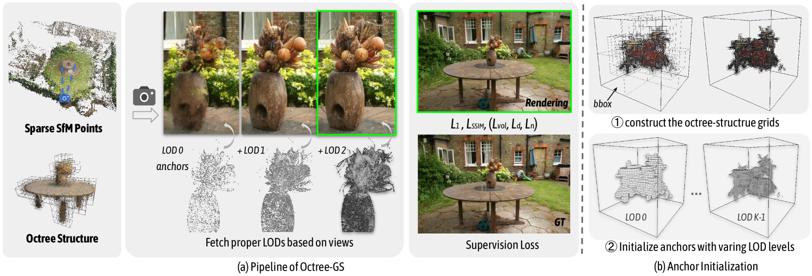
Figure 2: (a) Pipeline of Octree-GS: starting from given sparse SfM points, we construct octree-structured anchors from the bounded 3D space and assign them to the corresponding LOD level. Unlike conventional 3D-GS methods treating all Gaussians equally, our approach involves primitives with varying LOD levels. We determine the required LOD levels based on the observation view and invoke corresponding anchors for rendering, as shown in the middle. As the LOD levels increase (from LOD $0 0$ to LOD $2$ ), the fine details of the vase accumulate progressively. (b) Anchor Initialization: We construct the octree structure grids within the determined bounding box. Then, the anchors are initialized at the voxel center of each layer , with their LOD level corresponding to the octree layer of the voxel, ranging from $0 0$ to $K-1$ .
Octree-GS hierarchically organizes anchors into an octree structure to learn a neural scene from multiview images. Each anchor can emit different types of Gaussian primitives, such as explicit Gaussians [15, 5] and neural Gaussians [3]. By incorporating the octree structure, which naturally introduces a LOD hierarchy for both reconstruction and rendering, Octree-GS ensures consistently efficient training and rendering by dynamically selecting anchors from the appropriate LOD levels, allowing it to efficiently adapt to complex or large-scale scenes. Fig. 2 illustrates our framework.
In this section, we first explain how to construct the octree from a set of given sparse SfM [54] points in Sec. IV-A. Next, we introduce an adapted anchor densification strategy based on LOD-aware ‘growing’ and ‘pruning’ operations in Sec IV-B. Sec. IV-C then introduces a progressive training strategy that activates anchors from coarse to fine. Finally, to address reconstruction challenges in wild scenes, we introduce appearance embedding (Sec. IV-D).
IV-A LOD-structured Anchors
IV-A 1 Anchor Definition.
Inspired by Scaffold-GS [3], we introduce anchors to manage Gaussian primitives. These anchors are positioned at the centers of sparse, uniform voxel grids with varying voxel sizes. Specifically, anchors with higher LOD $L$ are placed within grids with smaller voxel sizes. In this paper, we define LOD 0 as the coarsest level. As the LOD level increases, more details are captured. Note that our LOD design is cumulative: the rendered images at LOD $K$ rasterize all Gaussian primitives from LOD $0 0$ to $K$ . Additionally, each anchor is assigned a LOD bias $\Delta L$ to account for local complexity, and each anchor is associated with $k$ Gaussian primitives for image rendering, whose positions are determined by Eq. 3. Moreover, our framework is generalized to support various types of Gaussians. For example, the Gaussian primitive can be explicitly defined with learnable distinct properties, such as 2D [15] or 3D Gaussians [5], or they can be neural Gaussians decoded from the corresponding anchors, as described in Sec. V-A 4.
IV-A 2 Anchor Initialization.
In this section, we describe the process of initializing octree-structured anchors from a set of sparse SfM points $\mathbf{P}$ . First, the number of octree layers, $K$ , is determined based on the range of observed distances. Specifically, we begin by calculating the distance $d_{ij}$ between each camera center of training image $i$ and SfM point $j$ . The $r_{d}$ th largest and $r_{d}$ th smallest distances are then defined as $d_{max}$ and $d_{min}$ , respectively. Here, $r_{d}$ is a hyperparameter used to discard outliers, which is typically set to $0.999$ in all our experiment. Finally, $K$ is calculated as:
$$
\displaystyle K \displaystyle=\lfloor\log_{2}(\hat{d}_{max}/\hat{d}_{min})\rceil+1. \tag{5}
$$
where $\lfloor·\rceil$ denotes the round operator. The octree-structured grids with $K$ layers are then constructed, and the anchors of each layer are voxelized by the corresponding voxel size:
$$
\mathbf{V}_{L}=\left\{\left\lfloor\frac{\mathbf{P}}{\delta/2^{L}}\right\rceil%
\cdot\delta/2^{L}\right\}, \tag{6}
$$
given the base voxel size $\delta$ for the coarsest layer corresponding to LOD 0 and $\mathbf{V}_{L}$ for initialed anchors in LOD $L$ . The properties of anchors and the corresponding Gaussian primitives are also initialized, please check the implementation V-A 4 for details.
IV-A 3 Anchor Selection.
In this section, we explain how to select the appropriate visible anchors to maintain both stable real-time rendering speed and high rendering quality. An ideal anchors is dynamically fetched from $K$ LOD levels based on the pixel footprint of projected Gaussians on the screen. In practice, we simplify this by using the observation distance $d_{ij}$ , as it is proportional to the footprint under consistent camera intrinsics. For varying intrinsics, a focal scale factor $s$ is applied to adjust the distance equivalently. However, we find it sub-optimal if we estimate the LOD level solely based on observation distances. So we further set a learnable LOD bias $\Delta L$ for each anchor as a residual, which effectively supplements the high-frequency regions with more consistent details to be rendered during inference process, such as the presented sharp edges of an object as shown in Fig. 13. In detail, for a given viewpoint $i$ , the corresponding LOD level of an arbitrary anchor $j$ is estimated as:
$$
\hat{L_{ij}}=\lfloor L_{ij}^{*}\rfloor=\lfloor\Phi(\log_{2}(d_{max}/(d_{ij}*s)%
))+\Delta L_{j}\rfloor, \tag{7}
$$
where $d_{ij}$ is the distance between viewpoint $i$ and anchor $j$ . $\Phi(·)$ is a clamping function that restricts the fractional LOD level $L_{ij}^{*}$ to the range $[0,K-1]$ . Inspired by the progressive LOD techniques [55], Octree-GS renders images using cumulative LOD levels rather than a single LOD level. In summary, the anchor will be selected if its LOD level $L_{j}≤\hat{L_{ij}}$ . We iteratively evaluate all anchors and select those that meet this criterion, as illustrated in Fig. 3. The Gaussian primitives emitted from the selected anchors are then passed into the rasterizer for rendering.
During inference, to ensure smooth rendering transitions between different LOD levels without introducing visible artifacts, we adopt an opacity blending technique inspired by [16, 51]. We use piecewise linear interpolation between adjacent levels to make LOD transitions continuous, effectively eliminating LOD aliasing. Specifically, in addition to fully satisfied anchors, we also select nearly satisfied anchors that meet the criterion $L_{j}=\hat{L_{ij}}+1$ . The Gaussian primitives of these anchors are also passed to the rasterizer, with their opacities scaled by $L_{ij}^{*}-\hat{L_{ij}}$ .
IV-B Adaptive Anchor Gaussians Control
IV-B 1 Anchor Growing.
Following the approach of [5], we use the view-space positional gradients of Gaussian primitives as a criterion to guide anchor densification. New anchors are grown in the unoccupied voxels across the octree-structured grids, following the practice of [3]. Specifically, every $T$ iterations, we calculate the average accumulated gradient of the spawned Gaussian primitives, denoted as $∇_{g}$ . Gaussian primitives with $∇_{g}$ exceeding a predefined threshold $\tau_{g}$ are considered significant and they are converted into new anchors if located in empty voxels. In the context of the octree structure, the question arises: which LOD level should be assigned to these newly converted anchors? To address this, we propose a ‘next-level’ growing operation. This method adjusts the growing strategy by adding new anchors at varying granularities, with Gaussian primitives that have exceptionally high gradients being promoted to higher levels. To prevent overly aggressive growth into higher LOD levels, we monotonically increase the difficulty of growing new anchors to higher LOD levels by setting the threshold $\tau_{g}^{L}=\tau_{g}*2^{\beta L}$ , where $\tau_{g}$ and $\beta$ are both hyperparameters, with default values of $0.0002$ and $0.2$ , respectively. Gaussians at level $L$ are only promoted to the next level $L+1$ if $∇_{g}>\tau_{g}^{L+1}$ , and they remain at the same level if $\tau_{g}^{L}<∇_{g}<\tau_{g}^{L+1}$ .
We also utilize the gradient as the complexity cue of the scene to adjust the LOD bias $\Delta L$ . The gradient of an anchor is defined as the average gradient of the spawned Gaussian primitives, denoted as $∇_{v}$ . We select those anchors with $∇_{v}>\tau_{g}^{L}*0.25$ , and increase the corresponding $\Delta L$ by a small user-defined quantity $\epsilon$ : $\Delta L=\Delta L+\epsilon$ . We empirically set $\epsilon=0.01$ .
<details>
<summary>x3.png Details</summary>
### Visual Description
## Image Comparison: Progressive LOD vs. Non-Progressive LOD
### Overview
The image presents a visual comparison of rendering scenes with and without progressive Level of Detail (LOD) loading. It showcases how the scene's appearance changes with increasing LOD levels (0, 3, 4, and 5) under two different rendering approaches: one using progressive loading and the other without. The scene on the left depicts a rainy street with a car, while the scenes on the right depict a truck. Each scene is split diagonally, with the top half rendered with progressive loading and the bottom half without.
### Components/Axes
* **Rows:** Two rows, labeled "w/ progressive" (top row) and "w/o progressive" (bottom row).
* **Columns:** Four columns representing different LOD levels: LOD 0, LOD 3, LOD 4, and LOD 5.
* **Diagonal Division:** Each image is divided diagonally from the bottom-left to the top-right. The top-left triangle shows the scene rendered with progressive loading, while the bottom-right triangle shows the scene rendered without progressive loading.
* **Bounding Boxes:** Green dashed bounding boxes highlight a specific region in the "w/ progressive" images. Red dashed bounding boxes highlight a specific region in the "w/o progressive" images.
### Detailed Analysis
**Column 1: LOD 0**
* **Scene:** Rainy street with a car.
* **w/ progressive (top-left):** The top-left triangle shows a noisy, sparse point cloud representation of the scene.
* **w/o progressive (bottom-right):** The bottom-right triangle shows a blurred, low-resolution image of the scene.
**Column 2: LOD 3**
* **Scene:** Truck.
* **w/ progressive (top-left):** The top-left triangle shows a more defined point cloud representation of the truck, with some details visible.
* **w/o progressive (bottom-right):** The bottom-right triangle shows a more defined image of the truck, with some details visible.
**Column 3: LOD 4**
* **Scene:** Truck.
* **w/ progressive (top-left):** The top-left triangle shows a further refined point cloud representation of the truck, with more details visible.
* **w/o progressive (bottom-right):** The bottom-right triangle shows a more refined image of the truck, with more details visible.
**Column 4: LOD 5**
* **Scene:** Truck.
* **w/ progressive (top-left):** The top-left triangle shows a highly detailed point cloud representation of the truck.
* **w/o progressive (bottom-right):** The bottom-right triangle shows a highly detailed image of the truck.
### Key Observations
* **Progressive Loading:** The "w/ progressive" row demonstrates how the scene gradually refines as the LOD level increases. The initial representation (LOD 0) is a sparse point cloud, which becomes denser and more detailed with higher LOD levels.
* **Non-Progressive Loading:** The "w/o progressive" row shows how the scene appears only when the specified LOD level is fully loaded. The initial representation (LOD 0) is a low-resolution blur, which becomes sharper and more detailed with higher LOD levels.
* **Visual Difference:** The diagonal split highlights the difference between the two approaches at each LOD level. Progressive loading provides an initial representation of the scene quickly, which is then refined over time. Non-progressive loading waits until the specified LOD level is fully loaded before displaying the scene.
### Interpretation
The image illustrates the trade-offs between progressive and non-progressive LOD loading. Progressive loading offers a faster initial rendering, allowing users to see a basic representation of the scene quickly. This is useful for interactive applications where responsiveness is important. Non-progressive loading, on the other hand, provides a higher-quality rendering once the specified LOD level is fully loaded. This is suitable for applications where visual fidelity is paramount, and initial loading time is less of a concern. The choice between the two approaches depends on the specific requirements of the application and the desired user experience.
</details>
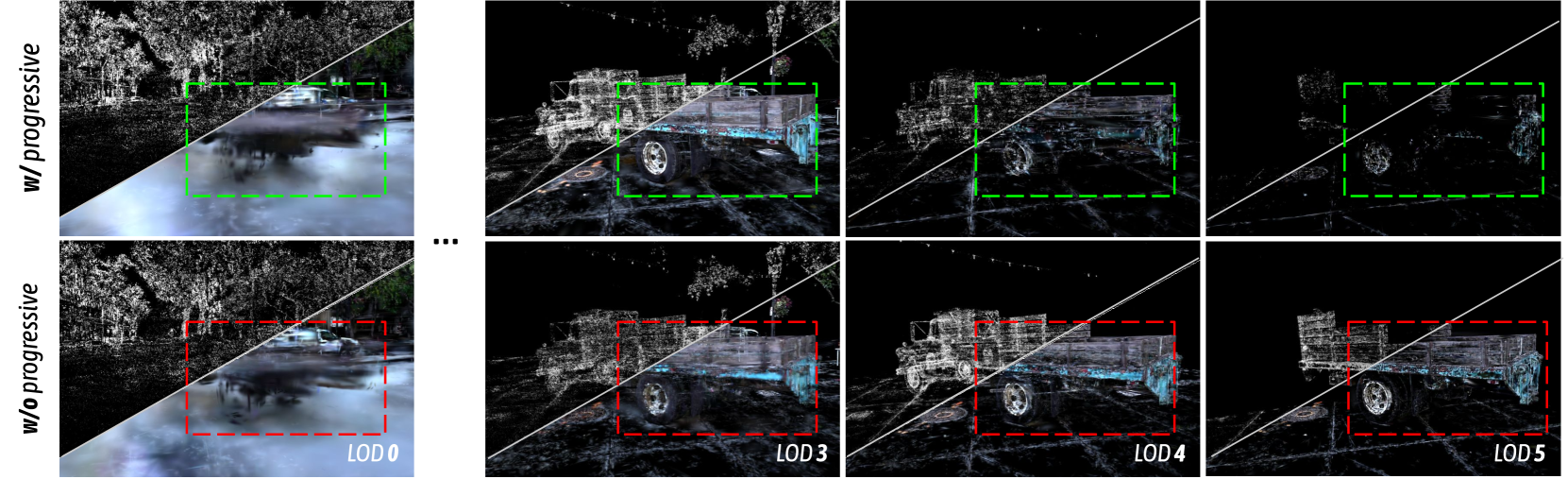
Figure 3: Visualization of anchors and projected 2D Gaussians in varying LOD levels. (1) The first row depicts scene decomposition with our full model, employing a coarse-to-fine training strategy as detailed in Sec. IV-C. A clear division of roles is evident between varying LOD levels: LOD 0 captures most rough contents, and higher LODs gradually recover the previously missed high-frequency details. This alignment with our motivation allows for more efficient allocation of model capacity with an adaptive learning process. (2) In contrast, our ablated progressive training studies (elaborated in Sec. V-C) take a naive approach. Here, all anchors are simultaneously trained, leading to an entangled distribution of Gaussian primitives across all LOD levels.
IV-B 2 Anchor Pruning.
To eliminate redundant and ineffective anchors, we compute the average opacity of Gaussians generated over $T$ training iterations, in a manner similar to the strategies adopted in [3].
<details>
<summary>x4.png Details</summary>
### Visual Description
## Image Comparison: Rendering with and without View Frequency
### Overview
The image presents a side-by-side comparison of three renderings of a scene depicting foliage. The renderings are labeled (a), (b), and (c). (a) shows a rendering without view frequency, (b) shows LOD (Level of Detail) levels without view frequency, and (c) shows a rendering with view frequency. Each rendering includes a smaller and larger rectangular region highlighted, with associated dB and G values.
### Components/Axes
* **(a) Rendering (w/o view frequency):** Image of foliage with a red rectangle highlighting a small region in the top-left and a larger region in the center. Text "27.51dB/1.16G" is present in the bottom-right corner of the image.
* **(b) LOD levels (w/o view frequency):** Grayscale image of foliage with a red rectangle highlighting a small region in the top-left and a larger region in the center.
* **(c) Rendering (w/ view frequency):** Image of foliage with a green rectangle highlighting a small region in the top-left and a larger region in the center. Text "27.63dB/0.24G" is present in the bottom-right corner of the image.
### Detailed Analysis or Content Details
* **Rendering (w/o view frequency) (a):**
* The image shows a scene of green foliage.
* A smaller red rectangle is located in the top-left portion of the image, highlighting a specific area.
* A larger red rectangle is located in the center of the image, highlighting a larger area.
* The text "27.51dB/1.16G" is displayed in the bottom-right corner.
* **LOD levels (w/o view frequency) (b):**
* The image is in grayscale, showing the level of detail.
* A smaller red rectangle is located in the top-left portion of the image, highlighting a specific area.
* A larger red rectangle is located in the center of the image, highlighting a larger area.
* **Rendering (w/ view frequency) (c):**
* The image shows a scene of green foliage.
* A smaller green rectangle is located in the top-left portion of the image, highlighting a specific area.
* A larger green rectangle is located in the center of the image, highlighting a larger area.
* The text "27.63dB/0.24G" is displayed in the bottom-right corner.
### Key Observations
* The image compares rendering with and without view frequency.
* The LOD levels image is in grayscale.
* The dB value is slightly higher for the rendering with view frequency (27.63dB) compared to the rendering without view frequency (27.51dB).
* The G value is significantly lower for the rendering with view frequency (0.24G) compared to the rendering without view frequency (1.16G).
### Interpretation
The image demonstrates the impact of view frequency on rendering. The LOD levels image shows the detail levels without color information. The dB values likely represent a measure of image quality (higher is better), while the G values likely represent the computational cost or memory usage (lower is better). The rendering with view frequency achieves a slightly better image quality with a significantly lower computational cost, suggesting that incorporating view frequency is an efficient rendering technique.
</details>
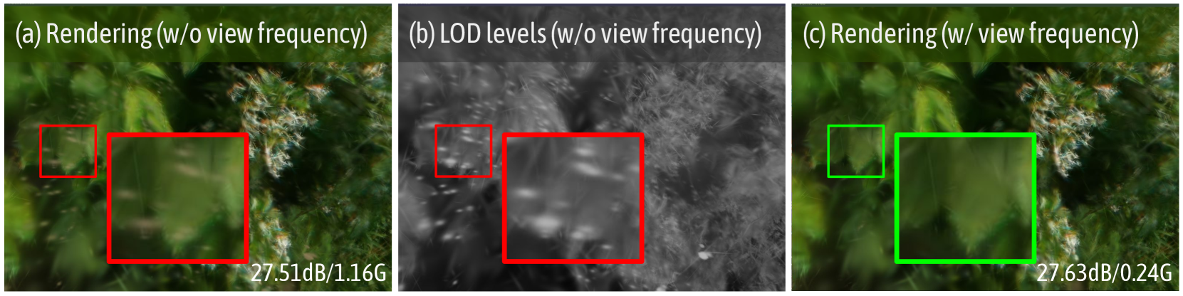
Figure 4: Illustration of the effect of view frequency. We visualize the rendered image and the corresponding LOD levels (with whiter colors indicating higher LOD levels) from a novel view. We observe that insufficiently optimized anchors will produce artifacts if pruning is based solely on opacity. After pruning anchors based on view frequency, not only are the artifacts eliminated, but the final storage is also reduced. Last row metrics: PSNR/storage size.
Moreover, we observe that some intolerable floaters appear in Fig. 4 (a) because a significant portion of anchors are not visible or selected in most training view frustums. Consequently, they are not sufficiently optimized, impacting rendering quality and storage overhead significantly. To address this issue, we define ‘view-frequency’ as the probability that anchors are selected in the training views, which directly correlates with the received gradient. We remove anchors with the view-frequency below $\tau_{v}$ , where $\tau_{v}$ represents the visibility threshold. This strategy effectively eliminates floaters, improving visual quality and significantly reducing storage, as demonstrated in Fig. 4.
IV-C Progressive Training
Optimizing anchors across all LOD levels simultaneously poses inherent challenges in explaining rendering with decomposed LOD levels. All LOD levels try their best to represent the 3D scene, making it difficult to decompose them thus leading to large overlaps.
Inspired by the progressive training strategy commonly used in prior NeRF methods [56, 51, 28], we implement a coarse-to-fine optimization strategy. begins by training on a subset of anchors representing lower LOD levels and progressively activates finer LOD levels throughout optimization, complementing the coarse levels with fine-grained details. In practice, we iteratively activate an additional LOD level after $N$ iterations. Empirically, we start training from $\lfloor\frac{K}{2}\rfloor$ level to balance visual quality and rendering efficiency. Additionally, more time is dedicated to learning the overall structure because we want coarse-grained anchors to perform well in reconstructing the scene as the viewpoint moves away. Therefore, we set $N_{i-1}=\omega N_{i}$ , where $N_{i}$ denotes the training iterations for LOD level $L=i$ , and $\omega≥ 1$ is the growth factor. Note that during the progressive training stage, we disable the next level grow operator.
With this approach, we find that the anchors can be arranged more faithfully into different LOD levels as demonstrated in Fig. 3, reducing anchor redundance and leading to faster rendering without reducing the rendering quality.
IV-D Appearance Embedding
In large-scale scenes, the exposure compensation of training images is always inconsistent, and 3D-GS [5] tends to produce artifacts by averaging the appearance variations across training images. To address this, and following the approach of prior NeRF papers [57, 58], we integrate Generative Latent Optimization (GLO) [59] to generate the color of Gaussian primitives. For instance, we introduce a learnable individual appearance code for each anchor, which is fed as an addition input to the color MLP to decode the colors of the Gaussian primitives. This allows us to effectively model in-the-wild scenes with varying appearances. Moreover, we can also interpolate the appearance code to alter the visual appearance of these environments, as shown in Fig. 12.
V Experiments
TABLE I: Quantitative comparison on real-world datasets [50, 60, 61]. Octree-GS consistently achieves superior rendering quality compared to baselines with reduced number of Gaussian primitives rendered per-view. We highlight best and second-best in each category.
| Dataset Method Metrics Mip-NeRF360 [50] | Mip-NeRF360 PSNR $\uparrow$ 27.69 | Tanks&Temples SSIM $\uparrow$ 0.792 | Deep Blending LPIPS $\downarrow$ 0.237 | #GS(k)/Mem - | PSNR $\uparrow$ 23.14 | SSIM $\uparrow$ 0.841 | LPIPS $\downarrow$ 0.183 | #GS(k)/Mem - | PSNR $\uparrow$ 29.40 | SSIM $\uparrow$ 0.901 | LPIPS $\downarrow$ 0.245 | #GS(k)/Mem - |
| --- | --- | --- | --- | --- | --- | --- | --- | --- | --- | --- | --- | --- |
| 2D-GS [5] | 26.93 | 0.800 | 0.251 | 397 /440.8M | 23.25 | 0.830 | 0.212 | 352 /204.4M | 29.32 | 0.899 | 0.257 | 196/335.3M |
| 3D-GS [5] | 27.54 | 0.815 | 0.216 | 937/786.7M | 23.91 | 0.852 | 0.172 | 765/430.1M | 29.46 | 0.903 | 0.242 | 398/705.6M |
| Mip-Splatting [14] | 27.61 | 0.816 | 0.215 | 1013/838.4M | 23.96 | 0.856 | 0.171 | 832/500.4M | 29.56 | 0.901 | 0.243 | 410/736.8M |
| Scaffold-GS [3] | 27.90 | 0.815 | 0.220 | 666/ 197.5M | 24.48 | 0.864 | 0.156 | 626/ 167.5M | 30.28 | 0.909 | 0.239 | 207/ 125.5M |
| Anchor-2D-GS | 26.98 | 0.801 | 0.241 | 547/392.7M | 23.52 | 0.835 | 0.199 | 465/279.0M | 29.35 | 0.896 | 0.264 | 162/289.0M |
| Anchor-3D-GS | 27.59 | 0.815 | 0.220 | 707/492.0M | 24.02 | 0.847 | 0.184 | 572/349.2M | 29.66 | 0.899 | 0.260 | 150/272.9M |
| Our-2D-GS | 27.02 | 0.801 | 0.241 | 397 /371.6M | 23.62 | 0.842 | 0.187 | 330 /191.2M | 29.44 | 0.897 | 0.264 | 84 /202.3M |
| Our-3D-GS | 27.65 | 0.815 | 0.220 | 504/418.6M | 24.17 | 0.858 | 0.161 | 424/383.9M | 29.65 | 0.901 | 0.257 | 79 /180.0M |
| Our-Scaffold-GS | 28.05 | 0.819 | 0.214 | 657/ 139.6M | 24.68 | 0.866 | 0.153 | 443/ 88.5M | 30.49 | 0.912 | 0.241 | 112/ 71.7M |
<details>
<summary>x5.png Details</summary>
### Visual Description
## Image Comparison: Rendering Methods
### Overview
The image presents a visual comparison of different rendering methods applied to various scenes. Six rendering techniques are showcased: 2D-GS, 3D-GS, Mip-Splatting, Scaffold-GS, Our-Scaffold-GS, and GT (Ground Truth). Each method is applied to four different scenes, with zoomed-in regions highlighted by bounding boxes (red, green, or yellow) to emphasize differences in rendering quality.
### Components/Axes
* **Column Headers (Rendering Methods):**
* 2D-GS
* 3D-GS
* Mip-Splatting
* Scaffold-GS
* Our-Scaffold-GS
* GT (Ground Truth)
* **Row Labels (Scenes):** The rows depict different scenes. From top to bottom, they are:
1. A light blue vintage car in a street scene.
2. A kitchen scene with fruits, utensils, and a water filter.
3. A living room scene with a window, piano, and furniture.
4. A room with a whiteboard and a drawing on a table.
* **Bounding Boxes:**
* Red: Highlights areas of artifacts or lower quality in the rendering.
* Green: Highlights areas of improved quality in the rendering (specifically for "Our-Scaffold-GS").
* Yellow: Highlights areas in the Ground Truth (GT) images for comparison.
### Detailed Analysis or ### Content Details
**Scene 1: Vintage Car**
* **2D-GS:** The car appears rendered, but the zoomed-in regions (red boxes) suggest potential artifacts or lower resolution in areas like the roof and the front grill.
* **3D-GS:** Similar to 2D-GS, with red boxes highlighting potential issues in the same areas.
* **Mip-Splatting:** Again, red boxes indicate potential rendering issues.
* **Scaffold-GS:** Red boxes indicate potential rendering issues.
* **Our-Scaffold-GS:** Green boxes highlight improvements in the roof and front grill areas compared to the previous methods.
* **GT:** Yellow boxes highlight the corresponding areas in the ground truth image, showing the desired rendering quality.
**Scene 2: Kitchen**
* **2D-GS:** The kitchen scene is rendered, but the red box focuses on a dark area, possibly indicating rendering difficulties with shadows or reflections.
* **3D-GS:** Similar to 2D-GS, the red box highlights a dark area.
* **Mip-Splatting:** The red box focuses on a dark area.
* **Scaffold-GS:** The red box focuses on a dark area.
* **Our-Scaffold-GS:** A green box highlights the same area, suggesting an improvement in rendering the dark region.
* **GT:** A yellow box highlights the corresponding area in the ground truth image.
**Scene 3: Living Room**
* **2D-GS:** The living room scene is rendered, with the red box focusing on the window area, possibly indicating issues with transparency or reflections.
* **3D-GS:** Similar to 2D-GS, the red box highlights the window area.
* **Mip-Splatting:** The red box focuses on the window area.
* **Scaffold-GS:** The red box focuses on the window area.
* **Our-Scaffold-GS:** A green box highlights the window area, suggesting an improvement in rendering.
* **GT:** A yellow box highlights the corresponding area in the ground truth image.
**Scene 4: Room with Whiteboard**
* **2D-GS:** The room scene is rendered, with the red box focusing on the drawing on the table, possibly indicating issues with texture or detail rendering.
* **3D-GS:** Similar to 2D-GS, the red box highlights the drawing.
* **Mip-Splatting:** The red box focuses on the drawing.
* **Scaffold-GS:** The red box focuses on the drawing.
* **Our-Scaffold-GS:** A green box highlights the drawing, suggesting an improvement in rendering.
* **GT:** A yellow box highlights the corresponding area in the ground truth image.
### Key Observations
* The "Our-Scaffold-GS" method consistently shows improvements over the other methods (2D-GS, 3D-GS, Mip-Splatting, and Scaffold-GS), as indicated by the green bounding boxes.
* The red bounding boxes across the first four methods (2D-GS, 3D-GS, Mip-Splatting, and Scaffold-GS) suggest common rendering challenges in specific areas of each scene.
* The GT (Ground Truth) images provide a visual benchmark for the desired rendering quality.
### Interpretation
The image demonstrates a comparative analysis of different rendering techniques. The consistent placement of red bounding boxes across 2D-GS, 3D-GS, Mip-Splatting, and Scaffold-GS indicates that these methods struggle with similar rendering challenges, such as handling reflections, shadows, transparency, and fine details. The "Our-Scaffold-GS" method appears to address some of these challenges, resulting in improved rendering quality in the highlighted areas, as indicated by the green bounding boxes. The Ground Truth (GT) images serve as a reference point, illustrating the ideal rendering outcome. The comparison suggests that "Our-Scaffold-GS" is a potentially superior rendering technique compared to the others tested, as it more closely approximates the ground truth in the selected scenes.
</details>
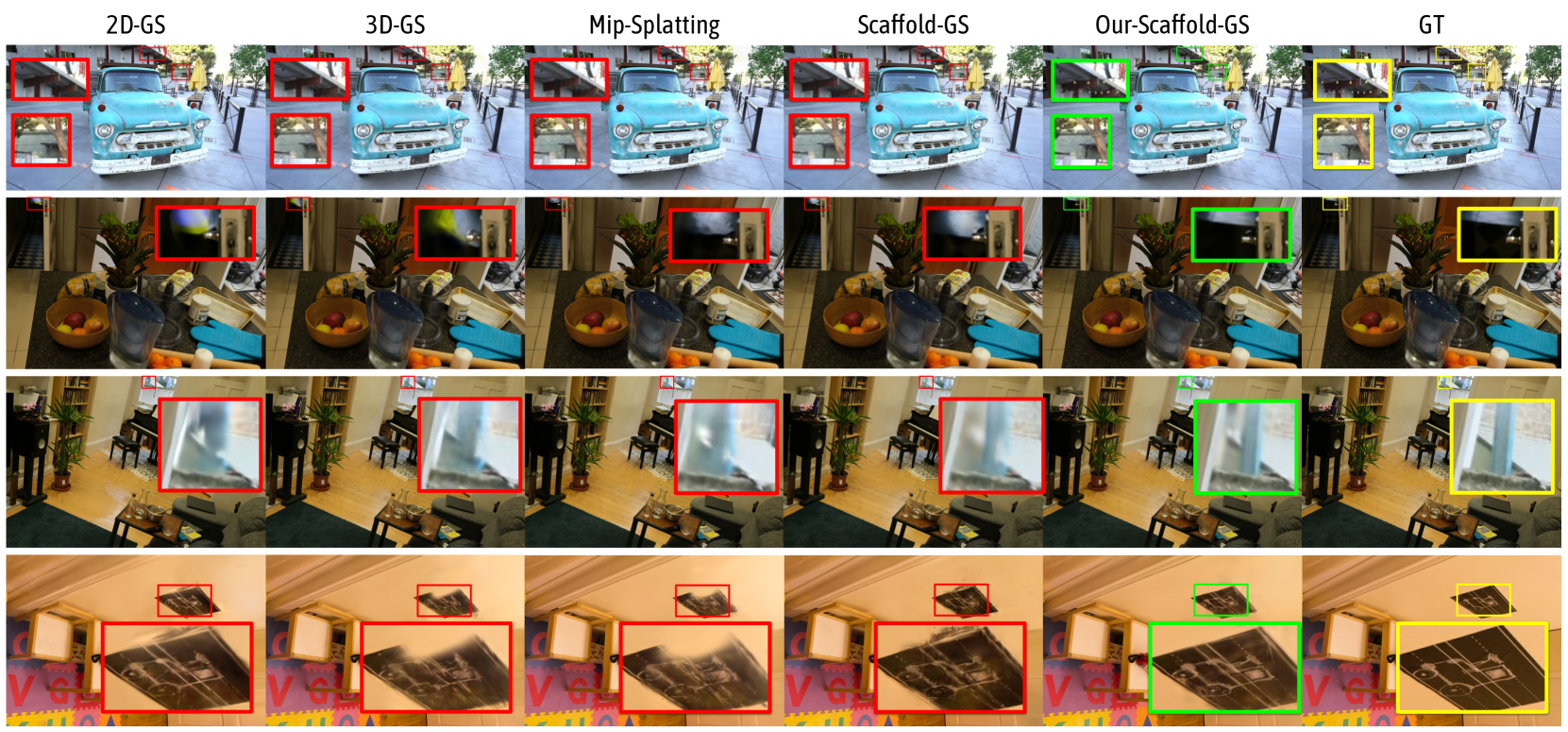
Figure 5: Qualitative comparison of our method and SOTA methods [15, 5, 14, 3] across diverse datasets [50, 60, 61, 51]. We highlight the difference with colored patches. Compared to existing baselines, our method successfully captures very fine details presented in indoor and outdoor scenes, particularly for objects with thin structures such as trees, light-bulbs, decorative texts and etc..
TABLE II: Quantitative comparison on large-scale urban dataset [1, 62, 63]. In addition to three methods compared in Tab. I, we also compare our method with CityGaussian [19] and Hierarchical-GS [2], both of which are specifically targeted at large-scale scenes. It is evident that Octree-GS outperforms the others in both rendering quality and storage efficiency. We highlight best and second-best in each category.
| Dataset Method Metrics 3D-GS [5] | Block_Small PSNR $\uparrow$ 26.82 | Block_All SSIM $\uparrow$ 0.823 | Building LPIPS $\downarrow$ 0.246 | #GS(k)/Mem 1432/3387.4M | PSNR $\uparrow$ 24.45 | SSIM $\uparrow$ 0.746 | LPIPS $\downarrow$ 0.385 | #GS(k)/Mem 979/3584.3M | PSNR $\uparrow$ 22.04 | SSIM $\uparrow$ 0.728 | LPIPS $\downarrow$ 0.332 | #GS(k)/Mem 842/1919.2M |
| --- | --- | --- | --- | --- | --- | --- | --- | --- | --- | --- | --- | --- |
| Mip-Splatting [14] | 27.14 | 0.829 | 0.24 | 860/3654.6M | 24.28 | 0.742 | 0.388 | 694/3061.8M | 22.13 | 0.726 | 0.335 | 1066/2498.6M |
| Scaffold-GS [3] | 29.00 | 0.868 | 0.210 | 357/ 371.2M | 26.30 | 0.808 | 0.293 | 690/ 2272.2M | 22.42 | 0.719 | 0.336 | 438 / 833.2M |
| CityGaussian [19] | 27.46 | 0.808 | 0.267 | 538/4382.7M | 26.26 | 0.800 | 0.324 | 235/4316.6M | 20.94 | 0.706 | 0.310 | 520/3026.8M |
| Hierarchical-GS [2] | 27.69 | 0.823 | 0.276 | 271/1866.7M | 26.00 | 0.803 | 0.306 | 492/4874.2M | 23.28 | 0.769 | 0.273 | 1973/3778.6M |
| Hierarchical-GS( $\tau_{1}$ ) | 27.67 | 0.823 | 0.276 | 271/1866.7M | 25.44 | 0.788 | 0.320 | 435/4874.2M | 23.08 | 0.758 | 0.285 | 1819/3778.6M |
| Hierarchical-GS( $\tau_{2}$ ) | 27.54 | 0.820 | 0.280 | 268/1866.7M | 25.39 | 0.783 | 0.325 | 355/4874.2M | 22.55 | 0.726 | 0.313 | 1473/3778.6M |
| Hierarchical-GS( $\tau_{3}$ ) | 26.60 | 0.794 | 0.319 | 221 /1866.7M | 25.19 | 0.773 | 0.352 | 186 /4874.2M | 21.35 | 0.635 | 0.392 | 820/3778.6M |
| Our-3D-GS | 29.37 | 0.875 | 0.197 | 175 /755.7M | 26.86 | 0.833 | 0.260 | 218 /3205.1M | 22.67 | 0.736 | 0.320 | 447 /1474.5M |
| Our-Scaffold-GS | 29.83 | 0.887 | 0.192 | 360/ 380.3M | 27.31 | 0.849 | 0.229 | 344/ 1648.6M | 23.66 | 0.776 | 0.267 | 619/ 1146.9M |
| Dataset Method Metrics 3D-GS [5] | Rubble PSNR $\uparrow$ 25.20 | Residence SSIM $\uparrow$ 0.757 | Sci-Art LPIPS $\downarrow$ 0.318 | #GS(k)/Mem 956/2355.2M | PSNR $\uparrow$ 21.94 | SSIM $\uparrow$ 0.764 | LPIPS $\downarrow$ 0.279 | #GS(k)/Mem 1209/2498.6M | PSNR $\uparrow$ 21.85 | SSIM $\uparrow$ 0.787 | LPIPS $\downarrow$ 0.311 | #GS(k)/Mem 705/950.6M |
| --- | --- | --- | --- | --- | --- | --- | --- | --- | --- | --- | --- | --- |
| Mip-Splatting [14] | 25.16 | 0.746 | 0.335 | 760/1787.0M | 21.97 | 0.763 | 0.283 | 1301/2570.2M | 21.92 | 0.784 | 0.321 | 615/880.2M |
| Scaffold-GS [3] | 24.83 | 0.721 | 0.353 | 492 / 470.3M | 22.00 | 0.761 | 0.286 | 596/ 697.7M | 22.56 | 0.796 | 0.302 | 526 / 452.5M |
| CityGaussian [19] | 24.67 | 0.758 | 0.286 | 619/3000.3M | 21.92 | 0.774 | 0.257 | 732/3196.0M | 20.07 | 0.757 | 0.290 | 461 /1300.3M |
| Hierarchical-GS [2] | 25.37 | 0.761 | 0.300 | 1541/2345.0M | 21.74 | 0.758 | 0.274 | 2040/2498.6M | 22.02 | 0.810 | 0.257 | 2363/2160.6M |
| Hierarchical-GS( $\tau_{1}$ ) | 25.27 | 0.754 | 0.305 | 1478/2345.0M | 21.70 | 0.756 | 0.276 | 1972/2498.6M | 22.00 | 0.808 | 0.259 | 2226/2160.6M |
| Hierarchical-GS( $\tau_{2}$ ) | 24.80 | 0.724 | 0.329 | 1273/2345.0M | 21.49 | 0.743 | 0.291 | 1694/2498.6M | 21.93 | 0.802 | 0.268 | 1916/2160.6M |
| Hierarchical-GS( $\tau_{3}$ ) | 23.55 | 0.628 | 0.414 | 781/2345.0M | 20.69 | 0.683 | 0.363 | 976/2498.6M | 21.50 | 0.766 | 0.324 | 1165/2160.6M |
| Our-3D-GS | 24.67 | 0.728 | 0.345 | 489 /1392.6M | 21.60 | 0.736 | 0.314 | 350 /986.2M | 22.52 | 0.817 | 0.256 | 630/1331.2M |
| Our-Scaffold-GS | 25.34 | 0.763 | 0.299 | 674/ 693.5M | 22.29 | 0.762 | 0.288 | 344 / 618.8M | 23.38 | 0.828 | 0.240 | 871/ 866.9M |
<details>
<summary>x6.png Details</summary>
### Visual Description
## Image Comparison: 3D-GS vs. Scaffold-GS vs. City-GS vs. Hierarchical-GS vs. Our-Scaffold-GS vs. GT
### Overview
The image presents a visual comparison of different methods for 3D scene reconstruction, specifically "3D-GS", "Scaffold-GS", "City-GS", "Hierarchical-GS", "Our-Scaffold-GS", and "GT" (Ground Truth). The image is divided into three rows, each showing the same scene rendered using the different methods. Red, green, and yellow bounding boxes highlight areas of interest or differences between the methods.
### Components/Axes
* **Titles (Top Row):**
* 3D-GS
* Scaffold-GS
* City-GS
* Hierarchical-GS
* Our-Scaffold-GS
* GT
* **Bounding Boxes:** Red, Green, and Yellow bounding boxes are used to highlight specific regions in each rendering.
### Detailed Analysis
**Row 1: Solar Panel Area**
* **3D-GS:** Contains red bounding boxes around solar panels. The image quality is blurry.
* **Scaffold-GS:** Contains red bounding boxes around solar panels. The image quality is blurry.
* **City-GS:** Contains red bounding boxes around solar panels. The image quality is blurry.
* **Hierarchical-GS:** Contains red bounding boxes around solar panels. The image quality is blurry. Red arrows point to areas of interest.
* **Our-Scaffold-GS:** Contains green bounding boxes around solar panels. The image quality is clearer than the previous methods.
* **GT:** Contains yellow bounding boxes around solar panels. The image quality is the clearest.
**Row 2: Building and Vegetation Area**
* **3D-GS:** Contains red bounding boxes around vegetation near a building.
* **Scaffold-GS:** Contains red bounding boxes around vegetation near a building.
* **City-GS:** Contains red bounding boxes around vegetation near a building.
* **Hierarchical-GS:** Contains red bounding boxes around vegetation near a building. Red arrows point to areas of interest.
* **Our-Scaffold-GS:** Contains green bounding boxes around vegetation near a building.
* **GT:** Contains yellow bounding boxes around vegetation near a building.
**Row 3: Urban Area with Buildings**
* **3D-GS:** Contains red bounding boxes around buildings.
* **Scaffold-GS:** Contains red bounding boxes around buildings.
* **City-GS:** Contains red bounding boxes around buildings.
* **Hierarchical-GS:** Contains red bounding boxes around buildings. Red arrows point to areas of interest.
* **Our-Scaffold-GS:** Contains green bounding boxes around buildings.
* **GT:** Contains yellow bounding boxes around buildings.
### Key Observations
* The "GT" (Ground Truth) images consistently appear to have the highest visual fidelity and clarity.
* "Our-Scaffold-GS" appears to be the next best in terms of visual quality, as indicated by the green bounding boxes.
* "3D-GS", "Scaffold-GS", "City-GS", and "Hierarchical-GS" methods show lower visual quality, with red bounding boxes highlighting areas of interest.
* Red arrows in the "Hierarchical-GS" column indicate specific areas of interest or potential issues.
### Interpretation
The image provides a qualitative comparison of different 3D scene reconstruction methods. The use of bounding boxes (red, green, and yellow) helps to visually assess the accuracy and quality of each method relative to the ground truth. The progression from "3D-GS" to "GT" suggests an improvement in reconstruction quality, with "Our-Scaffold-GS" showing a significant improvement over the other methods, but still falling short of the ground truth. The red arrows in the "Hierarchical-GS" column likely point to artifacts or inaccuracies in the reconstruction. The data suggests that "Our-Scaffold-GS" is a promising approach, but further refinement may be needed to achieve results comparable to the ground truth.
</details>
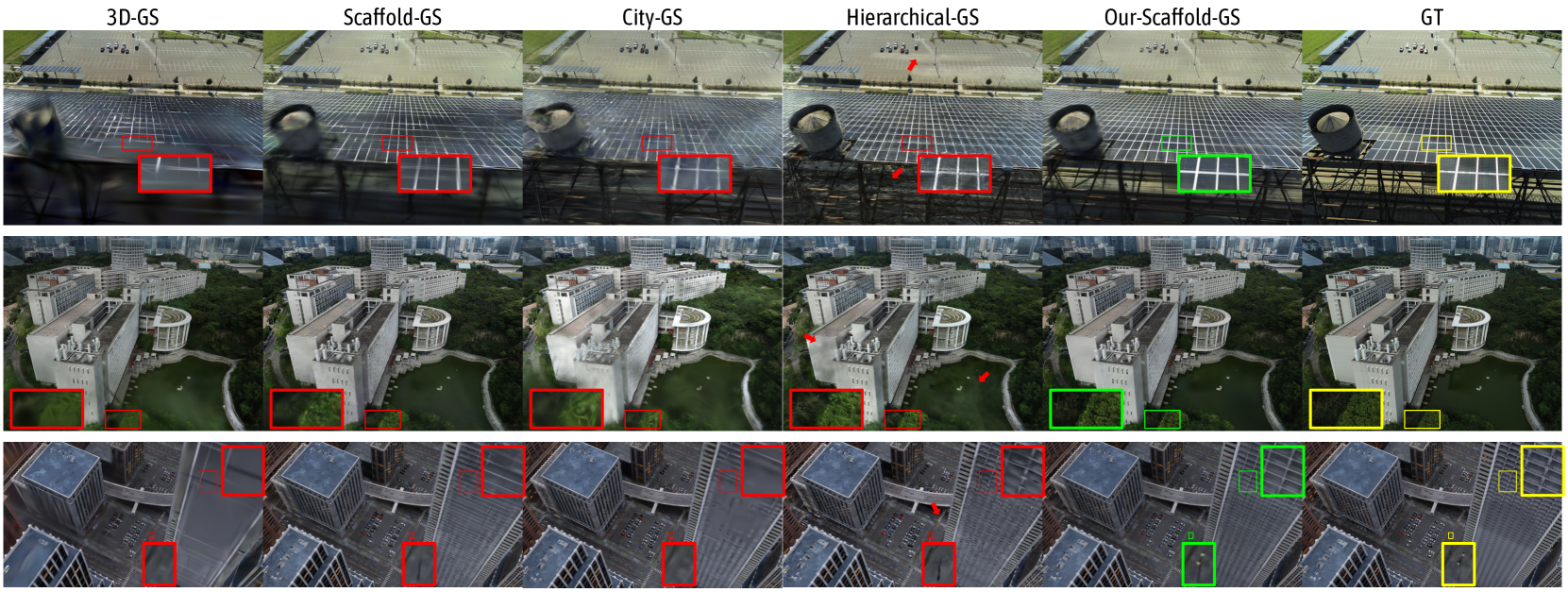
Figure 6: Qualitative comparisons of Octree-GS against baselines [5, 3, 19, 2] across large-scale datasets [62, 63, 1]. As shown in the highlighted patches and arrows above, our method consistently outperforms the baselines, especially in modeling fine details (1st & 3rd row), texture-less regions (2nd row), which are common in large-scale scenes.
V-A Experimental Setup
V-A 1 Datasets
We conduct comprehensive evaluations on $21$ small-scale scenes and $7$ large-scale scenes from various public datasets. Small-scale scenes include 9 scenes from Mip-NeRF360 [50], 2 scenes from Tanks $\&$ Temples [60], 2 scenes in DeepBlending [61] and 8 scenes from BungeeNeRF [51].
For large-scale scenes, we provide a detailed explanation. Specifically, we evaluate on the Block_Small and Block_All scenes (the latter being 10 $×$ larger) in the MatrixCity [1] dataset, which uses Zig-Zag trajectories commonly used in oblique photography. In the MegaNeRF [62] dataset, we choose the Rubble and Building scenes, while in the UrbanScene3D [63] dataset, we select the Residence and Sci-Art scenes. Each scene contains thousands of high-resolution images, and we use COLMAP [54] to obtain sparse SfM points and camera poses. In the Hierarchical-GS [2] dataset, we maintain their original settings and compare both methods on a chunk of the SmallCity scene, which includes 1,470 training images and 30 test images, each paired with depth and mask images.
For the Block_All scene and the SmallCity scene, we employ the train and test information provided by their authors. For other scenes, we uniformly select one out of every eight images as test images, with the remaining images used for training.
V-A 2 Metrics
In addition to the visual quality metrics PSNR, SSIM [64] and LPIPS [65], we also report the file size for storing anchors, the average selected Gaussian primitives used in per-view rendering process, and the rendering speed FPS as a fair indicator for memory and rendering efficiency. We provide the average quantitative metrics on test sets in the main paper and leave the full table for each scene in the supplementary material.
V-A 3 Baselines
We compare our method against 2D-GS [15], 3D-GS [5], Scaffold-GS [3], Mip-Splatting [14] and two concurrent works, CityGaussian [19] and Hierarchical-GS [2]. In the Mip-NeRF360 [50], Tanks $\&$ Temples [60], and DeepBlending [61] datasets, we compare our method with the top four methods. In the large-scale scene datasets MatrixCity [1], MegaNeRF [62] and UrbanScene3D [63], we add the results of CityGaussian and Hierarchical-GS for comparison. To ensure consistency, we remove depth supervision from Hierarchical-GS in these experiments. Following the original setup of Hierarchical-GS, we report results at different granularities (leaves, $\tau_{1}=3$ , $\tau_{2}=6$ , $\tau_{3}=15$ ), each one is after the optimization of the hierarchy. In the street-view dataset, we compare exclusively with Hierarchical-GS, the current state-of-the-art (SOTA) method for street-view data. In this experiment, we apply the same depth supervision used in Hierarchical-GS for fair comparison.
V-A 4 Instances of Our Framework
To demonstrate the generalizability of the proposed framework, we apply it to 2D-GS [15], 3D-GS [5], and Scaffold-GS [3], which we refer to as Our-2D-GS, Our-3D-GS and Our-Scaffold-GS, respectively. In addition, for a fair comparison and deeper analysis, we modify 2D-GS and 3D-GS to anchor versions. Specifically, we voxelize the input SfM points to anchors and assign each of them 2D or 3D Gaussians, while maintaining the same densification strategy as Scaffold-GS. We denote these modified versions as Anchor-2D-GS and Anchor-3D-GS.
V-A 5 Implementation Details
For 3D-GS model we employ standard L1 and SSIM loss, with weights set to 0.8 and 0.2, respectively. For 2D-GS model, we retain the distortion loss $\mathcal{L}_{d}=\sum_{i,j}\omega_{i}\omega_{j}\left|z_{i}-z_{j}\right|$ and normal loss $\mathcal{L}_{n}=\sum_{i}\omega_{i}\left(1-\mathbf{n}_{i}^{\mathrm{T}}\mathbf{N%
}\right)$ , with weights set to 0.01 and 0.05, respectively. For Scaffold-GS model, we keep an additional volume regularization loss $\mathcal{L}_{\mathrm{vol}}=\sum_{i=1}^{N}\operatorname{Prod}\left(s_{i}\right)$ , with a weight set to 0.01.
We adjust the training and densification iterations across all compared methods to ensure a fair comparison. Specifically, for small-scale scenes [50, 60, 61, 51, 2], training was set to 40k iterations, with densification concluding at 20k iterations. For large-scale scenes [1, 62, 63], training was set to 100k iterations, with densification ending at 50k iterations.
We set the voxel size to $0.001$ for all scenes in the modified anchor versions of 2D-GS [15], 3D-GS [5], and Scaffold-GS [3], while for our method, we set the voxel size for the intermediate level of the anchor grid to $0.02$ . For the progress training, we set the total training iteration to $10$ k with $\omega=1.5$ . Since not all layers are fully densified during the progressive training process, we extend the densification by an additional $10$ k iterations, and we set the densification interval $T=100$ empirically. We set the visibility threshold $\tau_{v}$ to $0.7$ for the small-scale scenes [50, 60, 61, 51],as these datasets contain densely captured images, while for large-scale scenes [62, 63, 2], we set $\tau_{v}$ to $0.01$ . In addition, for the multi-scale dataset [51], we set $\tau_{v}$ to $0.2$ .
All experiments are conducted on a single NVIDIA A100 80G GPU. To avoid the impact of image storage on GPU memory, all images were stored on the CPU.
<details>
<summary>x7.png Details</summary>
### Visual Description
## Image Comparison: Text Reconstruction Methods
### Overview
The image presents a visual comparison of different methods for reconstructing text in street-view images. It shows the results of five different approaches: "Hierarchical-GS", "Hierarchical-GS (T2)", "Our-3D-GS", "Our-Scaffold-GS", and "GT" (Ground Truth). Each method is applied to two different scenes, displayed in two rows. The images are annotated with colored bounding boxes highlighting the reconstructed text regions.
### Components/Axes
The image is structured as a grid with two rows and five columns. Each column represents a different text reconstruction method. The rows represent different scenes. The methods are labeled at the top of each column. The bounding boxes are colored red, green, or yellow, depending on the method.
### Detailed Analysis or ### Content Details
**Column 1: Hierarchical-GS**
* **Top Row:** A street scene with a car parked on the side. A red bounding box highlights the reconstructed text on the car's license plate area. A small red arrow points to a spot on the road. A small red bounding box highlights the text on a sign on the building.
* Text in red box on car: "DANS"
* **Bottom Row:** A building facade with a scooter parked in front. Red bounding boxes highlight the reconstructed text on the building's architectural details and a sign.
**Column 2: Hierarchical-GS (T2)**
* **Top Row:** Similar street scene as in Column 1. A red bounding box highlights the reconstructed text on the car's license plate area. A small red bounding box highlights the text on a sign on the building.
* **Bottom Row:** Similar building facade as in Column 1. Red bounding boxes highlight the reconstructed text on the building's architectural details and a sign.
**Column 3: Our-3D-GS**
* **Top Row:** Similar street scene as in Column 1. A red bounding box highlights the reconstructed text on the car's license plate area. A small red bounding box highlights the text on a sign on the building.
* Text in red box on car: "ENAGE DANS"
* **Bottom Row:** Similar building facade as in Column 1. Red bounding boxes highlight the reconstructed text on the building's architectural details and a sign.
**Column 4: Our-Scaffold-GS**
* **Top Row:** Similar street scene as in Column 1. A green bounding box highlights the reconstructed text on the car's license plate area.
* Text in green box on car: "BRAYA FINAGE DANS"
* **Bottom Row:** Similar building facade as in Column 1. Green bounding boxes highlight the reconstructed text on the building's architectural details and a sign.
**Column 5: GT (Ground Truth)**
* **Top Row:** Similar street scene as in Column 1. A yellow bounding box highlights the reconstructed text on the car's license plate area. A yellow bounding box highlights the text on a sign on the building.
* Text in yellow box on car: "BRAYA EINAGE DANS"
* **Bottom Row:** Similar building facade as in Column 1. Yellow bounding boxes highlight the reconstructed text on the building's architectural details and a sign.
### Key Observations
* The "GT" column represents the ground truth, showing the ideal text reconstruction.
* The different methods show varying degrees of success in reconstructing the text.
* "Our-Scaffold-GS" appears to produce results closer to the ground truth compared to "Hierarchical-GS" and "Our-3D-GS".
* The red arrow in the first image of "Hierarchical-GS" does not appear to be related to text reconstruction.
### Interpretation
The image provides a visual comparison of different text reconstruction methods in street-view images. The goal is to assess the accuracy and effectiveness of each method in recovering text from real-world scenes. The "GT" column serves as a benchmark for evaluating the performance of the other methods. The results suggest that "Our-Scaffold-GS" performs better than "Hierarchical-GS" and "Our-3D-GS" in the specific scenes depicted. The differences in performance likely stem from the underlying algorithms and assumptions of each method. The image highlights the challenges of text reconstruction in complex environments and the importance of developing robust and accurate algorithms.
</details>
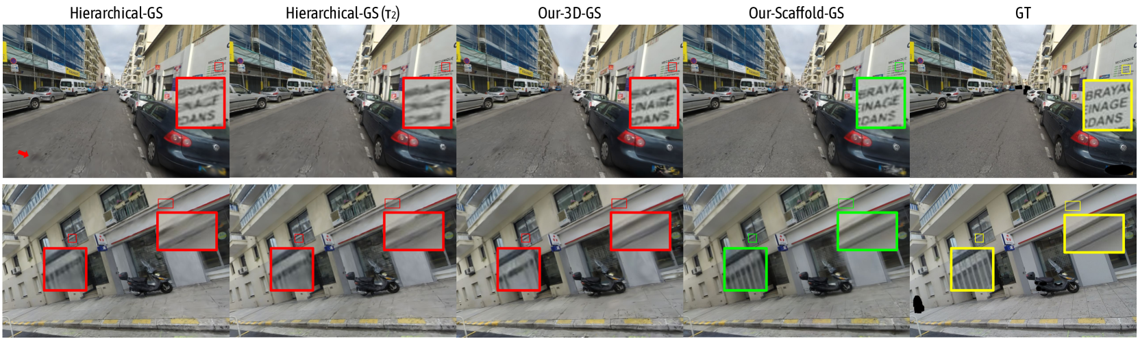
Figure 7: Qualitative comparisons of our approach against Hierarchical-GS [2]. We present both the highest-quality setting (leaves) and a reasonably reduced LOD setting ( $\tau_{2}$ = 6 pixels). Octree-GS demonstrates superior performance in street views, specially in thin geometries and texture-less regions (e.g., railings, signs and pavements.)
TABLE III: Quantitative comparison on the SMALLCITY scene of the Hierarchical-GS [2] dataset. The competing metrics are sourced from the original paper.
| Method | PSNR( $\uparrow$ ) | SSIM( $\uparrow$ ) | LPIPS( $\downarrow$ ) | FPS( $\uparrow$ ) |
| --- | --- | --- | --- | --- |
| 3D-GS [5] | 25.34 | 0.776 | 0.337 | 99 |
| Hierarchical-GS [2] | 26.62 | 0.820 | 0.259 | 58 |
| Hierarchical-GS( $\tau_{1}$ ) | 26.53 | 0.817 | 0.263 | 86 |
| Hierarchical-GS( $\tau_{2}$ ) | 26.29 | 0.810 | 0.275 | 110 |
| Hierarchical-GS( $\tau_{3}$ ) | 25.68 | 0.786 | 0.324 | 159 |
| Our-3D-GS | 25.77 | 0.811 | 0.272 | 130 |
| Our-Scaffold-GS | 26.10 | 0.826 | 0.235 | 89 |
<details>
<summary>x8.png Details</summary>
### Visual Description
## Image Comparison: 2D-GS Methods
### Overview
The image presents a side-by-side comparison of three different 2D-GS (Gaussian Splatting) methods applied to the same scene. The scene appears to be a forest floor with a tree stump. Each method's result is displayed with a title indicating the method used, a dB (decibel) value, a K value, and an M value. The images are annotated with rectangular regions highlighting specific areas, with red rectangles for the first two methods and green rectangles for the third.
### Components/Axes
* **Titles:**
* (a) 2D-GS: 26.16dB/413K/670M
* (b) Anchor-2D-GS: 26.25dB/491K/359M
* (c) Our-2D-GS: 26.40dB/385K/293M
* **Annotations:** Red and green rectangles highlighting regions in each image.
### Detailed Analysis or Content Details
* **(a) 2D-GS:**
* Title: 2D-GS: 26.16dB/413K/670M
* Two red rectangles are present in the upper portion of the image, highlighting areas of the background.
* Two red rectangles are present near the base of the tree stump, highlighting details.
* **(b) Anchor-2D-GS:**
* Title: Anchor-2D-GS: 26.25dB/491K/359M
* Two red rectangles are present in the upper portion of the image, highlighting areas of the background.
* Two red rectangles are present near the base of the tree stump, highlighting details.
* **(c) Our-2D-GS:**
* Title: Our-2D-GS: 26.40dB/385K/293M
* Two green rectangles are present in the upper portion of the image, highlighting areas of the background.
* Two green rectangles are present near the base of the tree stump, highlighting details.
### Key Observations
* The dB values increase from (a) to (c): 26.16dB, 26.25dB, 26.40dB.
* The K values decrease from (a) to (c): 413K, 491K, 385K.
* The M values decrease significantly from (a) to (c): 670M, 359M, 293M.
* The highlighted regions appear to focus on areas where the differences between the methods are most apparent.
### Interpretation
The image compares the performance of three 2D Gaussian Splatting methods. The dB values likely represent a measure of quality or signal-to-noise ratio, with higher values indicating better performance. The K and M values likely represent the size or complexity of the model, with lower values indicating a more efficient model.
The data suggests that "Our-2D-GS" (c) achieves the highest dB value (26.40dB) while also having the lowest M value (293M), indicating a potentially superior method in terms of both quality and efficiency. The highlighted regions likely draw attention to areas where the visual differences between the methods are most noticeable, possibly in terms of detail, clarity, or artifact reduction.
</details>
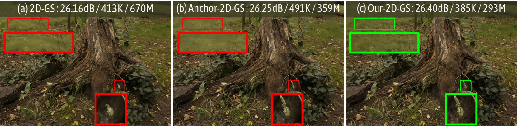
Figure 8: Comparison of different versions of the 2D-GS [15] model. We showcase the rendering results on the stump scene from the Mip-NeRF360 [50] dataset. We report PSNR, average number of Gaussians for rendering and storage size.
TABLE IV: Quantitative comparison on the BungeeNeRF [51] dataset. We provide metrics for each scale and their average across all four. Scale-1 denotes the closest views, while scale-4 covers the entire landscape. We note a notable rise in Gaussian counts for baseline methods when zooming out from scale 1 to 4, whereas our method maintains a significantly lower count, ensuring consistent rendering speed across all LOD levels. We highlight best and second-best in each category.
| Dataset | BungeeNeRF (Average) | scale-1 | scale-2 | scale-3 | scale-4 | | | | | | | |
| --- | --- | --- | --- | --- | --- | --- | --- | --- | --- | --- | --- | --- |
| Method Metrics | PSNR $\uparrow$ | SSIM $\uparrow$ | LPIPS $\downarrow$ | #GS(k)/Mem | PSNR $\uparrow$ | #GS(k) | PSNR $\uparrow$ | #GS(k) | PSNR $\uparrow$ | #GS(k) | PSNR $\uparrow$ | #GS(k) |
| 2D-GS [5] | 27.10 | 0.903 | 0.121 | 1079/886.1M | 28.18 | 205 | 28.11 | 494 | 25.99 | 1826 | 23.71 | 2365 |
| 3D-GS [5] | 27.79 | 0.917 | 0.093 | 2686/1792.3M | 30.00 | 522 | 28.97 | 1272 | 26.19 | 4407 | 24.20 | 5821 |
| Mip-Splatting [14] | 28.14 | 0.918 | 0.094 | 2502/1610.2M | 29.79 | 503 | 29.37 | 1231 | 26.74 | 4075 | 24.44 | 5298 |
| Scaffold-GS [3] | 28.16 | 0.917 | 0.095 | 1652/ 319.2M | 30.48 | 303 | 29.18 | 768 | 26.56 | 2708 | 24.95 | 3876 |
| Anchor-2D-GS | 27.18 | 0.885 | 0.140 | 1050/533.8M | 29.80 | 260 | 28.26 | 601 | 25.43 | 1645 | 23.71 | 2026 |
| Anchor-3D-GS | 27.90 | 0.909 | 0.114 | 1565/790.3M | 30.85 | 391 | 29.29 | 905 | 26.13 | 2443 | 24.49 | 3009 |
| Our-2D-GS | 27.34 | 0.893 | 0.129 | 676 /736.1M | 30.09 | 249 | 28.72 | 511 | 25.42 | 1003 | 23.41 | 775 |
| Our-3D-GS | 27.94 | 0.909 | 0.110 | 952 /1045.7M | 31.11 | 411 | 29.42 | 819 | 25.88 | 1275 | 23.77 | 938 |
| Our-Scaffold-GS | 28.39 | 0.923 | 0.088 | 1474/ 296.7M | 31.11 | 486 | 29.59 | 1010 | 26.51 | 2206 | 25.07 | 2167 |
V-B Results Analysis
Our evaluation encompasses a wide range of scenes, including indoor and outdoor environments, both synthetic and real-world, as well as large-scale urban scenes from both aerial views and street views. We demonstrate that our method preserves fine-scale details while reducing the number of Gaussians, resulting in faster rendering speed and lower storage overhead, as shown in Fig. 5, 6, 7, 8 and Tab. I, IV, II, III, V.
V-B 1 Performance Analysis
Quality Comparisons
Our method introduces anchors with octree structure, which decouple multi-scale Gaussian primitives into varying LOD levels. This approach enables finer Gaussian primitives to capture scene details more accurately, thereby enhancing the overall rendering quality. In Fig. 5, 6, 7 and Tab. I, II, III, we compare Octree-GS to previous state-of-the-art (SOTA) methods, demonstrating that our method consistently outperforms the baselines across both small-scale and large-scale scenes, especially in fine details and texture-less regions. Notably, when compared to Hierarchical-GS [2] on the street-view dataset, Octree-GS exhibits slightly lower PSNR values but significantly better visual quality, with LPIPS scores of 0.235 for ours and 0.259 for theirs.
Storage Comparisons
As shown in Tab. I, II, our method reduces the number of Gaussian primitives used for rendering, resulting in faster rendering speed and lower storage overhead. This demonstrates the benefits of our two main improvements: 1) our LOD structure efficiently arranges Gaussian primitives, with coarse primitives representing low-frequency scene information, which previously required redundant primitives; and 2) our view-frequency strategy significantly prunes unnecessary primitives.
Variants Comparisons
As described in Sec. IV, our method is agnostic to the specific Gaussian representation and can be easily adapted to any Gaussian-based method with minimal effort. In Tab. I, the modified anchor-version of 2D-GS [15] and 3D-GS [5] achieve competitive rendering quality with fewer file storage than the original methods. This demonstrates that the anchor design organizes the Gaussian primitives more efficiently, reducing redundancy and creating a more compact way. More than the anchor design, Octree-GS delivers better visual performance and fewer Gaussian primitives as shown in Tab. I, which benefits from the explicit, multi-level anchor design. In Fig. 8, we compare the vanilla 2D-GS with the anchor-version and octree-version method. Among them, the octree-version provides the most detail and the least amount of Gaussian primitives and storage.
TABLE V: Quantitative comparison of rendering speed on the MatrixCity [1] dataset. We report the averaged FPS on three novel view trajectories (Fig. 9). Our method shows consistent rendering speed above $30$ FPS at $2k$ image resolution while all baseline methods fail to meet the real-time performance.
| Method Traj. 3D-GS [5] Scaffold-GS [3] | $T_{1}$ 13.81 6.69 | $T_{2}$ 11.70 7.37 | $T_{3}$ 13.50 8.04 |
| --- | --- | --- | --- |
| Hierarchical-GS [2] | 9.13 | 8.54 | 8.91 |
| Hierarchical-GS( $\tau_{1}$ ) | 16.14 | 13.26 | 14.79 |
| Hierarchical-GS( $\tau_{2}$ ) | 19.70 | 19.59 | 18.94 |
| Hierarchical-GS( $\tau_{3}$ ) | 24.33 | 25.29 | 24.75 |
| Our-3D-GS | 57.08 | 56.85 | 56.07 |
| Our-Scaffold-GS | 40.91 | 35.17 | 40.31 |
<details>
<summary>x9.png Details</summary>
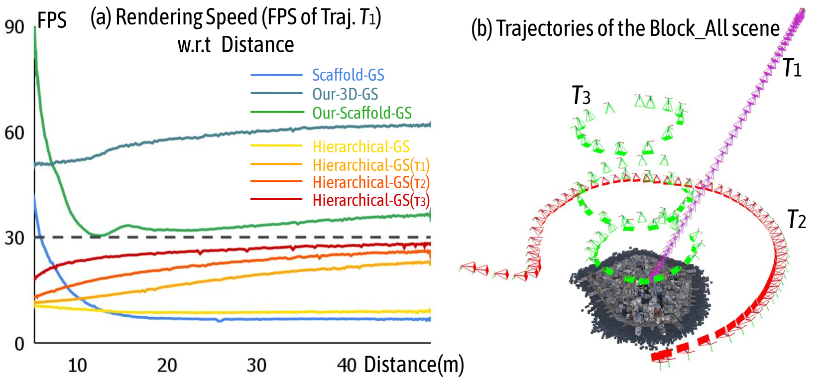
### Visual Description
## Chart and Diagram: Rendering Speed vs. Distance and Trajectories
### Overview
The image presents two sub-figures: (a) a line chart comparing the rendering speed (FPS) of different methods with respect to distance for trajectory T1, and (b) a diagram illustrating the trajectories of the Block_All scene.
### Components/Axes
**Sub-figure (a): Rendering Speed vs. Distance**
* **Title:** Rendering Speed (FPS of Traj. T1) w.r.t Distance
* **X-axis:** Distance (m), with markers at 10, 20, 30, and 40.
* **Y-axis:** FPS, with markers at 0, 30, 60, and 90.
* **Legend (Top-Right):**
* Blue: Scaffold-GS
* Dark Blue: Our-3D-GS
* Green: Our-Scaffold-GS
* Yellow: Hierarchical-GS
* Orange: Hierarchical-GS(T1)
* Red-Orange: Hierarchical-GS(T2)
* Red: Hierarchical-GS(T3)
* **Horizontal Line:** A dashed gray line is present at FPS = 30.
**Sub-figure (b): Trajectories of the Block_All scene**
* **Title:** Trajectories of the Block_All scene
* **Trajectories:** Three trajectories are shown, labeled T1, T2, and T3.
* T1: Purple
* T2: Red
* T3: Green
* **Scene Representation:** A cluster of dark gray points represents the "Block_All" scene.
* **Camera Icons:** Small camera icons are placed along each trajectory, indicating camera positions.
### Detailed Analysis
**Sub-figure (a): Rendering Speed vs. Distance**
* **Scaffold-GS (Blue):** Starts at approximately 30 FPS at a distance of 0m, decreases to approximately 5 FPS by 10m, and remains relatively constant at around 5 FPS from 10m to 40m.
* **Our-3D-GS (Dark Blue):** Starts at approximately 50 FPS at a distance of 0m, increases to approximately 60 FPS by 20m, and remains relatively constant at around 60 FPS from 20m to 40m.
* **Our-Scaffold-GS (Green):** Starts at approximately 90 FPS at a distance of 0m, decreases sharply to approximately 30 FPS by 10m, then increases slightly to approximately 35 FPS by 20m, and remains relatively constant at around 35 FPS from 20m to 40m.
* **Hierarchical-GS (Yellow):** Starts at approximately 15 FPS at a distance of 0m, decreases slightly to approximately 10 FPS by 10m, and remains relatively constant at around 10 FPS from 10m to 40m.
* **Hierarchical-GS(T1) (Orange):** Starts at approximately 15 FPS at a distance of 0m, increases to approximately 25 FPS by 40m.
* **Hierarchical-GS(T2) (Red-Orange):** Starts at approximately 20 FPS at a distance of 0m, increases to approximately 28 FPS by 40m.
* **Hierarchical-GS(T3) (Red):** Starts at approximately 25 FPS at a distance of 0m, increases to approximately 28 FPS by 40m.
**Sub-figure (b): Trajectories of the Block_All scene**
* **T1 (Purple):** A straight trajectory moving away from the scene.
* **T2 (Red):** A curved trajectory that loops around the scene.
* **T3 (Green):** A complex trajectory with multiple loops around the scene.
### Key Observations
* Our-3D-GS consistently maintains a high FPS compared to other methods across all distances.
* Scaffold-GS and Hierarchical-GS have the lowest FPS.
* The Hierarchical-GS variants (T1, T2, T3) show a gradual increase in FPS with distance.
* The trajectories in sub-figure (b) provide a visual representation of the camera movement around the Block_All scene.
### Interpretation
The data suggests that Our-3D-GS is the most efficient rendering method for the given scene and trajectory (T1), maintaining a consistently high frame rate as distance increases. Scaffold-GS and Hierarchical-GS are less efficient, with significantly lower frame rates. The trajectories in sub-figure (b) illustrate different camera paths around the scene, which may influence the rendering performance of the various methods. The horizontal line at 30 FPS likely represents a target or minimum acceptable frame rate for real-time rendering. The Hierarchical-GS variants show a slight improvement in FPS as distance increases, potentially due to optimizations related to level-of-detail or scene simplification at greater distances.
</details>
Figure 9: (a) The figure shows the rendering speed with respect to distance for different methods along trajectory $T_{1}$ , both Our-3D-GS and Our-Scaffold-GS achieve real-time rendering speeds ( $≥ 30$ FPS). (b) The visualization depicts three different trajectories, corresponding to $T_{1}$ , $T_{2}$ , and $T_{3}$ in Tab. V, which are commonly found in video captures of large-scale scenes and illustrate the practical challenges involved.
V-B 2 Efficiency Analysis
Rendering Time Comparisons
Our goal is to enable real-time rendering of Gaussian representation models at any position within the scene using Level-of-Detail techniques. To evaluate our approach, we compare Octree-GS with three state-of-the-art methods [5, 3, 2] on three novel view trajectories in Tab. V and Fig. 9. These trajectories represent common movements in large-scale scenes, such as zoom-in, 360-degree circling, and multi-scale circling. As shown in Tab. V and Fig. 5, our method excels at capturing fine-grained details in close views while maintaining consistent rendering speeds at larger scales. Notably, our rendering speed is nearly $10×$ faster than Scaffold-GS [3] in large-scale scenes and extreme-view sequences, which depends on our innovative LOD structure design.
Training Time Comparisons
While our core contribution is the acceleration of rendering speed through LOD design, training speed is also critical for the practical application of photorealistic scene reconstruction. Below, we provide statistics for the Mip-NeRF360 [50] dataset (40k iterations): 2D-GS (28 mins), 3D-GS (34 mins), Mip-Splatting (46 mins), Scaffold-GS (29 mins), and Our-2D-GS (20 mins), Our-3D-GS (21 mins), Our-Scaffold-GS (23 mins). Additionally, we report the training time for the concurrent work, Hierarchical-GS [2]. This method requires three stages to construct the LOD structure, which result in a longer training time (38 minutes for the first stage, totaling 69 minutes). In contrast, under the same number of iterations, our proposed method requires less time. Our-Scaffold-GS achieves the construction and optimization of the LOD structure in a single stage, taking only 35 minutes. The reason our method can accelerate training time is twofold: the number of Gaussian primitives is relatively smaller, and not all Gaussians need to be optimized during progressive training.
TABLE VI: Quantitative comparison on multi-resolution Mip-NeRF360 [50] dataset. Octree-GS achieves better rendering quality across all scales compared to baselines.
| 3D-GS [5] | 26.16 | 0.757 | 0.301 | 27.33 | 0.822 | 0.202 | 28.55 | 0.884 | 0.117 | 27.85 | 0.897 | 0.086 | 430 |
| --- | --- | --- | --- | --- | --- | --- | --- | --- | --- | --- | --- | --- | --- |
| Scaffold-GS [3] | 26.81 | 0.767 | 0.285 | 28.09 | 0.835 | 0.183 | 29.52 | 0.898 | 0.099 | 28.98 | 0.915 | 0.072 | 369 |
| Mip-Splatting [14] | 27.43 | 0.801 | 0.244 | 28.56 | 0.857 | 0.152 | 30.00 | 0.910 | 0.087 | 31.05 | 0.942 | 0.055 | 642 |
| Our-Scaffold-GS | 27.68 | 0.791 | 0.245 | 28.82 | 0.850 | 0.157 | 30.27 | 0.906 | 0.087 | 31.18 | 0.932 | 0.057 | 471 |
<details>
<summary>x10.png Details</summary>
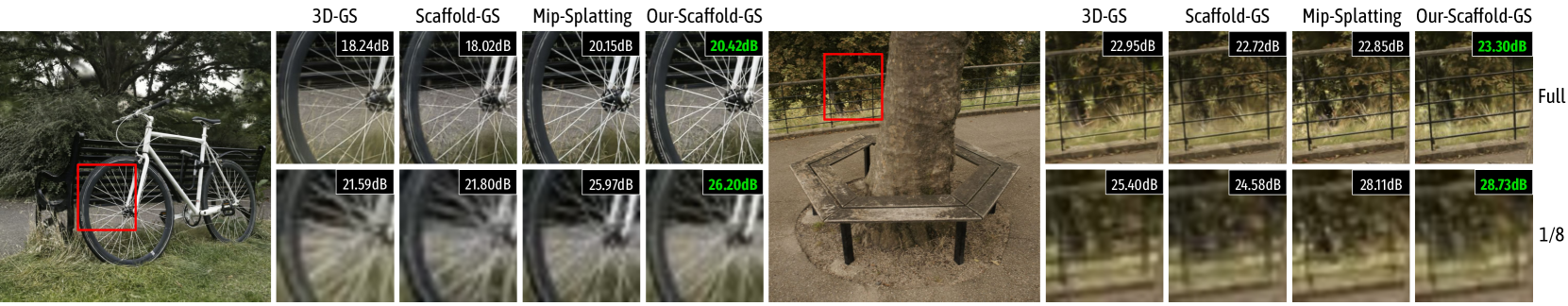
### Visual Description
## Image Comparison: 3D-GS vs. Scaffold-GS vs. Mip-Splatting vs. Our-Scaffold-GS
### Overview
The image presents a visual comparison of four rendering techniques: 3D-GS, Scaffold-GS, Mip-Splatting, and Our-Scaffold-GS. Two different scenes are shown: a bicycle in a park setting and a tree with a bench. For each scene, the image quality of each rendering technique is compared at two resolutions: "Full" and "1/8". The image quality is quantified using a "dB" metric, with higher values indicating better quality. Red rectangles highlight specific regions of interest in the original images.
### Components/Axes
* **Rendering Techniques (Horizontal Axis):** 3D-GS, Scaffold-GS, Mip-Splatting, Our-Scaffold-GS
* **Scenes:** Bicycle, Tree with Bench
* **Resolutions (Vertical Axis):** Full, 1/8
* **Metric:** dB (Decibels, presumably a measure of image quality)
### Detailed Analysis
**Scene 1: Bicycle**
* **Full Resolution:**
* 3D-GS: 18.24dB
* Scaffold-GS: 18.02dB
* Mip-Splatting: 20.15dB
* Our-Scaffold-GS: 20.42dB (Green text)
* **1/8 Resolution:**
* 3D-GS: 21.59dB
* Scaffold-GS: 21.80dB
* Mip-Splatting: 25.97dB
* Our-Scaffold-GS: 26.20dB (Green text)
**Scene 2: Tree with Bench**
* **Full Resolution:**
* 3D-GS: 22.95dB
* Scaffold-GS: 22.72dB
* Mip-Splatting: 22.85dB
* Our-Scaffold-GS: 23.30dB (Green text)
* **1/8 Resolution:**
* 3D-GS: 25.40dB
* Scaffold-GS: 24.58dB
* Mip-Splatting: 28.11dB
* Our-Scaffold-GS: 28.73dB (Green text)
### Key Observations
* In all cases, "Our-Scaffold-GS" achieves the highest dB value, indicated by the green text.
* Image quality (dB) generally increases when moving from "Full" to "1/8" resolution, suggesting that the rendering techniques perform better at lower resolutions, or that the metric is more favorable at lower resolutions.
* The difference in dB values between the techniques is more pronounced in the "1/8" resolution images.
### Interpretation
The image provides evidence that "Our-Scaffold-GS" rendering technique consistently outperforms the other three techniques (3D-GS, Scaffold-GS, and Mip-Splatting) in terms of the dB metric used to assess image quality. This advantage is observed across two different scenes and at both full and 1/8 resolutions. The green text highlights the superior performance of "Our-Scaffold-GS". The increase in dB values at 1/8 resolution suggests that these rendering techniques may be more effective or optimized for lower resolution images, or that the dB metric is more sensitive to differences in lower resolution images. The red rectangles highlight areas of interest for visual comparison, but the dB values provide a quantitative measure of the differences.
</details>
Figure 10: Qualitative comparison of full-resolution and low-resolution (1/8 of full-resolution) on multi-resolution Mip-NeRF360 [50] datasets. Our approach demonstrates adaptive anti-aliasing and effectively recovers fine-grained details, while baselines often produce artifacts, particularly on elongated structures such as bicycle wheels and handrails.
V-B 3 Robustness Analysis
<details>
<summary>x11.png Details</summary>
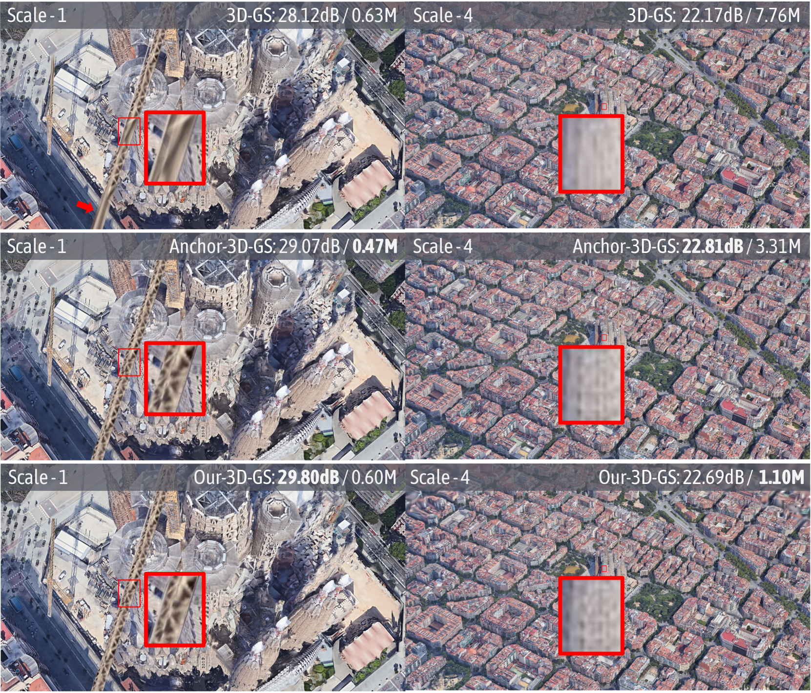
### Visual Description
## Image Comparison: 3D-GS vs. Anchor-3D-GS vs. Our-3D-GS
### Overview
The image presents a visual comparison of three different methods (3D-GS, Anchor-3D-GS, and Our-3D-GS) for rendering a 3D scene at two different scales (Scale-1 and Scale-4). Each method is evaluated based on two metrics: a dB value (likely a signal-to-noise ratio or similar quality metric) and a value in "M" (likely representing memory usage in Megabytes). The scene appears to be an aerial view of a city, with a detailed view of a building (likely Sagrada Familia) at Scale-1 and a broader view of the city at Scale-4. Red boxes highlight specific areas for closer inspection.
### Components/Axes
* **Rows:** Each row represents a different method:
* Row 1: 3D-GS
* Row 2: Anchor-3D-GS
* Row 3: Our-3D-GS
* **Columns:** Each column represents a different scale:
* Column 1: Scale-1 (detailed view of a building)
* Column 2: Scale-4 (broader view of the city)
* **Metrics:** Each image is labeled with two metrics:
* dB value (e.g., 28.12dB) - likely a measure of image quality or signal-to-noise ratio.
* Value in "M" (e.g., 0.63M) - likely memory usage in Megabytes.
* **Red Boxes:** Each image contains one or two red boxes highlighting a specific region for closer inspection.
### Detailed Analysis or ### Content Details
**Row 1: 3D-GS**
* **Scale-1:**
* Label: "Scale -1" (top-left)
* Metric: "3D-GS: 28.12dB / 0.63M" (top-right)
* Image: Detailed view of a building (Sagrada Familia). A red arrow points to a specific area. A small red box highlights a region, and a larger red box zooms in on that region.
* **Scale-4:**
* Label: "Scale - 4" (top-left)
* Metric: "3D-GS: 22.17dB / 7.76M" (top-right)
* Image: Broader aerial view of a city. A red box highlights a region.
**Row 2: Anchor-3D-GS**
* **Scale-1:**
* Label: "Scale -1" (top-left)
* Metric: "Anchor-3D-GS: 29.07dB / 0.47M" (top-right)
* Image: Detailed view of a building (Sagrada Familia). A small red box highlights a region, and a larger red box zooms in on that region.
* **Scale-4:**
* Label: "Scale - 4" (top-left)
* Metric: "Anchor-3D-GS: 22.81dB / 3.31M" (top-right)
* Image: Broader aerial view of a city. A red box highlights a region.
**Row 3: Our-3D-GS**
* **Scale-1:**
* Label: "Scale -1" (top-left)
* Metric: "Our-3D-GS: 29.80dB / 0.60M" (top-right)
* Image: Detailed view of a building (Sagrada Familia). A small red box highlights a region, and a larger red box zooms in on that region.
* **Scale-4:**
* Label: "Scale - 4" (top-left)
* Metric: "Our-3D-GS: 22.69dB / 1.10M" (top-right)
* Image: Broader aerial view of a city. A red box highlights a region.
### Key Observations
* **dB Values:** At Scale-1, "Our-3D-GS" has the highest dB value (29.80dB), followed by "Anchor-3D-GS" (29.07dB) and then "3D-GS" (28.12dB). At Scale-4, "Anchor-3D-GS" has the highest dB value (22.81dB), followed by "Our-3D-GS" (22.69dB) and then "3D-GS" (22.17dB).
* **Memory Usage:** At Scale-1, "Anchor-3D-GS" has the lowest memory usage (0.47M), followed by "Our-3D-GS" (0.60M) and then "3D-GS" (0.63M). At Scale-4, "Our-3D-GS" has the lowest memory usage (1.10M), followed by "Anchor-3D-GS" (3.31M) and then "3D-GS" (7.76M).
* **Visual Detail:** The red boxes highlight areas where the visual differences between the methods are likely most apparent.
### Interpretation
The image presents a performance comparison of three different 3D rendering techniques. The dB values suggest the quality of the rendering, with higher values indicating better quality. The "M" values indicate the memory footprint of each method.
At Scale-1 (detailed view), "Our-3D-GS" appears to offer the best quality (highest dB) with a memory footprint comparable to "3D-GS". "Anchor-3D-GS" has the lowest memory usage but a slightly lower dB value.
At Scale-4 (broader view), "Anchor-3D-GS" has the highest dB value, while "Our-3D-GS" has the lowest memory usage. "3D-GS" has the lowest dB value and the highest memory usage.
The choice of which method is "best" depends on the specific application and the trade-off between quality and memory usage. If memory is a primary constraint, "Our-3D-GS" might be preferred at Scale-4. If quality is paramount, "Our-3D-GS" might be preferred at Scale-1, and "Anchor-3D-GS" at Scale-4. The red boxes are intended to allow visual inspection of the rendering quality in specific areas of the scene.
</details>
Figure 11: Qualitative comparison of scale-1 and scale-4 on the Barcelona scene from the BungeeNeRF [51] dataset. Both Anchor-3D-GS and Our-3D-GS accurately reconstruct fine details, such as the crane in scale-1 and the building surface in scale-4 (see highlighted patches and arrows), while Our-3D-GS uses fewer primitives to model the entire scene. We report PSNR and the number of Gaussians used for rendering.
Multi-Scale Results
To evaluate the ability of Octree-GS to handle multi-scale scene details, we conduct an experiment using the BungeeNeRF [51] dataset across four different scales (i.e., from ground-level to satellite-level camera altitudes). Our results show that Octree-GS accurately captures scene details and models the entire scene more efficiently with fewer Gaussian primitives, as demonstrated in Tab. IV and Fig. 11.
Multi-Resolution Results
As mentioned in Sec. IV, when dealing with training views that vary in camera resolution or intrinsics, such as datasets presented in [50] with a four-fold downsampling operation, we multiply the observation distance with factor scale factor accordingly to handle this multi-resolution dataset. As shown in Fig. 10 and Tab. VI, we train all models on images with downsampling scales of 1, 2, 4, 8, and Octree-GS adaptively handle the changed footprint size and effectively address the aliasing issues inherent to 3D-GS [5] and Scaffold-GS [3]. As resolution changes, 3D-GS and Scaffold-GS introduce noticeable erosion artifacts, but our approach avoids such issues, achieving results competitive with Mip-Splatting [14] and even closer to the ground truth. Additionally, we provide multi-resolution results for the Tanks&Temples dataset [60] and the Deep Blending dataset [61] in the supplementary materials.
Random Initialization Results
To illustrate the independence of our framework from SfM points, we evaluate it using randomly initialized points, with 0.31/0.27 (LPIPS $\downarrow$ ), 25.93/26.41 (PSNR $\uparrow$ ), 0.76/0.77 (SSIM $\uparrow$ ) on Mip-NeRF360 [50] dataset comparing Scaffold-GS with Our-Scaffold-GS. The improvement primarily depends on the efficient densification strategy.
Appearance Embedding Results
We demonstrate that our specialized design can handle input images with different exposure compensations and provide detailed control over lighting and appearance. As shown in Fig. 12, we reconstruct two scenes: one is from the widely-used Phototourism [66] dataset and the other is a self-captured scene of a ginkgo tree. We present five images rendered from a fixed camera view, where we interpolate the appearance codes linearly to produce a fancy style transfer effect.
<details>
<summary>x12.png Details</summary>
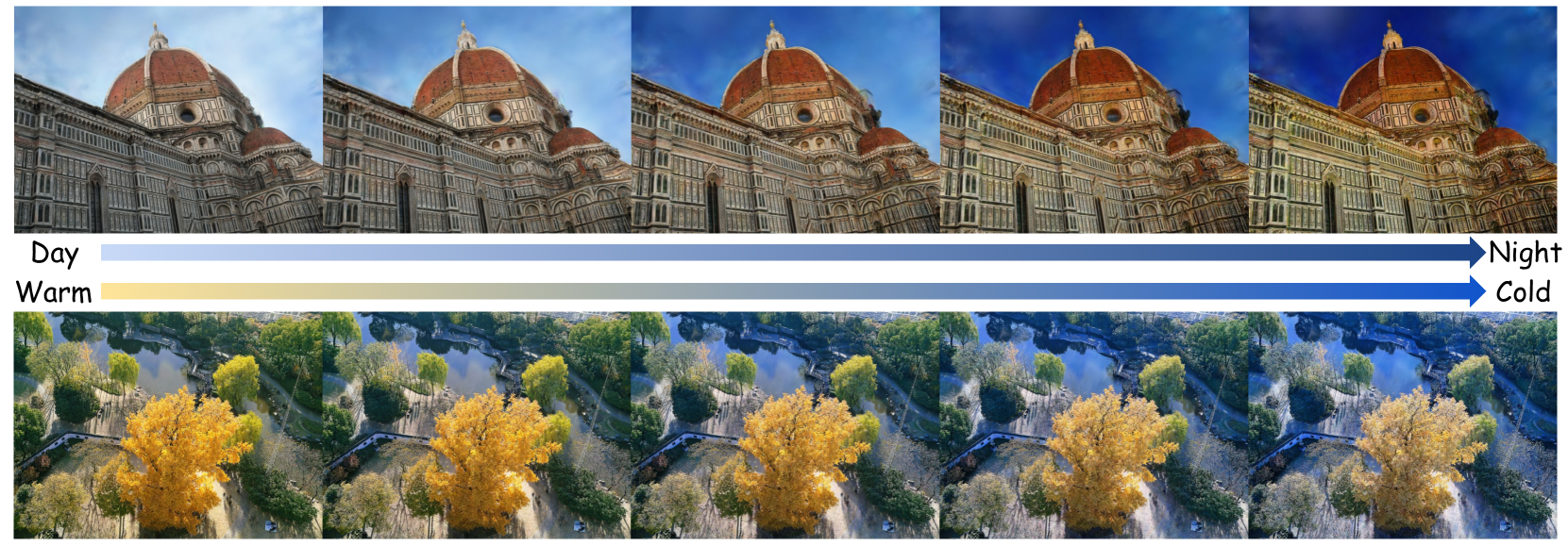
### Visual Description
## Image Sequence: Day/Night and Warm/Cold Color Grading
### Overview
The image presents a sequence of photographs depicting two different scenes (a cathedral and a park) under varying color grading conditions. The sequence progresses from left to right, transitioning from daytime/warm tones to nighttime/cold tones. The color grading is indicated by two color gradients with labels "Day" to "Night" and "Warm" to "Cold".
### Components/Axes
* **Scenes:**
* Top Row: Cathedral (likely the Florence Cathedral)
* Bottom Row: Park scene with a pond and trees
* **Color Gradients:**
* Top Gradient: Light blue transitioning to dark blue, labeled "Day" (left) and "Night" (right) with an arrow indicating the direction of change.
* Bottom Gradient: Light yellow transitioning to dark blue, labeled "Warm" (left) and "Cold" (right) with an arrow indicating the direction of change.
### Detailed Analysis or ### Content Details
The image is divided into three horizontal sections: the cathedral images, the color gradients, and the park images.
**Cathedral Images:**
* There are five images of the cathedral, each with a different color grading.
* From left to right, the images transition from a bright, warm tone to a darker, cooler tone.
* The first image has a light blue sky and warm lighting on the cathedral.
* The last image has a dark blue sky and cooler lighting on the cathedral.
**Color Gradients:**
* The color gradients visually represent the transition from day to night and warm to cold.
* The gradients are positioned between the cathedral and park images, providing a visual key for the color grading applied to each scene.
**Park Images:**
* There are five images of the park, each with a different color grading corresponding to the cathedral images above.
* From left to right, the images transition from a bright, warm tone to a darker, cooler tone.
* The first image has warm, yellow tones in the trees and a light blue sky.
* The last image has cooler, blue tones in the trees and a darker blue sky.
### Key Observations
* The color grading is consistent across both the cathedral and park scenes.
* The transition from warm to cold tones is gradual and visually apparent.
* The color gradients provide a clear visual representation of the color grading applied to each image.
### Interpretation
The image demonstrates the effect of different color grading techniques on two distinct scenes. The transition from daytime/warm tones to nighttime/cold tones is visually striking and effectively conveys the impact of color grading on the overall mood and atmosphere of the images. The color gradients serve as a key to understanding the color grading applied to each image, making it easy to compare and contrast the different effects. The image is likely intended to showcase the capabilities of color grading software or techniques.
</details>
Figure 12: Visualization of appearance code interpolation. We show five test views from the Phototourism [67] dataset (top) and a self-captured tree scene (bottom) with linearly-interpolated appearance codes.
V-C Ablation Studies
In this section, we ablate each individual module to validate their effectiveness. We select all scenes from the Mip-NeRF360 [50] dataset as quantitative comparison, given its representative characteristics. Additionally, we select Block_Small from the MatrixCity [1] dataset for qualitative comparison. In this section, we ablate each individual module to verify their effectiveness. Meanwhile, we choose the octree-version of Scaffold-GS as the full model, with the vanilla Scaffold-GS serving as the baseline for comparison. Quantitative and qualitative results can be found in Tab. VII and Fig. 13.
V-C 1 Next Level Grow Operator
To evaluate the effectiveness of next-level anchor growing, as detailed in Section IV-B, we conduct an ablation in which new anchors are only allowed to grow at the same LOD level. The results, presented in Tab. VII, show that while the number of rendered Gaussian primitives and storage requirements decreased, there was a significant decline in image visual quality. This suggests that incorporating finer anchors into higher LOD levels not only improves the capture of high-frequency details but also enhances the interaction between adjacent LOD levels.
V-C 2 LOD Bias
To validate its contribution to margin details, we ablate the proposed LOD bias. The results, presented in Tab. VII, indicates that LOD bias is essential for enhancing the rendering quality, particularly in regions rich in high-frequency details for smooth trajectories, which can be observed in column (a)(b) of Fig. 13, as the white stripes on the black buildings become continuous and complete.
V-C 3 Progressive Training
To compare its influence on LOD level overlapping, we ablate progressive training strategy. In column (a)(c) of Fig. 13, the building windows are clearly noticeable, indicating that the strategy contributes to reduce the rendered Gaussian redundancy and decouple the Gaussias of different scales in the scene to their corresponding LOD levels. In addition, the quantitative results also verify the improvement of scene reconstruction accuracy by the proposed strategy, as shown in Tab. VII.
V-C 4 View Frequency
Due to the design of the octree structure, anchors at higher LOD levels are only rendered and optimized when the camera view is close to them. These anchors are often not sufficiently optimized due to their limited number, leading to visual artifacts when rendering from novel views. We perform an ablation of the view frequency strategy during the anchor pruning stage, as described detailly in Sec. IV-B 2. Implementing this strategy eliminates floaters, particularly in close-up views, enhances visual quality, and significantly reduces storage requirements, as shown in Tab. VII and Fig. 4.
TABLE VII: Quantitative results on ablation studies. We list the rendering metrics for each ablation described in Sec. V-C.
| Scaffold-GS [3] Ours w/o $l_{next}$ grow. Ours w/o progressive. | 27.90 27.64 27.86 | 0.815 0.811 0.818 | 0.220 0.223 0.215 | 666/197.5M 594/99.7M 698/142.3M |
| --- | --- | --- | --- | --- |
| Ours w/o LOD bias | 27.85 | 0.818 | 0.214 | 667/146.8M |
| Ours w/o view freq. | 27.74 | 0.817 | 0.211 | 765/244.4M |
| Our-Scaffold-GS | 28.05 | 0.819 | 0.214 | 657/139.6M |
<details>
<summary>x13.png Details</summary>
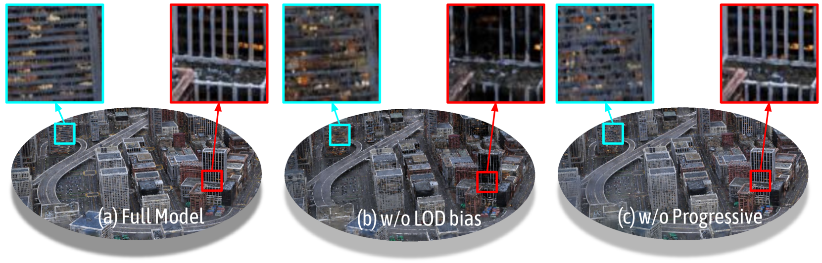
### Visual Description
## Image Comparison: Rendering Techniques
### Overview
The image presents a visual comparison of three different rendering techniques applied to a cityscape model. Each technique is showcased with a wide view of the city and two zoomed-in views, one highlighted with a cyan box and the other with a red box. The techniques being compared are: (a) Full Model, (b) w/o LOD bias, and (c) w/o Progressive.
### Components/Axes
* **Titles:**
* (a) Full Model
* (b) w/o LOD bias
* (c) w/o Progressive
* **Zoomed-in Views:** Each rendering technique has two zoomed-in views associated with it. One is highlighted with a cyan box and the other with a red box.
### Detailed Analysis or Content Details
* **(a) Full Model:**
* The wide view shows a detailed cityscape with numerous buildings and roads.
* The cyan-boxed zoomed-in view shows a section of a building with visible window details.
* The red-boxed zoomed-in view shows a section of a building with vertical lines, possibly representing window frames or architectural details.
* **(b) w/o LOD bias:**
* The wide view shows a cityscape that appears slightly less detailed than the "Full Model" version.
* The cyan-boxed zoomed-in view shows a section of a building with blurred window details.
* The red-boxed zoomed-in view shows a section of a building with less defined vertical lines compared to the "Full Model" version.
* **(c) w/o Progressive:**
* The wide view shows a cityscape that appears similar in detail to the "Full Model" version.
* The cyan-boxed zoomed-in view shows a section of a building with visible window details, similar to the "Full Model" version.
* The red-boxed zoomed-in view shows a section of a building with vertical lines, similar to the "Full Model" version.
### Key Observations
* The "Full Model" rendering appears to have the highest level of detail in both the wide view and the zoomed-in views.
* The "w/o LOD bias" rendering seems to have reduced detail, particularly noticeable in the zoomed-in views where the window details are blurred and the vertical lines are less defined.
* The "w/o Progressive" rendering appears to maintain a similar level of detail to the "Full Model" rendering.
### Interpretation
The image demonstrates the impact of different rendering techniques on the visual quality of a cityscape model. The "Full Model" likely represents a baseline with all rendering features enabled. Removing the LOD (Level of Detail) bias results in a noticeable reduction in detail, suggesting that LOD bias is important for maintaining visual fidelity, especially in zoomed-in views. Removing the "Progressive" rendering feature seems to have little to no impact on the final image quality, at least in the areas highlighted. The comparison suggests that LOD bias plays a more significant role in rendering detail than the "Progressive" feature in this specific scenario.
</details>
Figure 13: Visualizations of the rendered images from (a) our full model, (b) ours w/o LOD bias, (c) ours w/o progressive training. As observed, LOD bias aids in restoring sharp building edges and lines, while progressive training helps recover the geometric structure from coarse to fine details.
VI Limitations and Conclusion
In this work, we introduce Level-of-Details (LOD) to Gaussian representation, using a novel octree structure to organize anchors hierarchically. Our model, Octree-GS, addresses previous limitations by dynamically fetching appropriate LOD levels based on observed views and scene complexity, ensuring consistent rendering performance with adaptive LOD adjustments. Through careful design, Octree-GS significantly enhances detail capture while maintaining real-time rendering performance without increasing the number of Gaussian primitives. This suggests potential for future real-world streaming experiences, demonstrating the capability of advanced rendering methods to deliver seamless, high-quality interactive 3D scene and content.
However, certain model components, like octree construction and progressive training, still require hyperparameter tuning. Balancing anchors in each LOD level and adjusting training iteration activation are also crucial. Moreover, our model still faces challenges associated with 3D-GS, including dependency on the precise camera poses and lack of geometry support. These are left as our future works.
VII Supplementary Material
The supplementary material includes quantitative results for each scene from the dataset used in the main text, covering image quality metrics such as PSNR, [64] and LPIPS [65], as well as the number of rendered Gaussian primitives and storage size.
TABLE VIII: PSNR for all scenes in the Mip-NeRF360 [50] dataset.
| Method Scenes 2D-GS [15] 3D-GS [5] | bicycle 24.77 25.10 | bonsai 31.42 32.19 | counter 28.20 29.22 | flowers 21.02 21.57 | garden 26.73 27.45 | kitchen 30.66 31.62 | room 30.95 31.53 | stump 26.17 26.70 | treehill 22.48 22.46 |
| --- | --- | --- | --- | --- | --- | --- | --- | --- | --- |
| Mip-Splatting [14] | 25.13 | 32.56 | 29.30 | 21.64 | 27.43 | 31.48 | 31.73 | 26.65 | 22.60 |
| Scaffold-GS [3] | 25.19 | 33.22 | 29.99 | 21.40 | 27.48 | 31.77 | 32.30 | 26.67 | 23.08 |
| Anchor-2D-GS | 24.81 | 31.01 | 28.44 | 21.25 | 26.65 | 30.35 | 31.08 | 26.52 | 22.72 |
| Anchor-3D-GS | 25.21 | 32.20 | 29.12 | 21.52 | 27.37 | 31.46 | 31.83 | 26.74 | 22.85 |
| Our-2D-GS | 24.89 | 30.85 | 28.56 | 21.19 | 26.88 | 30.22 | 31.17 | 26.62 | 22.78 |
| Our-3D-GS | 25.20 | 32.29 | 29.27 | 21.40 | 27.36 | 31.70 | 31.96 | 26.78 | 22.85 |
| Our-Scaffold-GS | 25.24 | 33.76 | 30.19 | 21.46 | 27.67 | 31.84 | 32.51 | 26.63 | 23.13 |
TABLE IX: SSIM for all scenes in the Mip-NeRF360 [50] dataset.
| Method Scenes 2D-GS [15] 3D-GS [5] | bicycle 0.730 0.747 | bonsai 0.935 0.947 | counter 0.899 0.917 | flowers 0.568 0.600 | garden 0.839 0.861 | kitchen 0.923 0.932 | room 0.916 0.926 | stump 0.759 0.773 | treehill 0.627 0.636 |
| --- | --- | --- | --- | --- | --- | --- | --- | --- | --- |
| Mip-Splatting [14] | 0.747 | 0.948 | 0.917 | 0.601 | 0.861 | 0.933 | 0.928 | 0.772 | 0.639 |
| Scaffold-GS [3] | 0.751 | 0.952 | 0.922 | 0.587 | 0.853 | 0.931 | 0.932 | 0.767 | 0.644 |
| Anchor-2D-GS | 0.735 | 0.933 | 0.900 | 0.575 | 0.838 | 0.917 | 0.917 | 0.762 | 0.630 |
| Anchor-3D-GS | 0.758 | 0.946 | 0.913 | 0.591 | 0.857 | 0.928 | 0.927 | 0.772 | 0.640 |
| Our-2D-GS | 0.737 | 0.932 | 0.903 | 0.572 | 0.838 | 0.918 | 0.919 | 0.763 | 0.630 |
| Our-3D-GS | 0.761 | 0.946 | 0.916 | 0.587 | 0.855 | 0.931 | 0.929 | 0.772 | 0.640 |
| Our-Scaffold-GS | 0.755 | 0.955 | 0.925 | 0.595 | 0.861 | 0.933 | 0.936 | 0.766 | 0.641 |
TABLE X: LPIPS for all scenes in the Mip-NeRF360 [50] dataset.
| Method Scenes 2D-GS [15] 3D-GS [5] | bicycle 0.284 0.243 | bonsai 0.204 0.178 | counter 0.214 0.179 | flowers 0.389 0.345 | garden 0.153 0.114 | kitchen 0.134 0.117 | room 0.218 0.196 | stump 0.279 0.231 | treehill 0.385 0.335 |
| --- | --- | --- | --- | --- | --- | --- | --- | --- | --- |
| Mip-Splatting [14] | 0.245 | 0.178 | 0.179 | 0.347 | 0.115 | 0.115 | 0.192 | 0.232 | 0.334 |
| Scaffold-GS [3] | 0.247 | 0.173 | 0.177 | 0.359 | 0.13 | 0.118 | 0.183 | 0.252 | 0.338 |
| Anchor-2D-GS | 0.262 | 0.200 | 0.203 | 0.376 | 0.146 | 0.140 | 0.209 | 0.261 | 0.371 |
| Anchor-3D-GS | 0.230 | 0.177 | 0.182 | 0.363 | 0.121 | 0.121 | 0.193 | 0.249 | 0.348 |
| Our-2D-GS | 0.262 | 0.205 | 0.198 | 0.378 | 0.148 | 0.140 | 0.205 | 0.264 | 0.374 |
| Our-3D-GS | 0.225 | 0.178 | 0.176 | 0.364 | 0.125 | 0.116 | 0.190 | 0.250 | 0.357 |
| Our-Scaffold-GS | 0.235 | 0.164 | 0.169 | 0.347 | 0.116 | 0.115 | 0.172 | 0.250 | 0.360 |
TABLE XI: Number of Gaussian Primitives(#K) for all scenes in the Mip-NeRF360 [50] dataset.
| Method Scenes 2D-GS [15] 3D-GS [5] | bicycle 555 1453 | bonsai 210 402 | counter 232 530 | flowers 390 907 | garden 749 2030 | kitchen 440 1034 | room 199 358 | stump 413 932 | treehill 383 785 |
| --- | --- | --- | --- | --- | --- | --- | --- | --- | --- |
| Mip-Splatting [14] | 1584 | 430 | 545 | 950 | 2089 | 1142 | 405 | 1077 | 892 |
| Scaffold-GS [3] | 764 | 532 | 377 | 656 | 1121 | 905 | 272 | 637 | 731 |
| Anchor-2D-GS | 887 | 337 | 353 | 548 | 938 | 466 | 270 | 587 | 540 |
| Anchor-3D-GS | 1187 | 370 | 388 | 634 | 1524 | 535 | 293 | 647 | 781 |
| Our-2D-GS | 540 | 259 | 294 | 428 | 718 | 414 | 184 | 394 | 344 |
| Our-3D-GS | 659 | 301 | 334 | 478 | 987 | 710 | 195 | 436 | 433 |
| Our-Scaffold-GS | 653 | 631 | 409 | 675 | 1475 | 777 | 374 | 549 | 372 |
TABLE XII: Storage memory(#MB) for all scenes in the Mip-NeRF360 [50] dataset.
| Method Scenes 2D-GS [15] 3D-GS [5] | bicycle 889.6 1361.8 | bonsai 173.1 293.5 | counter 135.4 293.3 | flowers 493.5 878.5 | garden 603.1 1490.6 | kitchen 191.0 413.1 | room 180.0 355.6 | stump 670.3 1115.2 | treehill 630.9 878.6 |
| --- | --- | --- | --- | --- | --- | --- | --- | --- | --- |
| Mip-Splatting [14] | 1433.6 | 318.1 | 307.5 | 970.2 | 1448.9 | 463.4 | 401.0 | 1239.0 | 964.3 |
| Scaffold-GS [3] | 340.2 | 133.3 | 90.4 | 243.8 | 231.7 | 102.2 | 86.1 | 294.2 | 256.0 |
| Anchor-2D-GS | 599.2 | 280.0 | 191.5 | 530.0 | 634.4 | 190.7 | 228.4 | 359.1 | 521.4 |
| Anchor-3D-GS | 765.5 | 301.7 | 204.9 | 656.1 | 988.6 | 217.0 | 244.6 | 417.4 | 632.2 |
| Our-2D-GS | 485.0 | 368.6 | 265.6 | 442.3 | 598.6 | 272.3 | 180.8 | 292.8 | 438.3 |
| Our-3D-GS | 648.6 | 382.7 | 305.8 | 487.7 | 706.2 | 282.9 | 162.7 | 322.1 | 468.4 |
| Our-Scaffold-GS | 216.0 | 133.5 | 83.2 | 198.3 | 236.3 | 88.7 | 83.5 | 141.9 | 104.4 |
TABLE XIII: Quantitative results for all scenes in the Tanks&Temples [60] dataset.
| Dataset Method Metrics 2D-GS [15] | Truck PSNR 25.12 | Train SSIM 0.870 | LPIPS 0.173 | #GS(k)/Mem 393/287.2M | PSNR 21.38 | SSIM 0.790 | LPIPS 0.251 | #GS(k)/Mem 310/121.5M |
| --- | --- | --- | --- | --- | --- | --- | --- | --- |
| 3D-GS [5] | 25.52 | 0.884 | 0.142 | 876/610.8M | 22.30 | 0.819 | 0.201 | 653/249.3M |
| Mip-Splatting [14] | 25.74 | 0.888 | 0.142 | 967/718.9M | 22.17 | 0.824 | 0.199 | 696/281.9M |
| Scaffold-GS [3] | 26.04 | 0.889 | 0.131 | 698/214.6M | 22.91 | 0.838 | 0.181 | 554/120.4M |
| Anchor-2D-GS | 25.45 | 0.873 | 0.161 | 472/349.7M | 21.58 | 0.797 | 0.237 | 457/208.3M |
| Anchor-3D-GS | 25.85 | 0.883 | 0.146 | 603/452.8M | 22.18 | 0.810 | 0.222 | 541/245.6M |
| Our-2D-GS | 25.32 | 0.872 | 0.158 | 304 /208.5M | 21.92 | 0.812 | 0.215 | 355 /173.9M |
| Our-3D-GS | 25.81 | 0.887 | 0.131 | 407/542.8M | 22.52 | 0.828 | 0.190 | 440/224.90M |
| Our-Scaffold-GS | 26.24 | 0.894 | 0.122 | 426/ 93.7M | 23.11 | 0.838 | 0.184 | 460/ 83.4M |
TABLE XIV: Quantitative results for all scenes in the DeepBlending [61] dataset.
| Dataset Method Metrics 2D-GS [15] | Dr Johnson PSNR 28.74 | Playroom SSIM 0.897 | LPIPS 0.257 | #GS(k)/Mem 232/393.8M | PSNR 29.89 | SSIM 0.900 | LPIPS 0.257 | #GS(k)/Mem 160/276.7M |
| --- | --- | --- | --- | --- | --- | --- | --- | --- |
| 3D-GS [5] | 29.09 | 0.900 | 0.242 | 472/818.9M | 29.83 | 0.905 | 0.241 | 324/592.3M |
| Mip-Splatting [14] | 29.08 | 0.900 | 0.241 | 512/911.6M | 30.03 | 0.902 | 0.245 | 307/562.0M |
| Scaffold-GS [3] | 29.73 | 0.910 | 0.235 | 232/145.0M | 30.83 | 0.907 | 0.242 | 182/106.0M |
| Anchor-2D-GS | 28.68 | 0.893 | 0.266 | 186/346.3M | 30.02 | 0.899 | 0.262 | 138/231.8M |
| Anchor-3D-GS | 29.23 | 0.897 | 0.267 | 141/242.3M | 30.08 | 0.901 | 0.252 | 159/303.4M |
| Our-2D-GS | 28.94 | 0.894 | 0.26 | 97/268.2M | 29.93 | 0.899 | 0.268 | 70/136.4M |
| Our-3D-GS | 29.27 | 0.900 | 0.251 | 95 /240.7M | 30.03 | 0.901 | 0.263 | 63 /119.2M |
| Our-Scaffold-GS | 29.83 | 0.909 | 0.237 | 124/ 92.46M | 31.15 | 0.914 | 0.245 | 100/ 50.91M |
TABLE XV: PSNR for all scenes in the BungeeNeRF [51] dataset.
| Method Scenes 2D-GS [15] 3D-GS [5] | Amsterdam 27.22 27.75 | Barcelona 27.01 27.55 | Bilbao 28.59 28.91 | Chicago 25.62 28.27 | Hollywood 26.43 26.25 | Pompidou 26.62 27.16 | Quebec 28.38 28.86 | Rome 26.95 27.56 |
| --- | --- | --- | --- | --- | --- | --- | --- | --- |
| Mip-Splatting [14] | 28.16 | 27.72 | 29.13 | 28.28 | 26.59 | 27.71 | 29.23 | 28.33 |
| Scaffold-GS [3] | 27.82 | 28.09 | 29.20 | 28.55 | 26.36 | 27.72 | 29.29 | 28.24 |
| Anchor-2D-GS | 26.80 | 27.03 | 28.02 | 27.50 | 25.68 | 26.87 | 28.21 | 27.32 |
| Anchor-3D-GS | 27.70 | 27.93 | 28.92 | 28.20 | 26.20 | 27.17 | 28.83 | 28.22 |
| Our-2D-GS | 27.14 | 27.28 | 28.24 | 27.78 | 26.13 | 26.58 | 28.07 | 27.47 |
| Our-3D-GS | 27.95 | 27.91 | 28.81 | 28.24 | 26.51 | 27.00 | 28.98 | 28.09 |
| Our-Scaffold-GS | 28.16 | 28.40 | 29.39 | 28.86 | 26.76 | 27.46 | 29.46 | 28.59 |
TABLE XVI: SSIM for all scenes in the BungeeNeRF [51] dataset.
| Method Scenes 2D-GS [15] 3D-GS [5] | Amsterdam 0.896 0.918 | Barcelona 0.907 0.919 | Bilbao 0.912 0.918 | Chicago 0.901 0.932 | Hollywood 0.872 0.873 | Pompidou 0.907 0.919 | Quebec 0.923 0.937 | Rome 0.902 0.918 |
| --- | --- | --- | --- | --- | --- | --- | --- | --- |
| Mip-Splatting [14] | 0.918 | 0.919 | 0.918 | 0.930 | 0.876 | 0.923 | 0.938 | 0.922 |
| Scaffold-GS [3] | 0.914 | 0.923 | 0.918 | 0.929 | 0.866 | 0.926 | 0.939 | 0.924 |
| Anchor-2D-GS | 0.872 | 0.887 | 0.886 | 0.897 | 0.838 | 0.900 | 0.910 | 0.891 |
| Anchor-3D-GS | 0.902 | 0.912 | 0.907 | 0.916 | 0.871 | 0.919 | 0.930 | 0.915 |
| Our-2D-GS | 0.887 | 0.894 | 0.892 | 0.912 | 0.857 | 0.893 | 0.911 | 0.895 |
| Our-3D-GS | 0.912 | 0.910 | 0.905 | 0.920 | 0.875 | 0.907 | 0.928 | 0.912 |
| Our-Scaffold-GS | 0.922 | 0.928 | 0.921 | 0.934 | 0.884 | 0.923 | 0.942 | 0.930 |
TABLE XVII: LPIPS for all scenes in the BungeeNeRF [51] dataset.
| Method Scenes 2D-GS [15] 3D-GS [5] | Amsterdam 0.132 0.092 | Barcelona 0.101 0.082 | Bilbao 0.109 0.092 | Chicago 0.13 0.080 | Hollywood 0.152 0.128 | Pompidou 0.109 0.090 | Quebec 0.113 0.087 | Rome 0.123 0.096 |
| --- | --- | --- | --- | --- | --- | --- | --- | --- |
| Mip-Splatting [14] | 0.094 | 0.082 | 0.095 | 0.081 | 0.130 | 0.087 | 0.087 | 0.093 |
| Scaffold-GS [3] | 0.102 | 0.078 | 0.090 | 0.08 | 0.157 | 0.082 | 0.080 | 0.087 |
| Anchor-2D-GS | 0.156 | 0.125 | 0.137 | 0.125 | 0.196 | 0.119 | 0.127 | 0.131 |
| Anchor-3D-GS | 0.127 | 0.099 | 0.119 | 0.105 | 0.160 | 0.100 | 0.100 | 0.105 |
| Our-2D-GS | 0.139 | 0.112 | 0.131 | 0.103 | 0.169 | 0.126 | 0.125 | 0.128 |
| Our-3D-GS | 0.105 | 0.094 | 0.115 | 0.095 | 0.146 | 0.113 | 0.100 | 0.108 |
| Our-Scaffold-GS | 0.090 | 0.071 | 0.091 | 0.077 | 0.128 | 0.089 | 0.081 | 0.080 |
TABLE XVIII: Number of Gaussian Primitives(#K) for all scenes in the BungeeNeRF [51] dataset.
| Method Scenes 2D-GS [15] 3D-GS [5] | Amsterdam 1026 2358 | Barcelona 1251 3106 | Bilbao 968 2190 | Chicago 1008 2794 | Hollywood 1125 2812 | Pompidou 1526 3594 | Quebec 811 2176 | Rome 914 2459 |
| --- | --- | --- | --- | --- | --- | --- | --- | --- |
| Mip-Splatting [14] | 2325 | 2874 | 2072 | 2712 | 2578 | 3233 | 1969 | 2251 |
| Scaffold-GS [3] | 1219 | 1687 | 1122 | 1958 | 1117 | 2600 | 1630 | 1886 |
| Anchor-2D-GS | 1222 | 1050 | 1054 | 1168 | 706 | 1266 | 881 | 1050 |
| Anchor-3D-GS | 1842 | 1630 | 1393 | 1593 | 1061 | 1995 | 1368 | 1641 |
| Our-2D-GS | 703 | 771 | 629 | 631 | 680 | 786 | 582 | 629 |
| Our-3D-GS | 1094 | 1090 | 760 | 830 | 975 | 1120 | 816 | 932 |
| Our-Scaffold-GS | 1508 | 1666 | 1296 | 1284 | 1478 | 1584 | 1354 | 1622 |
TABLE XIX: Storage memory(#MB) for all scenes in the BungeeNeRF [51] dataset.
| Method Scenes 2D-GS [15] 3D-GS [5] | Amsterdam 809.6 1569.1 | Barcelona 1027.7 2191.9 | Bilbao 952.2 1446.1 | Chicago 633.2 1630.2 | Hollywood 814.3 1758.3 | Pompidou 1503.4 2357.6 | Quebec 643.2 1573.7 | Rome 705.5 1811.8 |
| --- | --- | --- | --- | --- | --- | --- | --- | --- |
| Mip-Splatting [14] | 1464.3 | 1935.4 | 1341.4 | 1536.0 | 1607.7 | 2037.8 | 1382.4 | 1577.0 |
| Scaffold-GS [3] | 236.2 | 378.8 | 219.0 | 306.1 | 208.3 | 478.5 | 340.2 | 386.6 |
| Anchor-2D-GS | 559.6 | 564.5 | 520.3 | 567.9 | 411.6 | 629.1 | 479.5 | 537.9 |
| Anchor-3D-GS | 866.4 | 862.8 | 699.4 | 778.5 | 607.9 | 979.3 | 725.3 | 802.5 |
| Our-2D-GS | 449.8 | 1014.4 | 425.9 | 1127.8 | 776.2 | 765.52 | 498.8 | 830.2 |
| Our-3D-GS | 1213.5 | 1414.3 | 892.4 | 1268.5 | 960.5 | 949.8 | 618.5 | 1048.3 |
| Our-Scaffold-GS | 273.8 | 355.9 | 246.5 | 286.8 | 259.0 | 339.6 | 258.8 | 353.4 |
TABLE XX: PSNR for multi-resolution Mip-NeRF360 [50] scenes (1 $×$ resolution).
| 3D-GS [5] Mip-Splatting [14] Scaffold-GS [3] | 23.66 25.19 23.64 | 29.89 31.76 31.31 | 27.98 29.07 28.82 | 20.42 21.68 20.87 | 25.45 26.82 26.04 | 29.55 31.27 30.39 | 30.51 31.60 31.36 | 25.48 26.71 25.66 | 22.50 22.74 23.14 |
| --- | --- | --- | --- | --- | --- | --- | --- | --- | --- |
| Our-Scaffold-GS | 24.21 | 33.44 | 30.15 | 20.89 | 27.01 | 31.83 | 32.39 | 25.92 | 23.26 |
TABLE XXI: SSIM for multi-resolution Mip-NeRF360 [50] scenes (1 $×$ resolution).
| 3D-GS [5] Mip-Splatting [14] Scaffold-GS [3] | 0.648 0.730 0.640 | 0.917 0.939 0.932 | 0.883 0.904 0.895 | 0.510 0.586 0.521 | 0.752 0.817 0.772 | 0.902 0.924 0.910 | 0.905 0.919 0.916 | 0.707 0.764 0.709 | 0.587 0.622 0.605 |
| --- | --- | --- | --- | --- | --- | --- | --- | --- | --- |
| Our-Scaffold-GS | 0.676 | 0.952 | 0.919 | 0.541 | 0.823 | 0.930 | 0.932 | 0.722 | 0.628 |
TABLE XXII: LPIPS for multi-resolution Mip-NeRF360 [50] scenes (1 $×$ resolution).
| 3D-GS [5] Mip-Splatting [14] Scaffold-GS [3] | 0.359 0.275 0.355 | 0.223 0.188 0.208 | 0.235 0.196 0.219 | 0.443 0.367 0.430 | 0.269 0.190 0.242 | 0.167 0.130 0.159 | 0.242 0.214 0.219 | 0.331 0.258 0.326 | 0.440 0.379 0.407 |
| --- | --- | --- | --- | --- | --- | --- | --- | --- | --- |
| Our-Scaffold-GS | 0.313 | 0.169 | 0.178 | 0.401 | 0.168 | 0.119 | 0.186 | 0.309 | 0.364 |
TABLE XXIII: PSNR for multi-resolution Mip-NeRF360 [50] scenes (2 $×$ resolution).
| 3D-GS [5] Mip-Splatting [14] Scaffold-GS [3] | 25.41 26.83 25.43 | 27.56 28.80 28.37 | 26.42 27.57 26.60 | 31.29 32.44 32.36 | 28.57 29.59 29.52 | 30.54 32.27 31.50 | 30.71 32.41 32.20 | 21.83 23.22 22.36 | 23.67 23.90 24.51 |
| --- | --- | --- | --- | --- | --- | --- | --- | --- | --- |
| Our-Scaffold-GS | 25.92 | 29.08 | 26.81 | 33.31 | 30.77 | 32.44 | 34.13 | 22.38 | 24.53 |
TABLE XXIV: SSIM for multi-resolution Mip-NeRF360 [50] scenes (2 $×$ resolution).
| 3D-GS [5] Mip-Splatting [14] Scaffold-GS [3] | 0.756 0.823 0.759 | 0.866 0.902 0.883 | 0.769 0.819 0.773 | 0.933 0.946 0.946 | 0.904 0.923 0.918 | 0.935 0.950 0.941 | 0.939 0.956 0.953 | 0.620 0.693 0.640 | 0.676 0.705 0.701 |
| --- | --- | --- | --- | --- | --- | --- | --- | --- | --- |
| Our-Scaffold-GS | 0.785 | 0.903 | 0.781 | 0.956 | 0.937 | 0.949 | 0.966 | 0.657 | 0.714 |
TABLE XXV: LPIPS for multi-resolution Mip-NeRF360 [50] scenes (2 $×$ resolution).
| 3D-GS [5] Mip-Splatting [14] Scaffold-GS [3] | 0.261 0.177 0.245 | 0.138 0.084 0.110 | 0.239 0.170 0.234 | 0.134 0.110 0.108 | 0.141 0.110 0.125 | 0.093 0.067 0.086 | 0.114 0.088 0.099 | 0.351 0.276 0.335 | 0.349 0.284 0.307 |
| --- | --- | --- | --- | --- | --- | --- | --- | --- | --- |
| Our-Scaffold-GS | 0.210 | 0.080 | 0.221 | 0.087 | 0.095 | 0.068 | 0.071 | 0.304 | 0.274 |
TABLE XXVI: PSNR for multi-resolution Mip-NeRF360 [50] scenes (4 $×$ resolution).
| 3D-GS [5] Mip-Splatting [14] Scaffold-GS [3] | 27.06 28.66 27.34 | 29.19 30.69 30.40 | 27.77 29.12 28.11 | 31.75 33.29 33.03 | 29.29 30.44 30.42 | 31.51 33.40 32.55 | 31.25 33.25 32.83 | 24.04 25.66 24.72 | 25.12 25.53 26.31 |
| --- | --- | --- | --- | --- | --- | --- | --- | --- | --- |
| Our-Scaffold-GS | 28.00 | 31.23 | 28.36 | 34.01 | 31.60 | 33.39 | 34.86 | 24.66 | 26.27 |
TABLE XXVII: SSIM for multi-resolution Mip-NeRF360 [50] scenes (4 $×$ resolution).
| 3D-GS [5] Mip-Splatting [14] Scaffold-GS [3] | 0.857 0.901 0.868 | 0.921 0.945 0.936 | 0.841 0.882 0.852 | 0.954 0.965 0.966 | 0.929 0.943 0.942 | 0.958 0.967 0.963 | 0.953 0.968 0.966 | 0.753 0.807 0.776 | 0.788 0.811 0.815 |
| --- | --- | --- | --- | --- | --- | --- | --- | --- | --- |
| Our-Scaffold-GS | 0.883 | 0.945 | 0.857 | 0.971 | 0.952 | 0.966 | 0.975 | 0.782 | 0.822 |
TABLE XXVIII: LPIPS for multi-resolution Mip-NeRF360 [50] scenes (4 $×$ resolution).
| 3D-GS [5] Mip-Splatting [14] Scaffold-GS [3] | 0.140 0.085 0.118 | 0.062 0.040 0.048 | 0.149 0.102 0.138 | 0.066 0.050 0.047 | 0.081 0.063 0.069 | 0.045 0.038 0.039 | 0.059 0.043 0.045 | 0.227 0.177 0.204 | 0.220 0.183 0.185 |
| --- | --- | --- | --- | --- | --- | --- | --- | --- | --- |
| Our-Scaffold-GS | 0.101 | 0.039 | 0.131 | 0.039 | 0.054 | 0.036 | 0.032 | 0.182 | 0.168 |
TABLE XXIX: PSNR for multi-resolution Mip-NeRF360 [50] scenes (8 $×$ resolution).
| 3D-GS [5] Mip-Splatting [14] Scaffold-GS [3] | 26.26 29.80 27.29 | 29.28 31.93 30.26 | 27.50 30.78 28.61 | 30.45 33.60 31.51 | 28.14 31.11 29.67 | 29.86 33.74 30.84 | 29.25 33.38 30.61 | 24.33 27.95 24.99 | 25.62 27.13 27.04 |
| --- | --- | --- | --- | --- | --- | --- | --- | --- | --- |
| Our-Scaffold-GS | 29.09 | 32.61 | 29.05 | 34.24 | 32.35 | 34.35 | 35.42 | 25.83 | 27.69 |
TABLE XXX: SSIM for multi-resolution Mip-NeRF360 [50] scenes (8 $×$ resolution).
| 3D-GS [5] Mip-Splatting [14] Scaffold-GS [3] | 0.871 0.938 0.894 | 0.930 0.964 0.941 | 0.846 0.925 0.875 | 0.953 0.973 0.965 | 0.928 0.957 0.946 | 0.954 0.975 0.961 | 0.944 0.973 0.959 | 0.805 0.883 0.825 | 0.840 0.886 0.871 |
| --- | --- | --- | --- | --- | --- | --- | --- | --- | --- |
| Our-Scaffold-GS | 0.919 | 0.964 | 0.885 | 0.978 | 0.964 | 0.977 | 0.981 | 0.838 | 0.885 |
TABLE XXXI: LPIPS for multi-resolution Mip-NeRF360 [50] scenes (8 $×$ resolution).
| 3D-GS [5] Mip-Splatting [14] Scaffold-GS [3] | 0.098 0.049 0.082 | 0.047 0.026 0.040 | 0.126 0.068 0.110 | 0.048 0.031 0.033 | 0.063 0.041 0.048 | 0.037 0.029 0.032 | 0.047 0.029 0.035 | 0.159 0.109 0.144 | 0.147 0.113 0.120 |
| --- | --- | --- | --- | --- | --- | --- | --- | --- | --- |
| Our-Scaffold-GS | 0.062 | 0.025 | 0.103 | 0.023 | 0.032 | 0.021 | 0.017 | 0.118 | 0.106 |
TABLE XXXII: Quantitative results for multi-resolution Tanks&Temples [60] dataset.
| 3D-GS [5] Mip-Splatting [14] Scaffold-GS [3] | 21.23 21.87 21.91 | 22.17 22.70 23.04 | 22.69 23.41 23.84 | 22.16 23.83 23.50 | 23.92 25.29 24.66 | 25.47 26.79 26.47 | 26.24 28.07 27.44 | 25.51 28.81 26.67 |
| --- | --- | --- | --- | --- | --- | --- | --- | --- |
| Our-Scaffold-GS | 22.49 | 23.50 | 24.18 | 24.22 | 25.85 | 27.53 | 28.83 | 29.67 |
| 3D-GS [5] Mip-Splatting [14] Scaffold-GS [3] | 0.754 0.791 0.781 | 0.830 0.859 0.860 | 0.879 0.906 0.907 | 0.880 0.929 0.913 | 0.827 0.868 0.844 | 0.899 0.925 0.916 | 0.930 0.955 0.946 | 0.929 0.969 0.945 |
| --- | --- | --- | --- | --- | --- | --- | --- | --- |
| Our-Scaffold-GS | 0.817 | 0.882 | 0.919 | 0.932 | 0.878 | 0.932 | 0.958 | 0.971 |
| 3D-GS [5] Mip-Splatting [14] Scaffold-GS [3] | 0.292 0.243 0.261 | 0.181 0.143 0.149 | 0.106 0.080 0.080 | 0.093 0.056 0.070 | 0.239 0.179 0.216 | 0.116 0.082 0.094 | 0.058 0.039 0.045 | 0.050 0.025 0.041 |
| --- | --- | --- | --- | --- | --- | --- | --- | --- |
| Our-Scaffold-GS | 0.216 | 0.119 | 0.068 | 0.055 | 0.154 | 0.066 | 0.033 | 0.023 |
TABLE XXXIII: Quantitative results for multi-resolution Deep Blending [61] dataset.
| 3D-GS [5] Mip-Splatting [14] Scaffold-GS [3] | 28.62 28.95 29.51 | 28.97 29.30 29.99 | 29.23 29.91 30.58 | 28.71 30.55 30.31 | 29.43 30.18 29.77 | 29.89 30.62 30.39 | 30.25 31.16 31.10 | 29.47 31.61 30.47 |
| --- | --- | --- | --- | --- | --- | --- | --- | --- |
| Our-Scaffold-GS | 29.75 | 30.14 | 30.58 | 30.92 | 30.87 | 31.42 | 31.76 | 31.63 |
| 3D-GS [5] Mip-Splatting [14] Scaffold-GS [3] | 0.890 0.900 0.900 | 0.900 0.911 0.914 | 0.911 0.925 0.930 | 0.907 0.936 0.932 | 0.898 0.909 0.900 | 0.919 0.929 0.923 | 0.935 0.946 0.944 | 0.934 0.956 0.949 |
| --- | --- | --- | --- | --- | --- | --- | --- | --- |
| Our-Scaffold-GS | 0.908 | 0.920 | 0.932 | 0.940 | 0.911 | 0.933 | 0.949 | 0.957 |
| 3D-GS [5] Mip-Splatting [14] Scaffold-GS [3] | 0.277 0.251 0.244 | 0.177 0.151 0.144 | 0.103 0.084 0.078 | 0.083 0.060 0.057 | 0.277 0.247 0.257 | 0.170 0.140 0.150 | 0.081 0.061 0.064 | 0.060 0.039 0.038 |
| --- | --- | --- | --- | --- | --- | --- | --- | --- |
| Our-Scaffold-GS | 0.263 | 0.159 | 0.082 | 0.061 | 0.274 | 0.164 | 0.068 | 0.041 |
References
- [1] Y. Li, L. Jiang, L. Xu, Y. Xiangli, Z. Wang, D. Lin, and B. Dai, “Matrixcity: A large-scale city dataset for city-scale neural rendering and beyond,” in Proceedings of the IEEE/CVF International Conference on Computer Vision, 2023, pp. 3205–3215.
- [2] B. Kerbl, A. Meuleman, G. Kopanas, M. Wimmer, A. Lanvin, and G. Drettakis, “A hierarchical 3d gaussian representation for real-time rendering of very large datasets,” ACM Transactions on Graphics (TOG), vol. 43, no. 4, pp. 1–15, 2024.
- [3] T. Lu, M. Yu, L. Xu, Y. Xiangli, L. Wang, D. Lin, and B. Dai, “Scaffold-gs: Structured 3d gaussians for view-adaptive rendering,” arXiv preprint arXiv:2312.00109, 2023.
- [4] B. Mildenhall, P. P. Srinivasan, M. Tancik, J. T. Barron, R. Ramamoorthi, and R. Ng, “Nerf: Representing scenes as neural radiance fields for view synthesis,” Communications of the ACM, vol. 65, no. 1, pp. 99–106, 2021.
- [5] B. Kerbl, G. Kopanas, T. Leimkühler, and G. Drettakis, “3d gaussian splatting for real-time radiance field rendering,” ACM Transactions on Graphics, vol. 42, no. 4, 2023.
- [6] W. Zielonka, T. Bagautdinov, S. Saito, M. Zollhöfer, J. Thies, and J. Romero, “Drivable 3d gaussian avatars,” arXiv preprint arXiv:2311.08581, 2023.
- [7] S. Saito, G. Schwartz, T. Simon, J. Li, and G. Nam, “Relightable gaussian codec avatars,” arXiv preprint arXiv:2312.03704, 2023.
- [8] S. Zheng, B. Zhou, R. Shao, B. Liu, S. Zhang, L. Nie, and Y. Liu, “Gps-gaussian: Generalizable pixel-wise 3d gaussian splatting for real-time human novel view synthesis,” arXiv preprint arXiv:2312.02155, 2023.
- [9] S. Qian, T. Kirschstein, L. Schoneveld, D. Davoli, S. Giebenhain, and M. Nießner, “Gaussianavatars: Photorealistic head avatars with rigged 3d gaussians,” arXiv preprint arXiv:2312.02069, 2023.
- [10] Y. Yan, H. Lin, C. Zhou, W. Wang, H. Sun, K. Zhan, X. Lang, X. Zhou, and S. Peng, “Street gaussians for modeling dynamic urban scenes,” arXiv preprint arXiv:2401.01339, 2024.
- [11] X. Zhou, Z. Lin, X. Shan, Y. Wang, D. Sun, and M.-H. Yang, “Drivinggaussian: Composite gaussian splatting for surrounding dynamic autonomous driving scenes,” arXiv preprint arXiv:2312.07920, 2023.
- [12] Y. Jiang, C. Yu, T. Xie, X. Li, Y. Feng, H. Wang, M. Li, H. Lau, F. Gao, Y. Yang et al., “Vr-gs: A physical dynamics-aware interactive gaussian splatting system in virtual reality,” arXiv preprint arXiv:2401.16663, 2024.
- [13] T. Xie, Z. Zong, Y. Qiu, X. Li, Y. Feng, Y. Yang, and C. Jiang, “Physgaussian: Physics-integrated 3d gaussians for generative dynamics,” arXiv preprint arXiv:2311.12198, 2023.
- [14] Z. Yu, A. Chen, B. Huang, T. Sattler, and A. Geiger, “Mip-splatting: Alias-free 3d gaussian splatting,” arXiv preprint arXiv:2311.16493, 2023.
- [15] B. Huang, Z. Yu, A. Chen, A. Geiger, and S. Gao, “2d gaussian splatting for geometrically accurate radiance fields,” in ACM SIGGRAPH 2024 Conference Papers, 2024, pp. 1–11.
- [16] L. Xu, V. Agrawal, W. Laney, T. Garcia, A. Bansal, C. Kim, S. Rota Bulò, L. Porzi, P. Kontschieder, A. Božič et al., “Vr-nerf: High-fidelity virtualized walkable spaces,” in SIGGRAPH Asia 2023 Conference Papers, 2023, pp. 1–12.
- [17] A. Yu, R. Li, M. Tancik, H. Li, R. Ng, and A. Kanazawa, “Plenoctrees for real-time rendering of neural radiance fields,” in Proceedings of the IEEE/CVF International Conference on Computer Vision, 2021, pp. 5752–5761.
- [18] J. N. Martel, D. B. Lindell, C. Z. Lin, E. R. Chan, M. Monteiro, and G. Wetzstein, “Acorn: Adaptive coordinate networks for neural scene representation,” arXiv preprint arXiv:2105.02788, 2021.
- [19] Y. Liu, H. Guan, C. Luo, L. Fan, J. Peng, and Z. Zhang, “Citygaussian: Real-time high-quality large-scale scene rendering with gaussians,” arXiv preprint arXiv:2404.01133, 2024.
- [20] L. Liu, J. Gu, K. Zaw Lin, T.-S. Chua, and C. Theobalt, “Neural sparse voxel fields,” Advances in Neural Information Processing Systems, vol. 33, pp. 15 651–15 663, 2020.
- [21] S. Fridovich-Keil, A. Yu, M. Tancik, Q. Chen, B. Recht, and A. Kanazawa, “Plenoxels: Radiance fields without neural networks,” in Proceedings of the IEEE/CVF Conference on Computer Vision and Pattern Recognition, 2022, pp. 5501–5510.
- [22] C. Sun, M. Sun, and H.-T. Chen, “Direct voxel grid optimization: Super-fast convergence for radiance fields reconstruction,” in Proceedings of the IEEE/CVF Conference on Computer Vision and Pattern Recognition, 2022, pp. 5459–5469.
- [23] A. Chen, Z. Xu, A. Geiger, J. Yu, and H. Su, “Tensorf: Tensorial radiance fields,” in European Conference on Computer Vision. Springer, 2022, pp. 333–350.
- [24] T. Müller, A. Evans, C. Schied, and A. Keller, “Instant neural graphics primitives with a multiresolution hash encoding,” ACM Transactions on Graphics (ToG), vol. 41, no. 4, pp. 1–15, 2022.
- [25] L. Xu, Y. Xiangli, S. Peng, X. Pan, N. Zhao, C. Theobalt, B. Dai, and D. Lin, “Grid-guided neural radiance fields for large urban scenes,” in Proceedings of the IEEE/CVF Conference on Computer Vision and Pattern Recognition, 2023, pp. 8296–8306.
- [26] Y. Xiangli, L. Xu, X. Pan, N. Zhao, B. Dai, and D. Lin, “Assetfield: Assets mining and reconfiguration in ground feature plane representation,” arXiv preprint arXiv:2303.13953, 2023.
- [27] H. Turki, M. Zollhöfer, C. Richardt, and D. Ramanan, “Pynerf: Pyramidal neural radiance fields,” Advances in Neural Information Processing Systems, vol. 36, 2024.
- [28] Z. Li, T. Müller, A. Evans, R. H. Taylor, M. Unberath, M.-Y. Liu, and C.-H. Lin, “Neuralangelo: High-fidelity neural surface reconstruction,” in Proceedings of the IEEE/CVF Conference on Computer Vision and Pattern Recognition, 2023, pp. 8456–8465.
- [29] C. Reiser, S. Garbin, P. P. Srinivasan, D. Verbin, R. Szeliski, B. Mildenhall, J. T. Barron, P. Hedman, and A. Geiger, “Binary opacity grids: Capturing fine geometric detail for mesh-based view synthesis,” arXiv preprint arXiv:2402.12377, 2024.
- [30] J. T. Barron, B. Mildenhall, D. Verbin, P. P. Srinivasan, and P. Hedman, “Zip-nerf: Anti-aliased grid-based neural radiance fields,” arXiv preprint arXiv:2304.06706, 2023.
- [31] J. Tang, J. Ren, H. Zhou, Z. Liu, and G. Zeng, “Dreamgaussian: Generative gaussian splatting for efficient 3d content creation,” arXiv preprint arXiv:2309.16653, 2023.
- [32] Y. Liang, X. Yang, J. Lin, H. Li, X. Xu, and Y. Chen, “Luciddreamer: Towards high-fidelity text-to-3d generation via interval score matching,” arXiv preprint arXiv:2311.11284, 2023.
- [33] J. Tang, Z. Chen, X. Chen, T. Wang, G. Zeng, and Z. Liu, “Lgm: Large multi-view gaussian model for high-resolution 3d content creation,” arXiv preprint arXiv:2402.05054, 2024.
- [34] Y. Feng, X. Feng, Y. Shang, Y. Jiang, C. Yu, Z. Zong, T. Shao, H. Wu, K. Zhou, C. Jiang et al., “Gaussian splashing: Dynamic fluid synthesis with gaussian splatting,” arXiv preprint arXiv:2401.15318, 2024.
- [35] J. Luiten, G. Kopanas, B. Leibe, and D. Ramanan, “Dynamic 3d gaussians: Tracking by persistent dynamic view synthesis,” arXiv preprint arXiv:2308.09713, 2023.
- [36] Z. Yang, X. Gao, W. Zhou, S. Jiao, Y. Zhang, and X. Jin, “Deformable 3d gaussians for high-fidelity monocular dynamic scene reconstruction,” arXiv preprint arXiv:2309.13101, 2023.
- [37] Y.-H. Huang, Y.-T. Sun, Z. Yang, X. Lyu, Y.-P. Cao, and X. Qi, “Sc-gs: Sparse-controlled gaussian splatting for editable dynamic scenes,” arXiv preprint arXiv:2312.14937, 2023.
- [38] V. Yugay, Y. Li, T. Gevers, and M. R. Oswald, “Gaussian-slam: Photo-realistic dense slam with gaussian splatting,” arXiv preprint arXiv:2312.10070, 2023.
- [39] N. Keetha, J. Karhade, K. M. Jatavallabhula, G. Yang, S. Scherer, D. Ramanan, and J. Luiten, “Splatam: Splat, track & map 3d gaussians for dense rgb-d slam,” arXiv preprint arXiv:2312.02126, 2023.
- [40] Q. Xu, Z. Xu, J. Philip, S. Bi, Z. Shu, K. Sunkavalli, and U. Neumann, “Point-nerf: Point-based neural radiance fields,” in Proceedings of the IEEE/CVF Conference on Computer Vision and Pattern Recognition, 2022, pp. 5438–5448.
- [41] S. Fridovich-Keil, G. Meanti, F. R. Warburg, B. Recht, and A. Kanazawa, “K-planes: Explicit radiance fields in space, time, and appearance,” in Proceedings of the IEEE/CVF Conference on Computer Vision and Pattern Recognition, 2023, pp. 12 479–12 488.
- [42] A. Cao and J. Johnson, “Hexplane: A fast representation for dynamic scenes,” in Proceedings of the IEEE/CVF Conference on Computer Vision and Pattern Recognition, 2023, pp. 130–141.
- [43] S. M. Rubin and T. Whitted, “A 3-dimensional representation for fast rendering of complex scenes,” in Proceedings of the 7th annual conference on Computer graphics and interactive techniques, 1980, pp. 110–116.
- [44] S. Laine and T. Karras, “Efficient sparse voxel octrees–analysis, extensions, and implementation,” NVIDIA Corporation, vol. 2, no. 6, 2010.
- [45] H. Bai, Y. Lin, Y. Chen, and L. Wang, “Dynamic plenoctree for adaptive sampling refinement in explicit nerf,” in Proceedings of the IEEE/CVF International Conference on Computer Vision, 2023, pp. 8785–8795.
- [46] Y. Verdie, F. Lafarge, and P. Alliez, “LOD Generation for Urban Scenes,” ACM Trans. on Graphics, vol. 34, no. 3, 2015.
- [47] H. Fang, F. Lafarge, and M. Desbrun, “Planar Shape Detection at Structural Scales,” in Proc. of the IEEE conference on Computer Vision and Pattern Recognition (CVPR), Salt Lake City, US, 2018.
- [48] M. Yu and F. Lafarge, “Finding Good Configurations of Planar Primitives in Unorganized Point Clouds,” in Proc. of the IEEE conference on Computer Vision and Pattern Recognition (CVPR), New Orleans, US, 2022.
- [49] J. T. Barron, B. Mildenhall, M. Tancik, P. Hedman, R. Martin-Brualla, and P. P. Srinivasan, “Mip-nerf: A multiscale representation for anti-aliasing neural radiance fields,” in Proceedings of the IEEE/CVF International Conference on Computer Vision, 2021, pp. 5855–5864.
- [50] J. T. Barron, B. Mildenhall, D. Verbin, P. P. Srinivasan, and P. Hedman, “Mip-nerf 360: Unbounded anti-aliased neural radiance fields,” in Proceedings of the IEEE/CVF Conference on Computer Vision and Pattern Recognition, 2022, pp. 5470–5479.
- [51] Y. Xiangli, L. Xu, X. Pan, N. Zhao, A. Rao, C. Theobalt, B. Dai, and D. Lin, “Bungeenerf: Progressive neural radiance field for extreme multi-scale scene rendering,” in European conference on computer vision. Springer, 2022, pp. 106–122.
- [52] J. Cui, J. Cao, Y. Zhong, L. Wang, F. Zhao, P. Wang, Y. Chen, Z. He, L. Xu, Y. Shi et al., “Letsgo: Large-scale garage modeling and rendering via lidar-assisted gaussian primitives,” arXiv preprint arXiv:2404.09748, 2024.
- [53] M. Zwicker, H. Pfister, J. Van Baar, and M. Gross, “Ewa volume splatting,” in Proceedings Visualization, 2001. VIS’01. IEEE, 2001, pp. 29–538.
- [54] J. L. Schonberger and J.-M. Frahm, “Structure-from-motion revisited,” in Proceedings of the IEEE conference on computer vision and pattern recognition, 2016, pp. 4104–4113.
- [55] H. Hoppe, “Progressive meshes,” in Seminal Graphics Papers: Pushing the Boundaries, Volume 2, 2023, pp. 111–120.
- [56] K. Park, U. Sinha, J. T. Barron, S. Bouaziz, D. B. Goldman, S. M. Seitz, and R. Martin-Brualla, “Nerfies: Deformable neural radiance fields,” in Proceedings of the IEEE/CVF International Conference on Computer Vision, 2021, pp. 5865–5874.
- [57] R. Martin-Brualla, N. Radwan, M. S. Sajjadi, J. T. Barron, A. Dosovitskiy, and D. Duckworth, “Nerf in the wild: Neural radiance fields for unconstrained photo collections,” in Proceedings of the IEEE/CVF Conference on Computer Vision and Pattern Recognition, 2021, pp. 7210–7219.
- [58] M. Tancik, V. Casser, X. Yan, S. Pradhan, B. Mildenhall, P. P. Srinivasan, J. T. Barron, and H. Kretzschmar, “Block-nerf: Scalable large scene neural view synthesis,” in Proceedings of the IEEE/CVF Conference on Computer Vision and Pattern Recognition, 2022, pp. 8248–8258.
- [59] P. Bojanowski, A. Joulin, D. Lopez-Paz, and A. Szlam, “Optimizing the latent space of generative networks,” arXiv preprint arXiv:1707.05776, 2017.
- [60] A. Knapitsch, J. Park, Q.-Y. Zhou, and V. Koltun, “Tanks and temples: Benchmarking large-scale scene reconstruction,” ACM Transactions on Graphics (ToG), vol. 36, no. 4, pp. 1–13, 2017.
- [61] P. Hedman, J. Philip, T. Price, J.-M. Frahm, G. Drettakis, and G. Brostow, “Deep blending for free-viewpoint image-based rendering,” ACM Transactions on Graphics (ToG), vol. 37, no. 6, pp. 1–15, 2018.
- [62] H. Turki, D. Ramanan, and M. Satyanarayanan, “Mega-nerf: Scalable construction of large-scale nerfs for virtual fly-throughs,” in Proceedings of the IEEE/CVF Conference on Computer Vision and Pattern Recognition, 2022, pp. 12 922–12 931.
- [63] L. Lin, Y. Liu, Y. Hu, X. Yan, K. Xie, and H. Huang, “Capturing, reconstructing, and simulating: the urbanscene3d dataset,” in European Conference on Computer Vision. Springer, 2022, pp. 93–109.
- [64] Z. Wang, A. C. Bovik, H. R. Sheikh, and E. P. Simoncelli, “Image quality assessment: from error visibility to structural similarity,” IEEE transactions on image processing, vol. 13, no. 4, pp. 600–612, 2004.
- [65] R. Zhang, P. Isola, A. A. Efros, E. Shechtman, and O. Wang, “The unreasonable effectiveness of deep features as a perceptual metric,” in Proceedings of the IEEE conference on computer vision and pattern recognition, 2018, pp. 586–595.
- [66] N. Snavely, S. M. Seitz, and R. Szeliski, “Photo tourism: exploring photo collections in 3d,” in ACM siggraph 2006 papers, 2006, pp. 835–846.
- [67] Y. Jin, D. Mishkin, A. Mishchuk, J. Matas, P. Fua, K. M. Yi, and E. Trulls, “Image matching across wide baselines: From paper to practice,” International Journal of Computer Vision, vol. 129, no. 2, pp. 517–547, 2021.