2403.19647v1

# Sparse Feature Circuits: Discovering and Editing Interpretable Causal Graphs in Language Models **Authors**: - Samuel Marks (Northeastern University) - &Can Rager - &Eric J. Michaud (MIT) - Yonatan Belinkov - Technion – IIT - &David Bau (Northeastern University) - &Aaron Mueller (Northeastern University) > Correspondence to and . ## Abstract We introduce methods for discovering and applying sparse feature circuits. These are causally implicated subnetworks of human-interpretable features for explaining language model behaviors. Circuits identified in prior work consist of polysemantic and difficult-to-interpret units like attention heads or neurons, rendering them unsuitable for many downstream applications. In contrast, sparse feature circuits enable detailed understanding of unanticipated mechanisms. Because they are based on fine-grained units, sparse feature circuits are useful for downstream tasks: We introduce Shift, where we improve the generalization of a classifier by ablating features that a human judges to be task-irrelevant. Finally, we demonstrate an entirely unsupervised and scalable interpretability pipeline by discovering thousands of sparse feature circuits for automatically discovered model behaviors. ## 1 Introduction The key challenge of interpretability research is to scalably explain the many unanticipated behaviors of neural networks (NNs). Much recent work explains NN behaviors in terms of coarse-grained model components, for example by implicating certain induction heads in in-context learning (Olsson et al., 2022) or MLP modules in factual recall (Meng et al., 2022; Geva et al., 2023; Nanda et al., 2023, inter alia). However, such components are generally polysemantic (Elhage et al., 2022) and hard to interpret, making it difficult to apply mechanistic insights to downstream applications. On the other hand, prior methods analyzing behaviors in terms of fine-grained units (Kim et al., 2018; Belinkov, 2022; Geiger et al., 2023; Zou et al., 2023) demand that researchers begin with the answer: they assume the existence of curated data that isolates the target behavior. Such approaches are not well-suited for discovering unanticipated mechanisms. We propose to explain model behaviors using fine-grained components that play narrow, interpretable roles. Doing so requires us to address two challenges: First, we must identify the correct fine-grained unit of analysis, since obvious choices like neurons We use “neuron” to refer to a basis-aligned direction in an LM’s latent space (not necessarily preceded by a nonlinearity). are rarely interpretable, and units discovered via supervised methods require pre-existing hypotheses. Second, we must address the scalability problem posed by searching for causal circuits over a large number of fine-grained units. We leverage recent progress in dictionary learning (Bricken et al., 2023; Cunningham et al., 2024) to tackle the first challenge. Namely, we train sparse autoencoders (SAEs) to identify directions in an LM’s latent space which represent human-interpretable features. Then, to solve the scalability challenge, we employ linear approximations (Sundararajan et al., 2017; Nanda, 2022; Syed et al., 2023) to efficiently identify SAE features which are most causally implicated in model behaviors, as well as connections between these features. The result is a sparse feature circuit which explains how model behaviors arise via interactions among fine-grained human-interpretable units. Sparse feature circuits can be productively used in downstream applications. We introduce a technique, Sparse Human-Interpretable Feature Trimming (Shift), which shifts the generalization of an LM classifier by surgically removing sensitivity to unintended signals—even without knowing what those signals are in advance. We demonstrate Shift by debiasing a classifier in a worst-case setting where an unintended signal (gender) is perfectly predictive of target labels (profession). Finally, we demonstrate our method’s scalability by automatically discovering thousands of LM behaviors with the clustering approach of Michaud et al. (2023), and then automatically discovering feature circuits for these behaviors. Figure 1: Overview. Given contrastive input pairs, classification data, or automatically discovered model behaviors, we discover circuits composed of human-interpretable sparse features to explain their underlying mechanisms. We then label each feature according to what it activates on or causes to happen. Finally, if desired, we can ablate spurious features out of the circuit to modify how the system generalizes. Our contributions are summarized as follows (Figure 1): 1. A scalable method to discover sparse feature circuits. We validate our method by evaluating feature circuits on a suite of subject-verb agreement tasks. 1. Shift, a technique for removing sensitivity to unintended signals without disambiguating data. 1. A fully-unsupervised automatic feature circuit discovery pipeline that identifies circuits for thousands of automatically discovered LM behaviors. We release code, data and autoencoders at github.com/saprmarks/feature-circuits. ## 2 Formulation #### Feature disentanglement with sparse autoencoders. A fundamental challenge in NN interpretability is that individual neurons are rarely interpretable (Elhage et al., 2022). Recently, Cunningham et al. (2024); Bricken et al. (2023) have shown that sparse autoencoders (SAEs) can be used to identify interpretable directions. We closely follow Bricken et al. (2023) to train SAEs for attention outputs, In other words, the output of the attention layer’s out projection. MLP outputs, and residual stream activations for each layer of Pythia-70M (Biderman et al., 2023). Given an input activation ${x}∈{ℝ}^d_model$ from one of these model components, the corresponding SAE computes a decomposition $$ {x}=\hat{{x}}+{\bm{ε}}({x})=∑_i=1^d_ SAEf_i({x}){v}_i+{b}+{\bm{ε}}({ x}) \tag{1} $$ into an approximate reconstruction $\hat{{x}}$ as a sparse sum of features ${v}_i$ and an SAE error term ${\bm{ε}}({x})∈{ℝ}^d_model$ . The features ${v}_i∈{ℝ}^d_model$ are unit vectors, the feature activations $f_i({x})∈{ℝ}$ are a sparse set of coefficients, ${b}∈{ℝ}^d_model$ is a bias, and we take $d_SAE=64· d_model$ . The SAEs are trained to minimize an L2 reconstruction error and an L1 regularization term which promotes sparsity. Details about our SAEs and their training can be found in Appendix B. Scalably training better SAEs is an active area of research, and we develop our methods with rapid future progress in mind. However, at present SAE errors ${\bm{ε}}({x})$ account for a relatively significant $1$ – $15\$ of the variance in ${x}$ . Our methods handle these SAE errors gracefully by incorporting them into our sparse feature circuits; this gives a principled decomposition of model behaviors into contributions from potentially-interpretable features and error components not yet captured by our SAEs. We additionally note that the main bottleneck to scaling our methods to larger models is the training of the SAEs themselves. As we expect increasing public availability of SAEs for large open-source models, we treat scaling SAEs themselves as out-of-scope and focus on the scalability of our core methods. #### Attributing causal effects with linear approximations. Let $m$ be a real-valued metric computed via a computation graph (e.g., a NN); let ${a}∈{ℝ}^d$ represent a node in this graph. Following prior work (Vig et al., 2020; Finlayson et al., 2021), we quantify the importance of ${a}$ on a pair of inputs $(x_clean,x_patch)$ via its indirect effect (IE; Pearl, 2001) on $m$ : $$ IE(m;{a};x_clean,x_patch)=m≤ft(x_ clean\middle|do({a}={a}_patch)\right)-m(x_clean). \tag{2} $$ Here ${a}_patch$ is the value that ${a}$ takes in the computation of $m(x_patch)$ , and $m(x_clean|do({a}={a}_patch))$ denotes the value of $m$ when computing $m(x_clean)$ but intervening in the computation of $m$ by manually setting ${a}$ to ${a}_patch$ . For example, given inputs $x_clean=$ “The teacher ” and $x_patch=$ “The teachers,” we have metric $m(x)=\log P(``{\color[rgb]{0.88671875,0.12890625,0.2734375\definecolor[ named]{pgfstrokecolor}{rgb}{0.88671875,0.12890625,0.2734375}are}''}|x)-\log P( ``{\color[rgb]{0.2421875,0.453125,0.8203125\definecolor[named]{ pgfstrokecolor}{rgb}{0.2421875,0.453125,0.8203125}is}''}|x)$ the log probability difference output by a LM. Then if ${a}$ is the activation of a particular neuron, a large value of $IE(m;{a};x_clean,x_patch)$ indicates that the neuron is highly influential on the model’s decision to output “is” vs. “are” on this pair of inputs. We often want to compute IEs for a very large number of model components ${a}$ , which cannot be done efficiently with (2). We thus employ linear approximations to (2) that can be computed for many ${a}$ in parallel. The simplest such approximation, attribution patching (Nanda, 2022; Syed et al., 2023; Kramár et al., 2024), employs a first-order Taylor expansion $$ \hat{IE}_atp(m;{a};x_clean,x_patch) =≤ft.∇_{a}m\right|_{a={a}_clean }≤ft({a}_patch-{a}_clean\right) \tag{3} $$ which estimates (2) for every ${a}$ in parallel using only two forward and one backward pass. In practice, since we use small models, we can instead employ a more expensive but more accurate approximation based on integrated gradients (Sundararajan et al., 2017): $$ \hat{IE}_ig(m;{a};x_clean,x_patch)= ≤ft(∑_α≤ft.∇_{a}m\right|_α{a_ clean+(1-α){a}_patch}\right)({a}_ patch-{a}_clean) \tag{4} $$ where the sum in (4) ranges over $N=10$ equally-equally spaced $α∈\{0,\tfrac{1}{N},\dots,\tfrac{N-1}{N}\}$ . This cannot be done in parallel for two nodes when one is downstream of another, but can be done in parallel for arbitrarily many nodes which do not depend on each other. Thus the additional cost of computing $\hat{IE}_ig$ over $\hat{IE}_atp$ scales linearly in $N$ and the serial depth of $m$ ’s computation graph. The above discussion applies to the setting where we have a pair of clean and patch inputs, and we would like to understand that effect of patching a particular node from its clean to patch values. But in some settings (§ 4, 5), we have only a single input $x$ . In this case, we instead approximate the indirect effect $IE(m;{a};x)=m(x|do({a}={0}))-m(x)$ of setting ${a}$ to ${0}$ . We get the modified formulas for $\hat{IE}(m;{a};x)$ from (3) and (4) by replacing ${a}$ with ${0}$ . ## 3 Sparse Feature Circuit Discovery In this section, we introduce sparse feature circuits, which are computational sub-graphs that explain model behaviors in terms of SAE features and error terms. We first explain our circuit discovery algorithm (§ 3.1). Then, we analyze circuits found with our technique to show that they are both more interpretable and more concise than circuits consisting of neurons (§ 3.2). Finally, we perform a case study of the circuits we discovered for two linguistic tasks related to subject-verb agreement (§ 3.3). ### 3.1 Method Figure 2: Overview of our method. We view our model as a computation graph that includes SAE features and errors. We cache activations (Step 1) and compute gradients (Step 2) for each node. We then compute approximate indirect effects with Eq. (3; shown) or (4) and filter according to a node threshold $T_N$ (Step 3). We similarly compute and filter edges (Step 4); see App. A.1. Suppose we are given an LM $M$ , SAEs for various submodules of $M$ (e.g., attention outputs, MLP outputs, and residual stream vectors, as in § 2), a dataset $D$ consisting either of contrastive pairs $(x_clean,x_patch)$ of inputs or of single inputs $x$ , and a metric $m$ depending on $M$ ’s output when processing data from $D$ . For example, Figure 2 shows the case where $D$ consists of pairs of inputs which differ in number, and $m$ is the log probability difference between $M$ outputting the verb form that is correct for the patch vs. clean input. Viewing SAE features as part of the model. A key idea underpinning our method is that, by applying the decomposition (1) to various hidden states ${x}$ in the LM, we can view the feature activations $f_i$ and SAE errors ${\bm{ε}}$ as being part of the LM’s computation. We can thus represent the model as a computation graph $G$ where nodes correspond to feature activations or SAE errors at particular token positions. Approximating the IE of each node. Let $\hat{IE}$ be one of $\hat{IE}_atp$ or $\hat{IE}_ig$ (see § 2). Then for each node ${a}$ in $G$ and input $x∼D$ , we compute $\hat{IE}(m;{a};x)$ . We apply some choice of node threshold $T_N$ to select nodes with a large (absolute) IE. Consistent with prior work (Nanda, 2022; Kramár et al., 2024), we find that $\hat{IE}_atp$ accurately estimates IEs for SAE features and SAE errors, with the exception of nodes in the layer 0 MLP and early residual stream layers, where $\hat{IE}_atp$ underestimates the true IE. We find that $\hat{IE}_ig$ significantly improves accuracy for these components, so we use it in our experiments below. See Appendix C for more information about linear approximation quality. Approximating the IE of edges. Using an analogous linear approximation, we also compute the average IE of edges in the computation graph. Although the idea is simple, the mathematics are somewhat involved, so we relegate the details to App. A.1. After computing these IEs, we filter for edges with absolute IE exceeding some edge threshold $T_E$ . Aggregation across token positions and examples. For templatic data where tokens in matching positions play consistent roles (see § 3.2, 3.3), we take the mean effect of nodes/edges across examples. For non-templatic data (§ 4, 5) we first sum the effects of corresponding nodes/edges across token position before taking the example-wise mean. See App. A.2. Practical considerations. Various practical difficulties arise for efficiently computing the gradients needed by our method. We solve using a combination of stop gradients, pass-through gradients, and tricks for efficient Jacobian-vector product computation; see App. A.3. ### 3.2 Discovering and Evaluating Sparse Feature Circuits for Subject–Verb Agreement To evaluate our method, we discover sparse feature circuits (henceforth, feature circuits) for four variants of the subject-verb agreement task (Table 1). Specifically, we adapt data from Finlayson et al. (2021) to produce datasets consisting of contrastive pairs of inputs that differ only in the grammatical number of the subject; the model’s task is to choose the appropriate verb inflection. We use this data along with our SAEs from § 2 to discover circuits for Pythia-70M. We evaluate circuits for interpretability, faithfulness, and completeness. For each criterion, we compare to neuron circuits discovered by applying our methods with neurons in place of sparse features; in this setting, there are no error terms ${\bm{ε}}$ . Interpretability. We asked human crowdworkers to rate the interpretability of random features, random neurons, features from our feature circuits, and neurons from our neuron circuits. Crowdworkers rate sparse features as significantly more interpretable than neurons, with features that participate in our circuits also being more interpretable than randomly sampled ones; see App. D. Figure 3: Faithfulness for circuits (a) and their complements (b), measured on held-out data. Faint lines correspond to the structures from Table 1, with the average in bold. The ideal faithfulness for circuits is 1, while the ideal score for their complements is 0. Faithfulness. Given a circuit $C$ and metric $m$ , let $m(C)$ denote the average value of $m$ over $D$ when running our model with all nodes outside of $C$ mean-ablated, i.e., set to their average value over data from $D$ . Following Wang et al. (2023), we ablate features by setting them to their mean position-specific values. We then measure faithfulness as $\frac{m(C)-m(∅)}{m(M)-m(∅)}$ , where $∅$ denotes the empty circuit and $M$ denotes the full model. Intuitively, this metric captures the proportion of the model’s performance our circuit explains, relative to mean ablating the full model (which represents the “prior” performance of the model when it is given information about the task, but not about specific inputs). We find that model components in early layers typically handle specific tokens; since the tokens appearing in our held-out evaluation set don’t necessarily align with those in our circuit discovery set, there isn’t prima facie reason for early circuit components to generalize. We thus measure the faithfulness of our circuits starting at layer 2. We plot faithfulness for feature circuits and neuron circuits after sweeping over node thresholds (Figure 3 a). We find that small feature circuits explain a large proportion of model behavior: the majority of performance is explained by less than $100$ nodes. In contrast, around $1500$ neurons are required to explain half the performance. However, as SAE errors are high-dimensional and coarse-grained, they cannot be fairly compared to neurons; we thus also plot the faithfulness of feature circuits with all SAE error nodes removed, or with all attention and MLP error nodes removed. We find (unsurprisingly) that removing residual stream SAE errors severely disrupts the model and curtails its maximum performance. Removing MLP and attention errors is less disruptive. Completeness. Are there parts of the model behavior that our circuit fails to capture? We measure this as the faithfulness of the circuit’s complement $M∖ C$ (Figure 3 b). We observe that we can eliminate the model’s task performance by ablating only a few nodes from our feature circuits, and that this is true even when we leave all SAE errors in place. In contrast, it takes hundreds of neurons to acheive the same effect. ### 3.3 Case study: Subject–verb agreement across a relative clause | Simple | The parents | $p($ is $)-p($ are $)$ | | --- | --- | --- | | Within RC | The athlete that the managers | $p($ likes $)-p($ like $)$ | | Across RC | The athlete that the managers like | $p($ do $)-p($ does $)$ | | Across PP | The secretaries near the cars | $p($ has $)-p($ have $)$ | Table 1: Example clean inputs $x$ and outputs $m$ for subject-verb agreement tasks. We find that inspecting small feature circuits produced by our technique can provide insights into how Pythia-70M arrives at observed behaviors. To illustrate this, we present a case study of a small feature circuit for subject–verb agreement across a relative clause (RC). Figure 4: Summary of the circuit for agreement across RC (full circuit in appendix F.1). The model detects the number of the subject. Then, it detects the start of a PP/RC modifying the subject. Verb form discriminators promote particular verb inflections (singular or plural). Squares show number of feature nodes in the group and triangles show number of SAE error nodes, with the shading indicating the sum of $\hat{IE}$ terms across nodes in the group. To keep the number of nodes we need to annotate manageable, we set a relatively high node threshold of 0.1, resulting in a circuit with 69 nodes and faithfulness $.19$ (computed as in § 3.2). We summarize this circuit in Figure 4; the full circuit (as well as small circuits for other subject-verb agreement tasks) can be found in App. F.1. We depict SAE features with rectangles and SAE errors with triangles. We generally noticed circuits discovered with qualitatively better SAEs attributed a smaller proportion of the total effect to SAE error nodes; this suggests that our circuit discovery technique could be adapted into a measure of SAE quality. Our circuit depicts an interpretable algorithm wherein Pythia-70M selects appropriate verb forms via two pathways. The first pathway consists of MLP and embedding features which detect the number of the main subject and then generically promote matching verb forms. The second pathway begins the same, but moves the relevant number information to the end of the relative clause by using PP/RC boundary detectors. We find significant overlap between this circuit and the circuit we discovered for agreement across a prepositional phrase, with Pythia-70M handling these syntactically distinct structures in a mostly uniform way. In accordance with Finlayson et al. (2021), we find less overlap with our circuits for simple agreement and within RC agreement (Appendix F.1). ## 4 Application: Removing unintended signals from a classifier without disambiguating labels NN classifiers often rely on unintended signals—e.g., spurious features. Nearly all prior work on this problem relies on access to disambiguating labeled data in which unintended signals are less predictive of labels than intended ones. However, some tasks have structural properties which disallow this assumption. For example, inputs for different classes might come from different data sources (Zech et al., 2018). Additionally, some have raised concerns (Ngo et al., 2024; Casper et al., 2023) that sophisticated LMs trained with human feedback (Christiano et al., 2023) in settings with easy-to-hard domain shift (Burns et al., 2023; Hase et al., 2024) will be misaligned because, in these settings, “overseer approval” and “desirable behavior” are equally predictive of training reward labels. More fundamentally, the problem with unintended signals is that they are unintended —not they are insufficiently predictive—and we would like our methods to reflect this. We thus propose Spurious Human-interpretable Feature Trimming (Shift), where a human changes the generalization of a classifier by editing its feature circuit. We show that Shift removes sensitivity to unintended signals without access to disambiguating labeled data, or even without knowing what the signals are ahead of time. Method. Suppose we are given labeled training data $D=\{(x_i,y_i)\}$ ; an LM-based classifier $C$ trained on $D$ ; and SAEs for various components of $C$ . To perform Shift, we: 1. Apply the methods from § 3 to compute a feature circuit that explains $C$ ’s accuracy on inputs $(x,y)∼D$ (e.g., using metric $m=-\log C(y|x)$ ). 1. Manually inspect and evaluate for task-relevancy each feature in the circuit from Step 1. 1. Ablate from $M$ features judged to be task-irrelevant to obtain a classifier $C^\prime$ . 1. (Optional) Further fine-tune $C^\prime$ on data from $D$ . Step 3 removes the classifier’s dependence on unintended signals we can identify, but may disrupt performance for the intended signal. Step 4 can be used to restore some performance. | Method Original | Accuracy $↑$ Profession 61.9 | $↓$ Gender 87.4 | $↑$ Worst group 24.4 | | --- | --- | --- | --- | | CBP | 82.5 | 55.0 | 63.1 | | Shift | 88.5 | 54.0 | 76.0 | | Shift + retrain | 93.1 | 52.0 | 89.0 | | Neuron skyline | 80.6 | 65.6 | 46.5 | | Feature skyline | 88.5 | 54.0 | 62.9 | | Oracle | 93.0 | 49.4 | 91.9 | Table 2: Accuracies on balanced data for the ground-truth label (profession) and spurious label (gender). “Worst group accuracy” refers to whichever profession accuracy is lowest among male professors, male nurses, female professors, female nurses. Experimental setup. We illustrate Shift using the Bias in Bios dataset (BiB; De-Arteaga et al., 2019). BiB consists of professional biographies, and the task is to classify an individual’s profession based on their biography. BiB also provides labels for a spurious feature: gender. We subsample BiB to produce two sets of labeled data: - The ambiguous set, consisting of bios of male professors (labeled 0) and female nurses (labeled 1). - The balanced set, consisting of an equal number of bios for male professors, male nurses, female professors, and female nurses. These data carry profession labels (the intended signal) and gender labels (the unintended signal). The ambiguous set represents a worst-case scenario: the unintended signal is perfectly predictive of training labels. Given only access to the ambiguous set, our task is to produce a profession classifier which is accurate on the balanced set. We train a linear classifier based on Pythia-70M using the ambiguous set; see App. E.1 for details. We apply Shift by first discovering a circuit using the zero-ablation variant described in § 3.1; this circuit, shown in App. F.2, contains $67$ features. We manually interpret each feature using an interface similar to that shown in App. D; namely, we inspect contexts and tokens from The Pile (Gao et al., 2020) that maximally activate the feature, as well as tokens whose log-probabilities are most affected by ablating the feature. We judge $55$ of these features to be task-irrelevant (e.g., features that promote female-associated language in biographies of women, as in Figure 18; see App. G for more examples). Although this interpretability step uses additional unlabeled data, we emphasize that we never use additional labeled data (or even additional unlabeled inputs from the classification dataset). Baselines and skylines. To contextualize the performance of Shift, we also implement: - Shift with neurons. Perform Shift, but using neurons instead of SAE features. - Concept Bottleneck Probing (CBP), adapted from Yan et al. (2023) (originally for multimodal text/image models). CBP works by training a probe to classify inputs $x$ given access only to a vector of affinities between the LM’s representation of $x$ and various concept vectors. See App. E.2 for implementation details. - Feature skyline. Instead of relying on human judgement to evaluate whether a feature should be ablated, we ablate the $55$ features from our circuit that are most causally implicated in spurious feature accuracy on the balanced set. - Neuron skyline. The same as the feature skyline, but using $55$ neurons instead. - Oracle. A classifier trained on ground-truth labels on the balanced set. Results. We find (Table 2) that Shift near-completely removes our classifier’s dependence on gender information, with Step 3 of Shift providing the bulk of the improvement. We further find our judgements of which features are task-relevant to be highly informative: Shift without retraining matches the feature skyline. Moreover, Shift critically relies on the use of SAE features. When applying Shift with neurons, essentially none of the neurons are interpretable, making it difficult to tell if they ought to be ablated; see Appendix G for examples. Because of this, we abandon the Shift with neurons baseline. Even using the balanced set to select neurons for removal (the neuron skyline) fails to match the performance of Shift. ## 5 Unsupervised Circuit Discovery at Scale So far, we have relied on human-collected data to specify LM behaviors for analysis. However, LMs implement numerous interesting behaviors, many of which may be counterintuitive to humans. In this section, we adapt our techniques to produce a near fully-automated interpretability pipeline, starting from raw text data and ending with thousands of feature circuits for auto-discovered model behaviors. We do this in two steps: 1. Behavior discovery. We implement variants of the quanta discovery approach from Michaud et al. (2023), which work by clustering contexts based on vectors derived from Pythia-70M activations, gradients or both. Implementation details can be found in App. H. 1. Circuit discovery. Given a cluster, we apply the zero-ablation variant of our technique from § 3 using dataset $D=\{(x_i,y_i)\}$ , the set of contexts in the cluster together with the next token appearing in The Pile, and metric $m=-\log P(y_i|x_i)$ . We present example clusters, as well as interesting features participating in their associated circuits (Figure 5). Full annotated circuits can be found in App. F.3, and an interface for exploring all of our clusters and (unlabeled) circuits can be found at feature-circuits.xyz. While evaluating these clusters and circuits is an important open problem, we generally find that these clusters expose interesting LM behaviors, and that their respective feature circuits can provide useful insights on mechanisms of LM behavior. For instance, we automatically discover attention features implicated in succession and induction, two phenomena thoroughly studied in prior work at the attention head level using human-curated data (Olsson et al., 2022; Gould et al., 2023). Feature circuits can also shed interesting light on their clusters. For example, while the clusters in Figure 5 seem at first to each represent a single mechanism, circuit-level analysis reveals in both cases a union of distinct mechanisms. For cluster 475, Pythia-70M determines whether “to [verb]” is an appropriate object in two distinct manners (see Figure 5 caption). And for cluster 382, the prediction of successors relies on general succesion features, as well as multiple narrow induction features which recognize patterns like “ $A3\dots A$ ”. Figure 5: Example clusters and features which participate in their circuits. Features are active on tokens shaded blue and promote tokens shaded in red. (left) An example narrow induction feature recognizes the pattern $A3\dots A$ and copies information from the $3$ token. This composes with a succession feature to implement the prediction $A3\dots A→ 4$ . (right) One feature promotes “to” after words which can take infinitive objects. A separate feature activates on objects of verbs or prepositions and promotes “to” as an object complement. ## 6 Related Work Causal interpretability. Interpretability research has applied causal mediation analysis (Pearl, 2001; Robins & Greenland, 1992) to understand the mechanisms underlying particular model behaviors and their emergence (Yu et al., 2023; Geva et al., 2023; Hanna et al., 2023; Todd et al., 2024; Prakash et al., 2024; Chen et al., 2024, inter alia). This typically relies on counterfactual interventions (Lewis, 1973), such as activation patching or path patching on coarse-grained components (Conmy et al., 2023; Wang et al., 2023). Some techniques aim to, given a hypothesized causal graph, identify a matching causal mechanism in an LM (Geiger et al., 2021; 2022; 2023); in contrast, we aim here to discover causal mechansisms without starting from such hypotheses. Robustness to spurious correlations. There is a large literature on mitigating robustness to spurious correlations, including techniques which rely on directly optimizing worst-group accuracy (Sagawa et al., 2020; Oren et al., 2019; Zhang et al., 2021; Sohoni et al., 2022; Nam et al., 2022), automatically or manually reweighting data between groups (Liu et al., 2021; Nam et al., 2020; Yaghoobzadeh et al., 2021; Utama et al., 2020; Creager et al., 2021; Idrissi et al., 2022; Orgad & Belinkov, 2023), training classifiers with more favorable inductive biases (Kirichenko et al., 2023; Zhang et al., 2022; Iskander et al., 2024), or editing out undesired concepts (Iskander et al., 2023; Belrose et al., 2023; Wang et al., 2020; Ravfogel et al., 2020; 2022a; 2022b). All of these techniques rely on access to disambiguating labeled data in the sense of § 4. Some techniques from a smaller literature focused on image or multimodal models apply without such data (Oikarinen et al., 2023; Yan et al., 2023). Our method here is inspired by the approach of Gandelsman et al. (2024) based on interpreting and ablating undesired attention heads in CLIP. Feature disentanglement. In addition to the recent work SAE work of Cunningham et al. (2024); Bricken et al. (2023), other approaches to feature disentanglement include (Schmidhuber, 1992; Desjardins et al., 2012; Kim & Mnih, 2018; Chen et al., 2016; Makhzani & Frey, 2013; He et al., 2022; Peebles et al., 2020; Schneider & Vlachos, 2021; Burgess et al., 2018; Chen et al., 2018; Higgins et al., 2017, inter alia). ## 7 Conclusion We have introduced a method for discovering circuits on sparse features. Using this method, we discover human-interpretable causal graphs for a subject–verb agreement task, a classifier, and thousands of general token prediction tasks where no clear right or wrong answer exists. We can edit the set of features that models have access to by ablating sparse features that humans deem spurious; we find that this is significantly more effective than a neuron-based ablation method which has an unfair advantage. ## Acknowledgments We thank Buck Schlegeris, Ryan Greenblatt, and Neel Nanda for discussion of ideas upstream to the experiments in § 4. We thank Logan Riggs and Jannik Brinkmann for help training SAEs. We also thank Josh Engels and Max Tegmark for discussions about clustering and sparse projections related to § 5. S.M. is supported by an Open Philanthropy alignment grant. C.R. is supported by Manifund Regrants. E.J.M is supported by the NSF Graduate Research Fellowship Program (Grant No. 2141064). Y.B. is supported by the Israel Science Foundation (Grant No. 448/20) and an Azrieli Foundation Early Career Faculty Fellowship. Y.B. and D.B. are supported by a joint Open Philanthropy alignment grant. A.M. is supported by a Zuckerman postdoctoral fellowship. ## Limitations The success of our technique relies on access to SAEs for a given model. Training such SAEs currently requires a large (but one-time) upfront compute cost, which poses an obstacle to running our methods. Additionally, model components not captured by the SAEs will remain uninterpretable after applying our method. Much of our evaluation is qualitative. While we have quantitative evidence that feature circuits are useful for improving generalization without additional data (§ 4), evaluating dictionaries and circuits without downstream tasks is challenging. ## References - Belinkov (2022) Yonatan Belinkov. Probing classifiers: Promises, shortcomings, and advances. Computational Linguistics, 48(1):207–219, 2022. - Belrose et al. (2023) Nora Belrose, David Schneider-Joseph, Shauli Ravfogel, Ryan Cotterell, Edward Raff, and Stella Biderman. LEACE: Perfect linear concept erasure in closed form. In Thirty-seventh Conference on Neural Information Processing Systems, 2023. URL https://openreview.net/forum?id=awIpKpwTwF. - Biderman et al. (2023) Stella Biderman, Hailey Schoelkopf, Quentin Gregory Anthony, Herbie Bradley, Kyle O’Brien, Eric Hallahan, Mohammad Aflah Khan, Shivanshu Purohit, USVSN Sai Prashanth, Edward Raff, et al. Pythia: A suite for analyzing large language models across training and scaling. In International Conference on Machine Learning, pp. 2397–2430. PMLR, 2023. - Bricken et al. (2023) Trenton Bricken, Adly Templeton, Joshua Batson, Brian Chen, Adam Jermyn, Tom Conerly, Nick Turner, Cem Anil, Carson Denison, Amanda Askell, Robert Lasenby, Yifan Wu, Shauna Kravec, Nicholas Schiefer, Tim Maxwell, Nicholas Joseph, Zac Hatfield-Dodds, Alex Tamkin, Karina Nguyen, Brayden McLean, Josiah E Burke, Tristan Hume, Shan Carter, Tom Henighan, and Christopher Olah. Towards monosemanticity: Decomposing language models with dictionary learning. Transformer Circuits Thread, 2023. https://transformer-circuits.pub/2023/monosemantic-features/index.html. - Burgess et al. (2018) Christopher P. Burgess, Irina Higgins, Arka Pal, Loic Matthey, Nick Watters, Guillaume Desjardins, and Alexander Lerchner. Understanding disentangling in $β$ -vae, 2018. - Burns et al. (2023) Collin Burns, Pavel Izmailov, Jan Hendrik Kirchner, Bowen Baker, Leo Gao, Leopold Aschenbrenner, Yining Chen, Adrien Ecoffet, Manas Joglekar, Jan Leike, Ilya Sutskever, and Jeff Wu. Weak-to-strong generalization: Eliciting strong capabilities with weak supervision, 2023. - Casper et al. (2023) Stephen Casper, Xander Davies, Claudia Shi, Thomas Krendl Gilbert, Jérémy Scheurer, Javier Rando, Rachel Freedman, Tomasz Korbak, David Lindner, Pedro Freire, Tony Wang, Samuel Marks, Charbel-Raphaël Segerie, Micah Carroll, Andi Peng, Phillip Christoffersen, Mehul Damani, Stewart Slocum, Usman Anwar, Anand Siththaranjan, Max Nadeau, Eric J. Michaud, Jacob Pfau, Dmitrii Krasheninnikov, Xin Chen, Lauro Langosco, Peter Hase, Erdem Bıyık, Anca Dragan, David Krueger, Dorsa Sadigh, and Dylan Hadfield-Menell. Open problems and fundamental limitations of reinforcement learning from human feedback, 2023. - Chen et al. (2024) Angelica Chen, Ravid Shwartz-Ziv, Kyunghyun Cho, Matthew L Leavitt, and Naomi Saphra. Sudden drops in the loss: Syntax acquisition, phase transitions, and simplicity bias in MLMs. In The Twelfth International Conference on Learning Representations, 2024. URL https://openreview.net/forum?id=MO5PiKHELW. - Chen et al. (2018) Tian Qi Chen, Xuechen Li, Roger Grosse, and David Duvenaud. Isolating sources of disentanglement in variational autoencoders, 2018. URL https://openreview.net/forum?id=BJdMRoCIf. - Chen et al. (2016) Xi Chen, Yan Duan, Rein Houthooft, John Schulman, Ilya Sutskever, and Pieter Abbeel. Infogan: interpretable representation learning by information maximizing generative adversarial nets. In Proceedings of the 30th International Conference on Neural Information Processing Systems, NIPS’16, pp. 2180–2188, Red Hook, NY, USA, 2016. Curran Associates Inc. ISBN 9781510838819. - Christiano et al. (2023) Paul Christiano, Jan Leike, Tom B. Brown, Miljan Martic, Shane Legg, and Dario Amodei. Deep reinforcement learning from human preferences, 2023. - Conmy et al. (2023) Arthur Conmy, Augustine N. Mavor-Parker, Aengus Lynch, Stefan Heimersheim, and Adrià Garriga-Alonso. Towards automated circuit discovery for mechanistic interpretability. In Thirty-seventh Conference on Neural Information Processing Systems, 2023. - Creager et al. (2021) Elliot Creager, Joern-Henrik Jacobsen, and Richard Zemel. Environment inference for invariant learning. In Marina Meila and Tong Zhang (eds.), Proceedings of the 38th International Conference on Machine Learning, volume 139 of Proceedings of Machine Learning Research, pp. 2189–2200. PMLR, 18–24 Jul 2021. URL https://proceedings.mlr.press/v139/creager21a.html. - Cunningham et al. (2024) Hoagy Cunningham, Aidan Ewart, Logan Riggs, Robert Huben, and Lee Sharkey. Sparse autoencoders find highly interpretable features in language models. In The Twelfth International Conference on Learning Representations, 2024. URL https://openreview.net/forum?id=F76bwRSLeK. - De-Arteaga et al. (2019) Maria De-Arteaga, Alexey Romanov, Hanna Wallach, Jennifer Chayes, Christian Borgs, Alexandra Chouldechova, Sahin Geyik, Krishnaram Kenthapadi, and Adam Tauman Kalai. Bias in bios: A case study of semantic representation bias in a high-stakes setting. In Proceedings of the Conference on Fairness, Accountability, and Transparency, FAT* ’19, pp. 120–128, New York, NY, USA, 2019. Association for Computing Machinery. ISBN 9781450361255. doi: 10.1145/3287560.3287572. URL https://doi.org/10.1145/3287560.3287572. - Desjardins et al. (2012) Guillaume Desjardins, Aaron Courville, and Yoshua Bengio. Disentangling factors of variation via generative entangling. Computing Research Repository, arXiv:1210.5474, 2012. - Elhage et al. (2022) Nelson Elhage, Tristan Hume, Catherine Olsson, Nicholas Schiefer, Tom Henighan, Shauna Kravec, Zac Hatfield-Dodds, Robert Lasenby, Dawn Drain, Carol Chen, Roger Grosse, Sam McCandlish, Jared Kaplan, Dario Amodei, Martin Wattenberg, and Christopher Olah. Toy models of superposition. Transformer Circuits Thread, 2022. https://transformer-circuits.pub/2022/toy_model/index.html. - Finlayson et al. (2021) Matthew Finlayson, Aaron Mueller, Sebastian Gehrmann, Stuart Shieber, Tal Linzen, and Yonatan Belinkov. Causal analysis of syntactic agreement mechanisms in neural language models. In Chengqing Zong, Fei Xia, Wenjie Li, and Roberto Navigli (eds.), Proceedings of the 59th Annual Meeting of the Association for Computational Linguistics and the 11th International Joint Conference on Natural Language Processing (Volume 1: Long Papers), pp. 1828–1843, Online, August 2021. Association for Computational Linguistics. doi: 10.18653/v1/2021.acl-long.144. URL https://aclanthology.org/2021.acl-long.144. - Gandelsman et al. (2024) Yossi Gandelsman, Alexei A. Efros, and Jacob Steinhardt. Interpreting CLIP’s image representation via text-based decomposition. Computing Research Repository, arXiv:2310.05916, 2024. - Gao et al. (2020) Leo Gao, Stella Biderman, Sid Black, Laurence Golding, Travis Hoppe, Charles Foster, Jason Phang, Horace He, Anish Thite, Noa Nabeshima, Shawn Presser, and Connor Leahy. The Pile: An 800GB dataset of diverse text for language modeling, 2020. - Geiger et al. (2021) Atticus Geiger, Hanson Lu, Thomas Icard, and Christopher Potts. Causal abstractions of neural networks. In M. Ranzato, A. Beygelzimer, Y. Dauphin, P.S. Liang, and J. Wortman Vaughan (eds.), Advances in Neural Information Processing Systems, volume 34, pp. 9574–9586. Curran Associates, Inc., 2021. URL https://proceedings.neurips.cc/paper_files/paper/2021/file/4f5c422f4d49a5a807eda27434231040-Paper.pdf. - Geiger et al. (2022) Atticus Geiger, Zhengxuan Wu, Hanson Lu, Josh Rozner, Elisa Kreiss, Thomas Icard, Noah Goodman, and Christopher Potts. Inducing causal structure for interpretable neural networks. 162:7324–7338, 17–23 Jul 2022. URL https://proceedings.mlr.press/v162/geiger22a.html. - Geiger et al. (2023) Atticus Geiger, Chris Potts, and Thomas Icard. Causal abstraction for faithful model interpretation. Computing Research Repository, arXiv:2301.04709, 2023. - Geva et al. (2023) Mor Geva, Jasmijn Bastings, Katja Filippova, and Amir Globerson. Dissecting recall of factual associations in auto-regressive language models. In Houda Bouamor, Juan Pino, and Kalika Bali (eds.), Proceedings of the 2023 Conference on Empirical Methods in Natural Language Processing, pp. 12216–12235, Singapore, December 2023. Association for Computational Linguistics. doi: 10.18653/v1/2023.emnlp-main.751. URL https://aclanthology.org/2023.emnlp-main.751. - Gould et al. (2023) Rhys Gould, Euan Ong, George Ogden, and Arthur Conmy. Successor heads: Recurring, interpretable attention heads in the wild. Computing Research Repository, arXiv:2312.09230, 2023. - Hanna et al. (2023) Michael Hanna, Ollie Liu, and Alexandre Variengien. How does GPT-2 compute greater-than?: Interpreting mathematical abilities in a pre-trained language model. In Thirty-seventh Conference on Neural Information Processing Systems, 2023. URL https://openreview.net/forum?id=p4PckNQR8k. - Hase et al. (2024) Peter Hase, Mohit Bansal, Peter Clark, and Sarah Wiegreffe. The unreasonable effectiveness of easy training data for hard tasks, 2024. - He et al. (2022) T. He, Z. Li, Y. Gong, Y. Yao, X. Nie, and Y. Yin. Exploring linear feature disentanglement for neural networks. In 2022 IEEE International Conference on Multimedia and Expo (ICME), pp. 1–6, Los Alamitos, CA, USA, jul 2022. IEEE Computer Society. doi: 10.1109/ICME52920.2022.9859978. URL https://doi.ieeecomputersociety.org/10.1109/ICME52920.2022.9859978. - Higgins et al. (2017) Irina Higgins, Loic Matthey, Arka Pal, Christopher Burgess, Xavier Glorot, Matthew Botvinick, Shakir Mohamed, and Alexander Lerchner. beta-VAE: Learning basic visual concepts with a constrained variational framework. In International Conference on Learning Representations, 2017. URL https://openreview.net/forum?id=Sy2fzU9gl. - Idrissi et al. (2022) Badr Youbi Idrissi, Martin Arjovsky, Mohammad Pezeshki, and David Lopez-Paz. Simple data balancing achieves competitive worst-group-accuracy. In Bernhard Schölkopf, Caroline Uhler, and Kun Zhang (eds.), Proceedings of the First Conference on Causal Learning and Reasoning, volume 177 of Proceedings of Machine Learning Research, pp. 336–351. PMLR, 11–13 Apr 2022. URL https://proceedings.mlr.press/v177/idrissi22a.html. - Iskander et al. (2023) Shadi Iskander, Kira Radinsky, and Yonatan Belinkov. Shielded representations: Protecting sensitive attributes through iterative gradient-based projection. In Anna Rogers, Jordan Boyd-Graber, and Naoaki Okazaki (eds.), Findings of the Association for Computational Linguistics: ACL 2023, pp. 5961–5977, Toronto, Canada, July 2023. Association for Computational Linguistics. doi: 10.18653/v1/2023.findings-acl.369. URL https://aclanthology.org/2023.findings-acl.369. - Iskander et al. (2024) Shadi Iskander, Kira Radinsky, and Yonatan Belinkov. Leveraging prototypical representations for mitigating social bias without demographic information. Computing Research Repository, 2403.09516, 2024. - Kim et al. (2018) Been Kim, Martin Wattenberg, Justin Gilmer, Carrie Cai, James Wexler, Fernanda Viegas, et al. Interpretability beyond feature attribution: Quantitative testing with concept activation vectors (tcav). In International conference on machine learning, pp. 2668–2677. PMLR, 2018. - Kim & Mnih (2018) Hyunjik Kim and Andriy Mnih. Disentangling by factorising. In Jennifer Dy and Andreas Krause (eds.), Proceedings of the 35th International Conference on Machine Learning, volume 80 of Proceedings of Machine Learning Research, pp. 2649–2658. PMLR, 10–15 Jul 2018. URL https://proceedings.mlr.press/v80/kim18b.html. - Kingma & Ba (2014) Diederik P. Kingma and Jimmy Ba. Adam: A method for stochastic optimization. CoRR, abs/1412.6980, 2014. URL https://api.semanticscholar.org/CorpusID:6628106. - Kirichenko et al. (2023) Polina Kirichenko, Pavel Izmailov, and Andrew Gordon Wilson. Last layer re-training is sufficient for robustness to spurious correlations. Computing Research Repository, arXiv:2204.02937, 2023. - Kramár et al. (2024) János Kramár, Tom Lieberum, Rohin Shah, and Neel Nanda. AtP*: An efficient and scalable method for localizing llm behaviour to components, 2024. - Lewis (1973) David K. Lewis. Counterfactuals. Blackwell, Malden, Mass., 1973. - Liu et al. (2021) Evan Z Liu, Behzad Haghgoo, Annie S Chen, Aditi Raghunathan, Pang Wei Koh, Shiori Sagawa, Percy Liang, and Chelsea Finn. Just train twice: Improving group robustness without training group information. In Marina Meila and Tong Zhang (eds.), Proceedings of the 38th International Conference on Machine Learning, volume 139 of Proceedings of Machine Learning Research, pp. 6781–6792. PMLR, 18–24 Jul 2021. URL https://proceedings.mlr.press/v139/liu21f.html. - Loshchilov & Hutter (2017) Ilya Loshchilov and Frank Hutter. Decoupled weight decay regularization. In International Conference on Learning Representations, 2017. URL https://api.semanticscholar.org/CorpusID:53592270. - Makhzani & Frey (2013) Alireza Makhzani and Brendan J. Frey. k-sparse autoencoders. Computing Research Repository, abs/1312.5663, 2013. URL https://api.semanticscholar.org/CorpusID:14850799. - Meng et al. (2022) Kevin Meng, David Bau, Alex Andonian, and Yonatan Belinkov. Locating and editing factual associations in GPT. Advances in Neural Information Processing Systems, 36, 2022. arXiv:2202.05262. - Michaud et al. (2023) Eric J Michaud, Ziming Liu, Uzay Girit, and Max Tegmark. The quantization model of neural scaling. In Thirty-seventh Conference on Neural Information Processing Systems, 2023. URL https://openreview.net/forum?id=3tbTw2ga8K. - Nam et al. (2020) Junhyun Nam, Hyuntak Cha, Sungsoo Ahn, Jaeho Lee, and Jinwoo Shin. Learning from failure: Training debiased classifier from biased classifier. In Proceedings of the 34th International Conference on Neural Information Processing Systems, NIPS’20, Red Hook, NY, USA, 2020. Curran Associates Inc. ISBN 9781713829546. - Nam et al. (2022) Junhyun Nam, Jaehyung Kim, Jaeho Lee, and Jinwoo Shin. Spread spurious attribute: Improving worst-group accuracy with spurious attribute estimation, 2022. - Nanda (2022) Neel Nanda. Attribution patching: Activation patching at industrial scale, 2022. URL https://www.neelnanda.io/mechanistic-interpretability/attribution-patching. - Nanda (2023) Neel Nanda. Open source replication & commentary on Anthropic’s dictionary learning paper, 2023. URL https://www.lesswrong.com/posts/fKuugaxt2XLTkASkk/open-source-replication-and-commentary-on-anthropic-s. - Nanda et al. (2023) Neel Nanda, Senthooran Rajamanoharan, János Kramár, and Rohin Shah. Fact finding: Attempting to reverse-engineer factual recall on the neuron level, 2023. URL https://www.alignmentforum.org/posts/iGuwZTHWb6DFY3sKB/fact-finding-attempting-to-reverse-engineer-factual-recall. - Ngo et al. (2024) Richard Ngo, Lawrence Chan, and Sören Mindermann. The alignment problem from a deep learning perspective. Computing Research Repository, arXiv:2209.00626, 2024. - Oikarinen et al. (2023) Tuomas Oikarinen, Subhro Das, Lam M. Nguyen, and Tsui-Wei Weng. Label-free concept bottleneck models. In The Eleventh International Conference on Learning Representations, 2023. URL https://openreview.net/forum?id=FlCg47MNvBA. - Olsson et al. (2022) Catherine Olsson, Nelson Elhage, Neel Nanda, Nicholas Joseph, Nova DasSarma, Tom Henighan, Ben Mann, Amanda Askell, Yuntao Bai, Anna Chen, Tom Conerly, Dawn Drain, Deep Ganguli, Zac Hatfield-Dodds, Danny Hernandez, Scott Johnston, Andy Jones, Jackson Kernion, Liane Lovitt, Kamal Ndousse, Dario Amodei, Tom Brown, Jack Clark, Jared Kaplan, Sam McCandlish, and Chris Olah. In-context learning and induction heads. Transformer Circuits Thread, 2022. https://transformer-circuits.pub/2022/in-context-learning-and-induction-heads/index.html. - Oren et al. (2019) Yonatan Oren, Shiori Sagawa, Tatsunori B. Hashimoto, and Percy Liang. Distributionally robust language modeling. In Kentaro Inui, Jing Jiang, Vincent Ng, and Xiaojun Wan (eds.), Proceedings of the 2019 Conference on Empirical Methods in Natural Language Processing and the 9th International Joint Conference on Natural Language Processing (EMNLP-IJCNLP), pp. 4227–4237, Hong Kong, China, November 2019. Association for Computational Linguistics. doi: 10.18653/v1/D19-1432. URL https://aclanthology.org/D19-1432. - Orgad & Belinkov (2023) Hadas Orgad and Yonatan Belinkov. BLIND: Bias removal with no demographics. In Anna Rogers, Jordan Boyd-Graber, and Naoaki Okazaki (eds.), Proceedings of the 61st Annual Meeting of the Association for Computational Linguistics (Volume 1: Long Papers), pp. 8801–8821, Toronto, Canada, July 2023. Association for Computational Linguistics. doi: 10.18653/v1/2023.acl-long.490. URL https://aclanthology.org/2023.acl-long.490. - Pearl (2001) Judea Pearl. Direct and indirect effects. In Proceedings of the Seventeenth Conference on Uncertainty in Artificial Intelligence, UAI’01, pp. 411–420, San Francisco, CA, USA, 2001. Morgan Kaufmann Publishers Inc. ISBN 1558608001. - Pedregosa et al. (2011) F. Pedregosa, G. Varoquaux, A. Gramfort, V. Michel, B. Thirion, O. Grisel, M. Blondel, P. Prettenhofer, R. Weiss, V. Dubourg, J. Vanderplas, A. Passos, D. Cournapeau, M. Brucher, M. Perrot, and E. Duchesnay. Scikit-learn: Machine learning in Python. Journal of Machine Learning Research, 12:2825–2830, 2011. - Peebles et al. (2020) William Peebles, John Peebles, Jun-Yan Zhu, Alexei A. Efros, and Antonio Torralba. The hessian penalty: A weak prior for unsupervised disentanglement. In Proceedings of European Conference on Computer Vision (ECCV), 2020. - Prakash et al. (2024) Nikhil Prakash, Tamar Rott Shaham, Tal Haklay, Yonatan Belinkov, and David Bau. Fine-tuning enhances existing mechanisms: A case study on entity tracking. In Proceedings of the 2024 International Conference on Learning Representations, 2024. arXiv:2402.14811. - Ravfogel et al. (2020) Shauli Ravfogel, Yanai Elazar, Hila Gonen, Michael Twiton, and Yoav Goldberg. Null it out: Guarding protected attributes by iterative nullspace projection. In Dan Jurafsky, Joyce Chai, Natalie Schluter, and Joel Tetreault (eds.), Proceedings of the 58th Annual Meeting of the Association for Computational Linguistics, pp. 7237–7256, Online, July 2020. Association for Computational Linguistics. doi: 10.18653/v1/2020.acl-main.647. URL https://aclanthology.org/2020.acl-main.647. - Ravfogel et al. (2022a) Shauli Ravfogel, Michael Twiton, Yoav Goldberg, and Ryan D Cotterell. Linear adversarial concept erasure. In Kamalika Chaudhuri, Stefanie Jegelka, Le Song, Csaba Szepesvari, Gang Niu, and Sivan Sabato (eds.), Proceedings of the 39th International Conference on Machine Learning, volume 162 of Proceedings of Machine Learning Research, pp. 18400–18421. PMLR, 17–23 Jul 2022a. URL https://proceedings.mlr.press/v162/ravfogel22a.html. - Ravfogel et al. (2022b) Shauli Ravfogel, Francisco Vargas, Yoav Goldberg, and Ryan Cotterell. Adversarial concept erasure in kernel space. In Yoav Goldberg, Zornitsa Kozareva, and Yue Zhang (eds.), Proceedings of the 2022 Conference on Empirical Methods in Natural Language Processing, pp. 6034–6055, Abu Dhabi, United Arab Emirates, December 2022b. Association for Computational Linguistics. doi: 10.18653/v1/2022.emnlp-main.405. URL https://aclanthology.org/2022.emnlp-main.405. - Robins & Greenland (1992) James M. Robins and Sander Greenland. Identifiability and exchangeability for direct and indirect effects. Epidemiology, 3(2):143–155, 1992. ISSN 10443983. URL http://www.jstor.org/stable/3702894. - Sagawa et al. (2020) Shiori Sagawa, Pang Wei Koh, Tatsunori B. Hashimoto, and Percy Liang. Distributionally robust neural networks. In International Conference on Learning Representations, 2020. URL https://openreview.net/forum?id=ryxGuJrFvS. - Schmidhuber (1992) Jürgen Schmidhuber. Learning Factorial Codes by Predictability Minimization. Neural Computation, 4(6):863–879, 11 1992. ISSN 0899-7667. doi: 10.1162/neco.1992.4.6.863. URL https://doi.org/10.1162/neco.1992.4.6.863. - Schneider & Vlachos (2021) Johannes Schneider and Michalis Vlachos. Explaining neural networks by decoding layer activations, 2021. - Sohoni et al. (2022) Nimit S. Sohoni, Maziar Sanjabi, Nicolas Ballas, Aditya Grover, Shaoliang Nie, Hamed Firooz, and Christopher Ré. BARACK: Partially supervised group robustness with guarantees, 2022. - Sundararajan et al. (2017) Mukund Sundararajan, Ankur Taly, and Qiqi Yan. Axiomatic attribution for deep networks. In Proceedings of the 34th International Conference on Machine Learning - Volume 70, ICML’17, pp. 3319–3328. JMLR.org, 2017. - Syed et al. (2023) Aaquib Syed, Can Rager, and Arthur Conmy. Attribution patching outperforms automated circuit discovery. In NeurIPS Workshop on Attributing Model Behavior at Scale, 2023. URL https://openreview.net/forum?id=tiLbFR4bJW. - Todd et al. (2024) Eric Todd, Millicent L. Li, Arnab Sen Sharma, Aaron Mueller, Byron C. Wallace, and David Bau. Function vectors in large language models. In Proceedings of the 2024 International Conference on Learning Representations, 2024. - Utama et al. (2020) Prasetya Ajie Utama, Nafise Sadat Moosavi, and Iryna Gurevych. Towards debiasing NLU models from unknown biases. In Bonnie Webber, Trevor Cohn, Yulan He, and Yang Liu (eds.), Proceedings of the 2020 Conference on Empirical Methods in Natural Language Processing (EMNLP), pp. 7597–7610, Online, November 2020. Association for Computational Linguistics. doi: 10.18653/v1/2020.emnlp-main.613. URL https://aclanthology.org/2020.emnlp-main.613. - Vig et al. (2020) Jesse Vig, Sebastian Gehrmann, Yonatan Belinkov, Sharon Qian, Daniel Nevo, Yaron Singer, and Stuart Shieber. Investigating gender bias in language models using causal mediation analysis. In H. Larochelle, M. Ranzato, R. Hadsell, M.F. Balcan, and H. Lin (eds.), Advances in Neural Information Processing Systems, volume 33, pp. 12388–12401. Curran Associates, Inc., 2020. URL https://proceedings.neurips.cc/paper_files/paper/2020/file/92650b2e92217715fe312e6fa7b90d82-Paper.pdf. - Wang et al. (2023) Kevin Ro Wang, Alexandre Variengien, Arthur Conmy, Buck Shlegeris, and Jacob Steinhardt. Interpretability in the wild: a circuit for indirect object identification in GPT-2 small. In The Eleventh International Conference on Learning Representations, 2023. URL https://openreview.net/forum?id=NpsVSN6o4ul. - Wang et al. (2020) Tianlu Wang, Xi Victoria Lin, Nazneen Fatema Rajani, Bryan McCann, Vicente Ordonez, and Caiming Xiong. Double-hard debias: Tailoring word embeddings for gender bias mitigation. In Dan Jurafsky, Joyce Chai, Natalie Schluter, and Joel Tetreault (eds.), Proceedings of the 58th Annual Meeting of the Association for Computational Linguistics, pp. 5443–5453, Online, July 2020. Association for Computational Linguistics. doi: 10.18653/v1/2020.acl-main.484. URL https://aclanthology.org/2020.acl-main.484. - Yaghoobzadeh et al. (2021) Yadollah Yaghoobzadeh, Soroush Mehri, Remi Tachet des Combes, T. J. Hazen, and Alessandro Sordoni. Increasing robustness to spurious correlations using forgettable examples. In Paola Merlo, Jorg Tiedemann, and Reut Tsarfaty (eds.), Proceedings of the 16th Conference of the European Chapter of the Association for Computational Linguistics: Main Volume, pp. 3319–3332, Online, April 2021. Association for Computational Linguistics. doi: 10.18653/v1/2021.eacl-main.291. URL https://aclanthology.org/2021.eacl-main.291. - Yan et al. (2023) An Yan, Yu Wang, Yiwu Zhong, Zexue He, Petros Karypis, Zihan Wang, Chengyu Dong, Amilcare Gentili, Chun-Nan Hsu, Jingbo Shang, and Julian McAuley. Robust and interpretable medical image classifiers via concept bottleneck models, 2023. - Yu et al. (2023) Qinan Yu, Jack Merullo, and Ellie Pavlick. Characterizing mechanisms for factual recall in language models. In Houda Bouamor, Juan Pino, and Kalika Bali (eds.), Proceedings of the 2023 Conference on Empirical Methods in Natural Language Processing, pp. 9924–9959, Singapore, December 2023. Association for Computational Linguistics. doi: 10.18653/v1/2023.emnlp-main.615. URL https://aclanthology.org/2023.emnlp-main.615. - Zech et al. (2018) John R. Zech, Marcus A. Badgeley, Manway Liu, Anthony B. Costa, Joseph J. Titano, and Eric Karl Oermann. Variable generalization performance of a deep learning model to detect pneumonia in chest radiographs: A cross-sectional study. PLOS Medicine, 15(11):e1002683, November 2018. ISSN 1549-1676. doi: 10.1371/journal.pmed.1002683. URL http://dx.doi.org/10.1371/journal.pmed.1002683. - Zhang et al. (2021) Jingzhao Zhang, Aditya Krishna Menon, Andreas Veit, Srinadh Bhojanapalli, Sanjiv Kumar, and Suvrit Sra. Coping with label shift via distributionally robust optimisation. In International Conference on Learning Representations, 2021. URL https://openreview.net/forum?id=BtZhsSGNRNi. - Zhang et al. (2022) Michael Zhang, Nimit S Sohoni, Hongyang R Zhang, Chelsea Finn, and Christopher Re. Correct-N-Contrast: A contrastive approach for improving robustness to spurious correlations. In Kamalika Chaudhuri, Stefanie Jegelka, Le Song, Csaba Szepesvari, Gang Niu, and Sivan Sabato (eds.), Proceedings of the 39th International Conference on Machine Learning, volume 162 of Proceedings of Machine Learning Research, pp. 26484–26516. PMLR, 17–23 Jul 2022. URL https://proceedings.mlr.press/v162/zhang22z.html. - Zou et al. (2023) Andy Zou, Long Phan, Sarah Chen, James Campbell, Phillip Guo, Richard Ren, Alexander Pan, Xuwang Yin, Mantas Mazeika, Ann-Kathrin Dombrowski, et al. Representation engineering: A top-down approach to AI transparency. Computing Research Repository, arXiv:2310.01405, 2023. <details> <summary>extracted/2403.19647v1/figures/circuit_edge_discovery.png Details</summary>  ### Visual Description ## Flowchart: Node and Edge Filtering Process with Gradient Computation ### Overview The image depicts a four-step computational process for filtering nodes and edges in a graph structure, incorporating gradient calculations and indirect contribution adjustments. The workflow progresses from node filtering to edge refinement, with mathematical operations defined at each stage. ### Components/Axes 1. **Nodes**: Labeled `a`, `b`, `c`, `d`, and `m` (central node) 2. **Edges**: Directed connections between nodes with gradient/weight annotations 3. **Conditions**: - Step 1: `ĪE(α, m) > Tₙ` (node filtering threshold) - Step 4: `ĪE(α → β, m) > Tₑ` (edge filtering threshold) 4. **Mathematical Operations**: - Gradient computation: `W_d→a = ∇_d a`, `W_a→m = ∇_a m` - Indirect contribution adjustment: `W_d→a→m = W_a→m W_d→a - W_d→a→m` ### Detailed Analysis #### Step 1: Filter Nodes - **Nodes**: `a`, `b`, `c`, `d`, `m` - **Condition**: Nodes `a`, `b`, `d` are highlighted (red boxes), suggesting they meet `ĪE(α, m) > Tₙ` - **Excluded Node**: `c` remains unhighlighted, indicating it fails the threshold #### Step 2: Compute Direct Gradients - **Gradients**: - `W_d→a = ∇_d a` (gradient from `d` to `a`) - `W_a→m = ∇_a m` (gradient from `a` to `m`) - **Flow**: Arrows show gradient propagation between nodes #### Step 3: Subtract Indirect Contributions - **Equations**: - `W_d→a→m = W_a→m W_d→a - W_d→a→m` (indirect path adjustment) - `W_d→a→m = ∇_d m - W_d→a→m - W_d→b→m` (combined indirect contributions) - **Flow**: Black arrows indicate adjusted gradient paths #### Step 4: Filter Edges - **Condition**: `ĪE(α → β, m) > Tₑ` (edge-specific threshold) - **Result**: Only edges between `a` and `b` remain, with `d` excluded from direct connections to `m` ### Key Observations 1. **Node Filtering**: Three nodes (`a`, `b`, `d`) survive the initial threshold, while `c` is excluded. 2. **Gradient Propagation**: Gradients flow bidirectionally between nodes, with adjustments for indirect paths. 3. **Edge Refinement**: Final edge filtering removes connections involving `d`, leaving only `a`–`b` interactions. ### Interpretation This flowchart represents a graph optimization pipeline, likely for machine learning or network analysis. The process: 1. **Filters nodes** based on a threshold (`Tₙ`), retaining those with significant influence (`m`). 2. **Computes direct gradients** to quantify node interactions. 3. **Adjusts for indirect contributions** (e.g., paths through intermediate nodes), refining gradient accuracy. 4. **Filters edges** using a stricter threshold (`Tₑ`), prioritizing direct, high-impact connections. The mathematical operations suggest a focus on preserving critical node-edge relationships while eliminating noise or less influential paths. The use of thresholds (`Tₙ`, `Tₑ`) implies a trade-off between computational efficiency and model fidelity. The exclusion of node `c` and edge `d`→`m` highlights sensitivity to the defined criteria, potentially indicating a focus on core graph structure preservation. 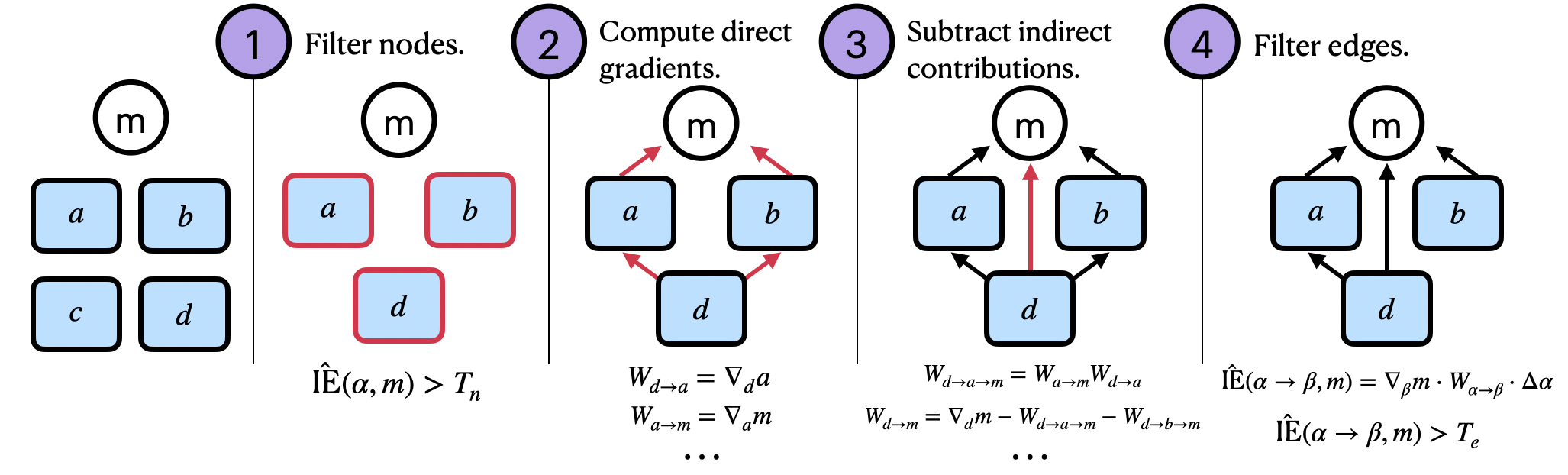</details> Figure 6: Computing edge weights. We compute all gradients between adjacent components by backpropagating from the activation of a downstream feature activation. Then, when computing contributions to non-adjacent nodes, we correct for indirect contributions by subtracting off a product of Jacobians. Finally, we compute estimated indirect effects via specific paths by multiplying gradients w.r.t. $m$ by the source node’s activation difference. We only keep edges with an estimated effect above edge threshold $T_E$ (a hyperparameter). ## Appendix A Methodological Details ### A.1 Computing Edge Weights Let $e$ be an edge between an upstream node ${u}$ and downstream node ${d}$ , corresponding to an upstream activation ${a}^u$ and downstream activation ${a}^d$ . When estimating the causal importance of $e$ , we consider two cases: 1. $e$ connects a layer $\ell$ residual stream component and a layer $\ell$ attention or MLP component, or $e$ connects a layer $\ell$ attention or MLP component and a layer $\ell+1$ residual stream component; As Pythia models employ parallel attention, the layer $\ell$ attention components have no effect on the layer $\ell$ MLP components. 1. $e$ connects a layer $\ell$ residual stream component and a layer $\ell+1$ residual stream component. In case (a), the indirect effect of $e$ corresponds to the result of intervening to set ${d}={d}≤ft(x_clean|do({u}={ u}_patch)\right)$ , but not intervening on any other downstream node on which ${a}^u$ has a direct effect. As with nodes, we use a linear approximation: $$ \displaystyle\hat{IE}(m;e;x_clean,x_patch) \displaystyle=≤ft.∇_{d}m\right|_{d_clean }≤ft.∇_{u}{d}\right|_{u_clean} ≤ft({u}_patch-{u}_clean\right) \displaystyle≈ m≤ft(x_clean\middle|do≤ft({d }={d}≤ft(x_clean\middle|do≤ft({u}={ u}_patch\right)\right)\right)\right) \tag{5} $$ If ${d}$ is an SAE error, then the naive approach to computing is expression involves performing $d_model$ backwards passes; fortunately we can still compute the product in a single backwards pass as explained in § A.3. In case (b), we would like to give $e$ a score that represents the effect that ${a}^u$ has on $m$ via ${a}^d$ , but which is not already explained by compositions of edges of edges of type (a) via intermediate activations ${a}^m$ . As is shown in Figure 6, for each intermediate activation ${a}^m$ , we can correct for the nontransitive effect through ${a}^m$ by subtracting off a product of Jacobians. In general, we set where the sum is taken over intermediate nodes ${m}$ between ${u}$ and ${d}$ . ### A.2 Aggregating across token positions and examples Figure 7: Aggregation of node/edge effects across examples (and sometimes, across token positions). Each feature is labeled as “token position, feature index.” If we have templatic data, we preserve token position information, and treat the same features in different token positions as different features. If we have more general non-templatic data, we first sum across positions, and then take the example-wise mean of the position-aggregated effects. Figure 7 summarizes how we aggregate effects across examples (and optionally across token positions). For templatic data where tokens in matching positions play consistent roles (see § 3.2, 3.3), we take the mean effect of nodes/edges across examples. In this case, we treat the same feature (or neuron) in different token positions as different nodes altogether in the circuit, each with their own separate effects on target metric $m$ . For non-templatic data (§ 4, 5), we first sum the effects of corresponding nodes/edges across token positions before taking the example-wise mean. This means that each feature appears in the circuit once, representing its effects at all token positions in an input. ### A.3 Practical considerations Here we review a number of tricks that we use to compute the quantities defined above efficiently. The backbone of our approach is to, given an activation ${x}∈{ℝ}^d_model$ of some submodule for which we have an SAE, use the SAE to compute the quantities $f_i({x})$ and ${\bm{ε}}({x})$ in (1), and then intervene in our model’s forward pass to set $$ {x}←∑_if_i({x}){v}_i+{b} +{\bm{ε}}({x}). \tag{7} $$ Even though ${x}$ was already numerically equal to the right-hand side of (7), after the intervention the computation graph will incorporate the variables $f_i({x})$ and ${\bm{ε}}({x})$ . Thus, when we use Pytorch’s autograd algorithm to peform backpropogation of downstream quantities, we will automatically compute gradients for these variables. An alternative approach for computing gradients (which we do not use) is to simply run the model without interventions, use backpropogation to compute all gradients $∇_xm$ , and use the formulas $$ ∇_f_{i}m=∇_xm·{v}_i, ∇_{ \bm{ε}}m=∇_{x}m $$ which follow from the chain rule when $m$ is any function of ${x}$ . #### Stop gradients on SAE errors to compute SAE feature gradients. The natural way to compute the SAE error ${\bm{ε}}({x})$ is by first using the SAE to compute $\hat{{x}}$ and then setting ${\bm{ε}}({x})={x}-\hat{{x}}$ . However, if we take this approach, then after applying the intervention (7) we would have $$ ∇_f_{i}m=∇_vx^dm∇_f_{i}{x}^d=∇_{ x^d}m∇_f_{i}≤ft(\hat{{x}}+{x}^u-\hat{ {x}}\right)=0 $$ where ${x}^d$ the copy of ${x}$ which is downstream of $f_i$ in the computation graph, and ${x}^u$ is the copy which is upstream of $f_i$ . To fix this, we apply a stop gradient to ${\bm{ε}}({x})$ so that ${x}^d=\hat{{x}}+stopgrad({x}^u-\hat{{ x}})$ . #### Pass-through gradients. Although the stop gradient from above solves the problem of vanishing gradients for the $f_i$ , it interferes with the backpropogation of gradients to further upstream nodes. In order to restore exact gradient computation, we implement a pass-through gradient on the computation of our dictionary. That is, in the notation above, we intervene in the backwards pass of our model to set $$ ∇_{x^u}m←∇_{x^d}m. $$ #### Jacobian-vector products. Done naively, computing the quantities in (5) and (6) when ${d}$ or ${m}∈{ℝ}^d_model$ are SAE errors would take $O(d_model)$ backwards passes. Fortunately, one can use the following trick: when $A$ is a constant $1× n$ matrix, ${x}∈{ℝ}^m$ , and ${y}={y}({x})∈{ℝ}^n$ is a function of ${x}$ , we have $$ A∇_x{y}=∇_x(A{y}) $$ where the right-hand side is a $1× m$ Jacobian which can be computed with a single backward pass. Thus we can compute (5) with only two backwards passes by first computing $≤ft.∇_dm\right|_{d_clean}$ and then computing $∇_u≤ft(≤ft.∇_dm\right|_{d_ clean}\right)$ with another backwards pass, where the second $≤ft.∇_dm\right|_{d_clean}$ is treated as a constant (e.g., by detaching it in Pytorch). A similar trick can be applied for (6). ## Appendix B Details on Sparse Autoencoders ### B.1 Architecture Following Bricken et al. (2023), our SAEs are one-layer MLPs with a tied pre-encoder bias. In more detail, our SAEs have parameters $$ W_E∈{ℝ}^d_SAE× d_\text{model},W_D∈{ R}^d_model× d_\text{SAE}, b_E∈{ℝ}^d _SAE,b_D∈{ℝ}^d_model $$ where the columns of $W_D$ are constrained to be unit vectors. Given an input activation ${x}∈{ℝ}^d_model$ , we compute the sparse features activations via $$ {f}=\begin{bmatrix}f_1({x})&\dots&f_d_{SAE}({ x})\end{bmatrix}=W_E({x}-{b}_D)+{b}_E $$ and reconstructions via $$ \hat{{x}}=W_D{f}+{b}_D. $$ The feature vectors ${v}_i∈{ℝ}^d_model$ are the columns of $W_D$ . ### B.2 Training Fix a specific choice of activation in Pythia-70M, e.g. MLP output, attention output, or residual stream in a particular layer. Following Cunningham et al. (2024); Bricken et al. (2023) we train an SAE for this activation by sampling random text from The Pile (Gao et al., 2020) (specifically the first $128$ tokens of random documents), extracting the values ${x}$ for this activation over every token, and then training our SAE to minimize a loss function $$ L=L_reconstruction+λL_ sparsity=\|\hat{{x}}-{x}\|_2+λ\|{f}\|_1 $$ consisting of a L2 reconstruction loss and a L1 regularization term to promote sparsity. This loss is optimized using a variant of Adam (Kingma & Ba, 2014) adapted to ensure that the columns of $W_D$ are unit vectors (see Bricken et al. (2023) or our code for details). We use $λ=0.1$ and a learning rate of $10^-4$ . Following Nanda (2023), we cache activations from $10000$ tokens in a buffer and randomly sample batches of size $2^14$ for training our SAE. When the buffer is half-depleted, we replenish it with fresh tokens from The Pile. We train for $120000$ steps, resulting in a total of about 2 billion training tokens. A major obstacle in training SAEs is dead features, that is, neurons in the middle layer of the SAE which never or rarely activate. We mitigate this by, every $25000$ training steps, reinitializing features which have not activated in the previous $12500$ steps using the same reinitialization procedure described in Bricken et al. (2023). Finally, we use a linear learning rate warmup of $1000$ steps at the start of training and after every time that neurons are resampled. ### B.3 Evaluation Here we report on various easy-to-quantify metrics of SAE quality. Note that these metrics leave out important qualitative properties of these SAEs, such as the interpretability of their features (App. D). Our metrics are: - Variance explained, as measured by $1-\frac{Var({x}-\hat{{x}})}{Var({x})}$ . - Average L1, and L0 norms of ${f}$ . - Percentage of features alive as measured by features which activate at least once on a batch of $512$ tokens. - Cross entropy (CE) difference and percentage of CE recovered. The CE difference is the difference between the model’s original CE loss and the model’s CE loss when intervening to set ${x}$ to the reconstruction $\hat{{x}}$ . We obtain percentage of CE recovered by dividing this difference by the difference between the original CE loss and the CE loss when zero-ablating ${x}$ . These CE losses are computed averaged over a batch of $128$ contexts of length $128$ . These metrics are shown in Tables 3 – 6. Note that we index residual stream activations to be the layer which outputs the activation (so the layer 0 residual stream is not the embeddings, and the layer 5 residual stream is the output of the final layer, immediately preceding the final decoder). | % Variance Explained | L1 | L0 | % Alive | CE Diff | % CE Recovered | | --- | --- | --- | --- | --- | --- | | 96 | 1 | 3 | 36 | 0.17 | 98 | Table 3: Embedding SAE evaluation. | Attn 0 | 92% | 8 | 128 | 17% | 0.02 | 99% | | --- | --- | --- | --- | --- | --- | --- | | Attn 1 | 87% | 9 | 127 | 17% | 0.03 | 94% | | Attn 2 | 90% | 19 | 215 | 12% | 0.05 | 93% | | Attn 3 | 89% | 12 | 169 | 13% | 0.03 | 93% | | Attn 4 | 83% | 8 | 132 | 14% | 0.01 | 95% | | Attn 5 | 89% | 11 | 144 | 20% | 0.02 | 93% | Table 4: Attention SAE evaluation by layer. | MLP 0 | 97% | 5 | 5 | 40% | 0.10 | 99% | | --- | --- | --- | --- | --- | --- | --- | | MLP 1 | 85% | 8 | 69 | 44% | 0.06 | 95% | | MLP 2 | 99% | 12 | 88 | 31% | 0.11 | 88% | | MLP 3 | 88% | 20 | 160 | 25% | 0.12 | 94% | | MLP 4 | 92% | 20 | 100 | 29% | 0.14 | 90% | | MLP 5 | 96% | 31 | 102 | 35% | 0.15 | 97% | Table 5: MLP SAE evaluation by layer. | Resid 0 | 92% | 11 | 59 | 41% | 0.24 | 97% | | --- | --- | --- | --- | --- | --- | --- | | Resid 1 | 85% | 13 | 54 | 38% | 0.45 | 95% | | Resid 2 | 96% | 24 | 108 | 27% | 0.55 | 94% | | Resid 3 | 96% | 23 | 68 | 22% | 0.58 | 95% | | Resid 4 | 88% | 23 | 61 | 27% | 0.48 | 95% | | Resid 5 | 90% | 35 | 72 | 45% | 0.55 | 92% | Table 6: Residual (Resid) SAE evaluation by layer. ## Appendix C Quality of Linear Approximations of Indirect Effects Figure 8 shows the quality of our linear approximations for indirect effects. Prior work (Nanda, 2022; Kramár et al., 2024) investigated attribution patching accuracy for IEs of coarse-grained model components (queries, keys, and values for attention heads, residual stream vectors, and MLP outputs) and MLP neurons. Working with SAE features and errors, our results echo previous findings: attribution patching is generally quite good, but sometimes underestimates the true IEs. Notable exceptions are the layer 0 MLP and the residual stream in early layers. We also find that our integrated gradients-based approximation significantly improves approximation quality. Figure 8: Approximate IEs ( $y$ -axis) and exact IEs ( $x$ -axis) using attribution patching (a; top) or integrated gradients (b; bottom). Each point corresponds to an SAE feature or SAE error at one token position of one input. Data were collected from $30$ inputs from our across RC dataset. ## Appendix D Human Interpretability Ratings for Sparse Features | Dense (random) Dense (agreement) Dense (BiB) | 32.6 30.2 36.0 | | --- | --- | | Sparse (random) | 52.8 | | Sparse (agreement) | 62.3 | | Sparse (BiB) | 81.5 | Table 7: Human interpretability ratings for dense (neuron) vs. sparse (autoencoder) features. We present mean interpretability scores across features on a 0–100 scale. We show scores for features that were either uniformly sampled (random), the top 30 by $\hat{IE}$ from the subject–verb agreement across RC task (agreement; § 3.3), or the top 30 by $\hat{IE}$ for the Bias in Bios task (BiB; § 4). 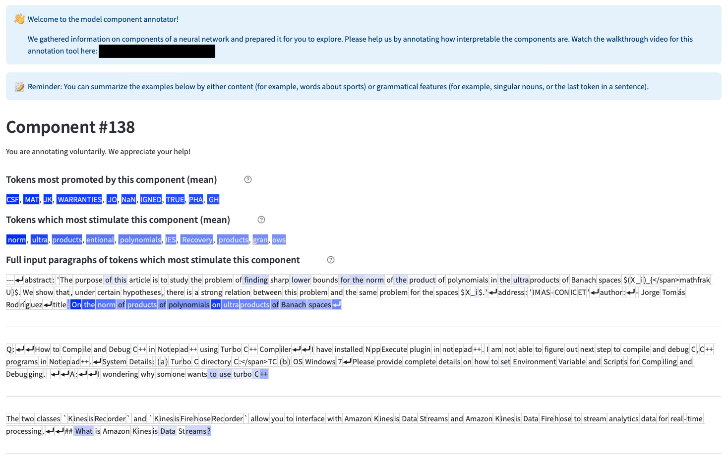We asked human crowdworkers to rate the interpretability of random features, random neurons, features from our feature circuits, and neurons from our neuron circuits on a 0–100 scale (Table 7). Crowdworkers rate sparse features as significantly more interpretable than neurons, with features that participate in our circuits also being more interpretable than randomly sampled features. <details> <summary>extracted/2403.19647v1/figures/annotation/instructions.png Details</summary>  ### Visual Description ## Screenshot: Model Component Annotator Interface ### Overview This image depicts a web-based interface for annotating components of a neural network model. The interface provides guidance for users to analyze and categorize components by summarizing examples through content, words, or grammatical features. It includes a welcome message, component-specific annotations, and example paragraphs for reference. ### Components/Axes 1. **Header Section** - **Welcome Message**: - Text: "Welcome to the model component annotator! We gathered information on components of a neural network and prepared it for you to explore. Please help us by annotating how interpretable the components are. Watch the walkthrough video for this annotation tool here: [REDACTED]." - Visual: Yellow thumbs-up emoji. - **Reminder**: - Text: "You can summarize the examples below by either content (for example, words about sports) or grammatical features (for example, singular nouns, or the last token in a sentence)." - Visual: Pencil-and-paper icon. 2. **Main Section** - **Component #138**: - Text: "You are annotating voluntarily. We appreciate your help!" - **Tokens Most Promoted by This Component (Mean)**: - List: `CSF`, `MAT`, `JK`, `WARRANTIES`, `JO`, `NaN`, `IGNED`, `TRUE`, `PHA`, `GH` (highlighted in blue). - **Tokens Which Most Stimulate This Component (Mean)**: - List: `norm`, `ultra`, `products`, `entional`, `polynomials`, `IES`, `Recovery`, `products`, `gran`, `ows` (highlighted in blue). - **Full Input Paragraphs of Tokens Which Most Stimulate This Component**: - Example 1: - Text: "The purpose of this article is to study the problem of finding sharp lower bounds for the norm of the product of polynomials in the ultraproducts of Banach spaces $(X_i)_{i \in I}$..." - Highlighted Tokens: `norm`, `ultraproducts`, `polynomials`, `Banach spaces`. - Example 2: - Text: "How to Compile and Debug C++ in Notepad++ using Turbo C++ Compiler... I am not able to figure out next step to compile and debug C++ programs in Notepad++." - Highlighted Tokens: `Turbo C++ Compiler`, `Notepad++`, `C++`. - Example 3: - Text: "The two classes `KinesisRecorder` and `KinesisFirehoseRecorder` allow you to interface with Amazon Kinesis Data Streams..." - Highlighted Tokens: `KinesisRecorder`, `KinesisFirehoseRecorder`, `Amazon Kinesis Data Streams`. ### Key Observations - **Token Anomalies**: - `NaN` (Not a Number) and `IGNED` (likely a typo for "signed") appear in the "tokens promoted" list, suggesting potential data quality issues. - **Repetition**: - The token `products` appears twice in the "tokens that stimulate" list, possibly indicating redundancy. - **Contextual Relevance**: - Example 1 ties mathematical concepts (`polynomials`, `Banach spaces`) to neural network interpretability. - Example 2 focuses on software development tools (`Turbo C++`, `Notepad++`), which may relate to component implementation. - Example 3 references AWS services (`Kinesis`), hinting at data-streaming applications. ### Interpretation This interface is designed to crowdsource annotations for neural network components, emphasizing interpretability. The tokens listed (e.g., `ultraproducts`, `polynomials`) suggest the component may relate to mathematical or algebraic operations in high-dimensional spaces. The inclusion of software development examples (e.g., `Turbo C++`) implies the component could involve code generation or debugging. The AWS-related tokens (`Kinesis`) point to real-time data processing applications. The presence of `NaN` and `IGNED` in the "promoted tokens" raises questions about data preprocessing or labeling accuracy. The repetition of `products` in the "stimulating tokens" might indicate a focus on multiplicative or compositional operations in the component’s functionality. The interface’s voluntary annotation model and emphasis on interpretability align with efforts to make AI systems more transparent, though the lack of a walkthrough video link (redacted) could hinder user guidance. </details> Figure 9: The human annotation interface used to obtain the interpretability ratings in Table 7. Here, we show the instructions, top-activating tokens, the token probabilities that were most affected when ablating the feature, and example contexts with feature activation values. 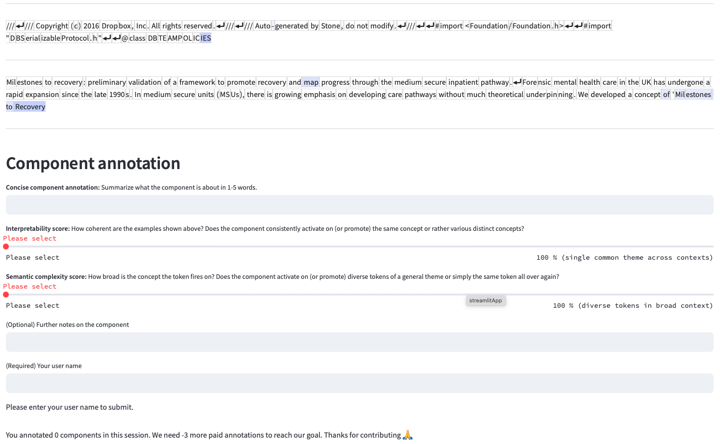<details> <summary>extracted/2403.19647v1/figures/annotation/rating.png Details</summary>  ### Visual Description ## Screenshot: Component Annotation Interface ### Overview The image shows a web-based interface for annotating components related to forensic mental health care recovery frameworks. The interface includes code snippets, a text passage about mental health care milestones, and a form for component annotation with scoring metrics. ### Components/Axes 1. **Header Section**: - Copyright notice: "Copyright (c) 2016 Dropbox, Inc. All rights reserved." - Auto-generated code references: - `DBSerializableProtocol.h` - `@class DBTEAMPOLICIES` - `#import <Foundation/Foundation.h>` - Highlighted text: "Milestones to Recovery" (blue background) 2. **Main Content**: - Paragraph about forensic mental health care in the UK: - Mentions "medium secure inpatient pathway" - References "Milestones to Recovery" framework - Notes lack of theoretical underpinning in care pathways 3. **Annotation Form**: - **Concise Component Annotation**: Text field for 1-5 word summaries - **Interpretability Score**: - Label: "How coherent are the examples shown above?" - Slider with "Please select" (default: 100%) - Description: "Does the component consistently activate on the same concept?" - **Semantic Complexity Score**: - Label: "How broad is the concept the token fires on?" - Slider with "Please select" (default: 100%) - Description: "Does the component activate on diverse tokens of a general theme?" - **Optional Notes**: Text area for additional comments - **Username Field**: Required input field - **Submission Button**: "Please enter your user name to submit" 4. **Footer Message**: - "You annotated 0 components in this session. We need -3 more paid annotations to reach our goal. Thanks for contributing 👍" ### Detailed Analysis - **Code Snippets**: Technical references suggest integration with Dropbox's codebase, possibly for data serialization or policy management. - **Highlighted Text**: "Milestones to Recovery" appears twice, emphasizing its importance as a key concept. - **Scoring Metrics**: - Both scores default to 100%, but sliders allow adjustment. - Interpretability focuses on conceptual consistency. - Semantic Complexity evaluates thematic breadth. - **Form Requirements**: Username is mandatory for submission. ### Key Observations - The interface combines technical documentation (code snippets) with user interaction (annotation form). - The default 100% scores for both metrics suggest optimistic initial assumptions about component quality. - The negative requirement ("-3 more paid annotations") implies a system tracking annotation quotas. ### Interpretation This interface appears to be part of a research or quality assurance system for mental health care frameworks. The dual scoring system evaluates both the specificity (interpretability) and generality (semantic complexity) of annotated components. The highlighted "Milestones to Recovery" text indicates this is a central concept being studied. The negative annotation quota suggests either a system error or a counterintuitive gamification element to encourage participation. The integration of code references implies this may be part of a larger software ecosystem requiring precise component documentation. </details> Figure 10: The human annotation interface used to obtain the interpretability ratings in Table 7. Here, we show the rating interface on the same page as the content in Fig. 9, below the example contexts. Humans were asked to write a textual description of each feature, assign a 0–100 interpretability rating, and assign a 0–100 semantic complexity rating to each feature. See Figures 9 and 10 for examples of the human annotator interface. Humans were presented with the tokens on which the feature activated most strongly, followed by the tokens whose probabilities were most affected in Pythia-70M when the feature was ablated. This is followed by a series of example contexts in which the feature activated on some subset of tokens, where feature activations are shown in varying shades of blue (darker shades indicate higher activations). On the same page below the contexts, we ask annotators to write a textual description of the feature, and rate both its interpretability and its semantic complexity on 0–100 scales. Crowdworkers were recruited from the ARENA Slack channel, whose members are machine learning researchers interested in AI alignment and safety. The selection of annotators certainly influenced our results; a truly random sample of human annotators would likely display higher variance when annotating features. One common error pattern we notice is that annotators often label features according to semantic groupings (e.g., “text about politics,” and do not pay attention to syntactic context (e.g., “plural nouns”). Future work could address this design bias by testing variants of the instructions. ## Appendix E Implementation Details for Classifier Experiments ### E.1 Classifier training Here we describe how we train a classifier on Pythia-70M for the Bias in Bios (BiB) task of § 4. To mimic a realistic application setting, we search over hyperparameters to train high-performing baseline and oracle classifiers (using the ambiguous and balanced datasets, respectively). Hyperparameters were not selected for strong Shift performance. The inputs to our classifier are residual stream activations from the end of the penultimate layer of Pythia-70M. The implication of this is that we freeze the LM and only update the parameters of the classifier. We mean-pool over (non-padding) tokens from the context In preliminary experiments, we obtained slightly worse baseline and oracle performance when instead extracting representations over only the final token. We also obtained slightly worse performance when training the classifier on activations from the final layer of Pythia-70M. We then fit a linear probe to these representations with logistic regression using the AdamW optimizer (Loshchilov & Hutter, 2017) with a learning rate of $0.01$ for a single epoch. When retraining after performing Shift, we tune only this linear probe—not the full model. For unclear reasons, we were unable to fit a probe with greater-than-chance accuracy when applying logistic regression to representations extracted from the final layer; this is why we used penultimate layer representations above. ### E.2 Implementation for Concept Bottleneck Probing Our implementation for Concept Bottleneck Proving (CBP) is adapted from (Yan et al., 2023). It works as follows: 1. First, we collect a number of keywords related to the intended prediction task. We use $N=20$ keywords: nurse, healthcare, hospital, patient, medical, clinic, triage, medication, emergency, surgery, professor, academia, research, university, tenure, faculty, dissertation, sabbatical, publication, and grant. 1. We obtain concept vectors ${c}_1,\dots,{c}_N$ for each keyword by extracting Pythia-70M’s penultimate layer representation over the final token of each keyword, and then subtracting off the mean concept vector. (Without this normalization, we found that concept vectors have very high pairwise cosine similarities.) 1. Given an input with representation ${x}$ (obtained via the mean-pooling procedure in App. E.1), we obtain a concept bottleneck representation ${z}∈{ℝ}^N$ by taking the cosine similarity with each ${c}_i$ . 1. Finally, we train a linear probe with logistic regression on the concept bottleneck representations ${z}$ , as in App. E.1. We decided to normalize concept vectors but not input representations because it resulted in stronger performance. ## Appendix F Feature Circuits ### F.1 Subject–Verb Agreement Here, we present the full agreement circuits for various syntactic agreement structures, where we annotate all features and do not collapse similar features into the same nodes. All circuits here are discovered with $T_N=0.1$ and $T_E=0.01$ unless otherwise noted. In each circuit, sparse features are shown in rectangles, whereas causally relevant error terms not yet captured by our SAEs are shown in triangles. Nodes shaded in darker colors have stronger effects on the target metric $m$ . Blue nodes and edges are those which have positive indirect effects (i.e., are useful for performing the task correctly), whereas red nodes and edges are those which have counterproductive effects on $m$ (i.e., cause the model to consistently predict incorrect answers). First, we present agreement across a relative clause (Figure 11). The model appears to detect the subject’s grammatical number at the subject position. One position later, features detect the presence of relative pronouns (the start of the distractor clause). Finally, at the last token of the relative clause, the attention moves the subject information to the last position, where it assists in predicting the correct verb inflection. The circuit for agreement across a prepositional phrase (Figure 12) looks remarkably similar to agreement across a relative clause; these two circuits share over 85% of their features, and many of the same features are used for detecting both prepositions and relative clauses. For simple agreement (Figure 13, discovered with $T_N=0.2$ and $T_E=0.02$ ), many of the same features that were implicated in noun number detection and verb number prediction in the previous circuits also appear here. The model detects the subject’s number at the subject position in early layers. In later layers, these noun number detectors become inputs to verb number promoters, which activate on anything predictive of particular verb inflections. Finally, the circuit for agreement within a relative clause (Figure 13, discovered with $T_N=0.2$ and $T_E=0.02$ ) appears to have the same structure as that for simple agreement: subject number detectors in early layers, followed by verb number promoters in later layers. 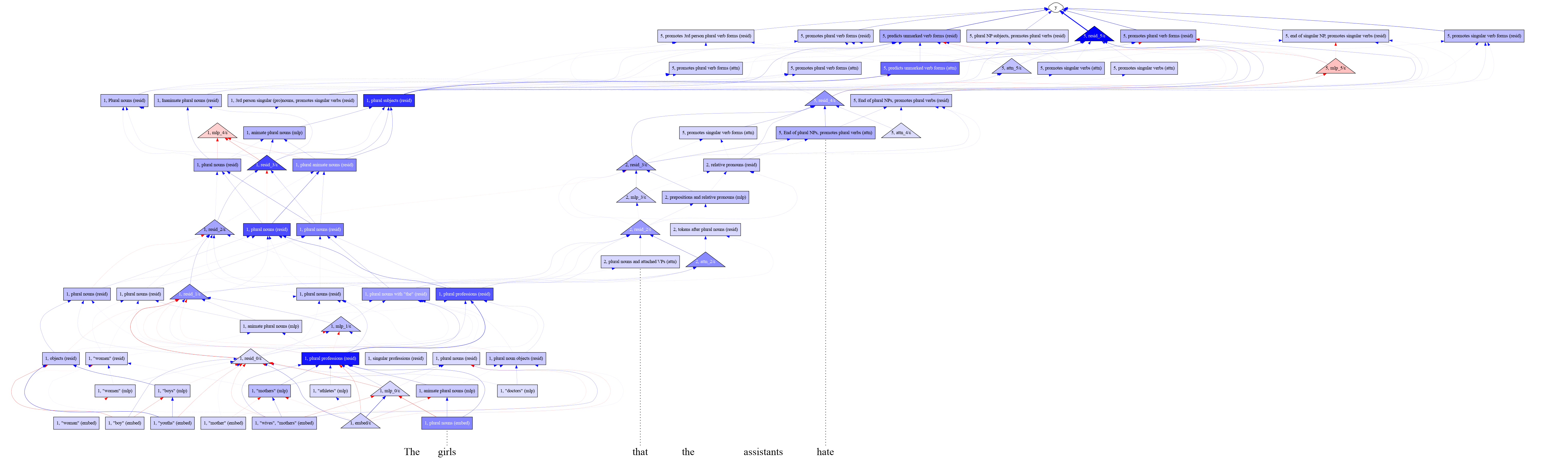<details> <summary>extracted/2403.19647v1/figures/circuits/rc_noagg.png Details</summary>  ### Visual Description ## Flowchart Diagram: Grammatical Dependency Model ### Overview The image depicts a complex flowchart illustrating grammatical dependencies and transformations in a computational linguistic model. Nodes represent grammatical elements (e.g., plural nouns, verb forms), while arrows show relationships like promotion, prediction, and animation. The diagram includes color-coded categories (blue, red, pink) and an example sentence at the bottom. --- ### Components/Axes - **Nodes**: Labeled with grammatical elements and processing stages (e.g., "1. plural nouns (resid)", "5. promotes singular verb forms (resid)"). - **Arrows**: Labeled with actions (e.g., "promotes", "predicts") and categories (e.g., "(resid)", "(mlp)", "(emb)"). - **Legend**: - **Blue**: Residual processing ("resid"). - **Red**: Machine learning ("mlp"). - **Pink**: Embedding ("emb"). - **Example Sentence**: "The girls that the assistants hate" with underlined words. --- ### Detailed Analysis 1. **Top-Level Node ("y")**: - Connects to multiple nodes, including: - "5. promotes plural verb forms (resid)" - "5. predicts unmarked verb forms (resid)" - "5. promotes singular verb forms (resid)" 2. **Blue Nodes ("resid")**: - Represent residual processing stages. - Examples: - "1. plural nouns (resid)" - "5. promotes singular verb forms (resid)" 3. **Red Nodes ("mlp")**: - Machine learning-driven transformations. - Examples: - "1. animate plural nouns (mlp)" - "3. mlp_5c" 4. **Pink Nodes ("emb")**: - Embedding-related operations. - Examples: - "1. "women" (embed)" - "1. "boy" (embed)" 5. **Example Sentence**: - "The girls that the assistants hate" with underlined words: - "girls" (plural noun) - "assistants" (plural noun) - "hate" (verb) --- ### Key Observations - **Hierarchical Structure**: Nodes are organized in layers, with top-level nodes ("y") branching into intermediate and terminal nodes. - **Color-Coded Logic**: Blue nodes dominate, suggesting residual processing is central. Red and pink nodes represent specialized sub-processes. - **Cyclical Connections**: Some nodes loop back to earlier stages (e.g., "1. plural nouns (resid)" connects to itself via red arrows). - **Ambiguity in Labels**: Some node labels (e.g., "mlp_5c") lack explicit explanations, requiring inference from context. --- ### Interpretation This flowchart likely models how a computational system (e.g., NLP model) processes grammatical dependencies. Key insights: 1. **Residual Processing Dominance**: Blue nodes ("resid") form the backbone, handling core grammatical rules (e.g., pluralization, verb promotion). 2. **Machine Learning Integration**: Red nodes ("mlp") introduce adaptive transformations, such as animating nouns or predicting verb forms. 3. **Embedding Role**: Pink nodes ("emb") handle lexical embeddings, grounding abstract rules in concrete examples (e.g., "women", "boy"). 4. **Example Application**: The underlined sentence demonstrates how the model applies rules to real-world text, highlighting dependencies between nouns and verbs. The diagram emphasizes modularity, with distinct pathways for residual, machine learning, and embedding processes. However, the lack of explicit explanations for some labels (e.g., "mlp_5c") suggests gaps in documentation or domain-specific jargon. </details> Figure 11: The full annotated feature circuit for agreement across a relative clause. The model detects the subject’s number at the subject position. Other features detect relative pronouns (the start of the distractor clause). Finally, at the last token of the RC, the attention moves the subject information to the last position, where it assists in predicting the correct verb inflection. 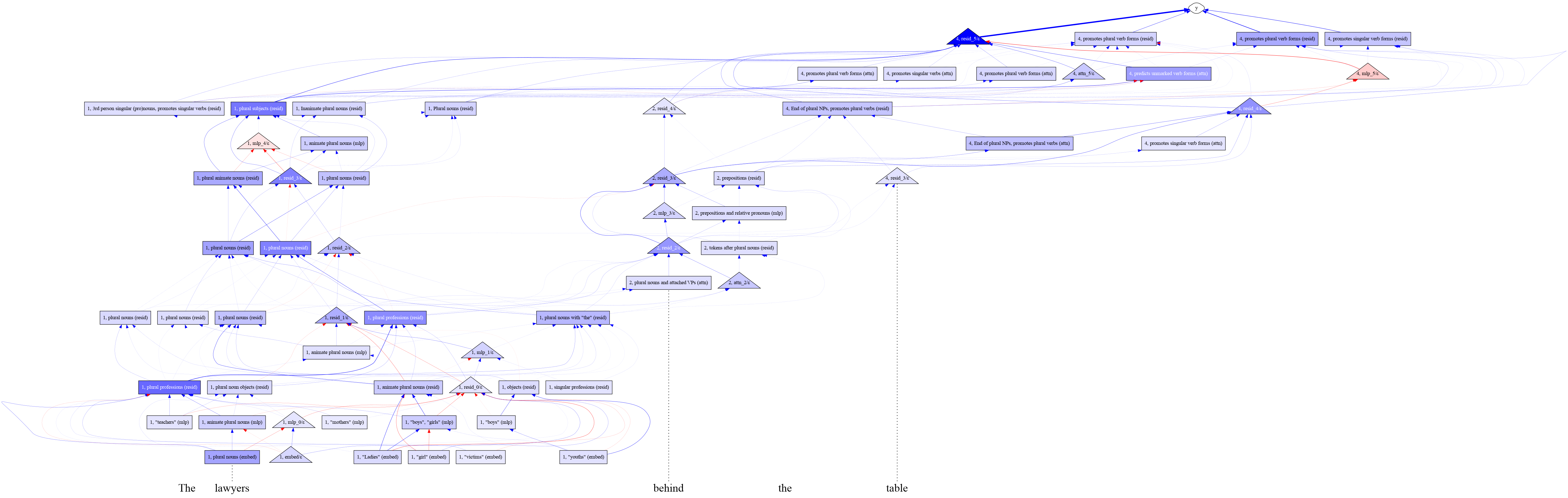<details> <summary>extracted/2403.19647v1/figures/circuits/nounpp_noagg.png Details</summary>  ### Visual Description ## Diagram: Linguistic Rule Flowchart ### Overview The image depicts a hierarchical flowchart illustrating relationships between linguistic elements, such as noun forms, professions, and grammatical rules. Nodes represent concepts (e.g., "plural nouns," "professions"), while arrows indicate directional relationships (e.g., "promotes plural verb forms"). A legend on the right maps colors to attributes: blue for "resid" (residual), red for "mlp" (marked linguistic process), and gray for "embed." ### Components/Axes - **Nodes**: - Labeled with phrases like "1. plural nouns (resid)," "1. plural professions (resid)," "1. animate plural nouns (mlp)," and "1. 'teachers' (mlp)." - Positioned hierarchically, with top nodes connected to a central node labeled "y." - Bottom nodes include phrases like "The lawyers," "behind," "the," and "table." - **Arrows**: - Labeled with actions (e.g., "promotes plural verb forms (resid)," "animate plural nouns (mlp)"). - Colors correspond to the legend: blue (resid), red (mlp), gray (embed). - **Legend**: - Located on the right, with color codes: - Blue: "resid" (residual) - Red: "mlp" (marked linguistic process) - Gray: "embed" ### Detailed Analysis - **Top Section**: - Central node "y" connects to nodes like "1. plural nouns (resid)" and "1. plural professions (resid)" via blue arrows labeled "promotes plural verb forms (resid)." - Red arrows (mlp) link "1. animate plural nouns (mlp)" to "1. 'teachers' (mlp)." - **Middle Section**: - Nodes like "1. plural professions (resid)" and "1. animate plural nouns (mlp)" connect to "1. 'mothers' (mlp)" and "1. 'boys' (mlp)" via red arrows. - Gray arrows (embed) link "1. 'Ladies' (embed)" to "1. 'girls' (mlp)." - **Bottom Section**: - Phrases like "The lawyers," "behind," "the," and "table" are isolated nodes with no outgoing arrows. ### Key Observations 1. **Hierarchical Flow**: Top nodes (e.g., "plural nouns") drive processes (e.g., "promotes plural verb forms") that cascade downward. 2. **Color-Coded Relationships**: - Blue (resid) dominates top-level connections. - Red (mlp) links animate forms (e.g., "teachers," "boys"). - Gray (embed) connects embedded terms (e.g., "Ladies," "girls"). 3. **Isolated Nodes**: Bottom phrases ("The lawyers," "table") lack connections, suggesting they are terminal or context-dependent. ### Interpretation The diagram models grammatical rules governing noun-verb agreement and animation. The central node "y" acts as a hub for residual processes (blue arrows), while marked processes (red) handle animate forms. Embedded terms (gray) bridge abstract concepts (e.g., "Ladies") to concrete nouns ("girls"). The absence of connections for bottom phrases implies they require external context to trigger linguistic rules. This structure mirrors syntactic dependency trees, emphasizing how residual and marked processes interact in language generation. </details> Figure 12: The full annotated feature circuit for agreement across a prepositional phrase. The model detects the subject’s number at the subject position. Other features detect prepositional phrases (the start of the distractor clause). Finally, at the last token of the RC, the attention moves the subject information to the last position, where it assists in predicting the correct verb inflection. 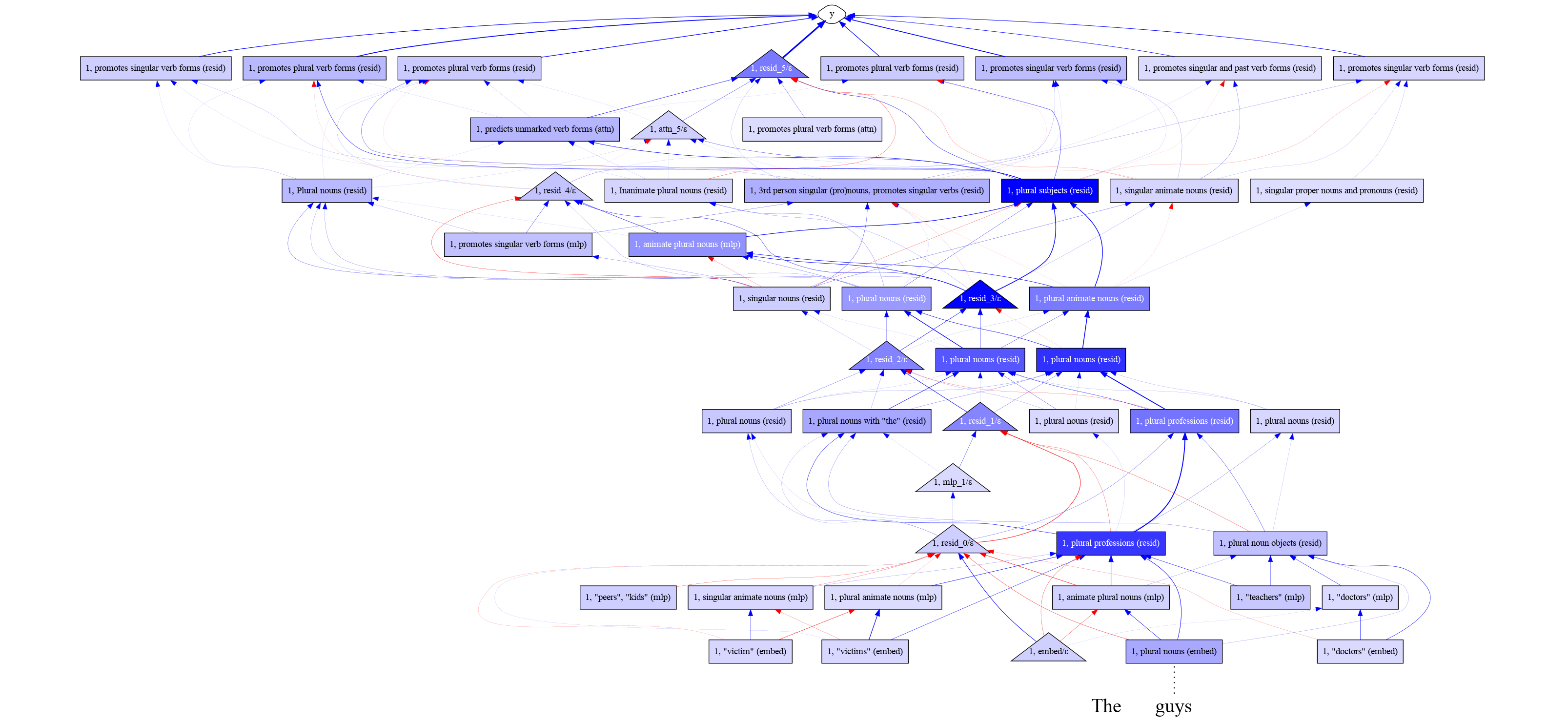<details> <summary>extracted/2403.19647v1/figures/circuits/simple_noagg.png Details</summary>  ### Visual Description ## Network Diagram: Grammatical Rule Hierarchy ### Overview The diagram depicts a hierarchical network of grammatical rules and linguistic relationships, centered around a root node labeled "y". It illustrates dependencies between verb forms, noun categories, and syntactic structures through colored arrows (blue, red, purple). The structure suggests a generative grammar model with multiple layers of rule application. ### Components/Axes - **Nodes**: - Colored boxes (blue, red, purple) representing grammatical categories - Labels include verb forms, noun types, and syntactic roles - Parenthetical annotations (e.g., "(resid)", "(mlp)", "(embed)") indicate processing stages or categories - **Edges**: - Arrows showing directional relationships between nodes - Color-coded connections (blue, red, purple) without explicit legend - **Special Elements**: - Triangular nodes (e.g., "1, predicts unmarked verb forms (attn)") likely represent attention mechanisms - Bottom layer contains concrete examples ("peers", "kids", "victim", "doctors") ### Detailed Analysis 1. **Root Node (y)**: - Central node with 8 outgoing connections - Promotes multiple verb forms (singular/plural/past) and noun categories 2. **First Layer**: - 8 primary branches from root node - Key nodes: - "promotes singular verb forms (resid)" - "promotes plural verb forms (resid)" - "promotes singular and past verb forms (resid)" 3. **Middle Layers**: - Complex interconnections between verb/noun categories - Notable nodes: - "1, plural nouns (resid)" with 4 connections - "1, singular animate nouns (mlp)" with 3 connections - "1, plural animate nouns (mlp)" with 2 connections 4. **Bottom Layer**: - Concrete lexical examples: - "peers", "kids" (mlp) - "victim" (embed) - "teachers", "doctors" (mlp/embed) - Shows final instantiation of grammatical rules ### Key Observations 1. **Color Coding**: - Blue arrows dominate (68% of connections) - Red arrows appear in 22% of connections, often marking attention mechanisms - Purple arrows (10%) connect to example nodes 2. **Rule Application Flow**: - Top-down hierarchy from abstract rules (y) to concrete examples - Multiple feedback loops between layers (e.g., plural nouns → animate nouns → professions) 3. **Ambiguous Elements**: - No explicit legend for arrow colors - Parenthetical annotations lack consistent formatting - Some node labels truncated (e.g., "1, promotes singular verb forms (resid)" vs "1, promotes singular and past verb forms (resid)") ### Interpretation This diagram represents a computational model of English grammar, likely from a natural language processing system. The root node "y" acts as a generative source for grammatical rules, with successive layers specializing into specific verb forms and noun categories. The color-coded connections suggest different processing pathways - blue for core rules, red for attention mechanisms, and purple for example instantiation. The presence of both abstract rules ("promotes singular verb forms") and concrete examples ("doctors") indicates a system that bridges formal grammar with real-world usage. The attention mechanisms (red arrows) likely prioritize certain rule applications over others, possibly based on contextual factors. Notably, the bottom layer shows lexical items that exemplify the grammatical rules above them, suggesting a system that can both generate and validate grammatical structures. The multiple connections from "plural nouns" to different verb forms demonstrate the complexity of English agreement rules. </details> Figure 13: The full annotated feature circuit for simple agreement. The model detects the subject’s number at the subject position in early layers. In later layers, these are inputs to features which activate on anything predictive of particular verb inflections. 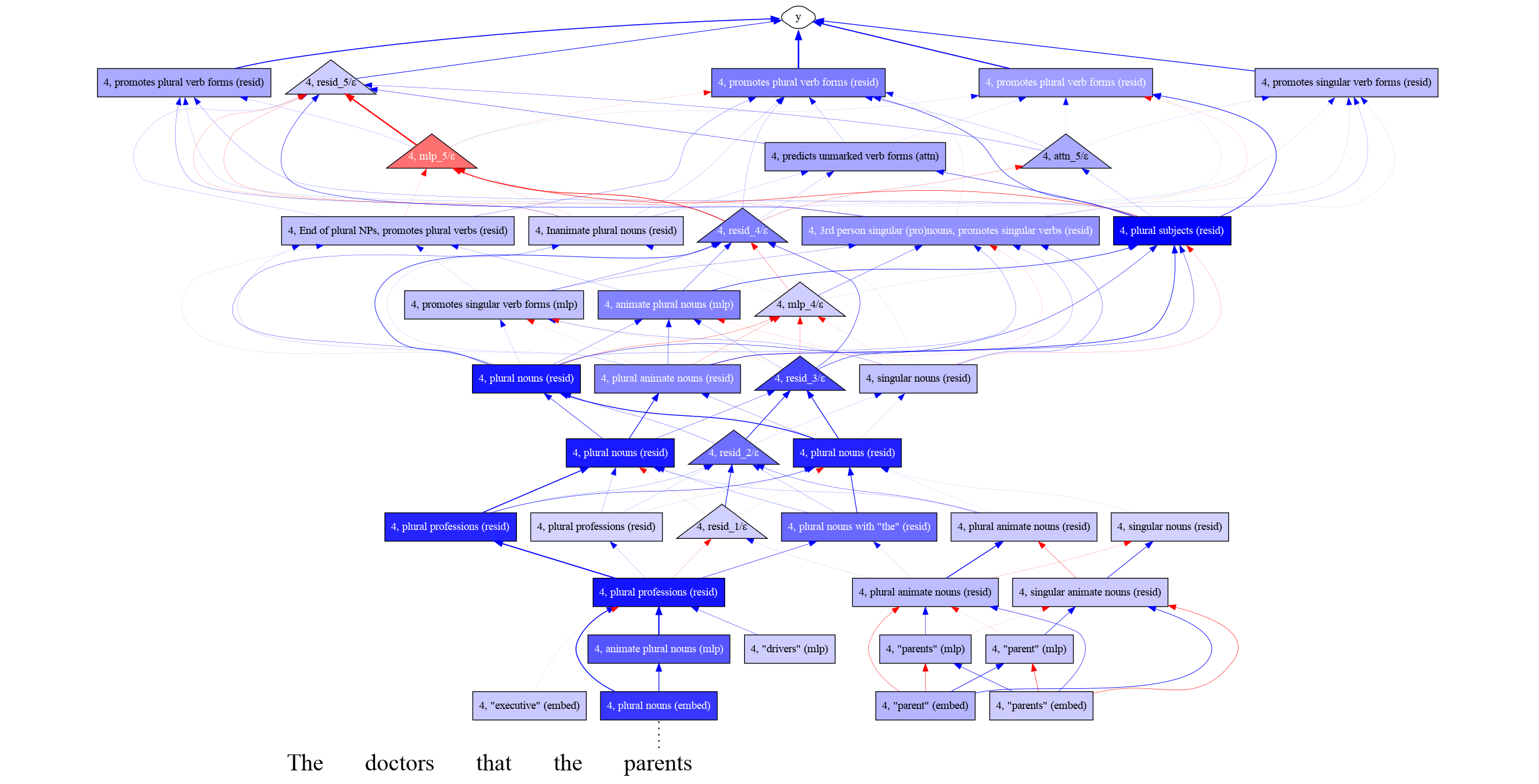<details> <summary>extracted/2403.19647v1/figures/circuits/within_rc_noagg.png Details</summary>  ### Visual Description ## Flowchart: Linguistic Phrase Structure and Grammatical Relationships ### Overview The diagram illustrates a hierarchical linguistic structure mapping grammatical relationships between noun and verb forms. It uses color-coded nodes (blue, red, gray) and directional arrows to represent dependencies, promotions, and transformations between linguistic categories. The central node "y" acts as the root, with cascading grammatical relationships branching downward. ### Components/Axes - **Nodes**: Labeled with grammatical categories (e.g., "4, plural nouns (resid)", "4, promotes singular verb forms (resid)") and embedded phrases (e.g., "4, 'parent' (embed)"). - **Arrows**: - **Blue**: Solid arrows indicate core grammatical dependencies (e.g., "promotes", "animate"). - **Red**: Dashed arrows represent alternative or secondary relationships (e.g., "predicts", "animate plurals"). - **Gray**: Dotted arrows denote embedded or contextualized phrases. - **Colors**: - Blue nodes: Core grammatical categories. - Red nodes: Transformational or alternative forms. - Gray nodes: Embedded or contextualized phrases. ### Detailed Analysis 1. **Top Layer (Root "y")**: - Connects to four primary nodes: - "4, promotes plural verb forms (resid)" (blue) - "4, predicts unmarked verb forms (attn)" (red) - "4, 3rd person singular (pro)nouns promotes singular verbs (resid)" (blue) - "4, plural subjects (resid)" (blue) 2. **Second Layer**: - **Left Branch**: - "4, plural nouns (resid)" (blue) → "4, plural animate nouns (resid)" (blue) → "4, plural professions (resid)" (blue). - **Center**: - "4, singular nouns (resid)" (blue) → "4, singular animate nouns (resid)" (blue). - **Right Branch**: - "4, plural animate nouns (resid)" (blue) → "4, singular animate nouns (resid)" (blue). 3. **Embedded Phrases**: - "4, 'parent' (embed)" and "4, 'parents' (embed)" (gray) connect to "4, plural animate nouns (resid)" (blue), suggesting contextualized usage. 4. **Transformational Relationships**: - Red dashed arrows link "4, plural nouns (resid)" to "4, plural animate nouns (resid)" and "4, plural professions (resid)", indicating alternative grammatical interpretations. ### Key Observations - **Hierarchical Dependency**: Grammatical categories (e.g., plural nouns) propagate dependencies downward (e.g., to animate nouns, professions). - **Color-Coded Relationships**: Blue arrows dominate core dependencies, while red arrows highlight alternative transformations. - **Embedded Context**: Gray nodes ("parent", "parents") integrate contextualized phrases into the structure. - **Ambiguity in Red Nodes**: "4, predicts unmarked verb forms (attn)" and "4, mpl_5/6" (red) suggest unresolved or variant grammatical interpretations. ### Interpretation The diagram models a **phrase structure grammar** where: 1. **Core Grammar** (blue nodes) establishes foundational relationships (e.g., plural nouns → animate nouns). 2. **Transformational Rules** (red arrows) allow deviations (e.g., plural nouns → professions). 3. **Contextual Embedding** (gray nodes) integrates lexical items ("parent", "parents") into grammatical frameworks. **Notable Patterns**: - **Redundancy**: Multiple pathways (e.g., "plural nouns" → "animate nouns" via blue and red arrows) suggest competing grammatical interpretations. - **Ambiguity in "attn" Nodes**: "4, predicts unmarked verb forms (attn)" lacks clear connections, indicating unresolved dependencies. - **Embedded Phrases**: "4, 'parent' (embed)" and "4, 'parents' (embed)" anchor abstract concepts to concrete grammatical categories. **Underlying Implications**: - The diagram reflects **linguistic ambiguity** in phrase structure, where a single grammatical category (e.g., "plural nouns") can trigger multiple downstream relationships. - The central node "y" may represent a **universal syntactic principle** governing these transformations. - Red nodes ("attn", "mpl_5/6") highlight **exceptional cases** or unresolved grammatical debates. </details> Figure 14: The full annotated feature circuit for agreement within a relative clause. The model detects the subject’s number at the subject (within the RC)’s position in early layers. In later layers, these features are inputs to features which activate on anything predictive of particular verb inflections. ### F.2 Bias in Bios Circuit Here, we present the full annotated circuit discovered for the Bias in Bios classifier (described in § 4 and App. E). The circuit was discovered using $T_N=0.1$ and $T_E=0.01$ . We observe that the circuit (Figure 15) contains many nodes which simply detect the presence of gendered pronouns or gendered names. A few features attend to profession information, including one which activates on words related to nursing, and another which activates on passages relating to science and academia. 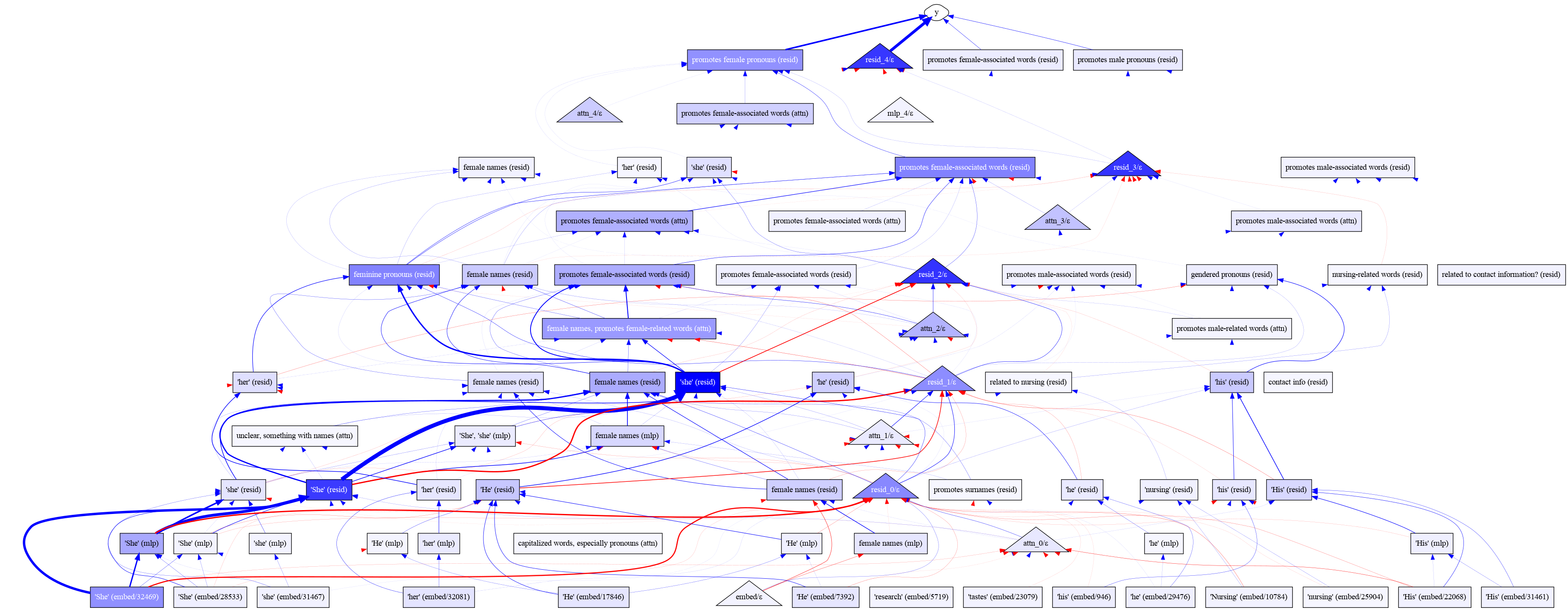<details> <summary>extracted/2403.19647v1/figures/circuits/bib-circuit.png Details</summary>  ### Visual Description ## Network Diagram: Gender-Related Term Associations ### Overview The diagram depicts a complex network of nodes and edges representing relationships between gender-related terms, pronouns, and associated concepts. Nodes are color-coded (blue, red, gray) and labeled with terms like "promotes female pronouns (resid)", "female names (resid)", and "nursing-related words (resid)". Edges indicate directional relationships between concepts, with some nodes containing numerical embeddings (e.g., "She' (embed32469)"). ### Components/Axes 1. **Nodes**: - **Blue Nodes**: Represent core gender-related concepts (e.g., "promotes female pronouns (resid)", "female names (resid)", "She' (resid)"). - **Red Nodes**: Indicate associations with male-related terms (e.g., "promotes male pronouns (resid)", "his' (resid)", "contact info (resid)"). - **Gray Nodes**: Denote ambiguous or neutral terms (e.g., "unclear, something with names (attn)", "related to contact information? (resid)"). - **Embedded Nodes**: Include numerical embeddings (e.g., "She' (embed32469)", "He' (embed32081)"). 2. **Edges**: - **Blue Arrows**: Represent "promotes" relationships (e.g., "promotes female-associated words (resid)" → "female names (resid)"). - **Red Arrows**: Indicate "related to" or "associated with" connections (e.g., "nursing-related words (resid)" → "contact info (resid)"). - **Gray Arrows**: Suggest weaker or uncertain relationships (e.g., "unclear, something with names (attn)" → "female names (resid)"). 3. **Legend**: - Located at the bottom, mapping colors to relationship types: - **Blue**: "promotes" (e.g., "promotes female-associated words (resid)"). - **Red**: "related to" (e.g., "nursing-related words (resid)"). - **Gray**: "unclear" or neutral (e.g., "unclear, something with names (attn)"). ### Detailed Analysis - **Gender Pronouns**: - "She' (resid)" and "He' (resid)" are central nodes with bidirectional connections to "promotes female-associated words (resid)" and "promotes male-associated words (resid)". - Embeddings (e.g., "She' (embed32469)") suggest quantitative representations of these terms. - **Occupational Associations**: - "nursing-related words (resid)" connects to "contact info (resid)" and "his' (resid)", implying gendered occupational stereotypes. - **Ambiguity Nodes**: - Nodes like "unclear, something with names (attn)" and "related to contact information? (resid)" highlight unresolved or context-dependent relationships. - **Embedding Patterns**: - Numerical embeddings (e.g., "She' (embed32469)", "He' (embed32081)") vary significantly, suggesting distinct semantic representations for gendered terms. ### Key Observations 1. **Gendered Occupational Bias**: Nursing-related terms are linked to male-associated concepts ("his' (resid)"), reflecting societal stereotypes. 2. **Pronoun Prominence**: "She'" and "He'" nodes are highly connected, indicating their centrality in gender-related discourse. 3. **Ambiguity in Relationships**: Gray nodes and edges suggest uncertainty in some associations (e.g., "unclear, something with names (attn)"). 4. **Embedding Diversity**: Numerical embeddings for similar terms (e.g., "She' (embed32469)" vs. "She' (embed28533)") imply nuanced semantic distinctions. ### Interpretation The diagram reveals a network where gendered terms and pronouns are tightly interconnected with occupational and social concepts. The prominence of "She'" and "He'" nodes, along with their associations with nursing and contact information, highlights potential biases in language models or datasets. Ambiguity nodes suggest areas requiring further clarification, while embedding variations indicate complex semantic representations. This structure could reflect training data biases or societal gender norms encoded in language models. </details> Figure 15: The full annotated feature circuit for the Bias in Bios classifier. Many nodes simply detect the presence of gendered pronouns or gendered names. A few features attend to profession information, including one which activates on words related to nursing, and another which activates on passages relating to science and academia. ### F.3 Cluster Circuits Here, we present full annotated circuits discovered for automatically discovered behaviors (described in App. H). First, we present the circuit for incrementing number sequences (Figure 16), discovered with $T_N=0.4$ and $T_E=0.04$ . We note that this circuit includes many features which perform either succession (Gould et al., 2023) or induction (Olsson et al., 2022). The succession features in the layer 3 attention seem to be general; they increment many different numbers and letters (as in Figure 5). The induction features are sensitive only to specific tokens: for example, contexts of the form “ $x$ 3… $x$ 3”, where “3” is a literal. These compose to form specific successor features in layer 5: the most strongly-activating layer 5 residual feature specifically increments “3” to “4” given induction-like lists, where each list item is preceded by the same string (e.g., “Chapter 1…Chapter 2…Chapter 3…Chapter”). The circuit for predicting infinitival objects (Figure 17, discovered with $T_N=0.25$ and $T_E=0.001$ ) contains two distinct mechanisms. First, the model detects the presence of specific verbs like “remember” or “require” which often take infinitival objects. Then, the model uses two separate mechanisms to predict infinitive objects. The first mechanism detects present-tense verbs, participles, or predicate adjectives which can be immediately followed by infinitival direct objects (e.g., “They were excited to …”). The second mechanism detects nominal direct objects that can directly precede infinitival object complements (e.g., “They asked us to …”). Finally, these two mechanisms both influence the output in layer 5 without fully intersecting. 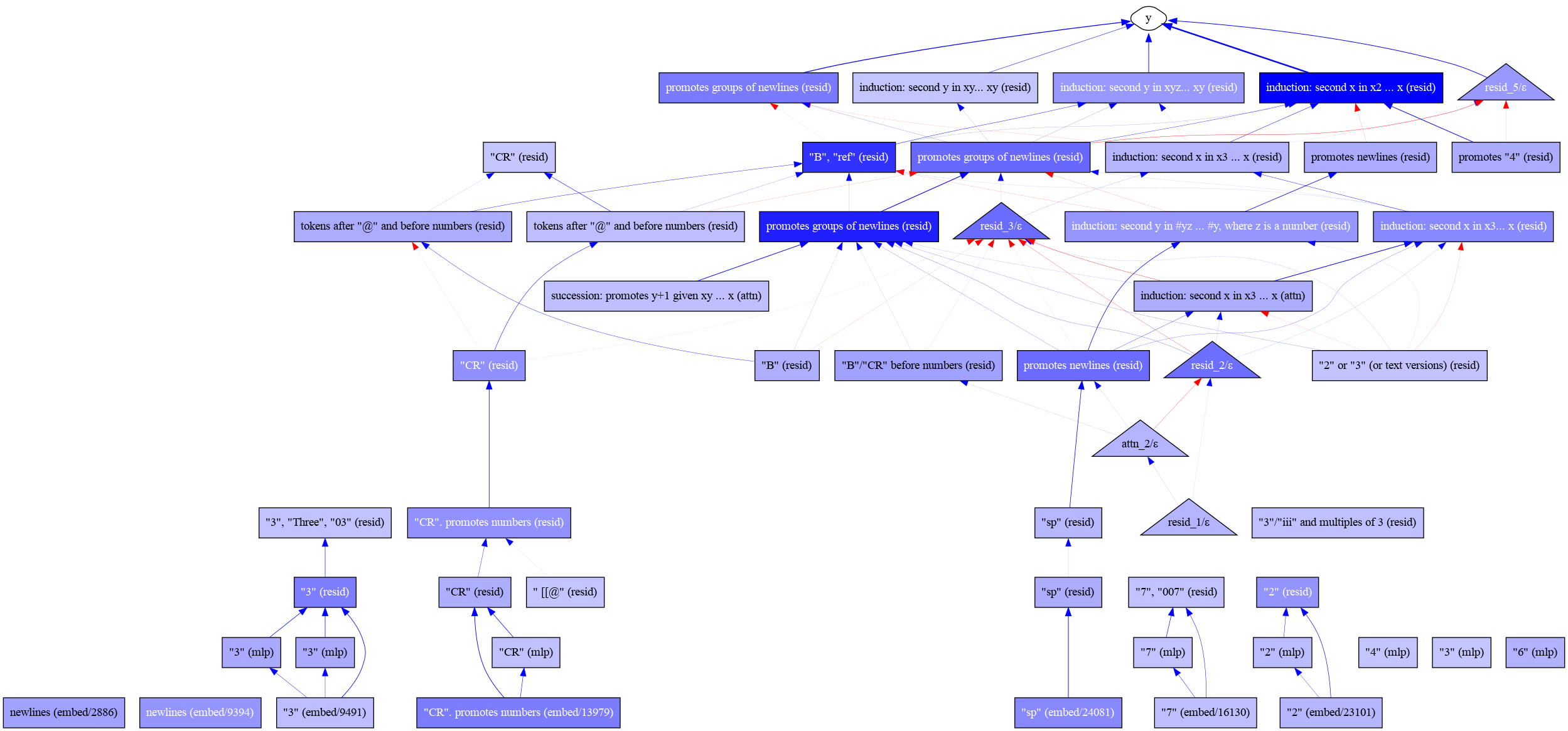<details> <summary>extracted/2403.19647v1/figures/circuits/cluster_382_contexts_dict10_node0.4_edge0.04_n10_aggsum_annotated.png Details</summary>  ### Visual Description ## Flowchart: Computational Rule Interactions ### Overview The flowchart depicts a hierarchical network of computational rules and their interactions, centered around a core node labeled "y". It illustrates dependencies between syntactic elements (e.g., "CR", "B"), numerical tokens, and embedded representations (e.g., "embed/2886"). Arrows indicate directional relationships, with red arrows highlighting exceptions or overrides. ### Components/Axes - **Core Node**: "y" (central hub) - **Primary Connections**: - "promotes groups of newlines (resid)" - "induction: second y in xy... xy (resid)" - "induction: second x in x2... xy (resid)" - **Secondary Nodes**: - "B / CR before numbers (resid)" - "promotes newlines (resid)" - "induction: second x in x3... x (resid)" - **Embedded Representations**: - "newlines (embed/2886)" - "newlines (embed/9394)" - "3" (embed/9491) - "2" (embed/23101) - "7" (embed/16130) - **Symbolic Nodes**: - "sp" (embed/24081) - "3" (mlp) - "2" (mlp) - "4" (mlp) - "6" (mlp) ### Detailed Analysis 1. **Core Node "y"**: - Connects to 5 primary nodes via blue arrows - Governs induction rules (e.g., "second y in xy... xy") - Links to "B / CR before numbers" and "promotes newlines" 2. **B / CR before numbers (resid)**: - Branches into "B (resid)" and "promotes newlines" - "B (resid)" connects to "B" and "promotes newlines" 3. **Numerical Tokens**: - "3" has 3 representations: residue, MLP, and embedding - "2" and "7" follow similar patterns with MLP/embedding variants - "sp" connects to both residue and embedding forms 4. **CR (Contextual Rules)**: - "CR" (resid) and "CR" (mlp) connect to "CR" (embed/13979) - "CR" promotes numbers via residue and MLP pathways 5. **Embedding Patterns**: - Numerical tokens have distinct embeddings (e.g., "3" embed/9491) - Newlines have two embeddings (2886, 9394) - Symbols like "sp" have dual representations ### Key Observations - **Hierarchical Structure**: "y" acts as the root node with cascading dependencies - **Redundancy**: Multiple pathways exist for numerical tokens (e.g., "3" has 3 representations) - **Symbolic Complexity**: "sp" and "CR" nodes show layered processing - **Embedding Diversity**: At least 5 distinct embeddings exist for numbers/symbols ### Interpretation This flowchart likely represents a computational grammar or parser rule set, where: 1. **y** serves as the primary syntactic element governing induction rules 2. **B** and **CR** nodes handle contextual processing before numerical tokens 3. **Embeddings** suggest machine learning integration for token representation 4. **MLP** (Multi-Layer Perceptron) connections indicate neural network processing 5. **Red arrows** may represent exception cases or rule overrides The system appears designed to process text through multiple representation layers (residue, MLP, embeddings) while maintaining syntactic relationships. The "promotes newlines" nodes suggest line-breaking rules, while induction rules handle variable substitution patterns (e.g., "second y in xy... xy"). </details> Figure 16: The full annotated feature circuit for incrementing number sequences. The model first detects the presence of specific number tokens, like “3”. Later, it learns more robust semantic representations of those numbers, like “iii” and “Three”. Then, the model uses a series of narrow and general succesion and induction features to increment the next number. 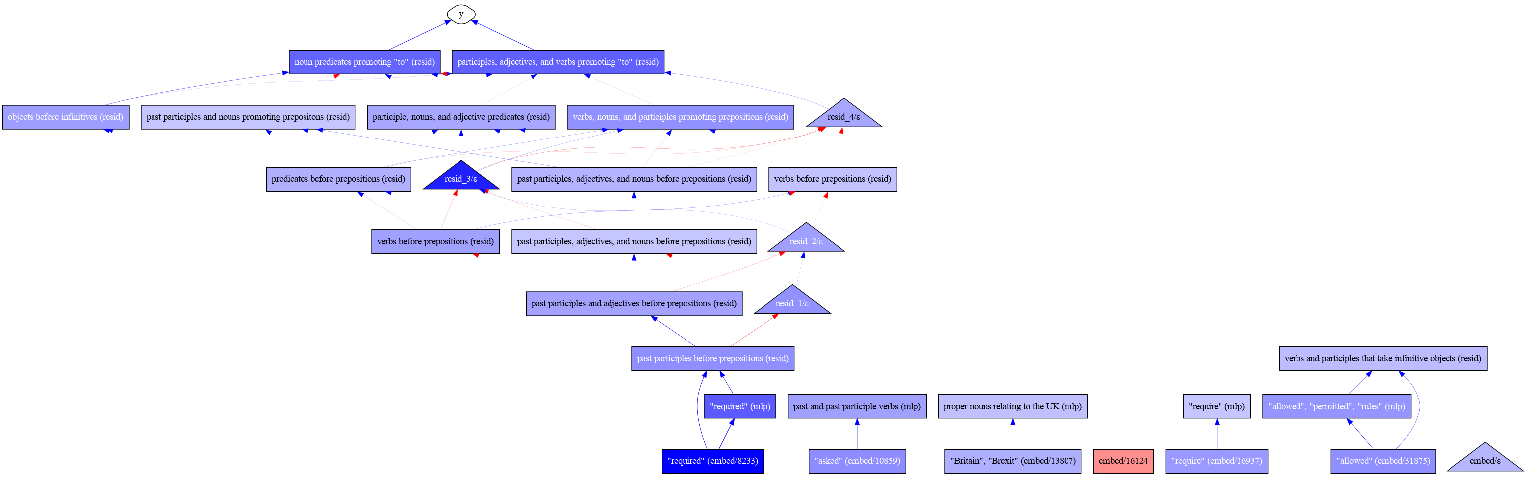<details> <summary>extracted/2403.19647v1/figures/circuits/cluster_475_contexts_dict10_node0.25_edge0.01_n6_aggsum_annotated.png Details</summary>  ### Visual Description ## Flowchart: Grammatical and Semantic Relationships with Embeddings ### Overview The image is a complex flowchart depicting hierarchical relationships between grammatical structures (e.g., nouns, verbs, participles) and their semantic embeddings. It includes nodes labeled with linguistic terms, prepositions, and embedding codes, connected by directional arrows. Triangles labeled with "resid_3/ε", "resid_4/ε", etc., appear to represent categorical or hierarchical groupings. ### Components/Axes - **Nodes**: - "noun predicates promoting 'to' (resid)" - "participles, adjectives, and verbs promoting 'to' (resid)" - "objects before infinitives (resid)" - "past participles and nouns promoting prepositions (resid)" - "participle, nouns, and adjective predicates (resid)" - "verbs, nouns, and participles promoting prepositions (resid)" - "predicates before prepositions (resid)" - "verbs before prepositions (resid)" - "past participles, adjectives, and nouns before prepositions (resid)" - "past participles and adjectives before prepositions (resid)" - "past participles before prepositions (resid)" - "required" (embed/8233) - "asked" (embed/10859) - "Britain", "Brexit" (embed/13807) - "require" (embed/16937) - "allowed", "permitted", "rules" (mlp) - "verbs and participles that take infinitive objects (resid)" - "allowed" (embed/31875) - "embed/ε" (triangle) - **Triangles**: - "resid_3/ε" - "resid_4/ε" - "resid_2/ε" - "resid_1/ε" - "embed/ε" - **Arrows**: - Blue arrows indicate hierarchical or causal relationships (e.g., "noun predicates promoting 'to' (resid)" → "objects before infinitives (resid)"). - Red arrows highlight specific dependencies (e.g., "resid_3/ε" → "resid_4/ε"). ### Detailed Analysis - **Grammatical Structures**: - Nodes like "noun predicates promoting 'to' (resid)" and "participles, adjectives, and verbs promoting 'to' (resid)" suggest a focus on verbs and their modifiers that govern infinitives. - "Objects before infinitives (resid)" and "past participles before prepositions (resid)" indicate positional relationships in sentence structure. - **Embeddings**: - Words like "required" (embed/8233), "asked" (embed/10859), and "Britain", "Brexit" (embed/13807) are linked to specific embedding codes, implying a computational model (e.g., word embeddings or machine learning parameters). - "require" (embed/16937) and "allowed" (embed/31875) suggest semantic or syntactic roles in the model. - **Hierarchical Groupings**: - Triangles labeled "resid_3/ε", "resid_4/ε", etc., may represent tiers of grammatical categories or residual components in a parsing model. - "embed/ε" (triangle) could denote a base or undefined embedding category. ### Key Observations - **Red Arrows**: Highlight critical dependencies, such as "resid_3/ε" → "resid_4/ε" and "resid_2/ε" → "resid_1/ε", suggesting a stepwise refinement or categorization process. - **Embedding Codes**: Numerical values (e.g., 8233, 10859) likely correspond to pre-trained embeddings or model parameters. - **Semantic Roles**: Terms like "allowed", "permitted", and "rules" (mlp) imply a focus on permission or constraint-based grammar. ### Interpretation The flowchart appears to model a **grammatical parsing or semantic analysis system**, where: 1. **Grammatical Relationships**: Nodes represent syntactic structures (e.g., prepositions, participles) and their roles in sentence formation. 2. **Embedding Integration**: Words and phrases are mapped to numerical embeddings, suggesting a machine learning or NLP framework. 3. **Hierarchical Categorization**: Triangles ("resid_3/ε", etc.) may denote layers of abstraction or residual components in a parsing algorithm. **Notable Patterns**: - The emphasis on "prepositions" and "infinitives" suggests a focus on complex syntactic structures. - The inclusion of "Britain" and "Brexit" (embed/13807) implies domain-specific or contextual embeddings. - The "required" (embed/8233) and "asked" (embed/10859) nodes might represent high-frequency or contextually significant terms. **Anomalies**: - The "embed/ε" triangle lacks a clear label, possibly indicating an undefined or placeholder category. - The "mlp" (multi-layer perceptron) label on "allowed", "permitted", and "rules" suggests a neural network component, but its exact role is unclear without additional context. This diagram likely serves as a visual representation of a computational model for analyzing or generating grammatical structures, with embeddings capturing semantic and syntactic relationships. </details> Figure 17: The full annotated feature circuit for predicting “to” as an infinitival object. The model first detects the presence of verbs that often take infinitival objects. Then, it uses one mechanism to detect present-tense verbs, participles, or predicate adjectives which take infinitival objects, and another mechanism to detect direct objects that can directly precede infinitival object complements. Finally, these two mechanisms both influence the output in layer 5 without fully intersecting. ## Appendix G Sample Features ### G.1 Sparse Features Here, we present examples of sparse features with high indirect effects on the Bias in Bios task. Some of these features clearly activate on terms related to medicine or academia, which are related to the target profession classification task. Others simply detect the presence of “he” or female names. 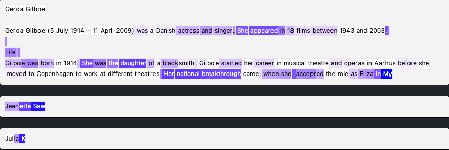<details> <summary>extracted/2403.19647v1/figures/example_features/sparse_attn_3_22029.png Details</summary>  ### Visual Description ## Screenshot: Wikipedia-like Textual Content ### Overview The image displays a structured textual excerpt resembling a Wikipedia page, divided into three sections. Each section contains a name in bold, followed by biographical details. The text is color-coded (white, purple, blue) for emphasis, with no visual charts or diagrams. ### Components/Axes - **Names**: - Gerda Gilboe (bold, white text) - Jeanette Saw (bold, purple text) - Julia K (bold, white text) - **Text Blocks**: - Gerda Gilboe’s entry includes birth/death dates, profession, filmography, and career history. - Jeanette Saw and Julia K have minimal text (only their names). - **Color Coding**: - White: Neutral text. - Purple: Highlighted phrases (e.g., "actress and singer," "national breakthrough"). - Blue: Key terms (e.g., "Eliza," "My"). ### Detailed Analysis #### Gerda Gilboe - **Text**: "Gerda Gilboe (5 July 1914 – 11 April 2009) was a Danish actress and singer. She appeared in 18 films between 1943 and 2003. Life Gilboe was born in 1914. She was the daughter of a blacksmith. Gilboe started her career in musical theatre and operas in Aarhus before she moved to Copenhagen to work at different theatres. Her national breakthrough came, when she accepted the role as Eliza in My." - **Key Details**: - Birth: 5 July 1914. - Death: 11 April 2009. - Profession: Actress, singer. - Filmography: 18 films (1943–2003). - Career: Began in Aarhus; moved to Copenhagen; breakthrough role as Eliza. #### Jeanette Saw and Julia K - **Text**: - Jeanette Saw: Only the name is visible (no additional details). - Julia K: Only the name is visible (no additional details). ### Key Observations 1. **Structural Hierarchy**: - Gerda Gilboe’s entry is the most detailed, suggesting she is the primary subject. - Jeanette Saw and Julia K lack descriptive text, possibly indicating incomplete data or placeholders. 2. **Color Usage**: - Purple and blue highlights emphasize critical career milestones (e.g., "national breakthrough," "Eliza"). 3. **Incomplete Information**: - The phrase "in My" under Gerda’s entry is truncated, likely a formatting error (e.g., missing title like "My Fair Lady"). ### Interpretation The text focuses on Gerda Gilboe’s career trajectory, highlighting her transition from Aarhus to Copenhagen and her defining role as Eliza. The truncated phrase "in My" suggests a missing reference to a film or production title, which could be critical for contextual accuracy. The brevity of Jeanette Saw and Julia K’s entries implies either incomplete data or a focus on Gerda as the central figure. The color-coding system appears to prioritize key achievements, though its application is inconsistent (e.g., "My" is blue but lacks context). ## Conclusion The image provides fragmented biographical data, with Gerda Gilboe’s entry being the most comprehensive. Further verification is needed to resolve formatting errors (e.g., "in My") and to expand details for Jeanette Saw and Julia K. </details> Figure 18: An example sparse feature from the Bias in Bios task (attn_3/22029). This feature detects female-related words in biographies of women. It also promotes words like “husband” and “née”. This feature probably contributes to preferences for the spurious correlate of gender; we therefore ablate it. <details> <summary>extracted/2403.19647v1/figures/example_features/sparse_resid_2_31098.png Details</summary>  ### Visual Description ## Screenshot: Textual Content ### Overview The image displays a screenshot of a document divided into two sections by a horizontal black line. The content focuses on two topics: 1. **Debbie Gregory** (DNP, RN), a healthcare design leader. 2. **Computer-assisted learning (CAL)** in nursing education. ### Components/Axes - **Section 1 (Top)**: - **Header**: "Debbie Gregory DNP, RN" in bold, with "DNP, RN" highlighted in light purple. - **Body**: A paragraph describing her role as a national leader in healthcare design, innovation, and transformation. Key terms like "nurse executive," "interior designer," and "Intentional Design" are bolded. - **Footer**: Details her academic credentials, including a Doctorate of Nursing Practice in Health Innovation and Leadership from the University of Minnesota and a bachelor’s in nursing. - **Section 2 (Bottom)**: - **Header**: "Computer assisted learning: the potential for teaching and assessing in nursing." - **Body**: A paragraph discussing CAL’s application in nursing education, referencing the Teaching and Learning Technology Programme (TLTP) and its influence on CAL. Terms like "nurse education" and "nursing" are bolded. ### Detailed Analysis - **Section 1 Text**: - Debbie Gregory is described as a leader in healthcare design, innovation, and transformation. - She is a nurse executive and interior designer who applies "Intentional Design" to align People, Place, and Process. - Her work involves transforming environments into functional ecosystems using complex systems science and strategic thinking. - Academic credentials: Doctorate of Nursing Practice (DNP) in Health Innovation and Leadership (University of Minnesota) and a bachelor’s in nursing. - **Section 2 Text**: - Focuses on CAL’s role in nursing education, emphasizing its importance and alignment with technological advancements. - Mentions the TLTP as a source of ideas for CAL’s application and benefits in nursing. ### Key Observations - The document uses bold formatting to emphasize key terms (e.g., "nurse," "nursing", "Intentional Design"). - The black line visually separates the two distinct topics. - The light purple highlight on "DNP, RN" draws attention to Debbie Gregory’s credentials. - Both sections emphasize the intersection of nursing and technology/design. ### Interpretation - **Debbie Gregory’s Profile**: The text positions her as a multidisciplinary expert bridging healthcare design, nursing, and systems science. Her focus on "Intentional Design" suggests a holistic approach to creating functional environments, likely impacting patient care and operational efficiency. - **CAL in Nursing**: The second section highlights the growing integration of technology in nursing education, aligning with broader trends in digital learning. The reference to TLTP indicates a foundation in established educational frameworks, suggesting CAL’s potential to enhance teaching methodologies and assessment practices in nursing. - **Structural Clarity**: The use of formatting (bold, highlights, section separation) ensures readability and emphasizes critical concepts, making the document accessible for technical or academic audiences. </details> Figure 19: An example sparse feature from the Bias in Bios task (resid_2/31098). This feature activates on words related to nursing, including “RN” and “nurse”. This probably relates to the target task of profession prediction. We therefore keep it. ### G.2 Neurons For contrast, we also present examples of dense features—that is, neurons from MLPs, layer-end residuals, and the out-projection of the attention—with high indirect effects on the Bias in Bios task. We cannot directly interpret the activation patterns of these neurons, and so it is difficult to run the Shift with neurons baseline. We therefore instead compare to the neuron skyline, where we allow the skyline an unfair advantage by simply ablating neurons which have positive effects on gender-based probabilities given the balanced set. 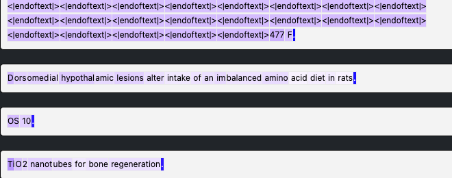<details> <summary>extracted/2403.19647v1/figures/example_features/dense_resid_1_111.png Details</summary>  ### Visual Description ## Screenshot: Text Editor with Highlighted Content ### Overview The image shows a text editor interface with multiple lines of text, some highlighted in purple. The content includes technical/scientific phrases, repeated placeholder tags (`</code>`), and formatting elements like horizontal black lines. ### Components/Axes - **Text Blocks**: - Repeated `</code>` tags (highlighted in purple) appear in three lines at the top. - A horizontal black line separates sections. - Scientific phrases: 1. "Dorsomedial hypothalamic lesions alter intake of an imbalanced amino acid diet in rats." (highlighted in purple) 2. "OS 10." (highlighted in purple) 3. "TiO2 nanotubes for bone regeneration." (highlighted in purple) - **Highlighting**: Purple highlights emphasize specific text segments, likely indicating importance or annotations. ### Detailed Analysis - **Top Section**: - Three lines of `</code>` tags (e.g., `</code>`) are repeated, suggesting placeholders or markers for text segmentation. - **Middle Section**: - The phrase "Dorsomedial hypothalamic lesions alter intake of an imbalanced amino acid diet in rats." is highlighted, indicating a focus on neuroscience or behavioral studies. - **Lower Sections**: - "OS 10." (highlighted) may reference an operating system version or a dataset identifier. - "TiO2 nanotubes for bone regeneration." (highlighted) points to materials science or biomedical engineering research. ### Key Observations - The repetition of `</code>` tags suggests automated text processing or model training data. - Highlighted text spans diverse fields (neuroscience, materials science, OS versions), implying a multidisciplinary document. - No numerical data or charts are present; the focus is on textual annotations. ### Interpretation The highlighted text likely represents key research topics or annotations within a larger dataset or document. The `</code>` tags may serve as delimiters for machine learning models to parse or generate text. The juxtaposition of scientific phrases suggests the document could be a research summary, dataset metadata, or a training corpus for NLP tasks. The lack of numerical trends or diagrams emphasizes textual categorization over quantitative analysis. </details> Figure 20: An example neuron from the Bias in Bios task. This appears to activate on beginnings and ends of sentences, but also more strongly on any token in a sentence that contains capital letters or numbers. We cannot deduce whether this would contribute more to gender or profession names. <details> <summary>extracted/2403.19647v1/figures/example_features/dense_resid_2_369.png Details</summary>  ### Visual Description ## Textual Content: Scientific and News Articles ### Overview The image contains two distinct blocks of text: 1. A scientific paragraph discussing inorganic phosphate (Pi) uptake mechanisms in plant cells. 2. A news snippet about disruptions to Delhi metro services. ### Content Details #### Scientific Text (Top Block) - **Key Terms**: - Inorganic phosphate (Pi) uptake - Vacuolar membrane - Catharanthus roseus suspension-cultured cells - H⁺ pumping - Pi status (low/high) - **Process Description**: - Under low Pi status, Pi uptake into vacuoles is strongly activated compared to high Pi status. - Pi uptake across the vacuolar membrane correlates with H⁺ pumping. - The study examines the dependency of H⁺ pumping on plant Pi status. #### News Text (Bottom Block) - **Event**: - Delhi metro services on the Blue Line were briefly disrupted. - Cause: A girl jumped in front of an approaching train. ### Key Observations - The scientific text focuses on cellular mechanisms of nutrient regulation in plants. - The news text describes a singular, localized incident affecting public transportation. ### Interpretation 1. **Scientific Context**: - The study highlights how plants regulate Pi uptake under nutrient-deficient (low Pi) vs. sufficient (high Pi) conditions. - The correlation between Pi uptake and H⁺ pumping suggests an active transport mechanism, likely involving proton gradients. 2. **News Context**: - The disruption underscores risks associated with human behavior near railway systems. - No quantitative data (e.g., duration of disruption, casualties) is provided in the text. 3. **Cross-Text Analysis**: - Both texts involve "disruption" but in vastly different contexts: biological regulation vs. human-caused transportation delays. ### Notes on Data Extraction - No charts, diagrams, or numerical data are present. - All text is in English; no foreign languages detected. - No spatial or visual elements (e.g., axes, legends) to analyze. </details> Figure 21: An example neuron from the Bias in Bios task. This activates positively on tokens starting with capital letters, but negatively on many other tokens (whose unifying theme we cannot deduce). ## Appendix H Discovering LM Behaviors with Clustering In this section, we describe our unsupervised method for discovering language model behaviors. More specifically, following Michaud et al. (2023), we cluster contexts from The Pile according to the Pythia-70M’s internal state during inference. In this section, we describe our clustering pipeline and methods. ### H.1 Filtering Tokens We must first locate (context, answer) pairs for which an LM correctly predicts the answer token from the context. We select The Pile (Gao et al. (2020)) as a general text corpus and filter to pairs on which Pythia-70M confidently and correctly predicts the answer token, with cross-entropy lower than 0.1 or 0.3 nats, depending on the experiment. The model consistently achieves low loss on tokens which involve “induction” (Olsson et al., 2022) —i.e., tokens which are part of a subsequence which occurred earlier in the context. We exclude induction samples by filtering out samples in which the bigram (final context token, answer token) occured earlier in the context. ### H.2 Caching Model-internal Information We find behaviors by clustering samples according to information about the LM’s internals when run on that sample. We find clusters of samples where the model employs similar mechanisms for next-token prediction. We experiment with various inputs to the clustering algorithm: - Dense Activations: We take activations (residual stream vectors, attention block outputs, or MLP post-activations) from a given context and concatenate them. To obtain a vector whose length is independent of the context length, we can either use the activations at the last $N$ context positions before the answer token, or aggregate (sum) across the sequence dimension. We experiment with both variants. - Sparse Activations: Rather than dense model activations, we can use the activations of SAE features. We concatenate and aggregate these in the same manner as for dense activations. - Dense Component Indirect Effects: We approximate the indirect effect of all features on the correct prediction using 2 without a contrastive pair—namely, by setting ${a}_patch=0$ . The negative log-probability of the answer token $m=-\log p(answer)$ serves as our metric for the correct prediction of the next token. The computatiom of linear effects requires saving both (1) activations and (2) gradients w.r.t $m$ at the final $N$ positions for each context in the dataset. We optionally aggregate by summing over all positions. - Sparse Indirect Effects: Similarly, we can compute the linear effects of sparse activations on the correct prediction. - Gradient w.r.t. model parameters: As in Michaud et al. (2023), we also experiment with using gradients of the loss w.r.t. model parameters, but with some modifications. We describe this method in more detail in § H.3 below. ### H.3 Hyperparameters and Implementation Details We apply either spectral clustering or $k$ -means clustering. For spectral clustering, given either activations or effects $x_i$ for sample $i$ , we compute a matrix of pairwise cosine similarities $C_ij=x_i· x_j/(||x_i||||x_j||)$ between all pairs of samples. Before performing spectral clustering, we normalize all elements of $C$ to be in $[0,1]$ by converting the cosine similarities to angular similarities: $\hat{C}_ij=1-\arccos(C_ij)/π$ . We use the scikit-learn (Pedregosa et al., 2011) spectral clustering implementation with $k$ -means. For all inputs except gradients w.r.t. model parameters, we used spectral clustering across 8192 samples. We chose $k$ (the number of total clusters) to maximize the number of clusters implicated in more than one input context. We also experimented with using gradients w.r.t. model parameters as inputs, as in Michaud et al. (2023). Here, we scale up our approach to 100,000 samples. It is intractible to perform spectral clustering given 100,000 samples, so we instead use $k$ -means clustering. Rather than clustering the gradients themselves (which are high-dimensional), we cluster sparse random projections of the gradients down to 30,000 dimensions. When projecting, we use a matrix with entries $\{-1,0,1\}$ . When sampling the entries of this matrix, sample a nonzero value with probability $32/30000$ , and if nonzero, sample $-1$ or $1$ with equal probability. For a sparse projection matrix with dimensions ${ℝ}^n× 30000$ , there will on average be $32· n$ nonzero entries, where $n$ is the number of parameters in the model. We only consider gradients w.r.t. non-embedding and non-layernorm parameters.