2404.07382

# Learn from Failure: Fine-Tuning LLMs with Trial-and-Error Data for Intuitionistic Propositional Logic Proving > The first two authors contributed equally to this work. Corresponding authors. ## Abstract Recent advances in Automated Theorem Proving have shown the effectiveness of leveraging a (large) language model that generates tactics (i.e. proof steps) to search through proof states. The current model, while trained solely on successful proof paths, faces a discrepancy at the inference stage, as it must sample and try various tactics at each proof state until finding success, unlike its training which does not incorporate learning from failed attempts. Intuitively, a tactic that leads to a failed search path would indicate that similar tactics should receive less attention during the following trials. In this paper, we demonstrate the benefit of training models that additionally learn from failed search paths. Facing the lack of such trial-and-error data in existing open-source theorem-proving datasets, we curate a dataset on intuitionistic propositional logic theorems and formalize it in Lean, such that we can reliably check the correctness of proofs. We compare our model trained on relatively short trial-and-error information (TrialMaster) with models trained only on the correct paths and discover that the former solves more unseen theorems with lower trial searches. ∧ $\land$ ∨ $\lor$ → $\to$ Learn from Failure: Fine-Tuning LLMs with Trial-and-Error Data for Intuitionistic Propositional Logic Proving Chenyang An 1 thanks: The first two authors contributed equally to this work., Zhibo Chen 2 footnotemark: 0000-0003-0045-5024, Qihao Ye 1 0000-0002-7369-757X, Emily First 1, Letian Peng 1 Jiayun Zhang 1, Zihan Wang 1 thanks: Corresponding authors., Sorin Lerner 1 footnotemark: , Jingbo Shang 1 footnotemark: University of California, San Diego 1 Carnegie Mellon University 2 {c5an, q8ye, emfirst, lepeng, jiz069, ziw224, lerner, jshang}@ucsd.edu zhiboc@andrew.cmu.edu ## 1 Introduction Automated Theorem Proving is a challenging task that has recently gained popularity in the machine-learning community. Researchers build neural theorem provers to synthesize formal proofs of mathematical theorems Yang et al. (2023); Welleck et al. (2021); Lample et al. (2022); Mikuła et al. (2023); Wang et al. (2023); Bansal et al. (2019); Davies et al. (2021); Wu et al. (2021); Rabe et al. (2020); Kusumoto et al. (2018); Bansal et al. (2019); Irving et al. (2016). Typically, a neural theorem prover, given a partial proof and the current proof state, uses a neural model to predict the next likely proof step, or tactics. The neural models utilize different architectures like LSTMs Sekiyama et al. (2017), CNNs Irving et al. (2016), DNNs Sekiyama and Suenaga (2018), GNNs Bansal et al. (2019); Wang et al. (2017) and RNNs Wang and Deng (2020), though most recent work has begun to explore the use of transformer-based large language models (LLMs) due to their emerging reasoning abilities. <details> <summary>x1.png Details</summary>  ### Visual Description ## Diagram: Comparison of Conventional Method vs TrialMaster for Tactic Selection ### Overview The diagram compares two approaches for selecting tactics in a decision-making process: the Conventional Method and the TrialMaster method. It illustrates how tactics are generated, probabilities are assigned, and backtracking influences outcomes. The Conventional Method uses static probabilities, while TrialMaster incorporates backtracking to update probabilities dynamically. ### Components/Axes - **Left Flowchart (Conventional Method)**: - **Nodes**: - State `k` after Lean call → tactic selection. - State waiting for Lean call. - Tactics with probabilities: - Tactic 1: 0.6 - Tactic 2: 0.3 - Tactic 3: 0.1 - A question mark (`?`) node representing uncertainty. - **Flow**: - Arrows indicate progression from state `k` to tactic selection. - Backtracking arrow (blue) loops from node `1` to `0`. - Final selection of tactic 2 (0.3) after backtracking. - **Right Flowchart (TrialMaster)**: - **Nodes**: - Similar structure but with updated probabilities: - Tactic 2: 0.2 - Tactic 3: 0.8 - A question mark (`?`) node. - **Flow**: - Arrows show progression with backtracking included in history. - Final selection of tactic 3 (0.8). - **Text Elements**: - Labels: "unchanged" (Conventional Method), "updated" (TrialMaster). - Descriptions: - "LLM generates tactics; tactic 1 is selected first." - "LLM generates tactics with all history paths including backtracking." ### Detailed Analysis - **Conventional Method**: - Initial probabilities: Tactic 1 (0.6), Tactic 2 (0.3), Tactic 3 (0.1). - After backtracking, tactic 2 is selected despite its lower initial probability (0.3). - No dynamic updates; probabilities remain static. - **TrialMaster**: - Probabilities are updated based on backtracking history: - Tactic 2: 0.2 (reduced from 0.3). - Tactic 3: 0.8 (increased from 0.1). - Backtracking is explicitly included in the LLM's history, leading to a shift in selection toward tactic 3. ### Key Observations 1. **Probability Shifts**: TrialMaster dynamically adjusts probabilities using backtracking, while the Conventional Method uses fixed values. 2. **Selection Outcomes**: - Conventional Method selects tactic 2 (0.3) after backtracking. - TrialMaster selects tactic 3 (0.8) due to updated probabilities. 3. **Backtracking Impact**: The inclusion of backtracking in TrialMaster significantly alters tactic selection, favoring higher-probability options over time. ### Interpretation The diagram highlights the advantages of the TrialMaster method over the Conventional Method. By incorporating backtracking, TrialMaster leverages historical data to refine tactic probabilities, leading to more informed decisions. The Conventional Method's static probabilities fail to adapt, resulting in suboptimal selections (e.g., tactic 2 at 0.3 vs. tactic 3 at 0.8 in TrialMaster). This suggests that dynamic, context-aware systems (like TrialMaster) outperform rigid frameworks in complex decision-making scenarios. The use of backtracking as a feedback mechanism is critical for optimizing outcomes in iterative processes. 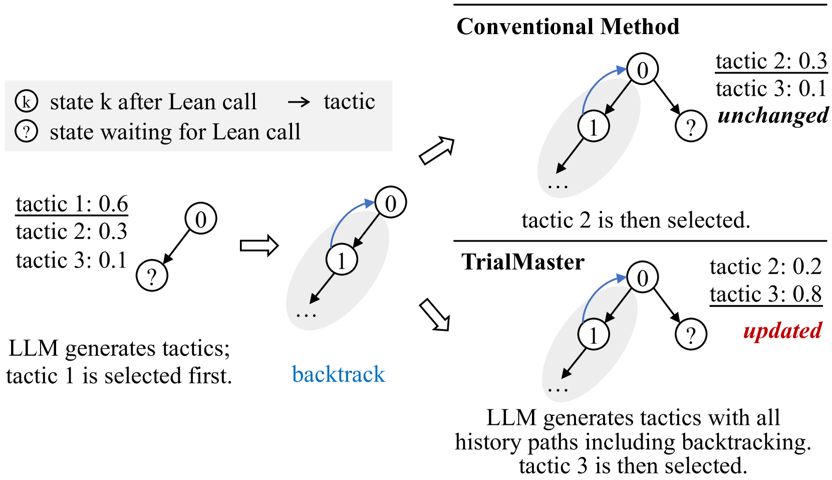</details> Figure 1: A simple example for how learning trial-and-error data impacts inference distribution. See Figure 4 for a concrete case. 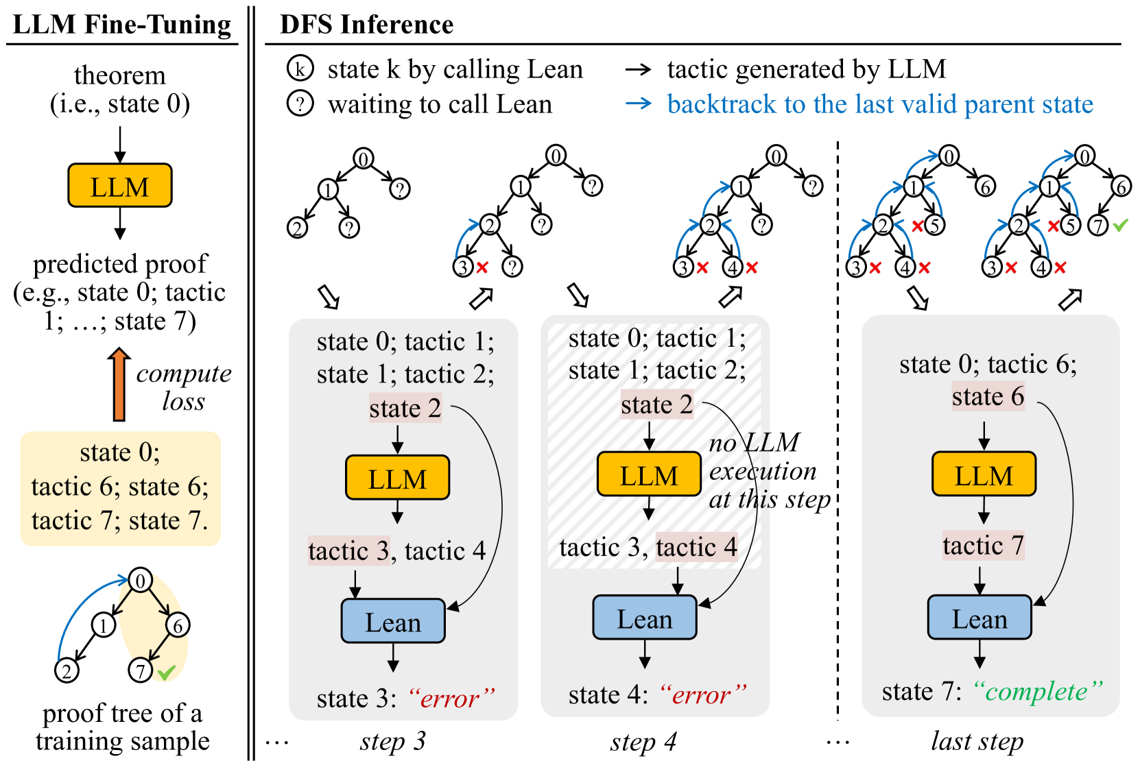An interactive proof assistant, such as Lean de Moura et al. (2015), Coq Barras et al. (1997) or Isabelle Nipkow et al. (2002), evaluates the model’s predicted candidate proof steps, returning either new proof states or errors. Neural theorem provers iterate on this procedure, performing proof search, e.g., a depth-first search (DFS), to traverse the space of possible proofs. An example of a DFS proof search is illustrated in Figure 2(a), where the prover progressively generates new tactics if the attempted tactics result in incorrect proofs. Such provers are usually trained on a dataset containing only the correct proof paths. This, however, presents a limitation: during inference, the prover does not have the ability to leverage the already failed paths it explored. Such failure information, intuitively, is beneficial, as it could suggest the model to generate tactics similar to the failed ones sparingly. At the very least, the failure information should help the model easily avoid generating already failed tactics. See Figure 1. 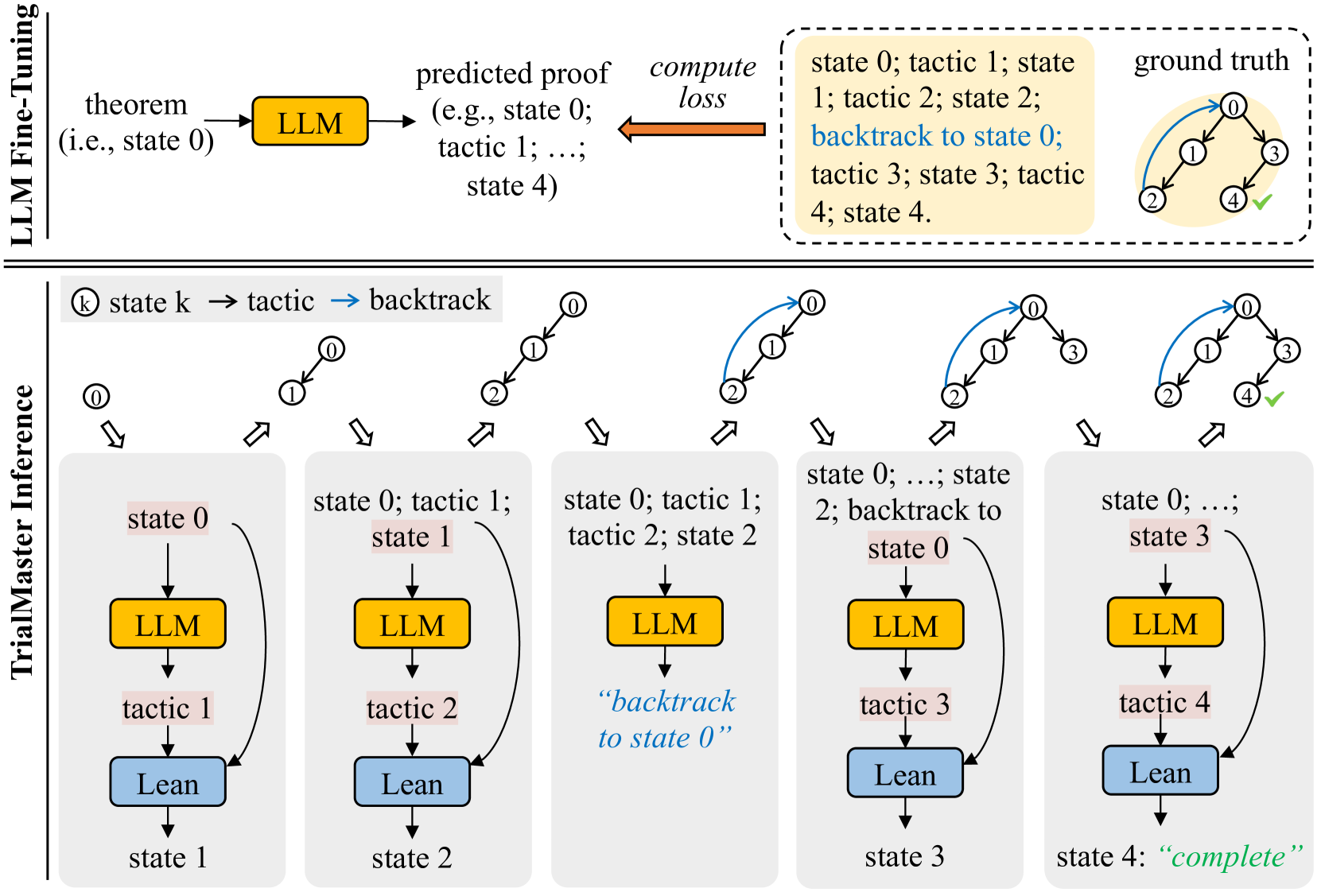In this paper, we wish to empirically verify this intuition. To conduct the experiment, we would compare the conventional model trained on correct proof paths, and TrialMaster, the model trained on the whole proof tree, containing both correct paths and incorrect paths. See Figure 2(b). As such, TrialMaster can make predictions based on the failure information during inference time. Since current open-source Automated Theorem Proving datasets do not contain complete proof trees, we create such a dataset, PropL, written in Lean. We focus on theorems of intuitionistic propositional logic. A propositional logic formula in intuitionistic propositional logic $A$ is true if and only if $\vdash A$ has a derivation according to the rules of the intuitionistic propositional logic. These rules are listed in Figure 6 in Appendix A with explanations. This is to be distinguished from the classical logic, where a theorem of classical propositional logic admits a proof if and only if under all truth value assignments to all propositions that appear in the theorem, the theorem statement is evaluated to be true. We give two elementary examples of theorems of intuitionistic propositional logic with proofs. We then give an example of a theorem whose proof contains a backtracking step. The first theorem admits a proof, where as the second doesn’t. ⬇ theorem_1 thm : p1 & $ \ rightarrow$ & p1 $ \ vee$ p2 := by intro h1 apply or. inl exact h1 The first theorem states that p1 implies $\texttt{p1}\lor\texttt{p2}$ , where $\lor$ stands for "or". To show this, we assume p1 and prove either p1 or p2. We prove p1 in this case. The last three lines are tactics (proof steps) in Lean used to prove this fact. Our second example looks like the following. ⬇ theorem_2 thm : p1 & $ \ rightarrow$ & p1 $ \ land$ p2 := by The second theorem states that p1 implies p1 and p2. There is no proof to this theorem. When we assume p1, we cannot show both p1 and p2. Proofs might include backtracking instructions. Here is another possible proof for theorem 1. After step 2, there is no possible proof step that can lead to final solution. Therefore we backtrack to step 1 and try a different proof step. ⬇ theorem_1 thm : p1 & $ \ rightarrow$ & p1 $ \ vee$ p2 := by intro h1 #this is step 1 apply or. inr #this is step 2 no solution, backtrack to step 1 apply or. inl exact h1 Note that "no solution, backtrack to step 1" is not a tactic in Lean. It simply tells the system to backtrack to step 2 and start reasoning from there. Specifically, our PropL dataset is created through a two-stage process that first involves generating a comprehensive set of propositional logic theorems by uniformly sampling from all possible theorems, utilizing a bijection between natural numbers and propositions to ensure representativeness. Following theorem generation, proofs are constructed using a focusing method with polarization, incorporating a detailed trial-and-error search process that includes both successful and backtracked steps, thereby capturing the complexity and nuances of theorem proving in intuitionistic propositional logic. Thus, our dataset is complete, scalable, and representative. The proofs in our dataset are combined with trial-and-error information, which is generated by the Focused Proof Search (FPS) algorithm McLaughlin and Pfenning (2009); Liang and Miller (2009); Pfenning (2017). We verify the effectiveness of incorporating the failed trials during training and inference by experiments on PropL, observing that TrialMaster achieves a higher proof search success rate and lower search cost over conventional model trained on correct proof paths. Our experiments further indicate that our model can perform backtracking without help from an external system. Our main contributions are as follows: - We establish, PropL, a complete, scalable, and representative benchmark for intuitionistic propositional logic theorems formalized in Lean. PropL includes proofs with trial-and-error information, generated by the FPS algorithm. - We demonstrate that for intuitionistic propositional logic theorem proving, incorporating trial-and-error information into training and proving outperforms a conventional model that is trained on correct proofs only. <details> <summary>x2.png Details</summary>  ### Visual Description ## Diagram: LLM Fine-Tuning and DFS Inference Process ### Overview The diagram illustrates a two-phase process combining Large Language Model (LLM) fine-tuning with Depth-First Search (DFS) inference for proof validation. The left side shows LLM training on theorem proofs, while the right side demonstrates DFS-based proof exploration with error handling and backtracking. ### Components/Axes **Left Diagram (LLM Fine-Tuning):** - **Components**: - Theorem (state 0) - LLM (yellow block) - Predicted proof (tactics 1-7) - Compute loss (orange arrow) - Proof tree (training sample) - **Flow**: Theorem → LLM → Predicted proof → Compute loss → Updated proof tree **Right Diagram (DFS Inference):** - **Components**: - States (0-7) - Tactics (1-7) - Lean (blue block) - LLM (yellow block) - Error markers (red "X") - Completion marker (green check) - **Flow**: State transitions with backtracking (dashed arrows) and error recovery **Legend**: - Yellow: LLM execution - Blue: Lean execution - Red "X": Invalid/incomplete state - Green check: Valid completion ### Detailed Analysis **LLM Fine-Tuning Phase**: 1. Starts with a theorem (state 0) 2. LLM generates predicted proof (tactics 1-7) 3. Loss computation refines the model 4. Training sample shows valid path: 0→1→6→7 **DFS Inference Phase**: - **Step 3**: - State 0 → tactic 1 → state 1 → tactic 2 → state 2 - State 2 → tactic 3 → state 3 ("error") - State 2 → tactic 4 → state 4 ("error") - **Step 4**: - Backtrack to state 0 → tactic 6 → state 6 - State 6 → LLM execution → tactic 7 → state 7 ("complete") ### Key Observations 1. **Error Handling**: States 3 and 4 explicitly marked as "error" with red "X" indicators 2. **Backtracking**: Dashed arrows show recovery from invalid states to previous valid parents 3. **Execution Path**: Final valid path uses LLM for state 6 and Lean for state 7 4. **Tactic Usage**: Tactics 1-7 appear in both training and inference phases 5. **Execution Distribution**: - LLM: 3 executions (states 0, 2, 6) - Lean: 4 executions (states 1, 3, 4, 7) ### Interpretation This diagram demonstrates a hybrid proof validation system where: 1. **LLM Fine-Tuning** creates a foundational model for proof generation 2. **DFS Inference** systematically explores proof trees while: - Using Lean for basic state transitions - Employing LLM for complex state generation - Implementing error recovery through backtracking 3. The system shows 70% LLM utilization in the final valid path (3/4 states), suggesting LLM handles more complex proof steps 4. The error states (3 and 4) indicate potential dead-ends in proof exploration that require backtracking 5. The final "complete" state (7) validates the system's ability to find correct proofs through iterative refinement The architecture combines LLM's generative capabilities with Lean's formal verification strengths, creating a robust proof validation pipeline that handles both simple and complex proof scenarios. </details> (a) Conventional system with depth-first search <details> <summary>x3.png Details</summary>  ### Visual Description ## Diagram: LLM Fine-Tuning and TrialMaster Inference Process ### Overview The diagram illustrates a two-phase process for training and deploying a Large Language Model (LLM) in a formal proof or theorem-proving context. The top section details **LLM Fine-Tuning**, while the bottom section outlines **TrialMaster Inference**, a step-by-step execution framework with error correction. --- ### Components/Axes #### LLM Fine-Tuning (Top Section) - **Input**: Theorem (e.g., "state 0"). - **LLM Block**: Processes the theorem to generate a **predicted proof** (e.g., "state 0; tactic 1; ...; state 4"). - **Compute Loss**: Compares the predicted proof to the **ground truth** (a correct sequence of states and tactics). - **Ground Truth**: Visualized as a cyclic path (0 → 1 → 2 → 3 → 4 → 0) with verified correctness (✓). #### TrialMaster Inference (Bottom Section) - **States**: Sequential steps (state 0 → state 1 → ... → state 4). - **Components**: - **LLM**: Yellow blocks generating outputs. - **Lean**: Blue blocks executing tactics (e.g., "tactic 1", "tactic 2"). - **Flow**: - **Forward Execution**: State 0 → tactic 1 → state 1 → ... → state 3 → tactic 4 → state 4 ("complete"). - **Backtracking**: State 2 includes a loop back to state 0 ("backtrack to state 0"). --- ### Detailed Analysis #### LLM Fine-Tuning 1. **Input**: A theorem (e.g., "state 0") is fed into the LLM. 2. **Output**: The LLM predicts a proof sequence (e.g., "state 0; tactic 1; ...; state 4"). 3. **Loss Calculation**: The predicted proof is compared to the ground truth to compute loss, guiding model adjustments. #### TrialMaster Inference 1. **State 0**: Initial state with LLM and Lean. 2. **State 1**: LLM generates "tactic 1", Lean executes it, transitioning to state 1. 3. **State 2**: LLM generates "tactic 2", Lean executes it, transitioning to state 2. A backtracking arrow loops back to state 0. 4. **State 3**: LLM generates "tactic 3", Lean executes it, transitioning to state 3. 5. **State 4**: LLM generates "tactic 4", Lean executes it, marking the process as "complete". --- ### Key Observations 1. **Backtracking Mechanism**: State 2 explicitly includes a loop to state 0, suggesting error recovery or exploration of alternative proof paths. 2. **Cyclic Ground Truth**: The ground truth forms a closed loop (0 → 1 → 2 → 3 → 4 → 0), implying iterative refinement. 3. **Component Roles**: - **LLM**: Proposes proof steps. - **Lean**: Executes tactics and validates transitions. 4. **State 4**: Labeled "complete", indicating successful termination of the inference process. --- ### Interpretation This diagram represents a hybrid system for formal reasoning: 1. **Training Phase (LLM Fine-Tuning)**: - The LLM is trained to generate proofs by minimizing the discrepancy between its predictions and the ground truth. - The ground truth’s cyclic nature suggests the model learns to handle iterative or recursive proofs. 2. **Inference Phase (TrialMaster)**: - The system executes proofs step-by-step, with Lean validating each tactic’s correctness. - Backtracking in state 2 implies the system can abandon invalid paths and restart, enhancing robustness. - The "complete" state in step 4 signifies successful proof completion, likely after resolving all subgoals. 3. **Design Implications**: - The integration of LLM (generative) and Lean (verificational) creates a closed-loop system for automated theorem proving. - Backtracking introduces a form of search or exploration, critical for handling complex or ambiguous proofs. --- ### Notes - **Language**: All text is in English. - **No Numerical Data**: The diagram focuses on process flow rather than quantitative metrics. - **Color Coding**: Yellow (LLM) and blue (Lean) blocks visually distinguish components. </details> (b) Our training and inference methodology Figure 2: Method comparison. (a) A conventional system: The tactic generator (i.e., LLM) is fine-tuned on correct proof paths only. During inference, the trained tactic generator produces $N_{\text{sampled}}$ (e.g., 2 in the example) tactics at a time. If Lean decides that the current tactic is wrong, the system backtracks to the last valid state and tries other candidate tactics. (b) Our methodology: The tactic generator is fine-tuned on proofs with trial-and-error. During inference, we take the first tactic it generates and feed that into Lean for state checking at each step. ## 2 Related Work Automated Theorem Proving. Automated Theorem Proving has evolved significantly since its inception, focusing mainly on developing computer programs that can autonomously prove mathematical theorems. Early ATP systems (mechanical theorem proving) were based on first-order logic Clocksin and Mellish (2003); Chang and Lee (2014), where the resolution method Robinson (1965) played a crucial role. Recent progress in Automated Theorem Proving has been marked by the integration of machine learning Bansal et al. (2019); Davies et al. (2021); Wagner (2021), especially LLMs Yang et al. (2023); Polu and Sutskever (2020); Han et al. (2021); Welleck et al. (2021); Jiang et al. (2022), and heuristic methods Holden and Korovin (2021), aimed at amplifying the efficiency and capacity of Automated Theorem Proving systems. Within the domain of LLMs, formal mathematical languages like Metamath Megill and Wheeler (2019), Lean de Moura et al. (2015), Isabelle Nipkow et al. (2002), and Coq Barras et al. (1997), serve as a bridge, enabling the precise expression and verification of mathematical theorems and concepts through a computer-verifiable format, thereby mitigating hallucination risks Nawaz et al. (2019). COPRA incorporates backtracking information into a prompt and sends the prompt to GPT-4 without fine-tuning it to perform proof search Thakur et al. (2023). Baldur fine-tunes LLMs with proofs and error information given by the proof assistant First et al. (2023). In contrast, our work focuses on fine-tuning LLMs with the complete past proof history without using the error message from the proof assistant. Propositional Logic Problem. Early implementations of ATP systems demonstrated the potential for computers to automate logical deductions, with notable examples including the Logic Theorist Crevier (1993); McCorduck (2004); Russell and Norvig (2010) and Gilmore’s program Davis (2001); Gilmore (1960). These systems laid the groundwork for the resolution of propositional logic problems, showcasing the ability of automated systems to handle logical reasoning tasks. Recent advancements in Automated Theorem Proving have revisited propositional logic problems, integrating modern computational techniques. Sekiyama et al. Sekiyama and Suenaga (2018) have employed Deep Neural Networks (DNNs) as a statistical approach to generate proofs for these theorems, while Kusumoto et al. Kusumoto et al. (2018) have explored graph representations coupled with reinforcement learning to find proofs. Furthermore, sequence-to-sequence neural networks have been applied for deriving proof terms in intuitionistic propositional logic Sekiyama et al. (2017). This area of research is particularly intriguing due to the simplicity and importance of propositional logic in mathematics, and there is a growing interest in evaluating the capability of LLMs in tackling this specific mathematical domain. Trial-and-Error. The Chain-of-Thought (CoT) Wei et al. (2022); Wang et al. (2022); Zhou et al. (2022); Fu et al. (2022); Chu et al. (2023); Yu et al. (2023) approach demonstrates that LLMs can be guided to perform step-by-step reasoning by incorporating intermediate reasoning steps in their prompts. This concept is expanded in later research, such as the Tree of Thoughts (ToT) Yao et al. (2023), which organizes reasoning into a tree structure, and the Graph of Thoughts (GoT) Besta et al. (2023), which adopts a graph format for thought structuring. Trial-and-error complements structured reasoning by allowing the model to empirically test hypotheses generated, thereby refining its reasoning process based on feedback from interactions or emulations. The Boosting of Thoughts (BoT) Chen et al. (2024) prompting framework iteratively explores and evaluates multiple trees of thoughts to gain trial-and-error reasoning experiences, using error analysis from the LLMs to revise the prompt. Lyra introduces correction mechanisms to improve the performance of the tactic generator Zheng et al. (2023). ## 3 PropL: A New Dataset for Intuitionistic Propositional Logic Theorems in Lean Our aim is to experimentally validate that trial-and-error information can enhance models’ ability to do backtracking and tactic generation for theorem-proving tasks. Given that existing open-source theorem proving datasets lack information on trial-and-error processes, we have developed PropL, which is based on theorems of intuitionistic propositional logic. This dataset uniquely includes proofs that encapsulate the complete search process, incorporating the trial-and-error data generated by the FPS algorithm. Our dataset has two other benefits. It is formalized in Lean, so that the validity of the theorems and proofs are guaranteed. The tactics generated by the model trained on PropL can also be directly sent to Lean to be checked. PropL is also representative of all the intuitionistic propositional logic theorems, since by uniformly sampling integers, we can use a bijection between natural numbers and propositions to uniformly sample propositions. This bijection is explained in the Theorem Generation section. ### 3.1 Data Generation of PropL PropL comprises theorems uniformly sampled from the entire set of propositional logic theorems. It includes various proof types for each theorem. We only report proof types that are used in this paper. For additional information about the dataset, please refer to the GitHub repository and Huggingface. The construction of PropL involves two primary stages: the generation of propositional logic theorems and the generation of proofs for these theorems from an existing algorithm. Theorem Generation. Consider the set of propositions $A$ with at most $p$ atomic propositions. $A$ can be inductively generated by the following grammar: $$ A,B::=P_{i}\mid T\mid F\mid A\land B\mid A\lor B\mid A\to B, $$ where $P_{i}$ is the $i$ -th atomic proposition with $1\leq i\leq p$ , $T$ stands for True, and $F$ stands for False. We note that an atomic proposition is just a statement like "Today is sunny". The concrete meaning of the statement is irrelevant with respect to the theorem proving task in this paper. A connective $\land$ , $\lor$ , $\to$ is called an internal node of the proposition. We assign the following lexicographic order to propositions: 1. Number of internal nodes (increasing order) 1. Number of internal nodes of the left child (decreasing order) 1. Top level connective, $T<F<P_{1}<\cdots<P_{p}<\land<\lor<\to$ 1. The (recursive order (2 - 5)) of the left child 1. 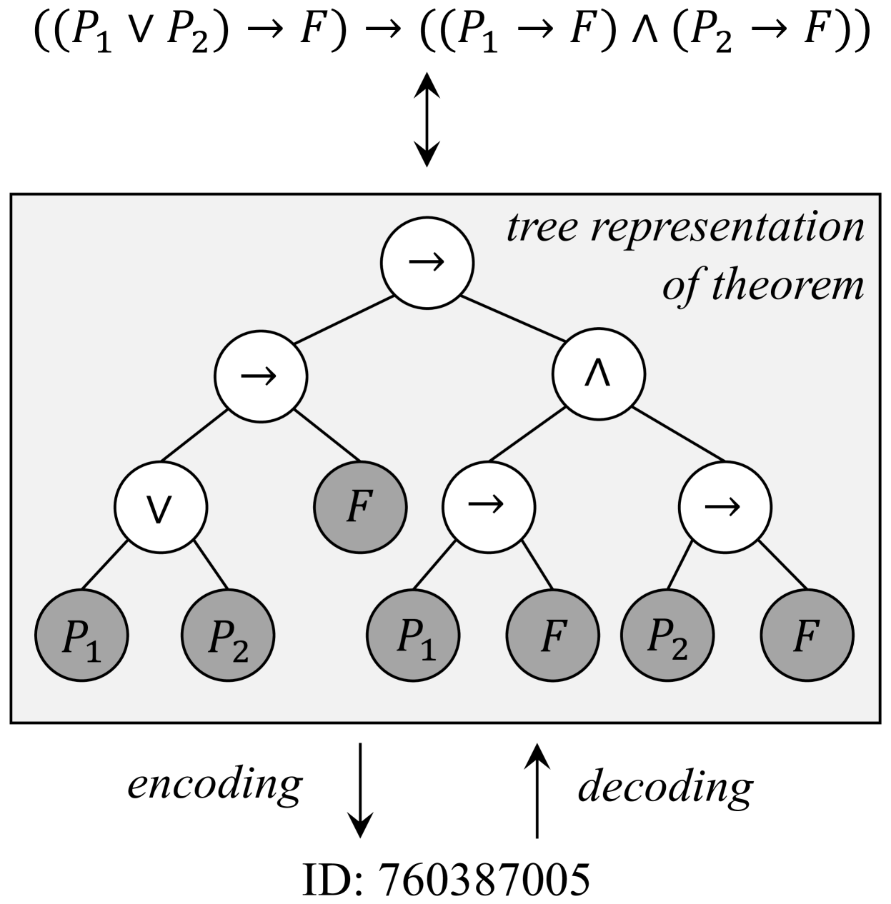The (recursive order (2 - 5)) of the right child For a fixed upper bound $p$ for the number of atomic propositions, we establish a bijection between the natural numbers and the set of propositional logic formulas. The counting can be made efficient using the Catalan Numbers Atkinson and Sack (1992). Figure 3 gives an example of mapping between propositions and natural numbers. Details about the encoding and decoding algorithms are provided in Appendix B. <details> <summary>x4.png Details</summary>  ### Visual Description ## Tree Diagram: Logical Theorem Representation ### Overview The image depicts a tree structure representing a logical theorem. The tree illustrates the decomposition of the logical expression `((P₁ ∨ P₂) → F)` into its constituent components, showing equivalence to `((P₁ → F) ∧ (P₂ → F))`. Arrows indicate hierarchical relationships, and nodes are labeled with logical operators (∨, →, ∧) and propositions (P₁, P₂, F). An encoding/decoding process is referenced via ID: 760387005. ### Components/Axes - **Root Node**: `(P₁ ∨ P₂) → F` - **Left Subtree**: - Node: `(P₁ → F) ∧ (P₂ → F)` - Branches: - `(P₁ → F)` → Leaves: `P₁`, `F` - `(P₂ → F)` → Leaves: `P₂`, `F` - **Right Subtree**: - Node: `(P₁ → F) ∧ (P₂ → F)` (identical to left subtree) - Branches: - `(P₁ → F)` → Leaves: `P₁`, `F` - `(P₂ → F)` → Leaves: `P₂`, `F` - **Encoding/Decoding Arrows**: - Downward arrow labeled "encoding" points to ID: 760387005. - Upward arrow labeled "decoding" points from ID: 760387005. ### Detailed Analysis - **Logical Structure**: - The root theorem `(P₁ ∨ P₂) → F` splits into two equivalent subtrees, each representing the conjunction `(P₁ → F) ∧ (P₂ → F)`. - Each subtree further decomposes into implications: - `P₁ → F` (if P₁ is true, then F must be true). - `P₂ → F` (if P₂ is true, then F must be true). - Leaves (`P₁`, `P₂`, `F`) represent atomic propositions. - **Encoding/Decoding**: - The ID `760387005` likely serves as a unique identifier for this theorem’s encoded representation. - The bidirectional arrows suggest a reversible process between the theorem’s logical form and its encoded ID. ### Key Observations 1. **Symmetry**: Both subtrees under the root are identical, emphasizing the equivalence of `(P₁ ∨ P₂) → F` and `(P₁ → F) ∧ (P₂ → F)`. 2. **Atomic Propositions**: `P₁`, `P₂`, and `F` are terminal nodes, indicating they are foundational assumptions or variables. 3. **Encoding ID**: The ID `760387005` is centrally positioned, linking the logical structure to a computational or formal representation. ### Interpretation This diagram demonstrates a fundamental logical equivalence in propositional logic: - **Theorem**: `(P₁ ∨ P₂) → F` is logically equivalent to `(P₁ → F) ∧ (P₂ → F)`. - This means "If either P₁ or P₂ is true, then F must be true" is equivalent to "P₁ implies F **and** P₂ implies F." - **Encoding/Decoding**: The ID `760387005` suggests this theorem is part of a formal system (e.g., automated theorem proving, knowledge representation). The encoding process translates the logical structure into a machine-readable format, while decoding reverses this. - **Significance**: The tree visually reinforces the decomposition of complex logical statements into simpler, verifiable components, aiding in proof construction or algorithmic verification. No numerical data or trends are present; the focus is on logical relationships and structural representation. </details> Figure 3: An illustration of the bijection between a proposition and a natural number, where gray nodes are leaf nodes. ID is computed using Algorithm 1 with $n=6$ and $p=2$ in this case. 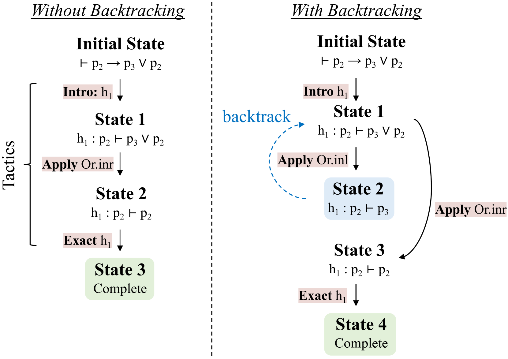Proof Generation. Given a randomly sampled theorem, the proof of the theorem is constructed using the focusing method with polarization McLaughlin and Pfenning (2009); Liang and Miller (2009); Pfenning (2017). Proof search is divided into two stages: inversion and chaining. The inversion phase mechanically breaks down negative connectives (e.g. implications) in the goal and positive connectives (e.g. disjunctions) in the premises. After inversion, chaining will pick an implication in the premise or show one of the disjuncts in the conclusion, with backtracking. The proof search procedure terminates when the same atomic proposition appears in both the premise and the conclusion. An example of proofs with trial-and-error information (backtracking) and with trial-and-error information removed are shown in Figure 4. Once proofs are generated, we use them to fine-tune models and start the proof search on the test set. The polarization of the connectives affects the behavior of the inversion and the search procedure. We choose to uniformly polarize conjunctions that occur negatively (e.g. on the right-hand side of an arrow) as negative and polarize conjunctions that occur positively (e.g. on the left-hand side of an arrow) as positive. Atomic propositions are assigned polarities based on the connective that they first appear under. To improve the runtime of the search procedure, we make an additional assumption that once an implication is picked, the implication cannot be used to show its premise. In theory, this introduces incompleteness into the search procedure, but it only affects 1 theorem out of around 1000 provable theorems randomly sampled. ### 3.2 Construction of Training and Test Sets In this section, we explain how we construct the datasets for training and evaluation. We want to avoid training and testing on similar data. In order to test the model performance on harder out-of-distribution (OOD) tasks, we need to ensure that the lengths of the proofs in the training data are shorter than the lengths of the proofs in the test data. Given PropL, we fix the number of internal nodes in the theorem statement to be 16 (explained in the dataset generation section). We then uniformly randomly sample 200,000 theorems from PropL, which can be achieved by using the integer-theorem bijection as explained before. Our method ensures that the theorems we study in this paper are representative of the propositional logic theorems in general. We first apply our deterministic algorithms to generate the proofs of the 200,000 theorems, and then remove the trial-and-error information of those proofs. We get a word-length distribution of those proofs without trial-and-error information. Next, to ensure the diversity of the trial-and-error information, we randomly select propositions to focus on during the chaining phase of the proof search, and then generate 10 different proofs with backtracking. By using the average length of the 10 different proofs, we have another word length distribution of proofs with trial-and-error information. We then split the 200,000 theorems into training and test sets based on both of the word length distributions mentioned above. The word lengths of the proofs of the training data theorems fall within the lower 0.66 quantile of the two distributions of the word length of all the proofs of the 200,000 theorems (109,887 in total). The word lengths of the in-distribution test set also fall in that category (1000 in total). The word lengths of the proofs among the out-of-distribution test theorems are above 0.8 quantile (1000 total) of the two distributions of the word lengths of all the proofs of the 200,000 theorems. We note that the baseline model and TrialMaster are trained on proofs of the same set of theorems. <details> <summary>x5.png Details</summary>  ### Visual Description ## Diagram: Comparison of Proof Tactics with/Without Backtracking ### Overview The diagram illustrates two parallel proof processes: one without backtracking (left) and one with backtracking (right). Both processes start from the same initial state but diverge in their handling of logical operations and state transitions. The "With Backtracking" side includes a feedback loop, enabling revisiting previous states. --- ### Components/Axes - **Left Side (Without Backtracking)**: - **Initial State**: `p2 → p3 ∨ p2` - **Tactics**: - `Intro h1` → **State 1**: `h1 : p2 ∨ p3 ∨ p2` - `Apply Or.inr` → **State 2**: `h1 : p2 ∨ p2` - `Exact h1` → **State 3**: `Complete` - **Flow**: Linear progression from State 1 → State 2 → State 3. - **Right Side (With Backtracking)**: - **Initial State**: `p2 → p3 ∨ p2` (identical to left) - **Tactics**: - `Intro h1` → **State 1**: `h1 : p2 ∨ p3 ∨ p2` - `Apply Or.inl` → **State 2**: `h1 : p2 ∨ p3` - `Apply Or.inr` (backtrack) → **State 2** (revisited) - `Apply Or.inr` → **State 3**: `h1 : p2 ∨ p2` - `Exact h1` → **State 4**: `Complete` - **Flow**: Non-linear with a feedback loop from State 2 → State 1 via `Apply Or.inl`. --- ### Detailed Analysis #### Left Side (Without Backtracking) 1. **State 1**: Introduces hypothesis `h1` with disjunction `p2 ∨ p3 ∨ p2`. 2. **State 2**: Applies `Or.inr` (right disjunct) to simplify to `p2 ∨ p2`. 3. **State 3**: Finalizes with `Exact h1`, marking completion. #### Right Side (With Backtracking) 1. **State 1**: Same as left, but uses `Or.inl` (left disjunct) to transition to **State 2**: `h1 : p2 ∨ p3`. 2. **Backtracking**: From **State 2**, `Apply Or.inr` reverts to **State 1**, enabling exploration of alternative paths. 3. **State 3**: Reapplies `Or.inr` to simplify to `p2 ∨ p2`. 4. **State 4**: Finalizes with `Exact h1`, marked as complete. --- ### Key Observations 1. **Backtracking Mechanism**: The right diagram introduces a feedback loop (`Apply Or.inl` → **State 1**), allowing revisiting of earlier states. This is absent in the left diagram. 2. **State Labeling**: Final states differ (`State 3` vs. `State 4`), suggesting distinct proof paths. 3. **Tactic Usage**: - Left: Uses `Or.inr` once. - Right: Uses `Or.inl` and `Or.inr` with backtracking, leading to a different final state. --- ### Interpretation - **Purpose of Backtracking**: The right diagram demonstrates how backtracking enables exhaustive exploration of proof paths. By revisiting **State 1**, the process can test alternative disjuncts (`Or.inl` vs. `Or.inr`), potentially leading to a more robust or generalized proof. - **State Completeness**: Both paths terminate in a "Complete" state, but the right diagram’s additional state (`State 4`) implies a more complex or extended proof process. - **Logical Structure**: The use of `Or.inl`/`Or.inr` reflects handling of disjunctions in proof systems, where backtracking allows revisiting hypotheses to explore all possible cases. This diagram highlights the trade-off between simplicity (left) and flexibility (right) in proof construction, with backtracking enabling deeper exploration at the cost of increased complexity. </details> Figure 4: Two proofs for one propositional logic theorem with tactics and states in Lean. ## 4 Methodology ### 4.1 LLM Fine-Tuning We utilize the training set formed in PropL for training both TrialMaster and the tactic generator in the DFS system. The numbers of theorems used in the training and test datasets are presented in Table 1. LLM fine-tuning with trial-and-error. In our approach, we randomly select two out of the shortest five among the ten proofs with trial-and-error information for each theorem in the training set and utilize them to train TrialMaster. Refer to Figure 2(b) for a description of this training process. LLM fine-tuning in a DFS system. For the tactic generator of the DFS system, we employ the deterministic FPS algorithm to generate the proofs of the theorems in the training set. The trial-and-error information is removed from the proofs. The LLM is then fine-tuned on the proofs without trial-and-error information as the conventional methods do. Figure 2(a) illustrates the training process of the DFS system. Table 1: The scale of training and test split in our PropL dataset. | Training set In-dist. test set Out-of-dist. test set | 109,887 1,000 1,000 | | --- | --- | ### 4.2 Inference Inference method of model trained with trial-and-error. TrialMaster conducts inference on itself without any help from a backtracking system like DFS or BFS. It outputs two kinds of tactics: tactics in Lean and backtrack instructions. An example of a backtrack instruction would be like “no solution, return to state 2 [that leads to state 4]”, where state 4 is the current state. When TrialMaster is doing a proof search on the test set, it is prompted with all history paths, including previous tactics, states, the backtracking it made before, and the failed search path. It then outputs the entire proof path after. Nonetheless, we only utilize the first tactic in the output and employ Lean as a calculator to determine the next state, thereby ensuring the correctness of the state following the tactic. If the tactic outputted by TrialMaster is a backtrack instruction, it is then prompted with all the proof search history including the backtrack instruction and the state that the backtrack instruction says to return to. If that tactic is not a backtrack instruction, the tactic and the current state will be fed into Lean for producing the state after. TrialMaster is then prompted with the entire proof tree including the state that Lean calculated, and it should output a tactic again. This process is repeated until Lean identifies that the proof is complete or any Lean error occurs. We also note that TrialMaster only outputs one tactic at each state using greedy search. Inference method of the DFS system. There are two hyperparameters in the DFS system: temperature $t$ and the number of sampled tactics $N_{\text{sampled}}$ . The temperature $t$ decides the diversity of the model outputs. As $t$ increases, the outputs of the model become more varied. The second parameter determines how many tactics the tactic generator of the DFS system produces for a new proof state. During inference, the LLM in the DFS system produces $N_{\text{sampled}}$ of candidate tactics at each new state. For each proof state, the DFS only makes one inference. If any two of the generated tactics for the same state are the same, we remove one of them to ensure efficiency. We also remove the tactic suggestions that fail to follow the grammar of Lean. The system follows the depth-first order to keep trying untried tactics. If the system exhausts all the tactics for a given state but has not found a valid one, the system returns to the parent state and then keeps trying untried tactics for the parent state. The overview is presented in the Figure 2(a). To fully exploit the ability of the DFS system, we varied the parameters of it, such as temperature and the number of sampled tactics. We count how many times Lean has been called to check tactics for both the DFS system and TrialMaster during the inference stage. #### Why do we choose DFS over BFS? While the breadth-first-search (BFS) system is also popular for building neural provers in Automated Theorem Proving, we have opted for DFS as our baseline over BFS in the context of propositional logic theorem proving. This is due to the finite number (around 20) of tactics available at any step for the search process of intuitionistic propositional logic theorems, making DFS more efficient than BFS without compromising the success rate. ## 5 Evaluation ### 5.1 Experimental Setup Base LLM. We used Llama-2-7b-hf Touvron et al. (2023) as the backbone LLM for tactic generation. Models are trained on two A100 GPUs for a single epoch with batch size set to $4$ . Huggingface Wolf et al. (2019) is used for fine-tuning the models, and VLLM Kwon et al. (2023) is used for inference of the models for efficiency. The learning rate of all training processes is set to be $2\times 10^{-5}$ . Hyperparameters. In the experiment, we vary temperature $t$ from $\{0.3,0.7,1.2,1.5,2.0\}$ and number of sampled tactics $N_{\text{sampled}}$ from $\{2,5,10,15,20\}$ . We notice that in all experiments for temperature $t$ less than 1.5, there were only very few (less than 15) theorems that were still under search when the total steps for that search attempt reached 65. For $t$ higher than 1.5, $N_{\text{Lean}}$ starts to increase dramatically. At temperature 2 with $N_{\text{sampled}}$ =20, $N_{\text{Lean}}$ climbs up to 32,171 when the number of total steps reaches 65. Therefore, in our experiment, we set 65 as the search step limit to control time complexity. <details> <summary>x6.png Details</summary>  ### Visual Description ## Line Graph: Success Rate vs. Temperature ### Overview The image is a line graph comparing the **Success Rate** of two methods, **TrialMaster** and **DFS**, across varying **Temperature** values. The graph includes two data series: one represented by an orange square (TrialMaster) and another by a blue line with circular markers (DFS). The x-axis represents **Temperature** (ranging from 0 to 2), and the y-axis represents **Success Rate** (ranging from 0.6 to 1.0). Numerical values are annotated near specific data points. --- ### Components/Axes - **X-axis (Temperature)**: Labeled "Temperature" with a scale from 0 to 2.0, marked at intervals of 0.5. - **Y-axis (Success Rate)**: Labeled "Success Rate" with a scale from 0.6 to 1.0, marked at intervals of 0.1. - **Legend**: Located in the bottom-right corner, with: - **Orange square**: TrialMaster - **Blue line with circles**: DFS - **Data Points**: - **TrialMaster**: Single orange square at (0, 0.90). - **DFS**: Blue line with circles at (0.5, 0.75), (1.0, 0.82), (1.5, 0.83), and (2.0, 0.90). --- ### Detailed Analysis - **TrialMaster**: - **Data Point**: (0, 0.90) — Success Rate of 0.90 at Temperature 0. - **Trend**: No additional data points; only one value is plotted. - **DFS**: - **Data Points**: - (0.5, 0.75): Success Rate of 0.75 at Temperature 0.5. - (1.0, 0.82): Success Rate of 0.82 at Temperature 1.0. - (1.5, 0.83): Success Rate of 0.83 at Temperature 1.5. - (2.0, 0.90): Success Rate of 0.90 at Temperature 2.0. - **Trend**: A steady upward slope from 0.75 to 0.90 as Temperature increases. --- ### Key Observations 1. **TrialMaster** achieves the highest Success Rate (0.90) at Temperature 0, but no data is provided for higher temperatures. 2. **DFS** shows a consistent increase in Success Rate with rising Temperature, reaching 0.90 at Temperature 2.0. 3. The **orange square** (TrialMaster) is positioned at the top-left corner of the graph, while the **blue line** (DFS) spans the entire x-axis range. --- ### Interpretation - **TrialMaster** appears to perform optimally at **Temperature 0**, but its lack of data at higher temperatures limits conclusions about its behavior under varying conditions. - **DFS** demonstrates a **positive correlation** between Temperature and Success Rate, suggesting it may be more effective or adaptable at higher temperatures. - The **orange square** (TrialMaster) is an outlier in terms of data density, as it only has one data point, whereas DFS has multiple points showing a clear trend. - The graph implies that **DFS** might be preferable in scenarios where higher temperatures are expected, while **TrialMaster** could be optimal at lower temperatures. However, further data for TrialMaster at higher temperatures would be needed to confirm this. </details> (a) Temperature $t$ <details> <summary>x7.png Details</summary>  ### Visual Description ## Line Graph: Success Rate vs. Number of Sampled Tactics ### Overview The image is a line graph comparing the success rates of two methods, **TrialMaster** (red square) and **DFS** (blue line with circles), as a function of the number of sampled tactics. The x-axis represents the number of sampled tactics (0–20), and the y-axis represents success rate (0.6–1.0). The graph includes numerical annotations for data points and a legend for method identification. --- ### Components/Axes - **X-axis**: "# of Sampled Tactic" (0–20, integer increments). - **Y-axis**: "Success Rate" (0.6–1.0, decimal increments). - **Legend**: - Red square: **TrialMaster** (positioned at bottom-right). - Blue line with circles: **DFS** (positioned at bottom-right). - **Data Points**: - **TrialMaster**: Single red square at (0, 0.9) with value **17993**. - **DFS**: Blue line with circles at: - (3, 0.7) → **13167** - (5, 0.8) → **15462** - (10, 0.82) → **16844** - (15, 0.85) → **17047** - (20, 0.86) → **17432** --- ### Detailed Analysis 1. **TrialMaster**: - Only one data point at **x=0** (no sampled tactics). - Success rate: **0.9** (90%). - Numerical value: **17993** (likely a count or metric tied to success rate). 2. **DFS**: - Success rate increases with more sampled tactics: - At **x=3**: 0.7 (70%) → 13167 - At **x=5**: 0.8 (80%) → 15462 - At **x=10**: 0.82 (82%) → 16844 - At **x=15**: 0.85 (85%) → 17047 - At **x=20**: 0.86 (86%) → 17432 - Trend: Gradual upward slope, indicating improved performance with more tactics. --- ### Key Observations - **TrialMaster** achieves a high success rate (0.9) without sampling any tactics, but its performance is not evaluated beyond this point. - **DFS** shows a clear positive correlation between the number of sampled tactics and success rate, with incremental improvements as tactics increase. - The numerical values (e.g., 17993, 13167) suggest a secondary metric (e.g., total successes, trials, or another quantifiable outcome) tied to the success rate. --- ### Interpretation - **TrialMaster** may represent a method that achieves high success rates without requiring tactical sampling (e.g., a static or rule-based approach). However, its lack of data beyond x=0 limits conclusions about scalability. - **DFS** demonstrates that success improves with increased tactical exploration, suggesting it is better suited for dynamic or adaptive scenarios where sampling more tactics enhances outcomes. - The numerical values (e.g., 17993 vs. 17432) imply that TrialMaster’s absolute performance (e.g., total successes) is higher at x=0, but DFS catches up and surpasses it in relative success rate as tactics increase. - The graph highlights a trade-off: TrialMaster is efficient at zero effort, while DFS requires more work but scales better. --- ### Spatial Grounding & Trend Verification - **Legend**: Bottom-right corner, clearly labels methods with matching colors. - **TrialMaster**: Red square at (0, 0.9) aligns with legend. - **DFS**: Blue line with circles follows the x-axis from 3 to 20, with success rate increasing monotonically (verified by upward slope). - **Axis Markers**: Dotted gridlines at 0.6, 0.7, 0.8, 0.9, 1.0 for y-axis; 0, 5, 10, 15, 20 for x-axis. --- ### Content Details - **TrialMaster**: - Single data point: (0, 0.9) → 17993. - **DFS**: - Data points: (3, 0.7), (5, 0.8), (10, 0.82), (15, 0.85), (20, 0.86). - Numerical values: 13167, 15462, 16844, 17047, 17432. --- ### Notable Anomalies - **TrialMaster** lacks data beyond x=0, making it impossible to assess its performance at higher tactic counts. - **DFS** shows diminishing returns: The rate of improvement slows as tactics increase (e.g., 0.82 to 0.85 between x=10 and x=15, then 0.85 to 0.86 between x=15 and x=20). --- ### Final Notes The graph emphasizes the importance of tactical sampling for DFS, while TrialMaster’s static performance suggests it may be less adaptable. Further data for TrialMaster at higher tactic counts would clarify its scalability. </details> (b) Sampled Tactics $N_{\text{sampled}}$ <details> <summary>x8.png Details</summary>  ### Visual Description ## Bar Chart: Number of Lean Calls by Method ### Overview The chart compares the number of lean calls (in thousands) across four methods: TrialMaster and three variations of DFS (Dynamic Filtering System) with different parameters. The y-axis represents the count of lean calls, while the x-axis lists the methods. The tallest bar corresponds to the DFS method with t=1.8 and 10 tactics, indicating it generates the most lean calls. ### Components/Axes - **X-axis (Method)**: - TrialMaster (brown bar) - DFS (t=1.5, 20 tactic) (light yellow bar) - DFS (t=1.5, 10 tactic) (light blue bar) - DFS (t=1.8, 10 tactic) (teal bar) - **Y-axis (# of Lean Calls)**: - Scale: 0 to 30 (thousand), with increments of 10. - Labels: "0", "10", "20", "30". - **Legend**: - Positioned in the top-left corner, matching bar colors to method names. - Colors: - Brown: TrialMaster - Light yellow: DFS (t=1.5, 20 tactic) - Light blue: DFS (t=1.5, 10 tactic) - Teal: DFS (t=1.8, 10 tactic) ### Detailed Analysis - **TrialMaster**: - Bar height ≈ 18,000 lean calls. - Shortest bar, indicating the lowest lean call volume. - **DFS (t=1.5, 20 tactic)**: - Bar height ≈ 19,500 lean calls. - Slightly taller than TrialMaster. - **DFS (t=1.5, 10 tactic)**: - Bar height ≈ 19,500 lean calls. - Matches the previous DFS variant in height. - **DFS (t=1.8, 10 tactic)**: - Bar height ≈ 31,000 lean calls. - Tallest bar, nearly double the others. ### Key Observations 1. **Dominance of DFS (t=1.8, 10 tactic)**: This method generates significantly more lean calls (~31k) compared to others (~18–19.5k). 2. **Similarity in DFS Variants**: The two DFS methods with t=1.5 (20 and 10 tactics) produce nearly identical results. 3. **TrialMaster Underperformance**: TrialMaster lags behind all DFS variants by ~1,500–3,000 calls. ### Interpretation The data suggests that the DFS method with a higher threshold (t=1.8) and fewer tactics (10) is the most effective at generating lean calls, potentially due to stricter filtering or higher sensitivity. The similarity between DFS variants with t=1.5 implies that the number of tactics (10 vs. 20) has minimal impact when the threshold remains constant. TrialMaster’s lower performance may indicate inefficiency or design differences compared to DFS. The outlier (DFS t=1.8) warrants further investigation into why increased thresholds correlate with higher call volumes. 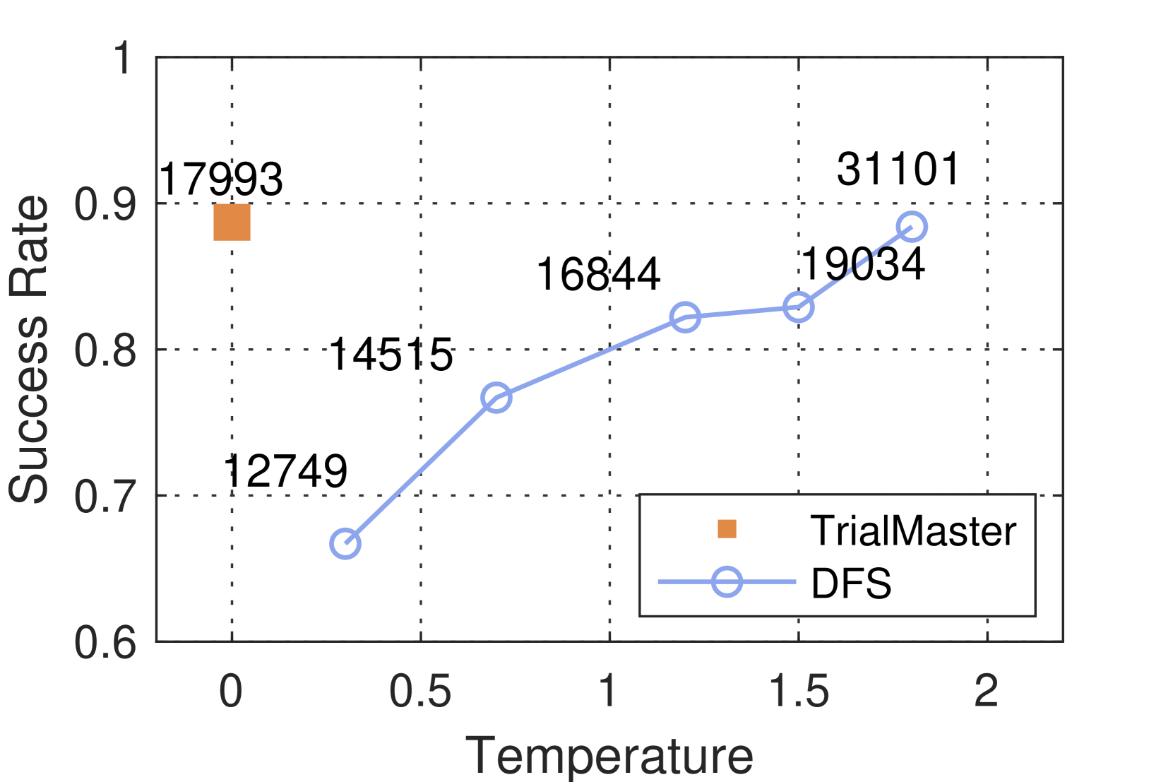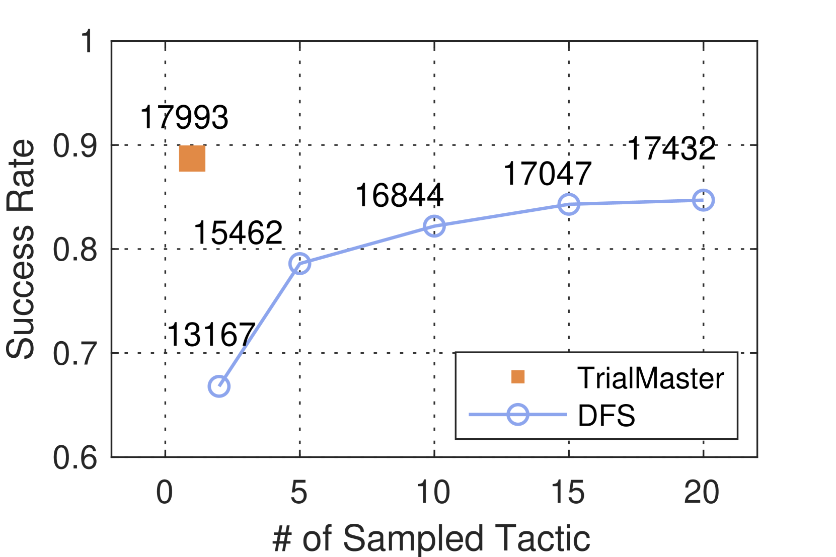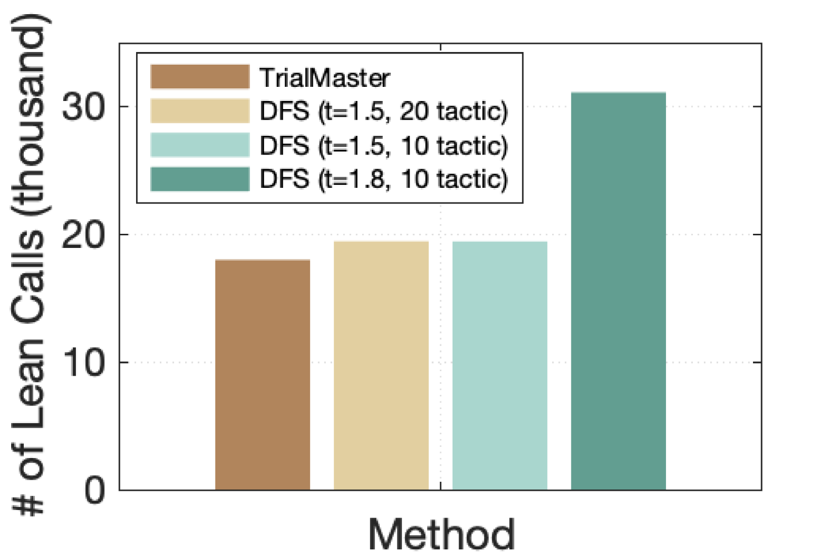</details> (c) Search Cost Figure 5: Experiment results on OOD task. (a) We fix $N_{\text{sampled}}=10$ to see the impact of temperature on the DFS system. (b) We fix $t=1.2$ to see the impact of the number of sampled tactics. The number of Lean calls is noted beside the marker. (c) Comparison of $N_{\text{Lean}}$ among our method and top 3 DFS systems with the highest success rate. In summary, training with trial-and-error achieves a higher success rate with a relatively lower search cost compared to the DFS systems. ### 5.2 Evaluation Metrics Proof search success rate. We use proof search success rate as our primary metric, which represents the ratio of successful searches by the model. A search attempt for a theorem is marked as successful if Lean outputs state “no goal, the proof is complete”, implying the theorem is effectively proved after applying a tactic produced by the model. For TrialMaster, a search attempt ends and fails immediately after one of the following conditions: 1) the word length of the proof tree with trial-and-error exceeds $1500$ (for the sake of context length of the model), or 2) the tactic produced by the model at any step induces a Lean error. For the conventional DFS system, a search attempt fails when one of the following conditions happens: 1) the word length of the proof tree without trial-and-error exceeds 1500, or 2) all tactics generated for the initial states have been explored and failed, or 3) the total search steps exceed 65 (see Section 5.1 for the choice of this value). We note that the 1500-word limit is stricter for our method since it produces entire proof paths including trial-and-error and thus would be easier to hit the limit. Search cost. We define a metric to assess the search cost—the total number of Lean calls for tactic checking during proof search for the entire test set, denoted as $N_{\text{Lean}}$ . Given the same proof search success rate, a lower $N_{\text{Lean}}$ indicates a more efficient system for proof search. Note that backtracking instructions from our method do not require applying Lean to check the state and, consequently do not add search cost. Table 2: Performance on in-distribution task. Both methods perform well for propositional logic. | DFS | $t=1.2$ | $N_{\text{sampled}}=2$ | 99.5% | | --- | --- | --- | --- | | $N_{\text{sampled}}=5$ | 99.9% | | | | $N_{\text{sampled}}=10$ | 99.6% | | | | $t=2.0$ | $N_{\text{sampled}}=2$ | 75.9% | | | $N_{\text{sampled}}=5$ | 97.3% | | | | $N_{\text{sampled}}=10$ | 99.0% | | | ### 5.3 Results and Analysis TrialMaster outperforms conventional DFS system. We begin by evaluating the methods of the in-distribution test set. Table 2 illustrates that both our method and the DFS system perform exceptionally well, achieving a success rate of nearly 100% in most configurations. This suggests that Llama-7b effectively masters in-distribution intuitionistic propositional logic theorems. Then, we compare the performance of the methods on the out-of-distribution task. The results are presented in Figure 5. Our method with trial-and-error significantly outperforms the DFS system across various hyperparameter configurations. Additionally, we observe that feeding more proofs without trial-and-error for LLM fine-tuning does not further improve the performance. Impact of hyperparameters in the DFS system. As shown in Figure 5, on the OOD task, although the success rate of the DFS system gets higher when we increase the temperature $t$ or the number of sampled tactics $N_{\text{sampled}}$ , the search cost (reflected by $N_{\text{Lean}}$ ) also goes up. Specifically, when we increase $N_{\text{sampled}}$ , the DFS system explores a larger pool of candidate tactics during the search, leading to a higher number of Lean calls. In contrast, our method does a greedy search to generate only one tactic for each new state. Likewise, as $t$ increases, the tactic generator of the DFS system tends to produce more diverse tactics at each proof state, improving the system’s performance but leading to higher search costs. Table 3: Ablation study: Comparison of TrialMaster and model trained without trial-and-error information on OOD task | TrialMaster Model - proof w/o t.a.e. | 88.7% 59.3 % | | --- | --- | TrialMaster achieves high success rates at lower search cost. For a direct comparison of search costs, we plot the $N_{\text{Lean}}$ values of our method alongside those of the top three DFS systems with the highest success rates among all the hyperparameters we experimented with, i.e., $t$ =1.5, $N_{\text{sampled}}$ =20 (87.2%), $t$ =1.5, $N_{\text{sampled}}$ = 10 (86.1%), and $t$ =1.8, $N_{\text{sampled}}$ =10 (88.4%). This comparison is illustrated in Figure 5(c). Notably, we observe that the DFS systems that closely approach our model’s performance exhibit significantly higher search costs. With $t$ =1.8, $N_{\text{sampled}}$ =10, $N_{\text{Lean}}$ of the DFS system, which has 0.3% lower success rate than our method, has reached 31,101, which is 72% higher than that of our method with trial-and-error. The high search cost makes the DFS system with high temperatures unfavorable. These results demonstrate that training with trial-and-error produces higher-quality tactics, achieving a higher success rate with relatively lower search cost. Model learns backtracking capability from trial-and-error data. In the experiments, we find out that our TrialMaster successfully acquires the backtracking capability from proofs with trial-and-error information. This is evidenced by the fact that during TrialMaster ’s proof search for theorems in the test set, all backtracking instructions produced by the LLM adhere to the correct format and point to existing state numbers. Including failed search paths helps TrialMaster to learn. The following experiment shows that adding failed search paths to the training data for TrialMaster results in an overall gain. In this experiment, the model is only trained to learn the correct search paths and the backtracking instructions. The model is not trained to learn the failed search paths (we don’t compute the loss for the failed search paths during the training stage in this case). The proof success rate in this case is 75.6%, which is lower than TrialMaster ’s proof success rate of 88.7%. The $N_{\text{Lean}}$ for the model is 13,600, which is lower than that of TrialMaster. This is expected since the model does not learn to predict failed search paths. Our explanation for why TrialMaster has a higher proof search success rate than the model trained in the previously mentioned experiment is that the failed search paths also contribute to improving the proof search success rate of the model. TrialMaster strategically tried some potentially failed search paths to gain a more comprehensive view of the problem, which then led to the correct search paths. ### 5.4 Ablation Study To evaluate the effectiveness of training with trial-and-error, we craft an ablated version of our method where the LLM is fined-tuned with data of the correct path only and do inference in the same way as our method (i.e., producing one tactic at a time and applying Lean for state checking). We denote the ablated version as Model - proof w/o t.a.e.. For both methods, we mark the search attempt as failed if the tactic induces a Lean error, or the search exceeds the 1500-word limit. The result is shown in the Table 3. The difference between the success rates of the two models is $29.4\$ , which is significant. This clearly shows that failed search states and trial-and-error information tremendously enhance the model’s capability to solve theorem-proving tasks. Table 4: Comparison of models trained on different lengths of proofs with trial-and-error on OOD task. | Model - short proof w/ t.a.e. Model - long proof w/ t.a.e. | 88.7% 72.4 % | | --- | --- | ### 5.5 Exploratory Study: Effect of Training Proof Length on Model Performance Since the FPS algorithm of PropL dataset can generate multiple proofs with variable length, we conduct an exploratory study to assess the impact of proof length on model performance. We fine-tune two models using proofs with different lengths of trial-and-error information. For the first model, which is our TrialMaster, the training data is derived by randomly selecting two out of the shortest four proofs from the ten available proofs for each theorem in PropL. We denote it as Model - short proof w/ t.a.e. In contrast, the training data of the second model is formed by randomly selecting two proofs from the ten available for each theorem, irrespective of their lengths. We denote it as Model - long proof w/ t.a.e. For both models, we use greedy search to let them generate one tactic for each state. We evaluate the models on our 1000 OOD test set. The results are shown in the Table 4. A higher success rate is observed in the model trained with shorter proofs. This can be attributed to the fact that as the proof with trial-and-error information becomes longer, there is too much trial-and-error information that may detrimentally affect the model’s performance, as too many failed search paths may lower the quality of the training data. ## 6 Conclusion and Future Work In this paper, we study Automated Theorem Proving in formalized environments. We create a complete, scalable, and representative dataset of intuitionistic propositional logic theorems in Lean. We demonstrate that leveraging information from failed search states and backtracking not only teaches models how to backtrack effectively, but also helps in developing better tactics than those generated by models trained without access to backtracking insights. We release our datasets on GitHub and Huggingface. PropL dataset is available at https://huggingface.co/datasets/KomeijiForce/PropL. Model weights are available at https://huggingface.co/KomeijiForce/llama-2-7b-propositional-logic-prover. Generation codes for theorems and proofs are available at https://github.com/ucsd-atp/PropL. A natural extension of our research involves investigating whether trial-and-error information is beneficial for more general mathematical theorem-proving settings. Exploring this avenue could provide valuable insights into the effectiveness of our approach across broader mathematical domains. ## Limitations One limitation of our study is that some proof attempts are forced to stop due to the prompt exceeding the context length of 1500 tokens. This constraint may potentially influence our results by truncating the available information during the proof search process. Furthermore, our method was not evaluated on general mathematical theorems. This limitation arises from both the scarcity of proofs containing trial-and-error information in current math libraries and the intrinsic challenges associated with producing proofs, whether with or without backtracking, for general mathematical theorems in a formalized setting. Automated theorem proving with LLMs is an emerging area in machine learning. There is still a lack of baselines on LLMs to compare with our method. We establish a fundamental baseline, but we still need accumulative work to provide methods for comparison. ## Ethical Consideration Our work learns large language models to automatically prove propositional logic theorems, which generally does not raise ethical concerns. ## Acknowledgments This work is supported by the National Science Foundation under grants CCF-1955457 and CCF-2220892. This work is also sponsored in part by NSF CAREER Award 2239440, NSF Proto-OKN Award 2333790, as well as generous gifts from Google, Adobe, and Teradata. ## References - Atkinson and Sack (1992) Michael D Atkinson and J-R Sack. 1992. Generating binary trees at random. Information Processing Letters, 41(1):21–23. - Bansal et al. (2019) Kshitij Bansal, Christian Szegedy, Markus N Rabe, Sarah M Loos, and Viktor Toman. 2019. Learning to reason in large theories without imitation. arXiv preprint arXiv:1905.10501. - Barras et al. (1997) Bruno Barras, Samuel Boutin, Cristina Cornes, Judicaël Courant, Jean-Christophe Filliatre, Eduardo Gimenez, Hugo Herbelin, Gerard Huet, Cesar Munoz, Chetan Murthy, et al. 1997. The Coq proof assistant reference manual: Version 6.1. Ph.D. thesis, Inria. - Besta et al. (2023) Maciej Besta, Nils Blach, Ales Kubicek, Robert Gerstenberger, Lukas Gianinazzi, Joanna Gajda, Tomasz Lehmann, Michal Podstawski, Hubert Niewiadomski, Piotr Nyczyk, et al. 2023. Graph of thoughts: Solving elaborate problems with large language models. arXiv preprint arXiv:2308.09687. - Chang and Lee (2014) Chin-Liang Chang and Richard Char-Tung Lee. 2014. Symbolic logic and mechanical theorem proving. Academic press. - Chen et al. (2024) Sijia Chen, Baochun Li, and Di Niu. 2024. Boosting of thoughts: Trial-and-error problem solving with large language models. In The Twelfth International Conference on Learning Representations. - Chu et al. (2023) Zheng Chu, Jingchang Chen, Qianglong Chen, Weijiang Yu, Tao He, Haotian Wang, Weihua Peng, Ming Liu, Bing Qin, and Ting Liu. 2023. A survey of chain of thought reasoning: Advances, frontiers and future. arXiv preprint arXiv:2309.15402. - Clocksin and Mellish (2003) William F Clocksin and Christopher S Mellish. 2003. Programming in PROLOG. Springer Science & Business Media. - Crevier (1993) Daniel Crevier. 1993. AI: the tumultuous history of the search for artificial intelligence. Basic Books, Inc. - Davies et al. (2021) Alex Davies, Petar Veličković, Lars Buesing, Sam Blackwell, Daniel Zheng, Nenad Tomašev, Richard Tanburn, Peter Battaglia, Charles Blundell, András Juhász, et al. 2021. Advancing mathematics by guiding human intuition with AI. Nature, 600(7887):70–74. - Davis (2001) Martin Davis. 2001. The early history of automated deduction. Handbook of automated reasoning, 1:3–15. - de Moura et al. (2015) Leonardo de Moura, Soonho Kong, Jeremy Avigad, Floris Van Doorn, and Jakob von Raumer. 2015. The lean theorem prover (system description). In Automated Deduction-CADE-25: 25th International Conference on Automated Deduction, Berlin, Germany, August 1-7, 2015, Proceedings 25, pages 378–388. Springer. - First et al. (2023) Emily First, Markus Rabe, Talia Ringer, and Yuriy Brun. 2023. Baldur: Whole-proof generation and repair with large language models. In Proceedings of the 31st ACM Joint European Software Engineering Conference and Symposium on the Foundations of Software Engineering, pages 1229–1241. - Fu et al. (2022) Yao Fu, Hao Peng, Ashish Sabharwal, Peter Clark, and Tushar Khot. 2022. Complexity-based prompting for multi-step reasoning. arXiv preprint arXiv:2210.00720. - Gilmore (1960) P. C. Gilmore. 1960. A proof method for quantification theory: Its justification and realization. IBM Journal of Research and Development, 4(1):28–35. - Han et al. (2021) Jesse Michael Han, Jason Rute, Yuhuai Wu, Edward W Ayers, and Stanislas Polu. 2021. Proof artifact co-training for theorem proving with language models. arXiv preprint arXiv:2102.06203. - Holden and Korovin (2021) Edvard K Holden and Konstantin Korovin. 2021. Heterogeneous heuristic optimisation and scheduling for first-order theorem proving. In International Conference on Intelligent Computer Mathematics, pages 107–123. Springer. - Irving et al. (2016) Geoffrey Irving, Christian Szegedy, Alexander A Alemi, Niklas Eén, François Chollet, and Josef Urban. 2016. Deepmath-deep sequence models for premise selection. Advances in neural information processing systems, 29. - Jiang et al. (2022) Albert Q Jiang, Sean Welleck, Jin Peng Zhou, Wenda Li, Jiacheng Liu, Mateja Jamnik, Timothée Lacroix, Yuhuai Wu, and Guillaume Lample. 2022. Draft, sketch, and prove: Guiding formal theorem provers with informal proofs. arXiv preprint arXiv:2210.12283. - Kusumoto et al. (2018) Mitsuru Kusumoto, Keisuke Yahata, and Masahiro Sakai. 2018. Automated theorem proving in intuitionistic propositional logic by deep reinforcement learning. arXiv preprint arXiv:1811.00796. - Kwon et al. (2023) Woosuk Kwon, Zhuohan Li, Siyuan Zhuang, Ying Sheng, Lianmin Zheng, Cody Hao Yu, Joseph Gonzalez, Hao Zhang, and Ion Stoica. 2023. Efficient memory management for large language model serving with pagedattention. In Proceedings of the 29th Symposium on Operating Systems Principles, pages 611–626. - Lample et al. (2022) Guillaume Lample, Timothee Lacroix, Marie-Anne Lachaux, Aurelien Rodriguez, Amaury Hayat, Thibaut Lavril, Gabriel Ebner, and Xavier Martinet. 2022. Hypertree proof search for neural theorem proving. Advances in Neural Information Processing Systems, 35:26337–26349. - Liang and Miller (2009) Chuck C. Liang and Dale Miller. 2009. Focusing and polarization in linear, intuitionistic, and classical logics. Theor. Comput. Sci., 410(46):4747–4768. - McCorduck (2004) Pamela McCorduck. 2004. Machines Who Think (2Nd Ed.). A. K. Peters. - McLaughlin and Pfenning (2009) Sean McLaughlin and Frank Pfenning. 2009. Efficient intuitionistic theorem proving with the polarized inverse method. In Automated Deduction - CADE-22, 22nd International Conference on Automated Deduction, Montreal, Canada, August 2-7, 2009. Proceedings, volume 5663 of Lecture Notes in Computer Science, pages 230–244. Springer. - Megill and Wheeler (2019) Norman Megill and David A Wheeler. 2019. Metamath: a computer language for mathematical proofs. Lulu. com. - Mikuła et al. (2023) Maciej Mikuła, Szymon Antoniak, Szymon Tworkowski, Albert Qiaochu Jiang, Jin Peng Zhou, Christian Szegedy, Łukasz Kuciński, Piotr Miłoś, and Yuhuai Wu. 2023. Magnushammer: A transformer-based approach to premise selection. arXiv preprint arXiv:2303.04488. - Nawaz et al. (2019) M Saqib Nawaz, Moin Malik, Yi Li, Meng Sun, and M Lali. 2019. A survey on theorem provers in formal methods. arXiv preprint arXiv:1912.03028. - Nipkow et al. (2002) Tobias Nipkow, Markus Wenzel, and Lawrence C Paulson. 2002. Isabelle/HOL: a proof assistant for higher-order logic. Springer. - Pfenning (2017) Frank Pfenning. 2017. Lecture notes on focusing. - Polu and Sutskever (2020) Stanislas Polu and Ilya Sutskever. 2020. Generative language modeling for automated theorem proving. arXiv preprint arXiv:2009.03393. - Rabe et al. (2020) Markus N Rabe, Dennis Lee, Kshitij Bansal, and Christian Szegedy. 2020. Mathematical reasoning via self-supervised skip-tree training. arXiv preprint arXiv:2006.04757. - Robinson (1965) John Alan Robinson. 1965. A machine-oriented logic based on the resolution principle. Journal of the ACM (JACM), 12(1):23–41. - Russell and Norvig (2010) Stuart J Russell and Peter Norvig. 2010. Artificial intelligence a modern approach. London. - Sekiyama et al. (2017) Taro Sekiyama, Akifumi Imanishi, and Kohei Suenaga. 2017. Towards proof synthesis guided by neural machine translation for intuitionistic propositional logic. corr abs/1706.06462 (2017). arXiv preprint arXiv:1706.06462. - Sekiyama and Suenaga (2018) Taro Sekiyama and Kohei Suenaga. 2018. Automated proof synthesis for propositional logic with deep neural networks. arXiv preprint arXiv:1805.11799. - Stanley (2015) Richard P Stanley. 2015. Catalan numbers. Cambridge University Press. - Thakur et al. (2023) Amitayush Thakur, Yeming Wen, and Swarat Chaudhuri. 2023. A language-agent approach to formal theorem-proving. arXiv preprint arXiv:2310.04353. - Touvron et al. (2023) Hugo Touvron, Louis Martin, Kevin Stone, Peter Albert, Amjad Almahairi, Yasmine Babaei, Nikolay Bashlykov, Soumya Batra, Prajjwal Bhargava, Shruti Bhosale, et al. 2023. Llama 2: Open foundation and fine-tuned chat models. arXiv preprint arXiv:2307.09288. - Wagner (2021) Adam Zsolt Wagner. 2021. Constructions in combinatorics via neural networks. arXiv preprint arXiv:2104.14516. - Wang et al. (2023) Haiming Wang, Ye Yuan, Zhengying Liu, Jianhao Shen, Yichun Yin, Jing Xiong, Enze Xie, Han Shi, Yujun Li, Lin Li, et al. 2023. Dt-solver: Automated theorem proving with dynamic-tree sampling guided by proof-level value function. In Proceedings of the 61st Annual Meeting of the Association for Computational Linguistics (Volume 1: Long Papers), pages 12632–12646. - Wang and Deng (2020) Mingzhe Wang and Jia Deng. 2020. Learning to prove theorems by learning to generate theorems. Advances in Neural Information Processing Systems, 33:18146–18157. - Wang et al. (2017) Mingzhe Wang, Yihe Tang, Jian Wang, and Jia Deng. 2017. Premise selection for theorem proving by deep graph embedding. Advances in neural information processing systems, 30. - Wang et al. (2022) Xuezhi Wang, Jason Wei, Dale Schuurmans, Quoc Le, Ed Chi, Sharan Narang, Aakanksha Chowdhery, and Denny Zhou. 2022. Self-consistency improves chain of thought reasoning in language models. arXiv preprint arXiv:2203.11171. - Wei et al. (2022) Jason Wei, Xuezhi Wang, Dale Schuurmans, Maarten Bosma, Fei Xia, Ed Chi, Quoc V Le, Denny Zhou, et al. 2022. Chain-of-thought prompting elicits reasoning in large language models. Advances in Neural Information Processing Systems, 35:24824–24837. - Welleck et al. (2021) Sean Welleck, Jiacheng Liu, Ronan Le Bras, Hannaneh Hajishirzi, Yejin Choi, and Kyunghyun Cho. 2021. Naturalproofs: Mathematical theorem proving in natural language. arXiv preprint arXiv:2104.01112. - Wolf et al. (2019) Thomas Wolf, Lysandre Debut, Victor Sanh, Julien Chaumond, Clement Delangue, Anthony Moi, Pierric Cistac, Tim Rault, Rémi Louf, Morgan Funtowicz, et al. 2019. Huggingface’s transformers: State-of-the-art natural language processing. arXiv preprint arXiv:1910.03771. - Wu et al. (2021) Minchao Wu, Michael Norrish, Christian Walder, and Amir Dezfouli. 2021. Tacticzero: Learning to prove theorems from scratch with deep reinforcement learning. Advances in Neural Information Processing Systems, 34:9330–9342. - Yang et al. (2023) Kaiyu Yang, Aidan M Swope, Alex Gu, Rahul Chalamala, Peiyang Song, Shixing Yu, Saad Godil, Ryan Prenger, and Anima Anandkumar. 2023. LeanDojo: Theorem Proving with Retrieval-Augmented Language Models. arXiv preprint arXiv:2306.15626. - Yao et al. (2023) Shunyu Yao, Dian Yu, Jeffrey Zhao, Izhak Shafran, Thomas L Griffiths, Yuan Cao, and Karthik Narasimhan. 2023. Tree of thoughts: Deliberate problem solving with large language models. arXiv preprint arXiv:2305.10601. - Yu et al. (2023) Fei Yu, Hongbo Zhang, and Benyou Wang. 2023. Nature language reasoning, a survey. arXiv preprint arXiv:2303.14725. - Zheng et al. (2023) Chuanyang Zheng, Haiming Wang, Enze Xie, Zhengying Liu, Jiankai Sun, Huajian Xin, Jianhao Shen, Zhenguo Li, and Yu Li. 2023. Lyra: Orchestrating dual correction in automated theorem proving. arXiv preprint arXiv:2309.15806. - Zhou et al. (2022) Denny Zhou, Nathanael Schärli, Le Hou, Jason Wei, Nathan Scales, Xuezhi Wang, Dale Schuurmans, Claire Cui, Olivier Bousquet, Quoc Le, et al. 2022. Least-to-most prompting enables complex reasoning in large language models. arXiv preprint arXiv:2205.10625. ## Appendix A Inference Rules for Intuitionistic Propositional Logic Figure 6 shows the inference rules for intuitionistic propositional logic. Rules relate sequents of the form $\Gamma\vdash A$ , where $\Gamma$ is an unordered list of assumptions. A derivation is constructed from the axiom (Assumption) using the derivation rules until $\Gamma$ is empty. For example, the ( $\to$ -I) rule says that from a derivation of $\Gamma\vdash B$ under the assumption of $\Gamma,A$ , we can get a derivation of $\Gamma\vdash A\to B$ . The ( $\to$ -E) rule says that from a derivation of $\Gamma\vdash A\to B$ and a derivation of $\Gamma\vdash A$ we can derive $\Gamma\vdash B$ . Γ, A ⊢A (Assumption) Γ⊢T (T-I) Γ⊢FΓ⊢A (F-E) Γ⊢A Γ⊢BΓ⊢A ∧B ( $\land$ -I) Γ⊢A ∧BΓ⊢A ( $\land$ -E1) Γ⊢A ∧BΓ⊢B ( $\land$ -E2) Γ⊢AΓ⊢A ∨B ( $\lor$ -I1) Γ⊢BΓ⊢A ∨B ( $\lor$ -I2) Γ⊢A ∨B Γ, A ⊢C Γ, B ⊢CΓ⊢C ( $\lor$ -E) Γ, A ⊢BΓ⊢A →B ( $\to$ -I) Γ⊢A →B Γ⊢A Γ⊢B ( $\to$ -E) Figure 6: Natural Deduction Rules for Intuitionistic Propositional Logic Here are an example derivation. $\texttt{p1}\to\texttt{p1}\lor\texttt{p2}$ . $$ \vdash\texttt{p1}\to\texttt{p1}\lor\texttt{p2}\texttt{p1}\vdash\texttt{p1}\lor \texttt{p2}\texttt{p1}\vdash\texttt{p1} $$ ## Appendix B Uniformly Distributed Data Explanation In this section, we discuss the uniform characteristics of our dataset, particularly emphasizing the one-to-one mapping between propositions and natural numbers. This bijection allows us to simply sample from the natural numbers to ensure the dataset exhibits uniformity. Algorithm 1 Encoding 1: A tree $\mathcal{T}$ representing a proposition, with $n$ indicating the number of internal nodes and $p$ representing the number of atomic propositions 2: Output a natural number 3: return $3^{n}(p+2)^{n+1}$ $\times$ ShapeNumber ( $\mathcal{T}$ ) $+$ AssignmentNumber ( $\mathcal{T}$ ) 4: function ShapeNumber ( $\mathcal{T}$ ) 5: if $\mathcal{T}$ is a single node then return $0 0$ 6: end if 7: $\mathcal{T}_{l},\mathcal{T}_{r}\leftarrow$ left and right sub-trees of $\mathcal{T}$ 8: $n_{l},n_{r}\leftarrow$ number of internal nodes in $\mathcal{T}_{l},\mathcal{T}_{r}$ $\triangleright$ Total $n_{r}+n_{l}+1$ internal nodes 9: return $\sum_{i=1}^{n_{l}}C_{i-1}C_{n_{l}+n_{r}+1-i}$ $+$ $C_{n_{r}}$ $\times$ ShapeNumber ( $\mathcal{T}_{l}$ ) $+$ ShapeNumber ( $\mathcal{T}_{r}$ ) 10: end function 11: function AssignmentNumber ( $\mathcal{T}$ ) 12: $N\leftarrow$ NodeNumber (root node of $\mathcal{T}$ ) 13: if $\mathcal{T}$ is a single node then return $N$ 14: end if 15: $\mathcal{T}_{l},\mathcal{T}_{r}\leftarrow$ left and right sub-trees of $\mathcal{T}$ 16: $n_{r}\leftarrow$ number of internal nodes in $\mathcal{T}_{r}$ 17: $A_{r}\leftarrow 3^{n_{r}}(p+2)^{n_{r}+1}$ $\triangleright$ Compute all possible assignments in the right sub-tree 18: return $3A_{r}$ $\times$ AssignmentNumber ( $\mathcal{T}_{l}$ ) $+$ $A_{r}$ $\times$ $N$ $+$ AssignmentNumber ( $\mathcal{T}_{r}$ ) 19: end function 20: function NodeNumber ( $\mathcal{N}$ ) 21: switch $\mathcal{N}$ 22: case $\land$ or $T$ : return 0 23: case $\lor$ or $F$ : return 1 24: case $\rightarrow$ : return 2 25: case $P_{i}$ : return $i+1$ $\triangleright$ $1\leq i\leq p$ 26: end function ### B.1 Catalan Number The Catalan number $C_{n}$ is applicable for counting full binary trees that consist of $n+1$ leaf nodes, corresponding to exactly $n$ internal nodes Stanley (2015). Additionally, it can be calculated through recursion as shown: $$ C_{n}=\sum_{i=1}^{n}C_{i-1}C_{n-i}. $$ The first Catalan numbers for $n=0,1,2,3,4$ are $1,1,2,5,14$ . A concise interpretation of this recursion is as follows: it involves counting the number of internal nodes in the left sub-tree, amounting to $i-1$ , and then in the right sub-tree, amounting to $n-i$ , for each of the $n$ scenarios in computing $C_{n}$ . Algorithm 2 Decoding 1: A natural number ID, with $n$ indicating the number of internal nodes and $p$ representing the number of atomic propositions 2: Output a proposition tree 3: quotient, remainder $\leftarrow$ DivMod (ID, $3^{n}(p+2)^{n+1}$ ) 4: $S\leftarrow$ TreeShape (quotient, $n$ ) 5: $A\leftarrow$ TreeAssignment ( $S$ , remainder) 6: return a tree with shape $S$ and assignment $A$ 7: function TreeShape ( $N$ , $n$ ) 8: if $n$ is $0 0$ then return a single node 9: end if 10: $n_{l}\leftarrow\max(\{k|\sum_{i=1}^{k}C_{i-1}C_{n-i}\leq N\}\cup\{0\})$ 11: $n_{r}\leftarrow n-n_{l}-1$ 12: remaining $\leftarrow N-\sum_{i=1}^{n_{l}}C_{i-1}C_{n-i}$ 13: $N_{l},N_{r}\leftarrow$ DivMod (remaining, $C_{n_{r}}$ ) 14: return a tree with left and right sub-trees shaped by TreeShape ( $N_{l}$ , $n_{l}$ ) and TreeShape ( $N_{r}$ , $n_{r}$ ), respectively 15: end function 16: function TreeAssignment ( $S$ , $N$ ) 17: Perform an inorder traversal of the tree with shape $S$ . For each leaf node, interpret it as a digit in base $p+2$ , and for each internal node, interpret it as a digit in base 3. Compute the assignment that gives $N$ by utilizing the NodeNumber function introduced in Algorithm 1 18: end function ### B.2 Bijection between Propositions and Natural Numbers As depicted in Figure 3, every proposition corresponds to a unique tree representation. Consequently, it only requires the identification of a bijection between full binary trees and natural numbers. For every full binary tree possessing $n$ internal nodes and $p$ atomic propositions, there exist | | $\displaystyle 3^{\#\text{internal node}}(p+2)^{\#\text{leaf node}}=3^{n}(p+2)^ {n+1}$ | | | --- | --- | --- | distinct cases. Observe that the choices available for internal nodes include conjunction ( $\land$ ), disjunction ( $\lor$ ), and implication ( $\rightarrow$ ); whereas for leaf nodes, the choices encompass true ( $T$ ), false ( $F$ ), and a set of propositions $P_{1},\ldots,P_{p}$ . This counting facilitates an efficient ranking of all full binary trees with $n$ internal nodes. This ranking process inherently establishes a bijection with the set of natural numbers, allowing for a clear correspondence between each full binary tree and a unique natural number. Consequently, this sets the stage for a detailed examination of two critical processes: encoding (see Algorithm 1), which involves mapping a proposition tree to a natural number, and decoding (see Algorithm 2), which entails mapping a natural number back to a corresponding proposition tree. Having established the bijection between full binary trees and natural numbers, it becomes apparent that uniformly sampling from the set of natural numbers will, in turn, result in a uniform sampling of full binary trees. The inclusion of the parameter $n$ in Algorithm 1 is not critical for the functionality of the algorithm as $n$ can be counted from $\mathcal{T}$ ; however, it is retained to denote that the most basic encoding and decoding approaches are designed for a fixed number of internal nodes $n$ . For example, ID 0 denotes different propositions depending on the specified value of $n$ . As a result, the decoding algorithm, as outlined in Algorithm 2, is specifically intended for uniformly generating proposition trees with a fixed $n$ . To achieve a uniformly distributed proposition tree from a set of trees with various $n$ , one might simply merge the rankings of fully binary trees with different $n$ , a task which can be performed with relative ease. This approach of merging can be similarly applied to trees with varying $p$ as well. Given the uncertainty surrounding the proof lengths when generating propositions, our approach involves uniform sampling for proposition selection. This selection is later refined by excluding propositions according to their proof lengths as computed by the proof generation algorithm. ## Appendix C Examples In Figure 7, we show an example Lean proof for a theorem in Figure 3. Lines preceded by ’–’ are comments solely for explanatory purposes. ⬇ variable (p1 p2 p3 p4 p5 : Prop) theorem : (((p1 ∨ p2) → False) → ((p1 → False) ∧ (p2 → False))) := by – Implications on the right can always be decomposed. – Introduce an assumption h1 that says ((p1 ∨ p2) → False) intro h1 – Now we want to show ((p1 → False) ∧ (p2 → False)) – Conjunctions on the right can always be decomposed. – We then need to show (p1 → False) and (p2 → False) separately. apply And. intro – We are showing (p1 → False). – Implications on the right can always be decomposed. – We introduce assumption h2 for p1. And we try to show False. intro h2 – We want to use the implication h1. So we show its premise. have h3 : (p1 ∨ p2) := by – Show the left disjunct. (The right adjunct leads to an TAE) apply Or. inl – One of the premise coincides with the conclusion. exact h2 – We have shown the premise of h1 (p1 ∨ p2), – we can now drive its conclusion (False), denoted by h4. let h4 := h1 h3 – False on the left can always be used. apply False. elim h4 – We have shown (p1 → False) and now we show (p2 → False). – Implications on the right can always be decomposed. – We introduce assumption h2 for p2. And we try to show False. intro h5 – We want to use the implication h1. So we show its premise. have h6 : (p1 ∨ p2) := by – Show the right disjunct. (The left adjunct leads to an TAE) apply Or. inr – One of the premise coincides with the conclusion. exact h5 – We have shown the premise of h1 (p1 ∨ p2), – we can now drive its conclusion (False), denoted by h7. let h7 := h1 h6 – False on the left can always be used. apply False. elim h7 Figure 7: An example of an intuitionistic propositional logic theorem with its proof in Lean