2404.15993

# Uncertainty Estimation and Quantification for LLMs: A Simple Supervised Approach **Authors**: Linyu LiuYu PanXiaocheng LiGuanting Chen († University of North Carolina § Tsinghua University ‡ HKUST(GZ) ⋄ Imperial College London) ## Abstract In this paper, we study the problem of uncertainty estimation and calibration for LLMs. We begin by formulating the uncertainty estimation problem, a relevant yet underexplored area in existing literature. We then propose a supervised approach that leverages labeled datasets to estimate the uncertainty in LLMs’ responses. Based on the formulation, we illustrate the difference between the uncertainty estimation for LLMs and that for standard ML models and explain why the hidden neurons of the LLMs may contain uncertainty information. Our designed approach demonstrates the benefits of utilizing hidden activations to enhance uncertainty estimation across various tasks and shows robust transferability in out-of-distribution settings. We distinguish the uncertainty estimation task from the uncertainty calibration task and show that better uncertainty estimation leads to better calibration performance. Furthermore, our method is easy to implement and adaptable to different levels of model accessibility including black box, grey box, and white box. footnotetext: Equal contribution. footnotetext: Email address: linyuliu@unc.edu, yupan@hkust-gz.edu.cn, xiaocheng.li@imperial.ac.uk, guanting@unc.edu. ## 1 Introduction Large language models (LLMs) have marked a significant milestone in the advancement of natural language processing (Radford et al., 2019; Brown et al., 2020; Ouyang et al., 2022; Bubeck et al., 2023), showcasing remarkable capabilities in understanding and generating human-like text. However, their tendency to produce hallucinations—misleading or fabricated information—raises concerns about their reliability and trustworthiness (Rawte et al., 2023). The problem of whether we should trust the response from machine learning models is critical in machine-assisted decision applications, such as self-driving cars (Ramos et al., 2017), medical diagnosis (Esteva et al., 2017), and loan approval processes (Burrell, 2016), where errors can lead to significant loss. This issue becomes even more pressing in the era of generative AI, as the outputs of these models are random variables sampled from a distribution, meaning incorrect responses can still be produced with positive probability. Due to this inherent randomness, the need to address uncertainty estimation in generative AI is even greater than that in other machine learning models (Gal and Ghahramani, 2016; Lakshminarayanan et al., 2017; Guo et al., 2017; Minderer et al., 2021), and yet there has been limited research in this area (Kuhn et al., 2023; Manakul et al., 2023; Tian et al., 2023). <details> <summary>x1.png Details</summary>  ### Visual Description ## Flowchart: LLM Answer Generation with Uncertainty Estimation ### Overview The diagram illustrates a system where a user's question ("What's the capital of France?") is processed by a Large Language Model (LLM) to generate answers. An uncertainty estimation module analyzes the input and output to assign confidence scores to the generated answers. The LLM produces three answers with associated probabilities, while the uncertainty module provides confidence scores for each answer. ### Components/Axes 1. **User Input**: - Text box labeled "User's question: What's the capital of France?" with a speech bubble icon. 2. **LLM Processing**: - Labeled "LLM" with a robot icon. - Outputs three answers with probabilities (w.p.): - Ans 1: "It's Paris" — w.p. 0.5 - Ans 2: "Paris" — w.p. 0.4 - Ans 3: "London" — w.p. 0.1 3. **Uncertainty Estimation Module**: - Labeled "Uncertainty estimation module" with a pink background. - Analyzes input and output to generate confidence scores. 4. **Output Table**: - Header: "Answer" (green) and "Confidence" (white). - Rows: - "It's Paris" — 0.999 - "Paris" — 0.999 - "London" — 0.1 ### Detailed Analysis - **LLM Outputs**: - The LLM generates three answers with decreasing probabilities. "It's Paris" has the highest probability (0.5), followed by "Paris" (0.4), and "London" (0.1). - **Uncertainty Module Confidence Scores**: - The uncertainty module assigns confidence scores to the answers. "It's Paris" and "Paris" both receive the highest confidence (0.999), while "London" has the lowest (0.1). - **Spatial Relationships**: - The user's question is positioned at the top-left, connected to the LLM. - The LLM's output branches into the three answers, which are linked to the uncertainty module. - The data table is placed on the right, summarizing answers and confidence scores. ### Key Observations - **High Confidence for Paris**: Both "It's Paris" and "Paris" have near-maximum confidence scores (0.999), indicating strong agreement between the LLM and uncertainty module. - **Low Confidence for London**: The answer "London" has a confidence score of 0.1, reflecting its low probability (0.1) and high uncertainty. - **Redundancy in Answers**: "It's Paris" and "Paris" are semantically similar but differ in phrasing, yet both receive identical confidence scores. ### Interpretation The system demonstrates how uncertainty estimation modules can refine LLM outputs by quantifying confidence in generated answers. The high confidence for Paris-related answers aligns with their higher probabilities, while the low confidence for London highlights its improbability. The uncertainty module effectively filters out less likely answers, ensuring reliability in the final output. This workflow is critical for applications requiring high-accuracy responses, such as educational tools or factual Q&A systems. 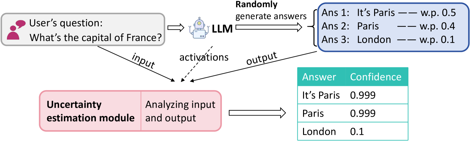</details> Figure 1: An example to illustrate the uncertainty estimation task. The LLM randomly generates an answer to the question (It’s Paris, Paris, or London). The goal of the uncertainty estimation is to estimate a confidence score to the question-answer pair, where a higher score indicates a higher confidence in the correctness of the answer. In this work, we aim to formally define the problem of uncertainty estimation for LLMs and propose methods to address it. As shown in Figure 1, uncertainty estimation for LLMs can be broadly defined as the task of predicting the quality of the generated response based on the input. In this context, “quality” typically refers to aspects such as confidence, truthfulness, and uncertainty. Assuming access to a universal metric for evaluating the confidence of the output, the goal of uncertainty estimation is to produce a confidence score that closely aligns with this metric. Given the inherent randomness in LLMs, where incorrect responses can still be generated with positive probability, uncertainty estimation serves as a crucial safeguard. It helps assess the reliability of responses, enhance the trustworthiness of the model, and guide users on when to trust or question the output. It is also worth noting that calibration is closely related and can be viewed as a subclass of uncertainty estimation, where the metric corresponds to the conditional probability in the individual level. Most studies on uncertainty estimation or calibration in language models focus on fixed-dimensional prediction tasks (i.e., the output of the LLM only has one token limited in a finite set), such as sentiment analysis, natural language inference, and commonsense reasoning (Zhou et al., 2023; Si et al., 2022; Xiao et al., 2022; Desai and Durrett, 2020). However, given the structural differences in how modern LLMs are used, alongside their proven capability to handle complex, free-form tasks with variable-length outputs, there is a growing need to address uncertainty estimation and calibration specifically for general language tasks in the domain of LLMs. This work explores a simple supervised method motivated by two ideas in the existing literature on LLMs. First, prior work on uncertainty estimation for LLMs primarily focused on designing uncertainty metrics in an unsupervised way by examining aspects like the generated outputs’ consistency, similarity, entropy, and other relevant characteristics (Lin et al., 2023; Manakul et al., 2023; Kuhn et al., 2023; Hou et al., 2023; Lin et al., 2022; Kuhn et al., 2023; Chen et al., 2024). The absence of the need for knowledge of the model’s weights enables their application to some black-box or gray-box models. Second, a growing stream of literature argues that hidden layers’ activation values within the LLMs offer insights into the LLMs’ knowledge and confidence (Slobodkin et al., 2023; Ahdritz et al., 2024; Duan et al., 2024). It has shown success in other fields of LLMs, like hallucination detection (CH-Wang et al., 2023; Azaria and Mitchell, 2023; Ahdritz et al., 2024). Based on this argument, white-box LLMs, which allow access to more of LLMs’ internal states, such as logits and hidden layers, are believed to have the capacity to offer a more nuanced understanding and improved uncertainty estimation results (Verma et al., 2023; Chen et al., 2024; Plaut et al., 2024). 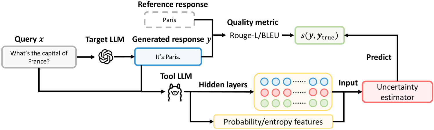Both of the above approaches, however, have key limitations. For the unsupervised metrics, given the complexity of LLMs’ underlying architectures, semantic information may be diluted when processing through self-attention mechanisms and during token encoding/decoding. For the second idea, the requirements of hidden layer features restrict its application to close-source/black-box LLMs. In this paper, we combine the strengths of these two ideas by proposing a general supervised learning method and pipeline design that address these limitations. Specifically, to incorporate more features (e.g., hidden layers) in estimating the uncertainty, we train an external uncertainty estimation model in a supervised way to estimate the uncertainty/confidence of the response generated from an LLM (target LLM). As the quality of the response reveals to what extent we should believe the response is correct, we formulate this supervised uncertainty estimation problem as a regression task and prepare the labels in the training dataset by measuring the response’s quality. To extend our method to black-box LLMs, we allow the semantic features of the question-response pair to come from another language model (tool LLM). The overall pipeline of this method is shown in Figure 2. <details> <summary>x2.png Details</summary>  ### Visual Description ## Flowchart: Response Generation and Quality Evaluation System ### Overview The flowchart illustrates a technical system for generating and evaluating responses to queries using language models (LLMs). It shows the flow from a user query through response generation, quality assessment, and uncertainty estimation. Key components include a target LLM, reference response, quality metric, hidden layers, and an uncertainty estimator. ### Components/Axes 1. **Query (x)**: Input question ("What's the capital of France?") 2. **Target LLM**: Generates response ("It's Paris.") 3. **Reference Response**: Ground truth answer ("Paris") 4. **Quality Metric**: Evaluates response using Rouge-L/BLEU scores 5. **Uncertainty Estimator**: Predicts uncertainty based on hidden layer features 6. **Tool LLM**: Processes hidden layers to extract probability/entropy features 7. **Hidden Layers**: Represented by colored circles (blue, red, green) 8. **Probability/Entropy Features**: Output from hidden layers 9. **Color Coding**: - Blue: Target LLM/Generated response - Red: Uncertainty estimator - Green: Quality metric - Yellow: Hidden layers/Probability/entropy features ### Detailed Analysis - **Query Flow**: - Query `x` → Target LLM → Generated response `y` ("It's Paris.") - Reference response ("Paris") is compared to `y` via quality metric. - **Quality Metric**: - Outputs `s(y, y_true)` (score comparing generated vs. reference response). - **Uncertainty Estimator**: - Takes input from hidden layers (colored circles) to predict uncertainty. - Hidden layers process probability/entropy features (yellow box). - **Color Consistency**: - Blue elements (Target LLM, Generated response) match blue circles in hidden layers. - Red elements (Uncertainty estimator) match red circles. - Green elements (Quality metric) match green circles. ### Key Observations 1. **Linear Workflow**: Query → Response Generation → Quality Evaluation → Uncertainty Estimation. 2. **Feedback Loop**: Reference response and quality metric likely inform improvements to the target LLM. 3. **Uncertainty Source**: Uncertainty is derived from hidden layer activity (probability/entropy), suggesting confidence assessment in the response. 4. **Missing Numerical Data**: No specific scores or values are provided for Rouge-L/BLEU or uncertainty metrics. ### Interpretation This system demonstrates a closed-loop approach to LLM response generation and evaluation. The integration of quality metrics (Rouge-L/BLEU) ensures responses align with reference answers, while the uncertainty estimator uses internal model dynamics (hidden layers) to quantify confidence. The lack of numerical data points suggests the diagram emphasizes architectural relationships over empirical results. The use of probability/entropy features implies a focus on epistemic uncertainty (model knowledge gaps) rather than aleatoric uncertainty (data noise). The color-coded components visually separate distinct stages, aiding in understanding the system's modular design. </details> Figure 2: Illustration of our proposed supervised method. The tool LLM is an open-source LLM and can be different from the target LLM. In the training phase, where the reference response is available, we train the uncertainty estimator using the quality of the response as the label. In the test phase, the uncertainty estimator predicts the quality of the generated response to obtain an uncertainty score. Our contributions are four-fold: - First, we formally define the task of uncertainty estimation, while some of the existing literature either does not distinguish uncertainty estimation and uncertainty calibration or misuses and confuses the terminologies of uncertainty and hallucination. - Second, we adopt a supervised method for uncertainty estimation that is intuitive, easy to implement, and executable even on black-box LLMs. Leveraging supervised labels from the uncertainty metric, our approach sets an upper bound for the performance of all unsupervised methods, representing the highest achievable performance for these approaches. - Third, we systematically discuss the relationship and the difference between deep learning and LLM in uncertainty estimation. Formally, we give an explanation to see why the method for the traditional deep learning model may fail in LLM, and why the hidden layer is useful in estimating the uncertainty in our context. - Finally, numerical experiments on various natural language processing tasks demonstrate the superiority of our methods over existing benchmarks. The results also reveal several insightful observations, including the role of neural nodes in representing uncertainty, and the transferability of our trained uncertainty estimation model. ### 1.1 Related literature The uncertainty estimation and calibration for traditional machine learning is relatively well-studied (Abdar et al., 2021; Gawlikowski et al., 2023). However, with the rapid development of LLMs, there is a pressing need to better understand the uncertainty for LLMs’ responses, and measuring the uncertainty from sentences instead of a fixed-dimension output is more challenging. One stream of work has been focusing on unsupervised methods that leverage entropy (Malinin and Gales, 2021), similarity (Fomicheva et al., 2020; Lin et al., 2022), semantic (Kuhn et al., 2023; Duan et al., 2023), logit or hidden states’ information (Kadavath et al., 2022; Chen et al., 2024; Su et al., 2024; Plaut et al., 2024) to craft an uncertainty metric that helps to quantify uncertainty. For black-box models, some of the metrics can be computed based on multiple sampled output of the LLMs (Malinin and Gales, 2021; Lin et al., 2023; Manakul et al., 2023; Chen and Mueller, 2023); while for white-box models, more information such as the output’s distribution, the value of the logit and hidden layers make computing the uncertainty metric easier. We also refer to Desai and Durrett (2020); Zhang et al. (2021); Ye and Durrett (2021); Si et al. (2022); Quach et al. (2023); Kumar et al. (2023); Mohri and Hashimoto (2024) for other related uncertainty estimation methods such as conformal prediction. We defer more discussions on related literature, in particular, on the topics of hallucination detection and information in hidden layers of LLMs, to Appendix A. ## 2 Problem Setup Consider the following environment where one interacts with LLMs through prompts and responses: An LLM is given with an input prompt $\bm{x}=(x_{1},x_{2},...,x_{k})\in\mathcal{X}$ with $x_{i}\in\mathcal{V}$ representing the $i$ -th token of the prompt. Here $\mathcal{V}$ denotes the vocabulary for all the tokens. Then the LLM randomly generates its response $\bm{y}=(y_{1},y_{2},...,y_{m})\in\mathcal{Y}$ following the probability distribution $$ y_{j}\sim p_{\theta}(\cdot|\bm{x},y_{1},y_{2},...,y_{j-1}). $$ Here the probability distribution $p_{\theta}$ denotes the distribution (over vocabulary $\mathcal{V}$ ) as the LLM’s output, and $\theta$ encapsulates all the parameters of the LLM. The conditional part includes the prompt $\bm{x}$ and all the tokens $y_{1},y_{2},...,y_{j-1}$ generated preceding the current position. We consider using the LLM for some downstream NLP tasks such as question answering, multiple choice, and machine translation. Such a task usually comes with an evaluation/scoring function that evaluates the quality of the generated response $s(\cdot,\cdot):\mathcal{Y}\times\mathcal{Y}\rightarrow[0,1].$ For each pair of $(\bm{x},\bm{y}),$ the evaluation function rates the response $\bm{y}$ with the score $z\coloneqq s(\bm{y},\bm{y}_{\text{true}})$ where $\bm{y}_{\text{true}}$ is the true response for the prompt $\bm{x}$ . The true response $\bm{y}_{\text{true}}$ is usually decided by factual truth, humans, or domain experts, and we can assume it follows a distribution condition on the prompt $\bm{x}$ . It does not hurt to assume a larger score represents a better answer; $z=1$ indicates a perfect answer, while $z=0$ says the response $\bm{y}$ is off the target. We define the task of uncertainty estimation for LLMs as the learning of a function $g$ that predicts the score $$ g(\bm{x},\bm{y})\approx\mathbb{E}\left[s(\bm{y},\bm{y}_{\text{true}})|\bm{x}, \bm{y}\right] \tag{1} $$ where the expectation on the right-hand side is taken with respect to the (possible) randomness of the true response $\bm{y}_{\text{true}}$ , and for notational clarity, we omit the dependence of $\bm{y}_{\text{true}}$ on $\bm{x}$ . We emphasize two points on this task definition: The uncertainty function $g$ takes the prompt $\bm{x}$ and $\bm{y}$ as its inputs. This implies (i) the true and predicted uncertainty score can and should depend on the specific realization of the response $\bm{y}$ , not just $\bm{x}$ (Zhang et al., 2021; Kuhn et al., 2023), and (ii) the uncertainty function $g$ does not require the true response $\bm{y}_{\text{true}}$ as the input. We note that a significant body of literature explores uncertainty estimation and calibration in language models (Zhou et al., 2023; Si et al., 2022; Xiao et al., 2022; Desai and Durrett, 2020). They primarily focus on classification tasks where outputs are limited to a finite set of tokens (i.e., $\bm{y}$ contains only one element). In contrast, our work extends this to allow free-form responses, and the ability to handle variable-length outputs aligns more closely with current advancements in LLMs. ## 3 Uncertainty Estimation via Supervised Learning ### 3.1 Overview of supervised uncertainty estimation We consider a supervised approach of learning the uncertainty function $g:\mathcal{X}\times\mathcal{Y}\rightarrow[0,1]$ , which is similar to the standard setting of uncertainty quantification for ML/deep learning models. First, we start with a raw dataset of $n$ samples $$ \mathcal{D}_{\text{raw}}=\left\{(\bm{x}_{i},\bm{y}_{i},\bm{y}_{i,\text{true}}, s(\bm{y}_{i},\bm{y}_{i,\text{true}}))\right\}_{i=1}^{n}. $$ $\mathcal{D}_{\text{raw}}$ can be generated based on a labeled dataset for the tasks we consider. Here $\bm{x}_{i}=(x_{i,1},...,x_{i,k_{i}})$ and $\bm{y}_{i}=(y_{i,1},...,y_{i,m_{i}})$ denote the prompt and the corresponding LLM’s response, respectively. $\bm{y}_{i,\text{true}}$ denotes the true response (that comes from the labeled dataset) of $\bm{x}_{i}$ , and $s(\bm{y}_{i},\bm{y}_{i,\text{true}})$ assigns a score for the response $\bm{y}_{i}$ based on the true answer $\bm{y}_{i,\text{true}}$ . The next is to formulate a supervised learning task based on $\mathcal{D}_{\text{raw}}$ . Specifically, we construct $$ \mathcal{D}_{\text{sl}}=\left\{(\bm{v}_{i},z_{i})\right\}_{i=1}^{n} $$ where $z_{i}\coloneqq s(\bm{y}_{i},\bm{y}_{i,\text{true}})\in[0,1]$ denotes the target score to be predicted. The vector $\bm{v}_{i}$ summarizes useful features for the $i$ -th sample based on $(\bm{x}_{i},\bm{y}_{i})$ . With this design, a supervised learning task on the dataset $\mathcal{D}_{\text{sl}}$ coincides exactly with learning the uncertainty estimation task defined in (1). Getting Features. When constructing $\bm{v}_{i}$ , a natural implementation is to use the features of $(\bm{x},\bm{y})$ extracted from the LLM (denoted as target LLM) that generates the response $\bm{y}$ as done in Duan et al. (2024) for hallucination detection and Burns et al. (2022) for discovering latent knowledge. This method functions effectively with white-box LLMs where hidden activations are accessible. We note that obtaining hidden layers’ activations merely requires an LLM and the prompt-response pair $(\bm{x},\bm{y})$ , and the extra knowledge of uncertainty can come from the hidden layers of any white-box LLM that takes as input the $(\bm{x},\bm{y})$ pair, not necessarily from the target LLM. Another note is that our goal is to measure the uncertainty of the input-output pair $(\bm{x},\bm{y})$ using the given metric, which is independent of the target LLM that generates the output from input $\bm{x}$ . Therefore, due to the unique structure of LLMs, any white-box LLM can take $(\bm{x},\bm{y})$ together as input, allowing us to extract features from this white-box LLM (referred to as the tool LLM). This observation has two implications: First, if the target LLM is a black-box one, we can rely on a white-box tool LLM to extract feature; Second, even if the target LLM is a Which-box one, we can also adopt a more powerful white-box tool LLM) that could potentially generate more useful feature. In Algorithm 1, we present the algorithm of our pipeline that is applicable to target LLMs of any type, and we provide an illustration of the algorithm pipeline in Figure 2. Algorithm 1 Supervised uncertainty estimation 1: Target LLM $p_{\theta}$ (the uncertainty of which is to be estimated), tool LLM $q_{\theta}$ (used for uncertainty estimation), a labeled training dataset $\mathcal{D}$ , a test sample with prompt $\bm{x}$ 2: %% Training phase: 3: Use $p_{\theta}$ to generate responses for the samples in $\mathcal{D}$ and construct the dataset $\mathcal{D}_{\text{raw}}$ 4: For each sample $(\bm{x}_{i},\bm{y}_{i})\in\mathcal{D}_{\text{raw}}$ , extract features (hidden-layer activations, entropy- and probability-related features) using the LLM $q_{\theta}$ , and then construct the dataset $\mathcal{D}_{\text{sl}}$ 5: Train a supervised learning model $\hat{g}$ that predicts $z_{i}$ with $\bm{v}_{i}$ based on the dataset $\mathcal{D}_{\text{sl}}$ 6: %% Test phase: 7: Generate the response $\bm{y}$ for the test prompt $\bm{x}$ 8: Extract features $\bm{v}$ using $q_{\theta}$ 9: Associate the response $\bm{y}$ with the uncertainty score $\hat{g}(\bm{v})$ ### 3.2 Features for uncertainty estimation A bunch of features that can be extracted from an LLM show a potential relationship to the measurement of uncertainty in the literature. Here we categorize these features into two types based on their sources: White-box features: LLM’s hidden-layer activations. We feed $(\bm{x}_{i},\bm{y}_{i})$ as input into the tool LLM, and extract the corresponding hidden layers’ activations of the LLM. Grey-box features: Entropy- or probability-related outputs. The entropy of a discrete distribution $p$ over the vocabulary $\mathcal{V}$ is defined by $H(p)\coloneqq-\sum_{v\in\mathcal{V}}p(v)\log\left(p(v)\right).$ For a prompt-response pair $(\bm{x},\bm{y})=(x_{1},...,x_{k},y_{1},...,y_{m})$ , we consider as the features the entropy at each token such as $H(q_{\theta}(\cdot|x_{1},...,x_{j-1}))$ and $H(q_{\theta}(\cdot|\bm{x},y_{1},...,y_{j-1}))$ where $q_{\theta}$ denotes the tool LLM. We defer the detailed discussions on feature construction to Appendix D. There can be other useful features such as asking the LLM “how certain it is about the response” (Tian et al., 2023). We do not try to exhaust all the possibilities, and the aim of our paper is more about formulating the uncertainty estimation for the LLMs as a supervised task and understanding how the internal states of the LLM encode uncertainty. To the best of our knowledge, our paper is the first one to do so. Specifically, the above formulation aims for the following two outcomes: (i) an uncertainty model $\hat{g}(\bm{v}_{i})$ that predicts $z_{i}$ and (ii) knowing whether the hidden layers carry the uncertainty information. ### 3.3 Three regimes of supervised uncertainty estimation In Section 3.1, we present that our supervised uncertainty estimation method can be extended to a black-box LLM by separating the target LLM and tool LLM. Next, we formally present our method for white-box, grey-box, and black-box target LLMs. White-box supervised uncertainty estimation (Wb-S): This Wb-S approach is applicable to a white-box LLM where the tool LLM coincides with the target LLM (i.e., $p_{\theta}=q_{\theta}$ ). Grey-box supervised uncertainty estimation (Gb-S): This Gb-S regime also uses the same target and tool LLMs ( $p_{\theta}=q_{\theta}$ ) and constructs the features only from the grey-box source, that is, those features relying on the probability and the entropy (such as those in Table 5 in Appendix D), but it ignores the hidden-layer activations. Black-box supervised uncertainty estimation (Bb-S): The Bb-S regime does not assume the knowledge of the parameters of $p_{\theta}$ but still aims to estimate its uncertainty. To achieve this, it considers another open-source LLM denoted by $q_{\theta}$ . The original data $\mathcal{D}_{\text{raw}}$ is generated by $p_{\theta}$ but then the uncertainty estimation data $\mathcal{D}_{\text{sl}}$ is constructed based on $q_{\theta}$ from $\mathcal{D}_{\text{raw}}$ as illustrated in the following diagram $$ \mathcal{D}_{\text{raw}}\overset{q_{\theta}}{\longrightarrow}\mathcal{D}_{ \text{sl}}. $$ For example, for a prompt $\bm{x}$ , a black-box LLM $p_{\theta}$ generates the response $\bm{y}.$ We utilize the open-source LLM $q_{\theta}$ to treat $(\bm{x},\bm{y})$ jointly as a sequence of (prompt) tokens and extract the features of hidden activations and entropy as in Section 3.2. In this way, we use $q_{\theta}$ together with the learned uncertainty model from $\mathcal{D}_{\text{sl}}$ to estimate the uncertainty of responses generated from $p_{\theta}$ which we do not have any knowledge about. ## 4 Insights for the algorithm design ### 4.1 Uncertainty estimation v.s. uncertainty calibration So far in this paper, we focus on the uncertainty estimation task which aims to predict the quality of the response to reveal whether the LLM makes mistakes in its response or not. There is a different but related task known as the uncertainty calibration problem. In comparison, the uncertainty calibration aims to ensure that the output from the uncertainty estimation model for (1) conveys a probabilistic meaning. That is, $g(\bm{x},\bm{y})$ is defined as the probability that $\bm{y}$ is true. This is compatible with our method by replacing the quality $s(\bm{y},\bm{y}_{\text{true}})$ with $1\left\{\bm{y}\in\mathcal{Y}_{\text{true}}\right\}$ , where $\mathcal{Y}_{\text{true}}$ is a set containing all the possible true responses. Another aspect of the relation between our uncertainty estimation method and uncertainty calibration is that our method can be followed by any recalibration methods for ML models to form a pipeline for calibration. And intuitively, a better uncertainty estimation/prediction will lead to a better-calibrated uncertainty model, which is also verified in our numerical experiments in Appendix C. ### 4.2 Why hidden layers as features? In this subsection, we provide a simple theoretical explanation for why the hidden activations of the LLM can be useful in uncertainty estimation. Consider a binary classification task where the features $\bm{X}\in\mathbb{R}^{d}$ and the label $Y\in\{0,1\}$ are drawn from a distribution $\mathcal{P}.$ We aim to learn a model $f:\mathbb{R}^{d}\rightarrow[0,1]$ that predicts the label $Y$ from the feature vector $\bm{X}$ , and the learning of the model employs a loss function $l(\cdot,\cdot):[0,1]\times[0,1]\rightarrow\mathbb{R}$ . **Proposition 4.1** *Let $\mathcal{F}$ be the class of measurable function that maps from $\mathbb{R}^{d}$ to $[0,1]$ . Under the cross-entropy loss $l(y,\hat{y})=y\log(\hat{y})+(1-y)\log(1-\hat{y})$ , the function $f^{*}$ that minimizes the loss $$ f^{*}=\operatorname*{arg\,min}_{f\in\mathcal{F}}\mathbb{E}\left[l(Y,f(\bm{X}))\right] $$ is the Bayes optimal classifier $f^{*}(\bm{x})=\mathbb{P}(Y=1|\bm{X}=\bm{x})$ where the expectation and the probability are taken with respect to $(\bm{X},Y)\sim\mathcal{P}.$ Moreover, the following conditional independence holds $$ Y\perp\bm{X}\ |\ f^{*}(\bm{X}). $$* The proposition is not technical and it can be easily proved by using the structure of $f^{*}(\bm{X})$ so we refer the proof to Berger (2013). It states a nice property of the cross-entropy loss that the function learned under the cross-entropy loss coincides with the Bayes optimal classifier. Note that this is contingent on two requirements. First, the function class $\mathcal{F}$ is the measurable function class. Second, it requires the function $f^{*}$ learned through the population loss rather than the empirical loss/risk. The proposition also states one step further on conditional independence $Y\perp\bm{X}\ |\ f^{*}(\bm{X})$ . This means all the information related to the label $Y$ that is contained in $\bm{X}$ is summarized in the prediction function $f^{*}.$ This intuition suggests that for classic uncertainty estimation problems, when a prediction model $\hat{f}:\mathbb{R}^{d}\rightarrow[0,1]$ is well-trained, the predicted score $\hat{f}(\bm{X})$ should capture all the information about the true label $Y$ contained in the features $\bm{X}$ , without relying on the features of $\bm{X}$ . This indeed explains why the classic uncertainty estimation and calibration methods only work with the predicted score $\hat{f}(\bm{X})$ for re-calibration, including Platt scaling (Platt et al., 1999), isotonic regression (Zadrozny and Elkan, 2002), temperature scaling (Guo et al., 2017), etc. When it comes to uncertainty estimation for LLMs, which is different from calibration and LLMs’ structure is much more complex, we will no longer have conditional independence, and that requires additional procedures to retrieve more information on $Y$ . The following supporting corollary states that when the underlying loss function $\tilde{l}$ does not possess this nice property (the Bayes classifier minimizes the loss point-wise) of the cross-entropy loss, the conditional independence will collapse. **Corollary 4.2** *Suppose the loss function $\tilde{l}$ satisfies $$ \mathbb{P}\left(f^{*}(\bm{x})\neq\operatorname*{arg\,min}_{\tilde{y}\in[0,1]} \mathbb{E}\left[\tilde{l}(Y,\tilde{y})|\bm{X}=\bm{x}\right]\right)>0, $$ where $f^{*}$ is defined as Proposition 4.1, then for the function $\tilde{f}=\operatorname*{arg\,min}_{f\in\mathcal{F}}\mathbb{E}\left[\tilde{l}( Y,f(\bm{X}))\right],$ where the expectation is with respect to $(\bm{X},Y)\sim\mathcal{P},$ there exists a distribution $\mathcal{P}$ such that the conditional independence no longer holds $$ Y\not\perp\bm{X}\ |\ \tilde{f}(\bm{X}). $$* Proposition 4.1 and Corollary 4.2 together illustrate the difference between uncertainty estimation for a traditional ML model and that for LLMs. In this task, the output $\tilde{f}(\bm{X})$ of the model (traditional ML model or LLM) is restricted in [0,1] to indicate the confidence of $Y=1$ . For the traditional ML models, the cross-entropy loss, which is commonly used for training the model, is aligned toward the uncertainty calibration objective. When it comes to uncertainty estimation for LLMs, the objective can be different from calibration, and the LLMs are often pretrained with some other loss functions (for example, the negative log-likelihood loss for next-token prediction) on diverse language tasks besides binary classifications. These factors cause a misalignment between the model pre-training and the uncertainty estimation task. Consequently, the original features (e.g., the output logits) may and should (in theory) contain information about the uncertainty score $Y$ that cannot be fully captured by $\tilde{f}(\bm{X})$ . This justifies why we formulate the uncertainty estimation task as the previous subsection and take the hidden-layer activations as features to predict the uncertainty score; it also explains why we do not see much similar treatment in the mainstream uncertainty estimation literature (Kuhn et al., 2023; Manakul et al., 2023; Tian et al., 2023). ## 5 Numerial Experiments and Findings In this section, we provide a systematic evaluation of the proposed supervised approach for estimating the uncertainty of the LLMs. All code used in our experiments is available at https://github.com/LoveCatc/supervised-llm-uncertainty-estimation. ### 5.1 LLMs, tasks, benchmarks, and performance metrics Here we outline the general setup of the numerical experiments. Certain tasks may deviate from the general setup, and we will detail the specific adjustments as needed. LLMs. For our numerical experiments, we mainly consider three open-source LLMs, LLaMA2-7B (Touvron et al., 2023), LLaMA3-8B (AI@Meta, 2024) and Gemma-7B (Gemma Team et al., 2024) as $p_{\theta}$ defined in Section 2. For certain experiments, we also employ the models of LLaMA2-13B and Gemma-2B. We also use their respective tokenizers as provided by Hugging Face. We do not change the parameters/weights $\theta$ of these LLMs. Tasks and Datasets. We mainly consider three tasks for uncertainty estimation, question answering, multiple choice, and machine translation. All the labeled datasets for these tasks are in the form of $\{(\bm{x}_{i},\bm{y}_{i,\text{true}})\}_{i=1}^{n}$ where $\bm{x}_{i}$ can be viewed as the prompt for the $i$ -th sample and $\bm{y}_{i,\text{true}}$ the true response. We adopt the few-shot prompting when generating the LLM’s response $\bm{y}_{i}$ , and we use 5 examples in the prompt of the multiple-choice task and 3 examples for the remaining natural language generation tasks. This enables the LLM’s in-context learning ability (Radford et al., 2019; Zhang et al., 2023) and ensures the LLM’s responses are in a desirable format. We defer more details of the few-shot prompting to Appendix D.1. The three tasks are: - Question answering. We follow Kuhn et al. (2023) and use the CoQA and TriviaQA (Joshi et al., 2017) datasets. The CoQA task requires the LLM to answer questions by understanding the provided text, and the TriviaQA requires the LLM to answer questions based on its pre-training knowledge. We adopt the scoring function $s(\cdot,\cdot)$ as Rouge-1 (Lin and Och, 2004a) and label a response $\bm{y}_{i}$ as correct if $s(\bm{y}_{i},\bm{y}_{i,\text{true}})\geq 0.3$ and incorrect otherwise. - Multiple choice. We consider the Massive Multitask Language Understanding (MMLU) dataset (Hendrycks et al., 2020), a collection of 15,858 questions covering 57 subjects across STEM. Due to the special structure of the dataset, the generated output $\bm{y}_{i}$ and the correct answer $\bm{y}_{\text{true},i}\in\{\text{A, B, C, D}\}$ . Therefore, this task can also be regarded as a classification problem for the LLM by answering the question with one of the four candidate choices. - Machine translation. We consider the WMT 2014 dataset (Bojar et al., 2014) for estimating LLM’s uncertainty on the machine translation task. The scoring function $s(\cdot,\cdot)$ is chosen to be the BLEU score (Papineni et al., 2002; Lin and Och, 2004b) and the generated answer $\bm{y}_{i}$ is labeled as correct if $s(\bm{y}_{i},\bm{y}_{i,\text{true}})>0.3$ and incorrect otherwise. Benchmarks. We compare our approach with a number of the state-of-the-art benchmarks for the problem. Manakul et al. (2023) give a comprehensive survey of the existing methods and compare four distinct measures for predicting sentence generation uncertainty. The measures are based on either the maximum or average values of entropy or probability across the sentence, including Max Likelihood, Avg Likelihood, Max Ent, and Avg Ent defined in Table 5. We note that each of these measures can be applied as a single uncertainty estimator, and they are all applied in an unsupervised manner that does not require additional supervised training. In particular, in applying these measures for the MMLU dataset, since the answer only contains one token from $\{\text{A, B, C, D}\}$ , we use the probabilities and the entropy (over these four tokens) as the benchmarks which represent the probability of the most likely choice and the entropy of all choices, respectively. Kuhn et al. (2023) generate multiple answers, compute their entropy in a semantic sense, and define the quantity as semantic entropy. This semantic-entropy uncertainty (SU) thus can be used as an uncertainty estimator for the LLM’s responses. Tian et al. (2023) propose the approach of asking the LLM for its confidence (denoted as A4U) which directly obtains the uncertainty score from the LLM itself. Our methods. We follow the discussions in Section 3.3 and implement three versions of our proposed supervised approach: black-box supervised (Bb-S), grey-box supervised (Gb-S), and white-box supervised (Wb-S). These models have the same pipeline of training the uncertainty estimation model and the difference is only on the availability of the LLM. For the Bb-S method, we use the Gemma-7B as the model $q_{\theta}$ to evaluate the uncertainty of LLaMA2-7B/LLaMA3-8B $p_{\theta}$ (treated as a black-box), and reversely, use LLaMA2-7B to evaluate Gemma-7B. The supervised uncertainty model $\hat{g}$ is trained based on the random forest model (Breiman, 2001). Details on the feature construction and the training of the random forest model are deferred to Appendix D.2. Performance metrics. For the model evaluation, we follow Filos et al. (2019); Kuhn et al. (2023) and compare the performance of our methods against the benchmark using the generated uncertainty score to predict whether the answer is correct. The area under the receiver operator characteristic curve (AUROC) metric is employed to measure the performance of the uncertainty estimation. As discussed in Section 4.1, AUROC works as a good metric for the uncertainty estimation task whereas for the uncertainty calibration task, we follow the more standard calibration metrics and present the results in Section C. ### 5.2 Performance of uncertainty estimation Now we present the performance on the uncertainty estimation task. #### 5.2.1 Question answering and machine translation The question answering and machine translation tasks can all be viewed as natural language generation tasks so we present their results together. Table 1 summarizes the three versions of our proposed supervised method against the existing benchmarks in terms of AUROC. | TriviaQA | G-7B | 0.857 | 0.862 | 0.849 | 0.854 | 0.847 | 0.534 | 0.879 | 0.866 | 0.882 | | --- | --- | --- | --- | --- | --- | --- | --- | --- | --- | --- | | L-7B | 0.565 | 0.761 | 0.761 | 0.773 | 0.678 | 0.526 | 0.925 | 0.811 | 0.897 | | | L-8B | 0.838 | 0.851 | 0.849 | 0.853 | 0.826 | 0.571 | 0.843 | 0.861 | 0.874 | | | CoQA | G-7B | 0.710 | 0.708 | 0.725 | 0.708 | 0.674 | 0.515 | 0.737 | 0.737 | 0.762 | | L-7B | 0.535 | 0.600 | 0.603 | 0.580 | 0.541 | 0.502 | 0.848 | 0.667 | 0.807 | | | L-8B | 0.692 | 0.697 | 0.716 | 0.699 | 0.684 | 0.506 | 0.745 | 0.737 | 0.769 | | | WMT-14 | G-7B | 0.668 | 0.589 | 0.637 | 0.811 | 0.572 | 0.596 | 0.863 | 0.829 | 0.855 | | L-7B | 0.606 | 0.712 | 0.583 | 0.711 | 0.513 | 0.506 | 0.792 | 0.724 | 0.779 | | | L-8B | 0.554 | 0.685 | 0.616 | 0.729 | 0.510 | 0.502 | 0.700 | 0.724 | 0.745 | | Table 1: Out-of-sample AUROC performance for benchmarks and our methods on natural language generation tasks. G-7B, L-7B, and L-8B represent Gemma-7B, LLaMA2-7B, and LLaMA-8B, respectively. The columns MaxL, AvgL, MaxE, and AvgE all come from Manakul et al. (2023). The column SU implements the semantic uncertainty estimation by Kuhn et al. (2023), and the column A4C implements the ask-for-confidence method by Tian et al. (2023). The columns Bb-S, Gb-S, and Wb-S represent respectively the three regimes (black-box supervised, grey-box supervised, and white-box supervised) of our supervised method with details in Section 3.3. We make several remarks on the numerical results. First, our methods generally have a better performance than the existing benchmarks. Note that the existing benchmarks are mainly unsupervised and based on one single score, and also that our method proceeds with the most standard pipeline for supervised training of an uncertainty estimation model. The advantage of our method should be attributed to the supervised nature and the labeled dataset. While these unsupervised benchmark methods can work in a larger scope than these NLP tasks (though they have not been extensively tested on open questions yet), our methods rely on the labeled dataset. But in addition to these better numbers, the experiment results show the potential of labeled datasets for understanding the uncertainty in LLM’s responses. In particular, our method Gb-S uses features including the benchmark methods, and it shows that some minor supervised training can improve a lot upon the ad-hoc uncertainty estimation based on one single score such as MaxL or MaxE. Second, our method Wb-S has a clear advantage over our method Gb-S. Note that these two methods differ in that the Wb-S uses the hidden activations while the Gb-S only uses probability-related (and entropy-related) features. This implies that the hidden activations do contain uncertainty information which we will investigate more in Appendix B. Also, we note from the table that there is no single unsupervised grey-box method (under the Benchmarks columns) that consistently surpasses others across different datasets/NLP tasks. For example, among all these unsupervised benchmark methods for grey-box LLMs, AvgE emerges as a top-performing one for the Gemma-7B model when applied to the machine translation task, but it shows the poorest performance for the same Gemma-7B model when tested on the question-answering CoQA dataset. This inconsistency highlights some caveats when using the unsupervised approach for uncertainty estimation of LLMs. Lastly, we note that the Bb-S method has a similar or even better performance as the Wb-S method. As discussed in Section 3.3, the performance of uncertainty estimation relies on the LLM that we use to evaluate the prompt-response pair. Therefore, it is not surprising to see that in the question-answering task, for answers generated by LLaMA2-7B, Bb-S features better uncertainty estimation than Wb-S, possibly because Gemma-7B, the LLM that is used as the “tool LLM” in Algorithm 1, encodes better knowledge about the uncertainty of the answers than LLaMA-7B. We also note that the performance of Bb-S is not always as good as Wb-S, and we hypothesize that it is because LLMs’ output distribution differs, which could result in evaluating the uncertainty of different answers. Despite these inconsistencies, the performance of Bb-S is still strong, and these results point to a potential future avenue for estimating the uncertainty of closed-source LLMs. #### 5.2.2 Multiple choice (MMLU) Table 2 presents the performance of our methods against the benchmark methods on the MMLU dataset. For this multiple choice task, the output is from {A,B,C,D} which bears no semantic meaning, and therefore we do not include the Semantic Uncertainty (SU) as Table 1. The results show the advantage of our proposed supervised approach, consistent with the previous findings in Table 1. | Gemma-7B LLaMA2-7B LLaMA3-8B | 0.712 0.698 0.781 | 0.742 0.693 0.791 | 0.582 0.514 0.516 | 0.765 0.732 0.766 | 0.776 0.698 0.793 | 0.833 0.719 0.830 | | --- | --- | --- | --- | --- | --- | --- | Table 2: Out-of-sample AUROC performance for benchmarks and our methods on the MMLU dataset. The columns Probability and Entropy come from Manakul et al. (2023), and the column A4C implements the ask-for-confidence method by Tian et al. (2023). The columns Bb-S, Gb-S, and Wb-S represent respectively the three regimes (black-box supervised, grey-box supervised, and white-box supervised) of our supervised method with details in Section 3.3. We defer more numerical experiments and visualization to Appendices B and C where we investigate more on (i) the effect of the choice of layers; (ii) the scale of the LLMs used; (iii) the uncertainty neurons of the LLMs; and (iv) the calibration performance. ### 5.3 Transferability In this subsection, we evaluate the robustness of our methods under the OOD setting. Setup for the OOD multiple-choice task. We split the MMLU datasets into two groups based on the subjects: Group 1 contains questions from the first 40 subjects while Group 2 contains the remaining 17 subjects, such that the test dataset size of each group is similar (around 600 questions). Note that these 57 subjects span a diverse range of topics, and this means the training and test set can be very different. To test the OOD robustness, we train the proposed methods on one group and evaluate the performance on the other group. Setup for the OOD question-answering task. For the QA task, since we have two datasets (CoQA and TriviaQA), we train the supervised model on either the TriviaQA or CoQA dataset and then evaluate its performance on the other dataset. While both datasets are for question-answering purposes, they diverge notably in two key aspects: (i) CoQA prioritizes assessing the LLM’s comprehension through the discernment of correct responses within extensive contextual passages, while TriviaQA focuses on evaluating the model’s recall of factual knowledge. (ii) TriviaQA typically contains answers comprising single words or short phrases, while CoQA includes responses of varying lengths, ranging from shorter to more extensive answers. | LLMs | Test data | Ours | Best of benchmarks | | | | | --- | --- | --- | --- | --- | --- | --- | | Bb-S | Gb-S | Wb-S | Best GB | Best BB | | | | Transferability in MMLU | | | | | | | | G-7B | Group 1 | 0.756(0.768) | 0.793(0.799) | 0.846(0.854) | 0.765 | 0.538 | | Group 2 | 0.738(0.760) | 0.755(0.754) | 0.804(0.807) | 0.721 | 0.616 | | | L-7B | Group 1 | 0.733(0.749) | 0.715(0.713) | 0.726(0.751) | 0.719 | 0.504 | | Group 2 | 0.700(0.714) | 0.676(0.677) | 0.685(0.692) | 0.679 | 0.529 | | | L-8B | Group 1 | 0.763(0.773) | 0.796(0.795) | 0.836(0.839) | 0.799 | 0.524 | | Group 2 | 0.729(0.761) | 0.786(0.785) | 0.794(0.818) | 0.782 | 0.507 | | | Transferability in Question-Answering Datasets | | | | | | | | G-7B | TriviaQA | 0.842(0.879) | 0.861(0.866) | 0.861(0.882) | 0.862 | 0.847 | | CoQA | 0.702(0.737) | 0.722(0.737) | 0.730(0.762) | 0.725 | 0.674 | | | L-7B | TriviaQA | 0.917(0.925) | 0.801(0.811) | 0.881(0.897) | 0.773 | 0.678 | | CoQA | 0.825(0.848) | 0.623(0.667) | 0.764(0.807) | 0.603 | 0.541 | | | L-8B | TriviaQA | 0.813(0.843) | 0.859(0.861) | 0.863(0.874) | 0.853 | 0.826 | | CoQA | 0.710(0.745) | 0.714(0.737) | 0.725(0.769) | 0.716 | 0.684 | | Table 3: Transferability of the trained uncertainty estimation model across different groups of subjects in MMLU and question-answering datasets. For our proposed Bb-S, Gb-S, and Wb-S methods, values within the parentheses $(\cdot)$ represent the AUROCs where the uncertainty estimation model is trained and tested on the same group of subjects or dataset, while values outside the parentheses represent models trained on another group of subjects or dataset. The Best GB and Best BB columns refer to the best AUROC achieved by the unsupervised grey-box baselines and black-box baselines (fully listed in Table 1 and Table 2), respectively. Table 3 summarizes the performance of these OOD experiments. As expected, for all the methods, there is a slight drop in terms of performance compared to the in-distribution setting (reported by the numbers in the parentheses in the table). We make the following observations based on the experiment results. First, based on the performance gap between in-distribution and OOD evaluation, it is evident that although incorporating white-box features such as hidden activations makes the model more susceptible to performance decreases on OOD tasks, these features also enhance the uncertainty estimation model’s overall capacity, and the benefits outweigh the drawbacks. It is also noteworthy that even in these scenarios of OOD, our Wb-S and Bb-S method almost consistently outperform corresponding baseline approaches. Overall, the robustness of our methods shows that the hidden layers’ activations within the LLM exhibit similar patterns in encoding uncertainty information to some extent. The performance drop (from in-distribution to OOD) observed in the MMLU dataset is notably less than that in the question-answering dataset, which may stem from the larger disparity between the CoQA and TriviaQA datasets compared to that between two distinct groups of subjects within the same MMLU dataset. This suggests that in cases of significant distributional shifts, re-training or re-calibrating the uncertainty estimation model using test data may be helpful. ## 6 Conclusions In this paper, we study the problem of uncertainty estimation and calibration for LLMs. We follow a simple and standard supervised idea and use the labeled NLP datasets to train an uncertainty estimation model for LLMs. Our finding is that, first, the proposed supervised methods have better performances than the existing unsupervised methods. Second, the hidden activations of the LLMs contain uncertainty information about the LLMs’ responses. Third, the black-box regime of our approach (Bb-S) provides a new approach to estimating the uncertainty of closed-source LLMs. Lastly, we distinguish the task of uncertainty estimation from uncertainty calibration and show that a better uncertainty estimation model leads to better calibration performance. One limitation of our proposed supervised method is that it critically relies on the labeled data. For the scope of our paper, we restrict the discussion to the NLP tasks and datasets. One future direction is to utilize the human-annotated data for LLMs’ responses to train a supervised uncertainty estimation model for open-question prompts. We believe the findings that the supervised method gives a better performance and the hidden activations contain the uncertainty information will persist. ## References - Abdar et al. (2021) Abdar, Moloud, Farhad Pourpanah, Sadiq Hussain, Dana Rezazadegan, Li Liu, Mohammad Ghavamzadeh, Paul Fieguth, Xiaochun Cao, Abbas Khosravi, U Rajendra Acharya, et al. 2021. A review of uncertainty quantification in deep learning: Techniques, applications and challenges. Information fusion 76 243–297. - Ahdritz et al. (2024) Ahdritz, Gustaf, Tian Qin, Nikhil Vyas, Boaz Barak, Benjamin L Edelman. 2024. Distinguishing the knowable from the unknowable with language models. arXiv preprint arXiv:2402.03563 . - AI@Meta (2024) AI@Meta. 2024. Llama 3 model card URL https://github.com/meta-llama/llama3/blob/main/MODEL_CARD.md. - Azaria and Mitchell (2023) Azaria, Amos, Tom Mitchell. 2023. The internal state of an llm knows when its lying. arXiv preprint arXiv:2304.13734 . - Berger (2013) Berger, J.O. 2013. Statistical Decision Theory and Bayesian Analysis. Springer Series in Statistics, Springer New York. URL https://books.google.nl/books?id=1CDaBwAAQBAJ. - Bojar et al. (2014) Bojar, Ondřej, Christian Buck, Christian Federmann, Barry Haddow, Philipp Koehn, Johannes Leveling, Christof Monz, Pavel Pecina, Matt Post, Herve Saint-Amand, et al. 2014. Findings of the 2014 workshop on statistical machine translation. Proceedings of the ninth workshop on statistical machine translation. 12–58. - Breiman (2001) Breiman, Leo. 2001. Random forests. Machine learning 45 5–32. - Brown et al. (2020) Brown, Tom, Benjamin Mann, Nick Ryder, Melanie Subbiah, Jared D Kaplan, Prafulla Dhariwal, Arvind Neelakantan, Pranav Shyam, Girish Sastry, Amanda Askell, et al. 2020. Language models are few-shot learners. Advances in neural information processing systems 33 1877–1901. - Bubeck et al. (2023) Bubeck, Sébastien, Varun Chandrasekaran, Ronen Eldan, Johannes Gehrke, Eric Horvitz, Ece Kamar, Peter Lee, Yin Tat Lee, Yuanzhi Li, Scott Lundberg, et al. 2023. Sparks of artificial general intelligence: Early experiments with gpt-4. arXiv preprint arXiv:2303.12712 . - Burns et al. (2022) Burns, Collin, Haotian Ye, Dan Klein, Jacob Steinhardt. 2022. Discovering latent knowledge in language models without supervision. arXiv preprint arXiv:2212.03827 . - Burrell (2016) Burrell, J. 2016. How the machine ‘thinks’: Understanding opacity in machine learning algorithms. Big Data & Society . - CH-Wang et al. (2023) CH-Wang, Sky, Benjamin Van Durme, Jason Eisner, Chris Kedzie. 2023. Do androids know they’re only dreaming of electric sheep? arXiv preprint arXiv:2312.17249 . - Chen et al. (2024) Chen, Chao, Kai Liu, Ze Chen, Yi Gu, Yue Wu, Mingyuan Tao, Zhihang Fu, Jieping Ye. 2024. Inside: Llms’ internal states retain the power of hallucination detection. arXiv preprint arXiv:2402.03744 . - Chen and Mueller (2023) Chen, Jiuhai, Jonas Mueller. 2023. Quantifying uncertainty in answers from any language model and enhancing their trustworthiness . - Desai and Durrett (2020) Desai, Shrey, Greg Durrett. 2020. Calibration of pre-trained transformers. arXiv preprint arXiv:2003.07892 . - Duan et al. (2024) Duan, Hanyu, Yi Yang, Kar Yan Tam. 2024. Do llms know about hallucination? an empirical investigation of llm’s hidden states. arXiv preprint arXiv:2402.09733 . - Duan et al. (2023) Duan, Jinhao, Hao Cheng, Shiqi Wang, Chenan Wang, Alex Zavalny, Renjing Xu, Bhavya Kailkhura, Kaidi Xu. 2023. Shifting attention to relevance: Towards the uncertainty estimation of large language models. arXiv preprint arXiv:2307.01379 . - Esteva et al. (2017) Esteva, Andre, Brett Kuprel, Roberto A Novoa, Justin Ko, Susan M Swetter, Helen M Blau, Sebastian Thrun. 2017. Dermatologist-level classification of skin cancer with deep neural networks. nature 542 (7639) 115–118. - Filos et al. (2019) Filos, Angelos, Sebastian Farquhar, Aidan N Gomez, Tim GJ Rudner, Zachary Kenton, Lewis Smith, Milad Alizadeh, Arnoud de Kroon, Yarin Gal. 2019. Benchmarking bayesian deep learning with diabetic retinopathy diagnosis. Preprint at https://arxiv. org/abs/1912.10481 . - Fomicheva et al. (2020) Fomicheva, Marina, Shuo Sun, Lisa Yankovskaya, Frédéric Blain, Francisco Guzmán, Mark Fishel, Nikolaos Aletras, Vishrav Chaudhary, Lucia Specia. 2020. Unsupervised quality estimation for neural machine translation. Transactions of the Association for Computational Linguistics 8 539–555. - Gal and Ghahramani (2016) Gal, Yarin, Zoubin Ghahramani. 2016. Dropout as a bayesian approximation: Representing model uncertainty in deep learning. international conference on machine learning. PMLR, 1050–1059. - Gawlikowski et al. (2023) Gawlikowski, Jakob, Cedrique Rovile Njieutcheu Tassi, Mohsin Ali, Jongseok Lee, Matthias Humt, Jianxiang Feng, Anna Kruspe, Rudolph Triebel, Peter Jung, Ribana Roscher, et al. 2023. A survey of uncertainty in deep neural networks. Artificial Intelligence Review 56 (Suppl 1) 1513–1589. - Gemma Team et al. (2024) Gemma Team, Thomas Mesnard, Cassidy Hardin, Robert Dadashi, Surya Bhupatiraju, Laurent Sifre, Morgane Rivière, Mihir Sanjay Kale, Juliette Love, Pouya Tafti, Léonard Hussenot, et al. 2024. Gemma doi: 10.34740/KAGGLE/M/3301. URL https://www.kaggle.com/m/3301. - Guo et al. (2017) Guo, Chuan, Geoff Pleiss, Yu Sun, Kilian Q Weinberger. 2017. On calibration of modern neural networks. International conference on machine learning. PMLR, 1321–1330. - Hendrycks et al. (2020) Hendrycks, Dan, Collin Burns, Steven Basart, Andy Zou, Mantas Mazeika, Dawn Song, Jacob Steinhardt. 2020. Measuring massive multitask language understanding. arXiv preprint arXiv:2009.03300 . - Hou et al. (2023) Hou, Bairu, Yujian Liu, Kaizhi Qian, Jacob Andreas, Shiyu Chang, Yang Zhang. 2023. Decomposing uncertainty for large language models through input clarification ensembling. arXiv preprint arXiv:2311.08718 . - Joshi et al. (2017) Joshi, Mandar, Eunsol Choi, Daniel S Weld, Luke Zettlemoyer. 2017. Triviaqa: A large scale distantly supervised challenge dataset for reading comprehension. arXiv preprint arXiv:1705.03551 . - Kadavath et al. (2022) Kadavath, Saurav, Tom Conerly, Amanda Askell, Tom Henighan, Dawn Drain, Ethan Perez, Nicholas Schiefer, Zac Hatfield-Dodds, Nova DasSarma, Eli Tran-Johnson, et al. 2022. Language models (mostly) know what they know. arXiv preprint arXiv:2207.05221 . - Kuhn et al. (2023) Kuhn, Lorenz, Yarin Gal, Sebastian Farquhar. 2023. Semantic uncertainty: Linguistic invariances for uncertainty estimation in natural language generation. arXiv preprint arXiv:2302.09664 . - Kumar et al. (2023) Kumar, Bhawesh, Charlie Lu, Gauri Gupta, Anil Palepu, David Bellamy, Ramesh Raskar, Andrew Beam. 2023. Conformal prediction with large language models for multi-choice question answering. arXiv preprint arXiv:2305.18404 . - Lakshminarayanan et al. (2017) Lakshminarayanan, Balaji, Alexander Pritzel, Charles Blundell. 2017. Simple and scalable predictive uncertainty estimation using deep ensembles. Advances in neural information processing systems 30. - Li et al. (2024) Li, Kenneth, Oam Patel, Fernanda Viégas, Hanspeter Pfister, Martin Wattenberg. 2024. Inference-time intervention: Eliciting truthful answers from a language model. Advances in Neural Information Processing Systems 36. - Lin and Och (2004a) Lin, Chin-Yew, Franz Josef Och. 2004a. Automatic evaluation of machine translation quality using longest common subsequence and skip-bigram statistics. Proceedings of the 42nd annual meeting of the association for computational linguistics (ACL-04). 605–612. - Lin and Och (2004b) Lin, Chin-Yew, Franz Josef Och. 2004b. ORANGE: a method for evaluating automatic evaluation metrics for machine translation. COLING 2004: Proceedings of the 20th International Conference on Computational Linguistics. COLING, Geneva, Switzerland, 501–507. URL https://www.aclweb.org/anthology/C04-1072. - Lin et al. (2023) Lin, Zhen, Shubhendu Trivedi, Jimeng Sun. 2023. Generating with confidence: Uncertainty quantification for black-box large language models. arXiv preprint arXiv:2305.19187 . - Lin et al. (2022) Lin, Zi, Jeremiah Zhe Liu, Jingbo Shang. 2022. Towards collaborative neural-symbolic graph semantic parsing via uncertainty. Findings of the Association for Computational Linguistics: ACL 2022 . - Liu et al. (2023) Liu, Kevin, Stephen Casper, Dylan Hadfield-Menell, Jacob Andreas. 2023. Cognitive dissonance: Why do language model outputs disagree with internal representations of truthfulness? arXiv preprint arXiv:2312.03729 . - Malinin and Gales (2021) Malinin, Andrey, Mark Gales. 2021. Uncertainty estimation in autoregressive structured prediction. International Conference on Learning Representations. URL https://openreview.net/forum?id=jN5y-zb5Q7m. - Manakul et al. (2023) Manakul, Potsawee, Adian Liusie, Mark JF Gales. 2023. Selfcheckgpt: Zero-resource black-box hallucination detection for generative large language models. arXiv preprint arXiv:2303.08896 . - Mielke et al. (2022) Mielke, Sabrina J, Arthur Szlam, Emily Dinan, Y-Lan Boureau. 2022. Reducing conversational agents’ overconfidence through linguistic calibration. Transactions of the Association for Computational Linguistics 10 857–872. - Minderer et al. (2021) Minderer, Matthias, Josip Djolonga, Rob Romijnders, Frances Hubis, Xiaohua Zhai, Neil Houlsby, Dustin Tran, Mario Lucic. 2021. Revisiting the calibration of modern neural networks. Advances in Neural Information Processing Systems 34 15682–15694. - Mohri and Hashimoto (2024) Mohri, Christopher, Tatsunori Hashimoto. 2024. Language models with conformal factuality guarantees. arXiv preprint arXiv:2402.10978 . - Ouyang et al. (2022) Ouyang, Long, Jeffrey Wu, Xu Jiang, Diogo Almeida, Carroll Wainwright, Pamela Mishkin, Chong Zhang, Sandhini Agarwal, Katarina Slama, Alex Ray, et al. 2022. Training language models to follow instructions with human feedback. Advances in neural information processing systems 35 27730–27744. - Papineni et al. (2002) Papineni, Kishore, Salim Roukos, Todd Ward, Wei jing Zhu. 2002. Bleu: a method for automatic evaluation of machine translation. 311–318. - Pedregosa et al. (2011) Pedregosa, Fabian, Gaël Varoquaux, Alexandre Gramfort, Vincent Michel, Bertrand Thirion, Olivier Grisel, Mathieu Blondel, Peter Prettenhofer, Ron Weiss, Vincent Dubourg, et al. 2011. Scikit-learn: Machine learning in python. the Journal of machine Learning research 12 2825–2830. - Platt et al. (1999) Platt, John, et al. 1999. Probabilistic outputs for support vector machines and comparisons to regularized likelihood methods. Advances in large margin classifiers 10 (3) 61–74. - Plaut et al. (2024) Plaut, Benjamin, Khanh Nguyen, Tu Trinh. 2024. Softmax probabilities (mostly) predict large language model correctness on multiple-choice q&a. arXiv preprint arXiv:2402.13213 . - Quach et al. (2023) Quach, Victor, Adam Fisch, Tal Schuster, Adam Yala, Jae Ho Sohn, Tommi S Jaakkola, Regina Barzilay. 2023. Conformal language modeling. arXiv preprint arXiv:2306.10193 . - Radford et al. (2019) Radford, Alec, Jeffrey Wu, Rewon Child, David Luan, Dario Amodei, Ilya Sutskever, et al. 2019. Language models are unsupervised multitask learners. OpenAI blog 1 (8) 9. - Ramos et al. (2017) Ramos, Sebastian, Stefan Gehrig, Peter Pinggera, Uwe Franke, Carsten Rother. 2017. Detecting unexpected obstacles for self-driving cars: Fusing deep learning and geometric modeling. 2017 IEEE Intelligent Vehicles Symposium (IV). IEEE, 1025–1032. - Rawte et al. (2023) Rawte, Vipula, Amit Sheth, Amitava Das. 2023. A survey of hallucination in large foundation models. arXiv preprint arXiv:2309.05922 . - Si et al. (2022) Si, Chenglei, Chen Zhao, Sewon Min, Jordan Boyd-Graber. 2022. Re-examining calibration: The case of question answering. arXiv preprint arXiv:2205.12507 . - Slobodkin et al. (2023) Slobodkin, Aviv, Omer Goldman, Avi Caciularu, Ido Dagan, Shauli Ravfogel. 2023. The curious case of hallucinatory (un) answerability: Finding truths in the hidden states of over-confident large language models. Proceedings of the 2023 Conference on Empirical Methods in Natural Language Processing. 3607–3625. - Su et al. (2024) Su, Weihang, Changyue Wang, Qingyao Ai, Yiran Hu, Zhijing Wu, Yujia Zhou, Yiqun Liu. 2024. Unsupervised real-time hallucination detection based on the internal states of large language models. arXiv preprint arXiv:2403.06448 . - Tian et al. (2023) Tian, Katherine, Eric Mitchell, Allan Zhou, Archit Sharma, Rafael Rafailov, Huaxiu Yao, Chelsea Finn, Christopher D Manning. 2023. Just ask for calibration: Strategies for eliciting calibrated confidence scores from language models fine-tuned with human feedback. arXiv preprint arXiv:2305.14975 . - Touvron et al. (2023) Touvron, Hugo, Louis Martin, Kevin Stone, Peter Albert, Amjad Almahairi, Yasmine Babaei, Nikolay Bashlykov, Soumya Batra, Prajjwal Bhargava, Shruti Bhosale, et al. 2023. Llama 2: Open foundation and fine-tuned chat models. arXiv preprint arXiv:2307.09288 . - Verma et al. (2023) Verma, Shreyas, Kien Tran, Yusuf Ali, Guangyu Min. 2023. Reducing llm hallucinations using epistemic neural networks. arXiv preprint arXiv:2312.15576 . - Xiao et al. (2022) Xiao, Yuxin, Paul Pu Liang, Umang Bhatt, Willie Neiswanger, Ruslan Salakhutdinov, Louis-Philippe Morency. 2022. Uncertainty quantification with pre-trained language models: A large-scale empirical analysis. arXiv preprint arXiv:2210.04714 . - Xu et al. (2024) Xu, Ziwei, Sanjay Jain, Mohan Kankanhalli. 2024. Hallucination is inevitable: An innate limitation of large language models. arXiv preprint arXiv:2401.11817 . - Ye and Durrett (2021) Ye, Xi, Greg Durrett. 2021. Can explanations be useful for calibrating black box models? arXiv preprint arXiv:2110.07586 . - Zadrozny and Elkan (2002) Zadrozny, Bianca, Charles Elkan. 2002. Transforming classifier scores into accurate multiclass probability estimates. Proceedings of the eighth ACM SIGKDD international conference on Knowledge discovery and data mining. 694–699. - Zhang et al. (2023) Zhang, Hanlin, Yi-Fan Zhang, Yaodong Yu, Dhruv Madeka, Dean Foster, Eric Xing, Hima Lakkaraju, Sham Kakade. 2023. A study on the calibration of in-context learning. arXiv preprint arXiv:2312.04021 . - Zhang et al. (2021) Zhang, Shujian, Chengyue Gong, Eunsol Choi. 2021. Knowing more about questions can help: Improving calibration in question answering. arXiv preprint arXiv:2106.01494 . - Zhou et al. (2023) Zhou, Han, Xingchen Wan, Lev Proleev, Diana Mincu, Jilin Chen, Katherine Heller, Subhrajit Roy. 2023. Batch calibration: Rethinking calibration for in-context learning and prompt engineering. arXiv preprint arXiv:2309.17249 . ## Appendix A More Related Literature Hallucination detection. Recently, there is a trend of adopting uncertainty estimation approaches for hallucination detection. The rationale is that the information of the value of logits and the hidden states contain some of the LLMs’ beliefs about the trustworthiness of its generated output. By taking the activations of hidden layers as input, Azaria and Mitchell (2023) train a classifier to predict hallucinations, and Verma et al. (2023) develop epistemic neural networks aimed at reducing hallucinations. Slobodkin et al. (2023) demonstrate that the information from hidden layers of LLMs’ output can indicate the answerability of an input query, providing indirect insights into hallucination occurrences. Chen et al. (2024) develop an unsupervised metric that leverages the internal states of LLMs to perform hallucination detection. More related works on hallucination detection can be found in CH-Wang et al. (2023); Duan et al. (2024); Xu et al. (2024). While there is a lack of a rigorous definition of hallucination, and its definition varies in the above-mentioned literature, the uncertainty estimation problem can be well defined, and our results on uncertainty estimation can also help the task of hallucination detection. Leveraging LLMs’ hidden activation. The exploration of hidden states within LLMs has been studied to better understand LLMs’ behavior. Mielke et al. (2022) improve the linguistic calibration performance of a controllable chit-chat model by fine-tuning it using a calibrator trained on the hidden states, Burns et al. (2022) utilizes hidden activations in an unsupervised way to represent knowledge about the trustfulness of their outputs. Liu et al. (2023) show that LLMs’ linguistic outputs and their internal states can offer conflicting information about truthfulness, and determining whether outputs or internal states are more reliable sources of information often varies from one scenario to another. By taking the activations of hidden layers as input, Ahdritz et al. (2024) employ a linear probe to show that hidden layers’ information from LLMs can be used to differentiate between epistemic and aleatoric uncertainty. Duan et al. (2024) experimentally reveal the variations in hidden layers’ activations when LLMs generate true versus false responses in their hallucination detection task. Lastly, Li et al. (2024) enhance the truthfulness of LLMs during inference time by adjusting the hidden activations’ values in specific directions. We also remark on the following two aspects: - Fine-tuning: For all the numerical experiments in this paper, we do not perform any fine-tuning with respect to the underlying LLMs. While the fine-tuning procedure generally boosts the LLMs’ performance on a downstream task, our methods can still be applied for a fine-tuned LLM, which we leave as future work. - Hallucination: The hallucination problem has been widely studied in the LLM literature. Yet, as mentioned earlier, it seems there is no consensus on a rigorous definition of what hallucination refers to in the context of LLMs. For example, when an image classifier wrongly classifies a cat image as a dog, we do not say the image classifier hallucinates, then why or when we should say the LLMs hallucinate when they make a mistake? Comparatively, the uncertainty estimation problem is more well-defined, and we provide a mathematical formulation for the uncertainty estimation task for LLMs. Also, we believe our results on uncertainty estimation can also help with a better understanding of the hallucination phenomenon and tasks such as hallucination detection. ## Appendix B Interpreting the Uncertainty Estimation Now we use some visualizations to provide insights into the working mechanism of the uncertainty estimation procedure for LLMs and to better understand the experiment results in the previous subsection. 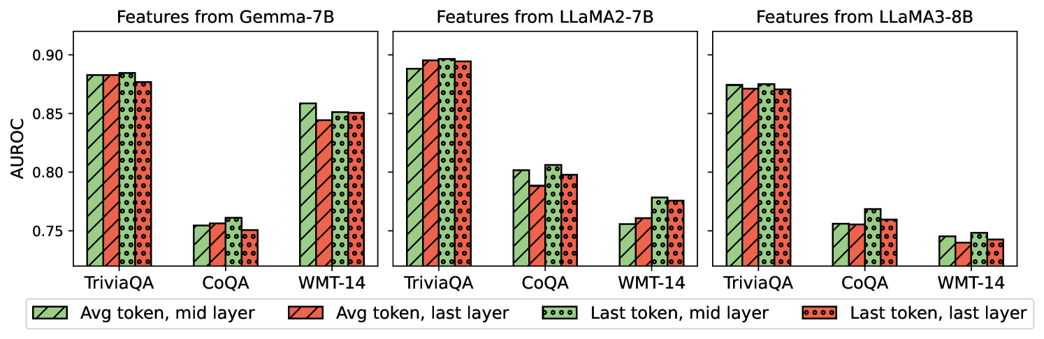### B.1 Layer comparison For general LLMs, each token is associated with a relatively large number of hidden layers (32 layers for LLaMA2-7B for example), each of which is represented by high-dimensional vectors (4096 for LLaMA2-7B). Thus it is generally not a good practice to incorporate all hidden layers as features for the uncertainty estimation due to this dimensionality. Previous works find that the middle layer and the last layer activations of the LLM’s last token contain the most useful features for supervised learning (Burns et al., 2022; Chen et al., 2024; Ahdritz et al., 2024; Azaria and Mitchell, 2023). To investigate the layer-wise effect for uncertainty estimation, we implement our Wb-S method with features different in two aspects: (i) different layers within the LLM architecture, specifically focusing on the middle and last layers (e.g., LLaMA2-7B and LLaMA3-8B: 16th and 32nd layers out of 32 layers with 4096 dimensions; Gemma-7B: 14th and 28th layers out of 28 layers with 3072 dimensions); and (ii) position of token activations, including averaging hidden activations over all the prompt/answer tokens or utilizing the hidden activation of the last token. The second aspect makes sense when the output contains more than one token, so we conduct this experiment on the natural language generation tasks only. Figure 3 gives a visualization of the comparison result. While the performances of these different feature extraction ways are quite similar in terms of performance across different tasks and LLMs, activation features from the middle layer generally perform better than the last layer. This may come from the fact that the last layer focuses more on the generation of the next token instead of summarizing information of the whole sentence, as has been discussed by Azaria and Mitchell (2023). <details> <summary>x3.png Details</summary>  ### Visual Description ## Bar Chart: AUROC Comparison Across Models and Features ### Overview The image is a grouped bar chart comparing the Area Under the Receiver Operating Characteristic curve (AUROC) for three language models (Gemma-7B, LLaMA2-7B, LLaMA3-8B) across three datasets (TriviaQA, CoQA, WMT-14). Four feature extraction methods are compared: 1. **Avg token, mid layer** (solid green) 2. **Avg token, last layer** (striped red) 3. **Last token, mid layer** (dotted green) 4. **Last token, last layer** (dotted red) ### Components/Axes - **X-axis**: Datasets (TriviaQA, CoQA, WMT-14) - **Y-axis**: AUROC values (0.75–0.90) - **Legend**: Located at the bottom, mapping colors/patterns to feature extraction methods. - **Model Sections**: Three vertical groupings (left: Gemma-7B, center: LLaMA2-7B, right: LLaMA3-8B). ### Detailed Analysis #### Gemma-7B - **TriviaQA**: - Avg token, mid layer: ~0.88 - Avg token, last layer: ~0.87 - Last token, mid layer: ~0.88 - Last token, last layer: ~0.87 - **CoQA**: - Avg token, mid layer: ~0.76 - Avg token, last layer: ~0.76 - Last token, mid layer: ~0.77 - Last token, last layer: ~0.75 - **WMT-14**: - Avg token, mid layer: ~0.86 - Avg token, last layer: ~0.85 - Last token, mid layer: ~0.86 - Last token, last layer: ~0.85 #### LLaMA2-7B - **TriviaQA**: - Avg token, mid layer: ~0.89 - Avg token, last layer: ~0.89 - Last token, mid layer: ~0.89 - Last token, last layer: ~0.89 - **CoQA**: - Avg token, mid layer: ~0.80 - Avg token, last layer: ~0.79 - Last token, mid layer: ~0.81 - Last token, last layer: ~0.80 - **WMT-14**: - Avg token, mid layer: ~0.77 - Avg token, last layer: ~0.76 - Last token, mid layer: ~0.78 - Last token, last layer: ~0.77 #### LLaMA3-8B - **TriviaQA**: - Avg token, mid layer: ~0.88 - Avg token, last layer: ~0.87 - Last token, mid layer: ~0.88 - Last token, last layer: ~0.87 - **CoQA**: - Avg token, mid layer: ~0.76 - Avg token, last layer: ~0.75 - Last token, mid layer: ~0.77 - Last token, last layer: ~0.75 - **WMT-14**: - Avg token, mid layer: ~0.74 - Avg token, last layer: ~0.73 - Last token, mid layer: ~0.75 - Last token, last layer: ~0.74 ### Key Observations 1. **TriviaQA Dominance**: All models achieve highest AUROC on TriviaQA, suggesting it is the most discriminative dataset. 2. **Feature Method Trends**: - **Avg token, mid layer** consistently outperforms other methods across models. - **Last token, last layer** underperforms compared to other feature combinations. 3. **Model Performance**: - LLaMA2-7B achieves the highest AUROC values overall. - LLaMA3-8B and Gemma-7B show similar performance, with LLaMA3-8B slightly trailing in CoQA/WMT-14. 4. **Dataset Variance**: CoQA and WMT-14 exhibit lower AUROC values, indicating weaker model performance on these tasks. ### Interpretation The data suggests that **TriviaQA** is the most effective dataset for evaluating these models, likely due to its focus on factual knowledge. Feature extraction methods involving **average token representations from mid layers** yield the best results, implying that distributed semantic information (rather than isolated tokens or late-layer features) is critical for performance. Larger models (e.g., LLaMA3-8B) outperform smaller ones, but the gap narrows in CoQA/WMT-14, where all models struggle. The underperformance of "last token, last layer" features may indicate overfitting or reduced generalization in late-layer representations. ### Spatial Grounding - **Legend**: Bottom-center, aligned with x-axis labels. - **Model Sections**: Vertically stacked, with Gemma-7B (left), LLaMA2-7B (center), LLaMA3-8B (right). - **Bar Order**: Within each model section, bars are ordered left-to-right as TriviaQA, CoQA, WMT-14. ### Component Isolation - **Header**: Model titles (Gemma-7B, LLaMA2-7B, LLaMA3-8B) above each section. - **Main Chart**: Grouped bars for datasets and feature methods. - **Footer**: AUROC axis (y-axis) and dataset labels (x-axis). ### Content Details - **TriviaQA Bars**: Tallest across all models, with AUROC values clustered near 0.88–0.89. - **CoQA Bars**: Shortest, with values ~0.75–0.81. - **WMT-14 Bars**: Intermediate, ~0.74–0.86. ### Notable Anomalies - **LLaMA2-7B CoQA**: Last token, mid layer (dotted green) slightly outperforms avg token, last layer (striped red), contradicting the general trend. - **LLaMA3-8B WMT-14**: Avg token, mid layer (solid green) is marginally better than last token, mid layer (dotted green), but the difference is minimal (~0.74 vs. ~0.75). This analysis highlights the importance of dataset selection and feature extraction strategy in model evaluation, with TriviaQA and mid-layer average tokens emerging as optimal choices. </details> Figure 3: Performance comparison of using hidden activations from different tokens and layers as features in the Wb-S method. The bars filled with ‘/’ and ‘.’ represent the activations averaged over the answer tokens and the hidden activation of the last token, respectively. And the green and orange bars denote the activations from the middle and the last layer, respectively. ### B.2 Scaling effect In Figure 4, we investigate whether larger LLMs’ hidden activations enhance our uncertainty estimation method. For a fair comparison, we fix the target LLM that generates the output in Algorithm 1 and vary the tool LLM used for analysis. For example, in the left plot of Figure 4, we use Gemma-7B to generate the outputs, and LLaMA2-7B, LLaMA2-13B, and Gemma-7B to perform uncertainty estimation. <details> <summary>x4.png Details</summary>  ### Visual Description ## Bar Chart: Model Performance Comparison Across Tasks and Scenarios ### Overview The image contains three grouped bar charts comparing the performance of four models (Wb-S, Gb-S, 7B, 13B) across four tasks (MMLU, TriviaQA, CoQA, WMT-14) in three scenarios: 1. **Use LLaMA2 to predict Gemma-7B** 2. **Use Gemma to predict LLaMA2-7B** 3. **Use Gemma to predict LLaMA3-8B** Performance is measured using the **AUROC metric** (0.7–1.0 scale). --- ### Components/Axes - **X-Axis**: Tasks (MMLU, TriviaQA, CoQA, WMT-14) - **Y-Axis**: AUROC (0.7–1.0) - **Legend**: - **Wb-S**: White bars - **Gb-S**: Gray bars - **7B**: Green bars with diagonal hatching - **13B**: Red bars with dotted patterns - **Chart Titles**: Positioned at the top of each subplot. - **Bar Grouping**: Each task has four bars (one per model), grouped by task. --- ### Detailed Analysis #### **1. Use LLaMA2 to predict Gemma-7B** - **MMLU**: - Wb-S: ~0.84 | Gb-S: ~0.83 | 7B: ~0.84 | 13B: ~0.84 - **TriviaQA**: - Wb-S: ~0.88 | Gb-S: ~0.87 | 7B: ~0.88 | 13B: ~0.90 - **CoQA**: - Wb-S: ~0.76 | Gb-S: ~0.74 | 7B: ~0.75 | 13B: ~0.76 - **WMT-14**: - Wb-S: ~0.86 | Gb-S: ~0.84 | 7B: ~0.86 | 13B: ~0.85 #### **2. Use Gemma to predict LLaMA2-7B** - **MMLU**: - Wb-S: ~0.72 | Gb-S: ~0.72 | 7B: ~0.72 | 13B: ~0.72 - **TriviaQA**: - Wb-S: ~0.90 | Gb-S: ~0.82 | 7B: ~0.85 | 13B: ~0.92 - **CoQA**: - Wb-S: ~0.80 | Gb-S: ~0.05 (outlier) | 7B: ~0.78 | 13B: ~0.85 - **WMT-14**: - Wb-S: ~0.78 | Gb-S: ~0.72 | 7B: ~0.76 | 13B: ~0.79 #### **3. Use Gemma to predict LLaMA3-8B** - **MMLU**: - Wb-S: ~0.83 | Gb-S: ~0.83 | 7B: ~0.83 | 13B: ~0.83 - **TriviaQA**: - Wb-S: ~0.87 | Gb-S: ~0.86 | 7B: ~0.78 | 13B: ~0.84 - **CoQA**: - Wb-S: ~0.77 | Gb-S: ~0.74 | 7B: ~0.73 | 13B: ~0.74 - **WMT-14**: - Wb-S: ~0.74 | Gb-S: ~0.72 | 7B: ~0.68 | 13B: ~0.70 --- ### Key Observations 1. **Consistency Across Scenarios**: - Wb-S and Gb-S show relatively stable performance across tasks and scenarios. - 7B and 13B models exhibit task-specific variability. 2. **Outliers**: - **Gb-S in CoQA (Scenario 2)**: AUROC drops to ~0.05, suggesting a critical failure or overfitting. - **7B in WMT-14 (Scenario 3)**: AUROC plummets to ~0.68, indicating poor generalization. 3. **Trends**: - **Larger Models (13B)**: Outperform smaller models in TriviaQA (Scenario 1 and 2) but underperform in CoQA (Scenario 3). - **Gemma’s Effectiveness**: Varies by target model size. For example, Gemma predicts LLaMA2-7B better than LLaMA3-8B in TriviaQA. --- ### Interpretation - **Model Generalization**: - Wb-S and Gb-S demonstrate robustness across tasks, while 7B and 13B models show task-dependent performance. - The 13B model excels in TriviaQA (Scenario 1 and 2) but struggles in CoQA (Scenario 3), suggesting over-reliance on specific training data. - **Gemma’s Role**: - Gemma’s predictive accuracy depends on the target model’s architecture. For instance, it performs better with LLaMA2-7B in TriviaQA but worse with LLaMA3-8B in CoQA. - **Anomalies**: - The extreme drop in Gb-S (Scenario 2, CoQA) highlights potential instability in smaller models under certain prediction scenarios. - **Practical Implications**: - Larger models (13B) may not always outperform smaller ones, emphasizing the need for task-specific tuning. - Gemma’s utility as a predictor is context-dependent, requiring careful model selection based on the target architecture. </details> Figure 4: (Left) Using the hidden activations of LLaMA2-7B and LLaMA2-13B to estimate the uncertainty of the answer provided by Gemma-7B. (Middle) Using the hidden activations of Gemma-2B and Gemma-7B to estimate the uncertainty of the answer provided by LLaMA2-7B. (Right) Using the hidden activations of Gemma-2B and Gemma-7B to estimate the uncertainty of the answer provided by LLaMA3-8B We find that larger LLM does encode better knowledge about the uncertainty, which is attributed to their improved knowledge in answering the questions. We also note that in the case of using Gemma to predict LLaMA2-7B, even a small tool LLM (Gemma-2B) is capable of achieving better performance than the Gb-S that only uses the entropy- and probability-related features from the target LLM. This result also underscores the benefits of adopting the internal state in estimating the uncertainty, even from an LLM different from the one generating the answers. ### B.3 Histogram of correlations Figure 5 plots the histograms of the pairwise correlations between the neuron activations and the labels (whether the LLM’s response is correct). We make two observations here: First, for both LLMs, some neurons have a significantly positive (or negative) correlation with the label. We can interpret these neurons as the uncertainty neuron for the corresponding task. When these neurons are activated, the LLMs are uncertain about their responses. Second, Gemma-7B and LLaMA3-8B have more significant neurons than LLaMA2-7B, and this is consistent with the better performance of Gemma-7B and LLaMA3-8B in Table 1 and Table 2. Also, this reinforces that the hidden activations of the LLMs contain uncertainty information about the LLM’s output. 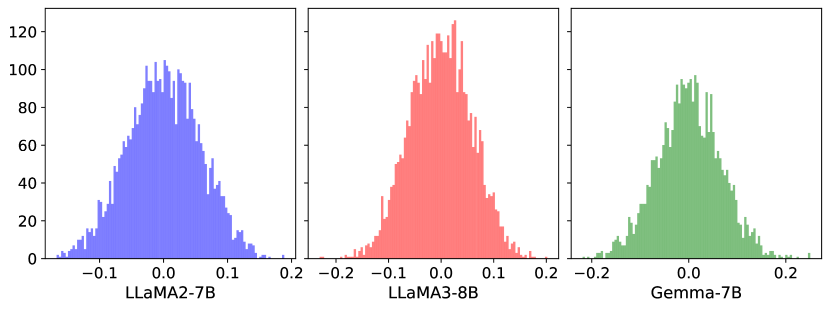<details> <summary>x5.png Details</summary>  ### Visual Description ## Histograms: Model Performance Distributions ### Overview The image displays three side-by-side histograms comparing distributions of a metric (likely model performance) across three language models: LLaMA2-7B (blue), LLaMA3-8B (red), and Gemma-7B (green). Each histogram shows frequency counts (y-axis) against a normalized scale (-0.2 to 0.2) on the x-axis. ### Components/Axes - **X-Axes**: - LLaMA2-7B: Range -0.2 to 0.2 - LLaMA3-8B: Range -0.2 to 0.2 - Gemma-7B: Range -0.2 to 0.2 - **Y-Axes**: - All histograms share a "Count" axis (0 to 120) - **Legend**: - Top-center placement - Blue = LLaMA2-7B - Red = LLaMA3-8B - Green = Gemma-7B ### Detailed Analysis 1. **LLaMA2-7B (Blue)**: - Peak frequency: ~100 at x=0.0 - Symmetric distribution with gradual decline toward ±0.1 - Tails extend to ±0.15 with minimal counts 2. **LLaMA3-8B (Red)**: - Peak frequency: ~120 at x=0.0 - Narrower distribution than LLaMA2-7B - Declines sharply to ~40 at ±0.1 3. **Gemma-7B (Green)**: - Peak frequency: ~100 at x=0.0 - Broader spread than LLaMA3-8B but narrower than LLaMA2-7B - Tails reach ±0.18 with low counts ### Key Observations - All distributions are bell-shaped and symmetric, suggesting normal-like distributions. - LLaMA3-8B has the highest peak frequency (120), indicating a higher concentration of values near 0.0. - Gemma-7B exhibits the widest spread (up to ±0.18), while LLaMA3-8B is the most concentrated (peaks at ±0.1). - LLaMA2-7B shows intermediate spread and frequency. ### Interpretation The histograms likely represent a performance metric (e.g., accuracy, error rate) normalized to a common scale. LLaMA3-8B's higher peak frequency suggests superior performance or consistency in the measured metric compared to the other models. The symmetry implies balanced performance across positive and negative deviations from the mean (0.0). Gemma-7B's broader distribution may indicate greater variability in outcomes, while LLaMA2-7B balances moderate spread and frequency. These patterns could reflect differences in model architecture, training data, or optimization strategies. 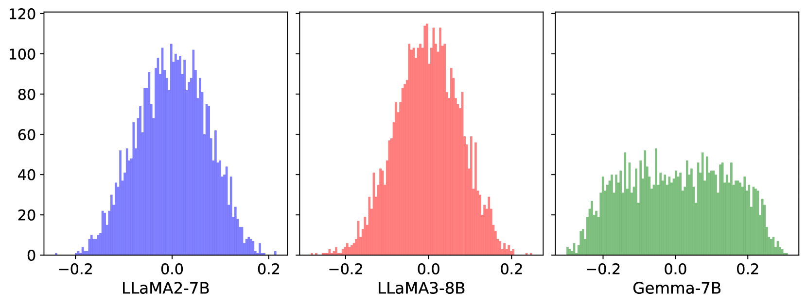</details> <details> <summary>x6.png Details</summary>  ### Visual Description ## Histograms: Distribution of Model Parameters ### Overview The image displays three histograms comparing the distribution of parameter values across three language models: LLaMA2-7B (blue), LLaMA3-8B (red), and Gemma-7B (green). Each histogram spans an x-axis range of -0.2 to 0.2 and a y-axis range of 0 to 120. The distributions vary significantly in peak height and spread. ### Components/Axes - **X-axis**: Labeled with numerical values from -0.2 to 0.2, representing parameter values. - **Y-axis**: Labeled with numerical values from 0 to 120, representing frequency counts. - **Legends**: - Blue: LLaMA2-7B - Red: LLaMA3-8B - Green: Gemma-7B - **Placement**: Legends are positioned directly below each histogram for spatial grounding. ### Detailed Analysis 1. **LLaMA2-7B (Blue)**: - **Peak**: ~100 at x = 0.0. - **Spread**: Symmetrical distribution with tails extending to ±0.15. - **Notable**: Sharp drop-off at ±0.15, with minimal values beyond this range. 2. **LLaMA3-8B (Red)**: - **Peak**: ~110 at x = 0.0. - **Spread**: Narrower than LLaMA2-7B, with tails reaching ±0.12. - **Notable**: Steeper decline near the peak, indicating a more concentrated distribution. 3. **Gemma-7B (Green)**: - **Peak**: ~80 at x = 0.0. - **Spread**: Broader distribution, with tails extending to ±0.2. - **Notable**: Flatter peak and more uniform distribution across the x-axis range. ### Key Observations - **Peak Heights**: LLaMA3-8B > LLaMA2-7B > Gemma-7B. - **Spread**: Gemma-7B exhibits the widest distribution, while LLaMA3-8B is the most concentrated. - **Symmetry**: LLaMA2-7B and LLaMA3-8B show near-symmetrical distributions, whereas Gemma-7B has a slight rightward skew. ### Interpretation The data suggests differences in parameter distribution among the models: - **LLaMA3-8B** likely has a more optimized or constrained parameter space, reflected in its narrow, high-peak distribution. - **Gemma-7B**'s broader spread may indicate greater variability in parameter initialization or training dynamics. - The symmetry of LLaMA2-7B and LLaMA3-8B implies balanced training objectives, while Gemma-7B's asymmetry could point to architectural or methodological differences. These trends highlight how model architecture, training data, or hyperparameters influence parameter distribution, which may correlate with performance or efficiency metrics not shown here. </details> Figure 5: The histograms of the pairwise correlations on the TriviaQA task between the neuron activations and the labels (whether the LLM’s response is correct), where the neural values are the last-token hidden activations of answers from the middle layer (upper) and the last layer (lower) of two models respectively. Figure 6 plots some example neurons’ activation by selecting the neurons with the largest absolute correlations in Figure 5. More neurons from the last layer can be found in Figure 7. These neurons as an individual indicator exhibit different distributional patterns when the response is correct compared to when the response is incorrect, and thus reflect the uncertainty of the LLM’s responses. 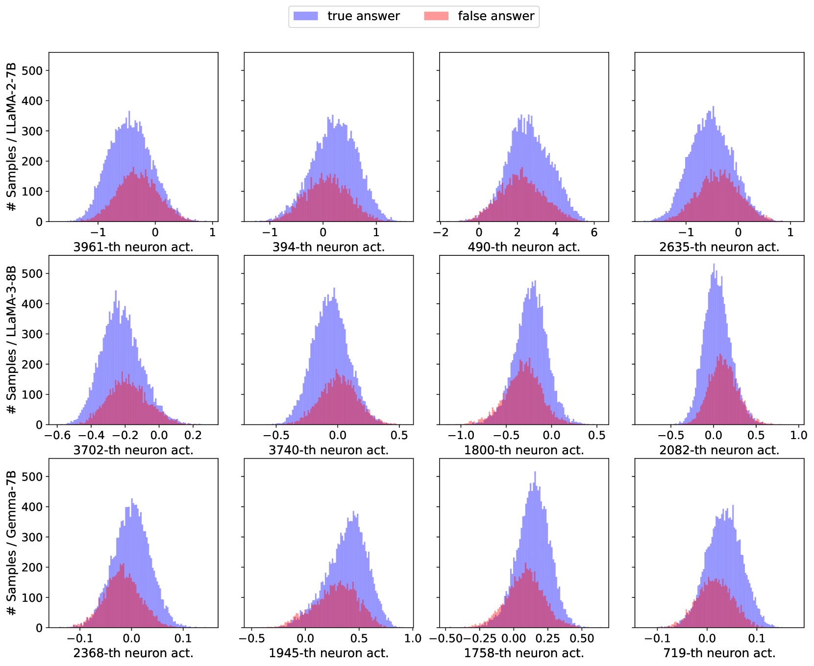<details> <summary>x7.png Details</summary>  ### Visual Description ## Histogram Grid: Neuron Activation Distributions for True vs. False Answers ### Overview The image displays a 4x3 grid of histograms comparing neuron activation distributions for "true answer" (blue) and "false answer" (red) classifications. Each histogram represents a specific neuron (e.g., 3961-th, 394-th, etc.) and shows the frequency of activation values across samples. The y-axis represents normalized sample counts divided by two language models (LLaMA-2-7B and Gemma-7B), while the x-axis shows activation value ranges. ### Components/Axes - **Legend**: Positioned at the top-center, with: - Blue = True answer - Red = False answer - **Y-axis**: - Title: "# Samples / LLaMA-2-7B" (top row) or "# Samples / Gemma-7B" (bottom row) - Scale: 0 to 500 (top row) or 0 to 400 (bottom row) - **X-axis**: - Titles: "neuron act." (activation values) - Ranges vary by neuron: - Top row: -1 to 1 (3961-th), -1 to 1 (394-th), -2 to 6 (490-th), -1 to 1 (2635-th) - Middle row: -0.6 to 0.2 (3702-th), -0.5 to 0.5 (3740-th), -0.5 to 0.5 (1800-th), -0.5 to 0.5 (1758-th) - Bottom row: -0.1 to 0.1 (2368-th), -0.5 to 0.5 (1945-th), -0.1 to 0.1 (2082-th), -0.1 to 0.1 (719-th) ### Detailed Analysis 1. **3961-th neuron act.** (Top-left): - X-axis: -1 to 1 - Blue peak: ~0.0 (height ~300 samples) - Red peak: ~0.1 (height ~200 samples) - Overlap: Significant between -0.2 and 0.2 2. **394-th neuron act.** (Top-center): - X-axis: -1 to 1 - Blue peak: ~0.0 (height ~400 samples) - Red peak: ~0.3 (height ~250 samples) - Separation: Moderate (0.3 difference) 3. **490-th neuron act.** (Top-right): - X-axis: -2 to 6 - Blue peak: ~2.0 (height ~350 samples) - Red peak: ~4.0 (height ~220 samples) - Wide spread: Blue spans -1 to 3, Red spans 1 to 5 4. **2635-th neuron act.** (Middle-left): - X-axis: -1 to 1 - Blue peak: ~-0.5 (height ~320 samples) - Red peak: ~0.0 (height ~280 samples) - Overlap: Strong between -0.5 and 0.5 5. **3702-th neuron act.** (Middle-center): - X-axis: -0.6 to 0.2 - Blue peak: ~-0.2 (height ~380 samples) - Red peak: ~0.0 (height ~260 samples) - Narrow range: Both distributions confined to -0.6 to 0.2 6. **3740-th neuron act.** (Middle-right): - X-axis: -0.5 to 0.5 - Blue peak: ~0.0 (height ~410 samples) - Red peak: ~0.2 (height ~290 samples) - Symmetric spread: Both distributions centered near 0 7. **1800-th neuron act.** (Bottom-left): - X-axis: -0.5 to 0.5 - Blue peak: ~-0.3 (height ~360 samples) - Red peak: ~0.1 (height ~270 samples) - Overlap: Moderate between -0.3 and 0.1 8. **1758-th neuron act.** (Bottom-center): - X-axis: -0.5 to 0.5 - Blue peak: ~0.0 (height ~430 samples) - Red peak: ~0.4 (height ~300 samples) - Clear separation: 0.4 difference between peaks 9. **2368-th neuron act.** (Bottom-right): - X-axis: -0.1 to 0.1 - Blue peak: ~0.0 (height ~390 samples) - Red peak: ~0.05 (height ~250 samples) - Minimal spread: Both distributions tightly clustered ### Key Observations 1. **Peak Separation**: - Neurons 490-th and 1758-th show the largest separation between true/false peaks (0.4 and 0.3 activation differences). - Neurons 3961-th and 2368-th show the smallest separation (<0.1 activation difference). 2. **Distribution Width**: - 490-th neuron has the widest spread (6 units on x-axis). - 2368-th neuron has the narrowest spread (0.2 units on x-axis). 3. **Model Consistency**: - Top row (LLaMA-2-7B) shows broader distributions than bottom row (Gemma-7B). - Bottom row histograms generally have tighter activation ranges. ### Interpretation The histograms reveal that certain neurons (e.g., 490-th, 1758-th) exhibit strong discriminative power between true/false answers, with distinct activation peaks. Neurons with overlapping distributions (e.g., 3961-th, 2368-th) likely play less direct roles in answer classification. The tighter distributions in Gemma-7B samples suggest more consistent neuron behavior compared to LLaMA-2-7B. These patterns align with findings in neural network interpretability studies, where specific neurons often encode distinct semantic features critical for task performance. </details> Figure 6: Distribution of values from particular neurons of mid-layers on TriviaQA dataset. 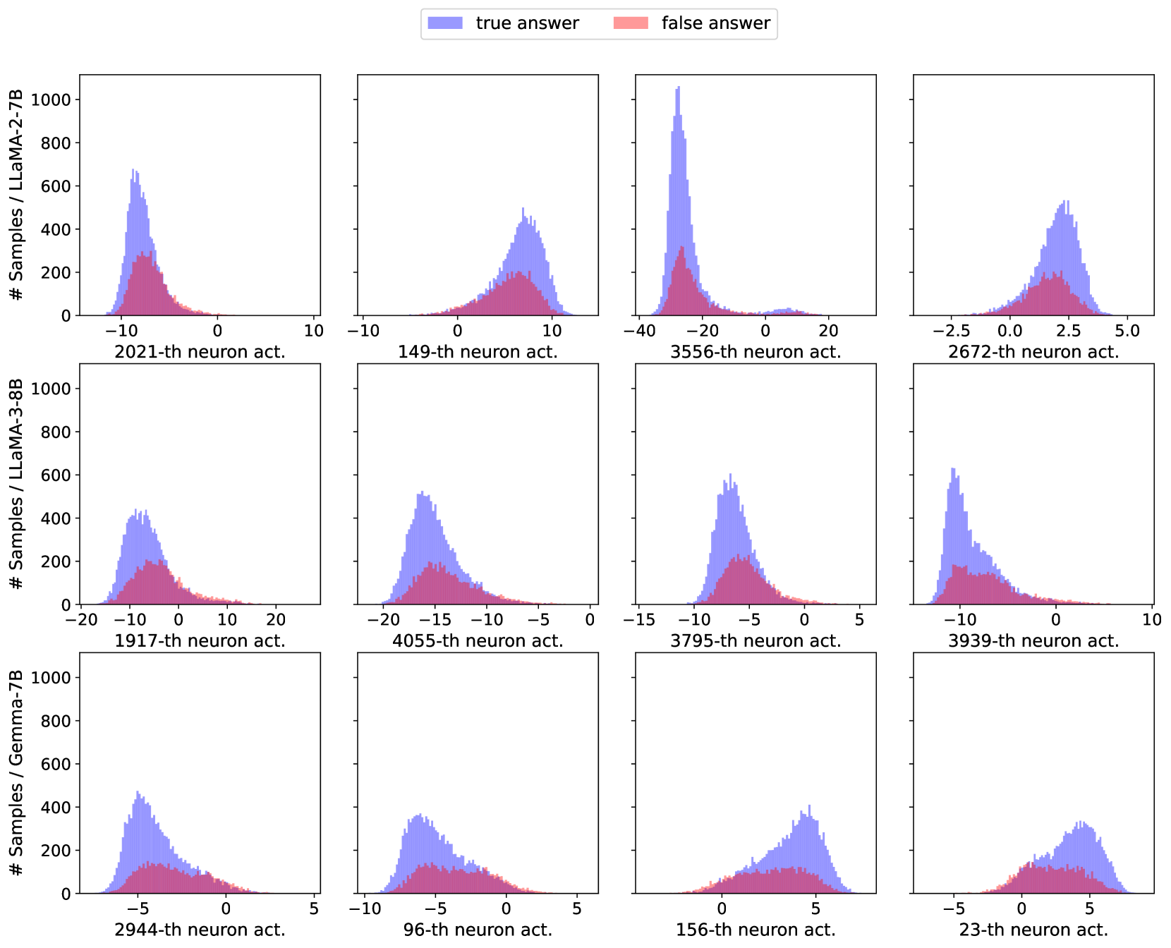<details> <summary>x8.png Details</summary>  ### Visual Description ## Grid of Histograms: Neuron Activity Distributions for True vs. False Answers ### Overview The image displays a 4x3 grid of histograms comparing neuron activity distributions for "true answer" (blue) and "false answer" (red) classifications. Each subplot corresponds to a specific neuron (e.g., "2021-th neuron act.") and visualizes the frequency of neuron activation values across samples. The histograms are normalized to show counts on the y-axis, with x-axis ranges varying per neuron. ### Components/Axes - **Legend**: Located at the top center, with: - **Blue**: True answer - **Red**: False answer - **X-axis**: Labeled "Neuron act." with ranges varying per subplot (e.g., -10 to 10, -40 to 20, -15 to 5). - **Y-axis**: Labeled "# Samples / LLaMA-2-7B" for the first three rows and "# Samples / Gemma-7B" for the last row. Scales range from 0 to 1000. - **Subplot Titles**: Each histogram is labeled with the neuron number (e.g., "2021-th neuron act."). ### Detailed Analysis 1. **2021-th neuron act.**: - X-axis: -10 to 10 - Blue peak: ~0 (count ~600) - Red peak: ~-5 (count ~300) 2. **149-th neuron act.**: - X-axis: -10 to 10 - Blue peak: ~0 (count ~500) - Red peak: ~-10 (count ~200) 3. **3556-th neuron act.**: - X-axis: -40 to 20 - Blue peak: ~0 (count ~800) - Red peak: ~-20 (count ~100) 4. **2672-th neuron act.**: - X-axis: -15 to 5 - Blue peak: ~-10 (count ~400) - Red peak: ~-15 (count ~150) 5. **1917-th neuron act.**: - X-axis: -5 to 5 - Blue peak: ~0 (count ~450) - Red peak: ~-5 (count ~200) 6. **4055-th neuron act.**: - X-axis: -10 to 10 - Blue peak: ~-5 (count ~550) - Red peak: ~-10 (count ~250) 7. **3795-th neuron act.**: - X-axis: -5 to 5 - Blue peak: ~5 (count ~600) - Red peak: ~0 (count ~300) 8. **2944-th neuron act.**: - X-axis: -10 to 10 - Blue peak: ~0 (count ~500) - Red peak: ~-5 (count ~250) 9. **96-th neuron act.**: - X-axis: -10 to 10 - Blue peak: ~-5 (count ~450) - Red peak: ~-10 (count ~200) 10. **156-th neuron act.**: - X-axis: -5 to 5 - Blue peak: ~5 (count ~550) - Red peak: ~0 (count ~300) 11. **3939-th neuron act.**: - X-axis: -5 to 5 - Blue peak: ~5 (count ~600) - Red peak: ~0 (count ~300) 12. **23-th neuron act.**: - X-axis: -5 to 5 - Blue peak: ~5 (count ~550) - Red peak: ~0 (count ~300) ### Key Observations - **Peak Activity**: True answers (blue) generally show higher peak counts than false answers (red) across most neurons. - **X-axis Variability**: Neuron activity ranges differ significantly (e.g., 3556-th neuron spans -40 to 20, while others are narrower). - **Model-Specific Labels**: The last row uses "Gemma-7B" instead of "LLaMA-2-7B" for the y-axis, suggesting dataset/model differences. - **Outliers**: The 3556-th neuron has the highest blue peak (~800 samples), indicating a strong signal for true answers. ### Interpretation The histograms suggest that neuron activity patterns correlate with answer correctness. True answers often exhibit higher-frequency activation at specific values (e.g., near 0 or positive ranges), while false answers show lower or shifted peaks. The 3556-th neuron’s extreme blue peak implies it may be a critical feature for distinguishing correct responses. The shift in y-axis labels from LLaMA-2-7B to Gemma-7B in the final row hints at methodological changes or dataset variations between groups. These patterns could inform neural network interpretability or model debugging efforts. </details> Figure 7: More distribution of values from specific neurons of last layers on the TriviaQA dataset. The plots are obtained in the same way as Figure 6. ### B.4 Proof of Proposition 4.1 The proof of Proposition 4.1 follows from the definition of $f^{*}.$ ## Appendix C Calibration performance In Section 4.1, we distinguish the two tasks of uncertainty estimation and uncertainty calibration. Throughout the paper, we have been focused on improving the performance on the task of uncertainty estimation – to predict when the LLM is uncertain about its response. Generally, a better uncertainty estimation model leads to one with better calibration performance. The calibration (or recalibration) of the uncertainty estimation model can be indeed reduced to the classic ML setting which does not involve the LLM. Table 4 gives the calibration performance and we see an advantage of our supervised methods over benchmark methods consistent with the AUROC performance in Table 1. We adopt the histogram binning method here because we find that the temperature scaling method and the Platt scaling method will give all predicted scores concentrated within a small range such as $[0.2,0.6]$ . We also do not exclude the possibility that the other calibration methods can give even better performance. The point to make here is that uncertainty estimation and uncertainty calibration are two closely related tasks. Note that (i) a better uncertainty estimation model leads to a better calibration performance and (ii) the LLMs are pretrained and not designed for these NLP tasks in the first place (see Section 4.2) so that there is no uncertainty score readily available (as the predicted probabilities for the image classifiers); we emphasize the importance of an extra uncertainty estimation procedure as our supervised one so to extract the uncertainty information from the inside of the LLMs. | NLL | TriviaQA | G-7B | 0.478 | 0.500 | 0.428 | 0.472 | 0.739 | 8.710 | 0.414 | 0.467 | 0.392 | | --- | --- | --- | --- | --- | --- | --- | --- | --- | --- | --- | --- | | L-7B | 1.155 | 0.551 | 0.575 | 0.600 | 1.481 | 21.119 | 0.338 | 0.580 | 0.388 | | | | L-8B | 0.483 | 0.407 | 0.383 | 0.401 | 0.719 | 8.515 | 0.423 | 0.467 | 0.365 | | | | CoQA | G-7B | 0.778 | 0.474 | 0.469 | 0.476 | 0.632 | 8.106 | 0.474 | 0.497 | 0.457 | | | L-7B | 1.047 | 0.620 | 0.637 | 0.649 | 1.358 | 11.708 | 0.417 | 0.607 | 0.457 | | | | L-8B | 0.823 | 0.502 | 0.508 | 0.499 | 0.762 | 8.007 | 0.551 | 0.535 | 0.507 | | | | WMT-14 | G-7B | 9.674 | 1.266 | 0.809 | 0.618 | 0.701 | 17.933 | 0.454 | 0.463 | 0.449 | | | L-7B | 1.204 | 1.150 | 0.718 | 0.809 | 0.796 | 16.913 | 0.553 | 0.622 | 0.583 | | | | L-8B | 1.490 | 0.752 | 0.652 | 0.676 | 0.722 | 21.340 | 0.649 | 0.673 | 0.612 | | | | ECE | TriviaQA | G-7B | 0.152 | 0.138 | 0.066 | 0.115 | 0.275 | 0.253 | 0.056 | 0.075 | 0.067 | | L-7B | 0.437 | 0.068 | 0.048 | 0.146 | 0.188 | 0.616 | 0.043 | 0.087 | 0.049 | | | | L-8B | 0.171 | 0.082 | 0.046 | 0.081 | 0.196 | 0.283 | 0.107 | 0.087 | 0.075 | | | | CoQA | G-7B | 0.356 | 0.054 | 0.112 | 0.064 | 0.221 | 0.237 | 0.121 | 0.129 | 0.113 | | | L-7B | 0.397 | 0.065 | 0.105 | 0.073 | 0.174 | 0.494 | 0.052 | 0.071 | 0.038 | | | | L-8B | 0.339 | 0.031 | 0.071 | 0.033 | 0.196 | 0.312 | 0.156 | 0.110 | 0.122 | | | | WMT-14 | G-7B | 0.499 | 0.464 | 0.234 | 0.197 | 0.072 | 0.521 | 0.097 | 0.063 | 0.073 | | | L-7B | 0.164 | 0.389 | 0.065 | 0.269 | 0.127 | 0.491 | 0.045 | 0.090 | 0.101 | | | | L-8B | 0.318 | 0.192 | 0.051 | 0.142 | 0.029 | 0.618 | 0.145 | 0.201 | 0.137 | | | | Brier | TriviaQA | G-7B | 0.282 | 0.221 | 0.224 | 0.215 | 0.344 | 0.279 | 0.266 | 0.288 | 0.282 | | L-7B | 0.431 | 0.241 | 0.271 | 0.259 | 0.322 | 0.645 | 0.334 | 0.322 | 0.315 | | | | L-8B | 0.262 | 0.192 | 0.204 | 0.188 | 0.291 | 0.373 | 0.258 | 0.265 | 0.255 | | | | CoQA | G-7B | 0.318 | 0.174 | 0.188 | 0.171 | 0.232 | 0.241 | 0.207 | 0.218 | 0.212 | | | L-7B | 0.395 | 0.233 | 0.242 | 0.230 | 0.265 | 0.464 | 0.296 | 0.256 | 0.276 | | | | L-8B | 0.338 | 0.197 | 0.201 | 0.191 | 0.255 | 0.359 | 0.258 | 0.242 | 0.248 | | | | WMT-14 | G-7B | 0.505 | 0.454 | 0.330 | 0.319 | 0.247 | 0.606 | 0.327 | 0.287 | 0.309 | | | L-7B | 0.313 | 0.413 | 0.271 | 0.334 | 0.275 | 0.502 | 0.296 | 0.277 | 0.288 | | | | L-8B | 0.343 | 0.279 | 0.250 | 0.263 | 0.246 | 0.620 | 0.282 | 0.300 | 0.284 | | | Table 4: Calibration performance on natural language generation tasks after histogram binning. The base models are from Table 1. The original uncertainty scores from the base models are first scaled into $[0,1]$ and then a histogram binning is performed with 20 bins of equal length. ## Appendix D Details for the Numerical Experiments We ran all of our experiments on an AMD EPYC 7452 128-core processor with 4 $\times$ 48G NVIDIA A6000 GPUs. ### D.1 Dataset preparation In the following we provide more information for the three tasks considered in our numerical experiments. - Question answering. We follow Kuhn et al. (2023) and use the CoQA and TriviaQA (Joshi et al., 2017) datasets. The CoQA task requires the LLM to answer questions by understanding the provided text, and the TriviaQA requires the LLM to answer questions based on its pre-training knowledge. We adopt the scoring function $s(\cdot,\cdot)$ as Rouge-1 (Lin and Och, 2004a) and label a response $\bm{y}_{i}$ as correct if $s(\bm{y}_{i},\bm{y}_{i,\text{true}})\geq 0.3$ and incorrect otherwise. - Multiple choice. We consider the Massive Multitask Language Understanding (MMLU) dataset (Hendrycks et al., 2020), a collection of 15,858 questions covering 57 subjects across STEM. Due to the special structure of the dataset, the generated output $\bm{y}_{i}$ and the correct answer $\bm{y}_{\text{true},i}\in\{\text{A, B, C, D}\}$ . Therefore, this task can also be regarded as a classification problem for the LLM by answering the question with one of the four candidate choices. - Machine translation. We consider the WMT 2014 dataset (Bojar et al., 2014) for estimating LLM’s uncertainty on the machine translation task. The scoring function $s(\cdot,\cdot)$ is chosen to be the BLEU score (Papineni et al., 2002; Lin and Och, 2004b) and the generated answer $\bm{y}_{i}$ is labeled as correct if $s(\bm{y}_{i},\bm{y}_{i,\text{true}})>0.3$ and incorrect otherwise. Prompt dataset generation. For all the tasks studied in this paper, we adopt the few-shot prompting for the LLM. Specifically, in the prompt, we provide $r$ examples to make the LLM learn the format of the response, as illustrated in the following. For the question-answering task, we construct the prompt without using any question-answering sample repeatedly in the original dataset. For example, Prompt 1 includes the 1st to $r$ -th question-answering samples in the original dataset as the examples and the $(r+1)$ -th sample as the target question-answering pair for the LLM; next, Prompt 2 uses the $(r+2)$ -th to $(2r+1)$ -th samples as the examples and the $(2r+2)$ -th sample as the target question-answering pair. However, as the test datasets of MMLU and WMT used for evaluation are not sufficiently large, we generate the prompt in a convolution-like manner: Prompt 2 includes the 2nd to $(r+1)$ -th question-answering samples as the examples and the $(r+2)$ -th sample as the target question-answering pair. Dataset split. After generating the prompt-answering dataset, we split this dataset into two parts for training the calibration model and evaluation/test. For the MMLU and WMT datasets, we take the dataset generated from the original validation/test dataset. For the question-answering task, as the answer of TriviaQA in the original test dataset is vacant, we take the first 2000 generated prompt-answering pairs from the training dataset as the test dataset, and the remaining for training. Prompting format. Here we give the different prompting templates used for different tasks. We use few-shot prompting and the templates can always be roughly divided into four parts: introduction (empty only for WMT), examples, question, and answer, where examples are just $r$ distinct question-answer pairs in the same form as the question and answer parts. We feed the model with the template string except for the reference answer as inputs. COQA Reading the passage and answer given questions accordingly. Passage: {a passage in COQA} Examples: {r distinct QA pairs related to the given passage} Q: {a new question related to the given passage} A: {reference answer} TriviaQA Answer the question as following examples. Examples: {r distinct QA pairs} Q: {a new question} A: {reference answer} MMLU You would be given a multiple-choice question paired with 4 choices (A-D). Choose one of them using letter A, B, C, or D as the correct answer to the question. Here are some examples: {r distinct QA pairs} Now answer the question: {a new question} A: {answer sentence A} B: {answer sentence B} C: {answer sentence C} D: {answer sentence D} Answer: {reference answer (a letter)} WMT {r distinct QA pairs} Q: What is the English translation of the following sentence? {a French sentence} A: {reference answer (an English sentence)} ### D.2 Details of the training procedure For the three regimes of our supervised approach presented in Section 3.3, the details of the supervised training procedure are as below: Gb-S. For the natural language generation tasks (question-answering and machine-translation), we train a random forest model with the input features listed in Table 5 (20 features in total). For the multiple-choice task, as the answer has only one token from {A, B, C, D}, we take the output logits of these 4 tokens (denoted as $\alpha_{\text{A}}$ , $\alpha_{\text{B}}$ , $\alpha_{\text{C}}$ , and $\alpha_{\text{D}}$ ) after inputting the question prompt $\bm{x}$ to the LLM. Then, we get the probability of each choice as follows: $$ p_{\theta}(y|\bm{x})=\frac{\text{exp}(\alpha_{y})}{\sum_{y^{\prime}\in\{\text{ A},\text{B},\text{C},\text{D}\}}\text{exp}(\alpha_{y^{\prime}})},\ \forall y \in\{\text{A},\text{B},\text{C},\text{D}\}. $$ Then we use 5 features as the input to Gb-S: the entropy of this distribution, and the sorted probability values in descending order. | Max Ent Min Ent Avg Ent | $\max_{j\in\{1,...,m\}}\ H(p_{\theta}(\cdot|\bm{x},\bm{y}_{1:j-1}))$ $\min_{j\in\{1,...,m\}}\ H(p_{\theta}(\cdot|\bm{x},\bm{y}_{1:j-1}))$ $\frac{1}{m}\sum_{j=1}^{m}H(p_{\theta}(\cdot|\bm{x},\bm{y}_{1:j-1}))$ | $\max_{j\in\{1,...,n\}}\ H(p_{\theta}(\cdot|\bm{x}_{1:j-1}))$ $\min_{j\in\{1,...,n\}}\ H(p_{\theta}(\cdot|\bm{x}_{1:j-1}))$ $\frac{1}{n}\sum_{j=1}^{n}H(p_{\theta}(\cdot|\bm{x}_{1:j-1}))$ | | --- | --- | --- | | Std Ent | $\sqrt{\frac{\sum_{j=1}^{m}\left(H(p_{\theta}(\cdot|\bm{x},\bm{y}_{1:j-1}))- \text{Avg Ent}\right)^{2}}{m-1}}$ | $\sqrt{\frac{\sum_{j=1}^{n}\left(H(p_{\theta}(\cdot|\bm{x}_{1:j-1}))-\text{Avg Ent}\right)^{2}}{n-1}}$ | | Max Likelihood | $\max_{j\in\{1,...,m\}}\ -\log p_{\theta}(y_{j}|\bm{x},\bm{y}_{1:j-1})$ | $\max_{j\in\{1,...,n\}}\ -\log p_{\theta}(x_{j}|\bm{x}_{1:j-1})$ | | Min Likelihood | $\min_{j\in\{1,...,m\}}\ -\log p_{\theta}(y_{j}|\bm{x},\bm{y}_{1:j-1})$ | $\min_{j\in\{1,...,n\}}\ -\log p_{\theta}(x_{j}|\bm{x}_{1:j-1})$ | | Avg Likelihood | $\frac{1}{m}\sum_{j=1}^{m}-\log p_{\theta}(y_{j}|\bm{x},\bm{y}_{1:j-1})$ | $\frac{1}{n}\sum_{j=1}^{n}-\log p_{\theta}(x_{j}|\bm{x}_{1:j-1})$ | | Std Likelihood | $\sqrt{\frac{\sum_{j=1}^{m}\left(-\log p_{\theta}(y_{j}|\bm{x},\bm{y}_{1:j-1})- \text{Avg Likelihood}\right)^{2}}{m-1}}$ | $\sqrt{\frac{\sum_{j=1}^{n}\left(-\log p_{\theta}(x_{j}|\bm{x}_{1:j-1})-\text{ Avg Likelihood}\right)^{2}}{n-1}}$ | | Avg Prob | $\frac{1}{m}\sum_{j=1}^{m}p_{\theta}(y_{j}|\bm{x},\bm{y}_{1:j-1})$ | $\frac{1}{n}\sum_{j=1}^{n}p_{\theta}(x_{j}|\bm{x}_{1:j-1})$ | | Std Prob | $\sqrt{\frac{\sum_{j=1}^{m}\left(p_{\theta}(y_{j}|\bm{x},\bm{y}_{1:j-1})-\text{ Avg Prob}\right)^{2}}{m-1}}$ | $\sqrt{\frac{\sum_{j=1}^{n}\left(p_{\theta}(x_{j}|\bm{x}_{1:j-1})-\text{Avg Prob}\right)^{2}}{n-1}}$ | Table 5: Grey-box features used for the supervised task of uncertainty estimation for LLMs. Wb-S. The dimension of a hidden layer from LM is typically high (e.g., 4096 for LLaMA2-7B), which may prevent the calibration model from capturing the effective uncertainty information revealed from the activations, especially with limited training samples. Thus, before training a model, we do the feature selection first. We maintain all the features used in the Gb-S and select another 300 features (neural nodes): (i) We use all the features to train a Lasso model and select 100 neural nodes with the highest absolute coefficient values; (ii) By calculating the mutual information between any neural node and the label (correct or not), we select another 100 features possessing top absolute mutual information; (iii) We select another 100 features with top absolute Pearson correlation coefficient. After the feature selection, we train a random forest model to predict whether the response is correct based on the selected features. In the experiment section of the main text, the features in the Wb-S for natural language generation tasks include (i) all the features used in the Gb-S, (ii) the hidden activations of the last token of the question from the middle layer (LLaMA2-7B or LLaMA3-8B: 16th layer; Gemma-7B: 14th layer), and (iii) the hidden activations of the last token of the answer from the middle layer. Therefore, in these natural language generation tasks, the dimension is 8212 for LLaMA2-7B/LLaMA3-8B and 6164 for Gemma-7B. The features in the Wb-S for the multiple-choice task include (i) all the features used in the Gb-S and (ii) the hidden activations of the last token of the answer (letter A, B, C, or D) from the middle layer. The dimension is 4101 for LLaMA2-7B/LLaMA3-8B and 3077 for Gemma-7B. Notably, there are many choices of the hidden activations employed in the Wb-S. Besides what has been shown in Section B, we provide further discussion in Section E. Bb-S. The idea of building a supervised calibration model for a black-box LLM is to use the hidden layers and output distributions from another open-source LLM model by feeding it with the question and the provided response. Therefore, the features available for the Wb-S are also available for the open-source LLM, so we just take the corresponding features from the open-source LLM in the Bb-S. Hence, in the natural language generation tasks, the input dimension of the calibration model is 4196 (including hidden activations of the question and answer and 20 entropy and likelihood-related features, $2\times 2048+20$ ) for Gemma-2B, 6164 for Gemma-7B, 8212 for LLaMA2-7B/LLaMA3-8B, and 10260 for LLaMA2-13B. In the multiple-choice task, the dimension is 2053 for Gemma-2B (including the hidden activations of the answer and 5 entropy- and probability-related features used in the Gb-S), 3077 for Gemma-7B, 4101 for LLaMA2-7B/LLaMA3-8B, and 5125 for LLaMA2-13B. For all these methods, we employ the random forest (Breiman, 2001) using the implementation from the scikit-learn package (Pedregosa et al., 2011) to estimate the uncertainty. The hyperparameters are set as [n_estimators=150, random_state=0, max_depth=8, verbose=2, max_features=45] if the number of selected features is no less than 100 and [n_estimators=100, random_state=0, max_depth=4, verbose=2] otherwise. ## Appendix E Additional results and visualizations In Section B, we show the advantage of utilizing the hidden activations of the answer from the middle layer of the LLM to estimate the uncertainty in Wb-S. In this section, we further discuss the impact of employing the hidden activations from the question in the Wb-S. The motivation stems from the observation that within the transformer architecture, although the hidden activation of a question’s last token (referred to as the question’s activation) is forwarded to obtain the hidden activation of the answer’s last token (referred to as the answer’s activation), implying that the answer’s activation incorporates the question’s activation information, it has been discovered that concatenating the question’s activation with the answer’s activation offers additional insights into the answer’s uncertainty (Duan et al., 2024). We would like to further investigate the effectiveness of incorporating the question’s activation along with the answer’s activation into the supervised setting. We experiment with three feature combinations in our supervised setting: (i) Question: we use the hidden activation of the last token of the question from the middle layer, incorporated with the entropy- or probability-related features of the question (10 features in total listed in the right column of Table 5) if it is a natural language generation task, otherwise incorporated with all the features in Gb-S; (ii) Answer: we use the hidden activation of the last token of the answer from the middle layer incorporated with all the features used in Gb-S; (iii) Question-Answer: we use the last-token hidden activation of both the question and answer from the middle layer and all the features in Gb-S. We compare their performance with Gb-S in Figure 8 and present the following observations. Question itself cannot capture enough uncertainty information. From Figure 8, we observe that the method Bb-S consistently outperforms Question across all these tasks. This implies that incorporating the features relating to the question only cannot provide enough information about the uncertainty of the answer. This aligns with the inferior performance of the sample-based method (Kuhn et al., 2023) we tested in the earlier sections. In these methods, the uncertainty score is used to estimate the language model’s uncertainty about the question. This result implies that uncertainty cannot be captured in the question by the language model without generating the answer. Question’s hidden activation cannot help to generate more uncertainty information Again from Figure 8, by comparing the performance of Answer and Question-Answer, we find that the inclusion of question’s activation has little impact on improving the performance. This shows that the uncertainty from the question might have already been well encoded in the last token activation of the answer. 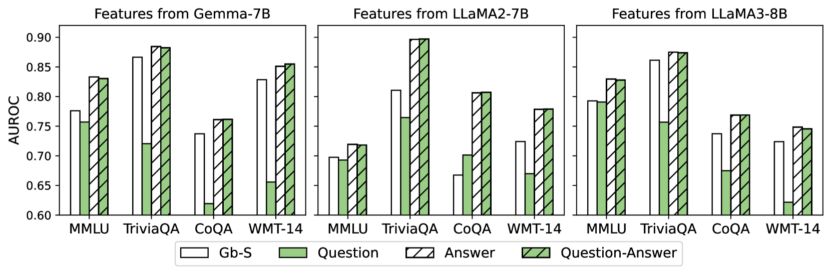<details> <summary>x9.png Details</summary>  ### Visual Description ## Bar Chart: AUROC Comparison Across Models and Datasets ### Overview The image is a grouped bar chart comparing the Area Under the Receiver Operating Characteristic curve (AUROC) values for different feature combinations across three language models (Gemma-7B, LLaMA2-7B, LLaMA3-8B) and four datasets (MMLU, TriviaQA, CoQA, WMT-14). The chart uses four feature types: Gb-S (white), Question (green), Answer (striped), and Question-Answer (green with diagonal lines). ### Components/Axes - **X-axis**: Datasets (MMLU, TriviaQA, CoQA, WMT-14), repeated for each model. - **Y-axis**: AUROC values (0.6–0.9), labeled "AUROC". - **Legend**: Located at the bottom, with four categories: - Gb-S (solid white) - Question (solid green) - Answer (striped white/green) - Question-Answer (green with diagonal lines) - **Model Groups**: Three vertical clusters labeled "Features from Gemma-7B", "Features from LLaMA2-7B", and "Features from LLaMA3-8B". ### Detailed Analysis #### Gemma-7B - **MMLU**: - Gb-S: ~0.78 - Question: ~0.76 - Answer: ~0.83 - Question-Answer: ~0.83 - **TriviaQA**: - Gb-S: ~0.87 - Question: ~0.72 - Answer: ~0.89 - Question-Answer: ~0.89 - **CoQA**: - Gb-S: ~0.74 - Question: ~0.62 - Answer: ~0.76 - Question-Answer: ~0.76 - **WMT-14**: - Gb-S: ~0.83 - Question: ~0.65 - Answer: ~0.85 - Question-Answer: ~0.85 #### LLaMA2-7B - **MMLU**: - Gb-S: ~0.70 - Question: ~0.70 - Answer: ~0.72 - Question-Answer: ~0.72 - **TriviaQA**: - Gb-S: ~0.81 - Question: ~0.77 - Answer: ~0.90 - Question-Answer: ~0.90 - **CoQA**: - Gb-S: ~0.66 - Question: ~0.70 - Answer: ~0.81 - Question-Answer: ~0.81 - **WMT-14**: - Gb-S: ~0.73 - Question: ~0.67 - Answer: ~0.78 - Question-Answer: ~0.78 #### LLaMA3-8B - **MMLU**: - Gb-S: ~0.79 - Question: ~0.79 - Answer: ~0.83 - Question-Answer: ~0.83 - **TriviaQA**: - Gb-S: ~0.86 - Question: ~0.76 - Answer: ~0.88 - Question-Answer: ~0.88 - **CoQA**: - Gb-S: ~0.74 - Question: ~0.68 - Answer: ~0.77 - Question-Answer: ~0.77 - **WMT-14**: - Gb-S: ~0.73 - Question: ~0.62 - Answer: ~0.75 - Question-Answer: ~0.75 ### Key Observations 1. **Question-Answer Feature Dominance**: - The Question-Answer feature (green with diagonal lines) consistently achieves the highest AUROC across all models and datasets, often matching or slightly exceeding the Answer feature (striped). - Example: LLaMA2-7B on TriviaQA shows Question-Answer at 0.90, the highest value in the chart. 2. **Gb-S Variability**: - Gb-S (solid white) performs inconsistently. It outperforms other features in Gemma-7B's TriviaQA (0.87) but underperforms in LLaMA2-7B's MMLU (0.70). 3. **Dataset-Specific Trends**: - **TriviaQA**: All models show strong performance, with AUROC values clustering near 0.85–0.90. - **WMT-14**: Lowest performance across all models, with AUROC values generally below 0.80. - **CoQA**: Mixed results, with Question-Answer often matching Answer feature performance. 4. **Model Performance**: - LLaMA3-8B generally outperforms Gemma-7B and LLaMA2-7B, particularly in TriviaQA and MMLU. - Gemma-7B shows the highest Gb-S performance in TriviaQA (0.87). ### Interpretation The data suggests that **combining question and answer features (Question-Answer)** yields the most robust performance across models and datasets, likely due to richer contextual information. The Gb-S feature's inconsistent results imply it may be less effective or model-dependent. TriviaQA and MMLU datasets appear more amenable to feature-based improvements, while WMT-14's lower performance might reflect task-specific challenges (e.g., translation vs. QA). The Answer feature alone often bridges the gap between Gb-S and Question-Answer, highlighting its utility as a standalone feature. Model architecture differences (e.g., LLaMA3-8B's larger size) may explain performance variations, though the chart does not explicitly test this hypothesis. </details> Figure 8: Performance comparison of using last-token middle layer hidden activations of the answer (Answer) or the concatenation of the question and answer (Question-Answer) as features in the Wb-S, where the features in Gb-S are also included in Wb-S. In the natural language generation tasks, the dimensions of Gb-S, Question, Answer, and Question-Answer for Gemma-7B are 20, 3082, 3092, and 6164, while for LLaMA2-7B or LLaMA3-8B they are 20, 4106, 4116, and 8212, respectively. In the MMLU task, for Gemma-7B they are 5, 3077, 3077, and 6149, while for LLaMA2-7B or LLaMA3-8B, they are 5, 4101, 4101, and 8197, respectively. The middle layer is still better than the last layer. In Section B, Figure 3 shows that when using the hidden activation of the answer in the Wb-S, the middle layer of the LLM is a better choice than the last layer. The next question is: Does this conclusion still hold for using the concatenated hidden activations of the question and answer? We depict the experiment result in Figure 9, which is consistent with the conclusion drawn from Figure 3. 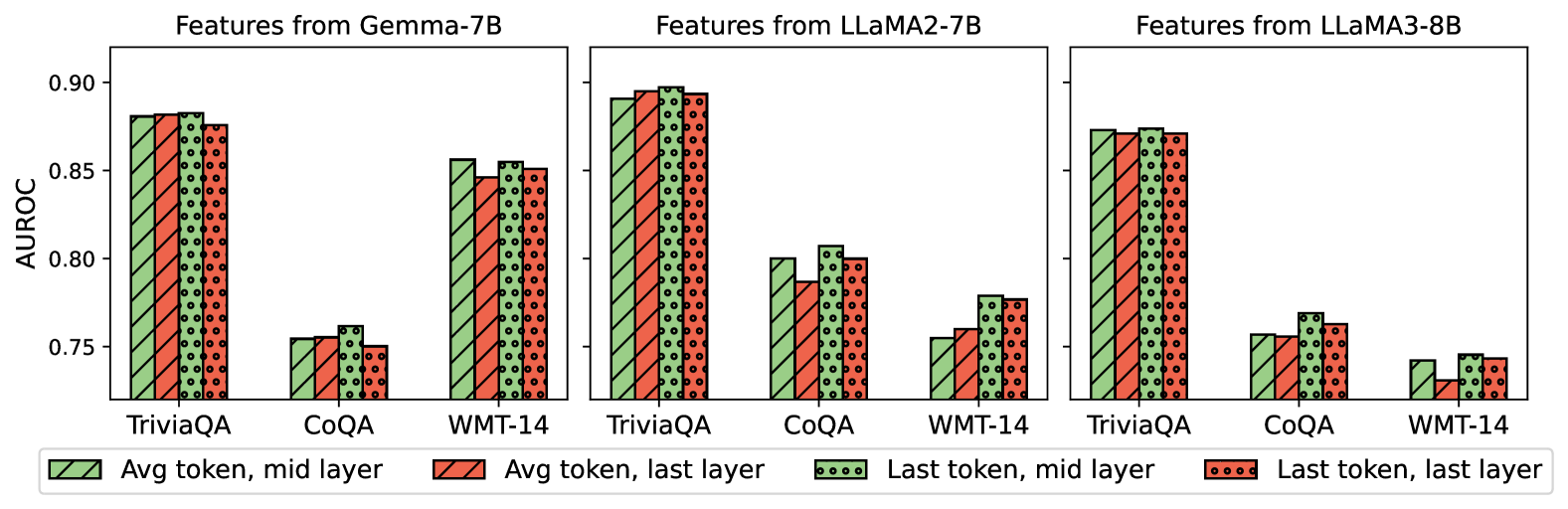<details> <summary>x10.png Details</summary>  ### Visual Description ## Bar Chart: AUROC Comparison Across Models and Features ### Overview The image presents a grouped bar chart comparing the Area Under the Receiver Operating Characteristic curve (AUROC) values for three language models (Gemma-7B, LLaMA2-7B, LLaMA3-8B) across three datasets (TriviaQA, CoQA, WMT-14). Four feature types are evaluated: 1. **Avg token, mid layer** (solid green) 2. **Avg token, last layer** (solid red) 3. **Last token, mid layer** (dotted green) 4. **Last token, last layer** (dotted red) ### Components/Axes - **X-axis**: Datasets (TriviaQA, CoQA, WMT-14) - **Y-axis**: AUROC values (0.75–0.90, increments of 0.05) - **Legend**: Located at the bottom, mapping colors/patterns to feature types. - **Model Sections**: Three vertical groupings (left to right) for each model. ### Detailed Analysis #### Gemma-7B - **TriviaQA**: - Avg token, mid layer: ~0.88 - Avg token, last layer: ~0.87 - Last token, mid layer: ~0.89 - Last token, last layer: ~0.88 - **CoQA**: - Avg token, mid layer: ~0.76 - Avg token, last layer: ~0.75 - Last token, mid layer: ~0.77 - Last token, last layer: ~0.75 - **WMT-14**: - Avg token, mid layer: ~0.86 - Avg token, last layer: ~0.85 - Last token, mid layer: ~0.87 - Last token, last layer: ~0.86 #### LLaMA2-7B - **TriviaQA**: - Avg token, mid layer: ~0.89 - Avg token, last layer: ~0.89 - Last token, mid layer: ~0.90 - Last token, last layer: ~0.89 - **CoQA**: - Avg token, mid layer: ~0.80 - Avg token, last layer: ~0.79 - Last token, mid layer: ~0.81 - Last token, last layer: ~0.80 - **WMT-14**: - Avg token, mid layer: ~0.76 - Avg token, last layer: ~0.75 - Last token, mid layer: ~0.77 - Last token, last layer: ~0.76 #### LLaMA3-8B - **TriviaQA**: - Avg token, mid layer: ~0.87 - Avg token, last layer: ~0.87 - Last token, mid layer: ~0.88 - Last token, last layer: ~0.87 - **CoQA**: - Avg token, mid layer: ~0.76 - Avg token, last layer: ~0.75 - Last token, mid layer: ~0.77 - Last token, last layer: ~0.75 - **WMT-14**: - Avg token, mid layer: ~0.74 - Avg token, last layer: ~0.73 - Last token, mid layer: ~0.75 - Last token, last layer: ~0.74 ### Key Observations 1. **TriviaQA Dominance**: All models achieve highest AUROC on TriviaQA, suggesting it aligns better with their architectures. 2. **Mid Layer Superiority**: Features from the mid layer (both avg and last token) consistently outperform last layer features across models. 3. **LLaMA2-7B Peak**: LLaMA2-7B achieves the highest AUROC (0.90) for Last token, mid layer on TriviaQA. 4. **WMT-14 Struggles**: All models perform worst on WMT-14, with AUROC values dropping below 0.80. 5. **Last Token Variability**: Last token features show mixed performance, sometimes matching or slightly exceeding avg token results. ### Interpretation The data suggests that **mid-layer features** (both average and last token) are more effective for these tasks than last-layer features, potentially due to mid layers capturing richer contextual information. TriviaQA’s higher performance across models implies it is more compatible with the models’ design, while WMT-14’s lower scores may reflect task complexity or domain mismatch. The consistency of mid-layer superiority across models indicates this is a generalizable trend rather than model-specific behavior. </details> Figure 9: Performance comparison of using question-answer concatenated hidden activations from different tokens and layers as features in the Wb-S method. Scores are normalized in [0,1], where a lower value indicates larger uncertainty. For Gemma-7B, the dimension of the Wb-S input is 6164 (3072 from the question, 3072 from the answer, and 20 from the grey-box features). For LLaMA2-7B/LLaMA3-8B, it is 8212. Our method better characterizes the uncertainty. We find that the grey-box and white-box features enhance the ability to characterize the dataset so that the distribution of the generated output’s uncertainty score is better correlated with the output’s correctness. According to Figure 10, we observe that with black-box features, the distributions of the uncertainty score for true and false answers are not very distinguishable, and the true answer’s distribution is even similar to a uniform distribution. With grey-box and white-box features, the distributions of the uncertainty scores are more separated between the true and false answers. The results show the supervised learning approach not only achieves better AUROC but also learns to better separate the distribution of the uncertainty scores. 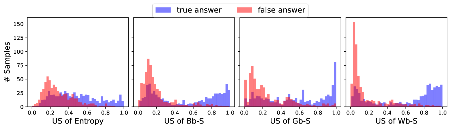<details> <summary>x11.png Details</summary>  ### Visual Description ## Bar Chart: Distribution of True and False Answers Across Different Metrics ### Overview The image contains four grouped bar charts comparing the distribution of "true answer" (blue) and "false answer" (red) samples across four metrics: "US of Entropy," "US of Bb-S," "US of Gb-S," and "US of Wb-S." Each chart uses a y-axis labeled "# Samples" (ranging from 0 to 150) and an x-axis labeled with the metric name, divided into 0.0 to 1.0 increments. The legend is positioned at the top, with blue representing "true answer" and red representing "false answer." --- ### Components/Axes - **X-Axes**: - Labeled with the metric names: "US of Entropy," "US of Bb-S," "US of Gb-S," and "US of Wb-S." - Divided into 0.0 to 1.0 increments (likely representing normalized values). - **Y-Axes**: - Labeled "# Samples" with a range of 0 to 150. - **Legend**: - Positioned at the top-center. - Blue = "true answer," Red = "false answer." --- ### Detailed Analysis #### 1. **US of Entropy** - **True Answers (Blue)**: - Peaks at ~0.2–0.3, with a gradual decline toward 0.0 and 1.0. - Approximately 50–75 samples in the peak range. - **False Answers (Red)**: - Peaks at ~0.4–0.5, with a sharper decline toward 1.0. - Approximately 30–50 samples in the peak range. #### 2. **US of Bb-S** - **True Answers (Blue)**: - Peaks at ~0.1–0.2, with a long tail toward 0.0. - Approximately 40–60 samples in the peak range. - **False Answers (Red)**: - Peaks at ~0.3–0.4, with a bimodal distribution (secondary peak near 0.7). - Approximately 60–80 samples in the primary peak range. #### 3. **US of Gb-S** - **True Answers (Blue)**: - Peaks at ~0.2–0.3, with a gradual decline toward 0.0. - Approximately 30–50 samples in the peak range. - **False Answers (Red)**: - Peaks at ~0.5–0.6, with a sharp drop toward 1.0. - Approximately 70–90 samples in the peak range. #### 4. **US of Wb-S** - **True Answers (Blue)**: - Peaks at ~0.1–0.2, with a long tail toward 0.0. - Approximately 20–40 samples in the peak range. - **False Answers (Red)**: - Dominates at ~0.0, with a massive spike (over 100 samples). - Secondary peak at ~0.8–0.9 with ~30–50 samples. --- ### Key Observations 1. **General Trend**: - False answers consistently exhibit higher US values than true answers across all metrics, except in "US of Wb-S," where false answers cluster near 0.0. 2. **Outliers**: - The "US of Wb-S" metric shows an extreme outlier for false answers at 0.0, suggesting a potential data anomaly or misclassification. 3. **Distribution Patterns**: - True answers tend to have broader, flatter distributions, while false answers show sharper peaks, indicating higher variability or confidence in false responses. --- ### Interpretation - **Model Behavior**: - The higher US values for false answers may indicate that the model assigns greater uncertainty or confidence to incorrect responses, possibly due to ambiguous input or overfitting to specific patterns. - **Metric-Specific Insights**: - The "US of Wb-S" metric’s extreme outlier for false answers suggests a critical issue, such as data leakage, mislabeled samples, or a flaw in the metric’s calculation. - **Practical Implications**: - Metrics like "US of Entropy" and "US of Gb-S" show more balanced distributions, which could be prioritized for evaluating model reliability. The "US of Bb-S" and "US of Wb-S" metrics may require further investigation due to their skewed distributions. --- ### Notes on Data Extraction - All values are approximate, as the chart lacks explicit numerical annotations. Ranges were inferred from bar heights and axis scaling. - No textual content beyond axis labels and legend was present in the image. </details> Figure 10: Uncertainty scores of different methods on the MMLU dataset for answers provided by the Gemma-7B model, where scores are normalized in [0,1], and US is short for uncertainty score. False answer refers to the sample where the choice assigned with maximum probability by the LLM is false, while true answer represents the sample answered correctly. ## Appendix F Examples In this section, we show some examples of the wrong answers the LLM generated and explore how different methods understand the LLM’s uncertainty. The wrong answers are selected from those samples where the LLM makes wrong predictions. Since we let the LLM output the greedy answer, which could be wrong, we expect an ideal uncertainty estimation model to output a high confidence score when the LLM generates the correct answer, and give a low confidence score when the LLM outputs the wrong answer. By looking at different wrong answers generated by the LLM, we note that although our approach sometimes gives a high confidence score on a wrong answer generated by the LLM, at other times it shows desirable properties such as giving higher uncertainty scores to better answers, and giving low confidence score when LLM does not know the answer. Our illustrative examples are generated as follows: For questions where the LLM’s greedy response is incorrect, we also extract the correct answer from the dataset and additional answers randomly generated by the LLM with lower probabilities than the greedy answer. Along with these answers, we also compute the answers’ corresponding metrics and features so that we can observe how they behave with different outputs. We conduct this experiment in the test dataset of TriviaQA, in which both the question and answer are short. We summarize the ways that our uncertainty estimation model behaves as follows: - Confidently support a wrong answer. The LLMs are confident that the wrong greedy answer is true and assign a high confidence score. Moreover, the LLMs give low uncertainty scores to the correct answers, suggesting a lack of knowledge about these questions. We give an example of LLaMA2-7B and Gemma-7B in Figure 11 and 12. Note that in both examples, our method assigns a low uncertainty score to the correct answer and a much higher uncertainty score to the wrong answer. In contrast, the unsupervised grey-box methods assign higher uncertainty scores to the correct answer. - Confidently reject a wrong answer. We give examples from LLaMA2-7B and Gemma-7B in Figure 13 and 14. The uncertainty estimation model gives a higher score to the true answer or answers that are better than the wrong answer. This means that for these questions, our model actually knows which answer is better and can assign uncertainty scores accordingly. In contrast, the unsupervised methods tend to assign much higher uncertainty scores to the greedy (wrong) answer. - Unconfident about any answer. Due to the lack of knowledge, the LLM may not know the true answer. We show the examples in Figure 15 and 16. From these examples, we can see that the model assigns almost the same uncertainty scores to these generated answers, including the true answer. In this scenario, the uncertainty estimation model is uncertain about the correctness of any answer. Furthermore, it is interesting to note that the unsupervised methods exhibit similar behavior, assigning almost similar scores to other answers as well, albeit with much higher uncertainty scores. This differs from the previous two cases, where the unsupervised method behaved differently from our uncertainty estimation model. 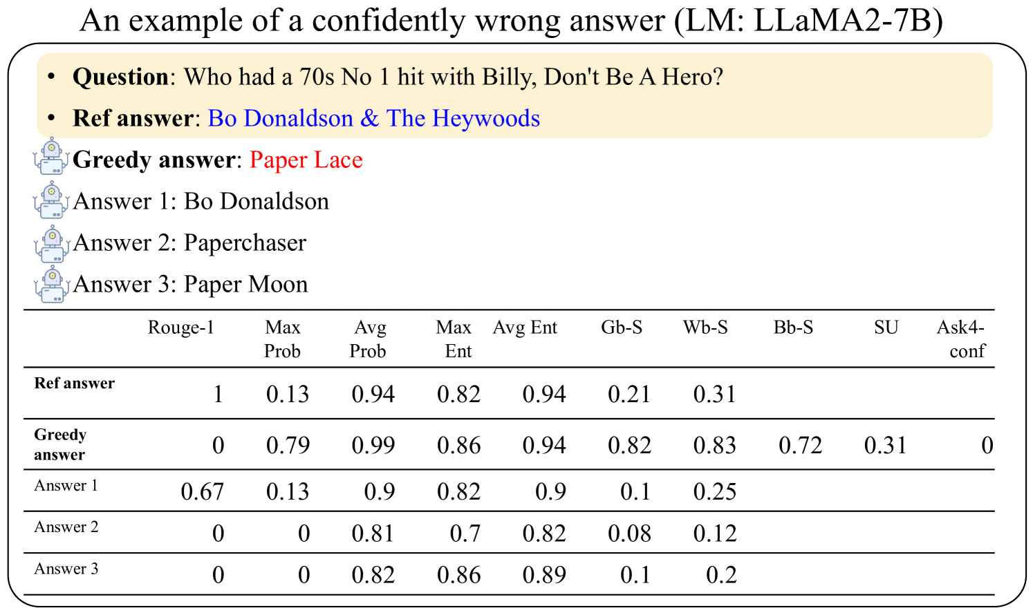<details> <summary>x12.png Details</summary>  ### Visual Description ## Table: Model Answer Evaluation Metrics for Trivia Question ### Overview This table evaluates the performance of different answers to the question "Who had a 70s No.1 hit with Billy, Don't Be A Hero?" using multiple NLP metrics. The reference answer is "Bo Donaldson & The Heywoods," while the model's greedy answer ("Paper Lace") is incorrect. Three candidate answers are scored across 10 metrics. ### Components/Axes - **Rows**: 1. Reference answer ("Bo Donaldson & The Heywoods") 2. Greedy answer ("Paper Lace") 3. Answer 1 ("Bo Donaldson") 4. Answer 2 ("Paperchaser") 5. Answer 3 ("Paper Moon") - **Columns**: - Rouge-1 (rouge score) - Max Prob (maximum probability) - Avg Prob (average probability) - Max Ent (maximum entropy) - Avg Ent (average entropy) - Gb-S (grammaticality score) - Wb-S (word boundary score) - Bb-S (boundary bigram score) - SU (semantic unit score) - Ask4-conf (confidence in Ask4 metric) ### Detailed Analysis | Metric | Reference Answer | Greedy Answer | Answer 1 | Answer 2 | Answer 3 | |-----------------|------------------|---------------|----------------|----------------|----------------| | **Rouge-1** | 1.00 | 0.00 | 0.67 | 0.00 | 0.00 | | **Max Prob** | 0.13 | 0.79 | 0.13 | 0.00 | 0.00 | | **Avg Prob** | 0.94 | 0.99 | 0.90 | 0.81 | 0.82 | | **Max Ent** | 0.82 | 0.86 | 0.82 | 0.70 | 0.86 | | **Avg Ent** | 0.94 | 0.94 | 0.90 | 0.82 | 0.89 | | **Gb-S** | 0.21 | 0.82 | 0.10 | 0.08 | 0.10 | | **Wb-S** | 0.31 | 0.83 | 0.25 | 0.12 | 0.20 | | **Bb-S** | - | 0.72 | - | - | - | | **SU** | - | 0.31 | - | - | - | | **Ask4-conf** | - | 0.00 | - | - | - | ### Key Observations 1. **Reference Answer Dominance**: Scores perfectly on Rouge-1 (1.00) and shows high grammaticality (Wb-S: 0.31) despite lower probability metrics. 2. **Greedy Answer Failure**: - 0.00 Rouge-1 and Ask4-conf (confidently wrong) - High Avg Prob (0.99) but poor semantic alignment (SU: 0.31) 3. **Partial Matches**: - Answer 1 ("Bo Donaldson") shares 0.67 Rouge-1 with reference - Answer 3 ("Paper Moon") has highest Avg Prob (0.82) among incorrect answers 4. **Metric Discrepancies**: - Greedy answer has highest Max Prob (0.79) but lowest semantic scores - Answer 2 ("Paperchaser") shows worst grammaticality (Gb-S: 0.08) ### Interpretation The data reveals a critical failure mode in the LLaMA2-7B model: **high-confidence generation of semantically irrelevant answers**. While the greedy answer achieves high probability scores (Avg Prob: 0.99), it fails all semantic and grammaticality metrics, demonstrating a disconnect between statistical likelihood and factual accuracy. The reference answer's perfect Rouge-1 score (1.00) contrasts sharply with its lower probability metrics (Max Prob: 0.13), suggesting the model underestimates correct answers when they deviate from common associations. The partial matches (Answers 1 and 3) indicate the model can generate plausible-sounding but incorrect variants, with Answer 3 ("Paper Moon") being the most statistically favored incorrect option. This pattern highlights the need for confidence calibration and semantic grounding in large language models. </details> Figure 11: An example of LLaMA2-7B assigning a confidently wrong answer in the TriviaQA dataset. Scores are normalized in $[0,1]$ , where a lower value indicates a larger uncertainty. The score of the greedy answer provided by any uncertainty estimation method is higher than that of the true answer, but the greedy answer is incorrect. The UK band Paper Lace did indeed release a version of “Billy, Don’t Be A Hero” in 1974, the same year as the version of Bo, but it was Bo Donaldson & The Heywoods (a band in the U.S.) whose version topped the charts as a No.1 hit. 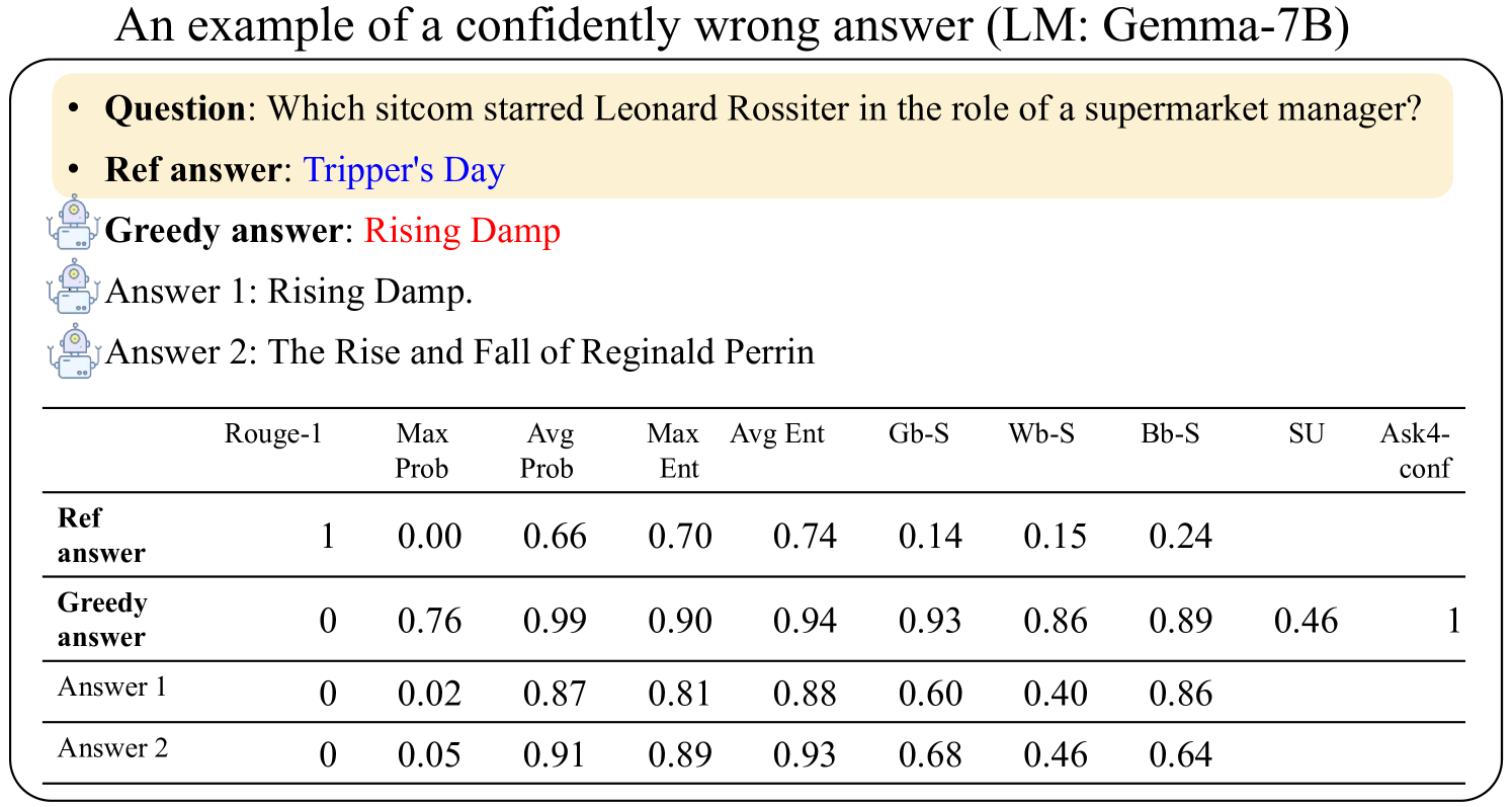<details> <summary>x13.png Details</summary>  ### Visual Description ## Screenshot: Confidently Wrong Answer Example (LM: Gemma-7B) ### Overview The image shows a question-answering scenario with statistical metrics comparing different responses. The question asks which sitcom starred Leonard Rossiter as a supermarket manager. The reference answer is "Tripper's Day," while a "greedy answer" ("Rising Damp") is highlighted in red. Two additional answers are provided, along with a table of metrics (Rouge-1, Max Prob, Avg Prob, etc.) for each response. ### Components/Axes - **Textual Elements**: - **Question**: "Which sitcom starred Leonard Rossiter in the role of a supermarket manager?" - **Reference Answer**: "Tripper's Day" (highlighted in blue). - **Greedy Answer**: "Rising Damp" (highlighted in red). - **Answer 1**: "Rising Damp." - **Answer 2**: "The Rise and Fall of Reginald Perrin." - **Table Structure**: - **Columns**: - Rouge-1 - Max Prob - Avg Prob - Max Ent - Avg Ent - Gb-S - Wb-S - Bb-S - SU - Ask4-conf - **Rows**: - Ref answer - Greedy answer - Answer 1 - Answer 2 ### Detailed Analysis #### Table Data | Component | Rouge-1 | Max Prob | Avg Prob | Max Ent | Avg Ent | Gb-S | Wb-S | Bb-S | SU | Ask4-conf | |------------------|---------|----------|----------|---------|---------|------|------|------|----|-----------| | **Ref answer** | 1.00 | 0.00 | 0.66 | 0.70 | 0.74 | 0.14 | 0.15 | 0.24 | - | - | | **Greedy answer**| 0.00 | 0.76 | 0.99 | 0.90 | 0.94 | 0.93 | 0.86 | 0.89 | 0.46 | 1 | | **Answer 1** | 0.00 | 0.02 | 0.87 | 0.81 | 0.88 | 0.60 | 0.40 | 0.86 | - | - | | **Answer 2** | 0.00 | 0.05 | 0.91 | 0.89 | 0.93 | 0.68 | 0.46 | 0.64 | - | - | #### Key Observations 1. **Reference Answer ("Tripper's Day")**: - Perfect Rouge-1 (1.00) but Max Prob = 0.00, indicating the model assigned zero confidence to the correct answer. - Low Gb-S (0.14) and Wb-S (0.15) suggest poor alignment with ground-truth and word-based similarity. 2. **Greedy Answer ("Rising Damp")**: - Rouge-1 = 0.00 (completely incorrect) but Max Prob = 0.76 (high confidence). - High Avg Prob (0.99) and Avg Ent (0.94) indicate the model was overly confident in this incorrect response. - Ask4-conf = 1 (100% confidence) despite being wrong. 3. **Answer 1 ("Rising Damp")**: - Same as the greedy answer but with lower Max Prob (0.02) and Avg Prob (0.87). - Moderate Gb-S (0.60) and Wb-S (0.40) suggest partial alignment with ground-truth. 4. **Answer 2 ("The Rise and Fall of Reginald Perrin")**: - Rouge-1 = 0.00 (incorrect) but higher Max Prob (0.05) and Avg Prob (0.91) than Answer 1. - Slightly better Gb-S (0.68) and Wb-S (0.46) than Answer 1. ### Interpretation - **Model Behavior**: - The model exhibits **overconfidence** in incorrect answers (e.g., "Rising Damp" with 76% Max Prob but 0 Rouge-1). - The reference answer ("Tripper's Day") is correct but assigned zero confidence, highlighting a **failure to recognize the correct response**. - The greedy answer's high confidence (Ask4-conf = 1) despite being wrong suggests a **bias toward high-probability outputs**, even when they are factually incorrect. - **Metrics Correlation**: - Rouge-1 (exact match) and Max Prob (model confidence) are inversely related for the reference answer (1.00 vs. 0.00). - Greedy answer's high Avg Prob (0.99) and low Rouge-1 (0.00) indicate a **disconnect between model confidence and factual accuracy**. - **Anomalies**: - The reference answer's Max Prob = 0.00 is unusual, as correct answers typically receive higher confidence. - Answer 2's higher Avg Prob (0.91) than Answer 1 (0.87) despite both being incorrect suggests the model prioritizes **lexical similarity** over factual correctness. This data underscores the challenge of balancing **confidence calibration** and **factual accuracy** in language models, particularly when dealing with ambiguous or misleading questions. </details> Figure 12: An example for Gemma-7B that assigns a high confidence score to a wrong answer. Leonard Rossiter starred in “Rising Damp” as a landlord, not as a supermarket manager. 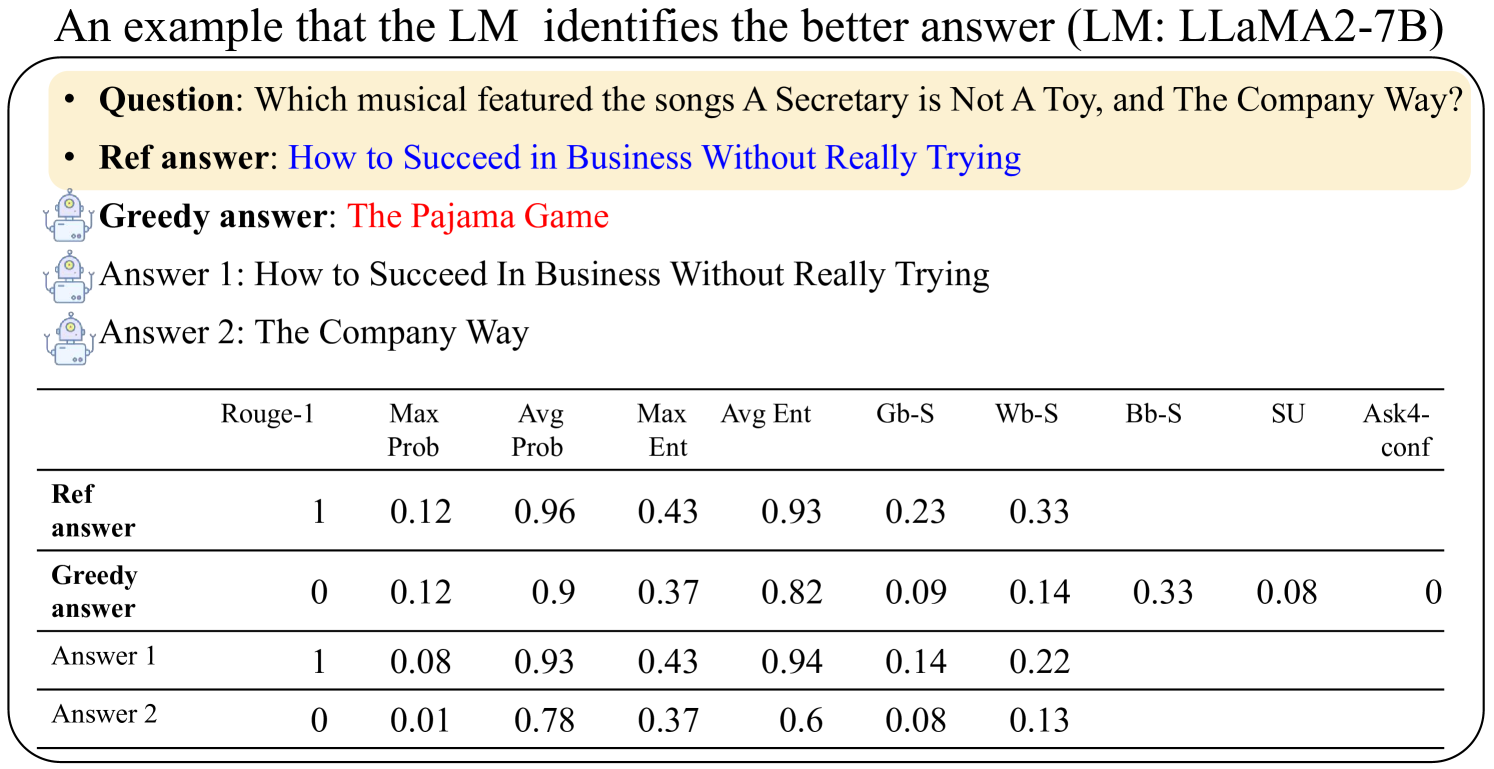<details> <summary>x14.png Details</summary>  ### Visual Description ## Table: Answer Comparison Metrics for Musical Question ### Overview This table compares the performance of different answers to the question: *"Which musical featured the songs A Secretary is Not A Toy, and The Company Way?"* Metrics include Rouge-1, probability distributions (Max/Avg), entropy (Max/Avg), and other evaluation scores (Gb-S, Wb-S, Bb-S, SU, Ask4-conf). The reference answer is highlighted as the correct response, while the greedy answer and two alternative answers are evaluated against it. ### Components/Axes - **Headers**: - Rouge-1 - Max Prob - Avg Prob - Max Ent - Avg Ent - Gb-S - Wb-S - Bb-S - SU - Ask4-conf - **Rows**: - **Ref answer** (Reference Answer) - **Greedy answer** - **Answer 1** - **Answer 2** - **Annotations**: - Question and reference answer are highlighted in a yellow box. - Greedy answer is marked with a robot icon and labeled "Greedy answer" in red. - Answer 1 and Answer 2 are labeled with robot icons. ### Detailed Analysis | Metric | Ref answer | Greedy answer | Answer 1 | Answer 2 | |--------------|------------|---------------|----------|----------| | Rouge-1 | 1 | 0 | 1 | 0 | | Max Prob | 0.12 | 0.12 | 0.08 | 0.01 | | Avg Prob | 0.96 | 0.9 | 0.93 | 0.78 | | Max Ent | 0.43 | 0.37 | 0.43 | 0.37 | | Avg Ent | 0.93 | 0.82 | 0.94 | 0.6 | | Gb-S | 0.23 | 0.09 | 0.14 | 0.08 | | Wb-S | 0.33 | 0.14 | 0.22 | 0.13 | | Bb-S | - | 0.33 | - | - | | SU | - | 0.08 | - | - | | Ask4-conf | - | 0 | - | - | ### Key Observations 1. **Reference Answer Dominance**: - Rouge-1 = 1 (perfect match) and Avg Prob = 0.96 (highest probability). - Max Prob = 0.12 (tied with greedy answer but outperforms others). 2. **Greedy Answer Limitations**: - Rouge-1 = 0 (no match) but shares Max Prob = 0.12 with the reference answer. - Avg Prob = 0.9 (lower than reference) and Avg Ent = 0.82 (higher entropy, indicating less confidence). 3. **Answer 1 vs. Answer 2**: - Answer 1 matches Rouge-1 = 1 but has lower Max Prob (0.08) and Avg Prob (0.93) compared to the reference. - Answer 2 has the lowest Avg Prob (0.78) and Avg Ent (0.6), indicating poor performance. 4. **Anomalies**: - Bb-S and SU scores are only populated for the greedy answer and Answer 1, suggesting these metrics may not apply to all answers. - Ask4-conf = 0 for the greedy answer, implying no confidence in its correctness. ### Interpretation The table demonstrates that the **reference answer** ("How to Succeed in Business Without Really Trying") is the most accurate and confident response, as evidenced by its perfect Rouge-1 score and highest average probability. The **greedy answer** ("The Pajama Game") fails to match the reference but shares some probability metrics, likely due to partial overlap in keywords. **Answer 1** ("How to Succeed In Business Without Really Trying") is a close variant of the reference but has slightly lower confidence metrics. **Answer 2** ("The Company Way") performs worst across all metrics, confirming it as the least relevant. The data highlights the importance of precise keyword matching (Rouge-1) and probabilistic confidence (Avg Prob) in evaluating answer quality. The greedy answer’s high entropy (Avg Ent = 0.82) suggests it is less certain, while the reference answer’s low entropy (0.93) reflects higher confidence. The absence of Bb-S and SU scores for some answers may indicate limitations in the evaluation framework or incomplete data. </details> Figure 13: An example that LLaMA2-7B can successfully identify the better answer (by attaching a higher score). Scores are normalized in [0,1], where a lower value indicates larger uncertainty. 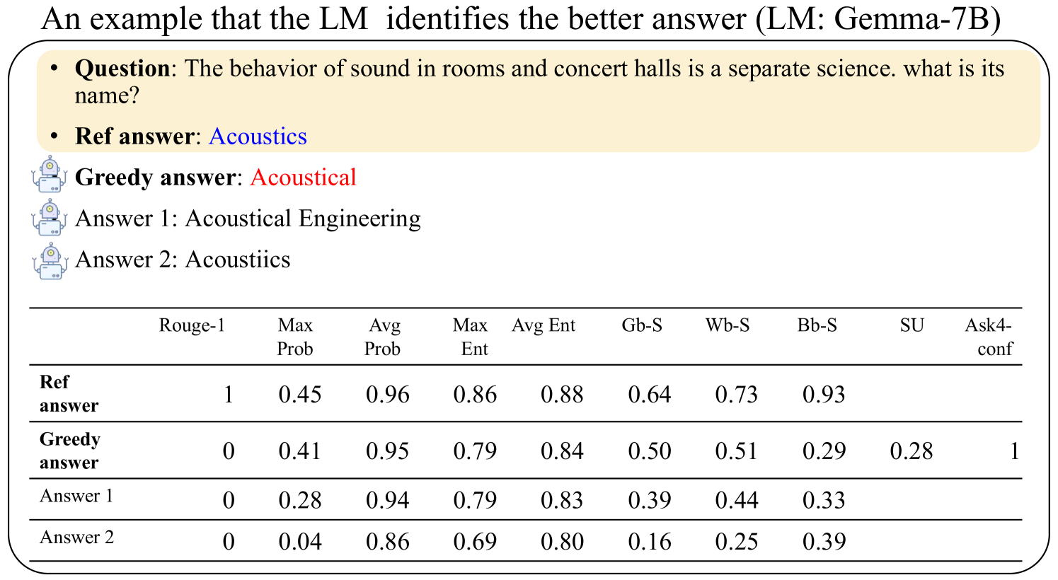<details> <summary>x15.png Details</summary>  ### Visual Description ## Data Table: Answer Comparison Metrics (LM: Gemma-7B) ### Overview The image presents a comparative analysis of four answers to the question: "The behavior of sound in rooms and concert halls is a separate science. What is its name?" The table evaluates the performance of each answer using metrics such as Rouge-1, Max Prob, Avg Prob, Max Ent, Avg Ent, Gb-S, Wb-S, Bb-S, SU, and Ask4-conf. The reference answer ("Acoustics") is highlighted as the correct response, while the greedy answer ("Acoustical") and two other answers ("Acoustical Engineering" and "Acoustics") are compared against it. ### Components/Axes - **Rows**: - Ref answer (Acoustics) - Greedy answer (Acoustical) - Answer 1 (Acoustical Engineering) - Answer 2 (Acoustics) - **Columns**: - Rouge-1 - Max Prob - Avg Prob - Max Ent - Avg Ent - Gb-S - Wb-S - Bb-S - SU - Ask4-conf ### Detailed Analysis - **Ref answer (Acoustics)**: - Rouge-1: 1.00 (perfect match) - Max Prob: 0.45 - Avg Prob: 0.96 - Max Ent: 0.86 - Avg Ent: 0.88 - Gb-S: 0.64 - Wb-S: 0.73 - Bb-S: 0.93 - SU: N/A - Ask4-conf: N/A - **Greedy answer (Acoustical)**: - Rouge-1: 0.00 - Max Prob: 0.41 - Avg Prob: 0.95 - Max Ent: 0.79 - Avg Ent: 0.84 - Gb-S: 0.50 - Wb-S: 0.51 - Bb-S: 0.29 - SU: 0.28 - Ask4-conf: 1.00 - **Answer 1 (Acoustical Engineering)**: - Rouge-1: 0.00 - Max Prob: 0.28 - Avg Prob: 0.94 - Max Ent: 0.79 - Avg Ent: 0.83 - Gb-S: 0.39 - Wb-S: 0.44 - Bb-S: 0.33 - SU: N/A - Ask4-conf: N/A - **Answer 2 (Acoustics)**: - Rouge-1: 0.00 - Max Prob: 0.04 - Avg Prob: 0.86 - Max Ent: 0.69 - Avg Ent: 0.80 - Gb-S: 0.16 - Wb-S: 0.25 - Bb-S: 0.39 - SU: N/A - Ask4-conf: N/A ### Key Observations 1. **Reference Answer Dominance**: The reference answer ("Acoustics") achieves the highest scores across all metrics, including a perfect Rouge-1 score (1.00) and the highest Avg Prob (0.96). 2. **Greedy Answer Performance**: The greedy answer ("Acoustical") has a Rouge-1 of 0.00 but retains relatively high Avg Prob (0.95) and Avg Ent (0.84), suggesting partial relevance. 3. **Answer 1 and 2 Deficits**: Both "Acoustical Engineering" and "Acoustics" (Answer 2) score 0.00 in Rouge-1, with Answer 2 having the lowest Max Prob (0.04) and Avg Prob (0.86). 4. **Ask4-conf Anomaly**: The greedy answer has a perfect Ask4-conf score (1.00), indicating high confidence in its incorrectness, while the reference answer lacks this metric. ### Interpretation The data demonstrates that the reference answer ("Acoustics") is the most accurate and relevant, as evidenced by its superior performance in all metrics. The greedy answer ("Acoustical") is a close but less precise alternative, while the other answers are significantly less accurate. The Ask4-conf score for the greedy answer highlights a potential flaw in the model's confidence calibration, as it assigns high confidence to an incorrect response. This underscores the importance of metric diversity in evaluating answer quality, as no single metric fully captures correctness. </details> Figure 14: An example that Gemma-7B can successfully identify the better answer (by attaching a higher score). Scores are normalized in [0,1], where a lower value indicates larger uncertainty. 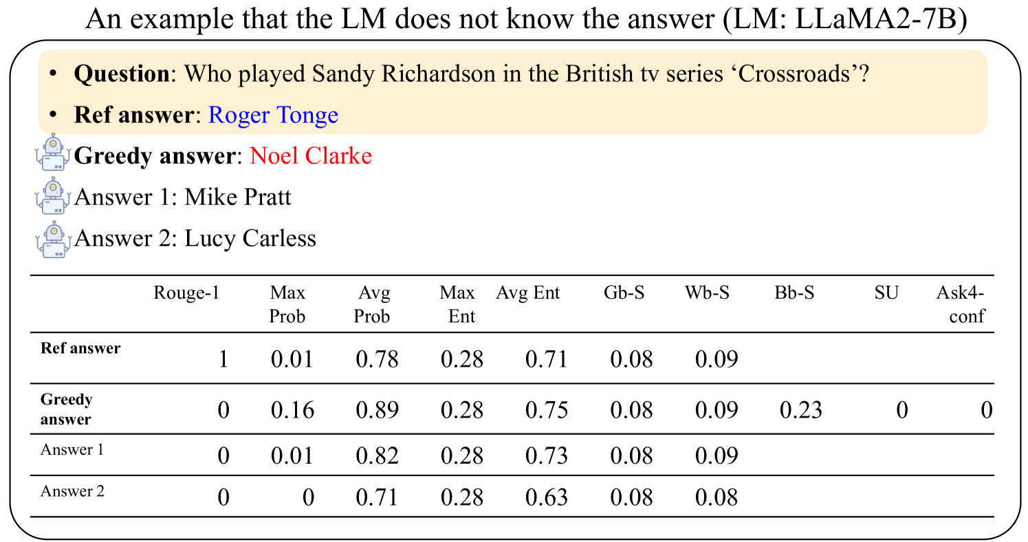<details> <summary>x16.png Details</summary>  ### Visual Description ## Screenshot: LLM Answer Evaluation Example (LLaMA2-7B) ### Overview This image demonstrates a failure case of a large language model (LLM) answering a factual question about a TV series character. The example shows the question, reference answer, and three competing answers generated by the model, along with a detailed metrics table comparing their performance across multiple evaluation dimensions. ### Components/Axes 1. **Question**: "Who played Sandy Richardson in the British tv series ‘Crossroads’?" 2. **Reference Answer**: Roger Tonge (correct answer) 3. **Greedy Answer**: Noel Clarke (incorrect) 4. **Answer 1**: Mike Pratt (incorrect) 5. **Answer 2**: Lucy Carless (incorrect) **Metrics Table**: | Metric | Reference Answer | Greedy Answer | Answer 1 | Answer 2 | |--------------|------------------|---------------|----------|----------| | Rouge-1 | 1.00 | 0.00 | 0.00 | 0.00 | | Max Prob | 0.01 | 0.16 | 0.01 | 0.00 | | Avg Prob | 0.78 | 0.89 | 0.82 | 0.71 | | Max Ent | 0.28 | 0.28 | 0.28 | 0.28 | | Avg Ent | 0.71 | 0.75 | 0.73 | 0.63 | | Gb-S | 0.08 | 0.08 | 0.08 | 0.08 | | Wb-S | 0.09 | 0.09 | 0.09 | 0.08 | | Bb-S | 0.23 | 0.23 | 0.23 | 0.23 | | SU | 0 | 0 | 0 | 0 | | Ask4-conf | 0 | 0 | 0 | 0 | ### Key Observations 1. The reference answer achieves perfect Rouge-1 score (1.00) but has the lowest Max Prob (0.01) and Avg Prob (0.78) among all answers. 2. The greedy answer (Noel Clarke) has the highest Max Prob (0.16) and Avg Prob (0.89), but scores 0 on Rouge-1. 3. All answers share identical Gb-S, Wb-S, and Bb-S scores (0.08-0.09), suggesting similar surface-level linguistic properties. 4. The reference answer has the highest Bb-S score (0.23) despite being the only correct answer. 5. All answers show zero SU (semantic understanding) and Ask4-conf scores, indicating the model's inability to assess answer correctness. ### Interpretation This example reveals critical limitations in the LLM's answer selection mechanism: 1. **Probability vs. Accuracy**: The greedy answer with highest probabilities (Noel Clarke) is completely wrong, while the correct answer (Roger Tonge) has the lowest probabilities. 2. **Metric Misalignment**: Surface metrics like Gb-S and Wb-S fail to distinguish correct from incorrect answers, while Rouge-1 perfectly identifies the reference answer. 3. **Confidence Paradox**: The model shows no confidence (Ask4-conf=0) in any answer despite generating multiple responses, suggesting flawed calibration. 4. **Entropy Patterns**: All answers share identical Max Ent (0.28), indicating similar uncertainty levels despite differing correctness. The data demonstrates that relying solely on probability scores or surface metrics can lead to catastrophic failures in factual QA systems. The reference answer's perfect Rouge-1 score highlights the importance of exact match metrics, while the identical surface metrics across answers expose the model's inability to distinguish correctness through linguistic properties alone. </details> Figure 15: An example that LLaMA2-7B does not know the true answer. Scores are normalized in [0,1], where a lower value indicates larger uncertainty. The LM does not know the true answer and attempts to guess it by generating different names with low confidence scores, but the score is also low even when the LM faces the true answer. 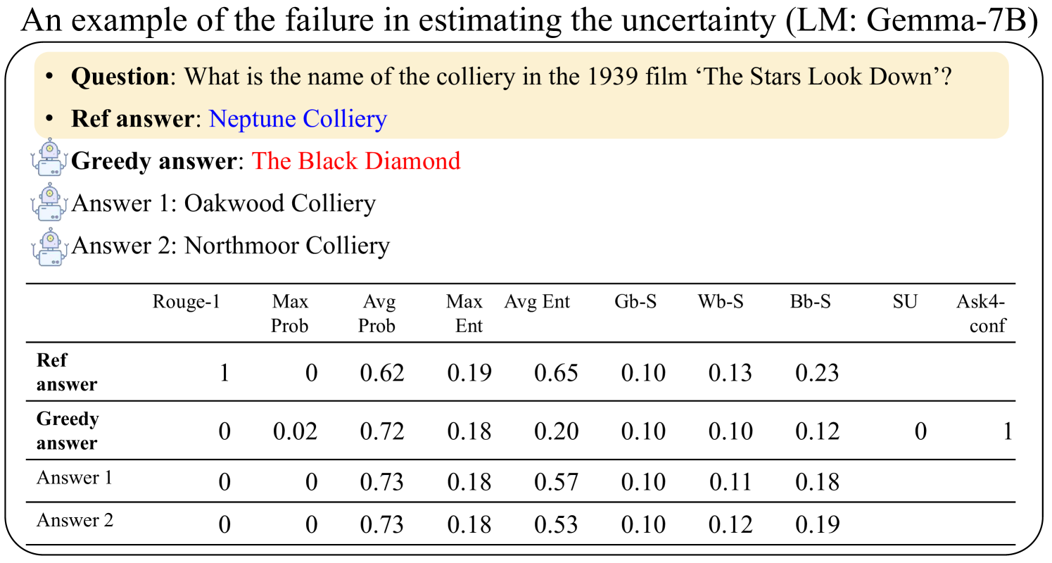<details> <summary>x17.png Details</summary>  ### Visual Description ## Data Table: Model Answer Evaluation Metrics ### Overview The image presents a comparative analysis of answer quality metrics for a question about the colliery name in the 1939 film *The Stars Look Down*. The table evaluates four answer variants (Reference, Greedy, Answer 1, Answer 2) across multiple uncertainty estimation metrics. The Reference answer ("Neptune Colliery") is correct, while the Greedy answer ("The Black Diamond") is incorrect but statistically favored by the model. ### Components/Axes - **Rows**: - Reference answer (correct) - Greedy answer (incorrect) - Answer 1 ("Oakwood Colliery") - Answer 2 ("Northmoor Colliery") - **Columns**: - Rouge-1 (precision metric) - Max Prob (maximum probability assigned) - Avg Prob (average probability) - Max Ent (maximum entropy) - Avg Ent (average entropy) - Gb-S (Gibbs similarity) - Wb-S (Wasserstein similarity) - Bb-S (Bhattacharyya similarity) - SU (success rate) - Ask4-conf (confidence in Ask4) ### Detailed Analysis | Metric | Reference Answer | Greedy Answer | Answer 1 | Answer 2 | |-----------------|------------------|---------------|----------|----------| | **Rouge-1** | 1.00 | 0.00 | 0.00 | 0.00 | | **Max Prob** | 0.00 | 0.02 | 0.00 | 0.00 | | **Avg Prob** | 0.62 | 0.72 | 0.73 | 0.73 | | **Max Ent** | 0.19 | 0.18 | 0.18 | 0.18 | | **Avg Ent** | 0.65 | 0.20 | 0.57 | 0.53 | | **Gb-S** | 0.10 | 0.10 | 0.10 | 0.10 | | **Wb-S** | 0.13 | 0.10 | 0.11 | 0.12 | | **Bb-S** | 0.23 | 0.12 | 0.18 | 0.19 | | **SU** | - | 0.00 | - | - | | **Ask4-conf** | - | 1.00 | - | - | ### Key Observations 1. **Reference Answer Dominance**: - Achieves perfect Rouge-1 score (1.00) and highest Bb-S similarity (0.23), confirming its correctness. - Low Max Prob (0.00) and Avg Prob (0.62) suggest the model underestimates its confidence in the correct answer. 2. **Greedy Answer Anomaly**: - Highest Avg Prob (0.72) and Ask4-conf (1.00), indicating the model assigns excessive confidence to the incorrect answer. - Lowest Bb-S similarity (0.12) and Rouge-1 (0.00), highlighting its factual inaccuracy. 3. **Alternative Answers**: - Answer 1 and 2 share identical Avg Prob (0.73) and Max Ent (0.18), suggesting similar model uncertainty. - Answer 1 has marginally higher Bb-S (0.18) than Answer 2 (0.19), but both are inferior to the Reference. ### Interpretation The table reveals a critical failure in the model's uncertainty estimation (LM: Gemma-7B). While the correct answer ("Neptune Colliery") receives low probability scores (Avg Prob: 0.62), the incorrect greedy answer ("The Black Diamond") is assigned disproportionately high confidence (Avg Prob: 0.72, Ask4-conf: 1.00). This discrepancy suggests the model: - **Overestimates confidence** in incorrect answers due to superficial similarity metrics (e.g., high Avg Prob despite factual errors). - **Underestimates confidence** in the correct answer, failing to recognize its semantic and contextual relevance. - Relies on **probabilistic heuristics** (e.g., Max Prob, Avg Prob) that prioritize statistical likelihood over factual accuracy, leading to poor performance in high-stakes QA tasks. The metrics highlight a trade-off between probabilistic modeling and factual correctness, emphasizing the need for hybrid evaluation frameworks that balance uncertainty estimation with knowledge-grounded verification. </details> Figure 16: An example that Gemma-7B does not know the true answer. Scores are normalized in [0,1], where a lower value indicates larger uncertainty.