2404.19737v1

# Better & Faster Large Language Models via Multi-token Prediction ## Better & Faster Large Language Models via Multi-token Prediction Fabian Gloeckle * 1 2 Badr Youbi Idrissi * 1 3 Baptiste Rozière 1 David Lopez-Paz + 1 Gabriel Synnaeve + 1 ## Abstract Large language models such as GPT and Llama are trained with a next-token prediction loss. In this work, we suggest that training language models to predict multiple future tokens at once results in higher sample efficiency. More specifically, at each position in the training corpus, we ask the model to predict the following n tokens using n independent output heads, operating on top of a shared model trunk. Considering multi-token prediction as an auxiliary training task, we measure improved downstream capabilities with no overhead in training time for both code and natural language models. The method is increasingly useful for larger model sizes, and keeps its appeal when training for multiple epochs. Gains are especially pronounced on generative benchmarks like coding, where our models consistently outperform strong baselines by several percentage points. Our 13B parameter models solves 12 % more problems on HumanEval and 17 % more on MBPP than comparable next-token models. Experiments on small algorithmic tasks demonstrate that multi-token prediction is favorable for the development of induction heads and algorithmic reasoning capabilities. As an additional benefit, models trained with 4-token prediction are up to 3 × faster at inference, even with large batch sizes. ## 1. Introduction Humanity has condensed its most ingenious undertakings, surprising findings and beautiful productions into text. Large Language Models (LLMs) trained on all of these corpora are able to extract impressive amounts of world knowledge, as well as basic reasoning capabilities by implementing a simple-yet powerful-unsupervised learning task: next-token prediction. Despite the recent wave of impressive achievements (OpenAI, 2023), next-token pre- * Equal contribution + Last authors 1 FAIR at Meta 2 CERMICS Ecole des Ponts ParisTech 3 LISN Université Paris-Saclay. Correspondence to: Fabian Gloeckle <fgloeckle@meta.com>, Badr Youbi Idrissi <byoubi@meta.com>. diction remains an inefficient way of acquiring language, world knowledge and reasoning capabilities. More precisely, teacher forcing with next-token prediction latches on local patterns and overlooks 'hard' decisions. Consequently, it remains a fact that state-of-the-art next-token predictors call for orders of magnitude more data than human children to arrive at the same level of fluency (Frank, 2023). 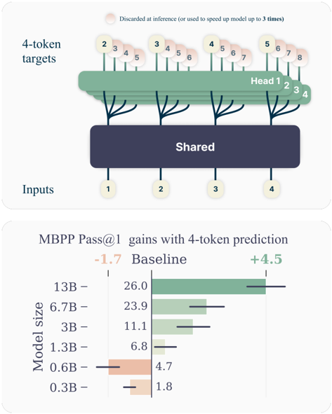Figure 1: Overview of multi-token prediction. (Top) During training, the model predicts 4 future tokens at once, by means of a shared trunk and 4 dedicated output heads. During inference, we employ only the next-token output head. Optionally, the other three heads may be used to speed-up inference time. (Bottom) Multi-token prediction improves pass@1 on the MBPP code task, significantly so as model size increases. Error bars are confidence intervals of 90% computed with bootstrapping over dataset samples. <details> <summary>Image 1 Details</summary>  ### Visual Description ## Diagram & Bar Chart: Model Performance with 4-Token Prediction ### Overview The image presents a diagram illustrating a model architecture with 4-token targets and a subsequent bar chart showing the gains in MBPP Pass@1 performance with 4-token prediction across different model sizes. The diagram depicts an input layer feeding into a shared layer, which then branches out into multiple "Heads" processing 4-token targets. The bar chart compares the performance of models of varying sizes against a baseline. ### Components/Axes **Diagram:** * **Inputs:** Labeled with numbers 1 through 4, representing the input data. * **Shared:** A dark blue rectangular block representing a shared layer in the model. * **Head 1, Head 2, Head 3, Head 4:** Green leaf-like structures representing the heads of the model. * **4-token targets:** Labeled at the top, with numbers 1 through 8 indicating the token positions. * **Discarded at inference:** A light orange bubble with text "Discarded at inference (or used to speed up model up to 3 times)". **Bar Chart:** * **Y-axis:** "Model size" with values: 0.3B, 0.6B, 1.3B, 3B, 6.7B, 13B. * **X-axis:** "MBPP Pass@1 gains with 4-token prediction" ranging from approximately -1.7 to +4.5. * **Baseline:** A vertical line at 0, indicating the baseline performance. * **Color Coding:** Green bars represent positive gains, while orange bars represent negative gains. ### Detailed Analysis or Content Details **Diagram:** The diagram shows a model architecture where inputs (1-4) are processed through a "Shared" layer. This shared layer then feeds into four separate "Heads". Each head processes a sequence of 4 tokens (indicated by the "4-token targets" label and the numbers 1-8 above the heads). The orange bubble indicates that some information is discarded during inference, potentially to speed up the model. **Bar Chart:** * **0.3B:** Approximately 1.8 MBPP Pass@1 gain (orange bar). * **0.6B:** Approximately 4.7 MBPP Pass@1 gain (orange bar). * **1.3B:** Approximately 6.8 MBPP Pass@1 gain (green bar). * **3B:** Approximately 11.1 MBPP Pass@1 gain (green bar). * **6.7B:** Approximately 23.9 MBPP Pass@1 gain (green bar). * **13B:** Approximately 26.0 MBPP Pass@1 gain (green bar). The bars are horizontally aligned with their corresponding model size on the Y-axis. The length of each bar represents the MBPP Pass@1 gain relative to the baseline. ### Key Observations * Smaller models (0.3B and 0.6B) show negative gains compared to the baseline. * Models with 1.3B parameters and above demonstrate positive gains. * The gains increase with model size, but the rate of increase appears to diminish as the model gets larger (the difference between 6.7B and 13B is smaller than the difference between 3B and 6.7B). * The largest model (13B) achieves the highest gain, approximately 26.0. ### Interpretation The data suggests that using 4-token prediction improves performance for larger language models (1.3B parameters and above) on the MBPP benchmark. However, for very small models (0.3B and 0.6B), the 4-token prediction approach actually *decreases* performance. This could be due to the increased complexity of processing 4 tokens outweighing the benefits for models with limited capacity. The diagram illustrates a model architecture designed to leverage the benefits of 4-token prediction. The shared layer likely captures general features, while the individual heads specialize in processing the 4-token sequences. The discarding of information at inference suggests a trade-off between accuracy and speed. The diminishing returns in gains as model size increases indicate that there may be a point of saturation where adding more parameters does not significantly improve performance with this 4-token prediction method. Further investigation would be needed to determine the optimal model size and the reasons for the negative gains in smaller models. </details> In this study, we argue that training LLMs to predict multiple tokens at once will drive these models toward better sample efficiency. As anticipated in Figure 1, multi-token prediction instructs the LLM to predict the n future tokens from each position in the training corpora, all at once and in parallel (Qi et al., 2020). Contributions While multi-token prediction has been studied in previous literature (Qi et al., 2020), the present work offers the following contributions: 1. We propose a simple multi-token prediction architecture with no train time or memory overhead (Section 2). 2. We provide experimental evidence that this training paradigm is beneficial at scale, with models up to 13B parameters solving around 15% more code problems on average (Section 3). 3. Multi-token prediction enables self-speculative decoding, making models up to 3 times faster at inference time across a wide range of batch-sizes (Section 3.2). While cost-free and simple, multi-token prediction is an effective modification to train stronger and faster transformer models. We hope that our work spurs interest in novel auxiliary losses for LLMs well beyond next-token prediction, as to improve the performance, coherence, and reasoning abilities of these fascinating models. ## 2. Method Standard language modeling learns about a large text corpus x 1 , . . . x T by implementing a next-token prediction task. Formally, the learning objective is to minimize the crossentropy loss $$L _ { 1 } = - \sum _ { t } ^ { L _ { 1 } } log P _ { 0 } ( x _ { t } ) ,$$ where P θ is our large language model under training, as to maximize the probability of x t +1 as the next future token, given the history of past tokens x t :1 = x t , . . . , x 1 . In this work, we generalize the above by implementing a multi-token prediction task, where at each position of the training corpus, the model is instructed to predict n future tokens at once. This translates into the cross-entropy loss $$L _ { n } = - \sum _ { t } ^ { L _ { n } } log P _ { 0 } ( x _ { t + 1 } ) .$$ To make matters tractable, we assume that our large language model P θ employs a shared trunk to produce a latent representation z t :1 of the observed context x t :1 , then fed into n independent heads to predict in parallel each of the n future tokens (see Figure 1). This leads to the following factorization of the multi-token prediction cross-entropy loss: $$\begin{array}{ll} L _ { n } = - \sum _ { t = 1 } ^ { n } \log P _ { 0 } ( x _ { t } | x _ { t - 1 } ) & L _ { n } = - \sum _ { t = 1 } ^ { n } \log P _ { 0 } ( x _ { t } | x _ { t - 1 } ). \\ & = - \sum _ { t = 1 } ^ { n } \left( z _ { t } + P _ { 0 } ( z _ { t } | x _ { t - 1 } )\right). \end{array}$$ $$- \sum _ { i = 1 } ^ { n } [ ( 9 0 - 9 0 ( 1 + i ) , 1 + i ) \cdot P _ { 6 } ( 2 + i , 1 + i )$$ In practice, our architecture consists of a shared transformer trunk f s producing the hidden representation z t :1 from the observed context x t :1 , n independent output heads implemented in terms of transformer layers f h i , and a shared unembedding matrix f u . Therefore, to predict n future tokens, we compute: $$P _ { 0 } ( x + i | x _ { 1 } ) = s o f t r$$ for i = 1 , . . . n , where, in particular, P θ ( x t +1 | x t :1 ) is our next-token prediction head. See Appendix B for other variations of multi-token prediction architectures. 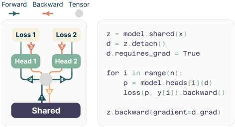Memory-efficient implementation One big challenge in training multi-token predictors is reducing their GPU memory utilization. To see why this is the case, recall that in current LLMs the vocabulary size V is much larger than the dimension d of the latent representation-therefore, logit vectors become the GPU memory usage bottleneck. Naive implementations of multi-token predictors that materialize all logits and their gradients, both of shape ( n, V ) , severely limit the allowable batch-size and average GPU memory utilization. Because of these reasons, in our architecture we propose to carefully adapt the sequence of forward and backward operations, as illustrated in Figure 2. In particular, after the forward pass through the shared trunk f s , we sequentially compute the forward and backward pass of each independent output head f i , accumulating gradients at the trunk. While this creates logits (and their gradients) for the output head f i , these are freed before continuing to the next output head f i +1 , requiring the long-term storage only of the d -dimensional trunk gradient ∂L n /∂f s . In sum, we have reduced the peak GPU memory utilization from O ( nV + d ) to O ( V + d ) , at no expense in runtime (Table S5). Inference During inference time, the most basic use of the proposed architecture is vanilla next-token autoregressive prediction using the next-token prediction head P θ ( x t +1 | x t :1 ) , while discarding all others. However, the additional output heads can be leveraged to speed up decoding from the next-token prediction head with self-speculative decoding methods such as blockwise parallel decoding (Stern et al., 2018)-a variant of speculative decoding (Leviathan et al., 2023) without the need for an additional draft model-and speculative decoding with Medusa-like tree attention (Cai et al., 2024). Figure 2: Order of the forward/backward in an n -token prediction model with n = 2 heads. By performing the forward/backward on the heads in sequential order, we avoid materializing all unembedding layer gradients in memory simultaneously and reduce peak GPU memory usage. <details> <summary>Image 2 Details</summary>  ### Visual Description ## Diagram: Multi-Head Model with Shared Layer and Gradient Flow ### Overview The image depicts a diagram illustrating the forward and backward pass of a multi-head model with a shared layer. The diagram shows the flow of data and gradients through the model, highlighting the shared layer and the individual heads. A code snippet is provided alongside the diagram, likely representing the implementation of the backward pass. ### Components/Axes The diagram consists of the following components: * **Shared Layer:** A blue rounded rectangle labeled "Shared". * **Heads:** Two green rounded rectangles labeled "Head 1" and "Head 2". * **Losses:** Two yellow rounded rectangles labeled "Loss 1" and "Loss 2". * **Arrows:** Arrows indicating the direction of data flow (forward pass - blue) and gradient flow (backward pass - orange). Numbers are placed along the arrows to indicate the order of operations. * **Legend:** A small legend at the top-left corner indicating the meaning of the arrow colors: "Forward" (blue), "Backward" (orange), and "Tensor" (grey). * **Code Snippet:** A block of code written in Python, detailing the backward pass calculation. ### Detailed Analysis or Content Details The diagram illustrates the following flow: 1. **Forward Pass:** Data flows from the "Shared" layer (arrow 1, blue) to both "Head 1" and "Head 2" (arrows 2, blue). 2. **Loss Calculation:** Each head then calculates a loss: "Head 1" to "Loss 1" (arrow 3, blue) and "Head 2" to "Loss 2" (arrow 5, blue). 3. **Backward Pass:** Gradients flow backward from "Loss 1" and "Loss 2". "Loss 1" to "Head 1" (arrow 3, orange), "Loss 2" to "Head 2" (arrow 5, orange). 4. **Gradient Aggregation:** Gradients from both heads converge at the "Shared" layer (arrows 4 and 6, orange). The code snippet details the backward pass: ```python z = model.shared(x) d = z.detach() d.requires_grad = True for i in range(n): p = model.heads[i](d) loss(p, y[i]).backward() z.backward(gradient=d.grad) ``` * `z = model.shared(x)`: The shared layer is applied to the input `x`. * `d = z.detach()`: A detached copy of `z` is created. This prevents gradients from flowing back through `z` directly during the head calculations. * `d.requires_grad = True`: Gradients are enabled for the detached tensor `d`. * `for i in range(n):`: A loop iterates through the heads. * `p = model.heads[i](d)`: Each head `i` is applied to the detached tensor `d`. * `loss(p, y[i]).backward()`: The loss is calculated for the output `p` and the target `y[i]`, and the backward pass is initiated. * `z.backward(gradient=d.grad)`: The gradient is backpropagated through the shared layer `z`, using the gradient of the detached tensor `d`. ### Key Observations * The shared layer is central to the model, receiving input from the data and providing output to multiple heads. * The use of `detach()` in the code suggests a specific gradient flow strategy, likely to avoid unintended gradient accumulation in the shared layer. * The code snippet implements a loop to handle multiple heads, indicating a multi-head architecture. * The numbers on the arrows indicate the order of operations, which is important for understanding the flow of information. ### Interpretation The diagram and code snippet illustrate a common technique in deep learning, particularly in multi-task learning or multi-head attention mechanisms. The shared layer allows for parameter sharing between different heads, potentially improving generalization and reducing the number of parameters. The use of `detach()` and the subsequent gradient manipulation suggest a careful control of gradient flow, which is crucial for training such models effectively. The diagram visually represents the computational graph, making it easier to understand the dependencies between different parts of the model. The code snippet provides a concrete implementation of the backward pass, allowing for a deeper understanding of the gradient calculation process. The overall design suggests a model where different heads can learn different representations from the same shared features, potentially leading to improved performance on multiple tasks. </details> ## 3. Experiments on real data We demonstrate the efficacy of multi-token prediction losses by seven large-scale experiments. Section 3.1 shows how multi-token prediction is increasingly useful when growing the model size. Section 3.2 shows how the additional prediction heads can speed up inference by a factor of 3 × using speculative decoding. Section 3.3 demonstrates how multi-token prediction promotes learning longer-term patterns, a fact most apparent in the extreme case of byte-level tokenization. Section 3.4 shows that 4 -token predictor leads to strong gains with a tokenizer of size 32 k. Section 3.5 illustrates that the benefits of multi-token prediction remain for training runs with multiple epochs. Section 3.6 showcases the rich representations promoted by pretraining with multi-token prediction losses by finetuning on the CodeContests dataset (Li et al., 2022). Section 3.7 shows that the benefits of multi-token prediction carry to natural language models, improving generative evaluations such as summarization, while not regressing significantly on standard benchmarks based on multiple choice questions and negative log-likelihoods. To allow fair comparisons between next-token predictors and n -token predictors, the experiments that follow always compare models with an equal amount of parameters. That is, when we add n -1 layers in future prediction heads, we remove n -1 layers from the shared model trunk. Please refer to Table S14 for the model architectures and to Table S13 for an overview of the hyperparameters we use in our experiments. ## 3.1. Benefits scale with model size To study this phenomenon, we train models of six sizes in the range 300M to 13B parameters from scratch on at least 91B tokens of code. 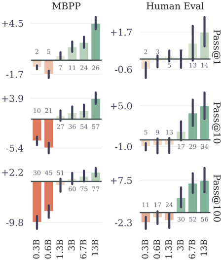The evaluation results in Fig- Figure 3: Results of n -token prediction models on MBPP by model size. We train models of six sizes in the range or 300M to 13B total parameters on code, and evaluate pass@1,10,100 on the MBPP (Austin et al., 2021) and HumanEval (Chen et al., 2021) benchmark with 1000 samples. Multi-token prediction models are worse than the baseline for small model sizes, but outperform the baseline at scale. Error bars are confidence intervals of 90% computed with bootstrapping over dataset samples. <details> <summary>Image 3 Details</summary>  ### Visual Description ## Bar Chart: Model Performance on Programming Tasks ### Overview The image presents a comparative bar chart illustrating the performance of a model (MBPP) and human evaluation on programming tasks, across different model sizes (0.3B to 13B parameters). The performance is measured using three metrics: Pass@1, Pass@10, and Pass@100, representing the probability of generating a correct solution within the first, tenth, and hundredth attempt, respectively. The chart consists of six sub-charts arranged in a 2x3 grid. ### Components/Axes * **X-axis:** Model Size (0.3B, 0.6B, 1.3B, 3B, 6.7B, 13B) - labeled in red. * **Y-axis (MBPP columns):** Performance Score (ranging approximately from -10 to +5). * **Y-axis (Human Eval columns):** Performance Score (ranging approximately from -3 to +8). * **Color Coding:** * Green: Represents positive performance gains. * Red: Represents negative performance or loss. * **Metrics:** * Pass@1: Top row of charts. * Pass@10: Middle row of charts. * Pass@100: Bottom row of charts. * **Titles:** "MBPP" (left column) and "Human Eval" (right column) are placed at the top of their respective columns. * **Labels:** Numerical values are placed above each bar, indicating the specific performance score. ### Detailed Analysis or Content Details **MBPP (Left Column)** * **Pass@1 (Top Row):** * 0.3B: Approximately -1.7, labeled "2". * 0.6B: Approximately -1.7, labeled "5". * 1.3B: Approximately 0.0, labeled "7". * 3B: Approximately +1.5, labeled "11". * 6.7B: Approximately +3.0, labeled "26". * 13B: Approximately +4.5, labeled "26". * Trend: The performance increases steadily from 0.3B to 13B. * **Pass@10 (Middle Row):** * 0.3B: Approximately -5.4, labeled "10". * 0.6B: Approximately -5.4, labeled "21". * 1.3B: Approximately -1.5, labeled "27". * 3B: Approximately +1.5, labeled "36". * 6.7B: Approximately +3.5, labeled "54". * 13B: Approximately +3.9, labeled "57". * Trend: Performance increases with model size, with a more pronounced increase from 1.3B to 3B. * **Pass@100 (Bottom Row):** * 0.3B: Approximately -9.8, labeled "30". * 0.6B: Approximately -9.8, labeled "45". * 1.3B: Approximately -2.0, labeled "51". * 3B: Approximately +0.5, labeled "60". * 6.7B: Approximately +2.0, labeled "75". * 13B: Approximately +2.2, labeled "77". * Trend: Similar to Pass@10, performance improves with model size. **Human Eval (Right Column)** * **Pass@1 (Top Row):** * 0.3B: Approximately -0.6, labeled "2". * 0.6B: Approximately -0.6, labeled "3". * 1.3B: Approximately 0.0, labeled "5". * 3B: Approximately +1.0, labeled "13". * 6.7B: Approximately +1.7, labeled "14". * 13B: Approximately +1.7, labeled "14". * Trend: Performance increases with model size, plateauing at 6.7B and 13B. * **Pass@10 (Middle Row):** * 0.3B: Approximately -1.0, labeled "5". * 0.6B: Approximately -1.0, labeled "9". * 1.3B: Approximately +0.5, labeled "13". * 3B: Approximately +2.0, labeled "17". * 6.7B: Approximately +4.0, labeled "34". * 13B: Approximately +5.0, labeled "34". * Trend: Performance increases with model size, with a significant jump between 3B and 6.7B. * **Pass@100 (Bottom Row):** * 0.3B: Approximately -2.3, labeled "11". * 0.6B: Approximately -2.3, labeled "17". * 1.3B: Approximately +0.5, labeled "24". * 3B: Approximately +3.0, labeled "30". * 6.7B: Approximately +5.5, labeled "52". * 13B: Approximately +7.5, labeled "56". * Trend: Performance increases with model size, with a substantial increase from 3B to 6.7B. ### Key Observations * The model performance (MBPP) consistently improves with increasing model size across all three metrics (Pass@1, Pass@10, Pass@100). * Human evaluation also shows a similar trend of improvement with model size, but the gains appear to plateau at larger model sizes (6.7B and 13B). * The performance gap between the model and human evaluation widens as the model size increases, particularly for Pass@10 and Pass@100. * The red bars indicate that smaller models (0.3B and 0.6B) perform poorly on all metrics, exhibiting negative performance scores. ### Interpretation The data suggests that increasing model size significantly improves performance on programming tasks, as measured by the Pass@k metrics. This is evident in both the MBPP and Human Eval columns. However, the rate of improvement appears to diminish for human evaluation at larger model sizes, indicating a potential limit to the benefits of simply scaling up the model. The widening gap between model and human performance suggests that while the model is becoming more proficient at generating correct solutions, it may still lack the nuanced understanding and problem-solving abilities of a human programmer. The negative performance scores for smaller models highlight the importance of model size for achieving reasonable performance on these tasks. The consistent trend across all metrics reinforces the conclusion that model size is a crucial factor in determining the effectiveness of these models for code generation. The use of different Pass@k metrics allows for a nuanced understanding of the model's ability to generate correct solutions with varying levels of attempts. </details> ure 3 for MBPP (Austin et al., 2021) and HumanEval (Chen et al., 2021) show that it is possible, with the exact same computational budget, to squeeze much more performance out of large language models given a fixed dataset using multi-token prediction. We believe this usefulness only at scale to be a likely reason why multi-token prediction has so far been largely overlooked as a promising training loss for large language model training. ## 3.2. Faster inference We implement greedy self-speculative decoding (Stern et al., 2018) with heterogeneous batch sizes using xFormers (Lefaudeux et al., 2022) and measure decoding speeds of our best 4-token prediction model with 7B parameters on completing prompts taken from a test dataset of code and natural language (Table S2) not seen during training. We observe a speedup of 3 . 0 × on code with an average of 2.5 accepted tokens out of 3 suggestions on code, and of Table 1: Multi-token prediction improves performance and unlocks efficient byte level training. We compare models with 7B parameters trained from scratch on 200B and on 314B bytes of code on the MBPP (Austin et al., 2021), HumanEval (Chen et al., 2021) and APPS (Hendrycks et al., 2021) benchmarks. Multi-token prediction largely outperforms next token prediction on these settings. All numbers were calculated using the estimator from Chen et al. (2021) based on 200 samples per problem. The temperatures were chosen optimally (based on test scores; i.e. these are oracle temperatures) for each model, dataset and pass@k and are reported in Table S12. | Training data | Vocabulary | n | MBPP | MBPP | MBPP | HumanEval | HumanEval | HumanEval | APPS/Intro | APPS/Intro | APPS/Intro | |----------------------|--------------|-----|--------|--------|--------|-------------|-------------|-------------|--------------|--------------|--------------| | Training data | Vocabulary | | @1 | @10 | @100 | @1 | @10 | @100 | @1 | @10 | @100 | | | | 1 | 19.3 | 42.4 | 64.7 | 18.1 | 28.2 | 47.8 | 0.1 | 0.5 | 2.4 | | | | 8 | 32.3 | 50.0 | 69.6 | 21.8 | 34.1 | 57.9 | 1.2 | 5.7 | 14.0 | | | | 16 | 28.6 | 47.1 | 68.0 | 20.4 | 32.7 | 54.3 | 1.0 | 5.0 | 12.9 | | | | 32 | 23.0 | 40.7 | 60.3 | 17.2 | 30.2 | 49.7 | 0.6 | 2.8 | 8.8 | | | | 1 | 30.0 | 53.8 | 73.7 | 22.8 | 36.4 | 62.0 | 2.8 | 7.8 | 17.4 | | | | 2 | 30.3 | 55.1 | 76.2 | 22.2 | 38.5 | 62.6 | 2.1 | 9.0 | 21.7 | | | | 4 | 33.8 | 55.9 | 76.9 | 24.0 | 40.1 | 66.1 | 1.6 | 7.1 | 19.9 | | | | 6 | 31.9 | 53.9 | 73.1 | 20.6 | 38.4 | 63.9 | 3.5 | 10.8 | 22.7 | | | | 8 | 30.7 | 52.2 | 73.4 | 20.0 | 36.6 | 59.6 | 3.5 | 10.4 | 22.1 | | 1T tokens (4 epochs) | | 1 | 40.7 | 65.4 | 83.4 | 31.7 | 57.6 | 83.0 | 5.4 | 17.8 | 34.1 | | 1T tokens (4 epochs) | | 4 | 43.1 | 65.9 | 83.7 | 31.6 | 57.3 | 86.2 | 4.3 | 15.6 | 33.7 | 2 . 7 × on text. On an 8-byte prediction model, the inference speedup is 6 . 4 × (Table S3). Pretraining with multi-token prediction allows the additional heads to be much more accurate than a simple finetuning of a next-token prediction model, thus allowing our models to unlock self-speculative decoding's full potential. ## 3.3. Learning global patterns with multi-byte prediction To show that the next-token prediction task latches to local patterns, we went to the extreme case of byte-level tokenization by training a 7B parameter byte-level transformer on 314B bytes, which is equivalent to around 116B tokens. The 8-byte prediction model achieves astounding improvements compared to next-byte prediction, solving 67% more problems on MBPP pass@1 and 20% more problems on HumanEval pass@1. Multi-byte prediction is therefore a very promising avenue to unlock efficient training of byte-level models. Selfspeculative decoding can achieve speedups of 6 times for the 8-byte prediction model, which would allow to fully compensate the cost of longer byte-level sequences at inference time and even be faster than a next-token prediction model by nearly two times. The 8-byte prediction model is a strong byte-based model, approaching the performance of token-based models despite having been trained on 1 . 7 × less data. ## 3.4. Searching for the optimal n To better understand the effect of the number of predicted tokens, we did comprehensive ablations on models of scale 7B trained on 200B tokens of code. We try n = 1 , 2 , 4 , 6 and 8 in this setting. Results in table 1 show that training with 4-future tokens outperforms all the other models consistently throughout HumanEval and MBPP for pass at 1, 10 and 100 metrics: +3.8%, +2.1% and +3.2% for MBPP and +1.2%, +3.7% and +4.1% for HumanEval. Interestingly, for APPS/Intro, n = 6 takes the lead with +0.7%, +3.0% and +5.3%. It is very likely that the optimal window size depends on input data distribution. As for the byte level models the optimal window size is more consistent (8 bytes) across these benchmarks. ## 3.5. Training for multiple epochs Multi-token training still maintains an edge on next-token prediction when trained on multiple epochs of the same data. The improvements diminish but we still have a +2.4% increase on pass@1 on MBPP and +3.2% increase on pass@100 on HumanEval, while having similar performance for the rest. As for APPS/Intro, a window size of 4 was already not optimal with 200B tokens of training. ## 3.6. Finetuning multi-token predictors Pretrained models with multi-token prediction loss also outperform next-token models for use in finetunings. 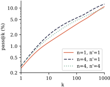We evaluate this by finetuning 7B parameter models from Section 3.3 on the CodeContests dataset (Li et al., 2022). We compare the 4-token prediction model with the next-token prediction baseline, and include a setting where the 4-token prediction model is stripped off its additional prediction heads and finetuned using the classical next-token prediction target. According to the results in Figure 4, both ways of finetuning the 4-token prediction model outperform the next-token prediction model on pass@k across k . This means the models are both better at understanding and solving the task and at generating diverse answers. Note that CodeContests is the most challenging coding benchmark we evaluate in this study. Next-token prediction finetuning on top of 4-token prediction pretraining appears to be the best method overall, in line with the classical paradigm of pretraining with auxiliary tasks followed by task-specific finetuning. Please refer to Appendix F for details. Figure 4: Comparison of finetuning performance on CodeContests. We finetune a 4 -token prediction model on CodeContests (Li et al., 2022) (train split) using n ′ -token prediction as training loss with n ′ = 4 or n ′ = 1 , and compare to a finetuning of the next-token prediction baseline model ( n = n ′ = 1 ). For evaluation, we generate 1000 samples per test problem for each temperature T ∈ { 0 . 5 , 0 . 6 , 0 . 7 , 0 . 8 , 0 . 9 } , and compute pass@k for each value of k and T . Shown is k ↦→ max T pass \_ at( k, T ) , i.e. we grant access to a temperature oracle. We observe that both ways of finetuning the 4-token prediction model outperform the next-token prediction baseline. Intriguingly, using next-token prediction finetuning on top of the 4-token prediction model appears to be the best method overall. <details> <summary>Image 4 Details</summary>  ### Visual Description \n ## Chart: pass@k vs. k for different n and n' values ### Overview The image presents a line chart illustrating the relationship between 'pass@k' (expressed as a percentage) and 'k' for three different combinations of 'n' and 'n'' values. The chart appears to demonstrate how the pass rate changes as 'k' increases, under varying conditions defined by 'n' and 'n''. ### Components/Axes * **X-axis:** Labeled "k". The scale is logarithmic, with markers at 1, 10, 100, and 1000. * **Y-axis:** Labeled "pass@k (%)". The scale is linear, ranging from 0.2 to 10.0, with markers at 0.2, 0.5, 1.0, 2.0, 5.0, and 10.0. * **Legend:** Located in the top-right corner of the chart. It contains the following entries: * Solid line (orange/brown): "n=1, n'=1" * Dashed line (dark blue): "n=4, n'=1" * Dotted line (grey): "n=4, n'=4" ### Detailed Analysis * **n=1, n'=1 (Solid Orange Line):** This line starts at approximately 0.2 at k=1 and increases steadily, curving upwards. At k=10, the value is approximately 1.0%. At k=100, the value is approximately 3.0%. At k=1000, the value reaches approximately 9.5%. * **n=4, n'=1 (Dashed Dark Blue Line):** This line also starts at approximately 0.2 at k=1. It increases more rapidly than the solid orange line. At k=10, the value is approximately 1.8%. At k=100, the value is approximately 5.5%. At k=1000, the value reaches approximately 10.0%. * **n=4, n'=4 (Dotted Grey Line):** This line starts at approximately 0.2 at k=1. It increases at a rate between the solid orange and dashed dark blue lines. At k=10, the value is approximately 1.4%. At k=100, the value is approximately 4.5%. At k=1000, the value reaches approximately 9.8%. ### Key Observations * All three lines start at the same point (approximately 0.2 at k=1). * The dashed dark blue line (n=4, n'=1) consistently shows the highest pass@k values across all 'k' values. * The solid orange line (n=1, n'=1) consistently shows the lowest pass@k values across all 'k' values. * The dotted grey line (n=4, n'=4) falls between the other two lines, indicating a pass rate between the other two conditions. * The rate of increase in pass@k diminishes as 'k' increases for all three lines, suggesting diminishing returns. ### Interpretation The chart demonstrates the impact of 'n' and 'n'' on the 'pass@k' metric. 'pass@k' likely represents the proportion of times a system successfully identifies a correct result within the top 'k' ranked results. 'n' and 'n'' likely represent parameters influencing the system's behavior, potentially related to the number of samples or iterations used. The data suggests that increasing 'n' from 1 to 4, while keeping 'n'' at 1, significantly improves the pass@k rate. Further increasing 'n'' to 4, while keeping 'n' at 4, provides a slight improvement, but not as substantial as the initial increase in 'n'. This could indicate that the initial increase in 'n' has a more significant impact on performance than increasing 'n'' after a certain point. The logarithmic scale on the x-axis suggests that the benefits of increasing 'k' (the number of considered results) become less pronounced as 'k' grows larger. The diminishing returns observed in the curves suggest that there is a point beyond which increasing 'k' does not significantly improve the pass rate. </details> ## 3.7. Multi-token prediction on natural language To evaluate multi-token prediction training on natural language, we train models of size 7B parameters on 200B tokens of natural language with a 4-token, 2-token and nexttoken prediction loss, respectively. In Figure 5, we evaluate the resulting checkpoints on 6 standard NLP benchmarks. 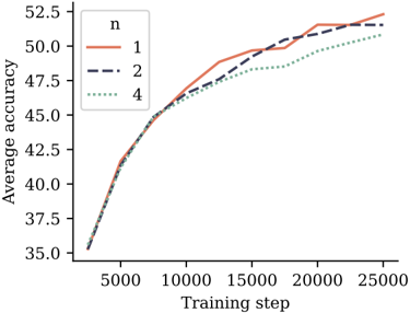On these benchmarks, the 2-future token prediction model performs on par with the next-token prediction baseline Figure 5: Multi-token training with 7B models doesn't improve performance on choice tasks. This figure shows the evolution of average accuracy of 6 standard NLP benchmarks. Detailed results in Appendix G for 7B models trained on 200B tokens of language data. The 2 future token model has the same performance as the baseline and the 4 future token model regresses a bit. Larger model sizes might be necessary to see improvements on these tasks. <details> <summary>Image 5 Details</summary>  ### Visual Description \n ## Line Chart: Average Accuracy vs. Training Step ### Overview This image presents a line chart illustrating the relationship between average accuracy and training step for different values of 'n'. The chart displays three lines, each representing a different 'n' value, showing how accuracy changes as the training progresses. ### Components/Axes * **X-axis:** Training step, ranging from approximately 0 to 25000. * **Y-axis:** Average accuracy, ranging from approximately 35.0 to 52.5. * **Legend:** Located in the top-left corner, identifies the lines based on the value of 'n': * n = 1 (Solid brown line) * n = 2 (Dashed dark blue line) * n = 4 (Dotted light grey line) ### Detailed Analysis * **Line n=1 (Solid brown):** This line starts at approximately 36.0 at a training step of 0, increases steadily, and plateaus around 51.0-51.5 after approximately 15000 training steps. * At 5000 training steps: ~41.0 * At 10000 training steps: ~47.0 * At 15000 training steps: ~49.5 * At 20000 training steps: ~51.0 * At 25000 training steps: ~51.2 * **Line n=2 (Dashed dark blue):** This line also starts at approximately 36.0 at a training step of 0, increases more rapidly than n=1 initially, reaches a peak around 51.5 at approximately 20000 training steps, and then slightly decreases to around 51.0 at 25000 training steps. * At 5000 training steps: ~42.5 * At 10000 training steps: ~48.5 * At 15000 training steps: ~50.0 * At 20000 training steps: ~51.5 * At 25000 training steps: ~51.0 * **Line n=4 (Dotted light grey):** This line starts at approximately 36.0 at a training step of 0, increases at a slower rate than both n=1 and n=2, and plateaus around 48.5-49.0 after approximately 15000 training steps. * At 5000 training steps: ~39.5 * At 10000 training steps: ~45.0 * At 15000 training steps: ~47.5 * At 20000 training steps: ~48.5 * At 25000 training steps: ~49.0 ### Key Observations * All three lines show an increasing trend in average accuracy with increasing training steps, indicating that the model learns over time. * The line for n=2 exhibits the highest accuracy for most of the training process, peaking at approximately 51.5. * The line for n=4 consistently shows the lowest accuracy among the three values of 'n'. * The lines converge as the training step increases, suggesting diminishing returns in accuracy improvement beyond a certain point. ### Interpretation The chart demonstrates the impact of the parameter 'n' on the training process and resulting accuracy. A higher value of 'n' (n=2) appears to lead to faster learning and higher accuracy, at least up to a certain training step. However, the difference in accuracy between n=1 and n=2 is relatively small, and the performance of n=4 is significantly lower. This suggests that 'n' may represent a complexity parameter or a resource allocation factor. The plateauing of all lines indicates that the model is approaching its maximum achievable accuracy with the given training data and configuration. The slight decrease in accuracy for n=2 at the very end of the training process could indicate overfitting, where the model begins to perform worse on unseen data. Further investigation would be needed to determine the optimal value of 'n' and whether additional training or regularization techniques could improve performance. </details> throughout training. The 4-future token prediction model suffers a performance degradation. Detailed numbers are reported in Appendix G. However, we do not believe that multiple-choice and likelihood-based benchmarks are suited to effectively discern generative capabilities of language models. In order to avoid the need for human annotations of generation quality or language model judges-which comes with its own pitfalls, as pointed out by Koo et al. (2023)-we conduct evaluations on summarization and natural language mathematics benchmarks and compare pretrained models with training sets sizes of 200B and 500B tokens and with nexttoken and multi-token prediction losses, respectively. 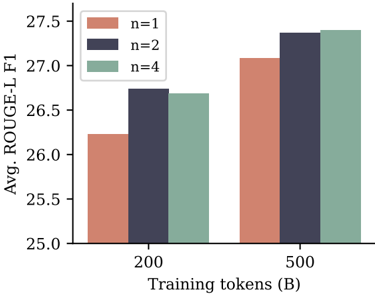For summarization, we use eight benchmarks where ROUGE metrics (Lin, 2004) with respect to a ground-truth summary allow automatic evaluation of generated texts. We finetune each pretrained model on each benchmark's training dataset for three epochs and select the checkpoint with the highest ROUGE-L F 1 score on the validation dataset. Figure 6 shows that multi-token prediction models with both n = 2 and n = 4 improve over the next-token baseline in ROUGE-L F 1 scores for both training dataset sizes, with the performance gap shrinking with larger dataset size. All metrics can be found in Appendix H. For natural language mathematics, we evaluate the pretrained models in 8-shot mode on the GSM8K benchmark (Cobbe et al., 2021) and measure accuracy of the final answer produced after a chain-of-thought elicited by the fewshot examples. We evaluate pass@k metrics to quantify diversity and correctness of answers like in code evaluations Figure 6: Performance on abstractive text summarization. Average ROUGE-L (longest common subsequence overlap) F 1 score for 7B models trained on 200B and 500B tokens of natural language on eight summarization benchmarks. We finetune the respective models on each task's training data separately for three epochs and select the checkpoints with highest ROUGE-L F 1 validation score. Both n = 2 and n = 4 multi-token prediction models have an advantage over next-token prediction models. Individual scores per dataset and more details can be found in Appendix H. <details> <summary>Image 6 Details</summary>  ### Visual Description \n ## Bar Chart: ROUGE-L F1 Score vs. Training Tokens ### Overview This bar chart displays the average ROUGE-L F1 score for different values of 'n' (1, 2, and 4) at two training token sizes: 200B and 500B. The chart visually compares the performance of each 'n' value at each training token size. ### Components/Axes * **X-axis:** Training tokens (B) - with markers at 200 and 500. * **Y-axis:** Avg. ROUGE-L F1 - ranging from approximately 25.0 to 27.5. * **Legend:** Located in the top-left corner, defining the colors for each 'n' value: * n=1 (Light Red/Salmon) * n=2 (Dark Blue/Navy) * n=4 (Light Green/Seafoam) ### Detailed Analysis The chart consists of six bars, representing the ROUGE-L F1 scores for each combination of 'n' and training token size. * **n=1:** * At 200B training tokens: Approximately 26.2. The bar extends from roughly 25.9 to 26.5. * At 500B training tokens: Approximately 27.0. The bar extends from roughly 26.8 to 27.2. * **n=2:** * At 200B training tokens: Approximately 26.7. The bar extends from roughly 26.5 to 26.9. * At 500B training tokens: Approximately 27.3. The bar extends from roughly 27.1 to 27.5. * **n=4:** * At 200B training tokens: Approximately 26.6. The bar extends from roughly 26.4 to 26.8. * At 500B training tokens: Approximately 27.2. The bar extends from roughly 27.0 to 27.4. All three 'n' values show an increase in ROUGE-L F1 score when the training token size increases from 200B to 500B. The 'n=2' consistently has the highest ROUGE-L F1 score at both training token sizes. ### Key Observations * Increasing the training token size consistently improves the ROUGE-L F1 score for all 'n' values. * 'n=2' consistently outperforms 'n=1' and 'n=4' at both training token sizes. * The difference in performance between 'n=1' and 'n=4' is relatively small. ### Interpretation The data suggests that increasing the number of training tokens generally leads to improved performance, as measured by the ROUGE-L F1 score. The optimal value for 'n' appears to be 2, as it consistently yields the highest scores. This could indicate that using a larger context window (represented by 'n') during training is beneficial up to a certain point, but beyond that, the gains diminish or even decrease. The relatively small difference between 'n=1' and 'n=4' suggests that there may be diminishing returns from increasing the context window beyond a certain size. The ROUGE-L F1 score is a metric for evaluating the quality of text summarization or machine translation, so this data likely relates to the performance of a language model on such tasks. The 'B' in the x-axis label indicates that the training token size is measured in billions of tokens. </details> and use sampling temperatures between 0.2 and 1.4. The results are depicted in Figure S13 in Appendix I. For 200B training tokens, the n = 2 model clearly outperforms the next-token prediction baseline, while the pattern reverses after 500B tokens and n = 4 is worse throughout. ## 4. Ablations on synthetic data What drives the improvements in downstream performance of multi-token prediction models on all of the tasks we have considered? By conducting toy experiments on controlled training datasets and evaluation tasks, we demonstrate that multi-token prediction leads to qualitative changes in model capabilities and generalization behaviors . In particular, Section 4.1 shows that for small model sizes, induction capability -as discussed by Olsson et al. (2022)-either only forms when using multi-token prediction as training loss, or it is vastly improved by it. Moreover, Section 4.2 shows that multi-token prediction improves generalization on an arithmetic task, even more so than tripling model size. ## 4.1. Induction capability Induction describes a simple pattern of reasoning that completes partial patterns by their most recent continuation (Olsson et al., 2022). In other words, if a sentence contains 'AB' and later mentions 'A', induction is the prediction that the continuation is 'B'. 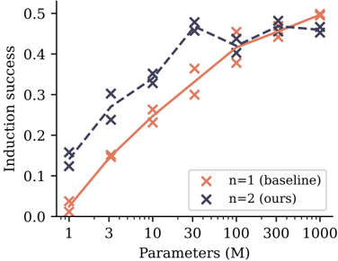We design a setup to measure induction Figure 7: Induction capability of n -token prediction models. Shown is accuracy on the second token of two token names that have already been mentioned previously. Shown are numbers for models trained with a next-token and a 2-token prediction loss, respectively, with two independent runs each. The lines denote per-loss averages. For small model sizes, next-token prediction models learn practically no or significantly worse induction capability than 2-token prediction models, with their disadvantage disappearing at the size of 100M nonembedding parameters. <details> <summary>Image 7 Details</summary>  ### Visual Description \n ## Line Chart: Induction Success vs. Parameters ### Overview This image presents a line chart illustrating the relationship between the number of parameters (in millions) and induction success. Two data series are plotted, representing different values of 'n' (n=1 and n=2). The chart demonstrates how induction success changes as the number of parameters increases for both scenarios. ### Components/Axes * **X-axis:** "Parameters (M)" - Scale ranges from approximately 1 to 1000, with markers at 1, 3, 10, 30, 100, 300, and 1000. * **Y-axis:** "Induction success" - Scale ranges from 0.0 to 0.5, with markers at 0.0, 0.1, 0.2, 0.3, 0.4, and 0.5. * **Legend:** Located in the top-right corner. * "n = 1 (baseline)" - Represented by an orange 'x' marker. * "n = 2 (ours)" - Represented by a dark blue 'x' marker. ### Detailed Analysis **Data Series 1: n = 1 (baseline) - Orange Line** The orange line representing n=1 exhibits an upward trend initially, then plateaus. * At 1 M parameters, induction success is approximately 0.05. * At 3 M parameters, induction success is approximately 0.15. * At 10 M parameters, induction success is approximately 0.30. * At 30 M parameters, induction success is approximately 0.38. * At 100 M parameters, induction success is approximately 0.42. * At 300 M parameters, induction success is approximately 0.45. * At 1000 M parameters, induction success is approximately 0.46. **Data Series 2: n = 2 (ours) - Dark Blue Line** The dark blue line representing n=2 shows a steeper upward trend than the orange line, reaching a peak and then slightly decreasing. * At 1 M parameters, induction success is approximately 0.13. * At 3 M parameters, induction success is approximately 0.25. * At 10 M parameters, induction success is approximately 0.37. * At 30 M parameters, induction success is approximately 0.44. * At 100 M parameters, induction success is approximately 0.47. * At 300 M parameters, induction success is approximately 0.48. * At 1000 M parameters, induction success is approximately 0.47. ### Key Observations * The "n=2" data series consistently outperforms the "n=1" data series across all parameter values. * Both data series demonstrate diminishing returns as the number of parameters increases beyond 300 M. The improvement in induction success becomes marginal. * The "n=2" series reaches its peak performance around 300 M parameters, then slightly declines at 1000 M. ### Interpretation The chart suggests that increasing the number of parameters generally improves induction success, but the benefit diminishes with larger parameter counts. The "n=2" configuration ("ours") consistently achieves higher induction success than the "n=1" baseline, indicating that the proposed method (represented by n=2) is more effective. The slight decline in performance for the "n=2" series at 1000 M parameters could indicate overfitting or the point of diminishing returns for this specific model configuration. The data implies that there is an optimal parameter range for maximizing induction success, and exceeding that range may not yield significant improvements and could even lead to a slight decrease in performance. The chart provides evidence supporting the effectiveness of the "ours" method (n=2) over the baseline (n=1) in achieving higher induction success, particularly within the range of 1 to 300 million parameters. </details> capability in a controlled way. Training small models of sizes 1M to 1B nonembedding parameters on a dataset of children stories, we measure induction capability by means of an adapted test set: in 100 stories from the original test split, we replace the character names by randomly generated names that consist of two tokens with the tokenizer we employ. Predicting the first of these two tokens is linked to the semantics of the preceding text, while predicting the second token of each name's occurrence after it has been mentioned at least once can be seen as a pure induction task. In our experiments, we train for up to 90 epochs and perform early stopping with respect to the test metric (i.e. we allow an epoch oracle). Figure 7 reports induction capability as measured by accuracy on the names' second tokens in relation to model size for two runs with different seeds. We find that 2-token prediction loss leads to a vastly improved formation of induction capability for models of size 30M nonembedding parameters and below, with their advantage disappearing for sizes of 100M nonembedding parameters and above. 1 We interpret this finding as follows: multitoken prediction losses help models to learn transferring information across sequence positions, which lends itself to the formation of induction heads and other in-context learning mechanisms. However, once induction capability has been formed, these learned features transform induction 1 Note that a perfect score is not reachable in this benchmark as some of the tokens in the names in the evaluation dataset never appear in the training data, and in our architecture, embedding and unembedding parameters are not linked. 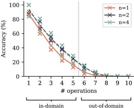Figure 8: Accuracy on a polynomial arithmetic task with varying number of operations per expression. Training with multi-token prediction losses increases accuracy across task difficulties. In particular, it also significantly improves out-of-domain generalization performance, albeit at a low absolute level. Tripling the model size, on the other hand, has a considerably smaller effect than replacing next-token prediction with multi-token prediction loss (Figure S16). Shown are two independent runs per configuration with 100M parameter models. <details> <summary>Image 8 Details</summary>  ### Visual Description \n ## Line Chart: </details> into a task that can be solved locally at the current token and learned with next-token prediction alone. From this point on, multi-token prediction actually hurts on this restricted benchmark-but we surmise that there are higher forms of in-context reasoning to which it further contributes, as evidenced by the results in Section 3.1. In Figure S14, we provide evidence for this explanation: replacing the children stories dataset by a higher-quality 9:1 mix of a books dataset with the children stories, we enforce the formation of induction capability early in training by means of the dataset alone. By consequence, except for the two smallest model sizes, the advantage of multi-token prediction on the task disappears: feature learning of induction features has converted the task into a pure next-token prediction task. ## 4.2. Algorithmic reasoning Algorithmic reasoning tasks allow to measure more involved forms of in-context reasoning than induction alone. We train and evaluate models on a task on polynomial arithmetic in the ring F 7 [ X ] / ( X 5 ) with unary negation, addition, multiplication and composition of polynomials as operations. The coefficients of the operands and the operators are sampled uniformly. The task is to return the coefficients of the polynomials corresponding to the resulting expressions. The number m of operations contained in the expressions is selected uniformly from the range from 1 to 5 at training time, and can be used to adjust the difficulty of both in-domain ( m ≤ 5 ) and out-of-domain ( m> 5 ) generalization evaluations. The evaluations are conducted with greedy sampling on a fixed test set of 2000 samples per number of operations. We train models of two small sizes with 30M and 100M nonembedding parameters, respectively. This simulates the conditions of large language models trained on massive text corpora which are likewise under-parameterized and unable to memorize their entire training datasets. Multi-token prediction improves algorithmic reasoning capabilities as measured by this task across task difficulties (Figure 8). In particular, it leads to impressive gains in out-of-distribution generalization, despite the low absolute numbers. Increasing the model size from 30M to 100M parameters, on the other hand, does not improve evaluation accuracy as much as replacing next-token prediction by multi-token prediction does (Figure S16). In Appendix K, we furthermore show that multi-token prediction models retain their advantage over next-token prediction models on this task when trained and evaluated with pause tokens (Goyal et al., 2023). ## 5. Why does it work? Some speculation Why does multi-token prediction afford superior performance on coding evaluation benchmarks, and on small algorithmic reasoning tasks? Our intuition, developed in this section, is that multi-token prediction mitigates the distributional discrepancy between training-time teacher forcing and inference-time autoregressive generation. We support this view with an illustrative argument on the implicit weights multi-token prediction assigns to tokens depending on their relevance for the continuation of the text, as well as with an information-theoretic decomposition of multi-token prediction loss. ## 5.1. Lookahead reinforces choice points Not all token decisions are equally important for generating useful texts from language models (Bachmann and Nagarajan, 2024; Lin et al., 2024). While some tokens allow stylistic variations that do not constrain the remainder of the text, others represent choice points that are linked with higher-level semantic properties of the text and may decide whether an answer is perceived as useful or derailing . 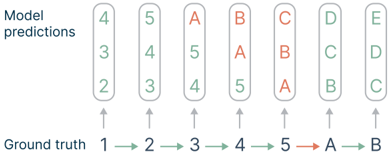Multi-token prediction implicitly assigns weights to training tokens depending on how closely they are correlated with their successors. As an illustrative example, consider the sequence depicted in Figure 9 where one transition is a hard-to-predict choice point while the other transitions are considered 'inconsequential'. Inconsequential transitions following a choice point are likewise hard to predict in advance. By marking and counting loss terms, we find that Figure 9: Multi-token prediction loss assigns higher implicit weights to consequential tokens. Shown is a sequence in which all transitions except '5 → A' are easy to predict, alongside the corresponding prediction targets in 3-token prediction. Since the consequences of the difficult transition '5 → A' are likewise hard to predict, this transition receives a higher implicit weight in the overall loss via its correlates '3 → A', ..., '5 → C'. <details> <summary>Image 9 Details</summary>  ### Visual Description \n ## Diagram: Model Prediction vs. Ground Truth ### Overview The image presents a diagram comparing model predictions to the ground truth for a sequence of data points. It visually represents the accuracy of a model's predictions against the actual values. The diagram consists of paired vertical rectangles, with the top rectangle representing the model's prediction and the bottom rectangle representing the ground truth. Arrows connect the ground truth values to their corresponding model predictions. ### Components/Axes The diagram has two main sections: * **Model predictions:** Labeled on the left side of the image. * **Ground truth:** Labeled at the bottom of the image. The ground truth values are numerical (1, 2, 3, 4, 5) and alphabetical (A, B). The model predictions also consist of numerical (2, 3, 4, 5) and alphabetical (A, B, C, D, E) values. Arrows point upwards from each ground truth value to its corresponding model prediction. ### Detailed Analysis The diagram shows the following pairings of ground truth and model predictions: 1. Ground Truth: 1 -> Model Prediction: 4 2. Ground Truth: 2 -> Model Prediction: 5 3. Ground Truth: 3 -> Model Prediction: A 4. Ground Truth: 4 -> Model Prediction: B 5. Ground Truth: 5 -> Model Prediction: C 6. Ground Truth: A -> Model Prediction: D 7. Ground Truth: B -> Model Prediction: E The values within each vertical rectangle are arranged vertically, suggesting a scale or ordering. The numerical values in the "Model predictions" rectangles range from approximately 2 to 5. The alphabetical values are A, B, C, D, and E. ### Key Observations * The model consistently mispredicts the ground truth values. There are no correct predictions. * The model appears to consistently overestimate the numerical values (1 and 2 are predicted as 4 and 5 respectively). * The model's predictions for the alphabetical values also deviate from the ground truth. * There is a clear pattern of systematic error in the model's predictions. ### Interpretation The diagram demonstrates a significant discrepancy between the model's predictions and the actual ground truth values. The model consistently makes incorrect predictions, indicating a potential issue with the model's training, architecture, or the data it was trained on. The systematic nature of the errors suggests that the model may be biased or have a limited understanding of the underlying relationships in the data. The consistent overestimation of numerical values could indicate a scaling issue or a bias towards higher values. Further investigation is needed to identify the root cause of these errors and improve the model's performance. The diagram serves as a clear visual representation of the model's shortcomings and highlights the need for further refinement. </details> n -token prediction associates a weight of n ( n +1) 2 to choice points via their correlates, and a smaller weight of n to inconsequential points. Please refer to Appendix L.3 for more details. Generally, we believe that the quality of text generations depends on picking the right decisions at choice points, and that n -token prediction losses promote those. ## 5.2. Information-theoretic argument Language models are typically trained by teacher-forcing, where the model receives the ground truth for each future token during training. However, during test time generation is unguided and autoregressive, whereby errors accumulate. Teacher-forcing, we argue, encourages models to focus on predicting well in the very short term, at the potential expense of ignoring longer-term dependencies in the overall structure of the generated sequence. To illustrate the impact of multi-token prediction, consider the following information-theoretic argument. Here, X denotes the next future token, and Y the second-next future token. The production of both of these tokens is conditioned on some observed, input context C , that we omit from our equations for simplicity. When placed before token X , vanilla next-token prediction concerns the quantity H ( X ) , while multi-token prediction with n = 2 aims at H ( X ) + H ( Y ) . We decompose these two quantities as: $$\begin{aligned} H ( X ) = H ( X | Y ) + H ( Y | X ) , \\ H ( X ) + H ( Y ) = H ( X | Y ) + H ( Y | X ). \end{aligned}$$ By discarding the term H ( Y | X ) -which appears again when predicting at the following position-we observe that 2-token prediction increases the importance of I ( X ; Y ) by a factor of 2 . So, multi-token predictors are more accurate at predicting tokens X that are of relevance for the remainder of the text to come. In Appendix L.2, we give a relative version of the above equations that shows the increased weight of relative mutual information in a loss decomposition of 2-token prediction loss. ## 6. Related work Language modeling losses Dong et al. (2019) and Tay et al. (2022) train on a mixture of denoising tasks with different attention masks (full, causal and prefix attention) to bridge the performance gap with next token pretraining on generative tasks. Tay et al. (2022) uses the span corruption objective, which replaces spans of tokens with special tokens for the encoder and the decoder then predicts the contents of those spans. Unlike UniLM, this allows full causal training with teacher forcing. Similarly, Yang et al. (2019) train on permuted sequences, while conserving the original positional embeddings, effectively training the model to predict various parts of the sequence given a mix of past and future information. This permuted language modeling is the closest task to ours since it allows predicting beyond the next token. However all of these language modeling tasks train on a small percentage of the input text: on average only 15% of the tokens are backwarded through. For Dong et al. (2019), where the masking is done in BERT style, it is hard to mask more than 15% since it destroys too much information. For Tay et al. (2022), it is technically possible to have a larger proportion but in practice, the settings used have between 15% and 25% of masked tokens. (Yang et al., 2019) also makes it possible to train on the whole sequence since it is only permuted, and no information is lost. Yet, in practice, since the completely random permutation is very hard to reconstruct, only 15% are predicted for training stability reasons. Multi-token prediction in language modelling Qi et al. (2020) argue that multi-token prediction encourages planning, improves representations and prevents the overfitting on local patterns that can result from teacher-forced training. However, their technical approach replicates the residual stream n -fold while ours allows for compute-matched comparisons and makes the residual representations participate more directly in the auxiliary loss terms. Stern et al. (2018) and Cai et al. (2024) propose model finetunings with multitoken prediction for faster inference but do not study the effects of such a loss during pretraining. Pal et al. (2023) use probing methods to show that next-token prediction models are able to predict additional consecutive tokens to a certain extent, but less so than our models which are specifically trained for this task. Jianyu Zhang (2024) observe improvements in language modelling tasks with multi-label binary classification over the occurrence of vocabulary words in the future as an auxiliary learning task. Self-speculative decoding Stern et al. (2018) are, to the best of our knowledge, the first to suggest a speculative decoding scheme for faster inference. Our architecture replaces their linear prediction heads by transformer layers, but is otherwise similar. By reorganizing the order of the forward/backward, we can use all loss terms instead of stochastically picking one head for loss computation. Cai et al. (2024) present a more elaborate self-speculative decoding scheme that uses the topk predictions of each head instead of the best one only. It can be used with the multi-token prediction models we train. Multi-target prediction Multi-task learning is the paradigm of training neural networks jointly on several tasks to improve performance on the tasks of interest (Caruana, 1997). Learning with such auxiliary tasks allows models to exploit dependencies between target variables and can even be preferable in the case of independent targets (Waegeman et al., 2019). While more specifically tailored architectures for multi-target prediction are conceivable (SpyromitrosXioufis et al., 2016; Read et al., 2021), modern deep learning approaches usually rely on large shared model trunks with separate prediction heads for the respective tasks (Caruana, 1997; Silver et al., 2016; Lample et al., 2022) like we do. Multi-target prediction has been shown to be a successful strategy in various domains, e.g. for learning time series prediction with more distant time steps in the future as auxiliary targets (Vapnik and Vashist, 2009) or for learning from videos with several future frames (Mathieu et al., 2016; Srivastava et al., 2016) or representations of future frames (Vondrick et al., 2016) as auxiliary targets. ## 7. Conclusion Wehave proposed multi-token prediction as an improvement over next-token prediction in training language models for generative or reasoning tasks. Our experiments (up to 7B parameters and 1T tokens) show that this is increasingly useful for larger models and in particular show strong improvements for code tasks. We posit that our method reduces distribution mismatch between teacher-forced training and autoregressive generation. When used with speculative decoding, exact inference gets 3 times faster. In future work we would like to better understand how to automatically choose n in multi-token prediction losses. One possibility to do so is to use loss scales and loss balancing (Défossez et al., 2022). Also, optimal vocabulary sizes for multi-token prediction are likely different from those for next-token prediction, and tuning them could lead to better results, as well as improved trade-offs between compressed sequence length and compute-per-byte expenses. Finally, we would like to develop improved auxiliary prediction losses that operate in embedding spaces (LeCun, 2022). ## Impact statement The goal of this paper is to make language models more compute and data efficient. While this may in principle reduce the ecological impact of training LLMs, we shall be careful about rebound effects . All societal advantages, as well as risks, of LLMs should be considered while using this work. ## Environmental impact In aggregate, training all models reported in the paper required around 500K GPU hours of computation on hardware of type A100-80GB and H100. Estimated total emissions were around 50 tCO2eq, 100% of which were offset by Meta's sustainability program. ## Acknowledgements We thank Jianyu Zhang, Léon Bottou, Emmanuel Dupoux, Pierre-Emmanuel Mazaré, Yann LeCun, Quentin Garrido, Megi Dervishi, Mathurin Videau and Timothée Darcet and other FAIR PhD students and CodeGen team members for helpful discussions. We thank Jonas Gehring for his technical expertise and the original Llama team and xFormers team for enabling this kind of research. ## References - Jacob Austin, Augustus Odena, Maxwell Nye, Maarten Bosma, Henryk Michalewski, David Dohan, Ellen Jiang, Carrie Cai, Michael Terry, Quoc Le, et al. Program synthesis with large language models. arXiv preprint arXiv:2108.07732 , 2021. - Gregor Bachmann and Vaishnavh Nagarajan. The pitfalls of next-token prediction, 2024. - Samy Bengio, Oriol Vinyals, Navdeep Jaitly, and Noam Shazeer. Scheduled sampling for sequence prediction with recurrent neural networks, 2015. Yonatan Bisk, Rowan Zellers, Ronan Le Bras, Jianfeng Gao, and Yejin Choi. Piqa: Reasoning about physical commonsense in natural language, 2019. - Tianle Cai, Yuhong Li, Zhengyang Geng, Hongwu Peng, Jason D. Lee, Deming Chen, and Tri Dao. Medusa: Simple llm inference acceleration framework with multiple decoding heads, 2024. Rich Caruana. Multitask learning. Machine learning , 28: 41-75, 1997. - Mark Chen, Jerry Tworek, Heewoo Jun, Qiming Yuan, Henrique Ponde, Jared Kaplan, Harri Edwards, Yura Burda, Nicholas Joseph, Greg Brockman, et al. Evaluating large language models trained on code. arXiv preprint arXiv:2107.03374 , 2021. - Nakhun Chumpolsathien. Using knowledge distillation from keyword extraction to improve the informativeness of neural cross-lingual summarization. Master's thesis, Beijing Institute of Technology, 2020. - Karl Cobbe, Vineet Kosaraju, Mohammad Bavarian, Mark Chen, Heewoo Jun, Lukasz Kaiser, Matthias Plappert, Jerry Tworek, Jacob Hilton, Reiichiro Nakano, et al. Training verifiers to solve math word problems. arXiv preprint arXiv:2110.14168 , 2021. - Li Dong, Nan Yang, Wenhui Wang, Furu Wei, Xiaodong Liu, Yu Wang, Jianfeng Gao, Ming Zhou, and Hsiao-Wuen Hon. Unified language model pre-training for natural language understanding and generation. In Proceedings of the 33rd International Conference on Neural Information Processing Systems , pages 13063-13075, 2019. - Alexandre Défossez, Jade Copet, Gabriel Synnaeve, and Yossi Adi. High fidelity neural audio compression. arXiv preprint arXiv:2210.13438 , 2022. - Moussa Kamal Eddine, Antoine J. P. Tixier, and Michalis Vazirgiannis. Barthez: a skilled pretrained french sequence-to-sequence model, 2021. - Alexander R. Fabbri, Irene Li, Tianwei She, Suyi Li, and Dragomir R. Radev. Multi-news: a large-scale multidocument summarization dataset and abstractive hierarchical model, 2019. Mehrdad Farahani. Summarization using bert2bert model on wikisummary dataset. https://github.com/m3hrdadfi/wikisummary, 2020. Mehrdad Farahani, Mohammad Gharachorloo, and Mohammad Manthouri. Leveraging parsbert and pretrained mt5 for persian abstractive text summarization. In 2021 26th International Computer Conference, Computer Society of Iran (CSICC) . IEEE, March 2021. doi: 10.1109/ csicc52343.2021.9420563. URL http://dx.doi. org/10.1109/CSICC52343.2021.9420563 . - Michael C Frank. Bridging the data gap between children and large language models. Trends in Cognitive Sciences , 2023. Bogdan Gliwa, Iwona Mochol, Maciej Biesek, and Aleksander Wawer. Samsum corpus: A human-annotated dialogue dataset for abstractive summarization. In Proceedings of the 2nd Workshop on New Frontiers in Summarization . Association for Computational Linguistics, 2019. doi: 10.18653/v1/d19-5409. URL http: //dx.doi.org/10.18653/v1/D19-5409 . - Sachin Goyal, Ziwei Ji, Ankit Singh Rawat, Aditya Krishna Menon, Sanjiv Kumar, and Vaishnavh Nagarajan. Think before you speak: Training language models with pause tokens, 2023. - Dan Hendrycks, Steven Basart, Saurav Kadavath, Mantas Mazeika, Akul Arora, Ethan Guo, Collin Burns, Samir Puranik, Horace He, Dawn Song, et al. Measuring coding challenge competence with apps. arXiv preprint arXiv:2105.09938 , 2021. - Ari Holtzman, Jan Buys, Li Du, Maxwell Forbes, and Yejin Choi. The curious case of neural text degeneration, 2020. - Jianyu Zhang Leon Bottou. Multi-label classification as an auxiliary loss for language modelling. personal communication, 2024. - Mandar Joshi, Eunsol Choi, Daniel S. Weld, and Luke Zettlemoyer. Triviaqa: A large scale distantly supervised challenge dataset for reading comprehension, 2017. Diederik Kingma and Jimmy Ba. Adam: A method for stochastic optimization. ICLR , 2015. Ryan Koo, Minhwa Lee, Vipul Raheja, Jong Inn Park, Zae Myung Kim, and Dongyeop Kang. Benchmarking cognitive biases in large language models as evaluators. arXiv preprint arXiv:2309.17012 , 2023. Tom Kwiatkowski, Jennimaria Palomaki, Olivia Redfield, Michael Collins, Ankur Parikh, Chris Alberti, Danielle Epstein, Illia Polosukhin, Matthew Kelcey, Jacob Devlin, Kenton Lee, Kristina N. Toutanova, Llion Jones, MingWei Chang, Andrew Dai, Jakob Uszkoreit, Quoc Le, and Slav Petrov. Natural questions: a benchmark for question answering research. Transactions of the Association of Computational Linguistics , 2019. - Guillaume Lample, Marie-Anne Lachaux, Thibaut Lavril, Xavier Martinet, Amaury Hayat, Gabriel Ebner, Aurélien Rodriguez, and Timothée Lacroix. Hypertree proof search for neural theorem proving, 2022. - Yann LeCun. A path towards autonomous machine intelligence version 0.9. 2, 2022-06-27. Open Review , 62(1), 2022. - Benjamin Lefaudeux, Francisco Massa, Diana Liskovich, Wenhan Xiong, Vittorio Caggiano, Sean Naren, Min Xu, Jieru Hu, Marta Tintore, Susan Zhang, Patrick Labatut, and Daniel Haziza. xformers: A modular and hackable transformer modelling library. https://github. com/facebookresearch/xformers , 2022. - Yaniv Leviathan, Matan Kalman, and Yossi Matias. Fast inference from transformers via speculative decoding, 2023. - Yujia Li, David Choi, Junyoung Chung, Nate Kushman, Julian Schrittwieser, Rémi Leblond, Tom Eccles, James Keeling, Felix Gimeno, Agustin Dal Lago, et al. Competition-level code generation with alphacode. Science , 378(6624):1092-1097, 2022. - Chin-Yew Lin. ROUGE: A package for automatic evaluation of summaries. In Text Summarization Branches Out , pages 74-81, Barcelona, Spain, July 2004. Association for Computational Linguistics. URL https: //aclanthology.org/W04-1013 . - Zhenghao Lin, Zhibin Gou, Yeyun Gong, Xiao Liu, Yelong Shen, Ruochen Xu, Chen Lin, Yujiu Yang, Jian Jiao, Nan Duan, and Weizhu Chen. Rho-1: Not all tokens are what you need, 2024. - Ilya Loshchilov and Frank Hutter. Sgdr: Stochastic gradient descent with warm restarts, 2017. - Ilya Loshchilov and Frank Hutter. Decoupled weight decay regularization, 2019. - Michael Mathieu, Camille Couprie, and Yann LeCun. Deep multi-scale video prediction beyond mean square error, 2016. - Ramesh Nallapati, Bowen Zhou, Cicero Nogueira dos santos, Caglar Gulcehre, and Bing Xiang. Abstractive text - summarization using sequence-to-sequence rnns and beyond, 2016. Shashi Narayan, Shay B. Cohen, and Mirella Lapata. Don't give me the details, just the summary! topic-aware convolutional neural networks for extreme summarization, 2018. Catherine Olsson, Nelson Elhage, Neel Nanda, Nicholas Joseph, Nova DasSarma, Tom Henighan, Ben Mann, Amanda Askell, Yuntao Bai, Anna Chen, Tom Conerly, Dawn Drain, Deep Ganguli, Zac Hatfield-Dodds, Danny Hernandez, Scott Johnston, Andy Jones, Jackson Kernion, Liane Lovitt, Kamal Ndousse, Dario Amodei, Tom Brown, Jack Clark, Jared Kaplan, Sam McCandlish, and Chris Olah. In-context learning and induction heads. Transformer Circuits Thread , 2022. https://transformer-circuits.pub/2022/in-contextlearning-and-induction-heads/index.html. OpenAI. Gpt-4 technical report, 2023. Long Ouyang, Jeff Wu, Xu Jiang, Diogo Almeida, Carroll L. Wainwright, Pamela Mishkin, Chong Zhang, Sandhini Agarwal, Katarina Slama, Alex Ray, John Schulman, Jacob Hilton, Fraser Kelton, Luke Miller, Maddie Simens, Amanda Askell, Peter Welinder, Paul Christiano, Jan Leike, and Ryan Lowe. Training language models to follow instructions with human feedback, 2022. - Koyena Pal, Jiuding Sun, Andrew Yuan, Byron C. Wallace, and David Bau. Future lens: Anticipating subsequent tokens from a single hidden state, 2023. - Weizhen Qi, Yu Yan, Yeyun Gong, Dayiheng Liu, Nan Duan, Jiusheng Chen, Ruofei Zhang, and Ming Zhou. Prophetnet: Predicting future n-gram for sequence-tosequence pre-training, 2020. - Jesse Read, Bernhard Pfahringer, Geoffrey Holmes, and Eibe Frank. Classifier chains: A review and perspectives. Journal of Artificial Intelligence Research , 70:683-718, 2021. - Melissa Roemmele, Cosmin Adrian Bejan, and Andrew S Gordon. Choice of plausible alternatives: An evaluation of commonsense causal reasoning. In 2011 AAAI Spring Symposium Series , 2011. - Maarten Sap, Hannah Rashkin, Derek Chen, Ronan LeBras, and Yejin Choi. Socialiqa: Commonsense reasoning about social interactions, 2019. - David Silver, Aja Huang, Chris J Maddison, Arthur Guez, Laurent Sifre, George Van Den Driessche, Julian Schrittwieser, Ioannis Antonoglou, Veda Panneershelvam, Marc Lanctot, et al. Mastering the game of go with deep neural networks and tree search. nature , 529(7587): 484-489, 2016.