2405.00451v2

# Monte Carlo Tree Search Boosts Reasoning via Iterative Preference Learning > Correspondence to: Yuxi Xie (xieyuxi@u.nus.edu) and Anirudh Goyal (anirudhgoyal9119@gmail.com). Abstract We introduce an approach aimed at enhancing the reasoning capabilities of Large Language Models (LLMs) through an iterative preference learning process inspired by the successful strategy employed by AlphaZero. Our work leverages Monte Carlo Tree Search (MCTS) to iteratively collect preference data, utilizing its look-ahead ability to break down instance-level rewards into more granular step-level signals. To enhance consistency in intermediate steps, we combine outcome validation and stepwise self-evaluation, continually updating the quality assessment of newly generated data. The proposed algorithm employs Direct Preference Optimization (DPO) to update the LLM policy using this newly generated step-level preference data. Theoretical analysis reveals the importance of using on-policy sampled data for successful self-improving. Extensive evaluations on various arithmetic and commonsense reasoning tasks demonstrate remarkable performance improvements over existing models. For instance, our approach outperforms the Mistral-7B Supervised Fine-Tuning (SFT) baseline on GSM8K, MATH, and ARC-C, with substantial increases in accuracy to $81.8\%$ (+ $5.9\%$ ), $34.7\%$ (+ $5.8\%$ ), and $76.4\%$ (+ $15.8\%$ ), respectively. Additionally, our research delves into the training and inference compute tradeoff, providing insights into how our method effectively maximizes performance gains. Our code is publicly available at https://github.com/YuxiXie/MCTS-DPO. 1 Introduction Development of Large Language Models (LLMs), has seen a pivotal shift towards aligning these models more closely with human values and preferences (Stiennon et al., 2020; Ouyang et al., 2022; Bai et al., 2022a). A critical aspect of this process involves the utilization of preference data. There are two prevailing methodologies for incorporating this data: the first entails the construction of a reward model based on preferences, which is then integrated into a Reinforcement Learning (RL) framework to update the policy (Christiano et al., 2017; Bai et al., 2022b); the second, more stable and scalable method, directly applies preferences to update the model’s policy (Rafailov et al., 2023). In this context, the concept of “iterative” development is a key, especially when contrasted with the conventional Reinforcement Learning from Human Feedback (RLHF) paradigm (Christiano et al., 2017; Stiennon et al., 2020; Ouyang et al., 2022; Bai et al., 2022a), where the reward model is often trained offline and remains static. An iterative approach proposes a dynamic and continuous refinement process (Zelikman et al., 2022; Gülçehre et al., 2023; Huang et al., 2023; Yuan et al., 2024). It involves a cycle that begins with the current policy, progresses through the collection and analysis of data to generate new preference data, and uses this data to update the policy. This approach underlines the importance of ongoing adaptation in LLMs, highlighting the potential for these models to become more attuned to the complexities of human decision-making and reasoning. <details> <summary>x1.png Details</summary>  ### Visual Description ## Flowchart: Monte Carlo Tree Search Process ### Overview The diagram illustrates an iterative policy optimization process using Monte Carlo Tree Search (MCTS). It shows the flow from a prompt data pool through tree search, preference learning, and policy tuning. Color-coded nodes represent Q-values, with arrows indicating data flow and process dependencies. ### Components/Axes 1. **Legend** (bottom-left): - Color gradient: Purple (low Q-values) → Green (high Q-values) - Labels: "low" (purple) and "high" (green) 2. **Main Chart**: - **Prompt Data Pool** (top-left): - Rectangular container with downward arrow - Feeds into MCTS - **Monte Carlo Tree Search** (central): - Tree structure with 3 levels of nodes - Nodes colored by Q-values (purple to green) - Arrows connect parent-child nodes - **Preference Learning** (right-center): - Oval container with bidirectional arrows - Receives input from MCTS and previous policy - Outputs updated policy - **Policy Tuning** (bottom-right): - Labeled "Policy Tuning at Iteration i" - Contains green/purple rectangles labeled "Step-Level Preferences D_i" 3. **Policy Flow**: - **Policy from Last Iteration** (top-right): - Labeled π_θ(i-1) - Feeds into Preference Learning - **Updated Policy** (right-center): - Labeled π_θ(i) - Output of Preference Learning ### Detailed Analysis - **Tree Structure**: - Root node (top) connects to 3 child nodes (level 1) - Level 1 nodes connect to 3-4 child nodes (level 2) - Level 2 nodes connect to 2-3 child nodes (level 3) - Color distribution: - Level 1: 1 green, 1 purple, 1 gray - Level 2: 2 green, 2 purple, 1 gray - Level 3: 3 green, 2 purple, 1 gray - **Arrows**: - Solid arrows: Data flow from prompt pool → MCTS → Preference Learning - Dashed arrows: Feedback loop from previous policy to Preference Learning - Dotted arrows: Connection between Preference Learning and Policy Tuning - **Policy Tuning**: - Contains 3 green rectangles (high Q-values) and 2 purple rectangles (low Q-values) - Labeled "Step-Level Preferences D_i" in bottom-right corner ### Key Observations 1. **Q-Value Distribution**: - Higher Q-values (green) concentrate in deeper tree levels - Root node has mixed Q-values (1 green, 1 purple, 1 gray) 2. **Process Flow**: - Information flows downward through the tree - Feedback loops exist between iterations via policy updates 3. **Color Consistency**: - All green nodes match legend's "high" Q-value designation - Purple nodes consistently represent "low" Q-values ### Interpretation This diagram demonstrates an iterative policy optimization framework where: 1. **Exploration** occurs through MCTS, with nodes colored by Q-values indicating state-value estimates 2. **Exploitation** happens via policy updates informed by both tree search results and historical policy performance 3. The color gradient visualization helps identify promising nodes for expansion 4. The feedback loop between iterations suggests a reinforcement learning approach 5. The "Step-Level Preferences" in policy tuning likely represent contextual adjustments based on recent experiences The process appears designed to balance exploration (via Q-value-guided tree search) and exploitation (via policy updates), with the color-coded visualization serving as a real-time diagnostic tool for identifying high-value decision paths. </details> <details> <summary>x2.png Details</summary>  ### Visual Description ## Line Graph: Accuracy on ARC-C vs Training Data % ### Overview The image is a line graph comparing the accuracy of three methods ("Online," "Offline," and "SFT Baseline") on the ARC-C benchmark as training data percentage increases from 0% to 60%. The y-axis represents accuracy (60–90%), and the x-axis represents training data percentage (0–60%). The graph includes a legend in the top-right corner. ### Components/Axes - **X-axis (Training Data %)**: Labeled "Training Data %," with markers at 0, 10, 20, 30, 40, 50, and 60. - **Y-axis (Accuracy on ARC-C)**: Labeled "Accuracy on ARC-C," with markers at 60, 65, 70, 75, 80, 85, and 90. - **Legend**: Located in the top-right corner, with three entries: - **Green line**: "Online" - **Blue line**: "Offline" - **Pink line**: "SFT Baseline" ### Detailed Analysis 1. **Online (Green Line)**: - Starts at ~60% accuracy at 0% training data. - Rises sharply to ~75% by 10% training data. - Plateaus with minor fluctuations (~75–76%) from 20% to 60% training data. - Final accuracy at 60% training data: ~76%. 2. **Offline (Blue Line)**: - Begins at ~60% accuracy at 0% training data. - Peaks at ~70% around 20% training data. - Declines to ~65% at 30% training data, then fluctuates between ~65–68% until 60% training data. - Final accuracy at 60% training data: ~66%. 3. **SFT Baseline (Pink Line)**: - Remains flat at ~60% accuracy across all training data percentages. ### Key Observations - The **Online** method consistently outperforms the other two, achieving the highest accuracy (~76% at 60% training data). - The **Offline** method shows variability, with a peak at 20% training data but a general decline afterward. - The **SFT Baseline** remains static, indicating no improvement with increased training data. ### Interpretation The data suggests that the **Online** method is the most effective for improving accuracy on ARC-C, likely due to dynamic adaptation during training. The **Offline** method’s initial improvement followed by decline may indicate overfitting or instability with limited data. The **SFT Baseline**’s flat line implies it lacks the capacity to learn from additional data, serving as a lower bound for comparison. The stark contrast between Online and SFT Baseline highlights the importance of online learning mechanisms in this context. 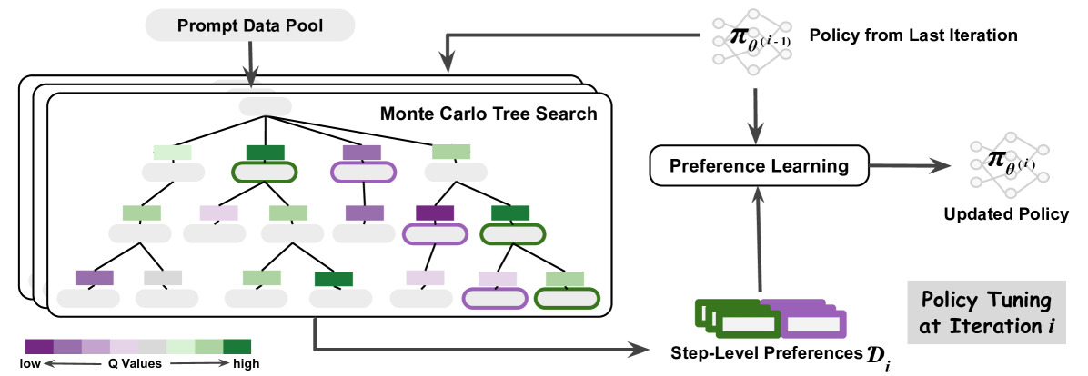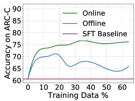</details> Figure 1: Monte Carlo Tree Search (MCTS) boosts model performance via iterative preference learning. Each iteration of our framework (on the left) consists of two stages: MCTS to collect step-level preferences and preference learning to update the policy. Specifically, we use action values $Q$ estimated by MCTS to assign the preferences, where steps of higher and lower $Q$ values will be labeled as positive and negative data, respectively. The scale of $Q$ is visualized in the colormap. We show the advantage of the online manner in our iterative learning framework using the validation accuracy curves as training progresses on the right. The performance of ARC-C validation illustrates the effectiveness and efficiency of our proposed method compared to its offline variant. A compelling illustration of the success of such an iterative approach can be seen in the case of AlphaZero (Silver et al., 2017) for its superhuman performance across various domains, which combines the strengths of neural networks, RL techniques, and Monte Carlo Tree Search (MCTS) (Coulom, 2006; Kocsis and Szepesvári, 2006). The integration of MCTS as a policy improvement operator that transforms the current policy into an improved policy (Grill et al., 2020). The effectiveness of AlphaZero underscores the potential of combining these advanced techniques in LLMs. By integrating MCTS into the iterative process of policy development, it is plausible to achieve significant strides in LLMs, particularly in the realm of reasoning and decision-making aligned with human-like preferences (Zhu et al., 2023; Hao et al., 2023). The integration of MCTS in collecting preference data to improve the current policy iteratively is nuanced and demands careful consideration. One primary challenge lies in determining the appropriate granularity for applying MCTS. Conventionally, preference data is collected at the instance level. The instance-level approach employs sparse supervision, which can lose important information and may not optimally leverage the potential of MCTS in improving the LLMs (Wu et al., 2023). Another challenge is the reliance of MCTS on a critic or a learned reward function. This function is crucial for providing meaningful feedback on different rollouts generated by MCTS, thus guiding the policy improvement process (Liu et al., 2023a). Addressing this granularity issue, evidence from LLM research indicates the superiority of process-level or stepwise evaluations over instance-level ones (Lightman et al., 2023; Li et al., 2023; Xie et al., 2023; Yao et al., 2023). Our approach utilizes MCTS rollouts for step-level guidance, aligning with a more granular application of MCTS. Moreover, we employ self-evaluation, where the model assesses its outputs, fostering a more efficient policy improvement pipeline by acting as both policy and critic (Kadavath et al., 2022; Xie et al., 2023). This method streamlines the process and ensures more cohesive policy updates, aligning with the iterative nature of policy enhancement and potentially leading to more robust and aligned LLMs. To summarize, we propose an algorithm based on Monte Carlo Tree Search (MCTS) that breaks down the instance-level preference signals into step-level. MCTS allows us to use the current LLM policy to generate preference data instead of a predetermined set of human preference data, enabling the LLM to receive real-time training signals. During training, we generate sequences of text on the fly and label the preference via MCTS based on feedback from self-evaluation (Figure 1). To update the LLM policy using the preference data, we use Direct Preference Optimization (DPO) (Rafailov et al., 2023). We extensively evaluate the proposed approach on various arithmetic and commonsense reasoning tasks and observe significant performance improvements. For instance, the proposed approach outperforms the Mistral-7B SFT baseline by $81.8\%$ (+ $5.9\%$ ), $34.7\%$ (+ $5.8\%$ ), and $76.4\%$ (+ $15.8\%$ ) on GSM8K, MATH, and SciQ, respectively. Further analysis of the training and test compute tradeoff shows that our method can effectively push the performance gains in a more efficient way compared to sampling-only approaches. 2 MCTS-Enhanced Iterative Preference Learning In this paper, we introduce an approach for improving LLM reasoning, centered around an iterative preference learning process. The proposed method begins with an initial policy $\pi_{\theta^{(0)}}$ , and a dataset of prompts $\mathcal{D}_{\mathcal{P}}$ . Each iteration $i$ involves selecting a batch of prompts from $\mathcal{D}_{\mathcal{P}}$ , from which the model, guided by its current policy $\pi_{\theta^{(i-1)}}$ , generates potential responses for each prompt. We then apply a set of dynamically evolving reward criteria to extract preference data $\mathcal{D}_{i}$ from these responses. The model’s policy is subsequently tuned using this preference data, leading to an updated policy $\pi_{\theta^{(i)}}$ , for the next iteration. This cycle of sampling, response generation, preference extraction, and policy tuning is repeated, allowing for continuous self-improvement and alignment with evolving preferences. In addressing the critical aspects of this methodology, two key challenges emerge: the effective collection of preference data and the process of updating the policy post-collection. We draw upon the concept that MCTS can act as an approximate policy improvement operator, transforming the current policy into an improved one. Our work leverages MCTS to iteratively collect preference data, utilizing its look-ahead ability to break down instance-level rewards into more granular step-level signals. To enhance consistency in intermediate steps, we incorporate stepwise self-evaluation, continually updating the quality assessment of newly generated data. This process, as depicted in Figure 1, enables MCTS to balance quality exploitation and diversity exploration during preference data sampling at each iteration. Detailed in section 2.1, our approach utilizes MCTS for step-level preference data collection. Once this data is collected, the policy is updated using DPO, as outlined in section 2.2. Our method can be viewed as an online version of DPO, where the updated policy is iteratively employed to collect preferences via MCTS. Our methodology, thus, not only addresses the challenges in preference data collection and policy updating but also introduces a dynamic, iterative framework that significantly enhances LLM reasoning. {algorithm*} [tb] . MCTS-Enhanced Iterative Preference Learning. Given an initial policy $\pi_{\theta^{(0)}}=\pi_{\mathrm{sft}}$ , our algorithm iteratively conducts step-level preference data sampling via MCTS and preference learning via DPO to update the policy. {algorithmic} \STATE Input: $\mathcal{D}_{\mathcal{P}}$ : prompt dataset; $q(·\mid x)$ : MCTS sampling strategy that constructs a tree-structured set of possible responses given a prompt $x$ , where $q_{\pi}$ represents that the strategy is based on the policy $\pi$ for both response generation and self-evaluation; $\ell_{i}(x,y_{w},y_{l};\theta)$ : loss function of preference learning at the $i$ -th iteration, where the corresponding sampling policy is $\pi^{(i)}$ ; $M$ : number of iterations; $B$ : number of samples per iteration; $T$ : average number of steps per sample \STATE Train $\pi_{\theta}$ on $\mathcal{D}_{\mathcal{P}}$ using step-level preference learning. \FOR $i=1$ to $M$ \STATE $\pi^{(i)}←\pi_{\theta}←\pi_{\theta^{(i-1)}}$ \STATE Sample a batch of $B$ samples from $\mathcal{D}_{\mathcal{P}}$ as $\mathcal{D}_{\mathcal{P}}^{(i)}$ . \STATE \COMMENT MCTS for Step-Level Preference Data Collection \STATE For each $x∈\mathcal{D}_{\mathcal{P}}^{(i)}$ , elicit a search tree of depth $T$ via $q_{\pi_{\theta}}(·\mid x)$ . \STATE Collect a batch of preferences $\mathcal{D}_{i}=\{$ $\{(x^{j},y_{l}^{(j,t)},y_{l}^{(j,t)})|_{t=1}^{T}\}|_{j=1}^{B}$ s.t. $x^{j}\sim\mathcal{D}_{\mathcal{P}}^{(i)},y_{w}^{(j,t)}≠ y_{w}^{(j,t)}\sim q% _{\pi_{\theta}}(·\mid x^{j})$ $\}$ , where $y_{w}^{(j,t)}$ and $y_{l}^{(j,t)}$ is the nodes at depth $t$ , with the highest and lowest $Q$ values, respectively, among all the children nodes of their parent node. \STATE \COMMENT Preference Learning for Policy Improvement \STATE Optimize $\theta$ by minimizing $J(\theta)=\mathbb{E}_{(x,y_{w},y_{l})\sim\mathcal{D}_{i}}\ell_{i}(x,y_{w},y_{l% };\theta)$ . \STATE Obtain the updated policy $\pi_{\theta^{(i)}}$ \ENDFOR \STATE $\pi_{\theta}←\pi_{\theta^{(M)}}$ \STATE Output: Policy $\pi_{\theta}$ 2.1 MCTS for Step-Level Preference To transform instance-level rewards into granular, step-level signals, we dissect the reasoning process into discrete steps, each represented by a token sequence. We define the state at step $t$ , $s_{t}$ , as the prefix of the reasoning chain, with the addition of a new reasoning step $a$ transitioning the state to $s_{t+1}$ , where $s_{t+1}$ is the concatenation of $s_{t}$ and $a$ . Utilizing the model’s current policy $\pi_{\theta}$ , we sample candidate steps from its probability distribution $\pi_{\theta}(a\mid x,s_{t})$ For tasks (e.g., MATH) where the initial policy performs poorly, we also include the ground-truth reasoning steps for training. We detail the step definition for different tasks with examples in Appendices C and D., with $x$ being the task’s input prompt. MCTS serves as an approximate policy improvement operator by leveraging its look-ahead capability to predict the expected future reward. This prediction is refined through stepwise self-evaluation (Kadavath et al., 2022; Xie et al., 2023), enhancing process consistency and decision accuracy. The tree-structured search supports a balance between exploring diverse possibilities and exploiting promising paths, essential for navigating the vast search space in LLM reasoning. The MCTS process begins from a root node, $s_{0}$ , as the sentence start or incomplete response, and unfolds in three iterative stages: selection, expansion, and backup, which we detail further. Select. The objective of this phase is to identify nodes that balance search quality and computational efficiency. The selection is guided by two key variables: $Q(s_{t},a)$ , the value of taking action $a$ in state $s_{t}$ , and $N(s_{t})$ , the visitation frequency of state $s_{t}$ . These variables are crucial for updating the search strategy, as explained in the backup section. To navigate the trade-off between exploring new nodes and exploiting visited ones, we employ the Predictor + Upper Confidence bounds applied to Trees (PUCT) (Rosin, 2011). At node $s_{t}$ , the choice of the subsequent node follows the formula: $$ \displaystyle{s_{t+1}}^{*} \displaystyle=\arg\max_{s_{t}}\Bigl{[}Q(s_{t},a)+c_{\mathrm{puct}}\cdot p(a% \mid s_{t})\frac{\sqrt{N(s_{t})}}{1+N(s_{t+1})}\Bigl{]} \tag{1} $$ where $p(a\mid s_{t})=\pi_{\theta}(a\mid x,s_{t})/|a|^{\lambda}$ denotes the policy $\pi_{\theta}$ ’s probability distribution for generating a step $a$ , adjusted by a $\lambda$ -weighted length penalty to prevent overly long reasoning chains. Expand. Expansion occurs at a leaf node during the selection process to integrate new nodes and assess rewards. The reward $r(s_{t},a)$ for executing step $a$ in state $s_{t}$ is quantified by the reward difference between states $R(s_{t})$ and $R(s_{t+1})$ , highlighting the advantage of action $a$ at $s_{t}$ . As defined in Eq. (2), reward computation merges outcome correctness $\mathcal{O}$ with self-evaluation $\mathcal{C}$ . We assign the outcome correctness to be $1$ , $-1$ , and $0 0$ for correct terminal, incorrect terminal, and unfinished intermediate states, respectively. Following Xie et al. (2023), we define self-evaluation as Eq. (3), where $\mathrm{A}$ denotes the confidence score in token-level probability for the option indicating correctness We show an example of evaluation prompt in Table 6.. Future rewards are anticipated by simulating upcoming scenarios through roll-outs, following the selection and expansion process until reaching a terminal state The terminal state is reached when the whole response is complete or exceeds the maximum length.. $$ R(s_{t})=\mathcal{O}(s_{t})+\mathcal{C}(s_{t}) \tag{2} $$ $$ \mathcal{C}(s_{t})=\pi_{\theta}(\mathrm{A}\mid{\mathrm{prompt}}_{\mathrm{eval}% },x,s_{t}) \tag{3} $$ Backup. Once a terminal state is reached, we carry out a bottom-up update from the terminal node back to the root. We update the visit count $N$ , the state value $V$ , and the transition value $Q$ : $$ Q(s_{t},a)\leftarrow r(s_{t},a)+\gamma V(s_{t+1}) \tag{4} $$ $$ V(s_{t})\leftarrow\sum_{a}N(s_{t+1})Q(s_{t},a)/\sum_{a}N(s_{t+1}) \tag{5} $$ $$ N(s_{t})\leftarrow N(s_{t})+1 \tag{6} $$ where $\gamma$ is the discount for future state values. For each step in the response generation, we conduct $K$ iterations of MCTS to construct the search tree while updating $Q$ values and visit counts $N$ . To balance the diversity, quality, and efficiency of the tree construction, we initialize the search breadth as $b_{1}$ and anneal it to be a smaller $b_{2}<b_{1}$ for the subsequent steps. We use the result $Q$ value corresponding to each candidate step to label its preference, where higher $Q$ values indicate preferred next steps. For a result search tree of depth $T$ , we obtain $T$ pairs of step-level preference data. Specifically, we select the candidate steps of highest and lowest $Q$ values as positive and negative samples at each tree depth, respectively. The parent node selected at each tree depth has the highest value calculated by multiplying its visit count and the range of its children nodes’ visit counts, indicating both the quality and diversity of the generations. 2.2 Iterative Preference Learning Given the step-level preferences collected via MCTS, we tune the policy via DPO (Rafailov et al., 2023). Considering the noise in the preference labels determined by $Q$ values, we employ the conservative version of DPO (Mitchell, 2023) and use the visit counts simulated in MCTS to apply adaptive label smoothing on each preference pair. Using the shorthand $h_{\pi_{\theta}}^{y_{w},y_{l}}=\log\frac{\pi_{\theta}(y_{w}\mid x)}{\pi_{% \mathrm{ref}}(y_{w}\mid x)}-\log\frac{\pi_{\theta}(y_{l}\mid x)}{\pi_{\mathrm{% ref}}(y_{l}\mid x)}$ , at the $i$ -th iteration, given a batch of preference data $\mathcal{D}_{i}$ sampled with the latest policy $\pi_{\theta^{(i-1)}}$ , we denote the policy objective $\ell_{i}(\theta)$ as follows: $$ \displaystyle\ell_{i}(\theta)= \displaystyle-\mathbb{E}_{(x,y_{w},y_{l})\sim\mathcal{D}_{i}}\Bigr{[}(1-\alpha% _{x,y_{w},y_{l}})\log\sigma(\beta\left.h_{\pi_{\theta}}^{y_{w},y_{l}}\right)+ \displaystyle\alpha_{x,y_{w},y_{l}}\log\sigma(-\beta h_{\pi_{\theta}}^{y_{w},y% _{l}})\Bigr{]} \tag{7} $$ where $y_{w}$ and $y_{l}$ represent the step-level preferred and dispreferred responses, respectively, and the hyperparameter $\beta$ scales the KL constraint. Here, $\alpha_{x,y_{w},y_{l}}$ is a label smoothing variable calculated using the visit counts at the corresponding states of the preference data $y_{w}$ , $y_{l}$ in the search tree: $$ \alpha_{x,y_{w},y_{l}}=\frac{1}{N(x,y_{w})/N(x,y_{l})+1} \tag{8} $$ where $N(x,y_{w})$ and $N(x,y_{l})$ represent the states taking the actions of generating $y_{w}$ and $y_{l}$ , respectively, from their previous state as input $x$ . After optimization, we obtain the updated policy $\pi_{\theta^{(i)}}$ and repeat the data collection process in Section 2.1 to iteratively update the LLM policy. We outline the full algorithm of our MCTS-enhanced Iterative Preference Learning in Algorithm 2. 3 Theoretical Analysis Our approach can be viewed as an online version of DPO, where we iteratively use the updated policy to sample preferences via MCTS. In this section, we provide theoretical analysis to interpret the advantages of our online learning framework compared to the conventional alignment techniques that critically depend on offline preference data. We review the typical RLHF and DPO paradigms in Appendix B. We now consider the following abstract formulation for clean theoretical insights to analyze our online setting of preference learning. Given a prompt $x$ , there exist $n$ possible suboptimal responses $\{\bar{y}_{1},...,\bar{y}_{n}\}=Y$ and an optimal outcome $y^{*}$ . As specified in Equation 7, at the $i$ -th iteration, a pair of responses $(y,{y^{\prime}})$ are sampled from some sampling policy $\pi^{(i)}$ without replacement so that $y≠{y^{\prime}}$ as $y\sim\pi^{(i)}(·\mid x)$ and ${y^{\prime}}\sim\pi^{(i)}(·\mid x,y)$ . Then, these are labeled to be $y_{w}$ and $y_{l}$ according to the preference. Define $\Theta$ be a set of all global optimizers of the preference loss for all $M$ iterations, i.e., for any $\theta∈\Theta$ , $\ell_{i}(\theta)=0$ for all $i∈\{1,2,·s,M\}$ . Similarly, let ${\theta^{(i)}}$ be a parameter vector such that $\ell_{j}(\theta^{(i)})=0$ for all $j∈\{1,2,·s,i-1\}$ for $i≥ 1$ whereas $\theta^{(0)}$ is the initial parameter vector. This abstract formulation covers both the offline and online settings. The offline setting in previous works is obtained by setting $\pi^{(i)}=\pi$ for some fixed distribution $\pi$ . The online setting is obtained by setting $\pi^{(i)}=\pi_{\theta^{(i-1)}}$ where $\pi_{\theta^{(i-1)}}$ is the latest policy at beginning of the $i$ -th iteration. The following theorem shows that the offline setting can fail with high probability if the sampling policy $\pi^{(i)}$ differs too much from the current policy $\pi_{\theta^{(i-1)}}$ : **Theorem 3.1 (Offline setting can fail with high probability)** *Let $\pi$ be any distribution for which there exists $\bar{y}∈ Y$ such that $\pi(\bar{y}\mid x),\pi(\bar{y}\mid x,y)≤\epsilon$ for all $y∈(Y\setminus\bar{y})\cup\{y^{*}\}$ and $\pi_{\theta^{(i-1)}}(\bar{y}\mid x)≥ c$ for some $i∈\{1,2,·s,M\}$ . Set $\pi^{(i)}=\pi$ for all $i∈\{1,2,·s,M\}$ . Then, there exists $\theta∈\Theta$ such that with probability at least $1-2\epsilon M$ (over the samples of $\pi^{(i)}=\pi$ ), the following holds: $\pi_{\theta}(y^{*}\mid x)≤ 1-c$ .* If the current policy and the sampling policy differ too much, it is possible that $\epsilon=0$ and $c≈ 1.0$ , for which Theorem 3.1 can conclude $\pi_{\theta}(y^{*}\mid x)≈ 0$ with probability $1$ for any number of steps $M$ . When $\epsilon≠ 0$ , the lower bound of the failure probability decreases towards zero as we increase $M$ . Thus, it is important to make sure that $\epsilon≠ 0$ and $\epsilon$ is not too low. This is achieved by using the online setting, i.e., $\pi^{(i)}=\pi_{\theta^{(i)}}$ . Therefore, Theorem 3.1 motivates us to use the online setting. Theorem 3.2 confirms that we can indeed avoid this failure case in the online setting. **Theorem 3.2 (Online setting can avoid offline failure case)** *Let $\pi^{(i)}=\pi_{\theta^{(i-1)}}$ . Then, for any $\theta∈\Theta$ , it holds that $\pi_{\theta}(y^{*}\mid x)=1$ if $M≥ n+1$ .* See Appendix B for the proofs of Theorems 3.1 and 3.2. As suggested by the theorems, a better sampling policy is to use both the latest policy and the optimal policy for preference sampling. However, since we cannot access the optimal policy $\pi^{*}$ in practice, we adopt online DPO via sampling from the latest policy $\pi_{\theta^{(i-1)}}$ . The key insight of our iterative preference learning approach is that online DPO is proven to enable us to converge to an optimal policy even if it is inaccessible to sample outputs. We provide further discussion and additional insights in Appendix B. 4 Experiments We evaluate the effectiveness of MCTS-enhanced iterative preference learning on arithmetic and commonsense reasoning tasks. We employ Mistral-7B (Jiang et al., 2023) as the base pre-trained model. We conduct supervised training using Arithmo https://huggingface.co/datasets/akjindal53244/Arithmo-Data which comprises approximately $540$ K mathematical and coding problems. Detailed information regarding the task formats, specific implementation procedures, and parameter settings of our experiments can be found in Appendix C. Datasets. We aim to demonstrate the effectiveness and versatility of our approach by focusing on two types of reasoning: arithmetic and commonsense reasoning. For arithmetic reasoning, we utilize two datasets: GSM8K (Cobbe et al., 2021), which consists of grade school math word problems, and MATH (Hendrycks et al., 2021), featuring challenging competition math problems. Specifically, in the GSM8K dataset, we assess both chain-of-thought (CoT) and program-of-thought (PoT) reasoning abilities. We integrate the training data from GSM8K and MATH to construct the prompt data for our preference learning framework, aligning with a subset of the Arithmo data used for Supervised Fine-Tuning (SFT). This approach allows us to evaluate whether our method enhances reasoning abilities on specific arithmetic tasks. For commonsense reasoning, we use four multiple-choice datasets: ARC (easy and challenge splits) (Clark et al., 2018), focusing on science exams; AI2Science (elementary and middle splits) (Clark et al., 2018), containing science questions from student assessments; OpenBookQA (OBQA) (Mihaylov et al., 2018), which involves open book exams requiring broad common knowledge; and CommonSenseQA (CSQA) (Talmor et al., 2019), featuring commonsense questions necessitating prior world knowledge. The diversity of these datasets, with different splits representing various grade levels, enables a comprehensive assessment of our method’s generalizability in learning various reasoning tasks through self-distillation. Performance evaluation is conducted using the corresponding validation sets of each dataset. Furthermore, we employ an unseen evaluation using the validation set of an additional dataset, SciQ (Welbl et al., 2017), following the approach of Liu et al. (2023b), to test our model’s ability to generalize to novel reasoning contexts. Baselines. Our study involves a comparative evaluation of our method against several prominent approaches and fair comparison against variants including instance-level iterative preference learning and offline MCTS-enhanced learning. We use instance-level sampling as a counterpart of step-level preference collection via MCTS. For a fair comparison, we also apply self-evaluation and correctness assessment and control the number of samples under a comparable compute budget with MCTS in instance-level sampling. The offline version uses the initial policy for sampling rather than the updated one at each iteration. We contrast our approach with the Self-Taught Reasoner (STaR) (Zelikman et al., 2022), an iterated learning model based on instance-level rationale generation, and Crystal (Liu et al., 2023b), an RL-tuned model with a focus on knowledge introspection in commonsense reasoning. Considering the variation in base models used by these methods, we include comparisons with Direct Tuning, which entails fine-tuning base models directly bypassing chain-of-thought reasoning. In the context of arithmetic reasoning tasks, our analysis includes Language Model Self-Improvement (LMSI) (Huang et al., 2023), a self-training method using self-consistency to gather positive data, and Math-Shepherd (Wang et al., 2023a), which integrates process supervision within Proximal Policy Optimization (PPO). To account for differences in base models and experimental setups across these methods, we also present result performance of SFT models as baselines for each respective approach. Table 1: Result comparison (accuracy $\%$ ) on arithmetic tasks. We supervised fine-tune the base model Mistral-7B on Arithmo data, while Math-Shepherd (Wang et al., 2023a) use MetaMATH (Yu et al., 2023b) for SFT. We highlight the advantages of our approach via conceptual comparison with other methods, where NR, OG, OF, and NS represent “w/o Reward Model”, “On-policy Generation”, “Online Feedback”, and “w/ Negative Samples”. | Approach | Base Model | Conceptual Comparison | GSM8K | MATH | | | | | --- | --- | --- | --- | --- | --- | --- | --- | | NR | OG | OF | NS | | | | | | LMSI | PaLM-540B | ✓ | ✓ | ✗ | ✗ | $73.5$ | $-$ | | SFT (MetaMath) | Mistral-7B | $-$ | $-$ | $-$ | $-$ | $77.7$ | $28.2$ | | Math-Shepherd | ✗ | ✓ | ✗ | ✓ | $\mathbf{84.1}$ | $33.0$ | | | SFT (Arithmo) | Mistral-7B | $-$ | $-$ | $-$ | $-$ | $75.9$ | $28.9$ | | MCTS Offline-DPO | ✓ | ✗ | ✗ | ✓ | $79.9$ | $31.9$ | | | Instance-level Online-DPO | ✓ | ✓ | ✓ | ✓ | $79.7$ | $32.9$ | | | Ours | ✓ | ✓ | ✓ | ✓ | $80.7$ | $32.2$ | | | Ours (w/ G.T.) | | ✓ | ✓ | ✓ | ✓ | $81.8$ | $\mathbf{34.7}$ | <details> <summary>x3.png Details</summary>  ### Visual Description ## Line Chart: ARC-C Accuracy vs Training Data Percentage ### Overview The chart compares the accuracy of four different training approaches (Step-Level Online, Instance-Level Online, Step-Level Offline, and SFT Baseline) across varying percentages of training data (10-50%). Accuracy is measured on the y-axis (55-75), while training data percentage is on the x-axis (10-50%). ### Components/Axes - **X-axis**: Training Data % (10, 20, 30, 40, 50) - **Y-axis**: Accuracy (55-75, increments of 5) - **Legend**: Located at bottom-left, with four entries: - Green line with stars: Step-Level (Online) - Blue line with triangles: Instance-Level (Online) - Yellow line with stars: Step-Level (Offline) - Purple dashed line: SFT Baseline - **Title**: "ARC-C" at top-center ### Detailed Analysis 1. **Step-Level (Online)** (Green): - Starts at 72.2% accuracy at 10% training data - Peaks at 76.4% at 30% training data - Slight decline to 75.8% at 50% training data - Trend: Initial sharp increase followed by stabilization 2. **Instance-Level (Online)** (Blue): - Begins at 66.5% at 10% training data - Rises to 73.3% at 30% training data - Peaks at 75.2% at 40% training data - Drops to 73.4% at 50% training data - Trend: Gradual improvement then decline 3. **Step-Level (Offline)** (Yellow): - Starts at 69.2% at 10% training data - Peaks at 70.8% at 20% training data - Declines to 66.5% at 50% training data - Trend: Early peak followed by steady decline 4. **SFT Baseline** (Purple dashed): - Constant at 60.6% across all training data percentages - Trend: Flat line with no variation ### Key Observations - Step-Level (Online) consistently outperforms all other methods - Instance-Level (Online) shows the most significant improvement between 10% and 40% training data - Step-Level (Offline) underperforms compared to its online counterpart - SFT Baseline remains the lowest-performing method throughout - All methods show diminishing returns beyond 30-40% training data ### Interpretation The data demonstrates that online training approaches (both step-level and instance-level) significantly outperform offline methods and the SFT baseline. The Step-Level (Online) method achieves the highest accuracy (76.4%) at 30% training data, suggesting optimal performance at this threshold. The Instance-Level (Online) method shows the most dramatic improvement (from 66.5% to 75.2%) as training data increases, indicating strong scalability. The consistent decline in Step-Level (Offline) performance highlights the importance of online training dynamics. The flat SFT Baseline suggests it represents a fundamental lower bound for this particular task. The diminishing returns observed across all methods beyond 40% training data implies potential inefficiencies in utilizing larger datasets without proportional accuracy gains. 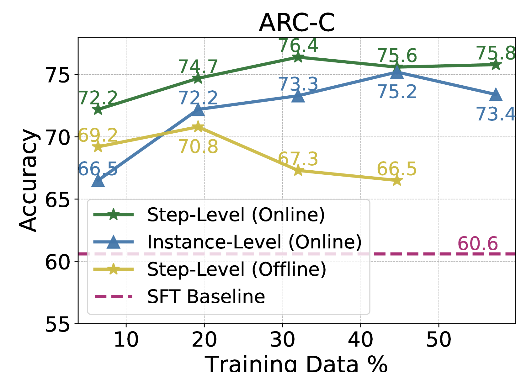</details> Figure 2: Performance on the validation set of ARC-C via training with different settings. Table 2: Result comparisons (accuracy $\%$ ) on commonsense reasoning tasks. The results based on GPT-3-curie (Brown et al., 2020) and T5 (Raffel et al., 2020) are reported from Liu et al. (2023b). For CSQA, we also include the GPT-J (Wang and Komatsuzaki, 2021) results reported by Zelikman et al. (2022). We follow Liu et al. (2023b) to combine the training data of ARC, AI2Sci, OBQA, and CSQA for training , while STaR (Zelikman et al., 2022) only use CSQA for training. | Approach | Base Model | Conceptual Comparison | ARC-c | AI2Sci-m | CSQA | SciQ | Train Data Used ( $\%$ ) | | | | | --- | --- | --- | --- | --- | --- | --- | --- | --- | --- | --- | | NR | OG | OF | NS | | | | | | | | | CoT Tuning | GPT-3-curie (6.7B) | ✓ | ✗ | ✗ | ✗ | $-$ | $-$ | $56.8$ | $-$ | $100$ | | Direct Tuning | GPT-J (6B) | ✓ | ✗ | ✗ | ✗ | $-$ | $-$ | $60.0$ | $-$ | $100$ | | STaR | ✓ | ✓ | ✓ | ✗ | $-$ | $-$ | $72.5$ | $-$ | $86.7$ | | | Direct TUning | T5-11B | ✓ | ✗ | ✗ | ✗ | $72.9$ | $84.0$ | $82.0$ | $83.2$ | $100$ | | Crystal | ✗ | ✓ | ✓ | ✓ | $73.2$ | $84.8$ | $\mathbf{82.3}$ | $85.3$ | $100$ | | | SFT Base (Arithmo) | Mistral-7B | $-$ | $-$ | $-$ | $-$ | $60.6$ | $70.9$ | $54.1$ | $80.8$ | $-$ | | Direct Tuning | ✓ | ✗ | ✗ | ✗ | $73.9$ | $85.2$ | $79.3$ | $86.4$ | $100$ | | | MCTS Offline-DPO | ✓ | ✗ | ✗ | ✓ | $70.8$ | $82.6$ | $68.5$ | $87.4$ | $19.2$ | | | Instance-level Online-DPO | ✓ | ✓ | ✓ | ✓ | $75.3$ | $87.3$ | $63.1$ | $87.6$ | $45.6$ | | | Ours | ✓ | ✓ | ✓ | ✓ | $\mathbf{76.4}$ | $\mathbf{88.2}$ | $74.8$ | $\mathbf{88.5}$ | $47.8$ | | 4.1 Main Results Arithmetic Reasoning. In Table 1, we present a comparative analysis of performance gains in arithmetic reasoning tasks. Our method demonstrates substantial improvements, notably on GSM8K, increasing from $75.9\%→ 81.8\%$ , and on MATH, enhancing from $28.9\%→ 34.7\%$ . When compared to Math-Shepherd, which also utilizes process supervision in preference learning, our approach achieves similar performance enhancements without the necessity of training separate reward or value networks. This suggests the potential of integrating trained reward model signals into our MCTS stage to further augment performance. Furthermore, we observe significant performance gain on MATH when incorporating the ground-truth solutions in the MCTS process for preference data collection, illustrating an effective way to refine the preference data quality with G.T. guidance. <details> <summary>x4.png Details</summary>  ### Visual Description ## Line Charts: ARC-C Performance and Accuracy Metrics ### Overview The image contains two line charts comparing performance metrics across different training approaches. The top chart ("ARC-C") tracks pass rates against checkpoint progression, while the bottom chart ("Accuracy") measures accuracy against sampling iterations. Both include baseline comparisons and show distinct performance trajectories. ### Components/Axes **Top Chart (ARC-C):** - **Y-axis**: Pass Rate (60-95) - **X-axis**: # Checkpoints (0-7) - **Legend**: - Green triangles: Iterative Learning (Pass@1) - Green stars: Iterative Learning (Cumulative) - Blue stars: Sampling Only (Cumulative) - Red dashed line: SFT Baseline (Pass@1) **Bottom Chart (Accuracy):** - **Y-axis**: Accuracy (60-95) - **X-axis**: k (10-60) - **Legend**: - Blue triangles: Sampling Only (SC@k) - Red dashed line: SFT Baseline (Pass@1) ### Detailed Analysis **ARC-C Chart Data Points:** - **Iterative Learning (Pass@1)**: - 0: 60.6 → 1: 79.7 → 2: 86.9 → 3: 90.0 → 4: 91.3 → 5: 92.4 → 6: 93.3 → 7: 94.1 - **Iterative Learning (Cumulative)**: - 0: 60.6 → 1: 72.2 → 2: 73.6 → 3: 74.7 → 4: 75.1 → 5: 76.4 → 6: 75.8 → 7: 76.2 - **Sampling Only (Cumulative)**: - 0: 60.6 → 1: 71.9 → 2: 80.6 → 3: 86.6 → 4: 89.3 → 5: 91.7 → 6: 92.9 → 7: 93.5 - **SFT Baseline**: Constant 60.6 across all checkpoints **Accuracy Chart Data Points:** - **Sampling Only (SC@k)**: - k=10: 61.9 → k=20: 72.2 → k=30: 73.4 → k=60: 74.1 - **SFT Baseline**: Constant 60.6 across all k values ### Key Observations 1. **ARC-C Performance**: - Iterative Learning (Pass@1) shows exponential growth, reaching 94.1 at 7 checkpoints - Cumulative metrics plateau earlier (76.2 at 7 checkpoints) vs Pass@1 - Sampling Only closes the gap significantly by checkpoint 7 (93.5 vs 94.1) - SFT Baseline remains static at 60.6, indicating poor scalability 2. **Accuracy Trends**: - Sampling Only improves gradually (61.9 → 74.1) with increasing k - SFT Baseline shows no improvement despite increased sampling - Sampling Only achieves 13.5 accuracy point improvement over baseline ### Interpretation The data demonstrates that iterative learning methods outperform static SFT baselines, with cumulative approaches showing diminishing returns after initial checkpoints. Sampling-based methods (both iterative and standalone) achieve near-parity with iterative learning by checkpoint 7, suggesting sampling efficiency improves with scale. The SFT baseline's stagnation across both metrics indicates fundamental limitations in static training approaches for complex tasks requiring iterative refinement. The convergence of Sampling Only and Iterative Learning metrics at higher checkpoints implies that sampling strategies may effectively approximate iterative learning benefits at scale. </details> <details> <summary>x5.png Details</summary>  ### Visual Description ## Line Graphs: SciQ and SC@k Performance Comparison ### Overview The image contains two line graphs comparing performance metrics across different training methods. The top graph ("SciQ") tracks performance against the number of checkpoints, while the bottom graph ("SC@k") evaluates performance against the number of samples (k). Both graphs use percentage scores on the y-axis and numerical values on the x-axis. --- ### Components/Axes #### SciQ Graph - **X-axis**: "# Checkpoints" (0–7, integer increments) - **Y-axis**: Percentage (%) (80–100, 2.5% increments) - **Legend**: - Green triangles: Iterative Learning (Pass@1) - Green stars: Iterative Learning (Cumulative) - Blue stars: Sampling Only (Cumulative) - Dashed purple line: SFT Baseline (Pass@1) - **Legend Position**: Top-left corner #### SC@k Graph - **X-axis**: "k" (10–60, integer increments) - **Y-axis**: Percentage (%) (80–100, 2.5% increments) - **Legend**: - Blue triangles: Sampling Only (SC@k) - Dashed purple line: SFT Baseline (Pass@1) - **Legend Position**: Top-right corner --- ### Detailed Analysis #### SciQ Graph - **Iterative Learning (Pass@1)**: - Starts at 80.8% (checkpoint 0) and rises to 96.3% (checkpoint 7). - Key values: 89.6% (1), 86.0% (2), 88.3% (3), 86.5% (4), 88.5% (5), 87.7% (6), 96.3% (7). - **Trend**: Steady upward trajectory with minor fluctuations. - **Iterative Learning (Cumulative)**: - Starts at 91.2% (checkpoint 1) and increases to 95.9% (checkpoint 6). - Key values: 91.2% (1), 93.9% (2), 95.9% (6). - **Trend**: Gradual upward slope. - **Sampling Only (Cumulative)**: - Starts at 82.8% (checkpoint 1) and rises to 91.5% (checkpoint 7). - Key values: 82.8% (1), 86.4% (3), 89.8% (5), 91.5% (7). - **Trend**: Consistent upward slope. - **SFT Baseline (Pass@1)**: - Flat line at 80.8% across all checkpoints. #### SC@k Graph - **Sampling Only (SC@k)**: - Starts at 81.6% (k=10) and increases to 84.4% (k=60). - Key values: 82.8% (k=15), 83.8% (k=20), 84.1% (k=25), 84.2% (k=35), 84.4% (k=60). - **Trend**: Slight upward slope with diminishing returns. - **SFT Baseline (Pass@1)**: - Flat line at 80.8% across all k values. --- ### Key Observations 1. **SciQ Graph**: - Iterative Learning (Cumulative) outperforms all methods, reaching 95.9% at checkpoint 6. - Sampling Only (Cumulative) shows the steepest improvement among non-iterative methods. - SFT Baseline remains stagnant at 80.8%, indicating no improvement with checkpoints. 2. **SC@k Graph**: - Sampling Only (SC@k) improves marginally with increased k (81.6% → 84.4%). - SFT Baseline remains unchanged, suggesting no benefit from scaling k. --- ### Interpretation - **Iterative Learning Dominance**: The SciQ graph demonstrates that iterative learning methods (especially cumulative approaches) significantly outperform sampling-only and baseline methods. This suggests that iterative refinement of checkpoints is critical for high performance. - **Diminishing Returns in Sampling**: The SC@k graph shows that increasing the number of samples (k) yields only modest gains for Sampling Only, implying that iterative strategies are more efficient than brute-force sampling. - **SFT Baseline Limitation**: The flat performance of the SFT Baseline across both graphs highlights its inability to adapt to incremental improvements, positioning it as a static reference point. - **Checkpoint vs. Sample Tradeoff**: While checkpoints drive substantial gains in SciQ, scaling samples (k) in SC@k has limited impact, emphasizing the importance of iterative training over static sampling. The data underscores the superiority of iterative learning frameworks in dynamic evaluation settings, while sampling-only approaches offer incremental but less impactful improvements. </details> <details> <summary>x6.png Details</summary>  ### Visual Description ## Line Graphs: Performance Comparison of Learning Methods ### Overview The image contains two line graphs comparing the performance of different learning methods across checkpoints. The top graph measures "Pass Rate" for math tasks, while the bottom graph measures "Accuracy" for sampling-based methods. Both graphs include a static SFT Baseline for comparison. ### Components/Axes **Top Graph (MATH Performance):** - **X-axis**: "# Checkpoints" (0 to 10) - **Y-axis**: "Pass Rate" (29 to 65) - **Legend**: - Green line with triangles: Iterative Learning (Pass@1) - Blue line with stars: Sampling Only (Cumulative) - Dashed red line: SFT Baseline (Pass@1) **Bottom Graph (Accuracy):** - **X-axis**: "k" (4 to 10) - **Y-axis**: "Accuracy" (29 to 65) - **Legend**: - Blue line with triangles: Sampling Only (SC@k) - Dashed red line: SFT Baseline (Pass@1) ### Detailed Analysis **Top Graph Trends:** 1. **Iterative Learning (Pass@1)**: - Starts at 29.0 (checkpoint 0) - Increases steadily to 57.1 (checkpoint 10) - Key milestones: 38.4 (checkpoint 2), 46.7 (checkpoint 4), 51.6 (checkpoint 6) 2. **Sampling Only (Cumulative)**: - Starts at 29.2 (checkpoint 0) - Outperforms Iterative Learning throughout - Reaches 57.9 (checkpoint 10) - Key milestones: 34.9 (checkpoint 2), 42.4 (checkpoint 4), 49.6 (checkpoint 6) 3. **SFT Baseline**: - Constant at 29.0 across all checkpoints **Bottom Graph Trends:** 1. **Sampling Only (SC@k)**: - Starts at 30.0 (k=4) - Gradual increase to 35.1 (k=10) - Key milestones: 31.5 (k=5), 32.2 (k=6), 33.3 (k=7), 34.2 (k=8) 2. **SFT Baseline**: - Constant at 29.0 across all k values ### Key Observations 1. **Performance Gains**: - Both Iterative Learning and Sampling Only show significant improvement over SFT Baseline - Sampling Only achieves higher pass rates than Iterative Learning in the top graph - Sampling Only's accuracy gains are modest but consistent 2. **Convergence**: - At checkpoint 10, Iterative Learning (57.1) and Sampling Only (57.9) are nearly identical in pass rate - Sampling Only maintains a slight accuracy advantage (35.1 vs. 29.0) 3. **Diminishing Returns**: - Top graph shows slowing improvement rates after checkpoint 6 - Bottom graph shows linear but minimal accuracy gains ### Interpretation The data demonstrates that both Iterative Learning and Sampling Only outperform the static SFT Baseline, with Sampling Only showing marginally better results in pass rate metrics. The cumulative nature of Sampling Only's approach appears more effective for math task performance, though both methods converge at higher checkpoint counts. The accuracy graph suggests Sampling Only's benefits manifest more gradually, with only a 5.1-point improvement across 6 additional checkpoints (k=4 to k=10). This implies that while Sampling Only provides consistent gains, the marginal returns per checkpoint decrease over time. The SFT Baseline's stagnation highlights the value of dynamic learning approaches in this context. 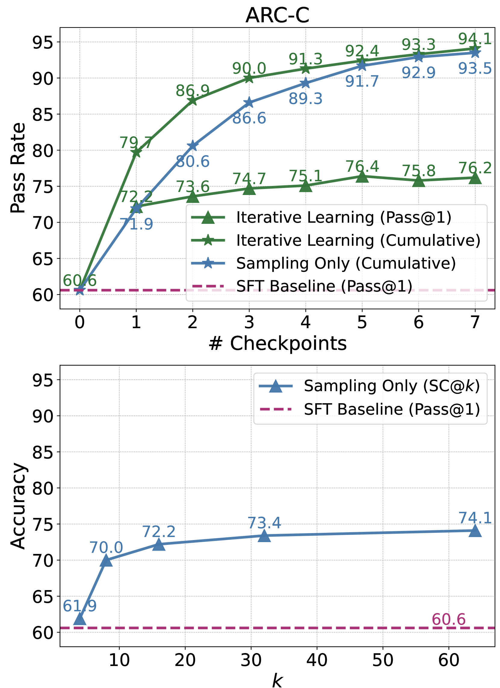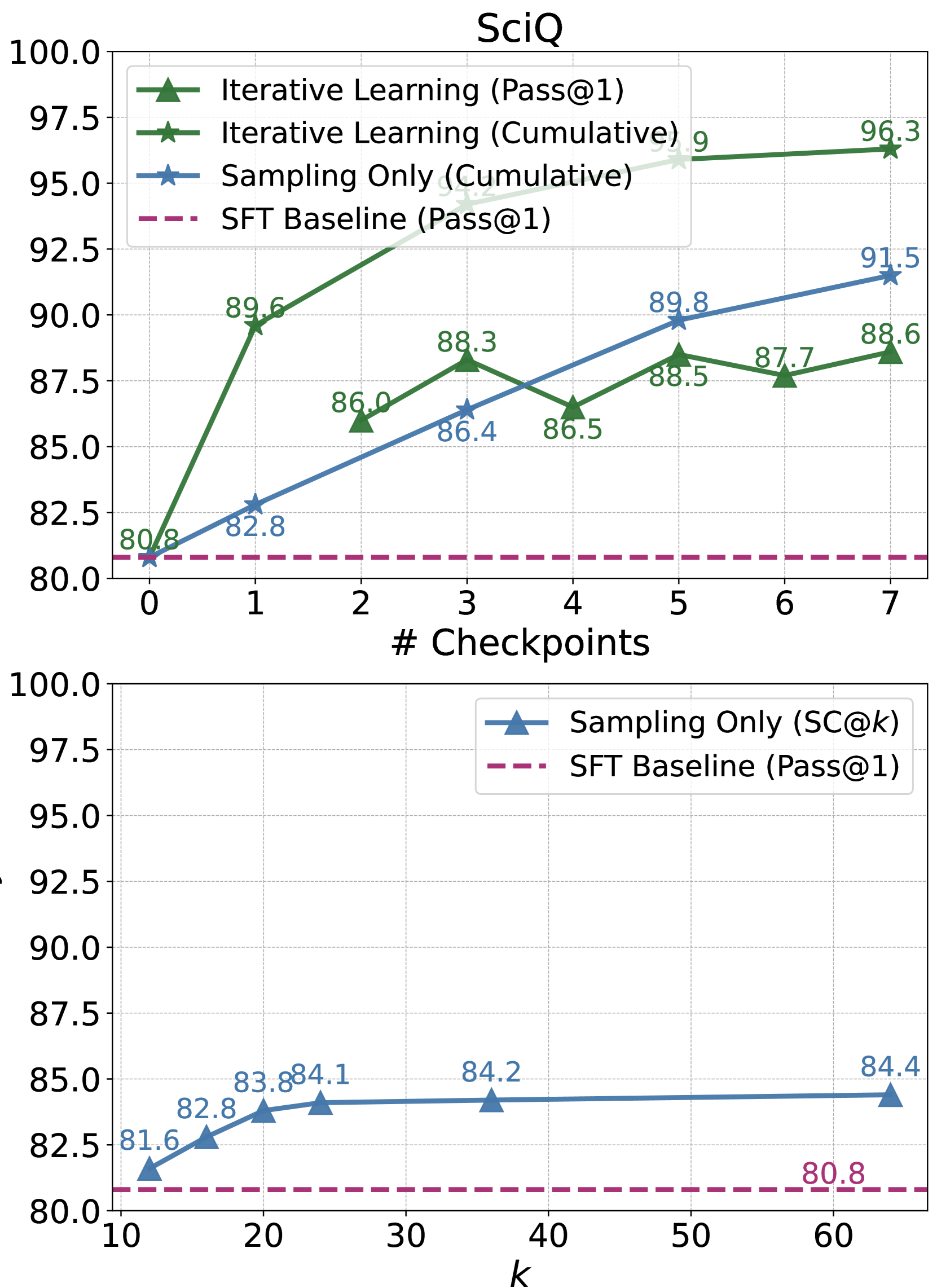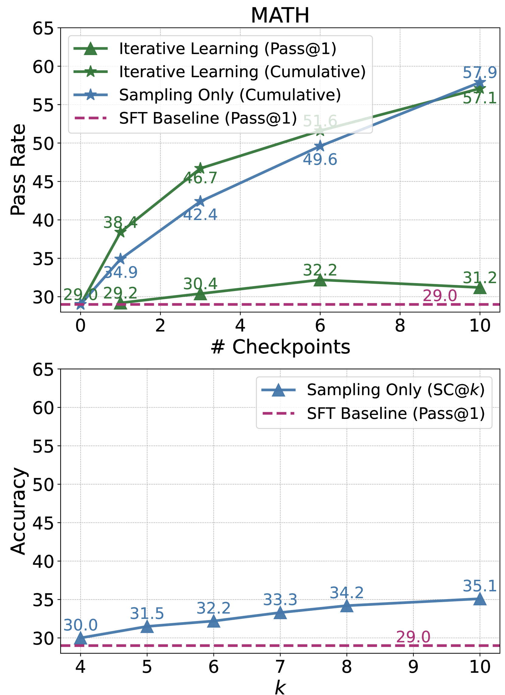</details> Figure 3: Training- vs. Test- Time Compute Scaling on ARC-C, SciQ, and MATH evaluation sets. The cumulative pass rate of our iterative learning method can be seen as the pass rate of an ensemble of different model checkpoints. We use greedy decoding to obtain the inference time performance of our method of iterative learning. Table 3: Ablation of “EXAMPLE ANSWER” in self-evaluation on GSM8K, MATH, and ARC-C. We report AUC and accuracy ( $\%$ ) to compare the discriminative abilities of self-evaluation scores. | w/ example answer-w/o example answer | $74.7$ $62.0$ | $72.5$ $69.5$ | $76.6$ $48.1$ | $48.8$ $42.3$ | $65.2$ $55.8$ | $57.5$ $48.4$ | | --- | --- | --- | --- | --- | --- | --- | Commonsense Reasoning. In Table 2, we report the performance on commonsense reasoning tasks, where our method shows consistent improvements. Notably, we achieve absolute accuracy increases of $2.5\%$ , $3.0\%$ , and $2.1\%$ on ARC-Challenge (ARC-C), AI2Sci-Middle (AI2Sci-M), and SciQ, respectively, surpassing the results of direct tuning. However, in tasks like OBQA and CSQA, our method, focusing on intermediate reasoning refinement, is less efficient compared to direct tuning. Despite significant improvements over the Supervised Fine-Tuning (SFT) baseline (for instance, from $59.8\%$ to $79.2\%$ on OBQA, and from $54.1\%$ to $74.8\%$ on CSQA), the gains are modest relative to direct tuning. This discrepancy could be attributed to the base model’s lack of specific knowledge, where eliciting intermediate reasoning chains may introduce increased uncertainty in model generations, leading to incorrect predictions. We delve deeper into this issue of hallucination and its implications in our qualitative analysis, as detailed in Section 4.2. 4.2 Further Analysis Training- vs. Test- Time Compute Scaling. Our method integrates MCTS with preference learning, aiming to enhance both preference quality and policy reasoning via step-level alignment. We analyze the impact of training-time compute scaling versus increased inference-time sampling. We measure success by the pass rate, indicating the percentage of correctly elicited answers. Figure 3 displays the cumulative pass rate at each checkpoint, aggregating the pass rates up to that point. For test-time scaling, we increase the number of sampled reasoning chains. Additionally, we compare the inference performance of our checkpoints with a sampling-only method, self-consistency, to assess their potential performance ceilings. The pass rate curves on ARC-C, SciQ, and MATH datasets reveal that our MCTS-enhanced approach yields a higher training compute scaling exponent. This effect is particularly pronounced on the unseen SciQ dataset, highlighting our method’s efficiency and effectiveness in enhancing specific reasoning abilities with broad applicability. Inference-time performance analysis shows higher performance upper bounds of our method on ARC-C and SciQ. For instance, while self-consistency on SciQ plateaus at around $84\%$ , our framework pushes performance to $88.6\%$ . However, on MATH, the sampling-only approach outperforms training compute scaling: more sampling consistently enhances performance beyond $35\%$ , whereas post-training performance hovers around $32.2\%$ . This observation suggests that in-domain SFT already aligns the model well with task-specific requirements. Functions of Self-Evaluation Mechanism. As illustrated in Section 2.1, the self-evaluation score inherently revises the $Q$ value estimation for subsequent preference data collection. In practice, we find that the ground-truth information, i.e., the “EXAMPLE ANSWER” in Table 6, is crucial to ensure the reliability of self-evaluation. We now compare the score distribution and discriminative abilities when including v.s. excluding this ground-truth information in Table 3. With this information , the accuracy of self-evaluation significantly improves across GSM8K, MATH, and ARC-C datasets. Ablation Study. We ablate the impact of step-level supervision signals and the online learning aspect of our MCTS-based approach. Tables 1 and 2 shows performance comparisons across commonsense and arithmetic reasoning tasks under different settings. Our method, focusing on step-level online preference learning, consistently outperforms both instance-level and offline approaches in commonsense reasoning. For example, we achieve $76.4\%$ on ARC-C and $88.5\%$ on SciQ, surpassing $70.8\%$ and $87.4\%$ of the offline variant, and $75.3\%$ and $87.6\%$ of the instance-level approach. <details> <summary>x7.png Details</summary>  ### Visual Description ## Bar Chart: Model Accuracy Comparison Across Tasks and Evaluation Levels ### Overview The chart compares accuracy percentages of three models (Initial Model, Trained Model, G.T. Supervision) across two tasks (ARC-C, MATH) and two evaluation levels (step-level, instance-level). A fifth category combines MATH step-level with ground truth supervision (G.T.). The y-axis represents accuracy (0-100%), while the x-axis categorizes tasks and evaluation types. ### Components/Axes - **X-axis**: - Categories: 1. ARC-C (step-level) 2. ARC-C (instance-level) 3. MATH (step-level) 4. MATH (instance-level) 5. MATH (step-level w/ G.T.) - **Y-axis**: Accuracy (0-100%, increments of 20) - **Legend**: - Orange: Initial Model - Blue: Trained Model - Green: G.T. Supervision - **Bar Values**: Numerical accuracy percentages displayed atop each bar. ### Detailed Analysis 1. **ARC-C (step-level)**: - Initial Model: 60.6% - Trained Model: 76.4% - G.T. Supervision: 94.4% 2. **ARC-C (instance-level)**: - Initial Model: 60.6% - Trained Model: 75.3% - G.T. Supervision: 89.2% 3. **MATH (step-level)**: - Initial Model: 29.0% - Trained Model: 32.2% - G.T. Supervision: 81.2% 4. **MATH (instance-level)**: - Initial Model: 29.0% - Trained Model: 32.9% - G.T. Supervision: 87.9% 5. **MATH (step-level w/ G.T.)**: - Initial Model: 29.0% - Trained Model: 35.4% - G.T. Supervision: 97.9% ### Key Observations - **G.T. Supervision Dominance**: Green bars (G.T. Supervision) consistently show the highest accuracy across all categories, reaching 97.9% in MATH step-level with G.T. - **Trained Model vs. Initial Model**: Blue bars (Trained Model) outperform orange bars (Initial Model) in all cases, with the largest gap in MATH step-level w/ G.T. (35.4% vs. 29.0%). - **Task-Specific Trends**: - ARC-C tasks show higher baseline accuracy than MATH tasks. - Instance-level evaluations for ARC-C slightly underperform step-level (e.g., 89.2% vs. 94.4% for G.T. Supervision). - MATH instance-level accuracy surpasses step-level for G.T. Supervision (87.9% vs. 81.2%). ### Interpretation The data demonstrates that **ground truth supervision (G.T.) is critical for high accuracy**, particularly in complex tasks like MATH. The Trained Model improves upon the Initial Model but remains significantly outperformed by G.T. supervision. Notably, MATH step-level with G.T. achieves near-perfect accuracy (97.9%), suggesting that combining step-level evaluation with ground truth yields optimal results. The disparity between Initial and Trained Models highlights the value of model training, while the consistent G.T. superiority underscores its role as a benchmark. The instance-level vs. step-level performance differences may reflect task complexity or evaluation methodology nuances. 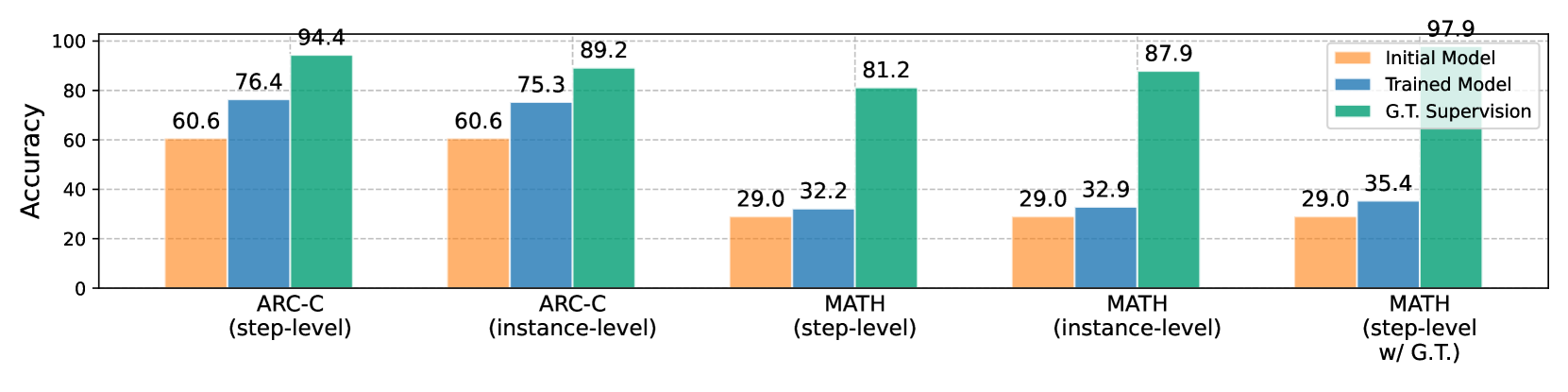</details> Figure 4: Abltation study on step- vs. instance-level supervision, online vs. offline learning, and w/ vs. w/o G.T. supervision. We also compare the accuracy of the training signals collected via MCTS or instance-level sampling. Table 4: Qualitative Analysis of model outputs on OBQA, AI2Sci, and MATH. We highlight correct and incorrect keywords. The predicted answers on MATH are boxed, where our method solves the complex problem while SFT baseline failed to elicit a complete reasoning chain. $$ f(x)=x^{7}+ax^{3}+cx f(5)=3, f(-5) f(5)=5^{7}+5a+5c=3. f(-5), (-5)^{7}+(-5a) +(-5c). (-5)^{7}=-5^{7}=-3, f(-5)=-3-5a-5c. f(-5)=-3-5(-3)-5c=-3+15-5c=\boxed{{\color[rgb]{0.609375,0.37890625,0.71875}12-% 5c}}. f(5)=5^{7}+5a+5c=3. f(x) f(-5)=(-5)^{7}-5a-5c=\boxed{{\color[rgb]{0,0.88,0}-3}}. f(c)=\frac{3}{2c-3} \frac{kn^{2}}{lm} f^{-1}(c)\times c\times f(c) \frac{kc+l}{mc+n} k,l,m,\text{ and }n f^{-1}(c) f(c)=x c \frac{3}{2c-3}=x 2c-3=\frac{3}{x} 2c=\frac{3}{x}+3 c=\frac{\frac{3}{x}+3}{2} f^{-1}(c)=\frac{\frac{3}{c}+3}{2c} f^{-1}(c) f^{-1}(c)\times c\times f(c) \frac{\frac{3}{c}+3}{2c}\times c\times\frac{3}{2c-3} \frac{3+3c}{2c}\times\frac{3}{2c-3} \frac{9+9c}{4c^{2}-6c} \frac{9+9c}{4c(c-1)} \frac{kc+l}{mc+n} k,l,m, n \frac{9+9c}{4c(c-1)}=\frac{kc+l}{mc+n} 9+9c=4c(c-1)(kc+l) 9+9c=4c^{2}k-4ck-4cl+l 4c^{2}k-4 f(f^{-1}(c))=c c f^{-1} f(f^{-1}(c))=f(c) c f^{-1} f(f^{-1}(c))=f(c) f(c)=c c f^{-1} f(c)=\frac{3}{2c-3} f(c)=c c f^{-1} 2c-3=c c f^{-1} c=3 c f^{-1} f^{-1}(c)=3 c f^{-1} f^{-1}(c)=3 f^{-1}(c)\times c\times f(c) 3\times 3\times\frac{3}{2(3)-3} 9\times\frac{3}{3}=9 \frac{kn^{2}}{lm}=\boxed{{\color[rgb]{0,0.88,0}9}} \tag{5} $$ In arithmetic reasoning, performance differences among settings are less pronounced for challenging task such as MATH without the incorporation of ground-truth solutions (e.g., $32.2\%$ for our method (w/o G.T.) vs. $31.9\%$ and $32.9\%$ for offline and instance-level on MATH). The comparable performance of offline learning aligns with our theoretical analysis that offline approaches can be effective when the initial policy is already well-tuned with high-quality, in-domain data. We further interpret how G.T. guidance integration to enhance the effectiveness of our framework in Figure 4. With G.T. supervision, the accuracy of training signals improve significantly from $81.2\%$ to $97.9\%$ , leading to substantial performance gain on model performance. This also explains the similar performance (w/o G.T.) between corresponding using step- and instance-level supervision, where our step-level approach shows effectiveness in narrowing the gap between accuracies of corresponding supervisions. Training Dynamics in Iterative Learning. As shown in Figure 2, online learning exhibits cyclic performance fluctuations, with validation performance peaking before dipping. We conduct theoretical analysis on this in Appendix B and shows that continuous policy updates with the latest models can lead to periodic knowledge loss due to insufficient optimization in iterative updates. We further probe these phenomena qualitatively next. Qualitative Analysis. Our qualitative analysis in Table 4 examines the impact of step-level supervision on intermediate reasoning correctness across different tasks. In OBQA, the implementation of MCTS, as discussed in Section 4.1, often leads to longer reasoning chains. This can introduce errors in commonsense reasoning tasks, as seen in our OBQA example, where an extended chain results in an incorrect final prediction. Conversely, in the MATH dataset, our approach successfully guides the model to rectify mistakes and formulates accurate, extended reasoning chains, demonstrating its effectiveness in complex math word problems. This analysis underscores the need to balance reasoning chain length and logical coherence, particularly in tasks with higher uncertainty, such as commonsense reasoning. 5 Related Work Various studies focus on self-improvement to exploit the model’s capability. One line of work focuses on collecting high-quality positive data from model generations guided by static reward heuristic (Zelikman et al., 2022; Gülçehre et al., 2023; Polu et al., 2023). Recently, Yuan et al. (2024) utilize the continuously updated LLM self-rewarding to collect both positive and negative data for preference learning. Fu et al. (2023) adopt exploration strategy via rejection sampling to do online data collection for iterative preference learning. Different from prior works at instance-level alignment, we leverage MCTS as a policy improvement operator to iteratively facilitate step-level preference learning. We discuss additional related work in Appendix A. 6 Conclusion In this paper, we propose MCTS-enhanced iterative preference learning, utilizing MCTS as a policy improvement operator to enhance LLM alignment via step-level preference learning. MCTS balances quality exploitation and diversity exploration to produce high-quality training data, efficiently pushing the ceiling performance of the LLM on various reasoning tasks. Theoretical analysis shows that online sampling in our iterative learning framework is key to improving the LLM policy toward optimal alignment. We hope our proposed approach can inspire future research on LLM alignment from both data-centric and algorithm-improving aspects: to explore searching strategies and utilization of history data and policies to augment and diversify training examples; to strategically employ a tradeoff between offline and online learning to address the problem of cyclic performance change of the online learning framework as discussed in our theoretical analysis. Acknowledgments and Disclosure of Funding The computational work for this article was partially performed on resources of the National Supercomputing Centre (NSCC), Singapore https://www.nscc.sg/. References - Anthony et al. (2017) Thomas Anthony, Zheng Tian, and David Barber. 2017. Thinking fast and slow with deep learning and tree search. In Advances in Neural Information Processing Systems 30: Annual Conference on Neural Information Processing Systems 2017, December 4-9, 2017, Long Beach, CA, USA, pages 5360–5370. - Azar et al. (2023) Mohammad Gheshlaghi Azar, Mark Rowland, Bilal Piot, Daniel Guo, Daniele Calandriello, Michal Valko, and Rémi Munos. 2023. A general theoretical paradigm to understand learning from human preferences. CoRR, abs/2310.12036. - Bai et al. (2022a) Yuntao Bai, Andy Jones, Kamal Ndousse, Amanda Askell, Anna Chen, Nova DasSarma, Dawn Drain, Stanislav Fort, Deep Ganguli, Tom Henighan, Nicholas Joseph, Saurav Kadavath, Jackson Kernion, Tom Conerly, Sheer El Showk, Nelson Elhage, Zac Hatfield-Dodds, Danny Hernandez, Tristan Hume, Scott Johnston, Shauna Kravec, Liane Lovitt, Neel Nanda, Catherine Olsson, Dario Amodei, Tom B. Brown, Jack Clark, Sam McCandlish, Chris Olah, Benjamin Mann, and Jared Kaplan. 2022a. Training a helpful and harmless assistant with reinforcement learning from human feedback. CoRR, abs/2204.05862. - Bai et al. (2022b) Yuntao Bai, Saurav Kadavath, Sandipan Kundu, Amanda Askell, Jackson Kernion, Andy Jones, Anna Chen, Anna Goldie, Azalia Mirhoseini, Cameron McKinnon, et al. 2022b. Constitutional ai: Harmlessness from ai feedback. arXiv preprint arXiv:2212.08073. - Bradley and Terry (1952) Ralph Allan Bradley and Milton E Terry. 1952. Rank analysis of incomplete block designs: I. the method of paired comparisons. Biometrika, 39(3/4):324–345. - Brown et al. (2020) Tom Brown, Benjamin Mann, Nick Ryder, Melanie Subbiah, Jared D Kaplan, Prafulla Dhariwal, Arvind Neelakantan, Pranav Shyam, Girish Sastry, Amanda Askell, et al. 2020. Language models are few-shot learners. Advances in neural information processing systems, 33:1877–1901. - Christiano et al. (2017) Paul F. Christiano, Jan Leike, Tom B. Brown, Miljan Martic, Shane Legg, and Dario Amodei. 2017. Deep reinforcement learning from human preferences. In Advances in Neural Information Processing Systems 30: Annual Conference on Neural Information Processing Systems 2017, December 4-9, 2017, Long Beach, CA, USA, pages 4299–4307. - Clark et al. (2018) Peter Clark, Isaac Cowhey, Oren Etzioni, Tushar Khot, Ashish Sabharwal, Carissa Schoenick, and Oyvind Tafjord. 2018. Think you have solved question answering? try arc, the AI2 reasoning challenge. CoRR, abs/1803.05457. - Cobbe et al. (2021) Karl Cobbe, Vineet Kosaraju, Mohammad Bavarian, Mark Chen, Heewoo Jun, Lukasz Kaiser, Matthias Plappert, Jerry Tworek, Jacob Hilton, Reiichiro Nakano, Christopher Hesse, and John Schulman. 2021. Training verifiers to solve math word problems. CoRR, abs/2110.14168. - Coulom (2006) Rémi Coulom. 2006. Efficient selectivity and backup operators in monte-carlo tree search. In International conference on computers and games, pages 72–83. Springer. - Fu et al. (2023) Chaoyou Fu, Peixian Chen, Yunhang Shen, Yulei Qin, Mengdan Zhang, Xu Lin, Zhenyu Qiu, Wei Lin, Jinrui Yang, Xiawu Zheng, Ke Li, Xing Sun, and Rongrong Ji. 2023. MME: A comprehensive evaluation benchmark for multimodal large language models. CoRR, abs/2306.13394. - Grill et al. (2020) Jean-Bastien Grill, Florent Altché, Yunhao Tang, Thomas Hubert, Michal Valko, Ioannis Antonoglou, and Rémi Munos. 2020. Monte-carlo tree search as regularized policy optimization. In International Conference on Machine Learning, pages 3769–3778. PMLR. - Gülçehre et al. (2023) Çaglar Gülçehre, Tom Le Paine, Srivatsan Srinivasan, Ksenia Konyushkova, Lotte Weerts, Abhishek Sharma, Aditya Siddhant, Alex Ahern, Miaosen Wang, Chenjie Gu, Wolfgang Macherey, Arnaud Doucet, Orhan Firat, and Nando de Freitas. 2023. Reinforced self-training (rest) for language modeling. CoRR, abs/2308.08998. - Hao et al. (2023) Shibo Hao, Yi Gu, Haodi Ma, Joshua Jiahua Hong, Zhen Wang, Daisy Zhe Wang, and Zhiting Hu. 2023. Reasoning with language model is planning with world model. In Proceedings of the 2023 Conference on Empirical Methods in Natural Language Processing, EMNLP 2023, Singapore, December 6-10, 2023, pages 8154–8173. Association for Computational Linguistics. - He et al. (2020) Junxian He, Jiatao Gu, Jiajun Shen, and Marc’Aurelio Ranzato. 2020. Revisiting self-training for neural sequence generation. In 8th International Conference on Learning Representations, ICLR 2020, Addis Ababa, Ethiopia, April 26-30, 2020. OpenReview.net. - Hendrycks et al. (2021) Dan Hendrycks, Collin Burns, Saurav Kadavath, Akul Arora, Steven Basart, Eric Tang, Dawn Song, and Jacob Steinhardt. 2021. Measuring mathematical problem solving with the MATH dataset. In Proceedings of the Neural Information Processing Systems Track on Datasets and Benchmarks 1, NeurIPS Datasets and Benchmarks 2021, December 2021, virtual. - Huang et al. (2023) Jiaxin Huang, Shixiang Gu, Le Hou, Yuexin Wu, Xuezhi Wang, Hongkun Yu, and Jiawei Han. 2023. Large language models can self-improve. In Proceedings of the 2023 Conference on Empirical Methods in Natural Language Processing, EMNLP 2023, Singapore, December 6-10, 2023, pages 1051–1068. Association for Computational Linguistics. - III (1965) H. J. Scudder III. 1965. Probability of error of some adaptive pattern-recognition machines. IEEE Trans. Inf. Theory, 11(3):363–371. - Jiang et al. (2023) Albert Q. Jiang, Alexandre Sablayrolles, Arthur Mensch, Chris Bamford, Devendra Singh Chaplot, Diego de Las Casas, Florian Bressand, Gianna Lengyel, Guillaume Lample, Lucile Saulnier, Lélio Renard Lavaud, Marie-Anne Lachaux, Pierre Stock, Teven Le Scao, Thibaut Lavril, Thomas Wang, Timothée Lacroix, and William El Sayed. 2023. Mistral 7b. CoRR, abs/2310.06825. - Kadavath et al. (2022) Saurav Kadavath, Tom Conerly, Amanda Askell, Tom Henighan, Dawn Drain, Ethan Perez, Nicholas Schiefer, Zac Hatfield-Dodds, Nova DasSarma, Eli Tran-Johnson, Scott Johnston, Sheer El Showk, Andy Jones, Nelson Elhage, Tristan Hume, Anna Chen, Yuntao Bai, Sam Bowman, Stanislav Fort, Deep Ganguli, Danny Hernandez, Josh Jacobson, Jackson Kernion, Shauna Kravec, Liane Lovitt, Kamal Ndousse, Catherine Olsson, Sam Ringer, Dario Amodei, Tom Brown, Jack Clark, Nicholas Joseph, Ben Mann, Sam McCandlish, Chris Olah, and Jared Kaplan. 2022. Language models (mostly) know what they know. CoRR, abs/2207.05221. - Kocsis and Szepesvári (2006) Levente Kocsis and Csaba Szepesvári. 2006. Bandit based monte-carlo planning. In European conference on machine learning, pages 282–293. Springer. - Lee et al. (2023) Harrison Lee, Samrat Phatale, Hassan Mansoor, Kellie Lu, Thomas Mesnard, Colton Bishop, Victor Carbune, and Abhinav Rastogi. 2023. RLAIF: scaling reinforcement learning from human feedback with AI feedback. CoRR, abs/2309.00267. - Li et al. (2023) Yifei Li, Zeqi Lin, Shizhuo Zhang, Qiang Fu, Bei Chen, Jian-Guang Lou, and Weizhu Chen. 2023. Making language models better reasoners with step-aware verifier. In Proceedings of the 61st Annual Meeting of the Association for Computational Linguistics (Volume 1: Long Papers), pages 5315–5333. - Lightman et al. (2023) Hunter Lightman, Vineet Kosaraju, Yura Burda, Harrison Edwards, Bowen Baker, Teddy Lee, Jan Leike, John Schulman, Ilya Sutskever, and Karl Cobbe. 2023. Let’s verify step by step. CoRR, abs/2305.20050. - Liu et al. (2023a) Jiacheng Liu, Andrew Cohen, Ramakanth Pasunuru, Yejin Choi, Hannaneh Hajishirzi, and Asli Celikyilmaz. 2023a. Making PPO even better: Value-guided monte-carlo tree search decoding. CoRR, abs/2309.15028. - Liu et al. (2023b) Jiacheng Liu, Ramakanth Pasunuru, Hannaneh Hajishirzi, Yejin Choi, and Asli Celikyilmaz. 2023b. Crystal: Introspective reasoners reinforced with self-feedback. In Proceedings of the 2023 Conference on Empirical Methods in Natural Language Processing, pages 11557–11572, Singapore. Association for Computational Linguistics. - Liu et al. (2023c) Tianqi Liu, Yao Zhao, Rishabh Joshi, Misha Khalman, Mohammad Saleh, Peter J. Liu, and Jialu Liu. 2023c. Statistical rejection sampling improves preference optimization. CoRR, abs/2309.06657. - Mihaylov et al. (2018) Todor Mihaylov, Peter Clark, Tushar Khot, and Ashish Sabharwal. 2018. Can a suit of armor conduct electricity? A new dataset for open book question answering. In Proceedings of the 2018 Conference on Empirical Methods in Natural Language Processing, Brussels, Belgium, October 31 - November 4, 2018, pages 2381–2391. Association for Computational Linguistics. - Mitchell (2023) Eric Mitchell. 2023. A note on dpo with noisy preferences & relationship to ipo. - Ouyang et al. (2022) Long Ouyang, Jeffrey Wu, Xu Jiang, Diogo Almeida, Carroll L. Wainwright, Pamela Mishkin, Chong Zhang, Sandhini Agarwal, Katarina Slama, Alex Ray, John Schulman, Jacob Hilton, Fraser Kelton, Luke Miller, Maddie Simens, Amanda Askell, Peter Welinder, Paul F. Christiano, Jan Leike, and Ryan Lowe. 2022. Training language models to follow instructions with human feedback. In NeurIPS. - Park et al. (2020) Daniel S Park, Yu Zhang, Ye Jia, Wei Han, Chung-Cheng Chiu, Bo Li, Yonghui Wu, and Quoc V Le. 2020. Improved noisy student training for automatic speech recognition. arXiv preprint arXiv:2005.09629. - Polu et al. (2023) Stanislas Polu, Jesse Michael Han, Kunhao Zheng, Mantas Baksys, Igor Babuschkin, and Ilya Sutskever. 2023. Formal mathematics statement curriculum learning. In The Eleventh International Conference on Learning Representations, ICLR 2023, Kigali, Rwanda, May 1-5, 2023. OpenReview.net. - Rafailov et al. (2023) Rafael Rafailov, Archit Sharma, Eric Mitchell, Stefano Ermon, Christopher D. Manning, and Chelsea Finn. 2023. Direct preference optimization: Your language model is secretly a reward model. CoRR, abs/2305.18290. - Raffel et al. (2020) Colin Raffel, Noam Shazeer, Adam Roberts, Katherine Lee, Sharan Narang, Michael Matena, Yanqi Zhou, Wei Li, and Peter J Liu. 2020. Exploring the limits of transfer learning with a unified text-to-text transformer. The Journal of Machine Learning Research, 21(1):5485–5551. - Ren et al. (2023) Jie Ren, Yao Zhao, Tu Vu, Peter J Liu, and Balaji Lakshminarayanan. 2023. Self-evaluation improves selective generation in large language models. arXiv preprint arXiv:2312.09300. - Rosin (2011) Christopher D Rosin. 2011. Multi-armed bandits with episode context. Annals of Mathematics and Artificial Intelligence, 61(3):203–230. - Schulman et al. (2017) John Schulman, Filip Wolski, Prafulla Dhariwal, Alec Radford, and Oleg Klimov. 2017. Proximal policy optimization algorithms. CoRR, abs/1707.06347. - Silver et al. (2017) David Silver, Thomas Hubert, Julian Schrittwieser, Ioannis Antonoglou, Matthew Lai, Arthur Guez, Marc Lanctot, Laurent Sifre, Dharshan Kumaran, Thore Graepel, Timothy P. Lillicrap, Karen Simonyan, and Demis Hassabis. 2017. Mastering chess and shogi by self-play with a general reinforcement learning algorithm. CoRR, abs/1712.01815. - Stiennon et al. (2020) Nisan Stiennon, Long Ouyang, Jeff Wu, Daniel M. Ziegler, Ryan Lowe, Chelsea Voss, Alec Radford, Dario Amodei, and Paul F. Christiano. 2020. Learning to summarize from human feedback. CoRR, abs/2009.01325. - Talmor et al. (2019) Alon Talmor, Jonathan Herzig, Nicholas Lourie, and Jonathan Berant. 2019. CommonsenseQA: A question answering challenge targeting commonsense knowledge. In Proceedings of the 2019 Conference of the North American Chapter of the Association for Computational Linguistics: Human Language Technologies, Volume 1 (Long and Short Papers), pages 4149–4158, Minneapolis, Minnesota. Association for Computational Linguistics. - Touvron et al. (2023) Hugo Touvron, Louis Martin, Kevin Stone, Peter Albert, Amjad Almahairi, Yasmine Babaei, Nikolay Bashlykov, Soumya Batra, Prajjwal Bhargava, Shruti Bhosale, Dan Bikel, Lukas Blecher, Cristian Canton-Ferrer, Moya Chen, Guillem Cucurull, David Esiobu, Jude Fernandes, Jeremy Fu, Wenyin Fu, Brian Fuller, Cynthia Gao, Vedanuj Goswami, Naman Goyal, Anthony Hartshorn, Saghar Hosseini, Rui Hou, Hakan Inan, Marcin Kardas, Viktor Kerkez, Madian Khabsa, Isabel Kloumann, Artem Korenev, Punit Singh Koura, Marie-Anne Lachaux, Thibaut Lavril, Jenya Lee, Diana Liskovich, Yinghai Lu, Yuning Mao, Xavier Martinet, Todor Mihaylov, Pushkar Mishra, Igor Molybog, Yixin Nie, Andrew Poulton, Jeremy Reizenstein, Rashi Rungta, Kalyan Saladi, Alan Schelten, Ruan Silva, Eric Michael Smith, Ranjan Subramanian, Xiaoqing Ellen Tan, Binh Tang, Ross Taylor, Adina Williams, Jian Xiang Kuan, Puxin Xu, Zheng Yan, Iliyan Zarov, Yuchen Zhang, Angela Fan, Melanie Kambadur, Sharan Narang, Aurélien Rodriguez, Robert Stojnic, Sergey Edunov, and Thomas Scialom. 2023. Llama 2: Open foundation and fine-tuned chat models. CoRR, abs/2307.09288. - Uesato et al. (2022) Jonathan Uesato, Nate Kushman, Ramana Kumar, H. Francis Song, Noah Y. Siegel, Lisa Wang, Antonia Creswell, Geoffrey Irving, and Irina Higgins. 2022. Solving math word problems with process- and outcome-based feedback. CoRR, abs/2211.14275. - Wang and Komatsuzaki (2021) Ben Wang and Aran Komatsuzaki. 2021. GPT-J-6B: A 6 Billion Parameter Autoregressive Language Model. https://github.com/kingoflolz/mesh-transformer-jax. - Wang et al. (2023a) Peiyi Wang, Lei Li, Zhihong Shao, RX Xu, Damai Dai, Yifei Li, Deli Chen, Y Wu, and Zhifang Sui. 2023a. Math-shepherd: A label-free step-by-step verifier for llms in mathematical reasoning. arXiv preprint arXiv:2312.08935. - Wang et al. (2023b) Xuezhi Wang, Jason Wei, Dale Schuurmans, Quoc V. Le, Ed H. Chi, Sharan Narang, Aakanksha Chowdhery, and Denny Zhou. 2023b. Self-consistency improves chain of thought reasoning in language models. In The Eleventh International Conference on Learning Representations, ICLR 2023, Kigali, Rwanda, May 1-5, 2023. OpenReview.net. - Wei et al. (2022) Jason Wei, Xuezhi Wang, Dale Schuurmans, Maarten Bosma, Brian Ichter, Fei Xia, Ed H. Chi, Quoc V. Le, and Denny Zhou. 2022. Chain-of-thought prompting elicits reasoning in large language models. In Advances in Neural Information Processing Systems 35: Annual Conference on Neural Information Processing Systems 2022, NeurIPS 2022, New Orleans, LA, USA, November 28 - December 9, 2022. - Welbl et al. (2017) Johannes Welbl, Nelson F. Liu, and Matt Gardner. 2017. Crowdsourcing multiple choice science questions. In Proceedings of the 3rd Workshop on Noisy User-generated Text, NUT@EMNLP 2017, Copenhagen, Denmark, September 7, 2017, pages 94–106. Association for Computational Linguistics. - Wu et al. (2023) Zeqiu Wu, Yushi Hu, Weijia Shi, Nouha Dziri, Alane Suhr, Prithviraj Ammanabrolu, Noah A. Smith, Mari Ostendorf, and Hannaneh Hajishirzi. 2023. Fine-grained human feedback gives better rewards for language model training. CoRR, abs/2306.01693. - Xie et al. (2020) Qizhe Xie, Minh-Thang Luong, Eduard H. Hovy, and Quoc V. Le. 2020. Self-training with noisy student improves imagenet classification. In 2020 IEEE/CVF Conference on Computer Vision and Pattern Recognition, CVPR 2020, Seattle, WA, USA, June 13-19, 2020, pages 10684–10695. Computer Vision Foundation / IEEE. - Xie et al. (2023) Yuxi Xie, Kenji Kawaguchi, Yiran Zhao, Xu Zhao, Min-Yen Kan, Junxian He, and Qizhe Xie. 2023. Decomposition enhances reasoning via self-evaluation guided decoding. CoRR, abs/2305.00633. - Yao et al. (2023) Shunyu Yao, Dian Yu, Jeffrey Zhao, Izhak Shafran, Thomas L. Griffiths, Yuan Cao, and Karthik Narasimhan. 2023. Tree of thoughts: Deliberate problem solving with large language models. CoRR, abs/2305.10601. - Yarowsky (1995) David Yarowsky. 1995. Unsupervised word sense disambiguation rivaling supervised methods. In 33rd Annual Meeting of the Association for Computational Linguistics, 26-30 June 1995, MIT, Cambridge, Massachusetts, USA, Proceedings, pages 189–196. Morgan Kaufmann Publishers / ACL. - Yu et al. (2023a) Fei Yu, Anningzhe Gao, and Benyou Wang. 2023a. Outcome-supervised verifiers for planning in mathematical reasoning. CoRR, abs/2311.09724. - Yu et al. (2023b) Longhui Yu, Weisen Jiang, Han Shi, Jincheng Yu, Zhengying Liu, Yu Zhang, James T Kwok, Zhenguo Li, Adrian Weller, and Weiyang Liu. 2023b. Metamath: Bootstrap your own mathematical questions for large language models. arXiv preprint arXiv:2309.12284. - Yuan et al. (2024) Weizhe Yuan, Richard Yuanzhe Pang, Kyunghyun Cho, Sainbayar Sukhbaatar, Jing Xu, and Jason Weston. 2024. Self-rewarding language models. arXiv preprint arXiv:2401.10020. - Zelikman et al. (2022) Eric Zelikman, Yuhuai Wu, Jesse Mu, and Noah D. Goodman. 2022. Star: Bootstrapping reasoning with reasoning. In NeurIPS. - Zhang et al. (2023) Tianjun Zhang, Fangchen Liu, Justin Wong, Pieter Abbeel, and Joseph E. Gonzalez. 2023. The wisdom of hindsight makes language models better instruction followers. In International Conference on Machine Learning, ICML 2023, 23-29 July 2023, Honolulu, Hawaii, USA, volume 202 of Proceedings of Machine Learning Research, pages 41414–41428. PMLR. - Zheng et al. (2023) Lianmin Zheng, Wei-Lin Chiang, Ying Sheng, Siyuan Zhuang, Zhanghao Wu, Yonghao Zhuang, Zi Lin, Zhuohan Li, Dacheng Li, Eric P. Xing, Hao Zhang, Joseph E. Gonzalez, and Ion Stoica. 2023. Judging llm-as-a-judge with mt-bench and chatbot arena. CoRR, abs/2306.05685. - Zhu et al. (2023) Xinyu Zhu, Junjie Wang, Lin Zhang, Yuxiang Zhang, Yongfeng Huang, Ruyi Gan, Jiaxing Zhang, and Yujiu Yang. 2023. Solving math word problems via cooperative reasoning induced language models. In Proceedings of the 61st Annual Meeting of the Association for Computational Linguistics (Volume 1: Long Papers), ACL 2023, Toronto, Canada, July 9-14, 2023, pages 4471–4485. Association for Computational Linguistics. - Zoph et al. (2020) Barret Zoph, Golnaz Ghiasi, Tsung-Yi Lin, Yin Cui, Hanxiao Liu, Ekin Dogus Cubuk, and Quoc Le. 2020. Rethinking pre-training and self-training. Advances in neural information processing systems, 33:3833–3845. Appendix A Related Work Iterated Learning. Typical iterated learning operates in a multi-agent scenario, consisting of a loop where an apprentice self-plays, learns from expert feedback, and replaces the current expert for the new iteration (Anthony et al., 2017). Polu et al. (2023) apply expert iteration on formal mathematical reasoning to conduct proof search interleaved with learning. Zelikman et al. (2022) avoid the need for training a separate value function by directly assessing the final outcomes of reasoning to filter generated examples for iterated learning. Recently, Yuan et al. (2024) leverage the technique of LLM-as-a-Judge (Zheng et al., 2023) and introduce self-rewarding language models to improve LLM alignment with self-feedback. Differently, we combine the feedback of outcome assessment and LLM self-evaluation and further decompose them into fine-grained signals via MCTS for step-level iterative preference learning. Self-Training. Self-training uses unlabeled data to improve model training by assigning pseudo labels from a learned labeler (III, 1965; Yarowsky, 1995; Xie et al., 2020; He et al., 2020; Park et al., 2020; Zoph et al., 2020). Recent research has explored several alternatives to label the examples. Zelikman et al. (2022) and Gülçehre et al. (2023) use static reward heuristic to curate high-quality examples, while Huang et al. (2023) collect high-confidence outputs as training data via chain-of-thought prompting (Wei et al., 2022) and self-consistency (Wang et al., 2023b). Lee et al. (2023) and Yuan et al. (2024) utilize the off-the-shelf LLM to reward its generations for preference learning. To mitigate the noise from the sparse instance-level signals, we further refine the preference labels via stepwise tree search and LLM self-evaluation. Preference Learning. The empirical achievements of LLMs have identified the benefits of RL techniques to better align with human preferences (Touvron et al., 2023; Stiennon et al., 2020; Ouyang et al., 2022; Bai et al., 2022a). The standard preference learning process learns a reward model to provide feedback in online RL (Schulman et al., 2017). Recently, a variety of studies avoid training separate reward or value networks by hindsight instruction relabeling (Zhang et al., 2023), direct preference optimization (Rafailov et al., 2023) and LLM self-evaluation (Ren et al., 2023). We further explore automatic supervision with MCTS to collect step-level preferences by breaking down outcome correctness integrated with self-evaluation. Our approach enables the continual collection of better-quality data via iterative learning, mitigating the limit of preference data when using a frozen reward model or offline learning algorithms. Guided Search for Reasoning. Recent works improve the LLM reasoning ability by eliciting the intermediate reasoning chain (Wei et al., 2022) and breaking it down into multiple steps via searching (Yao et al., 2023; Hao et al., 2023; Yu et al., 2023a). The decomposition of the reasoning process has also been shown effective in reinforcement learning. Lightman et al. (2023) and Li et al. (2023) apply process supervision to train more reliable reward models than outcome supervision in mathematical reasoning (Uesato et al., 2022). Wang et al. (2023a) reinforce LLMs step-by-step with process supervision data automatically collected via model sampling and annotation. We leverage the look-ahead ability of MCTS and integrate it with step-by-step self-evaluation to provide refined process supervision for reasoning. This improves the generalization ability of our framework to update the policy via real-time collected preferences iteratively. Appendix B Theoretical Analysis of Online DPO Preliminaries. A typical alignment technique begins with a policy $\pi_{\mathrm{sft}}(y\mid x)$ supervisedly fine-tuned on high-quality data from the target domain, where $x$ and $y$ are the prompt and the response, respectively. The SFT policy is used to sample pairs of responses $(y_{1},y_{2})\sim\pi_{\mathrm{sft}}(y\mid x)$ with prompts $x$ , which will be further labeled as pairwise preference data $y_{w}\succ y_{l}\mid x$ , where $y_{w}$ and $y_{l}$ represent the preferred and dispreferred responses respectively. The standard RLHF paradigm trains a reward model (Ouyang et al., 2022) on the preference data and employs PPO (Schulman et al., 2017) to optimize the policy $\pi_{\theta}$ with the feedback provided by the reward model, where $\pi_{\theta}$ is also initialized to $\pi_{\mathrm{sft}}$ in practice. DPO avoids fitting a reward model by optimizing the policy $\pi_{\theta}$ using preferences directly. Given a reward function $r(x,y)$ and prompt distribution $\mathcal{P}$ , RLHF and DPO optimize the KL-constrained reward maximization objective as follows: $$ \max_{\pi}\mathbb{E}_{x\sim\mathcal{P},y\sim\pi}[r(x,y)]-\beta\mathbb{D}_{% \mathrm{KL}}[\pi(y\mid x)\parallel\pi_{\mathrm{sft}}(y\mid x)] \tag{9} $$ where $\beta$ scales the strength of the KL constraint. Let the ground-truth reward function be $r^{*}$ , then Rafailov et al. (2023) estimate the optimal policy $\pi^{*}$ by fitting the Bradley-Terry model (Bradley and Terry, 1952) on preference data: $$ \displaystyle p^{*}(y_{1}\succ y_{1}\mid x)=\sigma(r^{*}(x,y_{1})-r^{*}(x,y_{2% })) \displaystyle= \displaystyle\frac{1}{1+\exp\left(\beta\log\frac{\pi^{*}(y_{2}\mid x)}{\pi_{% \mathrm{sft}}(y_{2}\mid x)}-\beta\log\frac{\pi^{*}(y_{1}\mid x)}{\pi_{\mathrm{% sft}}(y_{1}\mid x)}\right)} \tag{10} $$ As the maximum likelihood estimator (MLE) of the optimal policy requires preferences sampled from the target policy (Liu et al., 2023c), DPO uses a fixed, potentially optimal but unknown policy to collect preference data of good quality. This discrepancy can be a problem when the sampling policy differs dramatically from the current policy. Moreover, the absence of a reward model in DPO presents challenges in learning from additional policy-generated data that lacks explicit preference indicators. We further discuss the offline and online settings of DPO in Section 3. Additional details on labeling outcomes. After a pair of outcomes $(y^{(i)},{y^{\prime}}^{(i)})$ are sampled from some sampling policy $\pi^{(i)}$ , these are labeled to be $y_{w}^{(i)}$ and $y_{l}^{(i)}$ according to some preference density $p$ . That is, $\Pr[(y_{w}^{(i)},y_{l}^{(i)})=(y^{(i)},{y^{\prime}}^{(i)})]=p(y^{(i)}\succ y^{% \prime(i)}\mid x)$ and $\Pr[(y_{w}^{(i)},y_{l}^{(i)})=({y^{\prime}}^{(i)},y^{(i)})]=1-p(y^{(i)}\succ{y% ^{\prime}}^{(i)}\mid x)$ . For simplicity, a preference density is set to be $p(y^{*}\succ\bar{y}\mid x)=1$ for every optima-suboptimal pairs $(y^{*},\bar{y})$ for all $\bar{y}∈ Y$ . We do not specify the preference density for other pairs, i.e., $p(\bar{y}\succ\bar{y}^{\prime}\mid x)$ is arbitrary for $(\bar{y},\bar{y}^{\prime})∈ Y× Y$ . Abstract formulation for both offline and online settings. Our abstract formulation covers both the offline and online settings. The offline setting in previous papers is obtained by setting $\pi^{(i)}$ to be a single distribution fixed over $i∈\{1,2,·s,M\}$ , e.g., an initial policy, an optimal policy, or an empirical data distribution of a given preference data. In the case of the empirical data distribution, the preference density $p$ is set to the function outputting only $0 0$ or $1$ to recover the given preference data. The online setting is obtained by setting $\pi^{(i)}=\pi_{\theta^{(i-1)}}$ where $\pi_{\theta^{(i-1)}}$ is the latest policy at the beginning of the $i$ -th iteration, i.e., for $i≥ 1$ , ${\theta^{(i)}}$ satisfies $\ell_{j}(\theta^{(i)})=0$ for $j∈\{1,2,·s,i-1\}$ and $\theta^{(0)}$ is the initialization. Thus, we can analyze both offline and online settings with this abstract framework. Proof of Theorem 3.1. * Proof* The intuition behind the proof of Theorem 3.1 is that the current policy $\pi_{\theta^{(i)}}$ may not be corrected if a fixed sampling policy $\pi$ never samples a suboptimal output $\bar{y}∈ Y$ whose probability is high for the current policy $\pi_{\theta^{(i)}}$ . Let $\bar{y}$ be the suboptimal output such that $\pi(\bar{y}\mid x)≤\epsilon$ and $\pi_{\theta^{(i)}}(\bar{y}\mid x)≥ c$ for some $i∈\{1,2,·s,M\}$ . Denote preferences sampled by policy $\pi^{(i)}$ as $(y_{w}^{(i)},y_{l}^{(i)})$ . From the definition of the logistic function, we can rewrite | | $\displaystyle\ell_{i}(\theta)$ | $\displaystyle=-\log\sigma\left(\beta\log\frac{\pi_{\theta}(y_{w}^{(i)}\mid x)}% {\pi_{\mathrm{ref}}(y_{w}^{(i)}\mid x)}-\beta\log\frac{\pi_{\theta}(y_{l}^{(i)% }\mid x)}{\pi_{\mathrm{ref}}(y_{l}^{(i)}\mid x)}\right)$ | | | --- | --- | --- | --- | From this equation, we observe that $\ell_{i}(\theta)$ can be minimized to be zero by minimizing $\pi_{\theta}(y_{l}^{(i)}\mid x)$ to be zero without maximizing $\pi_{\theta}(y_{w}^{(i)}\mid x)$ . That is, for any $\beta>0$ , if $\pi_{\theta}(y_{l}^{(i)}\mid x)=0$ , $$ \ell_{i}(\theta)=-\log\frac{\pi_{\theta}(y_{w}^{(i)}\mid x)^{\beta}}{\pi_{% \theta}(y_{w}^{(i)}\mid x)^{\beta}+0}=-\log 1=0. $$ Thus, even if we sample $y^{*}$ with the optimal policy, $\ell_{i}(\theta)$ can be minimized without maximizing $\pi_{\theta}(y^{*}\mid x)$ and minimizing $\pi_{\theta}(\bar{y}|x)$ for $\bar{y}≠ y_{l}^{(i)}$ . Thus, if $\bar{y}≠ y_{l}^{(i)}$ for all $i∈\{1,2,·s,M\}$ , there exists $\theta$ such that $\ell_{i}(\theta)≤ 0$ for all $i=1,...,M$ , and $$ \pi_{\theta}(\bar{y}\mid x)\geq c, $$ because of the condition that $\pi_{\theta}(\bar{y}\mid x)≥ c$ for some $i∈\{1,2,·s,M\}$ : i.e., $\pi_{\theta}(\bar{y}\mid x)$ is never minimized from the $i$ -th iteration while minimizing $\ell_{i}(\theta)$ arbitrarily well, if $\bar{y}$ is never sampled. Therefore, if $\bar{y}$ is never sampled over $m$ iterations, since the probabilities sums up to one, we have $$ \pi_{\theta}(y^{*}\mid x)\leq 1-\pi_{\theta}(\bar{y}|x)\leq 1-c. $$ Moreover, $$ \Pr[\text{\ $\bar{y}$ being never sampled over $m$ iterations }]\geq(1-2% \epsilon)^{m}\geq 1-2\epsilon m, $$ where the last line follows Bernoulli’s inequality. By combining the above two equations, it holds that $$ \Pr[\pi_{\theta}(y^{*}|x)\leq 1-c]\geq 1-2\epsilon M. $$ ∎ Proof of Theorem 3.2. * Proof* From the proof of Theorem 3.1, we have $$ \ell_{i}(\theta)=-\log\frac{\pi_{\theta}(y_{w}^{(i)}\mid x)^{\beta}}{\pi_{% \theta}(y_{w}^{(i)}\mid x)^{\beta}+\pi_{\theta}(y_{l}^{(i)}\mid x)^{\beta}(% \frac{\pi_{\mathrm{ref}}(y_{w}^{(i)}\mid x)}{\pi_{\mathrm{ref}}(y_{l}^{(i)}% \mid x)})^{\beta}}. $$ For $\alpha≥ 0$ and $\beta>0$ , the condition $\ell_{i}(\theta)≤\alpha$ implies that | | $\displaystyle-\log\frac{\pi_{\theta}(y_{w}^{(i)}\mid x)^{\beta}}{\pi_{\theta}(% y_{w}^{(i)}\mid x)^{\beta}+\pi_{\theta}(y_{l}^{(i)}\mid x)^{\beta}(\frac{\pi_{% \mathrm{ref}}(y_{w}^{(i)}\mid x)}{\pi_{\mathrm{ref}}(y_{l}^{(i)}\mid x)})^{% \beta}}≤\alpha$ | | | --- | --- | --- | Since $\pi_{\theta}(y_{w}^{(i)}\mid x)≤ 1$ , this implies that | | $\displaystyle\pi_{\theta}(y_{l}^{(i)}\mid x)$ | $\displaystyle≤\pi_{\theta}(y_{w}^{(i)}\mid x)(\exp(\alpha)-1)^{1/\beta}% \frac{\pi_{\mathrm{ref}}(y_{l}^{(i)}\mid x)}{\pi_{\mathrm{ref}}(y_{w}^{(i)}% \mid x)}$ | | | --- | --- | --- | --- | Thus, while we can prove a similar statement for $\alpha>0$ with this equation, we set $\alpha=0$ for this theorem for a cleaner insight, yielding the following: the condition $\ell_{i}(\theta)≤ 0$ implies that $$ \pi_{\theta}(y_{l}^{(i)}\mid x)=0. $$ Since $y^{(i)}$ and ${y^{\prime}}^{(i)}$ are sampled from $\pi_{\theta^{(i)}}$ without replacement, this means that we have $\pi_{\theta^{(i+k)}}(y_{l}^{(i)}\mid x)=0$ for all $k≥ 1$ from the definition of $\pi_{\theta^{(i)}}$ : i.e., $\pi_{\theta^{(i)}}$ is the policy such that $\ell_{j}(\theta^{(i)})=0$ for all $j=1,...,i-1$ . Since $\pi_{\theta^{(i+k)}}$ is then used to sample $y^{(i)}$ and ${y^{\prime}}^{(i)}$ in the followings iterations for $k≥ 1$ , we will never sample this $y_{l}^{(i)}$ again. Thus, at each iteration, we always sample pairs of $y$ and $y^{\prime}$ such that these do not include an output judged to be not preferred in a previous iteration. This implies that at each iteration, we increase the number of suboptimal samples $\bar{y}∈ Y$ such that $\pi_{\theta^{(i)}}(\bar{y}\mid x)=0$ . In other words, we have $$ |\{\bar{y}\in Y\mid\pi_{\theta^{(i)}}(\bar{y}\mid x)=0\}\mid\geq i-1. $$ Thus, $$ \pi_{\theta^{(i)}}(y^{*}\mid x)=1-\sum_{j=1}^{n}\pi_{\theta^{(i)}}(\bar{y}_{j}% \mid x)=1-\sum_{j\in S}\pi_{\theta^{(i)}}(\bar{y}_{j}\mid x). $$ where $|S|≤ n+1-i$ . Therefore, $\pi_{\theta^{(i)}}(y^{*}\mid x)=1$ when $i≥ n+1$ . ∎ Additional discussion. We list the additional insights gained from the theoritical analysis. $\bullet$ The proofs of Theorems 3.1 – 3.2 suggest that a better sampling policy is to use both the current policy and the optimal policy at the same time in the preference learning loss, i.e., sample $y\sim\pi^{*}$ and $y^{\prime}\sim\pi_{\theta^{(i-1)}}$ . This avoids the failure case of Theorem 3.1 and improves the convergence speed in Theorem 3.2. However, since we cannot access the optimal policy $\pi^{*}$ in practice, Theorems 3.1 – 3.2 motivate online DPO. Online DPO is proven to enable us to converge to an optimal policy even if we cannot sample outputs from the optimal policy. $\bullet$ The proofs of Theorems 3.1 – 3.2 suggest that if we can sample from the optimal policy, then we can also use the samples of the optimal policy with the negative log-likelihood loss $-\log\pi_{\theta}(y^{*}\mid x)$ instead of DPO loss to avoid the failure case. $\bullet$ The proofs of Theorems 3.1 – 3.2 suggest that in the online setting, we should minimize the DPO loss to a certain low degree per iteration, i.e., we should take several rounds of minimization of DPO loss per online iteration, instead of only taking one round of minimization per iteration. This is because the proofs of Theorems 3.1 – 3.2 show that we can get into the cyclic situation in the online setting if the DPO loss is not minimized sufficiently per iteration. For example, we can sample $\bar{y}_{1}$ and $\bar{y}_{2}$ in one iteration and $\bar{y}_{2}$ and $\bar{y}_{3}$ in another iteration where $\bar{y}_{1}\succ\bar{y}_{2}\succ\bar{y}_{3}$ . If the probability of sampling $\bar{y}_{2}$ is not minimized sufficiently in the first iteration, it can be sampled again in the second iteration, where the probability of sampling $\bar{y}_{2}$ can be increased as $\bar{y}_{2}\succ\bar{y}_{3}$ . Then, this can repeat indefinitely. Thus, it is important to minimize DPO loss with several optimizer iterations per iteration. Appendix C Implementation Details We use Mistral-7B as our base pre-trained model. The supervised fine-tuning and preference learning experiments are conducted with a maximum of $4× 40$ GB GPUs (NVIDIA A100). We choose the learning rates 5e-6 and 1e-6 for SFT and DPO training, respectively, with a cosine learning rate scheduler. The maximum sequence length of models is $512$ . We train the model with a batch size of $128$ and $32$ for SFT and DPO, respectively. For DPO, we follow the DPO paper to set the KL constraint parameter $\beta$ as $0.1$ . Each sample in DPO is a set of step-level preference data decomposed by MCTS. We set the max length for each step as $64$ . The number of MCTS iterations is set as $K=5$ for all tasks. For arithmetic reasoning, we combine the problems in GSM8K and MATH training sets as the prompt data containing a total of $24$ K samples for preference learning. For each sample, we conduct MCTS with an initial breadth of $b_{1}=5$ and decrease it to $b_{2}=3$ for the subsequent steps, with a maximum search depth $d=4$ . It takes about $2$ minutes per sample to collect the step-level preferences via MCTS. This requires about 30 A100 days of compute to train one whole epoch. In practice, we can adopt an early stop when the performance saturates, which usually only needs $30\%$ of the training data. For commonsense reasoning, we combine the training data of ARC, AI2Science, OBQA, and CSQA, which produces a total of $12$ K samples. As the model generations are more diversified on these tasks, we set the initial breadth as $b_{1}=4$ and decrease it to $b_{2}=2$ for subsequent steps. As the intermediate reasoning chains are relatively shorter than those in arithmetic reasoning, we set the maximum search depth $d=3$ . Likewise, we also adopt an early stop at around $50\%$ of the training progress where the performance saturates. Hyperparameter Tuning of MCTS. We compare the performance in commonsense reasoning when employing different searching breadths in MCTS. Table 5 shows how different search heuristics impact learning performance. O2 produces better performance, highlighting the importance of increasing the search space at the beginning point of MCTS. One can efficiently reduce compute while maintaining good performance by using a small search space for the subsequent steps. For future work, we will explore the hyperparameter settings in MCTS, including the search breadth, depth, number of steps, and iteration time, to probe the cost–performance tradeoff of our MCTS-enhanced iterative learning framework. | O1 ( $b_{1}=3,b_{2}=3$ ) O2 ( $b_{1}=4,b_{2}=2$ ) | $88.4$ $88.5$ | $74.7$ $76.4$ | $92.1$ $91.7$ | $88.5$ $88.2$ | $77.8$ $79.2$ | $73.2$ $74.8$ | $88.3$ $88.5$ | | --- | --- | --- | --- | --- | --- | --- | --- | Table 5: Result comparison of using different search breadths in MCTS. For O2, we have a broader spectrum for the initial step and narrow the search space for the subsequent steps of each path. Prompt Example. See an example of the evaluation prompt we use for self-evalution in Table 6. For more details, please refer to our implementation code. Table 6: Evaluation Prompt Template. The text underlined will be replaced with content from different examples. | QUESTION: Which of the following is an example of the formation of a mixture? | | --- | | Answer Choices: (A) rust forming on an iron nail (B) sugar crystals dissolving in water (C) sodium and | | chlorine forming table salt (D) hydrogen and oxygen reacting to produce water | | EXAMPLE ANSWER: The answer is (B) sugar crystals dissolving in water | | PROPOSED SOLUTION: The formation of a mixture occurs when two or more substances are | | combined together without changing their individual properties. In the given options, rust forming on an | | iron nail is an example of the formation of a mixture. The iron nail and the oxygen in the air combine to | | form iron oxide, which is a mixture. The answer is A. | | QUESTION: Evaluate if the proposed solution is logically heading in the correct direction. | | Provide an answer of (A) correct or (B) incorrect. | | ANSWER: The answer is | Appendix D Further Analysis Reward Criteria in MCTS. We probe the effect of different reward guidance of MCTS in terms of both searching and training. Table 7 shows how different reward signals impact the pass rate of searching. The guidance of outcome correctness is substantially dominant in eliciting correct outcomes. We see that MCTS can produce significant improvement across various tasks with the reward signals integrated of outcome correctness and self-evaluation, increasing the baseline performance from $60.6\%$ to $83.0\%$ on ARC-C, $70.9\%$ to $90.5\%$ on AI2Sci-M, and $75.9\%$ to $85.8\%$ on GSM8K. We observe a significant performance gain from learning when using greedy decoding on commonsense reasoning. For example, learning increases the accuracy to $76.4\%$ (+ $16.4\%$ ) on ARC-C, compared to the increase of $9.1\%$ on MCTS performance. This suggests a substantial improvement in the model’s policy when applying our MCTS-enhanced iterative learning to tasks that the initial policy is not good at. Furthermore, the ablation study on the reward components shows consistent improvement brought by self-evaluation to increase the MCTS performance in both before- and after- learning cases, suggesting the effectiveness of the integration of self-evaluation in our approach. Table 7: Pass Rates when Ablating MCTS Settings. SE represents the guidance from self-evaluation. | Greedy Decoding | ✗ | $60.6$ | $70.9$ | $75.9$ | | --- | --- | --- | --- | --- | | $\checkmark$ | $76.4$ $\uparrow$ $16.4$ | $88.2$ $\uparrow$ $17.3$ | $80.7$ $\uparrow$ $5.2$ | | | MCTS w/o SE | ✗ | $82.5$ | $87.3$ | $84.4$ | | $\checkmark$ | $91.0$ $\uparrow$ $8.5$ | $96.1$ $\uparrow$ $9.8$ | $89.0$ $\uparrow$ $5.6$ | | | MCTS | ✗ | $83.0$ | $90.5$ | $85.8$ | | $\checkmark$ | $92.1$ $\uparrow$ $9.1$ | $97.3$ $\uparrow$ $6.8$ | $90.2$ $\uparrow$ $4.4$ | | Qualitative Analysis on Collected Preferences. We show examples of the result search trees elicited via MCTS on different tasks in Figures 5 – 9. Figures 5 and 6 show the result search trees to answer the same science question using MCTS employed with different search breadths. We see that MCTS not only figures out the correct answer (i.e., the option “D”) via broad searching but also serves as a policy improvement optimizer to collect steps along this path as positive samples for preference learning. For example, the $Q$ values of the preference pair at the last step (at the bottom right of Figure 5) are $0.70838$ and $-0.45433$ , compared to the original probability in the policy generation as $0.37989$ and $0.38789$ . Compared to searching with breadth $b_{1}=4,b_{2}=2$ in Figure 5, Figure 6 shows that a higher breadth for the subsequent steps can produce an even larger search tree. However, as we only collect preference pairs alongside the paths leading to correct prediction, these two search heuristics can result in preference data of similar size. Figure 7 shows the search tree using the trained policy on commonsense reasoning. Compared to the one generated by the initial policy in Figure 5, the policy has a higher chance to elicit correct reasoning chains, as we see more successful predictions of the ground-truth option “D”. We also observe that the policy tends to generate longer reasoning chains after being motivated to conduct chain-of-thought reasoning with fine-grained process supervision. On arithmetic reasoning, we also probe the impact of diversity in model generations using policies trained for different numbers of epochs in SFT. Figures 8 and 9 show the elicited search trees with data sampled by policies corresponding to different levels of diversity, where the policy used in Figure 8 has generations with higher diversity. With higher diversity, MCTS can explore more alternatives of the correct solutions, as there are more paths of correct predictions, as shown in Figure 8 than Figure 9. Furthermore, higher diversity with reasonable quality also provide more fine-grained supervision signals as there are more branches alongside the reasoning path of correct predictions. Appendix E Extended Experiments Loss Function. DPO is one of the reward-model-free loss functions we can use for preference learning. We now illustrate the generalizability of our approach using another loss function, Identity Preference Optimization (IPO) (Azar et al., 2023), which addresses the overfitting problem of DPO. Table 8 shows that IPO achieves similar performance as DPO. In practice, we find that IPO boosts the reasoning on validation tasks while maintaining a more stable performance on the held-out dataset, as indicated by the higher accuracy $89.8\%$ obtained on SciQ. Table 8: Result comparison of employing our approach with different loss functions. | O1 (IPO) O2 (DPO) | $88.1$ $88.5$ | $75.1$ $76.4$ | $92.1$ $91.7$ | $89.6$ $88.2$ | $76.8$ $79.2$ | $74.3$ $74.8$ | $89.8$ $88.5$ | | --- | --- | --- | --- | --- | --- | --- | --- | Base Model. We extensively validate the generalizability of our approach on Llama2-13B (Touvron et al., 2023) on arithmetic reasoning. We employ the same process of SFT on Arithmo and preference learning with DPO on GSM8K and MATH. This experiment is done on a maximum of $2× 80$ GB GPUs (NVIDIA A100). Table 9: Result comparison (accuracy $\%$ ) for Llama2-13B on arithmetic tasks. 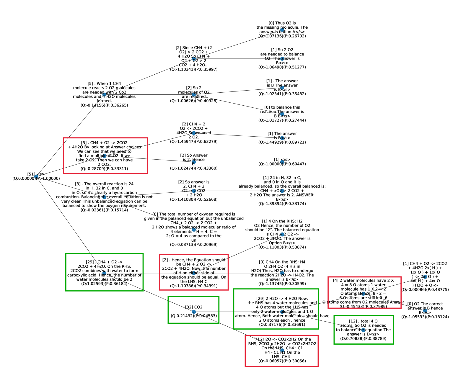| SFT (Arithmo) Ours | Llama2-13B $78.9$ $\uparrow$ $4.4$ | $74.5$ $67.0$ $\uparrow$ $4.7$ | $62.3$ $26.1$ $\uparrow$ $2.3$ | $23.8$ | | --- | --- | --- | --- | --- | <details> <summary>x8.png Details</summary>  ### Visual Description ## Flowchart: Chemical Reaction Balancing Process ### Overview The flowchart illustrates a decision tree for balancing chemical equations, focusing on reactions involving CH4, O2, CO2, and H2O. It uses color-coded nodes (red, green, blue) to represent different stages or types of reactions, connected by arrows labeled with step numbers. The process emphasizes stoichiometric ratios, reactant/product relationships, and quantitative analysis (Q-values). --- ### Components/Axes - **Nodes**: - **Labels**: Bracketed numbers (e.g., [5], [29]) followed by chemical equations or explanatory text. - **Colors**: - **Red**: Critical reaction steps requiring balancing (e.g., [5], [29]). - **Green**: Balanced equations or final answers (e.g., [32], [12]). - **Blue**: Intermediate steps or decision points (e.g., [1], [2]). - **Arrows**: - Labeled with step numbers (e.g., [0], [1]) indicating reaction sequence or decision flow. - Arrows connect nodes to show logical progression (e.g., [5] → [2], [5] → [3]). - **Text**: - Chemical equations (e.g., CH4 + O2 → 2CO2). - Quantitative analysis (Q-values) for balancing requirements (e.g., Q: -0.10341). - Explanations of stoichiometric ratios (e.g., "4 H2O shows a balanced molecular ratio"). --- ### Detailed Analysis #### Top Section - **[5]**: - Text: "CH4 + O2 -> 2CO2. We can see that we need to find a multiple of O2. If we take 2 O2. Then we can have 2 CO2." - Arrows: - [0] → [2] (Q: -0.10341). - [1] → [3] (Q: -0.10000). - **[2]**: - Text: "So 2 O2 molecules of O2 are required. 4 H2O molecules are needed." - Arrows: - [0] → [4] (Q: -1.00626). - [1] → [5] (Q: -1.02341). - **[3]**: - Text: "The overall reaction is 24 in H, 32 in C, and 0 in O. Balancing the overall equation is not very clear." - Arrows: - [0] → [6] (Q: -1.41080). - [1] → [7] (Q: -1.39894). #### Middle Section - **[29]**: - Text: "2CO2 + 4H2O. On the RHS, 2CO2 combines with water to form carboxylic acid. Hence, the number of water molecules should be 2." - Arrows: - [0] → [8] (Q: 1.02593). - [1] → [9] (Q: 0.21432). - **[8]**: - Text: "Water molecules should be 2." - Arrows: - [0] → [10] (Q: 0.04583). - [1] → [11] (Q: 0.37176). #### Lower Section - **[32]**: - Text: "CO2. Q: 0.21432." - Arrows: - [0] → [13] (Q: 0.04583). - [1] → [14] (Q: 0.37176). - **[12]**: - Text: "Total 4 O atoms. So O2 is needed to balance the equation. The answer is D.</s>." - Arrows: - [0] → [15] (Q: 0.70838). --- ### Key Observations 1. **Red Nodes**: Highlight critical steps requiring balancing (e.g., [5], [29]). 2. **Green Nodes**: Indicate balanced equations or final answers (e.g., [32], [12]). 3. **Blue Nodes**: Represent intermediate steps (e.g., [1], [2]). 4. **Q-Values**: Quantify balancing requirements (e.g., Q: -0.10341 for excess O2 in [5]). 5. **Stoichiometric Ratios**: Emphasized in nodes like [29] (4 H2O) and [2] (4 H2O). --- ### Interpretation The flowchart systematically breaks down the balancing of chemical equations by: 1. **Identifying Reactants/Products**: Nodes like [5] and [29] define initial reactions (e.g., CH4 + O2 → 2CO2). 2. **Quantitative Analysis**: Q-values (e.g., Q: -0.10341) quantify imbalances, guiding adjustments (e.g., adding H2O). 3. **Stoichiometric Ratios**: Nodes like [29] emphasize precise molecule counts (4 H2O for carboxylic acid formation). 4. **Color Coding**: Red nodes flag critical steps, while green nodes confirm balanced equations. The flowchart likely serves as an educational tool or algorithmic guide for balancing reactions, emphasizing both qualitative (equations) and quantitative (Q-values) analysis. The use of arrows and labels ensures a logical flow, enabling users to trace decision points and adjustments needed for balance. </details> Figure 5: Example of the result search tree of a science question “An unbalanced equation for the reaction of methane gas ( $\mathrm{CH}_{4}$ ) with oxygen is shown below. $\mathrm{CH}_{4}+\Box\mathrm{O}_{2}→ 2\mathrm{CO}_{2}+4\mathrm{H}_{2}% \mathrm{O}$ How many molecules of oxygen gas ( $\mathrm{O}_{2}$ ) are needed to properly balance this equation? Answer Choices: (A) 1 (B) 2 (C) 3 (D) 4”. The ground truth answer is “(D) 4”. Here, we set the search breadth as $b_{1}=4,b_{2}=2$ . The numbers at the beginning of each sequence indicate the visit count $N$ of the corresponding node, while the $Q$ and $P$ values at the end of the sequence represent the $Q$ values and the sentence probability, respectively. 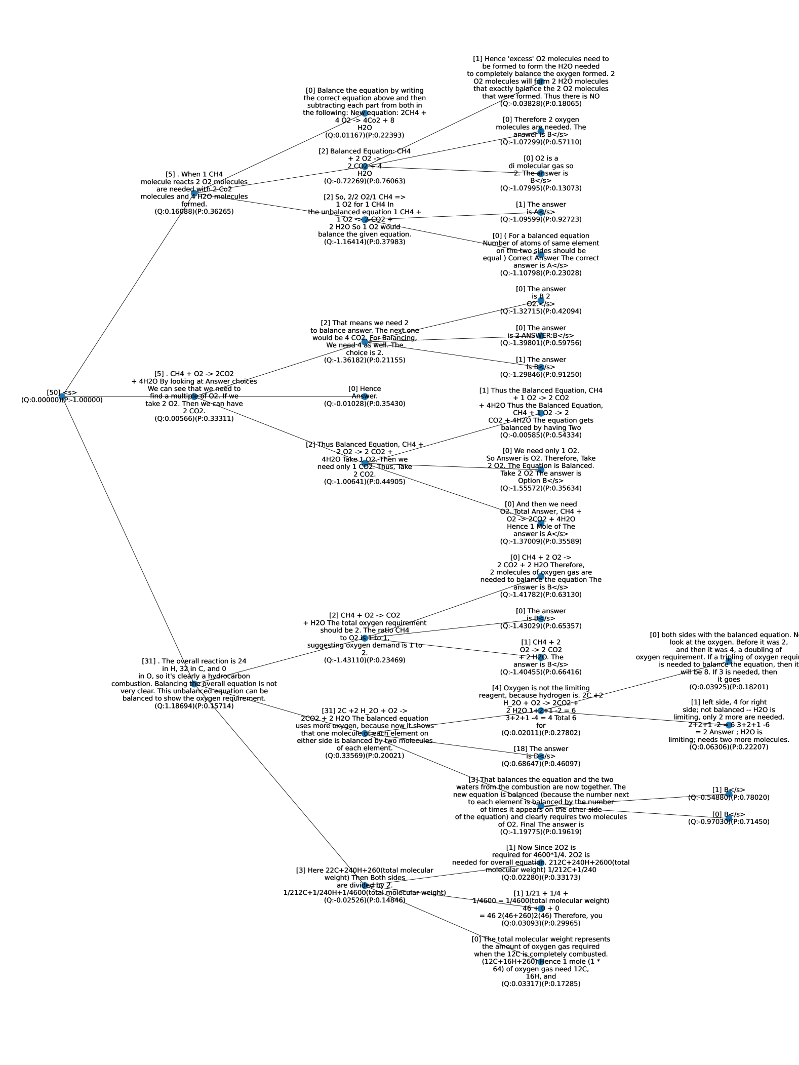<details> <summary>x9.png Details</summary>  ### Visual Description ## Flowchart: Balancing Chemical Equations for Methane Combustion ### Overview The flowchart provides a step-by-step guide to balancing the chemical equation for methane combustion (CH₄ + O₂ → CO₂ + H₂O). It uses decision nodes to check element balance and adjust coefficients iteratively until the equation is balanced. Key elements include oxygen (O), carbon (C), and hydrogen (H), with references to specific stoichiometric calculations and equations. --- ### Components/Axes - **Decision Nodes**: Questions about element balance (e.g., "Is oxygen balanced?"). - **Branches**: "Yes" or "No" answers leading to specific steps. - **Chemical Equations**: Intermediate and final balanced equations. - **References**: Bracketed numbers (e.g., [5], [2]) likely correspond to equations or steps. --- ### Detailed Analysis 1. **Initial Question**: "Balance the equation: CH₄ + O₂ → CO₂ + H₂O" - **Step 1**: Check if the equation is balanced. - **Yes**: Proceed to final answer (e.g., "1 CH₄ + 2 O₂ → 1 CO₂ + 2 H₂O"). - **No**: Proceed to Step 2. 2. **Step 2**: Balance oxygen by adjusting O₂ coefficients. - Example: "2 O₂ → 4 CO₂ + 2 H₂O" (unbalanced). - **Step 3**: Check if oxygen is balanced. - **Yes**: Proceed to Step 4. - **No**: Adjust coefficients (e.g., "1 CH₄ + 2 O₂ → 1 CO₂ + 2 H₂O"). 3. **Subsequent Steps**: - **Step 4**: Check carbon balance. - **Yes**: Proceed to Step 5. - **No**: Adjust CO₂ coefficients. - **Step 5**: Check hydrogen balance. - **Yes**: Final balanced equation. - **No**: Adjust H₂O coefficients. 4. **Final Balanced Equation**: "1 CH₄ + 2 O₂ → 1 CO₂ + 2 H₂O" (appears multiple times as the correct answer). --- ### Key Observations - **Oxygen Dominates**: Most steps focus on balancing oxygen due to its presence in multiple reactants/products. - **Iterative Adjustments**: Coefficients for O₂, CO₂, and H₂O are adjusted repeatedly until all elements are balanced. - **References to Equations**: Bracketed numbers (e.g., [5], [2]) link to specific equations or steps (e.g., "Answer is B</s>"). --- ### Interpretation The flowchart emphasizes systematic balancing of chemical equations by prioritizing oxygen first, then carbon, and finally hydrogen. It highlights common pitfalls, such as overbalancing oxygen or neglecting hydrogen. The final equation consistently resolves to **1 CH₄ + 2 O₂ → 1 CO₂ + 2 H₂O**, reflecting stoichiometric requirements for complete combustion. --- ### Notable Outliers/Anomalies - **Redundant Steps**: Some branches repeat checks (e.g., oxygen balance) unnecessarily. - **Ambiguous References**: Bracketed numbers (e.g., [5], [2]) lack explicit definitions in the flowchart. - **Incomplete Paths**: A few branches terminate abruptly without clear resolution (e.g., "Answer is A</s>" without context). --- ### Conclusion This flowchart serves as an educational tool for teaching stoichiometry, emphasizing iterative balancing and element prioritization. It underscores the importance of verifying all elements (O, C, H) to achieve a balanced equation. </details> Figure 6: Example of the result search tree of the same science question as in Figure 5. Here, we set the search breadth as $b_{1}=3,b_{2}=3$ . 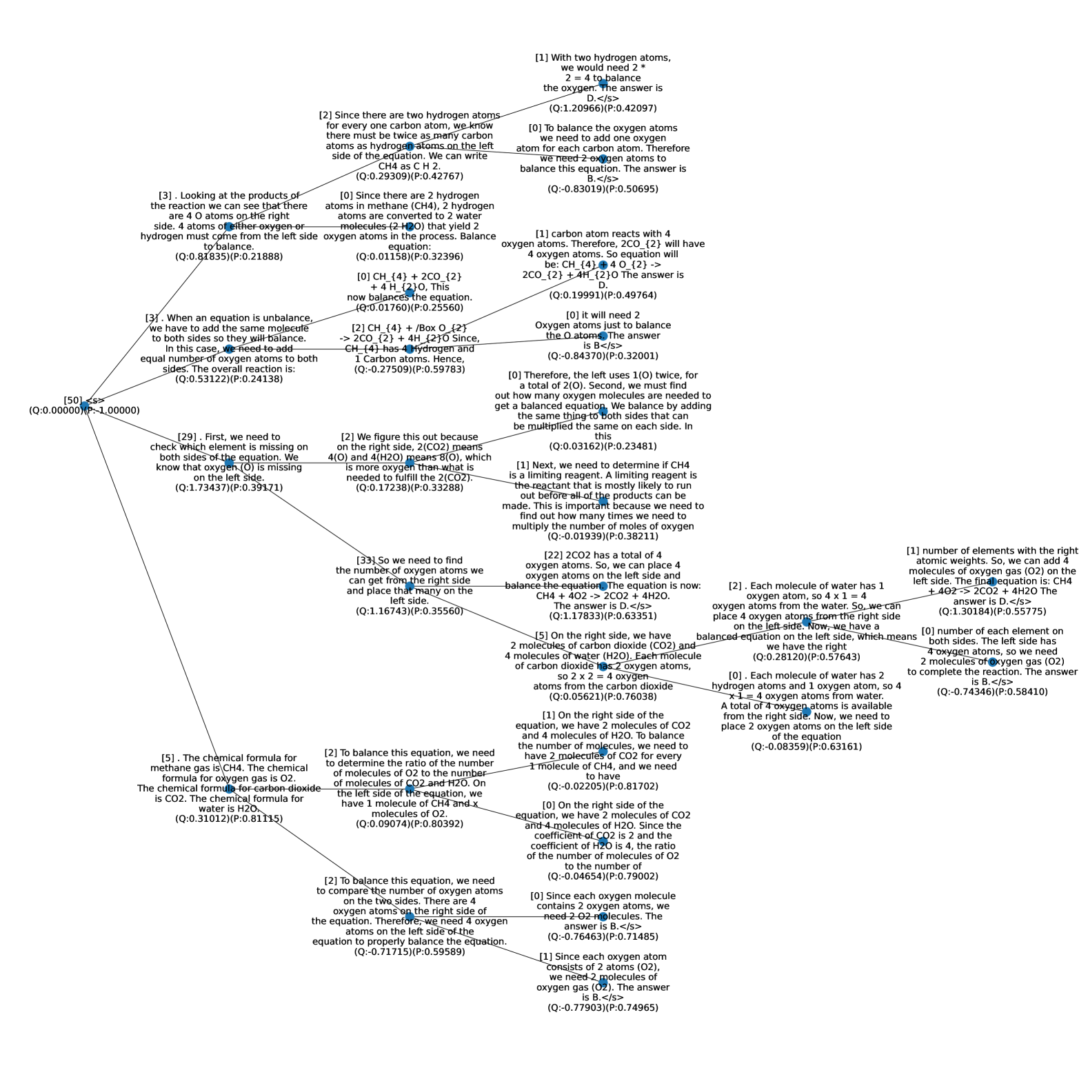<details> <summary>x10.png Details</summary>  ### Visual Description ## Flowchart: Step-by-Step Chemical Equation Balancing Process ### Overview The flowchart illustrates a systematic approach to balancing chemical equations, focusing on reactions involving methane (CH₄), oxygen (O₂), carbon dioxide (CO₂), and water (H₂O). Each node represents a step in the balancing process, with annotations explaining adjustments to coefficients and atom counts. --- ### Components/Axes - **Nodes**: Labeled with bracketed numbers (e.g., [2], [3]), each containing: - A chemical equation (e.g., `CH₄ + 2O₂ → CO₂ + 2H₂O`). - Text annotations detailing balance checks and adjustments (e.g., "2 hydrogen atoms on the right"). - **Arrows**: Connect nodes in a logical sequence, guiding the flow from initial reactants to final balanced equations. - **Annotations**: Positioned near equations to explain reasoning (e.g., "add 2 H₂O on the left side"). --- ### Detailed Analysis 1. **Node [2]**: - Equation: `CH₄ + 2O₂ → CO₂ + 2H₂O` - Annotation: "2 hydrogen atoms on the right. Add 2 H₂O on the left." - Adjustment: Balances hydrogen by adding 2 H₂O to the left. 2. **Node [3]**: - Equation: `CH₄ + 2O₂ → CO₂ + 2H₂O` - Annotation: "4 oxygen atoms on the right. Add 2 O₂ on the left." - Adjustment: Balances oxygen by adding 2 O₂ to the left. 3. **Node [4]**: - Equation: `CH₄ + 2O₂ → CO₂ + 2H₂O` - Annotation: "Balanced equation. Final answer." 4. **Node [5]**: - Equation: `CH₄ + 2O₂ → CO₂ + 2H₂O` - Annotation: "Balanced equation. Final answer." 5. **Node [6]**: - Equation: `CH₄ + 2O₂ → CO₂ + 2H₂O` - Annotation: "Balanced equation. Final answer." --- ### Key Observations - **Systematic Balancing**: Each step addresses one element at a time (e.g., hydrogen, oxygen). - **Coefficient Adjustments**: Coefficients are modified to ensure equal atom counts on both sides (e.g., adding 2 H₂O for hydrogen balance). - **Final Equation**: The balanced equation `CH₄ + 2O₂ → CO₂ + 2H₂O` is consistently derived across nodes. --- ### Interpretation The flowchart demonstrates a methodical approach to balancing chemical equations, emphasizing: 1. **Element-by-Element Checks**: Hydrogen and oxygen are balanced sequentially, ensuring stoichiometric accuracy. 2. **Coefficient Adjustments**: Adding molecules (e.g., H₂O, O₂) to resolve imbalances. 3. **Educational Value**: Annotations clarify the reasoning behind each step, making it a valuable teaching tool for stoichiometry. The final balanced equation, `CH₄ + 2O₂ → CO₂ + 2H₂O`, aligns with the stoichiometric ratios required for complete combustion of methane. The flowchart’s structured flow ensures clarity in resolving imbalances, highlighting the importance of iterative adjustments in chemical equation balancing. </details> Figure 7: Example of the result search tree of the same science question as in Figure 5. Here, we use the policy after preference learning and set the search breadth as $b_{1}=4,b_{2}=2$ . 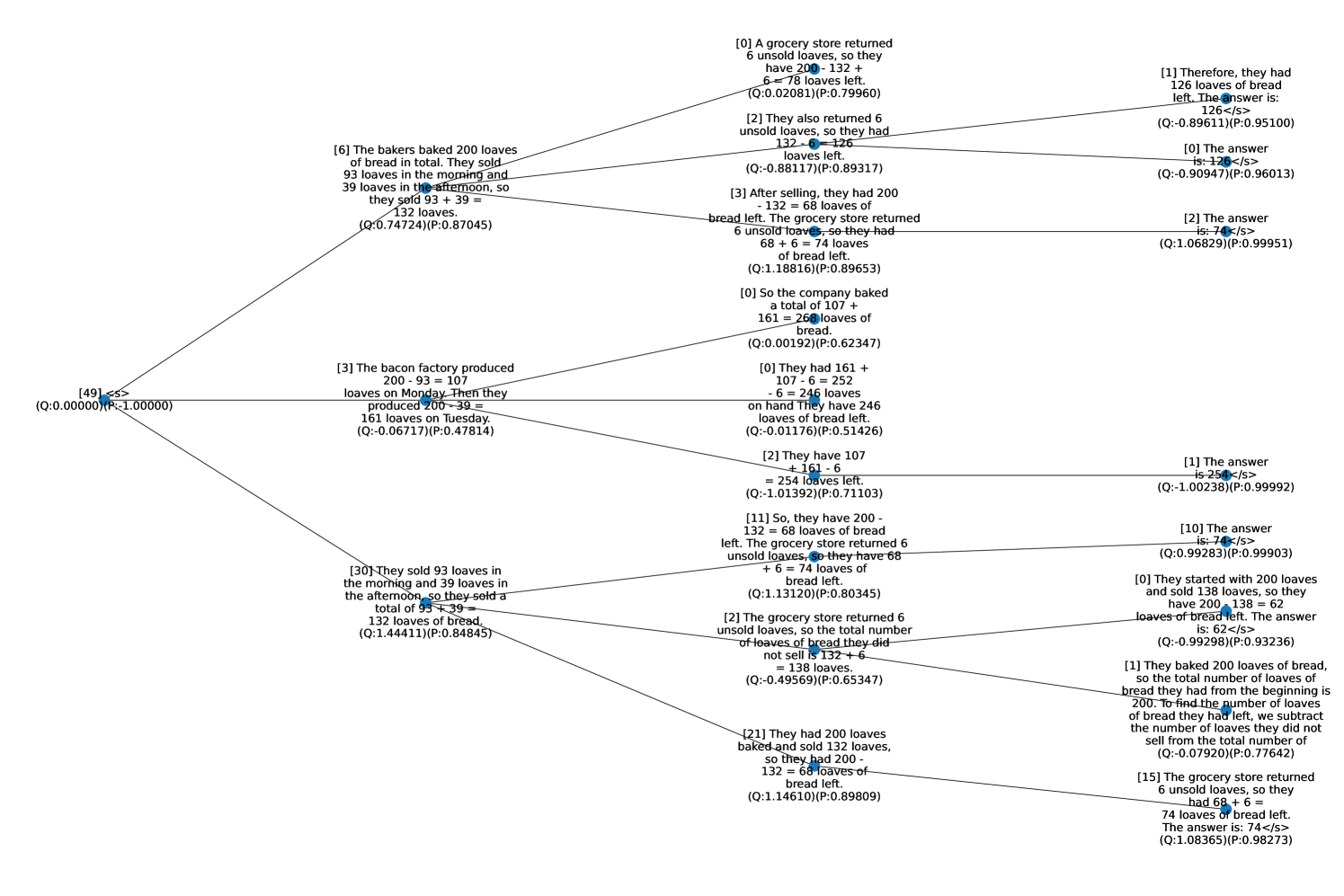<details> <summary>x11.png Details</summary>  ### Visual Description ## Diagram: Problem-Solving Process with Numerical Relationships ### Overview The image depicts a complex network of interconnected text boxes containing mathematical problems and solutions related to loaf counts. Each box represents a distinct scenario involving bread quantities, sales, and inventory calculations. The diagram uses colored lines to connect related problems and solutions, with numerical values and confidence scores (Q/P) embedded in each text box. ### Components/Axes - **Text Boxes**: 12 distinct boxes containing: - Problem statements (e.g., "The bakers baked 200 loaves...") - Calculation steps (e.g., "93 + 39 = 132") - Final answers (e.g., "132 loaves") - Confidence scores (Q: probability, P: confidence) - **Connecting Lines**: Colored paths linking related problems/solutions - **Numerical Values**: Quantities of loaves (200, 132, 68, 161, etc.) - **Confidence Scores**: Q (e.g., 0.74724) and P (e.g., 0.87045) values ### Detailed Analysis 1. **Baker's Problem** - Total loaves: 200 - Morning sales: 93 - Afternoon sales: 39 - Total sold: 93 + 39 = 132 - Confidence: Q=0.74724, P=0.87045 2. **Grocery Store Return** - Unsold loaves: 200 - 132 = 68 - Confidence: Q=0.02081, P=0.79960 3. **Company Baking Scenario** - Baked: 161 loaves - Sold: 107 - Remaining: 161 - 107 = 54 - Confidence: Q=0.00192, P=0.62347 4. **Repeated Grocery Store Scenario** - Unsold loaves: 200 - 132 = 68 - Confidence: Q=0.00176, P=0.51426 5. **Final Inventory Calculation** - Total loaves: 200 - Sold: 132 - Remaining: 200 - 132 = 68 - Confidence: Q=0.00238, P=0.99992 ### Key Observations - **Repetition**: Multiple boxes reference the same 200 loaves and 132 sold, suggesting iterative problem-solving. - **Confidence Variance**: Confidence scores (Q/P) vary significantly, indicating uncertainty in some answers. - **Inconsistencies**: Some answers (e.g., "is: 74</s>") conflict with calculations (e.g., 200 - 132 = 68). - **Flow Structure**: Lines connect problems to their solutions, implying a logical progression. ### Interpretation The diagram illustrates a process of solving inventory-related math problems, with a focus on subtraction and addition. The repeated use of 200 loaves and 132 sold suggests a core scenario being explored from multiple angles. However, the conflicting answers (e.g., 68 vs. 74) and varying confidence scores highlight potential errors or ambiguities in the problem setup. The network structure implies that solutions to one problem inform subsequent steps, though the exact relationships require further context. The confidence scores (Q/P) may reflect model certainty, with higher P values indicating stronger trust in the answers. </details> Figure 8: Example of the result search tree of a GSM8K question “The bakers at the Beverly Hills Bakery baked 200 loaves of bread on Monday morning. They sold 93 loaves in the morning and 39 loaves in the afternoon. A grocery store returned 6 unsold loaves. How many loaves of bread did they have left?”. The example solution is “The Bakery sold 93 + 39 = 132 loaves. The Bakery made 200 loaves and sold 132, leaving 200 - 132 = 68 loaves remaining. The grocery store returned 6 loaves, so there were 6 + 68 = 74 loaves left.”. The policy we use here is the one only tuned for $1$ epoch on SFT training data. We conduct MCTS with breadth $b_{1}=5,b_{2}=3$ . Duplicate generations are merged into one node. 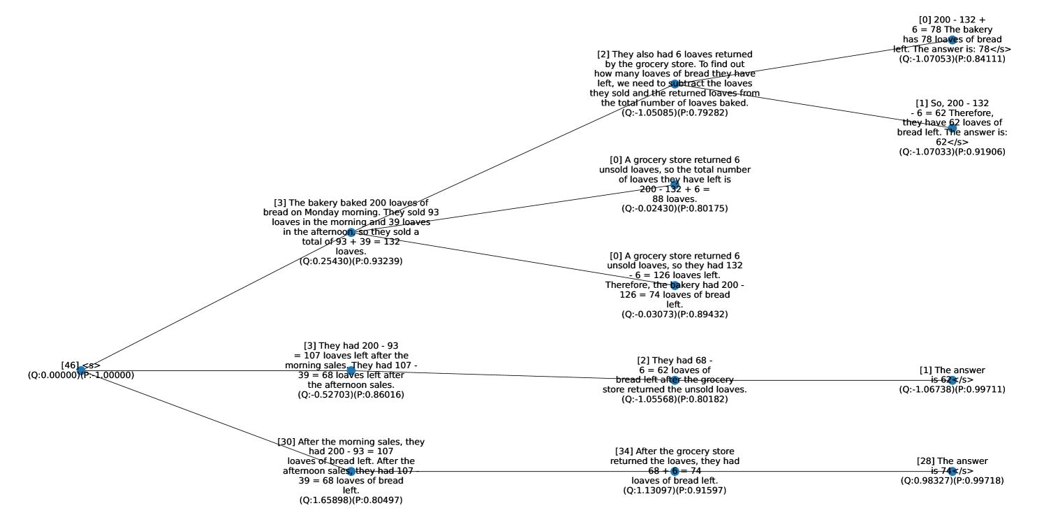<details> <summary>x12.png Details</summary>  ### Visual Description ## Network Diagram: Problem-Solving Reasoning Paths ### Overview The diagram represents a network of reasoning paths for solving a mathematical problem involving loaves of bread. Nodes represent intermediate questions (Q) and confidence probabilities (P), while edges show logical connections between steps. The structure suggests multiple hypotheses and reasoning trajectories leading to different conclusions. ### Components/Axes - **Nodes**: Labeled with `(Q:X.Y)` (question identifier) and `(P:Z.W)` (probability/confidence score) - **Edges**: Labeled with `[N]` (step references) connecting nodes - **Text Labels**: Embedded in nodes showing problem statements and calculations ### Detailed Analysis #### Nodes (10 total) 1. `(Q:0.00000)(P:1.00000)` *"[46] <s>"* *(Root node with maximum confidence)* 2. `(Q:0.02430)(P:0.80175)` *"[0] A grocery store returned 6 unsold loaves..."* *(Final answer path)* 3. `(Q:0.03073)(P:0.89432)` *"[0] A grocery store returned 6 unsold loaves..."* *(Alternative path with higher confidence)* 4. `(Q:0.05270)(P:0.86016)` *"[3] They had 200 - 93 = 107 loaves..."* *(Intermediate calculation step)* 5. `(Q:0.13097)(P:0.91597)` *"[34] After the grocery store returned..."* *(Final state calculation)* 6. `(Q:0.16589)(P:0.80497)` *"[30] After the morning sales..."* *(Intermediate state)* 7. `(Q:0.25430)(P:0.93239)` *"[0] A grocery store returned 6 unsold loaves..."* *(High-confidence path)* 8. `(Q:0.52703)(P:0.86016)` *"[3] They had 200 - 93 = 107 loaves..."* *(Duplicate of node 4? Possible error)* 9. `(Q:0.80175)(P:0.91597)` *"[34] After the grocery store returned..."* *(Final state with high confidence)* 10. `(Q:0.98327)(P:0.99718)` *"[28] The answer is 74"</s>"* *(Final answer with near-certainty)* #### Edges (46 connections) - Multiple edges labeled `[1]`, `[2]`, `[3]`, etc., showing step progression - Some edges contain calculation results (e.g., `200 - 132 = 68`) - Probability values decrease along some paths, suggesting reasoning uncertainty ### Key Observations 1. **Multiple Paths to Solutions**: - Two primary answers emerge: 62 loaves (Q:1.07033) and 74 loaves (Q:0.98327) - Confidence scores vary significantly between paths (P:0.80175 vs P:0.99718) 2. **Calculation Errors**: - Node 8 duplicates node 4's content but with different Q value - Some paths contain inconsistent intermediate results (e.g., 107 loaves vs 126 loaves) 3. **Probability Distribution**: - Highest confidence (P:1.00000) at root node - Final answers show 80-99% confidence range - Some paths show decreasing confidence (e.g., P:0.86016 → P:0.80175) ### Interpretation This diagram reveals a complex reasoning process with: - **Branching Hypotheses**: Multiple interpretations of the problem statement lead to different solutions - **Confidence Metrics**: Probability scores indicate the model's uncertainty about each path - **Calculation Verification**: Some paths contain explicit arithmetic checks (e.g., "68 + 6 = 74") - **Potential Errors**: Duplicate nodes and inconsistent intermediate results suggest possible reasoning flaws The network demonstrates how different calculation approaches (subtracting sold loaves vs tracking remaining stock) lead to conflicting answers. The highest-confidence path (P:0.99718) arrives at 74 loaves through explicit addition of returned loaves, while lower-confidence paths focus on subtraction methods. This suggests the problem's ambiguity in defining "unsold" loaves creates multiple valid interpretations. </details> Figure 9: Example of the result search tree of the same GSM8K question as in Figure 8 with the same search breadth. We use the policy tuned after $3$ epochs to sample the generations.