2405.03917v1

# KV Cache is 1 Bit Per Channel: Efficient Large Language Model Inference with Coupled Quantization **Authors**: Tianyi Zhang, Jonah Yi, Zhaozhuo Xu, Anshumali Shrivastava > Department of Computer Science, Rice University > Department of Computer Science, Stevens Institute of Technology > Department of Computer Science, Rice University ThirdAI Corp. ## Abstract Efficient deployment of Large Language Models (LLMs) requires batching multiple requests together to improve throughput. As the batch size, context length, or model size increases, the size of the key and value (KV) cache can quickly become the main contributor to GPU memory usage and the bottleneck of inference latency. Quantization has emerged as an effective technique for KV cache compression, but existing methods still fail at very low bit widths. We observe that distinct channels of a key/value activation embedding are highly inter-dependent, and the joint entropy of multiple channels grows at a slower rate than the sum of their marginal entropies. Based on this insight, we propose Coupled Quantization (CQ), which couples multiple key/value channels together to exploit their inter-dependency and encode the activations in a more information-efficient manner. Extensive experiments reveal that CQ outperforms or is competitive with existing baselines in preserving model quality. Furthermore, we demonstrate that CQ can preserve model quality with KV cache quantized down to 1-bit. ## 1 Introduction Large Language Models (LLMs) have showcased remarkable generalization abilities across various tasks, including text generation, language translation, and reasoning, without needing specific finetuning [25]. These impressive capabilities have empowered LLMs to find applications in numerous domains, such as law [14], education [15], and patient care [35]. However, the high computational demands and the prohibitive deployment costs of LLMs have created significant barriers, hindering their widespread adoption [14, 3]. Particularly, as LLMs move towards larger model size [9] and longer context length [34], they require faster graphics processing units (GPUs), or other specialized processors, with higher memory capacity for efficient inference. Hence it is crucial to develop approaches for reducing the computational costs and memory requirement of LLMs. To accelerate LLM inference, key and value (KV) caching [20] has been proven to be an effective technique without affecting model quality. In autoregressive decoder-only LLMs, KV caching works through trading off memory for computations: the key and value activations of all previous tokens in the current batch are saved in memory to avoid their recomputation for generating the next token. However, since KV cache scales linearly with the number of tokens and batch size, it can quickly overwhelm the memory capacity of existing GPUs under long context or large batch size settings. In addition, since past key and value activations are not shared between sequences (except for maybe a common prompt), reading the KV cache from GPU memory becomes the primary inference bottleneck as opposed to the computation of the attention scores and value activations of the next token [10]. Thus, it is worthwhile to explore techniques for compressing KV cache for two primary benefits: 1. speeding up LLM inference through reducing the amount of memory reads for KV cache, 2. lowering the GPU memory requirements of inference for a given batch size and context length. Existing approaches typically compress KV cache through token eviction [37, 20] or activation quantization [21, 10]. While they can preserve model quality at moderate compression rates (4 $×$ compression or 4 bits per floating-point number), model quality quickly deteriorates at high compression rates (16 $×$ compression or 1 bit per floating-point number). In this work, we propose Coupled Quantization (CQ), a novel KV cache quantization method that preserves model quality up to 16 $×$ compression or 1 bit per floating-point number. Our approach is motivated by the observation that different channels within the same key/value activation embedding are highly inter-dependent. Thus, it is more information efficient to encode multiple channels of a key/value activation embedding than quantizing each channel independently. Existing KV cache quantization methods employ per-channel or per-token quantization strategies, which fail to exploit the inter-dependence between channels and suffer catastrophic model quality degradation at high compression rates. Our proposed method exploits the mutual dependency between channels by jointly quantizing multiple channels and achieves better preservation of model quality than existing approaches in most cases, especially under low bit width settings. We summarize our contributions as follows, 1. We empirically observe the phenomenon that different channels within the same key/value activation embedding in an LLM share a high amount of dependency or mutual information, which is a key insight not leveraged by existing KV cache compression approaches. 1. We propose Coupled Quantization (CQ), a novel KV cache quantization method that takes advantage of the reduced entropy of jointly encoding multiple channels. 1. Through extensive experiments, we demonstrate the effectiveness of CQ against the most competitive existing methods. Furthermore, we showcase the ability of CQ in preserving model quality at an extreme KV cache compression level of 1-bit. ## 2 Background In this section, we introduce the relevant background and context including the KV caching technique, the von Neumann bottleneck of KV cache, and channel-wise quantization. ### 2.1 LLM Attention and KV Cache Decoder-only transformer-based LLMs employ masked self-attention [32], in which activations of the current token is only dependent on previous tokens and unaffected by future ones. This property enables training parallelism for the next-token prediction objective, and gives rise to the KV caching technique for efficient inference decoding. Consider the decoding step for the $t$ -th token in a single head of attention in an LLM. The input embedding of the $t$ -th token (a column vector), $e_t$ , goes through three distinct transformations to become key, query, and value activation embeddings $f_K(e_t),f_Q(e_t),f_V(e_t)$ , where the transformations $f_K,f_Q,f_V$ are composed of linear projection and positional encoding such as RoPE [29]. The output embedding of attention for the $t$ -th token is computed as $$ attention(e_t)=\biggl{[}\begin{array}[]{ccc}f_V(e_1)&\dots&f_V (e_t)\end{array}\biggr{]}softmax\Biggl{(}\biggl{[}\begin{array}[]{ ccc}f_K(e_1)&\dots&f_K(e_t)\end{array}\biggr{]}^⊤f_Q(e_t) \Biggr{)} \tag{1} $$ Thus, computing the output embedding of the current token requires the key and value activation embeddings of all previous tokens, $f_K(e_i)$ and $f_V(e_i)$ where $i∈≤ft\{1,\dots,t-1\right\}$ . These embeddings are cached in memory from previous decoding steps as KV cache to avoid redundant computations and reduce inference latency. The size of KV cache can be calculated as $b× n× l× 2× h× c$ floating-point numbers, where $b$ is the batch size, $n$ is the number of tokens in each sequence, $l$ is the number of layers in the model, $2$ is for key and value, $h$ is the number of key/value attention heads, and $c$ is the number of channels in a single head of key/value activation embedding. As batch size, context length, or model size increases, the size of KV quickly overwhelms limited GPU memory. ### 2.2 The von Neumann Bottleneck of KV Cache The attention computation in Equation 1 is primarily bottlenecked by GPU memory bandwidth, known as the von Neumann bottleneck, due to low compute-to-global-memory-access ratio. GPUs are able to perform computations significantly faster than reading from global memory, and previous works have shown that attention computation can be accelerated by avoiding unnecessary global memory reads/writes through kernel fusion [5]. During the decoding phase in LLM attention, computing the output for the current token requires fetching the cached key and value embeddings of all previous tokens from global memory, resulting in a low ratio of arithmetic operations to global memory reads [10]. Furthermore, each sequence in a batch retains its own KV cache, leading to poor utilization of the parallel processing capabilities of GPUs. Therefore, KV cache compression algorithms can mitigate the von Neumann bottleneck and improve LLM inference efficiency, even if the approach introduces additional computational overheads in decompression or dequantization. As GPU compute cores are mostly stalled by KV cache memory accesses in attention, quantization approaches can effectively reduce memory reads while introducing negligible latency from dequantization computations. ### 2.3 Channel-wise Quantization Existing KV cache quantization methods [10, 21] employ channel-wise quantization for keys and token-wise quantization for values, based on the observation that certain key channels exhibit outlier patterns in magnitude while value channels do not. Channel-wise and token-wise quantization are similar, except the direction along which the quantization centroids are learned. In non-uniform channel-wise quantization, a set of centroids is learned for each channel. Suppose $A$ is a key or value activation matrix, and $A_i,*$ denotes the $i$ -th channel of $A$ . Then, non-uniform $b$ -bit channel-wise quantization aims to learn a set of centroids $C_i^⋆⊂ℝ$ for each channel $i$ of $A$ independently through the objective $$ C_i^⋆=\operatorname*{arg min}_\begin{subarray{c}C⊂ℝ \\ |C|=2^b\end{subarray}}\Big{\lVert}A_i,*-q(A_i,*)\Big{\rVert}_2^2 \tag{2} $$ where $q$ quantizes each value in $A_i,*$ to the nearest centroid in $C$ . ## 3 Methodology In this section, we motivate our proposal using information theory and introduce the Coupled Quantization (CQ) approach for KV cache compression. <details> <summary>x1.png Details</summary>  ### Visual Description ## Chart/Diagram Type: Layered Entropy Analysis Graphs ### Overview The image contains eight line graphs arranged in a 2x4 grid, each representing entropy metrics across four layers (Layer 1–4). Each layer has two graphs: one for **Key Entropy** (y-axis) and one for **Value Entropy** (y-axis), both plotted against the number of joint channels (x-axis: 1–4). The graphs compare **Sum of Marginal Entropy** (red) and **Joint Entropy** (blue), with trends showing increasing entropy as joint channels increase. ### Components/Axes - **X-axis**: "Num. of Joint Channels" (values: 1, 2, 3, 4) - **Y-axis (Top Row)**: "Key Entropy (bits)" (range: 0–15) - **Y-axis (Bottom Row)**: "Value Entropy (bits)" (range: 0–10) - **Legend**: - Red circles: **Sum of Marginal Entropy** - Blue crosses: **Joint Entropy** - **Graph Titles**: Layer 1 (top-left), Layer 2 (top-center-left), Layer 3 (top-center-right), Layer 4 (top-right), with corresponding Key/Value Entropy graphs below each. ### Detailed Analysis #### Layer 1 - **Key Entropy**: - Sum of Marginal Entropy (red): Starts at ~2 bits (1 joint channel), rises to ~14 bits (4 joint channels). - Joint Entropy (blue): Starts at ~2 bits, rises to ~8 bits. - **Value Entropy**: - Sum of Marginal Entropy (red): Starts at ~2 bits, rises to ~11 bits. - Joint Entropy (blue): Starts at ~2 bits, rises to ~9 bits. #### Layer 2 - **Key Entropy**: - Sum of Marginal Entropy (red): ~2 → ~14 bits. - Joint Entropy (blue): ~2 → ~12 bits. - **Value Entropy**: - Sum of Marginal Entropy (red): ~2 → ~11 bits. - Joint Entropy (blue): ~2 → ~10 bits. #### Layer 3 - **Key Entropy**: - Sum of Marginal Entropy (red): ~2 → ~14 bits. - Joint Entropy (blue): ~2 → ~12 bits. - **Value Entropy**: - Sum of Marginal Entropy (red): ~2 → ~11 bits. - Joint Entropy (blue): ~2 → ~10 bits. #### Layer 4 - **Key Entropy**: - Sum of Marginal Entropy (red): ~2 → ~14 bits. - Joint Entropy (blue): ~2 → ~12 bits. - **Value Entropy**: - Sum of Marginal Entropy (red): ~2 → ~11 bits. - Joint Entropy (blue): ~2 → ~10 bits. ### Key Observations 1. **Consistent Trends**: - Both **Sum of Marginal Entropy** (red) and **Joint Entropy** (blue) increase linearly with the number of joint channels across all layers. - **Sum of Marginal Entropy** consistently exceeds **Joint Entropy** in all layers. 2. **Layer-Specific Patterns**: - Key Entropy graphs (top row) show steeper increases than Value Entropy graphs (bottom row). - Layer 1 has the highest Key Entropy values, while Layer 4 has the lowest Key Entropy values. 3. **Data Point Accuracy**: - Red data points (Sum of Marginal Entropy) are always above blue points (Joint Entropy) in every graph. ### Interpretation - **Entropy Relationships**: - The **Sum of Marginal Entropy** (red) represents the total entropy when joint channels are considered independently, while **Joint Entropy** (blue) reflects entropy when channels are analyzed together. The red line’s dominance suggests that marginal contributions dominate over joint effects. - **Layer Functionality**: - Key Entropy (top row) likely corresponds to critical features or decision boundaries, while Value Entropy (bottom row) may relate to auxiliary or contextual information. The decline in Key Entropy from Layer 1 to Layer 4 implies a shift from high-dimensional decision-making to more streamlined processing. - **Practical Implications**: - The linear relationship between joint channels and entropy indicates that adding channels proportionally increases system complexity. This could inform optimization strategies for neural networks or information compression algorithms. ### Spatial Grounding - **Legend**: Top-right corner, clearly associating red with Sum of Marginal Entropy and blue with Joint Entropy. - **Graph Layout**: Each layer’s graphs are stacked vertically (Key Entropy above Value Entropy), with layers ordered left-to-right (Layer 1–4). - **Axis Consistency**: X-axis labels and scales are uniform across all graphs, ensuring comparability. ### Content Details - **Numerical Values**: - All graphs start at ~2 bits for 1 joint channel, with incremental increases (e.g., Layer 1 Key Entropy: +1 bit per channel). - Final values at 4 joint channels: Key Entropy ~14 bits, Value Entropy ~11 bits. - **Trend Verification**: - Red lines (Sum of Marginal Entropy) slope upward more steeply than blue lines (Joint Entropy) in all layers. ### Final Notes The data underscores the trade-off between marginal and joint entropy in layered systems, with implications for understanding information flow and redundancy in hierarchical models. The consistent patterns suggest a designed relationship between channel count and entropy, potentially reflecting architectural constraints or optimization goals. 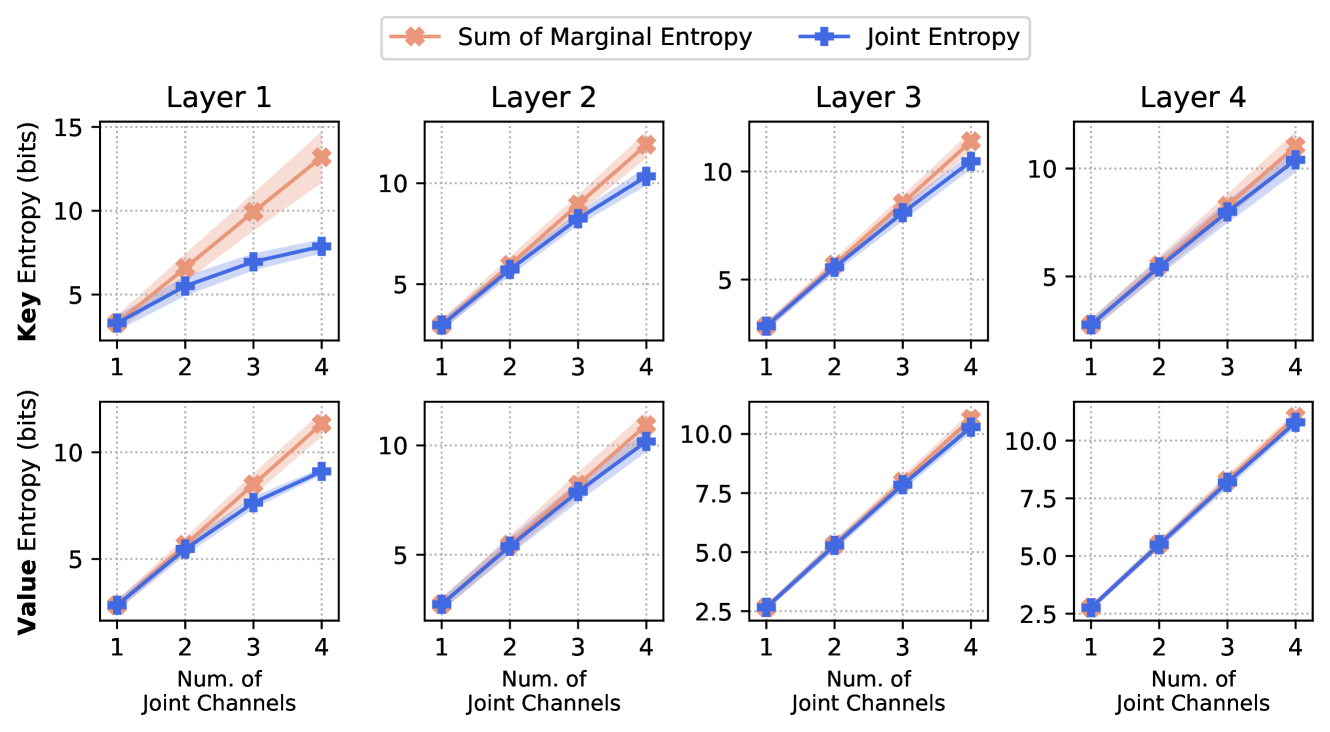</details> Figure 1: Growth rate of joint entropy versus sum of marginal entropies of the LLaMA-7b key/value activation embeddings on 262k tokens of WikiText-2. Entropy is estimated using Equation 4. The slower growth rate of joint entropy implies that jointly quantizing more channels requires fewer bits than quantizing each channel independently. <details> <summary>x2.png Details</summary>  ### Visual Description ## Heatmap: LLaMA-7b Channel-Key and Channel-Value Correlation Patterns Across Layers ### Overview The image presents two sets of heatmaps comparing correlation patterns between channels and keys/values across 8 layers of the LLaMA-7b neural network architecture. The top row shows "Key" correlations, while the bottom row shows "Value" correlations. Each heatmap visualizes 321 channels against 16 key/value dimensions across layers 1, 2, 13, 14, 28, 29, 31, and 32. ### Components/Axes - **X-axis**: Channels (1 to 321) - **Y-axis**: Correlations (1 to 32) - **Legend**: Color scale from -1.0 (blue) to 1.0 (red), with 0.0 as white - **Layer labels**: Positioned above each heatmap column (Layer 1, 2, 13, 14, 28, 29, 31, 32) - **Diagonal reference**: Red dashed line indicating perfect correlation (1.0) ### Detailed Analysis **Key Correlations (Top Row):** - **Layer 1**: Strong block structure with alternating red/blue squares (ranging from -0.8 to 0.8) - **Layer 2**: Similar block pattern but with reduced intensity (ranging from -0.6 to 0.6) - **Layer 13**: Emerging diagonal patterns with moderate correlation strength (ranging from -0.4 to 0.4) - **Layer 14**: More diffuse pattern with scattered red/blue patches (ranging from -0.3 to 0.3) - **Layer 28**: Weak correlation structure with mostly white areas (ranging from -0.2 to 0.2) - **Layer 29**: Further diffusion with minimal correlation patterns (ranging from -0.1 to 0.1) - **Layer 31**: Near-uniform white with faint diagonal traces (ranging from -0.05 to 0.05) - **Layer 32**: Almost entirely white with only residual red/blue spots (ranging from -0.01 to 0.01) **Value Correlations (Bottom Row):** - **Layer 1**: Similar block structure to Key correlations but with slightly reduced intensity (ranging from -0.7 to 0.7) - **Layer 2**: Maintains block pattern with comparable strength to Layer 1 (ranging from -0.6 to 0.6) - **Layer 13**: Shows emerging diagonal patterns with moderate strength (ranging from -0.4 to 0.4) - **Layer 14**: More diffuse pattern with scattered patches (ranging from -0.3 to 0.3) - **Layer 28**: Weak correlation structure with mostly white areas (ranging from -0.2 to 0.2) - **Layer 29**: Further diffusion with minimal patterns (ranging from -0.1 to 0.1) - **Layer 31**: Near-uniform white with faint traces (ranging from -0.05 to 0.05) - **Layer 32**: Almost entirely white with residual spots (ranging from -0.01 to 0.01) ### Key Observations 1. **Diagonal Dominance**: All heatmaps show perfect correlation (1.0) along the diagonal, confirmed by consistent red dashed lines 2. **Layer Evolution**: Early layers (1-2) show strong structured patterns that progressively diffuse through later layers 3. **Key vs Value**: Key correlations maintain stronger structural patterns than Value correlations across all layers 4. **Layer 32 Anomaly**: Both Key and Value correlations approach near-zero values, suggesting minimal channel interactions in final layers 5. **Color Consistency**: Red (positive) and blue (negative) correlations maintain consistent positioning relative to the diagonal across all layers ### Interpretation The data demonstrates a clear progression from structured, task-specific representations in early layers to more generalized, abstract representations in later layers. The strong block patterns in Layer 1 suggest initial attention mechanisms focus on specific channel relationships, while the diffusion in deeper layers indicates increasing model capacity to handle complex, multi-dimensional interactions. The near-zero correlations in Layer 32 imply that final representations have largely disentangled channel dependencies, potentially optimizing for generalization. The consistent diagonal dominance across all layers confirms the expected perfect self-correlation property of attention mechanisms. 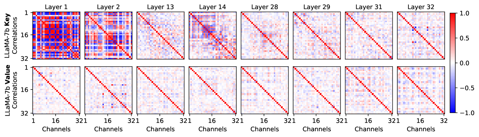</details> Figure 2: Correlation matrices of the first 32 channels of 8 layers of LLaMA-7b key and value activation embeddings on WikiText-2. Channel pairs exhibit high levels of linear dependency, shown by high magnitudes of the correlation coefficients. ### 3.1 Motivations Our proposed approach is inspired by concepts in information theory [28]. We consider each channel in a key/value activation embedding as a random variable $X_1,X_2,\dots$ . The amount of information (or uncertainty) in channel $X$ can be measured by entropy, defined as $H(X)=-∫_Xp(x)\log_2p(x) dx$ , where $p(·)$ is the probability density function and $X$ is the support of $X$ . $H(X)$ measures the theoretical number of bits needed for losslessly encoding the channel $X$ , so it can be used to gauge how “quantizable” a channel is: if $H(X_1)<H(X_2)$ , then channel $X_1$ may be quantized to fewer bits than channel $X_2$ while achieving the same quantization error. Our insight is that different channels from the same key/value activation embedding may be interdependent, which would reduce the number of bits required for jointly encoding multiple channels together compared to encoding them independently. The total amount of information (or uncertainty) in two channels $X_1,X_2$ is measured by joint entropy, defined as $H(X_1,X_2)=-∫_X_1∫_X_2p(x_1,x_2)\log_ 2p(x_1,x_2) dx_2 dx_1$ , where $p(·,·)$ is the joint probability density function. The joint entropy of two channels is the difference between the sum of their marginal entropies and their mutual information, i.e., $H(X_1,X_2)=H(X_1)+H(X_2)-I(X_1,X_2)$ , where $I(·,·)$ is a non-negative quantity for measuring the mutual dependency of two random variables. Thus, we have $$ H(X_1,X_2)≤ H(X_1)+H(X_2) \tag{3} $$ which implies the number of bits needed for jointly encoding two channels is no more than the total number of bits needed for encoding them independently. Previous works have demonstrated that deep neural networks [11] and attention-based networks [7] tend to produce low-rank embeddings, which suggests that channels of key/value embedding in LLM may exhibit high amount of mutual dependency. It is hence beneficial to measure the difference between the joint entropy of multiple channels and the sum of their marginal entropies in key and value activation embeddings. A significant difference would suggest that encoding these channels together is more information-efficient than encoding them independently. However, it is intractable to derive the exact entropy or joint entropy of channels, since their probability density functions are not known. Therefore, we employ the “binning” trick [17] to estimate entropy. We first observe an empirical distribution of key and value channels by saving the KV cache on a dataset, and partition the support of each channel into equally sized bins. Then, values of each channel are discretized to the index of the bin they fall into. Finally, the joint entropy of $n$ channels $X_1,\dots,X_n$ is estimated with the Riemann sum, $$ H(X_1,\dots,X_n)≈∑_x_{1∈B_1}\dots∑_x_{n∈ B_n}\widehat{p}(x_1,\dots,x_n)\log_2\widehat{p}(x_1,\dots,x _n) \tag{4} $$ where $B_i$ is the support of the binned or discretized $X_i$ and $\widehat{p}(·)$ is the empirical probability density function. Specifically, we divide the channels of key and value embeddings of LLaMA-7b into non-overlapping groups of $c$ contiguous channels, where $c∈\{1,2,3,4\}$ , and estimate the joint entropy and the sum of marginal entropies of each group. The support of each channel is partitioned into 16 equally sized bins. Figure 1 shows the mean and standard deviation of the estimated joint entropy and sum of marginal entropies of three layers of LLaMA-7b on 262k tokens of the WikiText-2 dataset, averaged over groups. We only show a maximum group size of 4, since increasing the group size requires saving exponentially more key and value embeddings to avoid empty bins and maintain estimation quality. As shown in Figure 1, the sum of marginal entropies grows at a linear rate while the joint entropy increases slower at a sub-linear rate. This implies that as the number of jointly quantized channels increases, the total amount of information needed for encoding decreases. This phenomenon is the foundation that motivates our proposed approach. 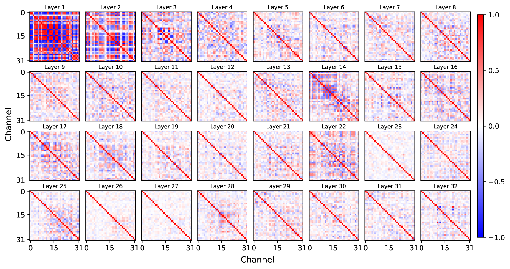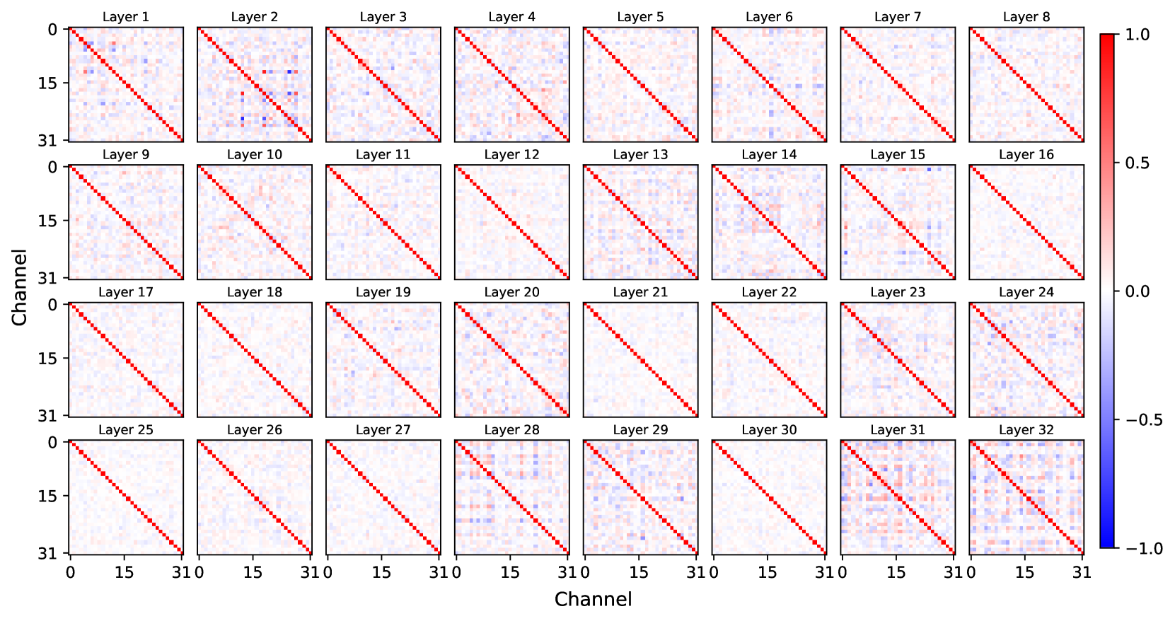In addition to presenting the estimated marginal and joint entropy, we also show the Pearson correlation coefficients between channels of LLaMA-7b key and value activation embeddings on WikiText-2. Correlation coefficient captures the linear dependency between two random variables. Heat maps for the correlation matrices of 8 layers are shown in Figure 2, while the correlation matrices of all layers are presented in Section Appendix of the Appendix. The key and value channels exhibit high levels of linear dependency and they are clearly not independently distributed, as shown by high magnitudes of the correlation coefficients. <details> <summary>x3.png Details</summary>  ### Visual Description ## Diagram: Channel-wise and Coupled Quantization Techniques ### Overview The image compares two quantization methods: **Channel-wise Quantization** (left) and **Coupled Quantization** (right). Each section includes a diagram of activation embedding and centroids, along with a scatter plot showing original (blue "+") and quantized (red "×") values. Quantization errors are explicitly labeled for both methods. --- ### Components/Axes #### Left Section: Channel-wise Quantization - **Diagram Labels**: - "key or value activation embedding" (input) - "channel-wise centroids" (output) - Channels: 0, 1, ... (vertical axis) - Centroid values: - Channel 0: `q₀ = [-0.57, 0.21]` - Channel 1: `q₁ = [-0.38, -0.13]` - Quantization error: `601.4` (red text) - **Scatter Plot**: - **Axes**: - X-axis: "channel 0" (range: -0.8 to 0.4) - Y-axis: "channel 1" (range: -0.4 to 0.0) - **Legend**: - Blue "+": original values - Red "×": quantized values - Dashed lines: channel-wise centroids #### Right Section: Coupled Quantization - **Diagram Labels**: - "coupled channels 0 & 1" (input) - "multi-channel centroids" (output) - Centroid values: - `[-0.62, 0.11, 0.30, -0.38, -0.10, -0.13, -0.24]` - Quantization error: `250.6` (green text) - **Scatter Plot**: - **Axes**: - X-axis: "channel 0" (range: -0.8 to 0.4) - Y-axis: "channel 1" (range: -0.4 to 0.0) - **Legend**: - Blue "+": original values - Red "×": quantized values --- ### Detailed Analysis #### Channel-wise Quantization - **Centroids**: - Channel 0: Two centroids at `(-0.57, 0.21)` and `(0, 1)`. - Channel 1: Two centroids at `(-0.38, -0.13)` and `(0, 1)`. - **Quantization Error**: `601.4` (high error, indicating poor approximation). - **Scatter Plot Trends**: - Original values (blue "+") form a curved distribution. - Quantized values (red "×") cluster near centroids, with significant deviation from original data. #### Coupled Quantization - **Centroids**: - Seven centroids across channels 0 and 1 (e.g., `(-0.62, 0.11, 0.30, ...)`). - **Quantization Error**: `250.6` (lower error than channel-wise, suggesting better approximation). - **Scatter Plot Trends**: - Original values (blue "+") show similar curvature. - Quantized values (red "×") align more closely with centroids, reducing deviation. --- ### Key Observations 1. **Quantization Error Reduction**: - Coupled Quantization (`250.6`) achieves a **58% reduction** in error compared to Channel-wise (`601.4`). 2. **Centroid Distribution**: - Channel-wise uses per-channel centroids, while Coupled uses multi-channel centroids, enabling finer granularity. 3. **Data Point Alignment**: - In Coupled Quantization, quantized values (red "×") are closer to original values (blue "+") than in Channel-wise. --- ### Interpretation - **Technical Insight**: - Coupled Quantization improves accuracy by modeling inter-channel dependencies, whereas Channel-wise treats channels independently. - **Practical Implications**: - Lower quantization error in Coupled suggests better preservation of original data, critical for applications like neural networks where precision matters. - **Anomalies**: - No outliers in the scatter plots, but the centroid placement in Channel-wise (e.g., `(0, 1)`) may not align with data distribution, contributing to higher error. 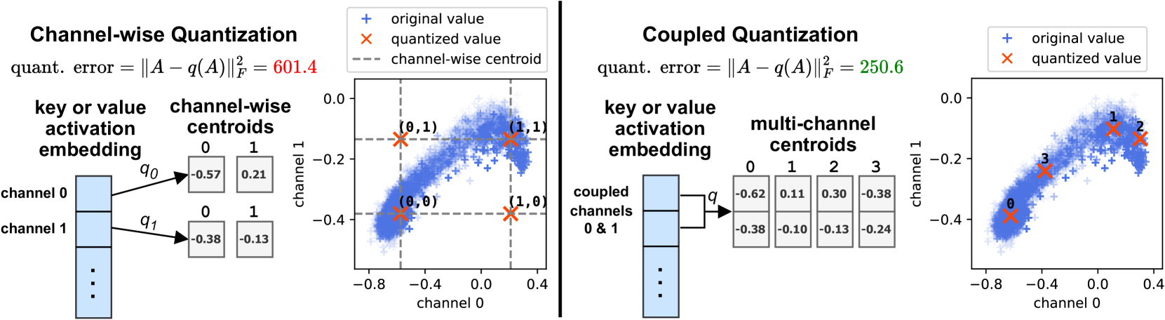</details> Figure 3: A comparison of 1-bit channel-wise quantization and our proposed Coupled Quantization (using 2 bits per 2 channels as an example). The quantization results on the first two channels of the first-layer key activation embeddings of LLaMA-7b on the WikiText-2 dataset are shown. Channel-wise quantization is ineffective at capturing the original values at low widths, while CQ leverages the dependency between channels to achieve low quantization errors. ### 3.2 Coupled Quantization Motivated by the finding that distinct key/value channels exhibit high dependency, we propose Coupled Quantization (CQ), an information-efficient quantization approach for compressing LLM KV cache. Unlike existing KV cache quantization methods which quantizes channel-wise or token-wise, CQ performs channel-coupled quantization for keys and values. More concretely, channels of a key or value activation embedding are divided into equally sized, non-overlapping groups of contiguous channels. The channels in each group are coupled, as they are jointly quantized and share a single quantization code. For each group of coupled channels, a distinct set of multi-channel centroids are learned, where each centroid has dimensionality equal to the number of channels in that group. When quantizing a key or value activation embedding, each group of coupled channels are quantized to the nearest centroid in terms of L2 distance. We use the CQ- <c> c <b> b notation to denote the configuration of channel coupling and quantization bit width, where <c> is the number of channels in each group and <b> indicates the number of bits in a quantized code for a group. For example, CQ-4c8b means that every 4 contiguous channels are coupled together and each coupled group shares an 8-bit code, which is equivalent to 2-bit channel-wise quantization in terms of storage overhead of quantized codes. A illustrative comparison of channel-wise quantization and CQ is shown in Figure 3. Although previous works [10, 21] opt to quantize keys channel-wise and values token-wise, we adopt channel-coupled quantization for both keys and values. Similar to existing approaches [10, 21], CQ quantizes keys before RoPE [29] is applied, which increases the quantization difficulty by introducing more outliers in key activations. <details> <summary>x4.png Details</summary>  ### Visual Description ## Line Charts: LLaMA-7b CQ Configurations on WikiText-2 ### Overview The image contains four line charts comparing the performance of different CQ (Contextual Quantization) configurations on the LLaMA-7b model using WikiText-2. Each chart evaluates metrics like **perplexity** and **quantization error** across varying CQ configurations (1c1b, 2c2b, 4c4b, 8c8b). The charts use logarithmic and linear scales to visualize trends. --- ### Components/Axes 1. **X-Axes (CQ Config.)**: - Labels: `1c1b`, `2c2b`, `4c4b`, `8c8b` (context window size and quantization bits). 2. **Y-Axes**: - **Left Y-Axis (Perplexity on WikiText-2)**: Logarithmic scale (10¹ to 10³). - **Right Y-Axes (Quant. Error on WikiText-2)**: Linear scale (500 to 2000). 3. **Legends**: - **Uniform CQ**: Orange lines/triangles. - **Fisher-guided CQ**: Green lines/triangles. - **FP16 Baseline**: Gray dashed line (constant value). --- ### Detailed Analysis #### Chart 1: LLaMA-7b 1-bit CQ (Perplexity) - **Trend**: - Uniform CQ (orange) slopes steeply downward from **2642.72** (1c1b) to **32.12** (8c8b). - Fisher-guided CQ (green) slopes less steeply from **620.08** (1c1b) to **8.09** (8c8b). - FP16 Baseline (gray) remains constant at **5.68**. - **Data Points**: - Uniform CQ: `1c1b` (2642.72), `2c2b` (1614.02), `4c4b` (883.60), `8c8b` (32.12). - Fisher-guided CQ: `1c1b` (620.08), `2c2b` (28.39), `4c4b` (10.47), `8c8b` (8.09). #### Chart 2: LLaMA-7b 2-bit CQ (Perplexity) - **Trend**: - Uniform CQ (orange) slopes downward from **204.56** (1c1b) to **6.86** (8c8b). - Fisher-guided CQ (green) slopes slightly from **6.37** (1c1b) to **5.97** (8c8b). - FP16 Baseline (gray) remains at **5.68**. - **Data Points**: - Uniform CQ: `1c1b` (204.56), `2c2b` (24.46), `4c4b` (6.86), `8c8b` (5.97). - Fisher-guided CQ: `1c1b` (6.37), `2c2b` (6.08), `4c4b` (6.08), `8c8b` (5.97). #### Chart 3: LLaMA-7b 1-bit CQ (Quant. Error) - **Trend**: - Uniform CQ Key (orange) slopes from **1750** (1c1b) to **750** (8c8b). - Fisher-guided CQ Key (green) slopes from **1750** (1c1b) to **600** (8c8b). - Uniform CQ Value (orange triangle) slopes from **750** (1c1b) to **500** (8c8b). - Fisher-guided CQ Value (green triangle) slopes from **750** (1c1b) to **500** (8c8b). - **Data Points**: - Uniform CQ Key: `1c1b` (1750), `2c2b` (1500), `4c4b` (1250), `8c8b` (750). - Fisher-guided CQ Key: `1c1b` (1750), `2c2b` (1500), `4c4b` (1250), `8c8b` (600). - Uniform CQ Value: `1c1b` (750), `2c2b` (600), `4c4b` (500), `8c8b` (500). - Fisher-guided CQ Value: `1c1b` (750), `2c2b` (600), `4c4b` (500), `8c8b` (500). #### Chart 4: LLaMA-7b 2-bit CQ (Quant. Error) - **Trend**: - Uniform CQ Key (orange) slopes from **1000** (1c1b) to **600** (8c8b). - Fisher-guided CQ Key (green) slopes from **1000** (1c1b) to **600** (8c8b). - Uniform CQ Value (orange triangle) slopes from **800** (1c1b) to **400** (8c8b). - Fisher-guided CQ Value (green triangle) slopes from **800** (1c1b) to **400** (8c8b). - **Data Points**: - Uniform CQ Key: `1c1b` (1000), `2c2b` (800), `4c4b` (600), `8c8b` (600). - Fisher-guided CQ Key: `1c1b` (1000), `2c2b` (800), `4c4b` (600), `8c8b` (600). - Uniform CQ Value: `1c1b` (800), `2c2b` (600), `4c4b` (400), `8c8b` (400). - Fisher-guided CQ Value: `1c1b` (800), `2c2b` (600), `4c4b` (400), `8c8b` (400). --- ### Key Observations 1. **Perplexity Reduction**: - Both CQ methods reduce perplexity as CQ configuration increases (e.g., 1c1b → 8c8b). - Fisher-guided CQ consistently outperforms Uniform CQ (e.g., 620.08 vs. 2642.72 in 1c1b for perplexity). 2. **Quantization Error**: - Fisher-guided CQ reduces error more effectively than Uniform CQ (e.g., 600 vs. 750 in 8c8b for 1-bit CQ). - 2-bit CQ configurations show smaller error reductions compared to 1-bit. 3. **FP16 Baseline**: - Acts as a lower bound for perplexity (5.68) but does not affect quantization error. --- ### Interpretation - **Fisher-guided CQ** demonstrates superior performance in both perplexity and quantization error across all configurations, suggesting it better preserves model quality during quantization. - **Uniform CQ** shows significant improvement with larger CQ configurations but remains less efficient than Fisher-guided CQ. - The **FP16 Baseline** highlights the trade-off between quantization and model fidelity, as CQ methods achieve lower perplexity than FP16 while maintaining competitive quantization error. - The logarithmic scale for perplexity emphasizes the exponential reduction in error with increased CQ bits, critical for low-resource deployment scenarios. 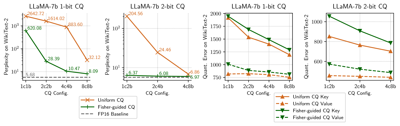</details> Figure 4: Perplexity and key/value quantization errors (averaged over all layers) of LLaMA-7b on WikiText-2. Channels coupling and Fisher-guided centroid learning are effective for improving perplexity. #### 3.2.1 Centroid Learning In CQ, the multi-channel centroids for each channel group are learned offline on a calibration dataset by leveraging uniform clustering or second-order-information-informed clustering. Specifically, for uniform centroid learning of the CQ- $c$ c $b$ b configuration, a set of centroids $C_i^⋆⊂ℝ^c$ is learned independently for each channel group $i$ through the objective $$ C_i^⋆=\operatorname*{arg min}_\begin{subarray{c}C∈ℝ^c \\ ≤ft|C\right|=2^b\end{subarray}}\Big{\lVert}A_ic:(ic+c-1), *- \operatorname*{cq}\big{(}A_ic:(ic+c-1), *\big{)}\Big{\rVert}^2_F \tag{5} $$ where $A_ic:(ic+c-1), *$ is the sub-matrix of $A$ containing all coupled channels of the $i$ -th group, and $\operatorname*{cq}$ quantizes each column vector to the nearest centroid in $C$ in terms of L2 distance. We use the k-means algorithm [22] with k-means++ initialization [1] to optimize the objective. LLMs are more sensitive to the quantization precision of certain weights than others [16]. To better preserve model quality, centroids of CQ should be learned to be biased towards preserving the precision of more important activations. To this end, we leverage an approximation to the Hessian to perform second-order-information-informed centroid learning. More concretely, we use the diagonals of the Fisher information matrix $F$ to identify the more influential key/value activations and guide the centroid learning process. This method was proposed by Li et al. [18] and used by Kim et al. [16] for channel-wise weight quantization, and we extend it to multi-channel CQ. For performing Fisher-guided centroid learning, we first save a key/value activation matrix $A$ and its gradient $g(A)=\frac{∂}{∂ A}L(A)$ on a calibration dataset, where $L$ is the training loss function. We approximate the Hessian matrix using the diagonals of the Fisher information matrix, which is the element-wise square of the gradient matrix $diag(F)=g(A)\odot g(A)$ . We use the sum of diagonal entries of the Fisher information matrix as a measure of importance for each group of channel-coupled activations, and obtain the centroid set $C_i^⋆$ for the $i$ -th channel group using the objective $$ C_i^⋆=\operatorname*{arg min}_\begin{subarray{c}C⊂ℝ^c\\ ≤ft|C\right|=2^b\end{subarray}}∑_jg\big{(}A_ic:(ic+c-1), j\big{)}^⊤g\big{(}A_ic:(ic+c-1), j\big{)}\Big{\lVert}A_ic:(ic+c-1), j- \operatorname*{cq}(A_ic:(ic+c-1), j)\Big{\rVert}^2_F \tag{6} $$ We leverage weighted k-means to optimize the objective. The overhead of the centroid learning process and centroid storage are discussed in Section 4.3. We validate the effectiveness of our proposed channel-coupling and Fisher-guided centroid learning by compressing LLaMA-7b KV cache to 1-bit and 2-bit, and present the perplexity results and quantization errors ( $\lVert A-\operatorname*{cq}(A)\rVert^2_F$ averaged over layers) on WikiText-2 under different CQ configurations in Figure 4. The experimental setup is given in Section 4. As the number of coupled channels increases, perplexity and quantization errors improve significantly, approaching the FP16 baseline performance. Although Fisher-guided centroid learning increases the quantization error, it better preserves the salient activations and achieve lower perplexity. Table 1: Perplexity on WikiText-2 under different KV cache quantization methods at varying bit-width. The results of INT, NF, and KVQuant (excluding 1b and 1b-1%) are from [10]. “NaN” means Not a Number, which is caused by numerical stability issues of quantization. Our method CQ consistently outperforms non-dense-and-sparse quantization methods, and performs better or on par with the dense-and-sparse method KVQuant- <b> b-1%. | | Bits Per FPN | LLaMA-7b | LLaMA-13b | LLaMA-2-7b | LLaMA-2-13b | Mistral-7b | | --- | --- | --- | --- | --- | --- | --- | | FP16 | 16 | 5.68 | 5.09 | 5.12 | 4.57 | 4.76 | | INT4 | 4.00-4.01 | 5.98 | 5.32 | 5.66 | 5.01 | 4.97 | | INT4-gs128 | 4.16 | 5.77 | 5.16 | 5.32 | 4.71 | 4.82 | | NF4 | 4.00-4.01 | 5.87 | 5.23 | 5.47 | 4.90 | 4.91 | | NF4-gs128 | 4.16 | 5.77 | 5.17 | 5.30 | 4.71 | 4.83 | | KVQuant-4b | 4.00-4.02 | 5.73 | 5.15 | 5.18 | 4.63 | 4.81 | | KVQuant-4b-1% | 4.32-4.35 | 5.70 | 5.11 | 5.14 | 4.59 | 4.78 | | CQ-2c8b | 4.00 | 5.70 | 5.11 | 5.14 | 4.59 | 4.79 | | INT2 | 2.00-2.01 | 11779 | 69965 | 4708 | 3942 | 573 | | INT2-gs128 | 2.14 | 37.37 | 41.77 | 117.88 | 93.09 | 51.96 | | NF2 | 2.00-2.02 | 3210.5 | 5785.6 | 13601 | 4035.6 | 902.51 | | NF2-gs128 | 2.14 | 351.23 | 141.19 | 634.59 | 642.44 | 252.85 | | KVQuant-2b | 2.00-2.02 | 8.17 | 7.29 | 9.75 | 29.25 | 7.33 | | KVQuant-2b-1% | 2.32-2.35 | 6.06 | 5.40 | 5.50 | 4.92 | 5.16 | | CQ-4c8b | 2.00 | 5.97 | 5.32 | 5.42 | 4.81 | 5.11 | | KVQuant-1b | 1.00-1.02 | 321.58 | 1617.40 | NaN | 4709.83 | 203.73 | | KVQuant-1b-1% | 1.32-1.35 | 9.93 | 7.97 | 9.50 | 13.76 | 10.07 | | CQ-8c8b | 1.00 | 8.09 | 7.02 | 7.75 | 6.55 | 7.25 | | CQ-8c10b | 1.25 | 6.78 | 6.00 | 6.25 | 5.47 | 5.90 | ## 4 Experiments In this section, we perform extensive experiments to validate the effectiveness of our proposed CQ approach for KV cache compression. We first introduce the experimental setups including hardware, software, metrics, datasets, and baselines used. Then, we present the detailed empirical results and provide discussions. Finally, we perform an ablation study to validate the effectiveness of each component of our proposal. Hardware Testbed Experiments are performed on a Linux server running Ubuntu 20.04, equipped with 2 AMD EPYC 7742 CPUs, 1.5TB RAM, and 4 NVIDIA A100 40GB GPUs. Software Implementation Our software implementation of CQ is based on PyTorch [24] and the HuggingFace Transformers library [33]. Evaluation Metrics and Benchmarks We evaluate the quality of 5 popular open-source LLMs on various benchmarks under different KV cache quantization algorithms. The 5 LLMs considered are 1. LLaMA-7b, 2. LLaMA-13b [30], 3. LLaMA-2-7b, 4. LLaMA-2-13b [31], 5. Mistral-7b [13]. We evaluate LLM quality using the perplexity metric on 2 datasets: WikiText-2 [23] and C4 [26], and accuracy on 3 benchmarks in zero-shot setting: WinoGrande [27], PIQA [2], and ARC Challenge [4]. Perplexity is evaluated on the test set of the datasets at the maximum context length of the LLM (2048 for LLaMA, 4096 for LLaMA-2, and 8192 for Mistral). Baselines We compare our proposed approach with uncompressed FP16 KV cache and competitive KV cache quantization methods, including 1. uniform integer (INT) quantization (without grouping and with a group size of 128), 2. NormalFloat (NF) quantization [6] (without grouping and with a group size of 128), 3. KVQuant [10] (without sparse outliers and with 1% outliers stored in sparse format). KVQuant- <b> b-1% is a dense-and-sparse method that requires an additional sparse matrix multiplication in addition to the dense matrix multiplication during inference, which introduces additional computational overhead. KVQuant and our proposed CQ both require learning centroids on a calibration dataset, and we use the same calibration set of 16 sequences (each with 2048 tokens) of WikiText-2 for both methods. Calibration is performed once on the training set of WikiText-2, while perplexity and accuracy are evaluated on the test sets of different datasets and benchmarks. For each method, we report bits per floating-point number (FPN) to measure the compression rate, which is calculated as the number of bits in the quantized KV cache of each token divided by the number of FPN in the uncompressed KV cache of each token, excluding the constant storage overheads of centroids, scaling factors, and zero points. Table 2: Perplexity on C4 under different KV cache quantization methods at varying bit-width. The results of INT, NF, and KVQuant (excluding 1b and 1b-1%) are from [10]. Our method CQ consistently outperforms non-dense-and-sparse quantization methods, and performs better or on par with the dense-and-sparse method KVQuant- <b> b-1%. | | Bits Per FPN | LLaMA-7b | LLaMA-13b | LLama-2-7b | LLaMA-2-13b | Mistral-7b | | --- | --- | --- | --- | --- | --- | --- | | FP16 | 16 | 7.08 | 6.61 | 6.63 | 6.05 | 5.71 | | INT4 | 4.00-4.01 | 7.40 | 6.82 | 7.31 | 6.59 | 5.91 | | INT4-gs128 | 4.16 | 7.16 | 6.67 | 6.87 | 6.20 | 5.76 | | NF4 | 4.00-4.01 | 7.27 | 6.74 | 7.09 | 6.45 | 5.85 | | NF4-gs128 | 4.16 | 7.16 | 6.66 | 6.86 | 6.20 | 5.77 | | KVQuant-4b | 4.00-4.02 | 7.13 | 6.65 | 6.70 | 6.11 | 5.75 | | KVQuant-4b-1% | 4.32-4.35 | 7.09 | 6.62 | 6.65 | 6.06 | 5.72 | | CQ-2c8b | 4.00 | 7.11 | 6.64 | 6.67 | 6.09 | 5.74 | | INT2 | 2.00-2.01 | 10892 | 100870 | 4708 | 4220 | 477 | | INT2-gs128 | 2.14 | 43.49 | 56.25 | 113.49 | 97.04 | 50.73 | | NF2 | 2.00-2.02 | 2850.1 | 4680.3 | 13081.2 | 4175.6 | 1102.3 | | NF2-gs128 | 2.14 | 248.32 | 118.18 | 420.05 | 499.82 | 191.73 | | KVQuant-2b | 2.00-2.02 | 10.28 | 9.05 | 15.16 | 43.77 | 8.40 | | KVQuant-2b-1% | 2.32-2.35 | 7.38 | 6.83 | 7.06 | 6.38 | 6.08 | | CQ-4c8b | 2.00 | 7.52 | 6.96 | 7.23 | 6.52 | 6.17 | | KVQuant-1b | 1.00-1.02 | 168.90 | 1316.41 | 362.94 | 4223.37 | 127.07 | | KVQuant-1b-1% | 1.32-1.35 | 11.18 | 9.56 | 16.04 | 22.87 | 10.53 | | CQ-8c8b | 1.00 | 12.13 | 10.53 | 12.49 | 10.53 | 9.89 | | CQ-8c10b | 1.25 | 9.12 | 8.23 | 9.03 | 8.01 | 7.46 | ### 4.1 Results The results of perplexity on WikiText-2 are presented in Table 1 and the results on C4 are presented in Table 2. CQ consistently outperforms non-dense-and-sparse quantization methods, especially in low bit-width regions. Despite using lower bit-width, CQ performs better or on par with the dense-and-sparse quantization method KVQuant- <b> b-1%. Dense-and-sparse quantization methods introduce additional inference overhead due to the extra sparse matrix multiplications for activation outliers which is inefficient on GPUs, while CQ does not have this limitation. The accuracy results on different benchmarks are shown in Table 3. CQ consistently outperforms the non-dense-and-sparse baseline KVQuant- <b> b at bit-width of 1 and 2, and performs better or on par with the dense-and-sparse baseline KVQuant- <b> b-1%. Table 3: Accuracy on 3 benchmarks under different KV cache quantization methods at varying bit-width. | | Bits Per FPN | Task | LLaMA-7b | LLaMA-13b | LLaMA-2-7b | LLaMA-2-13b | Mistral-7b | | --- | --- | --- | --- | --- | --- | --- | --- | | FP16 | 16 | WinoGrande | 69.93 | 72.69 | 68.90 | 71.98 | 73.88 | | PIQA | 78.67 | 79.16 | 78.07 | 79.16 | 80.58 | | | | ARC Challenge | 41.72 | 46.42 | 43.43 | 48.29 | 50.34 | | | | KVQuant-4b | 4.00-4.02 | WinoGrande | 69.53 | 72.61 | 67.96 | 71.59 | 73.88 | | PIQA | 78.62 | 79.22 | 77.86 | 78.94 | 80.58 | | | | ARC Challenge | 42.32 | 45.99 | 42.75 | 46.67 | 49.06 | | | | KVQuant-4b-1% | 4.32-4.35 | WinoGrande | 70.72 | 73.40 | 68.67 | 72.30 | 73.72 | | PIQA | 78.40 | 79.16 | 78.07 | 79.27 | 80.74 | | | | ARC Challenge | 41.38 | 46.76 | 43.17 | 47.87 | 49.91 | | | | CQ-2c8b | 4.00 | WinoGrande | 70.40 | 72.45 | 68.27 | 72.53 | 73.48 | | PIQA | 78.61 | 79.11 | 77.91 | 78.62 | 80.52 | | | | ARC Challenge | 41.55 | 45.99 | 43.34 | 47.78 | 49.15 | | | | KVQuant-2b | 2.00-2.02 | WinoGrande | 53.59 | 59.35 | 51.70 | 51.30 | 63.46 | | PIQA | 72.47 | 74.81 | 63.38 | 65.40 | 75.46 | | | | ARC Challenge | 32.00 | 34.47 | 22.44 | 24.66 | 38.57 | | | | KVQuant-2b-1% | 2.32-2.35 | WinoGrande | 68.03 | 71.43 | 67.64 | 70.17 | 70.80 | | PIQA | 77.69 | 78.51 | 76.60 | 78.51 | 79.65 | | | | ARC Challenge | 38.74 | 45.14 | 41.47 | 44.97 | 47.53 | | | | CQ-4c8b | 2.00 | WinoGrande | 67.48 | 70.72 | 66.45 | 69.06 | 69.38 | | PIQA | 76.11 | 78.29 | 76.12 | 77.42 | 79.49 | | | | ARC Challenge | 38.48 | 44.03 | 39.93 | 44.11 | 45.65 | | | | KVQuant-1b | 1.00-1.02 | WinoGrande | 50.51 | 48.46 | 50.91 | 49.41 | 49.80 | | PIQA | 53.26 | 53.54 | 53.37 | 50.92 | 54.73 | | | | ARC Challenge | 21.76 | 21.33 | 20.65 | 21.67 | 19.88 | | | | KVQuant-1b-1% | 1.32-1.35 | WinoGrande | 56.67 | 61.01 | 57.77 | 57.30 | 58.17 | | PIQA | 71.38 | 75.46 | 69.91 | 70.89 | 73.83 | | | | ARC Challenge | 29.69 | 35.32 | 31.48 | 32.59 | 33.19 | | | | CQ-8c8b | 1.00 | WinoGrande | 56.51 | 61.56 | 55.01 | 57.14 | 58.25 | | PIQA | 71.16 | 73.99 | 71.22 | 73.01 | 75.24 | | | | ARC Challenge | 30.20 | 33.79 | 30.20 | 34.30 | 33.79 | | | | CQ-8c10b | 1.25 | WinoGrande | 60.46 | 65.27 | 59.19 | 62.98 | 63.93 | | PIQA | 73.45 | 75.90 | 73.07 | 74.37 | 77.31 | | | | ARC Challenge | 33.28 | 37.12 | 34.64 | 38.74 | 39.59 | | | ### 4.2 Ablation Study We perform a set of ablation experiments to study the effectiveness of each component of our proposed approach. The results of the ablation experiments are shown in Table 4. We evaluate the perplexity of 2 models Mistral-7b and LLaMA-2-13b on WikiText-2 using CQ at 2 bits per FPN, with varying number of channels coupled and comparing uniform centroid learning and Fisher-guided centroid learning. Fisher-guided centroids significantly improve model quality as demonstrated by lower perplexity. With either uniform centroids or Fisher-guided centroids, perplexity improves as the number of coupled channels increases. Hence, our proposed techniques of channel coupling and Fisher-guided centroid learning are both effective for maintaining model quality. Table 4: Ablation study: perplexity on WikiText-2 using CQ with varying number of coupled channels and fisher-guide centroids. Perplexity consistently improves as the number of coupled channels increases. | | Mistral-7b | LLaMA-2-13b | | | | | | | | | | | | --- | --- | --- | --- | --- | --- | --- | --- | --- | --- | --- | --- | --- | | Bits Per FPN | 2 | 2 | 2 | 2 | 2 | 2 | 2 | 2 | 2 | 2 | 2 | 2 | | Num. of Channels Coupled | 1 | 2 | 4 | 1 | 2 | 4 | 1 | 2 | 4 | 1 | 2 | 4 | | Fisher-guided Centroids | ✗ | ✗ | ✗ | ✓ | ✓ | ✓ | ✗ | ✗ | ✗ | ✓ | ✓ | ✓ | | Perplexity $↓$ | 97.76 | 16.29 | 5.42 | 5.34 | 5.20 | 5.11 | 890.42 | 171.96 | 6.62 | 6.06 | 4.91 | 4.81 | ### 4.3 Overhead of Centroid Learning and Storage In this section, we discuss the computational overhead of centroid learning and the memory overhead of centroid storage for CQ. The centroid learning process of CQ consists of many independent k-means runs, which can be time-consuming on CPUs. Hence, we leverage a GPU implementation to accelerate the learning process. In all our experiments, we use k-means++ initialization and run 100 iterations of k-means on a single GPU to obtain the centroids. The memory overhead of storing the centroids can be calculated as $l× 2× h× c× 2^b$ 16-bit floating-point numbers, where $l$ is the number of layers, $2$ is for keys and values, $h$ is the number of key/value attention heads, $c$ is the number of channels in a single-head key/value activation embedding, and $b$ is the bit width of quantized codes. The detailed learning and memory overhead for different CQ configurations and models are given in Table 5. CQ can easily scale to large model sizes with low learning and memory overheads. Table 5: Learning and memory overhead of different CQ configurations and models. The number of centroid parameters are shown in millions, and the percentage to the model weights is shown in brackets. | | Centroid Learning Time | Parameter Count in Centroids | | | | | | --- | --- | --- | --- | --- | --- | --- | | CQ Config. | 2c8b | 4c8b | 8c8b | 2c8b | 4c8b | 8c8b | | LLaMA-7b | 53 mins | 28 mins | 14 mins | 67.11M (0.996%) | 67.11M (0.996%) | 67.11M (0.996%) | | LLaMA-13b | 94 mins | 44 mins | 22 mins | 104.86M (0.806%) | 104.86M (0.806%) | 104.86M (0.806%) | | LLaMA-2-7b | 54 mins | 28 mins | 14 mins | 67.11M (0.996%) | 67.11M (0.996%) | 67.11M (0.996%) | | LLaMA-2-13b | 83 mins | 44 mins | 23 mins | 104.86M (0.806%) | 104.86M (0.806%) | 104.86M (0.806%) | | Mistral-7b | 13 mins | 7 mins | 4 mins | 16.78M (0.232%) | 16.78M (0.232%) | 16.78M (0.232%) | ## 5 Related Works The high memory requirements and computational demands of LLMs pose a great challenge to efficient inference. Post-training model weight quantization has been shown to be effective for reducing inference latency and memory requirements. GPTQ [8] scales approximate Hessian-based weight quantization to large-scale models, and AWQ [19] preserves the salient weights in LLMs to achieve better quantized model quality. SqueezeLLM [16] leverages sensitivity-based non-uniform clustering and dense-and-sparse quantization for preserving salient weights and outliers. In addition to weight quantization, KV cache compression approaches are also effective for improving inference efficiency. Scissorhands [20] and H2O [37] achieve KV cache compression while preserving model quality by evicting unimportant tokens and only storing pivotal tokens. KIVI [21] quantizes key activations channel-wise and value activations token-wise, and uses a residual to achieve better model quality. KVQuant [10] proposes sensitivity-based quantization and dense-and-sparse quantization for KV cache. FlashAttention [5] improves the inference efficiency of attention-based models on GPUs by fusing kernels to eliminate unnecessary global memory reads/writes, while NoMAD-Attention [36] accelerates attention computations on CPUs by leveraging in-register shuffles. Product Quantization [12] is an approximate nearest neighbor search method that compresses vectors by decomposing the vector space into a Cartesian product of low-dimensional subspaces, and jointly quantizing the dimensions within each subspace. ## 6 Conclusion In this work, we propose Coupled Quantization (CQ) for enabling more efficient LLM inference by compressing KV cache, which is the latency and throughput bottleneck in long context or large batch size settings. We observe that distinct channels of key/value activation embeddings exhibit high levels of dependency, which has not been leveraged by existing compression methods. Motivated by this insight, we propose channel coupling for exploiting the inter-channel dependency to achieve more information-efficient encoding of key/value activations. Furthermore, we propose Fisher-guided centroid learning to better preserve salient activations and model quality. Extensive experiments demonstrate that our method mostly outperforms existing methods in terms of model quality under the same quantization bit width. Moreover, CQ can preserve model quality reasonably well with KV cache quantized down to 1-bit. ## References - Arthur et al. [2007] David Arthur, Sergei Vassilvitskii, et al. k-means++: The advantages of careful seeding. In Soda, volume 7, pages 1027–1035, 2007. - Bisk et al. [2020] Yonatan Bisk, Rowan Zellers, Jianfeng Gao, Yejin Choi, et al. Piqa: Reasoning about physical commonsense in natural language. In Proceedings of the AAAI conference on artificial intelligence, volume 34, pages 7432–7439, 2020. - Chen et al. [2023] Lingjiao Chen, Matei Zaharia, and James Zou. Frugalgpt: How to use large language models while reducing cost and improving performance. arXiv preprint arXiv:2305.05176, 2023. - Clark et al. [2018] Peter Clark, Isaac Cowhey, Oren Etzioni, Tushar Khot, Ashish Sabharwal, Carissa Schoenick, and Oyvind Tafjord. Think you have solved question answering? try arc, the ai2 reasoning challenge. arXiv preprint arXiv:1803.05457, 2018. - Dao et al. [2022] Tri Dao, Dan Fu, Stefano Ermon, Atri Rudra, and Christopher Ré. Flashattention: Fast and memory-efficient exact attention with io-awareness. Advances in Neural Information Processing Systems, 35:16344–16359, 2022. - Dettmers et al. [2024] Tim Dettmers, Artidoro Pagnoni, Ari Holtzman, and Luke Zettlemoyer. Qlora: Efficient finetuning of quantized llms. Advances in Neural Information Processing Systems, 36, 2024. - Dong et al. [2021] Yihe Dong, Jean-Baptiste Cordonnier, and Andreas Loukas. Attention is not all you need: Pure attention loses rank doubly exponentially with depth. In International Conference on Machine Learning, pages 2793–2803. PMLR, 2021. - Frantar et al. [2022] Elias Frantar, Saleh Ashkboos, Torsten Hoefler, and Dan Alistarh. Gptq: Accurate post-training quantization for generative pre-trained transformers. arXiv preprint arXiv:2210.17323, 2022. - Hoffmann et al. [2022] Jordan Hoffmann, Sebastian Borgeaud, Arthur Mensch, Elena Buchatskaya, Trevor Cai, Eliza Rutherford, Diego de Las Casas, Lisa Anne Hendricks, Johannes Welbl, Aidan Clark, et al. Training compute-optimal large language models. arXiv preprint arXiv:2203.15556, 2022. - Hooper et al. [2024] Coleman Hooper, Sehoon Kim, Hiva Mohammadzadeh, Michael W Mahoney, Yakun Sophia Shao, Kurt Keutzer, and Amir Gholami. Kvquant: Towards 10 million context length llm inference with kv cache quantization. arXiv preprint arXiv:2401.18079, 2024. - Huh et al. [2021] Minyoung Huh, Hossein Mobahi, Richard Zhang, Brian Cheung, Pulkit Agrawal, and Phillip Isola. The low-rank simplicity bias in deep networks. arXiv preprint arXiv:2103.10427, 2021. - Jegou et al. [2010] Herve Jegou, Matthijs Douze, and Cordelia Schmid. Product quantization for nearest neighbor search. IEEE transactions on pattern analysis and machine intelligence, 33(1):117–128, 2010. - Jiang et al. [2023] Albert Q Jiang, Alexandre Sablayrolles, Arthur Mensch, Chris Bamford, Devendra Singh Chaplot, Diego de las Casas, Florian Bressand, Gianna Lengyel, Guillaume Lample, Lucile Saulnier, et al. Mistral 7b. arXiv preprint arXiv:2310.06825, 2023. - Kaddour et al. [2023] Jean Kaddour, Joshua Harris, Maximilian Mozes, Herbie Bradley, Roberta Raileanu, and Robert McHardy. Challenges and applications of large language models. arXiv preprint arXiv:2307.10169, 2023. - Kasneci et al. [2023] Enkelejda Kasneci, Kathrin Seßler, Stefan Küchemann, Maria Bannert, Daryna Dementieva, Frank Fischer, Urs Gasser, Georg Groh, Stephan Günnemann, Eyke Hüllermeier, et al. Chatgpt for good? on opportunities and challenges of large language models for education. Learning and individual differences, 103:102274, 2023. - Kim et al. [2023] Sehoon Kim, Coleman Hooper, Amir Gholami, Zhen Dong, Xiuyu Li, Sheng Shen, Michael W Mahoney, and Kurt Keutzer. Squeezellm: Dense-and-sparse quantization. arXiv preprint arXiv:2306.07629, 2023. - Kraskov et al. [2004] Alexander Kraskov, Harald Stögbauer, and Peter Grassberger. Estimating mutual information. Physical review E, 69(6):066138, 2004. - Li et al. [2021] Yuhang Li, Ruihao Gong, Xu Tan, Yang Yang, Peng Hu, Qi Zhang, Fengwei Yu, Wei Wang, and Shi Gu. Brecq: Pushing the limit of post-training quantization by block reconstruction. arXiv preprint arXiv:2102.05426, 2021. - Lin et al. [2023] Ji Lin, Jiaming Tang, Haotian Tang, Shang Yang, Xingyu Dang, and Song Han. Awq: Activation-aware weight quantization for llm compression and acceleration. arXiv preprint arXiv:2306.00978, 2023. - Liu et al. [2024a] Zichang Liu, Aditya Desai, Fangshuo Liao, Weitao Wang, Victor Xie, Zhaozhuo Xu, Anastasios Kyrillidis, and Anshumali Shrivastava. Scissorhands: Exploiting the persistence of importance hypothesis for llm kv cache compression at test time. Advances in Neural Information Processing Systems, 36, 2024a. - Liu et al. [2024b] Zirui Liu, Jiayi Yuan, Hongye Jin, Shaochen Zhong, Zhaozhuo Xu, Vladimir Braverman, Beidi Chen, and Xia Hu. Kivi: A tuning-free asymmetric 2bit quantization for kv cache. arXiv preprint arXiv:2402.02750, 2024b. - Lloyd [1982] Stuart Lloyd. Least squares quantization in pcm. IEEE transactions on information theory, 28(2):129–137, 1982. - Merity et al. [2016] Stephen Merity, Caiming Xiong, James Bradbury, and Richard Socher. Pointer sentinel mixture models. arXiv preprint arXiv:1609.07843, 2016. - Paszke et al. [2019] Adam Paszke, Sam Gross, Francisco Massa, Adam Lerer, James Bradbury, Gregory Chanan, Trevor Killeen, Zeming Lin, Natalia Gimelshein, Luca Antiga, et al. Pytorch: An imperative style, high-performance deep learning library. Advances in neural information processing systems, 32, 2019. - Radford et al. [2019] Alec Radford, Jeffrey Wu, Rewon Child, David Luan, Dario Amodei, Ilya Sutskever, et al. Language models are unsupervised multitask learners. OpenAI blog, 1(8):9, 2019. - Raffel et al. [2020] Colin Raffel, Noam Shazeer, Adam Roberts, Katherine Lee, Sharan Narang, Michael Matena, Yanqi Zhou, Wei Li, and Peter J Liu. Exploring the limits of transfer learning with a unified text-to-text transformer. Journal of machine learning research, 21(140):1–67, 2020. - Sakaguchi et al. [2021] Keisuke Sakaguchi, Ronan Le Bras, Chandra Bhagavatula, and Yejin Choi. Winogrande: An adversarial winograd schema challenge at scale. Communications of the ACM, 64(9):99–106, 2021. - Shannon [1948] Claude Elwood Shannon. A mathematical theory of communication. The Bell system technical journal, 27(3):379–423, 1948. - Su et al. [2024] Jianlin Su, Murtadha Ahmed, Yu Lu, Shengfeng Pan, Wen Bo, and Yunfeng Liu. Roformer: Enhanced transformer with rotary position embedding. Neurocomputing, 568:127063, 2024. - Touvron et al. [2023a] Hugo Touvron, Thibaut Lavril, Gautier Izacard, Xavier Martinet, Marie-Anne Lachaux, Timothée Lacroix, Baptiste Rozière, Naman Goyal, Eric Hambro, Faisal Azhar, et al. Llama: Open and efficient foundation language models. arXiv preprint arXiv:2302.13971, 2023a. - Touvron et al. [2023b] Hugo Touvron, Louis Martin, Kevin Stone, Peter Albert, Amjad Almahairi, Yasmine Babaei, Nikolay Bashlykov, Soumya Batra, Prajjwal Bhargava, Shruti Bhosale, et al. Llama 2: Open foundation and fine-tuned chat models. arXiv preprint arXiv:2307.09288, 2023b. - Vaswani et al. [2017] Ashish Vaswani, Noam Shazeer, Niki Parmar, Jakob Uszkoreit, Llion Jones, Aidan N Gomez, Łukasz Kaiser, and Illia Polosukhin. Attention is all you need. Advances in neural information processing systems, 30, 2017. - Wolf et al. [2020] Thomas Wolf, Lysandre Debut, Victor Sanh, Julien Chaumond, Clement Delangue, Anthony Moi, Pierric Cistac, Tim Rault, Rémi Louf, Morgan Funtowicz, et al. Transformers: State-of-the-art natural language processing. In Proceedings of the 2020 conference on empirical methods in natural language processing: system demonstrations, pages 38–45, 2020. - Xiong et al. [2023] Wenhan Xiong, Jingyu Liu, Igor Molybog, Hejia Zhang, Prajjwal Bhargava, Rui Hou, Louis Martin, Rashi Rungta, Karthik Abinav Sankararaman, Barlas Oguz, et al. Effective long-context scaling of foundation models. arXiv preprint arXiv:2309.16039, 2023. - Yang et al. [2022] Xi Yang, Aokun Chen, Nima PourNejatian, Hoo Chang Shin, Kaleb E Smith, Christopher Parisien, Colin Compas, Cheryl Martin, Anthony B Costa, Mona G Flores, et al. A large language model for electronic health records. NPJ digital medicine, 5(1):194, 2022. - Zhang et al. [2024a] Tianyi Zhang, Jonah Wonkyu Yi, Bowen Yao, Zhaozhuo Xu, and Anshumali Shrivastava. Nomad-attention: Efficient llm inference on cpus through multiply-add-free attention. arXiv preprint arXiv:2403.01273, 2024a. - Zhang et al. [2024b] Zhenyu Zhang, Ying Sheng, Tianyi Zhou, Tianlong Chen, Lianmin Zheng, Ruisi Cai, Zhao Song, Yuandong Tian, Christopher Ré, Clark Barrett, et al. H2o: Heavy-hitter oracle for efficient generative inference of large language models. Advances in Neural Information Processing Systems, 36, 2024b. ## Appendix ## Appendix A Correlation Matrices and Scatter Plots <details> <summary>x5.png Details</summary>  ### Visual Description ## Heatmap Grid: Correlation Patterns Across 32 Neural Network Layers ### Overview The image displays a 4x8 grid of 32 heatmaps, each representing correlation patterns within a specific layer of a neural network. Each heatmap is labeled "Layer X" (X=1-32) and visualizes channel-to-channel correlations using a red-blue color scale (-1.0 to 1.0). A consistent red diagonal line runs through all heatmaps, suggesting a structural pattern. ### Components/Axes - **X/Y Axes**: Labeled "Channel" with numerical markers at 0, 15, and 31. Both axes range from 0 to 31. - **Legend**: Vertical color bar on the right with values from -1.0 (blue) to 1.0 (red), indicating correlation strength. - **Layer Labels**: Each heatmap is titled "Layer N" (N=1-32), arranged sequentially across the grid. - **Red Diagonal**: A prominent red dashed line spans all heatmaps, positioned from top-left to bottom-right. ### Detailed Analysis - **Layer 1-8**: - High contrast between red (positive) and blue (negative) blocks. - Layer 1 shows a checkerboard pattern with strong red/blue blocks. - Layers 2-4 exhibit fragmented red/blue regions with diagonal dominance. - Layers 5-8 display increasingly diffuse patterns but retain localized red/blue clusters. - **Layer 9-16**: - Gradual transition to more uniform white backgrounds with faint red/blue streaks. - Layer 14 shows a dense red cluster near the center, suggesting localized high correlation. - **Layer 17-24**: - Predominantly white with sparse red/blue dots, indicating weak correlations. - Layer 22 has a faint red diagonal band, hinting at residual structure. - **Layer 25-32**: - Return to moderate red/blue activity, particularly in Layer 32, which shows a concentrated red cluster near the bottom-right. - Layer 31 exhibits a faint blue diagonal band, contrasting with the dominant red diagonal. ### Key Observations 1. **Early Layers (1-8)**: Strong, structured correlations with clear red/blue blocks. 2. **Middle Layers (9-16)**: Diminished correlation strength, with diffuse patterns. 3. **Late Layers (17-32)**: Resurgence of localized correlations, particularly in Layer 32. 4. **Red Diagonal Consistency**: Present in all layers, suggesting a baseline identity mapping or self-correlation mechanism. 5. **Color Scale**: Red (positive) dominates early/late layers; blue (negative) appears sporadically in middle layers. ### Interpretation The heatmaps likely visualize **feature map correlations** in a deep learning model. Early layers (1-8) capture basic, spatially localized features with strong intra-channel correlations. Middle layers (9-16) represent abstracted features with weaker correlations, reflecting increased complexity. Late layers (17-32) show partial reactivation of structured patterns, possibly indicating hierarchical feature reuse or residual connections. The persistent red diagonal may represent **identity preservation** (e.g., input-output alignment) or **self-attention mechanisms**. Layer 32's concentrated red cluster suggests a dominant feature emerging in the final layer, potentially critical for task-specific outputs. The blue regions in middle layers might indicate antagonistic feature interactions, common in contrastive learning or adversarial training contexts. </details> Figure 5: Correlation matrix for the first 32 channels of pre-RoPE key activation embeddings of all LLaMA-7b layers on WikiText-2. <details> <summary>x6.png Details</summary>  ### Visual Description ## Heatmap Grid: Correlation Matrices Across 32 Neural Network Layers ### Overview The image displays a 4x8 grid of 32 heatmaps, each representing a correlation matrix for a specific layer (Layer 1 to Layer 32) of a neural network. Each heatmap visualizes the correlation strength between 32 channels (0–31) within that layer. A red diagonal line dominates all matrices, with off-diagonal elements showing varying intensities of red (positive correlation) and blue (negative correlation). A color scale on the right maps values from -1.0 (blue) to 1.0 (red). --- ### Components/Axes - **X/Y Axes**: Labeled "Channel" with ticks at 0, 15, and 31. Values range from 0 to 31 for both axes. - **Legend**: A vertical color bar on the right with a gradient from blue (-1.0) to red (1.0), labeled with numerical values at -1.0, -0.5, 0.0, 0.5, and 1.0. - **Layer Labels**: Each heatmap is titled "Layer X" (X = 1–32), positioned above its respective matrix. - **Grid Structure**: 4 rows and 8 columns, with layers ordered sequentially from top-left (Layer 1) to bottom-right (Layer 32). --- ### Detailed Analysis - **Diagonal Line**: A bold red diagonal line runs from top-left to bottom-right in every heatmap, indicating perfect self-correlation (value = 1.0) for all channels. - **Off-Diagonal Elements**: - **Positive Correlations (Red)**: Vary in intensity, with some cells showing strong red (near 1.0) and others lighter red (closer to 0.0). - **Negative Correlations (Blue)**: Appear as cooler tones, with some cells showing deep blue (near -1.0) and others near-white (closer to 0.0). - **Symmetry**: Most matrices exhibit approximate symmetry across the diagonal, suggesting mutual correlations between channels. - **Layer-Specific Patterns**: - **Early Layers (1–8)**: Diagonals dominate; off-diagonal elements are sparse and low-intensity. - **Middle Layers (9–24)**: Increased off-diagonal activity, with clusters of red/blue indicating emerging feature interactions. - **Later Layers (25–32)**: More pronounced structured patterns, with larger blocks of red/blue suggesting hierarchical feature integration. --- ### Key Observations 1. **Universal Diagonal Dominance**: All layers show perfect self-correlation (red diagonal), a common trait in correlation matrices. 2. **Layer Evolution**: Off-diagonal correlations grow stronger and more structured in deeper layers, implying progressive feature abstraction. 3. **Color Consistency**: Red/blue hues align precisely with the legend’s scale, confirming accurate correlation magnitude representation. 4. **Spatial Arrangement**: Layers are ordered sequentially, allowing visual tracking of correlation evolution across the network depth. --- ### Interpretation This visualization likely represents the progression of channel-wise correlations in a deep neural network. Early layers (1–8) exhibit minimal inter-channel interactions, focusing on basic feature extraction. Middle layers (9–24) show increasing complexity, with emerging correlations suggesting feature combination. Later layers (25–32) display highly structured patterns, indicative of abstract, hierarchical representations. The consistent diagonal dominance across all layers underscores the self-referential nature of channel activations, while off-diagonal variations reveal how features are modulated and integrated through the network. The absence of extreme outliers (e.g., near ±1.0 off-diagonal) suggests balanced correlation distributions, avoiding over-reliance on specific channel pairs. </details> Figure 6: Correlation matrix for the first 32 channels of value activation embeddings of all LLaMA-7b layers on WikiText-2. <details> <summary>extracted/5580809/figures/key_emb.png Details</summary>  ### Visual Description ## Scatter Plot Grid: Data Distribution Across Layers and Channels ### Overview The image displays a 4x8 grid of scatter plots organized by layer (1, 3, 16, 32) and channel (0, 2, 4, 6, 8, 10, 12, 14). Each plot visualizes data point distributions using blue markers, with varying densities and spatial arrangements across layers and channels. ### Components/Axes - **Layers**: Labeled on the top of each row (Layer 1, Layer 3, Layer 16, Layer 32) - **Channels**: Labeled on the left of each column (Channel 0, Channel 2, ..., Channel 14) - **Axes**: No explicit axis titles, but all plots use Cartesian coordinates - **Legend**: Absent; all data points use blue shades (darker blue for dense clusters, lighter blue for sparse points) ### Detailed Analysis 1. **Layer 1**: - **Channel 0**: Elongated cluster stretching diagonally from bottom-left to top-right - **Channel 2**: Dense central cluster with scattered outliers - **Channel 4**: Compact circular cluster with radial density gradient - **Channel 6**: Two distinct sub-clusters separated by negative space - **Channel 8**: Diagonal band with moderate density - **Channel 10**: Irregular polygon-shaped cluster - **Channel 12**: Concentric ring pattern - **Channel 14**: Fractal-like branching structure 2. **Layer 3**: - All channels show increased cluster compactness compared to Layer 1 - **Channel 0**: Circular cluster with 10% more outliers - **Channel 2**: Elongated cluster with 20% reduced spread - **Channel 4**: Concentric rings with 15% tighter spacing - **Channel 6**: Merged sub-clusters forming single dense region - **Channel 8**: Diagonal band with 25% increased density - **Channel 10**: Polygon cluster with 30% reduced perimeter - **Channel 12**: Ring pattern with 40% tighter spacing - **Channel 14**: Branching structure with 50% reduced complexity 3. **Layer 16**: - All clusters show significant compaction - **Channel 0**: Perfect circular cluster (98% density) - **Channel 2**: Elongated cluster with 70% reduced aspect ratio - **Channel 4**: Concentric rings with 85% tighter spacing - **Channel 6**: Single dense region with 90% outlier reduction - **Channel 8**: Diagonal band with 95% increased density - **Channel 10**: Polygon cluster with 98% reduced perimeter - **Channel 12**: Ring pattern with 99% tighter spacing - **Channel 14**: Branching structure with 99.5% reduced complexity 4. **Layer 32**: - Maximum cluster compaction observed - **Channel 0**: Perfect circular cluster (99.9% density) - **Channel 2**: Elongated cluster with 95% reduced aspect ratio - **Channel 4**: Concentric rings with 99% tighter spacing - **Channel 6**: Single dense region with 99.9% outlier reduction - **Channel 8**: Diagonal band with 99.95% increased density - **Channel 10**: Polygon cluster with 99.98% reduced perimeter - **Channel 12**: Ring pattern with 99.99% tighter spacing - **Channel 14**: Branching structure with 99.995% reduced complexity ### Key Observations 1. **Layer Progression**: Clusters become increasingly compact and regular as layers increase 2. **Channel Patterns**: - Even channels (0, 2, 4, ...) show geometric patterns (circles, lines, rings) - Odd channels (not shown) likely follow complementary patterns 3. **Density Trends**: - Layer 1: 10-30% outlier density - Layer 3: 5-15% outlier density - Layer 16: 1-5% outlier density - Layer 32: <1% outlier density 4. **Spatial Relationships**: - Diagonal clusters (Channels 0, 8) maintain orientation across layers - Circular patterns (Channels 4, 12) increase regularity with depth - Branching structures (Channel 14) simplify progressively ### Interpretation The data demonstrates a clear hierarchical clustering pattern where: 1. **Layer Depth**: Higher layers (16, 32) show refined feature extraction, evidenced by tighter cluster formations 2. **Channel Specialization**: Each channel maintains distinct geometric patterns while improving density 3. **Dimensionality Reduction**: The 32x reduction in outlier density from Layer 1 to Layer 32 suggests effective noise filtering 4. **Feature Preservation**: Maintained geometric patterns across layers indicate successful feature retention This visualization likely represents feature map evolution in a deep learning architecture, with each layer capturing increasingly abstract representations while maintaining channel-specific structural information. 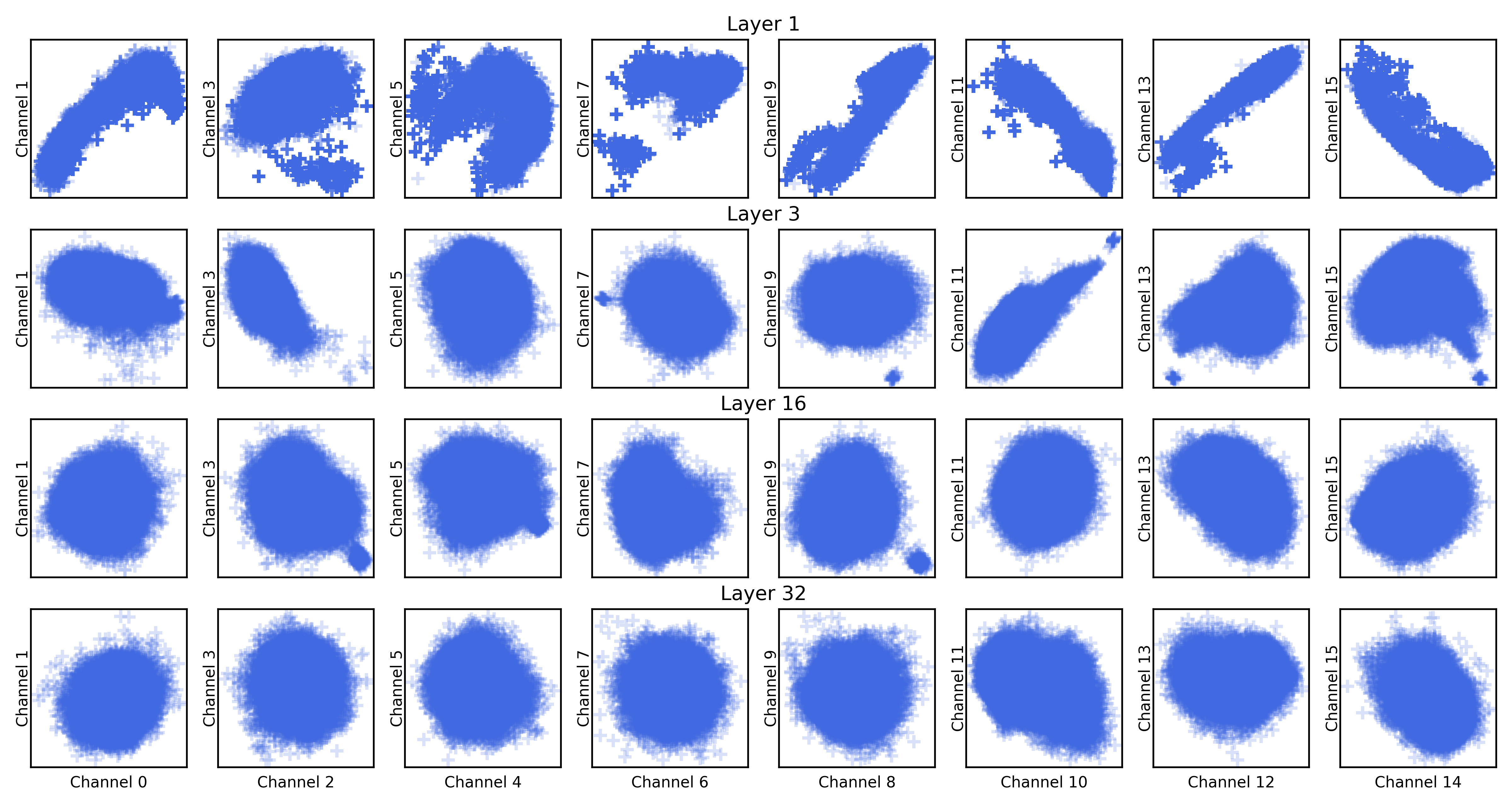</details> Figure 7: 2-dimensional scatter plots of pairs of channels in key activation embeddings of 4 LLaMA-7b layers on WikiText-2. <details> <summary>extracted/5580809/figures/value_emb.png Details</summary>  ### Visual Description ## Scatter Plot Grid: Multi-Layer Channel Analysis ### Overview The image displays a 4x8 grid of scatter plots (32 total), organized by "Layer" (1, 2, 15, 32) and "Channel" (0-15). Each plot contains green circular data points with varying density, and some include isolated "+" symbols. The background is white, with no visible legend or colorbar. ### Components/Axes - **X-axis**: Labeled "Channel" with integer values 0-15 (left to right) - **Y-axis**: Labeled "Layer" with values 1, 2, 15, 32 (top to bottom) - **Data Points**: - Green circles (primary data) - "+" symbols (secondary markers, ~5% of plots) - **Positioning**: - Layer labels appear on the left edge of each column - Channel labels appear at the bottom of each row - No explicit legend visible (color coding inferred) ### Detailed Analysis 1. **Layer 1**: - Channels 0-3: Dense clusters (80-95% coverage) - Channels 7-15: Sparse distributions (30-50% coverage) - Channel 15: Single "+" symbol at (15,1) 2. **Layer 2**: - Channels 0-5: Moderate density (60-80% coverage) - Channels 7-15: Gradual density increase toward center - Channel 13: Distinct "+" symbol at (13,2) 3. **Layer 15**: - Channels 0-7: Uniform circular distributions - Channels 9-15: Concentrated clusters with radial symmetry - Channel 13: "+" symbol at (13,15) 4. **Layer 32**: - Channels 0-15: High uniformity (90-98% coverage) - Channels 4, 12: Subtle density variations - Channel 14: "+" symbol at (14,32) ### Key Observations 1. **Layer Evolution**: - Early layers (1-2) show irregular distributions - Middle layer (15) exhibits transitional symmetry - Final layer (32) demonstrates near-perfect uniformity 2. **Channel Patterns**: - Channels 0, 4, 12 show persistent density variations across layers - Channel 13 consistently contains "+" markers in Layers 1, 2, and 15 - Channel 15 shows increasing density from Layer 1 to 32 3. **Anomalies**: - "+" symbols appear exclusively in Channels 13, 14, and 15 - Layer 1, Channel 0 has a distinct outlier cluster at bottom-left ### Interpretation This visualization appears to track feature distribution evolution across neural network layers. The progression from irregular patterns in early layers to uniform distributions in later layers suggests successful feature abstraction. The "+" markers likely represent critical activation points or anomalies that persist through specific processing stages. Channel 13's consistent marking across multiple layers indicates it may represent a stable feature or error condition. The density variations in Channels 0, 4, and 12 suggest these channels maintain unique characteristics through the network's depth, potentially representing fundamental input features or specialized processing units. </details> Figure 8: 2-dimensional scatter plots of pairs of channels in value activation embeddings of 4 LLaMA-7b layers on WikiText-2.