# Program Synthesis using Inductive Logic Programming for the Abstraction and Reasoning Corpus
**Authors**: Filipe Marinho Rocha, Inês Dutra, Vítor Santos Costa
> INESCTEC-FCUP
## Abstract
The Abstraction and Reasoning Corpus (ARC) is a general artificial intelligence benchmark that is currently unsolvable by any Machine Learning method, including Large Language Models (LLMs). It demands strong generalization and reasoning capabilities which are known to be weaknesses of Neural Network based systems. In this work, we propose a Program Synthesis system that uses Inductive Logic Programming (ILP), a branch of Symbolic AI, to solve ARC. We have manually defined a simple Domain Specific Language (DSL) that corresponds to a small set of object-centric abstractions relevant to ARC. This is the Background Knowledge used by ILP to create Logic Programs that provide reasoning capabilities to our system. The full system is capable of generalize to unseen tasks, since ILP can create Logic Program(s) from few examples, in the case of ARC: pairs of Input-Output grids examples for each task. These Logic Programs are able to generate Objects present in the Output grid and the combination of these can form a complete program that transforms an Input grid into an Output grid. We randomly chose some tasks from ARC that don’t require more than the small number of the Object primitives we implemented and show that given only these, our system can solve tasks that require each, such different reasoning.
123
## 1 Introduction
Machine Learning [5], more specifically, Deep Learning [14], has achieved great successes and surpassed human performance in several fields. These successes, though, are in what is called skill-based or narrow AI, since each DL model is prepared to solve a specific task very well but fails at solving different kind of tasks [18] [13].
It is known Artificial Neural Networks (ANNs) and Deep Learning (DL) suffer from lack of generalization capabilities. Their performance degrade when they are applied to Out-of-Distribution data [12] [8] [27].
Large Language Models (LLMs), more recently, have shown amazing capabilities, shortening the gap between Machine and Human Intelligence. But they still show lack of reasoning capabilities and require lots of data and computation.
The ARC challenge was designed by Francois Chollet in order to evaluate whether our artificial intelligent systems have progressed at emulating human like form of general intelligence. ARC can be seen as a general artificial intelligence benchmark, a program synthesis benchmark, or a psychometric intelligence test [6].
It was presented in 2019 but it still remains an unsolved challenge, and even the best DL models, such as LLMs cannot solve it [15] [4] [3]. GPT-4V, which is GPT4 enhanced for visual tasks [1], is unable to solve it too [26] [19] [23].
It targets both humans and artificially intelligent systems and aims to emulate a human-like form of general fluid intelligence. It is somewhat similar in format to Raven’s Progressive Matrices [22], a classic IQ test format.
It requires, what Chollet describes as, developer-aware generalization, which is a stronger form of generalization, than Out-of-Distribution generalization [6]. In ARC, the Evaluation set, with 400 examples, only features tasks that do not appear in the Training set, with also 400 examples, and all each of these tasks require very different Logical patterns to solve, that the developer cannot foresee. There is also a Test set with 200 examples, which is completely private.
For a researcher setting out to solve ARC, it is perhaps best understood as a program synthesis benchmark [6]. Program synthesis [9] [10] is a subfield of AI with the purpose of generating of programs that satisfy a high-level specification, often provided in the form of example pairs of inputs and outputs for the program, which is exactly the ARC format.
Chollet recommends starting by developing a domain-specific language (DSL) capable of expressing all possible solution programs for any ARC task [6]. Since the exact set of ARC tasks is purposely not formally definable, and can be anything that would only involve Core Knowledge priors, this is challenging.
Objectness is considered one of the Core Knowledge prior of humans, necessary to solve ARC [6]. Object-centric abstractions enable object awareness which seems crucial for humans when solving ARC tasks [2] [11] and is central to general human visual understanding [24]. There is previous work using object-centric approaches to ARC that shows its usefulness [16] [2].
Inductive Logic Programming (ILP) [20] is also considered a Machine Learning method, but to our knowledge it was never applied to the ARC challenge. It can perform Program Synthesis [7] and is known for being able to learn and generalize from few training examples [17] [21].
We developed a Program Synthesis system that uses ILP, on top of Object-centric abstractions, manually defined by us. It does Program synthesis by searching the combination of Logic relations between objects existent in the training examples. This Logic relations are defined by Logic Programs, obtained using ILP.
The full program our system builds, is composed by Logic Programs that are capable of generating objects in the Output Grid.
We selected five random examples that contain only simple geometrical objects and applied our system to these.
Figure 1: Example tasks of the ARC Training dataset with the solutions shown. The goal is to produce the Test Output grid given the Test Input grid and the Train Input-Output grid pairs. We can see the logic behind each task is very different and the relations between objects are key to the solutions.
## 2 Object-centric Abstractions and Representations
Object-centric abstractions reduce substantially the search space by enabling the focus on the relations between objects, instead of individual pixels.
However, there may be multiple ways to interpret the same image in terms of objects, therefore, we keep multiple, overlapping Object representations for the same image.
### 2.1 Objects and Relations between Objects
We have defined manually a simple DSL that is composed by the Objects: Point, Line and Rectangle and the Relations between Objects: LineFromPoint, Translate, Copy, PointStraightPathTo.
Table 1: Object types.
| Point | (x, y, color) |
| --- | --- |
| Line | (x1, y1, x2, y2, color, len, orientation, direction) |
| Rectangle | (x1, y1, x2, y2, x3, y3, x4, y4, color, clean, area) |
Table 2: Relations types.
| LineFromPoint | (point, line, len, orientation, direction) |
| --- | --- |
| Translate | (obj1, obj2, xdir, ydir, color2) |
| Copy | (obj1, obj2, color2, clean) |
| PointStraightPathTo | (point, obj, xdir, ydir, orientation, direction) |
### 2.2 Multiple Representations
An image representation in our object-centric approach is defined by a list of objects (possibly overlapping) and a background color. This representation can build a target image from an empty grid by firstly filling the grid with the background color and then drawing each object on top of it.
An image grid can be defined by multiple Object representations. For example a single Rectangle in an empty grid can also be defined as several Line or Point objects that form the same Rectangle.
Since we don’t know from the start, the Logic behind the transformation of the Input grid into the Output grid, we don’t know if the Object Rectangle is key to this logic (relation between rectangles) or if instead the logic demands using a Line representation for it may involve a relation dependent on lines, such as the LineFromPoint relation.
<details>
<summary>extracted/2405.06399v1/multiple_representations.png Details</summary>
### Visual Description
## Diagram: Input-to-Output Transformation Flow
### Overview
The image displays a technical diagram illustrating a transformation process from a single input state to three distinct output states. The diagram consists of four 10x10 grid matrices, each representing a 2D spatial field. A red highlighted region within each grid represents a "foreground" or "active" area. Red arrows indicate the directional flow of transformation from the "Input" to each of the three "Outputs."
### Components/Axes
* **Grid Structure:** Four separate 10x10 grids. Each grid cell is demarcated by thin white lines on a black background.
* **Labels:**
* **Input:** Located top-left.
* **Output 1:** Located top-right.
* **Output 2:** Located bottom-right.
* **Output 3:** Located bottom-left.
* **Flow Indicators:** Three solid red arrows.
* One arrow points horizontally from the right edge of the "Input" grid to the left edge of the "Output 1" grid.
* One arrow points vertically downward from the bottom edge of the "Input" grid to the top edge of the "Output 3" grid.
* One arrow points diagonally from the bottom-right corner of the "Input" grid to the top-left corner of the "Output 2" grid.
* **Data Representation:** The "data" is the spatial configuration of red-filled cells within each grid. No numerical axes, scales, or legends are present.
### Detailed Analysis
**1. Input Grid (Top-Left):**
* Contains a solid red 2x2 square block.
* **Spatial Position:** The block is centered within the grid. Assuming a 1-indexed grid from the top-left, the red cells occupy rows 5-6 and columns 5-6.
**2. Output 1 Grid (Top-Right):**
* Contains a solid red 2x2 square block, identical in size and shape to the Input.
* **Spatial Position:** The block is also centered, occupying rows 5-6 and columns 5-6.
* **Transformation from Input:** No change in shape, size, or position. The horizontal arrow suggests a direct copy or identity operation.
**3. Output 2 Grid (Bottom-Right):**
* Contains a solid red vertical rectangle of size 1x2 (1 cell wide, 2 cells tall).
* **Spatial Position:** The rectangle is centered horizontally but spans rows 5-6 in column 5.
* **Transformation from Input:** The 2x2 square has been reduced to a 1x2 vertical line. The diagonal arrow suggests a transformation that reduces horizontal dimension while preserving vertical extent in the leftmost column of the original shape.
**4. Output 3 Grid (Bottom-Left):**
* Contains a single red cell.
* **Spatial Position:** The cell is located at row 5, column 5.
* **Transformation from Input:** The 2x2 square has been reduced to its top-left corner cell. The vertical arrow suggests a transformation that reduces the shape to a single point, specifically the origin (top-left) of the original bounding box.
### Key Observations
* **Consistent Origin Point:** All output shapes are anchored to the top-left cell (row 5, column 5) of the original 2x2 input square.
* **Progressive Reduction:** The outputs show a hierarchy of reduction: Output 1 (no reduction) -> Output 2 (50% reduction, vertical axis preserved) -> Output 3 (75% reduction, single point).
* **Directional Semantics:** The arrow directions may symbolically correspond to the type of transformation: horizontal (identity/copy), vertical (column-wise reduction), and diagonal (point-wise reduction).
### Interpretation
This diagram likely illustrates fundamental operations in image processing, matrix manipulation, or cellular automata. The transformations demonstrate:
1. **Identity Operation (Output 1):** The input is passed through unchanged.
2. **Morphological Erosion or Projection (Output 2):** The input is eroded to a vertical line, possibly representing a projection onto the Y-axis or the result of a vertical structuring element.
3. **Downsampling or Feature Extraction (Output 3):** The input is reduced to a single representative point, such as its centroid (approximated here as the top-left corner) or a downsampled pixel.
The diagram serves as a visual specification for how a system should decompose or simplify a 2D input pattern based on different rules or pathways. The clear spatial grounding allows for precise reconstruction of the intended logic without ambiguity.
</details>
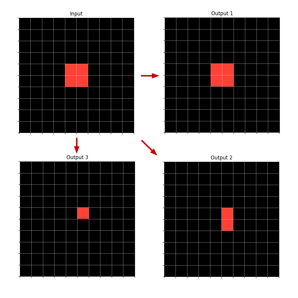
Figure 2: Example of an Input grid with a Rectangle (or with several contiguous Points or Lines) and three possible Output grids, built from the Input, depending on which type of Object representation is used. The Output object can be described by the relation Copy applied to the Input Rectangle or to just one Input Point or Input Line that is part of the same Rectangle.
Likewise, the same image transformation can be explained by different relations.
So we work with multiple and intermingled representations of objects and relations until we get the final program or programs that can transform each of the Training input grids into the output grids and also produce a valid Output grid for the Test Example, which will be the output solution given by our system.
If multiple programs applied separately can produce successfully the same Input-Output Train images transformation, we can use any of this, or select one, for example: the shortest program, which will have more probability of being the correct one, according to the Occam principle.
## 3 ILP
Inductive Logic Programming (ILP) is a form of logic-based Machine Learning. The goal is to induce a hypothesis, a Logic Program or set of Logical Rules, that generalizes given training examples and Background Knowledge (BK). Our DSL composed by Objects and Relations, is the BK given.
As with other forms of ML, the goal is to induce a hypothesis that generalizes training examples. However, whereas most forms of ML use vectors/tensors to represent data, ILP uses logic programs. And whereas most forms of ML learn functions, ILP learns relations.
The fundamental ILP problem is to efficiently search a large hypothesis space. There are ILP approaches that search in either a top-down or bottom-up fashion and others that combine both. We use a top-down approach in our system.
Learning a large program with ILP is very challenging, since the search space can get very big. There are some approaches that try to overcome this.
### 3.1 Divide-and-conquer
Divide-and-conquer approaches [25] divide the examples into subsets and search for a program for each subset. We use a Divide-and-conquer approach but instead of applying it to examples, we apply it to the Objects inside the examples.
## 4 Program Synthesis using ILP
ILP is usually seen as a method for Concept Learning but is capable of building a Logic Program in Prolog, which is Turing-complete, hence, it does Program Synthesis. We extend this by combining Logic Programs to build a bigger program that generates objects in sequence, to fill an empty grid, which corresponds to, procedurally, applying grids transformations to reach the solution.
A Relation can be used to generate objects. All of our Relations, except for PointStraightPathTo, are able to generate Objects given the first Object of the Relation. To generate an unambiguous output, the Relation should be defined by a Logic Program. This Logic Program is built by using ILP in our system.
Example of a logic program in Prolog:
⬇
line_from_point (Point, Line, Len, Orientation, Direction):-
member (Point, Input_points),
equal (Len,5),
equal (Orientation, ’vertical’).
<details>
<summary>extracted/2405.06399v1/line_from_point_example1.png Details</summary>
### Visual Description
## Diagram: Input-Output Grid Transformation
### Overview
The image displays a technical diagram illustrating a transformation process between two 10x10 grids. The left grid is labeled "Input" and contains two isolated colored cells on a black background. The right grid, labeled "Output," shows the result of a transformation where those colored cells have been extended into vertical bars. A red arrow points from the input to the output, indicating the direction of the process.
### Components/Axes
* **Structure:** Two identical 10x10 grids, each composed of 100 square cells defined by thin, light gray grid lines on a black background.
* **Labels:**
* The left grid has the title "Input" centered above it.
* The right grid has the title "Output" centered above it.
* **Visual Elements:**
* **Input Grid:** Contains two single, filled cells.
* One cell is filled with a solid **red** color.
* One cell is filled with a solid **light blue** color.
* **Output Grid:** Contains two vertical bars, each spanning multiple cells.
* One bar is filled with the same **red** color.
* One bar is filled with the same **light blue** color.
* **Arrow:** A solid **red** arrow is positioned between the two grids, pointing from the "Input" grid to the "Output" grid.
### Detailed Analysis
**1. Input Grid (Left) - Component Isolation:**
* **Red Cell:** Located in the **top row (Row 1)**, **column 5** (counting from left to right). It is a single, isolated cell.
* **Blue Cell:** Located in the **bottom row (Row 10)**, **column 6**. It is also a single, isolated cell.
* All other 98 cells in the grid are black (empty).
**2. Output Grid (Right) - Component Isolation:**
* **Red Bar:** A vertical bar occupying **Rows 1 through 5** in **column 5**. It is 5 cells tall.
* **Blue Bar:** A vertical bar occupying **Rows 6 through 10** in **column 6**. It is 5 cells tall.
* The bars are contiguous and directly adjacent where they meet (Row 5, Col 5 and Row 6, Col 6 are diagonally adjacent).
* All other 90 cells in the grid are black (empty).
**3. Transformation Flow:**
The red arrow explicitly defines the relationship: the state on the left ("Input") is processed to produce the state on the right ("Output").
### Key Observations
* **Spatial Relationship:** The output bars originate from the exact column positions of their corresponding input cells. The red bar is in the same column (5) as the red input cell. The blue bar is in the same column (6) as the blue input cell.
* **Vertical Expansion:** The transformation converts a single cell into a vertical bar of length 5.
* **Directional Logic:** The expansion appears to follow a directional rule from the input point:
* The **red** input cell at the **top** expands **downward** to form its bar.
* The **blue** input cell at the **bottom** expands **upward** to form its bar.
* **Non-Overlap:** The two output bars do not overlap in cells. They meet at a diagonal boundary between (Row5, Col5) and (Row6, Col6).
### Interpretation
This diagram visually encodes a specific data transformation or image processing operation. It demonstrates a rule-based mapping where isolated data points (the input cells) are used as seeds to generate extended features (the output bars).
The process suggests a form of **vertical dilation** or **feature propagation** with a fixed kernel size (5 pixels/cells). The direction of propagation (downward from top, upward from bottom) implies the operation is context-aware, possibly using the cell's position within the grid to determine the expansion direction. This could represent operations in computer vision (like morphological dilation with a directional structuring element), data visualization (expanding a point into a timeline or bar), or a simple algorithm for filling space from a starting point.
The clear separation of the two bars in the output indicates the transformation is applied independently to each input seed. The diagram effectively communicates a "before-and-after" state, making the transformation rule intuitive: **"Take each colored point and draw a 5-cell vertical line from it, extending towards the center of the grid."**
</details>
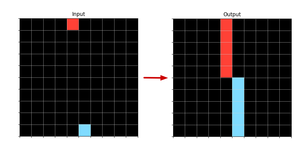
Figure 3: Example of an Input-Output transformation when applied a LineFromPoint Logic Program that is able to generate Lines from Points.
This Logic Program can generate unambiguously, two lines in the Output. The variable Direction is not needed for this, since the points are on the edges of the Grid and so, can only grow into lines in one Direction each.
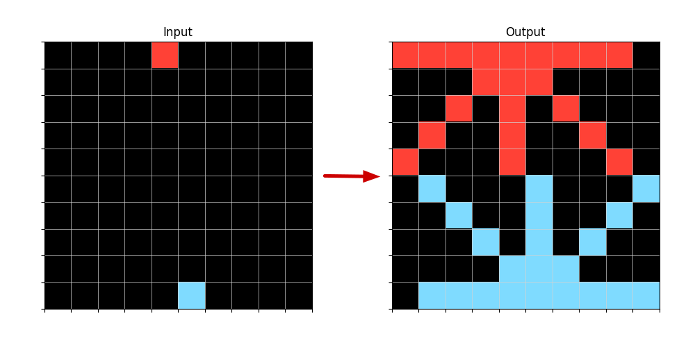
If the program was shorter, it would generate multiple Lines from each Input Point. Example of the same Logic Program without the last term in the body:
⬇
line_from_point (Point, Line, Len, Orientation, Direction):-
member (Point, Input_points),
equal (Len,5).
<details>
<summary>extracted/2405.06399v1/line_from_point_example2.png Details</summary>
### Visual Description
## Diagram: Input-Output Grid Transformation
### Overview
The image displays a technical diagram illustrating a transformation process between two 10x10 grids. The left grid is labeled "Input" and contains two isolated colored cells on a black background. A red arrow points from the Input grid to the right grid, labeled "Output," which shows a complex, symmetrical pattern generated from the initial colored cells. The diagram visually demonstrates an algorithm or process that expands single points into structured patterns.
### Components/Axes
* **Titles:** "Input" (centered above the left grid), "Output" (centered above the right grid).
* **Grids:** Two 10x10 square grids. Each grid is composed of 100 individual cells.
* **Arrow:** A solid red arrow (`→`) positioned between the two grids, indicating the direction of transformation from Input to Output.
* **Color Legend (Implied):**
* **Black:** Background/empty cell.
* **Red:** Active cell (Input: single point; Output: forms an upper pattern).
* **Light Blue/Cyan:** Active cell (Input: single point; Output: forms a lower pattern).
### Detailed Analysis
**Input Grid (Left):**
* **Dimensions:** 10 rows x 10 columns.
* **Content:** 98 black cells, 2 colored cells.
* **Red Cell Position:** Row 1, Column 5 (counting from top-left, 1-based index).
* **Light Blue Cell Position:** Row 10, Column 5.
**Output Grid (Right):**
* **Dimensions:** 10 rows x 10 columns.
* **Content:** A symmetrical pattern of red and light blue cells on a black background. The pattern is vertically mirrored around the central column (Column 5/6).
* **Red Pattern (Upper Half):** Forms a shape resembling a stylized tree, arrow, or fountain. It originates from the top edge and expands downward and outward.
* **Row 1:** Columns 1-8 are red.
* **Row 2:** Columns 4-7 are red.
* **Row 3:** Columns 3, 5, 8 are red.
* **Row 4:** Columns 2, 6, 9 are red.
* **Row 5:** Columns 1, 5, 10 are red.
* **Light Blue Pattern (Lower Half):** Forms a shape resembling a fountain, anchor, or inverted tree. It originates from the bottom edge and expands upward and outward.
* **Row 6:** Columns 2, 5, 10 are light blue.
* **Row 7:** Columns 3, 8 are light blue.
* **Row 8:** Columns 4, 7 are light blue.
* **Row 9:** Columns 5, 6 are light blue.
* **Row 10:** Columns 2-9 are light blue.
* **Black Cells:** Fill all positions not occupied by red or light blue cells.
### Key Observations
1. **Symmetry:** The output pattern exhibits near-perfect vertical symmetry. The left half (Columns 1-5) is a mirror image of the right half (Columns 6-10).
2. **Origin Points:** The red pattern expands downward from the top edge (Row 1), while the light blue pattern expands upward from the bottom edge (Row 10). This corresponds to the vertical positions of the single red and blue cells in the Input grid.
3. **Pattern Logic:** The transformation appears to follow a rule-based expansion, possibly a cellular automaton, a flood-fill algorithm with constraints, or a procedural generation rule. The patterns do not overlap; red and blue cells remain distinct.
4. **Density:** The Input is extremely sparse (2% filled). The Output is significantly denser, with 38 colored cells (38% filled).
### Interpretation
This diagram is a visual proof-of-concept for a generative algorithm. It demonstrates how minimal input—two single pixels—can be transformed into a complex, ordered, and symmetrical output through a deterministic process.
* **What it Suggests:** The process likely simulates concepts like diffusion, growth, or signal propagation from source points. The symmetry implies the application of a consistent rule applied equally in left/right directions. The separation of colors suggests the algorithm treats different "materials" or "signals" independently.
* **Relationships:** The Input defines the seed locations and colors. The Output is the result of applying a transformation function to those seeds over multiple iterations or steps. The arrow is the visual representation of that function.
* **Notable Anomalies:** The patterns are perfectly contained within the grid and do not bleed into each other, indicating a rule that prevents mixing or collision. The output is not a simple geometric expansion (like a circle) but a more intricate, branching structure, hinting at a rule with specific directional biases or conditions.
**In essence, the image documents a computational experiment where simple starting conditions yield complex, aesthetically structured results, highlighting the power of algorithmic generation.**
</details>
Figure 4: Example of an Input-Output transformation when applied a LineFromPoint Logic Program without having the Orientation defined.
So by obtaining Logic Programs through ILP we are indeed constructing a program that generates objects that can fill an empty Test Output grid, in order to reach the solution.
## 5 System Overview
### 5.1 Objects and Relations Retrieval
Our system begins by retrieving all Objects defined in our DSL, in the Input and Output grids for each example of a task. As we reported before, we keep multiple object representations that may overlap in terms of occupying the same pixels in a image.
Then we search for Relations defined in our DSL betweeen the found objects. We search for Relations between Objects only present in the Input Grid: Input-Input Relations, only present in the Output Grid: Output-Output Relations and between Objects in the Input Grid and Output Grid: Input-Output Relations.
The type of Objects previously found can constraint the search for Relations, since some Relations are specific to some kind of Objects.
### 5.2 ILP calls
We then call ILP to create Logic Programs to define only the Relations found in the previous step. This also reduces the space of the search. We start with the Input-Output Relations, since we need to build the Output objects using information from the Input. After we generate some Object(s) in the Output grid we can starting using also Output-Output relations to generate Output Objects from other Output Objects. Input-Input relations can appear in the body of the rules but won’t be the Target Relations to be defined by ILP, since they don’t generate any Object in the Output.
After each ILP call what is considered Input information, increases. The relations and Objects returned by the ILP call that produce an updated Grid, are considered now as it were present in the Input, and this updated Grid is taken as the initial Output grid where to build on, in the subsequent ILP calls.
#### 5.2.1 Candidate Generation
The candidates terms to be added to the Body of the Rule (Horn Clause) are the Objects and Relations found in the Retrieval step (5.1) plus the Equal(X,…), GreaterThan(X,…), LowerThan(X,…), Member(X,…) predicates. GreaterThan and Lowerthan relate only number variables. We also consider aX+b , being X a number variable and a and b, constants in some interval we predefine.
Since we are using Typed Objects and Relations we only need to generate those candidates that are related to each Target Relation variable by type.
For example, in building a Logic Program that defines the Relation: LineFromPoint(point,line,len,orientation,direction) we are going to generate candidates that relate Points or attributes of Points in order to instantiate the first variable Point of the relation. Then we proceed to the other variables (besides the line variable): len, orientation and direction. Len is of type Int, so it is only relevant to be related to other Int variables or constants. The variable Line remains free because it is the Object we want the relation to generate.
#### 5.2.2 Positive and Negative examples
As we have seen in Section 3, FOIL requires positive and negative examples to induce a program. ARC dataset is only composed of Positive examples. So we created a way to represent negative examples.
In our system for each Logic Program the Positive examples are the Objects that this program generates that exist in the Training Data, and the Negative examples are the Objects that the program generates, but don’t exist in the Training Data.
For example, imagine the Ouput in Figure 3 is the correct one, but the program generates all the Lines in Figure 4 like the shorter Prolog program we presented. For this Program the positives it covers would be the two Lines in Figure 3 and the negatives covered would be all the Lines in Figure 4, except for the vertical ones.
Here, our Object-centric approach also reduces the complexity of the search, compared with taking the entire Grid into account, to define what is a positive example or not.
#### 5.2.3 Unification between Training examples
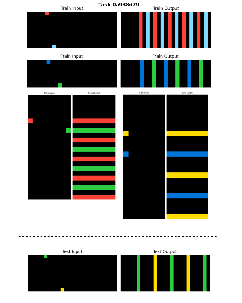
An ILP call is made for each Relation and all of the Task’s Training examples. Our ILP system is constrained to produce Programs that can unify between examples, that is, they are abstract and generalize to two or more of the training examples.
Why two and not all of the training examples? One of the five examples we selected to help us develop our system showed us that a program that solves all Training examples can be too complex and not necessary to solve the Test example.
<details>
<summary>extracted/2405.06399v1/example_unification2.png Details</summary>
### Visual Description
## Diagram: Visual Pattern Transformation Task (Task 0a938d79)
### Overview
The image displays a series of visual examples for a pattern recognition or rule induction task, labeled "Task 0a938d79". It consists of four training examples and one test example, each presented as a pair of grids: a "Train Input" (or "Test Input") and a corresponding "Train Output" (or "Test Output"). The inputs are black grids containing two small, colored squares. The outputs are grids filled with alternating colored bars (either vertical or horizontal) derived from the two colors in the input. The layout is organized with two training examples at the top, two in the middle (side-by-side), and the test example at the bottom, separated by a dashed line.
### Components/Axes
* **Title:** "Task 0a938d79" (top center).
* **Training Examples (4 pairs):**
1. **Top-Left Pair:**
* **Train Input:** A black, landscape-oriented grid. Contains a **red** square near the top-left and a **light blue** square near the bottom-center.
* **Train Output:** A black grid of the same dimensions filled with evenly spaced, alternating **vertical bars** of **red** and **light blue**. The pattern starts with a red bar on the left.
2. **Top-Right Pair:**
* **Train Input:** A black, landscape-oriented grid. Contains a **blue** square near the top-left and a **green** square near the bottom-center.
* **Train Output:** A black grid filled with evenly spaced, alternating **vertical bars** of **blue** and **green**. The pattern starts with a blue bar on the left.
3. **Middle-Left Pair:**
* **Train Input:** A black, portrait-oriented (tall) grid. Contains a **red** square on the left side, approximately midway down, and a **green** square on the right side, also approximately midway down.
* **Train Output:** A black grid filled with evenly spaced, alternating **horizontal bars** of **red** and **green**. The pattern starts with a red bar at the top.
4. **Middle-Right Pair:**
* **Train Input:** A black, portrait-oriented (tall) grid. Contains a **yellow** square near the top-left and a **blue** square near the bottom-left.
* **Train Output:** A black grid filled with evenly spaced, alternating **horizontal bars** of **yellow** and **blue**. The pattern starts with a yellow bar at the top.
* **Test Example (1 pair, below dashed line):**
* **Test Input:** A black, landscape-oriented grid. Contains a **green** square near the top-left and a **yellow** square near the bottom-center.
* **Test Output:** A black grid filled with evenly spaced, alternating **vertical bars** of **green** and **yellow**. The pattern starts with a green bar on the left.
### Detailed Analysis
The core of the task is to infer the transformation rule from the training examples and apply it to the test input. The consistent rule observed across all examples is:
1. **Output Structure:** The output grid is completely filled with alternating bars of the two colors present in the input grid.
2. **Bar Orientation:** The orientation of the bars is determined by the aspect ratio of the input grid.
* If the input grid is **wider than it is tall** (landscape), the output bars are **vertical**.
* If the input grid is **taller than it is wide** (portrait), the output bars are **horizontal**.
3. **Color Order:** The sequence of alternating colors in the output is determined by the relative position of the two colored squares in the input.
* For **vertical bars**, the color of the square positioned **higher** in the input grid becomes the first (leftmost) bar color.
* For **horizontal bars**, the color of the square positioned **more to the left** in the input grid becomes the first (topmost) bar color. (In the fourth example, both squares are on the left, so the higher one—yellow—determines the start).
**Application to Test Example:**
* The Test Input grid is landscape-oriented (wider than tall), so the output must have **vertical bars**.
* The input contains a **green** square (higher) and a **yellow** square (lower). Therefore, the output pattern must start with a **green** bar on the left, followed by alternating yellow and green bars.
* The provided Test Output matches this prediction exactly.
### Key Observations
* The rule is applied consistently across all four training examples without exception.
* The bars in the output are always evenly spaced and cover the entire grid area.
* The number of bars appears to correspond to the resolution of the grid, but the exact pixel count is not discernible from the image.
* The color palette is limited to primary/secondary colors (red, light blue, blue, green, yellow) on a black background, ensuring high contrast.
### Interpretation
This image represents a **visual reasoning or program synthesis task**, likely used to evaluate an AI system's ability to induce a generalizable rule from a small set of examples. The task requires the system to:
1. **Perceive** the visual elements (colored squares on a grid).
2. **Abstract** the relationship between input configuration (grid aspect ratio, square positions) and output pattern (bar orientation, color order).
3. **Generalize** the inferred rule to a novel test case.
The underlying logic is deterministic and based on simple geometric and positional properties. The task tests core cognitive abilities such as pattern recognition, spatial reasoning, and rule-based generalization, which are fundamental to both human and artificial intelligence. The clear, unambiguous examples suggest it is designed for benchmarking or training purposes in a controlled setting.
</details>
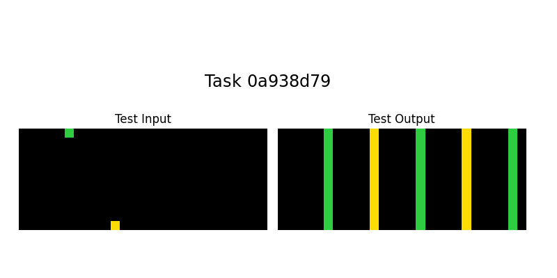
Figure 5: Example task that contains two Train examples with vertical lines and two Train examples with horizontal lines, in the Output grids. The Test example only requires vertical Lines in the same way as the first two Train examples.
In Figure 5 we can see a sample task and derive the logic for its solution: draw Lines from Points until the opposite border of the grid and then Translate these Lines repeatedly in the perpendicular direction of the Lines until the end of the grid.
To unify the four Train examples in this task and following the logic we described for this solution, it would require a more complex program than a solution that only unifies the first two examples.
Let’s see one sequence of Logic programs that solves the first two Train examples, and it would also solve, sucessfully, the Test example:
⬇
line_from_point (Point, Line, Len, Orientation, Direction):-
member (Point, Input_points),
equal (Len, X_dim),
equal (Orientation, ’vertical’).
translate (Line1, Line2, X_dir, Y_dir):-
member (Line1, Input_lines),
equal (X_dir,0),
translate (Input_point1, Input_point2, X_dir, Y_dir),
equal (Y_dir,2* Y_dir).
…
(the same translate program three more times)
The sequence of Logic Programs that would solve the last two Train examples with the Horizontal lines, but wouldn’t solve sucessfully the Test example which has Vertical lines:
⬇
line_from_point (Point, Line, Len, Orientation, Direction):-
member (Point, Input_points),
equal (Len, Y_dim),
equal (Orientation, ’horizontal’).
translate (Line1, Line2, X_dir, Y_dir):-
member (Line1, Input_lines),
equal (Y_dir,0),
translate (Input_point1, Input_point2, X_dir, Y_dir),
equal (X_dir,2* X_dir).
…
(the same translate program three more times)
The Test example only needs two translations in the Output Grid, so a program with more translations would work, since it would fill the entire grid and the extra translations just wouldn’t apply. Our system consider this a valid program.
But if the Test grid was longer and required more translations than present in the Training examples, our program wouldn’t work, since the number of translations wouldn’t produce the exact solution, but an incomplete one. For this kind of tasks we would need to use higher-order constructs as: Do Until, Repeat While or Recursion with a condition, to apply the same Relation a number of times or until some condition fails or is triggered. This is scope of future work.
### 5.3 Rules, Grid states and Search
The first ILP call is made on empty grid states. Each ILP call produces a rule that defines a Relation that generates objects, and returns new Output grid states with these objects added, for each example and the Test example. Each subsequent ILP call is made on the updated Output Grid states.
The search will be on finding the right sequence of Logic Programs that can build the Output Grids, starting from the empty grid. When we have one Program that builds at least one complete Training example Output Grid, consisting of a program that is unified between two or more examples and can also produce a valid solution (not necessarily the correct one) in the Test Output Grid, we consider it the final program.
A valid program is one that builds a consistent theory. For example, a program that generates different colored Lines that intersect with each other, is inconsistent, since both Lines cannot exist in the Output grid (one overlaps the other). We consider programs like this invalid, and discard them, when searching for the complete program.
<details>
<summary>extracted/2405.06399v1/output_state_transition.png Details</summary>
### Visual Description
## Sequential Grid Transformation Diagram
### Overview
The image displays a five-step vertical sequence illustrating a transformation process on a grid-based system. It begins with an "Input Grid" containing two isolated colored cells and progresses through three intermediate states ("Output State 0", "Output State 1", "Output State 2") to a final "Output Grid". Red downward-pointing arrows connect each step, indicating the flow of the process. The visualization demonstrates a pattern of expansion and replication based on initial conditions.
### Components/Axes
* **Grid Structure:** Each step is represented by a rectangular grid of cells. The initial grids ("Input Grid" through "Output State 2") appear to have dimensions of approximately 10 rows by 20 columns. The final "Output Grid" is wider, with an estimated 10 rows by 30 columns.
* **Labels:** Each grid has a centered text label above it:
* "Input Grid"
* "Output State 0"
* "Output State 1"
* "Output State 2"
* "Output Grid"
* **Visual Elements:**
* **Cells:** The background of all grids is black, with a white grid line overlay defining individual cells.
* **Colors:** Two distinct colors are used for data representation: a medium blue and a medium green.
* **Arrows:** Solid red arrows point downward between the grids, connecting the bottom of one grid to the top of the next, establishing the sequence order.
### Detailed Analysis
The transformation process is analyzed step-by-step:
1. **Input Grid:**
* Contains two single, isolated colored cells.
* **Blue Cell:** Located in the top row (Row 1), approximately at Column 8 (counting from the left).
* **Green Cell:** Located in the bottom row (Row 10), approximately at Column 12.
2. **Output State 0:**
* The grid is entirely black. No colored cells are present. This represents a reset or initial blank state following the input.
3. **Output State 1:**
* Two full vertical columns are now colored.
* **Blue Column:** Column 8 is entirely filled with blue from Row 1 to Row 10.
* **Green Column:** Column 12 is entirely filled with green from Row 1 to Row 10.
* **Trend:** The initial single cells from the Input Grid have expanded vertically to fill their entire respective columns.
4. **Output State 2:**
* Four full vertical columns are colored, showing a replication pattern.
* **Blue Column 1:** Column 8 (blue).
* **Green Column 1:** Column 12 (green).
* **Blue Column 2:** Column 16 (blue).
* **Green Column 2:** Column 20 (green).
* **Trend:** The pattern from State 1 (a blue column followed 4 columns later by a green column) has been replicated once to the right. The new blue column is 4 columns right of the first green column, and the new green column is 4 columns right of that.
5. **Output Grid:**
* Six full vertical columns are colored, continuing the replication.
* **Blue Column 1:** Column 8 (blue).
* **Green Column 1:** Column 12 (green).
* **Blue Column 2:** Column 16 (blue).
* **Green Column 2:** Column 20 (green).
* **Blue Column 3:** Column 24 (blue).
* **Green Column 3:** Column 28 (green).
* **Trend:** The replication pattern has been applied a second time, adding another pair of blue and green columns, each spaced 4 columns apart, to the right side of the grid. The grid itself has expanded horizontally to accommodate these new columns.
### Key Observations
* **Pattern Rule:** The core rule appears to be: 1) Expand initial colored cells to fill their columns. 2) Replicate the resulting pattern (a blue column followed by a green column four columns to its right) iteratively to the right.
* **Fixed Spacing:** The horizontal spacing between the start of each colored column in the sequence is consistently 4 columns (e.g., from column 8 to 12, 12 to 16, etc.).
* **Color Order:** The sequence always maintains the order: Blue, Green, Blue, Green...
* **Grid Expansion:** The canvas (grid width) dynamically expands to the right to fit the growing pattern in the final output.
### Interpretation
This diagram visually encodes a deterministic, rule-based process, likely representing an algorithm or a cellular automaton. The process takes sparse input (two points) and generates a structured, periodic output through two clear phases: **vertical expansion** (filling columns) and **horizontal replication** (copying the column pattern with fixed spacing).
The data suggests a system where initial conditions trigger a cascade that fills defined channels (columns) and then propagates that structure in a predictable, repeating manner. This could model concepts in parallel computing (where a task spawns workers in a grid), pattern generation in procedural algorithms, or the behavior of a simple computational system where local rules lead to global order. The clear, step-by-step breakdown makes the underlying logic transparent, emphasizing how simple rules can lead to complex, expanding patterns.
</details>
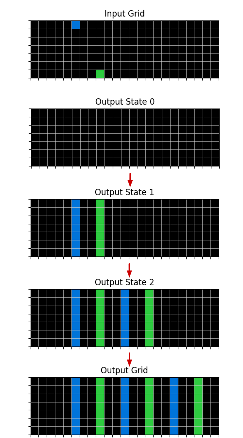
Figure 6: Example of a sucessful sequence of transformations to the Output grid state reaching the final state which is the correct Output grid. These transformations correspond to a sequence of Logic Programs: first transition comes from LineFromPoint Input-Output program, the second and third transitions correspond to the Translate Output-Output programs.
### 5.4 Deductive Search
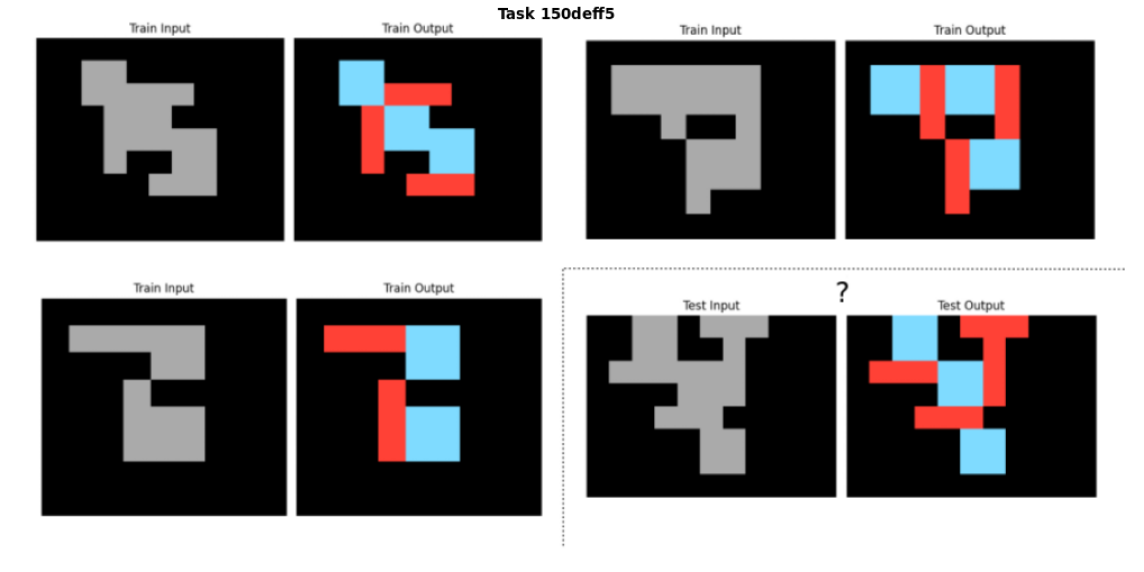
In Figure 7 we can see an example Task that in order to be solved, it would be easier to do it in reverse, that is, the Input Grid being generated from Output information, but since we cannot solve the Test Output Grid by working in this direction, we use a form of Deductive Search to overcome this.
When we apply a Logic Program constructed by ILP, we can have different results depending on the order of the Object Generation. When an Object is generated in the Output Grid, none other Object generated afterwards, can intersect with it.
So the coverage of grid space of the same Logic Program may vary depending on the order of the program application. It is the procedural aspect of our system. When applying several Logic Programs in sequence, this problem gets even bigger.
So when applying the full program to produce the Test Output grid, we use Deductive search to apply the whole program in the way that covers the most surface. Since the final program is one that can cover the whole surface of Train Output grids, we should have a solution that can cover all of the Test Output grid too.
<details>
<summary>extracted/2405.06399v1/last_sample_task.png Details</summary>
### Visual Description
\n
## Visual Reasoning Task Diagram: Task 150deff5
### Overview
The image displays a visual reasoning puzzle, likely from a dataset such as the Abstraction and Reasoning Corpus (ARC). It presents three training examples (input-output pairs) and one test case. The task is to infer the transformation rule from the training examples and apply it to the test input to generate the correct test output. The overall structure is a 2x2 grid of panels, with the test case separated by a dashed line.
### Components/Axes
* **Header Label:** "Task 150deff5" (centered at the top).
* **Panel Structure:** The image is divided into four main quadrants.
* **Top-Left Quadrant:** Contains the first training example.
* **Top-Right Quadrant:** Contains the second training example.
* **Bottom-Left Quadrant:** Contains the third training example.
* **Bottom-Right Quadrant:** Contains the test case, demarcated by a dashed border.
* **Panel Labels:** Each quadrant contains two sub-panels:
* Left sub-panel: Labeled "Train Input" (or "Test Input" for the test case).
* Right sub-panel: Labeled "Train Output" (or "Test Output" for the test case).
* **Grid Content:** Each sub-panel is a square grid (approx. 10x10 cells) with a black background.
* **Input Panels:** Contain a single, contiguous shape (a polyomino) rendered in solid medium gray.
* **Output Panels:** Contain the *exact same shape* as its corresponding input, but its constituent cells are colored either **red** or **light blue**.
* **Test Output Anomaly:** The "Test Output" panel contains a question mark ("?") in its top-right corner, indicating the solution is unknown and must be deduced.
### Detailed Analysis
**Training Example 1 (Top-Left):**
* **Input Shape:** A blocky, irregular shape resembling a stylized "S" or a Tetris piece. It spans approximately 6 cells wide and 7 cells tall.
* **Output Shape:** The same shape is colored. The coloring pattern appears to partition the shape into two distinct, interlocking regions of red and light blue. No two orthogonally adjacent cells within the shape share the same color.
**Training Example 2 (Top-Right):**
* **Input Shape:** A different, more compact shape with a protruding arm. It spans approximately 5 cells wide and 6 cells tall.
* **Output Shape:** Again, the shape is perfectly 2-colored with red and light blue. The pattern is consistent with a "checkerboard" or bipartite coloring applied only to the cells of the shape.
**Training Example 3 (Bottom-Left):**
* **Input Shape:** A third distinct shape, somewhat resembling a blocky "C" or a hook. It spans approximately 6 cells wide and 5 cells tall.
* **Output Shape:** The shape is 2-colored with red and light blue, following the same rule as the previous examples.
**Test Case (Bottom-Right):**
* **Test Input:** A new, more complex shape. It is larger and has a more intricate outline than the training shapes, spanning approximately 7 cells wide and 8 cells tall.
* **Test Output (Partial):** The output panel shows the test input shape partially colored with red and light blue. The coloring is incomplete, and a question mark is present, signifying that the full, correct coloring must be determined by applying the inferred rule.
### Key Observations
1. **Consistent Transformation:** The core task is consistent across all examples: transform a monochromatic gray shape into a two-colored (red and light blue) version of the same shape.
2. **Coloring Rule:** The output coloring is a **proper 2-coloring** (or bipartite coloring) of the shape's grid cells. This means:
* Every cell within the shape is assigned either red or light blue.
* No two cells that share an edge (orthogonal adjacency) have the same color.
* This is equivalent to coloring the shape like a checkerboard, but only using the cells that form the shape.
3. **Spatial Grounding:** The colors are applied directly to the cells of the shape. There is no rotation, scaling, or movement of the shape between input and output.
4. **Test Case Complexity:** The test input shape is more complex, suggesting the rule must be generalized to any connected polyomino.
### Interpretation
The data demonstrates a classic visual logic puzzle centered on **graph coloring**. The shape can be viewed as a graph where each cell is a node, and edges connect orthogonally adjacent cells. The task is to find a valid 2-coloring of this graph.
* **What the data suggests:** The rule is unambiguous and deterministic. For any given connected shape on a grid, there are exactly two valid 2-colorings (which are color inverses of each other). The training examples show one of these two valid colorings for each shape.
* **How elements relate:** The "Input" defines the structure (the graph). The "Output" is a solution to the coloring problem for that structure. The test case presents a new structure for which the solution must be computed.
* **Notable patterns/anomalies:** There are no outliers in the training data; all examples perfectly follow the 2-coloring rule. The only anomaly is the incomplete test output, which is the puzzle's objective. The presence of the question mark explicitly frames the image as a problem to be solved rather than just a display of information.
* **Underlying Principle:** This task tests the ability to recognize and apply an abstract, mathematical rule (bipartite graph coloring) to visual, spatial data. The solution requires understanding adjacency relationships within the shape and propagating a consistent alternating color pattern throughout its entire connected area.
</details>
Figure 7: Example task where the Output Grids are more informative than the Input Grids, to define and apply the Object Relations for the solution.
## 6 Experiments
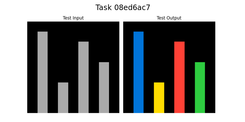
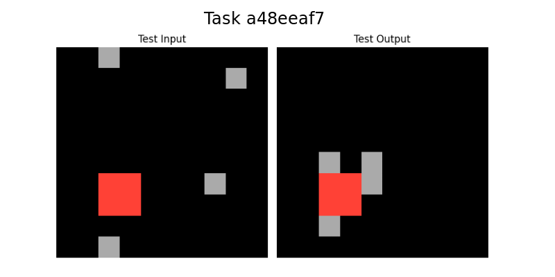
Our system was applied sucessfully to five tasks, the three tasks in Figure 1: 08ed6ac7, a48eeaf7, 7e0986d6, the task in Figure 5: 0a938d79 and the task in Figure 7: 150deff5.
In the Appendices we present the Output solutions in Prolog for each task.
## 7 Conclusion
We showed our system is able to solve the 5 sample tasks selected. When we finish our software implementation we will apply our system to the full Training and Evaluation datasets.
ILP is at the core of our system and we showed that only by providing it with a small DSL or Background Knowledge, ILP is able to construct and represent the Logic behind solutions of ARC tasks.
ILP gives our system abstract learning and generalization capabilities, which is at the core of the ARC challenge.
Since the other ARC tasks may depend on many different DSL primitives, we plan to develop a way to automate the DSL creation.
As we mentioned before, potentially, we are going to need higher-order constructs to solve other tasks and plan to incorporate this into our system.
## References
- Achiam et al. [2023] J. Achiam, S. Adler, S. Agarwal, L. Ahmad, I. Akkaya, F. L. Aleman, D. Almeida, J. Altenschmidt, S. Altman, S. Anadkat, et al. Gpt-4 technical report. arXiv preprint arXiv:2303.08774, 2023.
- Acquaviva et al. [2022] S. Acquaviva, Y. Pu, M. Kryven, T. Sechopoulos, C. Wong, G. Ecanow, M. Nye, M. Tessler, and J. Tenenbaum. Communicating natural programs to humans and machines. Advances in Neural Information Processing Systems, 35:3731–3743, 2022.
- Bober-Irizar and Banerjee [2024] M. Bober-Irizar and S. Banerjee. Neural networks for abstraction and reasoning: Towards broad generalization in machines. arXiv preprint arXiv:2402.03507, 2024.
- Butt et al. [2024] N. Butt, B. Manczak, A. Wiggers, C. Rainone, D. Zhang, M. Defferrard, and T. Cohen. Codeit: Self-improving language models with prioritized hindsight replay. arXiv preprint arXiv:2402.04858, 2024.
- Carbonell et al. [1983] J. G. Carbonell, R. S. Michalski, and T. M. Mitchell. An overview of machine learning. Machine learning, pages 3–23, 1983.
- Chollet [2019] F. Chollet. On the measure of intelligence. arXiv preprint arXiv:1911.01547, 2019.
- Cropper et al. [2022] A. Cropper, S. Dumančić, R. Evans, and S. H. Muggleton. Inductive logic programming at 30. Machine Learning, 111(1):147–172, 2022.
- Farquhar and Gal [2022] S. Farquhar and Y. Gal. What’out-of-distribution’is and is not. In NeurIPS ML Safety Workshop, 2022.
- Gulwani et al. [2015] S. Gulwani, J. Hernández-Orallo, E. Kitzelmann, S. H. Muggleton, U. Schmid, and B. Zorn. Inductive programming meets the real world. Communications of the ACM, 58(11):90–99, 2015.
- Gulwani et al. [2017] S. Gulwani, O. Polozov, R. Singh, et al. Program synthesis. Foundations and Trends® in Programming Languages, 4(1-2):1–119, 2017.
- Johnson et al. [2021] A. Johnson, W. K. Vong, B. M. Lake, and T. M. Gureckis. Fast and flexible: Human program induction in abstract reasoning tasks. arXiv preprint arXiv:2103.05823, 2021.
- Kirchheim et al. [2024] K. Kirchheim, T. Gonschorek, and F. Ortmeier. Out-of-distribution detection with logical reasoning. In Proceedings of the IEEE/CVF Winter Conference on Applications of Computer Vision, pages 2122–2131, 2024.
- Lake et al. [2017] B. M. Lake, T. D. Ullman, J. B. Tenenbaum, and S. J. Gershman. Building machines that learn and think like people. Behavioral and brain sciences, 40:e253, 2017.
- LeCun et al. [2015] Y. LeCun, Y. Bengio, and G. Hinton. Deep learning. nature, 521(7553):436–444, 2015.
- Lee et al. [2024] S. Lee, W. Sim, D. Shin, S. Hwang, W. Seo, J. Park, S. Lee, S. Kim, and S. Kim. Reasoning abilities of large language models: In-depth analysis on the abstraction and reasoning corpus. arXiv preprint arXiv:2403.11793, 2024.
- Lei et al. [2024] C. Lei, N. Lipovetzky, and K. A. Ehinger. Generalized planning for the abstraction and reasoning corpus. arXiv preprint arXiv:2401.07426, 2024.
- Lin et al. [2014] D. Lin, E. Dechter, K. Ellis, J. B. Tenenbaum, and S. H. Muggleton. Bias reformulation for one-shot function induction. 2014.
- Marcus [2018] G. Marcus. Deep learning: A critical appraisal. arXiv preprint arXiv:1801.00631, 2018.
- Mitchell et al. [2023] M. Mitchell, A. B. Palmarini, and A. Moskvichev. Comparing humans, gpt-4, and gpt-4v on abstraction and reasoning tasks. arXiv preprint arXiv:2311.09247, 2023.
- Muggleton and De Raedt [1994] S. Muggleton and L. De Raedt. Inductive logic programming: Theory and methods. The Journal of Logic Programming, 19:629–679, 1994.
- Muggleton et al. [2018] S. Muggleton, W.-Z. Dai, C. Sammut, A. Tamaddoni-Nezhad, J. Wen, and Z.-H. Zhou. Meta-interpretive learning from noisy images. Machine Learning, 107:1097–1118, 2018.
- Raven [2003] J. Raven. Raven progressive matrices. In Handbook of nonverbal assessment, pages 223–237. Springer, 2003.
- Singh et al. [2023] M. Singh, J. Cambronero, S. Gulwani, V. Le, and G. Verbruggen. Assessing gpt4-v on structured reasoning tasks. arXiv preprint arXiv:2312.11524, 2023.
- Spelke and Kinzler [2007] E. S. Spelke and K. D. Kinzler. Core knowledge. Developmental science, 10(1):89–96, 2007.
- Witt et al. [2023] J. Witt, S. Rasing, S. Dumančić, T. Guns, and C.-C. Carbon. A divide-align-conquer strategy for program synthesis. arXiv preprint arXiv:2301.03094, 2023.
- Xu et al. [2023] Y. Xu, W. Li, P. Vaezipoor, S. Sanner, and E. B. Khalil. Llms and the abstraction and reasoning corpus: Successes, failures, and the importance of object-based representations. arXiv preprint arXiv:2305.18354, 2023.
- Ye et al. [2022] N. Ye, K. Li, H. Bai, R. Yu, L. Hong, F. Zhou, Z. Li, and J. Zhu. Ood-bench: Quantifying and understanding two dimensions of out-of-distribution generalization. In Proceedings of the IEEE/CVF Conference on Computer Vision and Pattern Recognition, pages 7947–7958, 2022.
## Appendices
<details>
<summary>extracted/2405.06399v1/08ed6ac7.png Details</summary>
### Visual Description
## Bar Chart Comparison: Task 08ed6ac7
### Overview
The image displays a side-by-side comparison of two bar charts against a solid black background. The overall title, "Task 08ed6ac7," is centered at the top in white text. The left chart is labeled "Test Input" and contains four vertical bars in shades of gray. The right chart is labeled "Test Output" and contains four vertical bars in distinct, solid colors (blue, yellow, red, green). The charts appear to represent a transformation or classification process where an input sequence is mapped to a categorized output.
### Components/Axes
* **Main Title:** "Task 08ed6ac7" (Top center, white text).
* **Subplot Titles:**
* Left Chart: "Test Input" (Centered above the left chart).
* Right Chart: "Test Output" (Centered above the right chart).
* **Axes:** No numerical axes, tick marks, or grid lines are visible. The charts are presented as pure visual comparisons of bar height and color.
* **Legend:** No explicit legend is present. The color coding in the "Test Output" chart serves as an implicit categorical legend.
* **Spatial Layout:** The two charts are positioned horizontally adjacent, with the "Test Input" on the left and the "Test Output" on the right. Each chart occupies approximately half of the image width.
### Detailed Analysis
**Test Input (Left Chart):**
* Contains four vertical bars, all in a uniform medium gray color.
* **Bar 1 (Leftmost):** The tallest bar in the set.
* **Bar 2:** The shortest bar, significantly lower than Bar 1.
* **Bar 3:** The second tallest bar, slightly shorter than Bar 1.
* **Bar 4 (Rightmost):** The third tallest bar, shorter than Bar 3 but taller than Bar 2.
* **Trend/Pattern:** The heights follow a pattern of High, Low, Medium-High, Medium.
**Test Output (Right Chart):**
* Contains four vertical bars, each a different solid color.
* **Bar 1 (Leftmost):** Blue. Its height appears visually identical to the height of the first gray bar in the "Test Input" chart.
* **Bar 2:** Yellow. Its height appears visually identical to the height of the second (shortest) gray bar in the "Test Input" chart.
* **Bar 3:** Red. Its height appears visually identical to the height of the third gray bar in the "Test Input" chart.
* **Bar 4 (Rightmost):** Green. Its height appears visually identical to the height of the fourth gray bar in the "Test Input" chart.
* **Trend/Pattern:** The sequence of heights (High, Low, Medium-High, Medium) is preserved exactly from the input. The only change is the application of distinct colors to each bar.
### Key Observations
1. **Perfect Height Correspondence:** There is a one-to-one mapping in height between each bar in the "Test Input" and its counterpart in the "Test Output." The output does not alter the magnitude (height) of the data.
2. **Categorical Color Assignment:** The transformation from input to output assigns a unique, vibrant color (Blue, Yellow, Red, Green) to each data point, replacing the uniform gray. This strongly suggests a classification or labeling task.
3. **Order Preservation:** The left-to-right order of the bars is maintained between the two charts.
4. **Visual Clarity:** The use of a black background and high-contrast colors (gray for input, primary/secondary colors for output) makes the comparison stark and unambiguous.
### Interpretation
This visualization demonstrates the result of a **classification or labeling algorithm** applied to a sequence of four data points.
* **What the data suggests:** The "Test Input" represents a sequence of raw, unlabeled numerical values (visualized as gray bars of varying height). The "Test Output" represents the same sequence after each value has been assigned to a discrete category. The height (original value) is preserved, but each item is now identified by a color-coded class label (Blue, Yellow, Red, Green).
* **How elements relate:** The direct, side-by-side layout and identical bar heights create an explicit visual link between each input element and its classified output. The color is the only new information added, serving as the category identifier.
* **Notable patterns/anomalies:** The most notable pattern is the perfect preservation of the input sequence's structure. There is no anomaly; the output is a direct, categorized映射 of the input. The choice of four distinct colors implies the model or process has identified four separate classes within this test sample. The specific mapping (e.g., the tallest bar becomes Blue, the shortest becomes Yellow) would be defined by the underlying model's logic, which is not detailed in the chart itself. This chart effectively answers "What were the input values?" and "What category was each one assigned to?" without providing the numerical scale or class names.
</details>
⬇
copy (Line1, Line_out, Color_out, Clean):-
member (Line1, Input_lines),
member (Line2, Input_lines),
member (Line3, Input_lines),
member (Line4, Input_lines),
line_attrs (Line1, X11, Y11, X12, Y12, Color1, Len1,
Orientation1, Direction1),
line_attrs (Line2, X21, Y21, X22, Y22, Color2, Len2,
Orientation2, Direction2),
line_attrs (Line3, X31, Y31, X32, Y32, Color3, Len3,
Orientation3, Direction3),
line_attrs (Line4, X41, Y41, X42, Y42, Color4, Len4,
Orientation4, Direction4),
equal (Color_out, ’blue’),
equal (Clean,100),
greaterthan (Len1, Len2),
greaterthan (Len1, Len3),
greaterthan (Len1, Len4).
copy (Line1, Line_out, Color_out, Clean):-
member (Line1, Input_lines),
member (Line2, Input_lines),
member (Line3, Input_lines),
member (Line4, Input_lines),
line_attrs (Line1, X11, Y11, X12, Y12, Color1, Len1,
Orientation1, Direction1),
line_attrs (Line2, X21, Y21, X22, Y22, Color2, Len2,
Orientation2, Direction2),
line_attrs (Line3, X31, Y31, X32, Y32, Color3, Len3,
Orientation3, Direction3),
line_attrs (Line4, X41, Y41, X42, Y42, Color4, Len4,
Orientation4, Direction4),
equal (Color_out, ’red’),
equal (Clean,100),
lowerthan (Len1, Len2),
greaterthan (Len1, Len3),
greaterthan (Len1, Len4).
copy (Line1, Line_out, Color_out, Clean):-
member (Line1, Input_lines),
member (Line2, Input_lines),
member (Line3, Input_lines),
member (Line4, Input_lines),
line_attrs (Line1, X11, Y11, X12, Y12, Color1, Len1,
Orientation1, Direction1),
line_attrs (Line2, X21, Y21, X22, Y22, Color2, Len2,
Orientation2, Direction2),
line_attrs (Line3, X31, Y31, X32, Y32, Color3, Len3,
Orientation3, Direction3),
line_attrs (Line4, X41, Y41, X42, Y42, Color4, Len4,
Orientation4, Direction4),
equal (Color_out, ’green’),
equal (Clean,100),
lowerthan (Len1, Len2),
lowerthan (Len1, Len3),
greaterthan (Len1, Len4).
copy (Line1, Line_out, Color_out, Clean):-
member (Line1, Input_lines),
member (Line2, Input_lines),
member (Line3, Input_lines),
member (Line4, Input_lines),
line_attrs (Line1, X11, Y11, X12, Y12, Color1, Len1,
Orientation1, Direction1),
line_attrs (Line2, X21, Y21, X22, Y22, Color2, Len2,
Orientation2, Direction2),
line_attrs (Line3, X31, Y31, X32, Y32, Color3, Len3,
Orientation3, Direction3),
line_attrs (Line4, X41, Y41, X42, Y42, Color4, Len4,
Orientation4, Direction4),
equal (Color_out, ’yellow’),
equal (Clean,100),
lowerthan (Len1, Len2),
lowerthan (Len1, Len3),
lowerthan (Len1, Len4).
<details>
<summary>extracted/2405.06399v1/a48eeaf7.png Details</summary>
### Visual Description
\n
## Diagram: Spatial Transformation Task (Task a48eeaf7)
### Overview
The image displays a side-by-side comparison of two square panels, labeled "Test Input" and "Test Output," under the main title "Task a48eeaf7." It illustrates a spatial transformation rule applied to a set of colored squares on a black background. The transformation appears to involve the repositioning of gray squares relative to a central red square.
### Components/Axes
* **Main Title:** "Task a48eeaf7" (centered at the top).
* **Panel Labels:**
* Left Panel: "Test Input" (centered above the left square).
* Right Panel: "Test Output" (centered above the right square).
* **Visual Elements:** Both panels contain a black square field populated with smaller, solid-colored squares.
* **Colors Present:** Black (background), Gray (multiple squares), Red (one square).
* **No numerical axes, legends, or data tables are present.** The information is purely spatial and relational.
### Detailed Analysis
**Test Input Panel (Left):**
* Contains five distinct squares on a black background.
* **Red Square:** Located in the lower-left quadrant. It is the largest colored element.
* **Gray Squares (4 total):**
1. Top-left corner, touching the top edge.
2. Top-right quadrant, not touching any edge.
3. Bottom-left corner, touching the bottom edge.
4. Center-right area, not touching any edge.
* **Spatial Relationship:** The gray squares are scattered with no immediate adjacency to the red square or to each other.
**Test Output Panel (Right):**
* Contains four squares on a black background.
* **Red Square:** Remains in the same lower-left quadrant position as in the input.
* **Gray Squares (3 total):** All are now directly adjacent to the red square, forming a cluster.
1. Positioned directly **above** the red square.
2. Positioned directly **below** the red square.
3. Positioned directly to the **right** of the red square.
* **Spatial Relationship:** The gray squares from the input that were not adjacent to the red square (top-left, top-right, center-right) have been removed or moved. The output shows only gray squares that share a side with the red square.
### Key Observations
1. **Rule-Based Transformation:** The change from input to output follows a clear rule: retain only the gray squares that are orthogonally adjacent (sharing a side, not a corner) to the red square. All non-adjacent gray squares are eliminated.
2. **Positional Constancy:** The red square does not move between the input and output.
3. **Count Change:** The number of gray squares decreases from four in the input to three in the output.
4. **Clustering:** The output creates a compact, cross-shaped cluster centered on the red square.
### Interpretation
This diagram visually defines a computational or logical task, likely from a benchmark or puzzle set (indicated by the ID "a48eeaf7"). The data demonstrates a **spatial filtering operation**.
* **What it suggests:** The underlying rule is: "Given a red square and multiple gray squares, the output should consist of the red square and only those gray squares that are immediate north, south, east, or west neighbors of it."
* **How elements relate:** The red square acts as a **seed or anchor point**. The gray squares are **input elements** evaluated based on their spatial relationship to this anchor. The output is a **filtered subset** of the inputs based on adjacency.
* **Notable patterns/anomalies:** The transformation is deterministic and geometric. There are no outliers; the result is a direct application of the adjacency rule. The task tests an agent's ability to perceive spatial relationships and apply a consistent, location-based filter. The absence of diagonal adjacency in the output is a key detail, specifying the rule's precision.
</details>
⬇
translate (Point1, Point2, X_dir, Y_dir):-
member (Point1, Input_points),
member (Rectangle1, Input_rectangles),
point_straight_path_to (Point1, Rectangle1, X_dir,
Y_dir, Orientation, Direction).
copy (Rectangle1, Rectangle2, Color_out, Clean_out):-
member (Rectangle1, Input_rectangles),
rectangle_attrs (Rectangle1, X1, Y1, X2, Y2, X3, Y3, X4,
Y4, Color, Clean, Area),
equal (Color_out, Color),
equal (Clean_out,100).
<details>
<summary>extracted/2405.06399v1/7e0986d6.png Details</summary>
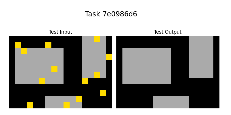
### Visual Description
\n
## Diagram: Task 7e0986d6 - Visual Pattern Transformation
### Overview
The image displays a side-by-side comparison labeled "Test Input" and "Test Output" under the main title "Task 7e0986d6". It illustrates a visual transformation task where a set of yellow squares are removed from a scene containing gray rectangular shapes on a black background. The output shows the same gray shapes in identical positions, but with all yellow squares absent.
### Components/Axes
* **Main Title:** "Task 7e0986d6" (centered at the top).
* **Panel Labels:**
* Left Panel: "Test Input" (centered above the left grid).
* Right Panel: "Test Output" (centered above the right grid).
* **Visual Elements:**
* **Background:** Solid black for both panels.
* **Static Shapes:** Three gray rectangles in fixed positions, identical in both panels.
* **Dynamic Elements:** Multiple small yellow squares present only in the "Test Input" panel.
### Detailed Analysis
**Test Input Panel (Left):**
* **Gray Rectangles:**
1. A large rectangle occupying the left-center area.
2. A tall, narrower rectangle on the right side.
3. A wide, short rectangle at the bottom-center.
* **Yellow Squares (Approximate Count & Placement):**
* **On the large left gray rectangle:** One at the top-left corner, one at the top-right corner, one at the bottom-left corner, and one near the center-right.
* **On the tall right gray rectangle:** One at the top, one at the bottom, and one on the right edge (partially overlapping the black background).
* **On the bottom gray rectangle:** One on the top edge (left side) and one on the right side.
* **On the black background:** One at the bottom-left corner, one near the bottom-right corner, and one on the far right edge (aligned with the tall rectangle's middle).
**Test Output Panel (Right):**
* Contains only the three gray rectangles in the exact same positions and dimensions as in the input panel.
* All yellow squares have been completely removed, leaving only the black background and gray shapes.
### Key Observations
1. **Spatial Consistency:** The gray shapes are perfectly aligned between the input and output, confirming they are the constant, underlying structure.
2. **Element Removal:** The transformation rule is unambiguous: remove all instances of the yellow square element.
3. **Overlap Independence:** Yellow squares were removed regardless of whether they were placed on the gray shapes or the black background.
4. **No Alteration:** The gray shapes themselves are not modified, moved, or resized in the output.
### Interpretation
This diagram represents a classic **visual filtering or object removal task**, common in computer vision, image processing, or abstract reasoning tests. The "data" here is not numerical but **procedural and relational**.
* **What it demonstrates:** The task defines a clear rule: identify and eliminate a specific class of object (yellow squares) from a scene while preserving all other elements (gray rectangles, black background).
* **Relationship between elements:** The gray rectangles act as the "foreground" or "subject" of the scene, while the yellow squares are "noise," "targets," or "artifacts" to be processed. The output is the purified or segmented version of the input.
* **Underlying Logic:** The task tests or demonstrates an agent's ability to perform **selective attention** and **precise manipulation** based on visual attributes (color, shape). The lack of any other changes indicates a single, well-defined operation.
* **Potential Context:** This could be a sample from a dataset for training AI models in image segmentation, a puzzle from an abstract reasoning test (like ARC - Abstraction and Reasoning Corpus), or a specification for a graphics editing macro. The alphanumeric task ID ("7e0986d6") suggests it is one in a series of such problems.
</details>
⬇
copy (Rectangle1, Rectangle2, Color_out, Clean):-
member (Rectangle1, Input_rectangles),
rectangle_attrs (Rectangle1, X1, Y1, X2, Y2, X3, Y3, X4,
Y4, Color, Clean, Area),
equal (Color_out, Color),
equal (Clean,100).
<details>
<summary>extracted/2405.06399v1/0a938d79.png Details</summary>
### Visual Description
## Diagram: Task 0a938d79 - Input/Output Pattern Transformation
### Overview
The image is a technical diagram illustrating a transformation from a "Test Input" to a "Test Output" for a specific task identified as "Task 0a938d79". It visually represents a data processing or pattern generation operation where a sparse input pattern is converted into a dense, repeating output pattern. The diagram consists of a header and two main rectangular panels.
### Components/Axes
* **Header:** Contains the centered title text "Task 0a938d79".
* **Main Panels:** Two black rectangular panels are positioned side-by-side.
* **Left Panel:** Labeled "Test Input" (text centered above the panel).
* **Right Panel:** Labeled "Test Output" (text centered above the panel).
* **Visual Elements:** Colored vertical bars within the black panels.
* **Colors Used:** Green and Yellow.
* **Background:** Solid black for both panels.
### Detailed Analysis
**1. Test Input Panel (Left):**
* **Spatial Grounding:** The panel is a wide, horizontal black rectangle.
* **Content:** Contains two isolated, thin vertical bars.
* **Bar 1 (Green):** Positioned at the far left edge, aligned with the top of the panel. It is a short bar, occupying approximately the top 10-15% of the panel's height.
* **Bar 2 (Yellow):** Positioned roughly at the horizontal center of the panel, aligned with the bottom edge. It is also a short bar, occupying approximately the bottom 10-15% of the panel's height.
* **Trend Verification:** The input is characterized by sparsity and positional asymmetry. The two data points (colored bars) are isolated and located at opposite corners (top-left and bottom-center).
**2. Test Output Panel (Right):**
* **Spatial Grounding:** The panel is a wide, horizontal black rectangle of identical size to the input panel.
* **Content:** Contains a sequence of five, evenly spaced, full-height vertical bars.
* **Bar Sequence (Left to Right):** Green, Yellow, Green, Yellow, Green.
* **Bar Characteristics:** Each bar spans the entire height of the panel (from top edge to bottom edge). They are of uniform width and are separated by consistent black gaps.
* **Trend Verification:** The output demonstrates a clear, repeating pattern. The sequence follows an alternating color pattern (G-Y-G-Y-G) and exhibits high density and regularity compared to the input.
### Key Observations
1. **Pattern Densification:** The core transformation is from a sparse input (2 data points) to a dense output (5 data points).
2. **Pattern Regularization:** The irregular, corner-placed input bars are transformed into a regular, evenly spaced sequence.
3. **Color Sequence Generation:** The output establishes a clear alternating color pattern (Green, Yellow) that is not explicitly present in the input's spatial arrangement. The input's green (top-left) and yellow (bottom-center) may seed this sequence.
4. **Spatial Transformation:** The input's vertical positioning (top vs. bottom) is abstracted away in the output, where all bars are full-height. The output focuses solely on horizontal sequence and color.
### Interpretation
This diagram likely illustrates a fundamental operation in a computational or algorithmic context, such as:
* **Data Augmentation:** Expanding a minimal dataset into a larger, structured one for training or testing.
* **Pattern Completion/Extrapolation:** Inferring and generating a complete, regular pattern from a few sample points.
* **Encoding/Decoding:** The input could represent a compressed or encoded state, and the output represents the decoded, expanded signal.
* **Algorithmic Test Case:** "Task 0a938d79" suggests this is one of many standardized tests for evaluating a system's ability to perform this specific type of spatial and chromatic pattern transformation.
The relationship suggests the system or algorithm under test is designed to recognize latent patterns (like the presence of two colors) and generate a maximally regular, dense output based on that recognition. The notable anomaly is the disconnect between the input's vertical placement and the output's full-height bars, indicating the vertical dimension in the input may be metadata or a secondary feature, while the color and horizontal presence are the primary features driving the transformation.
</details>
⬇
line_from_point (Point, Line, Len, Orientation, Direction):-
member (Point, Input_points),
equal (Len, X_dim),
equal (Orientation, ’vertical’).
translate (Line1, Line2, X_dir, Y_dir):-
member (Line1, Input_lines),
equal (X_dir,0),
translate (Input_point1, Input_point2, X_dir, Y_dir),
equal (Y_dir,2* Y_dir).
translate (Line1, Line2, X_dir, Y_dir):-
member (Line1, Input_lines),
equal (X_dir,0),
translate (Input_point1, Input_point2, X_dir, Y_dir),
equal (Y_dir,2* Y_dir).
translate (Line1, Line2, X_dir, Y_dir):-
member (Line1, Input_lines),
equal (X_dir,0),
translate (Input_point1, Input_point2, X_dir, Y_dir),
equal (Y_dir,2* Y_dir).
translate (Line1, Line2, X_dir, Y_dir):-
member (Line1, Input_lines),
equal (X_dir,0),
translate (Input_point1, Input_point2, X_dir, Y_dir),
equal (Y_dir,2* Y_dir).
<details>
<summary>extracted/2405.06399v1/150deff5.png Details</summary>
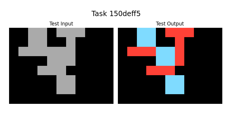
### Visual Description
## Diagram: Task 150deff5 - Input/Output Shape Transformation
### Overview
The image displays a side-by-side comparison of a visual task, labeled "Task 150deff5". It consists of two panels: a "Test Input" on the left and a "Test Output" on the right. Both panels show an identical, complex, connected shape composed of square blocks on a black background. The transformation from input to output involves applying a two-color scheme (red and light blue) to the previously monochromatic gray shape, suggesting a classification, segmentation, or labeling operation.
### Components/Axes
* **Title:** "Task 150deff5" (Centered at the top of the entire image).
* **Panel Labels:**
* "Test Input" (Centered above the left panel).
* "Test Output" (Centered above the right panel).
* **Visual Elements:**
* **Background:** Solid black for both panels.
* **Shape:** A single, contiguous, non-rectilinear shape made of connected square units. The shape's geometry is identical in both panels.
* **Colors:**
* **Test Input:** The entire shape is filled with a uniform medium gray.
* **Test Output:** The shape is segmented into two distinct colors:
* **Red:** Applied to specific contiguous sections of the shape.
* **Light Blue (Cyan):** Applied to other specific contiguous sections of the shape.
* **Spatial Layout:** The two panels are arranged horizontally with a small gap between them. The shape within each panel is positioned slightly left-of-center.
### Detailed Analysis
* **Shape Geometry:** The shape is an irregular, branching structure. It can be described as having a central vertical "spine" with several horizontal and diagonal protrusions. Key features include:
* A top-left horizontal bar.
* A central vertical column.
* A bottom-right horizontal bar.
* A diagonal connection from the top-left to the central column.
* The shape is 8-10 "blocks" in height and 6-8 "blocks" in width at its extremes.
* **Color Mapping (Test Output):** The transformation applies color based on spatial contiguity within the shape.
* **Red Regions:** There are three distinct red regions.
1. A large region covering the top-right portion, including the top of the central spine and a rightward protrusion.
2. A horizontal bar in the middle-left area.
3. A horizontal bar in the lower-middle area.
* **Light Blue Regions:** There are three distinct light blue regions.
1. A region in the top-left, forming the initial horizontal bar and part of the diagonal.
2. A central square block, appearing as a "hub" connecting several arms.
3. A region at the bottom-right, forming the final horizontal bar.
* **Pattern:** The colors do not follow a simple gradient or positional rule (e.g., top=red, bottom=blue). Instead, they appear to segment the shape into its major constituent "limbs" or connected components, with the central hub colored blue.
### Key Observations
1. **Identical Geometry:** The shape's outline and block composition are perfectly preserved from input to output. No pixels are added, removed, or moved.
2. **Discrete Segmentation:** The output uses only two solid colors with no blending or gradients, indicating a hard classification of each part of the shape.
3. **Contiguity Rule:** Regions of the same color are always spatially connected. The color change occurs at points where the shape's connectivity changes (e.g., at junctions).
4. **Central Hub Distinction:** The central connecting block is colored light blue, differentiating it from the red limbs it connects.
### Interpretation
This diagram visually represents a **segmentation or labeling task**, likely from the domain of computer vision, image processing, or procedural generation. The "Test Input" is a raw, unlabeled structure. The "Test Output" demonstrates the result of an algorithm that has analyzed the shape's topology and divided it into meaningful, contiguous sub-regions.
* **What it suggests:** The algorithm successfully identifies and isolates distinct "parts" or "limbs" of a complex object. The two-color scheme might represent a binary classification (e.g., "foreground/background" within the shape, "type A/type B" components) or could be a simplified visualization of a multi-class segmentation where only two classes are shown for clarity.
* **How elements relate:** The input provides the structural data. The output adds a layer of semantic information (the color labels) onto that structure. The relationship is a direct, pixel-perfect mapping where each block's color in the output is determined by an analysis of the input shape's form.
* **Notable patterns/anomalies:** The most notable pattern is the preservation of shape integrity while adding categorical information. There are no anomalies; the transformation is clean and consistent. The choice of red and light blue provides high visual contrast, making the segmentation immediately apparent. The task ID "150deff5" suggests this is one example from a larger dataset or benchmark of similar visual reasoning problems.
</details>
⬇
copy (Rectangle1, Rectangle2, Color_out, Clear):-
member (Rectangle1, Input_rectangles),
rectangle_attrs (X1, Y1, X2, Y2, X3, Y3, X4, Y4, Color,
Rectangle1, Clear, Area),
equiv (Area,4),
equal (Color_out, ’blue’),
equal (Clear,100).
copy (Line1, Line2, Color_out, Clear):-
member (Line1, Input_lines),
line_attrs (Line1, X1, Y1, X2, Y2, Color, Len,
Orientation, Direction),
equiv (Len,3),
equal (Color_out, ’red’),
equal (Clear,100).