# Base of RoPE Bounds Context Length
**Authors**:
- Xin Men (Baichuan Inc.)
- &Mingyu Xu (Baichuan Inc.)
- &Bingning Wang (Baichuan Inc.)
- \ANDQingyu Zhang
- &Hongyu Lin
- &Xianpei Han
- \AND Weipeng Chen
- Baichuan Inc
> Equal contributionCorresponding author,daniel@baichuan-inc.com
Abstract
Position embedding is a core component of current Large Language Models (LLMs). Rotary position embedding (RoPE), a technique that encodes the position information with a rotation matrix, has been the de facto choice for position embedding in many LLMs, such as the Llama series. RoPE has been further utilized to extend long context capability, which is roughly based on adjusting the base parameter of RoPE to mitigate out-of-distribution (OOD) problems in position embedding. However, in this paper, we find that LLMs may obtain a superficial long-context ability based on the OOD theory. We revisit the role of RoPE in LLMs and propose a novel property of long-term decay, we derive that the base of RoPE bounds context length: there is an absolute lower bound for the base value to obtain certain context length capability. Our work reveals the relationship between context length and RoPE base both theoretically and empirically, which may shed light on future long context training.
<details>
<summary>x1.png Details</summary>
### Visual Description
# Technical Document Extraction: RoPE Base Lower Bound Analysis
## 1. Image Overview
This image is a technical line-and-scatter plot on a log-log scale. It illustrates the relationship between the "Context length" of a model and the "Lower bound of RoPE's base." The chart includes a series of discrete data points and a fitted regression line with an associated mathematical formula.
## 2. Component Isolation
### A. Header / Legend Area
* **Location:** Top-left quadrant of the chart area.
* **Legend Item:** A solid red line segment followed by the mathematical expression: $y = 0.0424x^{1.628}$.
* **Visual Confirmation:** The red line in the legend matches the solid red trend line passing through the data points.
### B. Main Chart Area (Data Series)
* **Grid:** Light gray dashed grid lines for both major X and Y axes.
* **Data Points (Scatter):** Represented by dark blue triangles ($\black upward \text{ triangles}$).
* **Trend Line:** A solid red line.
* **Trend Verification:** The data points follow a consistent upward linear path on this log-log scale, indicating a power-law relationship. The red line acts as a "best fit" for these points.
### C. Axis Definitions
* **X-Axis (Horizontal):**
* **Label:** "Context length"
* **Scale:** Logarithmic (Base 10).
* **Markers:** $10^3, 10^4, 10^5, 10^6$.
* **Y-Axis (Vertical):**
* **Label:** "Lower bound of RoPE's base"
* **Scale:** Logarithmic (Base 10).
* **Markers:** $10^4, 10^5, 10^6, 10^7, 10^8$.
## 3. Data Extraction and Reconstructed Table
Based on the log-log scale, the following data points (blue triangles) are estimated from their spatial positioning relative to the grid:
| Context length (x) | Lower bound of RoPE's base (y) | Notes |
| :--- | :--- | :--- |
| $\approx 10^3$ | $\approx 4 \times 10^3$ | First data point |
| $\approx 2 \times 10^3$ | $\approx 1.5 \times 10^4$ | Slightly above the $10^4$ line |
| $\approx 4 \times 10^3$ | $\approx 3 \times 10^4$ | |
| $\approx 8 \times 10^3$ | $\approx 8 \times 10^4$ | Just below the $10^5$ line |
| $\approx 1.5 \times 10^4$ | $\approx 3 \times 10^5$ | |
| $\approx 3 \times 10^4$ | $\approx 6 \times 10^5$ | |
| $\approx 6 \times 10^4$ | $\approx 2 \times 10^6$ | |
| $\approx 1.2 \times 10^5$ | $\approx 8 \times 10^6$ | Just below the $10^7$ line |
| $\approx 2.5 \times 10^5$ | $\approx 4 \times 10^7$ | |
| $\approx 5 \times 10^5$ | $\approx 7 \times 10^7$ | |
| $\approx 10^6$ | $\approx 4 \times 10^8$ | Final data point |
## 4. Key Trends and Mathematical Findings
* **Relationship Type:** The data exhibits a strong power-law relationship, evidenced by the straight-line fit on a log-log plot.
* **Regression Formula:** The relationship is defined by the equation:
$$y = 0.0424x^{1.628}$$
* **Growth Rate:** The exponent of $1.628$ indicates that the lower bound of the RoPE (Rotary Positional Embedding) base grows super-linearly with respect to the context length. Specifically, as the context length increases by a factor of 10, the lower bound increases by a factor of approximately $10^{1.628} \approx 42.46$.
* **Observation:** The blue triangle data points show minor variance (noise) around the red regression line but maintain a very high correlation with the predicted model.
</details>
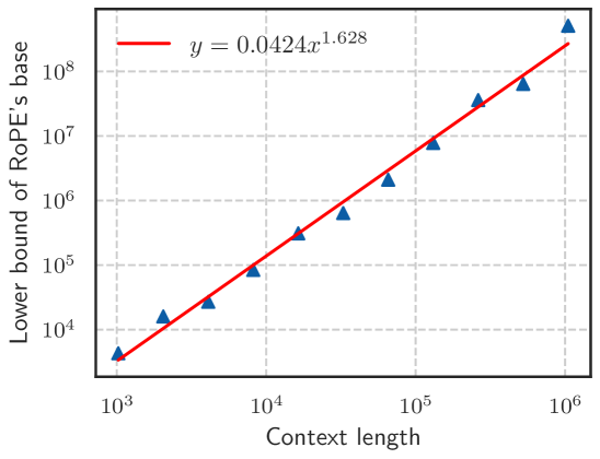
Figure 1: Context length and its corresponding lower bound of RoPE’s base value.
1 Introduction
In the past few years, large language models have demonstrated surprising capabilities and undergone rapid development. By now, LLMs have been widely applied across various domains, including chatbots, intelligent agents, and code assistants (Achiam et al., 2023; Jiang et al., 2023b). The Transformer (Vaswani et al., 2017), based on the attention mechanism, has been the most popular backbone of LLMs due to its good performance and scaling properties (Tay et al., 2022). One of the key component modules in the Transformer is position embedding, which is introduced to embed positional information that is vital for processing sequential data. Rotary position embedding (RoPE), which encodes relative distance information in the form of absolute position embedding (Su et al., 2024), has been a popular choice and applied in many LLMs (Touvron et al., 2023a; Yang et al., 2023; Bai et al., 2023).
RoPE introduces no training parameters and shows improvement in language modeling and many other tasks (Su et al., 2024; Heo et al., 2024). One reason that RoPE is widely used is its ability for context length extrapolation (Peng et al., 2023b; Chen et al., 2023), which extends the context length of a trained LLM without expensive retraining. In practice, many works (Touvron et al., 2023a; Liu et al., 2024a; Young et al., 2024) have successfully extended the window length by simply increasing base value, the only one hyper-parameter in RoPE, and fine-tuning on long texts.
The reasons behind the success of these long context extensions are often explained as avoiding out-of-distribution (OOD) rotation angles (Liu et al., 2024b; Han et al., 2023) in RoPE, meaning the extended context length (OOD) can be mapped to the in-distribution context length that has been properly trained. Based on the OOD theory, a recent study (Liu et al., 2024b) finds that a smaller base can mitigate OOD and is beneficial for the model’s ability to process long contexts, which inspires us to further study the relationship between the base of RoPE and the length of context the model can process.
In this paper, we find that the model may show superficial long context capability with an inappropriate RoPE base value, in which case the model can only preserve low perplexity but loses the ability to retrieve long context information. We also show that the out-of-distribution (OOD) theory in position embedding, which motivates most length extrapolation works (Peng et al., 2023b; Chen et al., 2023; Liu et al., 2024b), is insufficient to fully reflect the model’s ability to process long contexts. Therefore, we revisit the role of RoPE in LLMs and derive a novel property of long-term decay in RoPE: the ability to attend more attention to similar tokens than random tokens decays as the relative distance increases. While previous long context works often focus on the relative scale of the RoPE base, based on our theory, we derive an absolute lower bound for the base value of RoPE to obtain a certain context length ability, as shown in Figure 1. To verify our theory, we conducted thorough experiments on various LLMs such as Llama2-7B (Touvron et al., 2023b), Baichuan2-7B (Yang et al., 2023) and a 2-billion model we trained from scratch, demonstrating that this lower bound holds not only in the fine-tuning stage but also in the pre-training stage.
We summarize the contributions of the paper as follows:
- Theoretical perspective: we derive a novel property of long-term decay in RoPE, indicating the model’s ability to attend more to similar tokens than random tokens, which is a new perspective to study the long context capability of the LLMs.
- Lower Bound of RoPE’s Base: to achieve the expected context length capability, we derive an absolute lower bound for RoPE’s base according to our theory. In short, the base of RoPE bounds context length.
- Superficial Capability: we reveal that if the RoPE’s base is smaller than a lower bound, the model may obtain superficial long context capability, which can preserve low perplexity but lose the ability to retrieve information from long context.
2 Background
In this section, we first introduce the Transformer and RoPE, which are most commonly used in current LLMs. Then we discuss long context methods based on the OOD of rotation angle theory.
2.1 Attention and RoPE
The LLMs in current are primarily based on the Transformer (Vaswani et al., 2017). The core component of it is the calculation of the attention mechanism. The naive attention can be written as:
$$
\displaystyle A_{ij} \displaystyle=q_{i}^{T}k_{j} \displaystyle\text{ATTN}(X) \displaystyle=\text{softmax}(A/\sqrt{d})\ v, \tag{1}
$$
where $A∈ R^{L× L}$ $q,k,v∈ R^{d}$ . Position embedding is introduced to make use of the order of the sequence in attention.
RoPE (Su et al., 2024) implements relative position embedding through absolute position embedding, which applies rotation matrix into the calculation of the attention score in Eq. 1, which can be written as:
$$
\displaystyle A_{ij}=(R_{i,\theta}q_{i})^{T}(R_{j,\theta}k_{i})=q_{i}^{T}R_{j-i,\theta}k_{j}=q_{i}^{T}R_{m,\theta}k_{j}, \tag{3}
$$
where $m=j-i$ is the relative distance of $i$ and $j$ , $R_{m,\theta}$ is a rotation matrix denoted as:
$$
\displaystyle\left[\begin{array}[]{ccccccc}cos(m\theta_{0})&-sin(m\theta_{0})&0&0&\cdots&0&0\\
sin(m\theta_{0})&cos(m\theta_{0})&0&0&\cdots&0&0\\
0&0&cos(m\theta_{1})&-sin(m\theta_{1})&\cdots&0&0\\
0&0&sin(m\theta_{1})&cos(m\theta_{1})&\cdots&0&0\\
\vdots&\vdots&\vdots&\vdots&\ddots&\vdots&\vdots\\
0&0&0&0&\cdots&cos(m\theta_{d/2-1})&-sin(m\theta_{d/2-1})\\
0&0&0&0&\cdots&sin(m\theta_{d/2-1})&cos(m\theta_{d/2-1})\end{array}\right] \tag{11}
$$
Generally, the selection of rotation angles satisfies $\theta_{i}=base^{-2i/d}$ , the typical base value for current LLMs is 10,000, and the base of RoPE in LLMs is shown in Table 1.
Table 1: The setting of RoPE’s base and context length in various LLMs.
| Base | 10,000 | 10,000 | 500,000 | 1,000,000 | 10,000 |
| --- | --- | --- | --- | --- | --- |
| Length | 2,048 | 4,096 | 8,192 | 32,768 | 4,096 |
<details>
<summary>x2.png Details</summary>
### Visual Description
# Technical Document Extraction: RoPE vs. Context-size Analysis
## 1. Image Overview
This image is a line graph illustrating the relationship between "RoPE" (Rotary Positional Embedding) values and "Context-size" in a machine learning context. The graph highlights the behavior of the embedding as the context window extends beyond its original training limits.
## 2. Component Isolation
### A. Header/Title
* No explicit title is present at the top of the image.
### B. Main Chart Area
* **Type:** 2D Line Plot with shaded background regions.
* **X-Axis (Horizontal):**
* **Label:** "Context-size"
* **Major Tick Markers:** 0, 10000, 20000, 30000.
* **Minor Tick Markers:** Increments of 2000 (e.g., 2000, 4000, 6000, 8000).
* **Y-Axis (Vertical):**
* **Label:** "RoPE"
* **Major Tick Markers:** -1.0, -0.5, 0.0, 0.5, 1.0.
* **Minor Tick Markers:** Increments of 0.1.
* **Gridlines:** Horizontal grey lines are present at y-values: -1.0, -0.5, 0.0, 0.5, 1.0.
### C. Shaded Regions (Background)
* **Light Blue Region:** Extends from x = 0 to approximately x = 4000. This represents the "standard" or "original" context window.
* **Light Red/Pink Region:** Extends from approximately x = 4000 to the end of the x-axis (approx. 33000).
* **Embedded Text:** "Extended context" is centered within this region at roughly [x=23000, y=0.05].
## 3. Data Series Analysis
### Trend Verification
* **Series:** Single dark blue solid line.
* **Visual Trend:** The line follows a sinusoidal (specifically, a cosine-like) curve. It starts at its maximum value at x=0, slopes downward through the x-axis, reaches a minimum, and begins to slope upward again at the far right of the chart.
### Data Point Extraction (Estimated)
| Context-size (x) | RoPE Value (y) | Region |
| :--- | :--- | :--- |
| 0 | 1.0 | Standard (Blue) |
| 4000 | ~0.9 | Boundary |
| 10000 | ~0.5 | Extended (Red) |
| 14000 | 0.0 | Extended (Red) |
| 20000 | ~-0.6 | Extended (Red) |
| 27000 | -1.0 (Local Minimum) | Extended (Red) |
| 33000 | ~-0.8 | Extended (Red) |
## 4. Technical Summary
The chart visualizes how a specific dimension of a Rotary Positional Embedding (RoPE) oscillates as the sequence length (Context-size) increases.
1. **Standard Context:** Within the first 4,000 tokens (blue area), the RoPE value remains high (between 1.0 and 0.9), indicating high correlation or specific positional encoding for short-range dependencies.
2. **Extended Context:** As the context size enters the "Extended context" zone (red area), the value crosses zero at approximately 14,000 tokens and reaches a full phase inversion (-1.0) at approximately 27,000 tokens.
This visualization is typically used to demonstrate the "out-of-distribution" behavior of positional embeddings when a model is pushed beyond the sequence length it was originally trained on, showing the periodic nature of the encoding mechanism.
</details>
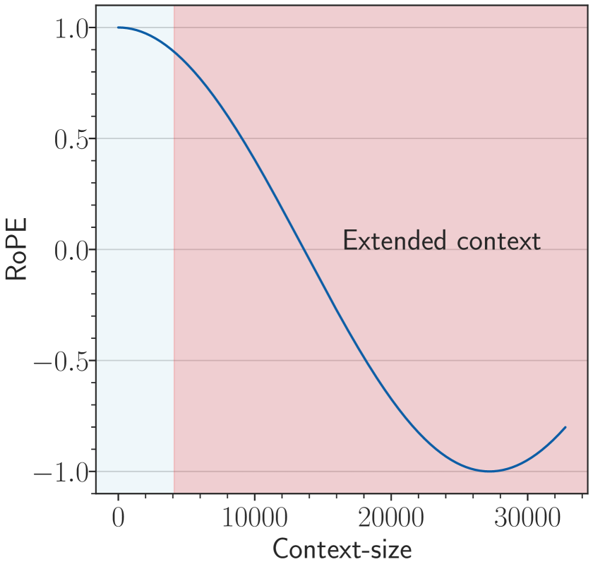
(a) base=1e4
<details>
<summary>x3.png Details</summary>
### Visual Description
# Technical Document Extraction: Context-Size Periodic Waveform Analysis
## 1. Component Isolation
The image is a technical line chart plotted on a Cartesian coordinate system. It is segmented into two distinct background regions to differentiate operational phases.
* **Header:** None present.
* **Main Chart Area:** Contains a single continuous blue oscillating line, two colored background regions, and one text annotation.
* **Footer:** Contains the X-axis label and numerical scale.
## 2. Axis and Label Extraction
### X-Axis (Horizontal)
* **Label:** `Context-size`
* **Scale Range:** 0 to approximately 33,000.
* **Major Tick Markers:** `0`, `10000`, `20000`, `30000`.
* **Minor Tick Markers:** Present at intervals of 1,000 units.
### Y-Axis (Vertical)
* **Label:** None explicitly stated (represents amplitude).
* **Scale Range:** -1.0 to 1.0.
* **Major Tick Markers:** `-1.0`, `-0.5`, `0.0`, `0.5`, `1.0`.
* **Minor Tick Markers:** Present at intervals of 0.1 units.
* **Gridlines:** Horizontal grey lines are present at every major Y-axis tick marker.
## 3. Data Series Analysis
### Series 1: Blue Oscillating Line
* **Color:** Dark Blue.
* **Trend Verification:** The line follows a consistent, undamped sinusoidal (cosine-like) pattern. It begins at a peak of 1.0 at $x=0$, descends to a trough of -1.0, and repeats this cycle with a constant frequency and amplitude across the entire X-axis range.
* **Key Data Points:**
* **Start Point:** [0, 1.0]
* **Amplitude:** 1.0 (Peak-to-peak amplitude of 2.0).
* **Periodicity:** There are approximately 11 full cycles shown between 0 and 33,000. This suggests a period of roughly 3,000 units per cycle.
## 4. Regional Segmentation and Annotations
The chart area is divided into two vertical background zones:
| Region | X-Axis Range (Approx) | Background Color | Description |
| :--- | :--- | :--- | :--- |
| **Training/Base Context** | 0 to 4,000 | Light Blue | Represents the initial context window. |
| **Extended Context** | 4,000 to 33,000+ | Light Red/Pink | Represents the expansion of the context window. |
### Embedded Text
* **Content:** `Extended context`
* **Spatial Grounding:** Located centrally within the red background region, approximately at coordinates [16000, 0.05].
* **Significance:** This label identifies the red-shaded area as the "Extended context" zone, indicating that the periodic signal (likely representing positional embeddings or attention patterns) maintains stability even when the context size exceeds the initial training window.
## 5. Summary of Technical Information
This chart visualizes the stability of a periodic function (likely a Rotary Positional Embedding or similar mechanism in a Transformer model) as the **Context-size** increases. The data demonstrates that the signal's frequency and amplitude remain perfectly consistent when transitioning from the base context (0 - 4,000, blue zone) into the **Extended context** (4,000 - 33,000, red zone), suggesting successful extrapolation or scaling of the underlying mechanism.
</details>
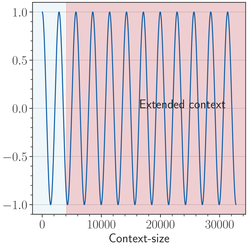
(b) base=500
<details>
<summary>x4.png Details</summary>
### Visual Description
# Technical Document Extraction: Context-size Performance Chart
## 1. Component Isolation
* **Header:** None present.
* **Main Chart Area:** A line graph plotting a performance metric (Y-axis) against "Context-size" (X-axis). The background is divided into two distinct colored regions.
* **Footer:** Contains the X-axis label and major tick marks.
## 2. Axis and Labels
* **X-axis Title:** `Context-size`
* **X-axis Scale:** Linear, ranging from 0 to approximately 33,000.
* **Major Ticks:** 0, 10000, 20000, 30000.
* **Minor Ticks:** Present at intervals of 1,000 and 5,000.
* **Y-axis Title:** None explicitly labeled, but represents a normalized value or probability.
* **Y-axis Scale:** Linear, ranging from 0.88 to 1.00.
* **Major Ticks:** 0.90, 0.92, 0.94, 0.96, 0.98, 1.00.
* **Gridlines:** Horizontal grey lines correspond to each major Y-axis tick.
* **Embedded Text:** "Extended context" is located in the center-right of the plot area.
## 3. Background Regions (Spatial Grounding)
The chart area is divided vertically into two shaded regions:
1. **Light Blue Region (Left):** Extends from X = 0 to approximately X = 4,000. This represents the standard or baseline context window.
2. **Light Red Region (Right):** Extends from approximately X = 4,000 to the end of the X-axis (approx. 33,000). This region is associated with the "Extended context" label.
## 4. Data Series Analysis
### Series 1: Standard Performance (Solid Blue Line)
* **Visual Trend:** The line starts at (0, 1.00) and exhibits a very sharp, steep downward slope.
* **Key Data Points:**
* **Start:** [0, 1.00]
* **End:** Terminates abruptly at approximately [4000, 0.89].
* **Observation:** This series represents a rapid degradation in performance as the context size increases beyond a very small threshold, failing completely shortly after the 4,000 mark.
### Series 2: Extended Performance (Dash-Dot Red Line)
* **Visual Trend:** The line starts at (0, 1.00) and exhibits a much more gradual, concave downward slope.
* **Key Data Points:**
* **Start:** [0, 1.00]
* **Mid-point (approx):** [16000, 0.97]
* **End:** [32768 (approx), 0.89]
* **Observation:** This series maintains significantly higher performance over a much larger context window compared to the blue series. It reaches the same degradation level (0.89) at ~32k that the blue series reached at ~4k.
## 5. Summary of Findings
The chart illustrates the effectiveness of an "Extended context" method (Red Dash-Dot line) compared to a baseline method (Blue Solid line).
* **Baseline:** Performance drops precipitously, losing ~11% of its value within the first 4,000 units of context size.
* **Extended:** Performance is preserved much longer, maintaining >95% of its value up to approximately 22,000 units and only reaching the 11% degradation point at roughly 32,000 units.
* **Conclusion:** The extended context method provides approximately an 8x increase in usable context size for the same level of performance degradation.
</details>
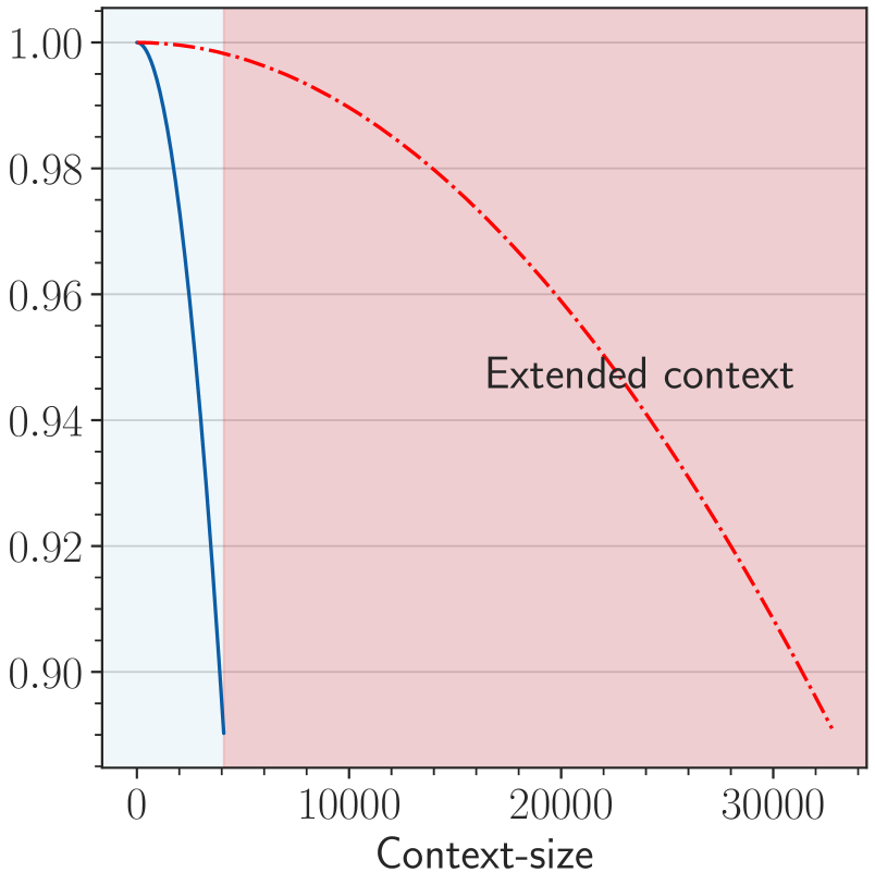
(c) base= $b· s^{\frac{d}{d-2}}$
Figure 2: An illustration of OOD in RoPE when we extend context length from 4k to 32k, and two solutions to avoid the OOD. We show the last dimension as it is the lowest frequency part of RoPE, which suffers OOD mostly in extrapolation. (a) For a 4k context-length model with base value as 1e4, when we extend the context length to 32k without changing the base value, the context length from 4k to 32k is OOD for RoPE (red area in the figure). (b) OOD can be avoided with a small base value like 500 (Liu et al., 2024b), since the full period has been fitted during fine-tuning stage. (c) We set base as $b· s^{\frac{d}{d-2}}$ from NTK (Peng et al., 2023b).The blue line denotes the pre-training stage (base=1e4) and the red dashed line denotes the fine-tuning stage (base= $b· s^{\frac{d}{d-2}}$ ), we can observe that the RoPE’s rotation angle of extended positions is in-distribution.
2.2 OOD theory of relative rotation angle
Based on RoPE, researchers have proposed various methods to extend the long context ability of LLMs, among which representatives are PI (Chen et al., 2023) and NTK-series (NTK-aware (bloc97, 2023), YaRN (Peng et al., 2023b), and Dynamical-NTK (emozilla, 2023)). Those methods depend on the relative scale $s=T_{\text{new}}/T_{\text{origin}}$ , where $T_{\text{origin}}$ is the training length of the original pre-trained model and $T_{\text{new}}$ is the training length in long-context fine-tuning.
PI
PI directly interpolates the position embedding, and the calculation of $A_{ij}$ becomes:
$$
\displaystyle A_{ij}=(R_{i/s}q_{i})^{T}(R_{j/s}k_{i})=q_{i}^{T}R_{(j-i)/s}k_{j}=q_{i}^{T}R_{m/s}k_{j}, \tag{12}
$$
In other words, the position embedding of the token at position $i$ in pre-training becomes $i/s$ in fine-tuning, ensuring the position embedding range of the longer context remains the same as before.
NTK-series
The idea is that neural networks are difficult to learn high-frequency features, and direct interpolation can affect the high-frequency parts. Therefore, the NTK-aware method achieves high-frequency extrapolation and low-frequency interpolation by modifying the base value of RoPE. Specifically, it modifies the base $b$ of the RoPE to:
$$
\displaystyle b_{\text{new}}=b\ s^{\frac{d}{d-2}}. \tag{13}
$$
The derivation of this expression is derived from $T_{\text{new}}b_{\text{new}}^{-\frac{d-2}{d}}=T_{\text{origin}}b^{-\frac{d-2}{d}}$ to ensure that the lowest frequency part being interpolated.
A recent study (Liu et al., 2024b) proposes to set a much smaller base (e.g. 500), in which case $\theta_{i}=base^{-\frac{2i}{d}}$ is small enough and typical training length (say 4,096) fully covers the period of $\cos(t-s)\theta_{i}$ , so the model can obtain longer context capabilities.
One perspective to explain current extrapolation methods is the OOD of rotation angle (Liu et al., 2024b; Han et al., 2023). If all possible values of $\cos(t-s)\theta_{i}$ have been fitted during the pre-training stage, OOD would be avoided when processing longer context. Figure 2 demonstrates how these methods avoid OOD of RoPE.
3 Motivation
<details>
<summary>x5.png Details</summary>
### Visual Description
# Technical Document Extraction: Perplexity vs. Context Size Chart
## 1. Component Isolation
* **Header/Legend Region:** Located in the top-right quadrant of the plot area.
* **Main Chart Area:** A line graph with a grid background, plotting Perplexity against Context Size.
* **Axes:** Y-axis (left) representing Perplexity; X-axis (bottom) representing Context size.
---
## 2. Metadata and Labels
* **Y-Axis Title:** Perplexity
* **X-Axis Title:** Context size
* **Y-Axis Markers:** 20, 40, 60, 80, 100
* **X-Axis Markers:** 0, 25000, 50000, 75000, 100000, 125000
* **Legend (Spatial Placement: Top-Right [x≈0.6, y≈0.8]):**
* **Blue Line:** `finetune on 32k(base=500)`
* **Red Line:** `Llama2-7B-Baseline`
---
## 3. Data Series Analysis and Trend Verification
### Series 1: Llama2-7B-Baseline (Red Line)
* **Trend Description:** The line starts at a low perplexity (below 10) at a context size of 0. It remains stable for a very short duration and then exhibits a near-vertical upward spike, exiting the top of the chart (Perplexity > 100) before reaching a context size of approximately 4,000.
* **Key Data Points:**
* Context 0: Perplexity ≈ 8
* Context ~2,500: Perplexity begins sharp ascent.
* Context ~4,000: Perplexity > 100 (Off-chart).
### Series 2: finetune on 32k(base=500) (Blue Line)
* **Trend Description:** This line starts at a similar low perplexity (below 10) and maintains a very gradual, slightly oscillating upward slope across the entire horizontal range of the chart. It demonstrates extreme stability compared to the baseline.
* **Key Data Points:**
* Context 0: Perplexity ≈ 8
* Context 32,000: Perplexity ≈ 8-9
* Context 62,500: Perplexity ≈ 9
* Context 100,000: Perplexity ≈ 10
* Context 125,000: Perplexity ≈ 11
---
## 4. Comparative Summary
The chart illustrates the performance of two Large Language Models (LLMs) in terms of perplexity (where lower is better) as the input context window increases.
1. **Llama2-7B-Baseline:** This model fails rapidly as the context size exceeds its training window. Its perplexity explodes (goes to infinity/off-chart) almost immediately after the 2,000-4,000 token mark.
2. **finetune on 32k(base=500):** This model shows significant architectural or fine-tuning improvements. Despite being "finetuned on 32k," it maintains a low and stable perplexity (under 12) even when the context size is extended to 125,000 tokens, which is nearly 4x its stated fine-tuning length.
---
## 5. Grid and Scale Details
* **Grid:** Light gray dashed lines.
* **X-axis Major Ticks:** Every 25,000 units.
* **Y-axis Major Ticks:** Every 20 units.
* **Language:** English (No other languages detected).
</details>
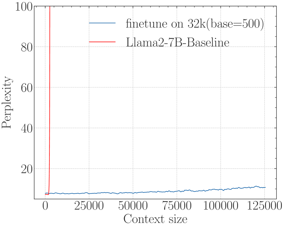
(a) Perplexity
<details>
<summary>x6.png Details</summary>
### Visual Description
# Technical Data Extraction: Model Accuracy vs. Context Length
## 1. Component Isolation
* **Header:** None present.
* **Main Chart Area:** A 2D line graph plotted on a Cartesian coordinate system with a light-gray dashed grid.
* **Legend:** Located in the center-right of the plot area.
* **Axes:** Y-axis (left) representing "Accuracy" and X-axis (bottom) representing "Context length".
---
## 2. Axis Labels and Markers
### Y-Axis (Vertical)
* **Label:** Accuracy
* **Scale:** Linear, ranging from 0.0 to 1.0.
* **Major Tick Markers:** 0.0, 0.2, 0.4, 0.6, 0.8, 1.0.
### X-Axis (Horizontal)
* **Label:** Context length
* **Scale:** Linear, ranging from approximately 500 to 5500.
* **Major Tick Markers:** 1000, 2000, 3000, 4000, 5000.
---
## 3. Legend and Data Series Identification
The legend contains two entries, which correspond to the two lines plotted:
1. **Blue Line (Dark Blue/Teal):** `finetune on 32k(base=500)`
2. **Red Line:** `Llama2-7B-Baseline`
---
## 4. Trend Verification and Data Extraction
### Series 1: Llama2-7B-Baseline (Red Line)
* **Visual Trend:** The line starts at near-perfect accuracy (~0.98) at the shortest context length. It maintains high performance (fluctuating between 0.85 and 1.0) until a context length of approximately 3800. At the 4000 mark, the line exhibits a catastrophic "cliff-edge" drop, falling vertically to 0.0 and remaining at 0.0 for all subsequent context lengths.
* **Key Data Points (Estimated):**
| Context Length | Accuracy |
| :--- | :--- |
| ~500 | 0.98 |
| 1000 | 0.98 |
| 2000 | 1.0 |
| 2200 | 0.84 |
| 3800 | 0.80 |
| 4000 | 0.0 |
| 5000+ | 0.0 |
### Series 2: finetune on 32k(base=500) (Blue Line)
* **Visual Trend:** This line starts high (~0.98) but immediately begins a steep decline as context length increases. By a context length of 1000, accuracy has dropped significantly. It continues to trend downward with high volatility (zig-zagging) between 0.0 and 0.4. Unlike the baseline, it does not hit a hard zero at 4000, but its overall performance is significantly lower than the baseline in the 500-3800 range.
* **Key Data Points (Estimated):**
| Context Length | Accuracy |
| :--- | :--- |
| ~500 | 0.98 |
| 1000 | 0.26 |
| 1500 | 0.10 |
| 2000 | 0.36 |
| 3000 | 0.10 |
| 4000 | 0.02 |
| 4500 | 0.18 |
| 5500 | 0.12 |
---
## 5. Summary of Findings
The chart compares the performance of a baseline Llama2-7B model against a version finetuned on 32k context with a base of 500.
* **The Baseline (Red)** is highly effective within its native context window (up to ~3800-4000 tokens) but fails completely and immediately once that limit is exceeded.
* **The Finetuned Model (Blue)** shows a significant degradation in accuracy even at relatively short context lengths (starting at 1000). While it technically "survives" past the 4000-token limit where the baseline fails, its accuracy remains very low (generally below 0.2) and unstable across the entire extended range.
</details>
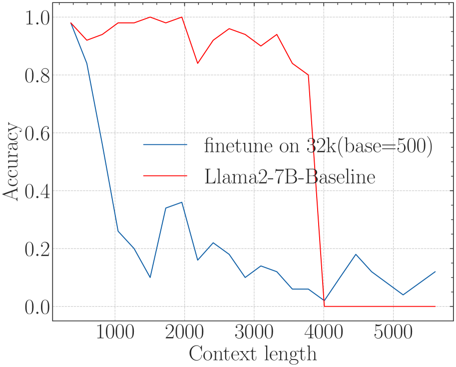
(b) Long-eval (Li* et al., 2023)
<details>
<summary>x7.png Details</summary>
### Visual Description
# Technical Data Extraction: Heatmap Analysis
## 1. Document Overview
This image is a technical heatmap visualization representing the relationship between "Token Limit" and "Context length" relative to a "Score" metric. The chart uses a color gradient to represent numerical values across a two-dimensional grid.
## 2. Component Isolation
### A. Header/Axes Labels
- **Y-Axis Label (Left):** "Context length"
- **X-Axis Label (Bottom):** "Token Limit"
- **Legend Label (Right):** "Score"
### B. Main Chart Area (Data Grid)
The chart consists of a grid where the X-axis represents discrete token intervals and the Y-axis represents context length percentages.
### C. Legend (Color Scale)
- **Location:** Right side of the image.
- **Scale Range:** 0 to 10.
- **Color Mapping:**
- **Teal/Bright Green (Value 10):** High performance/score.
- **Yellow/Light Green (Value 5-7):** Moderate performance/score.
- **Orange/Red (Value 0-3):** Low performance/score.
---
## 3. Axis Markers and Categories
### X-Axis: Token Limit
The axis contains 41 discrete markers ranging from 0 to 4000 in increments of 100:
`0, 100, 200, 300, 400, 500, 600, 700, 800, 900, 1000, 1100, 1200, 1300, 1400, 1500, 1600, 1700, 1800, 1900, 2000, 2100, 2200, 2300, 2400, 2500, 2600, 2700, 2800, 2900, 3000, 3100, 3200, 3300, 3400, 3500, 3600, 3700, 3800, 3900, 4000`
### Y-Axis: Context length
The axis contains 10 markers representing percentages or relative lengths:
`0.0, 11.0, 22.0, 33.0, 44.0, 56.0, 67.0, 78.0, 89.0, 100.0`
---
## 4. Trend Verification and Data Extraction
### General Trends
1. **High Performance Zone (Left):** There is a consistent block of high scores (Teal, ~10) for Token Limits between 0 and 600 across almost all context lengths.
2. **Performance Degradation (Middle-Right):** As the Token Limit increases beyond 900, the scores generally drop into the low range (Red/Orange, ~0-3), with sporadic "islands" of moderate performance.
3. **The "100.0" Context Length Exception:** The bottom-most row (Context length 100.0) maintains a high score (Teal, ~10) across almost the entire Token Limit range, regardless of the horizontal value.
4. **Vertical Strips:** There are vertical bands of consistent color, suggesting that for certain Token Limits (e.g., 1300, 1700-1900, 3100-3700), the score is consistently low regardless of context length (excluding the 100.0 row).
### Specific Data Point Observations (Logic-Check)
* **Token Limit 0-600:** Predominantly Teal (Score 9-10).
* **Token Limit 700-800:** Transition zone, predominantly Light Green (Score 7-8).
* **Token Limit 1300:** Vertical strip of Red (Score ~1-2).
* **Token Limit 2000:** Shows a vertical strip of Yellow/Green (Score ~6-7) amidst a lower-scoring region.
* **Token Limit 3800:** Shows a vertical strip of Yellow (Score ~5-6).
* **Token Limit 4000:** The final column shows a slight improvement to Orange/Yellow compared to the deep Red of the 3100-3700 range.
---
## 5. Reconstructed Data Table (Summary)
| Context Length | Token Limit 0-600 | Token Limit 900-1200 | Token Limit 1300 | Token Limit 3100-3700 | Token Limit 4000 |
| :--- | :--- | :--- | :--- | :--- | :--- |
| **0.0 - 89.0** | High (9-10) | Low-Mid (3-5) | Very Low (1-2) | Very Low (1-2) | Low-Mid (3-5) |
| **100.0** | High (10) | High (10) | High (10) | High (10) | High (10) |
---
## 6. Final Technical Summary
The heatmap illustrates a "short-context" or "low-token" bias where performance is optimal at Token Limits below 700. A significant anomaly exists at the maximum Context Length (100.0), where performance remains high across the entire tested Token Limit spectrum. Conversely, the region between Token Limits 3100 and 3700 represents the lowest performance area for all context lengths except the maximum.
</details>
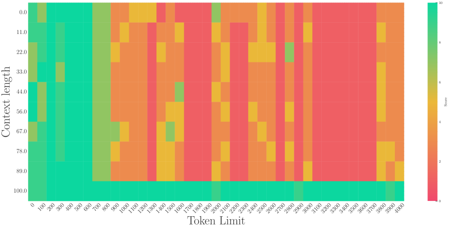
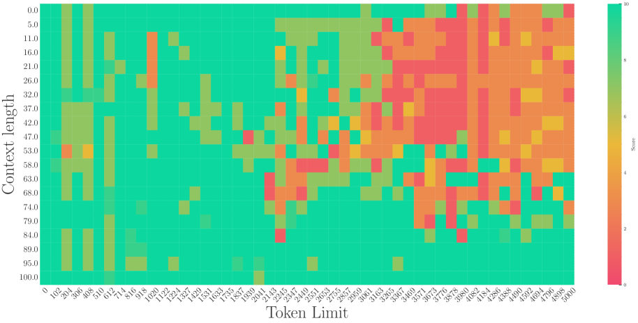
(c) Needle in Haystack (G, 2023)
Figure 3: The superficial long context capability of avoiding OOD by the smaller base. Following the recent work (Liu et al., 2024b), we fine-tune Llama2-7B with a small base (500) to a context length of 32k.
NTK-based methods are widely adopted in long-context extension (Touvron et al., 2023a; Liu et al., 2024a; Young et al., 2024). To obtain better long-context capability, however, practitioners often adopt a much larger base than the original NTK-aware method suggested. This leads to speculation that there is another bound of RoPE’s base determined by context length.
On the other hand, a recent work (Liu et al., 2024b) proposes to set a much smaller base for RoPE to extend the context length. However, we find it may be a superficial long-context capability as shown in Figure 3. This method can obtain a low perplexity even at 128k context length, which can be explained by the OOD theory as explained above, but the model could not retrieve related information for context length as short as 1k, even much shorter than the model’s pre-trained length. Our findings support previous research (Hu et al., 2024) on the limitations of perplexity in evaluating long-context abilities. To delve deep into this phenomenon, we do the theoretical exploration in the next section.
4 Theory Perspective
For attention mechanism in language modeling, we have the following desiderata:
**Desiderata 1**
*The closer token gets more attention: the current token tends to pay more attention to the token that has a smaller relative distance.*
**Desiderata 2**
*The similar token gets more attention: the token tends to pay more attention to the token whose key value is more similar to the query value of the current token.*
Then we examine the desiderata when we apply RoPE to the attention mechanism in LLMs.
4.1 Long-term Decay of Upper Bound of Attention Score
For Desiderata 1, the property of RoPE makes the model attend more to closer tokens. This kind of long-term decay has been thoroughly discussed in previous work (Su et al., 2024; Sun et al., 2022). It comes from the upper bound of attention score calculation, which can be written as:
$$
\displaystyle|A_{ij}|=|q_{i}^{T}R_{m}k_{j}| \displaystyle\leq\max_{l}(|h_{l}-h_{l+1}|)\sum_{n=1}^{d/2}|S_{n}| \displaystyle=\max_{l}(|h_{l}-h_{l+1}|)\sum_{n=1}^{d/2}|\sum_{l=0}^{n-1}e^{(j-i)\theta_{l}\sqrt{-1}}|, \tag{14}
$$
where $h_{l}=q_{i}^{T}[2l:l2+1]k_{j}[2l:2l+1]$ . Equation 4.1 indicates that the upper bound of the attention score $|A_{ij}|$ decays as the relative distance increases. Figure 5 shows the long-term decay curve of this upper bound, which is in accordance with previous findings (Su et al., 2024; Sun et al., 2022).
4.2 Long-term Decay of the Ability to Attend More to Similar Tokens than Random Tokens
In addition to the attention score’s upper bound, we also find there exists another long-term decay property in RoPE: the ability to attend more to similar tokens than random tokens decays as the relative distance increases. We define the ability to attend more to similar tokens than random tokens as:
$$
\displaystyle\mathbb{E}_{q,k^{*}}\left[q^{T}R_{m,\theta}k^{*}\right]-\mathbb{E}_{q,k}\left[q^{T}R_{m,\theta}k\right], \tag{15}
$$
where $q∈ R^{d}$ is the query vector for the current token, $k^{*}=q+\epsilon$ is the key value of a similar token, where $\epsilon$ is a small random variable, $k∈ R^{d}$ is the key vector of a random token, $R_{m,\theta}$ is the rotation matrix in RoPE. The first term in Eq. 15 is the attention score of $q$ and a similar token $k^{*}$ , the second term in Eq. 15 is the attention score of $q$ and random token $k$ . Then we derive the following theorem:
**Theorem 1**
*Assuming that the components of query $q∈ R^{d}$ and key $k∈ R^{d}$ are independent and identically distributed, their standard deviations are denoted as $\sigma∈ R$ . The key $k^{*}=q+\epsilon$ is a token similar to the query, where $\epsilon$ is a random variable with a mean of 0. Then we have:
$$
\displaystyle\frac{1}{2\sigma^{2}}(\mathbb{E}_{q,k^{*}}\left[q^{T}R_{m,\theta}k^{*}\right]-\mathbb{E}_{q,k}\left[q^{T}R_{m,\theta}k\right])=\sum_{i=0}^{d/2-1}\cos(m\theta_{i}) \tag{16}
$$*
<details>
<summary>x8.png Details</summary>
### Visual Description
# Technical Data Extraction: Relative Upper Bound Analysis
This document provides a comprehensive extraction of the data and trends presented in the provided image, which consists of two side-by-side line charts comparing "Relative upper bound" against "Relative distance" for different "base" configurations.
## 1. General Metadata
* **Image Type:** Two-panel line graph.
* **Language:** English.
* **Primary Metrics:**
* **Y-Axis:** Relative upper bound (Linear scale).
* **X-Axis:** Relative distance (Linear scale).
* **Common Legend Format:** `base:1eN` (where N is an integer).
---
## 2. Left Chart Analysis (Short Range)
### Component Isolation
* **Header/Legend:** Located in the top-right quadrant.
* **X-Axis Range:** 0 to 4000. Markers at [0, 2000, 4000].
* **Y-Axis Range:** 2.5 to 15.0. Markers at [2.5, 5.0, 7.5, 10.0, 12.5, 15.0].
### Data Series & Trends
| Series Label | Color | Initial Value (approx.) | Visual Trend Description | Convergence/Steady State |
| :--- | :--- | :--- | :--- | :--- |
| **base:1e4** | Blue | ~16.0 | Sharp exponential decay from 0 to 1000, then stabilizes into a high-frequency oscillation. | Oscillates between ~4.0 and ~6.0. |
| **base:1e2** | Green | ~10.0 | Extremely rapid drop to a floor within the first 100 units of distance. | Oscillates between ~4.0 and ~5.5. |
| **base:1e3** | Orange | ~13.0 | Rapid decay, intersecting the green line at distance ~500. Exhibits the highest amplitude oscillations. | Oscillates between ~3.0 and ~6.5. |
---
## 3. Right Chart Analysis (Long Range)
### Component Isolation
* **Header/Legend:** Located in the top-right quadrant.
* **X-Axis Range:** 0 to 30000+. Markers at [0, 10000, 20000, 30000].
* **Y-Axis Range:** 5 to 15+. Markers at [5, 10, 15].
### Data Series & Trends
| Series Label | Color | Initial Value (approx.) | Visual Trend Description | Convergence/Steady State |
| :--- | :--- | :--- | :--- | :--- |
| **base:1e4** | Blue | ~18.0 | Rapid decay. In this wider view, it maintains the lowest baseline of the three series. | Oscillates between ~3.5 and ~6.0. |
| **base:1e5** | Green | ~15.0 | Moderate decay. Stays consistently between the blue and orange lines. | Oscillates between ~4.0 and ~7.0. |
| **base:1e6** | Orange | ~18.0 | Slowest decay relative to the others. Maintains the highest average bound across the distance. | Oscillates between ~5.0 and ~8.0. |
---
## 4. Comparative Summary and Key Findings
### Trend Verification
1. **Initial Penalty:** All configurations start with a high "Relative upper bound" at distance 0, which decays as distance increases.
2. **Base Value Correlation:**
* In the **Left Chart** (lower base values), the `base:1e4` (highest in that set) has the slowest decay and highest initial bound.
* In the **Right Chart** (higher base values), the `base:1e6` (highest in that set) has the slowest decay and maintains the highest bound over long distances.
* **Conclusion:** Increasing the "base" value generally increases the relative upper bound and slows the rate of decay toward the steady-state oscillation.
3. **Oscillatory Behavior:** All series transition from a smooth decay curve into a "noisy" or oscillatory steady state. The amplitude of these oscillations appears more pronounced in the `base:1e3` (Left) and `base:1e6` (Right) configurations.
### Spatial Grounding of Legends
* **Left Plot Legend [x~0.7, y~0.8]:** Correctly identifies Blue (1e4), Green (1e2), and Orange (1e3).
* **Right Plot Legend [x~0.7, y~0.8]:** Correctly identifies Blue (1e4), Green (1e5), and Orange (1e6). Note that Blue (1e4) is the common reference point between both charts.
</details>
Figure 4: The upper bound of attention score with respect to the relative distance.
<details>
<summary>x9.png Details</summary>
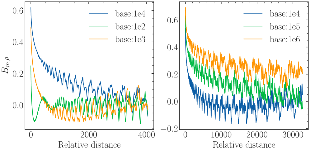
### Visual Description
# Technical Data Extraction: Rotary Positional Embedding (RoPE) Decay Analysis
This document provides a detailed technical extraction of the data presented in the two-panel line chart. The charts illustrate the relationship between "Relative distance" and a metric labeled $B_{m, \theta}$, likely representing the decay of basis functions or attention scores in a transformer model using different "base" values for positional encoding.
---
## 1. Global Metadata and Layout
* **Image Type:** Two-panel line plot (Left and Right).
* **Primary Language:** English.
* **Y-Axis Label (Shared):** $B_{m, \theta}$
* **X-Axis Label (Shared):** Relative distance
* **Visual Style:** Scientific plot with LaTeX-style font rendering.
---
## 2. Left Panel Analysis (Short Range)
### Axis Scales
* **X-Axis Range:** 0 to 4000. Major ticks at 0, 2000, 4000.
* **Y-Axis Range:** -0.2 to 0.6. Major ticks at 0.0, 0.2, 0.4, 0.6.
### Legend and Data Series [Spatial Grounding: Top Right Quadrant]
| Series Color | Label | Trend Description |
| :--- | :--- | :--- |
| **Blue** | `base:1e4` | Starts highest (~0.62). Slopes downward with high-frequency oscillations. Remains above other series until ~3500. |
| **Orange** | `base:1e3` | Starts at ~0.5. Rapidly decays to near 0.0 by distance 1000, then oscillates around the 0.0 axis. |
| **Green** | `base:1e2` | Starts lowest (~0.25). Drops sharply into negative values (~ -0.1) before distance 500, then oscillates around 0.0. |
### Key Observations
* Higher base values (1e4) maintain a higher $B_{m, \theta}$ value over longer relative distances.
* Lower base values (1e2, 1e3) exhibit much faster initial decay and settle into a zero-centered oscillation pattern much earlier.
---
## 3. Right Panel Analysis (Long Range)
### Axis Scales
* **X-Axis Range:** 0 to 30,000+. Major ticks at 0, 10000, 20000, 30000.
* **Y-Axis Range:** -0.2 to 0.6 (consistent with left panel).
### Legend and Data Series [Spatial Grounding: Top Right Quadrant]
| Series Color | Label | Trend Description |
| :--- | :--- | :--- |
| **Orange** | `base:1e6` | Starts highest (~0.65). Slopes downward gradually, maintaining the highest mean value (~0.25) at distance 30,000. |
| **Green** | `base:1e5` | Starts middle (~0.55). Slopes downward, maintaining a mean value around 0.1 at distance 30,000. |
| **Blue** | `base:1e4` | Starts lowest (~0.45 on this scale). Slopes downward rapidly, oscillating around 0.0 by distance 10,000. |
### Key Observations
* This panel focuses on much larger relative distances (up to 32k).
* The `base:1e4` series, which was the "high" performer in the left plot, is the "low" performer here, showing that base values must scale with the intended context window to prevent the metric from decaying to zero.
* All series exhibit a "fuzzy" appearance caused by high-frequency oscillations superimposed on the general downward decay curve.
---
## 4. Comparative Summary Table
| Base Value | Initial Value ($B_{m, \theta}$) | Effective Range (before mean $\approx$ 0) |
| :--- | :--- | :--- |
| **1e2** | ~0.25 | < 500 |
| **1e3** | ~0.50 | ~1,000 |
| **1e4** | ~0.62 | ~8,000 - 10,000 |
| **1e5** | ~0.55 | > 32,000 (Mean remains > 0) |
| **1e6** | ~0.65 | > 32,000 (Mean remains ~0.2) |
**Conclusion:** Increasing the `base` parameter significantly extends the distance over which the $B_{m, \theta}$ metric remains positive and significant, effectively "stretching" the positional encoding's reach.
</details>
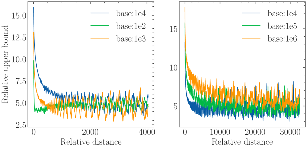
Figure 5: The ability to attend more to similar tokens than random tokens.
The proof is shown in Appendix A. We denote $\sum_{i=0}^{d/2-1}\cos(m\theta_{i})$ as $B_{m,\theta}$ , and according to Theorem 1, $B_{m,\theta}$ measures the ability to give more attention to similar tokens than random tokens, which decreases as the relative distance $m$ increases, as shown in Figure 5. For a very small base value, we can observe that the $B_{m,\theta}$ is even below zero at a certain distance, meaning the random tokens have larger attention scores than the similar tokens, which may be problematic for long context modeling.
4.3 Base of RoPE Bounds the Context Length
To satisfy the Desiderata 2, we will get $\mathbb{E}_{q,k^{*}}\left[q^{T}R_{m,\theta}k^{*}\right]≥\mathbb{E}_{q,k}\left[q^{T}R_{m,\theta}k\right]$ . According to Theorem 1, $B_{m,\theta}$ needs to be larger than zero. Given the $\theta$ in RoPE, the context length $L_{\theta}$ that can be truly obtained satisfies:
$$
\displaystyle L_{\theta}=\sup\{L|B_{m,\theta}\geq 0,\forall m\in[0,1,...,L]\} \tag{17}
$$
In other word, if we follow the setting that $\theta_{i}=base^{-2i/d}$ , in order to get the expected context length $L$ , there is a lower bound of the base value $base_{L}$ :
$$
\displaystyle base_{L}=\inf\{base|B_{m,\theta}\geq 0,\forall m\in[0,1,...,L]\} \tag{18}
$$
In summary, the RoPE’s base determines the upper bound of context length the model can truly obtain. Although there exists the absolute lower bound, Eq. 16 and Eq. 18 are hard to get the closed-form solution since $B_{m,\theta}$ is a summation of many cosine functions. Therefore, in this paper, we get the numerical solution. Table 2 shows this lower bound for context length ranging from 1,000 to one million. In Figure 1, we plot the context length and corresponding lower bound, we can observe that as the context length increases, the required base also increases.
Table 2: Context length and its corresponding lower bound of RoPE’s base.
| Context Len. Lower Bound | 1k 4.3e3 | 2k 1.6e4 | 4k 2.7e4 | 8k 8.4e4 | 16k 3.1e5 | 32k 6.4e5 | 64k 2.1e6 | 128k 7.8e6 | 256k 3.6e7 | 512k 6.4e7 | 1M 5.1e8 |
| --- | --- | --- | --- | --- | --- | --- | --- | --- | --- | --- | --- |
Note: this boundary is not very strict because the stacking of layers in LLMs allows the model to extract information beyond the single layers’ range, which may increase the context length in Eq. 17 and decrease the base in Eq. 18. Notwithstanding, in Section 5 we find that the derived bound approximates the real context length in practice.
Long-term decay from different perspectives. The long-term decay in section 4.1 and section 4.2 are from different perspectives. The former refers to the long-term decay of the attention score as the relative distance increases. This ensures that current tokens tend to pay more attention to the tokens closer to them. The latter indicates that with the introduction of the rotation matrix in attention, the ability to discriminate the relevant tokens from irrelevant tokens decreases as the relative distance increases. Therefore, a large $B_{m,\theta}$ , corresponding to a large base value, is important to keep the model’s discrimination ability in long context modeling.
5 Experiment
In this section, we conduct thorough experiments. The empirical result can be summarized in Table 3, the details are in the following sections.
Table 3: In Section 5, we aim to answer the following questions.
| Q: Does RoPE’s base bounds the context length during the fine-tuning stage? | Yes. When the base is small, it is difficult to get extrapolation for specific context length. |
| --- | --- |
| Q: Does RoPE’s base bounds the context length during the pre-training stage? | Yes. Our proposed lower bound for RoPE’s base also applies to pre-training. If we train a model from scratch with a small base but the context length is large (larger than the bounded length), the resulting model has very limited the context length capabilities, meaning some of context in pre-training is wasted. |
| Q: What happened when base is set smaller than the lower bound? | The model will get the superficial long context capability. The model can keep perplexity low, but can’t retrieve useful information from long context. |
5.1 Experiments Setup
For fine-tuning, we utilized Llama2-7B (Touvron et al., 2023a) and Baichuan2-7B (Yang et al., 2023), both of which are popular open-source models employing RoPE with a base of $1e4$ . We utilized a fixed learning rate of 2e-5 and a global batch size of 128 and fine-tuning for 1000 steps. For pre-training, we trained a Llama-like 2B model from scratch for a total of 1 trillion tokens. We set the learning rate to 1e-4 and adopted a cosine decay schedule, with models trained on a total of 1T tokens. The dataset we used is a subset of RedPajama (Computer, 2023). More details of the experimental setup are provided in Appendix B.
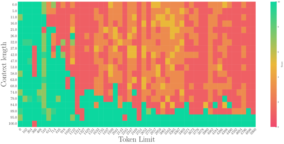
Our evaluation focused on two aspects: (1) Perplexity: we use PG19 dataset (Rae et al., 2019) which are often used in long context evaluation; (2) Retrieval: in addition to perplexity, we also adopt retrieval since it represents the real long-context understanding ability of LLMs. We choose a) Long-eval benchmark from (Li* et al., 2023) and b) needle in a haystack (NIH) (G, 2023). The Long-eval benchmark generates numerous random similar sentences and asks the model to answer questions based on a specific sentence within the context, while the NIH requires the model to retrieve information from various positions in the long context.
5.2 Base of RoPE bounds context length in fine-tuning stages
<details>
<summary>x10.png Details</summary>
### Visual Description
# Technical Data Extraction: Perplexity vs. Context Length Chart
## 1. Image Overview
This image is a line graph illustrating the relationship between **Context** (x-axis) and **Perplexity** (y-axis) for various configurations of a language model. The chart compares a baseline model with a 4K context window against several models configured with a 32K context window using different "base" parameters.
## 2. Component Isolation
### A. Header/Metadata
* **Language:** English.
* **Content:** No explicit title is present within the image frame.
### B. Main Chart Area
* **Y-Axis Label:** Perplexity
* **Y-Axis Scale:** Linear, ranging from 5 to 20. Major tick marks are placed at intervals of 2 (6, 8, 10, 12, 14, 16, 18, 20).
* **X-Axis Label:** Context
* **X-Axis Scale:** Linear, ranging from 5,000 to 30,000. Major tick marks are placed at intervals of 5,000 (5000, 10000, 15000, 20000, 25000, 30000).
* **Grid:** Horizontal and vertical dashed light-gray grid lines corresponding to the major tick marks.
### C. Legend (Spatial Grounding: Top-Right Quadrant)
The legend is located at approximately `[x=0.65 to 0.95, y=0.05 to 0.50]` in normalized coordinates from the top-left. It contains seven entries:
1. **Blue line:** `32K-base:1e4`
2. **Green line:** `32K-base:2e5`
3. **Orange line:** `32K-base:9e5`
4. **Red line:** `32K-base:5e6`
5. **Purple line:** `32K-base:1e9`
6. **Dark Gray/Black line:** `32K-base:1e12`
7. **Light Gray line:** `4K-Baseline`
---
## 3. Trend Verification and Data Extraction
### Series 1: 4K-Baseline (Light Gray)
* **Trend:** Sharp exponential upward slope. The perplexity explodes almost immediately after the 5,000 context mark.
* **Data Points:**
* At Context 5,000: ~8.2
* At Context 6,000: ~10.2
* At Context 7,500: Exceeds 20.0 (off-chart).
### Series 2: 32K-base Group (Multiple Colors)
* **Trend:** All 32K-base models follow a nearly identical, stable horizontal trend. They maintain low perplexity (between 8 and 10) across the entire context range shown (5,000 to 31,000). There is a very slight, gradual increase in perplexity as context increases, with a small "hump" or local peak around Context 19,000.
* **Detailed Comparison:**
* **32K-base:1e4 (Blue):** Generally the highest perplexity among the 32K group, ending near 9.5 at Context 31,000.
* **32K-base:1e12 (Dark Gray):** Closely follows the blue line.
* **32K-base:5e6 (Red):** Generally the lowest perplexity among the 32K group, ending near 9.0 at Context 31,000.
* **Representative Data Points (Approximate Average of Group):**
* Context 5,000: ~8.1
* Context 10,000: ~8.3
* Context 15,000: ~8.2
* Context 19,000: ~8.8 (Local peak)
* Context 25,000: ~8.7
* Context 31,000: ~9.1 to 9.5
---
## 4. Summary Table of Extracted Data
| Context Length | 4K-Baseline Perplexity | 32K-base (Group Avg) Perplexity |
| :--- | :--- | :--- |
| 5,000 | ~8.2 | ~8.1 |
| 7,500 | > 20.0 | ~8.4 |
| 10,000 | N/A (Off-chart) | ~8.3 |
| 15,000 | N/A | ~8.2 |
| 20,000 | N/A | ~8.7 |
| 25,000 | N/A | ~8.7 |
| 30,000 | N/A | ~9.2 |
## 5. Technical Conclusion
The chart demonstrates that the **4K-Baseline** model fails to generalize beyond its training window, as evidenced by the vertical spike in perplexity after 5,000 context tokens. Conversely, all **32K-base** variants (ranging from 1e4 to 1e12) successfully maintain performance (low perplexity) up to at least 31,000 context tokens, with only marginal differences between the specific base configurations.
</details>
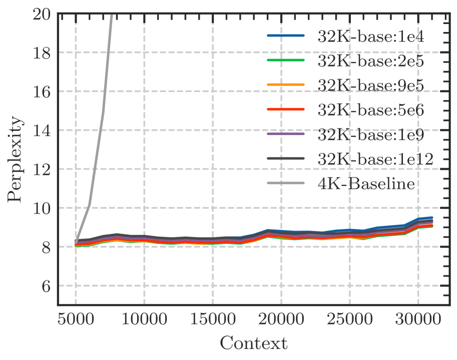
(a) Perplexity
<details>
<summary>x11.png Details</summary>
### Visual Description
# Technical Data Extraction: Accuracy vs. Base Value Chart
## 1. Component Isolation
* **Header:** None present.
* **Main Chart Area:** A 2D line plot with a grid, featuring one data series (teal line with star markers) and one reference line (dark blue dash-dotted vertical line).
* **Legend:** Located in the bottom-right quadrant.
* **Axes:** X-axis (Base value) and Y-axis (Accuracy on 32K).
## 2. Axis Specifications
* **Y-Axis (Vertical):**
* **Label:** "Accuracy on 32K"
* **Scale:** Linear, ranging from 0.0 to 0.4 (topmost visible tick is 0.3, but the grid extends higher).
* **Major Markers:** 0.0, 0.1, 0.2, 0.3.
* **X-Axis (Horizontal):**
* **Label:** "Base value"
* **Scale:** Logarithmic/Non-linear (based on scientific notation labels).
* **Major Markers:** 1e4, 2e5, 9e5, 5e6, 1e9, 1e12.
## 3. Legend and Reference Lines
* **Legend Location:** [x=0.7, y=0.1] (Bottom-right).
* **Legend Item:**
* **Symbol:** Dark blue dash-dotted line (`- . -`).
* **Label:** "Lower bound".
* **Reference Line Placement:** A vertical dark blue dash-dotted line is positioned exactly at the x-axis value of **9e5**.
## 4. Data Series Analysis (Teal Line)
* **Color:** Teal / Cyan.
* **Marker:** 5-point star.
* **Trend Verification:** The line shows a sharp upward slope from 1e4 to 5e6, reaching a peak. It then experiences a slight dip at 1e9 before recovering to a high plateau at 1e12.
### Extracted Data Points (Estimated from Grid)
| Base value (X) | Accuracy on 32K (Y) | Notes |
| :--- | :--- | :--- |
| 1e4 | ~0.00 | Starting point at origin. |
| 2e5 | ~0.06 | Initial slow growth. |
| ~5e5 | ~0.17 | Sharp increase (unlabeled tick). |
| 9e5 | ~0.27 | Intersects the "Lower bound" vertical line. |
| ~2e6 | ~0.33 | Continued sharp growth. |
| 5e6 | ~0.35 | Local maximum/peak. |
| 1e9 | ~0.30 | Notable performance dip. |
| 1e12 | ~0.35 | Recovery to peak performance level. |
## 5. Summary of Findings
The chart illustrates the relationship between a "Base value" and "Accuracy on 32K". Performance is negligible at low base values (1e4) but improves rapidly as the value approaches **9e5**, which is explicitly marked as a "Lower bound." The accuracy peaks around **5e6**, remains relatively stable despite a minor fluctuation at **1e9**, and finishes at its highest recorded accuracy (approx. 0.35) at a base value of **1e12**.
</details>
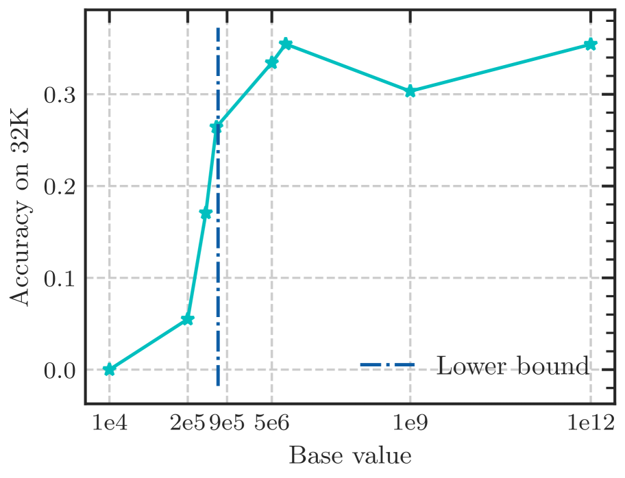
(b) Long-eval 32k
Figure 6: Fine-tuning Llama2-7B-Base on 32k context length with varying RoPE’s base. Although the perplexity remains low with varying bases, the Long-eval accuracy reveals a discernible bound for the base value, below which the Long-eval accuracy declines significantly. The dotted line denotes the lower bound derived from Eq. 18.
According to Eq. 18, there is a lower bound of RoPE’s base determined by expected context length. We fine-tune Llama2-7b-Base on 32k context with varying bases. As depicted in Figure 6, although the difference in perplexity between different bases is negligible, the accuracy of Long-eval varies significantly. In Figure 6(b), the dotted line denotes the lower bound derived from Eq. 18, below which the Long-eval accuracy declines significantly. Additional results are provided in Appendix C. Notably, this empirically observed lower bound closely aligns with our theoretical derivation. On the other hand, we can see that $base=2e5$ achieves the best perplexity, but the accuracy of Long-eval is very low, which indicates the limitations of perplexity in evaluating long context capabilities.
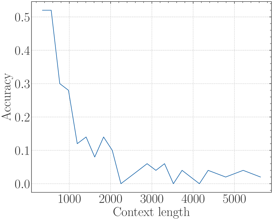
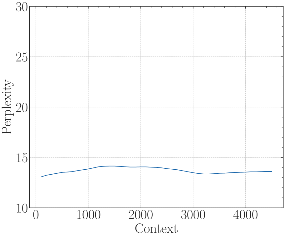
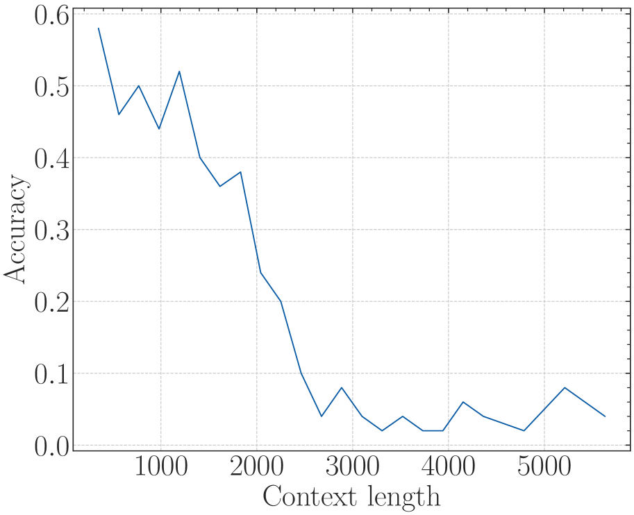
5.3 The Base of RoPE bounds context length in pre-training stages
<details>
<summary>x12.png Details</summary>
### Visual Description
# Technical Document Extraction: Perplexity vs. Context Chart
## 1. Image Classification and Overview
This image is a line chart depicting the relationship between "Context" (independent variable) and "Perplexity" (dependent variable). The chart is presented in a clean, academic style with a grid background.
## 2. Component Isolation
### Header/Title
* **Content:** None present.
### Main Chart Area
* **Background:** White with a light gray dashed grid.
* **Grid Lines:** Vertical and horizontal dashed lines corresponding to major axis ticks.
* **Data Series:** A single solid line in a dark blue/teal color.
### Axis Labels and Markers
* **Y-Axis (Vertical):**
* **Label:** "Perplexity" (oriented vertically).
* **Range:** 10 to 30.
* **Major Ticks:** 10, 15, 20, 25, 30.
* **Minor Ticks:** Present between major ticks (unlabeled).
* **X-Axis (Horizontal):**
* **Label:** "Context".
* **Range:** 0 to approximately 4500.
* **Major Ticks:** 0, 1000, 2000, 3000, 4000.
* **Minor Ticks:** Present at intervals of 500 (unlabeled).
### Legend
* **Location:** None present. As there is only one data series, the line color is the primary identifier.
---
## 3. Data Extraction and Trend Analysis
### Trend Verification
The data series (Dark Blue Line) exhibits a non-linear trend:
1. **Initial Phase (0 - 200):** Starts at approximately 11.2, dips slightly, then begins to rise.
2. **Growth Phase (200 - 2500):** The line slopes upward steadily, showing a positive correlation between Context and Perplexity.
3. **Plateau Phase (2500 - 3500):** The line flattens out, reaching its peak value.
4. **Slight Decline/Stabilization (3500 - 4500):** The line shows a very slight downward trend before leveling off at the end of the recorded range.
### Estimated Data Points
Based on the visual alignment with the grid and axis markers:
| Context (X) | Perplexity (Y) | Notes |
| :--- | :--- | :--- |
| ~100 | ~11.2 | Starting point |
| 500 | ~11.8 | Steady climb |
| 1000 | ~12.7 | |
| 1500 | ~13.5 | |
| 2000 | ~14.1 | Approaching plateau |
| 2500 | ~14.4 | Peak region |
| 3000 | ~14.4 | Peak region |
| 3500 | ~14.3 | Slight dip |
| 4000 | ~14.1 | |
| 4500 | ~14.1 | Final data point |
---
## 4. Summary of Information
The chart illustrates that as the **Context** increases from 0 to roughly 2500, the **Perplexity** increases from approximately 11 to 14.4. Beyond a Context value of 2500, the Perplexity stabilizes and remains relatively constant between 14.0 and 14.5 through to the Context value of 4500. This suggests a "saturation" point where additional context no longer significantly impacts the perplexity metric in the same upward trajectory.
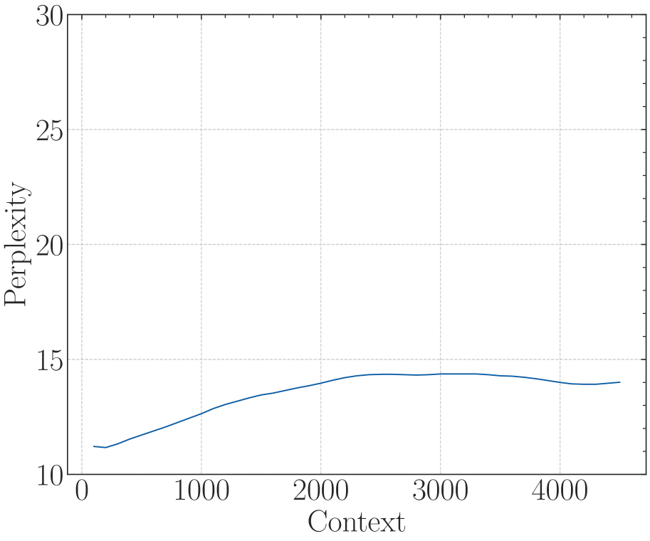
</details>
<details>
<summary>x13.png Details</summary>
### Visual Description
# Technical Data Extraction: Accuracy vs. Context Length
## 1. Image Classification
This image is a **line chart** depicting the relationship between a model's performance (Accuracy) and the length of the input context (Context length).
## 2. Component Isolation
### Header/Metadata
* **Title:** None present.
* **Language:** English.
### Main Chart Area
* **X-Axis Label:** "Context length"
* **Y-Axis Label:** "Accuracy"
* **Grid:** Light gray dashed grid lines for both major x and y intervals.
* **Data Series:** A single solid blue line.
### Legend
* **Presence:** No legend is present as there is only one data series.
---
## 3. Axis Scales and Markers
### X-Axis (Context length)
* **Range:** Approximately 400 to 5800.
* **Major Tick Labels:** 1000, 2000, 3000, 4000, 5000.
* **Minor Ticks:** Present between major labels, indicating intervals of 200 units.
### Y-Axis (Accuracy)
* **Range:** 0.0 to 0.55.
* **Major Tick Labels:** 0.0, 0.1, 0.2, 0.3, 0.4, 0.5.
* **Minor Ticks:** Present at intervals of 0.025.
---
## 4. Trend Verification and Data Extraction
### Visual Trend Analysis
The blue line exhibits a **sharp negative correlation** initially, followed by a **volatile plateau** at low values.
1. **Initial Phase (400 - 1200):** The line starts at its peak and drops precipitously.
2. **Transition Phase (1200 - 2200):** The line fluctuates with a downward bias, showing small "sawtooth" peaks.
3. **Degraded Phase (2200 - 5600):** The line remains near the baseline (0.0 to 0.06), oscillating frequently and hitting 0.0 at multiple points.
### Estimated Data Points
Based on the grid intersections and axis markers:
| Context length (approx.) | Accuracy (approx.) | Notes |
| :--- | :--- | :--- |
| 400 | 0.52 | Peak performance |
| 600 | 0.52 | Performance holds |
| 800 | 0.30 | Sharp drop |
| 1000 | 0.28 | Continued decline |
| 1200 | 0.12 | Local minimum |
| 1400 | 0.14 | Small recovery |
| 1600 | 0.08 | Local minimum |
| 1800 | 0.14 | Local peak |
| 2000 | 0.10 | Decline |
| 2200 | 0.00 | First zero-accuracy point |
| 2800 | 0.06 | Small recovery |
| 3000 | 0.04 | Decline |
| 3200 | 0.06 | Small recovery |
| 3500 | 0.00 | Second zero-accuracy point |
| 3700 | 0.04 | Small recovery |
| 4100 | 0.00 | Third zero-accuracy point |
| 4300 | 0.04 | Small recovery |
| 4800 | 0.02 | Decline |
| 5200 | 0.04 | Small recovery |
| 5600 | 0.02 | Final data point |
---
## 5. Summary of Findings
The chart demonstrates a significant degradation in model accuracy as the context length increases. The model maintains its highest accuracy (~0.52) only for very short contexts (under 600 units). By the time the context length reaches 2200 units, the accuracy effectively collapses, frequently hitting 0.0 and never recovering above 0.06 for the remainder of the tested range (up to 5600 units).
</details>
<details>
<summary>x14.png Details</summary>
### Visual Description
# Technical Data Extraction: Performance Heatmap
## 1. Document Overview
This image is a technical heatmap visualization representing the relationship between "Context length" and "Token Limit" on a numerical "Score." The chart uses a color gradient to represent performance metrics, where green indicates high scores and red indicates low scores.
## 2. Component Isolation
### A. Header / Metadata
* **Language:** English.
* **Content:** No explicit title text is present at the top of the image.
### B. Main Chart (Heatmap)
* **Type:** 2D Heatmap / Grid.
* **Y-Axis Label:** Context length (Vertical, left side).
* **X-Axis Label:** Token Limit (Horizontal, bottom).
* **Color Scale (Legend):** Located on the far right [x=950, y=500 approx.]. It is a vertical gradient bar labeled "Score".
### C. Axis Scales and Markers
#### Y-Axis (Context length)
The axis represents a percentage or ratio from 0.0 to 100.0, with markers every ~5.0 to 6.0 units:
`0.0, 5.0, 11.0, 16.0, 21.0, 26.0, 32.0, 37.0, 42.0, 47.0, 53.0, 58.0, 63.0, 68.0, 74.0, 79.0, 84.0, 89.0, 95.0, 100.0`
#### X-Axis (Token Limit)
The axis represents a count from 0 to 5000, with markers at irregular intervals (roughly every 102 units):
`0, 102, 204, 306, 408, 510, 612, 714, 816, 918, 1020, 1122, 1224, 1327, 1429, 1531, 1633, 1735, 1837, 1939, 2041, 2143, 2245, 2347, 2449, 2551, 2653, 2755, 2857, 2959, 3061, 3163, 3265, 3367, 3469, 3571, 3673, 3776, 3878, 3980, 4082, 4184, 4286, 4388, 4490, 4592, 4694, 4796, 4898, 5000`
## 3. Legend and Color Mapping
* **Score 10 (Bright Green):** Optimal performance.
* **Score 5-7 (Yellow/Orange):** Moderate/Degraded performance.
* **Score 0 (Red/Pink):** Failure or lowest performance.
## 4. Trend Verification and Data Analysis
### Visual Trend Analysis
1. **High Performance Zone (Green):** Concentrated in the bottom-left corner and along the bottom edge. As "Context length" increases (moving down the Y-axis), the system maintains high scores for longer "Token Limits."
2. **Degradation Zone (Red/Orange):** Concentrated in the top-right quadrant. As "Token Limit" increases while "Context length" remains low (top of the chart), performance drops significantly.
3. **The "Diagonal" Boundary:** There is a visible diagonal threshold. When `Context length` is low (e.g., 0.0 - 21.0), performance drops to red almost immediately after a Token Limit of ~510. When `Context length` is high (e.g., 95.0 - 100.0), performance remains green across almost the entire Token Limit range (0 to 5000).
### Key Data Observations
* **Low Context Length (0.0 - 16.0):** Performance is high (Green) only for very small Token Limits (< 510). Beyond 612, the score drops to Red (0-2) with scattered Orange (4-5) noise.
* **Mid Context Length (47.0 - 68.0):** Performance stays high (Green) up to a Token Limit of approximately 1020. Beyond this, it transitions into a "noisy" field of Red and Orange.
* **High Context Length (89.0 - 100.0):** Performance is consistently high (Green) across nearly the entire X-axis. There are very few "failure" pixels (Red), notably one at `Context length 100.0 / Token Limit 306`.
* **The "Noise" Pattern:** In the upper-right region (Token Limit > 2000, Context length < 50), the data is not solid red but "speckled" with orange and yellow, suggesting inconsistent or stochastic performance rather than total failure.
## 5. Summary of Findings
The chart demonstrates an inverse relationship between the two variables regarding performance stability. The system performs best when the **Context length** is high (near 100.0), regardless of the **Token Limit**. Conversely, when the Context length is low, the system can only handle very small Token Limits before the Score degrades to near zero.
</details>
<details>
<summary>x15.png Details</summary>
### Visual Description
# Technical Document Extraction: Perplexity vs. Context Chart
## 1. Component Isolation
* **Header:** None present.
* **Main Chart Area:** A line graph plotted on a Cartesian coordinate system with a light-gray dashed grid.
* **Footer/Axes:** Contains the X-axis label "Context" and the Y-axis label "Perplexity".
## 2. Axis Identification and Markers
* **Y-Axis (Vertical):**
* **Label:** Perplexity
* **Range:** 10 to 30
* **Major Tick Marks:** 10, 15, 20, 25, 30
* **Orientation:** Text is rotated 90 degrees counter-clockwise.
* **X-Axis (Horizontal):**
* **Label:** Context
* **Range:** 0 to approximately 4500+
* **Major Tick Marks:** 0, 1000, 2000, 3000, 4000
* **Minor Tick Marks:** Present at intervals of 500 (unlabeled).
## 3. Data Series Analysis
The chart contains a single data series represented by a solid dark blue line.
### Trend Verification
* **Initial Phase (0 - 1500 Context):** The line shows a steady upward slope, starting slightly above 13 and peaking near 14.2.
* **Middle Phase (1500 - 3200 Context):** The line exhibits a gradual decline, dipping back toward the 13.5 mark.
* **Final Phase (3200 - 4500 Context):** The line stabilizes and shows a very slight upward recovery, ending just below the 14 mark.
* **Overall Stability:** The data remains remarkably stable within a narrow band between 13 and 14.5 perplexity across the entire context window.
### Extracted Data Points (Approximate)
Based on the visual alignment with the grid:
| Context (X) | Perplexity (Y) |
| :--- | :--- |
| 100 | ~13.1 |
| 500 | ~13.5 |
| 1000 | ~13.8 |
| 1500 | ~14.2 (Peak) |
| 2000 | ~14.1 |
| 2500 | ~13.9 |
| 3200 | ~13.4 (Local Minimum) |
| 4000 | ~13.6 |
| 4500 | ~13.7 |
## 4. Visual Style and Metadata
* **Grid:** Light gray dashed lines for both major and minor increments.
* **Font:** Serif typeface used for all labels and numbers.
* **Legend:** No legend is present, as there is only one data series.
* **Language:** English.
## 5. Summary of Information
This technical chart illustrates the relationship between "Context" and "Perplexity." In the field of natural language processing, this typically represents how a model's predictive performance (Perplexity) changes as the input sequence length (Context) increases. The data indicates that the model maintains a consistent perplexity level (between 13 and 14.5) regardless of context length up to 4500 units, suggesting high stability and sustained performance over long sequences.
</details>
<details>
<summary>x16.png Details</summary>
### Visual Description
# Technical Document Extraction: Accuracy vs. Context Length Chart
## 1. Component Isolation
* **Header:** None present.
* **Main Chart Area:** A line graph plotted on a Cartesian coordinate system with a light gray dashed grid.
* **Footer/Axes:** Contains the X-axis label "Context length" and the Y-axis label "Accuracy".
## 2. Axis and Label Extraction
* **Y-Axis (Vertical):**
* **Label:** Accuracy
* **Scale:** 0.0 to 0.6
* **Major Tick Markers:** 0.0, 0.1, 0.2, 0.3, 0.4, 0.5, 0.6
* **X-Axis (Horizontal):**
* **Label:** Context length
* **Scale:** Approximately 400 to 5600
* **Major Tick Markers:** 1000, 2000, 3000, 4000, 5000
## 3. Data Series Analysis
### Trend Verification
The data series is represented by a single solid blue line.
* **Initial Phase (400 - 1200):** The line shows high volatility but maintains a relatively high accuracy between 0.45 and 0.58.
* **Degradation Phase (1200 - 2600):** The line shows a sharp, consistent downward slope, indicating a significant loss in accuracy as context length increases.
* **Baseline Phase (2600 - 5600):** The line flattens out, oscillating at a very low accuracy level (near 0.0 to 0.08), suggesting the model has reached a floor or "noise" level.
### Data Point Extraction (Estimated)
Based on the grid intersections and axis markers, the following data points are extracted:
| Context Length (X) | Accuracy (Y) |
| :--- | :--- |
| ~400 | 0.58 |
| ~600 | 0.46 |
| ~800 | 0.50 |
| ~1000 | 0.44 |
| ~1200 | 0.52 |
| ~1400 | 0.40 |
| ~1600 | 0.36 |
| ~1800 | 0.38 |
| ~2000 | 0.24 |
| ~2200 | 0.20 |
| ~2400 | 0.10 |
| ~2600 | 0.04 |
| ~2800 | 0.08 |
| ~3000 | 0.04 |
| ~3200 | 0.02 |
| ~3400 | 0.04 |
| ~3600 | 0.02 |
| ~3800 | 0.02 |
| ~4000 | 0.06 |
| ~4200 | 0.04 |
| ~4400 | 0.03 |
| ~4600 | 0.02 |
| ~4800 | 0.05 |
| ~5000 | 0.08 |
| ~5200 | 0.06 |
| ~5400 | 0.04 |
## 4. Summary of Findings
The chart illustrates a strong inverse relationship between "Context length" and "Accuracy". The performance of the system/model is highest at short context lengths (under 1200 units). A critical performance "cliff" occurs between context lengths of 1800 and 2600, where accuracy drops from approximately 38% to nearly 4%. Beyond a context length of 3000, the accuracy remains consistently low, failing to recover significantly.
</details>
<details>
<summary>x17.png Details</summary>
### Visual Description
# Technical Data Extraction: Performance Heatmap Analysis
## 1. Document Overview
This image is a technical heatmap visualizing the relationship between two variables—**Context length** and **Token Limit**—and their impact on a numerical **Score**. The chart uses a color gradient to represent performance levels across a grid of data points.
## 2. Component Isolation
### A. Header/Axes Labels
* **Y-Axis Label (Left):** "Context length"
* **X-Axis Label (Bottom):** "Token Limit"
* **Legend Label (Right):** "Score"
### B. Legend and Scale (Spatial Grounding: [x=right, y=center])
The legend is a vertical color bar on the right side of the chart.
* **Scale Range:** 0 to 10.
* **Color Mapping:**
* **10 (Top - Teal/Green):** Represents the highest score/optimal performance.
* **5-7 (Middle - Yellow/Light Green):** Represents moderate performance.
* **0 (Bottom - Red/Pink):** Represents the lowest score/poor performance.
### C. Axis Markers (Data Categories)
* **Y-Axis (Context length):** 20 intervals ranging from **0.0** to **100.0** (increments of approximately 5.3 units).
* Values: 0.0, 5.0, 11.0, 16.0, 21.0, 26.0, 32.0, 37.0, 42.0, 47.0, 53.0, 58.0, 63.0, 68.0, 74.0, 79.0, 84.0, 89.0, 95.0, 100.0.
* **X-Axis (Token Limit):** 50 intervals ranging from **0** to **5000** (increments of 102 units).
* Key markers: 0, 102, 204, 306, 408, 510, 612, 714, 816, 918, 1020, 1122, 1224, 1327, 1429, 1531, 1633, 1735, 1837, 1939, 2041, 2143, 2245, 2347, 2449, 2551, 2653, 2755, 2857, 2959, 3061, 3163, 3265, 3367, 3469, 3571, 3673, 3776, 3878, 3980, 4082, 4184, 4286, 4388, 4490, 4592, 4694, 4796, 4898, 5000.
---
## 3. Trend Verification and Data Analysis
### Visual Trend Description
The heatmap shows a distinct performance degradation (shifting from teal to red) as both the **Token Limit** and **Context length** increase, though the Token Limit appears to be the primary driver of failure.
1. **High Performance Zone (Teal):** Dominates the left side of the chart (Token Limit < 2000) and the bottom-left quadrant.
2. **Transition Zone (Yellow/Orange):** Appears as a diagonal "noise" pattern starting around Token Limit 2143.
3. **Low Performance Zone (Red/Pink):** Concentrated in the upper-right quadrant, specifically where Token Limit > 3000 and Context length < 50.0.
### Key Data Observations
* **Stability at Low Token Limits:** For Token Limits between 0 and 2041, the score remains consistently high (Teal, Score ~10), regardless of Context length, with only minor isolated fluctuations (e.g., at Token Limit 1020, Context length 21.0-26.0).
* **The "Failure Wall":** A significant drop in scores begins at **Token Limit 2143**. From this point forward, the top half of the chart (Context length 0.0 to 53.0) shows a high density of red and orange cells.
* **Context Length Inverse Correlation:** Higher Context lengths (74.0 to 100.0) maintain higher scores (Teal) even as the Token Limit increases toward 5000, whereas lower Context lengths (0.0 to 47.0) fail significantly in the same Token Limit range.
* **Critical Failure Region:** The most concentrated area of low scores (Red, Score 0-2) is located between **Token Limit 3469 and 4082** for **Context lengths 0.0 to 47.0**.
---
## 4. Summary of Findings
The system represented by this data is highly sensitive to the **Token Limit**. Performance is robust until approximately 2000 tokens. Beyond this threshold, the system's ability to maintain a high score is dependent on having a *higher* Context length. Short Context lengths combined with high Token Limits result in the lowest performance scores recorded.
</details>
<details>
<summary>x18.png Details</summary>

### Visual Description
# Technical Document Extraction: Perplexity vs. Context Chart
## 1. Component Isolation
* **Header:** None present.
* **Main Chart Area:** A line graph plotted on a Cartesian coordinate system with a light-gray dashed grid.
* **Footer/Axes:** Contains the X-axis label "Context" and the Y-axis label "Perplexity".
## 2. Axis Identification and Markers
* **Y-Axis (Vertical):**
* **Label:** Perplexity
* **Range:** 10 to 30
* **Major Tick Marks:** 10, 15, 20, 25, 30
* **Orientation:** Text is rotated 90 degrees counter-clockwise.
* **X-Axis (Horizontal):**
* **Label:** Context
* **Range:** 0 to approximately 4500 (based on the final tick mark and line termination).
* **Major Tick Marks:** 0, 1000, 2000, 3000, 4000
## 3. Data Series Analysis
The chart contains a single data series represented by a solid dark blue line.
### Trend Verification
* **Initial Phase (0 - 1500):** The line shows a gradual upward slope, starting slightly above the 13 mark and peaking just below the 15 mark.
* **Middle Phase (1500 - 3200):** The line exhibits a gentle downward trend, dipping back toward the 13.5 level.
* **Final Phase (3200 - 4500):** The line stabilizes and shows a very slight upward recovery, ending near the 13.8 level.
* **Overall Observation:** The perplexity remains remarkably stable, fluctuating only within a narrow band between approximately 13 and 14.5 across the entire context range.
### Estimated Data Points
| Context (X) | Perplexity (Y) |
| :--- | :--- |
| ~100 | 13.1 |
| 500 | 13.5 |
| 1000 | 13.9 |
| 1500 | 14.2 (Local Peak) |
| 2000 | 14.1 |
| 2500 | 13.9 |
| 3000 | 13.5 |
| 3200 | 13.4 (Local Trough) |
| 4000 | 13.6 |
| 4500 | 13.7 |
## 4. Visual Characteristics
* **Grid:** A light gray dashed grid is present. Vertical grid lines align with the major X-axis ticks (1000, 2000, 3000, 4000). Horizontal grid lines align with the major Y-axis ticks (15, 20, 25).
* **Legend:** No legend is present as there is only one data series.
* **Style:** The chart uses a serif font for all labels and numbers, typical of LaTeX/Matplotlib technical renderings.
## 5. Summary of Information
This chart illustrates the relationship between "Context" and "Perplexity." In the field of computational linguistics or machine learning, this typically represents how a model's uncertainty (perplexity) changes as the input sequence length (context) increases. The data indicates that the model maintains a highly consistent performance level, with perplexity staying within the 13-14.5 range for context lengths up to 4500 units.
</details>
<details>
<summary>x19.png Details</summary>
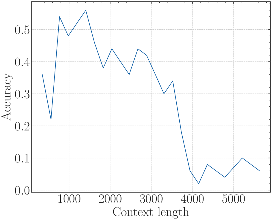
### Visual Description
# Technical Data Extraction: Accuracy vs. Context Length Chart
## 1. Component Isolation
* **Header:** None present.
* **Main Chart Area:** A 2D line plot featuring a single data series plotted against a grid.
* **Footer/Axes:** Contains the primary labels and numerical scales for the X and Y axes.
## 2. Axis and Label Extraction
* **Y-Axis Label:** `Accuracy` (Vertical orientation, left side).
* **Y-Axis Scale:** Numerical values ranging from `0.0` to `0.5` with major ticks every 0.1 units.
* **X-Axis Label:** `Context length` (Horizontal orientation, bottom center).
* **X-Axis Scale:** Numerical values ranging from `1000` to `5000` with major ticks every 1000 units. Minor ticks are visible between major intervals.
## 3. Data Series Analysis
* **Series Name:** Not explicitly labeled (Single series).
* **Color:** Dark Blue.
* **Visual Trend:**
* **Initial Volatility (0 - 1500):** The line starts at approximately 0.36, drops sharply to ~0.22, then climbs rapidly to its peak.
* **Peak Performance (1500):** Reaches its maximum value.
* **Gradual Decline (1500 - 3500):** The line exhibits a "sawtooth" downward trend, maintaining accuracy between 0.3 and 0.45.
* **Sharp Degradation (3500 - 4200):** A steep, near-linear drop in accuracy occurs.
* **Baseline/Noise (4200 - 5500+):** The accuracy flattens out at a very low level (below 0.1), showing minor fluctuations.
## 4. Data Point Extraction (Estimated)
Based on the grid intersections and axis markers, the following data points are extracted:
| Context Length (X) | Accuracy (Y) | Notes |
| :--- | :--- | :--- |
| ~400 | 0.36 | Starting point |
| ~600 | 0.22 | Local minimum |
| ~800 | 0.54 | Sharp recovery |
| 1000 | 0.48 | |
| ~1400 | 0.56 | **Global Maximum** |
| ~1600 | 0.46 | |
| ~1800 | 0.38 | |
| ~2100 | 0.44 | |
| ~2500 | 0.36 | |
| ~2700 | 0.44 | |
| ~2900 | 0.42 | |
| ~3300 | 0.30 | |
| ~3500 | 0.34 | Final peak before collapse |
| ~3900 | 0.06 | End of sharp decline |
| ~4200 | 0.02 | **Global Minimum** |
| ~4400 | 0.08 | |
| ~4800 | 0.04 | |
| ~5200 | 0.10 | |
| ~5600 | 0.06 | Final data point |
## 5. Summary of Findings
The chart illustrates a performance degradation of a system (likely a Large Language Model) as the input context length increases.
* **Optimal Range:** Context lengths between 800 and 1500 yield the highest accuracy (>0.5).
* **Stability Range:** Between 1500 and 3500, the system maintains a moderate accuracy (0.3 - 0.45).
* **Failure Point:** Beyond a context length of 3500, accuracy collapses significantly, suggesting the system reaches a functional limit or "context window" boundary, resulting in near-zero accuracy for lengths greater than 4000.
</details>
<details>
<summary>x20.png Details</summary>
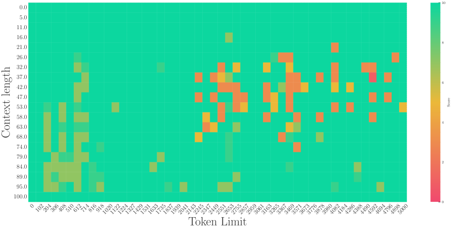
### Visual Description
# Technical Document Extraction: Performance Heatmap Analysis
## 1. Component Isolation
* **Header:** None present.
* **Main Chart Area:** A 2D heatmap representing "Score" across two variables: "Token Limit" (X-axis) and "Context length" (Y-axis).
* **Legend:** A vertical color bar located on the far right [x=right, y=center].
* **Axes:** Labeled X and Y axes with numerical markers.
---
## 2. Axis and Legend Extraction
### Y-Axis: Context length
* **Label:** Context length
* **Orientation:** Vertical (left side)
* **Scale:** 0.0 to 100.0
* **Markers:** 0.0, 5.0, 11.0, 16.0, 21.0, 26.0, 32.0, 37.0, 42.0, 47.0, 53.0, 58.0, 63.0, 68.0, 74.0, 79.0, 84.0, 89.0, 95.0, 100.0.
### X-Axis: Token Limit
* **Label:** Token Limit
* **Orientation:** Horizontal (bottom)
* **Scale:** 0 to 5000
* **Markers:** 0, 102, 204, 306, 408, 510, 612, 714, 816, 918, 1020, 1122, 1224, 1327, 1429, 1531, 1633, 1735, 1837, 1939, 2041, 2143, 2245, 2347, 2449, 2551, 2653, 2755, 2857, 2959, 3061, 3163, 3265, 3367, 3469, 3571, 3673, 3776, 3878, 3980, 4082, 4184, 4286, 4388, 4490, 4592, 4694, 4796, 4898, 5000.
### Legend: Score
* **Label:** Score
* **Type:** Continuous Gradient
* **Range:** 0 to 10
* **Color Mapping:**
* **10 (High):** Bright Teal/Green
* **5-7 (Medium):** Yellow/Orange
* **0 (Low):** Red/Pink
---
## 3. Trend Verification and Data Analysis
### Visual Trend Description
The heatmap is predominantly teal (Score 10), indicating high performance across most configurations. However, there are distinct "clusters of degradation" where the score drops into the 2–7 range (orange/yellow/red).
1. **Early Token Limit Cluster:** Between Token Limits 102 and 918, there is a vertical band of degradation across Context lengths 32.0 to 95.0.
2. **Mid-to-High Token Limit Cluster:** Between Token Limits 2143 and 4898, there is a scattered "cloud" of degradation, primarily concentrated between Context lengths 21.0 and 74.0.
3. **Stability Zone:** The top of the chart (Context length 0.0 to 16.0) and the far left (Token Limit 0) remain almost entirely teal (Score 10), regardless of other parameters.
### Key Data Points (Degradation Samples)
Based on the color-to-legend cross-referencing:
| Token Limit (X) | Context Length (Y) | Estimated Score | Color Note |
| :--- | :--- | :--- | :--- |
| 4490 | 37.0 | ~1-2 | Deep Pink/Red (Lowest observed) |
| 2551 | 37.0 | ~4-5 | Orange/Yellow |
| 612 | 32.0 | ~6-7 | Yellow-Green |
| 2653 | 16.0 | ~7 | Light Green/Yellow |
| 3469 | 74.0 | ~4 | Orange |
| 4898 | 26.0 | ~4 | Orange |
---
## 4. Summary of Information
This chart visualizes the performance (Score) of a system relative to its Token Limit and Context Length.
* **Optimal Performance:** Achieved at low Context lengths (<16.0) and very low Token Limits (<102).
* **Systemic Weakness:** The system shows significant performance drops (scores as low as 1-2) when the Token Limit is high (approx. 4500) and Context length is moderate (approx. 37.0).
* **Inconsistency:** There is a high degree of variance in the 2000-5000 Token Limit range, where scores fluctuate rapidly between 10 and 4 within small changes of Context length.
</details>
Figure 7: The first row: the results of a 2B model training from scratch with base=1e2. The second row: The results of fine-tuning the 2B model with base=1e4. The third row: The results of fine-tuning the 2B model with base=1e6.
According to and Theorem 1 and Eq. 18, this constraints could also apply to pre-training stage. To validate this, we trained a 2B model from scratch with RoPE base=100. The results, depicted in the first row of Figure 7, indicate that even though the model was trained with a context length of 4,096 tokens, it was capable of retrieving information from only the most recent approximately 500 tokens. This demonstrates that the base parameter bounds the context length during the pre-training stage as well. We define the context length from which the model can effectively retrieve information as the effective context length.
And according to our theory, the effective context length can be extended as the RoPE’s base increases. To validate this, we further fine-tune this 2B model on 32k context length, with RoPE’s base set to 1e4, as shown in the second row of Figure 7. While the effective context length increased, it remains significantly below 32k since the effective context length bounded by base=1e4 is much smaller than 32k. Further, when we increase the base to 1e6 and fine-tune the base 2B model on 32K (the third row in Figure 7), the model could obtain a larger context length than base=1e4, which is in accodance with our theory.
To further remove the influence of model size, we also fine-tuned a larger 7B model on a 32k context length with a RoPE base set to 1e4 and observed an effective context length nearly identical to that of the 2B model with the same RoPE base (see Appendix 14). This is empirical proof that the effective context length is determined by RoPE’s base.
5.4 Interpretation for the superficial long context capability for small base
Based on our theory and empirical observations, it is easy to explain what happens in Figure 3.
Better Extrapolation (Perplexity)? Due to the small base, $B_{m,\theta}$ can be smaller than zero as $m$ increases, which is shown in Figure 5. The model can’t attend more to similar tokens than random tokens with a large relative distance, so the model tends to focus more on nearby tokens, this will lead to a smaller empirical receptive field, even smaller than the training length. In this case, the model has a strong ability to maintain perplexity stability (Chi et al., 2023).
Worse Ability (Long-eval and NIH)! According to our previous analysis, RoPE’s base bounds the context length, and the context length bounded by 500 is much lower than that bound by 10,000. Therefore, when the base is set to 500, the effective context length drops sharply, even after training on 32k context length.
5.5 OOD theory is insufficient to reveal long context capability
Table 4: The comparison of "Method 1" and "Method 2". These methods are designed carefully. They both are no OOD, but they are very different under our theory.
| Method 1 | \usym 2718 | 0.33 | 0.27 | 0 | 0 |
| --- | --- | --- | --- | --- | --- |
| Method 2 | \usym 2718 | 0.40 | 0.00 | 97 | 2554 |
Section 3 mentions that methods based on the OOD theory of rotation angles may not fully reflect the long context capability. In this section, we conduct further experiments to substantiate and explain this observation. We present two methods to extend the context length of Llama2 from 4k to 32k. Both of them are devoid of OOD angles. These methods are delineated mathematically as follows:
- Method 1: $\theta_{i}=(5e6)^{-2i/d}$ ,
- Method 2: $\theta_{i}=\left\{\begin{aligned} &(1e4)^{-2i/128}/8,&i≥ 44\\
&(1e4*8^{128/88})^{-2i/128},&i<44.\end{aligned}\right.$
We can see from Table 4 that these two methods exhibit significantly different long context capabilities. Under the perspective of OOD rotation angle, both methods avoid OOD rotation angle, suggesting effective extrapolation. However, despite being trained on a context length of 32k, "method 2" struggles in completing the retrieval task at a context length of 32k. This phenomenon is beyond the scope which the OOD theory can explain.
Under our perspective, "method 2" is severely violating $B_{m,\theta}≥ 0$ when $m∈[15k,30k]$ , thereby impeding its ability to achieve long-context discrimination. We speculate that the model may achieve better extrapolation in the fine-tuning stage if the base is sufficiently large to surpass a lower bound and avoid OOD of rotation angles.
6 Related Work
Position embedding.
Since its introduction, Transformer (Vaswani et al., 2017) has achieved remarkable results in the field of natural language processing. To make full use of the order of sequence, researchers have introduced position embedding. The earliest position embedding was based on sinusoidal functions (Vaswani et al., 2017) for absolute positions, learnable absolute position embedding (Devlin et al., 2018) and many variants (Kiyono et al., 2021; Li et al., 2019) were proposed. Nevertheless, absolute position embedding has difficulties in extending directly to texts longer than the training length. Subsequently, researchers proposed relative position embedding methods (Shaw et al., 2018; Ke et al., 2020). With the development of large language models, rotary position embedding and its variants (Su et al., 2024; Sun et al., 2022) has become widely used, such as Llama2 (Touvron et al., 2023a), Baichuan2 (Yang et al., 2023), Mistral-7B- (Jiang et al., 2023a). A recent study reveals that no position embedding is also potential (Kazemnejad et al., 2024).
Long context learning.
Implementing models with longer or even infinitely long contexts has always been an important goal in the field of natural language processing. Due to the squared complexity of the transformer model over time, a significant portion of the work focuses on improving the model structure (Gu & Dao, 2023; 2023; Peng et al., 2023a; Qin et al., 2024). However, most of the work is still based on the transformer architecture. The other part of the work is aimed at reducing the computational complexity of attention itself, such as sparse attention (Beltagy et al., 2020) and group query attention (Ainslie et al., 2023). In addition, there are also some optimizations in engineering efficiency, such as flash attention (Dao et al., 2022) and ring attention (Liu et al., 2023). In the model inference stage, to save time and space, there are also some methods for accelerating long context, such as KV cache compression (Hooper et al., 2024), etc. And the position embedding is important in extrapolation. In the process of fine-tuning, methods such as PI (Chen et al., 2023), NTK, and YARN (Peng et al., 2023b) are used to change the original position embedding information. FoT (Tworkowski et al., 2024) assigns the position information of the tokens outside the local context as the first token in the local context.
7 Limitation
In this work, we investigate the relationship between the base of RoPE and context length. Although we have derived that there exists a lower bound for the base of RoPE determined by context length, the existence of the upper bound for RoPE’s base remains an open question that warrants further exploration. In addition, because of the lack of effective benchmarks for assessing long-context capabilities, the scope of long-context capabilities discussed in this paper may be limited.
8 Conclusion
Our work presents a comprehensive study on the role of RoPE in LLMs for effectively modeling long context. Our main contribution lies in uncovering a novel property of RoPE through theoretical analysis, demonstrating that as the relative distance between tokens increases, the model’s ability to attend more to similar tokens decreases. According to our theory, we derive a lower bound for RoPE’s base in accommodating to expected context lengths. Our experimental results validate that the base of RoPE bounds context length for not only fine-tuning but also the pre-training stage. Our theory offers a new perspective on understanding the functionality of RoPE in long-context modeling. By shedding light on the relationship between context length and position embedding, we hope our work could provide insights for enhancing the long context capability of LLMs.
References
- Achiam et al. (2023) Josh Achiam, Steven Adler, Sandhini Agarwal, Lama Ahmad, Ilge Akkaya, Florencia Leoni Aleman, Diogo Almeida, Janko Altenschmidt, Sam Altman, Shyamal Anadkat, et al. Gpt-4 technical report. arXiv preprint arXiv:2303.08774, 2023.
- Ainslie et al. (2023) Joshua Ainslie, James Lee-Thorp, Michiel de Jong, Yury Zemlyanskiy, Federico Lebron, and Sumit Sanghai. Gqa: Training generalized multi-query transformer models from multi-head checkpoints. In The 2023 Conference on Empirical Methods in Natural Language Processing, 2023.
- Bai et al. (2023) Jinze Bai, Shuai Bai, Yunfei Chu, Zeyu Cui, Kai Dang, Xiaodong Deng, Yang Fan, Wenbin Ge, Yu Han, Fei Huang, et al. Qwen technical report. arXiv preprint arXiv:2309.16609, 2023.
- Beltagy et al. (2020) Iz Beltagy, Matthew E Peters, and Arman Cohan. Longformer: The long-document transformer. arXiv preprint arXiv:2004.05150, 2020.
- bloc97 (2023) bloc97. Ntk-aware scaled rope allows llama models to have extended (8k+) context size without any fine-tuning and minimal perplexity degradation. https://www.reddit.com/r/LocalLLaMA/comments/14lz7j5/ntkaware_scaled_rope_allows_llama_models_to_have/, 2023.
- Chen et al. (2023) Shouyuan Chen, Sherman Wong, Liangjian Chen, and Yuandong Tian. Extending context window of large language models via positional interpolation. arXiv preprint arXiv:2306.15595, 2023.
- Chi et al. (2023) Ta-Chung Chi, Ting-Han Fan, Alexander Rudnicky, and Peter Ramadge. Dissecting transformer length extrapolation via the lens of receptive field analysis. In Proceedings of the 61st Annual Meeting of the Association for Computational Linguistics (Volume 1: Long Papers), pp. 13522–13537, 2023.
- Computer (2023) Together Computer. Redpajama: An open source recipe to reproduce llama training dataset, April 2023. URL https://github.com/togethercomputer/RedPajama-Data.
- Dao et al. (2022) Tri Dao, Dan Fu, Stefano Ermon, Atri Rudra, and Christopher Ré. Flashattention: Fast and memory-efficient exact attention with io-awareness. Advances in Neural Information Processing Systems, 35:16344–16359, 2022.
- Devlin et al. (2018) Jacob Devlin, Ming-Wei Chang, Kenton Lee, and Kristina Toutanova. Bert: Pre-training of deep bidirectional transformers for language understanding. arXiv preprint arXiv:1810.04805, 2018.
- emozilla (2023) emozilla. Dynamically scaled rope further increases performance of long context llama with zero fine-tuning. https://www.reddit.com/r/LocalLLaMA/comments/14mrgpr/dynamically_scaled_rope_further_increases/, 2023.
- G (2023) Kamradt G. Needle in a haystack - pressure testing llms. https://github.com/gkamradt/LLMTest_NeedleInAHaystack, 2023.
- Gu & Dao (2023) Albert Gu and Tri Dao. Mamba: Linear-time sequence modeling with selective state spaces. arXiv preprint arXiv:2312.00752, 2023.
- Han et al. (2023) Chi Han, Qifan Wang, Wenhan Xiong, Yu Chen, Heng Ji, and Sinong Wang. Lm-infinite: Simple on-the-fly length generalization for large language models. arXiv preprint arXiv:2308.16137, 2023.
- Heo et al. (2024) Byeongho Heo, Song Park, Dongyoon Han, and Sangdoo Yun. Rotary position embedding for vision transformer. arXiv preprint arXiv:2403.13298, 2024.
- Hooper et al. (2024) Coleman Hooper, Sehoon Kim, Hiva Mohammadzadeh, Michael W Mahoney, Yakun Sophia Shao, Kurt Keutzer, and Amir Gholami. Kvquant: Towards 10 million context length llm inference with kv cache quantization. arXiv preprint arXiv:2401.18079, 2024.
- Hu et al. (2024) Yutong Hu, Quzhe Huang, Mingxu Tao, Chen Zhang, and Yansong Feng. Can perplexity reflect large language model’s ability in long text understanding? In The Second Tiny Papers Track at ICLR 2024, 2024.
- Jiang et al. (2023a) Albert Q. Jiang, Alexandre Sablayrolles, Arthur Mensch, Chris Bamford, Devendra Singh Chaplot, Diego de las Casas, Florian Bressand, Gianna Lengyel, Guillaume Lample, Lucile Saulnier, Lélio Renard Lavaud, Marie-Anne Lachaux, Pierre Stock, Teven Le Scao, Thibaut Lavril, Thomas Wang, Timothée Lacroix, and William El Sayed. Mistral 7b, 2023a.
- Jiang et al. (2023b) Nan Jiang, Kevin Liu, Thibaud Lutellier, and Lin Tan. Impact of code language models on automated program repair. In 2023 IEEE/ACM 45th International Conference on Software Engineering (ICSE), pp. 1430–1442. IEEE, 2023b.
- Kazemnejad et al. (2024) Amirhossein Kazemnejad, Inkit Padhi, Karthikeyan Natesan Ramamurthy, Payel Das, and Siva Reddy. The impact of positional encoding on length generalization in transformers. Advances in Neural Information Processing Systems, 36, 2024.
- Ke et al. (2020) Guolin Ke, Di He, and Tie-Yan Liu. Rethinking positional encoding in language pre-training. In International Conference on Learning Representations, 2020.
- Kiyono et al. (2021) Shun Kiyono, Sosuke Kobayashi, Jun Suzuki, and Kentaro Inui. Shape: Shifted absolute position embedding for transformers. In Proceedings of the 2021 Conference on Empirical Methods in Natural Language Processing, pp. 3309–3321, 2021.
- Li* et al. (2023) Dacheng Li*, Rulin Shao*, Anze Xie, Ying Sheng, Lianmin Zheng, Joseph E. Gonzalez, Ion Stoica, Xuezhe Ma, and Hao Zhang. How long can open-source llms truly promise on context length?, June 2023. URL https://lmsys.org/blog/2023-06-29-longchat.
- Li et al. (2019) Hailiang Li, YC Adele, Yang Liu, Du Tang, Zhibin Lei, and Wenye Li. An augmented transformer architecture for natural language generation tasks. In 2019 International Conference on Data Mining Workshops (ICDMW), pp. 1–7. IEEE, 2019.
- Liu et al. (2023) Hao Liu, Matei Zaharia, and Pieter Abbeel. Ring attention with blockwise transformers for near-infinite context. In NeurIPS 2023 Foundation Models for Decision Making Workshop, 2023.
- Liu et al. (2024a) Hao Liu, Wilson Yan, Matei Zaharia, and Pieter Abbeel. World model on million-length video and language with ringattention. arXiv preprint arXiv:2402.08268, 2024a.
- Liu et al. (2024b) Xiaoran Liu, Hang Yan, Chenxin An, Xipeng Qiu, and Dahua Lin. Scaling laws of roPE-based extrapolation. In The Twelfth International Conference on Learning Representations, 2024b. URL https://openreview.net/forum?id=JO7k0SJ5V6.
- Mohtashami & Jaggi (2024) Amirkeivan Mohtashami and Martin Jaggi. Random-access infinite context length for transformers. Advances in Neural Information Processing Systems, 36, 2024.
- Peng et al. (2023a) Bo Peng, Eric Alcaide, Quentin Anthony, Alon Albalak, Samuel Arcadinho, Stella Biderman, Huanqi Cao, Xin Cheng, Michael Chung, Leon Derczynski, et al. Rwkv: Reinventing rnns for the transformer era. In Findings of the Association for Computational Linguistics: EMNLP 2023, pp. 14048–14077, 2023a.
- Peng et al. (2023b) Bowen Peng, Jeffrey Quesnelle, Honglu Fan, and Enrico Shippole. Yarn: Efficient context window extension of large language models. In The Twelfth International Conference on Learning Representations, 2023b.
- Qin et al. (2024) Zhen Qin, Songlin Yang, and Yiran Zhong. Hierarchically gated recurrent neural network for sequence modeling. Advances in Neural Information Processing Systems, 36, 2024.
- Rae et al. (2019) Jack W Rae, Anna Potapenko, Siddhant M Jayakumar, Chloe Hillier, and Timothy P Lillicrap. Compressive transformers for long-range sequence modelling. In International Conference on Learning Representations, 2019.
- Shaw et al. (2018) Peter Shaw, Jakob Uszkoreit, and Ashish Vaswani. Self-attention with relative position representations. In Proceedings of the 2018 Conference of the North American Chapter of the Association for Computational Linguistics: Human Language Technologies, Volume 2 (Short Papers), pp. 464–468, 2018.
- Shoeybi et al. (2020) Mohammad Shoeybi, Mostofa Patwary, Raul Puri, Patrick LeGresley, Jared Casper, and Bryan Catanzaro. Megatron-lm: Training multi-billion parameter language models using model parallelism, 2020.
- Su et al. (2024) Jianlin Su, Murtadha Ahmed, Yu Lu, Shengfeng Pan, Wen Bo, and Yunfeng Liu. Roformer: Enhanced transformer with rotary position embedding. Neurocomputing, 568:127063, 2024.
- Sun et al. (2022) Yutao Sun, Li Dong, Barun Patra, Shuming Ma, Shaohan Huang, Alon Benhaim, Vishrav Chaudhary, Xia Song, and Furu Wei. A length-extrapolatable transformer. arXiv preprint arXiv:2212.10554, 2022.
- Tay et al. (2022) Yi Tay, Mostafa Dehghani, Samira Abnar, Hyung Won Chung, William Fedus, Jinfeng Rao, Sharan Narang, Vinh Q Tran, Dani Yogatama, and Donald Metzler. Scaling laws vs model architectures: How does inductive bias influence scaling? arXiv preprint arXiv:2207.10551, 2022.
- Touvron et al. (2023a) Hugo Touvron, Thibaut Lavril, Gautier Izacard, Xavier Martinet, Marie-Anne Lachaux, Timothée Lacroix, Baptiste Rozière, Naman Goyal, Eric Hambro, Faisal Azhar, Aurelien Rodriguez, Armand Joulin, Edouard Grave, and Guillaume Lample. Llama: Open and efficient foundation language models, 2023a.
- Touvron et al. (2023b) Hugo Touvron, Louis Martin, Kevin Stone, Peter Albert, Amjad Almahairi, Yasmine Babaei, Nikolay Bashlykov, Soumya Batra, Prajjwal Bhargava, Shruti Bhosale, Dan Bikel, Lukas Blecher, Cristian Canton Ferrer, Moya Chen, Guillem Cucurull, David Esiobu, Jude Fernandes, Jeremy Fu, Wenyin Fu, Brian Fuller, Cynthia Gao, Vedanuj Goswami, Naman Goyal, Anthony Hartshorn, Saghar Hosseini, Rui Hou, Hakan Inan, Marcin Kardas, Viktor Kerkez, Madian Khabsa, Isabel Kloumann, Artem Korenev, Punit Singh Koura, Marie-Anne Lachaux, Thibaut Lavril, Jenya Lee, Diana Liskovich, Yinghai Lu, Yuning Mao, Xavier Martinet, Todor Mihaylov, Pushkar Mishra, Igor Molybog, Yixin Nie, Andrew Poulton, Jeremy Reizenstein, Rashi Rungta, Kalyan Saladi, Alan Schelten, Ruan Silva, Eric Michael Smith, Ranjan Subramanian, Xiaoqing Ellen Tan, Binh Tang, Ross Taylor, Adina Williams, Jian Xiang Kuan, Puxin Xu, Zheng Yan, Iliyan Zarov, Yuchen Zhang, Angela Fan, Melanie Kambadur, Sharan Narang, Aurelien Rodriguez, Robert Stojnic, Sergey Edunov, and Thomas Scialom. Llama 2: Open foundation and fine-tuned chat models, 2023b.
- Tworkowski et al. (2024) Szymon Tworkowski, Konrad Staniszewski, Mikołaj Pacek, Yuhuai Wu, Henryk Michalewski, and Piotr Miłoś. Focused transformer: Contrastive training for context scaling. Advances in Neural Information Processing Systems, 36, 2024.
- Vaswani et al. (2017) Ashish Vaswani, Noam Shazeer, Niki Parmar, Jakob Uszkoreit, Llion Jones, Aidan N Gomez, Łukasz Kaiser, and Illia Polosukhin. Attention is all you need. Advances in neural information processing systems, 30, 2017.
- Yang et al. (2023) Aiyuan Yang, Bin Xiao, Bingning Wang, Borong Zhang, Ce Bian, Chao Yin, Chenxu Lv, Da Pan, Dian Wang, Dong Yan, et al. Baichuan 2: Open large-scale language models. arXiv preprint arXiv:2309.10305, 2023.
- Young et al. (2024) Alex Young, Bei Chen, Chao Li, Chengen Huang, Ge Zhang, Guanwei Zhang, Heng Li, Jiangcheng Zhu, Jianqun Chen, Jing Chang, et al. Yi: Open foundation models by 01. ai. arXiv preprint arXiv:2403.04652, 2024.
Appendix A The proof of Theorem 1.
Assuming that the components of query $q∈ R^{d}$ and key $k∈ R^{d}$ are independent, their standard deviations are denoted as $\sigma∈ R^{d}$ and the means are donated as $\mu∈ R^{d}$ . The key $k^{*}$ similar to $q$ is $q+\epsilon$ , where $\epsilon$ is a random variable with a mean of 0. Then, we have:
$$
\displaystyle\mathbb{E}_{q,k^{*}}q^{T}R_{m}k^{*}-\mathbb{E}_{q,k}q^{T}R_{m}k \displaystyle= \displaystyle\mathbb{E}_{q}q^{T}R_{m}q+\mathbb{E}_{q,\epsilon}q^{T}R_{m}\epsilon-\mathbb{E}_{q,k}q^{T}R_{m}k \displaystyle= \displaystyle\mathbb{E}_{q}\sum_{i=0}^{d/2-1}(q_{2i}^{2}\cos(m\theta_{i})-q_{2i}q_{2i+1}sin(m\theta_{i})+q_{2i+1}q_{2i}sin(m\theta_{i})+q_{2i+1}^{2}\cos(m\theta_{i}))+\mathbb{E}_{q}q^{T}R_{m}\mathbb{E}_{\epsilon}\epsilon \displaystyle-\mathbb{E}_{q,k}\sum_{i=0}^{d/2-1}(q_{2i}k_{2i}\cos(m\theta_{i})-q_{2i}k_{2i+1}sin(m\theta_{i})+q_{2i+1}k_{2i}sin(m\theta_{i})+q_{2i+1}k_{2i+1}\cos(m\theta_{i})) \displaystyle= \displaystyle\sum_{i=0}^{d/2-1}\mathbb{E}(q_{2i}^{2})\cos(m\theta_{i})-\mu_{2i}\mu_{2i+1}sin(m\theta_{i})+\mu_{2i}\mu_{2i+1}sin(m\theta_{i})+\mathbb{E}(q_{2i+1}^{2})\cos(m\theta_{i}))+\mu R_{m}0 \displaystyle-\sum_{i=0}^{d/2-1}(\mu_{2i}^{2}\cos(m\theta_{i})-\mu_{2i}\mu_{2i+1}sin(m\theta_{i})+\mu_{i}\mu_{2i+1}sin(m\theta_{i})+\mu_{2i+1}^{2}\cos(m\theta_{i})) \displaystyle= \displaystyle\sum_{i=0}^{d/2-1}(E(q_{2i}^{2}+q_{2i+1}^{2})-\mu_{2i}^{2}-\mu_{2i+1}^{2})\cos(m\theta_{i}) \displaystyle= \displaystyle\sum_{i=0}^{d/2-1}(\sigma_{i}^{2}+\sigma_{i+1}^{2})\cos(m\theta_{i}) \tag{19}
$$
Then we can get:
$$
\displaystyle\sum_{i=0}^{d/2-1}(\sigma_{2i}^{2}+\sigma_{2i+1}^{2})\cos(m\theta_{i})=\mathbb{E}_{q,k^{*}}q^{T}R_{m}k^{*}-\mathbb{E}_{q,k}q^{T}R_{m}k \tag{20}
$$
And when all $\sigma$ are equal, we can get:
$$
\displaystyle\sum_{i=0}^{d/2-1}\cos(m\theta_{i})=\frac{1}{2\sigma^{2}}(\mathbb{E}_{q,k^{*}}q^{T}R_{m}k^{*}-\mathbb{E}_{q,k}q^{T}R_{m}k) \tag{21}
$$
Appendix B The detail setting of experiment.
For training, we mainly conducted experiments on Llama2-7B (Touvron et al., 2023a) and Baichuan2-7B (Yang et al., 2023). In addition, we also trained a 2B model from scratch, whose structure is the same with Baichuan2-7B-Base but with a smaller hidden size = 2048. Both training and testing are accelerated by FlashAttention-2 (Dao et al., 2022) and Megatron-LM (Shoeybi et al., 2020). The dataset of both fine-tuning and training from scratch is a subset of RedPajama (Computer, 2023). The hyper parameters of training are list in Appendix 5. All experiments are conducted on a cluster of 16 machines with 128 NVIDIA A100 80G.
Table 5: Training hyper-parameters in our experiments
| Llama2-7B-Base | 32K | 4B | 128 | 2e5 | constant | 0 |
| --- | --- | --- | --- | --- | --- | --- |
| Baichuan2-7B-Base | 32K | 4B | 128 | 2e5 | constant | 0 |
| Our-2B-Base | 4K | 1T | 1024 | 2e4 | cosine | 0.1 |
For evaluation, we test the long context capabilities comprehensively, the benchmarks are listed below: perplexity on PG19 (Rae et al., 2019) test split. We evaluate the perplexity of each sample and get the mean value across samples.
Long-eval (Li* et al., 2023). This test generates massive random similar sentences and asks the model to answer questions according to a specific sentence in the context. Because the long context consists of many similar patterns, it’s more difficult to get the right answer. We find this test is harder than other long context evaluations such as Perplexity, Passkey Retrieval (Mohtashami & Jaggi, 2024), Needle in Haystack (G, 2023). A test sample is list in Figure 8
<details>
<summary>x21.png Details</summary>
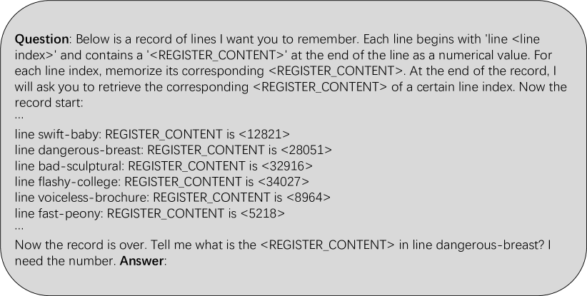
### Visual Description
### Technical Document Extraction: Text-Based Instruction Record
**Image Overview:**
The image contains a block of text formatted as a prompt or a logic test. It is presented on a light gray background with rounded corners and a thin black border. The text is written in English and follows a structured pattern designed to test memory or data retrieval capabilities.
---
#### 1. Component Isolation
* **Header/Instruction Block:** Defines the task and the format of the data.
* **Data Record Block:** A list of specific identifiers (line indices) and their associated numerical values (register contents).
* **Footer/Query Block:** Concludes the record and asks a specific question based on the provided data.
---
#### 2. Text Transcription
**Instruction Block:**
> **Question:** Below is a record of lines I want you to remember. Each line begins with 'line <line index>' and contains a '<REGISTER_CONTENT>' at the end of the line as a numerical value. For each line index, memorize its corresponding <REGISTER_CONTENT>. At the end of the record, I will ask you to retrieve the corresponding <REGISTER_CONTENT> of a certain line index. Now the record start:
> ...
**Data Record Block:**
| Line Index | REGISTER_CONTENT |
| :--- | :--- |
| swift-baby | 12821 |
| dangerous-breast | 28051 |
| bad-sculptural | 32916 |
| flashy-college | 34027 |
| voiceless-brochure | 8964 |
| fast-peony | 5218 |
*Note: The ellipsis (...) indicates that this is a snippet of a potentially larger record.*
**Query Block:**
> ...
> Now the record is over. Tell me what is the <REGISTER_CONTENT> in line dangerous-breast? I need the number. **Answer:**
---
#### 3. Data Analysis and Facts
* **Format:** The data follows a strict syntax: `line [string-identifier]: REGISTER_CONTENT is <[integer]>`.
* **Target Information:** The query specifically requests the value associated with the index **"dangerous-breast"**.
* **Extracted Value:** Based on the second entry in the data record block, the value for "dangerous-breast" is **28051**.
* **Language:** The text is entirely in English. No other languages are present.
---
#### 4. Summary of Information
The image serves as a "needle-in-a-haystack" style memory test. It provides six unique alphanumeric keys paired with five-digit (and one four-digit) integers. The document concludes by asking for the retrieval of the second item in the list.
</details>
Figure 8: Long-eval sample prompt
needle in haystack(NIH) (G, 2023). NIH tests the long context capability not only under different context lengths but also at different positions where the correct answer is located in the context, which provides a more detailed view of the long context capability.
Appendix C Baichuan2-7B-Base: Lower bound Base of RoPE
<details>
<summary>x22.png Details</summary>
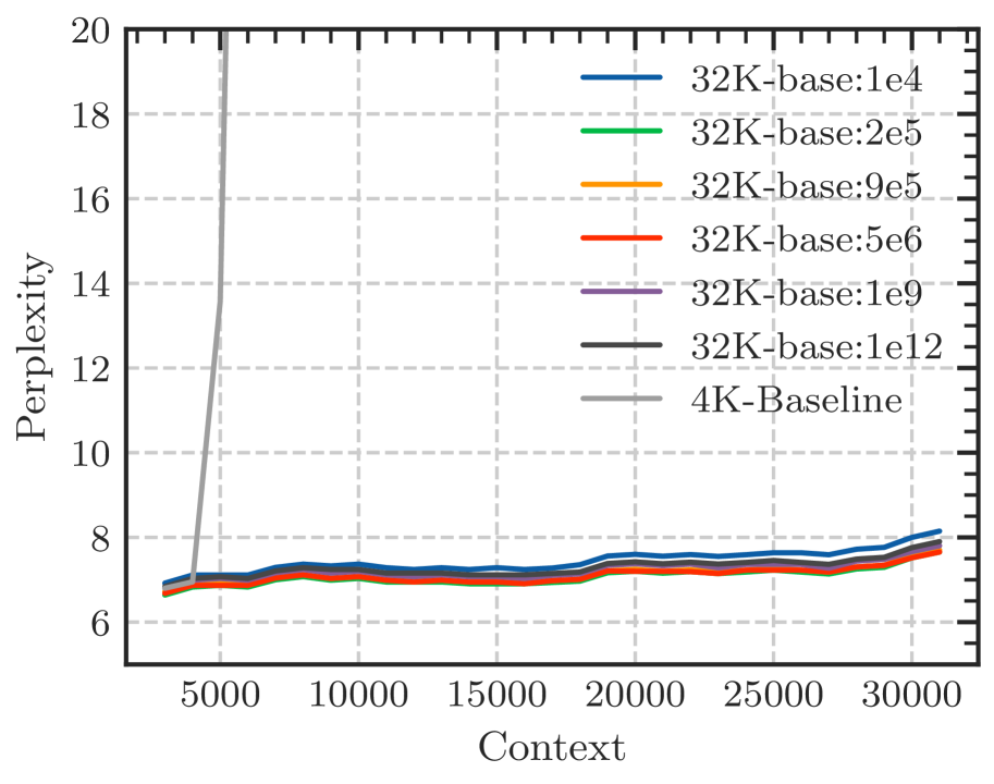
### Visual Description
# Technical Document Extraction: Perplexity vs. Context Length Chart
## 1. Component Isolation
* **Header:** None.
* **Main Chart Area:** A line graph plotting "Perplexity" (Y-axis) against "Context" (X-axis). It features a grid of dashed light-gray lines.
* **Legend:** Located in the upper-right quadrant of the chart area.
* **Axes:**
* **Y-axis (Vertical):** Labeled "Perplexity", ranging from 6 to 20 with major increments of 2.
* **X-axis (Horizontal):** Labeled "Context", ranging from approximately 4,000 to 32,000 with major labeled increments every 5,000 units (5000, 10000, 15000, 20000, 25000, 30000).
## 2. Legend Data Extraction
The legend is positioned at approximately `[x=0.75, y=0.25]` relative to the top-left corner of the image.
| Color | Label | Description |
| :--- | :--- | :--- |
| Blue | `32K-base:1e4` | 32K base model with 1e4 parameter/setting |
| Green | `32K-base:2e5` | 32K base model with 2e5 parameter/setting |
| Orange | `32K-base:9e5` | 32K base model with 9e5 parameter/setting |
| Red | `32K-base:5e6` | 32K base model with 5e6 parameter/setting |
| Purple | `32K-base:1e9` | 32K base model with 1e9 parameter/setting |
| Dark Gray | `32K-base:1e12` | 32K base model with 1e12 parameter/setting |
| Light Gray | `4K-Baseline` | Baseline model with 4K context limit |
## 3. Trend Verification and Data Analysis
### Series 1: 4K-Baseline (Light Gray)
* **Trend:** This line starts at a perplexity of ~7 at context 4,000. Immediately after the 4,000 mark, the line slopes sharply upward (vertically), exceeding the Y-axis limit of 20 before reaching context 6,000.
* **Significance:** Indicates total model failure/catastrophic perplexity increase once the context exceeds its trained limit of 4,000.
### Series 2-7: 32K-base variants (Multi-colored)
* **Trend:** All six "32K-base" lines follow a nearly identical, stable horizontal trajectory. They start between perplexity 6.5 and 7.0 at context 4,000 and remain below 8.5 even as context reaches 32,000. There is a very slight, gradual upward drift as context increases.
* **Relative Performance (Stacking Order):**
* **Highest Perplexity (Worst):** Blue (`32K-base:1e4`) consistently sits at the top of the cluster.
* **Lowest Perplexity (Best):** Red (`32K-base:5e6`) consistently sits at the bottom of the cluster.
* **Middle Cluster:** The Green, Orange, Purple, and Dark Gray lines are tightly interleaved between the Blue and Red lines, showing marginal differences in performance.
## 4. Key Data Points (Approximate)
| Context | 4K-Baseline (Perplexity) | 32K-base Cluster (Perplexity Range) |
| :--- | :--- | :--- |
| 4,000 | ~7.0 | 6.8 - 7.1 |
| 5,000 | ~14.0 (Rising sharply) | 6.9 - 7.2 |
| 10,000 | > 20 (Off-chart) | 7.0 - 7.4 |
| 20,000 | > 20 (Off-chart) | 7.2 - 7.6 |
| 30,000 | > 20 (Off-chart) | 7.5 - 8.0 |
| 32,000 | > 20 (Off-chart) | 7.8 - 8.2 |
## 5. Summary of Findings
The chart demonstrates the effectiveness of the "32K-base" model variants in maintaining low perplexity (high performance) across long context windows up to 32,000 tokens. In contrast, the "4K-Baseline" model experiences an immediate and extreme loss of performance as soon as the context window exceeds its 4,000-token design limit. Among the 32K variants, the `5e6` (Red) configuration appears to provide the most stable and lowest perplexity.
</details>
(a) Perplexity
<details>
<summary>x23.png Details</summary>
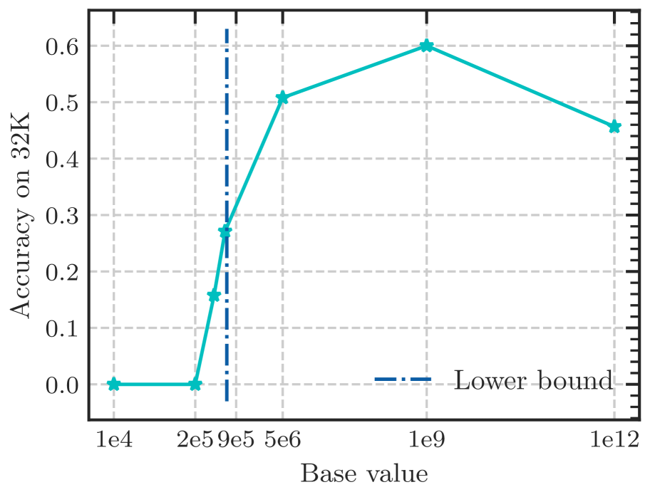
### Visual Description
# Technical Document Extraction: Accuracy vs. Base Value Chart
## 1. Component Isolation
* **Header:** None present.
* **Main Chart Area:** A line graph with a logarithmic-style x-axis and a linear y-axis. It features a single data series (teal line with star markers) and a vertical reference line (dark blue dash-dotted line).
* **Legend:** Located in the bottom-right quadrant of the plot area.
* **Footer/Axes:** X-axis labeled "Base value" and Y-axis labeled "Accuracy on 32K".
---
## 2. Axis and Metadata Extraction
* **Y-Axis (Vertical):**
* **Label:** Accuracy on 32K
* **Scale:** Linear, ranging from 0.0 to 0.6.
* **Major Tick Marks:** 0.0, 0.1, 0.2, 0.3, 0.4, 0.5, 0.6.
* **X-Axis (Horizontal):**
* **Label:** Base value
* **Scale:** Non-linear/Logarithmic-style spacing.
* **Major Tick Labels:** 1e4, 2e5, 9e5, 5e6, 1e9, 1e12.
* **Grid:** Light gray dashed horizontal and vertical grid lines corresponding to major ticks.
* **Legend [Spatial Grounding: Bottom Right]:**
* **Label:** "Lower bound"
* **Style:** Dark blue dash-dotted line (`- . - .`).
---
## 3. Data Series Analysis
### Series 1: Accuracy Data
* **Color:** Teal / Cyan.
* **Marker:** 5-point star.
* **Trend Verification:** The line starts at zero for low base values, exhibits a sharp upward slope between $2 \times 10^5$ and $1 \times 10^9$, reaches a peak at $1 \times 10^9$, and then shows a slight downward slope toward $1 \times 10^{12}$.
| Base value (X) | Accuracy on 32K (Y) | Notes |
| :--- | :--- | :--- |
| 1e4 | 0.0 | Baseline zero |
| 2e5 | 0.0 | Remains at zero |
| ~5e5* | ~0.16 | Intermediate point (unlabeled x-tick) |
| 9e5 | ~0.27 | Sharp increase |
| 5e6 | ~0.51 | Continued sharp increase |
| 1e9 | 0.6 | **Peak Accuracy** |
| 1e12 | ~0.46 | Performance degradation |
*\*Note: There is a data point between 2e5 and 9e5 that is not explicitly labeled on the x-axis but aligns with the vertical grid line.*
### Reference Element: Lower Bound
* **Color:** Dark Blue.
* **Style:** Vertical dash-dotted line.
* **Placement:** Positioned at the x-axis value of **9e5**.
* **Intersection:** This line intersects the teal data series at an accuracy of approximately 0.27.
---
## 4. Summary of Findings
This chart illustrates the relationship between a "Base value" and the "Accuracy on 32K".
1. **Inertia Phase:** For base values at or below $2 \times 10^5$, the accuracy is effectively 0.0.
2. **Growth Phase:** A rapid improvement in accuracy occurs as the base value increases from $2 \times 10^5$ to $1 \times 10^9$.
3. **Critical Threshold:** The "Lower bound" is marked at $9 \times 10^5$, which represents the point where accuracy has climbed to roughly 27%.
4. **Optimal Point:** Maximum accuracy (0.6) is achieved when the base value is $1 \times 10^9$.
5. **Saturation/Regression:** Increasing the base value further to $1 \times 10^{12}$ results in a decrease in accuracy to approximately 0.46, suggesting an over-optimization or diminishing returns beyond the $10^9$ threshold.
</details>
(b) Long-eval 32k
Figure 9: Fine-tuning Baichuan2-7B-Base on 32k context length with varying RoPE’s base. Although the perplexity remains low with varying bases, the Long-eval accuracy revels a discernible bound for the base value, below which the Long-eval accuracy declines significantly. the dotted line denotes the lower bound derived from Eq. 18.
Appendix D Long Context Test Results on Various LLMs
<details>
<summary>x24.png Details</summary>
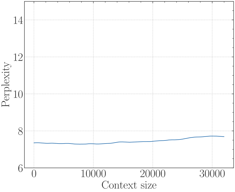
### Visual Description
# Technical Document Extraction: Perplexity vs. Context Size Chart
## 1. Image Overview
This image is a line graph illustrating the relationship between "Perplexity" and "Context size" for a computational model (likely a Large Language Model). The chart uses a clean, academic style with a serif font and a light gray grid.
## 2. Component Isolation
### Header/Title
* **Content:** None present.
### Main Chart Area
* **Background:** White with a light gray dashed grid.
* **Grid Lines:** Vertical grid lines occur every 10,000 units on the x-axis. Horizontal grid lines occur every 2 units on the y-axis.
* **Data Series:** A single solid dark blue line.
### Axis Labels and Markers
* **Y-Axis (Vertical):**
* **Label:** "Perplexity" (oriented vertically).
* **Scale:** 6 to 15 (visible range).
* **Major Tick Marks:** 6, 8, 10, 12, 14.
* **Minor Tick Marks:** Present between major ticks, indicating increments of 1 unit.
* **X-Axis (Horizontal):**
* **Label:** "Context size".
* **Scale:** 0 to approximately 32,000.
* **Major Tick Marks:** 0, 10000, 20000, 30000.
* **Minor Tick Marks:** Present at intervals of 2,500 units.
### Legend
* **Location:** Not present. As there is only one data series, the blue line represents the primary metric.
## 3. Data Extraction and Trend Analysis
### Trend Verification
* **Series 1 (Dark Blue Line):** The line begins at a context size of 0 with a perplexity value slightly above 7. It remains remarkably stable and flat for the first 15,000 units, showing a very slight downward dip before recovering. After the 15,000 mark, the line exhibits a very gradual upward slope, ending just below the 8.0 mark at a context size of 32,000.
### Estimated Data Points
Based on the grid alignment, the following values are extracted:
| Context size (x) | Perplexity (y) | Notes |
| :--- | :--- | :--- |
| 0 | ~7.3 | Starting point. |
| 5,000 | ~7.3 | Stable. |
| 10,000 | ~7.2 | Slightest local minimum. |
| 15,000 | ~7.4 | Beginning of very gradual ascent. |
| 20,000 | ~7.5 | Continuing gradual ascent. |
| 25,000 | ~7.6 | Continuing gradual ascent. |
| 30,000 | ~7.7 | Near peak of the visible range. |
| 32,000 | ~7.7 | Final data point; slight plateau/dip at the very end. |
## 4. Technical Summary
The chart demonstrates the **stability of model performance** (measured by perplexity) as the input context window increases.
* **Key Finding:** The perplexity remains within a very narrow band (approximately 7.2 to 7.7) across a context size of 0 to 32,000 tokens.
* **Significance:** In language modeling, lower perplexity indicates better performance. The fact that the line does not "explode" or rise sharply at higher context sizes suggests the model maintains its predictive accuracy and coherence even when processing very long sequences of text.
</details>
<details>
<summary>x25.png Details</summary>
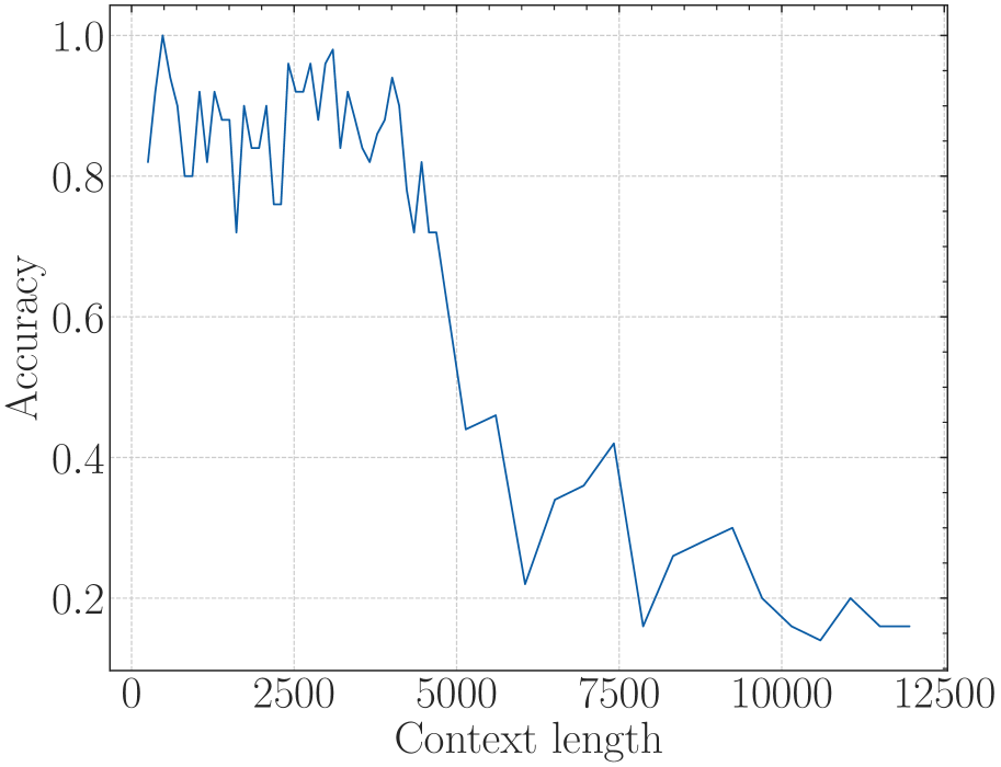
### Visual Description
# Technical Document Extraction: Performance Analysis Chart
## 1. Component Isolation
* **Header:** None present.
* **Main Chart Area:** A line graph plotted on a Cartesian coordinate system with a light-gray dashed grid.
* **Footer/Axes:** Contains the X-axis label "Context length" and the Y-axis label "Accuracy".
## 2. Axis and Label Extraction
* **Y-Axis Label:** Accuracy (Vertical orientation, left side).
* **Y-Axis Markers:** 0.2, 0.4, 0.6, 0.8, 1.0.
* **X-Axis Label:** Context length (Horizontal orientation, bottom center).
* **X-Axis Markers:** 0, 2500, 5000, 7500, 10000, 12500.
* **Legend:** No legend is present as there is only a single data series.
## 3. Data Series Analysis
* **Series Color:** Dark Blue.
* **Visual Trend:**
* **Phase 1 (0 to ~4500):** High volatility but generally high performance. The line oscillates frequently between 0.7 and 1.0.
* **Phase 2 (~4500 to ~5500):** Sharp downward slope. A significant "cliff" where performance drops precipitously.
* **Phase 3 (~5500 to 12500):** Low-performance regime. The line continues to fluctuate but stays primarily between 0.15 and 0.45, showing a gradual overall decline toward the end of the range.
## 4. Key Data Points (Estimated from Visual Mapping)
| Context Length (X) | Accuracy (Y) | Note |
| :--- | :--- | :--- |
| ~250 | ~0.82 | Starting point |
| ~500 | 1.0 | Peak performance |
| ~1500 | ~0.72 | Local minimum in high-perf zone |
| ~3200 | ~0.98 | Late-stage peak |
| ~4500 | ~0.82 | Start of the major decline |
| ~5200 | ~0.44 | End of initial sharp drop |
| ~6000 | ~0.22 | Local minimum |
| ~7400 | ~0.42 | Local recovery peak |
| ~7800 | ~0.16 | Significant low point |
| ~9200 | ~0.30 | Small recovery |
| ~10500 | ~0.14 | Absolute minimum |
| ~12000 | ~0.16 | Final data point |
## 5. Summary of Findings
The chart illustrates a "performance cliff" characteristic of many Large Language Models (LLMs) or retrieval systems. The system maintains high accuracy (averaging ~0.85) for context lengths up to approximately 4,500 units. Beyond this threshold, there is a catastrophic failure in accuracy, which drops below 0.5 and never recovers to its previous levels, eventually bottoming out near 0.15 as the context length approaches 12,500.
</details>
<details>
<summary>x26.png Details</summary>
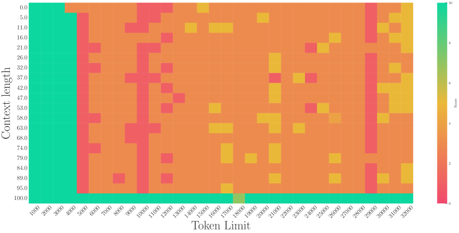
### Visual Description
# Technical Document Extraction: Performance Heatmap Analysis
## 1. Document Overview
This image is a technical heatmap visualizing the relationship between **Context length** and **Token Limit** relative to a performance **Score**. The chart uses a color gradient to represent numerical values, typically used in Large Language Model (LLM) "Needle In A Haystack" or context window evaluations.
## 2. Component Isolation
### A. Header / Metadata
* **Language:** English.
* **Primary Axis Labels:** "Context length" (Y-axis) and "Token Limit" (X-axis).
### B. Main Chart (Heatmap Grid)
* **X-Axis (Token Limit):** Represents numerical values ranging from 1,000 to 32,000.
* **Markers:** 1000, 2000, 3000, 4000, 5000, 6000, 7000, 8000, 9000, 10000, 11000, 12000, 13000, 14000, 15000, 16000, 17000, 18000, 19000, 20000, 21000, 22000, 23000, 24000, 25000, 26000, 27000, 28000, 29000, 30000, 31000, 32000.
* **Y-Axis (Context length):** Represents percentage-based or indexed values from 0.0 to 100.0.
* **Markers:** 0.0, 5.0, 11.0, 16.0, 21.0, 26.0, 32.0, 37.0, 42.0, 47.0, 53.0, 58.0, 63.0, 68.0, 74.0, 79.0, 84.0, 89.0, 95.0, 100.0.
### C. Legend (Color Scale)
* **Location:** Right side of the chart.
* **Label:** "Score"
* **Scale:** 0 to 10.
* **Color Mapping:**
* **Bright Green (Value 10):** Perfect/High performance.
* **Yellow/Gold (Value ~5-6):** Moderate performance.
* **Orange (Value ~3-4):** Low performance.
* **Pink/Red (Value 0-2):** Failure/Very low performance.
---
## 3. Trend Verification and Data Extraction
### Visual Trend Analysis
1. **High Performance Zone (Green):** There is a distinct vertical band of green on the far left (Token Limits 1,000 to 4,000) across almost all context lengths. There is also a horizontal band of green at the very bottom (Context length 100.0) across almost all token limits.
2. **Degradation Zone (Orange/Red):** As the Token Limit increases beyond 4,000, the performance drops sharply into the orange (score ~3) and pink (score ~1) range.
3. **Inconsistency:** The central area of the map is predominantly orange, interspersed with "noise" or specific failure points (pink) and occasional moderate successes (yellow).
### Key Data Observations
| Region | Token Limit Range | Context Length Range | Dominant Color | Estimated Score |
| :--- | :--- | :--- | :--- | :--- |
| **Initial Success** | 1,000 - 4,000 | 0.0 - 100.0 | Green | 10 |
| **Base Success** | 1,000 - 32,000 | 100.0 | Green | 10 |
| **General Failure** | 5,000 - 32,000 | 0.0 - 95.0 | Orange/Pink | 1 - 4 |
### Specific Anomalies (Yellow/Gold "Moderate" Points)
Occasional yellow blocks (Score ~5-7) appear sporadically in the "failure" zone, notably at:
* **Token Limit 16,000 - 17,000:** Scattered yellow blocks across various context lengths.
* **Token Limit 21,000:** A vertical cluster of yellow blocks between context lengths 26.0 and 53.0.
* **Token Limit 31,000 - 32,000:** Several yellow blocks at the upper context lengths.
### Specific Failures (Pink "Low" Points)
Vertical bands of pink (Score ~0-1) are visible, suggesting systematic failure at specific token limits regardless of context length:
* **Token Limit 5,000:** Almost entirely pink/red.
* **Token Limit 10,000:** Almost entirely pink/red.
* **Token Limit 29,000:** Almost entirely pink/red.
---
## 4. Summary of Findings
The data indicates a model that performs perfectly at very low token limits (under 4,000) or when the "needle" is at the very end of the context (100.0 length). However, for the vast majority of the tested space (Token limits > 4,000 and context positions < 100.0), the model exhibits significant performance degradation, with specific "dead zones" occurring at intervals of 5,000, 10,000, and 29,000 tokens.
</details>
Figure 10: Llama2-7B-Base with base=1e4 fine-tuned on 32k context (original context=4096)
<details>
<summary>x27.png Details</summary>

### Visual Description
# Technical Document Extraction: Perplexity vs. Context Size Chart
## 1. Image Overview
This image is a line graph illustrating the relationship between "Perplexity" and "Context size" for a computational model (likely a Large Language Model). The chart uses a clean, academic style with a serif font and a light gray grid.
## 2. Component Isolation
### Header/Title
* **Content:** None present.
### Main Chart Area
* **Type:** Line Graph.
* **Background:** White with a light gray dashed grid.
* **Grid Lines:** Vertical grid lines occur every 10,000 units on the x-axis. Horizontal grid lines occur every 2 units on the y-axis.
### Axis Labels and Markers
* **Y-Axis (Vertical):**
* **Label:** "Perplexity" (oriented vertically).
* **Scale:** 6 to 14.
* **Major Tick Marks:** 6, 8, 10, 12, 14.
* **Minor Tick Marks:** Present between major intervals (representing increments of 1).
* **X-Axis (Horizontal):**
* **Label:** "Context size".
* **Scale:** 0 to 30,000+.
* **Major Tick Marks:** 0, 10000, 20000, 30000.
* **Minor Tick Marks:** Present at intervals of 2,500 units.
### Legend
* **Location:** Not present. There is only a single data series.
---
## 3. Data Series Analysis
### Series 1: Perplexity Performance
* **Color:** Dark Blue.
* **Trend Verification:** The line begins at a low perplexity value and remains remarkably stable. It exhibits a very slight downward dip in the first third of the graph, followed by a very gradual upward slope as the context size increases toward 32,000. The overall trend is "near-horizontal stability," indicating the model maintains consistent performance across varying context lengths.
### Estimated Data Points
Based on the grid alignment:
| Context Size (x) | Perplexity (y) | Notes |
| :--- | :--- | :--- |
| 0 | ~7.4 | Starting point. |
| 5,000 | ~7.3 | Slight decrease/dip. |
| 10,000 | ~7.3 | Local minimum. |
| 15,000 | ~7.4 | Returning to baseline. |
| 20,000 | ~7.5 | Very gradual increase. |
| 25,000 | ~7.6 | Continued gradual increase. |
| 30,000 | ~7.7 | Peak perplexity in this range. |
| 32,000 | ~7.7 | Final data point, slight plateau. |
---
## 4. Technical Summary
The chart demonstrates the model's ability to handle long-range dependencies. In many language models, perplexity (a measure of uncertainty) tends to spike or degrade significantly as context size increases. This specific data shows a highly robust model where perplexity remains within a very narrow band (approximately 7.3 to 7.7) even as the context size scales from 0 to over 30,000 tokens. This suggests effective architectural scaling or the use of techniques like RoPE (Rotary Positional Embeddings) or Alibi that mitigate performance loss at high context lengths.
</details>
<details>
<summary>x28.png Details</summary>
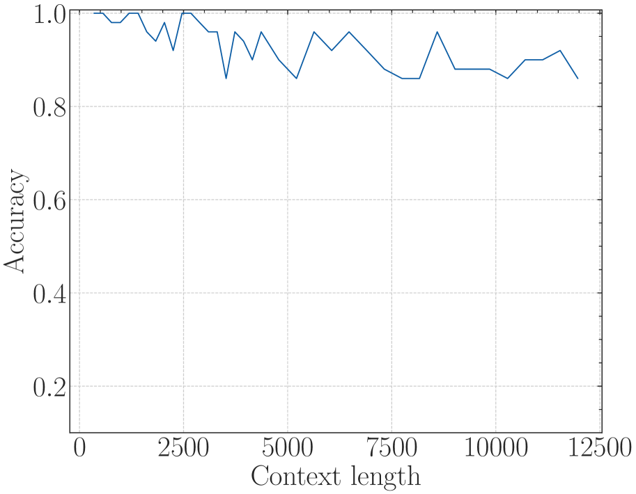
### Visual Description
# Technical Document Extraction: Accuracy vs. Context Length Chart
## 1. Image Classification and Overview
This image is a line chart depicting the relationship between model performance (Accuracy) and the length of input data (Context length). The chart uses a serif font, typical of LaTeX-rendered academic documents.
## 2. Component Isolation
### A. Header/Title
* **Content:** None present.
### B. Main Chart Area (Data Visualization)
* **Type:** 2D Line Plot.
* **Grid:** Light gray dashed grid lines are present for both major x and y intervals.
* **Data Series:** A single solid dark blue line.
* **Background:** White.
### C. Axes and Labels
* **Y-Axis (Vertical):**
* **Label:** "Accuracy" (oriented vertically).
* **Scale:** Linear, ranging from 0.1 to 1.0.
* **Major Tick Markers:** 0.2, 0.4, 0.6, 0.8, 1.0.
* **X-Axis (Horizontal):**
* **Label:** "Context length" (oriented horizontally).
* **Scale:** Linear, ranging from 0 to 12,500.
* **Major Tick Markers:** 0, 2500, 5000, 7500, 10000, 12500.
### D. Legend
* **Content:** None present. The chart contains only one data series.
---
## 3. Data Extraction and Trend Analysis
### Trend Verification
The blue line represents the accuracy of a system as context length increases.
* **Initial Phase (0 - 2,500):** The line starts at a perfect 1.0 accuracy. It exhibits high-frequency volatility but remains generally high (above 0.9).
* **Middle Phase (2,500 - 7,500):** The line shows a gradual downward trend with significant "sawtooth" fluctuations. It drops to its local minimum near the 3,500 mark before recovering and then slowly declining toward 0.85.
* **Final Phase (7,500 - 12,500):** The accuracy stabilizes in a lower band, fluctuating primarily between 0.85 and 0.95, ending with a slight downward tick at the 12,000+ mark.
### Estimated Data Points
*Note: Values are estimated based on pixel alignment with the grid.*
| Context Length (Approx.) | Accuracy (Approx.) |
| :--- | :--- |
| 500 | 1.00 |
| 1,000 | 0.98 |
| 1,500 | 1.00 |
| 2,000 | 0.95 |
| 2,500 | 1.00 |
| 3,500 | 0.86 (Local Minimum) |
| 4,500 | 0.96 |
| 5,500 | 0.86 |
| 6,000 | 0.96 |
| 8,000 | 0.86 |
| 9,000 | 0.96 |
| 10,000 | 0.88 |
| 11,500 | 0.92 |
| 12,000 | 0.86 |
---
## 4. Technical Summary
The chart demonstrates that the model maintains high accuracy (above 85%) across the tested context window of 12,500 units. However, there is a clear inverse correlation: as the **Context length** increases, the **Accuracy** becomes more volatile and shows a slight overall degradation from a perfect 1.0 to a range centered around 0.9. The most stable performance is observed at context lengths under 2,500.
</details>
<details>
<summary>x29.png Details</summary>
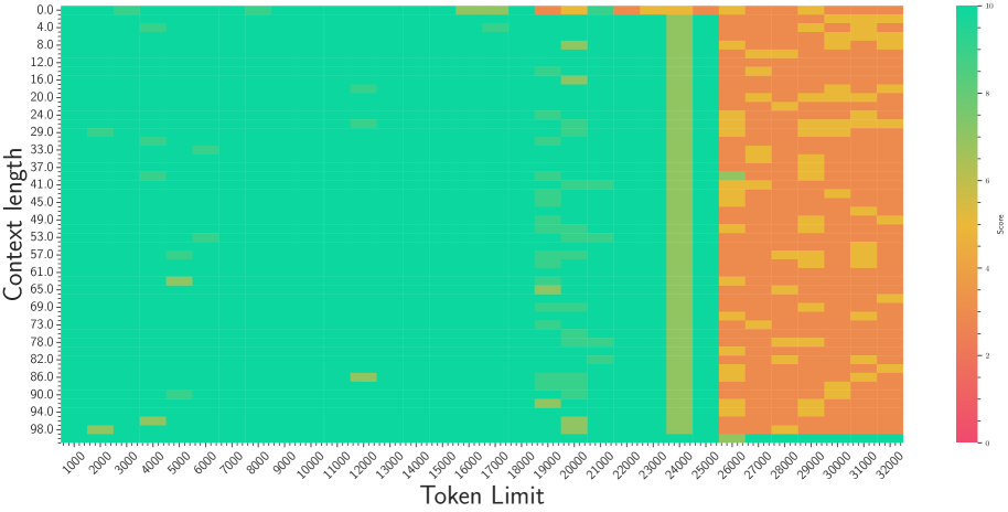
### Visual Description
# Technical Data Extraction: Performance Heatmap
## 1. Document Overview
This image is a technical heatmap visualization representing the performance "Score" of a system (likely a Large Language Model) across two variables: **Token Limit** (x-axis) and **Context length** (y-axis).
## 2. Component Isolation
### A. Header/Title
* No explicit title text is present within the image frame.
### B. Main Chart Area (Heatmap)
* **Type:** 2D Heatmap Grid.
* **X-Axis (Horizontal):** labeled "**Token Limit**".
* **Range:** 1,000 to 32,000.
* **Major Markers:** 1000, 2000, 3000, 4000, 5000, 6000, 7000, 8000, 9000, 10000, 11000, 12000, 13000, 14000, 15000, 16000, 17000, 18000, 19000, 20000, 21000, 22000, 23000, 24000, 25000, 26000, 27000, 28000, 29000, 30000, 31000, 32000.
* **Y-Axis (Vertical):** labeled "**Context length**".
* **Range:** 0.0 to 98.0 (likely representing percentage depth or a specific index).
* **Major Markers:** 0.0, 4.0, 8.0, 12.0, 16.0, 20.0, 24.0, 29.0, 33.0, 37.0, 41.0, 45.0, 49.0, 53.0, 57.0, 61.0, 65.0, 69.0, 73.0, 78.0, 82.0, 86.0, 90.0, 94.0, 98.0.
### C. Legend (Color Bar)
* **Location:** Right-hand side [x: far right, y: centered vertically].
* **Label:** "Score".
* **Scale:** 0 to 10.
* **Color Mapping:**
* **10 (Top):** Bright Teal/Cyan (High Performance).
* **5-7 (Middle):** Yellow/Light Green (Moderate Performance).
* **0-3 (Bottom):** Red/Orange (Low Performance).
---
## 3. Trend Verification and Data Analysis
### Visual Trend Analysis
1. **Stability Zone (1,000 - 18,000 Token Limit):** The chart is predominantly solid teal (Score 10). This indicates near-perfect performance regardless of the "Context length" depth within this range.
2. **Transition Zone (19,000 - 24,000 Token Limit):** The teal color begins to break. We see vertical bands of lighter green and yellow, particularly around the 24,000 mark, suggesting a degradation in performance as the token limit increases.
3. **Failure Zone (25,000 - 32,000 Token Limit):** There is a sharp, vertical "cliff" at the 25,000 mark. Beyond this point, the majority of the grid turns orange/yellow (Score ~3-5).
4. **Bottom Edge Exception:** Interestingly, at the very bottom of the chart (Context length 98.0+), there is a horizontal teal line that persists even into the failure zone, suggesting high performance at the very end of the context regardless of the token limit.
### Key Data Points & Anomalies
* **Perfect Performance:** Found consistently between Token Limits 1,000 and 15,000.
* **The "Cliff":** Performance drops significantly once the Token Limit exceeds **25,000**.
* **Specific Anomalies (Noise):**
* Small yellow/orange blips appear at [Token Limit 2000, Context 98.0].
* A yellow blip at [Token Limit 12000, Context 86.0].
* A yellow blip at [Token Limit 5000, Context 65.0].
* **Vertical Banding:** A distinct vertical band of lower performance (Score ~7-8, light green) is visible at the **24,000 Token Limit** column across almost all Context lengths.
---
## 4. Summary Table of Performance
| Token Limit Range | Context Length Range | Average Score (Visual Est.) | Performance Description |
| :--- | :--- | :--- | :--- |
| 1,000 - 18,000 | 0.0 - 98.0 | 10 | **Optimal:** Consistent high performance. |
| 19,000 - 24,000 | 0.0 - 98.0 | 7 - 9 | **Degrading:** Increasing noise and lower scores. |
| 25,000 - 32,000 | 0.0 - 94.0 | 3 - 5 | **Poor:** Significant performance drop-off. |
| 25,000 - 32,000 | 98.0 | 10 | **Anomaly:** High performance at maximum depth. |
## 5. Language Declaration
The text in this image is entirely in **English**.
</details>
Figure 11: Llama2-7B-Base with base=2e5 fine-tuned on 32k context (original context=4096)
<details>
<summary>x30.png Details</summary>
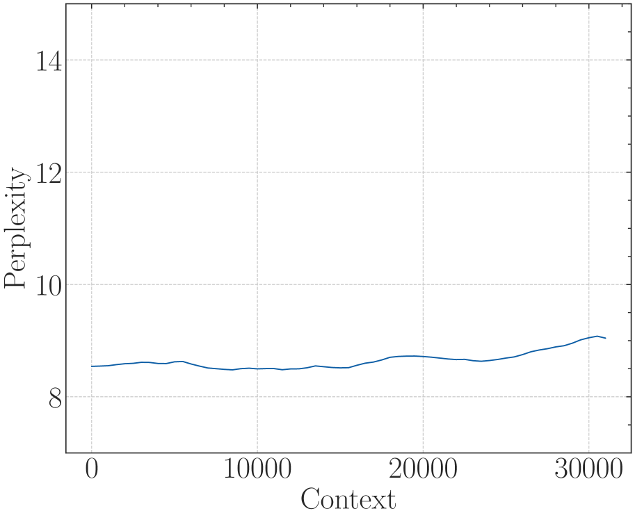
### Visual Description
# Technical Document Extraction: Perplexity vs. Context Chart
## 1. Component Isolation
* **Header:** None present.
* **Main Chart Area:** A line graph plotted on a Cartesian coordinate system with a light gray dashed grid.
* **Axes:**
* **Y-Axis (Vertical):** Labeled "Perplexity".
* **X-Axis (Horizontal):** Labeled "Context".
* **Footer:** None present.
## 2. Axis and Label Extraction
### Y-Axis: Perplexity
* **Label:** Perplexity
* **Major Tick Markers:** 8, 10, 12, 14
* **Minor Tick Markers:** Present at intervals of 0.5 units (e.g., 7.5, 8.5, 9.5, etc.).
* **Range:** The visible scale starts at approximately 7.0 and ends at 15.0.
### X-Axis: Context
* **Label:** Context
* **Major Tick Markers:** 0, 10000, 20000, 30000
* **Minor Tick Markers:** Present at intervals of 2000 units (e.g., 2000, 4000, 6000, 8000).
* **Range:** The visible scale starts at 0 and ends slightly past 30000 (approx. 32000).
## 3. Data Series Analysis
### Series 1: Blue Line
* **Color:** Dark Blue (#1f4e79 approx.)
* **Trend Verification:** The line exhibits a "flat-to-slightly-rising" trend. It begins with minor oscillations between 0 and 15,000 context, maintains a very stable baseline, and shows a gradual, steady upward slope starting after the 25,000 context mark.
* **Key Data Points (Estimated):**
| Context | Perplexity (Approx.) |
| :--- | :--- |
| 0 | 8.5 |
| 5,000 | 8.6 |
| 10,000 | 8.5 |
| 15,000 | 8.5 |
| 20,000 | 8.7 |
| 25,000 | 8.7 |
| 30,000 | 9.1 |
| 31,000 | 9.0 |
## 4. Summary of Information
This chart illustrates the relationship between "Context" (likely context window size in a Large Language Model) and "Perplexity" (a measurement of how well a probability model predicts a sample).
The most significant technical takeaway is the **stability of the model**. While many models see a sharp increase in perplexity (degradation in performance) as context length increases, this specific data shows that the perplexity remains remarkably consistent between 8.5 and 9.1 across a context range of 0 to 30,000+ tokens. The slight upward trend at the end suggests the beginning of a performance trade-off as the context window reaches its upper limits.
</details>
<details>
<summary>x31.png Details</summary>
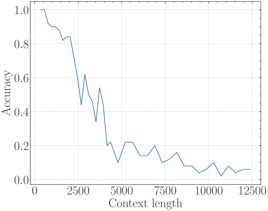
### Visual Description
# Technical Document Extraction: Accuracy vs. Context Length Chart
## 1. Component Isolation
* **Header:** None present.
* **Main Chart Area:** A line graph plotted on a Cartesian coordinate system with a light gray dashed grid.
* **Footer/Axes:** Contains the X-axis label "Context length" and the Y-axis label "Accuracy".
## 2. Axis and Label Extraction
* **Y-Axis (Vertical):**
* **Label:** Accuracy
* **Scale:** 0.0 to 1.0
* **Major Tick Markers:** 0.0, 0.2, 0.4, 0.6, 0.8, 1.0
* **X-Axis (Horizontal):**
* **Label:** Context length
* **Scale:** 0 to 12500
* **Major Tick Markers:** 0, 2500, 5000, 7500, 10000, 12500
## 3. Data Series Analysis
* **Series Name:** Not explicitly labeled (Single series).
* **Color:** Dark Blue.
* **Trend Verification:** The line shows a strong **negative correlation**. It begins at a maximum accuracy of 1.0 at the shortest context length and slopes sharply downward. There is significant volatility (jagged peaks and valleys) between context lengths 2500 and 5000. After 5000, the decline continues at a shallower rate, eventually flattening out near the 0.0 to 0.1 accuracy range as it approaches a context length of 12500.
## 4. Data Point Extraction (Estimated)
Based on the visual alignment with the grid and axis markers:
| Context Length (X) | Accuracy (Y) | Observations |
| :--- | :--- | :--- |
| ~500 | 1.0 | Peak performance |
| ~1000 | 0.9 | Initial drop |
| ~2000 | 0.84 | Local plateau |
| ~2500 | 0.6 | Sharp decline begins |
| ~2700 | 0.44 | Local minimum |
| ~3000 | 0.62 | Significant recovery spike |
| ~3500 | 0.34 | Sharp drop |
| ~3800 | 0.54 | Secondary recovery spike |
| ~4200 | 0.2 | Drop below 0.25 threshold |
| 5000 | ~0.1 | Local minimum |
| 5000 - 6000 | 0.22 | Small plateau/recovery |
| 7500 | ~0.1 | Continued decline |
| 10000 | ~0.05 | Near-zero accuracy |
| 12500 | ~0.06 | Final data point; terminal low |
## 5. Summary of Information
This chart illustrates the performance degradation of a system (likely a Large Language Model or similar information retrieval system) as the input "Context length" increases.
* **High Performance Zone:** Context lengths < 2000 (Accuracy > 0.8).
* **Transition/Instability Zone:** Context lengths 2500 to 4500 (Accuracy fluctuates wildly between 0.6 and 0.2).
* **Failure Zone:** Context lengths > 5000 (Accuracy consistently remains below 0.2, indicating the system loses the ability to process or retrieve information accurately at this scale).
</details>
<details>
<summary>x32.png Details</summary>
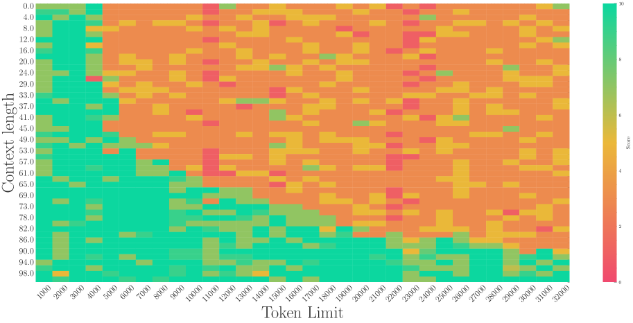
### Visual Description
# Technical Document Extraction: Performance Heatmap Analysis
## 1. Document Overview
This image is a technical heatmap chart visualizing the relationship between two variables—**Token Limit** and **Context Length**—and their resulting **Score**. The chart uses a color gradient to represent performance levels across a 32x26 grid of data points.
## 2. Component Isolation
### A. Header / Metadata
* **Language:** English.
* **Title:** None explicitly provided in the image.
### B. Main Chart Area (Data Visualization)
* **Type:** Heatmap.
* **X-Axis (Horizontal):** Labeled "**Token Limit**".
* **Range:** 1,000 to 32,000.
* **Intervals:** Increments of 1,000 (32 distinct columns).
* **Y-Axis (Vertical):** Labeled "**Context length**".
* **Range:** 0.0 to 98.0.
* **Intervals:** Non-uniform increments (0.0, 4.0, 8.0, 12.0, 16.0, 20.0, 24.0, 29.0, 33.0, 37.0, 41.0, 45.0, 49.0, 53.0, 57.0, 61.0, 65.0, 69.0, 73.0, 78.0, 82.0, 86.0, 90.0, 94.0, 98.0). There are 26 distinct rows.
### C. Legend (Spatial Grounding: Right Side [x=far right, y=centered])
* **Label:** "Score"
* **Scale:** 0 to 10.
* **Color Mapping:**
* **10 (Top):** Bright Teal/Green (High Performance).
* **8:** Light Green.
* **6:** Yellow/Gold.
* **4:** Orange.
* **2:** Light Red/Coral.
* **0 (Bottom):** Deep Pink/Magenta (Low Performance).
---
## 3. Trend Verification and Data Analysis
### Visual Trend Description
The heatmap displays a distinct diagonal "frontier" or boundary.
* **High Score Region (Teal/Green):** Concentrated in the bottom-left quadrant. This indicates that high scores are achieved when the **Token Limit** is low and the **Context length** is high, or when both are relatively low.
* **Low Score Region (Orange/Red):** Concentrated in the top-right quadrant. As the **Token Limit** increases (moving right) and the **Context length** decreases (moving up), the performance score generally degrades.
* **Degradation Pattern:** The transition from Teal (10) to Orange (4) is sharpest along a diagonal line starting roughly at [Token Limit: 5000, Context length: 0.0] and ending at [Token Limit: 32000, Context length: 90.0].
### Key Data Observations
1. **Stability Zone:** For Token Limits between 1,000 and 4,000, the score remains consistently high (Teal, Score ~10) across almost all Context lengths.
2. **The "Cliff":** At a Token Limit of 5,000, there is a significant drop-off in performance for Context lengths above 45.0.
3. **Anomalies:**
* There are scattered "noise" pixels of yellow/green within the orange field (e.g., at Token Limit 29,000, Context length 45.0).
* There are scattered "noise" pixels of red (Score ~2) primarily in the center-right of the chart (e.g., Token Limit 11,000, Context length 57.0).
4. **Bottom Edge Performance:** Interestingly, at the very highest Context lengths (94.0 - 98.0), the model maintains a high score (Teal) even as the Token Limit increases up to approximately 20,000, before becoming more erratic.
---
## 4. Data Table Reconstruction (Representative Sample)
Due to the 32x26 grid size (832 data points), a representative sample of the corners and center is provided:
| Context Length \ Token Limit | 1,000 | 8,000 | 16,000 | 24,000 | 32,000 |
| :--- | :--- | :--- | :--- | :--- | :--- |
| **0.0** | Teal (10) | Orange (4) | Orange (4) | Orange (4) | Orange (4) |
| **24.0** | Teal (10) | Orange (4) | Orange (4) | Orange (4) | Orange (4) |
| **49.0** | Teal (10) | Orange (4) | Yellow (6) | Orange (4) | Orange (4) |
| **73.0** | Teal (10) | Teal (10) | Orange (4) | Orange (4) | Orange (4) |
| **98.0** | Teal (10) | Teal (10) | Teal (10) | Teal (10) | Teal (10) |
---
## 5. Summary of Findings
The chart illustrates a performance trade-off. The system performs optimally (Score 10) in a "safe zone" defined by lower token limits or very high context lengths. There is a large "failure zone" (Score 4) occupying the upper-right majority of the graph, where increasing the token limit while maintaining a low-to-mid context length results in significantly lower scores.
</details>
Figure 12: Baichuan2-7B-Base with base=1e4 fine-tuned on 32k context (original context=4096)
<details>
<summary>x33.png Details</summary>

### Visual Description
# Technical Document Extraction: Perplexity vs. Context Size Chart
## 1. Image Overview
This image is a line graph illustrating the relationship between "Perplexity" and "Context size" for a computational model (likely a Large Language Model). The chart uses a clean, academic style with a serif font and a light gray grid.
## 2. Component Isolation
### Header/Title
* **Content:** None present.
### Main Chart Area
* **Background:** White with a light gray dashed grid.
* **Grid Lines:** Vertical grid lines occur every 10,000 units on the x-axis. Horizontal grid lines occur every 2 units on the y-axis.
* **Data Series:** A single solid dark blue line.
### Axis Labels and Markers
* **Y-Axis (Vertical):**
* **Label:** "Perplexity" (oriented vertically).
* **Scale:** 6 to 15 (visible range).
* **Major Tick Marks:** 6, 8, 10, 12, 14.
* **Minor Tick Marks:** Present between major ticks, indicating increments of 1 unit.
* **X-Axis (Horizontal):**
* **Label:** "Context size".
* **Scale:** 0 to approximately 32,000.
* **Major Tick Marks:** 0, 10000, 20000, 30000.
* **Minor Tick Marks:** Present at intervals of 2,500 units.
### Legend
* **Location:** None present. As there is only one data series, the blue line represents the primary metric.
---
## 3. Data Extraction and Trend Analysis
### Trend Verification
* **Series 1 (Dark Blue Line):** The line begins at a Context size of 0 with a Perplexity value slightly above 7. It remains remarkably stable and flat for the first 15,000 units, showing a very slight downward dip before recovering. After 15,000, the line exhibits a very gradual upward slope, ending just below the 8.0 mark at a context size of 32,000.
### Estimated Data Points
Based on the grid intersections and axis markers, the following data points are extracted:
| Context size (x) | Perplexity (y) | Observations |
| :--- | :--- | :--- |
| 0 | ~7.3 | Starting point. |
| 5,000 | ~7.3 | Stable. |
| 10,000 | ~7.2 | Slightest local minimum. |
| 15,000 | ~7.4 | Beginning of very gradual ascent. |
| 20,000 | ~7.5 | Continued gradual ascent. |
| 25,000 | ~7.6 | Continued gradual ascent. |
| 30,000 | ~7.7 | Peak value reached. |
| 32,000 | ~7.7 | Final data point; shows high stability across long context. |
---
## 4. Technical Summary
The chart demonstrates the **stability of model performance** (measured by Perplexity) as the input **Context size** increases from 0 to 32,000 tokens.
In language modeling, lower perplexity indicates better predictive performance. The data shows that the model maintains a consistent perplexity level (varying only between approximately 7.2 and 7.7) even as the context window expands to 32k. This suggests the model architecture is effective at handling long-range dependencies without significant degradation in its internal probability distributions.
</details>
<details>
<summary>x34.png Details</summary>
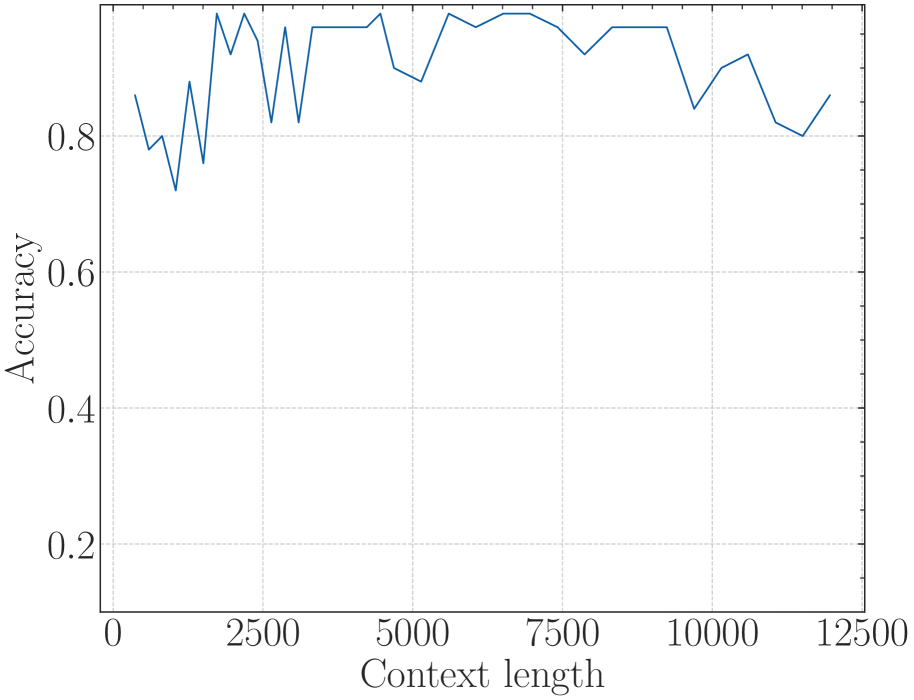
### Visual Description
# Technical Document Extraction: Accuracy vs. Context Length Chart
## 1. Component Isolation
* **Header:** None present.
* **Main Chart Area:** A line graph plotted on a Cartesian coordinate system with a light-gray dashed grid.
* **Y-Axis (Vertical):** Labeled "Accuracy" with numerical markers from 0.2 to 0.8.
* **X-Axis (Horizontal):** Labeled "Context length" with numerical markers from 0 to 12500.
* **Legend:** No explicit legend is present; the chart contains a single data series represented by a solid dark blue line.
---
## 2. Axis and Label Extraction
* **Y-Axis Title:** Accuracy
* **Y-Axis Markers:** 0.2, 0.4, 0.6, 0.8 (Note: The axis extends to 1.0, though the 1.0 label is not explicitly printed, the grid line exists at the top).
* **X-Axis Title:** Context length
* **X-Axis Markers:** 0, 2500, 5000, 7500, 10000, 12500.
---
## 3. Data Series Analysis
### Trend Verification
The data series (dark blue line) represents the relationship between context length and accuracy.
* **Initial Phase (0 - 2500):** High volatility. The line exhibits sharp "sawtooth" fluctuations, starting around 0.85, dropping to a local minimum near 0.7, and spiking back up.
* **Middle Phase (2500 - 9000):** Relative stability at high performance. The line plateaus near the top of the y-axis (approx. 0.95 - 0.98) with minor dips around the 5000 mark.
* **Final Phase (9000 - 12500):** Gradual decline. The line shows a downward trend, dropping from its peak plateau toward the 0.8 accuracy mark as context length approaches 12500.
### Estimated Data Points
*Values are estimated based on grid alignment.*
| Context Length (X) | Accuracy (Y) | Observations |
| :--- | :--- | :--- |
| ~500 | ~0.86 | Starting point |
| ~1000 | ~0.72 | Local minimum in early phase |
| ~2000 | ~0.98 | Early peak |
| ~2500 | ~0.82 | Sharp dip |
| ~4500 | ~0.98 | Peak plateau begins |
| ~5000 | ~0.88 | Mid-range dip |
| ~6000 - 8000 | ~0.98 | Sustained maximum accuracy |
| ~9500 | ~0.84 | Significant drop |
| ~10500 | ~0.92 | Brief recovery |
| ~11500 | ~0.80 | Final local minimum |
| ~12000 | ~0.86 | Ending point |
---
## 4. Technical Summary
This chart illustrates the performance of a system (likely a Large Language Model or similar NLP architecture) where **Accuracy** is measured against varying **Context lengths**.
The system performs best in the "Goldilocks zone" between context lengths of **4,000 and 9,000**, where accuracy remains consistently near its peak (estimated >95%). Performance is unstable with very short contexts (<2,500) and begins to degrade noticeably as the context length exceeds 10,000, suggesting a "lost in the middle" or "context exhaustion" effect common in sequence modeling.
</details>
<details>
<summary>x35.png Details</summary>
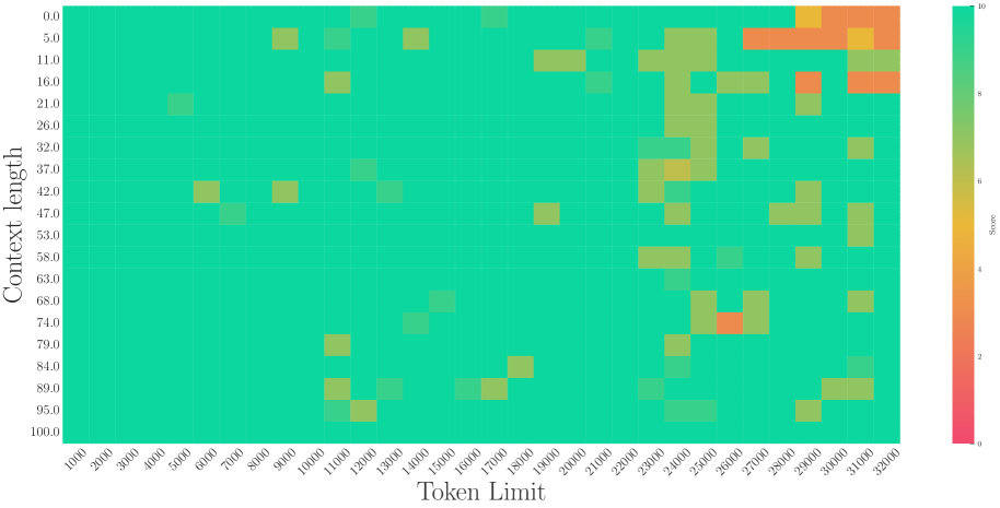
### Visual Description
# Technical Data Extraction: Heatmap Analysis
## 1. Document Overview
This image is a technical heatmap visualization, likely representing the performance of a Large Language Model (LLM) across varying context lengths and token limits. It evaluates a "Score" metric based on two primary dimensions.
## 2. Component Isolation
### A. Header/Metadata
* **Language:** English.
* **Title:** None present in the image.
### B. Main Chart Area (Heatmap)
* **Y-Axis (Vertical):** labeled **"Context length"**.
* **Scale:** 0.0 to 100.0.
* **Markers:** 0.0, 5.0, 11.0, 16.0, 21.0, 26.0, 32.0, 37.0, 42.0, 47.0, 53.0, 58.0, 63.0, 68.0, 74.0, 79.0, 84.0, 89.0, 95.0, 100.0.
* **X-Axis (Horizontal):** labeled **"Token Limit"**.
* **Scale:** 1000 to 32000.
* **Markers (at 1000 intervals):** 1000, 2000, 3000, 4000, 5000, 6000, 7000, 8000, 9000, 10000, 11000, 12000, 13000, 14000, 15000, 16000, 17000, 18000, 19000, 20000, 21000, 22000, 23000, 24000, 25000, 26000, 27000, 28000, 29000, 30000, 31000, 32000.
### C. Legend (Right Side)
* **Spatial Placement:** Located on the far right.
* **Label:** **"Score"**.
* **Scale:** 0 to 10.
* **Color Gradient:**
* **10 (Top):** Bright Teal/Green (Indicates perfect/high performance).
* **5-7 (Middle):** Yellow/Olive (Indicates moderate performance).
* **0-3 (Bottom):** Red/Orange (Indicates poor/low performance).
---
## 3. Trend Verification and Data Extraction
### General Trend Analysis
The heatmap is predominantly **Teal (Score 10)**, indicating high performance across the majority of the tested parameters. However, there is a distinct degradation in performance (shifting toward yellow and orange) concentrated in the **upper-right quadrant** (low Context Length, high Token Limit) and scattered noise in the **far-right columns**.
</details>
Figure 13: Baichuan2-7B-Base with base=2e5 fine-tuned on 32k context (original context=4096)
<details>
<summary>x36.png Details</summary>

### Visual Description
# Technical Document Extraction: Perplexity vs. Context Chart
## 1. Component Isolation
* **Header:** None present.
* **Main Chart Area:** A line graph plotted on a Cartesian coordinate system with a light gray dashed grid.
* **Axes:**
* **Y-Axis (Vertical):** Labeled "Perplexity".
* **X-Axis (Horizontal):** Labeled "Context".
* **Legend:** None present.
## 2. Axis Details and Markers
### Y-Axis: Perplexity
* **Label:** Perplexity (oriented vertically).
* **Scale:** Linear.
* **Major Tick Marks:** 8, 10, 12, 14.
* **Minor Tick Marks:** Present between major ticks (representing increments of 1 unit, with smaller sub-ticks likely representing 0.5 or 0.2 units).
* **Range:** The visible axis starts at approximately 7 and extends to 15.
### X-Axis: Context
* **Label:** Context (oriented horizontally).
* **Scale:** Linear.
* **Major Tick Marks:** 0, 10000, 20000, 30000.
* **Range:** The visible axis starts at 0 and extends slightly past 30000 (to approximately 32000).
## 3. Data Series Analysis
### Series 1: Blue Line
* **Color:** Dark Blue.
* **Trend Verification:** The line exhibits a relatively stable, slightly oscillating horizontal trend for the first two-thirds of the chart, followed by a gradual upward slope in the final third.
* **0 to 15,000 Context:** The line fluctuates narrowly between approximately 8.5 and 8.7.
* **15,000 to 20,000 Context:** The line shows a slight upward trend, peaking near 8.8.
* **20,000 to 25,000 Context:** The line dips slightly and stabilizes around 8.7.
* **25,000 to 31,000 Context:** The line shows a consistent upward trend, reaching its maximum value.
### Estimated Data Points (Visual Extraction)
| Context (X) | Perplexity (Y) |
| :--- | :--- |
| 0 | ~8.55 |
| 5,000 | ~8.65 |
| 10,000 | ~8.50 |
| 15,000 | ~8.55 |
| 20,000 | ~8.75 |
| 25,000 | ~8.70 |
| 30,000 | ~9.10 |
| 31,000 (End) | ~9.05 |
## 4. Summary of Information
This chart illustrates the relationship between "Context" (likely context window size in a machine learning model) and "Perplexity" (a measurement of how well a probability distribution or probability model predicts a sample).
The data indicates that the model maintains a very stable perplexity (between 8.5 and 8.8) for context lengths up to approximately 25,000. Beyond 25,000, there is a measurable but gradual increase in perplexity, suggesting a slight degradation in predictive performance as the context window reaches its maximum observed limit of ~31,000.
</details>
<details>
<summary>x37.png Details</summary>
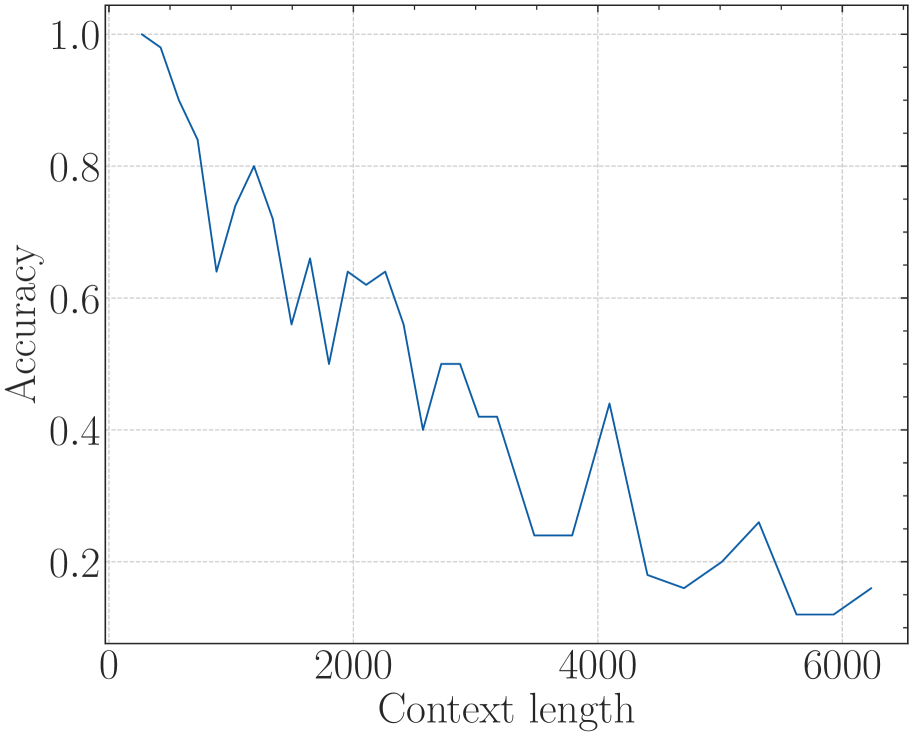
### Visual Description
# Technical Document Extraction: Accuracy vs. Context Length
## 1. Image Classification and Overview
This image is a **line chart** depicting the relationship between model performance (Accuracy) and the amount of input data (Context length). The chart uses a dark blue line plotted against a light gray dashed grid.
## 2. Component Isolation
### Header/Title
* **Content:** None present.
### Main Chart Area
* **Y-Axis Label:** "Accuracy" (Vertical, left-aligned).
* **X-Axis Label:** "Context length" (Horizontal, bottom-centered).
* **Y-Axis Scale:** Linear, ranging from 0.0 to 1.0 with major ticks every 0.2.
* **X-Axis Scale:** Linear, ranging from 0 to 6000 with major ticks every 2000. Minor ticks are present every 500 units.
* **Grid:** Light gray dashed lines corresponding to major axis markers.
### Legend
* **Content:** None present. There is only a single data series.
---
## 3. Data Series Analysis
### Trend Verification
* **Series Name:** Accuracy (implied).
* **Color:** Dark Blue.
* **Visual Trend:** The line shows a **strong negative correlation**. It begins at the maximum value (1.0) at the shortest context length and follows a jagged, downward trajectory. While there are local "spikes" or recoveries (notably around context lengths 1200, 2000, and 4100), the overall macro trend is a significant decline as context length increases, eventually bottoming out below 0.2.
### Data Point Extraction (Estimated)
Based on the grid intersections and axis markers, the following data points represent the trajectory of the line:
| Context Length (X) | Accuracy (Y) | Notes |
| :--- | :--- | :--- |
| ~250 | 1.00 | Starting point / Peak accuracy |
| ~500 | 0.98 | Slight initial dip |
| ~800 | 0.85 | |
| ~1000 | 0.64 | Significant local drop |
| ~1250 | 0.80 | Local recovery peak |
| ~1500 | 0.56 | |
| ~1700 | 0.66 | |
| ~1850 | 0.50 | |
| ~2000 | 0.64 | Local recovery peak |
| ~2300 | 0.64 | Plateau |
| ~2600 | 0.40 | |
| ~2800 | 0.50 | |
| ~3000 | 0.50 | Plateau |
| ~3200 | 0.42 | |
| ~3500 | 0.24 | |
| ~3800 | 0.24 | Plateau |
| ~4100 | 0.44 | Significant late-stage spike |
| ~4400 | 0.18 | |
| ~4700 | 0.16 | Lowest point in series |
| ~5300 | 0.26 | |
| ~5600 | 0.12 | |
| ~5900 | 0.12 | Final plateau |
| ~6200 | 0.16 | Final data point |
---
## 4. Summary of Findings
The chart demonstrates a "Lost in the Middle" or context-exhaustion phenomenon. The model maintains near-perfect accuracy (1.0) at very short context lengths (under 500). However, as the context length increases toward 6000, the accuracy degrades significantly, fluctuating but ultimately losing approximately 85% of its initial performance, ending at an accuracy level between 0.12 and 0.16.
</details>
<details>
<summary>x38.png Details</summary>
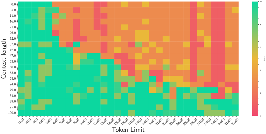
### Visual Description
# Technical Data Extraction: Performance Heatmap
## 1. Document Overview
This image is a technical heatmap visualizing the relationship between two variables—**Token Limit** and **Context Length**—and their resulting effect on a **Score**. The chart likely represents the performance of a Large Language Model (LLM) or a similar data processing system across varying input constraints.
## 2. Component Isolation
### A. Header / Metadata
* **Language:** English.
* **Title:** None explicitly provided in the image.
### B. Main Chart (Heatmap)
* **Y-Axis (Vertical):** Labeled **"Context length"**.
* **Scale:** 0.0 to 100.0.
* **Markers:** 0.0, 5.0, 11.0, 16.0, 21.0, 26.0, 32.0, 37.0, 42.0, 47.0, 53.0, 58.0, 63.0, 68.0, 74.0, 79.0, 84.0, 89.0, 95.0, 100.0.
* **X-Axis (Horizontal):** Labeled **"Token Limit"**.
* **Scale:** 1,000 to 32,000.
* **Markers:** 1000, 2000, 3000, 4000, 5000, 6000, 7000, 8000, 9000, 10000, 11000, 12000, 13000, 14000, 15000, 16000, 17000, 18000, 19000, 20000, 21000, 22000, 23000, 24000, 25000, 26000, 27000, 28000, 29000, 30000, 31000, 32000.
### C. Legend (Color Bar)
* **Location:** Right side of the chart.
* **Label:** **"Score"**.
* **Scale:** 0 to 10.
* **Color Mapping:**
* **10 (Top):** Bright Green (High Performance).
* **5-7 (Middle):** Yellow/Orange (Moderate Performance).
* **0 (Bottom):** Red/Pink (Low Performance).
---
## 3. Trend Verification & Data Analysis
### Visual Trend Description
The heatmap shows a distinct diagonal degradation of performance.
* **High Performance Zone (Green):** Concentrated in the bottom-left quadrant (Low Token Limit, High Context Length) and the far left edge (Low Token Limit across all Context Lengths).
* **Low Performance Zone (Red/Orange):** Concentrated in the top-right quadrant (High Token Limit, Low Context Length).
* **Transition Zone:** There is a "noisy" diagonal boundary where the score fluctuates between green, yellow, and red as the Token Limit increases and Context Length decreases.
### Key Data Observations
1. **Stability at Low Token Limits:** For Token Limits between 1,000 and 5,000, the score remains predominantly green (Score ~8-10) regardless of the Context Length.
2. **Degradation Threshold:** A significant performance drop (transition to orange/red) begins to appear around the 6,000 Token Limit mark for Context Lengths above 32.0.
3. **Critical Failure Zones:**
* At a Token Limit of 32,000, the score is consistently low (orange/red) for Context Lengths between 0.0 and 74.0.
* Vertical "stripes" of red (Score 0-2) are visible at specific Token Limits, notably around 26,000 and 29,000, suggesting systemic failures at those specific intervals.
4. **Anomalies:** There are scattered green pixels within the high-token/low-context "red zone" (e.g., at Token Limit 18,000 / Context Length 37.0), indicating inconsistent performance or outliers.
---
## 4. Data Table Reconstruction (Representative Samples)
Due to the high density of the heatmap (approx. 20x32 grid), the following table represents the general score distribution:
| Context Length \ Token Limit | 1,000 | 8,000 | 16,000 | 24,000 | 32,000 |
| :--- | :--- | :--- | :--- | :--- | :--- |
| **0.0** | Green (10) | Orange (4) | Orange (4) | Orange (4) | Orange (4) |
| **26.0** | Green (10) | Red (2) | Orange (4) | Orange (4) | Orange (4) |
| **53.0** | Green (10) | Green (10) | Red (2) | Orange (4) | Orange (4) |
| **79.0** | Green/Yellow (8) | Green (10) | Green (10) | Orange (5) | Red (2) |
| **100.0** | Green (10) | Green (10) | Green (10) | Green (10) | Green (10) |
---
## 5. Summary of Findings
The system demonstrates an inverse relationship between Token Limit and Context Length performance. It is most reliable (Score 10) when the Context Length is high (near 100.0) or the Token Limit is very low (under 5,000). The most significant performance "dead zone" occurs when the Token Limit exceeds 20,000 and the Context Length is below 50.0.
</details>
Figure 14: Qwen1.5-7B-Base (Bai et al., 2023) with base=1e4 fine-tuned on 32k context (original context=4096)