2405.17430

# Matryoshka Multimodal Models ## Abstract Large Multimodal Models (LMMs) such as LLaVA have shown strong performance in visual-linguistic reasoning. These models first embed images into a fixed large number of visual tokens and then feed them into a Large Language Model (LLM). However, this design causes an excessive number of tokens for dense visual scenarios such as high-resolution images and videos, leading to great inefficiency. While token pruning and merging methods exist, they produce a single-length output for each image and cannot afford flexibility in trading off information density v.s. efficiency. Inspired by the concept of Matryoshka Dolls, we propose M 3: Matryoshka Multimodal Models, which learns to represent visual content as nested sets of visual tokens that capture information across multiple coarse-to-fine granularities. Our approach offers several unique benefits for LMMs: (1) One can explicitly control the visual granularity per test instance during inference, e.g., adjusting the number of tokens used to represent an image based on the anticipated complexity or simplicity of the content; (2) M 3 provides a framework for analyzing the granularity needed for existing datasets, where we find that COCO-style benchmarks only need around 9 visual tokens to obtain an accuracy similar to that of using all 576 tokens; (3) Our approach provides a foundation to explore the best trade-off between performance and visual token length at the sample level, where our investigation reveals that a large gap exists between the oracle upper bound and current fixed-scale representations. ## 1 Introduction Large Multimodal models (LMMs) [1, 2, 3, 4, 5, 6, 7] have shown strong performance in visual-linguistic understanding and reasoning. Models such as LLaVA [2, 5, 4] first embed the input image with a fixed number of visual tokens, and then feed them as prefix tokens to a Large Language Model (LLM) [8, 9] to reason about the input image. Similar model designs are borrowed in video LMMs [10, 11], where each frame contributes a fixed number of tokens to form the final video representation. In reality, the number of visual tokens can be prohibitively large in the case of high-resolution images, and even more so for long videos. Existing works [10, 4, 12, 13] mainly tackle this issue by increasing the input context length and consequently, feeding a large number e.g., 3-8k of visual tokens into the LLM. This approach has a couple of significant drawbacks: (1) the extremely long context makes both training and inference inefficient; (2) an excessive number of visual tokens can actually harm the LMM’s performance, distracting it from attending to the relevant information, as we show in Sec. 4.3. Several recent works [14, 15, 16] use heuristics to prune and merge visual tokens to reduce the sequence length. However, they produce a single-length output and do not afford control over the final sequence length, which could be useful to trade information density versus efficiency while accounting for resource constraints in the deployment phase. <details> <summary>x1.png Details</summary>  ### Visual Description ## Diagram: Multimodal AI Image Description at Multiple Scales (M³) ### Overview This image is a conceptual diagram illustrating how a multimodal AI system (labeled "M³") can generate textual descriptions of an input image at varying levels of detail or "scales." The diagram uses the metaphor of nested Matryoshka dolls to represent these different scales, with each doll corresponding to a specific descriptive output. The core input is a photograph of a young girl in a restaurant. ### Components/Axes 1. **Header/Title Element:** * **Label:** "M³" (Large, black, sans-serif font, positioned top-center). * **Metaphor:** A row of seven Matryoshka dolls in decreasing size from left to right. Colors from left (largest) to right (smallest): Red, Orange, Yellow, Green, Light Blue, Dark Blue, Purple. Each doll has a heart motif on its front. 2. **Input Image:** * **Position:** Left side, below the doll row. * **Content:** A photograph of a young girl with dark hair, wearing a blue and white striped sweater, sitting at a wooden table in what appears to be a restaurant. She is holding food. On the table are a white paper bag and a blue cup with a Pepsi logo. The background shows a warmly lit, busy interior. 3. **Processing Flow:** * A light blue arrow points from the input image towards the right, indicating the direction of processing by the M³ system. 4. **Output Scales & Descriptions (Legend/Key):** * The diagram defines three specific output scales, each associated with a Matryoshka doll icon and a labeled text box. * **Scale 1 (Xs₁):** * **Icon:** The smallest, purple Matryoshka doll. * **Label:** "Xs₁" (positioned left of the icon). * **Text Box:** Pink background, rounded corners. Contains a brief, general description. * **Scale 2 (Xs₂):** * **Icon:** The second-smallest, dark blue Matryoshka doll. * **Label:** "Xs₂" (positioned left of the icon). * **Text Box:** Light blue background, rounded corners. Contains a more detailed description. * **Ellipsis (...):** Three black dots between Xs₂ and Xsₘ indicate there are intermediate scales not shown. * **Scale M (Xsₘ):** * **Icon:** The largest, red Matryoshka doll. * **Label:** "Xsₘ" (positioned left of the icon). * **Text Box:** Salmon/red background, rounded corners. Contains the most detailed and comprehensive description. 5. **User Prompt:** * **Position:** Top-right corner. * **Element:** A white rounded rectangle with a black border containing the text "Describe this image for me." Next to it is a simple black user icon. ### Detailed Analysis / Content Details * **Textual Transcription of Descriptions:** * **Xs₁ (Pink Box):** "In the heart of a bustling restaurant, a young girl finds solace at a table..." * **Xs₂ (Blue Box):** "In the heart of a bustling restaurant, a young girl with vibrant hair is seated at a wooden table, her attention captivated by the camera..." * **Xsₘ (Red Box):** "In the heart of a bustling restaurant, a young girl with long, dark hair is the center of attention. She's dressed in a blue and white striped sweater, ... The table is adorned with a white paper bag, perhaps holding her meal. A blue Pepsi cup rests on the table ..." * **Progression of Detail:** * **Trend:** As the scale increases (from Xs₁ to Xsₘ), the description becomes significantly more detailed and specific. * **Xs₁:** General scene and subject ("young girl," "bustling restaurant"). * **Xs₂:** Adds specific attributes ("vibrant hair," "wooden table," "attention captivated by the camera"). * **Xsₘ:** Provides precise visual details ("long, dark hair," "blue and white striped sweater," "white paper bag," "blue Pepsi cup") and inferential language ("perhaps holding her meal"). * **Spatial Grounding of Legend:** * The legend (the row of dolls) is positioned at the **top-left** of the diagram. * The output text boxes are arranged vertically on the **right side**, aligned with their corresponding doll icons which are placed to their immediate left. * The color of each text box background (pink, light blue, red) is explicitly matched to the color of its associated Matryoshka doll icon (purple, dark blue, red), creating a clear visual link. ### Key Observations 1. **Hierarchical Metaphor:** The Matryoshka doll is used effectively as a visual metaphor for nested or hierarchical scales of information, where larger dolls (coarser scales) contain smaller, more detailed ones. 2. **Color-Coding Consistency:** The diagram maintains strict color consistency between the doll icons and their corresponding text boxes, ensuring unambiguous mapping. 3. **Detail Gradient:** There is a clear and intentional gradient in descriptive detail, moving from vague to highly specific, which is the core concept being illustrated. 4. **Ellipsis for Implied Continuum:** The use of "..." between Xs₂ and Xsₘ indicates that the system can generate descriptions at many intermediate scales, not just the three shown. ### Interpretation This diagram is a technical illustration of a **multi-scale or hierarchical image captioning system**. The "M³" likely stands for "Multi-scale Multimodal Model" or a similar concept. * **What it Demonstrates:** It shows that a single AI model can process one input image and produce a family of related textual outputs, each tailored to a different level of granularity. This is valuable for applications where the required detail depends on context (e.g., a quick thumbnail alt-text vs. a detailed accessibility description). * **Relationship Between Elements:** The input image is the source. The M³ system (implied by the arrow and title) acts upon it. The Matryoshka dolls symbolize the internal "scales" or "resolutions" at which the model operates. The text boxes are the concrete, human-readable outputs corresponding to each scale. * **Underlying Concept:** The model isn't just generating one description; it's learning a **structured representation** of the image where information is organized by importance or specificity. The largest doll (Xsₘ) represents the most comprehensive representation, containing all the details that are summarized or omitted in the smaller-scale descriptions (Xs₂, Xs₁). This is analogous to how a large Matryoshka doll physically contains all the smaller ones. * **Notable Anomaly/Feature:** The descriptions for Xs₁ and Xs₂ both begin with the identical phrase "In the heart of a bustling restaurant...", suggesting the model may generate a common "scene-setting" clause before diverging into scale-specific details. The Xsₘ description breaks this pattern, starting directly with the subject, which might indicate a different generation strategy for the most detailed scale. 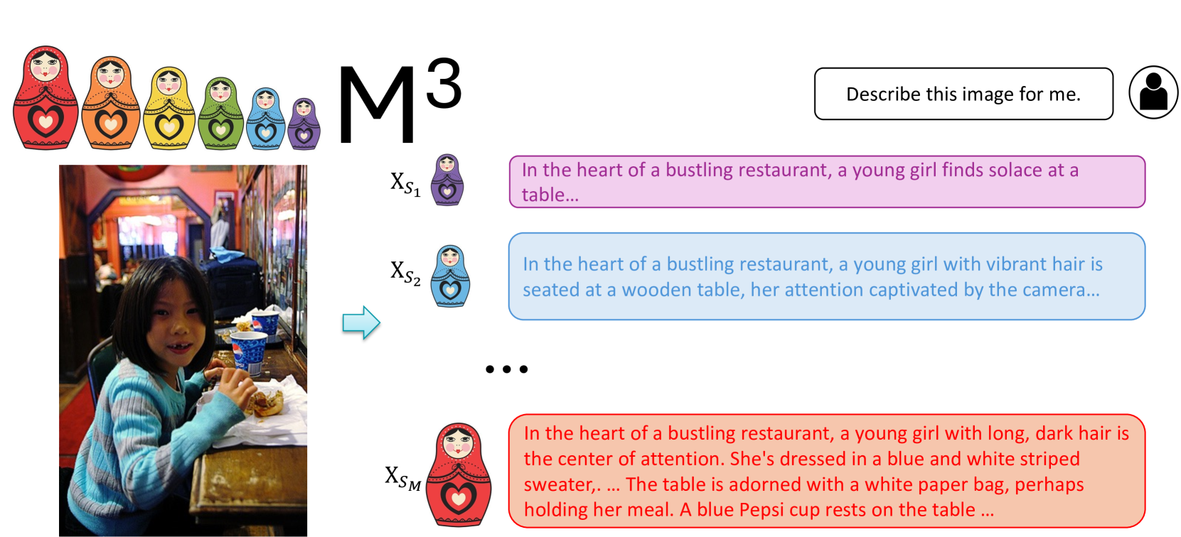</details> Figure 1: Matryoshka Multimodal Models. We enforce the coarser set of visual tokens $X_S_{i-1}$ to be derived from the finer level of visual tokens $X_S_{i}$ . As a result, the granularity of Matryoshka visual tokens gradually changes in a controllable manner. The image is from MSCOCO [17] validation set. Images and videos naturally exhibit a hierarchical structure from coarse to fine details, and our human visual system has evolved to recognize visual information in this coarse to fine manner, as shown by biologists and psychologists decades ago [18, 19]. Can we create a similar structure for LMMs, where within one suite of model weights, the visual content tokens are organized into different scales of granularities? Conceptually, our goal is to learn the visual tokens to have a nested structure, similar to the Matryoshka Doll [20]. Matryoshka Representation Learning (MRL) [20] builds the Matryoshka mechanism over a neural network’s representation vector, where each of the segments with various feature dimensions is capable of handling tasks like classification or retrieval. However, for LMMs, the inefficiency mainly comes from the number of tokens. Thus, inspired by, but different from MRL, our work is motivated to build Matryoshka Multimodal Models upon the token length dimension, so that we can flexibly adjust it. <details> <summary>extracted/5762161/figures/scale_plot_submission.png Details</summary>  ### Visual Description ## Scatter Plot with Line Connections: MMBench Performance vs. Number of Visual Tokens ### Overview This image is a scatter plot with connected lines for two of the data series, illustrating the relationship between the "Number of Visual Tokens" (x-axis) and "MMBench Performance" (y-axis) for several multimodal AI models. The chart compares the performance scaling of different models as the number of visual tokens increases. ### Components/Axes * **X-Axis:** Labeled "Number of Visual Tokens". The scale runs from 0 to 600, with major tick marks at 0, 100, 200, 300, 400, 500, and 600. * **Y-Axis:** Labeled "MMBench Performance". The scale runs from 20 to 70, with major tick marks at 20, 30, 40, 50, 60, and 70. * **Legend:** Located in the bottom-right quadrant of the chart area. It contains six entries: 1. **M³:** Blue solid line with filled circle markers. 2. **LLaVA-1.5:** Orange dashed line with filled circle markers. 3. **Oracle under M³:** A single red filled circle marker. 4. **LLaVA-1.5 Specific Scale:** Green 'X' markers. 5. **Qwen-VL Chat:** A single yellow filled circle marker with a black outline. 6. **InstructBLIP-7B:** A single pink filled circle marker with a black outline. ### Detailed Analysis **Data Series and Trends:** 1. **M³ (Blue Line, Circles):** * **Trend:** The line shows a very steep initial increase in performance as tokens increase from near 0, followed by a rapid plateau. The performance remains nearly constant from approximately 150 tokens onward. * **Approximate Data Points:** * At ~0 tokens: Performance ≈ 59.5 * At ~10 tokens: Performance ≈ 63 * At ~30 tokens: Performance ≈ 65 * At ~150 tokens: Performance ≈ 66.5 * At ~580 tokens: Performance ≈ 66 2. **LLaVA-1.5 (Orange Dashed Line, Circles):** * **Trend:** Similar to M³, it shows a steep initial rise, but starts from a much lower performance baseline. It continues to increase more gradually after the initial jump, showing a slight upward slope even at higher token counts. * **Approximate Data Points:** * At ~0 tokens: Performance ≈ 19.5 * At ~5 tokens: Performance ≈ 45.5 * At ~30 tokens: Performance ≈ 50.5 * At ~150 tokens: Performance ≈ 61.5 * At ~580 tokens: Performance ≈ 64 3. **Individual Model Points:** * **Oracle under M³ (Red Circle):** Positioned at approximately (10, 72). This is the highest performance point on the chart. * **LLaVA-1.5 Specific Scale (Green 'X's):** Three markers are present. * One near (10, 60) * One near (30, 63) * One near (150, 64.5) * **Qwen-VL Chat (Yellow Circle):** Positioned at approximately (260, 60.5). * **InstructBLIP-7B (Pink Circle):** Positioned at approximately (30, 36). ### Key Observations * **Performance Plateau:** Both the M³ and LLaVA-1.5 models exhibit a clear performance plateau. M³ reaches its near-maximum performance with as few as ~150 visual tokens, while LLaVA-1.5 shows slower gains after the initial steep rise. * **Model Comparison:** At every comparable token count, the M³ model significantly outperforms LLaVA-1.5. The gap is largest at very low token counts and narrows slightly as tokens increase. * **Oracle Performance:** The "Oracle under M³" point suggests a theoretical or ideal performance ceiling (~72) that is substantially higher than any achieved by the models shown, even at high token counts. * **Token Efficiency:** M³ appears to be highly token-efficient, achieving over 95% of its peak performance with less than 25% of the maximum displayed token count (150 out of 600). * **Outliers:** The InstructBLIP-7B point is a notable low-performer relative to its token count (~30 tokens, performance ~36), falling well below the trend lines of both M³ and LLaVA-1.5. ### Interpretation This chart demonstrates the critical relationship between visual token count and model performance on the MMBench benchmark. The data suggests that: 1. **Diminishing Returns:** There are strong diminishing returns to adding more visual tokens beyond a certain point (around 150-200 for these models). This implies an efficiency frontier in visual token utilization for these architectures. 2. **Architectural Superiority:** The M³ model architecture is fundamentally more effective at translating visual tokens into benchmark performance than LLaVA-1.5, as evidenced by its higher performance curve at all points and its steeper initial ascent. 3. **Performance Gap to Oracle:** The large gap between the best model performance (~66) and the Oracle point (~72) indicates significant room for improvement in multimodal model design, suggesting current models are not fully leveraging the information available in the visual tokens. 4. **Model-Specific Scaling:** The "LLaVA-1.5 Specific Scale" points (green 'X's) closely follow the main LLaVA-1.5 trend line, suggesting consistent scaling behavior for that model family. The scatter of other models (Qwen-VL, InstructBLIP) highlights the variance in performance and token efficiency across different model designs. In essence, the chart argues that while increasing visual token count improves performance, the choice of model architecture (M³ vs. LLaVA-1.5) is a more significant determinant of both peak performance and token efficiency. The plateau effect also informs practical design choices, suggesting that using a very large number of tokens may not be computationally justified. 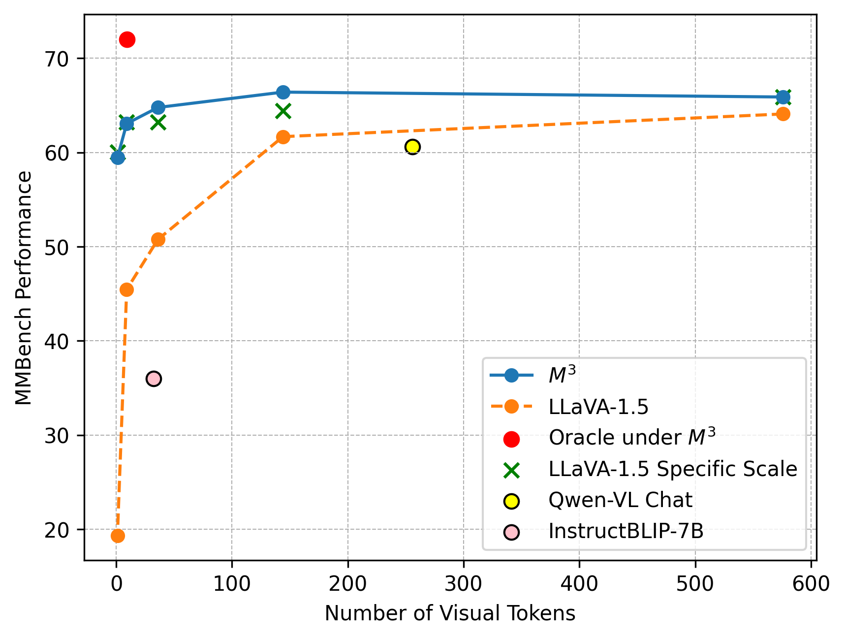</details> Figure 2: MMBench evaluation results under M 3, oracle under LLaVA-1.5- M 3, LLaVA-1.5 with average pooling at inference time, LLaVA-1.5 separately trained for each specific scale, and other methods. M 3 shows as least as good performance as LLaVA trained for each specific scale. A large gap exists between the oracle upperbound and model’s actual performance on a specific scale. Specifically, we propose M 3: Matryoshka Multimodal Models, which enforces an LMM to learn a hierarchy of visual representation granularities at the token sequence level, instead of the feature dimension level as in MRL [20]. With this representation, at inference time, the visual granularity can be flexibly controlled based on specific requirements, e.g., to account for the input image’s information density and efficiency constraints. Our training process is simple and straightforward. During training, we encode the image into $M$ sets of visual tokens from coarse to fine, $X_S_{i}$ , $i=1,⋯,M$ , where the number of visual tokens gradually increases, i.e., $|X_S_{i-1}|<|X_S_{i}|$ . And importantly, the visual tokens in a coarser level are derived from the visual tokens in a finer level, i.e., $X_S_{i-1}⊂X_S_{i}$ , $∀ i$ . In this way, the visual information in $[{X}_S_1,{X}_S_2,⋯,{X}_S_{M}]$ gradually includes more fine-grained details. For example, given a natural image as shown in Figure 1, $X_S_1$ includes high-level semantics such as the restaurant and girl, while $X_S_{M}$ includes more details such as the Pepsi cup and white paper bag. All other training settings, such as the loss function and model architecture, are kept the same as LLaVA [2, 5, 4]. Our approach, M 3, introduces several novel properties and benefits for LMMs. First, our approach can adaptively and efficiently represent visual content. Under one suite of weights, it generates multiple nested sets of visual tokens with different granualarities in information density. This enables flexibility in the number of visual tokens used for any image during inference, enabling control over the best tradeoff between cost and performance based on the image or video content. For example, one can use all visual tokens for images with dense details and use just a few tokens for simpler images. This flexibility can be particularly significant when handling very long visual sequences, such as videos. For instance, given a fixed budget of 2880 visual tokens, a user could represent a video of 2880 frames each with one token or represent the same video by sampling 5 frames each with 576 tokens. Second, our approach can be used as a general framework to evaluate the visual complexity of vision-language datasets or benchmarks, i.e., which level of granularity is needed in order to perform the given task correctly. Surprisingly, we find that most benchmarks, especially those mainly crafted from natural scenes (such as COCO) [21, 22, 23], can be handled well with only $∼ 9$ tokens per image. In contrast, dense visual perception tasks such as document understanding or OCR [24, 25] require a greater amount of tokens ( $144-576$ tokens) per image to handle the task well. The detailed findings are presented in Sec. 4.2. Finally, our approach provides a foundation to tackle a critical task in LMMs: How to use the least amount of visual tokens while answering the visual questions correctly?. Based on the model’s predictions on the test set, we find that compared to full visual tokens, the oracle can use far fewer tokens while performing much better. For example, under six common LMM benchmarks used in LLaVA-NeXT [4], the oracle with the trained M 3 model can use as few as 8.9 visual tokens on average to achieve performance that is 8% points better than LLaVA-NeXT which uses 576 tokens per image grid. This indicates that there is a large room for improvement compared to the oracle upperbound, as we show in Sec. 4.2. To enable further research on adaptive LMMs that learn diverse information granularities, we publicly release our code and models. ## 2 Related Work Large Multimodal Models. Large Language Models (LLMs) like ChatGPT [26], GPT-4 [27], and LLaMA [28] have demonstrated impressive reasoning and generalization capabilities for text. The landscape of LLMs has been significantly transformed by the recent introduction of models that also incorporate visual information, such as GPT-4V(ision) [1]. Building upon open-source LLMs [28, 8], a plethora of multimodal models have made significant strides, spearheaded by models like LLaVA [2, 5] and MiniGPT-4 [3], which combine LLaMA’s [28] language capabilities with a CLIP [29] based image encoder. Recently, LMMs on more tasks and modalities have emerged, such as region level LMMs [30, 31, 32, 33, 34], 3D LMMs [35], and video LMMs [10, 11, 12]. However, existing LMMs typically represent the visual content with a large and fixed number of tokens, which makes it challenging to scale to very long visual sequences such as high-resolution images or long-form videos. In this work, we propose to adaptively and efficiently represent the visual content by learning multiple nested sets of visual tokens, providing flexibility in the number of visual tokens used for any image during inference. Matryoshka Representation Learning. Matryoshka Representation Learning (MRL) [20] addresses the need for flexible representations that can adapt to multiple downstream tasks with varying computational resources. This approach, inspired by the nested nature of Matryoshka dolls, encodes information at different granularities within the same high-dimensional feature vector produced by a neural network. The adaptability of MRL extends across different modalities, including vision (ResNet [36], ViT [37]), vision + language (ALIGN [38]), and language (BERT [39]), demonstrating its versatility and efficiency. Recent work [40] extends MRL to both the text embedding space and the Transformer layers space. Our approach is inspired by MRL, but instead of learning multiple nested embeddings for a high-dimensional feature vector, we learn nested visual tokens along the token length dimension for the visual input. We are the first to show that the idea of Matryosha learning can enable explicit control over the visual granularity of the visual content that an LMM processes. Token Reduction. One of the main causes of inefficiency in recent LMMs is their large number of prefix visual tokens that are fed into the LLM [2, 3]. The quadratic complexity in Transformers [41] is the key issue in scaling the input sequence length for Transformers. Token reduction serves as an effective technique to reduce computational costs in Transformers. Sparse attention methods such as Linformer [42] and ReFormer [43] conduct attention operations within local windows rather than the full context, thereby reducing the quadratic complexity of the vanilla attention operation. Another notable method is Token Merging (ToMe) [14], which utilizes full attention but gradually reduces the number of tokens in each transformer block by selecting the most representative tokens through bipartite matching for the Vision Transformer (ViT). A recent work [44] further studies different families of token reduction methods for ViT. However, prior approaches produce a single length output per input image and do not offer multiple granularities over the reduced token sequence. Our M 3 approach instead learns a multi-granularity, coarse-to-fine token representation within the same model architecture and weights, enabling it to easily be adjusted to various computational or memory constraints. A concurrent work [45] shares a similar spirit with our approach, representing an image with varying numbers of visual tokens using a single set of model weights. While their method reformats the visual tokens into a sequential list via transformation layers, we use average pooling to preserve the spatial structure of the visual tokens, demonstrating effectiveness in our experiments. ## 3 M 3 : Matryoshka Multimodal Models <details> <summary>x2.png Details</summary>  ### Visual Description ## Diagram: Matryoshka Multimodal Models Architecture ### Overview This image is a technical diagram illustrating the architecture of a "Matryoshka Multimodal Model." The system processes an input image and a text prompt to generate a textual description. The core concept, symbolized by Russian nesting dolls (matryoshka), is that the image representation can be encoded at multiple, nested levels of granularity, which are then processed by a Large Language Model (LLM) alongside the text prompt. ### Components/Axes The diagram is organized into a flow from left to right, with distinct input, processing, and output stages. **1. Input Stage (Left Side):** * **Image Input:** A photograph showing a group of people posing in a snowy, outdoor ski facility. Some individuals are holding a green flag. * **Text Prompt Input:** A yellow-bordered box containing: * **Label:** `Text Prompt` * **Icon:** A user silhouette. * **Prompt Text:** `: Describe the scene for me.` **2. Processing Stage (Center):** * **CLIP Image Encoder:** A blue trapezoidal block that receives the input image. An arrow points from it to the multi-granularity representations. * **Granularity Controller:** A blue-bordered box below the encoder, containing: * **Label:** `Granularity Controller` * **Icon:** A hand adjusting a slider. * **Function:** This component controls the level of detail (granularity) extracted from the image by the encoder. * **Multi-Granularity Image Representations:** The output of the CLIP Image Encoder is depicted as multiple rows of colored blocks (pink, blue, red), each associated with a matryoshka doll icon of decreasing size. These are labeled: * `X_S₁` (smallest doll, top row) * `X_S₂` (medium doll, middle row) * `⋮` (vertical ellipsis indicating continuation) * `X_Sₘ` (largest doll, bottom row) * This visually represents a set of image embeddings at different scales or levels of abstraction (`S₁` to `Sₘ`). * **Text Encoder (Implied):** The text prompt is processed into a sequence of yellow blocks, representing its tokenized or embedded form. **3. Integration & Output Stage (Right Side):** * **Large Language Model (LLM):** A large, peach-colored rectangular block. It receives two inputs: 1. The multi-granularity image representations (indicated by a downward arrow from the `X_S` blocks). 2. The encoded text prompt (indicated by a downward arrow from the yellow blocks). * **Generated Output:** An orange-bordered box containing the model's response: * **Icon:** A robot head. * **Output Text:** `: There are a group of people standing in the ski facility, some of them are holding a green flag while other are ...` (The text ends with an ellipsis, indicating continuation). **4. Title & Symbolism:** * **Title:** `Matryoshka Multimodal Models` in large, blue, italicized font at the top center. * **Symbolic Header:** A row of seven colorful matryoshka dolls (red, orange, yellow, green, light blue, dark blue, purple) in the top-left corner, reinforcing the "nested" or hierarchical model concept. ### Detailed Analysis The diagram details a specific multimodal AI pipeline: 1. **Image Encoding:** An image is passed through a CLIP Image Encoder. 2. **Granular Control:** A "Granularity Controller" modulates the encoder to produce not one, but a series of image representations (`X_S₁` through `X_Sₘ`). Each representation corresponds to a different level of detail, metaphorically shown as nested dolls where `X_S₁` is the most compact (coarse) and `X_Sₘ` is the most detailed (fine). 3. **Text Encoding:** A user's text prompt is separately encoded. 4. **Multimodal Fusion:** The set of image representations and the text encoding are fed into a Large Language Model. 5. **Text Generation:** The LLM synthesizes this information to generate a natural language description of the image, as shown in the sample output. ### Key Observations * **Hierarchical Representation:** The core innovation highlighted is the generation of multiple, scale-aware image features (`X_S₁...X_Sₘ`) instead of a single fixed representation. * **Explicit Control:** The "Granularity Controller" is a distinct, user-adjustable component, suggesting the model's output detail can be tuned. * **CLIP-Based:** The image encoder is specified as "CLIP," indicating the use of a contrastive language-image pre-training foundation. * **Flow Clarity:** The data flow is clearly marked with arrows: image → encoder → multi-scale features → LLM, and text prompt → encoder → LLM. * **Sample Output:** The generated text directly references elements from the input image ("group of people," "ski facility," "green flag"), demonstrating the model's function. ### Interpretation This diagram proposes an architecture for more flexible and controllable multimodal understanding. The "Matryoshka" concept implies that the model can operate at different levels of visual abstraction, potentially allowing for: * **Efficiency:** Using coarser representations (`X_S₁`) for quick, high-level understanding. * **Detail:** Leveraging finer representations (`X_Sₘ`) for generating rich, detailed descriptions. * **Adaptability:** The Granularity Controller could allow a user or system to dynamically trade off between speed/computational cost and descriptive detail. The architecture suggests a move beyond single-vector image embeddings towards a more nuanced, multi-scale visual understanding that is then interpreted by a powerful LLM. The sample output confirms the system's purpose: to generate descriptive text that accurately reflects the content of an input image, guided by a user's prompt. The ellipsis in the output text implies the model generates a complete, ongoing description. 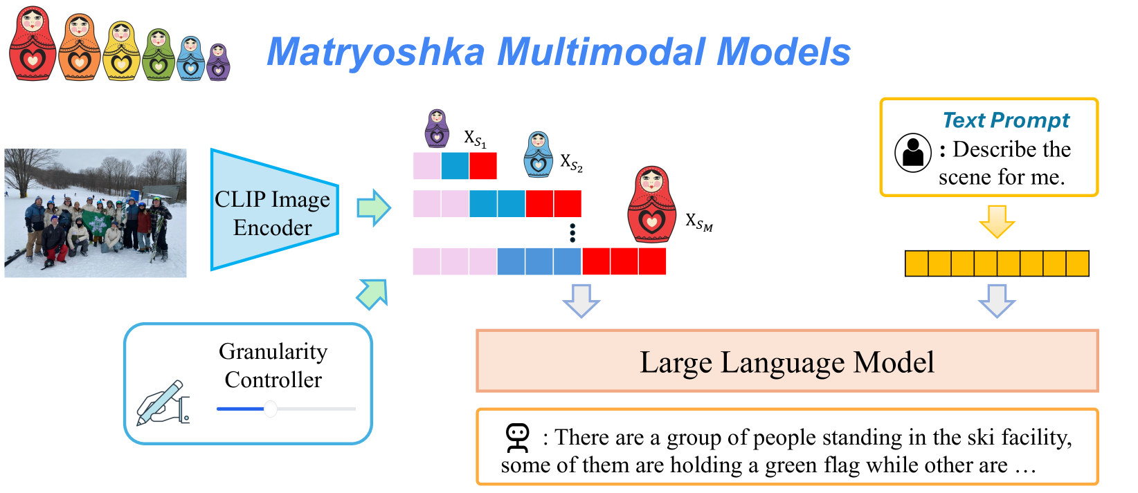</details> Figure 3: Architecture of our proposed Matryoshka Multimodal Models. The visual features from CLIP are represented as several groups of coarse-to-fine visual tokens. At test time, users can explicitly control the granularity of the visual features. Our goal is to learn a Large Multimodal Model (LMM) that represents visual content as nested sets of visual tokens capturing information across multiple coarse-to-fine granularities, so that one can explicitly control the visual granularity per test instance during inference. Here we introduce how we learn a Matryoshka doll-like token sequence. LMMs such as LLaVA [2] typically input a sequence of visual tokens as prefix tokens to the LLM for visual-linguistic reasoning. The visual encoder from pretrained vision-language models, such as CLIP [29] and SigLIP [46], is typically utilized to project the images into the set of visual tokens. In particular, the CLIP visual encoder represents an input image $I$ as an $H× W$ grid of visual tokens ${X}_H× W$ , where each $X_i∈ℝ^C$ is a $C$ dimensional feature vector. Our goal is to learn nested sets of visual tokens $[{X}_S_1,{X}_S_2,⋯,{X}_S_{M}]$ which encode the visual information in a coarse-to-fine manner. To this end, we enforce ${X}_S_{i}⊂{X}_S_{i+1},∀ i$ . Importantly, we do not introduce any new learnable parameters to the LMM. We instead optimize the CLIP visual encoder to learn the nested visual representation directly, and train the ensuing LLM to adapt to the learned nested set of tokens. For ease of exposition, we consider CLIP-ViT-L-336 [29] as the visual encoder, where an image is encoded as $24× 24$ visual tokens (576 total). We create $M$ sets of tokens e.g., $|S_i|∈\{1,9,36,144,576\}$ , in which the visual tokens at the coarser level are derived directly from those at the finer level. Specifically, given the initial $24× 24$ visual tokens, We sequentially apply $2× 2$ pooling with a stride 2, resulting in $12× 12,6× 6$ , and $3× 3$ visual tokens. Finally, we apply $3× 3$ pooling and get the most condensed single visual token. In this way, the sets of Matryoshka visual tokens can gradually preserve the spatial information in the original tokens while simultaneously forming a coarse-to-fine nested representation. We train M 3 by averaging the autoregressive next token prediction loss for each scale $S_i$ for each image $I_i$ . Specifically, given a Matryoshka visual representation ${X}_S_{i}$ for scale $S_i$ , we maximize the likelihood of the predicted tokens matching the ground-truth answer $X_a$ : $$ P(X_a\mid{X}_S_{i},X_q)=∏ _j=1^LP_\boldsymbol{θ}(x_j\mid{X}_S_{i},X_ q,X_a,<j), $$ where $\boldsymbol{θ}$ is the trainable parameters of the model, which includes both the CLIP visual encoder and the ensuing LLM. $X_q$ denotes the question in text format, $L$ denotes the token length of the ground truth answer $X_a$ , and $X_a,<j$ denotes all the ground truth answer tokens before the current prediction token $x_j$ , where $j$ denotes the token index during text token generation. We omit system messages for clarity, though they are part of the conditioning. Figure 3 shows our model architecture. The final objective averages over all $M$ visual token scales: $$ \min_\boldsymbol{θ}\frac{1}{M}∑_i=1^M-\log P(X_\mathrm {a}\mid{X}_S_{i},X_q). $$ With this objective function, M 3 learns nested sets of visual tokens that gradually include more details with increasing scale. For example, in Figure 1, the smaller set of visual tokens describes the whole scene at a high level while the larger set of visual tokens includes more details such as the Pepsi cup. Our training objective affords our model to conduct visual question answering under any granularity during inference. This can be particularly useful in resource constrained applications; e.g., the visual granularity can be flexibly adjusted based on the anticipated simplicity or complexity of the visual content while taking into account compute and memory constraints. ## 4 Experiments In this section, we first detail the experiment settings in Sec 4.1. Then we show the performance of M 3 on both image-level benchmarks 4.2 and video-level benchmarks 4.3. Finally, we analyze the behavior of Matryoshka Multimodal Models and provide ablations in Sec 4.4 and 4.5. ### 4.1 Experiment Settings #### Model We use LLaVA-1.5 [5] and LLaVA-NeXT [4] as the base LMMs, both with Vicuna 7B as the language model backbone. We finetune the whole model using the exact visual instruction data from LLaVA-1.5 and LLaVA-NeXT, respectively. The learning rate of LLM is $2× 10^-5$ and $1× 10^-5$ , respectively for LLaVA-1.5 and LLaVA-NeXT. The learning rate for the visual encoder is $2× 10^-5$ for both models. We train both models for 1 epoch using 8 NVIDIA H100 GPUs. Instead of training the language model from scratch, we initialize the language model weights from pre-trained LLaVA-1.5 and LLaVA-NeXT, which we empirically works better. We name our Matryoshka Multimodal Models LLaVA-1.5- M 3 and LLaVA-NeXT- M 3. #### Visual Token Scales We design 5 scales for the visual tokens. LLaVA-1.5 [5] and LLaVA-NeXT [4] both leverage CLIP-ViT-L-336 [29] as the visual encoder, where an image is embedded into $24× 24$ visual tokens. We gradually apply $2× 2$ pooling with stride 2, resulting in $12× 12,6× 6$ , and $3× 3$ visual tokens, where we finally apply a $3× 3$ pooling to get the final single visual token. Therefore, the size of Matryoshka visual token sets are $S∈\{1,9,36,144,576\}$ , following a nested manner. The efficiency anlaysis on the system level is shown in Appendix B, where M 3 boosts the speed of the LMM prefill process through diminished floating-point operations (FLOPs) and lessens computational memory requirements. #### Evaluations. For image understanding, we evaluate LLaVA-1.5 and LLaVA-NeXT on (a) diverse multimodal benchmarks: POPE [22], GQA [47], MMBench [23], VizWiz [48], SEEDBench [49], ScienceQA [50], MMMU [51], and (b) document understanding/Optical character recognition (OCR) benchmarks: DocVQA [52], ChartQA [25], AI2D [53] and TextVQA [24]. For video understanding, we use both (a) open ended video question answering benchmarks evaluated by GPT-3.5: MSVD-QA [54], MSRVTT-QA [54] and ActivityNet-QA [55]; and (b) multi-choice video question answering benchmarks: NExT-QA [56], IntentQA [57], and EgoSchema [58]. ### 4.2 Image Understanding #### LLaVA-1.5- M 3 We evaluate LLaVA-1.5- M 3 on the common multimodal understanding and reasoning benchmarks. Results are shown in Table 1. LLaVA-1.5- M 3 with full tokens maintains the performance of LLaVA-1.5 across diverse benchmarks. More importantly, our approach shows strong performance even with 1 or 9 tokens. Specifically, in MMBench, a comprehensive multimodal understanding benchmark, LLaVA-1.5- M 3 with 9 tokens surpasses Qwen-VL-Chat with 256 tokens, and achieves similar performance as Qwen-VL-Chat with even 1 token. Compared with InstructBLIP [59], LLaVA-1.5 M 3 with 9 tokens surpasses InstructBLIP-7B and InstructBLIP-13B across all benchmarks. This demonstrates that our model has both flexibility and strong empirical performance under diverse number of visual tokens. Table 1: Comparison between LLaVA-1.5- $M^3$ across various benchmarks under image understanding benchmarks. LLaVA-1.5- M 3 maintains the performance of LLaVA-1.5 while outperforming Qwen-VL and InstructBLIP with fewer tokens. Approach # Tokens MMBench GQA POPE VizWiz SEEDBench Qwen-VL [7] 256 38.2 59.3 - 35.2 56.3 Qwen-VL-Chat [7] 256 60.6 57.5 - 38.9 58.2 InstructBLIP-7B [59] 32 36.0 49.2 - 34.5 53.4 InstructBLIP-13B [59] 32 - 49.5 78.9 33.4 - LLaVA-1.5-7B [5] 576 64.8 62.0 85.9 54.4 60.5 LLaVA-1.5- $M^3$ 576 65.9 61.9 87.4 54.9 60.6 144 66.4 61.3 87.0 53.1 59.7 36 64.8 60.3 85.5 52.8 58.0 9 63.1 58.0 83.4 51.9 55.4 1 59.5 52.6 78.4 49.4 50.1 #### LLaVA-NeXT- M 3 We use the proposed Matryoshka Multimodal Models to finetune LLaVA-NeXT, and compare LLaVA-NeXT- M 3 with SS, which denotes the setting where the LLaVA-NeXT is trained under a S pecific S cale of visual tokens also for 1 epoch. We also include the oracle upperbound performance. Specifically, ‘Oracle’ denotes the case where the best tradeoff between visual tokens and performance is picked for each test instance. Specifically, for each test instance, we select the the scale with the fewest amount of tokens but can answer the question correctly. Results are shown in Table 2. Our approach, M 3, is at least as good as SS, while performing better on tasks such as document understanding (TextVQA and ChartQA) and common benchmarks such as MMBench [23]. Table 2: Comparison of approaches with the SS baseline and $M^3$ across various benchmarks under LLaVA-NeXT [4]. Here # Tokens denotes the number of visual tokens per image grid in LLaVA-NeXT. SS denotes the baseline model trained with a S pecific S cale of visual tokens. M 3 is at least as good as SS, while performing better on tasks such as TextVQA, ChartQA, and MMBench. Oracle denotes the case where the best tradeoff between visual tokens and performance is picked. # Tokens Per Grid Approach TextVQA AI2D ChartQA DocVQA MMBench POPE ScienceQA MMMU 576 SS 64.53 64.83 59.28 75.40 66.58 87.02 72.29 34.3 $M^3$ 63.13 66.71 58.96 72.61 67.96 87.20 72.46 34.0 144 SS 62.16 65.77 55.28 67.69 67.78 87.66 72.15 36.4 $M^3$ 62.61 68.07 57.04 66.48 69.50 87.67 72.32 36.1 36 SS 58.15 65.90 45.40 56.89 67.01 86.75 71.87 36.2 $M^3$ 58.71 67.36 50.24 55.94 68.56 87.29 72.11 36.8 9 SS 50.95 65.06 37.76 44.21 65.29 85.62 72.37 36.8 $M^3$ 51.97 66.77 42.00 43.52 67.35 86.17 71.85 35.2 1 SS 38.39 63.76 28.96 33.11 61.43 82.83 72.32 35.3 $M^3$ 38.92 64.57 31.04 31.63 62.97 83.38 71.19 34.8 Oracle # Tokens 31.39 11.54 41.78 64.09 8.90 6.08 7.43 22.85 Performance 70.51 76.36 70.76 81.73 74.35 94.29 76.07 50.44 Our results also show that dataset level biases towards the visual token scales do exist. For example, ScienceQA maintains consistent performance across all visual token scales. AI2D and MMBench only encounter a small performance drop for even as few as 9 to 1 tokens. On the other hand, dense visual perception tasks such as TextVQA and DocVQA show a significant performance drop with fewer tokens. This analysis shows that M 3 could serve as a framework to analyze the granularity that a benchmark needs. Furthermore, there is a large gap between the model’s actual performance under full tokens and the upper-bound oracle. This indicates that using full tokens cannot always result in the optimal performance for all samples; i.e., there is a large room of improvement towards the oracle point. ### 4.3 Video Understanding Following IG-VLM [60], we directly conduct zero-shot inference on diverse video benchmarks using LLaVA-NeXT- M 3. Specifically, 6 frames are uniformly sampled over the entire video, then arranged as a collage, which is fed into LLaVA-NeXT along with the question to get the response. Results under LLaVA-NeXT- M 3 and recent video LMMs are show in Table 3. LLaVA-NeXT- M 3 with full visual tokens again shows comparable performance with LLaVA-NeXT. More interestingly, results indicate that full visual tokens usually do not lead to the best performance in video understanding tasks. Specifically, on 4 out of 6 benchmarks, full visual tokens show less desirable performance compared to 720 or 180 visual tokens. We suspect that very long visual context could bring distraction (e.g., too much focus on potentially irrelevant background) to the model’s prediction, where a compact representation of the video focusing on the more relevant information may be more advantageous. Finally, for most video understanding tasks such as ActivityNet, IntentQA and EgoSchema, with 9 tokens per image grid (45 tokens in total), the accuracy difference compared to full tokens (2880 in total) is less than 1%. This demonstrates that the video questions in these benchmarks usually require very sparse visual information, as the source of such video understanding benchmarks mostly comes from natural scenes, which matches our observation in image understanding benchmarks. Table 3: Overall accuracy of LLaVA-NeXT- M 3 and recent video LMMs on various video understanding benchmarks. Here # Tokens denotes the overall number of visual tokens across all frames. Approach # Tokens MSVD MSRVTT ActivityNet NextQA IntentQA EgoSchema Video-LLaMA [61] - 51.6 29.6 12.4 - - - LLaMA-Adapter [62] - 54.9 43.8 34.2 - - - Video-ChatGPT [63] - 64.9 49.3 35.2 - - - Video-LLaVA [64] 2048 70.7 59.2 45.3 - - - InternVideo [65] - - - - 59.1 - 32.1 LLaVA-NeXT-7B [4] 2880 78.8 63.7 54.3 63.1 60.3 35.8 LLaVA-NeXT-7B- M 3 2880 78.2 64.5 53.9 63.1 58.8 36.8 720 79.0 64.5 55.0 62.6 59.6 37.2 180 77.9 63.7 55.0 61.4 59.3 37.6 45 75.8 63.0 53.2 59.5 58.7 38.8 5 73.5 62.7 50.8 56.5 56.7 36.2 ### 4.4 In-depth Analysis #### M 3 shows much stronger performance compared to heuristics based sampling at test time. 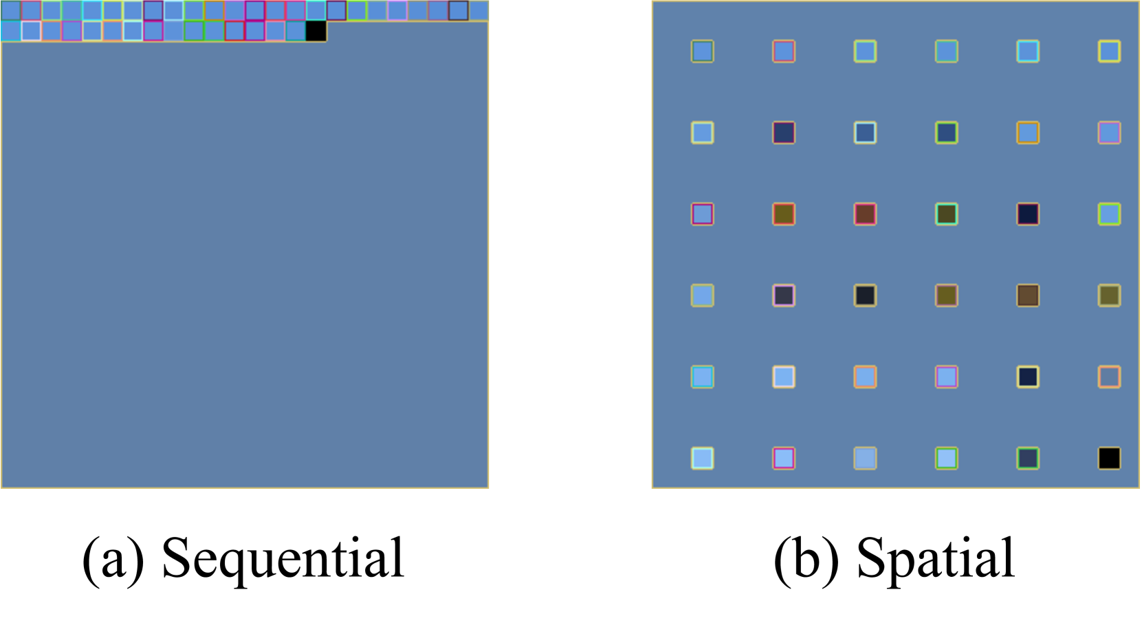A simple way to reduce the number of visual tokens via a training-free way is to conduct heuristic token merging or reduction. In Table 4, we compare M 3 with three training-free approaches: average pooling, spatial sampling, and sequential sampling. M 3 is much more resilient when the number of tokens decreases, while the heuristic based sampling approaches show dramatic performance drop. A visualization of the spatial and sequential sampling is shown in Figure 5. Table 4: Comparison between M 3, and heuristics based sampling baselines—average pooling, spatial sampling, and sequential sampling—at inference time on MMBench with the LLaVA-NeXT architecture. # Tokens M 3 Average Pooling Spatial Sampling Sequential Sampling 576 67.96 67.18 67.18 67.18 144 69.50 61.68 65.81 60.14 36 68.56 50.77 60.05 44.76 9 67.35 45.45 45.45 31.96 1 62.97 19.33 26.29 22.42 #### M 3 serves as a good metric for image complexity. 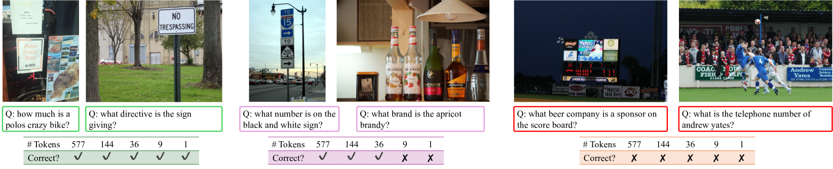We extract the response from LLaVA-NeXT- M 3 in the TextVQA benchmark, and show the samples where using visual tokens across different scales can answer the question correctly and incorrectly. Shown in Figure 4, the OCR performance aligns with the complexity of the images, which indicates that M 3 can be utilized as a metric towards sample level complexity. <details> <summary>x3.png Details</summary>  ### Visual Description ## Visual Question Answering (VQA) Performance Comparison ### Overview The image is a composite figure displaying six distinct visual question-answering (VQA) scenarios. Each scenario is presented in a separate panel, arranged horizontally. Each panel contains: 1) a photograph, 2) a specific question about the photograph, and 3) a small table showing the performance of five different models or methods, measured by token count and correctness. The panels are grouped by colored borders (green, purple, red), likely indicating different performance tiers or categories. ### Components/Axes The image is segmented into six vertical panels. Each panel has the following consistent structure: 1. **Photograph**: A real-world image containing visual information relevant to the question. 2. **Question Box**: A colored box (green, purple, or red) containing a question prefixed with "Q:". 3. **Performance Table**: A small table with two rows: * **# Tokens**: Lists five numerical values (577, 144, 36, 9, 1), presumably representing the token count or model size for five different systems. * **Correct?**: Shows a checkmark (✓) or cross (✗) for each token count, indicating whether the answer generated by that system was correct. **Spatial Grounding**: The legend (the performance table) is consistently placed at the bottom of each panel. The question is positioned directly below the photograph. The colored borders group the panels: the first two are green, the next two are purple, and the final two are red. ### Detailed Analysis **Panel 1 (Green Border - Leftmost)** * **Photograph**: A close-up of a storefront or kiosk. A prominent sign reads "Polos Crazy Bike" with a price of "$20.00" below it. Other text and images are partially visible but less clear. * **Question**: "Q: how much is a polos crazy bike?" * **Performance Table**: * # Tokens: 577, 144, 36, 9, 1 * Correct?: ✓, ✓, ✓, ✓, ✓ * **Trend**: All five models, regardless of token count, answered correctly. **Panel 2 (Green Border)** * **Photograph**: A "NO TRESPASSING" sign on a metal post in a grassy area with trees and a building in the background. * **Question**: "Q: what directive is the sign giving?" * **Performance Table**: * # Tokens: 577, 144, 36, 9, 1 * Correct?: ✓, ✓, ✓, ✓, ✓ * **Trend**: All five models answered correctly. **Panel 3 (Purple Border)** * **Photograph**: A street scene with a black and white directional sign on a lamppost. The sign has arrows and numbers. The top section shows "TO 15" with an arrow pointing up. The bottom section shows "TO 201" with an arrow pointing right. * **Question**: "Q: what number is on the black and white sign?" * **Performance Table**: * # Tokens: 577, 144, 36, 9, 1 * Correct?: ✓, ✓, ✓, ✗, ✗ * **Trend**: The three larger models (577, 144, 36 tokens) answered correctly. The two smallest models (9 and 1 token) failed. **Panel 4 (Purple Border)** * **Photograph**: A collection of bottles on a shelf. One bottle in the center has a label that reads "MONIN" and "Abricot" (French for Apricot). Other bottles include "Stolichnaya" vodka and "Grand Marnier". * **Question**: "Q: what brand is the apricot brandy?" * **Performance Table**: * # Tokens: 577, 144, 36, 9, 1 * Correct?: ✓, ✓, ✓, ✗, ✗ * **Trend**: Identical to Panel 3. The three larger models succeeded; the two smallest failed. **Panel 5 (Red Border)** * **Photograph**: A baseball scoreboard at night. The scoreboard displays team logos and names. A prominent sponsor logo for "Budweiser" (the beer company) is visible at the top. * **Question**: "Q: what beer company is a sponsor on the score board?" * **Performance Table**: * # Tokens: 577, 144, 36, 9, 1 * Correct?: ✗, ✗, ✗, ✗, ✗ * **Trend**: All five models failed to answer correctly. **Panel 6 (Red Border - Rightmost)** * **Photograph**: A soccer match scene. In the background, an advertising board is visible with the text "Andrew Yates" and a telephone number "01283 740501". * **Question**: "Q: what is the telephone number of andrew yates?" * **Performance Table**: * # Tokens: 577, 144, 36, 9, 1 * Correct?: ✗, ✗, ✗, ✗, ✗ * **Trend**: All five models failed to answer correctly. ### Key Observations 1. **Performance Gradient by Task Difficulty**: The colored borders correlate with overall success rate. Green panels (easy tasks) have 100% success across all models. Purple panels (medium difficulty) show a clear performance cliff: models with 36+ tokens succeed, while those with 9 or fewer fail. Red panels (hard tasks) result in complete failure for all models. 2. **Token Count vs. Capability**: There is a strong, but not absolute, correlation between token count (model size) and performance. Larger models (577, 144, 36 tokens) handle the medium-difficulty tasks, while all models struggle with the hard tasks. 3. **Nature of Failures**: The failures in the red panels are not due to model size but likely due to the inherent difficulty of the tasks. Panel 5 requires identifying a specific brand logo in a cluttered scene, and Panel 6 requires precise optical character recognition (OCR) of a small, non-central text element in a complex image. 4. **Task Types**: The questions test different capabilities: simple text reading (Panel 1), sign interpretation (Panel 2), selective number extraction from multiple options (Panel 3), brand identification from a label (Panel 4), logo recognition (Panel 5), and fine-grained OCR (Panel 6). ### Interpretation This figure demonstrates a benchmark for evaluating multimodal AI models on visual question answering. The data suggests a clear hierarchy of task difficulty for current models. * **Foundational Tasks (Green)**: Reading prominent, isolated text and understanding simple symbolic signs are solved problems, even for very small models (1 token). * **Intermediate Tasks (Purple)**: Selecting the correct information from a visually cluttered scene with multiple similar elements (e.g., choosing between numbers 15 and 201 on a sign, or identifying the correct brand among several bottles) requires a moderate level of model capacity. There is a sharp performance drop below a certain model size threshold (somewhere between 36 and 9 tokens in this evaluation). * **Advanced Tasks (Red)**: Recognizing specific commercial logos in context and performing high-precision OCR on small, incidental text in complex scenes remain significant challenges for all models tested, regardless of size. This indicates a gap in current capabilities for fine-grained visual understanding and text extraction in unconstrained environments. The figure effectively argues that while scaling model size (tokens) improves performance on tasks of moderate complexity, it does not guarantee success on all visual understanding problems. Some tasks require specific architectural strengths or training data that even larger models in this set lack. The consistent failure on the red-panel tasks highlights a frontier for future model development. </details> Figure 4: TextVQA test samples with correct and incorrect predictions upon different scales. Answers vary with different number of visual tokens. In addition, M 3 can serve as a framework to evaluate the complexity of images. #### Large gap between oracle and actual performance. As shown in Table 2, the oracle upper-bound can use very few ( $6∼ 64$ ) tokens yet achieve at least 10% better performance compared to full visual tokens. This suggests that a visual token scale predictor, where the model learns to automatically select the best visual token scale given the input images or both input images and questions, has potential to achieve a better tradeoff. This would be interesting future work. #### Zero-shot generalization to longer visual sequences. Here we extend the length of the visual tokens at inference time to study the model’s zero-shot generalization behavior. Results under LLaVA-NeXT are shown in Table 5. Here LLaVA-NeXT- M 3 is trained on $2× 2$ image grids but evaluated on $3× 3$ grids. We set the number of visual tokens to be 144 in each image during evaluation. The model obtains a significant improvement in document understanding by 2.12, 1.80, and 4.11 on TextVQA, ChartQA, and DocVQA, respectively, while maintaining the same performance on benchmarks mainly composed of natural scene images. $3× 3$ image grids with 144 tokens per grid own 1440 tokens, yet achieve similar performance with the default LLaVA-NeXT $2× 2$ image grids with 2880 total tokens (576 tokens per grid). This indicates it is promising to feed more subimages while making the number of visual tokens within each subimage much smaller. Table 5: Performance comparison of different image grid configurations with LLaVA-NeXT- M 3. # Grids # Tokens per grid Overall # Tokens TextVQA AI2D ChartQA DocVQA MMBench POPE ScienceQA $2× 2$ 144 720 62.61 68.07 57.04 66.48 69.50 87.67 72.32 $3× 3$ 144 1440 64.73 67.75 58.84 70.59 69.50 87.67 72.22 $2× 2$ 576 2880 63.13 66.71 58.96 72.61 67.96 87.20 72.46 <details> <summary>x4.png Details</summary>  ### Visual Description ## Diagram: Sequential vs. Spatial Data Representation ### Overview The image displays two side-by-side diagrams illustrating different methods of organizing or representing data elements. The left diagram is labeled "(a) Sequential" and the right is labeled "(b) Spatial". Both diagrams use a consistent visual language of small squares with colored borders and varying fill colors against a uniform blue-gray background. ### Components/Axes * **Labels:** The primary textual labels are located below each diagram: * Left: `(a) Sequential` * Right: `(b) Spatial` * **Visual Elements:** Both diagrams consist of a large, solid blue-gray square field containing smaller squares. * **Diagram (a) Sequential:** Contains a single horizontal row of small squares positioned at the very top edge of the main field. * **Diagram (b) Spatial:** Contains a 6x6 grid of small squares, evenly distributed across the entire main field. ### Detailed Analysis **Diagram (a) Sequential:** * **Structure:** A single, linear sequence of 24 small squares arranged in one row at the top of the frame. * **Element Details:** Each small square has a distinct colored border. The fill colors are mostly light blue, with one solid black square. * **Spatial Grounding:** The row is anchored to the top-left corner and extends horizontally to the right. The black square is the 12th element from the left. * **Border Colors (approximate, from left to right):** The sequence includes borders in shades of cyan, magenta, green, orange, blue, and purple. The pattern does not appear to follow a simple repeating order. **Diagram (b) Spatial:** * **Structure:** A regular 6x6 grid (36 total squares) with even spacing between rows and columns. * **Element Details:** Each small square has a colored border and a distinct fill color. Fill colors include various shades of blue, brown, olive green, gray, and black. * **Spatial Grounding:** The grid fills the entire square field. The black-filled square is located in the bottom-right corner (row 6, column 6). * **Color Distribution:** There is no immediately obvious pattern to the fill or border colors based on grid position. Colors appear distributed without a clear gradient or grouping. ### Key Observations 1. **Fundamental Contrast:** The core difference is organizational. Diagram (a) shows elements in a strict, one-dimensional order (a sequence). Diagram (b) shows elements in a two-dimensional arrangement (a spatial field). 2. **Element Count:** The sequential diagram contains 24 elements in a line. The spatial diagram contains 36 elements in a grid. 3. **The Black Square:** Both diagrams contain exactly one solid black square. In the sequential diagram, it is embedded within the line. In the spatial diagram, it occupies the final grid position (bottom-right). 4. **Color Complexity:** The spatial diagram exhibits a wider variety of fill colors compared to the sequential diagram, which uses a more uniform light blue fill with varied borders. ### Interpretation This image is a conceptual diagram contrasting two fundamental paradigms for data organization or memory addressing. * **Sequential (a):** Represents data stored or accessed in a linear, ordered list. This is analogous to a tape, a queue, or a simple array where position is defined by an index (e.g., 1st, 2nd, 3rd...). The single row emphasizes order and progression. The black square could represent a specific data point, a marker, or the current position in the sequence. * **Spatial (b):** Represents data distributed across a two-dimensional space, like a matrix, a pixel grid, or a map. Position is defined by coordinates (e.g., row, column). This model is essential for images, geographical data, and any context where relationships are defined by proximity in a plane. The black square here denotes a specific coordinate location. The diagrams likely serve to explain concepts in computer science (memory layout, data structures), cognitive science (how information is mentally organized), or visualization theory. The choice between a sequential or spatial representation has profound implications for how data is processed, searched, and understood. The sequential model prioritizes order and sequence, while the spatial model prioritizes location and relational proximity. </details> Figure 5: Visualization of sequential and spatial sampling. Given $24× 24$ girds, the visualized cells denote the sampled tokens. ### 4.5 Ablation Studies We ablate the key designs in M 3, including the sampling method of Matryoshka visual tokens, and training strategy. #### Matryoshka visual token sampling. Here we compare three different ways to select the visual tokens for Matryoshka Multimodal Models, including average pooling, spatial sampling, and sequential sampling, which is illustrated in Figure 5. Shown in Table 6, averaging pooling shows better performance than the two alternatives across diverse benchmarks. In general, sequential sampling performs the worst. We hypothesize that this is due to the visual tokens having spatial information, while sequential sampling does not naturally align with the spatial distribution of the visual tokens. Table 6: Ablation on Matryoshka visual token sampling including average pooling, sequential sampling, and spatial sampling. TextVQA MMBench AI2D Num of Vis Tokens Avg Pooling Sequential Spatial Avg Pooling Sequential Spatial Avg Pooling Sequential Spatial 576 63.13 59.37 60.45 67.96 64.60 64.43 66.71 65.61 64.96 144 62.61 55.80 58.33 69.50 64.18 64.52 68.07 64.90 64.96 36 58.71 52.79 52.39 68.56 63.92 64.69 67.36 64.51 64.02 9 51.97 44.05 44.19 67.35 63.14 62.11 66.77 63.70 63.92 1 38.92 28.03 29.91 62.97 59.36 57.47 64.57 63.21 63.08 Table 7: Performance comparison of training LLaVA-NeXT- M 3 with and without training the LLM across diverse benchmarks. We see a clear drop when freezing the LLM. Num of Vis Tokens TextVQA MMBench AI2D DocVQA w/ LLM w/o LLM w/ LLM w/o LLM w/ LLM w/o LLM w/ LLM w/o LLM 576 63.13 61.16 67.96 63.66 66.71 63.92 72.61 69.15 144 62.61 57.79 69.50 65.21 68.07 63.73 66.48 59.77 36 58.71 49.75 68.56 63.92 67.36 62.89 55.94 44.08 9 51.97 36.15 67.35 61.08 66.77 62.05 43.52 28.36 1 38.92 19.72 62.97 51.80 64.57 60.59 31.63 17.37 Table 8: Impact of (a) initializing the LLM weights from LLaVA, and (b) averaging the loss from all scales vs randomly selecting a scale for each sample during training. Technique TextVQA AI2D Init LLM weights from LLaVA ✓ ✓ ✓ ✓ Average losses over all scales ✓ ✓ ✓ ✓ 576 60.36 62.25 61.01 63.13 62.40 65.06 65.84 66.71 144 59.61 61.02 59.80 62.61 63.67 65.61 65.77 68.07 36 54.86 55.91 55.32 58.71 63.67 65.32 66.68 67.36 9 46.84 47.04 48.80 51.97 63.02 64.83 65.38 66.77 1 33.78 33.68 36.05 38.92 61.53 63.21 63.37 64.57 #### Training the entire LMM vs only training CLIP. Since the nested behavior of Matryoshka visual tokens is learned within the CLIP visual encoder, we next evaluate whether it is necessary to also finetune the LLM. Shown in Table 7, training the whole LLM achieves better performance. This demonstrates that by also training the LLM, the model can better adapt to the patterns of the visual tokens distributed in the Matryoshka manner. As explained in Sec. 3 and 4.1, we (a) initialize the LLM weights from LLaVA and (b) minimize the loss averaged upon all visual token scales for each sample during training. An alternative choice is to randomly sample a visual token scale. Shown in Table 8, initializing the LLM weights from LLaVA and minimizing the losses over all scales shows consistent performance boost compared to using the vanilla text-only pre-trained LLM weights [8] and randomly selecting a visual token scale. Initializing the LLM weights from LLaVA makes the training process of M 3 more stable. By learning all scales at once, the model is forced to learn the nested behavior for each sample, which leads to better performance. ## 5 Conclusion and Future Work We introduced M 3: Matryoshka Multimodal Models, which learns to represent visual content as nested sets of visual tokens, capturing information across multiple coarse-to-fine granularities. LMMs equipped with M 3 afford explicit control over the visual granularity per test instance during inference. We also showed that M 3 can serve as an analysis framework to investigate the visual granularity needed for existing datasets, where we discovered that a large number of multimodal benchmarks only need as few as 9 visual tokens to obtain accuracy similar to that of using all visual tokens, especially for video understanding. Furthermore, we disclosed a large performance-efficiency gap between the oracle upper-bound and the model’s performance. Our work can be naturally extended to other domains. For example, the long context in a text-only LLM or vision tokens in dense vision tasks can also be represented as nested sets of tokens in a Matryoshka manner. One limitation of our current approach is that we are lacking an effective visual token predictor that can bridge the gap between the oracle and LMM’s actual performance at a specific scale. We believe this would be an exciting next direction of research in this space. ## Acknowledgement This work was supported in part by NSF CAREER IIS2150012, and Institute of Information & communications Technology Planning & Evaluation(IITP) grants funded by the Korea government(MSIT) (No. 2022-0-00871, Development of AI Autonomy and Knowledge Enhancement for AI Agent Collaboration) and (No. RS2022-00187238, Development of Large Korean Language Model Technology for Efficient Pre-training), and Microsoft Accelerate Foundation Models Research Program. ## References - [1] OpenAI. Gpt-4v(ision) system card. https://cdn.openai.com/papers/GPTV_System_Card.pdf, 2023. - [2] Haotian Liu, Chunyuan Li, Qingyang Wu, and Yong Jae Lee. Visual instruction tuning. NeurIPS, 2023. - [3] Deyao Zhu, Jun Chen, Xiaoqian Shen, Xiang Li, and Mohamed Elhoseiny. Minigpt-4: Enhancing vision-language understanding with advanced large language models. ICLR, 2024. - [4] Haotian Liu, Chunyuan Li, Yuheng Li, Bo Li, Yuanhan Zhang, Sheng Shen, and Yong Jae Lee. Llava-next: Improved reasoning, ocr, and world knowledge, January 2024. - [5] Haotian Liu, Chunyuan Li, Yuheng Li, and Yong Jae Lee. Improved baselines with visual instruction tuning, 2024. - [6] Weihan Wang, Qingsong Lv, Wenmeng Yu, Wenyi Hong, Ji Qi, Yan Wang, Junhui Ji, Zhuoyi Yang, Lei Zhao, Xixuan Song, Jiazheng Xu, Bin Xu, Juanzi Li, Yuxiao Dong, Ming Ding, and Jie Tang. Cogvlm: Visual expert for pretrained language models, 2023. - [7] Jinze Bai, Shuai Bai, Shusheng Yang, Shijie Wang, Sinan Tan, Peng Wang, Junyang Lin, Chang Zhou, and Jingren Zhou. Qwen-vl: A versatile vision-language model for understanding, localization, text reading, and beyond. arXiv preprint arXiv:2308.12966, 2023. - [8] Vicuna. Vicuna: An open-source chatbot impressing gpt-4 with 90%* chatgpt quality. https://vicuna.lmsys.org/, 2023. - [9] Meta. Llama-3. https://ai.meta.com/blog/meta-llama-3/, 2024. - [10] Bin Lin, Bin Zhu, Yang Ye, Munan Ning, Peng Jin, and Li Yuan. Video-llava: Learning united visual representation by alignment before projection. arXiv preprint arXiv:2311.10122, 2023. - [11] Hang Zhang, Xin Li, and Lidong Bing. Video-llama: An instruction-tuned audio-visual language model for video understanding. arXiv preprint arXiv:2306.02858, 2023. - [12] Yuanhan Zhang, Bo Li, haotian Liu, Yong jae Lee, Liangke Gui, Di Fu, Jiashi Feng, Ziwei Liu, and Chunyuan Li. Llava-next: A strong zero-shot video understanding model, April 2024. - [13] Gemini Team. Gemini: A family of highly capable multimodal models, 2024. - [14] Daniel Bolya, Cheng-Yang Fu, Xiaoliang Dai, Peizhao Zhang, Christoph Feichtenhofer, and Judy Hoffman. Token merging: Your ViT but faster. In International Conference on Learning Representations, 2023. - [15] Liang Chen, Haozhe Zhao, Tianyu Liu, Shuai Bai, Junyang Lin, Chang Zhou, and Baobao Chang. An image is worth 1/2 tokens after layer 2: Plug-and-play inference acceleration for large vision-language models. arXiv preprint arXiv:2403.06764, 2024. - [16] Yuzhang Shang, Mu Cai, Bingxin Xu, Yong Jae Lee, and Yan Yan. Llava-prumerge: Adaptive token reduction for efficient large multimodal models. arXiv preprint arXiv:2403.15388, 2024. - [17] Tsung-Yi Lin, Michael Maire, Serge Belongie, James Hays, Pietro Perona, Deva Ramanan, Piotr Dollár, and C Lawrence Zitnick. Microsoft coco: Common objects in context. In Computer Vision–ECCV 2014: 13th European Conference, Zurich, Switzerland, September 6-12, 2014, Proceedings, Part V 13, pages 740–755. Springer, 2014. - [18] Mike G Harris and Christos D Giachritsis. Coarse-grained information dominates fine-grained information in judgments of time-to-contact from retinal flow. Vision research, 40(6):601–611, 2000. - [19] Jay Hegdé. Time course of visual perception: coarse-to-fine processing and beyond. Progress in neurobiology, 84(4):405–439, 2008. - [20] Aditya Kusupati, Gantavya Bhatt, Aniket Rege, Matthew Wallingford, Aditya Sinha, Vivek Ramanujan, William Howard-Snyder, Kaifeng Chen, Sham Kakade, Prateek Jain, et al. Matryoshka representation learning. Advances in Neural Information Processing Systems, 35:30233–30249, 2022. - [21] Yash Goyal, Tejas Khot, Douglas Summers-Stay, Dhruv Batra, and Devi Parikh. Making the v in vqa matter: Elevating the role of image understanding in visual question answering. In Proceedings of the IEEE conference on computer vision and pattern recognition, pages 6904–6913, 2017. - [22] Yifan Li, Yifan Du, Kun Zhou, Jinpeng Wang, Wayne Xin Zhao, and Ji-Rong Wen. Evaluating object hallucination in large vision-language models. arXiv preprint arXiv:2305.10355, 2023. - [23] Yuan Liu, Haodong Duan, Yuanhan Zhang, Bo Li, Songyang Zhang, Wangbo Zhao, Yike Yuan, Jiaqi Wang, Conghui He, Ziwei Liu, et al. Mmbench: Is your multi-modal model an all-around player? arXiv preprint arXiv:2307.06281, 2023. - [24] Amanpreet Singh, Vivek Natarajan, Meet Shah, Yu Jiang, Xinlei Chen, Dhruv Batra, Devi Parikh, and Marcus Rohrbach. Towards vqa models that can read. In Proceedings of the IEEE/CVF conference on computer vision and pattern recognition, pages 8317–8326, 2019. - [25] Ahmed Masry, Do Long, Jia Qing Tan, Shafiq Joty, and Enamul Hoque. ChartQA: A benchmark for question answering about charts with visual and logical reasoning. In Findings of the Association for Computational Linguistics: ACL 2022, pages 2263–2279, Dublin, Ireland, May 2022. Association for Computational Linguistics. - [26] OpenAI. Chatgpt. https://openai.com/blog/chatgpt/, 2023. - [27] OpenAI. Gpt-4 technical report. 2023. - [28] Hugo Touvron, Thibaut Lavril, Gautier Izacard, Xavier Martinet, Marie-Anne Lachaux, Timothée Lacroix, Baptiste Rozière, Naman Goyal, Eric Hambro, Faisal Azhar, et al. Llama: Open and efficient foundation language models. arXiv preprint arXiv:2302.13971, 2023. - [29] Alec Radford, Jong Wook Kim, Chris Hallacy, Aditya Ramesh, Gabriel Goh, Sandhini Agarwal, Girish Sastry, Amanda Askell, Pamela Mishkin, Jack Clark, et al. Learning transferable visual models from natural language supervision. In International conference on machine learning, pages 8748–8763. PMLR, 2021. - [30] Mu Cai, Haotian Liu, Siva Karthik Mustikovela, Gregory P. Meyer, Yuning Chai, Dennis Park, and Yong Jae Lee. Making large multimodal models understand arbitrary visual prompts. In IEEE Conference on Computer Vision and Pattern Recognition, 2024. - [31] Shilong Zhang, Peize Sun, Shoufa Chen, Min Xiao, Wenqi Shao, Wenwei Zhang, Kai Chen, and Ping Luo. Gpt4roi: Instruction tuning large language model on region-of-interest. arXiv preprint arXiv:2307.03601, 2023. - [32] Keqin Chen, Zhao Zhang, Weili Zeng, Richong Zhang, Feng Zhu, and Rui Zhao. Shikra: Unleashing multimodal llm’s referential dialogue magic. arXiv preprint arXiv:2306.15195, 2023. - [33] Zhiliang Peng, Wenhui Wang, Li Dong, Yaru Hao, Shaohan Huang, Shuming Ma, and Furu Wei. Kosmos-2: Grounding multimodal large language models to the world. arXiv preprint arXiv:2306.14824, 2023. - [34] Hao Zhang, Hongyang Li, Feng Li, Tianhe Ren, Xueyan Zou, Shilong Liu, Shijia Huang, Jianfeng Gao, Lei Zhang, Chunyuan Li, and Jianwei Yang. Llava-grounding: Grounded visual chat with large multimodal models, 2023. - [35] Yining Hong, Haoyu Zhen, Peihao Chen, Shuhong Zheng, Yilun Du, Zhenfang Chen, and Chuang Gan. 3d-llm: Injecting the 3d world into large language models. NeurIPS, 2023. - [36] Kaiming He, Xiangyu Zhang, Shaoqing Ren, and Jian Sun. Deep residual learning for image recognition. In CVPR, 2016. - [37] Alexey Dosovitskiy, Lucas Beyer, Alexander Kolesnikov, Dirk Weissenborn, Xiaohua Zhai, Thomas Unterthiner, Mostafa Dehghani, Matthias Minderer, Georg Heigold, Sylvain Gelly, Jakob Uszkoreit, and Neil Houlsby. An image is worth 16x16 words: Transformers for image recognition at scale. ICLR, 2021. - [38] Chao Jia, Yinfei Yang, Ye Xia, Yi-Ting Chen, Zarana Parekh, Hieu Pham, Quoc Le, Yun-Hsuan Sung, Zhen Li, and Tom Duerig. Scaling up visual and vision-language representation learning with noisy text supervision. In International conference on machine learning, pages 4904–4916. PMLR, 2021. - [39] Jacob Devlin, Ming-Wei Chang, Kenton Lee, and Kristina Toutanova. Bert: Pre-training of deep bidirectional transformers for language understanding. arXiv preprint arXiv:1810.04805, 2018. - [40] Xianming Li, Zongxi Li, Jing Li, Haoran Xie, and Qing Li. 2d matryoshka sentence embeddings. arXiv preprint arXiv:2402.14776, 2024. - [41] Ashish Vaswani, Noam Shazeer, Niki Parmar, Jakob Uszkoreit, Llion Jones, Aidan N Gomez, Łukasz Kaiser, and Illia Polosukhin. Attention is all you need. In Advances in Neural Information Processing Systems, pages 5998–6008, 2017. - [42] Sinong Wang, Belinda Z. Li, Madian Khabsa, Han Fang, and Hao Ma. Linformer: Self-attention with linear complexity, 2020. - [43] Nikita Kitaev, Lukasz Kaiser, and Anselm Levskaya. Reformer: The efficient transformer. In International Conference on Learning Representations, 2020. - [44] Joakim Bruslund Haurum, Sergio Escalera, Graham W. Taylor, and Thomas B. Moeslund. Which tokens to use? investigating token reduction in vision transformers. In Proceedings of the IEEE/CVF International Conference on Computer Vision (ICCV) Workshops, October 2023. - [45] Wenbo Hu, Zi-Yi Dou, Liunian Harold Li, Amita Kamath, Nanyun Peng, and Kai-Wei Chang. Matryoshka query transformer for large vision-language models. arXiv preprint arXiv:2405.19315, 2024. - [46] Xiaohua Zhai, Basil Mustafa, Alexander Kolesnikov, and Lucas Beyer. Sigmoid loss for language image pre-training. In Proceedings of the IEEE/CVF International Conference on Computer Vision, pages 11975–11986, 2023. - [47] Drew A Hudson and Christopher D Manning. Gqa: A new dataset for real-world visual reasoning and compositional question answering. In CVPR, 2019. - [48] Danna Gurari, Qing Li, Abigale J Stangl, Anhong Guo, Chi Lin, Kristen Grauman, Jiebo Luo, and Jeffrey P Bigham. Vizwiz grand challenge: Answering visual questions from blind people. In Proceedings of the IEEE conference on computer vision and pattern recognition, pages 3608–3617, 2018. - [49] Bohao Li, Rui Wang, Guangzhi Wang, Yuying Ge, Yixiao Ge, and Ying Shan. Seed-bench: Benchmarking multimodal llms with generative comprehension. arXiv preprint arXiv:2307.16125, 2023. - [50] Pan Lu, Swaroop Mishra, Tanglin Xia, Liang Qiu, Kai-Wei Chang, Song-Chun Zhu, Oyvind Tafjord, Peter Clark, and Ashwin Kalyan. Learn to explain: Multimodal reasoning via thought chains for science question answering. Advances in Neural Information Processing Systems, 2022. - [51] Xiang Yue, Yuansheng Ni, Kai Zhang, Tianyu Zheng, Ruoqi Liu, Ge Zhang, Samuel Stevens, Dongfu Jiang, Weiming Ren, Yuxuan Sun, Cong Wei, Botao Yu, Ruibin Yuan, Renliang Sun, Ming Yin, Boyuan Zheng, Zhenzhu Yang, Yibo Liu, Wenhao Huang, Huan Sun, Yu Su, and Wenhu Chen. Mmmu: A massive multi-discipline multimodal understanding and reasoning benchmark for expert agi. In Proceedings of CVPR, 2024. - [52] Minesh Mathew, Dimosthenis Karatzas, and CV Jawahar. Docvqa: A dataset for vqa on document images. In Proceedings of the IEEE/CVF winter conference on applications of computer vision, pages 2200–2209, 2021. - [53] Aniruddha Kembhavi, Mike Salvato, Eric Kolve, Minjoon Seo, Hannaneh Hajishirzi, and Ali Farhadi. A diagram is worth a dozen images. In Bastian Leibe, Jiri Matas, Nicu Sebe, and Max Welling, editors, Computer Vision – ECCV 2016, pages 235–251, Cham, 2016. Springer International Publishing. - [54] Dejing Xu, Zhou Zhao, Jun Xiao, Fei Wu, Hanwang Zhang, Xiangnan He, and Yueting Zhuang. Video question answering via gradually refined attention over appearance and motion. In Proceedings of the 25th ACM international conference on Multimedia, pages 1645–1653, 2017. - [55] Zhou Yu, Dejing Xu, Jun Yu, Ting Yu, Zhou Zhao, Yueting Zhuang, and Dacheng Tao. Activitynet-qa: A dataset for understanding complex web videos via question answering. In AAAI, volume 33, pages 9127–9134, 2019. - [56] Junbin Xiao, Xindi Shang, Angela Yao, and Tat-Seng Chua. Next-qa: Next phase of question-answering to explaining temporal actions. In Proceedings of the IEEE/CVF conference on computer vision and pattern recognition, pages 9777–9786, 2021. - [57] Jiapeng Li, Ping Wei, Wenjuan Han, and Lifeng Fan. Intentqa: Context-aware video intent reasoning. In Int. Conf. Comput. Vis., pages 11963–11974, 2023. - [58] Karttikeya Mangalam, Raiymbek Akshulakov, and Jitendra Malik. Egoschema: A diagnostic benchmark for very long-form video language understanding. In Adv. Neural Inform. Process. Syst., 2024. - [59] Wenliang Dai, Junnan Li, Dongxu Li, Anthony Meng Huat Tiong, Junqi Zhao, Weisheng Wang, Boyang Li, Pascale Fung, and Steven Hoi. Instructblip: Towards general-purpose vision-language models with instruction tuning, 2023. - [60] Wonkyun Kim, Changin Choi, Wonseok Lee, and Wonjong Rhee. An image grid can be worth a video: Zero-shot video question answering using a vlm. arXiv preprint arXiv:2403.18406, 2024. - [61] Hang Zhang, Xin Li, and Lidong Bing. Video-LLaMA: An instruction-tuned audio-visual language model for video understanding. In Conf. Empirical Methods in Natural Language Processing, pages 543–553, 2023. - [62] Renrui Zhang, Jiaming Han, Aojun Zhou, Xiangfei Hu, Shilin Yan, Pan Lu, Hongsheng Li, Peng Gao, and Yu Qiao. Llama-adapter: Efficient fine-tuning of language models with zero-init attention. arXiv preprint arXiv:2303.16199, 2023. - [63] Muhammad Maaz, Hanoona Abdul Rasheed, Salman Khan, and Fahad Shahbaz Khan. Video-chatgpt: Towards detailed video understanding via large vision and language models. ArXiv abs/2306.05424, 2023. - [64] Bin Lin, Bin Zhu, Yang Ye, Munan Ning, Peng Jin, and Li Yuan. Video-llava: Learning united visual representation by alignment before projection. ArXiv abs/2311.10122, 2023. - [65] Yi Wang, Kunchang Li, Yizhuo Li, Yinan He, Bingkun Huang, Zhiyu Zhao, Hongjie Zhang, Jilan Xu, Yi Liu, Zun Wang, Sen Xing, Guo Chen, Junting Pan, Jiashuo Yu, Yali Wang, Limin Wang, and Yu Qiao. Internvideo: General video foundation models via generative and discriminative learning. ArXiv abs/2212.03191, 2022. - [66] Zhihang Yuan, Yuzhang Shang, Yang Zhou, Zhen Dong, Chenhao Xue, Bingzhe Wu, Zhikai Li, Qingyi Gu, Yong Jae Lee, Yan Yan, et al. Llm inference unveiled: Survey and roofline model insights. arXiv preprint arXiv:2402.16363, 2024. - [67] Zhihang Yuan, Yuzhang Shang, Yue Song, Qiang Wu, Yan Yan, and Guangyu Sun. Asvd: Activation-aware singular value decomposition for compressing large language models. arXiv preprint arXiv:2312.05821, 2023. ## Appendix A Broader Impact The broader impact of M 3, a framework with nested visual representations, has potential benefits and risks associated with its deployment and release. Our model is trained using the exact same architecture and data of LLaVA-1.5 [5] and LLaVA-NeXT [4]. All the concerns are same as LLaVA. Specifically, as one example, LLaVA conducts instruction tuning using GPT-4 and GPT-4V generated data. The bias from GPT-4 and GPT-4V would still exist in LLaVA. ## Appendix B Efficiency Analysis To illuminate the computational benefits conferred by M 3, we employ the roofline-based LLM-Viewer analysis as detailed in [66]. Our analysis is set within a hypothetical context designed to emphasize the effects of M 3 on processing efficiency in LMMs. We study the LLaVA-1.5 case where a $336× 336$ resolution image is processed using a CLIP-ViT image encoder, resulting in 576 visual tokens. Accompanied by a text prompt with an assumed number of 30 tokens, the nested visual tokens in M 3 substantially lowers the visual token count. The consequences of this reduction are substantial as outlined in Table 9, detailing the computational costs involved in the LMM prefill process. Notably, M 3 not only boosts the speed of the LMM prefill process through diminished floating-point operations (FLOPs) but also lessens computational memory requirements. It is crucial to highlight that the advantages of M 3 are not limited to just efficiency improvements. The token reduction approach of M 3 can also enhance other LMM acceleration methods, such as quantization and factorization, as referenced in [67]. This complementary relationship accentuates the broad potential of M 3 to contribute to a wider array of efficiency-boosting strategies. Table 9: Computation Cost Analysis. The development device is Tesla V100 GPU, and time estimated by the roofline model represents the theoretical performance that the hardware can achieve. | # Tokens 576 144 | FLOPs (TB) 8.0 2.2 | Prefill Time (ms) 58.1 19.5 | Total Memory (GB) 21.6 15.0 | Storing Activation (GB) 3.8 0.7 | | --- | --- | --- | --- | --- | | 36 | 0.9 | 18.0 | 13.8 | 0.3 | | 9 | 0.5 | 17.7 | 13.6 | 0.2 | | 1 | 0.4 | 17.6 | 13.5 | 0.1 | ## Appendix C More Visualizations on Nested Visual Representation Shown in Figure 6, with more visual tokens, LMMs can discover more details, such as furniture and human attributes. Besides, LMMs can generate higher quality descriptions with more visual tokens, as demonstrated by the OCR capability in Figure 6 (b). 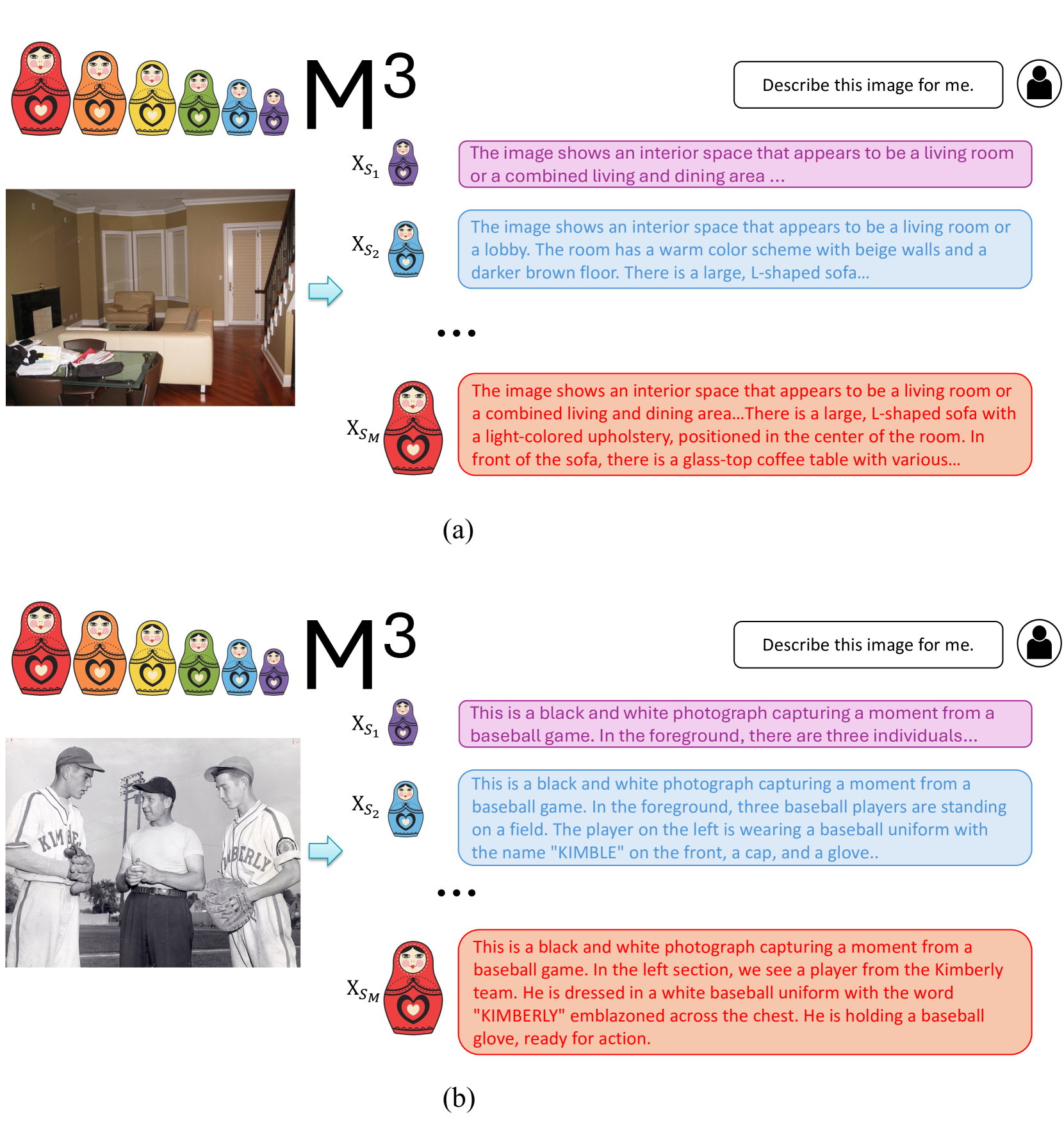<details> <summary>x5.png Details</summary>  ### Visual Description \n ## Diagram: M³ Model Image Description Process ### Overview The image is a two-part diagram (labeled (a) and (b)) illustrating the process of a model named "M³" generating textual descriptions for input images. Each part shows a different input image and a series of corresponding textual outputs, visualized using a metaphor of nested Matryoshka dolls. ### Components/Axes **General Layout (Both Parts):** * **Top Left:** A row of six colorful Matryoshka dolls, decreasing in size from left to right. Colors from left to right: red, orange, yellow, green, blue, purple. * **Top Center:** The label "**M³**" in large, bold, black font. * **Top Right:** A user icon (silhouette) next to a text box containing the prompt: "Describe this image for me." * **Left Column:** The input image. * **Center Column:** A vertical sequence of smaller Matryoshka dolls, each labeled with a mathematical notation (`X_S1`, `X_S2`, `...`, `X_SM`). These correspond to the dolls in the top row by color and order. * **Right Column:** A vertical sequence of colored text boxes, each aligned with a doll in the center column. The text boxes contain the generated descriptions. * **Flow Indicator:** A light blue arrow points from the input image to the sequence of dolls and descriptions. **Part (a) Specifics:** * **Input Image:** A color photograph of a living room interior. Visible elements include a beige L-shaped sofa, a glass-top coffee table, a fireplace, a staircase, and hardwood floors. * **Output Labels & Colors:** * `X_S1`: Purple doll, pink text box. * `X_S2`: Blue doll, light blue text box. * `X_SM`: Red doll, salmon/orange text box. * **Ellipsis:** Three black dots (`...`) are placed between the second and final output, indicating additional intermediate steps or outputs. **Part (b) Specifics:** * **Input Image:** A black and white photograph of three baseball players on a field. The player on the left has "KIMBLE" on his jersey. The player on the right has "KIMBERLY" on his jersey. * **Output Labels & Colors:** * `X_S1`: Purple doll, pink text box. * `X_S2`: Blue doll, light blue text box. * `X_SM`: Red doll, salmon/orange text box. * **Ellipsis:** Three black dots (`...`) are placed between the second and final output. ### Detailed Analysis / Content Details **Transcription of All Text:** **Part (a) Outputs:** 1. **`X_S1` (Pink Box):** "The image shows an interior space that appears to be a living room or a combined living and dining area ..." 2. **`X_S2` (Light Blue Box):** "The image shows an interior space that appears to be a living room or a lobby. The room has a warm color scheme with beige walls and a darker brown floor. There is a large, L-shaped sofa..." 3. **`X_SM` (Salmon Box):** "The image shows an interior space that appears to be a living room or a combined living and dining area...There is a large, L-shaped sofa with a light-colored upholstery, positioned in the center of the room. In front of the sofa, there is a glass-top coffee table with various..." **Part (b) Outputs:** 1. **`X_S1` (Pink Box):** "This is a black and white photograph capturing a moment from a baseball game. In the foreground, there are three individuals..." 2. **`X_S2` (Light Blue Box):** "This is a black and white photograph capturing a moment from a baseball game. In the foreground, three baseball players are standing on a field. The player on the left is wearing a baseball uniform with the name "KIMBLE" on the front, a cap, and a glove.." 3. **`X_SM` (Salmon Box):** "This is a black and white photograph capturing a moment from a baseball game. In the left section, we see a player from the Kimberly team. He is dressed in a white baseball uniform with the word "KIMBERLY" emblazoned across the chest. He is holding a baseball glove, ready for action." **Visual Progression:** * In both (a) and (b), the descriptions progress from a general, high-level summary (`X_S1`) to a more detailed and specific description (`X_S2`), culminating in the most detailed description (`X_SM`). * The final description (`X_SM`) in both cases includes specific object attributes (sofa color, table type) and precise text read from the image ("KIMBERLY"). ### Key Observations 1. **Metaphor of Nested Dolls:** The Matryoshka doll motif is used consistently to represent the model's outputs, suggesting a process of unpacking or revealing progressively more detailed information. 2. **Consistent Output Structure:** The model produces multiple descriptions (`S1` to `SM`) for a single image input, with each description offering a different level of detail. 3. **Increasing Specificity:** There is a clear trend from vague, categorical descriptions ("living room") to concrete, attribute-based descriptions ("beige walls," "glass-top coffee table," "word 'KIMBERLY' emblazoned"). 4. **Text Recognition Capability:** The model demonstrates the ability to perform optical character recognition (OCR) within its descriptions, as seen in part (b) with the jersey text. 5. **Color-Coding:** The outputs are color-coded to match the sequence of dolls, providing a visual link between the abstract model component (`X_S`) and its textual output. ### Interpretation This diagram illustrates the functionality of the "M³" model as a **multi-faceted image captioning or description system**. It does not produce a single description but rather a **spectrum of descriptions** varying in granularity. * **What it demonstrates:** The model appears to have an internal mechanism for generating descriptions at different levels of abstraction or from different "viewpoints," symbolized by the nested dolls. The progression from `X_S1` to `X_SM` suggests a pipeline or ensemble where initial, broad classifications are refined into detailed, grounded observations. * **Relationship between elements:** The input image is processed by the M³ model (represented by the doll sequence), which outputs a corresponding sequence of text descriptions. The user's prompt initiates this process. The ellipsis (`...`) implies the sequence is continuous or contains more steps than are explicitly shown. * **Notable implications:** This approach could be valuable for applications requiring adjustable detail levels (e.g., generating alt-text for the web, where a short and a long description are needed). It also highlights the model's capability for **visual grounding**—linking specific textual phrases ("glass-top coffee table") to visual elements in the image. The difference between the `X_S2` and `X_SM` descriptions in part (b) is particularly interesting; `X_S2` correctly reads "KIMBLE," while `X_SM` reads "KIMBERLY," which may indicate either an error or a different interpretation of the visual data, showcasing potential variability in the model's outputs. </details> Figure 6: More visualization examples. With more visual tokens, LMMs can discover more details, and generate higher quality descriptions. The images are from MSCOCO [17] validation set.