# Jina CLIP: Your CLIP Model Is Also Your Text Retriever
**Authors**: Andreas Koukounas, Georgios Mastrapas, Michael Günther, Bo Wang, Scott Martens, Isabelle Mohr, Saba Sturua, Mohammad Kalim Akram, Joan Fontanals Martínez, Saahil Ognawala, Susana Guzman, Maximilian Werk, Nan Wang, Han Xiao
Abstract
Contrastive Language-Image Pretraining (CLIP) is widely used to train models to align images and texts in a common embedding space by mapping them to fixed-sized vectors. These models are key to multimodal information retrieval and related tasks. However, CLIP models generally underperform in text-only tasks compared to specialized text models. This creates inefficiencies for information retrieval systems that keep separate embeddings and models for text-only and multimodal tasks. We propose a novel, multi-task contrastive training method to address this issue, which we use to train the jina-clip-v1 model and achieve the state-of-the-art performance on both text-image and text-text retrieval tasks.
Machine Learning, ICML, CLIP, Embeddings, Multimodal, Retrieval
1 Introduction
Text-image contrastively trained models, such as CLIP (Radford et al., 2021), create an aligned representation space for images and texts by leveraging pairs of images and their corresponding captions. Similarly, text-text contrastively trained models, like jina-embeddings-v2 (Günther et al., 2023), construct a representation space for semantically similar texts using pairs of related texts such as question/answer pairs, query/document pairs, or other text pairs with known semantic relationships.
Because image captions are typically very short, CLIP-style models trained with them only support short text context lengths. They struggle to capture the richer information in longer texts, and as a result, perform poorly on text-only tasks. Our empirical study (Table 1) demonstrates that OpenAI’s CLIP underperforms in all text retrieval tasks. This poses problems for many applications that use larger text inputs, like text-image retrieval, multimodal retrieval augmented generation (Zhao et al., 2023) and image generation.
In this paper, we present and demonstrate the effectiveness of a novel approach to contrastive training with large-scale image-caption pairs and text pairs. We jointly optimize for representation alignment of both text-image and text-text pairs, enabling the model to perform well at both kinds of tasks. Due to the lack of available multimodal multi-target datasets (e.g. text-text-image triplets) we use different datasets for each class of task and jointly train for both.
The resulting model, jina-clip-v1, performs comparably to EVA-CLIP (Sun et al., 2023) on the cross-modal CLIP Benchmark https://github.com/LAION-AI/CLIP_benchmark, while the text encoder by itself performs as well as similar models on MTEB Benchmark tasks (Muennighoff et al., 2023).
<details>
<summary>x1.png Details</summary>
### Visual Description
## Diagram: Multi-Task Learning for Text-Image Similarity
### Overview
The image presents a diagram illustrating a multi-task learning approach for jointly optimizing text-text and text-image similarity. It shows three distinct tasks, each with its own data inputs, encoders, loss functions, and optimization steps. The tasks are numbered 1, 2, and 3, and each involves a combination of text and image data.
### Components/Axes
* **Legend (Top-Left)**:
* Orange Arrow: Task 1: Align Text-Text Embeddings
* Blue Arrow: Task 2: Align Text-Image Embeddings
* **Task 1 (Left)**: Jointly optimize text-text and short caption-image similarity
* **Task 2 (Center)**: Jointly optimize text-text and long caption-image similarity
* **Task 3 (Right)**: Jointly optimize text-triplets (anchor, pos, neg) and long caption-image similarity
### Detailed Analysis
**Task 1: Jointly optimize text-text and short caption-image similarity**
* **Input 1**: "Text Pairs" (represented by two stacked documents) connected by an orange arrow to "Text Encoder" (blue rectangle).
* **Input 2**: "Short Captions" (represented by one document) connected by a blue arrow to "Text Encoder" (blue rectangle).
* **Input 3**: Image (represented by an image icon) connected by a blue arrow to "Image Encoder" (green rectangle).
* **Process 1**: Output of "Text Encoder" (from "Text Pairs") connected by an orange arrow to "InfoNCE+" (white rectangle).
* **Process 2**: Output of "InfoNCE+" connected by an orange arrow to "Sum & Backward" (white rectangle).
* **Process 3**: Output of "Text Encoder" (from "Short Captions") connected by a blue arrow to "CLIP Loss" (white rectangle).
* **Process 4**: Output of "Image Encoder" connected by a blue arrow to "CLIP Loss" (white rectangle).
* **Process 5**: Output of "CLIP Loss" connected by a blue arrow to "Sum & Backward" (white rectangle).
**Task 2: Jointly optimize text-text and long caption-image similarity**
* **Input 1**: "Text Pairs" (represented by two stacked documents) connected by an orange arrow to "Text Encoder" (blue rectangle).
* **Input 2**: "Long Captions" (represented by one document) connected by a blue arrow to "Text Encoder" (blue rectangle).
* **Input 3**: Image (represented by an image icon) connected by a blue arrow to "Image Encoder" (green rectangle).
* **Process 1**: Output of "Text Encoder" (from "Text Pairs") connected by an orange arrow to "InfoNCE+" (white rectangle).
* **Process 2**: Output of "InfoNCE+" connected by an orange arrow to "Sum & Backward" (white rectangle).
* **Process 3**: Output of "Text Encoder" (from "Long Captions") connected by a blue arrow to "CLIP Loss" (white rectangle).
* **Process 4**: Output of "Image Encoder" connected by a blue arrow to "CLIP Loss" (white rectangle).
* **Process 5**: Output of "CLIP Loss" connected by a blue arrow to "Sum & Backward" (white rectangle).
**Task 3: Jointly optimize text-triplets (anchor, pos, neg) and long caption-image similarity**
* **Input 1**: "Text Triplets" (represented by three stacked documents) connected by an orange arrow to "Text Encoder" (blue rectangle).
* **Input 2**: "Long Captions" (represented by one document) connected by a blue arrow to "Text Encoder" (blue rectangle).
* **Input 3**: Image (represented by an image icon) connected by a blue arrow to "Image Encoder" (green rectangle).
* **Process 1**: Output of "Text Encoder" (from "Text Triplets") connected by an orange arrow to "InfoNCE+" (white rectangle).
* **Process 2**: Output of "InfoNCE+" connected by an orange arrow to "Sum & Backward" (white rectangle).
* **Process 3**: Output of "Text Encoder" (from "Long Captions") connected by a blue arrow to "CLIP Loss" (white rectangle).
* **Process 4**: Output of "Image Encoder" connected by a blue arrow to "CLIP Loss" (white rectangle).
* **Process 5**: Output of "CLIP Loss" connected by a blue arrow to "Sum & Backward" (white rectangle).
### Key Observations
* All three tasks utilize a "Text Encoder" and an "Image Encoder."
* Tasks 1, 2, and 3 use "InfoNCE+" and "CLIP Loss" components.
* Tasks 1 uses "Text Pairs" and "Short Captions" as text inputs, while Tasks 2 and 3 use "Text Pairs" and "Long Captions" as text inputs. Task 3 also uses "Text Triplets".
* All tasks end with a "Sum & Backward" operation.
* The orange arrows represent the flow of text-text embeddings, while the blue arrows represent the flow of text-image embeddings.
### Interpretation
The diagram illustrates a multi-task learning framework designed to improve text-image similarity by jointly optimizing different objectives. Each task focuses on a specific combination of text and image data, allowing the model to learn more robust and generalizable representations. The use of "InfoNCE+" and "CLIP Loss" suggests that the model is trained to maximize the similarity between related text and images while minimizing the similarity between unrelated ones. The "Sum & Backward" operation likely represents the aggregation of losses from different components and the subsequent backpropagation of gradients for model training. The differences in text inputs ("Text Pairs," "Short Captions," "Long Captions," and "Text Triplets") indicate that the model is designed to handle various types of text data, including paired text, short captions, long captions, and triplets of text (anchor, positive, negative).
</details>
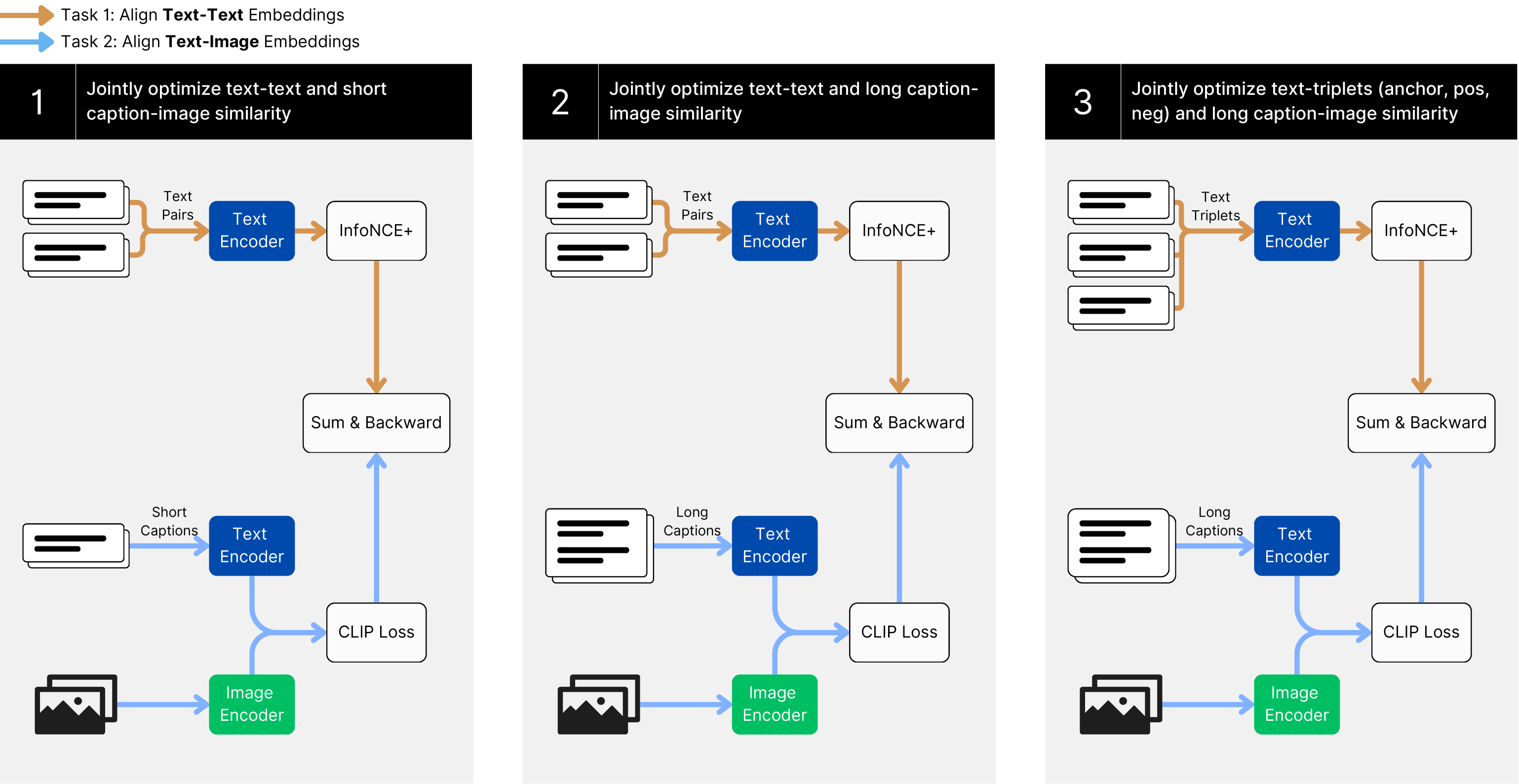
Figure 1: The training paradigm of jina-clip-v1 , jointly optimizing text-image and text-text matching.
2 Related Work
Contrastive learning for text embeddings is well-established for training models for text-based information retrieval, semantic textual similarity, text clustering, and re-ranking. Reimers & Gurevych (2019) propose a dual encoder architecture for pairwise text similarity training. Ni et al. (2022) demonstrate that the dual-encoder architecture scales efficiently. Wang et al. (2022) and Günther et al. (2023) develop multi-stage training methods incorporating hard negatives. Mohr et al. (2024) bring textual similarity scores directly into the training. Günther et al. (2023) and Chen et al. (2024) extend text embedding models’ maximum input length to 8,192 tokens.
Contrastive text-image pre-training has become increasingly popular since Radford et al. (2021) proposed the CLIP (Contrastive Language-Image Pre-training) paradigm. Numerous follow-up studies have sought to improve text-image training. Zhai et al. (2022) introduce locked image tuning (LiT), which involves fixing the weights of a trained image encoder and training a text encoder to align with its image representations. Kossen et al. (2023) generalize the LiT paradigm to a more flexible Three Tower architecture. Zhai et al. (2023) propose a modified sigmoid loss function for contrastive learning, demonstrating better performance on relatively small batch sizes. Cherti et al. (2023) and Sun et al. (2023) explore different setups for text-image training, including variations in datasets, model size, and hyperparameters. Zhang et al. (2024) empirically determine that the effective context length of CLIP is less than 20 tokens and propose an algorithm to stretch the positional encoding, improving performance on longer texts. Sun et al. (2024) scale up the EVA-CLIP architecture to 18B parameters.
Furthermore, a growing number of large datasets, such as YFCC100M (Thomee et al., 2016), LAION-5B (Schuhmann et al., 2022), and curated datasets like ShareGPT4v (Chen et al., 2023) help to constantly improve the performance of CLIP-like models.
3 Model Architecture
We use the same dual encoder architecture introduced in the original CLIP (Radford et al., 2021). It comprises a text encoder and an image encoder that generate representations of identical dimensionality.
The text encoder uses the JinaBERT architecture (Günther et al., 2023), a BERT variant that integrates AliBi (Press et al., 2021) to support longer texts. We pre-train the model using the Masked Language Modeling objective from the original BERT model (Devlin et al., 2019). Experimental results indicate that this yields superior final performance compared to starting from a text embedding model that has already been fully trained using contrastive learning.
For the image encoder, we use the EVA02 architecture (Fang et al., 2023). To keep the model size comparable to the text encoder, we select the base variant and initialize our model with the EVA02 pre-trained weights. Our experiments show that EVA02 significantly outperforms comparable image encoders like DinoV2 (Oquab et al., 2024) and ViT B/16 models from OpenCLIP (Ilharco et al., 2021).
4 Training
Figure 1 illustrates our multi-task, three-stage training approach. This method jointly optimizes the model to perform two tasks: text-image matching and text-text matching.
To achieve text retrieval performance on par with state-of-the-art text embedding models, we employ a multi-stage training paradigm, similar to what Wang et al. (2022) and Günther et al. (2023) propose. This paradigm introduces a second training stage, analogous to conventional fine-tuning stages, that makes use of small high-quality datasets with hard negatives to improve performance on embedding tasks.
We complement the two stages with text-image pairs for a two-task two-stage training pipeline. To address the short effective context length of CLIP-like models, we introduce an intermediate stage for training on long captions. Due to limited availability of public data, we rely on AI-generated long textual descriptions for this stage. The reasoning behind opting for a separate stage is two-fold: a) because of the dataset size difference, integrating this data into the pre-training stage will limit its impact, and b) using the triplet fine-tuning stage for long caption training will limit the effect of hard negatives, as the model is not yet able to effectively process long contexts.
The result is a three-stage training process with two tasks in each stage:
- Stage 1 focuses on learning to align image and text representations while minimizing losses in text-text performance. To this end, we train on large-scale and weakly supervised text-image and text-text pair datasets.
- Stage 2 presents longer, synthetic image captions to the model while continuing to train with text-text pairs.
- Stage 3 uses hard negatives to further improve the text encoder in separating relevant from irrelevant text. To maintain text-image alignment, we continue training on long image captions.
4.1 Data Preparation
Our text pair corpus $\mathbb{C}^{\mathit{text}}_{\mathit{pairs}}$ consists of data from a diverse collection of 40 text-pair datasets, similar to the corpus used in Günther et al. (2023).
For text-image training in Stage 1, we use LAION-400M (Schuhmann et al., 2021) as our corpus $\mathbb{C}^{\mathit{img(s)}}_{\mathit{pairs}}$ . LAION-400M contains 400M image-text pairs derived from Common Crawl and is widely used for multimodal training.
In Stages 2 and 3, we use the ShareGPT4V (Chen et al., 2023) dataset as our $\mathbb{C}^{\mathit{img(l)}}_{\mathit{pairs}}$ corpus. This dataset contains approximately 100K synthetic captions generated with GPT4v (OpenAI, 2023) and an additional 1.1M long captions generated by a large captioning model trained on the original GPT4v generated output. This comes to a total of roughly 1.2M image captions. It would be interesting to investigate the impact of AI-generated data on performance, but that is outside the scope of this work.
Finally, in Stage 3, we use a triplet text corpus $\mathbb{C}^{\mathit{text}}_{\mathit{triplets}}$ that includes hard negatives. This corpus combines data from MSMarco (Bajaj et al., 2016), Natural Questions (NQ) (Kwiatkowski et al., 2019), HotpotQA (Yang et al., 2018) and the Natural Language Inference (NLI) dataset (Bowman et al., 2015). Each training batch contains one annotated positive and seven negative items. We select hard negatives using text retrieval models to emphasize relevance in text triplets, except for NLI where negatives are chosen randomly.
4.2 Loss Functions
All three stages employ a joint loss function that combines two InfoNCE loss functions (Van den Oord et al., 2018). For the text pairs in stage 1 and stage 2, we use the $\mathcal{L}_{\mathrm{nce}}$ loss function of pairs of text embeddings $(\bf{q},\bf{p})\sim\mathbf{B}$ within a batch $\mathbf{B}⊂\mathbb{D}^{\mathrm{pairs}}$ . This function evaluates the cosine similarity $cos(\bf{q},\bf{p})$ between a given query $q$ and its corresponding target $p$ , relative to the similarity of all other targets in the batch. We sum the loss in both directions to preserve the symmetry of similarity measures:
$$
\displaystyle\mathcal{L}_{\mathrm{nce}}(\mathbf{B}):=\mathcal{L}_{\mathrm{nce}%
}^{\longrightarrow}(\mathbf{B})+\mathcal{L}_{\mathrm{nce}}^{\longleftarrow}(%
\mathbf{B}),\text{ with} \displaystyle\mathcal{L}_{\mathrm{nce}}^{\longrightarrow}(\mathbf{B}):=\mathbb%
{E}_{(\bf{q},\bf{p})\sim\mathbf{B}}\left[-\ln\frac{e^{cos(\bf{q},\bf{p})/\tau}%
}{\sum\limits_{i=1}^{k}e^{cos(\bf{q},\bf{p_{i}})/\tau}}\right] \displaystyle\mathcal{L}_{\mathrm{nce}}^{\longleftarrow}(\mathbf{B}):=\mathbb{%
E}_{(\bf{q},p)\sim\mathbf{B}}\left[-\ln\frac{e^{cos(\bf{p},\bf{q})/\tau}}{\sum%
\limits_{i=1}^{k}e^{cos(\bf{p},\bf{q_{i}})/\tau}}\right] \tag{1}
$$
The constant temperature parameter $\tau$ influences how the loss function weighs minor differences in the similarity scores (Wang & Liu, 2021). In accordance with related work (Günther et al., 2023), we choose $\tau=0.05$ .
Similarly, we apply $\mathcal{L}_{\mathrm{nce}}$ to pairs of caption and image embeddings $(\bf{c},\bf{i})\sim\mathbf{B}$ in batches $\mathbf{B}⊂\mathbb{D}^{\mathrm{img}}$ to obtain loss values for text-image matching. For text-image training, $\tau$ is trainable, following the default behaviour in the OpenCLIP framework (Ilharco et al., 2021).
For text-text training in stage 3, we use text embeddings from the triplet database $(\bf{q},\bf{p},\bf{n_{1}}...,\bf{n_{7}})\sim\mathbf{B}$ drawn in batches $\mathbf{B}⊂\mathbb{D}^{\mathrm{triplets}}$ . Recall that these consist of a query $\bf{q}$ , a positive match $\bf{p}$ , and seven negatives $\bf{n_{1}}...,\bf{n_{7}}$ . We employ an extended version of the $\mathcal{L}_{\mathrm{nce}}$ loss, denoted here as $\mathcal{L}_{\mathrm{nce}^{+}}$ , in Equation (2). Similar to $\mathcal{L}_{\mathrm{nce}}$ , this loss function is bidirectional but incorporates additional negatives when pairing queries with passages:
$$
\displaystyle\mathcal{L}_{\mathrm{nce}^{+}}(\mathbf{B}):= \displaystyle\;\;\;\;\;\mathbb{E}_{r\sim\mathbf{B}}\Bigg{[}-\ln\frac{e^{cos(%
\bf{q},\bf{p})/\tau}}{\sum\limits_{i=1}^{k}\Big{[}e^{cos(\bf{q},p_{i})/\tau}+%
\sum\limits_{j=1}^{7}e^{cos(\bf{q},\bf{n_{j,i}})/\tau}\Big{]}}\Bigg{]} \displaystyle\,+\mathbb{E}_{r\sim\mathbf{B}}\Bigg{[}-\ln\frac{e^{cos(\bf{p},%
\bf{q})/\tau}}{\sum\limits_{i=1}^{k}e^{cos(\bf{p},\bf{q_{i}})/\tau}}\Bigg{]} \displaystyle\text{with}\;r=(\bf{q},\bf{p},\bf{n_{1}},\ldots,\bf{n_{7}}). \tag{2}
$$
4.3 Training Steps
In each stage, the text and image encoders are applied to inputs from the corpora described in Section 4.1 and the training uses the following combinations of loss functions:
$$
\displaystyle\mathcal{L}_{1}(\mathbf{B_{\mathit{text;s}}},\mathbf{B_{\mathit{%
img;s}}}):=\mathcal{L}_{\mathrm{nce}}(\mathbf{B_{\mathit{text;s}}})+\mathcal{L%
}_{\mathrm{nce}}(\mathbf{B_{\mathit{img;s}}}) \displaystyle\mathcal{L}_{2}(\mathbf{B_{\mathit{text;l}}},\mathbf{B_{\mathit{%
img;l}}}):=\mathcal{L}_{\mathrm{nce}}(\mathbf{B_{\mathit{text;l}}})+\mathcal{L%
}_{\mathrm{nce}}(\mathbf{B_{\mathit{img;l}}}) \displaystyle\mathcal{L}_{3}(\mathbf{B_{\mathit{text3}}},\mathbf{B_{\mathit{%
img;l}}}):=\mathcal{L}_{\mathrm{nce}}(\mathbf{B_{\mathit{text3}}})+\mathcal{L}%
_{\mathrm{nce}^{+}}(\mathbf{B_{\mathit{img;l}}}) \tag{3}
$$
For stage 1, $\mathbf{B_{\mathit{text;s}}}$ is obtained from $\mathbb{C}^{\mathit{text}}_{\mathit{pairs}}$ by truncating the text values during tokenization to $77$ tokens as in Radford et al. (2021). This enables us to use very large batches of size $32,768$ . $\mathbf{B_{\mathit{img;s}}}$ is obtained from $\mathbb{C}^{\mathit{img(s)}}_{\mathit{pairs}}$ with the same truncation, albeit most captions in this corpus are short.
For stage 2, $\mathbb{C}^{\mathit{text}}_{\mathit{pairs}}$ is used again. However, text values are truncated to 512 tokens in this case, and as a result a smaller batch size of $8,192$ is used. The text image pairs $\mathbf{B_{\mathit{img;l}}}$ are selected from $\mathbb{C}^{\mathit{img(l)}}_{\mathit{pairs}}$ . During this stage, text-text and text-image retrieval improves by adding synthetic data with longer captions to the training.
The last stage uses text triplets from $\mathbb{C}^{\mathit{text}}_{\mathit{triplets}}$ and the text-image batches $\mathbf{B_{\mathit{img;l}}}$ as in stage 2. This focused fine-tuning using text triplets and hard negatives brings text-text performance up to competitive levels with specialized text-only models. Training settings as well as training times for each stage are given in detail in Appendix table 2.
5 Evaluation
Table 1: Evaluation results on CLIP Benchmark and MTEB
| Benchmark Task Type Model - Metric | CLIP Benchmark Zero-Shot Retrieval txt-img r@5 | MTEB Retrieval img-txt r@5 | STS-r@5 | Avg MTEB Score-ndcg@10 | spearman | score |
| --- | --- | --- | --- | --- | --- | --- |
| OpenAI CLIP ViT B/16 | 75.62 | 88.12 | 15.88 | 17.63 | 66.22 | 43.95 |
| EVA-CLIP ViT B/16 | 82.15 | 90.59 | 22.92 | 26.03 | 69.62 | 47.64 |
| LongCLIP ViT B/16 | 81.72 | 90.79 | 25.96 | 28.76 | 68.57 | 47.71 |
| jina-embeddings-v2 | - | - | 42.56 | 47.85 | 80.70 | 60.38 |
| jina-clip-v1 stage 1 | 78.05 | 86.95 | 36.29 | 39.52 | 77.96 | 56.51 |
| jina-clip-v1 stage 2 | 81.86 | 90.59 | 36.80 | 40.44 | 78.33 | 57.19 |
| jina-clip-v1 | 80.31 | 89.91 | 43.05 | 48.33 | 80.92 | 60.12 |
txt-img r@5 : Text to Image Recall@5 [%] img-txt r@5 : Image to Text Recall@5 [%] r@5 : Recall@5 [%] spearman: Spearman Correlation
We evaluate our model’s performance on text-only tasks, image-only tasks, and cross-modal tasks with both text and images. Table 1 shows the results of tests comparing jina-clip-v1 to OpenAI CLIP (Radford et al., 2021), EVA-CLIP (Sun et al., 2023), and LongCLIP ViT B/16 (Zhang et al., 2024) models. Additionally, for text retrieval performance, we include a comparison with jina-embeddings-v2. These results demonstrate our model’s high performance across all benchmarks.
To evaluate the model’s cross-modal performance, we use the CLIP Benchmark which includes zero-shot image-classification and zero-shot cross-modal retrieval tasks. For zero-shot image-text and text-image information retrieval, we evaluate using Flickr8k (Hodosh et al., 2013), Flickr30K (Young et al., 2014) and MSCOCO Captions (Chen et al., 2015), which are all included in CLIP Benchmark. jina-clip-v1 achieves an average Recall@5 of 85.8% across all retrieval benchmarks, outperforming OpenAI’s CLIP model and performing on par with EVA-CLIP.
To evaluate jina-clip-v1 ’s text encoder, we use the Massive Text Embedding Benchmark (MTEB) (Muennighoff et al., 2023), which includes eight tasks involving 58 datasets. CLIP-like models generally perform poorly on text embedding tasks, particularly information retrieval. However, jina-clip-v1 competes closely with top-tier text-only embedding models, achieving an average score of 60.12%. This improves on other CLIP models by roughly 15% overall and 22% in retrieval tasks. Detailed results are provided in the appendix.
6 Conclusion
We have presented a multi-task, three-stage training method that enables multimodal models to retain high levels of performance on text-only tasks. The model we produced using this method, jina-clip-v1, exhibits strong performance in cross-modal tasks like text-image retrieval and excels in tasks like semantic textual similarity and text retrieval. This result confirms that unified multimodal models can replace separate models for different task modalities, with large potential savings for applications. This model is currently limited to English-language texts due to limited multilingual resources. Future work will focus on extending this work to multilingual contexts.
References
- Bajaj et al. (2016) Bajaj, P., Campos, D., Craswell, N., Deng, L., Gao, J., Liu, X., Majumder, R., McNamara, A., Mitra, B., Nguyen, T., et al. MS MARCO: A Human Generated MAchine Reading COmprehension Dataset. arXiv preprint arXiv:1611.09268, 2016. URL https://arxiv.org/abs/1611.09268.
- Bowman et al. (2015) Bowman, S., Angeli, G., Potts, C., and Manning, C. D. A large annotated corpus for learning natural language inference. In Proceedings of the 2015 Conference on Empirical Methods in Natural Language Processing, pp. 632–642, 2015. doi: 10.18653/v1/D15-1075. URL https://aclanthology.org/D15-1075.
- Chen et al. (2024) Chen, J., Xiao, S., Zhang, P., Luo, K., Lian, D., and Liu, Z. BGE M3-Embedding: Multi-Lingual, Multi-Functionality, Multi-Granularity Text Embeddings Through Self-Knowledge Distillation. arXiv preprint arXiv:2402.03216, 2024. URL https://arxiv.org/abs/2402.03216.
- Chen et al. (2023) Chen, L., Li, J., Dong, X., Zhang, P., He, C., Wang, J., Zhao, F., and Lin, D. ShareGPT4V: Improving Large Multi-Modal Models with Better Captions. arXiv preprint arXiv:2311.12793, 2023. URL https://arxiv.org/abs/2311.12793.
- Chen et al. (2015) Chen, X., Fang, H., Lin, T., Vedantam, R., Gupta, S., Dollár, P., and Zitnick, C. L. Microsoft COCO Captions: Data Collection and Evaluation Server. arXiv preprint arXiv:1504.00325, 2015. URL http://arxiv.org/abs/1504.00325.
- Cherti et al. (2023) Cherti, M., Beaumont, R., Wightman, R., Wortsman, M., Ilharco, G., Gordon, C., Schuhmann, C., Schmidt, L., and Jitsev, J. Reproducible Scaling Laws for Contrastive Language-Image Learning. In 2023 IEEE/CVF Conference on Computer Vision and Pattern Recognition (CVPR), pp. 2818–2829, 2023. doi: 10.1109/CVPR52729.2023.00276. URL https://doi.ieeecomputersociety.org/10.1109/CVPR52729.2023.00276.
- Devlin et al. (2019) Devlin, J., Chang, M., Lee, K., and Toutanova, K. BERT: Pre-training of Deep Bidirectional Transformers for Language Understanding. In Burstein, J., Doran, C., and Solorio, T. (eds.), Proceedings of the 2019 Conference of the North American Chapter of the Association for Computational Linguistics: Human Language Technologies, NAACL-HLT 2019, pp. 4171–4186. Association for Computational Linguistics, 2019. doi: 10.18653/V1/N19-1423. URL https://doi.org/10.18653/v1/n19-1423.
- Fang et al. (2023) Fang, Y., Sun, Q., Wang, X., Huang, T., Wang, X., and Cao, Y. EVA-02: A Visual Representation for Neon Genesis. arXiv preprint arXiv:2303.11331, 2023. URL https://arxiv.org/abs/2303.11331.
- Günther et al. (2023) Günther, M., Mastrapas, G., Wang, B., Xiao, H., and Geuter, J. Jina Embeddings: A Novel Set of High-Performance Sentence Embedding Models. In Tan, L., Milajevs, D., Chauhan, G., Gwinnup, J., and Rippeth, E. (eds.), Proceedings of the 3rd Workshop for Natural Language Processing Open Source Software (NLP-OSS 2023), pp. 8–18, Singapore, 2023. Association for Computational Linguistics. doi: 10.18653/v1/2023.nlposs-1.2. URL https://aclanthology.org/2023.nlposs-1.2.
- Günther et al. (2023) Günther, M., Ong, J., Mohr, I., Abdessalem, A., Abel, T., Akram, M. K., Guzman, S., Mastrapas, G., Sturua, S., Wang, B., Werk, M., Wang, N., and Xiao, H. Jina Embeddings 2: 8192-Token General-Purpose Text Embeddings for Long Documents. arXiv preprint arXiv:2310.19923, 2023. URL https://arxiv.org/abs/2310.19923.
- Hodosh et al. (2013) Hodosh, M., Young, P., and Hockenmaier, J. Framing Image Description as a Ranking Task: Data, Models and Evaluation Metrics. Journal of Artificial Intelligence Research, 47:853–899, 2013. doi: 10.1613/jair.3994. URL https://www.jair.org/index.php/jair/article/view/10833.
- Ilharco et al. (2021) Ilharco, G., Wortsman, M., Wightman, R., Gordon, C., Carlini, N., Taori, R., Dave, A., Shankar, V., Namkoong, H., Miller, J., Hajishirzi, H., Farhadi, A., and Schmidt, L. OpenCLIP (0.1). Zenodo, 2021. doi: 10.5281/zenodo.5143773. URL https://doi.org/10.5281/zenodo.5143773. Software.
- Kossen et al. (2023) Kossen, J., Collier, M., Mustafa, B., Wang, X., Zhai, X., Beyer, L., Steiner, A., Berent, J., Jenatton, R., and Kokiopoulou, E. Three Towers: Flexible Contrastive Learning with Pretrained Image Models. arXiv preprint arXiv:2305.16999, 2023. URL https://arxiv.org/abs/2305.16999.
- Kwiatkowski et al. (2019) Kwiatkowski, T., Palomaki, J., Redfield, O., Collins, M., Parikh, A., Alberti, C., Epstein, D., Polosukhin, I., Kelcey, M., Devlin, J., Lee, K., Toutanova, K. N., Jones, L., Chang, M.-W., Dai, A., Uszkoreit, J., Le, Q., and Petrov, S. Natural Questions: a Benchmark for Question Answering Research. Transactions of the Association of Computational Linguistics, 7:452–466, 2019. doi: 10.1162/tacl˙a˙00276. URL https://aclanthology.org/Q19-1026.
- Loshchilov & Hutter (2017) Loshchilov, I. and Hutter, F. Fixing Weight Decay Regularization in Adam. arXiv preprint arXiv:1711.05101v1, 2017. URL https://arxiv.org/abs/1711.05101v1.
- Mohr et al. (2024) Mohr, I., Krimmel, M., Sturua, S., Akram, M. K., Koukounas, A., Günther, M., Mastrapas, G., Ravishankar, V., Martínez, J. F., Wang, F., Liu, Q., Yu, Z., Fu, J., Ognawala, S., Guzman, S., Wang, B., Werk, M., Wang, N., and Xiao, H. Multi-Task Contrastive Learning for 8192-Token Bilingual Text Embeddings. arXiv preprint arXiv:2310.19923, 2024. URL https://arxiv.org/abs/2402.17016.
- Muennighoff et al. (2023) Muennighoff, N., Tazi, N., Magne, L., and Reimers, N. MTEB: Massive Text Embedding Benchmark. pp. 2014–2037, 2023. doi: 10.18653/v1/2023.eacl-main.148. URL https://aclanthology.org/2023.eacl-main.148.
- Ni et al. (2022) Ni, J., Qu, C., Lu, J., Dai, Z., Ábrego, G. H., Ma, J., Zhao, V. Y., Luan, Y., Hall, K. B., Chang, M., and Yang, Y. Large Dual Encoders Are Generalizable Retrievers. In Proceedings of the 2022 Conference on Empirical Methods in Natural Language Processing, EMNLP 2022, pp. 9844–9855, 2022. doi: 10.18653/V1/2022.EMNLP-MAIN.669. URL https://doi.org/10.18653/v1/2022.emnlp-main.669.
- OpenAI (2023) OpenAI. GPT-4 Technical Report. arXiv preprint arXiv:2303.08774, 2023. URL https://arxiv.org/abs/2303.08774.
- Oquab et al. (2024) Oquab, M., Darcet, T., Moutakanni, T., Vo, H., Szafraniec, M., Khalidov, V., Fernandez, P., Haziza, D., Massa, F., El-Nouby, A., Assran, M., Ballas, N., Galuba, W., Howes, R., Huang, P.-Y., Li, S.-W., Misra, I., Rabbat, M., Sharma, V., Synnaeve, G., Xu, H., Jegou, H., Mairal, J., Labatut, P., Joulin, A., and Bojanowski, P. DINOv2: Learning Robust Visual Features without Supervision. arXiv preprint arXiv:2304.07193, 2024. URL https://arxiv.org/abs/2304.07193.
- Press et al. (2021) Press, O., Smith, N. A., and Lewis, M. Train Short, Test Long: Attention with Linear Biases Enables Input Length Extrapolation. arXiv preprint arXiv:2108.12409, 2021. URL https://arxiv.org/abs/2108.12409.
- Radford et al. (2021) Radford, A., Kim, J. W., Hallacy, C., Ramesh, A., Goh, G., Agarwal, S., Sastry, G., Askell, A., Mishkin, P., Clark, J., Krueger, G., and Sutskever, I. Learning Transferable Visual Models From Natural Language Supervision. pp. 8748–8763, 2021. URL https://proceedings.mlr.press/v139/radford21a.html.
- Reimers & Gurevych (2019) Reimers, N. and Gurevych, I. Sentence-BERT: Sentence Embeddings using Siamese BERT-Networks. In Inui, K., Jiang, J., Ng, V., and Wan, X. (eds.), Proceedings of the 2019 Conference on Empirical Methods in Natural Language Processing, pp. 3980–3990. Association for Computational Linguistics, 2019. doi: 10.18653/V1/D19-1410. URL https://doi.org/10.18653/v1/D19-1410.
- Schuhmann et al. (2021) Schuhmann, C., Vencu, R., Beaumont, R., Kaczmarczyk, R., Mullis, C., Katta, A., Coombes, T., Jitsev, J., and Komatsuzaki, A. LAION-400M: Open Dataset of CLIP-Filtered 400 Million Image-Text Pairs. arXiv preprint arXiv:2111.02114, 2021. URL https://arxiv.org/abs/2111.02114.
- Schuhmann et al. (2022) Schuhmann, C., Beaumont, R., Vencu, R., Gordon, C. W., Wightman, R., Cherti, M., Coombes, T., Katta, A., Mullis, C., Wortsman, M., Schramowski, P., Kundurthy, S. R., Crowson, K., Schmidt, L., Kaczmarczyk, R., and Jitsev, J. LAION-5B: An open large-scale dataset for training next generation image-text models. In Koyejo, S., Mohamed, S., Agarwal, A., Belgrave, D., Cho, K., and Oh, A. (eds.), Advances in Neural Information Processing Systems 35 (NeurIPS 2022) Datasets and Benchmarks Track, volume 35, pp. 25278–25294, 2022.
- Sun et al. (2023) Sun, Q., Fang, Y., Wu, L., Wang, X., and Cao, Y. EVA-CLIP: Improved Training Techniques for CLIP at Scale. arXiv preprint arXiv:2303.15389, 2023. URL https://arxiv.org/abs/2303.15389.
- Sun et al. (2024) Sun, Q., Wang, J., Yu, Q., Cui, Y., Zhang, F., Zhang, X., and Wang, X. EVA-CLIP-18B: Scaling CLIP to 18 Billion Parameters. arXiv preprint arXiv:2402.04252, 2024. URL https://arxiv.org/abs/2402.04252.
- Thomee et al. (2016) Thomee, B., Shamma, D. A., Friedland, G., Elizalde, B., Ni, K., Poland, D., Borth, D., and Li, L. YFCC100M: The New Data in Multimedia Research. Communications of the ACM, 59(2):64–73, 2016. doi: 10.1145/2812802. URL https://doi.org/10.1145/2812802.
- Van den Oord et al. (2018) Van den Oord, A., Li, Y., and Vinyals, O. Representation Learning with Contrastive Predictive Coding. arXiv preprint arXiv:1807.03748, 2018. URL http://arxiv.org/abs/1807.03748.
- Wang & Liu (2021) Wang, F. and Liu, H. Understanding the Behaviour of Contrastive Loss. In 2021 IEEE/CVF Conference on Computer Vision and Pattern Recognition (CVPR), pp. 2495–2504, 2021. doi: 10.1109/CVPR46437.2021.00252. URL https://ieeexplore.ieee.org/document/9577669.
- Wang et al. (2022) Wang, L., Yang, N., Huang, X., Jiao, B., Yang, L., Jiang, D., Majumder, R., and Wei, F. Text Embeddings by Weakly-Supervised Contrastive Pre-training. arXiv preprint arXiv:2212.03533, 2022. URL https://arxiv.org/abs/2212.03533.
- Yang et al. (2018) Yang, Z., Qi, P., Zhang, S., Bengio, Y., Cohen, W. W., Salakhutdinov, R., and Manning, C. D. HotpotQA: A Dataset for Diverse, Explainable Multi-hop Question Answering. In Riloff, E., Chiang, D., Hockenmaier, J., and Tsujii, J. (eds.), Proceedings of the 2018 Conference on Empirical Methods in Natural Language Processing, EMNLP 2018, pp. 2369–2380, 2018. doi: 10.18653/V1/D18-1259. URL https://doi.org/10.18653/v1/d18-1259.
- Young et al. (2014) Young, P., Lai, A., Hodosh, M., and Hockenmaier, J. From image descriptions to visual denotations: New similarity metrics for semantic inference over event descriptions. Transactions of the Association for Computational Linguistics, 2:67–78, 2014. doi: 10.1162/tacl˙a˙00166. URL https://aclanthology.org/Q14-1006.
- Zhai et al. (2022) Zhai, X., Wang, X., Mustafa, B., Steiner, A., Keysers, D., Kolesnikov, A., and Beyer, L. LiT: Zero-Shot Transfer with Locked-image text Tuning. In IEEE/CVF Conference on Computer Vision and Pattern Recognition, CVPR 2022, pp. 18102–18112. IEEE, 2022. doi: 10.1109/CVPR52688.2022.01759. URL https://doi.org/10.1109/CVPR52688.2022.01759.
- Zhai et al. (2023) Zhai, X., Mustafa, B., Kolesnikov, A., and Beyer, L. Sigmoid Loss for Language Image Pre-Training. arXiv preprint arXiv:2303.15343, 2023. URL https://arxiv.org/abs/2303.15343.
- Zhang et al. (2024) Zhang, B., Zhang, P., Dong, X., Zang, Y., and Wang, J. Long-CLIP: Unlocking the Long-Text Capability of CLIP. arXiv preprint arXiv:2403.15378, 2024. URL https://arxiv.org/abs/2403.15378.
- Zhao et al. (2023) Zhao, R., Chen, H., Wang, W., Jiao, F., Long, D. X., Qin, C., Ding, B., Guo, X., Li, M., Li, X., and Joty, S. Retrieving Multimodal Information for Augmented Generation: A Survey. In Findings of the Association for Computational Linguistics: EMNLP 2023, pp. 4736–4756, 2023. doi: 10.18653/V1/2023.FINDINGS-EMNLP.314. URL https://doi.org/10.18653/v1/2023.findings-emnlp.314.
Appendix A Appendix
Table 2: Training settings on each stage
| Parameter Image encoder weights init Text encoder weights init. | Stage 1 EVA02 ViT B/16 JinaBERT v2 | Stage 2 Stage 1 Stage 1 | Stage 3 Stage 2 Stage 2 |
| --- | --- | --- | --- |
| Peak learning rate | 1e-4 | 5e-6 | 1e-6 |
| Image-text pairs batch size | $32,768$ | $8,192$ | $1,024$ |
| Text pairs batch size | $32,768$ | $8,192$ | $1,024$ |
| Total steps | $60,000$ | $1,500$ | $7,000$ |
| Max sequence length | $77$ | $512$ | $512$ |
| Image-text pairs samples seen | 2B | 12M | 7M |
| Text pairs samples seen | 2B | 12M | 7M |
| Number of GPUs - H100s 80GB | 8 | 8 | 8 |
| Training time including evaluations | 180h | 3h | 4h30m |
| Learning rate schedule | cosine decay | | |
| Optimizer | AdamW (Loshchilov & Hutter, 2017) | | |
| Optimizer hyper-parameters | $\beta_{1},\beta_{2},\epsilon=0.9,0.98,1e-6$ | | |
| Weight decay | 0.025 | | |
| Input resolution | (224, 224) | | |
| Patch size | (16, 16) | | |
| Numerical precision | AMP | | |
Table 3: Detailed performance on the CLIP Benchmark
| Dataset - Model Zero-shot Image Retrieval - Recall@5 [%] Average | JinaCLIP 80.31 | JinaCLIP stage 1 78.05 | JinaCLIP stage 2 81.86 | OpenAI CLIP ViT B/16 75.62 | EVA-CLIP ViT B/16 82.15 | LongCLIP ViT B/16 81.72 |
| --- | --- | --- | --- | --- | --- | --- |
| Flickr30k | 89.02 | 86.88 | 89.80 | 85.60 | 91.10 | 90.46 |
| Flickr8k | 85.50 | 84.18 | 87.26 | 82.84 | 88.50 | 88.40 |
| MSCOCO | 66.42 | 63.11 | 68.54 | 58.42 | 66.85 | 66.31 |
| Zero-shot Text Retrieval - Recall@5 [%] | | | | | | |
| Average | 89.91 | 86.95 | 90.59 | 88.12 | 90.59 | 90.79 |
| Flickr30k | 96.50 | 93.80 | 96.10 | 96.20 | 96.60 | 98.00 |
| Flickr8k | 94.20 | 90.90 | 94.20 | 91.40 | 94.60 | 94.00 |
| MSCOCO | 79.02 | 76.14 | 81.38 | 76.76 | 80.58 | 80.38 |
| Image Classification - Accuracy@1 [%] | | | | | | |
| Average | 43.28 | 46.74 | 45.39 | 46.16 | 48.70 | 46.67 |
| Cars | 68.03 | 76.89 | 69.39 | 64.73 | 78.56 | 59.17 |
| Country211 | 13.45 | 15.69 | 13.68 | 22.85 | 21.34 | 20.28 |
| Fer2013 | 49.07 | 38.45 | 47.55 | 46.18 | 51.17 | 47.80 |
| Fgvc-aircraft | 11.49 | 13.71 | 11.19 | 24.27 | 25.11 | 22.56 |
| Gtsrb | 38.70 | 41.93 | 39.77 | 43.58 | 46.33 | 42.93 |
| Imagenet-a | 29.92 | 33.20 | 30.68 | 49.93 | 53.89 | 46.84 |
| Imagenet-o | 33.40 | 32.40 | 34.00 | 42.25 | 34.10 | 42.65 |
| Imagenet-r | 73.66 | 76.07 | 74.00 | 77.69 | 82.42 | 76.63 |
| Imagenet1k | 59.08 | 64.16 | 59.81 | 68.32 | 74.75 | 66.84 |
| Imagenet-sketch | 45.04 | 49.33 | 45.90 | 48.25 | 57.70 | 47.12 |
| Imagenetv2 | 51.37 | 55.71 | 52.21 | 61.95 | 66.98 | 60.17 |
| Mnist | 48.07 | 59.42 | 48.05 | 51.71 | 47.16 | 71.84 |
| Objectnet | 45.41 | 51.74 | 45.61 | 55.35 | 62.29 | 50.79 |
| Renderedsst2 | 59.14 | 60.90 | 60.30 | 60.68 | 54.15 | 59.31 |
| Stl10 | 97.89 | 98.19 | 97.96 | 98.28 | 99.49 | 98.41 |
| Sun397 | 65.92 | 68.47 | 65.95 | 64.37 | 70.62 | 68.73 |
| Voc2007 | 72.83 | 76.02 | 75.63 | 78.34 | 80.17 | 75.35 |
| Voc2007-multilabel (mean-average-precision [%]) | 80.62 | 77.94 | 76.80 | 78.91 | 83.08 | 81.95 |
| Vtab/caltech101 | 82.68 | 84.58 | 83.06 | 82.19 | 82.78 | 82.63 |
| Vtab/cifar10 | 93.49 | 92.68 | 93.83 | 90.78 | 98.46 | 91.22 |
| Vtab/cifar100 | 72.08 | 72.62 | 72.67 | 66.94 | 87.72 | 69.17 |
| Vtab/clevr-closest-object-distance | 15.61 | 17.29 | 15.45 | 15.83 | 15.72 | 15.90 |
| Vtab/clevr-count-all | 22.35 | 21.53 | 23.49 | 21.09 | 21.27 | 20.71 |
| Vtab/diabetic-retinopathy | 2.82 | 73.30 | 73.47 | 3.44 | 14.19 | 10.99 |
| Vtab/dmlab | 19.53 | 21.51 | 18.59 | 15.49 | 14.67 | 15.45 |
| Vtab/dsprites-label-orientation | 2.44 | 3.33 | 2.86 | 2.34 | 1.94 | 1.12 |
| Vtab/dsprites-label-x-position | 3.07 | 2.85 | 3.14 | 2.95 | 3.11 | 3.15 |
| Vtab/dsprites-label-y-position | 3.17 | 3.28 | 3.17 | 3.11 | 3.21 | 3.16 |
| Vtab/dtd | 55.43 | 56.86 | 55.11 | 44.89 | 52.82 | 45.27 |
| Vtab/eurosat | 49.52 | 47.00 | 48.35 | 55.93 | 66.33 | 60.44 |
| Vtab/flowers | 59.62 | 65.05 | 59.93 | 71.13 | 75.75 | 69.85 |
| Vtab/kitti-closest-vehicle-distance | 22.93 | 15.89 | 25.04 | 26.44 | 22.08 | 34.60 |
| Vtab/pcam | 55.54 | 55.79 | 53.30 | 50.72 | 50.95 | 52.55 |
| Vtab/pets | 80.98 | 86.97 | 80.59 | 89.04 | 92.10 | 89.21 |
| Vtab/resisc45 | 55.46 | 57.89 | 54.67 | 58.27 | 60.37 | 60.63 |
| Vtab/smallnorb-label-azimuth | 5.40 | 5.09 | 5.14 | 5.21 | 4.96 | 5.14 |
| Vtab/smallnorb-label-elevation | 11.31 | 10.98 | 11.24 | 12.17 | 9.79 | 10.59 |
| Vtab/svhn | 25.46 | 22.47 | 24.55 | 31.20 | 17.65 | 27.65 |
Table 4: Performance of jina-clip-v1 on MTEB Benchmark
| Model OpenAI CLIP ViT B/16 EVA-CLIP ViT B/16 | CF 60.11 60.96 | CL 35.49 37.67 | PC 71.68 74.91 | RR 46.54 47.91 | RT 17.13 25.41 | STS 66.22 69.62 | SM 29.47 28.39 | Average 43.95 47.64 |
| --- | --- | --- | --- | --- | --- | --- | --- | --- |
| LongCLIP ViT B/16 | 61.72 | 35.20 | 73.15 | 47.03 | 28.05 | 68.57 | 29.58 | 47.71 |
| jina-embeddings-v2 | 73.45 | 41.74 | 85.38 | 56.98 | 47.85 | 80.70 | 31.60 | 60.38 |
| jina-clip-v1 stage 1 | 67.54 | 44.57 | 78.07 | 56.99 | 39.52 | 77.96 | 29.51 | 56.51 |
| jina-clip-v1 stage 2 | 69.45 | 43.76 | 80.03 | 57.26 | 40.44 | 78.33 | 29.09 | 57.19 |
| jina-clip-v1 | 72.05 | 41.74 | 83.85 | 56.79 | 48.33 | 80.92 | 30.49 | 60.12 |
CF: Classification Accuracy [%] CL: Clustering $\mathcal{V}$ measure [%] PC: Pair Classification Average Precision [%] RR: Reranking MAP [%] RT: Retrieval nDCG@10 STS: Sentence Similarity Spearman Correlation [%] SM: Summarization Spearman Correlation [%]
Table 5: Detailed performance on the MTEB Classification tasks
| Average Classification AmazonCounterfactualClassification AmazonPolarityClassification | 72.05 68.16 96.23 | 73.45 74.73 88.54 | 67.54 59.85 93.23 | 69.45 60.78 95.95 | 60.11 59.58 63.42 | 60.96 60.92 63.32 | 61.72 60.76 64.26 |
| --- | --- | --- | --- | --- | --- | --- | --- |
| AmazonReviewsClassification | 44.54 | 45.26 | 42.26 | 43.25 | 29.39 | 31.33 | 31.65 |
| Banking77Classification | 83.94 | 84.01 | 82.82 | 83.25 | 73.31 | 74.42 | 74.79 |
| EmotionClassification | 47.07 | 48.77 | 41.16 | 41.24 | 34.58 | 32.65 | 37.11 |
| ImdbClassification | 91.75 | 79.44 | 86.02 | 93.50 | 58.66 | 57.29 | 57.53 |
| MTOPDomainClassification | 92.67 | 95.68 | 89.62 | 90.01 | 87.97 | 92.10 | 89.88 |
| MTOPIntentClassification | 64.58 | 83.15 | 58.74 | 60.44 | 63.36 | 65.76 | 65.98 |
| MassiveIntentClassification | 69.51 | 71.93 | 65.60 | 66.47 | 64.19 | 65.22 | 65.80 |
| MassiveScenarioClassification | 74.44 | 74.49 | 74.54 | 74.82 | 73.18 | 73.14 | 74.11 |
| ToxicConversationsClassification | 70.47 | 73.35 | 60.50 | 66.72 | 63.52 | 63.44 | 67.13 |
| TweetSentimentExtractionClassification | 61.22 | 62.06 | 56.15 | 56.97 | 50.12 | 51.96 | 51.70 |
Table 6: Detailed performance on the MTEB Clustering tasks
| Average Clustering ArxivClusteringP2P ArxivClusteringS2S | 41.74 44.81 37.81 | 41.74 45.39 36.68 | 44.57 46.26 39.55 | 43.76 45.32 39.26 | 35.49 31.86 27.34 | 37.67 34.03 26.75 | 35.20 32.81 26.81 |
| --- | --- | --- | --- | --- | --- | --- | --- |
| BiorxivClusteringP2P | 34.74 | 37.05 | 38.80 | 36.20 | 31.27 | 31.03 | 30.07 |
| BiorxivClusteringS2S | 30.78 | 30.16 | 34.53 | 34.21 | 27.63 | 27.09 | 25.35 |
| MedrxivClusteringP2P | 30.82 | 32.41 | 33.41 | 31.54 | 29.27 | 29.36 | 30.30 |
| MedrxivClusteringS2S | 27.64 | 28.09 | 31.54 | 31.30 | 27.17 | 26.34 | 26.72 |
| RedditClustering | 56.21 | 53.05 | 59.22 | 59.09 | 42.94 | 49.94 | 42.94 |
| RedditClusteringP2P | 58.43 | 60.31 | 58.42 | 57.94 | 52.82 | 58.02 | 50.69 |
| StackExchangeClustering | 60.35 | 58.52 | 64.16 | 63.40 | 52.44 | 57.93 | 53.25 |
| StackExchangeClusteringP2P | 33.46 | 34.96 | 33.86 | 33.02 | 30.01 | 32.53 | 31.06 |
| TwentyNewsgroupsClustering | 44.08 | 42.47 | 50.50 | 50.12 | 37.61 | 41.33 | 37.18 |
Table 7: Detailed performance on the MTEB Pair-Classification tasks
| Dataset - Model Average Pair Classification | Average precision based on cosine similarity JinaCLIP 83.85 | Jina Embeddings-v2 85.38 | JinaCLIP stage 1 78.07 | JinaCLIP stage 2 80.03 | OpenAI CLIP ViT B/16 71.68 | EVA-CLIP ViT B/16 74.91 | LongCLIP ViT B/16 73.15 |
| --- | --- | --- | --- | --- | --- | --- | --- |
| SprintDuplicateQuestions | 94.17 | 95.30 | 89.42 | 90.32 | 87.33 | 90.20 | 89.05 |
| TwitterSemEval2015 | 71.18 | 74.74 | 62.08 | 66.39 | 53.04 | 55.36 | 55.21 |
| TwitterURLCorpus | 86.20 | 86.09 | 82.70 | 83.38 | 74.68 | 79.18 | 75.19 |
Table 8: Detailed performance on the MTEB ReRanking tasks
| Average Reranking AskUbuntuDupQuestions MindSmallReranking | 56.79 61.73 31.21 | 56.98 62.25 30.54 | 56.99 61.26 31.42 | 57.26 61.65 31.88 | 46.54 51.23 26.42 | 47.91 52.22 28.00 | 47.03 52.57 26.93 |
| --- | --- | --- | --- | --- | --- | --- | --- |
| SciDocsRR | 81.76 | 83.10 | 83.77 | 83.58 | 71.05 | 70.80 | 70.61 |
| StackOverflowDupQuestions | 52.47 | 52.05 | 51.50 | 51.93 | 37.44 | 40.61 | 38.01 |
Table 9: Detailed performance on the MTEB Retrieval tasks
| Average Retrieval ArguAna ClimateFEVER | 48.33 49.36 24.81 | 47.85 44.18 23.53 | 39.52 39.53 20.38 | 40.44 48.26 16.92 | 17.13 15.51 3.68 | 25.41 23.49 19.60 | 28.05 32.01 14.24 |
| --- | --- | --- | --- | --- | --- | --- | --- |
| CQADupstackRetrieval | 40.92 | 39.34 | 35.97 | 39.18 | 10.18 | 16.72 | 18.23 |
| DBPedia | 36.64 | 35.05 | 28.41 | 30.33 | 14.94 | 25.42 | 27.17 |
| FEVER | 76.28 | 72.33 | 57.50 | 46.72 | 33.45 | 59.26 | 63.54 |
| FiQA2018 | 38.27 | 41.58 | 36.11 | 38.10 | 5.78 | 7.33 | 11.17 |
| HotpotQA | 61.89 | 61.38 | 40.24 | 43.87 | 9.30 | 21.54 | 33.61 |
| MSMARCO | 36.91 | 40.92 | 25.85 | 27.60 | 9.36 | 13.76 | 17.53 |
| NFCorpus | 33.52 | 32.45 | 31.65 | 32.17 | 16.44 | 21.83 | 27.21 |
| NQ | 58.09 | 60.04 | 40.07 | 41.23 | 5.28 | 10.89 | 21.20 |
| QuoraRetrieval | 87.88 | 88.20 | 81.55 | 84.32 | 76.63 | 82.32 | 78.31 |
| SCIDOCS | 20.24 | 19.86 | 20.06 | 20.20 | 3.46 | 7.40 | 9.24 |
| SciFact | 67.34 | 66.68 | 68.77 | 67.85 | 26.29 | 34.84 | 34.77 |
| TRECCOVID | 71.61 | 65.91 | 49.26 | 52.15 | 22.60 | 30.43 | 26.42 |
| Touche2020 | 21.15 | 26.24 | 17.46 | 17.64 | 4.10 | 6.35 | 6.14 |
Table 10: Detailed performance on MTEB Retrieval tasks - Recall@5
| Average - R@5 ArguAna CQADupstackRetrieval | 43.05 62.37 44.80 | 42.56 53.62 43.24 | 36.29 48.01 40.23 | 36.80 59.74 43.19 | 15.88 18.77 11.47 | 22.92 27.60 18.61 | 25.96 37.98 20.26 |
| --- | --- | --- | --- | --- | --- | --- | --- |
| ClimateFEVER | 23.73 | 22.26 | 19.80 | 16.33 | 3.38 | 18.57 | 13.33 |
| DBPedia | 17.82 | 16.61 | 15.37 | 15.71 | 6.78 | 11.42 | 12.62 |
| FEVER | 85.93 | 81.67 | 69.75 | 57.61 | 40.62 | 68.57 | 74.02 |
| FiQA2018 | 38.18 | 39.36 | 34.80 | 36.36 | 5.83 | 7.69 | 11.41 |
| HotpotQA | 58.95 | 58.55 | 38.18 | 41.96 | 8.99 | 20.71 | 31.61 |
| MSMARCO | 46.16 | 49.73 | 32.57 | 34.04 | 11.73 | 16.85 | 21.59 |
| NFCorpus | 13.04 | 12.41 | 12.67 | 12.93 | 5.98 | 7.69 | 9.21 |
| NQ | 67.36 | 70.37 | 48.89 | 50.01 | 6.31 | 12.69 | 25.68 |
| QuoraRetrieval | 91.33 | 91.69 | 85.21 | 88.06 | 80.54 | 86.21 | 82.31 |
| SCIDOCS | 14.85 | 14.64 | 14.86 | 14.73 | 2.57 | 5.16 | 6.51 |
| SciFact | 72.11 | 73.27 | 74.94 | 73.79 | 33.08 | 38.89 | 40.34 |
| TRECCOVID | 1.04 | 1.01 | 0.74 | 0.78 | 0.32 | 0.47 | 0.46 |
| Touche2020 | 8.04 | 9.99 | 8.39 | 6.79 | 1.79 | 2.67 | 2.10 |
Table 11: Detailed performance on the MTEB STS tasks
| Dataset - Model Average STS | Spearman correlation based on cosine similarity JinaCLIP 80.92 | Jina Embeddings-v2 80.70 | JinaCLIP stage 1 77.96 | JinaCLIP stage 2 78.33 | OpenAI CLIP ViT B/16 66.22 | EVA-CLIP ViT B/16 69.62 | LongCLIP ViT B/16 68.57 |
| --- | --- | --- | --- | --- | --- | --- | --- |
| BIOSSES | 83.75 | 81.23 | 83.32 | 83.74 | 67.78 | 71.18 | 70.44 |
| SICK-R | 78.95 | 79.65 | 76.76 | 76.77 | 69.08 | 73.72 | 72.59 |
| STS12 | 73.52 | 74.27 | 69.52 | 70.97 | 72.07 | 70.19 | 72.63 |
| STS13 | 83.24 | 84.18 | 78.03 | 78.15 | 64.44 | 63.02 | 66.25 |
| STS14 | 78.68 | 78.81 | 72.44 | 73.20 | 55.71 | 59.98 | 58.66 |
| STS15 | 87.46 | 87.55 | 84.39 | 84.51 | 65.37 | 73.12 | 68.81 |
| STS16 | 83.77 | 85.35 | 78.70 | 79.27 | 72.44 | 74.74 | 72.43 |
| STS17 | 89.77 | 88.88 | 88.44 | 88.10 | 77.23 | 81.90 | 79.72 |
| STS22 | 65.15 | 62.20 | 66.45 | 66.64 | 53.63 | 59.33 | 55.60 |
| STSBenchmark | 84.93 | 84.84 | 81.57 | 81.96 | 64.40 | 69.01 | 68.55 |
Table 12: Detailed performance on the MTEB Summarization tasks
| Dataset - Model SummEval | Spearman correlation based on cosine similarity JinaCLIP 30.49 | Jina Embeddings-v2 31.60 | JinaCLIP stage 1 29.51 | JinaCLIP stage 2 29.09 | OpenAI CLIP ViT B/16 29.47 | EVA-CLIP ViT B/16 28.39 | LongCLIP ViT B/16 29.58 |
| --- | --- | --- | --- | --- | --- | --- | --- |