2406.00488v1

# Federated Model Heterogeneous Matryoshka Representation Learning Abstract Model heterogeneous federated learning (MHeteroFL) enables FL clients to collaboratively train models with heterogeneous structures in a distributed fashion. However, existing MHeteroFL methods rely on training loss to transfer knowledge between the client model and the server model, resulting in limited knowledge exchange. To address this limitation, we propose the Fed erated model heterogeneous M atryoshka R epresentation L earning (FedMRL) approach for supervised learning tasks. It adds an auxiliary small homogeneous model shared by clients with heterogeneous local models. (1) The generalized and personalized representations extracted by the two models’ feature extractors are fused by a personalized lightweight representation projector. This step enables representation fusion to adapt to local data distribution. (2) The fused representation is then used to construct Matryoshka representations with multi-dimensional and multi-granular embedded representations learned by the global homogeneous model header and the local heterogeneous model header. This step facilitates multi-perspective representation learning and improves model learning capability. Theoretical analysis shows that FedMRL achieves a $\mathcal{O}(1/T)$ non-convex convergence rate. Extensive experiments on benchmark datasets demonstrate its superior model accuracy with low communication and computational costs compared to seven state-of-the-art baselines. It achieves up to $8.48\%$ and $24.94\%$ accuracy improvement compared with the state-of-the-art and the best same-category baseline, respectively. 1 Introduction Traditional federated learning (FL) [29] often relies on a central FL server to coordinate multiple data owners (a.k.a., FL clients) to train a global shared model without exposing local data. In each communication round, the server broadcasts the global model to the clients. A client trains it on its local data and sends the updated local model to the FL server. The server aggregates local models to produce a new global model. These steps are repeated until the global model converges. However, the above design cannot handle the following heterogeneity challenges [49] commonly found in practical FL applications: (1) Data heterogeneity [40, 45, 44, 47, 39, 55]: FL clients’ local data often follow non-independent and identically distributions (non-IID). A single global model produced by aggregating local models trained on non-IID data might not perform well on all clients. (2) System heterogeneity [11, 46, 48]: FL clients can have diverse system configurations in terms of computing power and network bandwidth. Training the same model structure among such clients means that the global model size must accommodate the weakest device, leading to sub-optimal performance on other more powerful clients. (3) Model heterogeneity [41]: When FL clients are enterprises, they might have heterogeneous proprietary models which cannot be directly shared with others during FL training due to intellectual property (IP) protection concerns. To address these challenges, the field of model heterogeneous federated learning (MHeteroFL) [52, 49, 53, 54, 51, 50] has emerged. It enables FL clients to train local models with tailored structures suitable for local system resources and local data distributions. Existing MHeteroFL methods [38, 43] are limited in terms of knowledge transfer capabilities as they commonly leverage the training loss between server and client models for this purpose. This design leads to model performance bottlenecks, incurs high communication and computation costs, and risks exposing private local model structures and data. <details> <summary>x1.png Details</summary>  ### Visual Description ## Diagram: Matryoshka Architecture ### Overview The diagram illustrates a hierarchical processing pipeline labeled "Matryoshka," featuring nested components and loss aggregation. The system processes input `x` through a Feature Extractor, followed by three parallel processing paths ("Reps" and "Headers") that generate predictions (`ŷ₁`, `ŷ₂`, `ŷ₃`) and associated losses (`ℓ₁`, `ℓ₂`, `ℓ₃`). These losses are combined into a final loss `ℓ` via a summation node. ### Components/Axes 1. **Input**: - `x` (input data) → Feature Extractor (blue hexagon) 2. **Reps Section**: - Dashed box labeled "Reps" containing a Matryoshka doll icon - Three colored rectangles (pink, orange, green) representing nested stages: - Pink: `ŷ₁` → `ℓ₁` - Orange: `ŷ₂` → `ℓ₂` - Green: `ŷ₃` → `ℓ₃` 3. **Headers Section**: - Green rectangle labeled "Headers" connected to `ŷ₃` 4. **Loss Aggregation**: - Blue circle labeled `ℓ` (final loss) receiving inputs from `ℓ₁`, `ℓ₂`, `ℓ₃` ### Detailed Analysis - **Flow Direction**: - Input `x` flows rightward through the Feature Extractor. - Outputs from Reps (pink/orange/green) and Headers (green) feed into their respective loss functions. - Losses are combined via a cross-shaped summation node (blue circle) labeled `ℓ`. - **Color Coding**: - Pink/orange/green rectangles correspond to nested Reps stages. - Green rectangle in Headers section matches the green Reps rectangle, suggesting shared processing. - **Matryoshka Symbolism**: - The doll icon in the Reps box implies hierarchical or recursive processing. ### Key Observations 1. **Parallel Processing**: Three independent prediction paths (`ŷ₁`, `ŷ₂`, `ŷ₃`) with distinct loss functions. 2. **Loss Aggregation**: Final loss `ℓ` combines all individual losses, suggesting a multi-objective optimization framework. 3. **Hierarchical Structure**: The Matryoshka doll visualizes nested processing stages within the Reps section. 4. **Headers Integration**: The Headers section (green) appears to specialize in processing `ŷ₃`, potentially handling higher-level features. ### Interpretation This architecture represents a multi-task learning system with: - **Feature Hierarchy**: The Feature Extractor (`x`) provides foundational features for downstream tasks. - **Task Specialization**: Reps and Headers sections handle different aspects of prediction (`ŷ₁`, `ŷ₂`, `ŷ₃`). - **Loss Coordination**: The summation node (`ℓ`) balances trade-offs between individual task losses, preventing overfitting to any single objective. - **Recursive Design**: The Matryoshka doll metaphor suggests that deeper Reps stages may refine predictions from shallower stages. The system likely optimizes for both accuracy (via task-specific losses) and generalization (via aggregated loss), with the Matryoshka structure enabling progressive feature abstraction. </details> <details> <summary>x2.png Details</summary>  ### Visual Description ## Diagram: Neural Network Architecture ### Overview The diagram illustrates a neural network architecture divided into two main sections: **Feature Extractor** (blue dashed box) and **Header** (pink dashed box). The input `x` flows through the Feature Extractor, which includes convolutional and fully connected layers, followed by a **Rep** block (gray dashed rectangle), and finally the Header, which outputs the prediction `ŷ`. ### Components/Axes - **Feature Extractor**: - **Conv1**: Convolutional layer (first in the sequence). - **Conv2**: Second convolutional layer. - **FC1**: First fully connected layer. - **FC2**: Second fully connected layer. - **Rep**: A dashed gray rectangle labeled "Rep," positioned between FC2 and the Header. - **Header**: - **FC3**: Third fully connected layer, located within the pink dashed Header box. - **Output**: `ŷ` (predicted value) is the final output of FC3. ### Detailed Analysis - **Flow Direction**: - Input `x` → Conv1 → Conv2 → FC1 → FC2 → Rep → FC3 → `ŷ`. - **Color Coding**: - **Blue**: Feature Extractor (Conv1, Conv2, FC1, FC2). - **Pink**: Header (FC3). - **Gray Dashed**: Rep block (intermediate processing). - **Structural Notes**: - The Rep block is a standalone module, possibly indicating a residual connection, repetition of features, or a specialized processing step. - The Header is isolated from the Feature Extractor, suggesting modular design for tasks like classification or regression. ### Key Observations 1. **Modular Design**: The architecture separates feature extraction (Conv1, Conv2, FC1, FC2) from the final prediction (FC3), enabling independent optimization. 2. **Rep Block**: Its placement between FC2 and FC3 implies it modifies or enhances features before the final layer. 3. **Output**: The prediction `ŷ` is directly tied to FC3, indicating it is the classifier or regressor. ### Interpretation This diagram represents a standard convolutional neural network (CNN) with a modular structure. The **Feature Extractor** processes raw input `x` through convolutional layers to capture spatial patterns, followed by fully connected layers (FC1, FC2) to reduce dimensionality. The **Rep block** may introduce redundancy or refine features, while the **Header** (FC3) performs the final prediction. The separation of modules suggests a design optimized for scalability, interpretability, or transfer learning. The absence of numerical values or explicit activation functions implies this is a high-level architectural schematic rather than a detailed implementation. 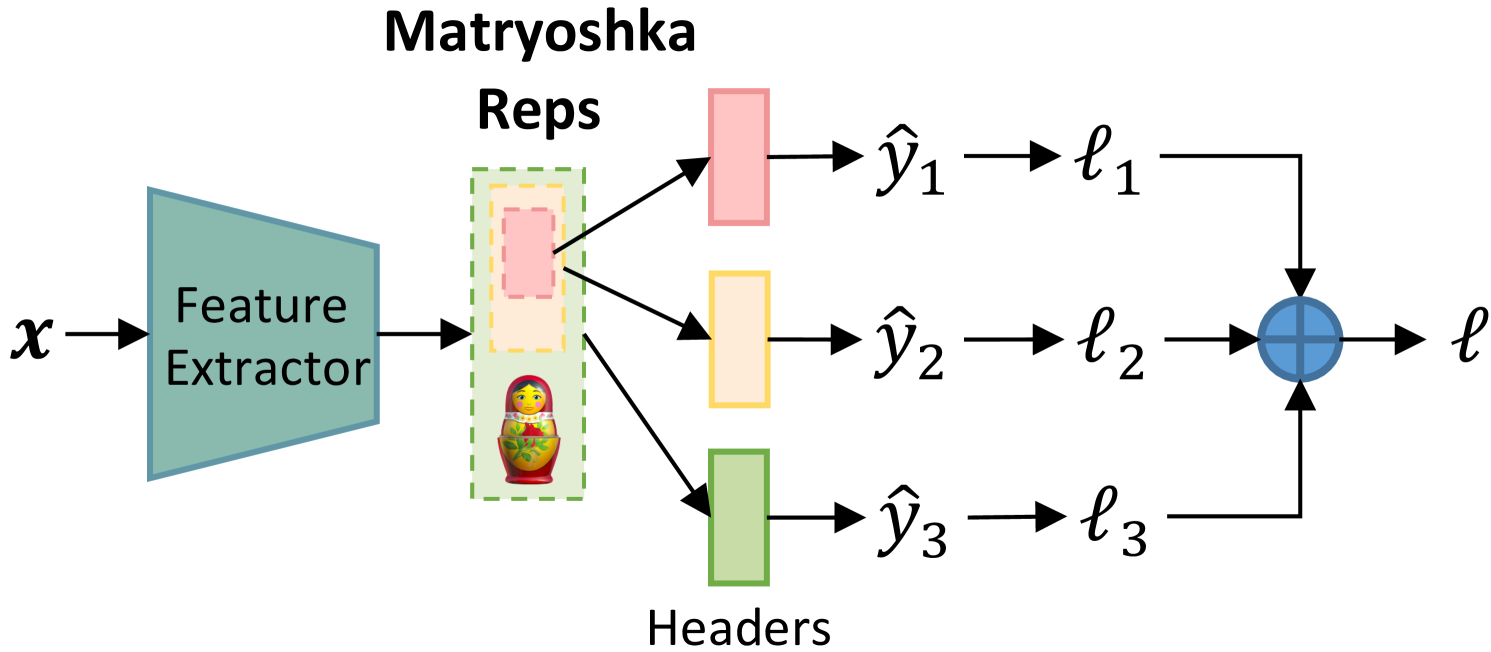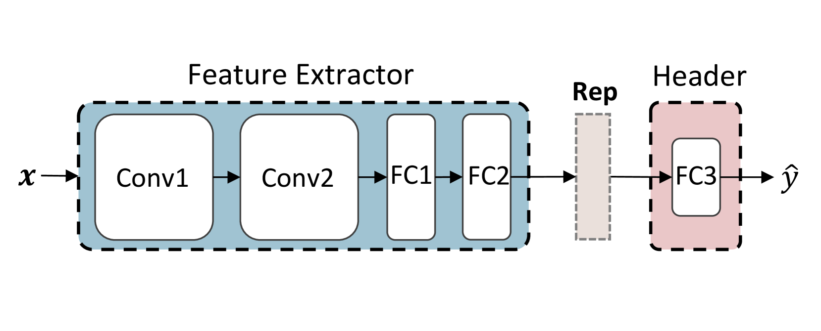</details> Figure 1: Left: Matryoshka Representation Learning. Right: Feature extractor and prediction header. Recently, Matryoshka Representation Learning (MRL) [21] has emerged to tailor representation dimensions based on the computational and storage costs required by downstream tasks to achieve a near-optimal trade-off between model performance and inference costs. As shown in Figure 1 (left), the representation extracted by the feature extractor is constructed to form Matryoshka Representations involving a series of embedded representations ranging from low-to-high dimensions and coarse-to-fine granularities. Each of them is processed by a single output layer for calculating loss, and the sum of losses from all branches is used to update model parameters. This design is inspired by the insight that people often first perceive the coarse aspect of a target before observing the details, with multi-perspective observations enhancing understanding. Inspired by MRL, we address the aforementioned limitations of MHeteroFL by proposing the Fed erated model heterogeneous M atryoshka R epresentation L earning (FedMRL) approach for supervised learning tasks. For each client, a shared global auxiliary homogeneous small model is added to interact with its heterogeneous local model. Both two models consist of a feature extractor and a prediction header, as depicted in Figure 1 (right). FedMRL has two key design innovations. (1) Adaptive Representation Fusion: for each local data sample, the feature extractors of the two local models extract generalized and personalized representations, respectively. The two representations are spliced and then mapped to a fused representation by a lightweight personalized representation projector adapting to local non-IID data. (2) Multi-Granularity Representation Learning: the fused representation is used to construct Matryoshka Representations involving multi-dimension and multi-granularity embedded representations, which are processed by the prediction headers of the two models, respectively. The sum of their losses is used to update all models, which enhances the model learning capability owing to multi-perspective representation learning. The personalized multi-granularity MRL enhances representation knowledge interaction between the homogeneous global model and the heterogeneous client local model. Each client’s local model and data are not exposed during training for privacy-preservation. The server and clients only transmit the small homogeneous models, thereby incurring low communication costs. Each client only trains a small homogeneous model and a lightweight representation projector in addition, incurring low extra computational costs. We theoretically derive the $\mathcal{O}(1/T)$ non-convex convergence rate of FedMRL and verify that it can converge over time. Experiments on benchmark datasets comparing FedMRL against seven state-of-the-art baselines demonstrate its superiority. It improves model accuracy by up to $8.48\%$ and $24.94\%$ over the best baseline and the best same-category baseline, while incurring lower communication and computation costs. 2 Related Work Existing MHeteroFL works can be divided into the following four categories. MHeteroFL with Adaptive Subnets. These methods [3, 4, 5, 11, 14, 56, 64] construct heterogeneous local subnets of the global model by parameter pruning or special designs to match with each client’s local system resources. The server aggregates heterogeneous local subnets wise parameters to generate a new global model. In cases where clients hold black-box local models with heterogeneous structures not derived from a common global model, the server is unable to aggregate them. MHeteroFL with Knowledge Distillation. These methods [6, 8, 9, 15, 16, 17, 22, 23, 25, 27, 30, 32, 35, 36, 42, 57, 59] often perform knowledge distillation on heterogeneous client models by leveraging a public dataset with the same data distribution as the learning task. In practice, such a suitable public dataset can be hard to find. Others [12, 60, 61, 63] train a generator to synthesize a shared dataset to deal with this issue. However, this incurs high training costs. The rest (FD [19], FedProto [41] and others [1, 2, 13, 49, 58]) share the intermediate information of client local data for knowledge fusion. MHeteroFL with Model Split. These methods split models into feature extractors and predictors. Some [7, 10, 31, 33] share homogeneous feature extractors across clients and personalize predictors, while others (LG-FedAvg [24] and [18, 26]) do the opposite. Such methods expose part of the local model structures, which might not be acceptable if the models are proprietary IPs of the clients. MHeteroFL with Mutual Learning. These methods (FedAPEN [34], FML [38], FedKD [43] and others [28]) add a shared global homogeneous small model on top of each client’s heterogeneous local model. For each local data sample, the distance of the outputs from these two models is used as the mutual loss to update model parameters. Nevertheless, the mutual loss only transfers limited knowledge between the two models, resulting in model performance bottlenecks. The proposed FedMRL approach further optimizes mutual learning-based MHeteroFL by enhancing the knowledge transfer between the server and client models. It achieves personalized adaptive representation fusion and multi-perspective representation learning, thereby facilitating more knowledge interaction across the two models and improving model performance. 3 The Proposed FedMRL Approach FedMRL aims to tackle data, system, and model heterogeneity in supervised learning tasks, where a central FL server coordinates $N$ FL clients to train heterogeneous local models. The server maintains a global homogeneous small model $\mathcal{G}(\theta)$ shared by all clients. Figure 2 depicts its workflow Algorithm 1 in Appendix A describes the FedMRL algorithm.: 1. In each communication round, $K$ clients participate in FL (i.e., the client participant rate $C=K/N$ ). The global homogeneous small model $\mathcal{G}(\theta)$ is broadcast to them. 1. Each client $k$ holds a heterogeneous local model $\mathcal{F}_{k}(\omega_{k})$ ( $\mathcal{F}_{k}(·)$ is the heterogeneous model structure, and $\omega_{k}$ are personalized model parameters). Client $k$ simultaneously trains the heterogeneous local model and the global homogeneous small model on local non-IID data $D_{k}$ ( $D_{k}$ follows the non-IID distribution $P_{k}$ ) via personalized Matryoshka Representations Learning with a personalized representation projector $\mathcal{P}_{k}(\varphi_{k})$ . 1. The updated homogeneous small models are uploaded to the server for aggregation to produce a new global model for knowledge fusion across heterogeneous clients. The objective of FedMRL is to minimize the sum of the loss from the combined models ( $\mathcal{W}_{k}(w_{k})=(\mathcal{G}(\theta)\circ\mathcal{F}_{k}(\omega_{k})|% \mathcal{P}_{k}(\varphi_{k}))$ ) on all clients, i.e., $$ \min_{\theta,\omega_{0,\ldots,N-1}}\sum_{k=0}^{N-1}\ell\left(\mathcal{W}_{k}% \left(D_{k};\left(\theta\circ\omega_{k}\mid\varphi_{k}\right)\right)\right). \tag{1} $$ These steps repeat until each client’s model converges. After FL training, a client uses its local combined model without the global header for inference. Appendix C.3 provides experimental evidence for inference model selection. <details> <summary>x3.png Details</summary>  ### Visual Description ## Diagram: Federated Learning Architecture with Local and Global Model Aggregation ### Overview The diagram illustrates a federated learning system where multiple clients (e.g., Client 1) train local homogeneous models on their data, which are aggregated into a global model on a server. The client-side workflow includes input processing, representation extraction, projection, and loss calculation for model inference. Key components include local homogeneous models, a global model, extractors, projectors, and Matryoshka representations. --- ### Components/Axes #### Server-Side Components 1. **Local Homogeneous Models**: - **Model 1**: Green block labeled `g(θ₁)`. - **Model 2**: Blue block labeled `g(θ₂)`. - **Model 3**: Beige block labeled `g(θ₃)`. 2. **Global Homogeneous Model**: Purple block labeled `g(θ)`, formed by aggregating local models. 3. **Flow**: Arrows indicate aggregation (`+`) from local models to the global model. #### Client-Side Components (Client 1) 1. **Input**: Image of a panda labeled `Input x_i`. 2. **Homo. Extractor**: Green block labeled `g_ex(θ_ex)`. 3. **Hetero. Extractor**: Yellow block labeled `F₁_ex(ω₁_ex)`. 4. **Representations**: - **Rep1**: Green block labeled `R_i^g`. - **Rep2**: Yellow block labeled `R_i^F1`. 5. **Projection**: Purple block labeled `P₁(φ₁)`. 6. **Matryoshka Reps**: Purple block with nested doll icon. 7. **Headers**: - **Header1**: Green block labeled `g_hd(θ_hd)`. - **Header2**: Yellow block labeled `F₁_hd(ω₁_hd)`. 8. **Outputs**: - **Output 1**: `ŷ_i^g` (green arrow). - **Output 2**: `ŷ_i^F1` (yellow arrow). 9. **Loss Functions**: - **Loss 1**: Blue arrow labeled `Loss` (global model). - **Loss 2**: Blue arrow labeled `Loss` (heterogeneous model). 10. **Model Inference**: Gray arrow labeled `Model Inference`. --- ### Detailed Analysis #### Server-Side - **Local Models**: Three distinct local homogeneous models (`g(θ₁)`, `g(θ₂)`, `g(θ₃)`) are trained independently on client data. - **Global Model**: Aggregated from local models via summation (`+`), resulting in `g(θ)`. #### Client-Side 1. **Input Processing**: - The panda image (`x_i`) is processed by two extractors: - **Homo. Extractor**: Generates homogeneous representation `R_i^g`. - **Hetero. Extractor**: Generates heterogeneous representation `R_i^F1`. 2. **Representation Splicing**: - `R_i^g` and `R_i^F1` are spliced into a combined representation `R_i`. 3. **Projection**: - Combined representation `R_i` is projected via `P₁(φ₁)` into a latent space. 4. **Matryoshka Reps**: - Nested representations (`Ũ_i`, `Ũ_i^F1`) are derived, likely for hierarchical feature learning. 5. **Headers**: - **Header1**: Processes `Ũ_i` via `g_hd(θ_hd)`. - **Header2**: Processes `Ũ_i^F1` via `F₁_hd(ω₁_hd)`. 6. **Loss Calculation**: - **Loss 1**: Measures discrepancy between `ŷ_i^g` and true label `y_i`. - **Loss 2**: Measures discrepancy between `ŷ_i^F1` and true label `y_i`. --- ### Key Observations 1. **Model Heterogeneity**: The system handles both homogeneous (`g(θ)`) and heterogeneous (`F₁(ω)`) feature extractors. 2. **Matryoshka Reps**: Suggests a nested representation strategy, possibly for multi-task learning or robustness. 3. **Loss Functions**: Dual loss objectives for global and task-specific model refinement. 4. **Color Coding**: - Green: Homogeneous components. - Blue: Server-side aggregation. - Yellow: Heterogeneous components. - Purple: Projection and Matryoshka representations. --- ### Interpretation This architecture demonstrates a hybrid federated learning approach: - **Local Training**: Clients train task-specific models (`g(θ₁)`, `g(θ₂)`, `g(θ₃)`) on their data. - **Global Aggregation**: Server combines local models into a unified `g(θ)`. - **Client-Side Personalization**: Matryoshka representations (`Ũ_i`, `Ũ_i^F1`) allow adaptation to individual client data distributions while leveraging global knowledge. - **Dual Objectives**: Loss 1 optimizes global model accuracy, while Loss 2 ensures task-specific performance via heterogeneous extractors. The use of Matryoshka Reps implies a focus on hierarchical feature learning, enabling the model to capture both general (global) and client-specific (local) patterns. This design balances personalization and generalization, critical for privacy-preserving federated learning. </details> Figure 2: The workflow of FedMRL. 3.1 Adaptive Representation Fusion We denote client $k$ ’s heterogeneous local model feature extractor as $\mathcal{F}_{k}^{ex}(\omega_{k}^{ex})$ , and prediction header as $\mathcal{F}_{k}^{hd}(\omega_{k}^{hd})$ . We denote the homogeneous global model feature extractor as $\mathcal{G}^{ex}(\theta^{ex})$ and prediction header as $\mathcal{G}^{hd}(\theta^{hd})$ . Client $k$ ’s local personalized representation projector is denoted as $\mathcal{P}_{k}(\varphi_{k})$ . In the $t$ -th communication round, client $k$ inputs its local data sample $(\boldsymbol{x}_{i},y_{i})∈ D_{k}$ into the two feature extractors to extract generalized and personalized representations as: $$ \boldsymbol{\mathcal{R}}_{i}^{\mathcal{G}}=\ \mathcal{G}^{ex}({\boldsymbol{x}_% {i};\theta}^{ex,t-1}),\boldsymbol{\mathcal{R}}_{i}^{\mathcal{F}_{k}}=\ % \mathcal{F}_{k}^{ex}(\boldsymbol{x}_{i};\omega_{k}^{ex,t-1}). \tag{2} $$ The two extracted representations $\boldsymbol{\mathcal{R}}_{i}^{\mathcal{G}}∈\mathbb{R}^{d_{1}}$ and $\boldsymbol{\mathcal{R}}_{i}^{\mathcal{F}_{k}}∈\mathbb{R}^{d_{2}}$ are spliced as: $$ \boldsymbol{\mathcal{R}}_{i}=\boldsymbol{\mathcal{R}}_{i}^{\mathcal{G}}\circ% \boldsymbol{\mathcal{R}}_{i}^{\mathcal{F}_{k}}. \tag{3} $$ Then, the spliced representation is mapped into a fused representation by the lightweight representation projector $\mathcal{P}_{k}(\varphi_{k}^{t-1})$ as: $$ {\widetilde{\boldsymbol{\mathcal{R}}}}_{i}=\mathcal{P}_{k}(\boldsymbol{% \mathcal{R}}_{i}{;\varphi}_{k}^{t-1}), \tag{4} $$ where the projector can be a one-layer linear model or multi-layer perceptron. The fused representation ${\widetilde{\boldsymbol{\mathcal{R}}}}_{i}$ contains both generalized and personalized feature information. It has the same dimension as the client’s local heterogeneous model representation $\mathbb{R}^{d_{2}}$ , which ensures the representation dimension $\mathbb{R}^{d_{2}}$ and the client local heterogeneous model header parameter dimension $\mathbb{R}^{d_{2}× L}$ ( $L$ is the label dimension) match. The representation projector can be updated as the two models are being trained on local non-IID data. Hence, it achieves personalized representation fusion adaptive to local data distributions. Splicing the representations extracted by two feature extractors can keep the relative semantic space positions of the generalized and personalized representations, benefiting the construction of multi-granularity Matryoshka Representations. Owing to representation splicing, the representation dimensions of the two feature extractors can be different (i.e., $d_{1}≤ d_{2}$ ). Therefore, we can vary the representation dimension of the small homogeneous global model to improve the trade-off among model performance, storage requirement and communication costs. In addition, each client’s local model is treated as a black box by the FL server. When the server broadcasts the global homogeneous small model to the clients, each client can adjust the linear layer dimension of the representation projector to align it with the dimension of the spliced representation. In this way, different clients may hold different representation projectors. When a new model-agnostic client joins in FedMRL, it can adjust its representation projector structure for local model training. Therefore, FedMRL can accommodate FL clients owning local models with diverse structures. 3.2 Multi-Granular Representation Learning To construct multi-dimensional and multi-granular Matryoshka Representations, we further extract a low-dimension coarse-granularity representation ${\widetilde{\boldsymbol{\mathcal{R}}}}_{i}^{lc}$ and a high-dimension fine-granularity representation ${\widetilde{\boldsymbol{\mathcal{R}}}}_{i}^{hf}$ from the fused representation ${\widetilde{\boldsymbol{\mathcal{R}}}}_{i}$ . They align with the representation dimensions $\{\mathbb{R}^{d_{1}},\mathbb{R}^{d_{2}}\}$ of two feature extractors for matching the parameter dimensions $\{\mathbb{R}^{d_{1}× L},\mathbb{R}^{d_{2}× L}\}$ of the two prediction headers, $$ {\widetilde{\boldsymbol{\mathcal{R}}}}_{i}^{lc}={{\widetilde{\boldsymbol{% \mathcal{R}}}}_{i}}^{1:d_{1}},{\widetilde{\boldsymbol{\mathcal{R}}}}_{i}^{hf}=% {{\widetilde{\boldsymbol{\mathcal{R}}}}_{i}}^{1:d_{2}}. \tag{5} $$ The embedded low-dimension coarse-granularity representation ${\widetilde{\boldsymbol{\mathcal{R}}}}_{i}^{lc}∈\mathbb{R}^{d_{1}}$ incorporates coarse generalized and personalized feature information. It is learned by the global homogeneous model header $\mathcal{G}^{hd}(\theta^{hd,t-1})$ (parameter space: $\mathbb{R}^{d_{1}× L}$ ) with generalized prediction information to produce: $$ {\hat{{y}}}_{i}^{\mathcal{G}}=\mathcal{G}^{hd}({\widetilde{\boldsymbol{% \mathcal{R}}}}_{i}^{lc};\theta^{hd,t-1}). \tag{6} $$ The embedded high-dimension fine-granularity representation ${\widetilde{\boldsymbol{\mathcal{R}}}}_{i}^{hf}∈\mathbb{R}^{d_{2}}$ carries finer generalized and personalized feature information, which is further processed by the heterogeneous local model header $\mathcal{F}_{k}^{hd}(\omega_{k}^{hd,t-1})$ (parameter space: $\mathbb{R}^{d_{2}× L}$ ) with personalized prediction information to generate: $$ {\hat{{y}}}_{i}^{\mathcal{F}_{k}}=\mathcal{F}_{k}^{hd}({\widetilde{\boldsymbol% {\mathcal{R}}}}_{i}^{hf};\omega_{k}^{hd,t-1}). \tag{7} $$ We compute the losses $\ell$ (e.g., cross-entropy loss [62]) between the two outputs and the label $y_{i}$ as: $$ \ell_{i}^{\mathcal{G}}=\ell({\hat{{y}}}_{i}^{\mathcal{G}},y_{i}),\ \ell_{i}^{% \mathcal{F}_{k}}=\ell({\hat{{y}}}_{i}^{\mathcal{F}_{k}},y_{i}). \tag{8} $$ Then, the losses of the two branches are weighted by their importance $m_{i}^{\mathcal{G}}$ and $m_{i}^{\mathcal{F}_{k}}$ and summed as: $$ \ell_{i}=m_{i}^{\mathcal{G}}\cdot\ell_{i}^{\mathcal{G}}+m_{i}^{\mathcal{F}_{k}% }\cdot\ell_{i}^{\mathcal{F}_{k}}. \tag{9} $$ We set $m_{i}^{\mathcal{G}}=m_{i}^{\mathcal{F}_{k}}=1$ by default to make the two models contribute equally to model performance. The complete loss $\ell_{i}$ is used to simultaneously update the homogeneous global small model, the heterogeneous client local model, and the representation projector via gradient descent: $$ \displaystyle\theta_{k}^{t} \displaystyle\leftarrow\theta^{t-1}-\eta_{\theta}\nabla\ell_{i}, \displaystyle\omega_{k}^{t} \displaystyle\leftarrow\omega_{k}^{t-1}-\eta_{\omega}\nabla\ell_{i}, \displaystyle\varphi_{k}^{t} \displaystyle\leftarrow\varphi_{k}^{t-1}-\eta_{\varphi}\nabla\ell_{i}, \tag{10} $$ where $\eta_{\theta},\eta_{\omega},\ \eta_{\varphi}$ are the learning rates of the homogeneous global small model, the heterogeneous local model and the representation projector. We set $\eta_{\theta}=\eta_{\omega}=\ \eta_{\varphi}$ by default to ensure stable model convergence. In this way, the generalized and personalized fused representation is learned from multiple perspectives, thereby improving model learning capability. 4 Convergence Analysis Based on notations, assumptions and proofs in Appendix B, we analyse the convergence of FedMRL. **Lemma 1** *Local Training. Given Assumptions 1 and 2, the loss of an arbitrary client’s local model $w$ in local training round $(t+1)$ is bounded by: $$ \mathbb{E}[\mathcal{L}_{(t+1)E}]\leq\mathcal{L}_{tE+0}+(\frac{L_{1}\eta^{2}}{2% }-\eta)\sum_{e=0}^{E}\|\nabla\mathcal{L}_{tE+e}\|_{2}^{2}+\frac{L_{1}E\eta^{2}% \sigma^{2}}{2}. \tag{11} $$* **Lemma 2** *Model Aggregation. Given Assumptions 2 and 3, after local training round $(t+1)$ , a client’s loss before and after receiving the updated global homogeneous small models is bounded by: $$ \mathbb{E}[\mathcal{L}_{(t+1)E+0}]\leq\mathbb{E}[\mathcal{L}_{tE+1}]+{\eta% \delta}^{2}. \tag{12} $$* **Theorem 1** *One Complete Round of FL. Given the above lemmas, for any client, after receiving the updated global homogeneous small model, we have: $$ \mathbb{E}[\mathcal{L}_{(t+1)E+0}]\leq\mathcal{L}_{tE+0}+(\frac{L_{1}\eta^{2}}% {2}-\eta)\sum_{e=0}^{E}\|\nabla\mathcal{L}_{tE+e}\|_{2}^{2}+\frac{L_{1}E\eta^{% 2}\sigma^{2}}{2}+\eta\delta^{2}. \tag{13} $$* **Theorem 2** *Non-convex Convergence Rate of FedMRL. Given Theorem 1, for any client and an arbitrary constant $\epsilon>0$ , the following holds: $$ \displaystyle\frac{1}{T}\sum_{t=0}^{T-1}\sum_{e=0}^{E-1}\|\nabla\mathcal{L}_{% tE+e}\|_{2}^{2} \displaystyle\leq\frac{\frac{1}{T}\sum_{t=0}^{T-1}[\mathcal{L}_{tE+0}-\mathbb{% E}[\mathcal{L}_{(t+1)E+0}]]+\frac{L_{1}E\eta^{2}\sigma^{2}}{2}+\eta\delta^{2}}% {\eta-\frac{L_{1}\eta^{2}}{2}}<\epsilon, \displaystyle s.t. \displaystyle\eta<\frac{2(\epsilon-\delta^{2})}{L_{1}(\epsilon+E\sigma^{2})}. \tag{14} $$* Therefore, we conclude that any client’s local model can converge at a non-convex rate of $\epsilon\sim\mathcal{O}(1/T)$ in FedMRL if the learning rates of the homogeneous small model, the client local heterogeneous model and the personalized representation projector satisfy the above conditions. 5 Experimental Evaluation We implement FedMRL on Pytorch, and compare it with seven state-of-the-art MHeteroFL methods. The experiments are carried out over two benchmark supervised image classification datasets on $4$ NVIDIA GeForce 3090 GPUs (24GB Memory). Codes are available in supplemental materials. 5.1 Experiment Setup Datasets. The benchmark datasets adopted are CIFAR-10 and CIFAR-100 https://www.cs.toronto.edu/%7Ekriz/cifar.html [20], which are commonly used in FL image classification tasks for the evaluating existing MHeteroFL algorithms. CIFAR-10 has $60,000$ $32× 32$ colour images across $10$ classes, with $50,000$ for training and $10,000$ for testing. CIFAR-100 has $60,000$ $32× 32$ colour images across $100$ classes, with $50,000$ for training and $10,000$ for testing. We follow [37] and [34] to construct two types of non-IID datasets. Each client’s non-IID data are further divided into a training set and a testing set with a ratio of $8:2$ . - Non-IID (Class): For CIFAR-10 with $10$ classes, we randomly assign $2$ classes to each FL client. For CIFAR-100 with $100$ classes, we randomly assign $10$ classes to each FL client. The fewer classes each client possesses, the higher the non-IIDness. 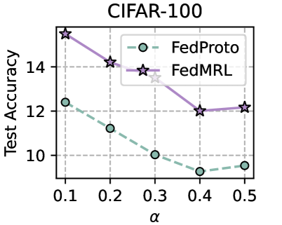- Non-IID (Dirichlet): To produce more sophisticated non-IID data settings, for each class of CIFAR-10/CIFAR-100, we use a Dirichlet( $\alpha$ ) function to adjust the ratio between the number of FL clients and the assigned data. A smaller $\alpha$ indicates more pronounced non-IIDness. Models. We evaluate MHeteroFL algorithms under model-homogeneous and heterogeneous FL scenarios. FedMRL ’s representation projector is a one-layer linear model (parameter space: $\mathbb{R}^{d2×(d_{1}+d_{2})}$ ). - Model-Homogeneous FL: All clients train CNN-1 in Table 2 (Appendix C.1). The homogeneous global small models in FML and FedKD are also CNN-1. The extra homogeneous global small model in FedMRL is CNN-1 with a smaller representation dimension $d_{1}$ (i.e., the penultimate linear layer dimension) than the CNN-1 model’s representation dimension $d_{2}$ , $d_{1}≤ d_{2}$ . - Model-Heterogeneous FL: The $5$ heterogeneous models {CNN-1, $...$ , CNN-5} in Table 2 (Appendix C.1) are evenly distributed among FL clients. The homogeneous global small models in FML and FedKD are the smallest CNN-5 models. The homogeneous global small model in FedMRL is the smallest CNN-5 with a reduced representation dimension $d_{1}$ compared with the CNN-5 model representation dimension $d_{2}$ , i.e., $d_{1}≤ d_{2}$ . Comparison Baselines. We compare FedMRL with state-of-the-art algorithms belonging to the following three categories of MHeteroFL methods: - Standalone. Each client trains its heterogeneous local model only with its local data. - Knowledge Distillation Without Public Data: FD [19] and FedProto [41]. - Model Split: LG-FedAvg [24]. - Mutual Learning: FML [38], FedKD [43] and FedAPEN [34]. Evaluation Metrics. We evaluate MHeteroFL algorithms from the following three aspects: - Model Accuracy. We record the test accuracy of each client’s model in each round, and compute the average test accuracy. - Communication Cost. We compute the number of parameters sent between the server and one client in one communication round, and record the required rounds for reaching the target average accuracy. The overall communication cost of one client for target average accuracy is the product between the cost per round and the number of rounds. - Computation Overhead. We compute the computation FLOPs of one client in one communication round, and record the required communication rounds for reaching the target average accuracy. The overall computation overall for one client achieving the target average accuracy is the product between the FLOPs per round and the number of rounds. 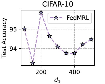Training Strategy. We search optimal FL hyperparameters and unique hyperparameters for all MHeteroFL algorithms. For FL hyperparameters, we test MHeteroFL algorithms with a $\{64,128,256,512\}$ batch size, $\{1,10\}$ epochs, $T=\{100,500\}$ communication rounds and an SGD optimizer with a $0.01$ learning rate. The unique hyperparameter of FedMRL is the representation dimension $d_{1}$ of the homogeneous global small model, we vary $d_{1}=\{100,\ 150,...,500\}$ to obtain the best-performing FedMRL. 5.2 Results and Discussion We design three FL settings with different numbers of clients ( $N$ ) and client participation rates ( $C$ ): ( $N=10,C=100\%$ ), ( $N=50,C=20\%$ ), ( $N=100,C=10\%$ ) for both model-homogeneous and model-heterogeneous FL scenarios. 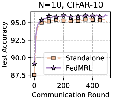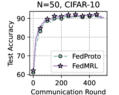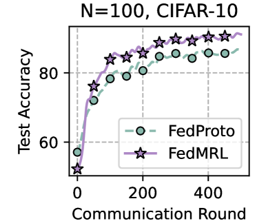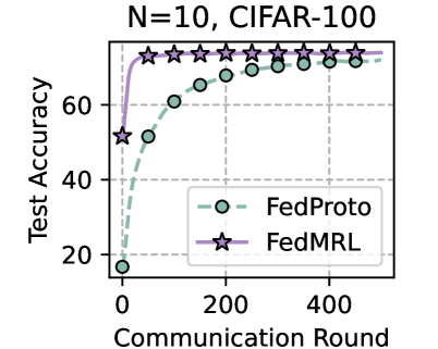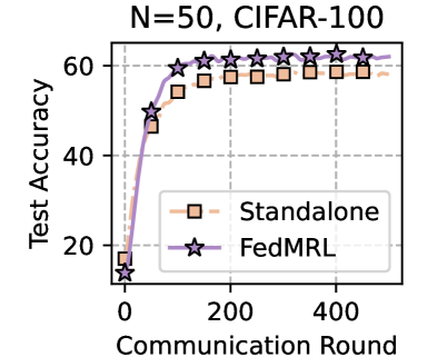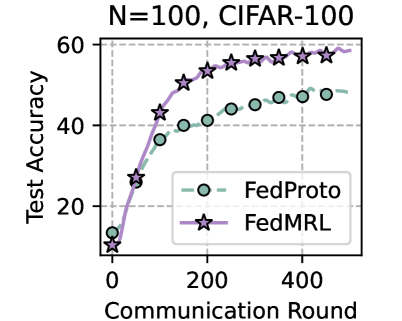5.2.1 Average Test Accuracy Table 1 and Table 3 (Appendix C.2) show that FedMRL consistently outperforms all baselines under both model-heterogeneous or homogeneous settings. It achieves up to a $8.48\%$ improvement in average test accuracy compared with the best baseline under each setting. Furthermore, it achieves up to a $24.94\%$ average test accuracy improvement than the best same-category (i.e., mutual learning-based MHeteroFL) baseline under each setting. These results demonstrate the superiority of FedMRL in model performance owing to its adaptive personalized representation fusion and multi-granularity representation learning capabilities. Figure 3 (left six) shows that FedMRL consistently achieves faster convergence speed and higher average test accuracy than the best baseline under each setting. 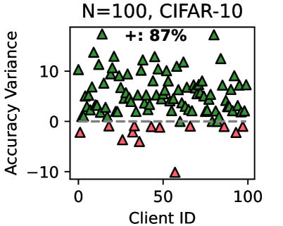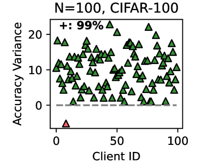5.2.2 Individual Client Test Accuracy Figure 3 (right two) shows the difference between the test accuracy achieved by FedMRL vs. the best-performing baseline FedProto (i.e., FedMRL - FedProto) under ( $N=100,C=10\%$ ) for each individual client. It can be observed that $87\%$ and $99\%$ of all clients achieve better performance under FedMRL than under FedProto on CIFAR-10 and CIFAR-100, respectively. This demonstrates that FedMRL possesses stronger personalization capability than FedProto owing to its adaptive personalized multi-granularity representation learning design. Table 1: Average test accuracy (%) in model-heterogeneous FL. | FL Setting Method Standalone | N=10, C=100% CIFAR-10 96.53 | N=50, C=20% CIFAR-100 72.53 | N=100, C=10% CIFAR-10 95.14 | CIFAR-100 62.71 | CIFAR-10 91.97 | CIFAR-100 53.04 | | --- | --- | --- | --- | --- | --- | --- | | LG-FedAvg [24] | 96.30 | 72.20 | 94.83 | 60.95 | 91.27 | 45.83 | | FD [19] | 96.21 | - | - | - | - | - | | FedProto [41] | 96.51 | 72.59 | 95.48 | 62.69 | 92.49 | 53.67 | | FML [38] | 30.48 | 16.84 | - | 21.96 | - | 15.21 | | FedKD [43] | 80.20 | 53.23 | 77.37 | 44.27 | 73.21 | 37.21 | | FedAPEN [34] | - | - | - | - | - | - | | FedMRL | 96.63 | 74.37 | 95.70 | 66.04 | 95.85 | 62.15 | | FedMRL -Best B. | 0.10 | 1.78 | 0.22 | 3.33 | 3.36 | 8.48 | | FedMRL -Best S.C.B. | 16.43 | 21.14 | 18.33 | 21.77 | 22.64 | 24.94 | “-”: failing to converge. “ ”: the best MHeteroFL method. “ Best B.”: the best baseline. “ Best S.C.B.”: the best same-category (mutual learning-based MHeteroFL) baseline. The underscored values denote the largest accuracy improvement of FedMRL across $6$ settings. <details> <summary>x4.png Details</summary>  ### Visual Description ## Line Chart: N=10, CIFAR-10 Test Accuracy vs. Communication Rounds ### Overview The chart compares the test accuracy of two machine learning methods ("Standalone" and "FedMRL") over communication rounds during training on the CIFAR-10 dataset with a sample size of N=10. Both methods show rapid convergence to high accuracy, with FedMRL achieving slightly better initial performance but both plateauing at ~95% accuracy after 200 rounds. ### Components/Axes - **X-axis**: "Communication Round" (0 to 400, increments of 200) - **Y-axis**: "Test Accuracy" (87.5% to 95%, increments of 2.5%) - **Legend**: - Orange squares: "Standalone" - Purple stars: "FedMRL" - **Title**: "N=10, CIFAR-10" (top center) - **Grid**: Dashed gray lines for reference ### Detailed Analysis 1. **Standalone (Orange Squares)**: - Starts at **~87.5%** accuracy at 0 rounds. - Sharp increase to **~95%** by 200 rounds. - Remains stable at ~95% through 400 rounds. - Error bars (if present) suggest minor variance (~±0.5%). 2. **FedMRL (Purple Stars)**: - Begins at **~88%** accuracy at 0 rounds. - Reaches **~95%** by 200 rounds, matching Standalone. - Maintains ~95% accuracy through 400 rounds. - Error bars (if present) suggest similar variance to Standalone. ### Key Observations - Both methods converge to identical accuracy (~95%) after 200 rounds. - FedMRL demonstrates a **~0.5% initial advantage** over Standalone. - No significant divergence between methods after 200 rounds. - Accuracy plateaus suggest diminishing returns beyond 200 rounds. ### Interpretation The data indicates that **FedMRL** outperforms "Standalone" in early training stages but both methods achieve equivalent performance by 200 communication rounds. This suggests that: 1. **Communication efficiency**: FedMRL’s distributed approach provides faster initial gains. 2. **Convergence behavior**: Both methods stabilize at similar accuracy, implying that CIFAR-10’s complexity is manageable with either approach given sufficient rounds. 3. **Diminishing returns**: Additional rounds beyond 200 yield negligible improvements, highlighting potential optimization opportunities for training efficiency. The chart underscores the trade-off between initial performance and long-term stability, with FedMRL offering a slight edge for rapid deployment scenarios. </details> <details> <summary>x5.png Details</summary>  ### Visual Description ## Line Chart: Test Accuracy vs Communication Rounds (N=50, CIFAR-10) ### Overview The chart compares the test accuracy of two federated learning algorithms, **FedProto** and **FedMRL**, over communication rounds on the CIFAR-10 dataset with 50 clients. Both models show improvement in accuracy as communication rounds increase, but **FedMRL** consistently outperforms **FedProto** after 200 rounds. ### Components/Axes - **X-axis**: Communication Rounds (0, 200, 400) - **Y-axis**: Test Accuracy (60–90%) - **Legend**: - **FedProto**: Green circles (dashed line) - **FedMRL**: Purple stars (solid line) - **Title**: "N=50, CIFAR-10" (top center) ### Detailed Analysis 1. **FedProto** (green circles): - Starts at ~60% accuracy at 0 rounds. - Sharp increase to ~85% by 200 rounds. - Plateaus near 90% after 200 rounds with minimal further improvement. - Final accuracy at 400 rounds: ~90% (uncertainty: ±1%). 2. **FedMRL** (purple stars): - Begins slightly below FedProto (~62% at 0 rounds). - Accelerates faster, surpassing FedProto by 200 rounds (~88% vs. ~85%). - Reaches ~92% accuracy by 400 rounds, maintaining a ~2% lead over FedProto. - Final accuracy at 400 rounds: ~92% (uncertainty: ±1%). ### Key Observations - **Convergence Speed**: FedMRL converges faster, achieving higher accuracy earlier. - **Plateauing**: FedProto’s accuracy stabilizes after 200 rounds, while FedMRL continues improving. - **Performance Gap**: By 400 rounds, FedMRL outperforms FedProto by ~2%, suggesting superior optimization or robustness. ### Interpretation The data demonstrates that **FedMRL** is more effective for federated learning on CIFAR-10 with 50 clients, likely due to better handling of non-IID data or improved aggregation mechanisms. The plateau in FedProto’s performance highlights potential limitations in its convergence strategy. The ~2% accuracy gap at 400 rounds underscores the importance of algorithmic design in federated settings, where communication efficiency and model robustness are critical. The consistent upward trend for FedMRL suggests it scales better with increased communication rounds, making it preferable for resource-constrained environments. </details> <details> <summary>x6.png Details</summary>  ### Visual Description ## Line Graph: Test Accuracy vs Communication Rounds (N=100, CIFAR-10) ### Overview The graph compares the test accuracy of two federated learning algorithms, **FedProto** and **FedMRL**, over 400 communication rounds on the CIFAR-10 dataset with a sample size of N=100. Both algorithms show increasing accuracy, with FedMRL consistently outperforming FedProto after ~100 rounds. ### Components/Axes - **X-axis**: Communication Rounds (0 to 400, increments of 100). - **Y-axis**: Test Accuracy (50% to 100%, increments of 10%). - **Legend**: - **FedProto**: Green circles (dashed line). - **FedMRL**: Purple stars (solid line). - **Title**: "N=100, CIFAR-10" (top center). ### Detailed Analysis 1. **FedProto (Green Circles)**: - Starts at ~55% accuracy at 0 rounds. - Increases steadily to ~88% by 400 rounds. - Key data points: - 0 rounds: ~55% - 100 rounds: ~75% - 200 rounds: ~82% - 300 rounds: ~85% - 400 rounds: ~88% 2. **FedMRL (Purple Stars)**: - Begins at ~50% accuracy at 0 rounds. - Outperforms FedProto after ~100 rounds, reaching ~90% by 400 rounds. - Key data points: - 0 rounds: ~50% - 100 rounds: ~78% - 200 rounds: ~85% - 300 rounds: ~88% - 400 rounds: ~90% ### Key Observations - **Convergence**: Both algorithms plateau near 85–90% accuracy after 300 rounds, suggesting diminishing returns. - **Performance Gap**: FedMRL achieves ~5–7% higher accuracy than FedProto by 400 rounds. - **Early Growth**: FedMRL’s accuracy rises more sharply in the first 100 rounds compared to FedProto. ### Interpretation The graph demonstrates that **FedMRL** is more effective than **FedProto** for this CIFAR-10 setup, particularly in later communication rounds. The convergence at higher rounds implies that both methods reach near-optimal performance with ~300 rounds, but FedMRL’s superior efficiency or model architecture allows it to maintain a slight edge. This could indicate better handling of non-IID data or improved aggregation strategies in FedMRL. The plateau suggests that further rounds beyond 300 yield minimal gains, highlighting a potential optimization target for communication efficiency. </details> <details> <summary>x7.png Details</summary>  ### Visual Description ## Scatter Plot: Accuracy Variance Across Clients (CIFAR-10 Dataset) ### Overview The image is a scatter plot visualizing the distribution of accuracy variance across 100 clients in the CIFAR-10 dataset. Data points are represented by colored triangles, with a dashed horizontal line at 0 accuracy variance for reference. The plot highlights a significant imbalance between clients with positive and negative accuracy variance. ### Components/Axes - **X-axis**: Client ID (0 to 100, evenly spaced). - **Y-axis**: Accuracy Variance (-10 to 10, linear scale). - **Legend**: Located in the top-right corner. - Green triangles: "+: 87%" (positive accuracy variance). - Red triangles: "-: 13%" (negative accuracy variance). - **Dashed Line**: Horizontal line at y=0, separating positive and negative variance. ### Detailed Analysis - **Green Triangles (87%)**: - Majority clustered between y=0 and y=10, with a few outliers below y=0. - Spatial distribution: Concentrated in the upper half of the plot, indicating most clients have positive variance. - **Red Triangles (13%)**: - Primarily clustered between y=-10 and y=0, with one outlier above y=0. - Spatial distribution: Dominates the lower half of the plot, indicating most clients have negative variance. - **Dashed Line**: Acts as a baseline; 87% of data points (green) lie above it, while 13% (red) lie below. ### Key Observations 1. **Dominance of Positive Variance**: 87% of clients exhibit higher accuracy than the baseline (y=0), suggesting robust performance for most clients. 2. **Notable Outliers**: - A single red triangle (Client ID ~50) lies above y=0, indicating an exception in the negative variance group. - Several green triangles (Client IDs ~10, 30, 70) fall below y=0, showing exceptions in the positive variance group. 3. **Variability**: The spread of points (y=-10 to y=10) reflects significant client-to-client performance differences. ### Interpretation The data suggests that in the CIFAR-10 dataset with 100 clients: - **Model Robustness**: Most clients (87%) achieve higher accuracy than the baseline, possibly due to effective training or data distribution alignment. - **Performance Variability**: The 13% of clients with negative variance may indicate issues like overfitting, data scarcity, or misalignment with the global model. - **Outlier Implications**: The red triangle above y=0 and green triangles below y=0 highlight edge cases that warrant further investigation (e.g., data quality, client-specific biases). This visualization underscores the importance of client-level analysis in federated learning or distributed training scenarios, where performance disparities can impact overall system reliability. </details> <details> <summary>x8.png Details</summary>  ### Visual Description ## Line Graph: N=10, CIFAR-100 ### Overview The image is a line graph comparing the test accuracy of two federated learning algorithms, **FedProto** and **FedMRL**, over communication rounds on the CIFAR-100 dataset with N=10 clients. The y-axis represents test accuracy (%), and the x-axis represents communication rounds (0–400). Both algorithms show increasing accuracy with more rounds, but FedMRL consistently outperforms FedProto. --- ### Components/Axes - **Y-Axis**: "Test Accuracy" (%), scaled from 0 to 80 in increments of 20. - **X-Axis**: "Communication Round", scaled from 0 to 400 in increments of 200. - **Legend**: Located at the bottom-right corner. - **FedProto**: Dashed teal line with hollow circles (data points). - **FedMRL**: Solid purple line with star markers (data points). --- ### Detailed Analysis 1. **FedProto**: - Starts at **~15%** accuracy at 0 rounds. - Increases sharply to **~60%** by 200 rounds. - Plateaus near **~70%** by 400 rounds. - Data points: (0, ~15), (200, ~60), (400, ~70). 2. **FedMRL**: - Starts at **~55%** accuracy at 0 rounds. - Rises to **~75%** by 200 rounds. - Maintains **~75%** accuracy at 400 rounds. - Data points: (0, ~55), (200, ~75), (400, ~75). --- ### Key Observations - **FedMRL** achieves higher accuracy than **FedProto** at all communication rounds. - **FedProto** shows a steeper initial improvement but plateaus earlier. - Both algorithms converge near 400 rounds, but FedMRL retains a **~5% accuracy advantage**. - No outliers or anomalies; trends are smooth and consistent. --- ### Interpretation The graph demonstrates that **FedMRL** is more efficient and effective than **FedProto** for this task. FedMRL achieves higher accuracy with fewer communication rounds, suggesting superior model architecture or optimization. The convergence at 400 rounds implies that while FedProto improves significantly over time, FedMRL’s performance is more stable and robust. This could inform algorithm selection in resource-constrained federated learning scenarios. </details> <details> <summary>x9.png Details</summary>  ### Visual Description ## Line Graph: N=50, CIFAR-100 Test Accuracy vs. Communication Rounds ### Overview The image is a line graph comparing the test accuracy of two machine learning models ("Standalone" and "FedML") over communication rounds during training on the CIFAR-100 dataset with 50 clients. The y-axis represents test accuracy (0–60%), and the x-axis represents communication rounds (0–400). The graph includes a legend in the bottom-right corner and gridlines for reference. --- ### Components/Axes - **Title**: "N=50, CIFAR-100" (top-center). - **Y-Axis**: "Test Accuracy" (0–60%, labeled vertically on the left). - **X-Axis**: "Communication Round" (0–400, labeled horizontally at the bottom). - **Legend**: Located in the bottom-right corner, with: - **Orange squares**: "Standalone" model. - **Purple stars**: "FedML" model. - **Gridlines**: Dashed lines at x=0, 100, 200, 300, 400 and y=0, 20, 40, 60. --- ### Detailed Analysis 1. **Standalone Model (Orange Squares)**: - Starts at ~15% accuracy at 0 rounds. - Increases sharply to ~55% by 100 rounds. - Plateaus near 55% for subsequent rounds (200–400). 2. **FedML Model (Purple Stars)**: - Starts at ~10% accuracy at 0 rounds. - Rises steeply to surpass Standalone (~60%) by ~200 rounds. - Maintains ~60% accuracy for rounds 200–400. --- ### Key Observations - **Performance Divergence**: FedML outperforms Standalone after ~200 rounds, achieving higher accuracy with fewer rounds. - **Plateau Effect**: Both models plateau before 400 rounds, suggesting diminishing returns. - **Efficiency**: FedML reaches ~60% accuracy by ~200 rounds, while Standalone requires ~100 rounds to reach ~55%. --- ### Interpretation The data demonstrates that **FedML** is more efficient for distributed learning on CIFAR-100 with 50 clients, achieving higher accuracy with fewer communication rounds compared to the Standalone model. The plateau effect indicates that increasing rounds beyond ~200 provides minimal gains, likely due to model saturation or overfitting. This suggests FedML’s federated learning framework optimizes resource usage, making it preferable for large-scale, resource-constrained environments. The Standalone model’s slower convergence highlights the limitations of non-distributed training in such scenarios. </details> <details> <summary>x10.png Details</summary>  ### Visual Description ## Line Graph: Test Accuracy vs Communication Rounds (N=100, CIFAR-100) ### Overview The image is a line graph comparing the test accuracy of two federated learning algorithms, **FedProto** and **FedMRL**, over communication rounds on the CIFAR-100 dataset with 100 clients (N=100). The y-axis represents test accuracy (0–60%), and the x-axis represents communication rounds (0–400). Two data series are plotted: FedProto (dashed line with green circles) and FedMRL (solid line with purple stars). --- ### Components/Axes - **Title**: "N=100, CIFAR-100" (top center). - **Y-Axis**: "Test Accuracy" (0–60%, labeled vertically on the left). - **X-Axis**: "Communication Round" (0–400, labeled horizontally at the bottom). - **Legend**: Located at the bottom-right corner, with: - **FedProto**: Dashed green line with hollow green circles. - **FedMRL**: Solid purple line with filled purple stars. - **Grid**: Dashed gray grid lines for reference. --- ### Detailed Analysis #### FedProto (Green Dashed Line) - **Initial Value**: ~10% accuracy at 0 rounds. - **Trend**: Gradual increase to ~50% accuracy at 200 rounds, followed by a plateau near 50%. - **Key Points**: - 0 rounds: ~10%. - 100 rounds: ~35%. - 200 rounds: ~50%. - 400 rounds: ~50%. #### FedMRL (Purple Solid Line) - **Initial Value**: ~5% accuracy at 0 rounds. - **Trend**: Sharp rise to ~55% accuracy at 200 rounds, followed by stabilization near 55%. - **Key Points**: - 0 rounds: ~5%. - 100 rounds: ~45%. - 200 rounds: ~55%. - 400 rounds: ~55%. **Crossing Point**: The lines intersect at ~100 rounds, where FedMRL surpasses FedProto in accuracy. --- ### Key Observations 1. **Performance Gap**: FedMRL consistently outperforms FedProto after 100 rounds, achieving ~55% accuracy vs. FedProto’s ~50%. 2. **Diminishing Returns**: Both algorithms plateau after 200 rounds, suggesting limited gains from additional communication. 3. **Efficiency**: FedMRL achieves higher accuracy with fewer rounds (e.g., 55% at 200 rounds vs. FedProto’s 50%). 4. **Initial Disparity**: FedProto starts stronger (10% vs. 5% at 0 rounds), but FedMRL accelerates faster. --- ### Interpretation - **Algorithm Efficiency**: FedMRL’s superior performance indicates better optimization for communication efficiency, critical in resource-constrained federated learning scenarios. - **Plateau Implications**: The plateau at ~200 rounds suggests that further communication rounds yield minimal accuracy improvements, highlighting the importance of early-stage optimization. - **Trade-Off Analysis**: The crossing point at 100 rounds implies a trade-off between initial accuracy (FedProto) and long-term efficiency (FedMRL). FedMRL’s rapid convergence makes it preferable for scenarios prioritizing rapid deployment. **Uncertainties**: Values are approximate due to lack of error bars. The exact crossing point (100 rounds) is inferred from visual alignment, not explicit data points. </details> <details> <summary>x11.png Details</summary>  ### Visual Description ## Scatter Plot: N=100, CIFAR-100 ### Overview The image is a scatter plot visualizing the relationship between **Client ID** (x-axis) and **Accuracy Variance** (y-axis) for 100 clients. The plot uses green triangles to represent data points, with a single red triangle as an outlier. A dashed horizontal line at y=0 is present, and a legend indicates "+: 99%". ### Components/Axes - **X-axis (Client ID)**: Ranges from 0 to 100, labeled "Client ID". - **Y-axis (Accuracy Variance)**: Ranges from 0 to 20, labeled "Accuracy Variance". - **Legend**: Located in the top-right corner, with a green triangle labeled "+: 99%". - **Outlier**: A red triangle at (Client ID = 0, Accuracy Variance ≈ 0). ### Detailed Analysis - **Data Points**: - **Green Triangles**: Approximately 99% of the data points (as per the legend) are distributed across the plot. Most points cluster between y=0 and y=10, with some variability. A few points reach up to y=20. - **Red Triangle**: A single outlier at (0, 0), positioned at the bottom-left corner of the plot. - **Dashed Line**: A horizontal dashed line at y=0 separates the plot, likely indicating a baseline or threshold. ### Key Observations 1. **Outlier**: The red triangle at (0, 0) is the only data point with 0 accuracy variance, suggesting a significant deviation from the majority. 2. **Distribution**: Most clients (99%) exhibit accuracy variance between 0 and 20, with no clear upward or downward trend. 3. **Clustering**: Data points are densely packed in the lower half of the plot (y=0–10), with sparse points in the upper half (y=10–20). ### Interpretation - **Data Trends**: The majority of clients show moderate accuracy variance, indicating relatively consistent performance. The outlier (Client ID 0) may represent a unique case, such as a client with no data, a failed model, or an error in data collection. - **Legend Context**: The "+: 99%" label suggests that 99% of the data points meet a specific criterion (e.g., non-zero variance), but the exact threshold is not explicitly defined in the plot. - **Anomalies**: The red triangle’s position at (0, 0) raises questions about its validity. It could indicate a missing or corrupted dataset for Client ID 0, or a deliberate exclusion from the 99% majority. This plot highlights the variability in model performance across clients, with a critical outlier requiring further investigation. </details> Figure 3: Left six: average test accuracy vs. communication rounds. Right two: individual clients’ test accuracy (%) differences (FedMRL - FedProto). <details> <summary>x12.png Details</summary>  ### Visual Description ## Bar Chart: Communication Rounds Comparison for FedProto and FedMRL ### Overview The chart compares the number of communication rounds required for two federated learning protocols, **FedProto** and **FedMRL**, across two datasets: **CIFAR-10** and **CIFAR-100**. The y-axis represents "Communication Rounds," while the x-axis categorizes the data by dataset. Two bars are shown per dataset, differentiated by protocol. ### Components/Axes - **Y-Axis**: "Communication Rounds" (scale: 0 to 300, increments of 100). - **X-Axis**: Two categories: "CIFAR-10" and "CIFAR-100." - **Legend**: - **FedProto**: Light yellow bars. - **FedMRL**: Dark blue bars. - **Bar Placement**: - FedProto bars are taller than FedMRL bars for both datasets. - Legend is positioned in the **top-right corner** of the chart. ### Detailed Analysis - **CIFAR-10**: - **FedProto**: Approximately **330 communication rounds** (light yellow bar). - **FedMRL**: Approximately **190 communication rounds** (dark blue bar). - **CIFAR-100**: - **FedProto**: Approximately **310 communication rounds** (light yellow bar). - **FedMRL**: Approximately **130 communication rounds** (dark blue bar). ### Key Observations 1. **FedProto** consistently requires **~1.7x more communication rounds** than **FedMRL** in both datasets. 2. **FedMRL** shows a **~32% reduction** in communication rounds when moving from CIFAR-10 to CIFAR-100. 3. **FedProto**'s communication rounds decrease slightly (**~20 rounds**) between datasets, while **FedMRL**'s decrease is more significant (**~60 rounds**). ### Interpretation The data suggests that **FedMRL** is significantly more communication-efficient than **FedProto** across both datasets. The larger gap in communication rounds for **FedProto** (330 vs. 190 in CIFAR-10) implies it may prioritize other factors (e.g., model accuracy) at the cost of efficiency. The steeper reduction in **FedMRL**'s communication rounds for CIFAR-100 could indicate better scalability or optimization for larger datasets. However, without additional context (e.g., accuracy metrics), the trade-off between efficiency and performance remains speculative. </details> <details> <summary>x13.png Details</summary>  ### Visual Description ## Bar Chart: Communication Parameters Comparison (FedProto vs FedMRL) ### Overview The chart compares the number of communication parameters (Num. of Comm. Paras.) between two federated learning methods, **FedProto** and **FedMRL**, across two datasets: **CIFAR-10** and **CIFAR-100**. The y-axis is scaled logarithmically up to 1e8 (100 million), while the x-axis categorizes the datasets. FedProto is represented by light yellow bars, and FedMRL by blue bars. ### Components/Axes - **X-axis (Datasets)**: - CIFAR-10 (left) - CIFAR-100 (right) - **Y-axis (Num. of Comm. Paras.)**: - Logarithmic scale from 0 to 1e8. - **Legend**: - Top-right corner, with labels: - **FedProto**: Light yellow - **FedMRL**: Blue ### Detailed Analysis - **CIFAR-10**: - **FedProto**: Bar height ≈ 1e4–1e5 (extremely small, barely visible above the baseline). - **FedMRL**: Bar height ≈ 1e8 (dominant, nearly reaching the y-axis maximum). - **CIFAR-100**: - **FedProto**: Bar height ≈ 1e5–1e6 (slightly larger than CIFAR-10 but still negligible). - **FedMRL**: Bar height ≈ 1e8 (slightly taller than CIFAR-10, but still near the y-axis maximum). ### Key Observations 1. **FedMRL dominates in communication parameters**: Its values are orders of magnitude higher than FedProto in both datasets. 2. **CIFAR-100 amplifies the gap**: While FedMRL's parameters increase slightly for CIFAR-100, FedProto's increase is minimal, suggesting dataset size has a marginal impact on FedProto's communication overhead. 3. **FedProto's near-zero values**: Indicates negligible communication parameters, possibly due to parameter compression or sparse updates. ### Interpretation The chart demonstrates that **FedMRL requires significantly more communication parameters than FedProto**, likely due to its reliance on more frequent or detailed parameter synchronization. The logarithmic y-axis emphasizes the stark disparity, with FedMRL's values approaching 1e8 (100 million) compared to FedProto's near-zero contributions. The slight increase in FedMRL's parameters for CIFAR-100 aligns with expectations for larger datasets, whereas FedProto's minimal growth suggests a design optimized for efficiency. This implies FedMRL may prioritize model accuracy at the cost of communication efficiency, while FedProto prioritizes lightweight communication, potentially at the expense of model performance. </details> <details> <summary>x14.png Details</summary>  ### Visual Description ## Bar Chart: Computation FLOPs Comparison for FedProto and FedMRL on CIFAR-10 and CIFAR-100 ### Overview The image is a bar chart comparing the computational cost (in FLOPs) of two federated learning methods, **FedProto** and **FedMRL**, across two datasets: **CIFAR-10** and **CIFAR-100**. The y-axis represents "Computation FLOPs" on a logarithmic scale (up to 1e9), while the x-axis lists the datasets. The legend is positioned in the top-right corner, with **FedProto** represented by a light yellow bar and **FedMRL** by a blue bar. --- ### Components/Axes - **Y-axis**: "Computation FLOPs" (logarithmic scale, 0 to 1e9). - **X-axis**: Two categories: **CIFAR-10** (left) and **CIFAR-100** (right). - **Legend**: - **FedProto**: Light yellow (top-right legend). - **FedMRL**: Blue (top-right legend). - **Title**: "1e9" (likely indicating the y-axis scale). --- ### Detailed Analysis - **CIFAR-10**: - **FedProto**: ~4.5e9 FLOPs (light yellow bar). - **FedMRL**: ~2.5e9 FLOPs (blue bar). - **CIFAR-100**: - **FedProto**: ~4.8e9 FLOPs (light yellow bar). - **FedMRL**: ~1.8e9 FLOPs (blue bar). **Trend Verification**: - **FedProto** consistently shows higher FLOPs than **FedMRL** in both datasets. - The gap between the two methods widens for **CIFAR-100** (difference: ~3e9 FLOPs) compared to **CIFAR-10** (difference: ~2e9 FLOPs). --- ### Key Observations 1. **FedProto** requires significantly more computational resources than **FedMRL** across both datasets. 2. The computational cost for **FedProto** remains relatively stable between datasets (~4.5e9 to 4.8e9 FLOPs), while **FedMRL** shows a larger relative reduction (~2.5e9 to 1.8e9 FLOPs) when moving from CIFAR-10 to CIFAR-100. 3. **FedMRL** demonstrates a more efficient scaling with dataset complexity compared to **FedProto**. --- ### Interpretation The data suggests that **FedProto** is computationally more intensive than **FedMRL**, likely due to differences in their algorithmic design. The larger computational gap for **CIFAR-100** implies that **FedProto** may struggle more with larger or more complex datasets, whereas **FedMRL** maintains better efficiency. This could influence choices in resource-constrained federated learning scenarios, where **FedMRL** might be preferable for balancing performance and computational cost. **Notable Anomalies**: - The **FedMRL** bar for **CIFAR-100** is notably lower than its counterpart for **CIFAR-10**, indicating a potential optimization in handling larger datasets. - The **FedProto** bars show minimal variation between datasets, suggesting a fixed computational overhead regardless of dataset size. 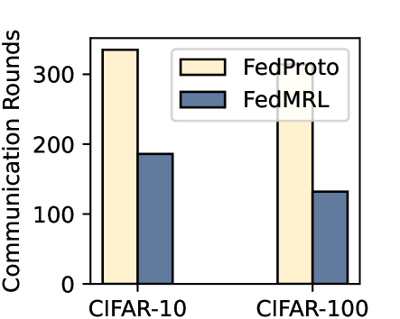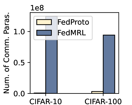</details> Figure 4: Communication rounds, number of communicated parameters, and computation FLOPs required to reach $90\%$ and $50\%$ average test accuracy targets on CIFAR-10 and CIFAR-100. 5.2.3 Communication Cost We record the communication rounds and the number of parameters sent per client to achieve $90\%$ and $50\%$ target test average accuracy on CIFAR-10 and CIFAR-100, respectively. Figure 4 (left) shows that FedMRL requires fewer rounds and achieves faster convergence than FedProto. Figure 4 (middle) shows that FedMRL incurs higher communication costs than FedProto as it transmits the full homogeneous small model, while FedProto only transmits each local seen-class average representation between the server and the client. Nevertheless, FedMRL with an optional smaller representation dimension ( $d_{1}$ ) of the homogeneous small model still achieves higher communication efficiency than same-category mutual learning-based MHeteroFL baselines (FML, FedKD, FedAPEN) with a larger representation dimension. 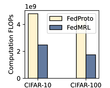5.2.4 Computation Overhead We also calculate the computation FLOPs consumed per client to reach $90\%$ and $50\%$ target average test accuracy on CIFAR-10 and CIFAR-100, respectively. Figure 4 (right) shows that FedMRL incurs lower computation costs than FedProto, owing to its faster convergence (i.e., fewer rounds) even with higher computation overhead per round due to the need to train an additional homogeneous small model and a linear representation projector. 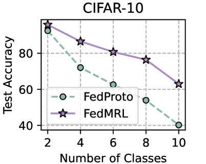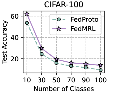5.3 Case Studies 5.3.1 Robustness to Non-IIDness (Class) We evaluate the robustness of FedMRL to different non-IIDnesses as a result of the number of classes assigned to each client under the ( $N=100,C=10\%$ ) setting. The fewer classes assigned to each client, the higher the non-IIDness. For CIFAR-10, we assign $\{2,4,...,10\}$ classes out of total $10$ classes to each client. For CIFAR-100, we assign $\{10,30,...,100\}$ classes out of total $100$ classes to each client. Figure 5 (left two) shows that FedMRL consistently achieves higher average test accuracy than the best-performing baseline - FedProto on both datasets, demonstrating its robustness to non-IIDness by class. <details> <summary>x15.png Details</summary>  ### Visual Description ## Line Chart: CIFAR-10 Test Accuracy vs. Number of Classes ### Overview The chart compares the test accuracy of two machine learning models, **FedProto** and **FedMRL**, across varying numbers of classes (2 to 10) on the CIFAR-10 dataset. Both models exhibit declining accuracy as the number of classes increases, with FedMRL consistently outperforming FedProto. ### Components/Axes - **X-axis**: "Number of Classes" (values: 2, 4, 6, 8, 10). - **Y-axis**: "Test Accuracy" (percentage, range: 40–100). - **Legend**: Located in the bottom-left corner, with: - **FedProto**: Dashed teal line with circular markers. - **FedMRL**: Solid purple line with star-shaped markers. ### Detailed Analysis 1. **FedProto (Teal Line)**: - Starts at ~90% accuracy for 2 classes. - Declines steadily to ~40% at 10 classes. - Data points: (2, 90), (4, 70), (6, 60), (8, 50), (10, 40). 2. **FedMRL (Purple Line)**: - Begins at ~95% accuracy for 2 classes. - Declines more gradually to ~60% at 10 classes. - Data points: (2, 95), (4, 85), (6, 80), (8, 75), (10, 60). ### Key Observations - **Downward Trend**: Both models show reduced accuracy as class complexity increases, reflecting the inherent difficulty of multi-class classification. - **Performance Gap**: FedMRL maintains a ~10–15% accuracy advantage over FedProto across all class counts. - **Steepest Drop**: FedProto’s accuracy drops sharply between 2 and 4 classes (~20% decrease), while FedMRL’s decline is more gradual. ### Interpretation The data suggests that **FedMRL** is more robust to class imbalance or complexity compared to **FedProto**, likely due to differences in their training methodologies (e.g., meta-learning vs. prototype-based learning). The consistent decline in accuracy for both models underscores the challenge of generalizing to larger class spaces in image classification tasks. Notably, FedProto’s steeper drop may indicate over-reliance on class-specific features that become less discriminative as class diversity increases. </details> <details> <summary>x16.png Details</summary>  ### Visual Description ## Line Graph: CIFAR-100 Test Accuracy vs. Number of Classes ### Overview The chart compares the test accuracy of two federated learning methods, **FedProto** and **FedMRL**, across varying numbers of classes (10 to 100) on the CIFAR-100 dataset. Both methods show declining accuracy as the number of classes increases, with FedMRL consistently outperforming FedProto. ### Components/Axes - **Title**: "CIFAR-100" (top-center). - **Y-Axis**: "Test Accuracy" (percentage, 0–60, linear scale). - **X-Axis**: "Number of Classes" (10–100, linear scale). - **Legend**: Top-right corner, with: - **FedProto**: Dashed green line with hollow circles. - **FedMRL**: Solid purple line with star markers. ### Detailed Analysis #### FedProto (Green Dashed Line) - **10 classes**: ~55% accuracy. - **30 classes**: ~25% accuracy. - **50 classes**: ~15% accuracy. - **70 classes**: ~12% accuracy. - **90 classes**: ~10% accuracy. - **100 classes**: ~8% accuracy. #### FedMRL (Purple Solid Line) - **10 classes**: ~60% accuracy. - **30 classes**: ~30% accuracy. - **50 classes**: ~20% accuracy. - **70 classes**: ~15% accuracy. - **90 classes**: ~13% accuracy. - **100 classes**: ~12% accuracy. ### Key Observations 1. **Declining Trends**: Both methods exhibit a monotonic decline in accuracy as the number of classes increases. 2. **Performance Gap**: FedMRL maintains a ~10–15% accuracy advantage over FedProto across all class counts. 3. **Convergence**: The gap narrows slightly at 100 classes (FedMRL: 12% vs. FedProto: 8%), but FedMRL remains superior. 4. **Steepest Drop**: FedProto’s accuracy drops sharply from 55% to 25% between 10 and 30 classes, while FedMRL’s decline is more gradual. ### Interpretation The data suggests that **FedMRL** is more robust to class imbalance or complexity in CIFAR-100 compared to **FedProto**. The steeper initial drop for FedProto implies it may rely heavily on class-specific features that become less discriminative as class diversity increases. FedMRL’s slower decline could indicate better generalization or more effective feature aggregation across classes. However, both methods struggle significantly beyond 50 classes, highlighting the challenge of scalability in federated learning for high-dimensional datasets like CIFAR-100. The convergence at 100 classes suggests that further improvements may require architectural innovations or hybrid approaches. </details> <details> <summary>x17.png Details</summary>  ### Visual Description ## Line Chart: CIFAR-10 Test Accuracy vs. α Parameter ### Overview The chart compares the test accuracy of two machine learning models (FedProto and FedMRL) across varying values of the hyperparameter α (alpha) on the CIFAR-10 dataset. Test accuracy is measured on the y-axis (40-60%), while α ranges from 0.1 to 0.5 on the x-axis. ### Components/Axes - **X-axis (α)**: Discrete values at 0.1, 0.2, 0.3, 0.4, 0.5 - **Y-axis (Test Accuracy)**: Percentage scale from 40% to 60% - **Legend**: Located in the top-right corner, with: - **FedProto**: Dashed teal line with circle markers - **FedMRL**: Solid purple line with star markers ### Detailed Analysis 1. **FedProto (Teal Line)**: - Starts at ~45% accuracy at α=0.1 - Gradually declines to ~40% by α=0.5 - Slight plateau between α=0.3 and α=0.5 (~40-41%) - Trend: Consistent downward slope with minimal fluctuation 2. **FedMRL (Purple Line)**: - Begins at ~65% accuracy at α=0.1 - Drops sharply to ~63% at α=0.3 - Stabilizes between α=0.3 and α=0.5 (~63-64%) - Trend: Initial decline followed by plateau ### Key Observations - FedMRL consistently outperforms FedProto across all α values (20-30% higher accuracy) - FedProto shows a steady degradation as α increases - FedMRL demonstrates robustness to α changes after initial drop - No overlapping confidence intervals between the two models ### Interpretation The data suggests FedMRL is significantly more robust to hyperparameter α variations than FedProto for CIFAR-10 classification. The stability of FedMRL's accuracy after α=0.3 indicates potential insensitivity to this parameter in later training stages. In contrast, FedProto's continuous decline implies α plays a critical role in its performance. These results could guide hyperparameter tuning strategies, with FedMRL being preferable for scenarios requiring α flexibility. The stark performance gap raises questions about FedProto's architectural limitations or training dynamics under varying α conditions. </details> <details> <summary>x18.png Details</summary>  ### Visual Description ## Line Chart: CIFAR-100 Test Accuracy vs. α ### Overview The chart compares the test accuracy of two machine learning methods (FedProto and FedMRL) across varying values of α (0.1 to 0.5) on the CIFAR-100 dataset. Test accuracy is measured on the y-axis (10–14), while α is plotted on the x-axis. Two distinct trends are observed: FedProto shows a steady decline, while FedMRL exhibits a sharp initial drop followed by stabilization. ### Components/Axes - **X-axis (α)**: Labeled "α" with values 0.1, 0.2, 0.3, 0.4, 0.5. - **Y-axis (Test Accuracy)**: Labeled "Test Accuracy" with values 10, 12, 14. - **Legend**: Located in the top-right corner, with: - **FedProto**: Dashed teal line with hollow circles. - **FedMRL**: Solid purple line with star markers. ### Detailed Analysis 1. **FedProto (Teal Line)**: - Starts at **~12.2** when α = 0.1. - Declines steadily to **~9.8** at α = 0.5. - Intermediate points: ~11.0 (α=0.2), ~10.0 (α=0.3), ~9.5 (α=0.4). 2. **FedMRL (Purple Line)**: - Begins at **~15.0** when α = 0.1. - Drops sharply to **~13.5** at α = 0.3. - Stabilizes with a slight increase to **~12.5** at α = 0.5. - Intermediate points: ~14.0 (α=0.2), ~13.5 (α=0.3), ~12.5 (α=0.5). ### Key Observations - FedMRL consistently outperforms FedProto across all α values. - FedProto’s decline is linear, while FedMRL’s performance plateaus after α = 0.3. - The largest gap between methods occurs at α = 0.1 (~2.8 accuracy difference). ### Interpretation The data suggests that FedMRL is more robust to changes in α, maintaining higher accuracy even as α increases. FedProto’s performance degrades linearly, indicating sensitivity to α. The stabilization of FedMRL at higher α values implies potential adaptability to model complexity or noise in the CIFAR-100 dataset. The sharp drop in FedMRL’s accuracy between α = 0.1 and 0.3 may reflect a threshold where model assumptions become less valid. These trends highlight the importance of tuning α for federated learning frameworks on non-IID datasets like CIFAR-100. 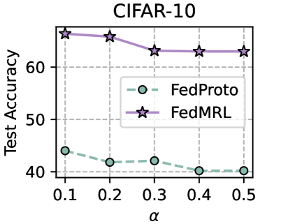</details> Figure 5: Robustness to non-IIDness (Class & Dirichlet). <details> <summary>x19.png Details</summary>  ### Visual Description ## Line Chart: CIFAR-10 Test Accuracy vs. d1 Parameter ### Overview The chart illustrates the relationship between the hyperparameter `d1` and test accuracy for the FedMRL algorithm on the CIFAR-10 dataset. Test accuracy is plotted on the y-axis (93–95 range), while `d1` values (200, 400) are on the x-axis. The data shows a non-linear trend with a pronounced dip and recovery. ### Components/Axes - **Title**: "CIFAR-10" (top-center) - **Y-Axis**: "Test Accuracy" (93–95, increments of 1) - **X-Axis**: "d1" (200, 400, increments of 200) - **Legend**: "FedMRL" (purple dashed line with star markers, top-right) - **Data Series**: Single line with star markers (purple, dashed) ### Detailed Analysis - **Data Points**: - At `d1 = 200`: Test accuracy ≈ 93.5 (lowest point, marked with a star) - At `d1 = 400`: Test accuracy ≈ 94.5 (recovery phase, marked with a star) - **Trend**: - The line starts at 95 (unlabeled `d1`), drops sharply to 93.5 at `d1 = 200`, then rises to 94.5 at `d1 = 400`. The pattern suggests a V-shaped curve with a trough at `d1 = 200`. ### Key Observations 1. **Performance Dip**: Test accuracy decreases significantly at `d1 = 200`, indicating suboptimal performance at this hyperparameter value. 2. **Recovery**: Accuracy improves at `d1 = 400`, suggesting a potential optimal range beyond `d1 = 200`. 3. **Non-Linearity**: The relationship between `d1` and accuracy is not monotonic, highlighting sensitivity to hyperparameter tuning. ### Interpretation The chart demonstrates that FedMRL's performance on CIFAR-10 is highly dependent on the `d1` hyperparameter. The sharp drop at `d1 = 200` implies that this value may represent a critical threshold where model stability or learning dynamics degrade. The subsequent recovery at `d1 = 400` suggests that larger values of `d1` could mitigate this issue, though further exploration beyond `d1 = 400` would be needed to confirm an optimal range. This sensitivity underscores the importance of hyperparameter optimization in federated learning frameworks for image classification tasks. 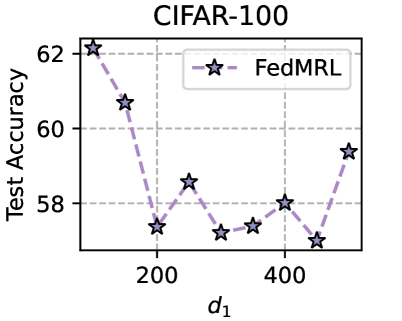</details> <details> <summary>x20.png Details</summary>  ### Visual Description ## Line Chart: CIFAR-100 Test Accuracy vs. d₁ ### Overview The chart illustrates the relationship between a parameter `d₁` and test accuracy for the FedMRL algorithm on the CIFAR-100 dataset. Test accuracy is plotted on the y-axis (58–62), while `d₁` values (200, 400, 600) are on the x-axis. The data is represented by a dashed purple line with star markers. ### Components/Axes - **Title**: "CIFAR-100" (top-center). - **X-axis**: Labeled `d₁`, with tick marks at 200, 400, and 600. - **Y-axis**: Labeled "Test Accuracy", scaled from 58 to 62. - **Legend**: Located in the top-right corner, labeled "FedMRL" with a purple dashed line and star markers. - **Data Series**: A single line (purple dashed) with star markers (black outline, purple fill). ### Detailed Analysis - **Data Points**: - At `d₁ = 200`: Test accuracy ≈ 62 (peak). - At `d₁ = 400`: Test accuracy ≈ 58 (trough). - At `d₁ = 600`: Test accuracy ≈ 59 (partial recovery). - **Trend**: The line starts at a high accuracy (62) at `d₁ = 200`, sharply declines to 58 at `d₁ = 400`, then slightly increases to 59 at `d₁ = 600`. ### Key Observations 1. **Initial Peak**: The highest accuracy (62) occurs at the smallest `d₁` value (200). 2. **Significant Dip**: A sharp drop to 58 at `d₁ = 400` suggests sensitivity to parameter increases. 3. **Partial Recovery**: A modest rise to 59 at `d₁ = 600` indicates potential non-linear behavior. ### Interpretation The data suggests that FedMRL's performance on CIFAR-100 is highly dependent on `d₁`. The initial peak at `d₁ = 200` may reflect optimal parameter settings, while the subsequent drop at `d₁ = 400` highlights a critical threshold where performance degrades. The partial recovery at `d₁ = 600` could imply a secondary optimal region or a stabilizing effect at higher values. This non-linear trend underscores the importance of fine-tuning `d₁` for FedMRL in CIFAR-100 applications. The anomaly at `d₁ = 600` warrants further investigation to determine if it represents a local maximum or a transitional phase. 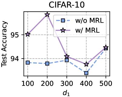</details> <details> <summary>x21.png Details</summary>  ### Visual Description ## Line Graph: CIFAR-10 Test Accuracy vs. d1 Parameter ### Overview The chart compares test accuracy (y-axis) against a parameter `d1` (x-axis) for two configurations: "w/o MRL" (without MRL) and "w/ MRL" (with MRL). The data is plotted using dashed blue lines with square markers for "w/o MRL" and solid purple lines with star markers for "w/ MRL". The graph highlights performance trends across five `d1` values (100, 200, 300, 400, 500). ### Components/Axes - **X-axis (d1)**: Labeled "d₁", with discrete values at 100, 200, 300, 400, 500. - **Y-axis (Test Accuracy)**: Labeled "Test Accuracy", ranging from 94 to 95.5. - **Legend**: Located in the top-right corner, with two entries: - **Blue dashed line + squares**: "w/o MRL" - **Purple solid line + stars**: "w/ MRL" ### Detailed Analysis #### "w/o MRL" (Blue Dashed Line) - **Trend**: Relatively flat with minor fluctuations. - **Data Points**: - d1=100: ~94.0 - d1=200: ~94.0 - d1=300: ~94.1 - d1=400: ~93.7 - d1=500: ~94.5 #### "w/ MRL" (Purple Solid Line) - **Trend**: Peaks at d1=200, then declines and recovers. - **Data Points**: - d1=100: ~95.0 - d1=200: ~95.5 (peak) - d1=300: ~94.1 - d1=400: ~93.8 - d1=500: ~94.5 ### Key Observations 1. **Performance Gap**: "w/ MRL" consistently outperforms "w/o MRL" except at d1=500, where accuracies converge (~94.5). 2. **Peak at d1=200**: "w/ MRL" achieves its highest accuracy (95.5) at d1=200, suggesting optimal performance at this parameter value. 3. **Dip at d1=400**: Both configurations show a notable drop in accuracy at d1=400, with "w/ MRL" falling to ~93.8. 4. **Stability**: "w/o MRL" exhibits smoother trends, while "w/ MRL" shows sharper fluctuations. ### Interpretation The graph demonstrates that MRL improves test accuracy for most `d1` values, particularly at lower ranges (d1=100–300). However, the performance advantage diminishes at higher `d1` values (e.g., d1=500). The dip at d1=400 for "w/ MRL" may indicate a sensitivity to parameter tuning or overfitting risks. The convergence at d1=500 suggests diminishing returns for MRL as `d1` increases. This could imply that MRL’s benefits are context-dependent, requiring careful calibration of `d1` for optimal results. ### Spatial Grounding & Validation - Legend placement (top-right) aligns with standard chart conventions. - Line colors and markers match legend labels: - Blue dashed line + squares = "w/o MRL" (confirmed at all points). - Purple solid line + stars = "w/ MRL" (confirmed at all points). - Axis labels and scales are explicitly defined, with no ambiguity in units or ranges. ### Uncertainties - Exact numerical values are approximate (e.g., 94.5 ±0.1) due to visual estimation from the graph. - The cause of the d1=400 dip remains unexplained by the chart alone. 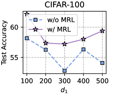</details> <details> <summary>x22.png Details</summary>  ### Visual Description ## Line Chart: CIFAR-100 Test Accuracy vs. d1 Parameter ### Overview The chart compares test accuracy performance of two configurations ("w/o MRL" and "w/ MRL") across varying values of the parameter *d1* (100 to 500). Two data series are plotted: a dashed blue line with square markers ("w/o MRL") and a solid purple line with star markers ("w/ MRL"). The y-axis represents test accuracy (55-60 range), while the x-axis shows *d1* values in increments of 100. ### Components/Axes - **Title**: "CIFAR-100" (top center) - **Y-axis**: "Test Accuracy" (55-60, linear scale) - **X-axis**: "d1" (100-500, linear scale) - **Legend**: Top-right corner, with: - Blue dashed line + square markers: "w/o MRL" - Purple solid line + star markers: "w/ MRL" ### Detailed Analysis 1. **w/o MRL (Blue Squares)**: - d1=100: ~58.5 accuracy - d1=200: ~56.0 accuracy - d1=300: ~53.0 accuracy (notable dip) - d1=400: ~56.0 accuracy (partial recovery) - d1=500: ~54.5 accuracy (final decline) 2. **w/ MRL (Purple Stars)**: - d1=100: ~61.0 accuracy - d1=200: ~57.0 accuracy - d1=300: ~57.0 accuracy (stable) - d1=400: ~58.0 accuracy (improvement) - d1=500: ~59.5 accuracy (peak performance) ### Key Observations - **Consistent Advantage**: "w/ MRL" maintains ~2-3% higher accuracy across all *d1* values compared to "w/o MRL". - **Volatility**: "w/o MRL" shows significant fluctuations, particularly a sharp drop at d1=300. - **Scaling Behavior**: Both configurations show improved performance at higher *d1* values, with "w/ MRL" demonstrating stronger scaling. ### Interpretation The data suggests that the MRL (likely a machine learning regularization technique) provides robust performance improvements across different *d1* parameter settings. The "w/ MRL" configuration shows more stable and scalable behavior, particularly at larger *d1* values (400-500), where it achieves near-peak accuracy. The "w/o MRL" configuration exhibits sensitivity to *d1* changes, with a critical performance drop at d1=300 that doesn't fully recover at higher values. This pattern implies MRL may help mitigate parameter sensitivity in CIFAR-100 classification tasks, making it valuable for optimizing model generalization in resource-constrained scenarios. </details> Figure 6: Left two: sensitivity analysis results. Right two: ablation study results. 5.3.2 Robustness to Non-IIDness (Dirichlet) We also test the robustness of FedMRL to various non-IIDnesses controlled by $\alpha$ in the Dirichlet function under the ( $N=100,C=10\%$ ) setting. A smaller $\alpha$ indicates a higher non-IIDness. For both datasets, we vary $\alpha$ in the range of $\{0.1,...,0.5\}$ . Figure 5 (right two) shows that FedMRL significantly outperforms FedProto under all non-IIDness settings, validating its robustness to Dirichlet non-IIDness. 5.3.3 Sensitivity Analysis - $d_{1}$ FedMRL relies on a hyperparameter $d_{1}$ - the representation dimension of the homogeneous small model. To evaluate its sensitivity to $d_{1}$ , we test FedMRL with $d_{1}=\{100,150,...,500\}$ under the ( $N=100,C=10\%$ ) setting. Figure 6 (left two) shows that smaller $d_{1}$ values result in higher average test accuracy on both datasets. It is clear that a smaller $d_{1}$ also reduces communication and computation overheads, thereby helping FedMRL achieve the best trade-off among model performance, communication efficiency, and computational efficiency. 5.4 Ablation Study We conduct ablation experiments to validate the usefulness of MRL. For FedMRL with MRL, the global header and the local header learn multi-granularity representations. For FedMRL without MRL, we directly input the representation fused by the representation projector into the client’s local header for loss computation (i.e., we do not extract Matryoshka Representations and remove the global header). Figure 6 (right two) shows that FedMRL with MRL consistently outperforms FedMRL without MRL, demonstrating the effectiveness of the design to incorporate MRL into MHeteroFL. Besides, the accuracy gap between them decreases as $d_{1}$ rises. This shows that as the global and local headers learn increasingly overlapping representation information, the benefits of MRL are reduced. 6 Conclusions This paper proposes a novel MHeteroFL approach - FedMRL - to jointly address data, system and model heterogeneity challenges in FL. The key design insight is the addition of a global homogeneous small model shared by FL clients for enhanced knowledge interaction among heterogeneous local models. Adaptive personalized representation fusion and multi-granularity Matryoshka Representations learning further boosts model learning capability. The client and the server only need to exchange the homogeneous small model, while the clients’ heterogeneous local models and data remain unexposed, thereby enhancing the preservation of both model and data privacy. Theoretical analysis shows that FedMRL is guaranteed to converge over time. Extensive experiments demonstrate that FedMRL significantly outperforms state-of-the-art models regarding test accuracy, while incurring low communication and computation costs. Appendix D discusses FedMRL ’s privacy, communication and computation. Appendix E elaborates FedMRL ’s border impact and limitations. References - [1] Jin-Hyun Ahn et al. Wireless federated distillation for distributed edge learning with heterogeneous data. In Proc. PIMRC, pages 1–6, Istanbul, Turkey, 2019. IEEE. - [2] Jin-Hyun Ahn et al. Cooperative learning VIA federated distillation OVER fading channels. In Proc. ICASSP, pages 8856–8860, Barcelona, Spain, 2020. IEEE. - [3] Samiul Alam et al. Fedrolex: Model-heterogeneous federated learning with rolling sub-model extraction. In Proc. NeurIPS, virtual, 2022. . - [4] Sara Babakniya et al. Revisiting sparsity hunting in federated learning: Why does sparsity consensus matter? Transactions on Machine Learning Research, 1(1):1, 2023. - [5] Yun-Hin Chan, Rui Zhou, Running Zhao, Zhihan JIANG, and Edith C. H. Ngai. Internal cross-layer gradients for extending homogeneity to heterogeneity in federated learning. In Proc. ICLR, page 1, Vienna, Austria, 2024. OpenReview.net. - [6] Hongyan Chang et al. Cronus: Robust and heterogeneous collaborative learning with black-box knowledge transfer. In Proc. NeurIPS Workshop, virtual, 2021. . - [7] Jiangui Chen et al. Fedmatch: Federated learning over heterogeneous question answering data. In Proc. CIKM, pages 181–190, virtual, 2021. ACM. - [8] Sijie Cheng et al. Fedgems: Federated learning of larger server models via selective knowledge fusion. CoRR, abs/2110.11027, 2021. - [9] Yae Jee Cho et al. Heterogeneous ensemble knowledge transfer for training large models in federated learning. In Proc. IJCAI, pages 2881–2887, virtual, 2022. ijcai.org. - [10] Liam Collins et al. Exploiting shared representations for personalized federated learning. In Proc. ICML, volume 139, pages 2089–2099, virtual, 2021. PMLR. - [11] Enmao Diao. Heterofl: Computation and communication efficient federated learning for heterogeneous clients. In Proc. ICLR, page 1, Virtual Event, Austria, 2021. OpenReview.net. - [12] Xuan Gong et al. Federated learning via input-output collaborative distillation. In Proc. AAAI, pages 22058–22066, Vancouver, Canada, 2024. AAAI Press. - [13] Chaoyang He et al. Group knowledge transfer: Federated learning of large cnns at the edge. In Proc. NeurIPS, virtual, 2020. . - [14] S. Horváth. FjORD: Fair and accurate federated learning under heterogeneous targets with ordered dropout. In Proc. NIPS, pages 12876–12889, Virtual, 2021. OpenReview.net. - [15] Wenke Huang et al. Few-shot model agnostic federated learning. In Proc. MM, pages 7309–7316, Lisboa, Portugal, 2022. ACM. - [16] Wenke Huang et al. Learn from others and be yourself in heterogeneous federated learning. In Proc. CVPR, pages 10133–10143, virtual, 2022. IEEE. - [17] Sohei Itahara et al. Distillation-based semi-supervised federated learning for communication-efficient collaborative training with non-iid private data. IEEE Trans. Mob. Comput., 22(1):191–205, 2023. - [18] Jaehee Jang et al. Fedclassavg: Local representation learning for personalized federated learning on heterogeneous neural networks. In Proc. ICPP, pages 76:1–76:10, virtual, 2022. ACM. - [19] Eunjeong Jeong et al. Communication-efficient on-device machine learning: Federated distillation and augmentation under non-iid private data. In Proc. NeurIPS Workshop on Machine Learning on the Phone and other Consumer Devices, virtual, 2018. . - [20] Alex Krizhevsky et al. Learning multiple layers of features from tiny images. Toronto, ON, Canada, , 2009. - [21] Aditya Kusupati et al. Matryoshka representation learning. In Proc. NeurIPS, New Orleans, LA, USA, 2022. - [22] Daliang Li and Junpu Wang. Fedmd: Heterogenous federated learning via model distillation. In Proc. NeurIPS Workshop, virtual, 2019. . - [23] Qinbin Li et al. Practical one-shot federated learning for cross-silo setting. In Proc. IJCAI, pages 1484–1490, virtual, 2021. ijcai.org. - [24] Paul Pu Liang et al. Think locally, act globally: Federated learning with local and global representations. arXiv preprint arXiv:2001.01523, 1(1), 2020. - [25] Tao Lin et al. Ensemble distillation for robust model fusion in federated learning. In Proc. NeurIPS, virtual, 2020. . - [26] Chang Liu et al. Completely heterogeneous federated learning. CoRR, abs/2210.15865, 2022. - [27] Disha Makhija et al. Architecture agnostic federated learning for neural networks. In Proc. ICML, volume 162, pages 14860–14870, virtual, 2022. PMLR. - [28] Koji Matsuda et al. Fedme: Federated learning via model exchange. In Proc. SDM, pages 459–467, Alexandria, VA, USA, 2022. SIAM. - [29] Brendan McMahan et al. Communication-efficient learning of deep networks from decentralized data. In Proc. AISTATS, volume 54, pages 1273–1282, Fort Lauderdale, FL, USA, 2017. PMLR. - [30] Duy Phuong Nguyen et al. Enhancing heterogeneous federated learning with knowledge extraction and multi-model fusion. In Proc. SC Workshop, pages 36–43, Denver, CO, USA, 2023. ACM. - [31] Jaehoon Oh et al. Fedbabu: Toward enhanced representation for federated image classification. In Proc. ICLR, virtual, 2022. OpenReview.net. - [32] Sejun Park et al. Towards understanding ensemble distillation in federated learning. In Proc. ICML, volume 202, pages 27132–27187, Honolulu, Hawaii, USA, 2023. PMLR. - [33] Krishna Pillutla et al. Federated learning with partial model personalization. In Proc. ICML, volume 162, pages 17716–17758, virtual, 2022. PMLR. - [34] Zhen Qin et al. Fedapen: Personalized cross-silo federated learning with adaptability to statistical heterogeneity. In Proc. KDD, pages 1954–1964, Long Beach, CA, USA, 2023. ACM. - [35] Felix Sattler et al. Fedaux: Leveraging unlabeled auxiliary data in federated learning. IEEE Trans. Neural Networks Learn. Syst., 1(1):1–13, 2021. - [36] Felix Sattler et al. CFD: communication-efficient federated distillation via soft-label quantization and delta coding. IEEE Trans. Netw. Sci. Eng., 9(4):2025–2038, 2022. - [37] Aviv Shamsian et al. Personalized federated learning using hypernetworks. In Proc. ICML, volume 139, pages 9489–9502, virtual, 2021. PMLR. - [38] Tao Shen et al. Federated mutual learning. CoRR, abs/2006.16765, 2020. - [39] Xiaorong Shi, Liping Yi, Xiaoguang Liu, and Gang Wang. FFEDCL: fair federated learning with contrastive learning. In Proc. ICASSP, Rhodes Island, Greece,, pages 1–5. IEEE, 2023. - [40] Alysa Ziying Tan et al. Towards personalized federated learning. IEEE Trans. Neural Networks Learn. Syst., 1(1):1–17, 2022. - [41] Yue Tan et al. Fedproto: Federated prototype learning across heterogeneous clients. In Proc. AAAI, pages 8432–8440, virtual, 2022. AAAI Press. - [42] Jiaqi Wang et al. Towards personalized federated learning via heterogeneous model reassembly. In Proc. NeurIPS, page 13, New Orleans, Louisiana, USA, 2023. OpenReview.net. - [43] Chuhan Wu et al. Communication-efficient federated learning via knowledge distillation. Nature Communications, 13(1):2032, 2022. - [44] Liping Yi, Xiaorong Shi, Nan Wang, Gang Wang, Xiaoguang Liu, Zhuan Shi, and Han Yu. pfedkt: Personalized federated learning with dual knowledge transfer. Knowledge-Based Systems, 292:111633, 2024. - [45] Liping Yi, Xiaorong Shi, Nan Wang, Ziyue Xu, Gang Wang, and Xiaoguang Liu. pfedlhns: Personalized federated learning via local hypernetworks. In Proc. ICANN, volume 1, page 516–528. Springer, 2023. - [46] Liping Yi, Xiaorong Shi, Nan Wang, Jinsong Zhang, Gang Wang, and Xiaoguang Liu. Fedpe: Adaptive model pruning-expanding for federated learning on mobile devices. IEEE Transactions on Mobile Computing, pages 1–18, 2024. - [47] Liping Yi, Xiaorong Shi, Wenrui Wang, Gang Wang, and Xiaoguang Liu. Fedrra: Reputation-aware robust federated learning against poisoning attacks. In Proc. IJCNN, pages 1–8. IEEE, 2023. - [48] Liping Yi, Gang Wang, and Xiaoguang Liu. QSFL: A two-level uplink communication optimization framework for federated learning. In Proc. ICML, volume 162, pages 25501–25513. PMLR, 2022. - [49] Liping Yi, Gang Wang, Xiaoguang Liu, Zhuan Shi, and Han Yu. Fedgh: Heterogeneous federated learning with generalized global header. In Proceedings of the 31st ACM International Conference on Multimedia (ACM MM’23), page 11, Canada, 2023. ACM. - [50] Liping Yi, Han Yu, Chao Ren, Heng Zhang, Gang Wang, Xiaoguang Liu, and Xiaoxiao Li. pfedafm: Adaptive feature mixture for batch-level personalization in heterogeneous federated learning. CoRR, abs/2404.17847, 2024. - [51] Liping Yi, Han Yu, Chao Ren, Heng Zhang, Gang Wang, Xiaoguang Liu, and Xiaoxiao Li. pfedmoe: Data-level personalization with mixture of experts for model-heterogeneous personalized federated learning. CoRR, abs/2402.01350, 2024. - [52] Liping Yi, Han Yu, Zhuan Shi, Gang Wang, Xiaoguang Liu, Lizhen Cui, and Xiaoxiao Li. FedSSA: Semantic Similarity-based Aggregation for Efficient Model-Heterogeneous Personalized Federated Learning. In IJCAI, 2024. - [53] Liping Yi, Han Yu, Gang Wang, and Xiaoguang Liu. Fedlora: Model-heterogeneous personalized federated learning with lora tuning. CoRR, abs/2310.13283, 2023. - [54] Liping Yi, Han Yu, Gang Wang, and Xiaoguang Liu. pfedes: Model heterogeneous personalized federated learning with feature extractor sharing. CoRR, abs/2311.06879, 2023. - [55] Liping Yi, Jinsong Zhang, Rui Zhang, Jiaqi Shi, Gang Wang, and Xiaoguang Liu. Su-net: An efficient encoder-decoder model of federated learning for brain tumor segmentation. In Proc. ICANN, volume 12396, pages 761–773. Springer, 2020. - [56] Fuxun Yu et al. Fed2: Feature-aligned federated learning. In Proc. KDD, pages 2066–2074, virtual, 2021. ACM. - [57] Sixing Yu et al. Resource-aware federated learning using knowledge extraction and multi-model fusion. CoRR, abs/2208.07978, 2022. - [58] Jianqing Zhang, Yang Liu, Yang Hua, and Jian Cao. Fedtgp: Trainable global prototypes with adaptive-margin-enhanced contrastive learning for data and model heterogeneity in federated learning. In Proc. AAAI, pages 16768–16776, Vancouver, Canada, 2024. AAAI Press. - [59] Jie Zhang et al. Parameterized knowledge transfer for personalized federated learning. In Proc. NeurIPS, pages 10092–10104, virtual, 2021. OpenReview.net. - [60] Jie Zhang et al. Towards data-independent knowledge transfer in model-heterogeneous federated learning. IEEE Trans. Computers, 72(10):2888–2901, 2023. - [61] Lan Zhang et al. Fedzkt: Zero-shot knowledge transfer towards resource-constrained federated learning with heterogeneous on-device models. In Proc. ICDCS, pages 928–938, virtual, 2022. IEEE. - [62] Zhilu Zhang and Mert R. Sabuncu. Generalized cross entropy loss for training deep neural networks with noisy labels. In Proc. NeurIPS, pages 8792–8802, Montréal, Canada, 2018. Curran Associates Inc. - [63] Zhuangdi Zhu et al. Data-free knowledge distillation for heterogeneous federated learning. In Proc. ICML, volume 139, pages 12878–12889, virtual, 2021. PMLR. - [64] Zhuangdi Zhu et al. Resilient and communication efficient learning for heterogeneous federated systems. In Proc. ICML, volume 162, pages 27504–27526, virtual, 2022. PMLR. Appendix A Pseudo codes of FedMRL Input: $N$ , total number of clients; $K$ , number of selected clients in one round; $T$ , total number of rounds; $\eta_{\omega}$ , learning rate of client local heterogeneous models; $\eta_{\theta}$ , learning rate of homogeneous small model; $\eta_{\varphi}$ , learning rate of the representation projector. Output: client whole models removing the global header $[\mathcal{G}(\theta^{ex,T-1})\circ\mathcal{F}_{0}(\omega_{0}^{T-1})|\mathcal{P% }_{0}(\varphi_{0}^{T-1}),...,\mathcal{G}(\theta^{ex,T-1})\circ\mathcal{F}_{% N-1}(\omega_{N-1}^{T-1})|\mathcal{P}_{N-1}(\varphi_{N-1}^{T-1})]$ . Randomly initialize the global homogeneous small model $\mathcal{G}(\theta^{\mathbf{0}})$ , client local heterogeneous models $[\mathcal{F}_{0}(\omega_{0}^{0}),...,\mathcal{F}_{N-1}(\omega_{N-1}^{0})]$ and local heterogeneous representation projectors $[\mathcal{P}_{0}(\varphi_{0}^{0}),...,\mathcal{P}_{N-1}(\varphi_{N-1}^{0})]$ . for each round t=1,…,T-1 do // Server Side: $S^{t}$ $←$ Randomly sample $K$ clients from $N$ clients; Broadcast the global homogeneous small model $\theta^{t-1}$ to sampled $K$ clients; $\theta_{k}^{t}←$ ClientUpdate ( $\theta^{t-1}$ ); /* Aggregate Local Homogeneous Small Models */ $\theta^{t}=\sum_{k=0}^{K-1}{\frac{n_{k}}{n}\theta_{k}^{t}}$ . // ClientUpdate: Receive the global homogeneous small model $\theta^{t-1}$ from the server; for $k∈ S^{t}$ do /* Local Training with MRL */ for $(\boldsymbol{x}_{i},y_{i})∈ D_{k}$ do $\boldsymbol{\mathcal{R}}_{i}^{\mathcal{G}}=\ \mathcal{G}^{ex}({\boldsymbol{x}_% {i};\theta}^{ex,t-1}),\boldsymbol{\mathcal{R}}_{i}^{\mathcal{F}_{k}}=\ % \mathcal{F}_{k}^{ex}(\boldsymbol{x}_{i};\omega_{k}^{ex,t-1})$ ; $\boldsymbol{\mathcal{R}}_{i}=\boldsymbol{\mathcal{R}}_{i}^{\mathcal{G}}\circ% \boldsymbol{\mathcal{R}}_{i}^{\mathcal{F}_{k}}$ ; ${\widetilde{\boldsymbol{\mathcal{R}}}}_{i}=\mathcal{P}_{k}(\boldsymbol{% \mathcal{R}}_{i}{;\varphi}_{k}^{t-1})$ ; ${\widetilde{\boldsymbol{\mathcal{R}}}}_{i}^{lc}={{\widetilde{\boldsymbol{% \mathcal{R}}}}_{i}}^{1:d_{1}},{\widetilde{\boldsymbol{\mathcal{R}}}}_{i}^{hf}=% {{\widetilde{\boldsymbol{\mathcal{R}}}}_{i}}^{1:d_{2}}$ ; ${\hat{{y}}}_{i}^{\mathcal{G}}=\mathcal{G}^{hd}({\widetilde{\boldsymbol{% \mathcal{R}}}}_{i}^{lc};\theta^{hd,t-1});{\hat{{y}}}_{i}^{\mathcal{F}_{k}}=% \mathcal{F}_{k}^{hd}(\omega_{k}^{hd,t-1})$ ; $\ell_{i}^{\mathcal{G}}=\ell({\hat{{y}}}_{i}^{\mathcal{G}},y_{i});\ell_{i}^{% \mathcal{F}_{k}}=\ell({\hat{{y}}}_{i}^{\mathcal{F}_{k}},y_{i})$ ; $\ell_{i}=m_{i}^{\mathcal{G}}·\ell_{i}^{\mathcal{G}}+m_{i}^{\mathcal{F}_{k}% }·\ell_{i}^{\mathcal{F}_{k}}$ ; $\theta_{k}^{t}←\theta^{t-1}-\eta_{\theta}∇\ell_{i}$ ; $\omega_{k}^{t}←\omega_{k}^{t-1}-\eta_{\omega}∇\ell_{i}$ ; $\varphi_{k}^{t}←\varphi_{k}^{t-1}-\eta_{\varphi}∇\ell_{i}$ ; end for Upload updated local homogeneous small model $\theta_{k}^{t}$ to the server. end for end for Algorithm 1 FedMRL Appendix B Theoretical Proofs We first define the following additional notations. $t∈\{0,...,T-1\}$ denotes the $t$ -th round. $e∈\{0,1,...,E\}$ denotes the $e$ -th iteration of local training. $tE+0$ indicates that clients receive the global homogeneous small model $\mathcal{G}(\theta^{t})$ from the server before the $(t+1)$ -th round’s local training. $tE+e$ denotes the $e$ -th iteration of the $(t+1)$ -th round’s local training. $tE+E$ marks the ending of the $(t+1)$ -th round’s local training. After that, clients upload their updated local homogeneous small models to the server for aggregation. $\mathcal{W}_{k}(w_{k})$ denotes the whole model trained on client $k$ , including the global homogeneous small model $\mathcal{G}(\theta)$ , the client $k$ ’s local heterogeneous model $\mathcal{F}_{k}(\omega_{k})$ , and the personalized representation projector $\mathcal{P}_{k}(\varphi_{k})$ . $\eta$ is the learning rate of the whole model trained on client $k$ , including $\{\eta_{\theta},\eta_{\omega},\eta_{\boldsymbol{\varphi}}\}$ . **Assumption 1** *Lipschitz Smoothness. The gradients of client $k$ ’s whole local model $w_{k}$ are $L1$ –Lipschitz smooth [41], $$ \begin{gathered}\|\nabla\mathcal{L}_{k}^{t_{1}}(w_{k}^{t_{1}};\boldsymbol{x},y% )-\nabla\mathcal{L}_{k}^{t_{2}}(w_{k}^{t_{2}};\boldsymbol{x},y)\|\leq L_{1}\|w% _{k}^{t_{1}}-w_{k}^{t_{2}}\|,\\ \forall t_{1},t_{2}>0,k\in\{0,1,\ldots,N-1\},(\boldsymbol{x},y)\in D_{k}.\end{gathered} \tag{15} $$ The above formulation can be re-expressed as: $$ \mathcal{L}_{k}^{t_{1}}-\mathcal{L}_{k}^{t_{2}}\leq\langle\nabla\mathcal{L}_{k% }^{t_{2}},(w_{k}^{t_{1}}-w_{k}^{t_{2}})\rangle+\frac{L_{1}}{2}\|w_{k}^{t_{1}}-% w_{k}^{t_{2}}\|_{2}^{2}. \tag{16} $$* **Assumption 2** *Unbiased Gradient and Bounded Variance. Client $k$ ’s random gradient $g_{w,k}^{t}=∇\mathcal{L}_{k}^{t}(w_{k}^{t};\mathcal{B}_{k}^{t})$ ( $\mathcal{B}$ is a batch of local data) is unbiased, $$ \mathbb{E}_{\mathcal{B}_{k}^{t}\subseteq D_{k}}[g_{w,k}^{t}]=\nabla\mathcal{L}% _{k}^{t}(w_{k}^{t}), \tag{17} $$ and the variance of random gradient $g_{w,k}^{t}$ is bounded by: $$ \begin{split}\mathbb{E}_{\mathcal{B}_{k}^{t}\subseteq D_{k}}[\|\nabla\mathcal{% L}_{k}^{t}(w_{k}^{t};\mathcal{B}_{k}^{t})-\nabla\mathcal{L}_{k}^{t}(w_{k}^{t})% \|_{2}^{2}]\leq\sigma^{2}.\end{split} \tag{18} $$* **Assumption 3** *Bounded Parameter Variation. The parameter variations of the homogeneous small model $\theta_{k}^{t}$ and $\theta^{t}$ before and after aggregation at the FL server are bounded by: $$ {\|\theta^{t}-\theta_{k}^{t}\|}_{2}^{2}\leq\delta^{2}. \tag{19} $$* B.1 Proof of Lemma 1 **Proof 1** *An arbitrary client $k$ ’s local whole model $w$ can be updated by $w_{t+1}=w_{t}-\eta g_{w,t}$ in the (t+1)-th round, and following Assumption 1, we can obtain $$ \displaystyle\mathcal{L}_{tE+1} \displaystyle\leq\mathcal{L}_{tE+0}+\langle\nabla\mathcal{L}_{tE+0},(w_{tE+1}-% w_{tE+0})\rangle+\frac{L_{1}}{2}\|w_{tE+1}-w_{tE+0}\|_{2}^{2} \displaystyle=\mathcal{L}_{tE+0}-\eta\langle\nabla\mathcal{L}_{tE+0},g_{w,tE+0% }\rangle+\frac{L_{1}\eta^{2}}{2}\|g_{w,tE+0}\|_{2}^{2}. \tag{20} $$ Taking the expectation of both sides of the inequality concerning the random variable $\xi_{tE+0}$ , $$ \displaystyle\mathbb{E}[\mathcal{L}_{tE+1}] \displaystyle\leq\mathcal{L}_{tE+0}-\eta\mathbb{E}[\langle\nabla\mathcal{L}_{% tE+0},g_{w,tE+0}\rangle]+\frac{L_{1}\eta^{2}}{2}\mathbb{E}[\|g_{w,tE+0}\|_{2}^% {2}] \displaystyle\stackrel{{\scriptstyle(a)}}{{=}}\mathcal{L}_{tE+0}-\eta\|\nabla% \mathcal{L}_{tE+0}\|_{2}^{2}+\frac{L_{1}\eta^{2}}{2}\mathbb{E}[\|g_{w,tE+0}\|_% {2}^{2}] \displaystyle\stackrel{{\scriptstyle(b)}}{{\leq}}\mathcal{L}_{tE+0}-\eta\|% \nabla\mathcal{L}_{tE+0}\|_{2}^{2}+\frac{L_{1}\eta^{2}}{2}(\mathbb{E}[\|g_{w,% tE+0}\|]_{2}^{2}+\operatorname{Var}(g_{w,tE+0})) \displaystyle\stackrel{{\scriptstyle(c)}}{{=}}\mathcal{L}_{tE+0}-\eta\|\nabla% \mathcal{L}_{tE+0}\|_{2}^{2}+\frac{L_{1}\eta^{2}}{2}(\|\nabla\mathcal{L}_{tE+0% }\|_{2}^{2}+\operatorname{Var}(g_{w,tE+0})) \displaystyle\stackrel{{\scriptstyle(d)}}{{\leq}}\mathcal{L}_{tE+0}-\eta\|% \nabla\mathcal{L}_{tE+0}\|_{2}^{2}+\frac{L_{1}\eta^{2}}{2}(\|\nabla\mathcal{L}% _{tE+0}\|_{2}^{2}+\sigma^{2}) \displaystyle=\mathcal{L}_{tE+0}+(\frac{L_{1}\eta^{2}}{2}-\eta)\|\nabla% \mathcal{L}_{tE+0}\|_{2}^{2}+\frac{L_{1}\eta^{2}\sigma^{2}}{2}. \tag{21} $$ (a), (c), (d) follow Assumption 2 and (b) follows $Var(x)=\mathbb{E}[x^{2}]-(\mathbb{E}[x])^{2}$ . Taking the expectation of both sides of the inequality for the model $w$ over $E$ iterations, we obtain $$ \mathbb{E}[\mathcal{L}_{tE+1}]\leq\mathcal{L}_{tE+0}+(\frac{L_{1}\eta^{2}}{2}-% \eta)\sum_{e=1}^{E}\|\nabla\mathcal{L}_{tE+e}\|_{2}^{2}+\frac{L_{1}E\eta^{2}% \sigma^{2}}{2}. \tag{22} $$* B.2 Proof of Lemma 2 **Proof 2** *$$ \displaystyle\mathcal{L}_{(t+1)E+0} \displaystyle=\mathcal{L}_{(t+1)E}+\mathcal{L}_{(t+1)E+0}-\mathcal{L}_{(t+1)E} \displaystyle\stackrel{{\scriptstyle(a)}}{{\approx}}\mathcal{L}_{(t+1)E}+\eta% \|\theta_{(t+1)E+0}-\theta_{(t+1)E}\|_{2}^{2} \displaystyle\stackrel{{\scriptstyle(b)}}{{\leq}}\mathcal{L}_{(t+1)E}+\eta% \delta^{2}. \tag{23} $$ (a): we can use the gradient of parameter variations to approximate the loss variations, i.e., $\Delta\mathcal{L}≈\eta·\|\Delta\theta\|_{2}^{2}$ . (b) follows Assumption 3. Taking the expectation of both sides of the inequality to the random variable $\xi$ , we obtain $$ \mathbb{E}[\mathcal{L}_{(t+1)E+0}]\leq\mathbb{E}[\mathcal{L}_{tE+1}]+{\eta% \delta}^{2}. \tag{24} $$* B.3 Proof of Theorem 1 **Proof 3** *Substituting Lemma 1 into the right side of Lemma 2 ’s inequality, we obtain $$ \mathbb{E}[\mathcal{L}_{(t+1)E+0}]\leq\mathcal{L}_{tE+0}+(\frac{L_{1}\eta^{2}}% {2}-\eta)\sum_{e=0}^{E}\|\nabla\mathcal{L}_{tE+e}\|_{2}^{2}+\frac{L_{1}E\eta^{% 2}\sigma^{2}}{2}+\eta\delta^{2}. \tag{25} $$* B.4 Proof of Theorem 2 **Proof 4** *Interchanging the left and right sides of Eq. (25), we obtain $$ \sum_{e=0}^{E}\|\nabla\mathcal{L}_{tE+e}\|_{2}^{2}\leq\frac{\mathcal{L}_{tE+0}% -\mathbb{E}[\mathcal{L}_{(t+1)E+0}]+\frac{L_{1}E\eta^{2}\sigma^{2}}{2}+\eta% \delta^{2}}{\eta-\frac{L_{1}\eta^{2}}{2}}. \tag{26} $$ Taking the expectation of both sides of the inequality over rounds $t=[0,T-1]$ to $w$ , we obtain $$ \frac{1}{T}\sum_{t=0}^{T-1}\sum_{e=0}^{E-1}\|\nabla\mathcal{L}_{tE+e}\|_{2}^{2% }\leq\frac{\frac{1}{T}\sum_{t=0}^{T-1}[\mathcal{L}_{tE+0}-\mathbb{E}[\mathcal{% L}_{(t+1)E+0}]]+\frac{L_{1}E\eta^{2}\sigma^{2}}{2}+\eta\delta^{2}}{\eta-\frac{% L_{1}\eta^{2}}{2}}. \tag{27} $$ Let $\Delta=\mathcal{L}_{t=0}-\mathcal{L}^{*}>0$ , then $\sum_{t=0}^{T-1}[\mathcal{L}_{tE+0}-\mathbb{E}[\mathcal{L}_{(t+1)E+0}]]≤\Delta$ , we can get $$ \frac{1}{T}\sum_{t=0}^{T-1}\sum_{e=0}^{E-1}\|\nabla\mathcal{L}_{tE+e}\|_{2}^{2% }\leq\frac{\frac{\Delta}{T}+\frac{L_{1}E\eta^{2}\sigma^{2}}{2}+\eta\delta^{2}}% {\eta-\frac{L_{1}\eta^{2}}{2}}. \tag{28} $$ If the above equation converges to a constant $\epsilon$ , i.e., $$ \frac{\frac{\Delta}{T}+\frac{L_{1}E\eta^{2}\sigma^{2}}{2}+\eta\delta^{2}}{\eta% -\frac{L_{1}\eta^{2}}{2}}<\epsilon, \tag{29} $$ then $$ T>\frac{\Delta}{\epsilon(\eta-\frac{L_{1}\eta^{2}}{2})-\frac{L_{1}E\eta^{2}% \sigma^{2}}{2}-\eta\delta^{2}}. \tag{30} $$ Since $T>0,\Delta>0$ , we can get $$ \epsilon(\eta-\frac{L_{1}\eta^{2}}{2})-\frac{L_{1}E\eta^{2}\sigma^{2}}{2}-\eta% \delta^{2}>0. \tag{31} $$ Solving the above inequality yields $$ \eta<\frac{2(\epsilon-\delta^{2})}{L_{1}(\epsilon+E\sigma^{2})}. \tag{32} $$ Since $\epsilon,\ L_{1},\ \sigma^{2},\ \delta^{2}$ are all constants greater than 0, $\eta$ has solutions. Therefore, when the learning rate $\eta=\{\eta_{\theta},\eta_{\omega},\eta_{\boldsymbol{\varphi}}\}$ satisfies the above condition, any client’s local whole model can converge. Since all terms on the right side of Eq. (28) except for $1/T$ are constants, hence FedMRL ’s non-convex convergence rate is $\epsilon\sim\mathcal{O}(1/T)$ .* Appendix C More Experimental Details Here, we provide more experimental details of used model structures, more experimental results of model-homogeneous FL scenarios, and also the experimental evidence of inference model selection. C.1 Model Structures Table 2 shows the structures of models used in experiments. Table 2: Structures of $5$ heterogeneous CNN models. | Layer Name Conv1 Maxpool1 | CNN-1 5 $×$ 5, 16 2 $×$ 2 | CNN-2 5 $×$ 5, 16 2 $×$ 2 | CNN-3 5 $×$ 5, 16 2 $×$ 2 | CNN-4 5 $×$ 5, 16 2 $×$ 2 | CNN-5 5 $×$ 5, 16 2 $×$ 2 | | --- | --- | --- | --- | --- | --- | | Conv2 | 5 $×$ 5, 32 | 5 $×$ 5, 16 | 5 $×$ 5, 32 | 5 $×$ 5, 32 | 5 $×$ 5, 32 | | Maxpool2 | 2 $×$ 2 | 2 $×$ 2 | 2 $×$ 2 | 2 $×$ 2 | 2 $×$ 2 | | FC1 | 2000 | 2000 | 1000 | 800 | 500 | | FC2 | 500 | 500 | 500 | 500 | 500 | | FC3 | 10/100 | 10/100 | 10/100 | 10/100 | 10/100 | | model size | 10.00 MB | 6.92 MB | 5.04 MB | 3.81 MB | 2.55 MB | Note: $5× 5$ denotes kernel size. $16$ or $32$ are filters in convolutional layers. C.2 Homogeneous FL Results Table 3 presents the results of FedMRL and baselines in model-homogeneous FL scenarios. Table 3: Average test accuracy (%) in model-homogeneous FL. | FL Setting Method Standalone | N=10, C=100% CIFAR-10 96.35 | N=50, C=20% CIFAR-100 74.32 | N=100, C=10% CIFAR-10 95.25 | CIFAR-100 62.38 | CIFAR-10 92.58 | CIFAR-100 54.93 | | --- | --- | --- | --- | --- | --- | --- | | LG-FedAvg [24] | 96.47 | 73.43 | 94.20 | 61.77 | 90.25 | 46.64 | | FD [19] | 96.30 | - | - | - | - | - | | FedProto [41] | 95.83 | 72.79 | 95.10 | 62.55 | 91.19 | 54.01 | | FML [38] | 94.83 | 70.02 | 93.18 | 57.56 | 87.93 | 46.20 | | FedKD [43] | 94.77 | 70.04 | 92.93 | 57.56 | 90.23 | 50.99 | | FedAPEN [34] | 95.38 | 71.48 | 93.31 | 57.62 | 87.97 | 46.85 | | FedMRL | 96.71 | 74.52 | 95.76 | 66.46 | 95.52 | 60.64 | | FedMRL -Best B. | 0.24 | 0.20 | 0.51 | 3.91 | 2.94 | 5.71 | | FedMRL -Best S.C.B. | 1.33 | 3.04 | 2.45 | 8.84 | 5.29 | 9.65 | “-”: failing to converge. “ ”: the best MHeteroFL method. “ Best B.”: the best baseline. “ Best S.C.B.”: the best same-category (mutual learning-based MHeteroFL) baseline. The underscored values denote the largest accuracy improvement of FedMRL across $6$ settings. C.3 Inference Model Comparison There are $4$ alternative models for model inference in FedMRL: (1) mix-small (the combination of the homogeneous small model, the client heterogeneous model’s feature extractor, and the representation projector, i.e., removing the local header), (2) mix-large (the combination of the homogeneous small model’s feature extractor, the client heterogeneous model, and the representation projector, i.e., removing the global header), (3) single-small (the homogeneous small model), (4) single-large (the client heterogeneous model). We compare their model performances under $(N=100,C=10\%)$ settings. Figure 7 presents that mix-small has a similar accuracy to mix-large which is used as the default inference model, and they significantly outperform the single homogeneous small model and the single heterogeneous client model. Therefore, users can choose mix-small or mix-large for model inference based on their inference costs in practical applications. 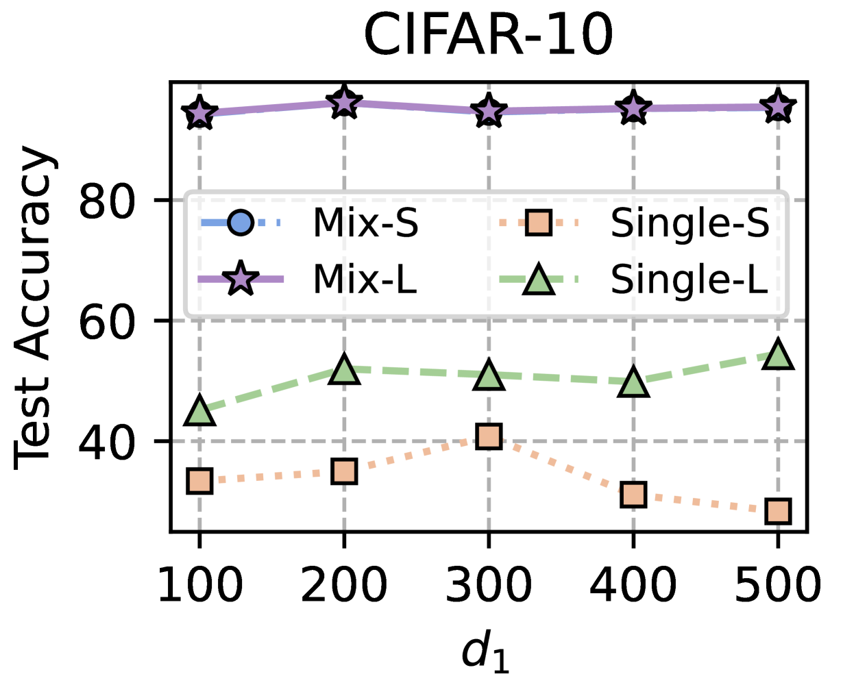<details> <summary>x23.png Details</summary>  ### Visual Description ## Line Graph: CIFAR-10 Test Accuracy vs. d1 Parameter ### Overview The chart compares test accuracy performance across four model configurations (Mix-S, Mix-L, Single-S, Single-L) as a function of the parameter `d1` (ranging from 100 to 500). Test accuracy is measured on a 0-100 scale, with distinct line styles and markers for each configuration. ### Components/Axes - **X-axis (d1)**: Discrete values at 100, 200, 300, 400, 500 (no intermediate points shown). - **Y-axis (Test Accuracy)**: 0-100 scale with 20-point increments. - **Legend**: Positioned at top-left, with four entries: - **Mix-S**: Blue dashed line with circle markers - **Mix-L**: Solid purple line with star markers - **Single-S**: Orange dotted line with square markers - **Single-L**: Green dash-dot line with triangle markers ### Detailed Analysis 1. **Mix-L (Purple Stars)**: - Consistently highest performance (90-93% accuracy) - Values: ~90 (d1=100), ~92 (d1=200), ~91 (d1=300), ~92 (d1=400), ~93 (d1=500) - Trend: Slight upward trajectory with minimal fluctuation 2. **Mix-S (Blue Circles)**: - Lowest performance (25-40% accuracy) - Values: ~30 (d1=100), ~35 (d1=200), ~40 (d1=300), ~30 (d1=400), ~25 (d1=500) - Trend: Initial rise to d1=300, then sharp decline 3. **Single-S (Orange Squares)**: - Mid-range performance (30-40% accuracy) - Values: ~30 (d1=100), ~35 (d1=200), ~40 (d1=300), ~30 (d1=400), ~25 (d1=500) - Trend: Mirrors Mix-S pattern but with slightly higher baseline 4. **Single-L (Green Triangles)**: - Second-highest performance (45-55% accuracy) - Values: ~45 (d1=100), ~50 (d1=200), ~52 (d1=300), ~50 (d1=400), ~55 (d1=500) - Trend: Gradual improvement peaking at d1=500 ### Key Observations - **Performance Hierarchy**: Mix-L > Single-L > Single-S ≈ Mix-S - **d1 Sensitivity**: All models show non-linear relationships with `d1`, with no clear monotonic trend - **Model Type Impact**: "Mix" configurations (Mix-S/L) underperform "Single" configurations (Single-S/L) despite similar naming conventions - **Accuracy Plateaus**: Mix-L maintains near-peak performance across all `d1` values ### Interpretation The data suggests: 1. **Model Architecture Matters**: The "L" suffix (likely denoting larger models) correlates with higher accuracy, particularly in Single-L configurations 2. **Mix vs. Single Tradeoff**: While "Mix" models might imply hybrid training approaches, they consistently underperform their "Single" counterparts 3. **d1 Optimization**: No single `d1` value optimizes all models, indicating complex parameter interactions 4. **Practical Implications**: Single-L configurations achieve ~55% accuracy at d1=500, suggesting potential for improvement through architectural refinements rather than parameter tuning alone The chart reveals fundamental differences in model efficacy that warrant deeper investigation into training methodologies and architectural choices rather than parameter optimization alone. 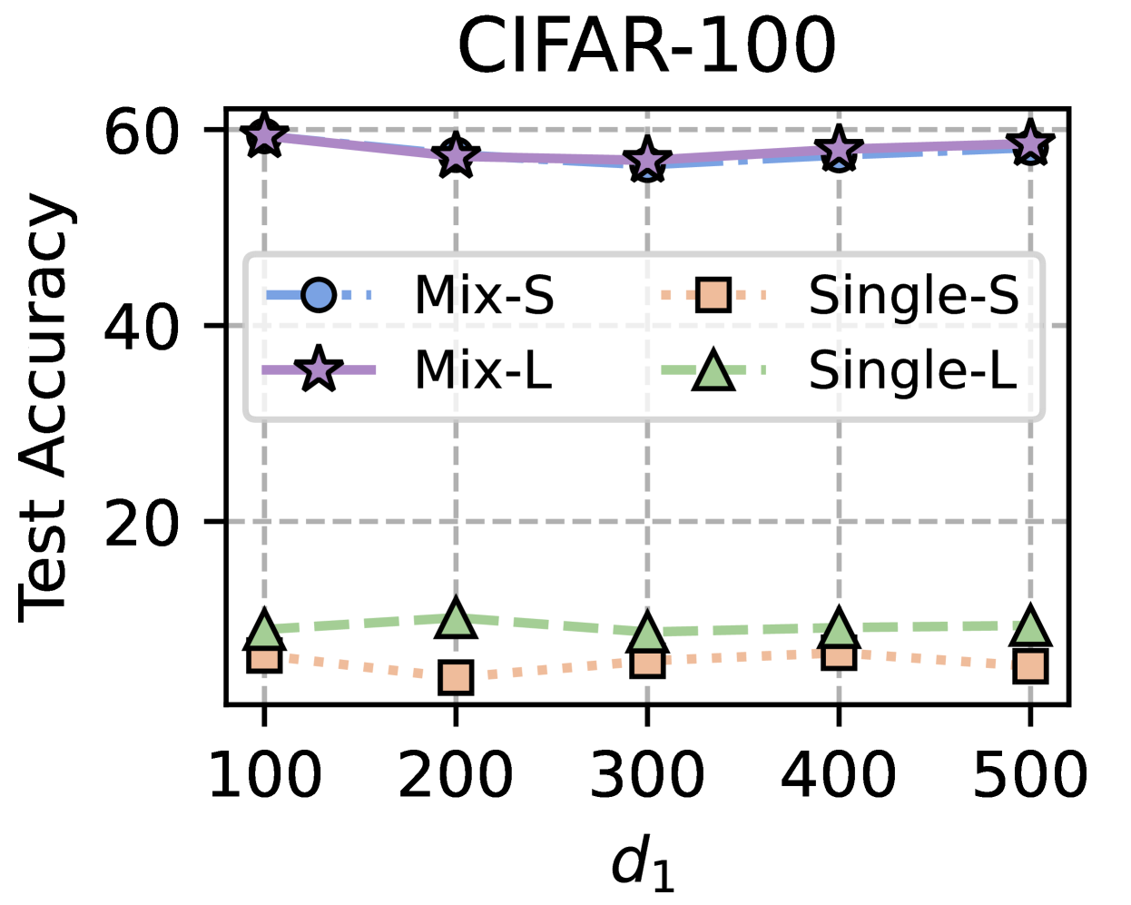</details> <details> <summary>x24.png Details</summary>  ### Visual Description ## Line Graph: CIFAR-100 Test Accuracy vs. d₁ ### Overview The graph compares test accuracy across four model configurations (Mix-S, Mix-L, Single-S, Single-L) as a function of the parameter `d₁` (ranging from 100 to 500). Test accuracy is measured on the y-axis (0–60), while `d₁` is on the x-axis. The Mix models (Mix-S and Mix-L) consistently outperform the Single models (Single-S and Single-L) across all `d₁` values. ### Components/Axes - **X-axis (d₁)**: Labeled with values 100, 200, 300, 400, 500. - **Y-axis (Test Accuracy)**: Labeled with values 0, 20, 40, 60. - **Legend**: Located at the top-right corner, with four entries: - **Mix-S**: Blue circles (dashed line). - **Mix-L**: Purple stars (solid line). - **Single-S**: Orange squares (dotted line). - **Single-L**: Green triangles (dashed-dotted line). ### Detailed Analysis 1. **Mix-S (Blue Circles)**: - Test accuracy starts at ~58 at `d₁=100`, dips to ~55 at `d₁=200`, then rises to ~57 at `d₁=500`. - Trend: Slightly fluctuating but stable around 55–58. 2. **Mix-L (Purple Stars)**: - Test accuracy starts at ~59 at `d₁=100`, dips to ~56 at `d₁=200`, then rises to ~58 at `d₁=500`. - Trend: Similar to Mix-S but slightly higher overall. 3. **Single-S (Orange Squares)**: - Test accuracy remains flat at ~10–12 across all `d₁` values. - Trend: Minimal variation, consistently low. 4. **Single-L (Green Triangles)**: - Test accuracy starts at ~12 at `d₁=100`, dips to ~10 at `d₁=200`, then rises to ~13 at `d₁=500`. - Trend: Slightly variable but remains below 15. ### Key Observations - **Performance Gap**: Mix models (S and L) achieve ~5x higher accuracy than Single models (S and L). - **Stability**: Mix models show minor fluctuations but maintain high accuracy. Single models are stable but perform poorly. - **Parameter Sensitivity**: No clear trend in accuracy improvement with increasing `d₁` for any model type. ### Interpretation The data suggests that Mix models (Mix-S and Mix-L) are significantly more effective than Single models (Single-S and Single-L) for the CIFAR-100 dataset. The minimal improvement in accuracy with increasing `d₁` implies that the parameter `d₁` may not be a critical factor for these models in this context. The consistent performance of Mix models highlights their robustness, while the flat accuracy of Single models indicates potential limitations in their architecture or training methodology. </details> Figure 7: Accuracy of four optional inference models: mix-small (the whole model without the local header), mix-large (the whole model without the global header), single-small (the homogeneous small model), single-large (the client heterogeneous model). Appendix D Discussion We discuss how FedMRL tackles heterogeneity and its privacy, communication and computation. Tackling Heterogeneity. FedMRL allows each client to tailor its heterogeneous local model according to its system resources, which addresses system and model heterogeneity. Each client achieves multi-granularity representation learning adapting to local non-IID data distribution through a personalized heterogeneous representation projector, alleviating data heterogeneity. Privacy. The server and clients communicate the homogeneous small models while the heterogeneous local model is always stored in the client. Besides, representation splicing enables the structures of the homogeneous global model and the heterogeneous local model to be not related. Therefore, the parameters and structure privacy of the heterogeneous client model is protected strongly. Meanwhile, the local data are always stored in clients for local training, so local data privacy is also protected. Communication Cost. The server and clients transmit homogeneous small models with fewer parameters than the client’s heterogeneous local model, consuming significantly lower communication costs in one communication round compared with transmitting complete local models like FedAvg. Computational Overhead. Except for training the client’s heterogeneous local model, each client also trains the homogeneous global small model and a lightweight representation projector which have far fewer parameters than the heterogeneous local model. The computational overhead in one training round is slightly increased. Since we design personalized Matryoshka Representations learning adapting to local data distribution from multiple perspectives, the model learning capability is improved, accelerating model convergence and consuming fewer training rounds. Therefore, the total computational cost may also be reduced. Appendix E Broader Impacts and Limitations Broader Impacts. FedMRL improves model performance, communication and computational efficiency for heterogeneous federated learning while effectively protecting the privacy of the client heterogeneous local model and non-IID data. It can be applied in various practical FL applications. Limitations. The multi-granularity embedded representations within Matryoshka Representations are processed by the global small model’s header and the local client model’s header, respectively. This increases the storage cost, communication costs and training overhead for the global header even though it only involves one linear layer. In future work, we will follow the more effective Matryoshka Representation learning method (MRL-E) [21], removing the global header and only using the local model header to process multi-granularity Matryoshka Representations simultaneously, to enable a better trade-off among model performance and costs of storage, communication and computation.