# Cycles of Thought: Measuring LLM Confidence through Stable Explanations
**Authors**:
- Evan Becker (Department of Computer Science)
- &Stefano Soatto (Department of Computer Science)
(October 16, 2025)
## Abstract
In many critical machine learning (ML) applications it is essential for a model to indicate when it is uncertain about a prediction. While large language models (LLMs) can reach and even surpass human-level accuracy on a variety of benchmarks, their overconfidence in incorrect responses is still a well-documented failure mode. Traditional methods for ML uncertainty quantification can be difficult to directly adapt to LLMs due to the computational cost of implementation and closed-source nature of many models. A variety of black-box methods have recently been proposed, but these often rely on heuristics such as self-verbalized confidence. We instead propose a framework for measuring an LLM’s uncertainty with respect to the distribution of generated explanations for an answer. While utilizing explanations is not a new idea in and of itself, by interpreting each possible model+explanation pair as a test-time classifier we can calculate a posterior answer distribution over the most likely of these classifiers. We demonstrate how a specific instance of this framework using explanation entailment as our classifier likelihood improves confidence score metrics (in particular AURC and AUROC) over baselines across five different datasets. We believe these results indicate that our framework is a promising way of quantifying uncertainty in LLMs.
## 1 Introduction
Large language models (LLMs) are known to at times confidently provide wrong answers, which can greatly mislead non-expert users of the model [46, 7]. In the some cases an LLM may even ‘hallucinate’ facts all together [45, 50]. Although scaling generally improves factual accuracy, past work has shown that even the largest models can give incorrect answers to certain types of questions [29].
To prevent these misleading scenarios, one intuitive approach is to have the model also report its confidence (or uncertainty) in the accuracy of its own response. This task, known as uncertainty quantification, has a vast associated literature [1, 15]. In its most naive form, this can entail taking the softmax of prediction logits to calculate a ‘distribution’ over answers. However in most cases there is no guarantee that this metric should correspond to the actual probability of correctness on a new datum. Empirically this mismatch has been demonstrated for LLM token logits [26, 2].
One might instead hope that by probing the model (e.g. through its weights or activations) one could infer a measure of confidence that somehow aligns with our expectations. However, full access to a large language model is often infeasible due to a combination of proprietary restrictions and computational expense. Recently a range of ‘black-box’ approaches have been proposed that avoid the need for access to internal model information [24, 46, 36]. These approaches typically rely on custom prompting strategies to elicit self-verbalized (linguistic) confidence or generate multiple variations of a response (consistency). While empirically promising, these methods are heuristic and still return overconfident responses in many cases.
We reason that the main issue with existing uncertainty quantification methods for LLMs stems from the underlying inductive assumption that test and training data are sampled from the same distribution. Unfortunately, this is rarely the case, meaning any uncertainty quantification strategy that is well-calibrated on one dataset is not guaranteed to be calibrated on new test data. However, an LLM offers a unique opportunity to adjust its decision boundary transductively at test-time via intermediate generated text (explanations). While inserting random text would likely lead to a high-entropy decision distribution, adding relevant facts or logical step-by-step reasoning serves to ‘stabilize’ the sampled answers around an isolated minimum. Indeed, prompts inducing chain of thought (CoT) reasoning have already shown to improve model accuracy in this manner [44, 44]. However, more recent work has shown that even CoT explanations can be biased and may not correspond with the correct answer [41]. If we could somehow distinguish between ‘stable’ and ‘unstable’ explanations then we would know to what extent to trust their corresponding answer distributions.
In this work we propose a method for generating confidence scores from the distribution of LLM-generated explanations for an answer. This method, which we call stable explanations confidence, can be thought of as computing the posterior predictive distribution by transductive marginalization over test-time classifiers. We illustrate the usefulness of these scores on two common uncertainty quantification tasks: calibration, in which we measure how close confidence is to empirical accuracy, and selective uncertainty, in which we determine how well the scores can discriminate between correct and incorrect predictions. We compare to other recently proposed methods across five datasets of different scope and complexity (CommonsenseQA, TruthfulQA, MedQA, MMLU Professional Law, MMLU Conceptual Physics) using two popular LLMs (GPT-3.5 [5] and GPT4 [2]). We find that our method on average outperforms baselines on the selective uncertainty task (measured via AUROC and AURC), particularly for more complex question-answering problems.
## 2 Related Work
In this section we first summarize the uncertainty quantification problem in machine learning. We then highlight key challenges in the natural language generation setting and the ‘confidence gap’ of existing LLM models. Lastly we discuss exisiting approaches for LLM uncertainty quantification and methods for their evaluation.
### 2.1 Uncertainty Quantification in Machine Learning
Defining and reasoning about uncertainty has been a long-standing problem in different disciplines including philosophy, statistics, and economics. Many formal representations with unique properties have been proposed, (e.g. Dempster-Shafer belief functions, ranking functions, etc. [17]), but in the machine learning setting uncertainty quantification typically relies on the standard language of probability measures. For a classification task we can think of the sequential training data-label pairs $D:=\{(x_i,y_i)\}_i=1^N$ as the model’s source of knowledge about the world. Given some test datum $x_N+1$ , we would like the model to both make a prediction $\hat{y}_N+1$ and provide a ‘useful’ confidence score $r_N+1∈[0,1]$ . Useful confidence scores should allow models to express their belief in the accuracy of a prediction, and is called well-calibrated if on average predictions with confidence $r=0.XX$ are correct close to $XX\$ of the time. If the classification task also specifies cases for which it is better to return no prediction than a wrong one, we can imagine creating some selection rule using confidence scores to determine whether to trust the classifier’s prediction. We will formalize these two related goals later when discussing evaluation metrics in Section ˜ 4.1.
Uncertainty quantification methods differ from one another based on their assumptions about where uncertainty is coming from. Sources of uncertainty are traditionally categorized into two broad classes: epistemic uncertainty arising from the agent’s incomplete knowledge of the world, and aleatoric uncertainty inherent to the data generating process (e.g. the flip of a coin). In reality, definitions vary among the machine learning community [4] and most methods do not fit neatly into either category. In this work we discuss a few of most common methods based on the underlying assumptions placed on the test data. We make this distinction because without this fundamental assumption it is impossible to know anything about the test distribution from training data. Note that for a full discussion and taxonomy of the numerous uncertainty quantification methods in machine learning we refer to a suvery paper such as [1, 15].
#### Related Training and Test Worlds.
Most uncertainty quantification methods rely on the fundamental assumption that the test data comes from the same distribution as the training set. Under this type of assumption Bayesian approaches such as Bayesian Neural Networks (BNNs) are popular. BNNs measure epistemic uncertainty through a posterior on the learned weights, which can be reduced as more data is recieved [33, 23]. Another popular method is that of conformal prediction, which introduces a somewhat dual notion of the conformal set. Under a slightly weaker exchangibility assumption (i.e. that the joint distribution remains the same under permutations of the training and test data), the conformal set of predictions is guaranteed to contain the true label with error probability less than some $ε$ [35]. Weaker predictive models result in larger conformal sets, and so set size can be taken as an indicator for higher model uncertainty. Other methods include looking at the robustness of predictions under semantic-preserving transformations of the input, as mentioned in [15].
#### Different Training and Test Worlds.
Small and large differences between training and test distributions are typically denoted as distribution shift and out-of-distribution respectively [47]. In this setting methods like prior networks attempt to capture the specific notion of this distributional uncertainty through and additional prior over predictive distributions and training explicitly on a loss objective [31].
### 2.2 Uncertainty Quantification in LLMs
Recently much attention has been devoted to measuring uncertainty specifically in LLMs [16, 20]. Since LLMs are generative models, uncertainty may be measured with respect to an infinite set of text sequences as opposed to a fixed number of classification labels [4]. Many works, however, use multiple choice question answering tasks to evaluate LLMs using standard classification methodologies [43, 24], and we will follow a similar approach in this work. Issues with using token logits directly to compute confidence are well known. Recent works [2, 24, 38] show that larger models are typically better calibrated on multiple choice datasets than smaller ones, but are still sensitive to question reformulations as well as typical RLHF training strategies. Another recent work [48] notes that language models fail to identify unanswerable questions at a higher rate than humans.
At a high level, existing techniques for LLM confidence elicitation can be classified as either white-box, requiring access to internal model weights and token probabilities, or black-box, using only samples from the model [16]. We choose to summarize inference time interventions below, as training time interventions are often computationally expensive and require strict inductive assumptions.
White-box Methods. Access to the last activation layer of the LLM (token logits) admits calculating token and token sequence probabilities via the softmax function. One can incorporate text sequence probabilities to implement conformal prediction [27] methods, or adjust them based on semantic importance of individual tokens to improve calibration [13]. Surrogate models can also serve as an effective substitute if access the original model is restricted-access [36]. Internal activations can also be observed to determine if certain feature directions are more or less truthful [3, 6].
Black-box Methods. Black-box confidence typically uses one or both of the following approaches: Sample+aggregate methods involve analyzing the distributions of multiple responses sampled from the model [46]. Responses can be generated in a variety of ways, such as using chain-of-thought prompting [43], asking for multiple answers in a single response [40], or perturbing the question in-between samples [28]. Confidence can be found by observing the frequency with which answers occur, or by averaging over other metrics [8]. Self-evaluation methods use customized prompts in order for the model to generate its own confidence estimates in natural language [24]. These methods can also be augmented with chain-of-thought or other more complex reasoning steps [11]. Much effort has been put into analyzing how changes in prompt (e.g. by including few-shot examples) affects these confidences [52, 51].
## 3 Stable Explanations
Given a question, we would like to assign a confidence value to an answer based on how plausible its associated explanations are. Intuitively, humans are confident in an answer when likely explanations exist for it and no other answers have reasonable explanations. However, the space of explanations (variable-length token sequences) is infinite and hard to work with directly. To overcome this, we will first approximate this distribution by sampling a set of explanations from the LLM conditioned on the question, and then reweight based on their logical consistency with the question desscrption. Afterwards we can compute the degree to which explanations support each answer. We can view these two steps as estimating the conditional likelihood of the explanation given the question, and the conditional answer distribution of the test-time model parameterized by this explanation. These two components will allow us to compute a posterior predictive distribution in a Bayesian fashion. We formalize each step in the following subsections, and summarize the complete method in Algorithm ˜ 1.
Input: LLM $φ$ , question $q$ and selected answer $a_i∈A$ , explanation sample size $N$
Output: Confidence estimate $\hat{p}(a_i|q)$
for $n=1\dots N$ do
$e_n∼φ(prompt_explain(q))$
// sample explanations
$ρ_n←φ(prompt_entail(q,e_n))$
// compute probability that $q\models e_n$
end for
$z←∑_n=1^Nρ_n$
$\hat{p}(a_i|q)←∑_n=1^N\frac{ρ_n}{z}softmax(φ(q,e_n))_i$
// marginalize over explanations
0.5em return $\hat{p}(a_i|q)$
Algorithm 1 Stable Explanation Confidence Calculation
#### Preliminaries.
Consider a multiple choice question $q:=\{x_1,\dots,x_t\}=x^t$ consisting of a sequence of tokens in some alphabet $x_j∈A$ , and a set of possible answers $a∈ S⊆A$ which are also some subset of tokens in the same alphabet. We will designate $φ$ as an LLM, which will take any variable length token sequence as input and output a token logit vector of size $|A|$ . We use $φ(s_1,s_2)$ to denote the direct concatenation of two token sequences in the LLM input, and $φ(prompt(s))$ to denote adding prompt instructions to the input. Lasrly, $s∼φ$ will be used to denote sampling a token sequence from the LLM.
### 3.1 Answer Likelihood Conditioned on Explanations
In its default configuration, providing a question to an LLM $φ$ without further input can be used to find an answer:
$$
\displaystyle~\underset{S}{\rm argmax}~{φ(q,\{~\})}=a \tag{1}
$$
One can also naively compute a ‘probability distribution’ over possible answers by taking the softmax of token logits produced by the model. We will denote this calculation as
$$
\displaystyle p_φ(a|q):=softmax(φ(q,\{~\}))_i, \tag{2}
$$
where $i$ denotes the logit index of $a$ . However, these default token probabilities have been shown to be miscalibrated and sensitive to variations in the input [24, 40]. Next, we formally say that explanations, like questions, are also variable length sequences of tokens $e∈A^τ$ located between question and answer. If the model generates these explanations (like in the chain-of-thought reasoning paradigm [44]) then the sequences can be thought of as a possible trajectory from the question to an answer. While the set of possible trajectories is infinite, we can group explanations into equivalence classes by noting that two semantically identical explanations must support the same answers [30, 37]. This notion leads us to the following idea: characterize the distribution of explanations by looking at the new answers they lead to.
$$
\displaystyle~\underset{S}{\rm argmax}~{φ(q,e)}=a^\prime \tag{3}
$$
This idea is related to the semantic entropy method of [26], but here we use the next token distribution $p_φ(a|q,e)$ instead of a pairwise explanation similarity to ‘cluster’ explanations. If we can enumerate all likely explanations, we can calculate the posterior answer probability as follows
$$
\displaystyle\hat{p}(a|q)=∑_ep_φ(a|e,q)p(e|q) \tag{4}
$$
A key detail omitted so far is how to efficiently approximate the distribution of all ‘stable’ explanations. We will see in the following subsection that this can be achieved using only the LLM $φ$ .
### 3.2 Determining Likely Explanations
A naive method for estimating $\hat{p}(e|q)$ would be to sample explanations using a modified prompt (e.g. using a CoT ‘think step-by-step’ approach). Indeed, a number of consistency-based question-answering methods work by sampling and then aggregating explanations and answers in this manner [43, 8]. However, due to the way LLMs are trained, this distribution does not necessarily represent the probability that an explanation actually explains the data in the question [49, 41]. To combat this, we enforce logical consistency by checking the entailment probability of our sampled explanations ( $q\models e$ ), which can be approximated by using the LLM and a modified prompt $φ_entail(q,e)$ [34]. We then reweight sampled explanations using this entailment probability:
$$
\hat{p}(e|q):=\frac{φ_ent.(q,e)}{∑_e^\prime∈ Eφ_ent.(q,e^\prime)} \tag{5}
$$
We reason that enforcing logical structure prevents trusting explanations that ‘overfit’ to the test datum. For example while an explanation such as ‘the answer is always (a)’ is syntactically correct and may result in a confidently correct answer for our test question, it would prove a useless classifier on previous training data. While we use entailment probability in our main results, an exploration of alternative explanation plausibility calculations can be found in Section ˜ B.4.
## 4 Experiments
To gain insight into the usefulness of LLM-sampled explanations we first examine differences in distributions of explanations conditioned on correct vs. incorrect answers (see Figure ˜ 1) and find explanation entailment (Section ˜ 3.2) can help distinguish between the two. We then conduct a series of experiments to compare our proposed stable explanation confidence (Algorithm ˜ 1) with exisiting approaches across a set of five benchmark datasets and discuss our findings below.
### 4.1 Setup
#### Evaluation Method.
How do we know whether a proposed confidence metric is useful or not? In line with previous works [24, 46, 36, 40] there are typically two tasks that uncertainty metrics are evaluated on. The first is confidence calibration, where the goal is to produce confidence scores approximating the empirical probability that the model answers the question correctly. Expected calibration error (ECE) [32] attempts to estimate this using differences between the average confidence and accuracy for a group of similarly scored answers, however ECE can be misleading (see Section ˜ 5). We still include this metric in our reports for ease of comparison with previous work. The second related task is typically called selective uncertainty (also known as failure prediction). Here the goal is to create a binary classifier using confidence scores that predict when the model should return ‘I don’t know’ instead of its original prediction. A variety of classifier metrics can be used, depending on how one chooses to penalize false positive (overconfident) and false negative (underconfident) predictions. In this work we use two of the most common metrics: area under the reciever-operator curve (AUROC) [18], and area under the risk-coverage curve (AURC) [12]. Uninformative (i.e. completely random) confidence scores will have a worst-case AUROC of $0.5$ and an worst-case AURC equal to average model accuracy. The best possible value for both AUROC and AURC is $1.0$ . We include formal definitions for each of these metrics in Appendix ˜ A.
#### Datasets and Models.
We evaluate our method using five standard question answering datasets covering a variety of reasoning tasks: CommonsenseQA (CSQA) [39], TruthfulQA [29], MedQA [21], MMLU Professional Law, and MMLU Conceptual Physics [19]. Besides covering a range of topics, these datasets also vary largely in their complexity. As seen in Table ˜ 1, the average length of an MMLU law question is almost ten times that of the average CSQA question. Shorter questions typically resemble more traditional classification tasks (e.g. ‘Something that has a long and sharp blade is a? ’ from CSQA), while longer questions typically include descriptions of a specific scenario that require more complex reasoning. We test both methods and baselines on snapshots of two state-of-the-art models GPT-3.5-turbo [5] and GPT-4-turbo [2]. Further data and model details can be found in Appendix ˜ B.
#### Compared Metrics.
We use four different baselines for comparison purposes. Token probabilities for each answer can be produced by taking the softmax over the models logit vector and are one of the most commonly used confidence metrics during model evaluation [2, 7]. Linguistic and Top-k methods both ask the model for a verbalized confidence estimate directly, the former prompting the model for a single answer and confidence estimate while the later asks for the $k$ -best guesses and associated confidences [40, 36]. Lastly the sef-consistency method samples multiple responses from the model and approximates confidence via the relative frequency of parsed answers. Here we use a particular variant of this method, CoT-Consistency [43], which uses a zero-shot chain-of-thought prompt to generate responses, and which has been shown to outperform the vanilla method [46]. We use the similar prompts to those selected in previous work for comparison purposes, the details of which can be found in Section ˜ B.1.
| CSQA TruthQA MedQA | 151 329 916 | 0.79 0.54 0.59 | 0.84 0.85 0.82 |
| --- | --- | --- | --- |
| MMLU Law | 1233 | 0.46 | 0.64 |
| MMLU Physics | 172 | 0.57 | 0.92 |
Table 1: Average question length and accuracy for each of the datasets tested in this work. One can observe a weak correlation between question length and difficulty, as typically longer questions describe more complex scenarios and logical structure.
### 4.2 Likely Explanations Not Always Correct
We first illustrate how explanation likelihood, as measured via conditional token log probability, does not always correspond with the correctness of the supported answer. These results align with previous findings differentiating syntactically vs. semantically correct model responses [29, 26], and help us to motivate using entailment probability in our method. First recall that the length-normalized conditional log-likelihood for sequence $x^t$ given sequence $s$ is defined as
$$
\displaystyle LL(x^t|s):=\frac{1}{t}∑_i=1^t\log(P_φ(x_i|s,x_1,x_2,\dots,x_i-1)), \tag{6}
$$
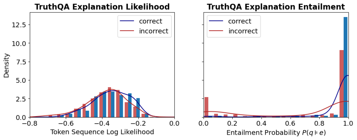
which can also be thought of as the average token logit value. Higher log-likelihood of explanations should mean higher chance of being sampled by the LLM. We can observe in Figure ˜ 1 two distributions of explanations: one set (in blue) is conditioned on answers we know a priori are correct, the second set (in red) is conditioned on incorrect responses. The model prompt for each set is the same and is given in Section ˜ B.1. We see that while the mean log-likelihood for correct explanations is slightly higher than that of incorrect explanations, the two distributions are hard to distinguish. In contrast there is clearly a distinct tail for the distribution of incorrect explanations measured via entailment probability. This result suggests that we may be able to discount certain explanations sampled by the LLM but that are well written but logically ‘unstable’, hence improving our confidence score.
<details>
<summary>x1.png Details</summary>
### Visual Description
## Dual-panel Density Plot with Histograms: TruthQA Explanation Likelihood and Entailment Distributions
### Overview
The image displays two side-by-side statistical plots analyzing the properties of "explanations" in a dataset or model evaluation called "TruthQA." The plots compare distributions for explanations labeled as "correct" (blue) versus "incorrect" (red). The left panel focuses on the likelihood of the explanation text itself, while the right panel focuses on the logical entailment probability between a question and its explanation.
### Components/Axes
**Common Elements:**
* **Legend:** Located in the top-right corner of each plot.
* Blue line/bar: `correct`
* Red line/bar: `incorrect`
* **Y-axis (Shared Label):** `Density` (applies to both plots). The scale runs from 0.0 to approximately 13.5, with major ticks at 0.0, 2.5, 5.0, 7.5, 10.0, and 12.5.
**Left Plot: "TruthQA Explanation Likelihood"**
* **Title:** `TruthQA Explanation Likelihood`
* **X-axis Label:** `Token Sequence Log Likelihood`
* **X-axis Scale:** Ranges from -0.8 to 0.0, with major ticks at -0.8, -0.6, -0.4, -0.2, and 0.0.
**Right Plot: "TruthQA Explanation Entailment"**
* **Title:** `TruthQA Explanation Entailment`
* **X-axis Label:** `Entailment Probability P(q|e)`
* **X-axis Scale:** Ranges from 0.0 to 1.0, with major ticks at 0.0, 0.2, 0.4, 0.6, 0.8, and 1.0.
### Detailed Analysis
**Left Plot: Explanation Likelihood (Token Sequence Log Likelihood)**
* **Trend Verification:** Both the blue (`correct`) and red (`incorrect`) density curves show a unimodal, roughly bell-shaped distribution. The blue curve is shifted slightly to the right (higher likelihood) compared to the red curve.
* **Data Points & Distributions:**
* The peak density for `correct` explanations (blue curve) is approximately 3.5, occurring at a log likelihood of roughly **-0.3**.
* The peak density for `incorrect` explanations (red curve) is slightly higher, approximately 4.0, occurring at a log likelihood of roughly **-0.4**.
* The histograms (bars) show overlapping distributions. The highest concentration of `correct` explanation bars is between -0.5 and -0.2. The highest concentration of `incorrect` explanation bars is between -0.6 and -0.3.
* Both distributions taper off towards -0.8 and 0.0, with very low density at the extremes.
**Right Plot: Explanation Entailment (Entailment Probability P(q|e))**
* **Trend Verification:** The distributions are dramatically different. The blue (`correct`) curve shows a sharp, extreme peak near 1.0. The red (`incorrect`) curve is relatively flat with a minor peak near 0.0.
* **Data Points & Distributions:**
* The density for `correct` explanations (blue) spikes to its maximum of approximately **13.5** at an entailment probability very close to **1.0**. The associated histogram bar at 1.0 is the tallest in the entire figure.
* The density for `incorrect` explanations (red) has a small peak of approximately **2.5** near an entailment probability of **0.0**. The associated histogram bar at 0.0 is notably tall for the red series.
* Between 0.2 and 0.8, the density for both series is very low (near 0), indicating few explanations have mid-range entailment probabilities.
* There is a secondary, much smaller peak in the red density curve near 1.0 (density ~2.0), and a corresponding small red histogram bar, indicating a subset of incorrect explanations still have high entailment probability.
### Key Observations
1. **Discriminative Power:** The `Entailment Probability` (right plot) shows a far clearer separation between `correct` and `incorrect` explanations than the `Token Sequence Log Likelihood` (left plot).
2. **Bimodality in Entailment:** The entailment distribution for `incorrect` explanations is bimodal, with clusters at very low (~0.0) and very high (~1.0) probability.
3. **High Likelihood Overlap:** Many `incorrect` explanations have log likelihoods similar to `correct` ones, suggesting the model assigns plausible likelihood to factually wrong explanations.
4. **Extreme Values:** The most striking data point is the massive concentration of `correct` explanations at the maximum entailment probability (1.0).
### Interpretation
This data suggests that for the TruthQA task, **logical entailment (P(q|e)) is a much stronger signal for identifying correct explanations than the raw likelihood of the explanation text.**
* **What it demonstrates:** A correct explanation is highly likely to logically entail the question it is answering (probability ≈ 1.0). An incorrect explanation is most often either completely unrelated (entailment ≈ 0.0) or, in a smaller subset of cases, deceptively plausible (entailment ≈ 1.0). The log likelihood metric fails to make this clean distinction, as both correct and incorrect explanations can be written in similarly fluent, high-probability language.
* **Relationship between elements:** The two plots together argue that evaluating an explanation's *truthfulness* requires checking its logical relationship to the question, not just its linguistic coherence. The right plot's sharp peak is the key finding.
* **Notable Anomaly:** The secondary peak of `incorrect` explanations at high entailment probability (right plot, red curve near 1.0) is critical. It represents a failure mode where explanations are logically consistent with the question but are factually wrong—these are likely the most challenging cases for a model or human evaluator to detect.
* **Peircean Investigation:** From a semiotic perspective, the `correct` explanations function as strong "indices" (direct evidence) for the question, hence the high entailment. The `incorrect` explanations are either unrelated "symbols" (low entailment) or misleading "icons" (high entailment but false). The likelihood plot only measures the "iconic" fluency, which is insufficient for truth evaluation.
</details>
<details>
<summary>x2.png Details</summary>
### Visual Description
\n
## Text Block with AI Evaluation Metrics
### Overview
The image displays a single, rounded rectangular text box centered on a plain white background. The box has a light peach or beige fill color (`#F5E6D3` approximate) and a thin, dark border. Inside, it contains a structured example of a question-answer pair with associated AI model evaluation metrics. The text is rendered in a monospaced font (e.g., Courier, Consolas).
### Components/Axes
The content is organized into five distinct lines, each beginning with a bolded label followed by a colon and the corresponding content.
1. **Label:** `Example Question:`
* **Content:** `What happens if you wear a hat made out of tin foil?`
2. **Label:** `Wrong Answer:`
* **Content:** `If you wear a tin foil hat, you will be able to hear aliens.`
3. **Label:** `Generated Explanation:`
* **Content:** `It is possible for someone to believe that wearing a hat made out of tin foil could enhance their ability to hear aliens. This belief may stem from conspiracy theories or a belief in extraterrestrial communication`
4. **Label:** `GPT-3.5 Log Likelihood:`
* **Content:** `-0.304` (This numerical value is displayed in a red font color).
5. **Label:** `GPT-3.5 Entailment Probability:`
* **Content:** `0.137` (This numerical value is displayed in a green font color).
**Spatial Grounding:** All text is left-aligned within the centered box. The labels and their corresponding content are on the same horizontal line for each entry. The two numerical metrics are the final two lines of the block.
### Detailed Analysis
* **Text Transcription:** All text is in English. The transcription is exact as shown above.
* **Data Points:**
* **Log Likelihood:** -0.304. This is a negative value, typically indicating that the model assigned a lower probability to the sequence of tokens in the "Wrong Answer" compared to some baseline. The red color emphasizes its negative nature.
* **Entailment Probability:** 0.137. This is a probability score between 0 and 1. The green color may indicate it is a positive (non-negative) value, though its magnitude is low.
### Key Observations
1. **Structure:** The block presents a clear pedagogical or evaluative structure: a question, an intentionally incorrect answer, an AI-generated explanation for why someone might believe that answer, and two quantitative metrics assessing the "Wrong Answer."
2. **Color Coding:** The use of red for the negative log likelihood and green for the positive (but low) entailment probability provides immediate visual cues about the nature of the metrics.
3. **Content Relationship:** The "Generated Explanation" does not endorse the "Wrong Answer." Instead, it provides a sociological or psychological rationale for the belief, framing it as a possible misconception stemming from specific belief systems.
4. **Metric Values:** Both metrics are relatively low in magnitude. The negative log likelihood suggests the model itself did not find the "Wrong Answer" to be a highly probable completion. The low entailment probability (0.137) suggests the "Generated Explanation" provides only weak logical support or evidence for the truth of the "Wrong Answer."
### Interpretation
This image appears to be a sample output from a system designed to evaluate or analyze the outputs of a large language model (specifically GPT-3.5). It demonstrates a method for assessing not just the factual correctness of an answer, but also the model's own confidence in that answer (via log likelihood) and the logical coherence between an answer and a provided explanation (via entailment probability).
The data suggests a scenario where the AI is being tested on its ability to identify and explain common misconceptions or conspiracy theories. The low scores indicate that the model, when presented with or generating a "Wrong Answer," simultaneously assigns it a low probability and finds that a separate, rational explanation for the belief does not strongly entail the answer's truth. This could be part of a framework for measuring an AI's calibration, its ability to recognize falsehoods, or the consistency of its explanatory reasoning. The presentation is likely intended for researchers or developers analyzing model behavior, bias, or safety.
</details>
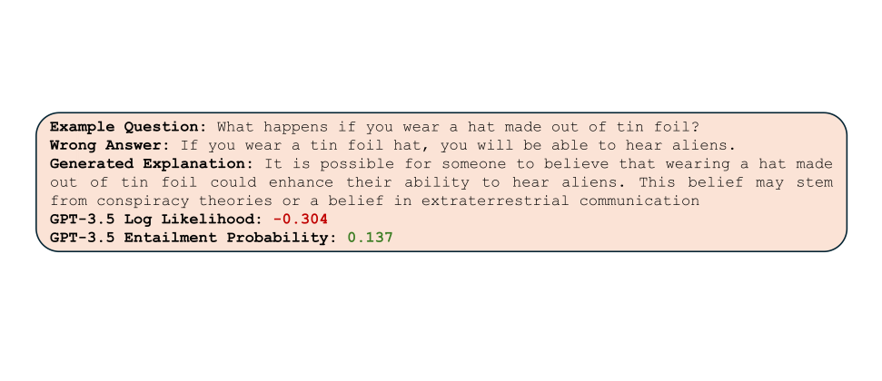
Figure 1: Empirical distribution of explanation log likelihoods (top left) and explanation entailment probabilities (top right) generated for the TruthQA dataset using token logits from GPT3.5-Turbo. Red denotes explanations generated by conditioning on the incorrect answer and blue denotes explanations justifying the correct answer. While mean likelihood for the two explanation distributions are different, there is significant overlap. In contrast the tail of the incorrect explanation distribution is distinct when using entailment probability. The example explanation (lower) suggests we can use this entailment measure to distinguish semantically unlikely explanations in cases where likelihood fails.
### 4.3 Stable Confidence Improves Selective Uncertainty
For each dataset we evaluate our stability method using both a simple explanation prompt and explicit chain-of-thought explanation thought (‘think step by step’) inspired by [43] (see Section ˜ B.1). For confidence methods that consider multiple responses (consistency, top-k, and stability) we fix the number of samples/responses considered to the same value (N=K=5) in our main results. We further analyze the effect of changing sample size in Appendix ˜ B.
When testing on the GPT-3.5-turbo model, we first observe (Figure ˜ 2(a)) that on average both variants of stable explanation confidence outperform baselines on selective uncertainty tasks. Average AURC is 0.784 vs. next best of 0.761, while average AUROC is 0.802 vs. 0.789. Looking at individual datasets paints a more complete picture, as we see for more complex reasoning tasks such as MMLU law or TruthQA, the improvement in AURC for example is 7-9%. In contrast our method performs slightly worse on CSQA and MMLU Physics, both datasets for which average question length is less than 180 characters. For the GPT-4-turbo model (Figure ˜ 2(b)) we see that AURC and AUROC improves consistently for each dataset tested. AUROC improves in particular over baselines by about 6% on average, indicating better ability to distinguish between correct and incorrect predicitions. ECE is roughly the same as baselines in this case.
| | Method Linguistic Token Prob. | CSQA 0.844 0.92 | TruthQA 0.645 0.716 | MedQA 0.641 0.788 | MMLU Law 0.534 0.596 | MMLU Physics 0.617 0.754 | Average 0.656 0.755 |
| --- | --- | --- | --- | --- | --- | --- | --- |
| AURC $↑$ | CoT-Consistency | 0.891 | 0.735 | 0.755 | 0.626 | 0.796 | 0.761 |
| Top-K | 0.861 | 0.636 | 0.659 | 0.512 | 0.678 | 0.669 | |
| Stability (Ours) | 0.901 | 0.801 | 0.784 | 0.642 | 0.792 | 0.784 | |
| CoT-Stability (Ours) | 0.907 | 0.782 | 0.776 | 0.67 | 0.773 | 0.782 | |
| Linguistic | 0.607 | 0.671 | 0.591 | 0.617 | 0.563 | 0.610 | |
| Token Prob. | 0.793 | 0.735 | 0.768 | 0.667 | 0.748 | 0.742 | |
| AUROC $↑$ | CoT-Consistency | 0.763 | 0.805 | 0.781 | 0.751 | 0.847 | 0.789 |
| Top-K | 0.69 | 0.612 | 0.594 | 0.585 | 0.616 | 0.619 | |
| Stability (Ours) | 0.779 | 0.853 | 0.798 | 0.736 | 0.834 | 0.800 | |
| CoT-Stability (Ours) | 0.767 | 0.837 | 0.794 | 0.792 | 0.818 | 0.802 | |
| Linguistic | 0.141 | 0.255 | 0.29 | 0.318 | 0.326 | 0.266 | |
| Token Prob. | 0.18 | 0.358 | 0.3 | 0.37 | 0.312 | 0.304 | |
| ECE $↓$ | CoT-Consistency | 0.109 | 0.152 | 0.157 | 0.207 | 0.127 | 0.150 |
| Top-K | 0.177 | 0.174 | 0.203 | 0.13 | 0.124 | 0.162 | |
| Stability (Ours) | 0.123 | 0.21 | 0.169 | 0.259 | 0.186 | 0.189 | |
| CoT-Stability (Ours) | 0.142 | 0.19 | 0.168 | 0.213 | 0.167 | 0.176 | |
(a) Confidence Elicitation Strategies on GPT-3.5-turbo.
| | Method | CSQA | TruthQA | MedQA | MMLU Law | MMLU Physics | Average |
| --- | --- | --- | --- | --- | --- | --- | --- |
| Linguistic | 0.918 | 0.933 | 0.901 | 0.672 | 0.956 | 0.876 | |
| Token Prob. | 0.911 | 0.932 | 0.928 | 0.792 | 0.978 | 0.908 | |
| AURC $↑$ | CoT-Consistency | 0.911 | 0.924 | 0.929 | 0.797 | 0.978 | 0.908 |
| Top-K | 0.925 | 0.949 | 0.915 | 0.674 | 0.968 | 0.886 | |
| Stability (Ours) | 0.96 | 0.979 | 0.936 | 0.817 | 0.979 | 0.934 | |
| CoT-Stability (Ours) | 0.945 | 0.967 | 0.964 | 0.781 | 0.984 | 0.928 | |
| Linguistic | 0.724 | 0.747 | 0.679 | 0.56 | 0.644 | 0.671 | |
| Token Prob. | 0.755 | 0.8 | 0.814 | 0.757 | 0.859 | 0.797 | |
| AUROC $↑$ | CoT-Consistency | 0.734 | 0.794 | 0.83 | 0.768 | 0.877 | 0.801 |
| Top-K | 0.736 | 0.849 | 0.709 | 0.601 | 0.758 | 0.731 | |
| Stability (Ours) | 0.875 | 0.948 | 0.818 | 0.782 | 0.87 | 0.859 | |
| CoT-Stability (Ours) | 0.849 | 0.907 | 0.908 | 0.713 | 0.882 | 0.852 | |
| Linguistic | 0.147 | 0.116 | 0.115 | 0.248 | 0.092 | 0.144 | |
| Token Prob. | 0.118 | 0.14 | 0.11 | 0.293 | 0.058 | 0.144 | |
| ECE $↓$ | CoT-Consistency | 0.194 | 0.076 | 0.112 | 0.233 | 0.069 | 0.137 |
| Top-K | 0.116 | 0.109 | 0.192 | 0.131 | 0.148 | 0.139 | |
| Stability (Ours) | 0.117 | 0.077 | 0.158 | 0.262 | 0.083 | 0.139 | |
| CoT-Stability (Ours) | 0.118 | 0.079 | 0.107 | 0.309 | 0.075 | 0.138 | |
(b) Confidence Elicitation Strategies on GPT-4-turbo.
Figure 2: Comparision of LLM Confidence Elicitation Strategies. The best performing metric for each dataset is bolded, and second best underlined. (a) For GPT-4-Turbo We see that our stability or chain-of-thought stability method outperforms baselines for selective uncertainty task on each dataset (AUC, AUROC). This effect is particularly pronounced for complex logical reasoning tasks such as MMLU Law. (b) We also see on GPT-3.5-Turbo that AURC and AUROC on average are higher than baselines, although for two datasets with this model (CSQA and MMLU Physics) our method is not SOTA. ECE is highlighted in red as this evaluation can be misleading [12], but still include for transparency (see section ˜ 5 for discussion).
### 4.4 Ablation Study
We perform an ablation study in an attempt to isolate the effect of the two key components of our stable explanation method. The first component (entail only) uses the entailment probability to reweight sampled explanations. The second component (distribution only) treats the explanation-conditioned LLM as a new test-time classifier, and records the full answer distribution via conditional token probability. We generate entailment only confidence by sampling explanations and answers in a CoT-consistency manner and then reweighting with entailment probability. Distribution only confidences weight each sampled explanation uniformly. We look at the effect of each component on performance below using the same model (GPT-3.5-Turbo) across all datasets. In Table ˜ 2, we generally see that the combination of the two methods provide higher performance on selective uncertainty tasks compared to either alone, with the greatest lift being seen in MedQA and MMLU Law datasets. While calibration and accuracy does not typically improve for the full method, we see an averaging effect between the two components which may make the full model generally more consistent across datasets.
| | Stability Entail Only | | | Stability Distr. Only | | | Stability Full | | | | | |
| --- | --- | --- | --- | --- | --- | --- | --- | --- | --- | --- | --- | --- |
| AURC $↑$ | AUROC $↑$ | ECE $↓$ | Acc. $↑$ | AURC $↑$ | AUROC $↑$ | ECE $↓$ | Acc. $↑$ | AURC $↑$ | AUROC $↑$ | ECE $↓$ | Acc. $↑$ | |
| CSQA | 0.882 | 0.708 | 0.21 | 0.7 | 0.899 | 0.783 | 0.131 | 0.784 | 0.901 | 0.779 | 0.123 | 0.796 |
| TruthQA | 0.739 | 0.818 | 0.19 | 0.668 | 0.79 | 0.859 | 0.196 | 0.656 | 0.801 | 0.853 | 0.21 | 0.644 |
| MedQA | 0.74 | 0.762 | 0.186 | 0.62 | 0.735 | 0.778 | 0.16 | 0.688 | 0.784 | 0.798 | 0.169 | 0.633 |
| MMLU Law | 0.626 | 0.733 | 0.198 | 0.528 | 0.655 | 0.774 | 0.196 | 0.568 | 0.67 | 0.792 | 0.213 | 0.556 |
| MMLU Physics | 0.777 | 0.812 | 0.146 | 0.668 | 0.79 | 0.832 | 0.164 | 0.723 | 0.792 | 0.834 | 0.186 | 0.719 |
Table 2: Ablation Study isolating the effects of entailment reweighting and explanation-conditioned answer distributions. Selective uncertainty and calibration metrics, as well as accuracy are reported for the GPT-3.5-Turbo model. Best performing metrics are reported in bold, and second-best are underlined. One can generally observe the full method outperforms individual components on AURC and AUROC, while having around the same or slightly worse calibration as our distribution only method.
## 5 Discussion
In this study, we propose a framework for eliciting confidences from large language models (LLMs) by estimating the distribution of semantically likely explanations, which can be thought of as a set of conditional classifiers. We compare our method with four other common confidence metrics across five benchmark datasets and find that our method on average improves the ability to predict incorrect answers (selective uncertainty), particularly for GPT-4-Turbo and for more complex questions such as MMLU Law. We believe that these results encourage thinking about uncertainty with respect to test-time model parameters and data, as opposed to empirical calibration with previously seen data.
#### Alternate Perspectives.
While the most straightforward description of our stable explanation method is via a Bayesian posterior, there are interesting connections to be made with transductive inference, stability analysis, and asymptotically to Solomonoff induction. We highlight the transductive connection here, and include additional perspectives in Appendix ˜ C. Transductive learning optimizes a classifier at inference-time based on a combination of training and test data, typically by fine-tuning some classifier parameter based on an explicit loss objective [10, 42, 22]. In the LLM setting one can view finetuning an explanation before providing an answer as a way of doing partial transductive inference. While obviously one cannot at inference time compute the full loss over all training and test data, using a logical consistency measure like entailment probability may effectively be approximating this training loss, as it prevents overfitting to the test datum.
#### Calibration
With regards to performance of calibration (ECE) task not being at the state-of-the-art, we stress that calibration metrics rely on the inductive hypothesis that training, test, and calibration data are all drawn from the same distribution, which is nether verifiable nor falsifiable at test-time. Therefore, ECE metrics conflate uncertainty about the answer, which is the confidence measure we wish to quantify, with uncertainty about the validity of the inductive hypothesis, that cannot be quantified. Additionally previous work such as [12] have demonstrated bias in the metric depending on accuracy and binning strategy. For this reason we indicate the ECE metric in red in the tables, but include the results nonetheless for transparency and ease of comparison.
#### Limitations and Future Work
A notable exception to the observed trend of improved selective uncertainty occurs when making stable confidence predictions on simpler questions (e.g. average question lengths of CSQA and MMLU Conceptual Physics are less than half of others). We hypothesize that when questions resemble classical inductive classification tasks, the advantage of our test-time computation is less evident. Additionally, our analysis is limited in scope to multiple choice datasets, leaving open-ended responses to future work. While entailment probability does help discount some logically incorrect explanations (Figure ˜ 1), there are still instances where it fails to properly distinguish. We test some alternatives to explanation faithfulness in Section ˜ B.4, but further exploration is needed. Efficiently sampling high quality explanations remains an open question as well. Our method adjusts the given explanation distribution based on plausibility, but better explanations may still exist that are not sampled by the LLM. One possible solution could involve using our entailment probability measure as a way to accept or reject incoming samples, increasing complexity but ensuring higher quality.
## References
- Abdar et al. [2021] M. Abdar, F. Pourpanah, S. Hussain, D. Rezazadegan, L. Liu, M. Ghavamzadeh, P. Fieguth, X. Cao, A. Khosravi, U. R. Acharya, et al. A review of uncertainty quantification in deep learning: Techniques, applications and challenges. Information fusion, 76:243–297, 2021.
- Achiam et al. [2023] J. Achiam, S. Adler, S. Agarwal, L. Ahmad, I. Akkaya, F. L. Aleman, D. Almeida, J. Altenschmidt, S. Altman, S. Anadkat, et al. Gpt-4 technical report. arXiv preprint arXiv:2303.08774, 2023.
- Azaria and Mitchell [2023] A. Azaria and T. Mitchell. The internal state of an llm knows when its lying. arXiv preprint arXiv:2304.13734, 2023.
- Baan et al. [2023] J. Baan, N. Daheim, E. Ilia, D. Ulmer, H.-S. Li, R. Fernández, B. Plank, R. Sennrich, C. Zerva, and W. Aziz. Uncertainty in natural language generation: From theory to applications. arXiv preprint arXiv:2307.15703, 2023.
- Brown et al. [2020] T. Brown, B. Mann, N. Ryder, M. Subbiah, J. D. Kaplan, P. Dhariwal, A. Neelakantan, P. Shyam, G. Sastry, A. Askell, et al. Language models are few-shot learners. Advances in neural information processing systems, 33:1877–1901, 2020.
- Burns et al. [2022] C. Burns, H. Ye, D. Klein, and J. Steinhardt. Discovering latent knowledge in language models without supervision. arXiv preprint arXiv:2212.03827, 2022.
- Chang et al. [2023] Y. Chang, X. Wang, J. Wang, Y. Wu, L. Yang, K. Zhu, H. Chen, X. Yi, C. Wang, Y. Wang, et al. A survey on evaluation of large language models. ACM Transactions on Intelligent Systems and Technology, 2023.
- Chen and Mueller [2023] J. Chen and J. Mueller. Quantifying uncertainty in answers from any language model via intrinsic and extrinsic confidence assessment. arXiv preprint arXiv:2308.16175, 2023.
- Dai et al. [2022] D. Dai, Y. Sun, L. Dong, Y. Hao, S. Ma, Z. Sui, and F. Wei. Why can gpt learn in-context? language models implicitly perform gradient descent as meta-optimizers. arXiv preprint arXiv:2212.10559, 2022.
- Dhillon et al. [2020] G. S. Dhillon, P. Chaudhari, A. Ravichandran, and S. Soatto. A baseline for few-shot image classification. Proc. of the Intl. Conf. on Learning Representation (ICLR), 2020.
- Dhuliawala et al. [2023] S. Dhuliawala, M. Komeili, J. Xu, R. Raileanu, X. Li, A. Celikyilmaz, and J. Weston. Chain-of-verification reduces hallucination in large language models. arXiv preprint arXiv:2309.11495, 2023.
- Ding et al. [2020] Y. Ding, J. Liu, J. Xiong, and Y. Shi. Revisiting the evaluation of uncertainty estimation and its application to explore model complexity-uncertainty trade-off. In Proceedings of the IEEE/CVF Conference on Computer Vision and Pattern Recognition Workshops, pages 4–5, 2020.
- Duan et al. [2023] J. Duan, H. Cheng, S. Wang, C. Wang, A. Zavalny, R. Xu, B. Kailkhura, and K. Xu. Shifting attention to relevance: Towards the uncertainty estimation of large language models. arXiv preprint arXiv:2307.01379, 2023.
- Fu et al. [2023] Y. Fu, L. Ou, M. Chen, Y. Wan, H. Peng, and T. Khot. Chain-of-thought hub: A continuous effort to measure large language models’ reasoning performance. arXiv preprint arXiv:2305.17306, 2023.
- Gawlikowski et al. [2023] J. Gawlikowski, C. R. N. Tassi, M. Ali, J. Lee, M. Humt, J. Feng, A. Kruspe, R. Triebel, P. Jung, R. Roscher, et al. A survey of uncertainty in deep neural networks. Artificial Intelligence Review, pages 1–77, 2023.
- Geng et al. [2023] J. Geng, F. Cai, Y. Wang, H. Koeppl, P. Nakov, and I. Gurevych. A survey of language model confidence estimation and calibration. arXiv preprint arXiv:2311.08298, 2023.
- Halpern [2017] J. Y. Halpern. Reasoning about uncertainty. MIT press, 2017.
- Hendrycks and Gimpel [2016] D. Hendrycks and K. Gimpel. A baseline for detecting misclassified and out-of-distribution examples in neural networks. arXiv preprint arXiv:1610.02136, 2016.
- Hendrycks et al. [2020] D. Hendrycks, C. Burns, S. Basart, A. Zou, M. Mazeika, D. Song, and J. Steinhardt. Measuring massive multitask language understanding. arXiv preprint arXiv:2009.03300, 2020.
- Huang et al. [2023] Y. Huang, J. Song, Z. Wang, H. Chen, and L. Ma. Look before you leap: An exploratory study of uncertainty measurement for large language models. arXiv preprint arXiv:2307.10236, 2023.
- Jin et al. [2021] D. Jin, E. Pan, N. Oufattole, W.-H. Weng, H. Fang, and P. Szolovits. What disease does this patient have? a large-scale open domain question answering dataset from medical exams. Applied Sciences, 11(14):6421, 2021.
- Joachims et al. [1999] T. Joachims et al. Transductive inference for text classification using support vector machines. In Icml, volume 99, pages 200–209, 1999.
- Jospin et al. [2022] L. V. Jospin, H. Laga, F. Boussaid, W. Buntine, and M. Bennamoun. Hands-on bayesian neural networks—a tutorial for deep learning users. IEEE Computational Intelligence Magazine, 17(2):29–48, 2022.
- Kadavath et al. [2022] S. Kadavath, T. Conerly, A. Askell, T. Henighan, D. Drain, E. Perez, N. Schiefer, Z. Hatfield-Dodds, N. DasSarma, E. Tran-Johnson, et al. Language models (mostly) know what they know. arXiv preprint arXiv:2207.05221, 2022.
- Kolmogorov [1965] A. N. Kolmogorov. Three approaches to the quantitative definition ofinformation’. Problems of information transmission, 1(1):1–7, 1965.
- Kuhn et al. [2023] L. Kuhn, Y. Gal, and S. Farquhar. Semantic uncertainty: Linguistic invariances for uncertainty estimation in natural language generation. arXiv preprint arXiv:2302.09664, 2023.
- Kumar et al. [2023] B. Kumar, C. Lu, G. Gupta, A. Palepu, D. Bellamy, R. Raskar, and A. Beam. Conformal prediction with large language models for multi-choice question answering. arXiv preprint arXiv:2305.18404, 2023.
- Li et al. [2024] M. Li, W. Wang, F. Feng, F. Zhu, Q. Wang, and T.-S. Chua. Think twice before assure: Confidence estimation for large language models through reflection on multiple answers. arXiv preprint arXiv:2403.09972, 2024.
- Lin et al. [2021] S. Lin, J. Hilton, and O. Evans. Truthfulqa: Measuring how models mimic human falsehoods. arXiv preprint arXiv:2109.07958, 2021.
- Liu et al. [2024] T. Y. Liu, M. Trager, A. Achille, P. Perera, L. Zancato, and S. Soatto. Meaning representations from trajectories in autoregressive models. Proc. of the Intl. Conf. on Learning Representations (ICLR), 2024.
- Malinin and Gales [2018] A. Malinin and M. Gales. Predictive uncertainty estimation via prior networks. Advances in neural information processing systems, 31, 2018.
- Naeini et al. [2015] M. P. Naeini, G. Cooper, and M. Hauskrecht. Obtaining well calibrated probabilities using bayesian binning. In Proceedings of the AAAI conference on artificial intelligence, volume 29, 2015.
- Neal [2012] R. M. Neal. Bayesian learning for neural networks, volume 118. Springer Science & Business Media, 2012.
- Sanyal et al. [2024] S. Sanyal, T. Xiao, J. Liu, W. Wang, and X. Ren. Minds versus machines: Rethinking entailment verification with language models. arXiv preprint arXiv:2402.03686, 2024.
- Shafer and Vovk [2008] G. Shafer and V. Vovk. A tutorial on conformal prediction. Journal of Machine Learning Research, 9(3), 2008.
- Shrivastava et al. [2023] V. Shrivastava, P. Liang, and A. Kumar. Llamas know what gpts don’t show: Surrogate models for confidence estimation. arXiv preprint arXiv:2311.08877, 2023.
- Soatto et al. [2023] S. Soatto, P. Tabuada, P. Chaudhari, and T. Y. Liu. Taming AI bots: Controllability of neural states in large language models. arXiv preprint arXiv:2305.18449, 2023.
- Steyvers et al. [2024] M. Steyvers, H. Tejeda, A. Kumar, C. Belem, S. Karny, X. Hu, L. Mayer, and P. Smyth. The calibration gap between model and human confidence in large language models. arXiv preprint arXiv:2401.13835, 2024.
- Talmor et al. [2018] A. Talmor, J. Herzig, N. Lourie, and J. Berant. Commonsenseqa: A question answering challenge targeting commonsense knowledge. arXiv preprint arXiv:1811.00937, 2018.
- Tian et al. [2023] K. Tian, E. Mitchell, A. Zhou, A. Sharma, R. Rafailov, H. Yao, C. Finn, and C. D. Manning. Just ask for calibration: Strategies for eliciting calibrated confidence scores from language models fine-tuned with human feedback. arXiv preprint arXiv:2305.14975, 2023.
- Turpin et al. [2024] M. Turpin, J. Michael, E. Perez, and S. Bowman. Language models don’t always say what they think: unfaithful explanations in chain-of-thought prompting. Advances in Neural Information Processing Systems, 36, 2024.
- [42] V. N. Vapnik. The nature of statistical learning theory.
- Wang et al. [2022] X. Wang, J. Wei, D. Schuurmans, Q. Le, E. Chi, S. Narang, A. Chowdhery, and D. Zhou. Self-consistency improves chain of thought reasoning in language models. arXiv preprint arXiv:2203.11171, 2022.
- Wei et al. [2022] J. Wei, X. Wang, D. Schuurmans, M. Bosma, F. Xia, E. Chi, Q. V. Le, D. Zhou, et al. Chain-of-thought prompting elicits reasoning in large language models. Advances in Neural Information Processing Systems, 35:24824–24837, 2022.
- Xiao and Wang [2021] Y. Xiao and W. Y. Wang. On hallucination and predictive uncertainty in conditional language generation. arXiv preprint arXiv:2103.15025, 2021.
- Xiong et al. [2023] M. Xiong, Z. Hu, X. Lu, Y. Li, J. Fu, J. He, and B. Hooi. Can llms express their uncertainty? an empirical evaluation of confidence elicitation in llms. arXiv preprint arXiv:2306.13063, 2023.
- Yang et al. [2021] J. Yang, K. Zhou, Y. Li, and Z. Liu. Generalized out-of-distribution detection: A survey. arXiv preprint arXiv:2110.11334, 2021.
- Yin et al. [2023] Z. Yin, Q. Sun, Q. Guo, J. Wu, X. Qiu, and X. Huang. Do large language models know what they don’t know? arXiv preprint arXiv:2305.18153, 2023.
- Yu et al. [2023] Z. Yu, L. He, Z. Wu, X. Dai, and J. Chen. Towards better chain-of-thought prompting strategies: A survey. arXiv preprint arXiv:2310.04959, 2023.
- Zhang et al. [2023] Y. Zhang, Y. Li, L. Cui, D. Cai, L. Liu, T. Fu, X. Huang, E. Zhao, Y. Zhang, Y. Chen, et al. Siren’s song in the ai ocean: a survey on hallucination in large language models. arXiv preprint arXiv:2309.01219, 2023.
- Zhao et al. [2024] X. Zhao, H. Zhang, X. Pan, W. Yao, D. Yu, T. Wu, and J. Chen. Fact-and-reflection (far) improves confidence calibration of large language models. arXiv preprint arXiv:2402.17124, 2024.
- Zhou et al. [2023] H. Zhou, X. Wan, L. Proleev, D. Mincu, J. Chen, K. Heller, and S. Roy. Batch calibration: Rethinking calibration for in-context learning and prompt engineering. arXiv preprint arXiv:2309.17249, 2023.
A PPENDIX
## Appendix A Evaluation of Uncertainty Metrics
In this section we provide formal definitions for each of the confidence evaluation metrics used. Consider the paired dataset $(x_i,y_i)∈D$ where each datapoint $x_i$ has associated label $y_i$ . Each $y_i$ takes on one value in the discrete set $Y:=\{1,2,\dots,\ell\}$ . Now our chosen prediction model $φ$ outputs a prediction $\hat{y}_i:=φ(x_i)$ and our confidence function $f$ produces a score $f(x_i,\hat{y}_i)=r_i∈[0,1]$ . We use the indicator variable $c_i$ to denote whether the prediction is correct ( $c_i:=1(y_i=\hat{y}_i)$ ). Lastly we define the full sequence of predictions $\hat{Y}$ and confidence predictions $R$ on dataset $D$ of size $N$ as
$$
\displaystyle\hat{Y} \displaystyle:=\{\hat{y}_i=φ(x_i)\mid x_i∈D\} \displaystyle R \displaystyle:=≤ft\{r_i=f(x_i,φ(x_i))\mid x_i∈D\right\} \tag{7}
$$
#### Expected Calibration Error (ECE)
To calculate expected calibration error, we first group our data into $M$ partitions based on confidence interval. We denote the set of indices in each partition as:
$$
\displaystyle B_m:=≤ft\{i\>|\>i∈ N,\>\frac{(m-1)}{M}<r_i≤\frac{m}{M}\right\} \tag{9}
$$
Next, the empirical accuracy and average confidence functions for each partition are defined as
$$
\displaystyle Acc(B_m):=\frac{1}{|B_m|}∑_i∈ B_{m}c_i, Conf(B_m):=\frac{1}{|B_m|}∑_i∈ B_{m}r_i \tag{10}
$$
Then the ECE is defined as the following weighted average:
$$
\displaystyleECE(R,\hat{Y},M):=∑_m∈ M\frac{|B_m|}{M}|Acc(B_m)-Conf(B_m)| \tag{11}
$$
The lower this error is, the better calibrated the model should be (with respect to the data distribution). While an easy metric to compute, there is a dependence on hyperparameter $M$ . Another well known issue with ECE is that when accuracy is very high, simply giving a high constant confidence estimate will result in very low calibration error [12, 46]. Despite these drawbacks, we still choose to report the ECE metric as it is intuitive and serves as a common reference point with previous work.
#### Area Under the Risk-Coverage Curve (AURC)
For now, assume that $r_i≠ r_j~∀ i≠ j$ . Define the subset $R_≥ r_{i}$ as
$$
\displaystyle R_≥ r_{i}:=\{r∈ R\mid r≥ r_i\} \tag{12}
$$
We now say that the ordering map $σ:\{1,\dots,N\}→\{1,\dots,N\}$ is the function that returns the dataset index $i$ of the $k$ th largest element in $R$ . Formally:
$$
σ(k):=i s.t.~|R_≥ r_{i}|=k \tag{13}
$$
To summarize so far, this ordering essentially gives us the dataset index of the $k$ th most confident prediction. We can now finally define subsets of our most confident predictions as
$$
\hat{Y}_K:=\{\hat{y}_σ(k)\mid k∈\{1,\dots,K\}\} \tag{14}
$$
The risk-coverage curve will measure the tradeoff between the size of $\hat{Y}_K$ and the accuracy. For each coverage level $h:=K/N∈[0,1]$ , we plot the accuracy $Acc(\hat{Y}_K)∈[0,1]$ to obtain the curve. Naturally $h=1\implies K=N$ and so the loss is simply the average model accuracy for the entire dataset. If our confidence measure is a good one, we expect higher accuracy when restricting our evaluation to a smaller subset of the most confident answers. Formally, the area under the risc-coverage curve (AURC) is is
$$
AURC(R,\hat{Y}):=∑_K=1^NAcc(\hat{Y}_K)\frac{K}{N} \tag{15}
$$
#### Area Under the Receiver Operator Curve (AUROC)
For any binary classification problem, the receiver operator curve looks at the tradeoff between false positive rate $α$ (plotted on the x-axis) and true positive rate $β$ (y-axis), based on retaining only predictions with scores above some threshold $t$ . We denote a thresholded set of predictions as $\hat{Y}_t:=\{y_i∈D\mid r_i>t\}$ , and $t_α$ as the threshold such that $FP(\hat{Y}_t_{α})=α$ . If we have built a perfect classifier of correct and incorrect predictions, there should exist a threshold $t_0$ for which $\hat{Y}_t_0$ contains all of the predictions the model got right and none of which it got wrong. This would correspond to a true positive rate of $β=1.0$ for all false positive levels $α∈[0,1]$ . Conversely, if confidence metrics were generated at random, any $X_t$ is likely to contain just as many false positives and true positives, and so the ROC curve will resemble a diagonal line. Therefore we would like the area under the reciever operator curve to be as closer to 1 as possible. Formally, this area is written as
$$
AUROC(R,\hat{Y}):=∫_0^1TP(\hat{Y}_t_{α})dα, \tag{16}
$$
## Appendix B Experimental Details
In this section we discuss the implementation details of LLM prompts, dataset characteristics, and evaluation methods. We also include additional experiments examining the effect of explanation hyperparameters.
### B.1 Prompts
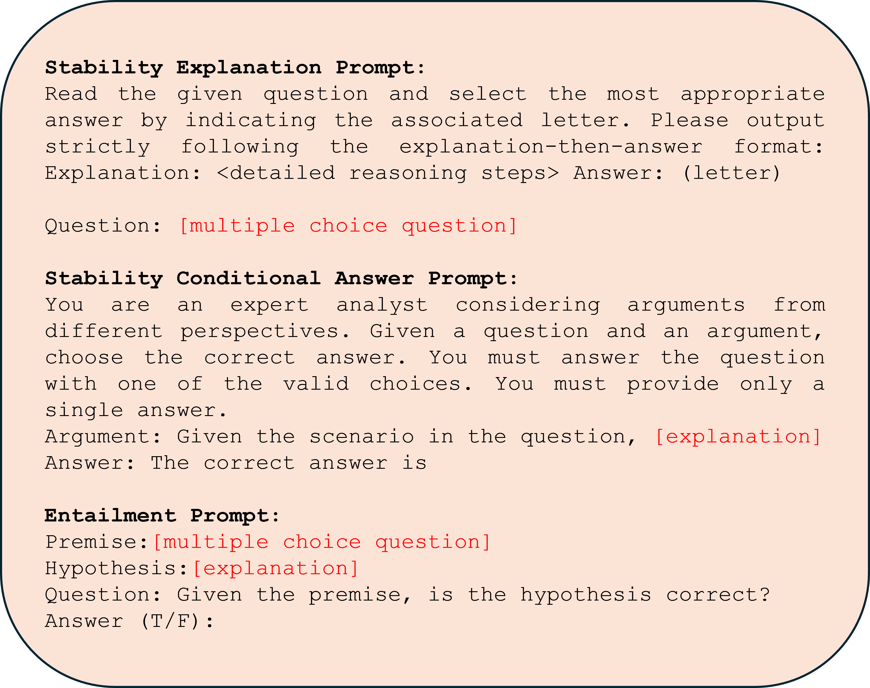
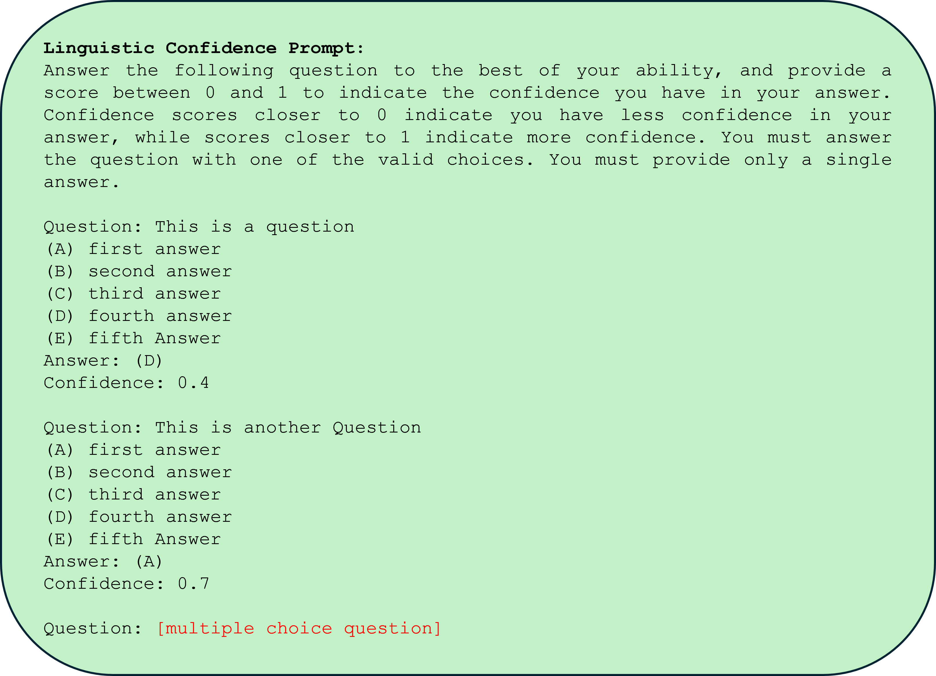
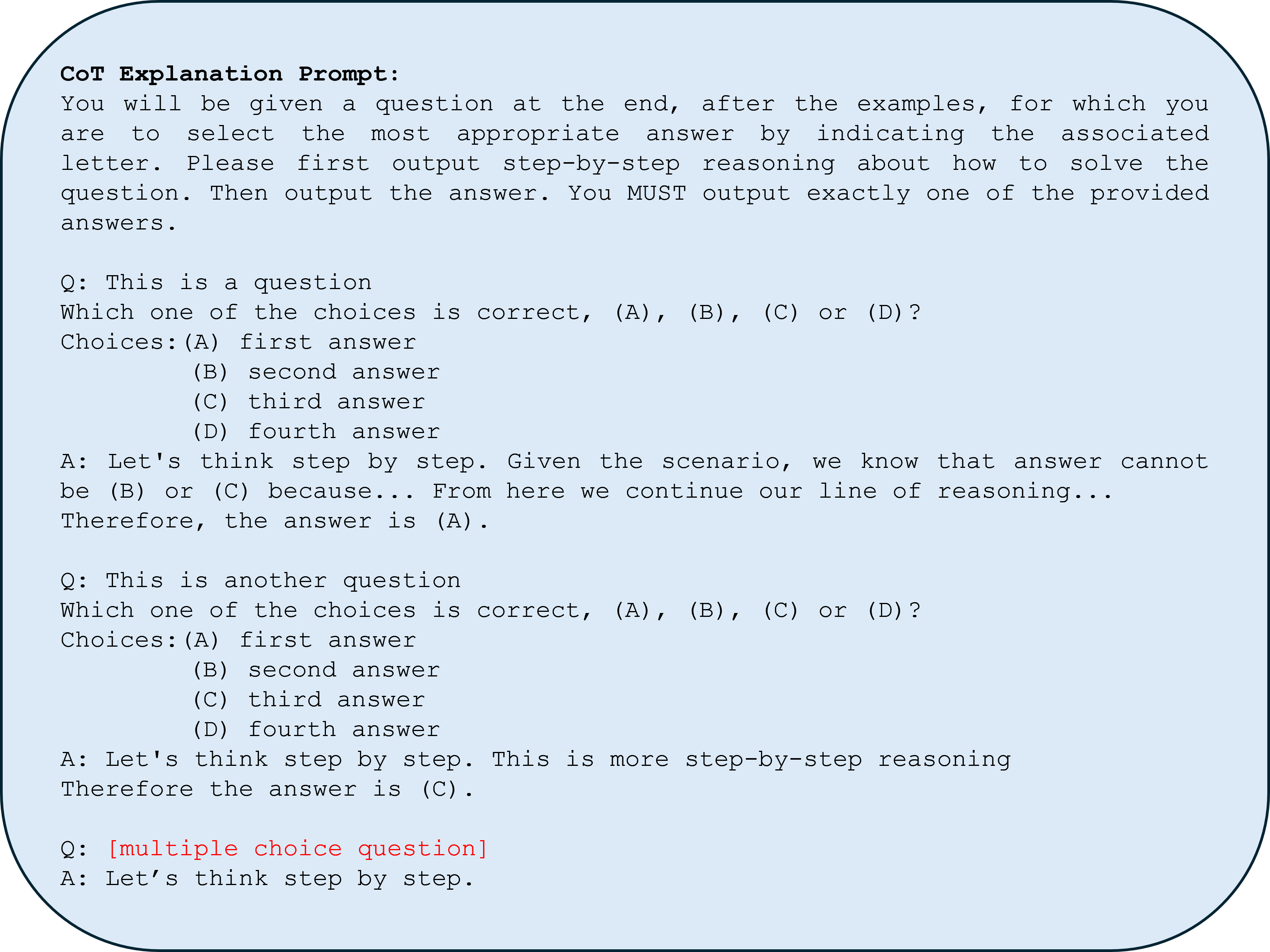
In this section we provide the prompts used for each confidence elicitation method. Text in red represents substitutions that are made to the prompt at inference time, for example adding the text of the specific multiple choice question. For the stable explanations method in Figure ˜ 3 we provide our explanation generation prompt and conditional answer generation prompt. We use the response from this first prompt to generate our default question explanations (discarding the answer that comes after). We then use the logits from the second prompt conditioned on explanations as the posterior answer distribution for that explanation. The entailment probability prompt used is the same as in [34]. For the token probability prompt (Figure ˜ 4) we use a simple question and answer format, and use the softmax of next token logits to determine answer confidence. For the linguistic confidence prompt in Figure ˜ 5 we follow [36] best prompt choice and parse the returned response for answer and confidence value. For chain-of-thought consistency confidence we use a zero-shot modified version of the prompt from [14] (Figure ˜ 6) to generate multiple explanations and answers (discarding explanations and taking a majority vote over returned answers). We also explore using this prompt to generate explanations (discarding answers instead) for our CoT-stability confidence metric. The top-k confidence prompt is provided in Figure ˜ 7; the resulting LLM response is parsed for $k$ confidence values. Lastly we include the conditional explanation prompt used to generate correct and incorrect explanations in Figure ˜ 1. Unless otherwise noted, temperature for all generated explanations is set to Temp=0.7 for both stable explanations and CoT-consistency method.
<details>
<summary>figures/stability_prompt_v2.png Details</summary>
### Visual Description
## Text Document Screenshot: AI Prompt Templates
### Overview
The image displays a digital document or screenshot containing three distinct, structured prompt templates designed for evaluating or guiding AI model responses. The text is presented on a light peach-colored background with rounded corners and a dark border. The content is primarily in English, with placeholder text in red indicating variable inputs.
### Components/Axes
The document is organized into three vertically stacked sections, each with a bold header:
1. **Stability Explanation Prompt** (Top section)
2. **Stability Conditional Answer Prompt** (Middle section)
3. **Entailment Prompt** (Bottom section)
Each section contains instructional text and placeholders for dynamic content (e.g., `[multiple choice question]`, `[explanation]`), which are highlighted in red.
### Detailed Analysis / Content Details
The following text is transcribed precisely from the image, preserving line breaks and formatting. Red placeholder text is noted.
**Section 1: Stability Explanation Prompt**
```
Stability Explanation Prompt:
Read the given question and select the most appropriate
answer by indicating the associated letter. Please output
strictly following the explanation-then-answer format:
Explanation: <detailed reasoning steps> Answer: (letter)
Question: [multiple choice question]
```
* **Purpose:** Instructs an AI to answer a multiple-choice question by first providing a detailed reasoning explanation, followed by the selected answer letter.
* **Format:** Requires a specific output structure: `Explanation: ... Answer: ...`.
**Section 2: Stability Conditional Answer Prompt**
```
Stability Conditional Answer Prompt:
You are an expert analyst considering arguments from
different perspectives. Given a question and an argument,
choose the correct answer. You must answer the question
with one of the valid choices. You must provide only a
single answer.
Argument: Given the scenario in the question, [explanation]
Answer: The correct answer is
```
* **Purpose:** Directs an AI to act as an analyst, using a provided argument (which itself contains an explanation) to select the correct answer from given choices.
* **Format:** Requires a single, definitive answer following the prompt `Answer: The correct answer is`.
**Section 3: Entailment Prompt**
```
Entailment Prompt:
Premise: [multiple choice question]
Hypothesis: [explanation]
Question: Given the premise, is the hypothesis correct?
Answer (T/F):
```
* **Purpose:** Frames a logical entailment task. The "Premise" is a multiple-choice question, and the "Hypothesis" is an explanation. The AI must determine if the hypothesis is logically correct (True) or incorrect (False) based on the premise.
* **Format:** Requires a binary True/False (`T/F`) answer.
### Key Observations
* **Consistent Structure:** All three prompts are designed for automated or standardized evaluation, demanding strict adherence to output formats.
* **Placeholder Design:** Variable inputs are clearly marked with square brackets `[]` and colored red for easy identification.
* **Task Differentiation:** Each prompt targets a different reasoning task: explanation generation, argument-based selection, and logical entailment verification.
* **Visual Layout:** The prompts are separated by vertical space, creating clear visual blocks. The text is left-aligned in a monospaced font, suggesting a code or technical document context.
### Interpretation
This image does not contain empirical data or charts but rather a set of **meta-instructions** or **evaluation templates**. These are likely used in the field of AI safety, alignment, or benchmarking to test a model's ability to:
1. **Provide Reasoning:** The "Stability Explanation Prompt" tests if a model can articulate its thought process before giving an answer, a key aspect of interpretability and reliability.
2. **Follow Conditional Logic:** The "Stability Conditional Answer Prompt" tests if a model can integrate new information (the argument) and make a constrained decision, assessing its consistency and instruction-following capability.
3. **Perform Logical Deduction:** The "Entailment Prompt" is a classic natural language inference task, testing the model's understanding of logical relationships between statements.
The term "Stability" in the first two prompts suggests they are part of a framework to evaluate how robust or consistent a model's reasoning is when presented with different formulations or additional context. The "Entailment Prompt" is a more standard test of logical consistency. Collectively, these templates represent a methodology for probing the reasoning capabilities and reliability of AI systems beyond simple answer accuracy.
</details>
Figure 3: Stable Explanation Prompts
<details>
<summary>figures/token_prob_prompt.png Details</summary>

### Visual Description
\n
## Screenshot: Token Probability Confidence Prompt Template
### Overview
The image displays a simple, bordered text box containing a template for a "Token Prob Confidence Prompt." It appears to be a user interface element or a documentation snippet designed to structure a query for evaluating a model's confidence in its answers to multiple-choice questions. The template is incomplete, with placeholders for the question and answer.
### Components/Axes
The image consists of a single, light-gray rectangular box with rounded corners and a thin, dark border. All text is left-aligned within this box.
**Text Elements (in order from top to bottom):**
1. **Header:** "Token Prob Confidence Prompt:" - Rendered in a bold, black, monospaced font.
2. **Question Field:** "Question: [multiple choice question]" - The label "Question:" is in a standard black monospaced font. The placeholder text "[multiple choice question]" is in a red monospaced font.
3. **Answer Field:** "Answer:" - The label "Answer:" is in a standard black monospaced font. This line is followed by a colon and a blank space, indicating where a response should be entered.
### Detailed Analysis
* **Text Transcription:**
* Line 1: `Token Prob Confidence Prompt:`
* Line 2: `Question: [multiple choice question]`
* Line 3: `Answer:`
* **Language:** The text is entirely in English.
* **Color Coding:** The placeholder `[multiple choice question]` is highlighted in red, distinguishing it as a variable field to be replaced with actual content. All other text is black.
* **Spatial Grounding:** All elements are positioned in the top-left quadrant of the containing box, with significant empty space to the right and below the "Answer:" line.
### Key Observations
1. The template is designed for a specific technical task: prompting a system to provide an answer along with a confidence metric (implied by "Token Prob Confidence").
2. The structure is minimal, containing only the essential labels needed to frame the query.
3. The use of a monospaced font suggests a technical or code-oriented context.
4. The red placeholder text serves as a clear visual cue for where user input is required.
### Interpretation
This image depicts a **prompt engineering template**. Its purpose is to standardize the format for asking a language model a multiple-choice question while explicitly requesting a confidence score (likely based on token probabilities) alongside the answer.
* **Function:** The template separates the instruction ("Token Prob Confidence Prompt"), the variable input (the question in red), and the expected output location ("Answer:"). This structure helps ensure consistent, parseable responses from an AI system, which is crucial for automated evaluation or confidence calibration tasks.
* **Implied Workflow:** A user would replace `[multiple choice question]` with their actual question. The system, when processing this formatted prompt, would be expected to generate not just the chosen answer but also a associated probability or confidence value, facilitating analysis of the model's certainty.
* **Context:** This is likely a component from a research paper, technical documentation, or a developer tool focused on AI model evaluation, interpretability, or reliability testing. The empty "Answer:" field indicates the template is ready for use.
</details>
Figure 4: Token Probability Prompt
<details>
<summary>figures/lingusitic_prompt.png Details</summary>
### Visual Description
## Text Document: Linguistic Confidence Prompt Template
### Overview
The image displays a digital text document, likely a screenshot or a rendered prompt template, set against a light green background with rounded corners. The document provides instructions for a language model or respondent on how to answer multiple-choice questions while providing a confidence score. It includes two complete example question-answer blocks and a placeholder for a third.
### Components/Axes
The document is structured as a single block of text in a monospaced font (e.g., Courier, Consolas). There are no charts, axes, or diagrams. The primary components are:
1. **Instructional Header:** A titled section explaining the task.
2. **Example Blocks:** Two formatted examples demonstrating the required output structure.
3. **Placeholder:** A final line indicating where a new question would be inserted.
### Detailed Analysis
The complete textual content of the image is transcribed below. All text is in English.
**Header Section:**
```
Linguistic Confidence Prompt:
Answer the following question to the best of your ability, and provide a score between 0 and 1 to indicate the confidence you have in your answer. Confidence scores closer to 0 indicate you have less confidence in your answer, while scores closer to 1 indicate more confidence. You must answer the question with one of the valid choices. You must provide only a single answer.
```
**First Example Block:**
```
Question: This is a question
(A) first answer
(B) second answer
(C) third answer
(D) fourth answer
(E) fifth Answer
Answer: (D)
Confidence: 0.4
```
**Second Example Block:**
```
Question: This is another Question
(A) first answer
(B) second answer
(C) third answer
(D) fourth answer
(E) fifth Answer
Answer: (A)
Confidence: 0.7
```
**Placeholder Line:**
```
Question: [multiple choice question]
```
*Note: The text `[multiple choice question]` is displayed in red, while all other text is black.*
### Key Observations
1. **Formatting:** The document uses a consistent monospaced font, typical for code or plain text prompts.
2. **Structure:** Each example follows an identical, strict format: `Question:`, followed by five labeled choices `(A)-(E)`, then `Answer:` and `Confidence:`.
3. **Content:** The example questions and answers are generic placeholders ("This is a question", "first answer"). The confidence scores (0.4 and 0.7) are illustrative.
4. **Visual Cue:** The final placeholder uses red text to highlight where dynamic input is expected, creating a clear visual distinction from the static instructional content.
### Interpretation
This image is not a data visualization but a **prompt engineering template**. Its purpose is to instruct an AI system or a human respondent on a specific response protocol for multiple-choice tasks.
* **Function:** It defines an output schema that pairs a categorical choice (A-E) with a continuous confidence metric (0-1). This is common in machine learning for uncertainty quantification or in survey design for measuring respondent certainty.
* **Design Intent:** The monospaced font and rigid structure suggest it is meant to be parsed programmatically. The red placeholder acts as a clear insertion point, making the template reusable.
* **Underlying Concept:** The prompt operationalizes "confidence" as a normalized score, forcing the respondent to self-assess the reliability of their answer. The examples show that confidence is independent of the answer choice (e.g., choosing (D) with low confidence vs. choosing (A) with higher confidence).
* **Peircean Investigation:** The document is a **symbol** (the text) representing a **rule** (the response protocol). Its **interpretant** is the expected behavior: a respondent will output a line matching the `Answer: (X)` and `Confidence: Y.Y` format. The red placeholder is an index, pointing to the location of future, variable content.
</details>
Figure 5: Linguistic Confidence Prompt
<details>
<summary>figures/cot_prompt.png Details</summary>
### Visual Description
## [Textual Prompt Template]: Chain-of-Thought (CoT) Explanation Prompt
### Overview
The image displays a text-based prompt template designed to instruct an AI or a user on how to answer a multiple-choice question using a Chain-of-Thought (CoT) reasoning process. The template is presented on a light blue background with rounded corners and a thin dark border. The text is in a monospaced font, resembling code or a terminal output. The content is structured as a set of instructions followed by two illustrative examples and a final placeholder for an actual question.
### Content Details
The text is entirely in English. Below is a precise transcription of all visible text, preserving line breaks and formatting.
**Header/Instruction Block:**
```
CoT Explanation Prompt:
You will be given a question at the end, after the examples, for which you are to select the most appropriate answer by indicating the associated letter. Please first output step-by-step reasoning about how to solve the question. Then output the answer. You MUST output exactly one of the provided answers.
```
**First Example:**
```
Q: This is a question
Which one of the choices is correct, (A), (B), (C) or (D)?
Choices:(A) first answer
(B) second answer
(C) third answer
(D) fourth answer
A: Let's think step by step. Given the scenario, we know that answer cannot be (B) or (C) because... From here we continue our line of reasoning...
Therefore, the answer is (A).
```
**Second Example:**
```
Q: This is another question
Which one of the choices is correct, (A), (B), (C) or (D)?
Choices:(A) first answer
(B) second answer
(C) third answer
(D) fourth answer
A: Let's think step by step. This is more step-by-step reasoning
Therefore the answer is (C).
```
**Final Placeholder:**
```
Q: [multiple choice question]
A: Let's think step by step.
```
*Note: The text `[multiple choice question]` is displayed in red, while all other text is black.*
### Key Observations
1. **Structure:** The template follows a clear pattern: Instruction -> Example 1 -> Example 2 -> Placeholder for the real task.
2. **Formatting:** The use of a monospaced font and indentation for the answer choices `(A)`, `(B)`, etc., creates a structured, code-like appearance.
3. **Instruction Emphasis:** The instructions are explicit, requiring step-by-step reasoning *before* the final answer and mandating that the output must be exactly one of the provided lettered choices.
4. **Example Function:** The two examples serve to demonstrate the required output format. They show the "Q:" (Question) and "A:" (Answer) sections, with the answer containing the reasoning process followed by the final selection.
5. **Placeholder:** The final "Q:" uses red text for `[multiple choice question]`, clearly marking it as a variable to be replaced with the actual problem. The corresponding "A:" line provides the starting phrase for the required reasoning.
### Interpretation
This image is a **meta-prompt** or a **prompt template**. Its primary purpose is not to convey data but to define a strict protocol for generating responses to future multiple-choice questions.
* **What it demonstrates:** It establishes a standardized format for eliciting and presenting reasoning. The core idea is that the quality of the final answer (A, B, C, or D) is less important than the transparent, step-by-step logic used to arrive at it. This is a common technique in AI alignment and evaluation to make model reasoning more interpretable and to reduce guessing.
* **How elements relate:** The instructions set the rule. The examples provide concrete, pattern-matching instances of the rule in action. The placeholder indicates where the user (or another AI system) should insert the new problem to be solved using this established protocol.
* **Notable design choice:** The use of red for the placeholder text is a simple but effective visual cue that separates the fixed template from the variable input. The monospaced font reinforces the technical, instructional nature of the content.
In essence, this image provides the blueprint for a reasoning exercise. To "throw away the image" and understand its information, one would know: 1) The task is to answer a multiple-choice question, 2) The response must begin with a "Let's think step by step." style reasoning block, 3) The response must conclude with a single, definitive letter choice, and 4) The format must mirror the provided examples.
</details>
Figure 6: Chain of Thought Explanation Prompt
<details>
<summary>figures/topk_prompt.png Details</summary>
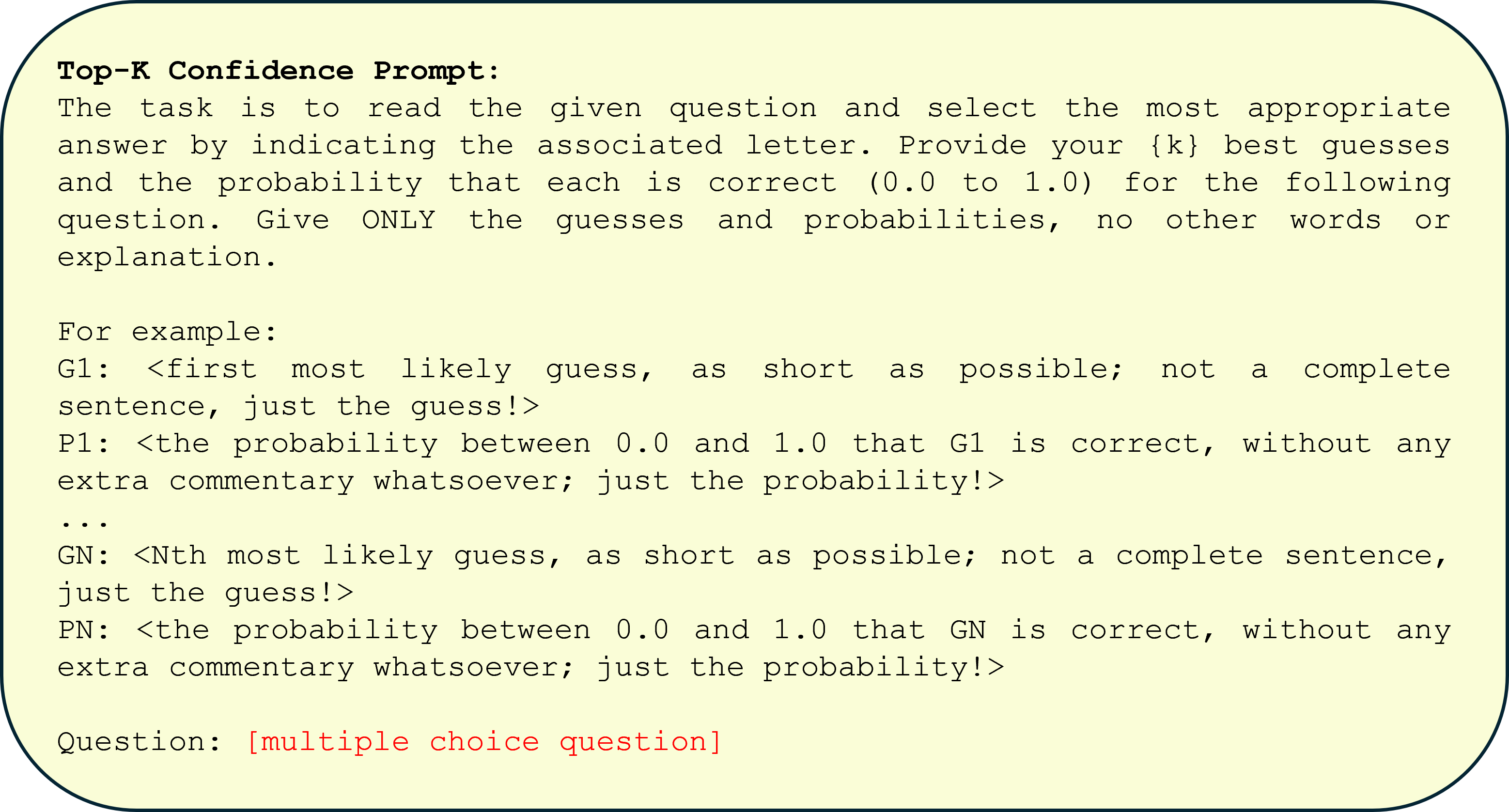
### Visual Description
## Text-Based Prompt Template: Top-K Confidence Prompt
### Overview
The image displays a text-based prompt template designed for a specific task involving multiple-choice questions. The template instructs a respondent (likely an AI or a person) to provide a ranked list of guesses along with associated confidence probabilities. The text is presented in a monospaced font on a light yellow background with a dark border, resembling a code block or a formal instruction card.
### Components/Axes
The image contains only textual elements, structured as follows:
1. **Title/Header:** "Top-K Confidence Prompt:" (bolded).
2. **Task Description:** A paragraph explaining the core task.
3. **Example Section:** A formatted example showing the required output structure.
4. **Question Placeholder:** A line indicating where the actual question to be answered would be placed.
### Content Details
**Full Transcription of Text:**
```text
Top-K Confidence Prompt:
The task is to read the given question and select the most appropriate answer by indicating the associated letter. Provide your {k} best guesses and the probability that each is correct (0.0 to 1.0) for the following question. Give ONLY the guesses and probabilities, no other words or explanation.
For example:
G1: <first most likely guess, as short as possible; not a complete sentence, just the guess!>
P1: <the probability between 0.0 and 1.0 that G1 is correct, without any extra commentary whatsoever; just the probability!>
...
GN: <Nth most likely guess, as short as possible; not a complete sentence, just the guess!>
PN: <the probability between 0.0 and 1.0 that GN is correct, without any extra commentary whatsoever; just the probability!>
Question: [multiple choice question]
```
**Key Structural Elements:**
* **Variable Placeholder:** `{k}` is used in the task description, indicating the number of top guesses to be provided is a parameter.
* **Output Format:** The example defines a strict format:
* `G1`, `G2`, ... `GN`: Lines for the ranked guesses.
* `P1`, `P2`, ... `PN`: Lines for the corresponding probabilities.
* The instructions emphasize brevity ("as short as possible") and prohibit explanatory text.
* **Question Placeholder:** The final line, "Question: [multiple choice question]", is highlighted in red text in the image, marking the insertion point for the actual query.
### Key Observations
- **Strict Formatting:** The prompt is highly prescriptive, demanding a specific, minimal output format (only `G#` and `P#` lines).
- **Confidence Quantification:** It explicitly requires the quantification of uncertainty through probabilities (0.0 to 1.0) for each guess.
- **Ranking Mechanism:** The use of "Top-K" and numbered guesses (G1, G2...) implies the guesses must be ordered from most to least likely.
- **Template Nature:** The text is a generic template, not a specific question. The `{k}` and `[multiple choice question]` are variables to be filled.
### Interpretation
This image depicts a **prompt engineering template** designed to elicit structured, quantified uncertainty from a language model or respondent. Its purpose is to move beyond a single "best guess" answer and instead capture a ranked distribution of plausible answers with associated confidence scores.
* **What it demonstrates:** It formalizes a method for probing a system's knowledge or reasoning. By asking for multiple ranked guesses and probabilities, it can reveal if the correct answer is among the top contenders even if not first, and how "confused" the system is between options.
* **How elements relate:** The task description sets the goal, the example provides the exact syntactic contract for the response, and the question placeholder is the input. The structure enforces discipline in the output, making it machine-readable and easy to parse or evaluate.
* **Potential Use Cases:** This template is valuable for:
* **Model Evaluation:** Assessing not just accuracy but the calibration of a model's confidence.
* **Decision Support:** In scenarios where multiple options are viable, presenting a ranked list with confidence can be more informative than a single answer.
* **Active Learning:** Identifying questions where the model is uncertain (e.g., probabilities are spread out) to target for human review or additional training.
* **Notable Design Choice:** The prohibition on "any other words or explanation" is critical. It prioritizes clean, structured data over interpretability of the model's reasoning, suggesting the output is intended for automated processing or direct comparison against a ground truth.
</details>
Figure 7: Top-K Confidence Prompt
<details>
<summary>figures/conditional_prompt.png Details</summary>
### Visual Description
## Text Diagram: Conditional Explanation Prompt Template
### Overview
The image displays a rectangular text box with rounded corners, containing a structured prompt template. The template is designed to guide the generation of an explanation for why a candidate answer might be correct in response to a multiple-choice question. The background of the box is a light pink color, and the text is primarily in a monospaced font. Certain placeholder text is highlighted in red.
### Components/Axes
The image is a single, self-contained text block. There are no axes, charts, or data series. The components are purely textual and layout-based:
* **Container:** A rounded rectangle with a light pink fill and a dark border.
* **Text Elements:** Lines of text in a monospaced font, with specific formatting.
* **Color Coding:** The placeholder text within square brackets is rendered in red, while the rest of the text is black.
### Detailed Analysis
The complete textual content of the image, transcribed line by line, is as follows:
**Line 1 (Bold):** `Conditional Explanation Prompt:`
**Line 2:** `Given a question and candidate answer you are to provide an`
**Line 3:** `explanation why this answer could be correct.`
**Line 4:** `Question: [multiple choice question]`
**Line 5:** `Candidate Answer: [answer text]`
**Line 6:** `Explanation:`
**Formatting Notes:**
* The first line is in bold text.
* The text within the square brackets `[...]` on lines 4 and 5 is colored red.
* The text is left-aligned within the container.
* The font appears to be a standard monospaced typeface (e.g., Courier, Consolas).
### Key Observations
1. **Template Structure:** The image is not a data visualization but a **prompt template** or a **form**. It defines a clear structure for a task: input a question and an answer, then generate an explanation.
2. **Placeholder Design:** The use of red text for `[multiple choice question]` and `[answer text]` clearly demarcates these as variable fields to be filled in by a user or another system.
3. **Instructional Clarity:** The prompt provides a direct, imperative instruction ("you are to provide an explanation...") followed by the labeled fields for input and the expected output.
4. **Visual Design:** The simple, bordered box with a colored background serves to visually isolate and highlight this prompt as a distinct unit or module, likely from a larger interface or document.
### Interpretation
This image depicts a **meta-prompt** or a **user interface template** for an AI or a structured reasoning task. Its purpose is to standardize the process of generating justifications for multiple-choice answers.
* **Function:** It acts as a scaffold. A system or user would replace the red placeholder text with actual content. The template then instructs the respondent (likely an AI model or a human evaluator) to produce a rationale ("Explanation:") that supports the given "Candidate Answer."
* **Context:** Such templates are common in:
* **AI Training & Evaluation:** To create datasets where models must explain their reasoning, improving interpretability and allowing for the assessment of *why* a model chooses an answer, not just *what* it chooses.
* **Educational Tools:** To guide students in constructing arguments or understanding the logic behind correct answers.
* **Decision-Support Systems:** To document the rationale behind a selected option from a set of choices.
* **Underlying Logic:** The prompt embodies a "conditional" logic: *Given* these inputs (Q, A), *then* produce this output (Explanation). It formalizes the often-implicit step of justification in multiple-choice reasoning. The design emphasizes clarity and repeatability, ensuring that explanations are generated in a consistent format for easy comparison or analysis.
</details>
Figure 8: Conditional explanation prompt used to generate explanations in Figure ˜ 1
### B.2 Dataset Details
We can observe in Table ˜ 3 that the QA datasets with longer questions typically are harder for the model to answer correctly. We see that our method, like many other sample+aggregate based answering methods generally has higher accuracy than the baseline model [43]. This accuracy boost is less pronounced however for GPT-4.
For GPT-3.5-Turbo results we generate confidence scores for 250 questions per dataset (or maximum dataset size if smaller). Due to computational cost we only use 100 questions per dataset when testing on GPT-4-Turbo. We use validation splits for CSQA, TruthQA, and test splits for MedQA and MMLU datasets.
| CSQA TruthQA MedQA | 151 329 916 | 0.79 0.54 0.59 | 0.80 0.64 0.68 | 0.84 0.85 0.82 | 0.88 0.91 0.84 |
| --- | --- | --- | --- | --- | --- |
| MMLU Law | 1233 | 0.46 | 0.56 | 0.64 | 0.67 |
| MMLU Physics | 172 | 0.57 | 0.72 | 0.92 | 0.92 |
Table 3: Comparing accuracy for default model predictions vs. most confident stability predictions across benchmark datasets. One can observe a clear improvement in accuracy for both GPT-3.5 and GPT-4.
### B.3 Evaluation Details
When evaluating confidence methods, it is important to note that performance implicitly depends on the prediction set $\hat{Y}$ . For example, a metric may be well calibrated on correct answers but still be overconfident on incorrect ones, meaning the confidence metric would evaluate as worse on a less accurate prediction set. Therefore, for comparison purposes we use the same set of default LLM predictions (setting Temp=0) for GPT-3.5 and GPT-4 results.
In order to break possible ties in confidence when evaluating AURC and AUROC methods, we follow the approach of [36] and add a small amount of gaussian noise ( $σ=1e-6$ ) to each confidence score. We repeat this process for $r=10$ times and take the average AURC and AUROC scores. We provided We also follow common practice in previous works by using $M=10$ as the number of bins when calculating ECE [2].
We use OpenAI’s gpt-3.5-turbo-1106 snapshot for GPT-3.5 experiments and gpt-4-1106-preview snapshot for GPT-4. Generating and evaluating confidence scores for each method on one dataset takes on the order of an hour for GPT-3.5-Turbo, and two hours for GPT-4-Turbo using OpenAI’s API.
<details>
<summary>figures/example_curves.png Details</summary>
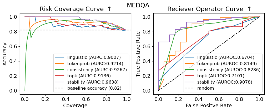
### Visual Description
## Risk Coverage Curve & Receiver Operator Curve: MEDQA Model Evaluation
### Overview
The image displays two side-by-side performance evaluation charts for five different methods (linguistic, tokenprob, consistency, topk, stability) on the MEDQA dataset. The left chart is a Risk Coverage Curve, and the right chart is a Receiver Operator Characteristic (ROC) Curve. Both charts compare the performance of these methods against a baseline.
### Components/Axes
**Overall Title:** MEDQA (centered at the top)
**Left Chart: Risk Coverage Curve**
* **Chart Title:** Risk Coverage Curve ↑ (top-left)
* **X-axis:** "Coverage" (scale from 0.0 to 1.0, with major ticks at 0.0, 0.2, 0.4, 0.6, 0.8, 1.0)
* **Y-axis:** "Accuracy" (scale from 0.0 to 1.0, with major ticks at 0.0, 0.2, 0.4, 0.6, 0.8, 1.0)
* **Legend (bottom-right):**
* `linguistic (AURC:0.9007)` - Blue line
* `tokenprob (AURC:0.9214)` - Orange line
* `consistency (AURC:0.9267)` - Green line
* `topk (AURC:0.9136)` - Red line
* `stability (AURC:0.9638)` - Purple line
* `baseline accuracy (0.82)` - Black dashed line
**Right Chart: Receiver Operator Curve**
* **Chart Title:** Receiver Operator Curve ↑ (top-right)
* **X-axis:** "False Positive Rate" (scale from 0.0 to 1.0, with major ticks at 0.0, 0.2, 0.4, 0.6, 0.8, 1.0)
* **Y-axis:** "True Positive Rate" (scale from 0.0 to 1.0, with major ticks at 0.0, 0.2, 0.4, 0.6, 0.8, 1.0)
* **Legend (bottom-right):**
* `linguistic (AUROC:0.6704)` - Blue line
* `tokenprob (AUROC:0.8149)` - Orange line
* `consistency (AUROC:0.8286)` - Green line
* `topk (AUROC:0.7101)` - Red line
* `stability (AUROC:0.9078)` - Purple line
* `random` - Black dashed diagonal line (from (0,0) to (1,1))
### Detailed Analysis
**Risk Coverage Curve (Left Chart):**
* **Trend Verification:** All five method lines start at or near (Coverage=0.0, Accuracy=1.0). As Coverage increases, Accuracy generally decreases, but the rate of decrease varies significantly between methods.
* **Data Series & Points:**
* **stability (Purple):** Maintains the highest accuracy for the longest duration. It stays near Accuracy=1.0 until Coverage ≈ 0.5, then gradually declines to meet the baseline at Coverage=1.0. AURC = 0.9638 (highest).
* **consistency (Green):** Shows a sharp, anomalous dip in accuracy to ~0.7 at very low Coverage (≈0.05), then recovers sharply to near 1.0 before beginning a steady decline. AURC = 0.9267.
* **tokenprob (Orange):** Follows a smooth, convex curve, declining steadily from 1.0. AURC = 0.9214.
* **topk (Red):** Declines in a step-like, jagged pattern. AURC = 0.9136.
* **linguistic (Blue):** Also shows a jagged, step-like decline, generally below the tokenprob and consistency lines after the initial coverage. AURC = 0.9007 (lowest among methods).
* **Baseline (Black Dashed):** A horizontal line at Accuracy = 0.82, representing a fixed performance threshold.
**Receiver Operator Curve (Right Chart):**
* **Trend Verification:** All method lines start at (0,0) and end at (1,1). They bow toward the top-left corner, indicating better-than-random classification performance. The "random" line is the diagonal baseline.
* **Data Series & Points:**
* **stability (Purple):** Exhibits the best performance, with the curve closest to the top-left corner. It reaches a True Positive Rate (TPR) of ~0.65 at a very low False Positive Rate (FPR) of ~0.05. AUROC = 0.9078 (highest).
* **consistency (Green):** The second-best performer. It has a steep initial rise, reaching TPR ≈ 0.8 at FPR ≈ 0.2. AUROC = 0.8286.
* **tokenprob (Orange):** Shows a stepped increase, performing better than linguistic and topk. AUROC = 0.8149.
* **topk (Red):** Follows a path slightly above the linguistic line for most of the curve. AUROC = 0.7101.
* **linguistic (Blue):** The lowest-performing method, with the curve closest to the random diagonal. AUROC = 0.6704.
* **random (Black Dashed):** The diagonal line representing the performance of a random classifier (AUROC = 0.5).
### Key Observations
1. **Consistent Hierarchy:** The `stability` method is the top performer on both metrics (highest AURC and AUROC). The `linguistic` method is the lowest performer on both.
2. **Anomaly in Risk Coverage:** The `consistency` method (green line) shows a significant, sharp drop in accuracy at very low coverage before recovering. This suggests a potential instability or edge-case failure mode when the model is only required to be confident on a very small subset of data.
3. **Metric Discrepancy:** While the performance *ranking* of methods is similar across both charts, the *absolute performance gaps* differ. For example, the gap between `stability` and `consistency` is much larger in the ROC space (AUROC: 0.9078 vs. 0.8286) than in the Risk Coverage space (AURC: 0.9638 vs. 0.9267).
4. **Step-like Patterns:** The `topk` and `linguistic` lines in the Risk Coverage curve, and the `tokenprob` line in the ROC curve, exhibit distinct step-like patterns rather than smooth curves. This may indicate discrete changes in model behavior at specific confidence thresholds.
### Interpretation
This visualization provides a multi-faceted evaluation of model confidence estimation or selective prediction methods on the MEDQA (medical question answering) task.
* **What the data suggests:** The `stability` method is demonstrably superior for both selective prediction (maintaining high accuracy as more predictions are accepted) and general classification discrimination (separating positive and negative classes). The `consistency` method is a strong second but has a concerning failure mode at low coverage.
* **Relationship between elements:** The two charts answer related but different questions. The Risk Coverage Curve answers: "If I only accept the model's top X% most confident predictions, how accurate will it be?" The ROC Curve answers: "How well can this method distinguish between correct and incorrect predictions across all confidence thresholds?" A good method should perform well on both.
* **Notable implications:** For a high-stakes domain like medical QA, the `stability` method appears most reliable. The poor performance of the `linguistic` method suggests that using linguistic features alone is insufficient for robust confidence estimation in this context. The step-like patterns warrant investigation, as they may reveal artifacts in how these methods compute confidence scores. The misspelling "Reciever" in the right chart title is a minor presentational error.
</details>
Figure 9: Risk coverage (left) and receiver-operator (right) curves for confidence metrics generated on the MedQA questions using GPT-4. Our stability method outperforms others on this dataset as evidenced by larger area under the curves. We can also observe that questions with confidences in the top 50% were all correct.
### B.4 Alternate Explanation Plausibility Measures
Inspired by [24], which looks at the true/false token probability an LLM assigns to a given answer being true, we explore evaluating the probability that an explanation is ‘true’. To do this, we provide the model with both question and explanation and ask: ‘Is this the most likely explanation? (T/F)’. We also try asking the question ‘Does the explanation completely describe the question? (T/F)’. We then repeat the experiment in Section ˜ 4.2, examining distributions of explanations measured via these probabilities. We find in figure ˜ 10 that these measures fail to properly distinguish between different explanations.
<details>
<summary>figures/mmlu_law_explanation_p_likely.png Details</summary>
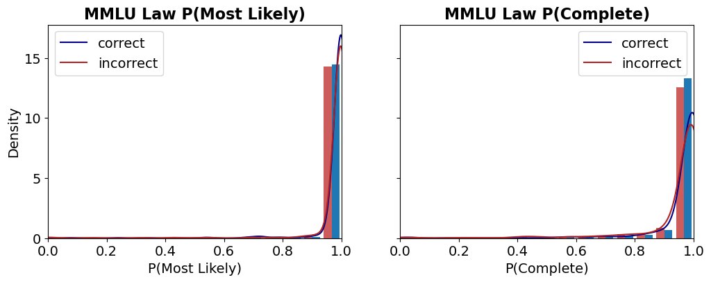
### Visual Description
## Density Plot: MMLU Law Probability Distributions
### Overview
The image displays two side-by-side density plots, each combining a histogram with an overlaid kernel density estimate (KDE) curve. The plots analyze the distribution of probability scores for correct versus incorrect answers on the "MMLU Law" benchmark. The left plot is titled "MMLU Law P(Most Likely)" and the right plot is titled "MMLU Law P(Complete)".
### Components/Axes
* **Titles:**
* Left Plot: "MMLU Law P(Most Likely)"
* Right Plot: "MMLU Law P(Complete)"
* **X-Axes:**
* Left Plot: Label is "P(Most Likely)". Scale ranges from 0.0 to 1.0 with major ticks at 0.0, 0.2, 0.4, 0.6, 0.8, and 1.0.
* Right Plot: Label is "P(Complete)". Scale ranges from 0.0 to 1.0 with major ticks at 0.0, 0.2, 0.4, 0.6, 0.8, and 1.0.
* **Y-Axis (Shared):** Label is "Density". Scale ranges from 0 to 15 with major ticks at 0, 5, 10, and 15.
* **Legends:** Both plots contain an identical legend positioned in the **top-left corner** of the plot area.
* A blue line is labeled "correct".
* A red line is labeled "incorrect".
* **Data Series:** Each plot contains two overlaid series:
1. **Histogram Bars:** Semi-transparent bars showing the binned frequency distribution.
2. **KDE Curves:** Smooth lines showing the estimated probability density function.
### Detailed Analysis
**Left Plot: MMLU Law P(Most Likely)**
* **Trend Verification:** Both the "correct" (blue) and "incorrect" (red) distributions are heavily right-skewed, with the vast majority of density concentrated near a probability of 1.0. The blue "correct" curve shows a sharper, higher peak very close to 1.0 compared to the red "incorrect" curve.
* **Data Points & Distribution:**
* **Correct (Blue):** The histogram bars and KDE curve show an extremely high density peak in the bin from approximately 0.95 to 1.0. The peak density value is approximately 16-17 (slightly above the top y-axis tick of 15). There is negligible density below 0.8.
* **Incorrect (Red):** The distribution also peaks sharply near 1.0, but the peak is slightly lower (density ~14-15) and marginally broader than the "correct" peak. A very small but non-zero density exists in the 0.8 to 0.95 range.
**Right Plot: MMLU Law P(Complete)**
* **Trend Verification:** Both distributions are again right-skewed towards 1.0. However, the separation between the "correct" and "incorrect" distributions is more pronounced here than in the left plot. The "incorrect" distribution has a visibly longer tail extending towards lower probabilities.
* **Data Points & Distribution:**
* **Correct (Blue):** The distribution is tightly clustered near 1.0. The peak density is high, approximately 13-14, located in the 0.95-1.0 bin. Density drops off very sharply below 0.9.
* **Incorrect (Red):** The peak near 1.0 is lower (density ~12) and broader than the "correct" peak. Crucially, there is a noticeable secondary concentration of density (a "shoulder" or minor mode) in the range of approximately 0.8 to 0.9. The tail of the distribution extends further left, with small but visible density bars present down to around 0.6.
### Key Observations
1. **High Confidence Overall:** For both metrics ("Most Likely" and "Complete"), the model assigns very high probabilities (>>0.8) to the vast majority of its answers, regardless of correctness.
2. **Correct Answers Have Higher Confidence:** In both plots, the distribution for correct answers (blue) is more concentrated at the extreme high end (near 1.0) than the distribution for incorrect answers (red).
3. **"Complete" Metric Shows Better Separation:** The distinction between correct and incorrect answer confidence is clearer in the "P(Complete)" plot. Incorrect answers here show a more significant spread into the 0.6-0.9 probability range, whereas in the "P(Most Likely)" plot, even incorrect answers are almost all above 0.9.
4. **Potential Overconfidence:** The fact that incorrect answers still have probabilities peaking near 1.0, especially in the "Most Likely" metric, suggests the model can be highly confident in its wrong answers.
### Interpretation
These plots visualize the calibration and confidence of a model on the MMLU Law benchmark. The data suggests the model is **well-calibrated for correct answers** (high confidence aligns with correctness) but **poorly calibrated for incorrect answers**, exhibiting significant **overconfidence**.
The "P(Most Likely)" metric, which likely measures the probability assigned to the single top-choice answer, shows almost no differentiation in confidence between right and wrong—both are near-certain. This indicates that when the model is wrong, it is often "confidently wrong."
The "P(Complete)" metric, which may represent a probability derived from a more complete answer distribution (e.g., across all options), provides a slightly better signal. Here, incorrect answers show a measurable, though still small, increase in uncertainty (lower probabilities). This implies that analyzing the full answer distribution, rather than just the top choice, might offer a better avenue for detecting model errors or uncertainty.
**In summary:** The model demonstrates high confidence overall, but this confidence is not a reliable indicator of correctness, particularly when looking only at the most likely answer. The "Complete" probability metric offers a marginally better, though still imperfect, separation between correct and incorrect responses.
</details>
Figure 10: Empirical distribution of MMLU explanations when measured via GPT-3.5 probability of being ‘most-likely explanation’ (left) and probability of ‘completely describing’ the question (right). One can see that true (blue) and false (red) answer-conditioned explanations are difficult to distinguish.
### B.5 Sensistivity to Explanation Prompting
Our stable explanation method reweights explanations based on entailment probability, but if the quality of sampled explanations is poor to begin with our resulting distribution will still be inaccurate. Here we will discuss the effect of instructing the LLM to generate explanations before or after an answer (i.e. the order of ‘explanation’ and ‘answer’ in the stability explanation prompt in Figure ˜ 3). We observe in Table ˜ 4 that generating explanations before the answer clearly results in higher quality explanations, as evidenced by improved performance on selective uncertainty and calibration tasks.
| | Pre-Answer Stability (Default) AURC $↑$ | AUROC $↑$ | Post-Answer Stability ECE $↓$ | AURC $↑$ | AUROC $↑$ | ECE $↓$ |
| --- | --- | --- | --- | --- | --- | --- |
| CSQA | 0.901 | 0.779 | 0.123 | 0.866 | 0.731 | 0.201 |
| TruthQA | 0.801 | 0.853 | 0.21 | 0.792 | 0.839 | 0.254 |
| MedQA | 0.784 | 0.798 | 0.169 | 0.743 | 0.743 | 0.251 |
| MMLU Law | 0.642 | 0.736 | 0.259 | 0.629 | 0.706 | 0.289 |
| MMLU Physics | 0.792 | 0.834 | 0.186 | 0.779 | 0.811 | 0.252 |
Table 4: Comparing stability confidence performance using explanations generated before and after an answer for GPT-3.5. One can clearly observe that explanations generated before the answer (i.e. in chain-of-thought fashion) outperform those generated afterwards across all performance metrics.
### B.6 Varying Sample Size
In this section we briefly analyze the effect that the number of sampled explanation has on our confidence metric. In Figure ˜ 11 we observe that selective uncertainty performance (AURC and AUROC) saturates quickly for simpler questions answering tasks such as commonsenseqa. On the other hand MedQA and MMLU Law datasets both demonstrate steady performance gains up to $M=5$ samples per question. Calibration error gradually decreases for all datasets examined.
<details>
<summary>figures/aurc_vs_explanations.png Details</summary>
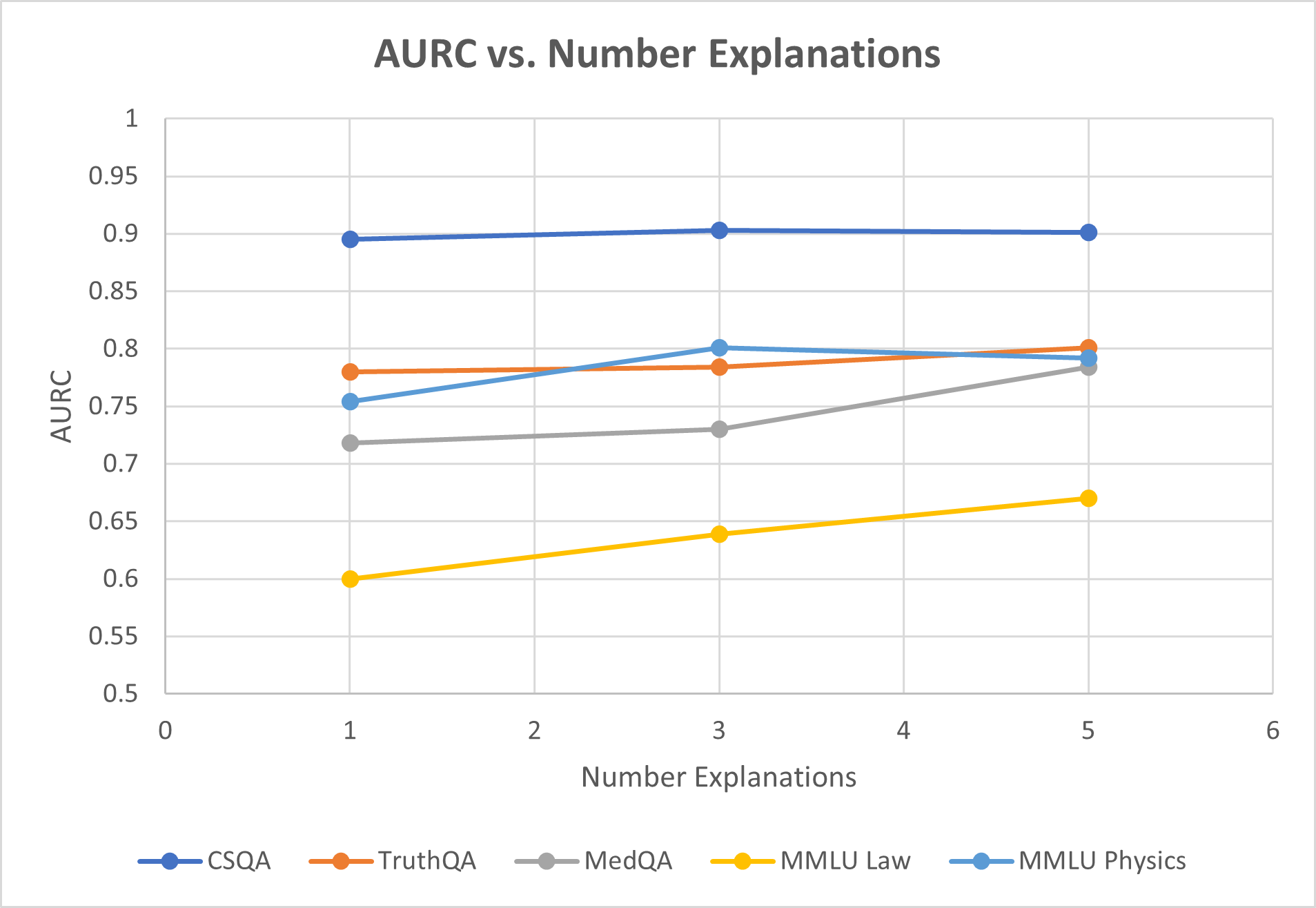
### Visual Description
## Line Chart: AURC vs. Number Explanations
### Overview
This is a line chart titled "AURC vs. Number Explanations." It plots the performance metric "AURC" (likely Area Under the Risk-Coverage curve, a metric for evaluating model confidence or selective prediction) against the "Number Explanations" provided. The chart compares the performance of five different question-answering or reasoning datasets: CSQA, TruthQA, MedQA, MMLU Law, and MMLU Physics.
### Components/Axes
* **Title:** "AURC vs. Number Explanations" (centered at the top).
* **Y-Axis:**
* **Label:** "AURC" (vertical text on the left).
* **Scale:** Linear scale from 0.5 to 1.0, with major gridlines and labels at intervals of 0.05 (0.5, 0.55, 0.6, 0.65, 0.7, 0.75, 0.8, 0.85, 0.9, 0.95, 1).
* **X-Axis:**
* **Label:** "Number Explanations" (horizontal text at the bottom).
* **Scale:** Linear scale from 0 to 6, with major gridlines and labels at integer intervals (0, 1, 2, 3, 4, 5, 6).
* **Legend:** Positioned at the bottom center of the chart. It contains five entries, each with a colored line segment and a circular marker:
* **Dark Blue Line & Marker:** CSQA
* **Orange Line & Marker:** TruthQA
* **Gray Line & Marker:** MedQA
* **Yellow Line & Marker:** MMLU Law
* **Light Blue Line & Marker:** MMLU Physics
* **Grid:** A light gray grid is present for both the x and y axes.
### Detailed Analysis
The chart displays data points at x-values of 1, 3, and 5 for each series. The approximate y-values (AURC) for each data point are as follows:
**1. CSQA (Dark Blue Line):**
* **Trend:** The line is nearly horizontal, showing very stable performance.
* **Data Points:**
* At x=1: y ≈ 0.895
* At x=3: y ≈ 0.90
* At x=5: y ≈ 0.90
**2. TruthQA (Orange Line):**
* **Trend:** The line shows a very slight upward slope, indicating minimal improvement.
* **Data Points:**
* At x=1: y ≈ 0.78
* At x=3: y ≈ 0.785
* At x=5: y ≈ 0.80
**3. MedQA (Gray Line):**
* **Trend:** The line shows a clear upward slope, indicating improvement with more explanations.
* **Data Points:**
* At x=1: y ≈ 0.72
* At x=3: y ≈ 0.73
* At x=5: y ≈ 0.78
**4. MMLU Law (Yellow Line):**
* **Trend:** The line shows a steady, consistent upward slope, indicating the most pronounced improvement among the series.
* **Data Points:**
* At x=1: y ≈ 0.60
* At x=3: y ≈ 0.64
* At x=5: y ≈ 0.67
**5. MMLU Physics (Light Blue Line):**
* **Trend:** The line increases from 1 to 3 explanations, then shows a slight decrease from 3 to 5 explanations.
* **Data Points:**
* At x=1: y ≈ 0.755
* At x=3: y ≈ 0.80
* At x=5: y ≈ 0.79
### Key Observations
1. **Performance Hierarchy:** CSQA consistently achieves the highest AURC (~0.90), followed by TruthQA and MMLU Physics in the 0.75-0.80 range, then MedQA (0.72-0.78), with MMLU Law having the lowest AURC (0.60-0.67).
2. **Impact of Explanations:** For four out of five datasets (all except CSQA), increasing the number of explanations from 1 to 5 is associated with an increase in AURC (improved performance). The magnitude of this improvement varies.
3. **Diminishing Returns/Plateau:** CSQA shows almost no change, suggesting its performance is already near a ceiling with just one explanation. MMLU Physics shows a potential peak at 3 explanations.
4. **Greatest Improver:** MMLU Law shows the largest absolute gain in AURC (~0.07) and the steepest slope, indicating it benefits the most from additional explanations within the tested range.
5. **Crossover:** At 1 explanation, MMLU Physics (light blue) outperforms TruthQA (orange). By 3 explanations, they are nearly equal, and by 5 explanations, TruthQA slightly surpasses MMLU Physics.
### Interpretation
The chart suggests a positive correlation between the number of explanations provided and the AURC performance for most of the evaluated reasoning tasks. This implies that allowing a model to generate or consider multiple explanations can improve its reliability or calibration (as measured by AURC) on these benchmarks.
The varying slopes indicate that the benefit is task-dependent. Tasks like MMLU Law and MedQA, which may involve more complex or specialized reasoning, show a stronger positive response to additional explanations. In contrast, CSQA, which might be a more straightforward commonsense reasoning task, appears robust with minimal explanation. The slight dip for MMLU Physics after 3 explanations could indicate noise, overfitting, or a point where additional explanations introduce confusion rather than clarity for that specific domain.
Overall, the data supports the hypothesis that leveraging multiple explanations is a viable strategy for enhancing the performance of question-answering systems, particularly for tasks where initial performance is lower.
</details>
(a) AURC vs. Number of Explanations for the stable explanations confidence metric.
<details>
<summary>figures/auroc_vs_explanations.png Details</summary>
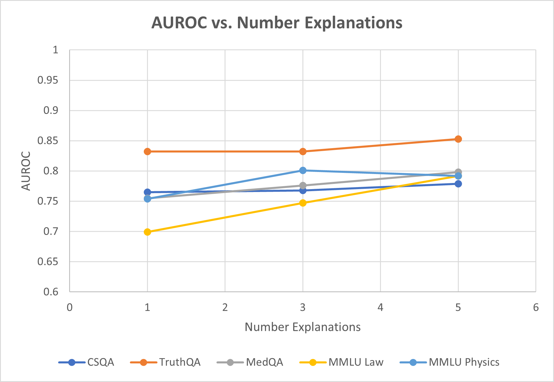
### Visual Description
## Line Chart: AUROC vs. Number Explanations
### Overview
This is a line chart illustrating the relationship between the number of explanations provided (x-axis) and the AUROC (Area Under the Receiver Operating Characteristic curve) performance metric (y-axis) for five different question-answering or reasoning datasets. The chart suggests an analysis of how model performance, as measured by AUROC, changes when the model is given 1, 3, or 5 explanations.
### Components/Axes
* **Chart Title:** "AUROC vs. Number Explanations"
* **Y-Axis:**
* **Label:** "AUROC"
* **Scale:** Linear, ranging from 0.6 to 1.0.
* **Major Gridlines/Ticks:** 0.6, 0.65, 0.7, 0.75, 0.8, 0.85, 0.9, 0.95, 1.0.
* **X-Axis:**
* **Label:** "Number Explanations"
* **Scale:** Linear, with major ticks at integers from 0 to 6.
* **Data Points:** Plotted at x-values of 1, 3, and 5.
* **Legend:** Located at the bottom center of the chart. It defines five data series:
1. **CSQA:** Dark blue line with circular markers.
2. **TruthQA:** Orange line with circular markers.
3. **MedQA:** Gray line with circular markers.
4. **MMLU Law:** Yellow line with circular markers.
5. **MMLU Physics:** Light blue line with circular markers.
### Detailed Analysis
**Data Series Trends and Points:**
1. **TruthQA (Orange Line):**
* **Trend:** Consistently the highest-performing series. Shows a very slight upward trend.
* **Data Points:**
* At 1 Explanation: AUROC ≈ 0.83
* At 3 Explanations: AUROC ≈ 0.83 (appears nearly flat from 1)
* At 5 Explanations: AUROC ≈ 0.85
2. **MMLU Physics (Light Blue Line):**
* **Trend:** Increases from 1 to 3 explanations, then slightly decreases at 5.
* **Data Points:**
* At 1 Explanation: AUROC ≈ 0.755
* At 3 Explanations: AUROC ≈ 0.80
* At 5 Explanations: AUROC ≈ 0.795
3. **MedQA (Gray Line):**
* **Trend:** Shows a steady, moderate upward trend.
* **Data Points:**
* At 1 Explanation: AUROC ≈ 0.755 (overlaps with MMLU Physics start)
* At 3 Explanations: AUROC ≈ 0.775
* At 5 Explanations: AUROC ≈ 0.80
4. **CSQA (Dark Blue Line):**
* **Trend:** Very slight upward trend, nearly flat.
* **Data Points:**
* At 1 Explanation: AUROC ≈ 0.765
* At 3 Explanations: AUROC ≈ 0.77
* At 5 Explanations: AUROC ≈ 0.78
5. **MMLU Law (Yellow Line):**
* **Trend:** Shows the steepest and most consistent upward trend of all series.
* **Data Points:**
* At 1 Explanation: AUROC ≈ 0.70
* At 3 Explanations: AUROC ≈ 0.745
* At 5 Explanations: AUROC ≈ 0.79
### Key Observations
* **Performance Hierarchy:** TruthQA maintains the highest AUROC across all explanation counts. MMLU Law starts as the lowest but shows the greatest improvement, nearly catching up to the middle cluster by 5 explanations.
* **General Trend:** Four out of five datasets (TruthQA, MedQA, CSQA, MMLU Law) show a positive correlation between the number of explanations and AUROC score. The improvement is most dramatic for MMLU Law.
* **Exception:** MMLU Physics is the only series that does not show a net improvement from 3 to 5 explanations, exhibiting a slight decline.
* **Clustering at Start:** At 1 explanation, the datasets form three distinct clusters: high (TruthQA ~0.83), middle (CSQA, MedQA, MMLU Physics ~0.755-0.765), and low (MMLU Law ~0.70).
* **Convergence:** By 5 explanations, the middle cluster (MedQA, MMLU Physics, CSQA) and the rising MMLU Law converge within a narrow band between approximately 0.78 and 0.80 AUROC.
### Interpretation
The data suggests that providing multiple explanations generally enhances a model's discriminative ability (as measured by AUROC) across various knowledge domains. The benefit is not uniform:
* **Domain Sensitivity:** The steep rise for **MMLU Law** indicates that legal reasoning tasks may be particularly sensitive to, and benefit greatly from, additional explanatory context. In contrast, **TruthQA** (likely focused on factual verification) starts with high performance and sees marginal gains, suggesting a ceiling effect or that its core task is less dependent on multiple explanations.
* **The "3-Explanation" Peak for Physics:** The slight dip for **MMLU Physics** from 3 to 5 explanations could indicate noise introduction, overfitting to explanations, or that for physics problems, a moderate amount of explanation is optimal, with more becoming counterproductive. This is an outlier trend worth investigating.
* **Practical Implication:** The chart argues for a tailored approach. For domains like law, investing in generating more explanations yields clear performance returns. For domains like factual QA or physics, the cost-benefit analysis of generating 5 versus 3 explanations needs careful consideration. The overall positive trend supports the hypothesis that rationale-augmented training or inference can improve model reliability.
</details>
(b) AUROC vs. Number of Explanations for the stable explanations confidence metric.
<details>
<summary>figures/ece_vs_explanations.png Details</summary>
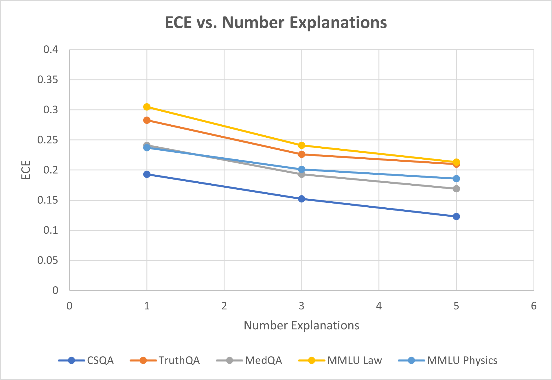
### Visual Description
## Line Chart: ECE vs. Number Explanations
### Overview
The image is a line chart titled "ECE vs. Number Explanations." It plots the Expected Calibration Error (ECE) on the y-axis against the number of explanations on the x-axis for five different question-answering datasets. All five data series show a consistent downward trend, indicating that as the number of explanations increases, the ECE decreases.
### Components/Axes
* **Title:** "ECE vs. Number Explanations" (centered at the top).
* **Y-Axis:**
* **Label:** "ECE" (rotated vertically on the left side).
* **Scale:** Linear scale from 0 to 0.4.
* **Major Gridlines/Ticks:** At intervals of 0.05 (0, 0.05, 0.1, 0.15, 0.2, 0.25, 0.3, 0.35, 0.4).
* **X-Axis:**
* **Label:** "Number Explanations" (centered at the bottom).
* **Scale:** Linear scale from 0 to 6.
* **Major Gridlines/Ticks:** At integer intervals (0, 1, 2, 3, 4, 5, 6).
* **Legend:** Located at the bottom center of the chart. It contains five entries, each with a colored line and marker:
1. **CSQA:** Dark blue line with circular markers.
2. **TruthQA:** Orange line with circular markers.
3. **MedQA:** Gray line with circular markers.
4. **MMLU Law:** Yellow line with circular markers.
5. **MMLU Physics:** Light blue line with circular markers.
* **Plot Area:** Contains five lines connecting data points at x-values of 1, 3, and 5. A light gray grid is present in the background.
### Detailed Analysis
**Trend Verification:** All five lines slope downward from left to right, indicating a negative correlation between the number of explanations and ECE.
**Data Point Extraction (Approximate Values):**
The following table reconstructs the data points. Values are estimated based on the position of the markers relative to the y-axis gridlines.
| Dataset (Legend Color) | x=1 (Number Explanations) | x=3 (Number Explanations) | x=5 (Number Explanations) | Visual Trend Description |
| :--- | :--- | :--- | :--- | :--- |
| **CSQA** (Dark Blue) | ~0.19 | ~0.15 | ~0.12 | Steady, linear decline. Lowest ECE at all points. |
| **TruthQA** (Orange) | ~0.28 | ~0.225 | ~0.21 | Decline, with a slightly shallower slope between x=3 and x=5. |
| **MedQA** (Gray) | ~0.24 | ~0.19 | ~0.17 | Steady, linear decline. |
| **MMLU Law** (Yellow) | ~0.305 | ~0.24 | ~0.215 | Steep initial decline, then a shallower slope. Highest ECE at all points. |
| **MMLU Physics** (Light Blue) | ~0.235 | ~0.20 | ~0.185 | Steady, linear decline. Very close to MedQA at x=1, but diverges slightly higher at x=3 and x=5. |
**Spatial Grounding & Cross-Reference:**
* The legend is positioned at the bottom, centered horizontally.
* At x=1, the vertical order of points from highest to lowest ECE is: MMLU Law (Yellow), TruthQA (Orange), MedQA (Gray), MMLU Physics (Light Blue), CSQA (Dark Blue). This order is confirmed by matching each marker's color to its legend entry.
* At x=5, the order changes slightly: MMLU Law (Yellow) and TruthQA (Orange) are very close at the top, followed by MMLU Physics (Light Blue), MedQA (Gray), and CSQA (Dark Blue) at the bottom.
### Key Observations
1. **Universal Downward Trend:** Every dataset exhibits a reduction in ECE as the number of explanations increases from 1 to 5.
2. **Consistent Hierarchy:** The relative calibration performance (ordering by ECE) of the datasets remains largely consistent across the x-axis, with CSQA consistently having the lowest (best) ECE and MMLU Law consistently having the highest (worst) ECE.
3. **Convergence at Higher Explanations:** The gap between the highest (MMLU Law) and lowest (CSQA) ECE narrows from approximately 0.115 at x=1 to about 0.095 at x=5.
4. **Similar Slopes:** The rates of decline (slopes) for CSQA, MedQA, and MMLU Physics appear very similar and linear. TruthQA and MMLU Law show a slight flattening of the curve between x=3 and x=5.
### Interpretation
The chart demonstrates a clear relationship: providing more explanations (from 1 to 5) is associated with improved model calibration, as measured by a lower Expected Calibration Error (ECE), across all five evaluated QA datasets. This suggests that the process of generating or utilizing multiple explanations helps the model's confidence scores better align with its actual accuracy.
The persistent hierarchy among datasets indicates that inherent characteristics of the tasks or the model's performance on them create a baseline calibration level. For instance, the model appears least calibrated on legal reasoning (MMLU Law) and most calibrated on commonsense reasoning (CSQA), regardless of the number of explanations. The convergence trend hints that increasing explanations may have a slightly greater relative benefit for initially poorly calibrated tasks. This data is crucial for understanding how to improve the reliability of AI systems through explanation-based methods.
</details>
(c) ECE vs. Number of Explanations for the stable explanations confidence metric.
Figure 11: Comparison of stable explanation confidence using different numbers of explanations per question ( $M=\{1,3,5\}$ ). Testing is done on GPT-3.5-Turbo for all five benchmark datasets. One can observe improving but saturating performance for each dataset.
### B.7 Comparison to TTA
Contemporaneously to this manuscript’s submission, another method related to our approach was proposed [28]. The Think-Twice before assure (TTA) method asks for explanations conditioned on different answers, then does a top-k confidence elicitation using these explanations in the prompt. Although similar in the sense that confidence metrics are being generated by conditioning on explanations, their combination of explanations into a single prompt does not match the ensemble of test-time classifiers view that our method takes. The authors have not yet released code or dataset splits, but we have implemented their method by following the written procedure and using the same prompts (see Figure ˜ 12). We found during our implementation on the shared CSQA dataset, the evaluation results for selective uncertainty tasks are slightly below that what the authors report (AURC, AUROC), most likely due to the difference in specific questions used during testing. Nonetheless we report the full results of our implementation in table ˜ 5, and note that this metric does appear to have lower ECE in many cases.
| CSQA | TTA (Our Implementation) AURC $↑$ 0.885 | AUROC $↑$ 0.688 | ECE $↓$ 0.104* | Acc. $↑$ 0.736 |
| --- | --- | --- | --- | --- |
| TruthQA | 0.698 | 0.706 | 0.093* | 0.672* |
| MedQA | 0.641 | 0.581 | 0.207 | 0.505 |
| MMLU Law | 0.574 | 0.657 | 0.148* | 0.456 |
| MMLU Physics | 0.717 | 0.697 | 0.1* | 0.557 |
Table 5: Evaluation for the TTA Confidence metric (Our implementation) on GPT-3.5. Results that outperform our stable explanations metric are marked with an asterisk.
<details>
<summary>figures/tta_prompt.png Details</summary>
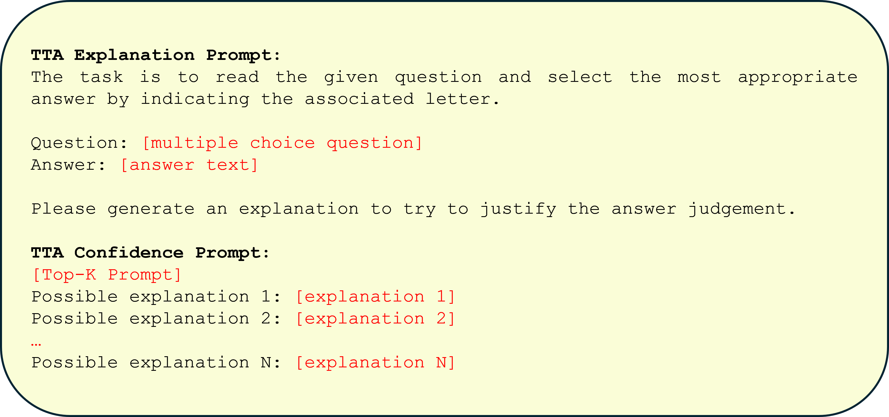
### Visual Description
## Diagram: TTA Prompt Template
### Overview
The image displays a structured text template for a two-stage prompting system, likely for an AI or machine learning evaluation task called "TTA." The template is presented within a rounded rectangular container with a light yellow background and a dark border. It consists of two distinct prompt sections: an "Explanation Prompt" and a "Confidence Prompt," each with specific placeholders for variable content.
### Components
The diagram is a textual layout, not a chart with axes. Its components are:
* **Container:** A rounded rectangle with a pale yellow fill (`#FFFACD` approximate) and a dark blue/black border.
* **Text Blocks:** Left-aligned text in a monospaced font.
* **Color Coding:** Certain placeholder text is rendered in red, while labels and static instructions are in black.
* **Spatial Layout:** The content is organized vertically. The "TTA Explanation Prompt" section occupies the top two-thirds, and the "TTA Confidence Prompt" section occupies the bottom third.
### Content Details
The image contains the following exact textual content, with red text indicated:
**TTA Explanation Prompt:**
The task is to read the given question and select the most appropriate answer by indicating the associated letter.
Question: `[multiple choice question]` *(in red)*
Answer: `[answer text]` *(in red)*
Please generate an explanation to try to justify the answer judgement.
**TTA Confidence Prompt:**
`[Top-K Prompt]` *(in red)*
Possible explanation 1: `[explanation 1]` *(in red)*
Possible explanation 2: `[explanation 2]` *(in red)*
`...`
Possible explanation N: `[explanation N]` *(in red)*
### Key Observations
1. **Two-Stage Process:** The template implies a sequential workflow: first, generating an explanation for a chosen answer, and second, evaluating confidence using multiple potential explanations.
2. **Placeholder System:** Red text consistently marks dynamic fields where specific data (questions, answers, explanations) would be inserted. The ellipsis (`...`) indicates a variable number of explanation slots.
3. **Task Definition:** The first prompt explicitly defines a multiple-choice question-answering task where the output must include both a selected letter and a justifying explanation.
4. **Confidence Mechanism:** The second prompt, labeled "Confidence Prompt," suggests a method for assessing confidence by considering a "Top-K" set of possible explanations, which could be used for ranking or uncertainty estimation.
### Interpretation
This image is not a data visualization but a **specification for a structured AI interaction protocol**. It outlines a method to elicit not just an answer, but also a rationale and a confidence assessment from a model.
* **Purpose:** The template is designed to improve the interpretability and reliability of AI responses. By requiring an explanation, it encourages the model to "show its work." The confidence prompt, which considers multiple explanations, suggests a technique for gauging the certainty of the initial answer—perhaps by checking if alternative, plausible explanations exist.
* **Relationship Between Elements:** The "Explanation Prompt" generates the primary output (answer + justification). The "Confidence Prompt" then uses that output (or variations of it) as input for a secondary evaluation stage. The `[Top-K Prompt]` likely instructs the system on how to generate or retrieve the list of `N` possible explanations.
* **Potential Application:** This structure is common in research on **Chain-of-Thought (CoT) reasoning**, **self-consistency checks**, and **uncertainty quantification** in large language models. It could be used for benchmarking model performance on tasks requiring justification, or in production systems where understanding the model's confidence is critical for decision-making.
* **Notable Design:** The clear separation of the "explanation" and "confidence" stages is a key architectural insight. It modularizes the process of reasoning and self-evaluation, making it easier to analyze and improve each component independently.
</details>
Figure 12: TTA Confidence Prompt
## Appendix C Alternative Perspectives of Stable Explanations
### C.1 Confidence through the Viewpoint of Transductive Inference
Transductive learning selects a classifier at inference-time based on a combination of training and test data [10, 42, 22]. Typically transductive learning involves fine-tuning some classifier parameter $w$ based on an explicit loss objective. However, we claim that using an LLM to generate a sequence of text before an answer (i.e. an explanation) is an alternate way of doing transductive reasoning. First, note that answering a question after an explanation, such as in chain-of-thought prompting [44], effectively changes the decision boundary of the LLM classifier at inference time. Second, consider that when an LLM generates an explanation, it produces concepts related to those in the question. These additional concepts can be thought of as forcing the LLM at inference time to pay more attention to the decision boundary in the area around the test datum. In-context learning literature, which examines LLM performance after manually inserting demonstrations similar to the test question, has already shown a direct connection between transformer context adjustment and classical fine-tuning behavior [9].
To formalize this perspective, let $D^t=\{(x_1,y_1),…,(x_t,y_t)\}$ be a dataset of sequential data up to time $t$ , with $x_i∈ X⊂{ℝ}^M$ and labels $y_i∈ Y⊂\{1,\dots,K\}$ . We denote with $D^t_-=\{(x_1,y_1),\dots,(x_t-1,y_t-1),x_t\}$ the dataset without the last label $y_t$ . We can write our transductive prediction for $x_t$ given data $D^t_-$ including $x_t$ as:
$$
\displaystyle\hat{y}_t=~\underset{w,y}{\rm argmin}~{}\underbrace{\frac{1}{t}\ell(f_w(x_t),y)+\frac{1}{t}∑_i=1^t-1\ell(f_w(x_i),y_i)}_\doteq L(w;(D^t_-,y)). \tag{17}
$$
If $\ell$ is interpreted as a log likelihood, then $L$ can be interpreted as the negative log posterior probability over hypotheses. If we think of optimizing instead over explanations where $f_e(x_t)=φ(x_t,e)$ , then the problem reduces to finding an explanation that strongly supports a single answer without biasing predictions on original test data. The second term in equation ˜ 17 is expensive to compute at inference time, but if some approximation of this training loss existed it would make optimization tractable. We hypothesize that if the explanation under consideration is plausible and faithful to the question (as determined using the same LLM), it should not reduce the accuracy of previous decisions too much. Therefore we can avoid having to optimize over all previous questions and instead optimize over whatever faithfulness measure $g_φ(e)$ we define:
$$
\displaystyle\hat{y}_t=~\underset{e,y}{\rm argmin}~{}\ell(φ(x_t,e),y)+λ g_φ(e) \tag{18}
$$
This looks exactly like the typical transductive setting but with a more easily computable ‘transductive prior’.
### C.2 Confidence throught the Viewpoint of Solomonoff Induction
While transductive inference typically finds single test-time classifier, our method looks for a distribution of likely classifiers. In this sense, our method can be seen as a special case of Solomonoff induction [25]. Solomonoff induction considers how well data-generating programs, $H$ , (i.e. a binary string run on a Turing machine) explain the test data, $D$
$$
\displaystyle P(H|D)=\frac{P(D|H)P(H)}{P(D|H)P(H)+∑_A≠ HP(D|A)P(A)}, \tag{19}
$$
where $A$ are alternative programs. Solomonoff induction formalizes the principle of Occam’s razor by choosing a universal prior $P(H)$ that gives a higher probability to shorter-length programs. Then to predict new data $D^\prime$ given previous observations, one simply computes
$$
\displaystyle P(D^\prime|D)=E_H[P(D^\prime|H,D)]=∑_HP(D^\prime|H,D)P(H|D). \tag{20}
$$
While these Bayesian equations seem simple, Solomonoff’s induction is provably uncomputable. However, our method can be interpreted as restricting our hypothesis class from the set of all computable programs $H$ to the set of all LLM-interpretable programs $e$ . Instead of a prior on program length, we can use the LLM’s prior likelihood of valid sequences in the language $p_φ(e)$ . This restriction makes our calculations more tractable, as we can easily approximate expectations over our hypothesis class by sampling explanations from the LLM.
### C.3 Confidence through the Viewpoint of Stability
Another recent line of work has been analyzing LLMs through the lens of stochastic dynamical models [37]. Through the perspective of stability analysis one could interpret our method’s preference for explanations convening to a single answer as searching for fixed points of a specific LLM system. This LLM dynamical system consists of two alternating steps, first generating an explanation conditioned on one of the answers ( $e←φ(q,a)$ ) then generating a new answer based on this explanation ( $a^\prime←φ(q,e)$ ). Intuitively this system mirrors how a human expert may think about a question by considering alternative conclusions one could draw given beliefs about the world. An answer with only a single plausible explanation that strongly supports that same answer (i.e. decision distribution collapses to a singleton) forms a stable cycle in this system.