2406.03816

# ReST-MCTS∗: LLM Self-Training via Process Reward Guided Tree Search [backgroundcolor=yellow!10,outerlinecolor=black,innertopmargin = littopskip = ntheorem = false,roundcorner=2pt] framedtheoremTheorem [backgroundcolor=gray!10,outerlinecolor=black,innertopmargin = littopskip = ntheorem = false,roundcorner=2pt] assumptionAssumption [backgroundcolor=gray!8,outerlinecolor=black,innertopmargin = littopskip = ntheorem = false,roundcorner=2pt] observationObservation ## Abstract Recent methodologies in LLM self-training mostly rely on LLM generating responses and filtering those with correct output answers as training data. This approach often yields a low-quality fine-tuning training set (e.g., incorrect plans or intermediate reasoning). In this paper, we develop a reinforced self-training approach, called ReST-MCTS ∗, based on integrating process reward guidance with tree search MCTS ∗ for collecting higher-quality reasoning traces as well as per-step value to train policy and reward models. ReST-MCTS ∗ circumvents the per-step manual annotation typically used to train process rewards by tree-search-based reinforcement learning: Given oracle final correct answers, ReST-MCTS ∗ is able to infer the correct process rewards by estimating the probability this step can help lead to the correct answer. These inferred rewards serve dual purposes: they act as value targets for further refining the process reward model and also facilitate the selection of high-quality traces for policy model self-training. We first show that the tree-search policy in ReST-MCTS ∗ achieves higher accuracy compared with prior LLM reasoning baselines such as Best-of-N and Tree-of-Thought, within the same search budget. We then show that by using traces searched by this tree-search policy as training data, we can continuously enhance the three language models for multiple iterations, and outperform other self-training algorithms such as ReST ${}^EM$ and Self-Rewarding LM. We release all code at https://github.com/THUDM/ReST-MCTS. footnotetext: Equal contribution. footnotetext: Work done while DZ visited at Caltech. ### 1 Introduction Large Language Models (LLMs) are mostly trained on human-generated data. But as we approach the point where most available high-quality human-produced text on the web has been crawled and used for LLM training [1], the research focus has shifted towards using LLM-generated content to conduct self-training [2; 3; 4; 5; 6; 7]. Similar to most Reinforcement Learning (RL) problems, LLM self-training requires a reward signal. Most existing reinforced self-improvement approaches (e.g., STaR [4], RFT [5], ReST ${}^EM$ [6], V-STaR [7]) assume to have access to a ground-truth reward model (labels from supervised dataset, or a pre-trained reward model). These approaches use an LLM to generate multiple samples for each question, and assume the one that leads to high reward (correct solution) is the high-quality sample, and later train on these samples (hence self-training). Such procedures can be effective in improving LLM performance, in some cases solving reasoning tasks that the base LLM cannot otherwise solve [8; 9; 10]. Table 1: Key differences between existing self-improvement methods and our approach. Train refers to whether to train a reward model. | Method | Reasoning Policy | Reward Guidance | | | --- | --- | --- | --- | | Method | Value Label | Train | | | STaR [4] | CoT+Reflexion | Final outcome reward annotated by ground-truth answer | ✗ | | ReST ${}^EM$ [6] / RFT [5] / RPO [11] | CoT | ✗ | | | Verify Step-by-Step [1] | Best-of-N | Per-step process reward annotated by human | ✓ | | MATH-SHEPHERD [12] / pDPO [13] | Best-of-N | Per-step process reward inferred from random rollout | ✓ | | TS-LLM [14] | MCTS | Per-step process reward inferred from TD- $λ$ [15] | ✓ | | V-STaR [7] | CoT | Final outcome reward generated by multi-iteration LLMs | ✓ | | Self-Rewarding [16] | CoT | Final outcome reward generated and judged by LLMs | ✗ | | ReST-MCTS ∗ (Ours) | MCTS ∗ | Per-step process reward inferred from tree search (MCTS ∗) | Multi-Iter | However, a key limitation of the above procedure is that even if a reasoning trace results in a correct solution, it does not necessarily imply that the entire trace is accurate. LLMs often generate wrong or useless intermediate reasoning steps, while still finding the correct solution by chance [17]. Consequently, a self-training dataset can often contain many false positives — intermediate reasoning traces or plans are incorrect, but the final output is correct — which limits the final performance of LLM fine-tuning for complex reasoning tasks [18; 19]. One way to tackle this issue is to use a value function or reward model to verify reasoning traces for correctness (which then serves as a learning signal for self-training) [1; 12]. However, training a reliable reward model to verify every step in a reasoning trace generally depends on dense human-generated annotations (per reasoning step) [1], which does not scale well. Our research aims to address this gap by developing a novel approach that automates the acquisition of reliable reasoning traces while effectively utilizing reward signals for verification purposes. Our key research question is: How can we automatically acquire high-quality reasoning traces and effectively process reward signals for verification and LLM self-training? In this paper, we propose ReST-MCTS ∗, a framework for training LLMs using model-based RL training. Our proposed approach utilizes a modified Monte Carlo Tree Search (MCTS) algorithm as the reasoning policy, denoted MCTS ∗, guided by a trained per-step process reward (value) model. A key aspect of our method is being able to automatically generate per-step labels for training per-step reward models, by performing a sufficient number of rollouts. This labeling process effectively filters out the subset of samples with the highest quality, without requiring additional human intervention. Table 1 summarizes the key distinctions between our approach and previous approaches. We validate experimentally that ReST-MCTS ∗ outperforms prior work in discovering good reasoning traces, such as Self-Consistency (SC) and Best-of-N (BoN) under the same search budget on the SciBench [20] and MATH [21] benchmarks, which consequently leads to improved self-training. To summarize, our contributions are: - We propose ReST-MCTS ∗, a self-training approach that generates process rewards searched by MCTS ∗. A key step is to automatically annotate the process reward of each intermediate node via sufficient times of rollouts, using MCTS ∗. We validate multiple reasoning benchmarks and find that ReST-MCTS ∗ outperforms existing self-training approaches (e.g., ReST ${}^EM$ and Self-Rewarding) as shown in Table 2 and reasoning policies (e.g., CoT and ToT) as shown in Table 4. - The reward generator in ReST-MCTS ∗ leads to a higher-quality process reward model compared to previous process reward generation techniques, e.g., MATH-SHEPHERD, as shown in Table 3. 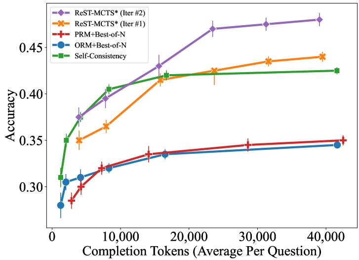- Given the same search budget, the search algorithm (MCTS ∗) in ReST-MCTS ∗ achieves higher accuracy than Self-Consistency and Best-of-N, as shown in Figure 2. ### 2 Background on Reasoning & Self-Training We follow the standard setup in LLM-based reasoning. We start with a policy, denoted by $π$ , that is instantiated using a base LLM. Given an input problem $Q$ , in the simplest case, $π$ can generate an output sequence, or trace, of reasoning steps $(s_1,s_2,⋯,s_K)∼π(·|Q)$ by autoregressively predicting the next token. For simplicity, we assume a reasoning step comprises a single sentence (which itself comprises multiple tokens). We also assume the last output $s_K$ is the final step. LLMs can also be prompted or conditioned to bias the generation along certain traces. For a prompt $c$ , we can write the policy as $π(·|Q,c)$ . This idea was most famously used in chain-of-thought (CoT) [22]. Self-Consistency (SC). Self-Consistency [23] samples multiple reasoning traces from $π$ and chooses the final answer that appears most frequently. Tree-Search & Value Function. Another idea is to use tree-structured reasoning traces [24; 14], that branch from intermediate reasoning steps. One key issue in using a so-called tree-search reasoning algorithm is the need to have a value function to guide the otherwise combinatorially large search process [14]. Two common value functions include Outcome Reward Models (ORMs) [25], which are trained only on the correctness of the final answer, and Process Reward Models (PRMs) [1], which are trained on the correctness of each reasoning step. We assume $r_s_{k}$ is the PRM’s output sigmoid score at $k$ -th step. Our ReST-MCTS ∗ approach uses tree-search to automatically learn a good PRM. Best-of-N. As an alternative to Self-Consistency, one can also use a learned value function (PRM or ORM) to select the reasoning trace with the highest value [1]. Self-Training. At a high level, there are two steps to self-training [6; 12]. The first step is generation, where we sample multiple reasoning traces using $π$ (in our case, tree-structured traces). The second step is improvement, where a learning signal is constructed on the reasoning traces, which is then used to fine-tune $π$ . The process can repeat for multiple iterations. Limitation of Prior Works. The main challenge in doing reliable self-training is the construction of a useful learning signal. Ideally, one would want a dense learning signal on the correctness of every intermediate reasoning step, which is given by a PRM. Otherwise, with sparse learning signals, one suffers from a credit assignment similar to that in reinforcement learning. Historically, the main challenge with learning a PRM is the lack of supervised annotations per reasoning step. This is the principal challenge that our ReST-MCTS ∗ approach seeks to overcome. We describe detailed preliminaries in Appendix A. 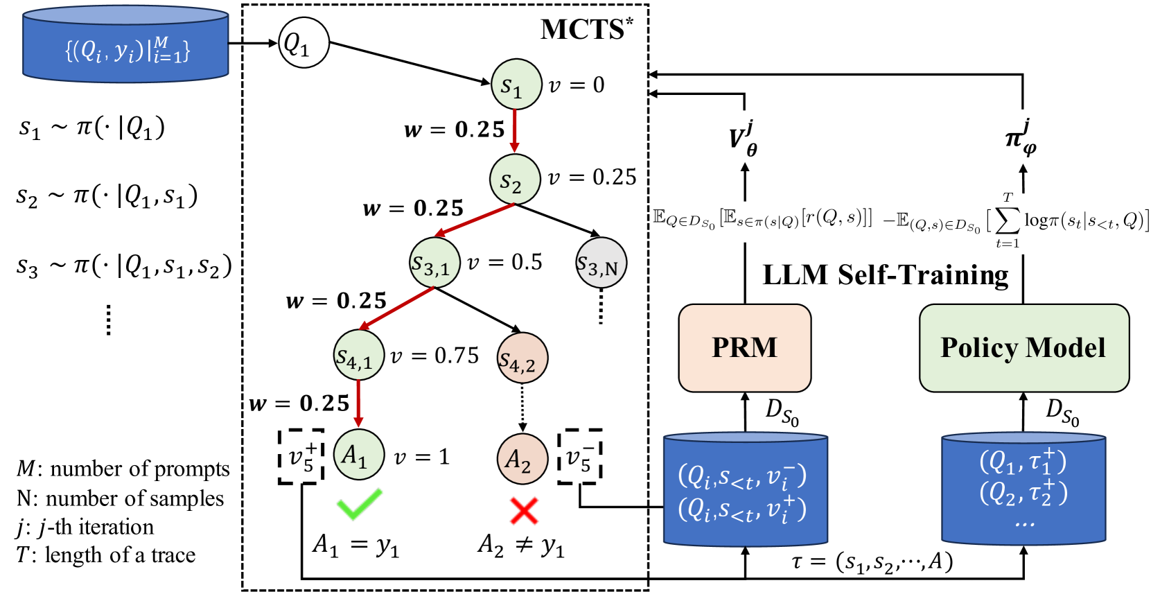### 3 The ReST-MCTS ∗ Method Our approach, ReST-MCTS ∗, is outlined in Figure 1 and developed using four main components. - MCTS ∗ which performs a tree search with sufficient rollout time under the guidance of the PRM. - Process Reward Model (PRM) which evaluates any partial solution’s quality and guides MCTS ∗. - Policy Model which generates multiple intermediate reasoning steps for each question. - LLM Self-Training, which uses MCTS ∗ to collect reasoning traces, trains policy model on positive samples, and trains process reward model on all generated traces. <details> <summary>x1.png Details</summary>  ### Visual Description ## Diagram: MCTS*-Based LLM Self-Training Framework ### Overview This image is a technical diagram illustrating a machine learning training pipeline that combines Monte Carlo Tree Search (MCTS*) with Large Language Model (LLM) self-training. The system uses a dataset of prompts and responses to generate reasoning traces via MCTS, evaluates them with a Process Reward Model (PRM), and updates a Policy Model. The diagram is divided into three main regions: a left-side data input and sampling section, a central MCTS* tree search process, and a right-side LLM self-training loop. ### Components/Axes **Left Region (Data Input & Sampling):** - **Top-left blue cylinder:** Labeled `{(Q_i, y_i)}|_{i=1}^{M}`. This represents a dataset of `M` prompt-response pairs. - **Sampling equations below the cylinder:** - `s_1 ~ π(· | Q_1)` - `s_2 ~ π(· | Q_1, s_1)` - `s_3 ~ π(· | Q_1, s_1, s_2)` - A vertical ellipsis (`⋮`) indicates continuation. - **Legend (bottom-left):** - `M`: number of prompts - `N`: number of samples - `j`: j-th iteration - `T`: length of a trace **Central Region (MCTS* Tree Search):** - Enclosed in a dashed box labeled **MCTS*** at the top. - **Tree Structure:** - Root node: `Q_1` (circle). - First level: Node `s_1` with value `v = 0`. - A red arrow points from `s_1` to `s_2` with weight `w = 0.25`. - Node `s_2` has value `v = 0.25`. - From `s_2`, a red arrow points to node `s_{3,1}` with `w = 0.25` and `v = 0.5`. Another branch (black arrow) points to node `s_{3,N}`. - From `s_{3,1}`, a red arrow points to node `s_{4,1}` with `w = 0.25` and `v = 0.75`. Another branch points to node `s_{4,2}`. - From `s_{4,1}`, a red arrow points to terminal node `A_1` with `w = 0.25` and `v = 1`. A green checkmark (✓) is below it, with the label `A_1 = y_1`. - From `s_{4,2}`, a dotted line points to terminal node `A_2`. A red cross (✗) is below it, with the label `A_2 ≠ y_1`. - **Value Feedback Boxes:** - A dashed box labeled `v_5^+` is connected to `A_1`. - A dashed box labeled `v_5^-` is connected to `A_2`. **Right Region (LLM Self-Training):** - Labeled **LLM Self-Training** at the top. - **Two main model blocks:** 1. **PRM** (peach-colored rectangle): Process Reward Model. 2. **Policy Model** (light green rectangle). - **Equations above the models:** - Above PRM: `E_{Q∈D_{S_0}}[E_{s∈π(s|Q)}[r(Q, s)]]` - Above Policy Model: `-E_{(Q,s)∈D_{S_0}}[∑_{t=1}^{T} log π(s_t | s_{<t}, Q)]` - **Data Stores (blue cylinders):** - **Left cylinder (feeds PRM):** Labeled `D_{S_0}`. Contains tuples: `(Q_i, s_{<t}, v_i^-)` and `(Q_i, s_{<t}, v_i^+)`. - **Right cylinder (feeds Policy Model):** Labeled `D_{S_0}`. Contains tuples: `(Q_1, τ_1^+)`, `(Q_2, τ_2^+)`, and a vertical ellipsis (`...`). - **Trace Input:** A trace `τ = (s_1, s_2, ..., A)` is shown at the bottom, with arrows pointing into both blue data store cylinders. - **Model Outputs:** - An arrow from PRM points upward to `V_θ^j`. - An arrow from Policy Model points upward to `π_φ^j`. - Both `V_θ^j` and `π_φ^j` have arrows pointing back into the MCTS* box, indicating they are used in the search process. ### Detailed Analysis **Flow and Relationships:** 1. **Initialization:** The process starts with a dataset of prompts (`Q_i`) and correct answers (`y_i`). 2. **MCTS* Exploration:** For a given prompt `Q_1`, the MCTS* algorithm explores a tree of reasoning steps (`s_1, s_2, ...`). Each step is sampled from a policy `π`. The tree assigns a value `v` (increasing from 0 to 1 along the successful path) and a weight `w` (consistently 0.25 on the highlighted red path). 3. **Outcome Evaluation:** The search terminates at actions `A_1` (correct, matches `y_1`) and `A_2` (incorrect). These generate positive (`v_5^+`) and negative (`v_5^-`) reward signals. 4. **Data Collection:** The generated traces (`τ`), states (`s_{<t}`), and reward signals are stored in the `D_{S_0}` datasets. 5. **Model Training:** - The **PRM** is trained on state-reward pairs to learn a value function `V_θ^j`. - The **Policy Model** is trained on successful traces (`τ^+`) to improve its action selection, resulting in policy `π_φ^j`. 6. **Feedback Loop:** The updated value function (`V_θ^j`) and policy (`π_φ^j`) are fed back into the MCTS* process for the next iteration (`j`), creating a self-improving loop. ### Key Observations - The **red arrows** in the MCTS* tree highlight a specific, high-value path from the root to the correct answer `A_1`. - The **weight `w`** is constant at 0.25 along this highlighted path, suggesting a uniform sampling or exploration strategy within this branch. - The **value `v`** increases monotonically (0 → 0.25 → 0.5 → 0.75 → 1) along the successful path, indicating the model's growing confidence or the reward accumulation. - The diagram explicitly separates **process-level rewards** (handled by PRM, which evaluates intermediate states `s`) from **outcome-level rewards** (the final correct/incorrect check). - The **Policy Model** is trained only on positive traces (`τ^+`), while the **PRM** is trained on both positive and negative state-reward pairs. ### Interpretation This diagram depicts a sophisticated **reinforcement learning from AI feedback (RLAIF)** or **self-play** framework for reasoning. The core idea is to use a search algorithm (MCTS*) to generate diverse reasoning paths for a given problem. These paths are then automatically evaluated—both at intermediate steps (by the PRM) and at the final outcome—to create a training signal without human labeling. The system demonstrates a **closed-loop improvement cycle**: the model's own outputs (traces) and their automated evaluation are used to train better versions of its components (value function and policy), which in turn guide more effective future search. This approach aims to enhance the LLM's ability to perform multi-step reasoning, exploration, and self-correction. The use of MCTS* suggests an emphasis on balancing exploration of new reasoning paths with exploitation of known good ones. The clear separation of the PRM (which learns *what* is a good step) and the Policy Model (which learns *how* to generate such steps) is a key architectural insight for scalable self-improvement. </details> Figure 1: The left part presents the process of inferring process rewards and how we conduct process reward guide tree-search. The right part denotes the self-training of both the process reward model and the policy model. #### 3.1 Search-based Reasoning Policy for LLM Value $v_k$ for a Partial Solution. The value (process) reward $v_k$ of the partial solution $p_k=[s_1,s_2,⋯,s_k]$ should satisfy the following basic qualities: - Limited range: $v_k$ is constrained within a specific range. This restriction ensures that the values of $v_k$ are bounded and do not exceed a certain limit. - Reflecting probability of correctness: $v_k$ reflects the probability that a partial solution is a complete and correct answer. Higher values of $v_k$ indicate better quality or a higher likelihood of being closer to a correct answer. - Reflecting correctness and contribution of solution steps: $v_k$ incorporates both the correctness and contribution of each solution step. When starting from a partial solution, a correct next step should result in a higher $v_k$ compared to false ones. Additionally, a step that makes more correct deductions toward the final answer should lead to a higher $v_k$ value. This property ensures that $v_k$ captures the incremental progress made towards the correct solution and rewards steps that contribute to the overall correctness of the solution. Reasoning Distance $m_k$ for a Partial Solution. To estimate the progress of a solution step, we define the reasoning distance $m_k$ of $p_k$ as the minimum reasoning steps a policy model requires to reach the correct answer, starting from $p_k$ . Reasoning distance reflects the progress made as well as the difficulty for a policy to figure out a correct answer based on current steps, thus it can be further used to evaluate the quality of $p_k$ . However, we point out that $m_k$ can not be directly calculated. It is more like a hidden variable that can be estimated by performing simulations or trace sampling starting from $p_k$ and finding the actual minimum steps used to discover the correct answer. Weighted Reward $w_s_{k}$ for a Single Step. Based on the desired qualities for evaluating partial solutions, we introduce the concept of a weighted reward to reflect the quality of the current step $s_k$ , denoted as $w_s_{k}$ . Based on the common PRM reward $r_s_{k}$ , $w_s_{k}$ further incorporates the reasoning distance $m_k$ as a weight factor, reflecting the incremental progress $s_k$ makes. Representations for Quality Value and Weighted Reward. To determine the quality value $v_k$ of a partial solution at step $k$ , we incorporate the previous quality value and the weighted reward of the current step. By considering the previous quality value, we account for the cumulative progress and correctness achieved up to the preceding step. Therefore, the $v_k$ can be iteratively updated as: $$ \displaystylev_k=≤ft\{\begin{array}[]{cc}0,&k=0\\ max(v_k-1+w_s_{k},0),&else\end{array}\right. \tag{3} $$ The weighted reward $w_s_{k}$ of the current step provides a measure of the quality and contribution of that specific step towards the overall solution. Based on $m_k$ (where $m_k=K-k$ and $K$ is the total number of reasoning steps of a solution $s$ ), previous quality value $v_k-1$ , and $r_s_{k}$ in MATH-SHEPHERD [12], we can update the definition of the weighted reward $w_s_{k}$ iteratively as follows: $$ \displaystylew_s_{k}=\frac{1-v_k-1}{m_k+1}(1-2r_s_{k}), k=1,2,⋯ \tag{4} $$ As $k$ increases, $m_k$ decreases, indicating that fewer reasoning steps are needed to reach the correct answer. This leads to a higher weight placed on the weighted reward of the current step. We can also derive that $w_s_{k}$ and $v_k$ satisfy the expected boundedness shown in the theorem below. **Theorem 1 (Boundedness ofwsksubscript𝑤subscript𝑠𝑘w_{s_{k}}italic_w start_POSTSUBSCRIPT italic_s start_POSTSUBSCRIPT italic_k end_POSTSUBSCRIPT end_POSTSUBSCRIPTandvksubscript𝑣𝑘v_{k}italic_v start_POSTSUBSCRIPT italic_k end_POSTSUBSCRIPT)** *If $r_s_{k}$ is a sigmoid score ranged between $[0,1]$ , then $w_s_{k}$ and $v_k$ defined as above satisfy following boundedness: $w_s_{k}≤ 1-v_k-1$ , $v_k∈[0,1]$ .* Derivation. Please refer to the detailed derivation in Appendix B.1. Therefore, we can conclude that $w_s_{k}$ and $v_k$ has following properties that match our expectations: If a reasoning route starting from $p_k$ requires more steps to get to the correct answer, then the single-step weighted reward $w_s_{k}$ is lower. $w_s_{k}$ decreases as the PRM’s predicted sigmoid score $r_s_{k}$ rises. Thus, $w_s_{k}$ has a positive correlation with the PRM’s prediction of a step’s correctness. $v_k→ 1\iff r_s_{k}→ 0, m_k=0$ , i.e. $v_k$ converges to upper bound $1$ only when $s_k$ reaches the correct answer. Based on the features of $v_k$ and $w_s_{k}$ , we can directly predict the quality value of partial solutions and guide search once we have a precise PRM and accurate prediction of $m_k$ . In our approach, instead of separately training models to predict $r_s_{k}$ and $m_k$ , we simply train a process reward model $V_θ$ to predict $v_k$ , serving as a variant of common PRM. With reward incorporated in the calculation of $v_k$ , there is no need to separately train a reward model, saving considerable effort for answer selection. Process Reward Model Guided Tree Search MCTS ∗. Tree search methods like [24] and [26] require a value function and outcome reward model $r_φ$ to prune branches, evaluate final solutions and backup value. However, using ORM to evaluate final solutions and backpropagate means every search trace must be completely generated, which is costly and inefficient. Recent work [14] suggests using a learned LLM value function in MCTS so the backup process can happen in the intermediate step, without the need for complete generations. Their work greatly improves search efficiency but still relies on an ORM to select the final answer. Drawing inspiration from these works, we further propose a new variant of MCTS, namely MCTS ∗, which uses quality value $v_k$ as a value target for a trained LLM-based process reward model and guidance for MCTS as well. Given the above properties, we can directly use the process reward model $V_θ$ to evaluate the quality of any partial solution, select, and backpropagate in intermediate nodes. Aside from the use of quality value, we also incorporate a special Monte Carlo rollout method and self-critic mechanism to enhance efficiency and precision, which are explained detailedly in Appendix C.1. We express MCTS ∗ as an algorithm that comprises four main stages in each iteration, namely node selection, thought expansion, greedy MC rollout, and value backpropagation. Similar to common MCTS settings, the algorithm runs on a search tree $T_q$ for each single science reasoning question $q$ . Every tree node $C$ represents a series of thoughts or steps, where a partial solution $p_C$ , number of visits $n_C$ , and corresponding quality value $v_C$ are recorded. For simplicity, we denote each node as a tuple $C=(p_C,n_C,v_C)$ . An overall pseudo-code for MCTS ∗ is presented in Algorithm 2. #### 3.2 Self-Training Pipeline As shown in Figure 1, based on the proposed tree search algorithm MCTS ∗, we perform self-improvement on the reasoning policy and process reward model. After initialization of the policy $π$ and process reward model $V_θ$ , we iteratively employ them and utilize the search tree $T_q$ generated in the process to generate high-quality solutions for specific science or math questions and conduct a self-improvement process, called ReST-MCTS ∗. Our work draws inspiration from the MuZero [20] framework and applies it to the training of LLMs which we term “MuZero-style learning of LLMs”. Instruction Generation. In this stage, initialization starts from an original dataset $D_0$ for the training process reward model $V_θ$ . $\bullet$ Collect process reward for process reward model. The extraction of new value data is relatively more complex, we derive the target quality value of partial solutions of every tree node near a correct reasoning path on the pruned search tree $T_q^{^\prime}$ . We first calculate $m_k$ for every tree node $C$ that is on at least one correct reasoning trace (including the root) according to its minimum reasoning steps required to get to a correct answer in $T_q^{^\prime}$ . Then, we use the hard estimation in Eq. (13) in [12] to calculate $r_s_{k}$ , i.e. $r_s_{k}=1-r_s_{k}^HE$ , which means a reasoning step is considered correct if it can reach a correct answer in $T_q^{^\prime}$ . Using $m_k$ and $r_s_{k}$ , we are able to derive the value of the partial solution of every node on or near one correct reasoning trace. For each node $C$ (with partial solution $p_C=[s_1,s_2,⋯,s_k-1]$ ) on at least one correct trace and a relevant forward step $s_k$ , we can derive the value $v_k$ using Eq. (3) and weighted reward $w_k$ using Eq. (4), with $m_k$ set to the same as $m_k-1$ if $r_s_{k}^HE=0$ in Eq. (13). A concrete and detailed example of this inferring process is shown in Figure 3. We update all these rewards and values starting from the root and collect all $(Q,p,v)$ pairs to form $D_V_{i}$ in $i$ -th iteration, which is used for training a process reward model in the next iteration. $\bullet$ Collect reasoning traces for policy model. As shown in Figure 4, the search process produces a search tree $T_q$ , consisting of multiple reasoning traces. We first prune all the unfinished branches (branches that do not reach a final answer). Then we verify other traces’ final answers acquired in the tree search according to their correctness through simple string matching or LLM judging and select the correct solutions. These verified reasoning traces, as $D_G_{i(A_j=a^*)|_j=1^N}$ (where $N$ is the number of sampling solutions, $A_j$ is the $j$ -th solution, and $a^*$ is the final correct answer) in $i$ -th iteration, are then used for extracting new training data for policy self-improvement. This process is followed by Eq. (15) ( $i≥ 1$ ) to execute the policy self-training. Mutual Self-training for Process Reward Model and Policy Model. Compared to previous work like ReST ${}^EM$ [6], which only concerns self-training for the policy and demonstrates that the policy can improve by iteratively generating new traces and learning from the high-reward ones generated by itself, our work simultaneously improves the process reward model and policy model self-training. With the process reward model’s training set $D_V_0$ initialized and new problem set $D_G$ given, we can start the iterative self-training process upon $V_θ$ and $π$ . We use $π$ to perform MCTS ∗ and generate solutions for $D_G$ , with implement details illustrated in Section 3.1. In the $i$ -th ( $i=1,2,⋯)$ iteration, we train $V_θ$ with $D_V_{i-1}$ to obtain $V_i$ and train policy model $π_S_{i-1}$ on $D_G_{i}$ to generate new generator $π_S_{i}$ . At the same time, $D_G_{i}$ drives the update of $V_i$ to $V_i+1$ . We present iterative self-training that the process reward model and policy model complement each other in Algorithm 1. 0: base LLM $π$ , original dataset for policy model $D_S_0$ , original dataset for value model $D_0$ , new problem set $D_G$ , number of solutions $N$ , $j$ -th solution $A_j$ , correct solution $a^*$ , value model $V_θ$ , weighted value function $w$ , quality value function $v$ , number of iterations $T$ . 1: $π_S_0←$ SFT( $π,D_S_0$ ) // fine-tune generator 2: $D_V_0←$ generate $\_$ value $\_$ data( $D_0,w,v$ ) // initialize train set for value model 3: $V_0←$ train $\_$ value $\_$ model( $V_θ,D_V_0$ ) // initialize value model 4: for $i=1$ to $T$ do 5: $D_G_{i}←$ generate $\_$ policy $\_$ data( $π_S_{i-1}$ , $V_i-1$ guided MCTS ∗, $D_G$ , $N$ ) // generate synthetic data for policy model 6: for $j=1$ to $N$ do 7: $D_G_{i(A_j=a^*)}←$ label $\_$ correctness( $D_G_{i}$ ) // match and select correct solutions 8: end for 9: $π_S_{i}←$ SFT( $π_S_{i-1},D_G_{i(A_j=a^*)|_j=1^N}$ ) // self-training policy model 10: $D_V_{i}←$ extract $\_$ value $\_$ data( $D_G_{i}$ ) // collect process reward and extract value data 11: $V_i←$ train $\_$ value $\_$ model( $V_i-1,D_V_{i}$ ) // self-training value model 12: end for 12: $π_S_{T},V_T$ Algorithm 1 Mutual self-training ReST-MCTS ∗ for value model and policy model. ### 4 Experiments We validate ReST-MCTS ∗ from three perspectives: $\bullet$ Self-Training approaches which use generated samples and evaluated for multiple iterations, such as ReST ${}^EM$ and Self-Rewarding, on in-distribution and out-of-distribution benchmarks under three LLM backbones, as shown in Table 2. ReST-MCTS ∗ outperforms existing approaches in each iteration and continuously self-improves with the data it generates. $\bullet$ Process reward models which are compared with the state-of-the-art techniques, such as MATH-SHEPHERD (MS) and SC + MS on GSM8K and MATH500, as shown in Table 3. Results indicate that the ReST-MCTS ∗ learns a good PRM and our reward model implements higher accuracy. $\bullet$ Tree-Search policy which are compared on college-level scientific reasoning benchmark under three LLMs, such as CoT and ToT, as shown in Table 4. We also evaluated under the same search budget on MATH and SciBench, such as SC and Best-of-N, as shown in Figure 2. Results show the ReST-MCTS ∗ significantly outperforms other baselines despite insufficient budget. #### 4.1 Initialization of Value Model To obtain accurate feedback from the environment, we build the value model’s initial train set $D_V_0$ from a set of selected science or math questions $D_0$ using process reward (value) inference, with no human labeling process required. Then, we finetune the ChatGLM3-6B [27; 28] and Mistral-7B [29] model on this dataset, respectively, obtaining initial value models that, as variants of PRM, guide the LLM tree search for higher-quality solutions upon both math and science questions. Fine-grained dataset for science and math. Aiming to gather value train data for science, we integrate questions of a lean science dataset $D_sci$ within SciInstruct [10] into $D_0$ . This dataset consists of 11,554 questions, where each question is paired with a correct step-by-step solution. For each question $q^(i)(i=1,2,⋯,N)$ and corresponding solution $s^(i)=s^(i)_1,2,⋯,K_{i}$ in $D_sci$ , we extract all partial solutions to form samples $d_k^(i)=[q^(i),s^(i)_1,2,⋯,k(p_k^(i))](k=1,2,⋯,K_i)$ . To make the value model distinguish false steps, we also employ a LLM policy (ChatGLM2) that is basically incompetent for reasoning tasks of this difficulty to generate single steps $s_k+1^(i)^{\prime}$ given $q^(i)$ and $p_k^(i)$ , obtaining new partial solutions $p_k+1^(i)^{\prime}=[s_1,2,⋯,k^(i),s_k+1^(i)^{\prime}]$ and new samples $d^(i)_k,j=[q^(i),s^(i)_1,2,⋯,k,s_k+1,j^(i)^{\prime}](j=1,2,3)$ . For simplicity, the generated steps are regarded as incorrect. In total, we collect $473.4$ k samples for training the initial value model. Afterward, we derive target quality values for all samples $d^(i)_k,j$ and $d_k^(i)$ and use them to construct $D_V_0$ , which is illustrated in Appendix B.1. We adopt an alternative method to generate value train data for math, as shown in Appendix B.1. Table 2: Primary results by training both policy and value model for multiple iterations. For each backbone, different self-training approaches are conducted separately. This means each approach has its own generated train data and corresponding reward (value) model. Our evaluation is zero-shot only, the few-shot baseline only serves as a comparison. | Model | Self-Training Methods | MATH | GPQA ${}_\texttt{Diamond}$ | CEval-Hard | Ave. | | --- | --- | --- | --- | --- | --- | | LLaMA-3-8B-Instruct | 0th iteration (zero-shot) | 20.76 | 27.27 | 26.32 | 24.78 | | 0th iteration (few-shot) | 30.00 | 31.31 | 25.66 | 28.99 | | | (Below are fine-tuned from model of previous iteration with self-generated traces) | | | | | | | w/ ReST ${}^EM$ (1st iteration) | 30.84 | 26.77 | 21.05 | 17.22 | | | w/ Self-Rewarding (1st iteration) | 30.34 | 26.26 | 25.66 | 27.42 | | | w/ ReST-MCTS ∗ (1st iteration) | 31.42 | 24.24 | 26.97 | 27.55 | | | w/ ReST ${}^EM$ (2nd iteration) | 33.52 | 25.25 | 21.71 | 26.83 | | | w/ Self-Rewarding (2nd iteration) | 33.89 | 26.26 | 23.03 | 27.73 | | | w/ ReST-MCTS ∗ (2nd iteration) | 34.28 | 27.78 | 25.00 | 29.02 | | | Mistral-7B: MetaMATH | 0th iteration (zero-shot) | 29.34 | 27.78 | 9.87 | 22.33 | | 0th iteration (few-shot) | 28.28 | 29.29 | 9.21 | 22.26 | | | (Below are fine-tuned from model of previous iteration with self-generated traces) | | | | | | | w/ ReST ${}^EM$ (1st iteration) | 23.84 | 26.26 | 20.39 | 23.50 | | | w/ Self-Rewarding (1st iteration) | 25.70 | 27.78 | 19.74 | 24.40 | | | w/ ReST-MCTS ∗ (1st iteration) | 31.06 | 26.26 | 17.11 | 24.81 | | | w/ ReST ${}^EM$ (2nd iteration) | 23.86 | 26.26 | 22.37 | 24.16 | | | w/ Self-Rewarding (2nd iteration) | 23.90 | 26.77 | 25.00 | 25.22 | | | w/ ReST-MCTS ∗ (2nd iteration) | 24.40 | 28.79 | 26.32 | 26.50 | | | SciGLM-6B | 0th iteration | 25.18 | 23.74 | 51.97 | 33.63 | | (Below are fine-tuned from model of previous iteration with self-generated traces) | | | | | | | w/ ReST ${}^EM$ (1st iteration) | 22.72 | 24.75 | 51.32 | 32.93 | | | w/ Self-Rewarding (1st iteration) | 22.50 | 26.26 | 47.37 | 32.04 | | | w/ ReST-MCTS ∗ (1st iteration) | 24.86 | 25.25 | 51.32 | 33.81 | | | w/ ReST ${}^EM$ (2nd iteration) | 25.86 | 25.25 | 48.68 | 33.27 | | | w/ Self-Rewarding (2nd iteration) | 23.86 | 28.79 | 48.03 | 33.56 | | | w/ ReST-MCTS ∗ (2nd iteration) | 23.90 | 31.82 | 51.97 | 35.90 | | <details> <summary>x2.png Details</summary>  ### Visual Description \n ## Line Chart: Accuracy vs. Completion Tokens for Various Methods ### Overview The image is a line chart plotting the accuracy of five different computational methods against the average number of completion tokens used per question. The chart demonstrates how performance (accuracy) scales with increased computational effort (tokens). The data suggests a general trend where more tokens lead to higher accuracy, but with varying efficiency and ceilings across methods. ### Components/Axes * **Chart Type:** Line chart with error bars. * **X-Axis:** Labeled **"Completion Tokens (Average Per Question)"**. The scale is linear, with major tick marks at 0, 10,000, 20,000, 30,000, and 40,000. * **Y-Axis:** Labeled **"Accuracy"**. The scale is linear, ranging from approximately 0.28 to 0.48, with major tick marks at 0.30, 0.35, 0.40, and 0.45. * **Legend:** Located in the top-left corner of the plot area. It defines five data series: 1. **ReST-MCTS* (Iter #2):** Purple line with diamond markers. 2. **ReST-MCTS* (Iter #1):** Orange line with 'X' markers. 3. **PRM+Best-of-N:** Red line with plus ('+') markers. 4. **ORM+Best-of-N:** Blue line with circle markers. 5. **Self-Consistency:** Green line with square markers. ### Detailed Analysis **Trend Verification & Data Points (Approximate):** 1. **ReST-MCTS* (Iter #2) - Purple Diamond:** * **Trend:** Steep, consistent upward slope, showing the highest accuracy gain per token. It is the top-performing method across the entire range. * **Data Points:** Starts at ~0.31 accuracy (~1,000 tokens). Rises sharply to ~0.375 (~5,000 tokens), ~0.40 (~8,000 tokens), ~0.43 (~15,000 tokens), ~0.47 (~24,000 tokens), and plateaus slightly to end at ~0.48 (~40,000 tokens). 2. **ReST-MCTS* (Iter #1) - Orange 'X':** * **Trend:** Strong upward slope, initially below Self-Consistency but surpasses it after ~15,000 tokens. It is the second-best performer. * **Data Points:** Starts at ~0.35 (~5,000 tokens). Increases to ~0.365 (~8,000 tokens), ~0.415 (~15,000 tokens), ~0.425 (~24,000 tokens), ~0.435 (~31,000 tokens), and ends at ~0.44 (~40,000 tokens). 3. **Self-Consistency - Green Square:** * **Trend:** Very steep initial rise, then a pronounced plateau. It is the most token-efficient method at low token counts (<10,000) but is overtaken by the ReST-MCTS* methods. * **Data Points:** Starts at ~0.31 (~1,000 tokens). Jumps to ~0.35 (~2,500 tokens), ~0.405 (~8,000 tokens), and then flattens, reaching ~0.42 (~15,000 tokens) and ending at ~0.425 (~40,000 tokens). 4. **PRM+Best-of-N - Red '+':** * **Trend:** Gradual, steady upward slope. Performance is significantly lower than the top three methods. * **Data Points:** Starts at ~0.285 (~2,500 tokens). Rises slowly to ~0.30 (~5,000 tokens), ~0.32 (~8,000 tokens), ~0.335 (~15,000 tokens), ~0.345 (~29,000 tokens), and ends at ~0.35 (~42,000 tokens). 5. **ORM+Best-of-N - Blue Circle:** * **Trend:** Very similar gradual upward slope to PRM+Best-of-N, consistently performing slightly worse. * **Data Points:** Starts at ~0.28 (~1,000 tokens). Increases to ~0.305 (~2,500 tokens), ~0.31 (~5,000 tokens), ~0.32 (~8,000 tokens), ~0.335 (~16,000 tokens), and ends at ~0.345 (~41,000 tokens). ### Key Observations * **Performance Hierarchy:** A clear stratification exists: ReST-MCTS* (Iter #2) > ReST-MCTS* (Iter #1) > Self-Consistency > PRM+Best-of-N ≈ ORM+Best-of-N. * **Diminishing Returns:** All methods show diminishing returns; the accuracy gain per additional token decreases as the total token count increases. This is most extreme for Self-Consistency. * **Iterative Improvement:** The second iteration of ReST-MCTS* (Iter #2) shows a substantial and consistent accuracy improvement over the first iteration (Iter #1) at all comparable token budgets. * **Low-Token Efficiency:** Self-Consistency is the most efficient method for very low token budgets (<10,000), achieving high accuracy quickly before plateauing. * **Error Bars:** All data points include vertical error bars, indicating variance or confidence intervals in the accuracy measurements. The bars appear relatively consistent in size across methods. ### Interpretation The chart provides a comparative analysis of the efficiency and effectiveness of different reasoning or generation methods, likely in the context of large language models or similar AI systems. The key insight is that **iterative refinement (ReST-MCTS*) yields superior scaling laws**—it translates additional computational resources (tokens) into accuracy gains more effectively than the other methods shown. The data suggests a trade-off: methods like Self-Consistency offer a "quick win" with high initial accuracy at low cost, but hit a performance ceiling. In contrast, the ReST-MCTS* approach, especially with multiple iterations, demonstrates a higher performance ceiling and better long-term scaling, making it more suitable for applications where maximizing accuracy is paramount and higher token budgets are acceptable. The significant gap between the top two methods and the Best-of-N baselines highlights the advantage of more sophisticated search or verification strategies over simple sampling and ranking. </details> (a) Self-training of value model on MATH. <details> <summary>x3.png Details</summary>  ### Visual Description ## Line Chart: Accuracy vs. Completion Tokens for Four Methods ### Overview The image is a line chart comparing the performance of four different methods or models. The chart plots "Accuracy" on the vertical axis against "Completion Tokens (Average Per Question)" on the horizontal axis. It demonstrates how the accuracy of each method changes as the average number of tokens used per question increases. All methods show an initial increase in accuracy with more tokens, but their performance plateaus at different levels. ### Components/Axes * **Chart Type:** Line chart with error bars. * **X-Axis (Horizontal):** * **Label:** `Completion Tokens (Average Per Question)` * **Scale:** Linear scale. * **Major Tick Marks:** 0, 9,174, 18,348, 27,522. * **Y-Axis (Vertical):** * **Label:** `Accuracy` * **Scale:** Linear scale. * **Range:** Approximately 0.12 to 0.22. * **Major Tick Marks:** 0.12, 0.14, 0.16, 0.18, 0.20, 0.22. * **Legend (Top-Left Corner):** * **Position:** Located in the upper-left quadrant of the plot area. * **Items (from top to bottom):** 1. `ReST-MCTS*` - Orange line with star (`*`) markers. 2. `PRM+Best-of-N` - Red line with plus (`+`) markers. 3. `ORM+Best-of-N` - Blue line with circle (`o`) markers. 4. `Self-Consistency` - Green line with square (`s`) markers. ### Detailed Analysis **Trend Verification & Data Points (Approximate):** 1. **ReST-MCTS* (Orange, Star Markers):** * **Trend:** Shows the steepest initial rise and achieves the highest overall accuracy. The curve continues to rise steadily across the entire range of tokens. * **Approximate Points:** * At ~1,000 tokens: Accuracy ≈ 0.175 * At ~4,500 tokens: Accuracy ≈ 0.192 * At ~9,174 tokens: Accuracy ≈ 0.202 * At ~13,000 tokens: Accuracy ≈ 0.210 * At ~18,348 tokens: Accuracy ≈ 0.220 * At ~27,522 tokens: Accuracy ≈ 0.225 2. **PRM+Best-of-N (Red, Plus Markers):** * **Trend:** Rises sharply initially, then continues to increase at a slower, steady rate. It is consistently the second-best performing method. * **Approximate Points:** * At ~2,000 tokens: Accuracy ≈ 0.165 * At ~4,500 tokens: Accuracy ≈ 0.175 * At ~7,000 tokens: Accuracy ≈ 0.183 * At ~11,000 tokens: Accuracy ≈ 0.192 * At ~18,348 tokens: Accuracy ≈ 0.210 * At ~27,522 tokens: Accuracy ≈ 0.215 3. **ORM+Best-of-N (Blue, Circle Markers):** * **Trend:** Increases rapidly at first but then plateaus completely after approximately 9,000 tokens, showing no further gain in accuracy with more tokens. * **Approximate Points:** * At ~1,000 tokens: Accuracy ≈ 0.128 * At ~3,000 tokens: Accuracy ≈ 0.146 * At ~6,000 tokens: Accuracy ≈ 0.170 * At ~9,174 tokens: Accuracy ≈ 0.183 * At ~18,348 tokens: Accuracy ≈ 0.183 (plateau) * At ~27,522 tokens: Accuracy ≈ 0.183 (plateau) 4. **Self-Consistency (Green, Square Markers):** * **Trend:** Shows the lowest accuracy overall. It has a modest initial increase and then plateaus at a low level, similar to ORM+Best-of-N but at a lower accuracy value. * **Approximate Points:** * At ~1,000 tokens: Accuracy ≈ 0.123 * At ~3,000 tokens: Accuracy ≈ 0.133 * At ~6,000 tokens: Accuracy ≈ 0.138 * At ~9,174 tokens: Accuracy ≈ 0.138 (plateau) * At ~18,348 tokens: Accuracy ≈ 0.142 * At ~27,522 tokens: Accuracy ≈ 0.142 (plateau) **Error Bars:** All data points include vertical error bars, indicating variability or confidence intervals in the accuracy measurements. The size of the error bars appears relatively consistent for each method across the x-axis. ### Key Observations 1. **Performance Hierarchy:** There is a clear and consistent performance ranking across the entire range of completion tokens: `ReST-MCTS*` > `PRM+Best-of-N` > `ORM+Best-of-N` > `Self-Consistency`. 2. **Scaling Behavior:** Two distinct scaling patterns are visible: * **Continuous Improvement:** `ReST-MCTS*` and `PRM+Best-of-N` continue to gain accuracy as more tokens are allocated per question. * **Early Plateau:** `ORM+Best-of-N` and `Self-Consistency` hit a performance ceiling relatively early (around 9,000 tokens) and do not benefit from additional computational resources (tokens). 3. **Efficiency Gap:** At the highest token count (~27,522), the top method (`ReST-MCTS*`) is approximately 0.083 accuracy points (or ~58% relatively) higher than the lowest method (`Self-Consistency`). ### Interpretation This chart likely comes from a research paper evaluating different reasoning or generation strategies for large language models (LLMs). The "Completion Tokens" axis represents the computational cost or verbosity of the model's output. * **What the data suggests:** The `ReST-MCTS*` method is the most effective and scalable approach among those tested. Its name suggests it may combine Reinforcement Learning from Human Feedback (RLHF) or similar techniques (`ReST`) with Monte Carlo Tree Search (`MCTS`), a planning algorithm. This combination appears to allow the model to use additional computational budget (tokens) more effectively to improve its final answer accuracy. * **Why it matters:** The plateauing of `ORM+Best-of-N` and `Self-Consistency` indicates a fundamental limit to how much these specific strategies can improve by simply generating more text or trying more samples. In contrast, the continued rise of `ReST-MCTS*` implies its underlying mechanism (likely iterative planning or refinement) can leverage extra compute to achieve better results, making it a more promising direction for scaling performance. * **Notable Anomaly:** The `ORM+Best-of-N` line is perfectly flat after ~9,174 tokens. This is a strong visual signal that the method has exhausted its potential for improvement under the tested conditions, which is a critical finding for resource allocation in practical applications. 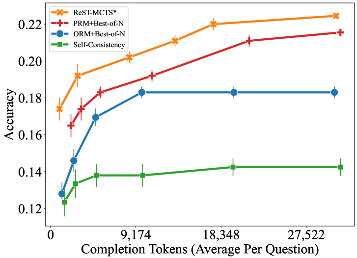</details> (b) Comparison of value model on SciBench. Figure 2: Accuracy of different searches on MATH and SciBench with varied sampling budget. #### 4.2 Evaluating Self-Improvement of ReST-MCTS ∗ In order to thoroughly examine the influence of ReST-MCTS ∗ self-training on varied backbones, we execute 2 iterations of self-training and compare two representative self-training approaches, ReST ${}^EM$ , which compares outcome reward with ground-truth answer, and Self-Rewarding, which judges outcome reward by LLMs, upon 3 different base models, namely LLaMA-3-8B-Instruct [30], Mistral-7B: MetaMATH [29; 31] and SciGLM-6B [10]. Primary results are shown in Table 2. Concerning the dataset for sample generation, since we are primarily interested in the continuous improvement ability of ReST-MCTS ∗ in a specific domain, we mainly include math questions in the dataset. For simplicity, we use the same dataset $D_G$ in each iteration. It involves questions selected from a train set of well-known benchmarks including MATH, GSM8K, and TheoremQA [32]. With the policy and value model trained simultaneously on samples generated from $D_G$ , we observe that our self-training paradigm enables continuous enhancement of the capabilities of both models on in-distribution and out-of-distribution benchmarks, regardless of which backbone is used. $\bullet$ Iterative performance improvement on policy model. Previous LLM self-training approaches mostly rely on the generating responses of LLM and assume each question with the correct solution is a high-quality sample while the intermediate reasoning steps are wrong or useless in many cases. Therefore, we compare the ReST-MCTS ∗ with recent self-training paradigms by generating new samples under different reward (value) supervision strategies. For ReST ${}^EM$ and Self-Rewarding, the default sampling strategy is generating CoT data, with generated data refined according to ground truth or reward provided by the policy, respectively. In comparison, ReST-MCTS ∗ generates data samples via MCTS ∗, with data refined referring to quality value and ground truth. The results in Table 2 show that all three backbones can be continuously self-improved by data generated by itself, using ReST-MCTS ∗ as a paradigm. ReST-MCTS ∗ significantly outperforms previous self-training methods ReST ${}^EM$ and Self-Rewarding basically in each iteration. This means the ReST-MCTS ∗ can screen out self-generated data of higher quality for better self-improvement. $\bullet$ Iterative performance improvement on reward model. We also compare how our iterative trained policy and value model can improve the overall search results under the same token usage on the test set of MATH [33]. See implementation details in Appendix E.3. We show results in Figure 2 (a), where ReST-MCTS ∗ (Iter #1) greatly outperforms most baselines but does not completely surpass Self-Consistency. In comparison, after more iterations of self-training, verification based on the enhanced value model basically outperforms Self-Consistency on every point, achieving the highest accuracy of $48.5\$ that significantly exceeds the $42.5\$ of Self-Consistency. This indicates the effectiveness of our self-training pipeline. Table 3: Accuracy of different verifiers on GSM8K test set and MATH500. SC: Self-Consistency, MS: MATH-SHEPHERD. Verification is based on 256 outputs. | Models | Dataset | SC | ORM | SC+ORM | MS | SC + MS | SC + ReST-MCTS ∗ (Value) | | --- | --- | --- | --- | --- | --- | --- | --- | | Mistral-7B: MetaMATH | GSM8K | 83.9 | 86.2 | 86.6 | 87.1 | 86.3 | 87.5 | | MATH500 | 35.1 | 36.4 | 38.0 | 37.3 | 38.3 | 39.0 | | Table 4: Overall performance comparison with representative models on SciBench. | Models | Subject | Chemistry | Physics | Math | All | | | | | | | | | --- | --- | --- | --- | --- | --- | --- | --- | --- | --- | --- | --- | --- | | Method | atkins | chemmc | quan | matter | fund | class | thermo | diff | stat | calc | Ave. | | | GLM4 | CoT | 11.21 | 23.07 | 8.82 | 4.08 | 19.44 | 2.12 | 7.46 | 10.00 | 12.00 | 28.57 | 12.68 | | ToT | 11.21 | 23.07 | 8.82 | 12.24 | 22.22 | 6.38 | 5.97 | 12.00 | 25.33 | 30.95 | 15.82 | | | ReST-MCTS ∗ | 13.08 | 28.20 | 14.70 | 8.16 | 22.22 | 4.25 | 7.46 | 12.00 | 26.66 | 30.95 | 16.77 | | | GPT-3.5-turbo | CoT | 5.60 | 7.69 | 5.88 | 6.12 | 6.94 | 2.12 | 2.98 | 4.00 | 16.00 | 11.90 | 6.92 | | ToT | 8.41 | 12.82 | 11.76 | 6.12 | 11.11 | 0.00 | 0.00 | 10.00 | 18.66 | 9.52 | 8.44 | | | ReST-MCTS ∗ | 5.60 | 12.82 | 11.76 | 6.12 | 6.94 | 8.51 | 2.98 | 10.00 | 24.00 | 11.90 | 10.06 | | | LLaMA2-13B-Chat | CoT | 2.80 | 2.56 | 2.94 | 2.04 | 2.77 | 2.12 | 0.00 | 2.00 | 2.66 | 2.38 | 2.23 | | ToT | 0.93 | 5.12 | 2.94 | 4.08 | 2.77 | 0.00 | 1.49 | 0.00 | 4.00 | 2.38 | 2.37 | | | ReST-MCTS ∗ | 0.93 | 5.12 | 2.94 | 2.04 | 4.16 | 2.12 | 0.00 | 4.00 | 5.53 | 2.38 | 2.90 | | #### 4.3 Evaluating Reward Guidance and Reasoning Policy of ReST-MCTS ∗ Our main hypothesis in this paper is that a better search policy getting higher-quality traces can improve self-training. In this section, we mainly focus on whether our process reward guided MCTS ∗ can gain improvement to get better samples over different reasoning tasks. We first evaluate the effectiveness of the value model itself standalone in Table 3 and then evaluate the performance of different reasoning policies in Table 4. Performance Comparison of Various Verification Models. As [1] suggested, different value models or reward models vary in accuracy and fineness. We perform tests on the questions of the GSM8K and MATH500 using multiple reward models and verification methods. It is worth noting that we include the same experiment settings of MATH-SHEPHERD (MS) [12] as a comparison since it also adopts an automatic train data generation method for reward models. For SC+ReST-MCTS ∗, we utilize the same CoT-based sampling strategy as MS, except that SC is performed according to our own value model’s output rather than the reward model of MS, which makes this a direct comparison of different reward model training approaches. We record the model accuracy of Mistral-7B: MetaMATH on the selected test set, which is as shown in Table 3. Results indicate that compared to MS and SC+MS, SC+ReST-MCTS ∗ (Value) exhibits higher improvement in solution accuracy on both GSM8K and MATH. This confirms the effectiveness of our value model, further indicating that our definitions of quality value and weighted reward are valid or possibly even better. Performance Comparison under the Same Search Budget. Though the MCTS-based search methods demonstrate significant improvement in model performance, they often require a considerable amount of token input and completion, which makes it quite costly in some circumstances. Therefore, we conduct more experiments to investigate the relationship between search token budget and model performance on science questions selected from SciBench comparing ReST-MCTS ∗ and the same baselines employed for MATH, which are elaborated in Appendix E.3. Since our self-training procedure is primarily conducted on math data, so we do not consider the effects of self-training in this case. However, we point out that this can still be further investigated as a study of transfer learning for self-training paradigms. Figure 2 (b) shows the accuracy of different approaches on SciBench when the completion budget changes. Results indicate that the ReST-MCTS ∗ greatly outperforms other baselines despite insufficient budget. We notice that although CoT-based methods can improve greatly by increasing the sample budget, they tend to quickly converge to a limited accuracy, which is not as satisfying as the ReST-MCTS ∗. Performance Comparison of Different Reasoning Policies on Benchmarks. To evaluate the effectiveness of ReST-MCTS ∗, we perform benchmark experiments on SciBench [34] in Tabel 4 and SciEval [35] in Table 8. All benchmark setups are illustrated in Appendix E.2. For the backbone of models, large-scale models GLM4 and GPT-3.5-turbo (both API), as well as a small-scale model LLaMA2-13B-Chat are included. As shown in Table 4, with the experiment repeated for $2$ times, we report the average accuracy scores (%) of $3$ methods on $10$ subjects. Concerning overall accuracy, the ReST-MCTS ∗ outperforms other baselines for all $3$ models, with GLM4 improved over 4.0% and GPT-3.5-turbo over 3.1%. On specific subjects such as chemmc, quan, and stat, the ReST-MCTS ∗ achieves significant improvement over 5.0%, indicating its great potential in discovering accurate solutions. Besides, we notice that our ToT baseline also performs well on many subjects, sometimes even surpassing ReST-MCTS ∗. This reflects that our value model can provide appropriate guidance for tree-search-based methods. We also discovered that for LLaMA2-13B-Chat, the improvement is not very prominent. This reveals that small-scale policies may face difficulties when adopting complex tree search approaches since their capability for step-wise inference is relatively low. ### 5 Related Work #### 5.1 Large Language Model Training Large Language Models (LLMs) [36; 37; 38] have emerged as a notable success in various natural language tasks. Recent studies focus on improving the reasoning capabilities of LLMs, including collecting high-quality or larger domain-specific data [39; 40; 41; 42; 10; 43], designing elaborate prompting [22; 44; 45; 46], or training supervised learning [10; 31; 32; 47] or reinforcement learning (RL) [48; 49; 50; 16]. When LLMs are trained with the RL algorithm, the generation of LLMs can be naturally expressed as the Markov Decision Process (MDP) and optimized for specific objectives. According to this formula, InstructGPT [51] has achieved remarkable success in optimizing LLMs to align human preferences by utilizing RL from Human Feedback (RLHF) [52]. RLAIF then uses AI feedback to extend RL from human feedback [53]. Our work aims to propose an LLM self-training method via process rewards guided tree search. #### 5.2 Large Language Model Reasoning LLM reasoning algorithms include prompt-based chain-of-thought (CoT) [22], planning-based represented by tree-of-thought (ToT) [24]. Scientific reasoning has several categories to mine the potential of existing large language models, resulting from different performances for problem-solving. Previous studies have attempted to outperform the direct generation. For example, in this paper [54], an approach for generating solutions in a step-by-step manner is proposed, another model or function is used to select the top-ranked answers, and hallucination is avoided by limiting the output to a narrower set. [55] presents a maieutic prompting inference method, which can generate abductive explanations of various hypotheses explained by recursion, eliminate contradicting candidates, and achieve logically consistent reasoning. Chain-of-thoughts (CoT) [22] imitates the thought process like humans to provide step-by-step solutions given a question. Self-Consistency CoT [23] improves the reliability and Self-Consistency of answers by sampling multiple interpretations from LM and then selecting the final answer that appears most frequently. Tree-of-Thoughts (ToT) [24] further generalizes the CoT methodology by considering multiple different reasoning paths in the tree and exploring coherent units of thought to execute thoughtful decision-making. In our work, we benchmark hard science reasoning tasks against [22; 24; 34; 35]. ### 6 Conclusion In this paper, we propose ReST-MCTS ∗, self-training both policy and process reward model by high-quality samples generated by reward guided tree search. Inferred rewards from the previous iteration are able to refine the process reward model and self-train the policy model with high-quality traces. Experimental results show that the ReST-MCTS ∗ outperforms other self-training paradigms and achieves higher accuracy than previous reasoning baselines under the same search budget. Limitation: We discussed limitation in detail at Section H in Appendix. In summary, we need to show the ReST-MCTS ∗ can generalize to other reasoning tasks outside of math (like coding, agent, etc); and tasks without ground-truth (dialogue, SWE-Bench [56], etc). We also need to scale up the proposed value model and further improve the data filtering techniques. One potential idea is to incorporate online RL algorithms that can help perform better self-training for value models and policy models. Acknowledgments Dan and Sining would like to thank Zhipu AI for sponsoring the computation resources used in this work. Yisong is supported in part by NSF #1918655. Yuxiao and Jie are supported in part by the NSFC 62276148, NSFC for Distinguished Young Scholar 62425601, a research fund from Zhipu, New Cornerstone Science Foundation through the XPLORER PRIZE and Tsinghua University (Department of Computer Science and Technology) - Siemens Ltd., China Joint Research Center for Industrial Intelligence and Internet of Things (JCIIOT). Corresponding authors: Yisong Yue, Yuxiao Dong, and Jie Tang. ### References - [1] Hunter Lightman, Vineet Kosaraju, Yura Burda, Harri Edwards, Bowen Baker, Teddy Lee, Jan Leike, John Schulman, Ilya Sutskever, and Karl Cobbe. Let’s verify step by step. arXiv preprint arXiv:2305.20050, 2023. - [2] Yuntao Bai, Saurav Kadavath, Sandipan Kundu, Amanda Askell, Jackson Kernion, Andy Jones, Anna Chen, Anna Goldie, Azalia Mirhoseini, Cameron McKinnon, Carol Chen, Catherine Olsson, Christopher Olah, Danny Hernandez, Dawn Drain, Deep Ganguli, Dustin Li, Eli Tran-Johnson, Ethan Perez, Jamie Kerr, Jared Mueller, Jeffrey Ladish, Joshua Landau, Kamal Ndousse, Kamile Lukosiute, Liane Lovitt, Michael Sellitto, Nelson Elhage, Nicholas Schiefer, Noemí Mercado, Nova DasSarma, Robert Lasenby, Robin Larson, Sam Ringer, Scott Johnston, Shauna Kravec, Sheer El Showk, Stanislav Fort, Tamera Lanham, Timothy Telleen-Lawton, Tom Conerly, Tom Henighan, Tristan Hume, Samuel R. Bowman, Zac Hatfield-Dodds, Ben Mann, Dario Amodei, Nicholas Joseph, Sam McCandlish, Tom Brown, and Jared Kaplan. Constitutional AI: harmlessness from AI feedback. CoRR, abs/2212.08073, 2022. - [3] Zixiang Chen, Yihe Deng, Huizhuo Yuan, Kaixuan Ji, and Quanquan Gu. Self-play fine-tuning converts weak language models to strong language models. CoRR, abs/2401.01335, 2024. - [4] Eric Zelikman, Yuhuai Wu, Jesse Mu, and Noah Goodman. Star: Bootstrapping reasoning with reasoning. Advances in Neural Information Processing Systems, 35:15476–15488, 2022. - [5] Zheng Yuan, Hongyi Yuan, Chengpeng Li, Guanting Dong, Chuanqi Tan, and Chang Zhou. Scaling relationship on learning mathematical reasoning with large language models. arXiv preprint arXiv:2308.01825, 2023. - [6] Avi Singh, John D Co-Reyes, Rishabh Agarwal, Ankesh Anand, Piyush Patil, Peter J Liu, James Harrison, Jaehoon Lee, Kelvin Xu, Aaron Parisi, et al. Beyond human data: Scaling self-training for problem-solving with language models. arXiv preprint arXiv:2312.06585, 2023. - [7] Arian Hosseini, Xingdi Yuan, Nikolay Malkin, Aaron Courville, Alessandro Sordoni, and Rishabh Agarwal. V-star: Training verifiers for self-taught reasoners. arXiv preprint arXiv:2402.06457, 2024. - [8] Mark Chen, Jerry Tworek, Heewoo Jun, Qiming Yuan, Henrique Ponde de Oliveira Pinto, Jared Kaplan, Harri Edwards, Yuri Burda, Nicholas Joseph, Greg Brockman, et al. Evaluating large language models trained on code. arXiv preprint arXiv:2107.03374, 2021. - [9] Yujia Li, David Choi, Junyoung Chung, Nate Kushman, Julian Schrittwieser, Rémi Leblond, Tom Eccles, James Keeling, Felix Gimeno, Agustin Dal Lago, et al. Competition-level code generation with alphacode. Science, 378(6624):1092–1097, 2022. - [10] Dan Zhang, Ziniu Hu, Sining Zhoubian, Zhengxiao Du, Kaiyu Yang, Zihan Wang, Yisong Yue, Yuxiao Dong, and Jie Tang. Sciglm: Training scientific language models with self-reflective instruction annotation and tuning. arXiv preprint arXiv:2401.07950, 2024. - [11] Richard Yuanzhe Pang, Weizhe Yuan, Kyunghyun Cho, He He, Sainbayar Sukhbaatar, and Jason Weston. Iterative reasoning preference optimization. arXiv preprint arXiv:2404.19733, 2024. - [12] Peiyi Wang, Lei Li, Zhihong Shao, RX Xu, Damai Dai, Yifei Li, Deli Chen, Y Wu, and Zhifang Sui. Math-shepherd: A label-free step-by-step verifier for llms in mathematical reasoning. arXiv preprint arXiv:2312.08935, 2023. - [13] Fangkai Jiao, Chengwei Qin, Zhengyuan Liu, Nancy F Chen, and Shafiq Joty. Learning planning-based reasoning by trajectories collection and process reward synthesizing. arXiv preprint arXiv:2402.00658, 2024. - [14] Xidong Feng, Ziyu Wan, Muning Wen, Ying Wen, Weinan Zhang, and Jun Wang. Alphazero-like tree-search can guide large language model decoding and training. arXiv preprint arXiv:2309.17179, 2023. - [15] Richard S Sutton. Learning to predict by the methods of temporal differences. Machine learning, 3:9–44, 1988. - [16] Weizhe Yuan, Richard Yuanzhe Pang, Kyunghyun Cho, Sainbayar Sukhbaatar, Jing Xu, and Jason Weston. Self-rewarding language models. arXiv preprint arXiv:2401.10020, 2024. - [17] Tamera Lanham, Anna Chen, Ansh Radhakrishnan, Benoit Steiner, Carson Denison, Danny Hernandez, Dustin Li, Esin Durmus, Evan Hubinger, Jackson Kernion, et al. Measuring faithfulness in chain-of-thought reasoning. arXiv preprint arXiv:2307.13702, 2023. - [18] Mengzhou Xia, Sadhika Malladi, Suchin Gururangan, Sanjeev Arora, and Danqi Chen. Less: Selecting influential data for targeted instruction tuning. arXiv preprint arXiv:2402.04333, 2024. - [19] Chunting Zhou, Pengfei Liu, Puxin Xu, Srinivasan Iyer, Jiao Sun, Yuning Mao, Xuezhe Ma, Avia Efrat, Ping Yu, Lili Yu, et al. Lima: Less is more for alignment. Advances in Neural Information Processing Systems, 36, 2024. - [20] Julian Schrittwieser, Ioannis Antonoglou, Thomas Hubert, Karen Simonyan, Laurent Sifre, Simon Schmitt, Arthur Guez, Edward Lockhart, Demis Hassabis, Thore Graepel, et al. Mastering atari, go, chess and shogi by planning with a learned model. Nature, 588(7839):604–609, 2020. - [21] Dan Hendrycks, Collin Burns, Saurav Kadavath, Akul Arora, Steven Basart, Eric Tang, Dawn Song, and Jacob Steinhardt. Measuring mathematical problem solving with the math dataset. NeurIPS, 2021. - [22] Jason Wei, Xuezhi Wang, Dale Schuurmans, Maarten Bosma, Fei Xia, Ed Chi, Quoc V Le, Denny Zhou, et al. Chain-of-thought prompting elicits reasoning in large language models. Advances in neural information processing systems, 35:24824–24837, 2022. - [23] Xuezhi Wang, Jason Wei, Dale Schuurmans, Quoc Le, Ed Chi, Sharan Narang, Aakanksha Chowdhery, and Denny Zhou. Self-consistency improves chain of thought reasoning in language models. arXiv preprint arXiv:2203.11171, 2022. - [24] Shunyu Yao, Dian Yu, Jeffrey Zhao, Izhak Shafran, Tom Griffiths, Yuan Cao, and Karthik Narasimhan. Tree of thoughts: Deliberate problem solving with large language models. Advances in Neural Information Processing Systems, 36, 2024. - [25] Karl Cobbe, Vineet Kosaraju, Mohammad Bavarian, Mark Chen, Heewoo Jun, Lukasz Kaiser, Matthias Plappert, Jerry Tworek, Jacob Hilton, Reiichiro Nakano, et al. Training verifiers to solve math word problems. arXiv preprint arXiv:2110.14168, 2021. - [26] Levente Kocsis, Csaba Szepesvári, and Jan Willemson. Improved monte-carlo search. Univ. Tartu, Estonia, Tech. Rep, 1:1–22, 2006. - [27] Zhengxiao Du, Yujie Qian, Xiao Liu, Ming Ding, Jiezhong Qiu, Zhilin Yang, and Jie Tang. Glm: General language model pretraining with autoregressive blank infilling. In Proceedings of the 60th Annual Meeting of the Association for Computational Linguistics (Volume 1: Long Papers), pages 320–335, 2022. - [28] Aohan Zeng, Xiao Liu, Zhengxiao Du, Zihan Wang, Hanyu Lai, Ming Ding, Zhuoyi Yang, Yifan Xu, Wendi Zheng, Xiao Xia, et al. Glm-130b: An open bilingual pre-trained model. arXiv preprint arXiv:2210.02414, 2022. - [29] Albert Q Jiang, Alexandre Sablayrolles, Arthur Mensch, Chris Bamford, Devendra Singh Chaplot, Diego de las Casas, Florian Bressand, Gianna Lengyel, Guillaume Lample, Lucile Saulnier, et al. Mistral 7b. arXiv preprint arXiv:2310.06825, 2023. - [30] Meta AI. Meta llama 3. https://ai.meta.com/blog/meta-llama-3/, 2024. Accessed: 2024-05-22. - [31] Longhui Yu, Weisen Jiang, Han Shi, Jincheng Yu, Zhengying Liu, Yu Zhang, James T Kwok, Zhenguo Li, Adrian Weller, and Weiyang Liu. Metamath: Bootstrap your own mathematical questions for large language models. arXiv preprint arXiv:2309.12284, 2023. - [32] Xiang Yue, Xingwei Qu, Ge Zhang, Yao Fu, Wenhao Huang, Huan Sun, Yu Su, and Wenhu Chen. Mammoth: Building math generalist models through hybrid instruction tuning. arXiv preprint arXiv:2309.05653, 2023. - [33] Dan Hendrycks, Collin Burns, Saurav Kadavath, Akul Arora, Steven Basart, Eric Tang, Dawn Song, and Jacob Steinhardt. Measuring mathematical problem solving with the math dataset. arXiv preprint arXiv:2103.03874, 2021. - [34] Xiaoxuan Wang, Ziniu Hu, Pan Lu, Yanqiao Zhu, Jieyu Zhang, Satyen Subramaniam, Arjun R Loomba, Shichang Zhang, Yizhou Sun, and Wei Wang. Scibench: Evaluating college-level scientific problem-solving abilities of large language models. arXiv preprint arXiv:2307.10635, 2023. - [35] Liangtai Sun, Yang Han, Zihan Zhao, Da Ma, Zhennan Shen, Baocai Chen, Lu Chen, and Kai Yu. Scieval: A multi-level large language model evaluation benchmark for scientific research. arXiv preprint arXiv:2308.13149, 2023. - [36] Josh Achiam, Steven Adler, Sandhini Agarwal, Lama Ahmad, Ilge Akkaya, Florencia Leoni Aleman, Diogo Almeida, Janko Altenschmidt, Sam Altman, Shyamal Anadkat, et al. Gpt-4 technical report. arXiv preprint arXiv:2303.08774, 2023. - [37] Gemini Team, Rohan Anil, Sebastian Borgeaud, Yonghui Wu, Jean-Baptiste Alayrac, Jiahui Yu, Radu Soricut, Johan Schalkwyk, Andrew M Dai, Anja Hauth, et al. Gemini: a family of highly capable multimodal models. arXiv preprint arXiv:2312.11805, 2023. - [38] Team GLM, Aohan Zeng, Bin Xu, Bowen Wang, Chenhui Zhang, Da Yin, Diego Rojas, Guanyu Feng, Hanlin Zhao, Hanyu Lai, et al. Chatglm: A family of large language models from glm-130b to glm-4 all tools. arXiv preprint arXiv:2406.12793, 2024. - [39] Hugo Touvron, Thibaut Lavril, Gautier Izacard, Xavier Martinet, Marie-Anne Lachaux, Timothée Lacroix, Baptiste Rozière, Naman Goyal, Eric Hambro, Faisal Azhar, et al. Llama: Open and efficient foundation language models. arXiv preprint arXiv:2302.13971, 2023. - [40] Hugo Touvron, Louis Martin, Kevin Stone, Peter Albert, Amjad Almahairi, Yasmine Babaei, Nikolay Bashlykov, Soumya Batra, Prajjwal Bhargava, Shruti Bhosale, et al. Llama 2: Open foundation and fine-tuned chat models. arXiv preprint arXiv:2307.09288, 2023. - [41] Ross Taylor, Marcin Kardas, Guillem Cucurull, Thomas Scialom, Anthony Hartshorn, Elvis Saravia, Andrew Poulton, Viktor Kerkez, and Robert Stojnic. Galactica: A large language model for science. arXiv preprint arXiv:2211.09085, 2022. - [42] Suriya Gunasekar, Yi Zhang, Jyoti Aneja, Caio César Teodoro Mendes, Allie Del Giorno, Sivakanth Gopi, Mojan Javaheripi, Piero Kauffmann, Gustavo de Rosa, Olli Saarikivi, et al. Textbooks are all you need. arXiv preprint arXiv:2306.11644, 2023. - [43] Xue Lilong, Zhang Dan, Dong Yuxiao, and Tang Jie. Autore: Document-level relation extraction with large language models. arXiv preprint arXiv:2403.14888, 2024. - [44] Denny Zhou, Nathanael Schärli, Le Hou, Jason Wei, Nathan Scales, Xuezhi Wang, Dale Schuurmans, Claire Cui, Olivier Bousquet, Quoc Le, et al. Least-to-most prompting enables complex reasoning in large language models. arXiv preprint arXiv:2205.10625, 2022. - [45] Jiale Cheng, Xiao Liu, Kehan Zheng, Pei Ke, Hongning Wang, Yuxiao Dong, Jie Tang, and Minlie Huang. Black-box prompt optimization: Aligning large language models without model training. arXiv preprint arXiv:2311.04155, 2023. - [46] Antonia Creswell, Murray Shanahan, and Irina Higgins. Selection-inference: Exploiting large language models for interpretable logical reasoning. arXiv preprint arXiv:2205.09712, 2022. - [47] Aohan Zeng, Mingdao Liu, Rui Lu, Bowen Wang, Xiao Liu, Yuxiao Dong, and Jie Tang. Agenttuning: Enabling generalized agent abilities for llms. arXiv preprint arXiv:2310.12823, 2023. - [48] Hanze Dong, Wei Xiong, Deepanshu Goyal, Rui Pan, Shizhe Diao, Jipeng Zhang, Kashun Shum, and Tong Zhang. Raft: Reward ranked finetuning for generative foundation model alignment. arXiv preprint arXiv:2304.06767, 2023. - [49] Caglar Gulcehre, Tom Le Paine, Srivatsan Srinivasan, Ksenia Konyushkova, Lotte Weerts, Abhishek Sharma, Aditya Siddhant, Alex Ahern, Miaosen Wang, Chenjie Gu, et al. Reinforced self-training (rest) for language modeling. arXiv preprint arXiv:2308.08998, 2023. - [50] Rafael Rafailov, Archit Sharma, Eric Mitchell, Christopher D Manning, Stefano Ermon, and Chelsea Finn. Direct preference optimization: Your language model is secretly a reward model. Advances in Neural Information Processing Systems, 36, 2024. - [51] Long Ouyang, Jeffrey Wu, Xu Jiang, Diogo Almeida, Carroll Wainwright, Pamela Mishkin, Chong Zhang, Sandhini Agarwal, Katarina Slama, Alex Ray, et al. Training language models to follow instructions with human feedback. Advances in neural information processing systems, 35:27730–27744, 2022. - [52] Paul F Christiano, Jan Leike, Tom Brown, Miljan Martic, Shane Legg, and Dario Amodei. Deep reinforcement learning from human preferences. Advances in neural information processing systems, 30, 2017. - [53] Harrison Lee, Samrat Phatale, Hassan Mansoor, Kellie Lu, Thomas Mesnard, Colton Bishop, Victor Carbune, and Abhinav Rastogi. Rlaif: Scaling reinforcement learning from human feedback with ai feedback. arXiv preprint arXiv:2309.00267, 2023. - [54] Antonia Creswell and Murray Shanahan. Faithful reasoning using large language models. arXiv preprint arXiv:2208.14271, 2022. - [55] Jaehun Jung, Lianhui Qin, Sean Welleck, Faeze Brahman, Chandra Bhagavatula, Ronan Le Bras, and Yejin Choi. Maieutic prompting: Logically consistent reasoning with recursive explanations. arXiv preprint arXiv:2205.11822, 2022. - [56] Carlos E Jimenez, John Yang, Alexander Wettig, Shunyu Yao, Kexin Pei, Ofir Press, and Karthik Narasimhan. Swe-bench: Can language models resolve real-world github issues? arXiv preprint arXiv:2310.06770, 2023. - [57] Tom Brown, Benjamin Mann, Nick Ryder, Melanie Subbiah, Jared D Kaplan, Prafulla Dhariwal, Arvind Neelakantan, Pranav Shyam, Girish Sastry, Amanda Askell, et al. Language models are few-shot learners. Advances in neural information processing systems, 33:1877–1901, 2020. - [58] Maciej Besta, Nils Blach, Ales Kubicek, Robert Gerstenberger, Michal Podstawski, Lukas Gianinazzi, Joanna Gajda, Tomasz Lehmann, Hubert Niewiadomski, Piotr Nyczyk, et al. Graph of thoughts: Solving elaborate problems with large language models. In Proceedings of the AAAI Conference on Artificial Intelligence, volume 38, pages 17682–17690, 2024. - [59] Shibo Hao, Yi Gu, Haodi Ma, Joshua Jiahua Hong, Zhen Wang, Daisy Zhe Wang, and Zhiting Hu. Reasoning with language model is planning with world model. arXiv preprint arXiv:2305.14992, 2023. - [60] David Silver, Julian Schrittwieser, Karen Simonyan, Ioannis Antonoglou, Aja Huang, Arthur Guez, Thomas Hubert, Lucas Baker, Matthew Lai, Adrian Bolton, et al. Mastering the game of go without human knowledge. nature, 550(7676):354–359, 2017. - [61] Ye Tian, Baolin Peng, Linfeng Song, Lifeng Jin, Dian Yu, Haitao Mi, and Dong Yu. Toward self-improvement of llms via imagination, searching, and criticizing. arXiv preprint arXiv:2404.12253, 2024. - [62] Ilya Loshchilov and Frank Hutter. Decoupled weight decay regularization. arXiv preprint arXiv:1711.05101, 2017. - [63] Cameron B Browne, Edward Powley, Daniel Whitehouse, Simon M Lucas, Peter I Cowling, Philipp Rohlfshagen, Stephen Tavener, Diego Perez, Spyridon Samothrakis, and Simon Colton. A survey of monte carlo tree search methods. IEEE Transactions on Computational Intelligence and AI in games, 4(1):1–43, 2012. - [64] Hongming Zhang and Tianyang Yu. Alphazero. Deep Reinforcement Learning: Fundamentals, Research and Applications, pages 391–415, 2020. - [65] Henry W Sprueill, Carl Edwards, Mariefel V Olarte, Udishnu Sanyal, Heng Ji, and Sutanay Choudhury. Monte carlo thought search: Large language model querying for complex scientific reasoning in catalyst design. arXiv preprint arXiv:2310.14420, 2023. - [66] Jiacheng Liu, Andrew Cohen, Ramakanth Pasunuru, Yejin Choi, Hannaneh Hajishirzi, and Asli Celikyilmaz. Don’t throw away your value model! making ppo even better via value-guided monte-carlo tree search decoding. arXiv e-prints, pages arXiv–2309, 2023. ## Appendix ### Appendix A Preliminaries In this section, we briefly describe LLM reasoning, reward verification, and LLM self-training. The definitions for notations are in Table 5 and model comparison in Figure 6. Table 5: Notation Table. | Character | Meaning | | --- | --- | | $Q$ | given question/problem | | $A$ | decoded answer | | $a^*$ | final correct answer | | $s$ | solution | | $p$ | partial solution | | $s_k$ | $k$ -th step of solution $s$ | | $K$ | number of reasoning steps of a solution | | $A_j$ | $j$ -th solution | | $N$ | number of solutions | | $d$ | number of preference pairs | | $r_s_{k}$ | common PRM reward of a single step $s_k$ , used to define weighted reward | | $w_s_{k}$ | weighted reward of a single step $s_k$ , inferred in self-training process after trace generation | | $v_k$ | quality value of partial steps $p_k$ , used to guide search; inferred in self-training process | | $m_k$ | reasoning distance of partial steps $p_k$ | | $π_B$ | base language model | | $D_S_0$ | original training dataset | | $V_θ$ | process reward model | | $r_φ$ | outcome reward model | #### A.1 LLM Reasoning The use of reasoning approaches can significantly improve LLM problem-solving abilities [10]. Given a policy model, $π$ (an autoregressive pre-trained language model) and an input problem $Q$ , $π$ can autoregressive generate an output sequence $s=(s_1,s_2,⋯,s_K)$ by predicting the next token. The conditional probability distribution of generating the complete output sequence is: $$ π(s|Q)=∏_k=1^Kπ(s_t|s_<t,Q). \tag{5} $$ Any problem can be reasoned by zero-shot prompting, few-shot prompting [57], chain-of-thought (CoT) [22], self-consistency CoT [23] or best-of-N (BoN) selection [1], tree-of-thought (ToT) [24], Monte Carlo tree search (MCTS) [14], graph-of-thought (GoT) [58], amongst other approaches. Generally, recent studies represented by CoT [22] aim to improve the overall performance as follows: $$ P_π(A=a^*\mid Q)=E_(s_{0,s_1,⋯,s_K)∼ P_π(s \mid Q)}\Big{[}P(A=a^*\mid s_0,s_1,⋯,s_K,Q)\Big{]}. \tag{6} $$ We often call each trajectory $(s_1,s_2,⋯,s_K)$ a reasoning trace. $P(A=a^*\mid s_0,s_1\dots,s_K,Q)$ is the probability to get correct answer $a^*$ given a problem $Q$ and a reasoning trace $s$ . Given a original training dataset $D=\{Q_1,Q_2,⋯,Q_M\}$ , a new dataset can be produced by sampling $π$ $N$ times per problem Q using the above-mentioned reasoning strategies: $$ D_S_0=\{(Q_1^j,s_1^j)|^N_j=1,⋯,(Q_M^j,s_M^j)|^N _j=1\}. \tag{7} $$ As shown in Table 1, STaR [4], RFT [5], $ReST^EM$ [6], V-STaR [7], and Self-Rewarding [16] adopt CoT prompting. Step-by-step [1] and MATH-SHEPHERD [12] leverage the best-of-N selection as a reasoning evaluation strategy. TS-LLM [14] utilizes MCTS as a reasoning policy to fully generate traces. Our work similarly seeks a correct reasoning path to maximize the expected cumulative $P$ . #### A.2 Reward Verification In the context of LLMs, we assume that the reasoning trajectory is derived from the policy model $π$ sampling. The common first step of self-training methods is fine-tuning the base model $π$ on the original dataset $D_S_0$ and obtaining a new generator $π_S_0$ . Besides, a reward $r$ is considered to evaluate the value of the history trace. The objective of reinforcement learning (RL) with reward $r(Q,s)$ is: $$ L_RL=E_Q∈ D_{S_0}[E_s∈π(s|Q)[ r(Q,s)]]. \tag{8} $$ Recent works [1, 12], through PRMs and ORMs, model the objective of reasoning as a search to find the highest cumulative reward trajectory $s$ to a problem $Q$ and infer the final answer $A$ . $\bullet$ ORM ( $D× S→ℝ$ ) is trained with a cross-entropy loss: $$ L_ORM=A_slog r_s+(1-A_s) log(1-r_s), \tag{9} $$ where $A_s$ is the golden answer ( $A_s=1$ if $s$ is correct else $A_s=0$ ) and $r_s$ is the ORM’s output sigmoid score. STaR [4], RFT [5], and $ReST^EM$ [6] consider the outcome reward as value label $A_s$ compared with ground truth answer. In V-STaR [7], its outcome reward is generated by multi-iteration LLMs, and reward $r$ is defined via verifier $π_V$ and LLM generator $π_S_0$ as follows: $$ r(Q,s)=β log\frac{π_V(s|Q)}{π_S_0(s|Q)}. \tag{10} $$ $β$ is the hyper-parameter that controls the proximity of the reference policy $π_S_0$ . Different from V-STaR, the outcome rewards $r$ in self-rewarding [16] is generated through LLM-as-a-Judge prompting using dataset $D_S_0$ and policy model $π_S_0$ . In both V-STaR and self-rewarding, collected $D_VER$ is built for training verifiers as follows: $$ D_VER=\{(Q_j,s_j,1^+,s_j,1^-),⋯,(Q_j,s_j,d^+,s_ j,d^-)\}^N_j=1, \tag{11} $$ $d$ is the number of preference pairs. However, previous works [1, 12] suggested PRMs demonstrate better supervision than ORMs among false positive solutions and provide more reliable feedback. $\bullet$ PRM ( $D× S→ℝ^+$ ) is trained with: $$ L_PRM=∑\limits_i=1^KA_s_{k}log r_s_{k}+( 1-A_s_{k}) log(1-r_s_{k}), \tag{12} $$ where $A_s_{k}$ is the golden answer ( $A_s_{k}=1$ if $s_k$ is correct else $A_s_{k}=0$ ) of $s_k$ and $r_s_{k}$ is the PRM’s output sigmoid score. Specifically, [1] regards PRM training as a three-class classification with costly human annotations. Similarly, MATH-SHEPHERD [12] collects random rollout trajectories via BoN reasoning policy and synthesizes process rewards to construct the PRM training dataset autonomously. MATH-SHEPHERD defines the automated quality $r_s_{k}$ , the potential to deduce the correct answer, for each reasoning step $s_k$ through hard estimation (HE) and soft estimation (SE), which are, $$ A_s_{k}^HE=≤ft\{\begin{array}[]{cc}1,&∃ A_j∈ A^*,A_j =a^*\\ 0,&Otherwise\end{array}\right., \tag{13} $$ $$ and A_s_{k}^SE=\frac{Σ_j=1^NI(A_j=a ^*)}{N}. \tag{14} $$ $A^*=\{A_j\}^N_j=1$ and $N$ is the number of solutions. To more precisely find a reasoning trajectory with the highest expected reward, RAP [59] utilizes MCTS to estimate the expected future reward via state-action function ( $Q:S×A\longmapstoℝ$ ) in traditional RL for each node. However, the decoding process of incorporating MCTS into LLMs is costly, because estimating and updating a state-action function requires a recursive visit, and reward values need to be calculated by LLMs. The concurrent work pDPO [13], though effective, does not take internal accuracy generated by LLMs into account and ignores the number of steps to be generated. In this paper, we integrate process reward guidance with tree search to explore efficient solution space and synthesize high-quality trajectories. #### A.3 LLM Self-Training Generation. Given a new training dataset $D_G$ , self-training methods use generator $π_S_0$ to generate reasoning steps $s$ and final answer $A$ per problem $Q$ . In each iteration $i$ ( $i≥ 1$ ), STaR, RFT, and ReST ${}^EM$ check the generated solutions $D_G_{i}$ with the binary correctness label $z$ and keeps the correct solutions $(A_j=a^*)|_j=1^N$ as $D_G_{i(A_j=a^*)|_j=1^N}$ . Based on the continuous iteration on positive samples, V-STaR and Self-Rewarding keep the correct and incorrect generated solutions per problem $Q$ and train preference data pairs on constructed verifier data $D_VER$ with all data $D_G_{i}$ , so the $π_V$ can learn the error patterns produced by a generator in each iteration $i$ . Then, the generator $π_S_{i-1}$ , here is $π_S_0$ , is fine-tuned on new generated dataset $D_G_{i(A_j=a^*)|_j=1^N}$ and again is updated as generator $π_S_{i}$ . This process is continuously running in subsequent iterations. Their iterative process and reward value are as follows: $$ D_S_0\xrightarrow{π}π_S_0\xrightarrow{D_G}D_G_{i(A_j=a^*)} \xrightarrow{π_S_{i-1}}π_S_{i}, \tag{15} $$ where $i=1$ for RFT and $i≥ 1$ for STaR, ReST ${}^EM$ , V-STaR, and Self-Rewarding. Improvement. The practical way to accomplish reasoning tasks on $D_S_0$ is supervised fine-tuning (SFT) that trains a policy model by minimizing the negative log-likelihood loss on the training dataset: $$ L_SFT(π)=-E_(Q,s)∈ D_{S_0}\big{[}∑ \limits_t=1^Tlogπ(s_t|s_<t,Q)\big{]}. \tag{16} $$ Recent offline preference learning methods replace LLM verifiers (before being trained on LLM generator and binary classification) with DPO [50]. The training DPO objective for a verifier $π_V$ is described as follows: $$ L_DPO(π_V;π_S_0)=-E_(Q,s^+,s^{-)∼ D _VER}[log σ(r(Q,s^+)-r(Q,s^-))], \tag{17} $$ where $σ$ is the logistic function. ### Appendix B Deduction Demonstration #### B.1 Definition of Weighted Value and Quality Value Weighted Value. Recall the definition of the weighted reward: $$ w_s_{k}=\frac{1-v_k-1}{m_k+1}(1-2r_s_{k}), k=1,2,⋯ \tag{18} $$ And we know that $r_s_{k}∈[0,1]$ . Now, let’s examine the maximum possible value of the term $(1-2r_s_{k})$ . Since $r_s_{k}∈[0,1]$ , the maximum value of $(1-2r_s_{k})$ occurs when $r_s_{k}=0$ . In this case, $(1-2r_s_{k})=1$ . Therefore, we can conclude that $-1≤(1-2r_s_{k})≤ 1$ . Next, let’s consider the denominator, $(m_k+1)$ . Since $m_k=K-k$ , and $K≥ k$ , we have $m_k≥ 0$ and $m_k+1≥ 1$ . Therefore, we can conclude that $(m_k+1)≥ 1$ . Combining these results, we can rewrite the weighted reward as follows: $$ w_s_{k}=\frac{1-v_k-1}{m_k+1}(1-2r_s_{k})≤|1-v_k-1|·|1-2r_s_ {k}|≤|1-v_k-1| \tag{19} $$ Hence, we deduce that $w_s_{k}≤|1-v_k-1|$ , which indicates that the weighted reward is bounded by the absolute value of the difference between 1 and the previous quality value. Quality Value. Recall that the quality value $v_k$ is determined by incorporating the previous quality value $v_k-1$ and the weighted reward $w_s_{k}$ of the current step. $$ v_k=max(v_k-1+w_s_{k},0) \tag{20} $$ Now, we can inductively reach the conclusion that $v_k∈[0,1]$ , starting from the fact that $v_0=0$ . Assuming that $v_k-1∈[0,1]$ , then we can derive $v_k∈[0,1]$ using the bound of $w_s_{k}$ . $$ v_k=max(v_k-1+w_s_{k},0)≤ v_k-1+|1-v_k-1|=1 \tag{21} $$ Therefore, based on the properties of the weighted reward and the definition of the quality value, we can deduce that $v_k$ is indeed confined within the range $[0,1],k=0,1,2,⋯$ . Fine-grained Dataset for Math. We adopt an alternative method to generate value train data for math. For this method, we only demand a correct final answer $a_*$ for each question $q$ , which is simpler to satisfy. Specifically, we integrate the MATH [33] train set into $D_0$ . For each question $q^(i)$ and answer $a^(i)_*$ , we use Mistral-7B: MetaMATH [31] as a policy to generate solution traces in a simple breadth-first-search (BFS) manner, obtaining a search tree $T_q^(i)$ similar to the one of the self-training process. Subsequently, we verify the obtained answers of all leaf nodes of $T_q^(i)$ according to $a_*^(i)$ . The verified search trees are then used to derive data samples with target values for $D_V_0$ . $\bullet$ Construction of value model training set. Previous approaches like [1] that employ PRMs usually require human annotation to initialize a train set, which is quite costly. In comparison, our value model’s initial training set can be constructed at a lower expense. For math data, we deploy the same approach mentioned in section 3.2 to infer process rewards and quality values of partial solutions within the verified search tree $T_q^(i)$ . While for science data, this value-inferring process is slightly different. We still derive the target value of $p_k^(i)$ based on the definition in Eq. (3) and Eq. (4). Under the assumption that original solutions are reliable and concise, we can simply regard $s^(i)$ as the globally optimal reasoning path for $q^(i)$ . Therefore, we derive that: $$ r_s_{k}^(i)=0,m_k^(i)=K_i-k,w_k^(i)=\frac{1}{K_i} and v_k^(i)=\frac{k}{K_i}. \tag{22} $$ Derivation. Please refer to the detailed derivation for Eq. (22) in Appendix B.2. In contrast, for generated false samples, we set $r_s_{k+1}^(i)^{\prime}=1$ , $m_k+1^(i)^{\prime}=K_i-k$ (since still $K_i-k$ correct reasoning steps required to reach final answer). Considering that $v_k^(i)=\frac{k}{K_i}$ , we have: $$ w_k+1^(i)^{\prime}=-\frac{K_i-k}{K_i-k+1}\frac{1}{K_i}, \tag{23} $$ $$ v_k+1^(i)^{\prime}=\max(0,\frac{k-1}{K_i}+\frac{1}{K_i·(K_i-k+1) }). \tag{24} $$ Derivation. Please refer to the detailed derivation for Eq. (23) and Eq. (24) in Appendix B.2. Collecting all samples and their corresponding derived quality values, we acquire the initial training set $D_V_0$ for value model $V_θ$ , as described in Appendix E.1. #### B.2 Detailed Deduction for Weighted Value and Quality Value Here, we deduce the weighted reward using Eq. (4) and quality value using Eq. (3): when $k=0$ : $$ v_0=0 \tag{25} $$ when $k=1$ : $$ \displaystyle w_1=\frac{1-0}{K-1+1}(1-2× 0)=\frac{1}{K} \displaystyle v_1=\max(0+\frac{1}{K},0)=\frac{1}{K} \tag{26} $$ when $k=2$ : $$ \displaystyle w_2=\frac{1-\frac{1}{K}}{K-2+1}(1-2× 0)=\frac{K-1}{K(K-1) }=\frac{1}{K} \displaystyle v_2=\max(\frac{1}{K}+\frac{1}{K},0)=\frac{2}{K} \tag{28} $$ therefore, $$ \displaystyle w_k=\frac{1}{K},w_k-1=\frac{1}{K},w_k+1=\frac{1}{K} \displaystyle v_k=\frac{k}{K},v_k-1=\frac{k-1}{K},v_k+1=\frac{k+1}{K} \displaystyle m_k=K-k,m_k-1=K-k+1,m_k+1=K-k-1. \tag{30} $$ Then, we deduce the Eq. (23) and Eq. (24): $$ \displaystyle w_k+1 \displaystyle=\frac{1-v_k}{m_k+1+1}(1-2r_s_{k+1}) \displaystyle=\frac{1-\frac{k}{K}}{(K-k)+1}(1-2× 1) \displaystyle=-\frac{K-k}{K(K-k+1)} \displaystyle=-\frac{1}{K}\frac{K-k}{K-k+1} \tag{33} $$ $$ \displaystyle v_k+1 \displaystyle=\max(v_k+w_k+1,0) \displaystyle=\max(\frac{k}{K}-\frac{1}{K}\frac{K-k}{K-k+1},0) \displaystyle=\max(\frac{k(K-k+1)-(K-k)}{K(K-k+1)},0) \displaystyle=\max(\frac{k(K-k+1)-(K-k+1)+1}{K(K-k+1)},0) \displaystyle=\max(\frac{(K-k+1)(k-1)+1}{K(K-k+1)},0) \displaystyle=\max(\frac{(K-k+1)(k-1)}{K(K-k+1)}+\frac{1}{K(K-k+1)},0) \displaystyle=\max(\frac{k-1}{K}+\frac{1}{K(K-k+1)},0) \tag{34} $$ ### Appendix C Algorithm Detail and Process Example #### C.1 Algorithm Details of MCTS ∗ 0: question $q$ , inference $\_$ model $π_S_0$ , value $\_$ model $V_θ$ , max $\_$ iterations $T$ , threshold $l$ , branch $b$ , rollout $\_$ steps $m$ , roll $\_$ branch $d$ , weight $\_$ parameter $α$ . 1: $T_q←$ Initialize $\_$ tree $(q)$ 2: $π_S_0,V_θ←$ Initialize $\_$ models $(π_S_0,V_θ)$ 3: for $i$ in range $(T)$ do 4: $C←$ root $(T_q)$ 5: —————Node Selection————— 6: while $C$ is not leaf node do 7: $C← argmax_C^{^{\prime}∈children(C)}(v_C^{^{\prime}}+ ε√{\frac{\ln{n_C}}{n_C^{^{\prime}}}})$ // Select child node based on UCB 8: end while 9: if $v_C≥ l$ then 10: Return $p_C$ // Output solution 11: end if 12: —————Self-Critic————— 13: $o←$ Do $\_$ self $\_$ critic $(p_C|q,π_S_0)$ // Get $π_S_0$ response for further exploitation or stop reasoning 14: if $o$ is not EoI then 15: —————Thought Expansion————— 16: for $j$ in range( $b$ ) do 17: $C_j←$ Get $\_$ new $\_$ child( $o,p_C|q,π_S_0$ ) // Expand based on previous steps and self-critic 18: $v_C_{j}← V_θ(p_C_{j}|q)$ // Evaluate with value model 19: end for 20: —————Greedy MC Rollout————— 21: $C^{^\prime}← argmax_C^{^{\prime}∈children(C)}(v_C^ {^{\prime}}$ ) 22: $p=p_C^{^{\prime}}$ 23: $v_max=0$ 24: for $k$ in range( $m$ ) do 25: $p,v_max←$ Get $\_$ next $\_$ step $\_$ with $\_$ best $\_$ value( $p|π_S_0,V_θ,d,q)$ // Sample new children and record the best-observed value 26: end for 27: $v_C^{^{\prime}}←α v_C^{^{\prime}}+(1-α)v_max$ 28: $n_C^{^{\prime}}← n_C^{^{\prime}}+1$ // Update value and visit count of the rollout node 29: end if 30: —————Value Backpropagation————— 31: Back $\_$ propagate( $C$ ) // Update value of parent nodes using weighted average 32: end for 33: $C$ =Get $\_$ best $\_$ node( $T_q$ ) // Fetch the node with the highest value in the search tree 34: Return $p_C$ 34: $p_C$ Algorithm 2 The proposed value guided search algorithm MCTS ∗. Node Selection. Similar to [14], we propose to start each selection process from the initial root, since this allows backtracking. Within each iteration, the node selection stage is first executed, where a leaf node $C_select$ is hierarchically selected starting from the initial root. To incorporate the quality value of nodes, we use UCB as the criterion to select a child rather than the UCT [26], which is as follows: $$ UCB(C)=v_C+ε√{\frac{\ln{n_parent}}{n_C}}, \tag{35} $$ where $n_parent$ is the number of visits of the parent node of $C$ , $ε$ is a exploration constant. For each intermediate node, we select its child with maximum UCB. This criterion considers both quality value and visit count, thus it encourages the exploration of high-quality nodes while leaving some opportunity for underexplored nodes. Thought Expansion. Secondly, the value of the selected node $C_select$ is compared with a threshold $l$ (in our experiments, $l$ it is set to $0.9$ ). If the $v_C_{select}>=l$ , the node’s recorded partial solution $p_C_{select}=[s_1,s_2,⋯,s_k]$ is deemed acceptable as a final solution (since $v_C$ get close to $1$ only when $C$ is close to correct final answer), which is then directly returned as output, terminating the algorithm. This is different from the method adopted by [60] since no reward model estimation is required. Otherwise, the expansion stage is initiated, where new solution steps $s_k+1,i(i=1,2,⋯,b)$ are sampled by prompting the policy $π_S_0$ , i.e. $s_k+1,i∼π_S_0(s_1,2,⋯,k|q)$ , $b$ is the number of samples or branches. Subsequently, new nodes $C_i=([s_1,s_2,⋯,s_k,s_k+1,i],0,v_C_{i})$ are added to $T_q$ with $v_C_{i}$ assigned by the value model, $v_C_{i}← V_θ(p_C_{i}|q)$ . Note that we also incorporate a self-critic mechanism into this expansion process, which will be illustrated later. Greedy MC Rollout. [60] and [14] use a simplified three-stage iteration that doesn’t include a simulation process on leaf nodes. In contrast, we believe that a simulation process still brings about useful information for value estimation, despite the rise in generation and time cost. In this stage, we propose to simulate a few steps upon the new node $C_i$ with maximum predicted value. Reasoning steps starting from this node will be sampled step-by-step and evaluated, while only the most valuable path is further explored, until a step limit $m$ is reached. The highest quality value acquired in the sampling process $v_max$ is recorded and used to update $v_C_{i}$ with a weight parameter $α$ following: $$ v_C_{i}←α v_C_{i}+(1-α)v_max. \tag{36} $$ Besides, the visit count $n_C_{i}$ is also updated by $n_C_{i}← n_C_{i}+1$ . Value Backpropagation. Finally, we conduct value backup starting from $C_select$ . The value of every parent node of $C_select$ is updated using a weighted average method. For every node $C$ on the trace from root to $C_select$ , we update its $n_C$ and $v_C$ as follows: $$ n_C← n_C+1 \tag{37} $$ and $$ v_C←\frac{Σ_in_C_{i}· v_C_{i}}{Σ_in_C_{i}} \tag{38} $$ where $C_i(i=1,2,⋯,b)$ are the children of $C$ . This actually updates the value of $C$ according to its children’s value expectation. Determine Termination via Self-Critic. Although the value model provides accurate evaluation for partial solutions, it cannot consistently signal logical termination, especially when the inference model reaches a false conclusion. Consequently, even when a false final answer is generated, further exploration beneath this node may still be conducted, leading to reduced search efficiency. Therefore, we propose to use self-critic to provide extra timely signals of logical termination that avoid unwise exploration as well as insight into deeper search. Specifically, we prompt the inference model to generate an End of Inference (EoI) signal or offer advice $o$ on following exploration steps based on existing partial solutions $p$ before each expansion stage. The expansion and MC rollout stage will be skipped if an EoI signal is received. Otherwise, the advice will be utilized in the following expansion stage as part of the inference prompt, so $π_S_0$ generates new steps based on both $o$ and $p$ . An overall pseudo-code for ReST-MCTS ∗ is presented in Algorithm 2. 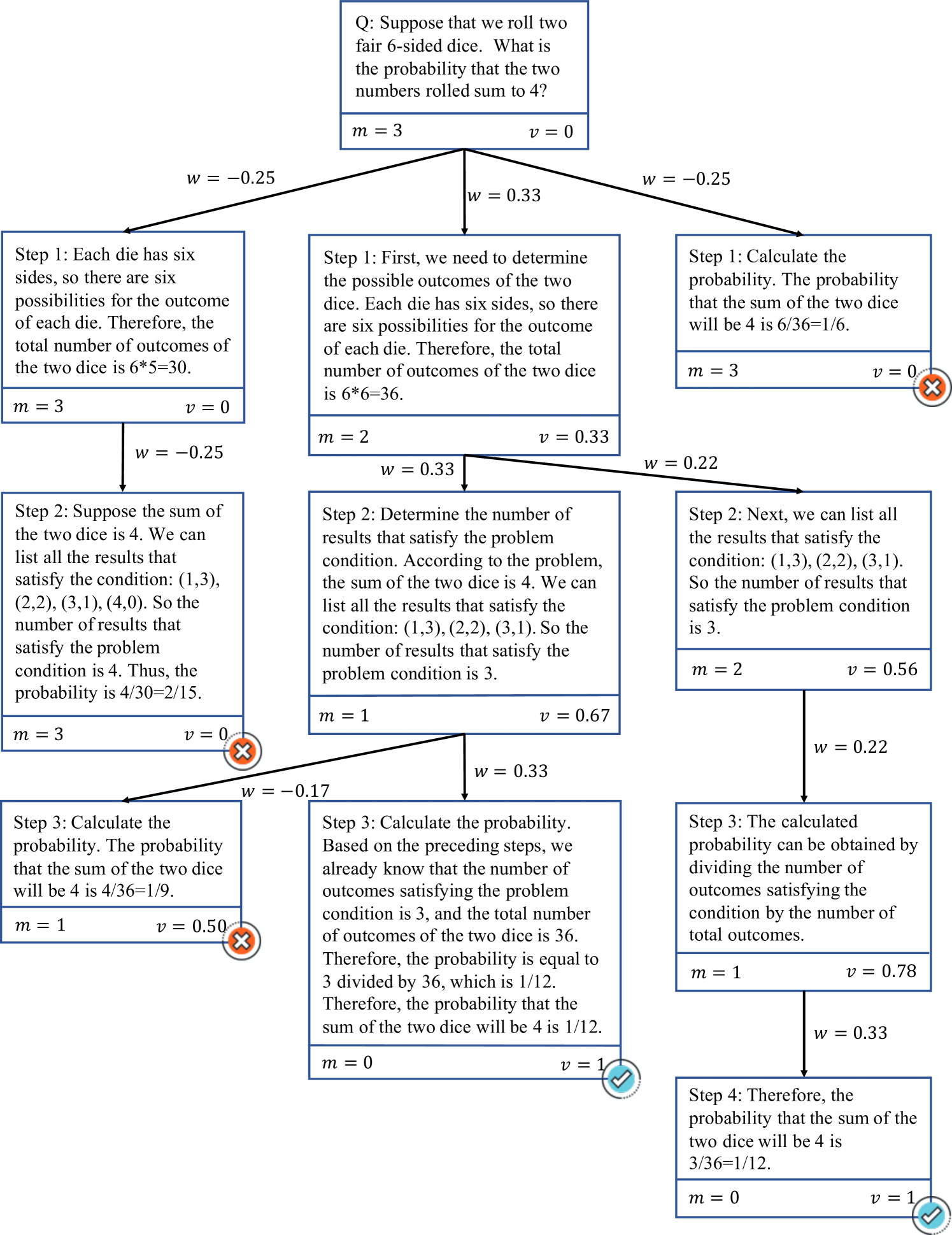<details> <summary>x4.png Details</summary>  ### Visual Description ## Decision Tree Diagram: Probability Problem Solution Paths ### Overview The image displays a decision tree diagram that illustrates three different reasoning paths for solving a probability problem. The central question is presented at the top, and three distinct solution approaches branch downward. Each path consists of sequential steps (Step 1, Step 2, etc.) contained within blue-bordered boxes. The diagram includes numerical annotations (`m`, `v`, `w`) on the boxes and connecting arrows, and uses visual markers (red "X" icons and green checkmark icons) to indicate the correctness of the final outcome for each path. ### Components/Axes * **Main Question (Top Center):** A blue-bordered box containing the problem statement. * **Solution Paths:** Three primary branches originating from the main question box, labeled here as Left, Center, and Right for reference. * **Step Boxes:** Blue-bordered rectangles containing the text of each reasoning step. Each box has two numerical values at the bottom: `m = [number]` and `v = [number]`. * **Connecting Arrows:** Black arrows link the boxes, showing the flow of reasoning. Each arrow is labeled with a `w = [number]` value. * **Outcome Icons:** * A red circle with a white "X" appears at the end of the Left path and the Right path's Step 1. * A green circle with a white checkmark appears at the end of the Center path and the Right path's final step. * **Spatial Layout:** The diagram is structured hierarchically. The main question is at the top center. The three solution paths are arranged horizontally below it. The Center path is the most direct, with three steps. The Left path has three steps. The Right path has four steps. ### Detailed Analysis **1. Main Question Box (Top Center)** * **Text:** "Q: Suppose that we roll two fair 6-sided dice. What is the probability that the two numbers rolled sum to 4?" * **Values:** `m = 3`, `v = 0` **2. Left Solution Path** * **Step 1 (Top-Left):** * **Text:** "Step 1: Each die has six sides, so there are six possibilities for the outcome of each die. Therefore, the total number of outcomes of the two dice is 6*5=30." * **Values:** `m = 3`, `v = 0` * **Arrow from Main Question:** `w = -0.25` * **Step 2 (Middle-Left):** * **Text:** "Step 2: Suppose the sum of the two dice is 4. We can list all the results that satisfy the condition: (1,3), (2,2), (3,1), (4,0). So the number of results that satisfy the problem condition is 4. Thus, the probability is 4/30=2/15." * **Values:** `m = 3`, `v = 0` * **Arrow from Step 1:** `w = -0.25` * **Outcome Icon:** Red "X" (indicating this path is incorrect). * **Step 3 (Bottom-Left):** * **Text:** "Step 3: Calculate the probability. The probability that the sum of the two dice will be 4 is 4/36=1/9." * **Values:** `m = 1`, `v = 0.50` * **Arrow from Step 2:** `w = -0.17` * **Outcome Icon:** Red "X". **3. Center Solution Path** * **Step 1 (Top-Center):** * **Text:** "Step 1: First, we need to determine the possible outcomes of the two dice. Each die has six sides, so there are six possibilities for the outcome of each die. Therefore, the total number of outcomes of the two dice is 6*6=36." * **Values:** `m = 2`, `v = 0.33` * **Arrow from Main Question:** `w = 0.33` * **Step 2 (Middle-Center):** * **Text:** "Step 2: Determine the number of results that satisfy the problem condition. According to the problem, the sum of the two dice is 4. We can list all the results that satisfy the condition: (1,3), (2,2), (3,1). So the number of results that satisfy the problem condition is 3." * **Values:** `m = 1`, `v = 0.67` * **Arrow from Step 1:** `w = 0.33` * **Step 3 (Bottom-Center):** * **Text:** "Step 3: Calculate the probability. Based on the preceding steps, we already know that the number of outcomes satisfying the problem condition is 3, and the total number of outcomes of the two dice is 36. Therefore, the probability is equal to 3 divided by 36, which is 1/12. Therefore, the probability that the sum of the two dice will be 4 is 1/12." * **Values:** `m = 0`, `v = 1` * **Arrow from Step 2:** `w = 0.33` * **Outcome Icon:** Green checkmark (indicating this path is correct). **4. Right Solution Path** * **Step 1 (Top-Right):** * **Text:** "Step 1: Calculate the probability. The probability that the sum of the two dice will be 4 is 6/36=1/6." * **Values:** `m = 3`, `v = 0` * **Arrow from Main Question:** `w = -0.25` * **Outcome Icon:** Red "X". * **Step 2 (Middle-Right):** * **Text:** "Step 2: Next, we can list all the results that satisfy the condition: (1,3), (2,2), (3,1). So the number of results that satisfy the problem condition is 3." * **Values:** `m = 2`, `v = 0.56` * **Arrow from Step 1:** `w = 0.22` * **Step 3 (Lower-Middle-Right):** * **Text:** "Step 3: The calculated probability can be obtained by dividing the number of outcomes satisfying the condition by the number of total outcomes." * **Values:** `m = 1`, `v = 0.78` * **Arrow from Step 2:** `w = 0.22` * **Step 4 (Bottom-Right):** * **Text:** "Step 4: Therefore, the probability that the sum of the two dice will be 4 is 3/36=1/12." * **Values:** `m = 0`, `v = 1` * **Arrow from Step 3:** `w = 0.33` * **Outcome Icon:** Green checkmark. ### Key Observations 1. **Correct vs. Incorrect Paths:** The Center path and the final step of the Right path are marked as correct (green checkmark). The Left path and the first step of the Right path are marked as incorrect (red "X"). 2. **Common Error:** The Left path's primary error is in Step 1, where it incorrectly calculates the total number of outcomes as `6*5=30` instead of `6*6=36`. This error propagates through its subsequent steps. 3. **Premature Conclusion:** The Right path's Step 1 jumps to an incorrect final answer (`1/6`) immediately, which is marked wrong. It then corrects itself in subsequent steps. 4. **Correct Reasoning:** The Center path follows a logical, step-by-step process: correctly establishing the total outcomes (36), correctly listing the favorable outcomes (3), and correctly calculating the probability (3/36 = 1/12). 5. **Numerical Annotations (`m`, `v`, `w`):** These values change along each path. `m` generally decreases as the steps progress. `v` generally increases. The `w` values on the arrows are sometimes negative and sometimes positive. Their exact meaning is not defined in the diagram, but they appear to be metrics associated with the reasoning steps or transitions. ### Interpretation This diagram is a pedagogical or analytical tool that deconstructs the process of solving a basic probability problem. It doesn't just show the correct answer; it visualizes different *ways of thinking* about the problem, including common mistakes. * **What it demonstrates:** It highlights that arriving at the correct answer (`1/12`) requires two fundamental correct premises: (1) the total number of possible outcomes when rolling two dice is 36, and (2) the combinations that sum to 4 are (1,3), (2,2), and (3,1). The Center path correctly establishes both. The Right path eventually corrects its initial error to reach the right conclusion. The Left path is derailed by an initial miscalculation of the total outcomes. * **Relationship between elements:** The tree structure maps the decision points in the problem-solving process. The `w` values on the arrows might represent a "weight" or "confidence" assigned to each reasoning step, with negative values possibly indicating a step that leads away from the correct solution. The `m` and `v` values within the boxes could represent internal state variables of a reasoning model, such as "mistake count" (`m`) and "validity" or "confidence" (`v`), which improve as the reasoning becomes more correct. * **Notable patterns:** The most significant pattern is the correlation between the final outcome icon (check/X) and the values of `m` and `v`. Correct final steps have `m=0` and `v=1`. Incorrect steps have higher `m` and lower `v`. This suggests the diagram may be illustrating the output of an AI or computational model that evaluates reasoning chains, where `m` tracks errors and `v` tracks correctness confidence. The diagram effectively argues that the *process* of reasoning is as important as the final answer, and it can be systematically analyzed and scored. </details> Figure 3: Detailed inferred process of a concrete example. The search tree $T_q$ has already been pruned during this stage, with traces verified. Starting with the inference of $m$ , we gradually update all weighted rewards $w$ for actions (steps) and quality value $v$ for states (partial solutions). Taking the false Step 3 as an example, since it makes a mistake in calculation, it still requires the same number of steps as its parent to reach the correct answer (one step to correct the calculation mistake), i.e. $m=1$ . As no trace starting from this node reaches the correct answer, we have $r_s=1$ . Thus, we derive $w=\frac{1-0.67}{1+1}(1-2· 1)=-0.17$ , and therefore $v=\max(0.67+(-0.17),0)=0.50$ . #### C.2 Data Generation Process and Specific Example for Reward Inference The data generation process of our self-training approach consists of mainly four stages, namely search, prune, verify, and reward inference, which is demonstrated in Figure 4. For reward inference, a detailed example is shown in Figure 3. 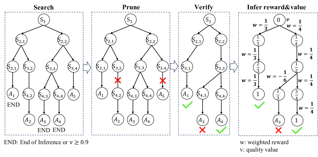<details> <summary>x5.png Details</summary>  ### Visual Description ## Diagram: Four-Stage Search and Inference Process ### Overview The image displays a four-panel technical diagram illustrating a sequential algorithmic process for search, pruning, verification, and reward/value inference. The process is depicted as a directed tree structure that evolves through four distinct stages, labeled from left to right: **Search**, **Prune**, **Verify**, and **Infer reward & value**. The diagram uses nodes (circles) representing states (labeled `S`) and actions (labeled `A`), connected by directional arrows. The final panel introduces numerical weights (`w`) and values (`v`). A legend and a definition are provided at the bottom. ### Components/Axes * **Panel Structure:** Four dashed rectangular boxes arranged horizontally, each with a bold title at the top center. * **Node Types:** * **State Nodes:** Labeled with `S` followed by subscripts (e.g., `S₁`, `S₂,₁`, `S₃,₂`). * **Action Nodes:** Labeled with `A` followed by subscripts (e.g., `A₁`, `A₂`). * **Flow Indicators:** Solid black arrows connect parent nodes to child nodes, indicating the direction of the process flow. * **Status Indicators:** * **Red Cross (X):** Appears in the "Prune" and "Verify" panels, indicating a node or path that is removed or invalid. * **Green Checkmark (✓):** Appears in the "Verify" and "Infer reward & value" panels, indicating a node or path that is verified or valid. * **Legend (Bottom Right of "Infer reward & value" panel):** * `w: weighted reward` * `v: quality value` * **Definition (Bottom Left, below all panels):** * `END: End of Inference or v ≥ 0.9` ### Detailed Analysis #### **Panel 1: Search** * **Structure:** A complete search tree starting from a root node `S₁`. * **Level 1:** `S₁` branches into two nodes: `S₂,₁` (left) and `S₂,₂` (right). * **Level 2:** * `S₂,₁` branches into `S₃,₁` and `S₃,₂`. * `S₂,₂` branches into `S₃,₃` and `S₃,₄`. * **Level 3 (Actions & Termination):** * `S₃,₁` leads to action node `A₁`, which is marked `END`. * `S₃,₂` leads to state node `S₄,₂`, which leads to action node `A₂`, marked `END`. * `S₃,₃` branches into `S₄,₃` and `S₄,₄`. * `S₃,₄` leads to action node `A₅`. * **Level 4:** * `S₄,₃` leads to action node `A₃`, marked `END`. * `S₄,₄` leads to action node `A₄`, marked `END`. #### **Panel 2: Prune** * **Structure:** The same tree structure as the "Search" panel, but with two nodes marked for removal. * **Pruned Nodes (marked with a red X):** * The path from `S₃,₂` to `S₄,₂` is crossed out. * The node `S₃,₄` and its subsequent path to `A₅` are crossed out. * **Remaining Active Paths:** The tree is reduced to two main branches originating from `S₁`: 1. `S₁` -> `S₂,₁` -> `S₃,₁` -> `A₁` 2. `S₁` -> `S₂,₂` -> `S₃,₃` -> (`S₄,₃` -> `A₃`) and (`S₄,₄` -> `A₄`) #### **Panel 3: Verify** * **Structure:** The pruned tree from the previous panel, now with verification status applied to the terminal action nodes. * **Verification Outcomes:** * `A₁` (from the left branch) has a **green checkmark (✓)**. * `A₃` (from the right branch, left sub-branch) has a **red cross (X)**. * `A₄` (from the right branch, right sub-branch) has a **green checkmark (✓)**. * **Implication:** Only the paths leading to `A₁` and `A₄` are considered valid after verification. #### **Panel 4: Infer reward & value** * **Structure:** The verified tree structure, now annotated with numerical values for `w` (weighted reward) and `v` (quality value). The legend defining these terms is located in the bottom-right corner of this panel. * **Root Node (`S₁`):** Contains the value `0` and is labeled with `v`. * **Value Propagation (from leaves to root):** * **Left Branch (to `A₁`):** * Edge from `S₁` to `S₂,₁`: `w = 1/3` * Edge from `S₂,₁` to `S₃,₁`: `w = 1/3` * Edge from `S₃,₁` to `A₁`: `w = 1/3` * Node `A₁` contains the value `1` and has a **green checkmark**. * **Right Branch (to `A₃` and `A₄`):** * Edge from `S₁` to `S₂,₂`: `w = 1/4` * Edge from `S₂,₂` to `S₃,₃`: `w = 1/4` * **Sub-branch to `A₃` (Invalid):** * Edge from `S₃,₃` to `S₄,₃`: `w = -1/6` * Edge from `S₄,₃` to `A₃`: `w = 1/4` * Node `A₃` contains the value `1` and has a **red cross**. * **Sub-branch to `A₄` (Valid):** * Edge from `S₃,₃` to `S₄,₄`: `w = 1/4` * Edge from `S₄,₄` to `A₄`: `w = 1/4` * Node `A₄` contains the value `1` and has a **green checkmark**. * **Intermediate Node Values (Inferred):** * Node `S₂,₁`: Contains `1/3`. * Node `S₃,₁`: Contains `2/3`. * Node `S₂,₂`: Contains `1/4`. * Node `S₃,₃`: Contains `1/2`. * Node `S₄,₃`: Contains `1/3`. * Node `S₄,₄`: Contains `3/4`. ### Key Observations 1. **Process Flow:** The diagram clearly shows a sequential pipeline: exhaustive search -> selective pruning -> validation -> numerical value inference. 2. **Pruning Logic:** The "Prune" stage removes specific branches (`S₃,₂` and `S₃,₄`), reducing the search space before verification. 3. **Verification Outcome:** The "Verify" stage acts as a filter, marking some terminal actions (`A₃`) as invalid despite them being part of the pruned tree. 4. **Value Calculation:** The final stage performs a bottom-up calculation of weighted rewards (`w`). The root node's value (`0`) appears to be an initial state, with values propagating upward from the terminal actions (all set to `1`). 5. **Weight Assignment:** Weights (`w`) are assigned to edges. The left branch uses a consistent weight of `1/3`. The right branch uses `1/4` for most edges, but a negative weight (`-1/6`) is applied to the edge leading to the invalid sub-branch (`S₄,₃`), which likely influences the final verification outcome. 6. **Spatial Layout:** The legend is positioned in the bottom-right of the final panel. The definition for `END` is placed globally at the bottom-left, applying to all panels. ### Interpretation This diagram models a **guided search and evaluation algorithm**, likely for decision-making, planning, or reinforcement learning. The process demonstrates how an initial broad search ("Search") is refined through pruning suboptimal or unpromising paths ("Prune"), followed by a validation step ("Verify") that may further eliminate paths based on a quality criterion. The final stage ("Infer reward & value") quantifies the outcome by propagating weighted rewards back through the verified tree structure. The key insight is the interplay between structural pruning and value-based verification. A path can survive pruning but still fail verification (e.g., the branch to `A₃`). The negative weight (`w = -1/6`) on the edge to `S₄,₃` suggests that the algorithm can assign penalties to certain transitions, which may contribute to the invalidation of that path during verification. The consistent use of fractions for weights implies a normalized or probabilistic framework for reward calculation. The condition `v ≥ 0.9` for an "END" state indicates a high-quality threshold for autonomous termination of the inference process. Overall, the diagram illustrates a method for efficiently navigating a decision tree by combining structural reduction with quantitative evaluation. </details> Figure 4: Detailed process of new sample data generation for the self-training framework. ### Appendix D Model Comparison ReST-MCTS ∗ vs. AlphaLLM. As an approach that aims to enhance LLM inference, AlphaLLM [61] utilizes a tailored MCTS algorithm and critic models to provide precise feedback. Even though AlphaLLM also adopts MCTS and critic models for self-improvement, their approach is different from ours in various crucial aspects, as elaborated below. (1) Design of MCTS algorithm. For the level of search, AlphaLLM’s $η$ MCTS considers options as action, with termination signals delivered by a termination function $β$ . In contrast, we use reasoning steps as action, which is achieved through tailored prompt design. Concerning critic models, we use a single value model to provide evaluation for intermediate nodes. The model is trained to predict specially designed quality values that reflect completeness and correctness of partial solutions, rather than estimating the conventional definition of value function in RL. In addition, we also incorporate self-critic mechanisms into the tree search algorithm to provide insights for the policy (Appendix C.1), which AlphaLLM does not adopt. (2) Definition of reward/value. Our definition of weighted reward and quality value is novel, leading to significant differences between our method and AlphaLLM across various processes such as critic model training, data synthesizing, and data filtration. Since our design of quality value involves information on process reward and reasoning distance, our value model trained on this target can naturally provide sufficient feedback during the search, with no need for implementing other critic models mentioned by AlphaLLM. (3) Self-Training algorithm. Although AlphaLLM also includes iterative self-training, the implementation method varies greatly. Most importantly, their critical model is static throughout the iterations, which means they focus more on the improvement of policy. In comparison, we also consider the impacts of self-training on the critic value model. As demonstrated in Algorithm 1, we calculate process rewards and quality values according to the final search tree of questions within each iteration, which are then used as new training data for the value model. ### Appendix E Experimental Details #### E.1 Training and Evaluation of Initial Value Model Initialization of Value Model. We split $D_V_0$ and use the train set to finetune ChatGLM3-6B and Mistral-7B to predict the value of partial solutions. We simply add a linear layer to the model to directly transform probabilities to a scalar value. Moreover, we use the AdamW optimizer [62] and MSE loss in Eq. (39) to optimize, eventually obtaining an initial value model $V_θ$ that can evaluate the correctness and completeness of step-by-step solutions. Note that the learning rate is set to 1e-6 in this process. The MSE training loss is shown below: $$ L_MSE=E_(q,p,v)∼ D_{V_0}|V_θ(p|q)-v|^2. \tag{39} $$ Evaluation of Value Model. We use the test set containing 14k data samples to evaluate the value model with an absolute tolerance of $0.1$ : $$ Accuracy=\frac{1}{t}Σ_i=1^t I(|clip(V_θ (p_i|q_i),0,1)-v_i^*|<0.1) \tag{40} $$ where $t$ is the number of test data samples, $q_i$ is the question of sample $i$ , $p_i$ is the partial solution of sample $i$ and $v_i^*$ is the target value of sample $i$ . Our initial value model achieves an accuracy of 69.3%, which means it is reliable in most situations. We also conducted a study to measure the value model’s performance on science benchmark SciBench [34] compared to outcome-supervised reward models and self-critic methods in Table 7. #### E.2 Benchmark Setup To compare the performance of different search methods, we construct a standardized benchmark test that can be generally used on labeled science or math datasets like MATH, SciBench, and SciEval. Aside from the ReST-MCTS ∗, we incorporate two other baselines: chain-of-thought (CoT) and tree-of-thought (ToT). For each method, specialized prompts $P$ are designed to execute the search process. Besides, an inference model $π$ and value model $V$ are deployed to provide deduction and feedback. Concerning the CoT baseline, we use Self-Consistency to calculate accuracy. For the ToT baseline, we use a simple greedy depth-first-search (DFS) algorithm with node values assigned by the value model. The algorithm stops exploitation when a max depth of $10$ is reached and ends when a node value exceeds the threshold $0.9$ . For ReST-MCTS ∗, self-critic is used and the ending threshold is also set to $0.9$ . The rollout step limit $m$ is set to $2$ , $α$ is set to $0.5$ , and the number of iterations $T$ is set to $50$ by default. Moreover, both tree search algorithms use $b=3$ by default, where $b$ is the number of samples generated in the expansion process as mentioned in the former sections. After the search process, the policy is prompted to extract the final answer based on the obtained solution, which is then compared with the ground truth to determine correctness. The results of these methods on benchmarks are illustrated in Section 4.3. #### E.3 Baselines of Search Verification The basic settings of relevant verification baselines are illustrated as follows: - ORM + Best-of-N (BoN) For simplicity, we employ the ORM used by [10], which is trained on SciInstruct. For each question, we sample $N$ solutions and select the solution with the highest ORM score as output. $N$ is used to control token usage. - ReST-MCTS ∗ Implementation of ReST-MCTS ∗, using the value model $V_θ$ as PRM to guide MCTS ∗. The variable controlling token usage is the iteration number $T$ and branch parameter $b$ . - Self-Consistency $N$ solutions are generated for each question using a simple CoT prompt. Their final answers are then extracted and classified, with the most frequently occurring answer selected as the final output. $N$ is used to control token usage. - PRM + Best-of-N (BoN) With value model $V_θ$ used as PRM, we perform DFS-based tree search. Every selected solution $s$ is evaluated by a PRM score $r_PRM=Π_i=1^Kv_i$ . The one with the highest PRM score among all $N$ solutions is regarded as the final output. Under this setting, $b$ is set to $3$ , while $N$ is used to control token usage. Table 6: The average running time of different algorithms (under our basic experiment settings) on a single question. | Method | CoT + SC | ORM + BoN | PRM + BoN | MCTS ∗ | | --- | --- | --- | --- | --- | | Running time (s) | 41 | 43 | 73 | 108 | | MATH | 37.0 | 33.5 | 34.5 | 41.5 | As shown in Figure 2, we have compared the number of tokens consumed by each algorithm to achieve certain accuracy on MATH and SciBench. Results reveal that to reach a certain expected accuracy, MCTS ∗ basically requires fewer tokens than other algorithms like SC and ORM + BoN. This means that based on the same expected standards, MCTS ∗ outperforms other algorithms while maintaining a reasonable computation cost. As for the actual running time, we have recorded the average running time of different algorithms (under our basic experiment settings) on a single question, as shown in Table 6. We see that MCTS ∗ spends more time on exploration and simulation than other simple algorithms. However, since our method adopts a different design of value, it does not require massive Monte Carlo estimations. This reduces the running time of our algorithm and limits the time consumption to a reasonable range. Notice that MCTS ∗ can achieve high accuracy that other algorithms can never attain even at unlimited cost, we believe this extra time is fairly acceptable. Table 7: Accuracy of different reward/value models on the questions selected from SciBench, they all use MCTS ∗ as search policy. 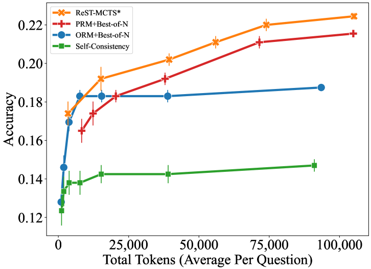| Dataset | Models | ORM | PRM | Self-Rewarding | ReST-MCTS ∗ (Value) | | --- | --- | --- | --- | --- | --- | | SciBench | GLM4 | 20.2 | 22.0 | 20.2 | 22.9 | | GPT-3.5-turbo | 12.8 | 17.4 | 13.7 | 20.2 | | <details> <summary>x6.png Details</summary>  ### Visual Description \n ## Line Chart: Accuracy vs. Total Tokens (Average Per Question) ### Overview This image is a line chart comparing the performance (accuracy) of four different computational methods or models as a function of the average number of tokens used per question. The chart demonstrates how accuracy scales with increased computational effort (token usage) for each method. ### Components/Axes * **Chart Type:** Line chart with error bars. * **X-Axis:** * **Label:** "Total Tokens (Average Per Question)" * **Scale:** Linear, ranging from 0 to 100,000. * **Major Tick Marks:** 0, 25,000, 50,000, 75,000, 100,000. * **Y-Axis:** * **Label:** "Accuracy" * **Scale:** Linear, ranging from approximately 0.12 to 0.22. * **Major Tick Marks:** 0.12, 0.14, 0.16, 0.18, 0.20, 0.22. * **Legend:** Located in the top-left corner of the plot area. It defines four data series: 1. **ReST-MCTS\***: Orange line with star (`*`) markers. 2. **PRM+Best-of-N**: Red line with plus (`+`) markers. 3. **ORM+Best-of-N**: Blue line with circle (`●`) markers. 4. **Self-Consistency**: Green line with square (`■`) markers. ### Detailed Analysis The chart plots four distinct data series. Each point includes vertical error bars, indicating variability or confidence intervals around the accuracy measurement. **1. ReST-MCTS\* (Orange, Star Markers)** * **Trend:** Shows a strong, consistent upward trend. Accuracy increases steeply at low token counts and continues to rise steadily across the entire range. * **Approximate Data Points:** * ~0 tokens: Accuracy ~0.125 * ~5,000 tokens: Accuracy ~0.175 * ~15,000 tokens: Accuracy ~0.192 * ~40,000 tokens: Accuracy ~0.202 * ~60,000 tokens: Accuracy ~0.210 * ~75,000 tokens: Accuracy ~0.220 * ~105,000 tokens: Accuracy ~0.225 (highest point on the chart) **2. PRM+Best-of-N (Red, Plus Markers)** * **Trend:** Also shows a strong upward trend, closely following but slightly below the ReST-MCTS* line. The rate of improvement is similar. * **Approximate Data Points:** * ~5,000 tokens: Accuracy ~0.165 * ~10,000 tokens: Accuracy ~0.175 * ~20,000 tokens: Accuracy ~0.183 * ~40,000 tokens: Accuracy ~0.192 * ~75,000 tokens: Accuracy ~0.210 * ~105,000 tokens: Accuracy ~0.215 **3. ORM+Best-of-N (Blue, Circle Markers)** * **Trend:** Shows a rapid initial increase in accuracy at very low token counts, then plateaus sharply. After approximately 10,000 tokens, the accuracy remains nearly flat, showing minimal gain from additional tokens. * **Approximate Data Points:** * ~0 tokens: Accuracy ~0.125 * ~2,500 tokens: Accuracy ~0.145 * ~5,000 tokens: Accuracy ~0.170 * ~10,000 tokens: Accuracy ~0.182 (plateau begins) * ~15,000 tokens: Accuracy ~0.182 * ~40,000 tokens: Accuracy ~0.182 * ~90,000 tokens: Accuracy ~0.188 **4. Self-Consistency (Green, Square Markers)** * **Trend:** Shows a modest, gradual upward trend. It starts at a similar accuracy to the others at 0 tokens but improves at a much slower rate. It remains the lowest-performing method across the entire range. * **Approximate Data Points:** * ~0 tokens: Accuracy ~0.125 * ~2,500 tokens: Accuracy ~0.135 * ~5,000 tokens: Accuracy ~0.138 * ~15,000 tokens: Accuracy ~0.142 * ~40,000 tokens: Accuracy ~0.142 * ~90,000 tokens: Accuracy ~0.148 ### Key Observations 1. **Performance Hierarchy:** There is a clear and consistent performance hierarchy across most of the token range: ReST-MCTS* > PRM+Best-of-N > ORM+Best-of-N > Self-Consistency. 2. **Scaling Behavior:** ReST-MCTS* and PRM+Best-of-N demonstrate favorable scaling properties, with accuracy continuing to improve significantly as more tokens are allocated. ORM+Best-of-N exhibits a "diminishing returns" pattern, saturating early. Self-Consistency scales poorly. 3. **Initial Convergence:** All methods start at a very similar accuracy level (~0.125) with near-zero token usage, suggesting a common baseline. 4. **Error Bars:** The error bars appear relatively consistent in size for each series, suggesting stable variance in the measurements. They do not overlap between the top two methods (ReST-MCTS* and PRM+Best-of-N) and the bottom two (ORM+Best-of-N and Self-Consistency) at higher token counts, indicating statistically distinct performance. ### Interpretation This chart likely comes from research on reasoning or problem-solving with large language models, where "tokens" represent computational effort (e.g., steps in a reasoning chain, samples generated). * **What the data suggests:** The data demonstrates that the **ReST-MCTS\*** method is the most effective and efficient at converting increased computational budget (tokens) into higher accuracy. It outperforms the other methods, especially at higher token budgets. **PRM+Best-of-N** is a close second. * **Relationship between elements:** The chart directly compares algorithmic strategies. The stark difference between the plateau of **ORM+Best-of-N** and the continued rise of **ReST-MCTS\*** suggests a fundamental advantage in the latter's approach to utilizing additional computation. **Self-Consistency**, while improving, is a less token-efficient strategy. * **Notable implications:** The results argue for the use of methods like ReST-MCTS* when high accuracy is critical and computational resources (token budget) are available. The early plateau of ORM+Best-of-N indicates it may be a good choice for low-latency applications where token usage must be minimized, but it is not suitable for pushing accuracy to its limits. The chart provides a clear empirical basis for selecting a method based on the available token budget and desired accuracy target. </details> Figure 5: Accuracy of different methods on SciBench with varied total token usage per question. Both the completion token and prompt token are included. #### E.4 Value Model of ReST-MCTS ∗ on SciBench We employ the reward model obtained by [10] (which is used as a classifier for SciGLM) as the ORM and our fine-grained value model as PRM to provide the outcome reward and step-wise value respectively. We also include the Self-Rewarding method, where the policy model itself is instructed to provide step-wise value. For all methods, the number of samples for each step is set to $3$ . Using this setting, we record the model accuracy of GLM4 and GPT-3.5-turbo on the selected questions, which are as shown in Table 7. Results indicate that compared to ORM and Self-Rewarding, PRM-based methods exhibit higher accuracy. This confirms the effectiveness of our value model. In addition, Figure 5 concerns the total consumption of the token budget, including all prompt tokens and completion tokens. However, we still have to note that the total token usage (especially prompt tokens) of the ReST-MCTS ∗ increases rapidly as hyper-parameters $b$ and $T$ rise. Table 8: Overall performance comparison with representative models on SciEval. | Models | Method | Part I | Part II | Part III | Part IV | Ave. | | --- | --- | --- | --- | --- | --- | --- | | GLM4 | CoT | 52.50 | 85.83 | 80.83 | 78.11 | 74.32 | | ToT | 60.83 | 87.77 | 84.16 | 79.77 | 78.13 | | | ReST-MCTS ∗ | 69.16 | 88.05 | 83.33 | 78.94 | 79.87 | | | GPT-3.5-Turbo | CoT | 28.88 | 78.61 | 70.00 | 71.46 | 62.24 | | ToT | 32.50 | 76.11 | 68.05 | 67.59 | 61.06 | | | ReST-MCTS ∗ | 29.72 | 78.88 | 69.72 | 70.91 | 62.31 | | #### E.5 ReST-MCTS ∗ on SciEval SciEval. Similar to SciBench, we perform benchmark tests on SciEval. Results are shown in Table 8. For both GLM4 and GPT-3.5-turbo, ReST-MCTS ∗ again outperforms other baselines in overall accuracy, with an accuracy of $79.87\$ and $62.31\$ respectively. However, we notice that though tree-search-based methods demonstrate an advantage on average, they fail to improve the performance of the CoT baseline on some parts of SciEval. We examine the data distribution and discover that these parts are basically all single-choice questions. As they are less difficult compared to other types of questions, the Self-Consistency CoT approach may already be competent. Besides, these questions often require few reasoning steps, which may be the main reason why tree search methods do not perform as well as expected. ### Appendix F Prompt and Instruction Examples We present some instruction examples used in ReST-MCTS ∗ and self-training process in this section, including: - Inference instruction This instruction is used in tree search for the policy to generate new steps based on previous self-critic information. - Self-critic instruction Used for generating the EoI signal or advice for further search. - LLM verify instruction This instruction is employed in the data generation process of self-training when an answer needs verification by LLM (GPT-4 for our case). 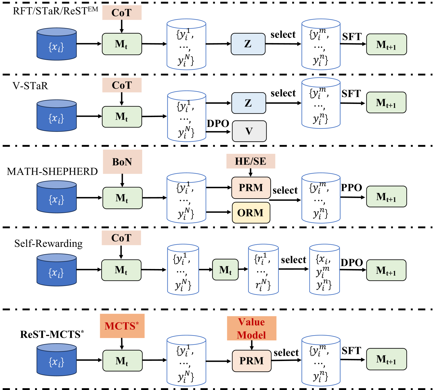<details> <summary>x7.png Details</summary>  ### Visual Description ## [Diagram Type]: Machine Learning Training Pipeline Comparison ### Overview The image is a technical diagram illustrating five distinct iterative training pipelines for machine learning models, specifically focusing on methods for improving model performance through self-generated data and reinforcement learning. The diagram is organized vertically into five horizontal sections, each separated by a thick dashed black line, representing a different method or family of methods. Each pipeline follows a similar left-to-right flow: starting with an input dataset, processing through a model, generating outputs, applying a selection or reward mechanism, and finally updating the model. ### Components/Axes The diagram is not a chart with axes but a process flow diagram. The key components are: * **Input Data**: Represented by a blue cylinder labeled `{x_i}`. * **Models**: Represented by green rounded rectangles labeled `M_t` (current model) and `M_{t+1}` (updated model). * **Generated Outputs**: Represented by white cylinders containing sets of outputs, e.g., `{y_i^1, ..., y_i^N}`. * **Selection/Reward Mechanisms**: Represented by various colored boxes (light blue, light orange, light yellow) with labels like `Z`, `V`, `PRM`, `ORM`. * **Training Methods**: Labeled on the arrows between components, such as `SFT`, `DPO`, `PPO`. * **Prompting/Generation Strategies**: Labeled in light orange boxes above the first model, such as `CoT`, `BoN`, `MCTS*`. ### Detailed Analysis The diagram details five pipelines: **1. RFT/STaR/ReSTEM** * **Flow**: `{x_i}` → `M_t` (with `CoT` prompting) → `{y_i^1, ..., y_i^N}` → `Z` (selection) → `{y_i^m, ..., y_i^n}` → `SFT` → `M_{t+1}`. * **Key Components**: Uses Chain-of-Thought (`CoT`) prompting. A selection module `Z` filters the generated outputs before Supervised Fine-Tuning (`SFT`). **2. V-STaR** * **Flow**: `{x_i}` → `M_t` (with `CoT` prompting) → `{y_i^1, ..., y_i^N}` → splits into two paths: * Path 1: → `Z` (selection) → `{y_i^m, ..., y_i^n}` → `SFT` → `M_{t+1}`. * Path 2: → `DPO` → `V` (a value or verifier model). * **Key Components**: Similar to the first pipeline but incorporates a separate `DPO` (Direct Preference Optimization) path to train a verifier model `V`. **3. MATH-SHEPHERD** * **Flow**: `{x_i}` → `M_t` (with `BoN` prompting) → `{y_i^1, ..., y_i^N}` → splits into two paths: * Path 1: → `PRM` (Process Reward Model, with `HE/SE` input) → `select` → `{y_i^m, ..., y_i^n}` → `PPO` → `M_{t+1}`. * Path 2: → `ORM` (Outcome Reward Model). * **Key Components**: Uses Best-of-N (`BoN`) prompting. Employs both a Process Reward Model (`PRM`) and an Outcome Reward Model (`ORM`) for selection. The final training uses Proximal Policy Optimization (`PPO`). `HE/SE` likely refers to Heuristic Search or similar. **4. Self-Rewarding** * **Flow**: `{x_i}` → `M_t` (with `CoT` prompting) → `{y_i^1, ..., y_i^N}` → `M_t` (the same model acts as a rater) → `{r_i^1, ..., r_i^N}` (rewards) → `select` → `{x_i, y_i^m, y_i^n}` → `DPO` → `M_{t+1}`. * **Key Components**: The model `M_t` is used twice: first to generate outputs, then to generate rewards (`r_i`) for those outputs. Selection is based on these self-generated rewards, and training is done via `DPO`. **5. ReST-MCTS*** * **Flow**: `{x_i}` → `M_t` (with `MCTS*` prompting) → `{y_i^1, ..., y_i^N}` → `PRM` (with `Value Model` input) → `select` → `{y_i^m, ..., y_i^n}` → `SFT` → `M_{t+1}`. * **Key Components**: Uses Monte Carlo Tree Search (`MCTS*`) for generation. A `PRM` is guided by a separate `Value Model` for selection, followed by `SFT`. ### Key Observations * **Common Pattern**: All pipelines share a core loop: Generate → Select/Score → Train. They are all methods for **iterative self-improvement** or **reinforcement learning from self-generated data**. * **Variations in Generation**: Prompting strategies vary: `CoT` (3 pipelines), `BoN` (1), `MCTS*` (1). * **Variations in Selection/Reward**: Selection mechanisms range from a simple selector `Z`, to dedicated reward models (`PRM`, `ORM`), to the model rating its own outputs. * **Variations in Training**: Final training steps include `SFT` (3 pipelines), `DPO` (2 pipelines), and `PPO` (1 pipeline). * **Spatial Layout**: The legend/labels for each pipeline are consistently placed to the left of the flow. The prompting strategy is always in a light orange box above the first model (`M_t`). Selection/reward model boxes are placed centrally between the generation and training stages. ### Interpretation This diagram provides a comparative taxonomy of modern techniques for training large language models (LLMs) to improve their reasoning or problem-solving abilities, particularly in domains like mathematics (hinted at by `MATH-SHEPHERD`). The overarching theme is **bootstrapping**: using the model's own outputs to create training data for its next iteration. * **What it demonstrates**: It shows the evolution from simpler methods (like RFT/STaR which use basic selection) to more complex ones that incorporate explicit reward models (`PRM/ORM`) or advanced search algorithms (`MCTS*`). The "Self-Rewarding" pipeline is notable for its simplicity, using the model as its own evaluator. * **Relationships**: The pipelines are not mutually exclusive; they represent a spectrum of approaches. For instance, `V-STaR` can be seen as an extension of the basic `STaR` method by adding a verifier. `MATH-SHEPHERD` and `ReST-MCTS*` represent more sophisticated, resource-intensive approaches using separate reward/value models. * **Notable Trends**: There is a clear trend towards using more sophisticated **process-based supervision** (`PRM`) over simple outcome-based selection (`Z` or `ORM`), as process models can provide finer-grained feedback. The use of `DPO` as an alternative to `PPO` for the final training step is also a notable modern trend, as it can be more stable and efficient. * **Underlying Message**: The diagram argues that the key to iterative improvement lies in the **quality of the selection/reward mechanism**. The choice of generation strategy (`CoT` vs. `MCTS*`) and training algorithm (`SFT` vs. `DPO` vs. `PPO`) are important, but the core innovation in these methods is how they filter or score the model's own generations to create high-quality training data. </details> Figure 6: Comparison between existing self-training methods with our proposed ReST-MCTS ∗. This is an example of inference instruction. Instruction: Given a science or math problem, a corresponding solution that may be incomplete as well as some advice on solving this problem, your task is to generate a new solution step based on the advice and existing steps. Problem: Let $a$ and $b$ satisfy $ab=7$ and $a+b=5$ . What is the value of $a^2+b^2$ ?. Solution: Step 1: From $a+b=5$ , we can know that $(a+b)^2=25$ . Step 2: Thus, $a^2+2ab+b^2=25$ . Advice: From step 2 we know the value of $a^2+2ab+b^2$ . Since we also know the value of $ab$ , we can derive $a^2+b^2$ . Policy Output: Since $a^2+2ab+b^2=25$ and $ab=7$ , we derive $a^2+b^2=(a^2+2ab+b^2)-2ab=25-14=11$ . This is an example of self-critic instruction. Instruction: Given a science or math problem and a corresponding solution that may be incomplete, your task is to judge whether the solution has already reached a final answer or conclusion for the problem. If the solution has already reached a final answer or conclusion, you should directly output "Final answer reached". Otherwise, you should give some advice on how to solve the problem based on current steps or what to consider next. Problem: Let $a$ and $b$ satisfy $ab=7$ and $a+b=5$ . What is the value of $a^2+b^2$ ?. Solution: Step 1: From $a+b=5$ , we can know that $(a+b)^2=25$ . Step 2: Thus, $a^2+2ab+b^2=25$ . Policy Output: The solution has not reached a final answer. Advice: From step 2 we know the value of $a^2+2ab+b^2$ . Since we also know the value of $ab$ , we can derive $a^2+b^2$ . This is an example of LLM verify instruction. Instruction: Given a science or math problem, a corresponding step-by-step solution, and the true answer of the problem, your task is to verify the answer obtained in the solution with the real answer. If the answer obtained in the solution is equivalent to the real one, output ’1’, otherwise output ’0’. Problem: Let $a$ and $b$ satisfy $ab=7$ and $a+b=5$ . What is the value of $a^2+b^2$ ?. Solution: Step 1: From $a+b=5$ , we can know that $(a+b)^2=25$ . Step 2: Thus, $a^2+2ab+b^2=25$ . Step 3: Since $ab=7$ , we can derive that $a^2+b^2=(a^2+2ab+b^2)-2ab=25-14=11$ . So the answer is $11$ . Real Answer: The value of $a^2+b^2$ is $11$ . LLM Output: $1$ ### Appendix G Further Preliminaries of MCTS and LLM Reasoning with MCTS #### G.1 Monte Carlo Tree Search (MCTS) MCTS [63] is a search algorithm for optimal decision-making in large and complex combinatorial spaces. This algorithm represents search spaces as search trees and works on the principle of the best-first search based on the evaluations of stochastic simulations. This technique has been widely employed in multiple gaming scenarios and achieved tremendous success, such as AlphaGo and AlphaZero [64] for computer Go Game. The basic MCTS algorithm involves iteratively search process with four steps for building a search tree: (1) Selection. The agent, starting from an empty tree’s root node, traverses the search tree’s visited nodes and selects the next node according to the given selection strategy until the scalable node or leaf node is reached. (2) Expansion. If this algorithm arrives at an expandable node, it expands the search tree by selecting an unvisited child node. (3) Simulation. After finishing the expansion, if the current node is in a non-terminal state, the algorithm will conduct one or multiple independent simulations from the current node until it reaches the terminal state. In this process, the actions are chosen at random. (4) Backpropagation. The node statistics on the path from the current node to the root are updated based on the search results. Note that the scores assessed are based on the termination state achieved. To trade off the less tested paths with the best strategy identified so far, MCTS maintains a proper balance between exploration and exploitation by maximizing the Upper Confidence Bounds for Trees (UCT) when a child node $k$ is selected as follows, $UCT=\overline{X}_k+2C_p√{\frac{2\ln n}{n_k}}$ : where the first term, $\overline{X}_k$ , is the average reward form arm $k$ and this term encourages the exploitation of higher-reward choices. It is generally understood that $\overline{X}_k$ to be within [0, 1]. In the second exploration term, $C_p>0$ is a constant to satisfy the Hoeffding inequality with rewards in the range of [0, 1] [26]. $n$ is the number of times the current node has been visited and $n_k$ is the number of times child $k$ has been visited. Generally, $n_k=0$ produces a UCT value of $∞$ , so that all children of a node have a non-zero probability and are considered. #### G.2 LLM Reasoning with Monte Carlo Tree Search LLMs have been invented, used in the past for autoregressive text generation, and are now very great at reasoning. Reasoning algorithms include prompt-based chain-of-thought (CoT) [22], planning-based represented by tree-of-thought (ToT) [24], which successfully achieved the LLMs’ reasoning performance improvement. ToT combines the power of tree search (e.g., depth/breadth-first search) as an algorithm and LLMs’ power as a heuristic to tradeoff evaluation and generation. Reasoning via Planning (RAP) [59] with Monto Carlo Tree Search (MCTS) performs reasoning exploration and obtains reward reasoning paths. Recent studies [60] present that Monte Carlo Tree Search (MCTS) agents benefit from task-specific extension and expansion of the research tree. Specifically, the MCTS agents provide appropriate selection strategies for the state of the visit to guide the upcoming search based on the evaluation results (e.g., rewards and number of times the node has been visited) produced by the rollout and backpropagation process. Its mechanism coordinates exploration and thought exploitation within search space, which is superior to traditional depth-first search (DFS) or breadth-first search (BFS) algorithms based on the Tree of Thought (ToT). Building on MCTS, some studies have also explored the ability of the reasoning agent to provide search guidance. In catalyst design, [65] proposed Monte Carlo Thought Search, using LLM for complex scientific reasoning queries. [59] presents Reasoning via Planning (RAP), which adopts MCTS as a planning algorithm and repurposes the LLM as both a world model and a reasoning agent. Others like [66] experiment using the value function, a byproduct of the Proximal Policy Optimization (PPO) process, to guide the token-level decoding based on MCTS. In general, these approaches improve LLM’s reasoning ability, whereas their performance on some challenging science tasks remains unsatisfying. In addition, this series of methods differs from our contribution, where we propose a value model approach as reward functions for optimizing the reasoning path and improving model output. ### Appendix H Limitations In this section, we discuss some limitations of the ReST-MCTS ∗. Generalization to other tasks, especially those without labels. Similar to many existing self-training works, ReST-MCTS ∗ also relies on ground-truth oracle labels in a supervised dataset to filter the responses in the first place; in the future, we need to show ReST-MCTS ∗ can generalize to other reasoning tasks outside of math (like coding, agent, conversation, etc); in addition, for those very complicated tasks that require multistep planning and reasoning (like implementing the whole software like SWE-Agent), which does not have ground-truth answers, we need to propose a better way to collect reward feedback (from few human labeling and symbolic execution or solver), and train a generalizable reward model that can work and help for a wider range of tasks. Scale and diversity of proposed value model. Although we trained a value model based on Mistral-7B: MetaMATH that performs better than the most advanced value model MATH-SHEPHERD, a larger scale value model backbone is still needed for better PRM training. In addition, the initial training set of the training proposal PRM was generated by SciGLM, a model that focuses on mathematical and scientific reasoning tasks but still lacks generality. While the current PRM achieves the best results on multiple mathematical and scientific reasoning tasks, such as MATH and SciBench, it’s worth exploring more diverse training sets to expand into various fields in the future, such as code generation and agent planning. Self-training data filtering techniques. As we mentioned in Section 1, the quality of reasoning trajectory affects the effectiveness of self-training, and generating a high-quality training set plays an important role. Therefore, we train the iterative process reward model to guide the tree search direction to obtain high-quality trajectories. On the other hand, since well-trained value models can help filter out the top-k generated trajectories with the highest process values, we also expect that a stronger and larger LLM model as the backbone of the value model might help to gain more. ### Appendix I Broader Impact ReST-MCTS ∗ aims to introduce a general self-training approach that uses MCTS ∗ to automatically label and generate process rewards, which will help generate high-quality datasets and improve the reasoning capabilities of LLMs. Fine-tuning a variety of LLMs on synthesized high-quality datasets can directly improve the performance of value models and generators and help to avoid the cost of manually generating process rewards during the training process reward model. The disadvantage is that a single reward model cannot be scaled to multiple domains, and we can solve this problem by training various reward models together on various reasoning domains. We believe that on the whole, the advantages outweigh the disadvantages. ### Appendix J Reproducibility We have made significant efforts to ensure the reproducibility of our all experimental results. The training code, tree search algorithm, and the evaluation details for the ReST-MCTS ∗ are public in our repository. Training. Detailed training information about the value model, self-training backbones, and experimental settings can be found in Section 4.1. Tree Search Algorithm. Regarding the enhanced tree search algorithm MCTS ∗, please refer to the Algorithm 1 and public code. Evaluation. We organized all evaluations, including the iterative self-training and value model, a variety of value models, performance comparison under the same search budget, and different reasoning policies. All details can be found in Section 4.2 for self-improvement evaluation and Section 4.3 for value models and reasoning policies comparison. ### NeurIPS Paper Checklist 1. Claims 1. Question: Do the main claims made in the abstract and introduction accurately reflect the paper’s contributions and scope? 1. Answer: [Yes] 1. Justification: We have provided the main claims of our research in the abstract and introduction. 1. Guidelines: - The answer NA means that the abstract and introduction do not include the claims made in the paper. - The abstract and/or introduction should clearly state the claims made, including the contributions made in the paper and important assumptions and limitations. A No or NA answer to this question will not be perceived well by the reviewers. - The claims made should match theoretical and experimental results, and reflect how much the results can be expected to generalize to other settings. - It is fine to include aspirational goals as motivation as long as it is clear that these goals are not attained by the paper. 1. Limitations 1. Question: Does the paper discuss the limitations of the work performed by the authors? 1. Answer: [Yes] 1. Justification: We have provided the limitations of our research in Section H. 1. Guidelines: - The answer NA means that the paper has no limitation while the answer No means that the paper has limitations, but those are not discussed in the paper. - The authors are encouraged to create a separate "Limitations" section in their paper. - The paper should point out any strong assumptions and how robust the results are to violations of these assumptions (e.g., independence assumptions, noiseless settings, model well-specification, asymptotic approximations only holding locally). The authors should reflect on how these assumptions might be violated in practice and what the implications would be. - The authors should reflect on the scope of the claims made, e.g., if the approach was only tested on a few datasets or with a few runs. In general, empirical results often depend on implicit assumptions, which should be articulated. - The authors should reflect on the factors that influence the performance of the approach. For example, a facial recognition algorithm may perform poorly when image resolution is low or images are taken in low lighting. Or a speech-to-text system might not be used reliably to provide closed captions for online lectures because it fails to handle technical jargon. - The authors should discuss the computational efficiency of the proposed algorithms and how they scale with dataset size. - If applicable, the authors should discuss possible limitations of their approach to address problems of privacy and fairness. - While the authors might fear that complete honesty about limitations might be used by reviewers as grounds for rejection, a worse outcome might be that reviewers discover limitations that aren’t acknowledged in the paper. The authors should use their best judgment and recognize that individual actions in favor of transparency play an important role in developing norms that preserve the integrity of the community. Reviewers will be specifically instructed to not penalize honesty concerning limitations. 1. Theory Assumptions and Proofs 1. Question: For each theoretical result, does the paper provide the full set of assumptions and a complete (and correct) proof? 1. Answer: [Yes] 1. Justification: We have provided the theory assumptions and proofs of our research in Section B.1 and Section B.2. 1. Guidelines: - The answer NA means that the paper does not include theoretical results. - All the theorems, formulas, and proofs in the paper should be numbered and cross-referenced. - All assumptions should be clearly stated or referenced in the statement of any theorems. - The proofs can either appear in the main paper or the supplemental material, but if they appear in the supplemental material, the authors are encouraged to provide a short proof sketch to provide intuition. - Inversely, any informal proof provided in the core of the paper should be complemented by formal proofs provided in appendix or supplemental material. - Theorems and Lemmas that the proof relies upon should be properly referenced. 1. Experimental Result Reproducibility 1. Question: Does the paper fully disclose all the information needed to reproduce the main experimental results of the paper to the extent that it affects the main claims and/or conclusions of the paper (regardless of whether the code and data are provided or not)? 1. Answer: [Yes] 1. Justification: We have provided the experimental result reproducibility of our research in Section J. 1. Guidelines: - The answer NA means that the paper does not include experiments. - If the paper includes experiments, a No answer to this question will not be perceived well by the reviewers: Making the paper reproducible is important, regardless of whether the code and data are provided or not. - If the contribution is a dataset and/or model, the authors should describe the steps taken to make their results reproducible or verifiable. - Depending on the contribution, reproducibility can be accomplished in various ways. For example, if the contribution is a novel architecture, describing the architecture fully might suffice, or if the contribution is a specific model and empirical evaluation, it may be necessary to either make it possible for others to replicate the model with the same dataset, or provide access to the model. In general. releasing code and data is often one good way to accomplish this, but reproducibility can also be provided via detailed instructions for how to replicate the results, access to a hosted model (e.g., in the case of a large language model), releasing of a model checkpoint, or other means that are appropriate to the research performed. - While NeurIPS does not require releasing code, the conference does require all submissions to provide some reasonable avenue for reproducibility, which may depend on the nature of the contribution. For example 1. If the contribution is primarily a new algorithm, the paper should make it clear how to reproduce that algorithm. 1. If the contribution is primarily a new model architecture, the paper should describe the architecture clearly and fully. 1. If the contribution is a new model (e.g., a large language model), then there should either be a way to access this model for reproducing the results or a way to reproduce the model (e.g., with an open-source dataset or instructions for how to construct the dataset). 1. We recognize that reproducibility may be tricky in some cases, in which case authors are welcome to describe the particular way they provide for reproducibility. In the case of closed-source models, it may be that access to the model is limited in some way (e.g., to registered users), but it should be possible for other researchers to have some path to reproducing or verifying the results. 1. Open access to data and code 1. Question: Does the paper provide open access to the data and code, with sufficient instructions to faithfully reproduce the main experimental results, as described in supplemental material? 1. Answer: [Yes] 1. Justification: We have uploaded all codes of our research at https://github.com/THUDM/ReST-MCTS. 1. Guidelines: - The answer NA means that paper does not include experiments requiring code. - Please see the NeurIPS code and data submission guidelines (https://nips.cc/public/guides/CodeSubmissionPolicy) for more details. - While we encourage the release of code and data, we understand that this might not be possible, so “No” is an acceptable answer. Papers cannot be rejected simply for not including code, unless this is central to the contribution (e.g., for a new open-source benchmark). - The instructions should contain the exact command and environment needed to run to reproduce the results. See the NeurIPS code and data submission guidelines (https://nips.cc/public/guides/CodeSubmissionPolicy) for more details. - The authors should provide instructions on data access and preparation, including how to access the raw data, preprocessed data, intermediate data, and generated data, etc. - The authors should provide scripts to reproduce all experimental results for the new proposed method and baselines. If only a subset of experiments are reproducible, they should state which ones are omitted from the script and why. - At submission time, to preserve anonymity, the authors should release anonymized versions (if applicable). - Providing as much information as possible in supplemental material (appended to the paper) is recommended, but including URLs to data and code is permitted. 1. Experimental Setting/Details 1. Question: Does the paper specify all the training and test details (e.g., data splits, hyperparameters, how they were chosen, type of optimizer, etc.) necessary to understand the results? 1. Answer: [Yes] 1. Justification: We have provided the experimental setting and details of our research in Section E.1 and Section E.2. 1. Guidelines: - The answer NA means that the paper does not include experiments. - The experimental setting should be presented in the core of the paper to a level of detail that is necessary to appreciate the results and make sense of them. - The full details can be provided either with the code, in appendix, or as supplemental material. 1. Experiment Statistical Significance 1. Question: Does the paper report error bars suitably and correctly defined or other appropriate information about the statistical significance of the experiments? 1. Answer: [Yes] 1. Justification: We have provided the experimental statistical significance of our research in Figure 2 in Section 4.3. 1. Guidelines: - The answer NA means that the paper does not include experiments. - The authors should answer "Yes" if the results are accompanied by error bars, confidence intervals, or statistical significance tests, at least for the experiments that support the main claims of the paper. - The factors of variability that the error bars are capturing should be clearly stated (for example, train/test split, initialization, random drawing of some parameter, or overall run with given experimental conditions). - The method for calculating the error bars should be explained (closed form formula, call to a library function, bootstrap, etc.) - The assumptions made should be given (e.g., Normally distributed errors). - It should be clear whether the error bar is the standard deviation or the standard error of the mean. - It is OK to report 1-sigma error bars, but one should state it. The authors should preferably report a 2-sigma error bar than state that they have a 96% CI, if the hypothesis of Normality of errors is not verified. - For asymmetric distributions, the authors should be careful not to show in tables or figures symmetric error bars that would yield results that are out of range (e.g. negative error rates). - If error bars are reported in tables or plots, The authors should explain in the text how they were calculated and reference the corresponding figures or tables in the text. 1. Experiments Compute Resources 1. Question: For each experiment, does the paper provide sufficient information on the computer resources (type of compute workers, memory, time of execution) needed to reproduce the experiments? 1. Answer: [Yes] 1. Justification: We have provided the experiments compute resources of our research in Table 2 in Section 4. 1. Guidelines: - The answer NA means that the paper does not include experiments. - The paper should indicate the type of compute workers CPU or GPU, internal cluster, or cloud provider, including relevant memory and storage. - The paper should provide the amount of compute required for each of the individual experimental runs as well as estimate the total compute. - The paper should disclose whether the full research project required more compute than the experiments reported in the paper (e.g., preliminary or failed experiments that didn’t make it into the paper). 1. Code Of Ethics 1. Question: Does the research conducted in the paper conform, in every respect, with the NeurIPS Code of Ethics https://neurips.cc/public/EthicsGuidelines? 1. Answer: [Yes] 1. Justification: We have reviewed the NeurIPS Code of Ethics and make sure to preserve anonymity. Our research is based on open-source models and datasets and we cite all original papers that produced the code package or dataset. There is nothing that violates the NeurIPS Code of Ethics in our work. 1. Guidelines: - The answer NA means that the authors have not reviewed the NeurIPS Code of Ethics. - If the authors answer No, they should explain the special circumstances that require a deviation from the Code of Ethics. - The authors should make sure to preserve anonymity (e.g., if there is a special consideration due to laws or regulations in their jurisdiction). 1. Broader Impacts 1. Question: Does the paper discuss both potential positive societal impacts and negative societal impacts of the work performed? 1. Answer: [Yes] 1. Justification: We have provided the broader impacts of our research in Section I. 1. Guidelines: - The answer NA means that there is no societal impact of the work performed. - If the authors answer NA or No, they should explain why their work has no societal impact or why the paper does not address societal impact. - Examples of negative societal impacts include potential malicious or unintended uses (e.g., disinformation, generating fake profiles, surveillance), fairness considerations (e.g., deployment of technologies that could make decisions that unfairly impact specific groups), privacy considerations, and security considerations. - The conference expects that many papers will be foundational research and not tied to particular applications, let alone deployments. However, if there is a direct path to any negative applications, the authors should point it out. For example, it is legitimate to point out that an improvement in the quality of generative models could be used to generate deepfakes for disinformation. On the other hand, it is not needed to point out that a generic algorithm for optimizing neural networks could enable people to train models that generate Deepfakes faster. - The authors should consider possible harms that could arise when the technology is being used as intended and functioning correctly, harms that could arise when the technology is being used as intended but gives incorrect results, and harms following from (intentional or unintentional) misuse of the technology. - If there are negative societal impacts, the authors could also discuss possible mitigation strategies (e.g., gated release of models, providing defenses in addition to attacks, mechanisms for monitoring misuse, mechanisms to monitor how a system learns from feedback over time, improving the efficiency and accessibility of ML). 1. Safeguards 1. Question: Does the paper describe safeguards that have been put in place for responsible release of data or models that have a high risk for misuse (e.g., pretrained language models, image generators, or scraped datasets)? 1. Answer: [Yes] 1. Justification: Our research is based on open-source models and datasets and we cite all original papers that produced the code package or dataset. There is no risk of misuse in our work. 1. Guidelines: - The answer NA means that the paper poses no such risks. - Released models that have a high risk for misuse or dual-use should be released with necessary safeguards to allow for controlled use of the model, for example by requiring that users adhere to usage guidelines or restrictions to access the model or implementing safety filters. - Datasets that have been scraped from the Internet could pose safety risks. The authors should describe how they avoided releasing unsafe images. - We recognize that providing effective safeguards is challenging, and many papers do not require this, but we encourage authors to take this into account and make a best faith effort. 1. Licenses for existing assets 1. Question: Are the creators or original owners of assets (e.g., code, data, models), used in the paper, properly credited and are the license and terms of use explicitly mentioned and properly respected? 1. Answer: [Yes] 1. Justification: Our research is based on open-source models and datasets and we cite all original papers that produced the code package or dataset. And we select the proper license when we submit this work. 1. Guidelines: - The answer NA means that the paper does not use existing assets. - The authors should cite the original paper that produced the code package or dataset. - The authors should state which version of the asset is used and, if possible, include a URL. - The name of the license (e.g., CC-BY 4.0) should be included for each asset. - For scraped data from a particular source (e.g., website), the copyright and terms of service of that source should be provided. - If assets are released, the license, copyright information, and terms of use in the package should be provided. For popular datasets, paperswithcode.com/datasets has curated licenses for some datasets. Their licensing guide can help determine the license of a dataset. - For existing datasets that are re-packaged, both the original license and the license of the derived asset (if it has changed) should be provided. - If this information is not available online, the authors are encouraged to reach out to the asset’s creators. 1. New Assets 1. Question: Are new assets introduced in the paper well documented and is the documentation provided alongside the assets? 1. Answer: [Yes] 1. Justification: Our research is based on open-source models and datasets and we cite all original papers that produced the code package or dataset. In addition, we submit all code in the anonymized zip file. 1. Guidelines: - The answer NA means that the paper does not release new assets. - Researchers should communicate the details of the dataset/code/model as part of their submissions via structured templates. This includes details about training, license, limitations, etc. - The paper should discuss whether and how consent was obtained from people whose asset is used. - At submission time, remember to anonymize your assets (if applicable). You can either create an anonymized URL or include an anonymized zip file. 1. Crowdsourcing and Research with Human Subjects 1. Question: For crowdsourcing experiments and research with human subjects, does the paper include the full text of instructions given to participants and screenshots, if applicable, as well as details about compensation (if any)? 1. Answer: [N/A] 1. Justification: Our research does not involve crowdsourcing nor research with human subjects. 1. Guidelines: - The answer NA means that the paper does not involve crowdsourcing nor research with human subjects. - Including this information in the supplemental material is fine, but if the main contribution of the paper involves human subjects, then as much detail as possible should be included in the main paper. - According to the NeurIPS Code of Ethics, workers involved in data collection, curation, or other labor should be paid at least the minimum wage in the country of the data collector. 1. Institutional Review Board (IRB) Approvals or Equivalent for Research with Human Subjects 1. Question: Does the paper describe potential risks incurred by study participants, whether such risks were disclosed to the subjects, and whether Institutional Review Board (IRB) approvals (or an equivalent approval/review based on the requirements of your country or institution) were obtained? 1. Answer: [N/A] 1. Justification: Our research does not involve crowdsourcing nor research with human subjects. 1. Guidelines: - The answer NA means that the paper does not involve crowdsourcing nor research with human subjects. - Depending on the country in which research is conducted, IRB approval (or equivalent) may be required for any human subjects research. If you obtained IRB approval, you should clearly state this in the paper. - We recognize that the procedures for this may vary significantly between institutions and locations, and we expect authors to adhere to the NeurIPS Code of Ethics and the guidelines for their institution. - For initial submissions, do not include any information that would break anonymity (if applicable), such as the institution conducting the review.