# BayesAgent: Bayesian Agentic Reasoning Under Uncertainty via Verbalized Probabilistic Graphical Modeling
> Correspondence to Hengguan Huang.
## Abstract
Human cognition excels at transcending sensory input and forming latent representations that structure our understanding of the world. While Large Language Model (LLM) agents demonstrate emergent reasoning and decision-making abilities, they lack a principled framework for capturing latent structures and modeling uncertainty. In this work, we explore for the first time how to bridge LLM agents with probabilistic graphical models (PGMs) to address agentic reasoning under uncertainty. To this end, we introduce Verbalized Probabilistic Graphical Modeling (vPGM), a Bayesian agentic framework that (i) guides LLM agents in following key principles of PGMs through natural language and (ii) refines the resulting posterior distributions via numerical Bayesian inference. Unlike many traditional probabilistic methods requiring substantial domain expertise, vPGM bypasses expert‐driven model design, making it well‐suited for scenarios with limited assumptions. We evaluated our model on several agentic reasoning tasks, both close-ended and open-ended. Our results indicate that the model effectively enhances confidence calibration and text generation quality.
Code and Appendix — https://github.com/xingbpshen/agentic-reasoning-vpgm
## Introduction
In addressing complex reasoning problems, such as solving challenging science questions, the human brain is thought to have the capability to go beyond mere sensory input, potentially forming insights into latent patterns of the world. This ability suggests that humans might have a sophisticated skill to interpret the underlying structures and uncertainties (Tenenbaum et al. 2011), although the exact mechanisms remain the subject of ongoing research and debate. As of now, such depth of understanding demonstrated by humans has not been fully achieved in artificial intelligence (AI) systems (Lake et al. 2017; Bender and Koller 2020; Zheng et al. 2021; Sumers et al. 2023).
While large language models (LLMs) have demonstrated impressive capabilities in processing and generating human language (Devlin et al. 2018; Brown et al. 2020; Achiam et al. 2023), their performance is often constrained by the scope of their training data. These models, built primarily on vast corpora of text, excel at generating responses that are syntactically coherent and contextually relevant. Recent advances such as chain-of-thought (CoT) prompting (Wei et al. 2022) and the emergence of agentic paradigms (Yao et al. 2023; Schick et al. 2023) have extended their capabilities toward interactive and compositional agentic reasoning. However, when operating as autonomous agents in uncertain or partially observable environments, where implicit knowledge and the ability to integrate and reason over undisclosed information from multiple sources become essential, skills that humans typically employ in complex reasoning, LLM agents often struggle. This limitation arises not only from their dependence on surface-level linguistic correlations but also from the absence of a principled Bayesian framework to capture latent structures and model uncertainty.
In this work, we explore for the first time how to bridge LLM agents with probabilistic graphical models (PGMs) to address agentic reasoning under uncertainty. To this end, we introduce Verbalized Probabilistic Graphical Modeling (vPGM), a Bayesian agentic framework that combines the strengths of LLM agentic reasoning with explicit numerical Bayesian inference. Unlike traditional Bayesian inference frameworks (Griffiths, Kemp, and Tenenbaum 2008; Bielza and Larrañaga 2014; Wang and Yeung 2020; Abdullah, Hassan, and Mustafa 2022), which typically require substantial domain expertise, vPGM bypasses expert-driven model design, making it well-suited for scenarios with limited assumptions. Specifically, Bayesian structure learning methods (Kitson et al. 2023) facilitate the discovery of Bayesian networks, they often require expert domain knowledge for manual validation of statistical dependencies or rely on computationally expensive scoring functions to assess the graphical model’s goodness of fit to the data. Our approach leverages the knowledge and reasoning capabilities of LLMs by guiding them to simulate Bayesian reasoning princples, while augmenting uncertainty quantification through a learnable Bayesian surrogate, thus significantly reducing the reliance on expert input.
Concretely, our method consists of three initial stages: (1) Graphical Structure Discovery, in which the LLM is prompted to identify latent variables and their probabilistic dependencies; (2) Prompting-Based Inference, where LLMs are guided to infer verbalized posterior distributions of each latent variable given new input data; and (3) Predictions under Uncertainty, where confidence in the final predictions is achieved by computing the expected value of the conditional predictive distribution over the inferred latent variables. Furthermore, to fully leverage the multiple response samples generated by LLMs within the vPGM framework and enhance uncertainty quantification, we extend vPGM with numerical Bayesian inference techniques that infer posterior distributions over predictions and augment confidence calibration through a theoretically guaranteed differentiable calibration loss function.
We evaluate our method on several agentic reasoning tasks, designed in both close-ended and open-ended answering formats. The experiments demonstrate improvements in confidence calibration and the quality of generated responses, highlighting the efficacy of vPGM in enhancing probabilistic reasoning capabilities of LLM agents.
<details>
<summary>x1.png Details</summary>
### Visual Description
\n
## Diagram: Chameleon - Visual Reasoning System
### Overview
This diagram illustrates the architecture and workflow of a visual reasoning system named "Chameleon". The system aims to answer questions based on visual input (two beakers with pink particles) by integrating knowledge retrieval, image captioning, and probabilistic reasoning. The diagram showcases the process from question input to answer generation, highlighting the probabilities associated with each potential answer.
### Components/Axes
The diagram is segmented into several key areas:
* **Question:** Located on the left, presenting a visual question with multiple-choice answers.
* **Agent Tools:** A vertical block containing "Knowledge Retriever", "Image Captioner", and "OCR".
* **Chameleon:** A central block representing the core reasoning engine, divided into "Solution Generator" and "Answer Generator".
* **Verbalized Inference Results:** A lower-left block detailing the probabilistic graphical model (PGM) inference process.
* **Numerical Bayesian Inference:** A lower-right block showing the results of numerical Bayesian inference.
* **BayesVPGM (ours):** A label indicating the system's approach.
The diagram also includes probability values associated with answers and inference steps.
### Detailed Analysis or Content Details
**Question:**
* Visual: Two beakers, labeled "Solution A" and "Solution B". Each beaker contains a solvent volume of 25 mL and pink particles.
* Text: "Which solution has a higher concentration of pink particles?"
* Options: (A) Same, (B) Solution A, (C) Solution B
**Agent Tools:**
* **Knowledge Retriever:** Text: "A solution is made up of two or more substances that are completely mixed. In a solution, solute particles are mixed into a solvent..."
* **Image Captioner:** Text: "A close-up picture of a Wii game controller."
* **OCR:** Text: "None detected."
**Chameleon:**
* **Solution Generator:** Text: "To determine which solution has a higher concentration... Therefore, the answer is B. Probability (0.852)."
* **Answer Generator:** Text: "Answer (B) with Probability (0.852)" - Marked with a red 'X'.
**Verbalized Inference Results:**
* Text: "Given the lack of useful retrieved knowledge and Bing search response, the probability of Z1 capturing the essential knowledge and context accurately is low: P(Z1|X) = 0.2"
* Text: "Detected Text: None provided. Image Caption: Mentions a Wii game controller, which is not relevant to the question or the context... the probability of Z2 accurately reflecting the meaning difference and assigning appropriate weightage is low: P(Z2|X) = 0.2"
**Numerical Bayesian Inference:**
* Text: "Answer (C) with Probability (0.510)" - Marked with a green checkmark.
**Latent Variables + CPDs:** Z1, Z2, ... (represented as boxes)
**LM:** A symbol representing a Language Model.
### Key Observations
* The system initially suggests "Solution A" (B) with a high probability (0.852), but this is marked as incorrect.
* The Bayesian inference then points to "Solution B" (C) with a probability of 0.510, which is the correct answer.
* The Image Captioner provides an irrelevant caption ("Wii game controller"), indicating a failure in visual understanding.
* The Knowledge Retriever provides a basic definition of a solution, which is relevant but not sufficient to answer the question directly.
* The PGM inference assigns low probabilities (0.2) to both Z1 and Z2, suggesting that the retrieved knowledge and image caption are not helpful for accurate reasoning.
### Interpretation
The diagram demonstrates a visual reasoning pipeline that struggles with contextual understanding and relevance. While the system can retrieve knowledge and generate potential solutions, it initially arrives at an incorrect answer due to the misleading image caption. The subsequent Bayesian inference corrects this error, but with a lower confidence level. This highlights the importance of accurate image understanding and relevant knowledge retrieval for effective visual reasoning. The low probabilities assigned to the latent variables (Z1, Z2) indicate that the system is uncertain about the quality of the information it's using. The discrepancy between the initial high-probability answer and the final correct answer suggests a need for improved integration of different reasoning components and a more robust mechanism for filtering irrelevant information. The system's architecture, "BayesVPGM", appears to be an attempt to address these challenges by incorporating Bayesian inference and probabilistic graphical models. The diagram effectively illustrates the complexities of building a system that can reason about visual information and provide accurate answers to complex questions.
</details>
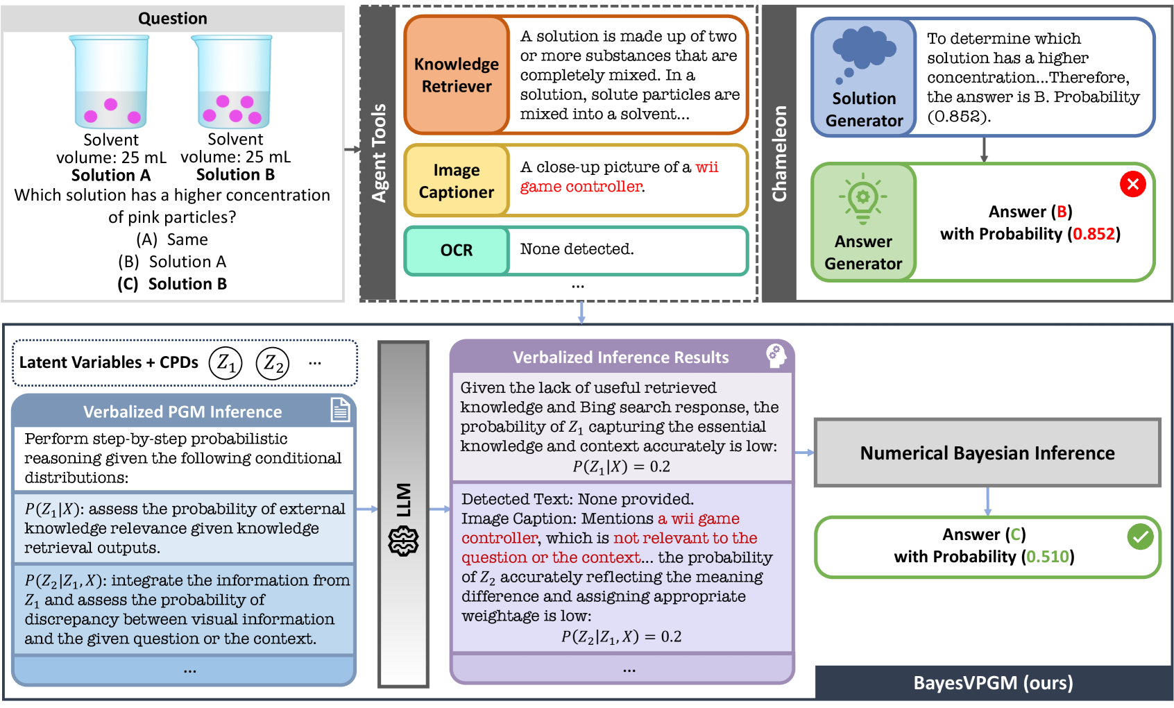
Figure 1: Example of inference using the BayesVPGM. The Chameleon framework erroneously assigns high confidence to the answer despite its LLM agents capturing irrelevant information. Conversely, our BayesVPGM accurately identifies this discrepancy and assigns low confidence. Here, we show a simplified inference prompt. See Appendix for detailed examples.
## Related Work
Research on large language models (LLMs) has recently transitioned from static prompting toward LLM agents or agentic systems capable of agentic reasoning, tool use, and interactive decision-making. We discuss both threads respectively, highlighting their limitations and how our proposed vPGM addresses a key missing component: probabilistic latent-variable reasoning and uncertainty calibration for agentic reasoning tasks.
#### LLM Prompting
Prompting methods in LLMs form a long-standing research line centered on training-free model responses steering. Early approaches include in-context learning (Brown et al. 2020), where models are conditioned on task-specific demonstrations, and instruction prompting (Wang et al. 2022b; Ouyang et al. 2022), which embeds explicit task instructions directly into natural-language prompts. A major development is Chain-of-Thought (CoT) prompting (Wei et al. 2022), which elicits intermediate reasoning steps to enhance complex reasoning. Subsequent variants extend CoT to more flexible or automated settings: zero-shot CoT (Kojima et al. 2022), automatic rationale generation (Auto-CoT) (Zhang et al. 2022; Shum, Diao, and Zhang 2023; Yao et al. 2024), self-consistency decoding (Wang et al. 2022a), and chain-of-continuous-thought (Hao et al. 2024), which embeds reasoning trajectories in a latent space. Additionally, (Xiong et al. 2023) built upon the consistency-based method and conducted an empirical study on confidence elicitation for LLMs. In contrast, our proposed vPGM tackles the confidence elicitation problem from the perspective of Bayesian inference, which follows the principles of a more theoretically grounded Bayesian inference framework, PGM.
#### LLM Agents and Agentic Systems
Building on these prompting advances, LLM prompting has evolved into LLM agents, which interleave reasoning with actions, tool use, and interaction with external environments. ReAct (Yao et al. 2023) combines natural-language reasoning with tool calls and environment feedback; Toolformer (Schick et al. 2023) uses self-supervised signals to teach LLMs when and how to invoke tools, and ADAS (Wang et al. 2025) automates the design of agentic system architectures. These systems mark a shift from passive text generation to interactive, tool-augmented behavior. However, existing agentic approaches typically lack a principled probabilistic framework: they do not explicitly model latent variables, quantify uncertainty, or perform Bayesian belief updating, which limits their applicability in settings that require calibrated agentic reasoning under uncertainty.
#### Concurrent Work
Several concurrent works explore the use of LLMs for probabilistic or causal modeling, but they are largely orthogonal to our contribution. Recent causal-discovery studies (Wan et al. 2025; Constantinou, Kitson, and Zanga 2025) focus on learning causal relationships and counterfactuals, whereas vPGM targets non-causal probabilistic latent-variable reasoning and uncertainty calibration for multi-source agentic tasks. BIRD (Feng et al. 2025) introduces a Bayesian inference wrapper for LLMs, yet it is restricted to binary decision-making and is therefore not directly applicable to our multi-class and open-ended outputs. In contrast, vPGM provides a unified Bayesian framework for latent-variable reasoning and calibrated uncertainty within LLM agents. footnotetext: Although we set $n\leq 4$ in this example, the LLM may generate the maximum number of variables. To reduce redundancies, we can add additional constraints to encourage a more compact representation.
## Our Method: Verbalized Probabilistic Graphical Modeling (vPGM)
Verbalized Probabilistic Graphical Modeling (vPGM) is a Bayesian Agentic Reasoning approach that leverages Large Language Models (LLM) agents to simulate key principles of Probabilistic Graphical Models (PGMs) in natural language. Unlike many existing probabilistic methods that demand extensive domain knowledge and specialized training, vPGM bypasses the need for expert-based model design, making it suitable for handling complex reasoning tasks where domain assumptions are limited or data are scarce.
### Overview of vPGM
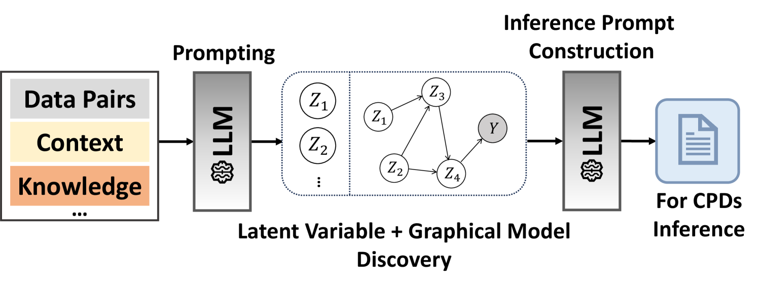
From an application standpoint, vPGM can be embedded into a range of complex reasoning systems, such as agentic reasoning tasks (see Figure 1). Our approach factorizes the overall reasoning process into three core steps: (1) Graphical Structure Discovery, in which the LLM is prompted to identify latent variables and their probabilistic dependencies (see Figure 2); (2) Prompting-Based Inference, where LLMs are guided to infer verbalized posterior distributions of each latent variable given new input data; and (3) Predictions under Uncertainty, where confidence in the final predictions is achieved by computing the expected value of the conditional predictive distribution over the inferred latent variables.
<details>
<summary>x2.png Details</summary>
### Visual Description
\n
## Diagram: Latent Variable and Graphical Model Discovery Pipeline
### Overview
The image depicts a pipeline for latent variable and graphical model discovery, utilizing Large Language Models (LLMs) at two stages: prompting and inference prompt construction. The pipeline takes data pairs, context, and knowledge as input, processes them through an LLM to discover a latent variable graphical model, and then uses another LLM to construct an inference prompt for Conditional Probability Distributions (CPDs) inference.
### Components/Axes
The diagram consists of three main sections, arranged horizontally from left to right:
1. **Input:** A rectangular block labeled "Data Pairs, Context, Knowledge..."
2. **Latent Variable + Graphical Model Discovery:** A rectangular block containing a graphical model with nodes labeled Z1, Z2, Z3, Z4, and Y, connected by directed edges. This block is labeled "Latent Variable + Graphical Model Discovery".
3. **Inference Prompt Construction:** A rectangular block labeled "Inference Prompt Construction" leading to an output labeled "For CPDs Inference".
Two LLM blocks are present, one between the input and the graphical model discovery block, and another between the graphical model discovery block and the inference prompt construction block.
### Detailed Analysis or Content Details
The input block contains the following labels:
* "Data Pairs"
* "Context"
* "Knowledge"
* "..." (indicating more inputs)
The graphical model within the "Latent Variable + Graphical Model Discovery" block consists of five nodes:
* Z1
* Z2
* Z3
* Z4
* Y
The connections (directed edges) are as follows:
* Z1 -> Z2
* Z1 -> Z3
* Z2 -> Y
* Z4 -> Y
* Z3 -> Z4
The output block is labeled "For CPDs Inference" and depicts a document icon.
### Key Observations
The diagram illustrates a two-stage process. The first stage uses an LLM to transform input data into a graphical model representing latent variables and their relationships. The second stage uses another LLM to generate an inference prompt, presumably for calculating CPDs based on the discovered graphical model. The diagram does not provide any numerical data or specific values. It is a conceptual illustration of a process.
### Interpretation
This diagram represents a novel approach to probabilistic modeling. Traditionally, graphical models are constructed by domain experts or through complex statistical algorithms. This pipeline proposes leveraging the reasoning capabilities of LLMs to automate the discovery of latent variable structures from raw data, context, and knowledge. The use of an LLM for inference prompt construction suggests a further integration of LLMs into the inference process, potentially enabling more flexible and interpretable probabilistic reasoning. The diagram highlights the potential of LLMs to bridge the gap between unstructured data and structured probabilistic models. The "..." in the input block suggests that the pipeline can accommodate various types of input data beyond just data pairs, context, and knowledge. The final output, "For CPDs Inference," indicates that the ultimate goal is to perform probabilistic inference using the discovered model.
</details>
Figure 2: Overview of the vPGM’s learning framework. CPDs represent conditional probability distributions. We omit the observed variable $\mathbf{X}$ for clarity.
### Graphical Structure Discovery
Our method begins by formulating a specialized prompt (see the appendix for the prompt) to uncover latent variables for compositional reasoning. The prompt comprises several key elements: (1) General Task Description, a concise statement of the reasoning objective; (2) Input-Output Data Pairs, which illustrate representative data samples; (3) Contextual Information, providing any essential background or domain insights; and (4) Prior Knowledge and Constraints, specifying constraints such as the maximum number of latent variables and predefined dependencies among them.
After identifying a set of latent variables $\mathbf{Z}=\{Z_{1},Z_{2},\ldots,Z_{n}\}$ (see the appendix for examples of latent variables) , we further prompt LLMs to determine how each latent variable depends on the others. An example set of dependencies obtained from the LLM is: $\{\mathbf{X}\rightarrow Z_{1},\mathbf{X}\rightarrow Z_{2},\mathbf{X}\rightarrow Z_{3},\mathbf{X}\rightarrow Z_{4},Z_{1}\rightarrow Z_{3},Z_{2}\rightarrow Z_{3},Z_{2}\rightarrow Z_{4},Z_{3}\rightarrow Z_{4},Z_{4}\rightarrow\mathbf{Y}\}$ , where each relationship $a\rightarrow b$ indicates that $b$ is conditionally dependent on $a$ . Like traditional PGMs, our verbalized PGM (vPGM) encodes these dependencies as conditional probability distributions $P\bigl(Z_{i}\mid\mathrm{Pa}(Z_{i})\bigr)$ . However, instead of relying on explicit distributional forms, vPGM uses natural language descriptions (see Appendix for detailed examples) to specify each conditional relationship, reducing the need for extensive domain expertise or parameter estimation.
### Prompting-Based Bayesian Inference
Traditionally, Bayesian inference focuses on inferring posterior distributions over model parameters given a probabilistic model and new observations. In the context of LLMs, however, it is reformulated as generating prompts that simulate posterior inference under the vPGM framework, leveraging its discovered structure and new observations. This approach leverages the advanced reasoning capabilities of LLMs to produce instructions enabling them to simulate Bayesian inference principles. An example prompt is: “Generate the prompt that guides LLMs through step-by-step probabilistic reasoning based on the provided task description, discovered PGM, and testing data…”
### Prediction Under Uncertainty
Agentic reasoning tasks often involve significant uncertainty. For instance, an LLM agent (e.g., an image captioner) may produce noisy outputs, introducing aleatoric uncertainty. Under the vPGM framework, this variability is captured by the verbalized posterior distributions of latent variables. After constructing the verbalized posterior $P(\mathbf{Z}\mid\mathbf{X})$ via prompting-based Bayesian inference, we quantify confidence in the final predictions by taking the expected value of $P(\mathbf{Y}\mid\mathbf{Z})$ over $\mathbf{Z}$ :
$$
\mathbb{E}_{P(\mathbf{Z}\mid\mathbf{X})}\bigl[P(\mathbf{Y}\mid\mathbf{Z})\bigr]\;\approx\;\sum_{\mathbf{Z}}P(\mathbf{Y}\mid\mathbf{Z})\,P(\mathbf{Z}\mid\mathbf{X}), \tag{1}
$$
where $\mathbf{X}$ denotes observed inputs, and $\mathbf{Z}$ is sampled by querying LLM using vPGM’s Bayesian inference prompt. In practice, both $P(\mathbf{Z}\mid\mathbf{X})$ and $P(\mathbf{Y}\mid\mathbf{Z})$ are simulated within a single prompt (see detailed examples in the Appendix). Consequently, the expected posterior probabilities can be approximated by averaging the numerical values of $P(\mathbf{Y}\mid\mathbf{Z})$ generated by the LLM during these inference steps.
## Bayesian-Enhanced vPGM: BayesVPGM
When repeatedly querying a Large Language Model (LLM) under the vPGM framework, we obtain multiple samples of responses, i.e., categorical predictions and their numerical probabilities. A natural question is how to leverage these data to better capture the underlying uncertainty in the LLM’s predictions. To do this, we propose to infer such a posterior distribution, denoted $q(\mathbf{y}\mid\tilde{\mathbf{x}})$ , where $\tilde{\mathbf{x}}$ denotes categorical predictions.
### Posterior Inference Under a Dirichlet Prior
We specify the form of the posterior $q(\mathbf{y}\mid\tilde{\mathbf{x}})\;=\;\mathrm{Cat}(\boldsymbol{\pi}),$ where $\boldsymbol{\pi}=(\pi_{1},\dots,\pi_{K})$ lies in the probability simplex over $K$ categories. To incorporate prior beliefs, we place a Dirichlet prior on $\boldsymbol{\pi}$ : $\boldsymbol{\pi}\;\sim\;\mathrm{Dirichlet}(\alpha_{1},\dots,\alpha_{K}),$ with $\alpha_{k}=\lambda\,p(y=k\mid\mathbf{Z})$ for some hyperparameter $\lambda>0$ , reflecting the vPGM’s initial belief in category $k$ .
Next, suppose we query the LLM under the vPGM framework for $n$ times, obtaining labels $\{y_{1},\dots,y_{n}\}$ . For each category $k$ , let $n_{k}$ be the number of labels that fall into that category. Assuming these labels are drawn i.i.d. from $\mathrm{Cat}(\boldsymbol{\pi})$ , the likelihood is $P\bigl(\{y_{i}\}\mid\boldsymbol{\pi}\bigr)\;=\;\prod_{k=1}^{K}\pi_{k}^{\,n_{k}}.$ By Bayes’ rule, the posterior distribution is then
$$
q(\mathbf{y}\mid\tilde{\mathbf{x}})\;\propto\;\Bigl(\prod_{k=1}^{K}\pi_{k}^{\,n_{k}}\Bigr)\times\Bigl(\prod_{k=1}^{K}\pi_{k}^{\,\alpha_{k}-1}\Bigr)\;=\;\prod_{k=1}^{K}\pi_{k}^{\,n_{k}+\alpha_{k}-1},
$$
i.e. a $\mathrm{Dirichlet}(n_{1}+\alpha_{1},\dots,n_{K}+\alpha_{K})$ . The posterior mean of $\pi_{k}$ becomes
$$
\pi_{k}^{(\mathrm{mean})}\;=\;\frac{n_{k}+\alpha_{k}}{\sum_{j=1}^{K}\bigl(n_{j}+\alpha_{j}\bigr)}.
$$
Consequently, we adopt $q(\mathbf{y}\mid\tilde{\mathbf{x}})\;=\;\mathrm{Cat}\bigl(\boldsymbol{\pi}^{(\mathrm{mean})}\bigr)$ as our final predictive distribution, which balances empirical label frequencies with the original vPGM’s numerical probabilities.
### Optimizing $\lambda$ via a Differentiable Calibration Loss
One key limitation of this posterior distribution is its reliance on a manually tuned $\lambda$ , which governs how strongly the vPGM’s numerical probabilities influence the final outcome. To automate this process and improve calibration, we introduce a differentiable calibration loss that learns $\lambda$ through gradient‐based optimization.
Specifically, we minimize the following loss function with respect to $\lambda$ :
$$
\mathcal{L}\bigl(\boldsymbol{\pi}(\lambda)\bigr)\;=\;\mathcal{L}_{c}\bigl(\boldsymbol{\pi}(\lambda)\bigr)\;+\;\beta\,\mathcal{L}_{v}\bigl(\boldsymbol{\pi}(\lambda)\bigr), \tag{2}
$$
where $\boldsymbol{\pi}(\lambda)=(\pi_{1}^{(\mathrm{mean})},\dots,\pi_{K}^{(\mathrm{mean})})$ is the posterior‐mean vector, $\mathcal{L}_{c}$ is a standard classification loss (e.g., cross‐entropy), and $\mathcal{L}_{v}$ is a differentiable class‐wise alignment term; $\beta$ is a hyperparameter balancing the two losses. Let $j$ index the categories, and let $\bar{\pi}_{j}=\frac{1}{n}\sum_{i=1}^{n}\pi_{j}^{(i)}$ be the average predicted probability of class $j$ over a mini‐batch of size $n$ . Likewise, let $\bar{y}_{j}=\frac{1}{n}\sum_{i=1}^{n}y_{j}^{(i)}$ be the empirical fraction of class $j$ , where $y_{j}^{(i)}\in\{0,1\}$ indicates whether sample $i$ belongs to class $j$ . Inspired by class‐wise expected calibration error (Kull et al. 2019), which aligns predictions to empirical frequencies on a per‐category basis but whose binning procedure impedes differentiability, we define:
$$
\mathcal{L}_{v}\bigl(\boldsymbol{\pi}\bigr)\;=\;\frac{1}{K}\sum_{j=1}^{K}\Bigl|\bar{\pi}_{j}\;-\;\bar{y}_{j}\Bigr|, \tag{3}
$$
using a bin‐free version of class-wise expected calibration error.
To minimize $\mathcal{L}\bigl(\boldsymbol{\pi}\bigr)$ with respect to $\lambda$ , we employ a quasi‐Newton method (e.g., L-BFGS) (Broyden 1967). This second‐order gradient‐based solver converges more rapidly than simple gradient descent.
**Theorem 1 (Global Optimum Implies Perfect ECE)**
*Let $\{(\mathbf{u}_{i},y_{i})\}_{i=1}^{n}$ be the training set with features $\mathbf{u}_{i}\in\mathbb{R}^{d}$ and one–hot labels $y_{ik}$ . For any parameter vector $\theta$ , let $g_{\theta}:\mathbb{R}^{d}\!\to\!\Delta^{K-1}$ be a function that produces class probabilities $\widehat{p}_{ik}(\theta)=g_{\theta}(\mathbf{u}_{i})_{k}$ . The empirical version of Eq. (2) is
$$
\mathcal{L}(\theta)=-\frac{1}{n}\sum_{i=1}^{n}\sum_{k=1}^{K}y_{ik}\,\log\widehat{p}_{ik}(\theta)+\beta\,\frac{1}{K}\sum_{k=1}^{K}\bigl|\bar{\widehat{p}}_{k}(\theta)-\bar{y}_{k}\bigr|,
$$
where $\beta>0,\bar{\widehat{p}}_{k}(\theta)=\tfrac{1}{n}\sum_{i}\widehat{p}_{ik}(\theta)$ , and $\bar{y}_{k}=\tfrac{1}{n}\sum_{i}y_{ik}$ . Then a parameter vector $\theta^{\star}$ is a global minimiser of $\mathcal{L}$ iff
| | | $\displaystyle\widehat{p}_{ik}(\theta^{\star})=\frac{1}{\sum_{i^{\prime}=1}^{n}\mathbb{I}_{\{\mathbf{u}_{i}=\mathbf{u}_{i^{\prime}}\}}}\sum_{i^{\prime}=1}^{n}y_{i^{\prime}k}\mathbb{I}_{\{\mathbf{u}_{i}=\mathbf{u}_{i^{\prime}}\}}$ | |
| --- | --- | --- | --- |
where $\mathbb{I}(\mathbf{u}_{i}=\mathbf{u}_{i^{\prime}})$ is an indicator function equal to 1 if the feature inputs $\mathbf{u}_{i}$ and $\mathbf{u}_{i^{\prime}}$ are identical, and 0 otherwise. In that case, the class-wise expected calibration error $\operatorname{ECE}_{\mathrm{class}}(\theta)\triangleq\frac{1}{K}\sum_{k}|\bar{\widehat{p}}_{k}(\theta)-\bar{y}_{k}|$ satisfies $\operatorname{ECE}_{\mathrm{class}}(\theta^{\star})=0$ .*
The proof is provided in Appendix. Although the cross-entropy term in the loss function Eq. (2) pulls predictions toward one-hot labels while the calibration term enforces class-wise average alignment, Theorem 1 shows that both objectives can attain their minima simultaneously.
## Experiments
We evaluate the efficacy of the proposed vPGM and BayesVPGM in modeling uncertainty across three agentic reasoning tasks. The first, a closed-ended task named ScienceQA (Lu et al. 2022), and the second, an open-ended task named ChatCoach (Huang et al. 2024), both require reasoning with undisclosed information from multiple sources. We then introduce a negative control experiment derived from A-OKVQA (Schwenk et al. 2022) to investigate whether latent variables can enhance confidence calibration by detecting mismatches in the presence of misinformation. See Appendix for the detailed experimental configurations.
### Science Question Answering
The Science Question Answering (ScienceQA) benchmark, introduced by (Lu et al. 2022), serves as a comprehensive benchmark for multi-modal question answering across a diverse range of scientific disciplines, including physics, mathematics, biology, and the humanities. It features 4,241 question-answer pairs that cover various topics and contexts. This task demands the integration of information from multiple sources or LLM agents (e.g., Bing search results, image captions), a process that can introduce errors and increase the complexity of reasoning. Given these challenges, ScienceQA serves as an ideal testbed for evaluating how effectively vPGM identifies latent structures and model uncertainties. See Appendix for the more detailed experimental setups.
#### Baseline Methods
We compare vPGM/BayesVPGM with the following baseline methods:
- Chain-of-Thought This is one of the non-tool-augmented LLMs: Chain-of-Thought (CoT) prompting (Wei et al. 2022) equipped with verbalized confidence estimation by prompting it to provide a numerical confidence for the selected answer.
- Chameleon This is based on a tool-augmented LLM: Chameleon (Lu et al. 2023), and we equip it with verbalized confidence estimation.
- Chameleon+ It extends Chameleon with a state-of-art uncertainty quantification framework based on the combination of verbalized confidence estimation and self-consistency measurement (Wang et al. 2022a), as recommended in (Xiong et al. 2023).
#### Evaluation Metrics
In line with previous evaluation settings in (Naeini, Cooper, and Hauskrecht 2015; Guo et al. 2017; Xiong et al. 2023) on confidence calibration, we adopt the expected calibration error (ECE) to evaluate model confidence, represented as numeric probabilistic predictions. The ECE quantifies the divergence between the predicted probabilities and the observed accuracy across each confidence levels (bins). Throughout our experiments, we fix the number of confidence bins as 10 with uniform confidence contribution across bins. In addition, we evaluate the capability of a given method in solving problems correctly by measuring the accuracy (Acc.).
| CoT | – | 1 | 84.63 | 8.96 |
| --- | --- | --- | --- | --- |
| Chameleon | – | 1 | 85.29 | 9.62 |
| Chameleon+ | – | 3 | 85.17 | 8.65 |
| vPGM (Ours) | 2 | 3 | 85.49 | 2.31 |
| vPGM (Ours) | 3 | 3 | 86.38 | 1.67 |
| vPGM (Ours) | 4 | 3 | 86.54 | 2.15 |
| BayesVPGM (Ours) | 2 | 3 | 85.49 | 1.81 |
| BayesVPGM (Ours) | 3 | 3 | 86.38 | 1.05 |
| BayesVPGM (Ours) | 4 | 3 | 86.54 | 1.50 |
Table 1: Accuracy ( $\$ ) and ECE $(\times 10^{2})$ on ScienceQA for different methods and numbers of latent variables $N$ . $M$ is the number of sampled responses. The best and second-best results within each base model are bolded and underlined, respectively. Llama3-8B-Instruct (Dubey et al. 2024) serves as our test-time engine. See appendix for results using other LLMs
#### Results
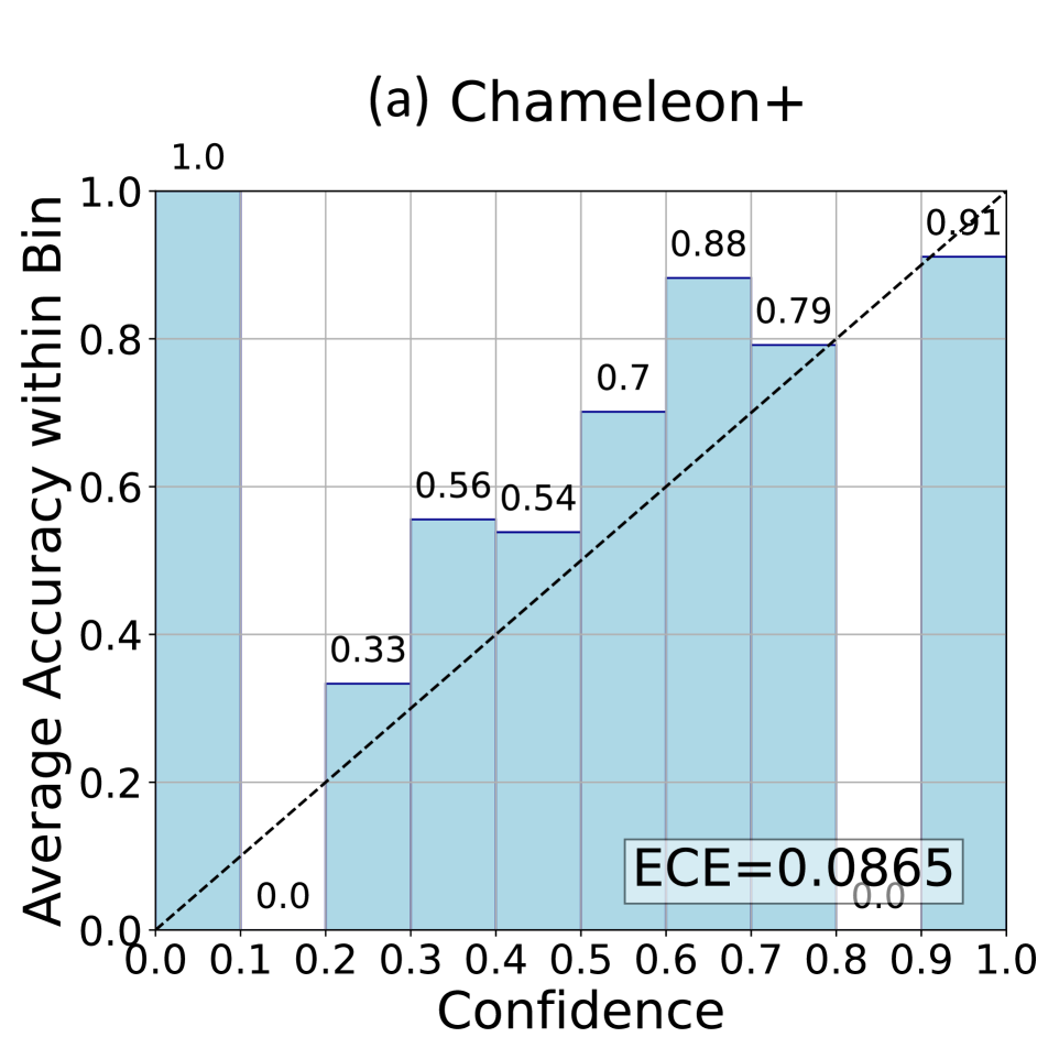
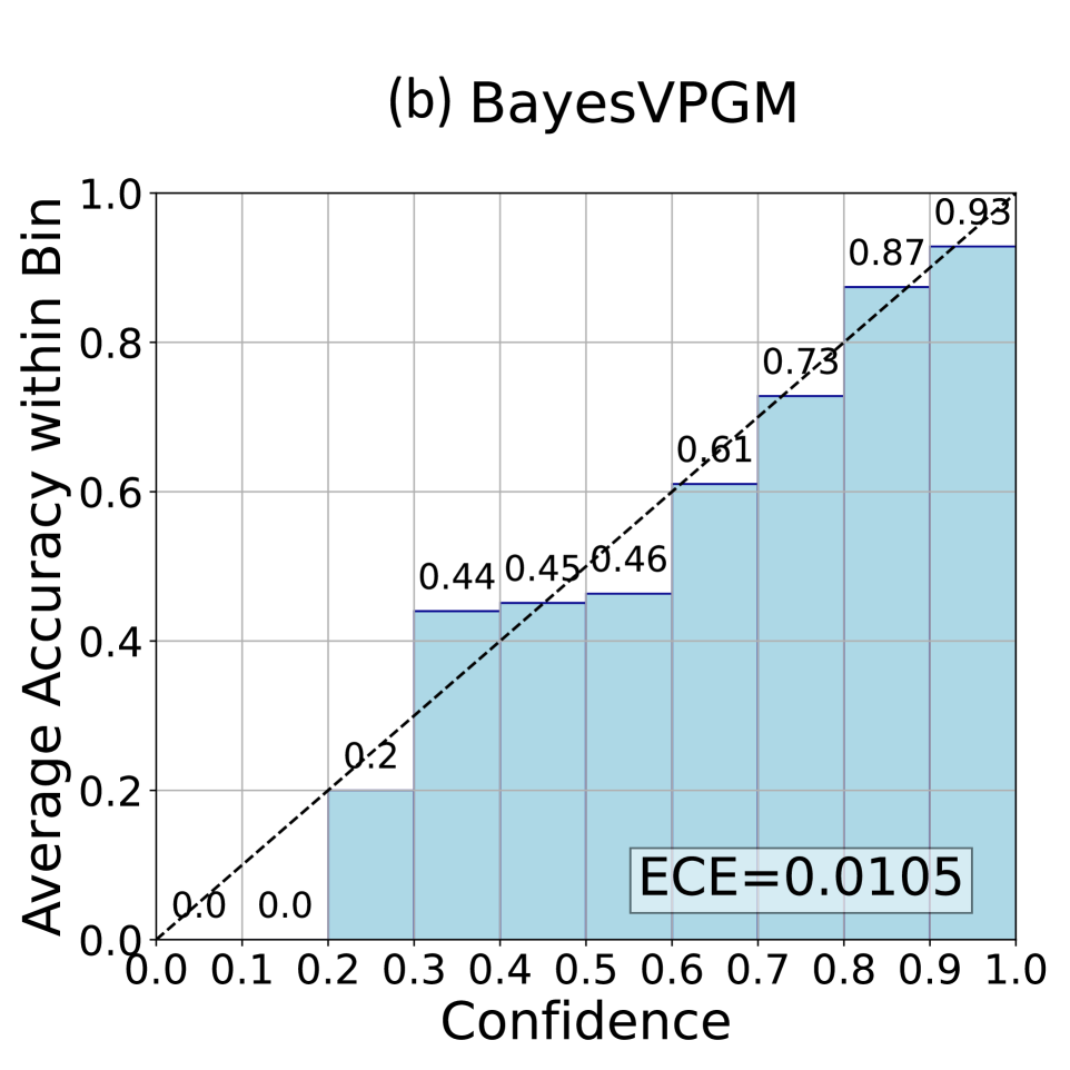
Table 1 details the performance of different methods on the ScienceQA dataset. It shows that Chameleon results in the highest (worst) ECE ( $\times 10^{2}$ ) of 9.62, indicating serious overconfidence issues in handling complex reasoning tasks, even with the assistance of external tools. In comparison, our vPGM outperforms these methods in both accuracy and ECE, due to its superior ability to capture latent structural information that other baseline methods overlook. Figure 3 shows the reliability diagram for vPGM and BayesVPGM, demonstrating its near-perfect alignment with the ideal calibration curve across all bins, highlighting its precision in confidence calibration (see the Appendix for the ablation results and the token-level computational costs).
#### Qualitative Study on the Inferred Latent Variables
Figure 1 shows a case study of BayesVPGM’s inference capabilities to qualitatively assess the model’s ability to utilize latent structural information for improving confidence estimation. Here vPGM employs its latent variables to critically assess the relevance of retrieved information. For example, when faced with irrelevant data from external tools such as Bing search or inaccurate captions from image captioners, the baseline, Chameleon, erroneously maintains high confidence in its predictions. In contrast, BayesVPGM carefully adjusts its confidence, assigning lower probabilities when essential contextual knowledge is missing or incorrect, a process that is particularly effective through the inference of latent variables $Z_{1}$ and $Z_{2}$ . These observations highlight the significance of inferring latent structures to improve the reliability of compositional reasoning systems.
<details>
<summary>x3.png Details</summary>
### Visual Description
## Reliability Diagram: Chameleon+
### Overview
This image presents a reliability diagram, also known as a calibration plot, for a model named "Chameleon+". The diagram assesses the model's confidence in its predictions against the actual accuracy of those predictions. It visualizes how well the predicted probabilities align with the observed frequencies.
### Components/Axes
* **Title:** (a) Chameleon+ - positioned at the top-center of the image.
* **X-axis:** Confidence - ranging from 0.0 to 1.0, with markers at 0.1, 0.2, 0.3, 0.4, 0.5, 0.6, 0.7, 0.8, 0.9, and 1.0.
* **Y-axis:** Average Accuracy within Bin - ranging from 0.0 to 1.0, with markers at 0.1, 0.2, 0.3, 0.4, 0.5, 0.6, 0.7, 0.8, 0.9, and 1.0.
* **Data Points:** Rectangular blocks representing the average accuracy for predictions falling within specific confidence bins. Each block contains a numerical value representing the average accuracy.
* **Calibration Line:** A dashed black line representing perfect calibration (i.e., predicted probability equals observed frequency).
* **ECE Value:** A text label "ECE=0.0865" indicating the Expected Calibration Error, positioned in the bottom-right corner.
### Detailed Analysis
The diagram is divided into ten bins along the confidence axis, each representing a range of predicted probabilities. The height of each block corresponds to the average accuracy of predictions within that bin.
Here's a breakdown of the data points, moving from left to right (low confidence to high confidence):
* **Bin 1 (0.0 - 0.1):** Average Accuracy = 0.0
* **Bin 2 (0.1 - 0.2):** Average Accuracy = 0.33
* **Bin 3 (0.2 - 0.3):** Average Accuracy = 0.56
* **Bin 4 (0.3 - 0.4):** Average Accuracy = 0.54
* **Bin 5 (0.4 - 0.5):** Average Accuracy = 0.7
* **Bin 6 (0.5 - 0.6):** Average Accuracy = 0.79
* **Bin 7 (0.6 - 0.7):** Average Accuracy = 0.88
* **Bin 8 (0.7 - 0.8):** Average Accuracy = 0.91
* **Bin 9 (0.8 - 0.9):** Average Accuracy = 0.91
* **Bin 10 (0.9 - 1.0):** Average Accuracy = 0.91
The calibration line starts at (0.0, 0.0) and ends at (1.0, 1.0). The data points generally trend upwards, indicating that as confidence increases, accuracy also tends to increase. However, the data points do not perfectly align with the calibration line, indicating some degree of miscalibration.
### Key Observations
* The model is significantly underconfident in the low-confidence region (0.0 - 0.3), as the accuracy is considerably higher than the confidence.
* The model appears to be well-calibrated in the high-confidence region (0.7 - 1.0), with accuracy values close to the confidence levels.
* The ECE value of 0.0865 suggests a relatively low degree of miscalibration overall.
### Interpretation
The reliability diagram demonstrates that the "Chameleon+" model is generally well-calibrated, but exhibits some underconfidence in the lower confidence ranges. This means that when the model is less certain about its predictions, it tends to be more accurate than its stated confidence suggests. The low ECE value confirms this overall good calibration.
The diagram is useful for understanding the trustworthiness of the model's predictions. A well-calibrated model is desirable because it allows users to appropriately weigh the risks associated with relying on its outputs. In this case, users might consider giving more weight to predictions made with low confidence, as they may be more accurate than initially indicated. The calibration line serves as a benchmark for assessing the model's performance, and deviations from this line highlight areas where the model's confidence may be misaligned with its actual accuracy.
</details>
<details>
<summary>x4.png Details</summary>
### Visual Description
## Reliability Diagram: BayesVPGM
### Overview
This image presents a reliability diagram, also known as a calibration plot, for a model named BayesVPGM. The diagram visualizes the relationship between the model's confidence in its predictions and the actual accuracy of those predictions. It's a square heatmap-like chart with confidence on the x-axis and average accuracy within bins on the y-axis. A diagonal line represents perfect calibration.
### Components/Axes
* **Title:** (b) BayesVPGM – Located at the top-center of the image.
* **X-axis:** Confidence – Ranges from 0.0 to 1.0, with markers at 0.1 intervals.
* **Y-axis:** Average Accuracy within Bin – Ranges from 0.0 to 1.0, with markers at 0.1 intervals.
* **Color Scale:** The chart uses a light blue color gradient to represent the density or frequency of predictions falling into each confidence/accuracy bin. Darker shades indicate higher frequency.
* **Calibration Line:** A dashed black line represents the ideal calibration, where confidence equals accuracy.
* **ECE Value:** A white box in the bottom-right corner displays the Expected Calibration Error (ECE) value.
### Detailed Analysis
The chart is divided into a grid of bins, each representing a range of confidence levels and corresponding accuracy levels. The values within each bin represent the average accuracy for predictions made with a confidence level falling within that bin.
Here's a breakdown of the values observed in each bin, reading from bottom-left to top-right:
* **(0.0 - 0.1, 0.0 - 0.1):** 0.0
* **(0.1 - 0.2, 0.0 - 0.1):** 0.0
* **(0.2 - 0.3, 0.1 - 0.2):** 0.2
* **(0.3 - 0.4, 0.3 - 0.4):** 0.44
* **(0.4 - 0.5, 0.4 - 0.5):** 0.45
* **(0.4 - 0.5, 0.5 - 0.6):** 0.46
* **(0.5 - 0.6, 0.5 - 0.6):** 0.61
* **(0.6 - 0.7, 0.6 - 0.7):** 0.73
* **(0.7 - 0.8, 0.7 - 0.8):** 0.87
* **(0.8 - 0.9, 0.8 - 0.9):** 0.93
* **(0.9 - 1.0, 0.9 - 1.0):** 0.93
The dashed calibration line starts at approximately (0.0, 0.0) and ends at approximately (1.0, 1.0). The values within the bins generally follow an upward trend, indicating that as confidence increases, accuracy also tends to increase. However, the values are not perfectly aligned with the calibration line, indicating some degree of miscalibration.
The ECE value, displayed in the bottom-right corner, is 0.0105.
### Key Observations
* The model is generally well-calibrated, as the values are relatively close to the diagonal calibration line.
* The model appears to be slightly underconfident in the lower confidence ranges (0.0-0.4) and slightly overconfident in the higher confidence ranges (0.8-1.0).
* The ECE value of 0.0105 suggests a low level of miscalibration.
### Interpretation
This reliability diagram demonstrates that the BayesVPGM model is reasonably well-calibrated. The model's confidence levels generally align with its actual accuracy, although there are some minor deviations. The low ECE value confirms this observation.
The diagram suggests that the model's predictions are reliable, meaning that when the model expresses high confidence in a prediction, it is likely to be accurate, and vice versa. This is important for applications where it is crucial to have a good understanding of the uncertainty associated with the model's predictions.
The slight underconfidence in lower confidence ranges could indicate that the model is hesitant to make strong predictions when it is uncertain, which is a conservative approach. The slight overconfidence in higher confidence ranges could be a result of the model being overly optimistic about its predictions when it is very certain.
</details>
Figure 3: Reliability diagrams of (a) Chameleon+ and (b) BayesVPGM ( $N=3,M=3$ ) on ScienceQA (see the appendix for diagrams of Chameleon and vPGM). BayesVPGM achieve a much lower ECE comparing to Chameleon+ and approaches to the ideal confidence calibration curve (the diagonal dashed line).
| Instruction Prompting Vanilla CoT Zero-shot CoT | 27.4 17.7 27.6 | 3.3 2.7 1.9 | 67.6 64.1 69.0 | 1.4 0.1 3.0 | 2.1 2.3 0.9 | 61.6 58.1 58.8 |
| --- | --- | --- | --- | --- | --- | --- |
| GCoT | 34.2 | 3.7 | 72.4 | 1.6 | 2.0 | 65.4 |
| vPGM (Ours) | 37.2 | 2.3 | 76.3 | 1.7 | 2.0 | 68.3 |
| Human | 76.6 | 6.0 | 90.5 | 33.5 | 3.6 | 84.1 |
Table 2: Results of various methods on the detection and correction of medical terminology errors.
### Communicative Medical Coaching
The Communicative Medical Coaching benchmark, ChatCoach, introduced in (Huang et al. 2024), establishes a complex multi-agent dialogue scenario involving doctors, patients, and a medical coach across 3,500 conversation turns. The medical coach is tasked with detecting inaccuracies in medical terminology used by doctors (detection task) and suggesting appropriate corrections (correction task). These tasks require integrating external medical knowledge, inherently introducing uncertainty into response formulation. This benchmark was chosen to test vPGM’s ability to generalize across complex open-ended reasoning tasks. BayesVPGM is not applied in this setting, as such a model assumes the output to be a categorical distribution. See the Appendix for more details on experiments and implementation.
#### Baseline Methods
For comparative analysis, we benchmark vPGM against these approaches:
- Vanilla Instruction Prompting: This method involves prompting the LLM with direct instructions for dialogue generation.
- Zero-shot Chain of Thought (CoT) (Kojima et al. 2022): A straightforward CoT approach where the LLM is prompted to sequentially articulate a reasoning chain.
- Vanilla CoT (Wei et al. 2022): This method builds upon the basic CoT by providing the LLM with a set of examples that include detailed reasoning steps.
- Generalized CoT (GCoT) (Huang et al. 2024): An advanced version of CoT, designed to improve the generation of structured feedback and integration of external knowledge effectively. It represents a state-of-the-art method in the ChatCoach benchmark.
#### Evaluation Metrics
We follow (Huang et al. 2024) to employ conventional automated metrics BLEU-2, ROUGE-L, and BERTScore. BLEU-2 is employed to measure the precision of bi-gram overlaps, offering insights into the lexical accuracy of the generated text against reference answers. ROUGE-L is used to assess sentence-level similarity, focusing on the longest common subsequence to evaluate structural coherence and the alignment of sequential n-grams. Additionally, BERTScore is applied for a semantic similarity assessment, utilizing BERT embeddings to compare the generated outputs and reference texts on a deeper semantic level. As specified in (Huang et al. 2024), we use GPT-4 to extract medical terminology errors and corresponding corrections in the feedback from Coach Agents. Automated metrics are then calculated based on these extracted elements in comparison to human annotations.
#### Results
We present the performance of various methods in Table 2. The noticeable difference between machine-generated outputs and human benchmarks across all metrics highlights the inherent challenges in communicative medical coaching. In the detection of medical terminology errors, vPGM leads with superior BLEU-2 (37.2) and BERTScore (76.3), underscoring its proficiency in identifying inaccuracies. In the correction task, while vPGM achieves a standout BERTScore of 68.3, surpassing all baselines, it scores lower on BLEU-2 and ROUGE-L. This variation is attributed to the ambiguity in doctors’ inputs, which can yield multiple valid responses, affecting metrics that rely on exact matches.
### A-OKVQA Negative Control: Studying Latent Variables Under Misinformation
#### Data Simulation
A-OKVQA (Schwenk et al. 2022) is a Visual Question Answering dataset that challenges models to perform commonsense reasoning about a scene, often beyond the reach of simple knowledge-base queries. Crucially, it provides ground-truth image captions and rationales for each question. We leverage these annotations to construct a negative control experiment: A-OKVQA-clean (603 data points) retains the correct image caption and rationale (near single-hop reasoning), while A-OKVQA-noisy (603 data points) randomly shuffles the rationale, thus introducing misinformation and forcing a multi-hop check for consistency. In this experiment, we adopt a vPGM with 2 latent variables (see the Appendix for the inference prompt and an example query). Refer to the Appendix for more details on data configurations.
#### Overall Performance Under Noisy Conditions
Table 3 shows the overall accuracy (Acc.) and expected calibration error (ECE) on the A-OKVQA-noisy dataset. Both vPGM and BayesVPGM outperform Chameleon+ on accuracy (61.03% vs. 59.04%) and yield lower ECE, indicating that latent variables detect mismatch and improve confidence calibration.
#### Mismatch Detection Through $Z_{2}$
To investigate how latent variables facilitate mismatch detection, we track $P\bigl(Z_{2}\mid\mathrm{Pa}(Z_{2})\bigr)$ , where $Z_{2}$ indicates whether the rationale is aligned with the image caption. As shown in Table 4, the mean probability of $Z_{2}$ is considerably higher in the Clean set than in the Noisy set (0.86 vs. 0.42), and mismatch identification accuracy in the Noisy condition reaches 87%. These findings demonstrate BayesVPGM’s capacity to robustly detect cases with inconsistencies or irrelevant content.
#### Latent Variable Correlation Analysis
We additionally compute Pearson correlations (Pcc.) between numerical conditional probabilities of the latent variables ( $Z_{1}$ and $Z_{2}$ ) and the final answer $\mathbf{Y}$ . In the Noisy case, $\text{Pcc}(Z_{2},\mathbf{Y})$ surpasses $\text{Pcc}(Z_{1},\mathbf{Y})$ (0.55 versus 0.35), indicating that $Z_{2}$ exerts a stronger influence on the final prediction when mismatches are present. Conversely, in the Clean subset, $Z_{1}$ and $Z_{2}$ exhibit nearly equal correlation with $\mathbf{Y}$ , yet about 22% of the Clean data is incorrectly flagged by $Z_{2}$ as mismatched, potentially introducing noisy confidence adjustments at $\mathbf{Y}$ . This suggests a trade-off: while latent variables excel at detecting misinformation and improving calibration in Noisy settings, they can slightly degrade calibration when no mismatch actually exists.
| Chameleon+ vPGM (Ours) BayesVPGM (Ours) | 59.04 61.03 61.03 | 11.75 10.54 9.85 |
| --- | --- | --- |
Table 3: General Performance on A-OKVQA-noisy data (accuracy in $\$ and ECE in $\times 10^{2}$ ).
| Mean $P\bigl(Z_{2}\mid\mathrm{Pa}(Z_{2})\bigr)$ Noise Identification Acc. $\text{Pcc}\bigl(Z_{1},\mathbf{Y}\bigr)$ | 0.86 78% 0.50 | 0.42 87% 0.35 |
| --- | --- | --- |
| $\text{Pcc}\bigl(Z_{2},\mathbf{Y}\bigr)$ | 0.51 | 0.55 |
Table 4: Analysis of the latent variables on A-OKVQA-clean and A-OKVQA-noisy.
## Conclusion
We introduce verbalized Probabilistic Graphical Model (vPGM), a Bayesian agentic framework that (1) directs LLM agents to simulate core principles of Probabilistic Graphical Models (PGMs) through natural language and (2) refines the resulting posterior distributions via numerical Bayesian inference. Applied within agentic workflows, vPGM enables LLM agents to perform probabilistic latent-variable reasoning with calibrated uncertainty. This approach discovers latent variables and dependencies without requiring extensive domain expertise, making it well-suited to settings with limited assumptions. Our empirical results on agentic reasoning tasks demonstrate substantial improvements in terms of both confidence calibration and text generation quality. These results highlight the potential of merging Bayesian principles with LLM agents to enhance AI systems’ capacity for modeling uncertainty and reasoning under uncertainty.
## Acknowledgments
We thank all reviewers, SPC, and AC for their valuable comments. S.B. acknowledges funding from the MRC Centre for Global Infectious Disease Analysis (reference MR/X020258/1), funded by the UK Medical Research Council (MRC). This UK funded award is carried out in the frame of the Global Health EDCTP3 Joint Undertaking. S.B. is funded by the National Institute for Health and Care Research (NIHR) Health Protection Research Unit in Modelling and Health Economics, a partnership between UK Health Security Agency, Imperial College London and LSHTM (grant code NIHR200908). H.W. is partially supported by Amazon Faculty Research Award, Microsoft AI & Society Fellowship, NSF CAREER Award IIS-2340125, NIH grant R01CA297832, and NSF grant IIS-2127918. We acknowledge support from OpenAI’s Researcher Access Program. Disclaimer: “The views expressed are those of the author(s) and not necessarily those of the NIHR, UK Health Security Agency or the Department of Health and Social Care.” S.B. acknowledges support from the Novo Nordisk Foundation via The Novo Nordisk Young Investigator Award (NNF20OC0059309). S.B. acknowledges the Danish National Research Foundation (DNRF160) through the chair grant. S.B. acknowledges support from The Eric and Wendy Schmidt Fund For Strategic Innovation via the Schmidt Polymath Award (G-22-63345) which also supports H.H. and L.M.
## References
- Abdullah, Hassan, and Mustafa (2022) Abdullah, A. A.; Hassan, M. M.; and Mustafa, Y. T. 2022. A review on bayesian deep learning in healthcare: Applications and challenges. IEEE Access, 10: 36538–36562.
- Achiam et al. (2023) Achiam, J.; Adler, S.; Agarwal, S.; Ahmad, L.; Akkaya, I.; Aleman, F. L.; Almeida, D.; Altenschmidt, J.; Altman, S.; Anadkat, S.; et al. 2023. Gpt-4 technical report. arXiv preprint arXiv:2303.08774.
- Bender and Koller (2020) Bender, E. M.; and Koller, A. 2020. Climbing towards NLU: On meaning, form, and understanding in the age of data. In Proceedings of the 58th Annual Meeting of the Association for Computational Linguistics, 5185–5198.
- Bielza and Larrañaga (2014) Bielza, C.; and Larrañaga, P. 2014. Bayesian networks in neuroscience: a survey. Frontiers in Computational Neuroscience, 8: 131.
- Brown et al. (2020) Brown, T.; Mann, B.; Ryder, N.; Subbiah, M.; Kaplan, J. D.; Dhariwal, P.; Neelakantan, A.; Shyam, P.; Sastry, G.; Askell, A.; et al. 2020. Language models are few-shot learners. Advances in neural information processing systems, 33: 1877–1901.
- Broyden (1967) Broyden, C. G. 1967. Quasi-Newton methods and their application to function minimisation. Mathematics of Computation, 21(99): 368–381.
- Constantinou, Kitson, and Zanga (2025) Constantinou, A. C.; Kitson, N. K.; and Zanga, A. 2025. Using GPT-4 to Guide Causal Machine Learning. Expert Systems with Applications.
- Devlin et al. (2018) Devlin, J.; Chang, M.-W.; Lee, K.; and Toutanova, K. 2018. Bert: Pre-training of deep bidirectional transformers for language understanding. arXiv preprint arXiv:1810.04805.
- Dubey et al. (2024) Dubey, A.; Jauhri, A.; Pandey, A.; Kadian, A.; Al-Dahle, A.; Letman, A.; Mathur, A.; Schelten, A.; Yang, A.; Fan, A.; et al. 2024. The llama 3 herd of models. arXiv e-prints, arXiv–2407.
- Feng et al. (2025) Feng, Y.; Zhou, B.; Lin, W.; and Roth, D. 2025. BIRD: A Trustworthy Bayesian Inference Framework for Large Language Models. In International Conference on Learning Representations (ICLR).
- Griffiths, Kemp, and Tenenbaum (2008) Griffiths, T. L.; Kemp, C.; and Tenenbaum, J. B. 2008. Bayesian models of cognition. In Annual Meeting of the Cognitive Science Society, 2004; This chapter is based in part on tutorials given by the authors at the aforementioned conference as well as the one held in 2006. Cambridge University Press.
- Guo et al. (2017) Guo, C.; Pleiss, G.; Sun, Y.; and Weinberger, K. Q. 2017. On calibration of modern neural networks. In International Conference on Machine Learning, 1321–1330. PMLR.
- Hao et al. (2024) Hao, S.; Sukhbaatar, S.; Su, D.; Li, X.; Hu, Z.; Weston, J.; and Tian, Y. 2024. Training large language models to reason in a continuous latent space. arXiv preprint arXiv:2412.06769.
- Huang et al. (2024) Huang, H.; Wang, S.; Liu, H.; Wang, H.; and Wang, Y. 2024. Benchmarking Large Language Models on Communicative Medical Coaching: a Novel System and Dataset. In Findings of the Association for Computational Linguistics: ACL 2024.
- Kitson et al. (2023) Kitson, N. K.; Constantinou, A. C.; Guo, Z.; Liu, Y.; and Chobtham, K. 2023. A survey of Bayesian Network structure learning. Artificial Intelligence Review, 56(8): 8721–8814.
- Kojima et al. (2022) Kojima, T.; Gu, S. S.; Reid, M.; Matsuo, Y.; and Iwasawa, Y. 2022. Large language models are zero-shot reasoners. Advances in Neural Information Processing Systems, 35: 22199–22213.
- Kull et al. (2019) Kull, M.; Perello Nieto, M.; Kängsepp, M.; Silva Filho, T.; Song, H.; and Flach, P. 2019. Beyond temperature scaling: Obtaining well-calibrated multi-class probabilities with dirichlet calibration. Advances in Neural Information Processing Systems, 32.
- Lake et al. (2017) Lake, B. M.; Ullman, T. D.; Tenenbaum, J. B.; and Gershman, S. J. 2017. Building machines that learn and think like people. Behavioral and Brain Sciences, 40: e253.
- Lu et al. (2022) Lu, P.; Mishra, S.; Xia, T.; Qiu, L.; Chang, K.-W.; Zhu, S.-C.; Tafjord, O.; Clark, P.; and Kalyan, A. 2022. Learn to explain: Multimodal reasoning via thought chains for science question answering. Advances in Neural Information Processing Systems, 35: 2507–2521.
- Lu et al. (2023) Lu, P.; Peng, B.; Cheng, H.; Galley, M.; Chang, K.-W.; Wu, Y. N.; Zhu, S.-C.; and Gao, J. 2023. Chameleon: Plug-and-play compositional reasoning with large language models. arXiv preprint arXiv:2304.09842.
- Naeini, Cooper, and Hauskrecht (2015) Naeini, M. P.; Cooper, G.; and Hauskrecht, M. 2015. Obtaining well calibrated probabilities using bayesian binning. In Proceedings of the AAAI Conference on Artificial Intelligence, volume 29.
- Ouyang et al. (2022) Ouyang, L.; Wu, J.; Jiang, X.; Almeida, D.; Wainwright, C.; Mishkin, P.; Zhang, C.; Agarwal, S.; Slama, K.; Ray, A.; et al. 2022. Training language models to follow instructions with human feedback. Advances in Neural Information Processing Systems, 35: 27730–27744.
- Schick et al. (2023) Schick, T.; Dwivedi-Yu, J.; Dessì, R.; Raileanu, R.; Lomeli, M.; Hambro, E.; Zettlemoyer, L.; Cancedda, N.; and Scialom, T. 2023. Toolformer: Language models can teach themselves to use tools. Advances in Neural Information Processing Systems, 36: 68539–68551.
- Schwenk et al. (2022) Schwenk, D.; Khandelwal, A.; Clark, C.; Marino, K.; and Mottaghi, R. 2022. A-okvqa: A benchmark for visual question answering using world knowledge. In European Conference on Computer Vision, 146–162. Springer.
- Shum, Diao, and Zhang (2023) Shum, K.; Diao, S.; and Zhang, T. 2023. Automatic Prompt Augmentation and Selection with Chain-of-Thought from Labeled Data. arXiv preprint arXiv:2302.12822.
- Sumers et al. (2023) Sumers, T. R.; Yao, S.; Narasimhan, K.; and Griffiths, T. L. 2023. Cognitive architectures for language agents. arXiv preprint arXiv:2309.02427.
- Tenenbaum et al. (2011) Tenenbaum, J. B.; Kemp, C.; Griffiths, T. L.; and Goodman, N. D. 2011. How to grow a mind: Statistics, structure, and abstraction. Science, 331(6022): 1279–1285.
- Wan et al. (2025) Wan, G.; Lu, Y.; Wu, Y.; Hu, M.; and Li, S. 2025. Large Language Models for Causal Discovery: Current Landscape and Future Directions. In Proceedings of the Thirty-Fourth International Joint Conference on Artificial Intelligence (IJCAI-25), 10687–10695. International Joint Conferences on Artificial Intelligence Organization. Survey Track.
- Wang et al. (2025) Wang, C.; Singh, A.; Shyam, P.; Andreas, J.; Krueger, D.; and Rocktäschel, T. 2025. Automated Design of Agentic Systems. In International Conference on Learning Representations.
- Wang and Yeung (2020) Wang, H.; and Yeung, D.-Y. 2020. A survey on Bayesian deep learning. ACM Computing Surveys (csur), 53(5): 1–37.
- Wang et al. (2022a) Wang, X.; Wei, J.; Schuurmans, D.; Le, Q.; Chi, E.; Narang, S.; Chowdhery, A.; and Zhou, D. 2022a. Self-consistency improves chain of thought reasoning in language models. arXiv preprint arXiv:2203.11171.
- Wang et al. (2022b) Wang, Y.; Kordi, Y.; Mishra, S.; Liu, A.; Smith, N. A.; Khashabi, D.; and Hajishirzi, H. 2022b. Self-instruct: Aligning language model with self generated instructions. arXiv preprint arXiv:2212.10560.
- Wei et al. (2022) Wei, J.; Wang, X.; Schuurmans, D.; Bosma, M.; Xia, F.; Chi, E.; Le, Q. V.; Zhou, D.; et al. 2022. Chain-of-thought prompting elicits reasoning in large language models. Advances in Neural Information Processing Systems, 35: 24824–24837.
- Xiong et al. (2023) Xiong, M.; Hu, Z.; Lu, X.; Li, Y.; Fu, J.; He, J.; and Hooi, B. 2023. Can LLMs Express Their Uncertainty? An Empirical Evaluation of Confidence Elicitation in LLMs. arXiv preprint arXiv:2306.13063.
- Yao et al. (2024) Yao, S.; Yu, D.; Zhao, J.; Shafran, I.; Griffiths, T.; Cao, Y.; and Narasimhan, K. 2024. Tree of thoughts: Deliberate problem solving with large language models. Advances in Neural Information Processing Systems, 36.
- Yao et al. (2023) Yao, S.; Zhao, J.; Yu, D.; Du, N.; Shafran, I.; Narasimhan, K. R.; and Cao, Y. 2023. React: Synergizing reasoning and acting in language models. In The Eleventh International Conference on Learning Representations.
- Zhang et al. (2022) Zhang, Z.; Zhang, A.; Li, M.; and Smola, A. 2022. Automatic chain of thought prompting in large language models. arXiv preprint arXiv:2210.03493.
- Zheng et al. (2021) Zheng, L.; Guha, N.; Anderson, B. R.; Henderson, P.; and Ho, D. E. 2021. When does pretraining help? assessing self-supervised learning for law and the casehold dataset of 53,000+ legal holdings. In Proceedings of the Eighteenth International Conference on Artificial Intelligence and Law, 159–168.