# Improve Mathematical Reasoning in Language Models by Automated Process Supervision
**Authors**: Liangchen Luo, Yinxiao Liu, Rosanne Liu, Samrat Phatale, Meiqi Guo, Harsh Lara, Yunxuan Li, Lei Shu, Yun Zhu, Lei Meng, Jiao Sun, Abhinav Rastogi
> Google DeepMind
> Google
see the cls
## Abstract
Complex multi-step reasoning tasks, such as solving mathematical problems or generating code, remain a significant hurdle for even the most advanced large language models (LLMs). Verifying LLM outputs with an Outcome Reward Model (ORM) is a standard inference-time technique aimed at enhancing the reasoning performance of LLMs. However, this still proves insufficient for reasoning tasks with a lengthy or multi-hop reasoning chain, where the intermediate outcomes are neither properly rewarded nor penalized. Process supervision addresses this limitation by assigning intermediate rewards during the reasoning process. To date, the methods used to collect process supervision data have relied on either human annotation or per-step Monte Carlo estimation, both prohibitively expensive to scale, thus hindering the broad application of this technique. In response to this challenge, we propose a novel divide-and-conquer style Monte Carlo Tree Search (MCTS) algorithm named OmegaPRM for the efficient collection of high-quality process supervision data. This algorithm swiftly identifies the first error in the Chain of Thought (CoT) with binary search and balances the positive and negative examples, thereby ensuring both efficiency and quality. As a result, we are able to collect over 1.5 million process supervision annotations to train Process Reward Models (PRMs). This fully automated process supervision alongside the weighted self-consistency algorithm is able to enhance LLMs’ math reasoning performances. We improved the success rates of the instruction-tuned Gemini Pro model from 51% to 69.4% on MATH500 and from 86.4% to 93.6% on GSM8K. Similarly, we boosted the success rates of Gemma2 27B from 42.3% to 58.2% on MATH500 and from 74.0% to 92.2% on GSM8K. The entire process operates without any human intervention or supervision, making our method both financially and computationally cost-effective compared to existing methods.
## 1 Introduction
Despite the impressive advancements achieved by scaling Large Language Models (LLMs) on established benchmarks (Wei et al., 2022a), cultivating more sophisticated reasoning capabilities, particularly in domains like mathematical problem-solving and code generation, remains an active research area. Chain-of-thought (CoT) generation is crucial for these reasoning tasks, as it decomposes complex problems into intermediate steps, mirroring human reasoning processes. Prompting LLMs with CoT examples (Wei et al., 2022b) and fine-tuning them on question-CoT solution pairs (Perez et al., 2021; Ouyang et al., 2022) have proven effective, with the latter demonstrating superior performance. Furthermore, the advent of Reinforcement Learning with Human Feedback (RLHF; Ouyang et al., 2022) has enabled the alignment of LLM behaviors with human preferences through reward models, significantly enhancing model capabilities.
<details>
<summary>extracted/6063103/figures/tree.png Details</summary>
### Visual Description
## Tree Diagram: Hierarchical Node Network with Weighted Edges
### Overview
The image displays a hierarchical tree diagram (or directed graph) with a root node at the top, branching downward into multiple levels. The diagram consists of numbered circular nodes connected by lines (edges). Each edge is labeled with a numerical value and is colored either purple or beige. The structure is complex, with varying branching factors at different nodes.
### Components/Axes
* **Nodes:** Represented as teal circles with white numbers inside. The root node is labeled **0**.
* **Edges:** Lines connecting nodes. Each edge has a numerical label placed near its midpoint.
* **Edge Color Coding:**
* **Purple Edges:** Connect certain parent-child node pairs.
* **Beige (Light Orange) Edges:** Connect other parent-child node pairs.
* *Note: There is no explicit legend provided in the image. The color distinction is visually clear but its semantic meaning (e.g., edge type, weight category) is not defined.*
* **Spatial Layout:** The tree is laid out top-down. The root (0) is at the top center. The tree expands significantly in width and depth towards the bottom, with the deepest nodes (e.g., 43, 44, 47, 48) located at the bottom-right.
### Detailed Analysis
**Node and Edge Inventory (Traced from Root):**
The following is a systematic trace of the tree structure. For each parent node, its children and the connecting edge's label and color are listed.
* **Node 0 (Root):**
* → Node 1 (Edge: 2, Purple)
* → Node 2 (Edge: 3, Beige)
* **Node 1:** Leaf node (no children).
* **Node 2:**
* → Node 3 (Edge: 5, Beige)
* → Node 7 (Edge: 14, Beige)
* **Node 3:**
* → Node 4 (Edge: 7, Purple)
* → Node 5 (Edge: 8, Purple)
* → Node 6 (Edge: 11, Purple)
* **Node 4, 5, 6:** Leaf nodes.
* **Node 7:**
* → Node 8 (Edge: 16, Purple)
* → Node 9 (Edge: 17, Purple)
* → Node 10 (Edge: 18, Beige)
* **Node 8, 9:** Leaf nodes.
* **Node 10:**
* → Node 11 (Edge: 20, Beige)
* → Node 18 (Edge: 32, Beige)
* → Node 31 (Edge: 57, Beige)
* **Node 11:**
* → Node 12 (Edge: 21, Purple)
* → Node 13 (Edge: 22, Purple)
* → Node 23 (Edge: 42, Purple)
* → Node 24 (Edge: 43, Beige)
* **Node 12:** Leaf node.
* **Node 13:**
* → Node 14 (Edge: 25, Purple)
* → Node 15 (Edge: 26, Purple)
* → Node 25 (Edge: 46, Purple)
* → Node 26 (Edge: 47, Beige)
* **Node 14:** Leaf node.
* **Node 15:**
* → Node 16 (Edge: 29, Purple)
* → Node 17 (Edge: 30, Beige)
* **Node 16, 17, 23, 24, 25, 26:** Leaf nodes.
* **Node 18:**
* → Node 19 (Edge: 34, Purple)
* → Node 20 (Edge: 35, Purple)
* → Node 29 (Edge: 54, Purple)
* → Node 30 (Edge: 55, Beige)
* **Node 19:** Leaf node.
* **Node 20:**
* → Node 21 (Edge: 38, Purple)
* → Node 22 (Edge: 39, Purple)
* → Node 27 (Edge: 50, Purple)
* → Node 28 (Edge: 51, Beige)
* **Node 21, 22, 27, 28, 29, 30:** Leaf nodes.
* **Node 31:**
* → Node 32 (Edge: 59, Purple)
* → Node 33 (Edge: 60, Purple)
* → Node 45 (Edge: 78, Purple)
* → Node 46 (Edge: 79, Beige)
* **Node 32, 45, 46:** Leaf nodes.
* **Node 33:**
* → Node 34 (Edge: 61, Beige)
* **Node 34:**
* → Node 35 (Edge: 63, Beige)
* → Node 40 (Edge: 70, Beige)
* **Node 35:**
* → Node 36 (Edge: 64, Purple)
* → Node 37 (Edge: 65, Purple)
* → Node 38 (Edge: 67, Purple)
* → Node 39 (Edge: 68, Beige)
* **Node 36, 37, 38, 39:** Leaf nodes.
* **Node 40:**
* → Node 41 (Edge: 71, Purple)
* → Node 42 (Edge: 72, Beige)
* **Node 41:** Leaf node.
* **Node 42:**
* → Node 43 (Edge: 74, Purple)
* → Node 44 (Edge: 75, Purple)
* → Node 47 (Edge: 81, Purple)
* → Node 48 (Edge: 82, Beige)
* **Node 43, 44, 47, 48:** Leaf nodes.
### Key Observations
1. **Asymmetric Growth:** The tree is not balanced. The rightmost branch (from node 10 → 31 → 33 → 34...) is the deepest and most complex, containing the highest-numbered nodes (up to 48).
2. **Edge Label Pattern:** The numerical labels on edges generally increase as one moves from the root down and from left to right across the tree. The smallest label is **2** (edge 0→1) and the largest is **82** (edge 42→48).
3. **Branching Factor:** Nodes have varying numbers of children (from 1 to 4). Nodes 10, 11, 13, 18, 20, 31, 35, and 42 are significant branching points with 3 or 4 children.
4. **Color Distribution:** Purple edges are more frequent in the left and central sub-trees and on the final branches leading to leaf nodes. Beige edges are prominent on the main "spine" connecting major sub-roots (e.g., 0→2, 2→7, 7→10, 10→18, 10→31, 31→33, 33→34, 34→40, 40→42).
### Interpretation
This diagram represents a **weighted, directed tree structure**. The nodes likely represent states, entities, or data points, while the edges represent relationships, transitions, or connections between them. The numerical edge labels are most probably **weights, costs, distances, or capacities** associated with each connection.
The color coding (purple vs. beige) suggests a categorical distinction between types of relationships or edges. Without a legend, plausible hypotheses include:
* **Primary vs. Secondary Paths:** Beige edges may form the core backbone or primary pathways, while purple edges represent secondary or alternative branches.
* **Edge Type or Property:** The colors could denote different protocols, data types, or confidence levels in a network.
* **Algorithmic Output:** The diagram could visualize the output of a graph algorithm (like a shortest-path tree or a clustering result), where color indicates the algorithm's decision or the edge's inclusion in a specific set.
The increasing numerical labels suggest an ordering, possibly a traversal order (like a breadth-first or depth-first search indexing) or a cumulative weight metric. The structure's asymmetry indicates that the underlying system it models is not uniform; some nodes (like 10, 31, 34, 42) are critical hubs with high connectivity, while others are terminal points. This is characteristic of many real-world networks, such as organizational charts, decision trees, computer network topologies, or phylogenetic trees.
</details>
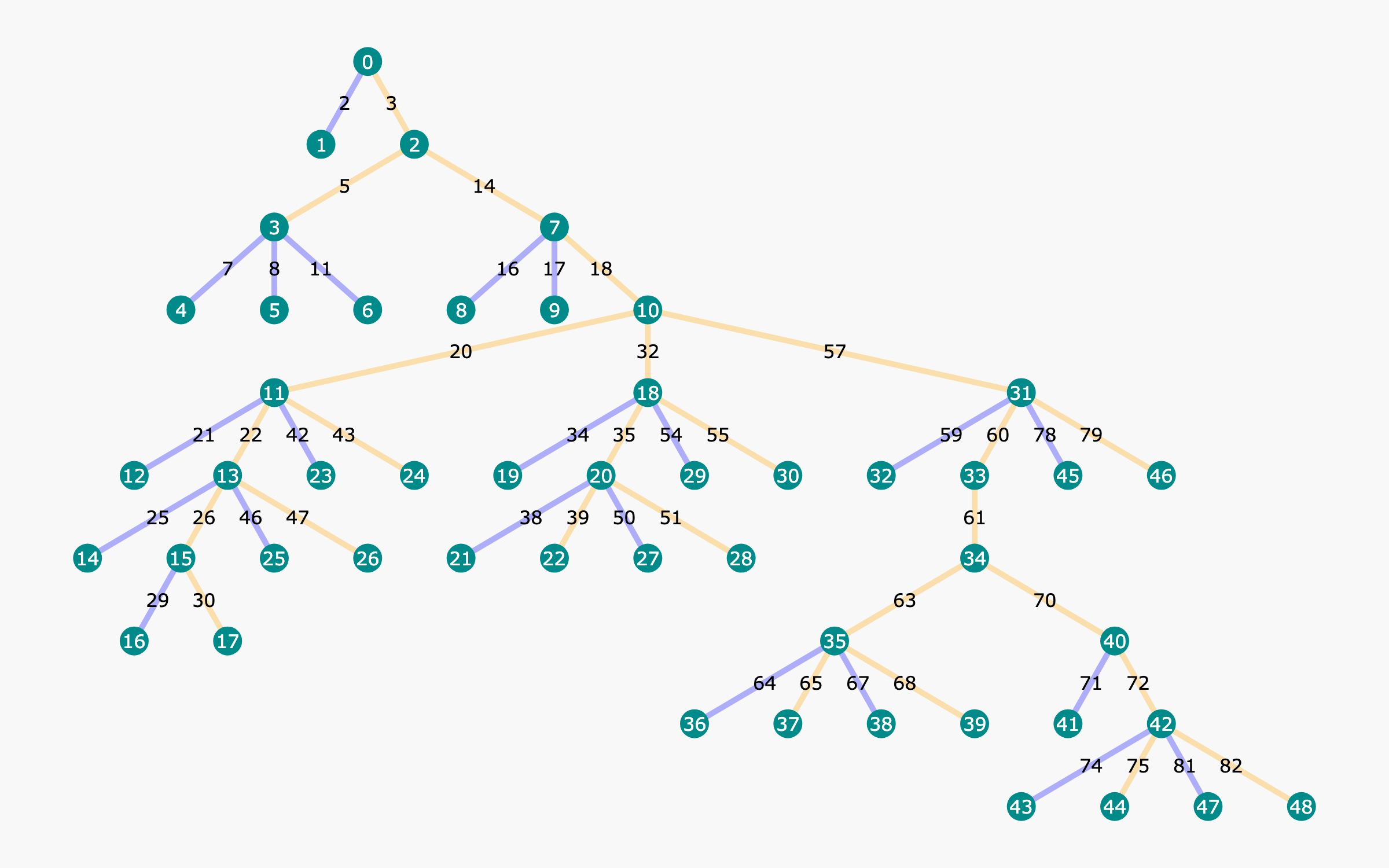
Figure 1: Example tree structure built with our proposed OmegaPRM algorithm. Each node in the tree indicates a state of partial chain-of-thought solution, with information including accuracy of rollouts and other statistics. Each edge indicates an action, i.e., a reasoning step, from the last state. Yellow edges are correct steps and blue edges are wrong.
Beyond prompting and further training, developing effective decoding strategies is another crucial avenue for improvement. Self-consistency decoding (Wang et al., 2023) leverages multiple reasoning paths to arrive at a voted answer. Incorporating a verifier, such as an off-the-shelf LLM (Huang et al., 2022; Luo et al., 2023), can further guide LLMs in reasoning tasks by providing a feedback loop to verify final answers, identify errors, and suggest corrections. However, the gain of such approaches remains limited for complex multi-step reasoning problems. Reward models offer a promising alternative to verifiers, enabling the reranking of candidate outcomes based on reward signals to ensure higher accuracy. Two primary types of reward models have emerged: Outcome Reward Models (ORMs; Yu et al., 2024; Cobbe et al., 2021), which provide feedback only at the end of the problem-solving process, and Process Reward Models (PRMs; Li et al., 2023; Uesato et al., 2022; Lightman et al., 2023), which offer granular feedback at each reasoning step. PRMs have demonstrated superior effectiveness for complex reasoning tasks by providing such fine-grained supervision.
The primary bottleneck in developing PRMs lies in obtaining process supervision signals, which require supervised labels for each reasoning step. Current approaches rely heavily on costly and labor-intensive human annotation (Uesato et al., 2022; Lightman et al., 2023). Automating this process is crucial for scalability and efficiency. While recent efforts using per-step Monte Carlo estimation have shown promise (Wang et al., 2024a, b), their efficiency remains limited due to the vast search space. To address this challenge, we introduce OmegaPRM, a novel divide-and-conquer Monte Carlo Tree Search (MCTS) algorithm inspired by AlphaGo Zero (Silver et al., 2017) for automated process supervision data collection. For each question, we build a Monte Carlo Tree, as shown in Fig. 1, with the details explained in Section 3.3. This algorithm enables efficient collection of over 1.5 million high-quality process annotations without human intervention. Our PRM, trained on this dataset and combined with weighted self-consistency decoding, significantly improves the performance of instruction-tuned Gemini Pro from 51% to 69.4% on MATH500 (Lightman et al., 2023) and from 86.4% to 93.6% on GSM8K (Cobbe et al., 2021). We also boosted the success rates of Gemma2 27B from 42.3% to 58.2% on MATH500 and from 74.0% to 92.2% on GSM8K.
Our main contributions are as follows:
- We propose a novel divide-and-conquer style Monte Carlo Tree Search algorithm for automated process supervision data generation.
- The algorithm enables the efficient generation of over 1.5 million process supervision annotations, representing the largest and highest quality dataset of its kind to date. Additionally, the entire process operates without any human annotation, making our method both financially and computationally cost-effective.
- We combine our verifier with weighted self-consistency to further boost the performance of LLM reasoning. We significantly improves the success rates from 51% to 69.4% on MATH500 and from 86.4% to 93.6% on GSM8K for instruction-tuned Gemini Pro. For Gemma2 27B, we also improved the success rates of from 42.3% to 58.2% on MATH500 and from 74.0% to 92.2% on GSM8K.
## 2 Related Work
#### Improving mathematical reasoning ability of LLMs.
Mathematical reasoning poses significant challenges for LLMs, and it is one of the key tasks for evaluating the reasoning ability of LLMs. With a huge amount of math problems in pretraining datasets, the pretrained LLMs (OpenAI, 2023; Gemini Team et al., 2024; Touvron et al., 2023) are able to solve simple problems, yet struggle with more complicated reasoning. To overcome that, the chain-of-thought (Wei et al., 2022b; Fu et al., 2023) type prompting algorithms were proposed. These techniques were effective in improving the performance of LLMs on reasoning tasks without modifying the model parameters. The performance was further improved by supervised fine-tuning (SFT; Cobbe et al., 2021; Liu et al., 2024; Yu et al., 2023) with high quality question-response pairs with full CoT reasoning steps.
#### Application of reward models in mathematical reasoning of LLMs.
To further improve the LLM’s math reasoning performance, verifiers can help to rank and select the best answer when multiple rollouts are available. Several works (Huang et al., 2022; Luo et al., 2023) have shown that using LLM as verifier is not suitable for math reasoning. For trained verifiers, two types of reward models are commonly used: Outcome Reward Model (ORM) and Process Reward Model (PRM). Both have shown performance boost on math reasoning over self-consistency (Cobbe et al., 2021; Uesato et al., 2022; Lightman et al., 2023), yet evidence has shown that PRM outperforms ORM (Lightman et al., 2023; Wang et al., 2024a). Generating high quality process supervision data is the key for training PRM, besides expensive human annotation (Lightman et al., 2023), Math-Shepherd (Wang et al., 2024a) and MiPS (Wang et al., 2024b) explored Monte Carlo estimation to automate the data collection process with human involvement, and both observed large performance gain. Our work shared the essence with MiPS and Math-Shepherd, but we explore further in collecting the process data using MCTS.
#### Monte Carlo Tree Search (MCTS).
MCTS (Świechowski et al., 2021) has been widely adopted in reinforcement learning (RL). AlphaGo (Silver et al., 2016) and AlphaGo Zero (Silver et al., 2017) were able to achieve great performance with MCTS and deep reinforcement learning. For LLMs, there are planning algorithms that fall in the category of tree search, such as Tree-of-Thought (Yao et al., 2023) and Reasoning-via-Planing (Hao et al., 2023). Recently, utilizing tree-like decoding to find the best output during the inference-time has become a hot topic to explore as well, multiple works (Feng et al., 2023; Ma et al., 2023; Zhang et al., 2024; Tian et al., 2024; Feng et al., 2024; Kang et al., 2024) have observed improvements in reasoning tasks.
## 3 Methods
### 3.1 Process Supervision
Process supervision is a concept proposed to differentiate from outcome supervision. The reward models trained with these objectives are termed Process Reward Models (PRMs) and Outcome Reward Models (ORMs), respectively. In the ORM framework, given a query $q$ (e.g., a mathematical problem) and its corresponding response $x$ (e.g., a model-generated solution), an ORM is trained to predict the correctness of the final answer within the response. Formally, an ORM takes $q$ and $x$ and outputs the probability $p=\mathrm{ORM}(q,x)$ that the final answer in the response is correct. With a training set of question-answer pairs available, an ORM can be trained by sampling outputs from a policy model (e.g., a pretrained or fine-tuned LLM) using the questions and obtaining the correctness labels by comparing these outputs with the golden answers.
In contrast, a PRM is trained to predict the correctness of each intermediate step $x_{t}$ in the solution. Formally, $p_{t}=\mathrm{PRM}([q,x_{1:t-1}],x_{t})$ , where $x_{1:i}=[x_{1},\ldots,x_{i}]$ represents the first $i$ steps in the solution. This provides more precise and fine-grained feedback than ORMs, as it identifies the exact location of errors. Process supervision has also been shown to mitigate incorrect reasoning in the domain of mathematical problem solving. Despite these advantages, obtaining the intermediate signal for each step’s correctness to train such a PRM is non-trivial. Previous work (Lightman et al., 2023) has relied on hiring domain experts to manually annotate the labels, which is and difficult to scale.
### 3.2 Process Annotation with Monte Carlo Method
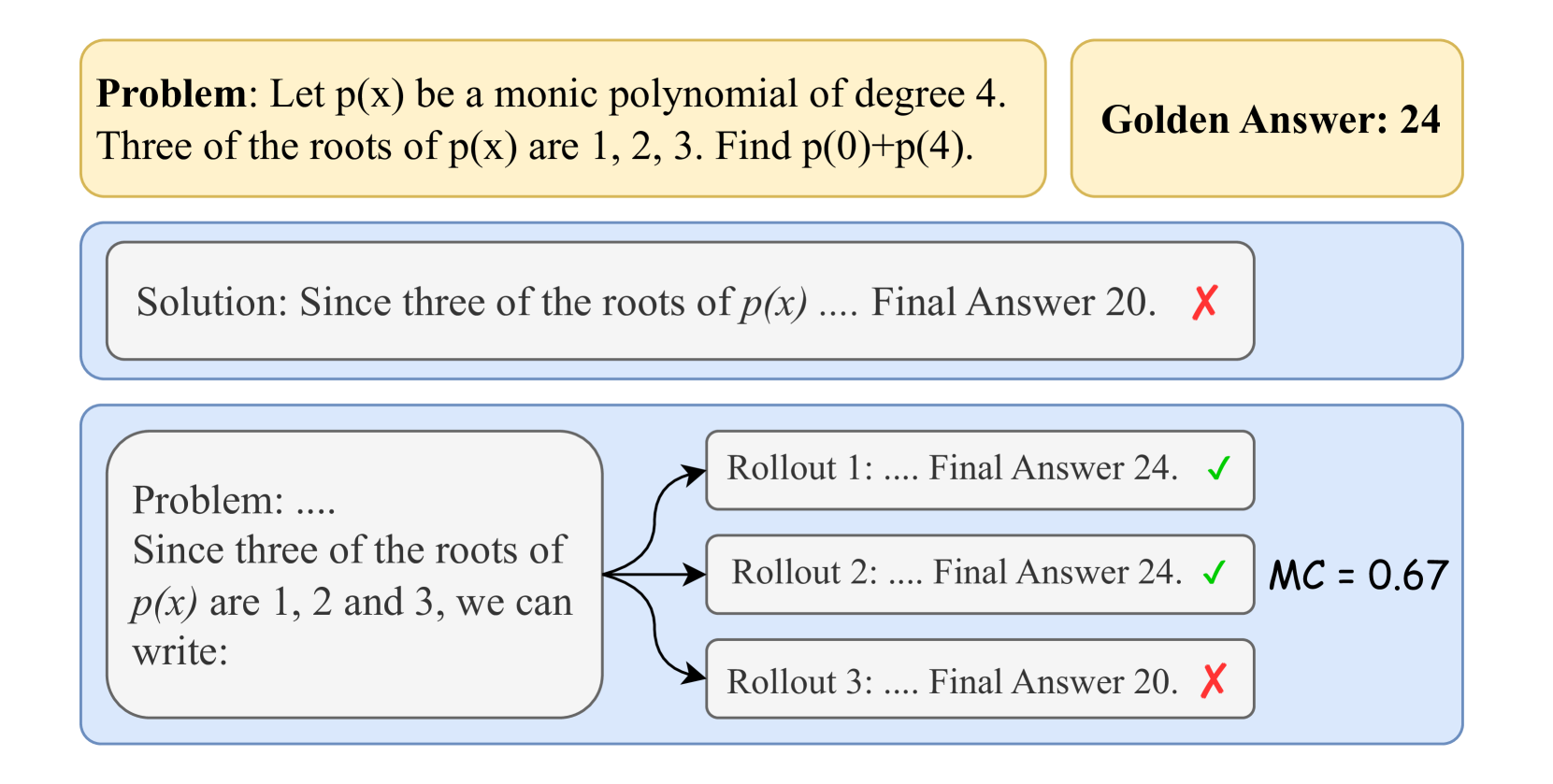
In two closely related works, Math-Shepherd (Wang et al., 2024a) and MiPS (Wang et al., 2024b), the authors propose an automatic annotation approach to obtain process supervision signals using the Monte Carlo method. Specifically, a “completer” policy is established that can take a question $q$ and a prefix solution comprising the first $t$ steps $x_{1:t}$ and output the completion — often referred to as a “rollout” in reinforcement learning — of the subsequent steps until the final answer is reached. As shown in Fig. 2 (a), for any step of a solution, the completer policy can be used to randomly sample $k$ rollouts from that step. The final answers of these rollouts are compared to the golden answer, providing $k$ labels of answer correctness corresponding to the $k$ rollouts. Subsequently, the ratio of correct rollouts to total rollouts from the $t$ -th step, as represented in Eq. 1, estimates the “correctness level” of the prefix steps up to $t$ . Regardless of false positives, $x_{1:t}$ should be considered correct as long as any of the rollouts is correct in the logical reasoning scenario.
$$
c_{t}=\mathrm{MonteCarlo}(q,x_{1:t})=\frac{\mathrm{num}(\text{correct rollouts
from $t$-th step})}{\mathrm{num}(\text{total rollouts from $t$-th step})} \tag{1}
$$
Taking a step forward, a straightforward strategy to annotate the correctness of intermediate steps in a solution is to perform rollouts for every step from the beginning to the end, as done in both Math-Shepherd and MiPS. However, this brute-force approach requires a large number of policy calls. To optimize annotation efficiency, we propose a binary-search-based Monte Carlo estimation.
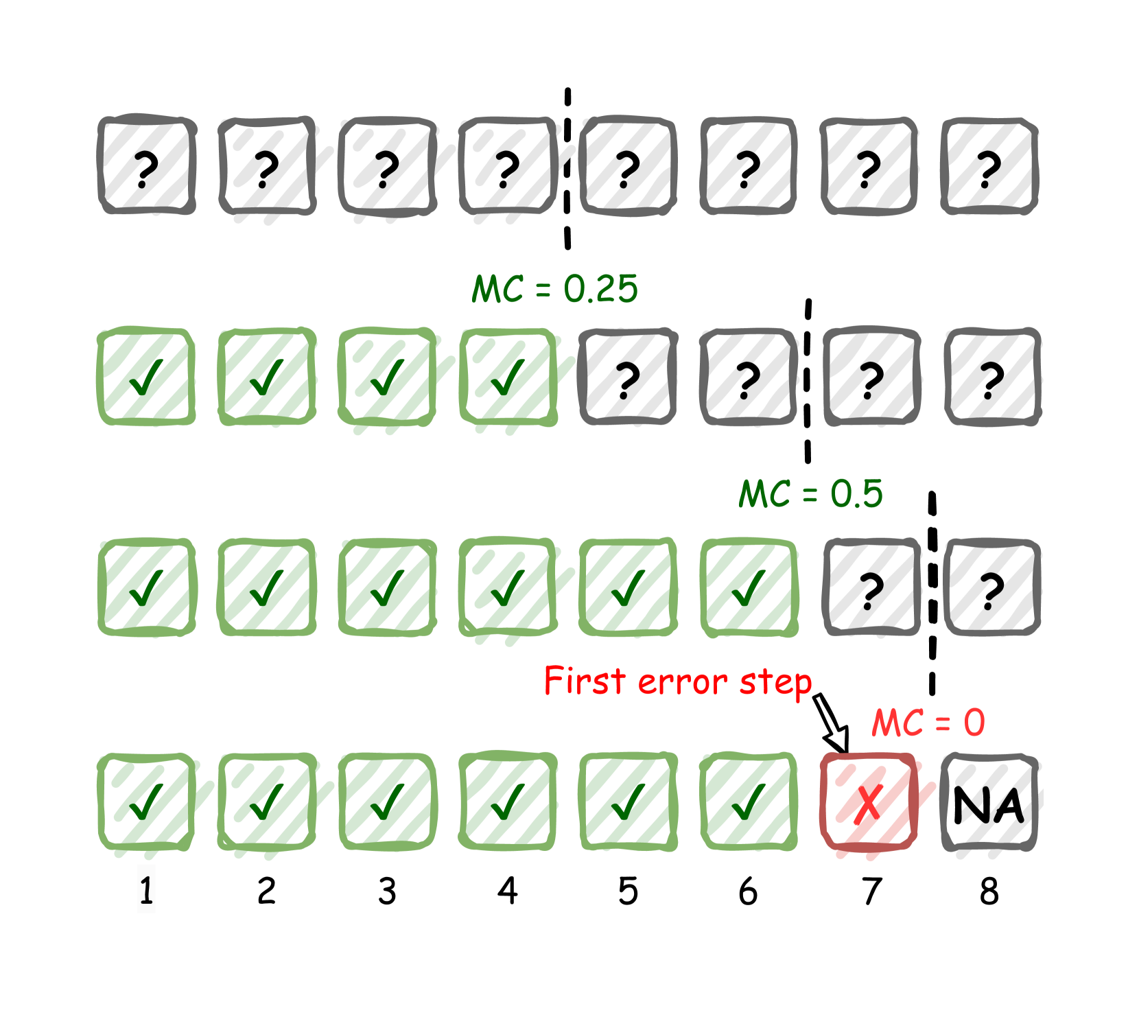
Monte Carlo estimation using binary search. As suggested by Lightman et al. (2023), supervising up to the first incorrect step in a solution is sufficient to train a PRM. Therefore, our objective is locating the first error in an efficient way. We achieve this by repeatedly dividing the solution and performing rollouts. Assuming no false positives or negatives, we start with a solution with potential errors and split it at the midpoint $m$ . We then perform rollouts for $s_{1:m}$ with two possible outcomes: (1) $c_{m}>0$ , indicating that the first half of the solution is correct, as at least one correct answer can be rolled out from $m$ -th step, and thus the error is in the second half; (2) $c_{m}=0$ , indicating the error is very likely in the first half, as none of the rollouts from $m$ -th step is correct. This process narrows down the error location to either the first or second half of the solution. As shown in Fig. 2 (b), by repeating this process on the erroneous half iteratively until the partial solution is sufficiently small (i.e., short enough to be considered as a single step), we can locate the first error with a time complexity of $O(k\log M)$ rather than $O(kM)$ in the brute-force setting, where $M$ is the total number of steps in the original solution.
### 3.3 Monte Carlo Tree Search
Although binary search improves the efficiency of locating the first error in a solution, we are still not fully utilizing policy calls as rollouts are simply discarded after stepwise Monte Carlo estimation. In practice, it is necessary to collect multiple PRM training examples (a.k.a., triplets of question, partial solution and correctness label) for a question (Lightman et al., 2023; Wang et al., 2024a). Instead of starting from scratch each time, we can store all rollouts during the process and conduct binary searches from any of these rollouts whenever we need to collect a new example. This approach allows for triplets with the same solution prefix but different completions and error locations. Such reasoning structures can be represented as a tree, as described in previous work like Tree of Thought (Yao et al., 2023).
Formally, consider a state-action tree representing detailed reasoning paths for a question, where a state $s$ contains the question and all preceding reasoning steps, and an action $a$ is a potential subsequent step from a specific state. The root state is the question without any reasoning steps: $r_{\text{root}}=q$ . The policy can be directly modeled by a language model as $\pi(a|s)=\mathrm{LM}(a|s)$ , and the state transition function is simply the concatenation of the preceding steps and the action step, i.e., $s^{\prime}=\mathrm{Concatenate}(s,a)$ .
Collecting PRM training examples for a question can now be formulated as constructing such a state-action tree. This reminds us the classic Monte Carlo Tree Search (MCTS) algorithm, which has been successful in many deep reinforcement learning applications (Silver et al., 2016, 2017). However, there are some key differences when using a language model as the policy. First, MCTS typically handles an environment with a finite action space, such as the game of Go, which has fewer than $361$ possible actions per state (Silver et al., 2017). In contrast, an LM policy has an infinite action space, as it can generate an unlimited number of distinct actions (sequences of tokens) given a prompt. In practice, we use temperature sampling to generate a fix number of $k$ completions for a prompt, treating the group of $k$ actions as an approximate action space. Second, an LM policy can sample a full rollout until the termination state (i.e., reaching the final answer) without too much overhead than generating a single step, enabling the possibility of binary search. Consequently, we propose an adaptation of the MCTS algorithm named OmegaPRM, primarily based on the one introduced in AlphaGo (Silver et al., 2016), but with modifications to better accommodate the scenario of PRM training data collection. We describe the algorithm details as below.
#### Tree Structure.
Each node $s$ in the tree contains the question $q$ and prefix solution $x_{1:t}$ , together with all previous rollouts $\{(s,r_{i})\}_{i=1}^{k}$ from the state. Each edge $(s,a)$ is either a single step or a sequence of consecutive steps from the node $s$ . The nodes also store a set of statistics,
$$
\{N(s),\mathrm{MC}(s),Q(s,r)\},
$$
where $N(s)$ denotes the visit count of a state, $\mathrm{MC}(s)$ represents the Monte Carlo estimation of a state as specified in Eq. 1, and $Q(s,r)$ is a state-rollout value function that is correlated to the chance of selecting a rollout during the selection phase of tree traversal. Specifically,
<details>
<summary>x1.png Details</summary>
### Visual Description
## Diagram: Mathematical Problem Solving with Multiple Rollouts
### Overview
The image is a diagram illustrating a mathematical problem, one incorrect solution attempt, and a process of generating multiple solution attempts ("rollouts") with varying correctness. It includes the problem statement, a "Golden Answer," an incorrect solution, and a branching diagram showing three rollouts with a final accuracy metric.
### Components/Axes
The diagram is structured into three main horizontal sections against a light gray background.
1. **Top Section (Yellow Boxes):**
* **Left Box (Problem Statement):** Contains the text: "Problem: Let p(x) be a monic polynomial of degree 4. Three of the roots of p(x) are 1, 2, 3. Find p(0)+p(4)."
* **Right Box (Golden Answer):** Contains the text: "Golden Answer: 24"
2. **Middle Section (Blue Box with Incorrect Solution):**
* A single rounded rectangle containing the text: "Solution: Since three of the roots of p(x) .... Final Answer 20." A red "X" symbol is placed to the right of the text, indicating this answer is incorrect.
3. **Bottom Section (Blue Box with Rollout Diagram):**
* **Left Component (Problem Restatement):** A rounded rectangle containing the text: "Problem: .... Since three of the roots of p(x) are 1, 2 and 3, we can write:"
* **Right Components (Rollout Boxes):** Three separate rounded rectangles, each connected by an arrow originating from the left component.
* **Rollout 1 (Top):** Text: "Rollout 1: .... Final Answer 24." Followed by a green checkmark (✓).
* **Rollout 2 (Middle):** Text: "Rollout 2: .... Final Answer 24." Followed by a green checkmark (✓).
* **Rollout 3 (Bottom):** Text: "Rollout 3: .... Final Answer 20." Followed by a red "X".
* **Metric Label:** To the right of the three rollout boxes, the text "MC = 0.67" is displayed.
### Detailed Analysis
* **Problem:** The core task is to evaluate the expression `p(0) + p(4)` for a monic (leading coefficient of 1) degree-4 polynomial `p(x)`, given that three of its roots are 1, 2, and 3.
* **Golden Answer:** The provided correct answer is **24**.
* **Incorrect Solution:** A single solution attempt shown in the middle section concludes with "Final Answer 20," which is marked as incorrect.
* **Rollout Process:** The bottom diagram shows a process where the problem is restated, leading to three independent solution attempts ("rollouts").
* **Rollout 1 & 2:** Both correctly arrive at the answer **24** (marked with ✓).
* **Rollout 3:** Incorrectly arrives at the answer **20** (marked with X).
* **Performance Metric:** The label "MC = 0.67" is positioned to the right of the rollouts. Given the context of multiple attempts, "MC" likely stands for "Monte Carlo" or a similar confidence/agreement metric. The value 0.67 corresponds to the proportion of correct rollouts (2 out of 3).
### Key Observations
1. **Discrepancy in Answers:** There is a clear conflict between the "Golden Answer" (24) and the answer from the single incorrect solution (20). The rollout process demonstrates that both answers can be generated by the underlying system.
2. **Majority Correctness:** The rollout diagram shows that the correct answer (24) is produced more frequently (2 out of 3 times) than the incorrect answer (20).
3. **Metric Calculation:** The "MC = 0.67" metric directly quantifies the agreement or confidence based on the rollout results, calculated as 2/3 ≈ 0.67.
4. **Visual Coding:** Correctness is consistently indicated by green checkmarks (✓) and incorrectness by red "X" symbols throughout the diagram.
### Interpretation
This diagram appears to visualize the output of a **probabilistic or sampling-based problem-solving system**, such as a large language model using techniques like self-consistency or Monte Carlo tree search. The system generates multiple reasoning paths ("rollouts") for the same problem.
* **What it demonstrates:** The system is not deterministic; it can produce different final answers for the same input. The "Golden Answer" serves as the ground truth. The diagram shows that while the system can produce the correct answer, it is also susceptible to generating a specific incorrect answer (20).
* **How elements relate:** The top section establishes the problem and ground truth. The middle section shows a single failure case. The bottom section provides a more robust analysis by showing the distribution of outcomes from multiple attempts, culminating in a summary metric (MC=0.67) that reflects the system's confidence or reliability for this specific problem.
* **Notable implication:** The value "MC = 0.67" suggests that for this problem, the system has a ~67% chance of producing the correct answer in a single rollout, based on this sample of three. This highlights the importance of using multiple sampling and aggregation methods (like majority voting) to improve reliability in AI-based problem-solving, rather than relying on a single output. The specific incorrect answer "20" may point to a common logical or computational pitfall in the solution process for this polynomial problem.
</details>
(a) Monte Carlo estimation of a prefix solution.
<details>
<summary>x2.png Details</summary>
### Visual Description
## Diagram: MC (Margin of Confidence) Progression and Error Impact
### Overview
The image is a conceptual diagram illustrating the progression of a metric labeled "MC" (likely "Margin of Confidence" or a similar measure) across a sequence of 8 steps or trials. It visually demonstrates how MC changes based on the accumulation of correct outcomes (checkmarks) and is reset to zero upon the occurrence of a first error (red X). The diagram uses a hand-drawn, sketched aesthetic with boxes, symbols, and annotations.
### Components/Axes
* **Structure:** Four horizontal rows, each containing a sequence of 8 boxes.
* **Box States:**
* **Question Mark (`?`):** Grey box with a black question mark. Represents an unknown, pending, or unattempted step.
* **Checkmark (`✓`):** Green box with a green checkmark. Represents a correct or successful step.
* **Red X (`X`):** Red box with a red "X". Represents an incorrect or failed step.
* **NA:** Grey box with the text "NA". Represents a step that is "Not Applicable" or cannot be evaluated.
* **Annotations:**
* **MC Values:** Green text (`MC = 0.25`, `MC = 0.5`) and red text (`MC = 0`) placed above specific rows.
* **Dashed Vertical Lines:** Black dashed lines separating groups of boxes within a row, indicating a threshold or point of evaluation.
* **"First error step" Label:** Red text with an arrow pointing to the red "X" in the bottom row.
* **Step Numbers:** Black numbers (1 through 8) below the boxes in the bottom row, labeling the sequence position.
* **Spatial Layout:**
* The four rows are stacked vertically.
* The dashed line in the first row is positioned after the 4th box.
* The dashed line in the second row is positioned after the 6th box.
* The dashed line in the third row is positioned after the 7th box.
* The "MC = 0.25" label is centered above the second row.
* The "MC = 0.5" label is centered above the third row.
* The "MC = 0" label and "First error step" annotation are positioned above the 7th box of the bottom row.
### Detailed Analysis
The diagram presents a sequence of four scenarios or states, progressing from top to bottom.
1. **Row 1 (Top):**
* **Content:** 8 boxes, all containing question marks (`?`).
* **Annotation:** A dashed vertical line is placed after the 4th box.
* **MC Value:** No explicit MC value is given for this row.
* **Interpretation:** This represents the initial state where no steps have been attempted or evaluated.
2. **Row 2:**
* **Content:** The first 4 boxes contain checkmarks (`✓`). Boxes 5-8 contain question marks (`?`).
* **Annotation:** A dashed vertical line is placed after the 6th box.
* **MC Value:** `MC = 0.25` (green text).
* **Trend:** The MC value is associated with having 4 correct steps out of the first 6 positions (as indicated by the dashed line). The calculation is not explicitly shown, but 4/6 ≈ 0.67, not 0.25. This suggests MC may be a more complex metric (e.g., confidence margin) rather than a simple accuracy ratio.
3. **Row 3:**
* **Content:** The first 6 boxes contain checkmarks (`✓`). Boxes 7-8 contain question marks (`?`).
* **Annotation:** A dashed vertical line is placed after the 7th box.
* **MC Value:** `MC = 0.5` (green text).
* **Trend:** The MC value has increased from 0.25 to 0.5 as the number of consecutive correct steps increased from 4 to 6. The evaluation point (dashed line) has also moved one step to the right.
4. **Row 4 (Bottom):**
* **Content:** Boxes 1-6 contain checkmarks (`✓`). Box 7 contains a red "X". Box 8 contains "NA".
* **Step Labels:** Numbers 1 through 8 are placed below the boxes.
* **Annotations:** A red arrow labeled "First error step" points to the red "X" in box 7. The text `MC = 0` (red) is placed above this box.
* **Trend:** The sequence of correct steps is broken at step 7. The MC value drops to 0 immediately upon the first error. Step 8 is marked "NA", implying the process terminates or the metric is undefined after a failure.
### Key Observations
1. **MC is Reset by Error:** The most critical observation is that a single error (the red "X" at step 7) causes the MC value to drop to zero (`MC = 0`), regardless of the prior streak of correct answers.
2. **MC Increases with Success:** In the error-free scenarios (Rows 2 and 3), the MC value increases (from 0.25 to 0.5) as the number of consecutive correct steps increases.
3. **Evaluation Point Shifts:** The dashed vertical line, which likely marks the point at which MC is calculated, moves to the right as more steps are completed correctly (from after step 4, to after step 6, to after step 7).
4. **Termination on Failure:** The "NA" in the final box of the bottom row suggests that the process or metric calculation stops after an error occurs.
5. **Non-Linear MC Calculation:** The MC values (0.25 for 4/6 correct, 0.5 for 6/7 correct) do not correspond directly to the proportion of correct steps, indicating it is a derived metric, possibly a confidence score or margin.
### Interpretation
This diagram is a pedagogical tool explaining the behavior of a sequential evaluation metric, likely used in fields like machine learning (e.g., reinforcement learning, confidence calibration), quality control, or testing protocols.
* **What it Demonstrates:** It illustrates a "streak-based" or "consecutive success" confidence model. The system's confidence (MC) builds gradually with each correct outcome but is fragile—a single failure completely resets confidence to zero. This models a strict, perhaps conservative, evaluation where reliability is defined by perfect performance up to a point.
* **Relationship Between Elements:** The rows show a temporal progression. The dashed line represents the "current evaluation point." The MC value is a function of the history of outcomes *up to that point*. The final row shows the catastrophic effect of an error on this specific metric.
* **Notable Implications:**
* **Fragility:** The metric is highly sensitive to the most recent outcome. A long history of success is invalidated by one mistake.
* **All-or-Nothing:** It suggests a system where partial success is not valued; only perfect sequences contribute to a positive MC.
* **Process Termination:** The "NA" implies that after a failure, the subsequent step may not be attempted or the metric is no longer meaningful, highlighting a potential stopping condition in the underlying process.
In essence, the diagram argues for a specific, stringent definition of confidence or reliability where it is earned incrementally but lost instantly.
</details>
(b) Error locating using binary search.
<details>
<summary>x3.png Details</summary>
### Visual Description
## Diagram: Three-Phase Tree Algorithm Illustration
### Overview
The image is a technical diagram illustrating three sequential or related operations on a tree data structure. The operations are labeled "Select", "Binary Search", and "Maintain", each depicted as a separate tree diagram arranged horizontally from left to right. The diagram uses visual cues like node color, edge style, and annotations to convey the state and actions at each phase.
### Components/Axes
The diagram consists of three distinct tree structures, each with the following common components:
* **Nodes:** Represented as circles containing numerical identifiers (0, 1, 2, 3, 4, 5, 6).
* **Edges:** Lines connecting nodes, with different styles indicating different relationships or states.
* **Labels:** Textual annotations describing the operation phase and specific node states.
* **Color Coding:** Nodes are colored in two shades of teal/green. A darker teal is used for "active" or "selected" nodes in the first and third diagrams, while a lighter teal is used for nodes in the middle diagram.
**Legend (Inferred from visual patterns):**
* **Node Fill Color:**
* Dark Teal: Active/Selected node (Diagrams 1 & 3).
* Light Teal: Inactive/Unselected node (Diagram 2).
* **Edge Style:**
* Solid Purple Line: Primary or confirmed parent-child connection.
* Dashed Yellow Line: Secondary or potential connection.
* Dotted Black Line: Potential future paths or unexplored branches (only in Diagram 1).
* **Text Annotations:**
* Red Text ("Selected"): Highlights the chosen node in Diagram 1.
* Black Text ("N++", "MC, Q"): Indicates operations or properties associated with nodes in Diagram 3.
### Detailed Analysis
#### **Diagram 1: "Select" (Left)**
* **Title:** "Select" (centered above the tree).
* **Tree Structure:** A root node (0) with two children (1 and 3). Node 1 has a child (2). Dotted lines extend from nodes 0, 1, 2, and 3, suggesting potential but unexplored branches.
* **Key Action:** Node 0 is filled with dark teal. A red arrow points to it with the label **"Selected"** in red text, positioned to the upper-right of node 0.
* **Spatial Grounding:** The "Selected" annotation is in the top-right quadrant of this sub-diagram. The dotted lines radiate downwards and outwards from the existing nodes.
#### **Diagram 2: "Binary Search" (Center)**
* **Title:** "Binary Search" (centered above the tree).
* **Tree Structure:** The same underlying tree topology as Diagram 1, but with different node states and a highlighted path.
* **Node States:** All nodes (0, 1, 2, 3, 4, 5, 6) are filled with light teal, indicating they are not the primary focus of selection.
* **Highlighted Path:** A specific path is emphasized:
* From root **0** to child **4** via a **dashed yellow line**.
* From node **4** to child **5** via a **dashed yellow line**.
* From node **5** to child **6** via a **solid purple line**.
* **Trend Verification:** The visual trend shows a search path descending from the root (0) down the rightmost branch (0 -> 4 -> 5 -> 6), with the final connection being solid.
#### **Diagram 3: "Maintain" (Right)**
* **Title:** "Maintain" (centered above the tree).
* **Tree Structure:** Identical topology to the previous diagrams.
* **Node States:** Nodes 0, 1, 2, 3, 4, 5, and 6 are all filled with dark teal, indicating they are all active or have been updated.
* **Annotations:**
* To the right of root node **0**: The text **"N++"**.
* To the right of node **4**: The text **"MC, Q"**.
* To the right of node **5**: The text **"MC, Q"**.
* To the right of node **6**: The text **"MC, Q"**.
* **Edge Styles:** The edge from 0 to 4 is dashed yellow. The edge from 4 to 5 is dashed yellow. The edge from 5 to 6 is solid purple. The edge from 0 to 1 is dashed yellow. The edge from 1 to 2 is solid purple. The edge from 0 to 3 is dashed yellow.
### Key Observations
1. **Consistent Topology:** The underlying tree structure (parent-child relationships) is identical across all three diagrams, showing the same set of nodes and connections.
2. **State Progression:** The diagrams show a clear progression: a node is **selected** (Diagram 1), a **search path** is executed (Diagram 2), and then the tree is **updated/maintained** (Diagram 3), with annotations suggesting increments ("N++") and other operations ("MC, Q").
3. **Path Consistency:** The path highlighted in the "Binary Search" phase (0->4->5->6) corresponds to the rightmost branch of the tree. The "Maintain" phase shows this same path (0->4->5->6) with consistent edge styles, but now all nodes are active.
4. **Annotation Specificity:** The "MC, Q" annotation is applied only to nodes 4, 5, and 6—the nodes along the search path from the "Binary Search" phase. The "N++" annotation is applied only to the root node (0).
### Interpretation
This diagram illustrates a three-step algorithm for operating on a tree, likely related to **dynamic tree data structures** (e.g., Link/Cut Trees, Euler Tour Trees) used in advanced algorithms for network flow, connectivity, or dynamic graph problems.
* **"Select" Phase:** Represents choosing a specific node (node 0) as the root of a preferred path or the entry point for an operation. The dotted lines suggest the algorithm considers potential paths from this node.
* **"Binary Search" Phase:** Depicts a search or access operation along a specific path in the tree (0->4->5->6). The use of "Binary Search" as a label is metaphorical, implying a hierarchical search process within the tree structure rather than a literal binary search on a sorted array. The path is likely a "preferred path" in the data structure.
* **"Maintain" Phase:** Shows the state after the operation, where the tree's metadata is updated. "N++" at the root suggests an increment of a size or counter property for the entire tree. "MC, Q" on the nodes of the accessed path (4, 5, 6) likely stands for updating properties like **M**ax **C**apacity, **Q**ueue information, or other aggregate values that must be maintained along the path after an access or modification.
**Overall Purpose:** The diagram visually explains how an operation (starting with selection) triggers a search along a specific path, which in turn necessitates updates to node and path metadata to maintain the invariants of the data structure. It emphasizes the link between path access and the maintenance of aggregated information in tree-based algorithms.
</details>
(c) Three stages in an iteration of the MCTS process.
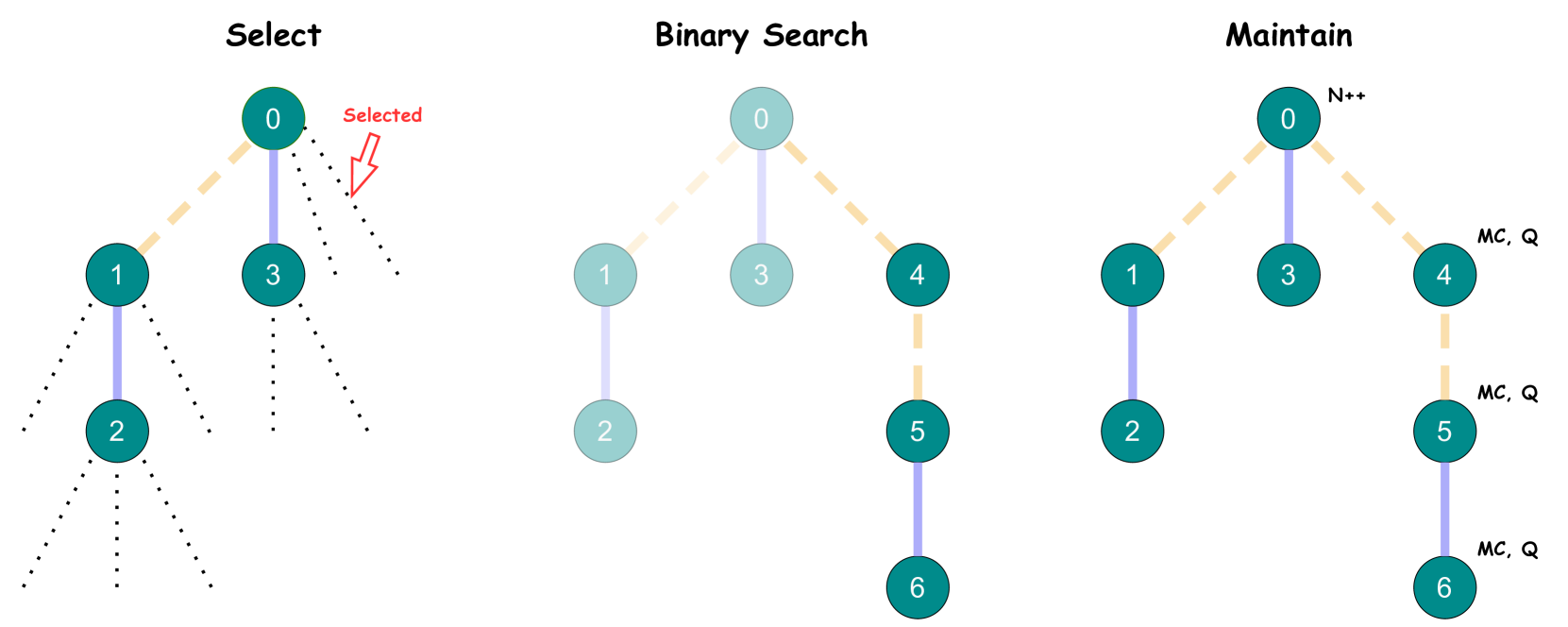
Figure 2: Illustration of the process supervision rollouts, Monte Carlo estimation using binary search and the MCTS process. (a) An example of Monte Carlo estimation of a prefix solution. Two out of the three rollouts are correct, producing the Monte Carlo estimation $\mathrm{MC}(q,x_{1:t})=2/3\approx 0.67$ . (b) An example of error locating using binary search. The first error step is located at the $7^{\text{th}}$ step after three divide-and-rollouts, where the rollout positions are indicated by the vertical dashed lines. (c) The MCTS process. The dotted lines in Select stage represent the available rollouts for binary search. The bold colored edges represent steps with correctness estimations. The yellow color indicates a correct step, i.e., with a preceding state $s$ that $\mathrm{MC}(s)>0$ and the blue color indicates an incorrect step, i.e., with $\mathrm{MC}(s)=0$ . The number of dashes in each colored edge indicates the number of steps.
$$
Q(s,r)=\alpha^{1-\mathrm{MC}(s)}\cdot\beta^{\frac{\mathrm{len}(r)}{L}}, \tag{2}
$$
where $\alpha,\beta\in(0,1]$ and $L>0$ are constant hyperparameters; while $\mathrm{len}(r)$ denotes the length of a rollout in terms of number of tokens. $Q$ is supposed to indicate how likely a rollout will be chosen for each iteration and our goal is to define a heuristic that selects the most valuable rollout to search with. The most straightforward strategy is uniformly choosing rollout candidates generated by the policy in previous rounds; however, this is obviously not an effective way. Lightman et al. (2023) suggests surfacing the convincing wrong-answer solutions for annotators during labeling. Inspired by this, we propose to prioritize supposed-to-be-correct wrong-answer rollouts during selection. We use the term supposed-to-be-correct to refer to the state with a Monte Carlo estimation $\mathrm{MC}(s)$ closed to $1$ ; and use wrong-answer to refer that the specific rollout $r$ has a wrong final answer. The rollout contains mistakes made by the policy that should have been avoided given its high $\mathrm{MC}(s)$ . We expect a PRM that learns to detect errors in such rollouts will be more useful in correcting the mistakes made by the policy. The first component in Eq. 2, $\alpha^{1-\mathrm{MC}(s)}$ , has a larger value as $\mathrm{MC}(s)$ is closer to $1$ . Additionally, we incorporate a length penalty factor $\beta^{\frac{\mathrm{len}(r)}{L}}$ , to penalize excessively long rollouts.
#### Select.
The selection phase in our algorithm is simpler than that of AlphaGo (Silver et al., 2016), which involves selecting a sequence of actions from the root to a leaf node, forming a trajectory with multiple states and actions. In contrast, we maintain a pool of all rollouts $\{(s_{i},r^{i}_{j})\}$ from previous searches that satisfy $0<\mathrm{MC}(s_{i})<1$ . During each selection, a rollout is popped and selected according to tree statistics, $(s,r)=\operatorname*{arg\,max}_{(s,r)}[Q(s,r)+U(s)]$ , using a variant of the PUCT (Rosin, 2011) algorithm,
$$
U(s)=c_{\text{puct}}\frac{\sqrt{\sum_{i}N(s_{i})}}{1+N(s)}, \tag{3}
$$
where $c_{\text{puct}}$ is a constant determining the level of exploration. This strategy initially favors rollouts with low visit counts but gradually shifts preference towards those with high rollout values.
#### Binary Search.
We perform a binary search to identify the first error location in the selected rollout, as detailed in Section 3.2. The rollouts with $0<\mathrm{MC}(s)<1$ during the process are added to the selection candidate pool. All divide-and-rollout positions before the first error become new states. For the example in Fig. 2 (b), the trajectory $s[q]\rightarrow s[q,x_{1:4}]\rightarrow s[q,x_{1:6}]\rightarrow s[q,x_{1:7}]$ is added to the tree after the binary search. The edges $s[q]\rightarrow s[q,x_{1:4}]$ and $s[q,x_{1:4}]\rightarrow s[q,x_{1:6}]$ are correct, with $\mathrm{MC}$ values of $0.25$ and $0.5$ , respectively; while the edge $s[q,x_{1:6}]\rightarrow s[q,x_{1:7}]$ is incorrect with $\mathrm{MC}$ value of $0 0$ .
#### Maintain.
After the binary search, the tree statistics $N(s)$ , $\mathrm{MC}(s)$ , and $Q(s,r)$ are updated. Specifically, $N(s)$ is incremented by $1$ for the selected $(s,r)$ . Both $\mathrm{MC}(s)$ and $Q(s,r)$ are updated for the new rollouts sampled from the binary search. This phase resembles the backup phase in AlphaGo but is simpler, as it does not require recursive updates from the leaf to the root.
#### Tree Construction.
By repeating the aboved process, we can construct a state-action tree as the example illustrated in Fig. 1. The construction ends either when the search count reaches a predetermined limit or when no additional rollout candidates are available in the pool.
### 3.4 PRM Training
Each edge $(s,a)$ with a single-step action in the constructed state-action tree can serve as a training example for the PRM. It can be trained using the standard classification loss
$$
\mathcal{L}_{\text{pointwise}}=\sum_{i=1}^{N}\hat{y}_{i}\log y_{i}+(1-\hat{y}_
{i})\log(1-y_{i}), \tag{4}
$$
where $\hat{y}_{i}$ represents the correctness label and $y_{i}=\mathrm{PRM}(s,a)$ is the prediction score of the PRM. Wang et al. (2024b) have used the Monte Carlo estimation as the correctness label, denoted as $\hat{y}=\mathrm{MC}(s)$ . Alternatively, Wang et al. (2024a) have employed a binary labeling approach, where $\hat{y}=\mathbf{1}[\mathrm{MC}(s)>0]$ , assigning $\hat{y}=1$ for any positive Monte Carlo estimation and $\hat{y}=0$ otherwise. We refer the former option as pointwise soft label and the latter as pointwise hard label. In addition, considering there are many cases where a common solution prefix has multiple single-step actions, we can also minimize the cross-entropy loss between the PRM predictions and the normalized pairwise preferences following the Bradley-Terry model (Christiano et al., 2017). We refer this training method as pairwise approach, and the detailed pairwise loss formula can be found in Section Appendix B.
We use the pointwise soft label when evaluating the main results in Section 4.1, and a comparion of the three objectives are discussed in Section 4.3.
## 4 Experiments
#### Data Generation.
We conduct our experiments on the challenging MATH dataset (Hendrycks et al., 2021). We use the same training and testing split as described in Lightman et al. (2023), which consists of $12$ K training examples and a subset with $500$ holdout representative problems from the original $5$ K testing examples introduced in Hendrycks et al. (2021). We observe similar policy performance on the full test set and the subset. For creating the process annotation data, we use the questions from the training split and set the search limit to $100$ per question, resulting $1.5$ M per-step process supervision annotations. To reduce the false positive and false negative noise, we filtered out questions that are either too hard or too easy for the model. Please refer to Appendix A for details. We use $\alpha=0.5$ , $\beta=0.9$ and $L=500$ for calculating $Q(s,r)$ in Eq. 2; and $c_{\text{puct}}=0.125$ in Eq. 3. We sample $k=8$ rollouts for each Monte Carlo estimation.
#### Models.
In previous studies (Lightman et al., 2023; Wang et al., 2024a, b), both proprietary models such as GPT-4 (OpenAI, 2023) and open-source models such as Llama2 (Touvron et al., 2023) were explored. In our study, we perform experiments with both proprietary Gemini Pro (Gemini Team et al., 2024) and open-source Gemma2 (Gemma Team et al., 2024) models. For Gemini Pro, we follow Lightman et al. (2023); Wang et al. (2024a) to initially fine-tune it on math instruction data, achieving an accuracy of approximately $51$ % on the MATH test set. The instruction-tuned model is then used for solution sampling. For open-source models, to maximize reproducibility, we directly use the pretrained Gemma2 27B checkpoint with the 4-shot prompt introduced in Gemini Team et al. (2024). The reward models are all trained from the pretrained checkpoints.
#### Metrics and baselines.
We evaluate the PRM-based majority voting results on GSM8K (Cobbe et al., 2021) and MATH500 (Lightman et al., 2023) using PRMs trained on different process supervision data. We choose the product of scores across all steps as the final solution score following Lightman et al. (2023), where the performance difference between product and minimum of scores was compared and the study showed the difference is minor. Baseline process supervision data include PRM800K (Lightman et al., 2023) and Math-Shepherd (Wang et al., 2024a), both publicly available. Additionally, we generate a process annotation dataset with our Gemini policy model using the brute-force approach described in Wang et al. (2024a, b), referred to as Math-Shepherd (our impl) in subsequent sections.
### 4.1 Main Results
<details>
<summary>x4.png Details</summary>
### Visual Description
## Line Chart: Performance Comparison of Problem-Solving Methods
### Overview
This line chart compares the performance of five different methods or models in solving problems. The performance is measured as the percentage of problems solved, plotted against an increasing number of solutions generated per problem. All methods show improved performance as the number of solutions increases, but their starting points and rates of improvement differ.
### Components/Axes
* **X-Axis (Horizontal):** Labeled "N = number of solutions per problems". It uses a logarithmic scale with base 2, marked at points: 2² (4), 2³ (8), 2⁴ (16), 2⁵ (32), and 2⁶ (64).
* **Y-Axis (Vertical):** Labeled "% Problems Solved". It is a linear scale ranging from 56 to 70, with major tick marks every 2 units (56, 58, 60, 62, 64, 66, 68, 70).
* **Legend:** Located in the bottom-right quadrant of the chart area. It contains five entries, each with a colored line, a unique marker, and a label:
1. **Green line with square marker:** "Majority Vote"
2. **Red line with upward-pointing triangle marker:** "+OmegaPRM"
3. **Purple line with circle marker:** "+PRM800K"
4. **Blue line with circle marker:** "+Shepherd"
5. **Dark purple/magenta line with circle marker:** "+Shepherd (ours)"
* **Data Series:** Each method is represented by a solid line connecting data points at each x-axis value. Each line is surrounded by a semi-transparent shaded band of the same color, likely representing a confidence interval or standard deviation.
### Detailed Analysis
**Trend Verification:** All five data series exhibit a clear upward, concave-down trend. The rate of improvement (slope) is steepest between N=2² and N=2³ and gradually flattens as N increases, suggesting diminishing returns.
**Data Point Extraction (Approximate Values):**
| Method | N=2² (4) | N=2³ (8) | N=2⁴ (16) | N=2⁵ (32) | N=2⁶ (64) |
| :--- | :--- | :--- | :--- | :--- | :--- |
| **+OmegaPRM (Red, Triangle)** | ~64.0% | ~66.6% | ~67.9% | ~68.7% | ~69.1% |
| **+PRM800K (Purple, Circle)** | ~63.0% | ~65.2% | ~66.7% | ~67.1% | ~67.7% |
| **+Shepherd (Blue, Circle)** | ~60.5% | ~63.4% | ~65.3% | ~66.0% | ~66.5% |
| **+Shepherd (ours) (Dark Purple/Magenta, Circle)** | ~58.0% | ~62.6% | ~65.0% | ~66.0% | ~67.1% |
| **Majority Vote (Green, Square)** | ~57.4% | ~62.8% | ~65.0% | ~66.2% | ~67.1% |
### Key Observations
1. **Consistent Leader:** The "+OmegaPRM" method consistently outperforms all others at every data point, maintaining a clear gap.
2. **Convergence at High N:** The performance of "Majority Vote," "+Shepherd (ours)," and "+Shepherd" converges significantly as N increases. At N=2⁶, the last three methods are within approximately 0.6 percentage points of each other (66.5% to 67.1%).
3. **Strongest Improvement:** The "+Shepherd (ours)" method shows the most dramatic improvement, starting at the lowest point (~58.0%) and nearly catching up to the second-tier methods by N=2⁶.
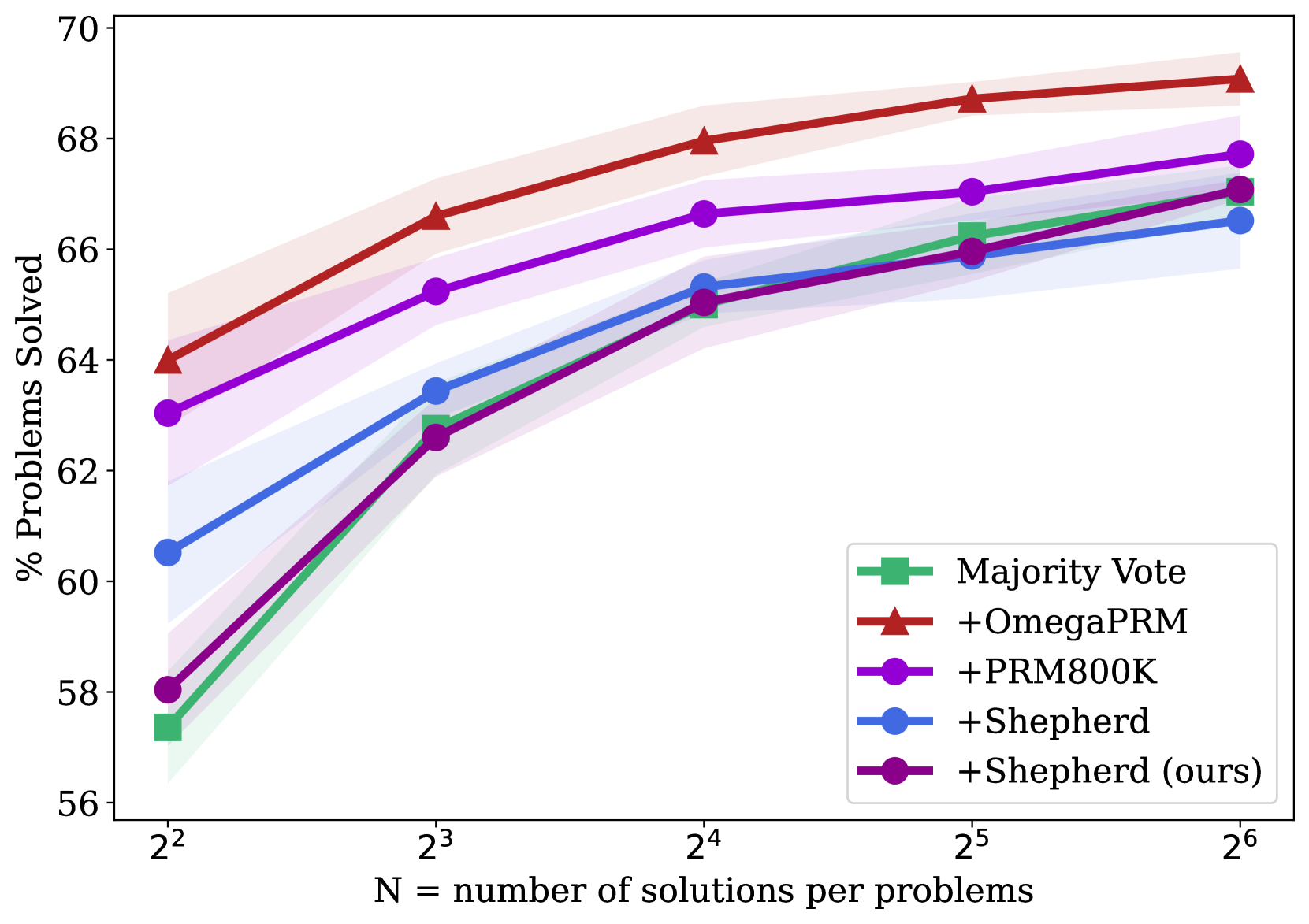
4. **Diminishing Returns:** All curves flatten noticeably after N=2⁴ (16 solutions), indicating that generating more solutions beyond this point yields progressively smaller gains in solve rate.
5. **Uncertainty Bands:** The shaded confidence intervals are wider at lower N values (especially for "+OmegaPRM" and "+PRM800K" at N=2²), suggesting greater variance in performance when fewer solutions are used. The bands narrow as N increases.
### Interpretation
The chart demonstrates the effectiveness of different techniques for improving problem-solving performance through increased sampling (generating more solutions). The data suggests that:
* **Methodology Matters Significantly:** The choice of method (e.g., +OmegaPRM vs. Majority Vote) has a larger impact on performance than simply increasing the number of solutions for lower N values. +OmegaPRM provides a substantial and consistent advantage.
* **The Value of "Ours":** The "+Shepherd (ours)" method, while starting poorly, exhibits a superior scaling law. Its steep improvement curve suggests it may be more efficient at leveraging additional solution samples, potentially making it a competitive choice at higher computational budgets (higher N).
* **Practical Trade-off:** The flattening curves highlight a key trade-off between computational cost (proportional to N) and performance gain. The optimal operating point likely lies around N=2⁴ or N=2⁵, where most of the benefit is captured before severe diminishing returns set in.
* **Baseline Comparison:** "Majority Vote," a common baseline, is outperformed by all specialized methods (+OmegaPRM, +PRM800K) at all points. It is only competitive with the Shepherd variants at high N, indicating that more sophisticated methods provide better "bang for the buck" at lower sample counts.
</details>
(a) Gemini Pro on MATH500.
<details>
<summary>x5.png Details</summary>
### Visual Description
## Line Chart: Performance Scaling with Increased Solution Sampling
### Overview
The image is a line chart comparing the performance of five different methods for solving problems, measured as the percentage of problems solved, as a function of the number of solutions sampled per problem (N). The chart demonstrates how each method's effectiveness scales with increased computational effort (more solutions). All methods show improvement as N increases, but with different starting points and rates of gain.
### Components/Axes
* **Y-Axis:** Labeled "% Problems Solved". The scale runs from 89 to 94, with major tick marks at every integer value (89, 90, 91, 92, 93, 94).
* **X-Axis:** Labeled "N = number of solutions per problems". The scale is logarithmic base 2, with tick marks at N = 2² (4), 2³ (8), 2⁴ (16), 2⁵ (32), and 2⁶ (64).
* **Legend:** Located in the bottom-right quadrant of the chart area. It contains five entries, each with a unique color and marker symbol:
1. **Majority Vote:** Green line with square markers (■).
2. **+OmegaPRM:** Red line with upward-pointing triangle markers (▲).
3. **+PRM800K:** Purple line with circle markers (●).
4. **+Shepherd:** Blue line with circle markers (●).
5. **+Shepherd (ours):** Dark purple/magenta line with circle markers (●).
* **Data Series:** Each method is represented by a solid line connecting data points at each N value. A semi-transparent shaded band of the corresponding color surrounds each line, likely indicating confidence intervals or standard deviation across multiple runs.
### Detailed Analysis
**Trend Verification & Data Points (Approximate Values):**
1. **+OmegaPRM (Red, ▲):**
* **Trend:** Consistently the top-performing method. Shows a steady, slightly decelerating upward slope.
* **Points:**
* N=4: ~92.5%
* N=8: ~93.1%
* N=16: ~93.3%
* N=32: ~93.4%
* N=64: ~93.6%
2. **+PRM800K (Purple, ●):**
* **Trend:** Second-best performance. Slopes upward, with a noticeable increase between N=4 and N=8, then a more gradual rise.
* **Points:**
* N=4: ~91.7%
* N=8: ~92.5%
* N=16: ~92.7%
* N=32: ~92.8%
* N=64: ~92.9%
3. **+Shepherd (Blue, ●):**
* **Trend:** Starts lower but shows strong improvement, nearly catching up to +PRM800K at higher N. The slope is steepest between N=4 and N=16.
* **Points:**
* N=4: ~91.1%
* N=8: ~91.9%
* N=16: ~92.6%
* N=32: ~92.7%
* N=64: ~92.7% (appears to plateau)
4. **Majority Vote (Green, ■):**
* **Trend:** Starts as the lowest-performing method at N=4 but exhibits the most dramatic relative improvement, surpassing the "+Shepherd (ours)" method.
* **Points:**
* N=4: ~89.2%
* N=8: ~90.9%
* N=16: ~91.9%
* N=32: ~92.5%
* N=64: ~92.6%
5. **+Shepherd (ours) (Dark Purple, ●):**
* **Trend:** Starts very close to Majority Vote. Improves but at a slower rate than the other methods, resulting in it being overtaken. It shows the most pronounced plateau after N=16.
* **Points:**
* N=4: ~89.1%
* N=8: ~90.7%
* N=16: ~91.6%
* N=32: ~91.8%
* N=64: ~91.8%
### Key Observations
1. **Performance Hierarchy:** A clear and consistent ranking is maintained across all N values: +OmegaPRM > +PRM800K > +Shepherd > Majority Vote ≈ +Shepherd (ours). The gap between the top method (+OmegaPRM) and the others remains significant.
2. **Diminishing Returns:** All curves show diminishing marginal returns. The performance gain from doubling N is much larger when moving from N=4 to N=8 than from N=32 to N=64.
3. **Convergence:** The performance of "+Shepherd" and "+PRM800K" converges at higher N (32, 64), becoming nearly indistinguishable within the shaded uncertainty bands.
4. **Anomaly:** The method labeled "+Shepherd (ours)" underperforms the standard "+Shepherd" method and is eventually surpassed by the simpler "Majority Vote" baseline. This suggests the "(ours)" variant may be less effective or optimized for a different objective.
5. **Uncertainty:** The shaded bands are widest at lower N values (especially for Majority Vote and +Shepherd (ours) at N=4), indicating higher variance in results when fewer solutions are sampled. The bands narrow as N increases.
### Interpretation
This chart likely comes from a research paper in machine learning or automated reasoning, comparing different methods for generating and verifying solutions to problems (e.g., mathematical reasoning, code generation). The key takeaway is that the **+OmegaPRM method is superior**, achieving the highest solve rate at every level of computational budget (N). Its advantage is established early (at N=4) and maintained.
The data demonstrates a fundamental trade-off: **more sampling (higher N) improves performance for all methods, but at a decreasing rate.** This suggests that simply throwing more computation at the problem has limits, and algorithmic improvements (like those in +OmegaPRM) are crucial for significant gains.
The underperformance of "+Shepherd (ours)" is a critical finding. It implies that the authors' specific modification or implementation of the Shepherd method was not successful compared to the baseline Shepherd approach or other techniques. This could be due to factors like overfitting, a misaligned objective function, or an architectural choice that doesn't scale well. The fact that it is eventually beaten by a simple "Majority Vote" baseline underscores this point.
The convergence of +Shepherd and +PRM800K at high N suggests that with enough sampling, the differences between these two advanced methods become negligible, and they hit a similar performance ceiling below that of +OmegaPRM.
</details>
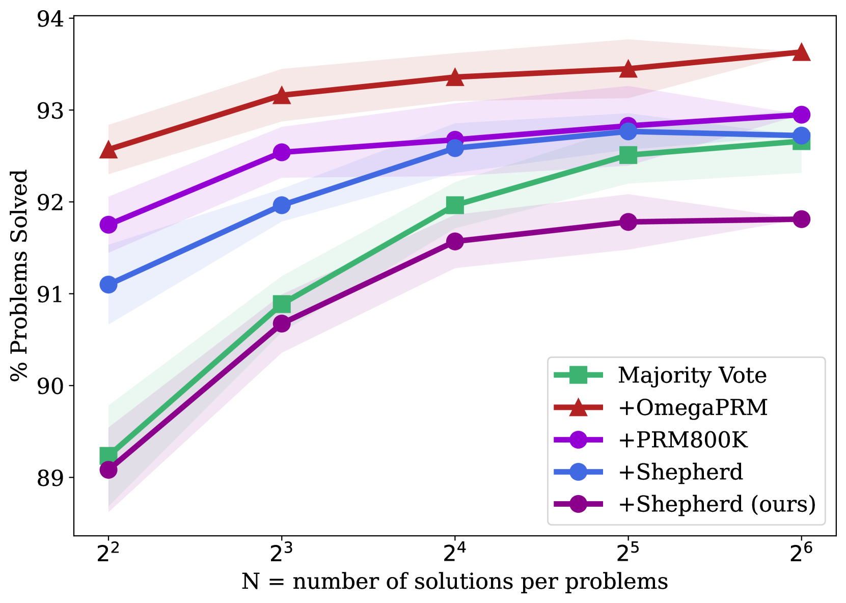
(b) Gemini Pro on GSM8K.
<details>
<summary>x6.png Details</summary>
### Visual Description
## Line Chart: Performance Scaling of Different Problem-Solving Methods
### Overview
This is a line chart comparing the performance of five different methods or models on a problem-solving task. The chart plots the percentage of problems solved against the number of solutions generated per problem (N), which is presented on a logarithmic scale (base 2). All methods show improved performance as N increases, with one method consistently outperforming the others.
### Components/Axes
* **X-Axis (Horizontal):** Labeled "N = number of solutions per problems". The axis uses a logarithmic scale with base 2, marked at points: 2² (4), 2³ (8), 2⁴ (16), 2⁵ (32), and 2⁶ (64).
* **Y-Axis (Vertical):** Labeled "% Problems Solved". The scale is linear, ranging from 40 to 60, with major tick marks at intervals of 5 (40, 45, 50, 55, 60).
* **Legend:** Located in the bottom-right quadrant of the chart area. It contains five entries, each with a unique color and marker symbol:
1. **Majority Vote:** Green line with square markers (■).
2. **+OmegaPRM:** Red line with upward-pointing triangle markers (▲).
3. **+PRM800K:** Purple line with circle markers (●).
4. **+Shepherd:** Blue line with circle markers (●).
5. **+Shepherd (ours):** Dark purple/magenta line with circle markers (●).
* **Data Series:** Each method is represented by a solid line connecting data points at each x-axis value. Each line is surrounded by a semi-transparent shaded band of the same color, likely representing a confidence interval or standard deviation.
### Detailed Analysis
**Trend Verification:** All five data series exhibit a clear upward, positive trend. As the number of solutions per problem (N) increases, the percentage of problems solved increases for every method. The rate of improvement appears to slow slightly at higher values of N (from 2⁵ to 2⁶).
**Data Point Extraction (Approximate Values):**
| Method (Legend Label) | Color/Marker | N=2² (4) | N=2³ (8) | N=2⁴ (16) | N=2⁵ (32) | N=2⁶ (64) |
| :--- | :--- | :--- | :--- | :--- | :--- | :--- |
| **+OmegaPRM** | Red / ▲ | ~47.5% | ~51.5% | ~54.8% | ~56.5% | ~58.2% |
| **+Shepherd** | Blue / ● | ~44.0% | ~49.5% | ~53.8% | ~56.0% | ~57.5% |
| **+PRM800K** | Purple / ● | ~46.0% | ~50.2% | ~53.2% | ~55.5% | ~57.2% |
| **Majority Vote** | Green / ■ | ~39.5% | ~46.0% | ~51.2% | ~54.2% | ~55.5% |
| **+Shepherd (ours)** | Dark Purple / ● | ~39.5% | ~45.8% | ~50.8% | ~53.2% | ~55.2% |
**Spatial Grounding & Cross-Reference:**
* The **+OmegaPRM** (red triangle) line is the highest at every data point.
* The **+Shepherd** (blue circle) and **+PRM800K** (purple circle) lines are closely clustered in the middle tier, with blue slightly above purple at most points.
* The **Majority Vote** (green square) and **+Shepherd (ours)** (dark purple circle) lines start at the lowest point (near 39.5% at N=4) and remain the two lowest-performing methods throughout, with green consistently slightly above dark purple.
### Key Observations
1. **Consistent Leader:** The **+OmegaPRM** method is the top performer across all tested values of N.
2. **Convergence at Scale:** The performance gap between the methods narrows as N increases. At N=4, the spread between the best and worst is ~8 percentage points. At N=64, the spread is ~3 percentage points.
3. **Method Grouping:** The methods naturally group into three tiers: Top (+OmegaPRM), Middle (+Shepherd, +PRM800K), and Bottom (Majority Vote, +Shepherd (ours)).
4. **Diminishing Returns:** The slope of all lines is steepest between N=4 and N=16, indicating the most significant gains in performance come from initial increases in the number of solutions. The curves begin to flatten between N=32 and N=64.
### Interpretation
This chart demonstrates the efficacy of different techniques for improving problem-solving accuracy through increased sampling (generating more solutions). The data suggests that:
* **Algorithmic Superiority:** The **+OmegaPRM** method provides a consistent and significant advantage over the other techniques, implying its underlying process for selecting or verifying solutions is more effective.
* **Value of Sampling:** All methods benefit from generating more solutions per problem, confirming that "brute-force" sampling combined with a selection mechanism is a viable strategy for boosting performance, though with diminishing returns.
* **Baseline Comparison:** The **Majority Vote** line serves as a baseline. The fact that **+Shepherd (ours)** performs similarly to, but slightly worse than, this baseline suggests that this particular implementation of the Shepherd method may not offer an advantage over simple majority voting for this specific task and metric. In contrast, the other **+Shepherd** (blue) method performs significantly better, indicating that implementation details or model versions are critical.
* **Practical Implication:** For resource-constrained applications, the chart helps identify a potential "sweet spot." For example, increasing N from 4 to 16 yields a large performance boost (~10-12% for most methods), while further increasing N to 64 yields a smaller additional gain (~3-4%). The optimal N would balance computational cost against the desired accuracy.
</details>
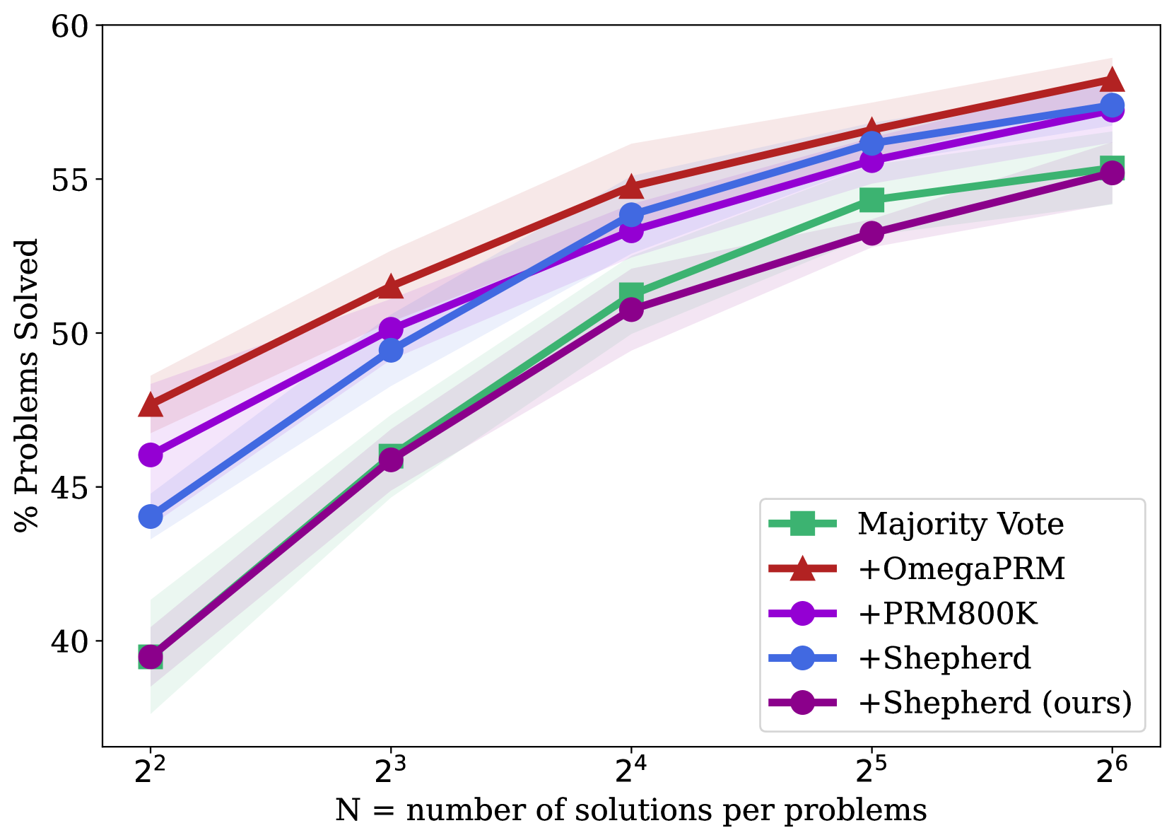
(c) Gemma2 27B on MATH500.
<details>
<summary>x7.png Details</summary>
### Visual Description
## Line Chart: Performance Scaling with Solution Count
### Overview
This line chart illustrates the performance scaling of five different methods for solving problems as the number of generated solutions per problem increases. The chart plots the percentage of problems solved against the number of solutions (N), which is presented on a logarithmic scale (base 2). All methods show improved performance with more solutions, but they start at different baselines and converge at higher N.
### Components/Axes
* **Chart Type:** Line chart with shaded confidence intervals or variance bands.
* **X-Axis:**
* **Label:** `N = number of solutions per problems`
* **Scale:** Logarithmic (base 2).
* **Ticks/Markers:** `2²` (4), `2³` (8), `2⁴` (16), `2⁵` (32), `2⁶` (64).
* **Y-Axis:**
* **Label:** `% Problems Solved`
* **Scale:** Linear, ranging from approximately 72% to 93%.
* **Ticks/Markers:** 75, 80, 85, 90.
* **Legend (Located in the bottom-right quadrant):**
* **Green Square Line:** `Majority Vote`
* **Red Triangle Line:** `+OmegaPRM`
* **Purple Circle Line:** `+PRM800K`
* **Blue Circle Line:** `+Shepherd`
* **Dark Purple Circle Line:** `+Shepherd (ours)`
### Detailed Analysis
**Data Series and Approximate Values:**
1. **Majority Vote (Green, Square markers):**
* **Trend:** Starts lowest, shows the steepest initial improvement, and continues to climb steadily.
* **Data Points:**
* N=4: ~72.5%
* N=8: ~82%
* N=16: ~87%
* N=32: ~89.5%
* N=64: ~90.5%
2. **+OmegaPRM (Red, Triangle markers):**
* **Trend:** Starts as the highest-performing method and maintains a lead throughout, with a steady, slightly flattening increase.
* **Data Points:**
* N=4: ~86.5%
* N=8: ~90%
* N=16: ~91.5%
* N=32: ~92.5%
* N=64: ~93%
3. **+PRM800K (Purple, Circle markers):**
* **Trend:** Starts as the second-highest, follows a similar trajectory to +OmegaPRM but remains slightly below it.
* **Data Points:**
* N=4: ~85%
* N=8: ~89%
* N=16: ~90.5%
* N=32: ~91.5%
* N=64: ~92%
4. **+Shepherd (Blue, Circle markers):**
* **Trend:** Starts in the middle of the pack, shows strong improvement, and nearly catches up to the top methods at N=64.
* **Data Points:**
* N=4: ~74%
* N=8: ~83%
* N=16: ~88%
* N=32: ~89.5%
* N=64: ~91%
5. **+Shepherd (ours) (Dark Purple, Circle markers):**
* **Trend:** Starts just below +PRM800K and follows a nearly identical, parallel trajectory, ending very close to it.
* **Data Points:**
* N=4: ~83.5%
* N=8: ~88%
* N=16: ~90.5%
* N=32: ~91%
* N=64: ~91.5%
### Key Observations
1. **Performance Hierarchy:** At low solution counts (N=4), there is a clear performance hierarchy: `+OmegaPRM` > `+PRM800K` > `+Shepherd (ours)` > `+Shepherd` > `Majority Vote`.
2. **Convergence:** As N increases to 64, the performance gap between all methods narrows significantly. The top four methods (`+OmegaPRM`, `+PRM800K`, `+Shepherd`, `+Shepherd (ours)`) converge within a ~2% range (91%-93%).
3. **Scaling Efficiency:** `Majority Vote` and `+Shepherd` show the most dramatic relative improvement from N=4 to N=64, indicating they benefit most from increased solution diversity. The top methods (`+OmegaPRM`, `+PRM800K`) show more modest, incremental gains, suggesting they are more efficient with fewer solutions.
4. **Method Grouping:** The chart visually groups the methods into two clusters: the top-performing trio (`+OmegaPRM`, `+PRM800K`, `+Shepherd (ours)`) and the lower-starting pair (`+Shepherd`, `Majority Vote`), though the latter pair closes the gap considerably.
### Interpretation
This chart demonstrates the principle of **scaling test-time compute** in problem-solving AI systems. The key insight is that generating and evaluating multiple candidate solutions (increasing N) reliably improves performance for all tested methods.
* **What the data suggests:** The methods prefixed with "+" (likely representing some form of process reward model or verifier) consistently outperform the baseline `Majority Vote` approach, especially when solution counts are low. This indicates that using a learned verifier to score or select solutions is more effective than simple consensus.
* **Relationship between elements:** The x-axis (N) is the independent variable representing resource投入 (compute). The y-axis (% Solved) is the dependent outcome. The different lines represent different algorithms for utilizing that compute. The shaded bands suggest variability in performance, likely across multiple runs or problem subsets.
* **Notable trends/anomalies:** The most significant trend is the **diminishing returns** for the top methods. Moving from N=32 to N=64 yields a smaller gain than moving from N=4 to N=8. This implies an efficiency ceiling. The near-parallel trajectories of `+PRM800K` and `+Shepherd (ours)` suggest these two methods may be fundamentally similar in their scaling behavior, despite potential differences in training data or architecture. The chart argues that while advanced verifiers (`+OmegaPRM`) provide a better starting point, the advantage they confer becomes less critical as you are willing to spend more compute (higher N) on generating solutions.
</details>
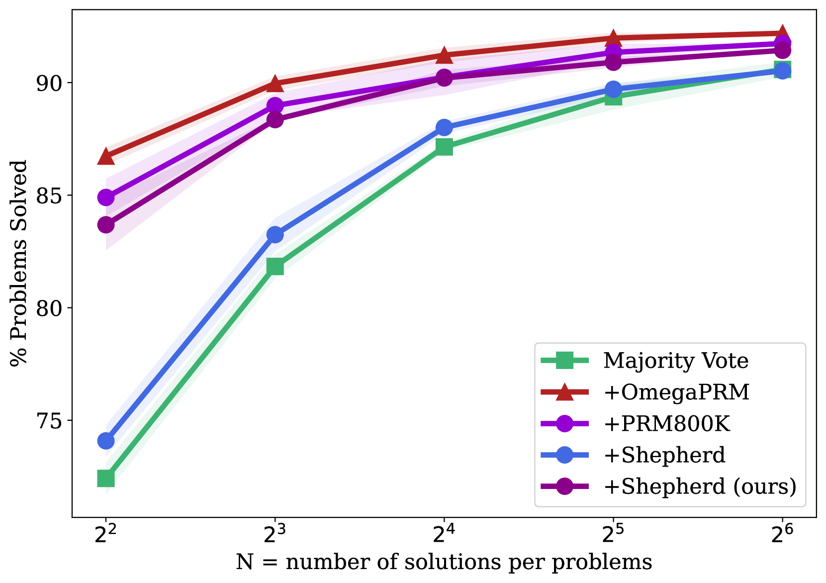
(d) Gemma2 27B on GSM8K.
Figure 3: A comparison of PRMs trained with different process supervision datasets, evaluated by their ability to search over many test solutions using a PRM-weighted majority voting. We visualize the variance across many sub-samples of the $128$ solutions we generated in total per problem.
Table 1: The performance comparison of PRMs trained with different process supervision datasets. The numbers represent the percentage of problems solved using PRM-weighted majority voting with $k=64$ .
| MajorityVote@64 + Math-Shepherd + Math-Shepherd (our impl) | 67.2 67.2 67.2 | 54.7 57.4 55.2 | 92.7 92.7 91.8 | 90.6 90.5 91.4 |
| --- | --- | --- | --- | --- |
| + PRM800K | 67.6 | 57.2 | 92.9 | 91.7 |
| + OmegaPRM | 69.4 | 58.2 | 93.6 | 92.2 |
Table 1 and Fig. 3 presents the performance comparison of PRMs trained on various process annotation datasets. OmegaPRM consistently outperforms the other process supervision datasets. Specifically, the fine-tuned Gemini Pro achieves $69.4$ % and $93.6$ % accuracy on MATH500 and GSM8K, respectively, using OmegaPRM-weighted majority voting. For the pretrained Gemma2 27B, it also performs the best with $58.2$ % and $92.2$ % accuracy on MATH500 and GSM8K, respectively. It shows superior performance comparing to both human annotated PRM800K but also automatic annotated Math-Shepherd. More specifically, when the number of samples is small, almost all the PRM models outperforme the majority vote. However, as the number of samples increases, the performance of other PRMs gradually converges to the same level of the majority vote. In contrast, our PRM model continues to demonstrate a clear margin of accuracy.
### 4.2 Step Distribution
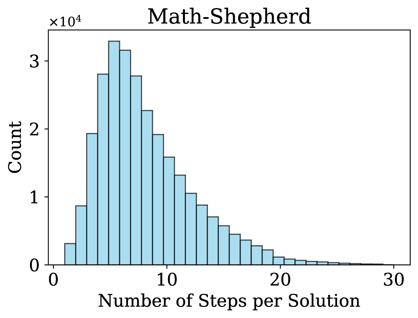
An important factor in process supervision is the number of steps in a solution and the length of each step. Previous works (Lightman et al., 2023; Wang et al., 2024a, b) use rule-based strategies to split a solution into steps, e.g., using newline as delimiters. In contrast, we propose a more flexible method for step division, treating any sequence of consecutive tokens in a solution as a valid step. We observe that many step divisions in Math-Shepherd lack semantic coherence to some extent. Therefore, we hypothesize that semantically explicit cutting is not necessary for training a PRM.
<details>
<summary>x8.png Details</summary>
### Visual Description
## Histogram: Math-Shepherd Step Distribution
### Overview
The image is a histogram titled "Math-Shepherd" that displays the frequency distribution of the number of steps required to solve problems within a dataset or system called "Math-Shepherd." The chart shows a right-skewed distribution, indicating that most solutions require a relatively small number of steps, with a long tail of solutions requiring many more steps.
### Components/Axes
* **Title:** "Math-Shepherd" (centered at the top).
* **X-Axis:**
* **Label:** "Number of Steps per Solution" (centered below the axis).
* **Scale:** Linear scale from 0 to 30, with major tick marks at 0, 10, 20, and 30.
* **Y-Axis:**
* **Label:** "Count" (rotated vertically on the left side).
* **Scale:** Linear scale from 0 to 3, with a multiplier of **×10⁴** (10,000) indicated at the top-left corner of the axis. Major tick marks are at 0, 1, 2, and 3 (representing 0, 10,000, 20,000, and 30,000 respectively).
* **Data Series:** A single series represented by light blue bars with black outlines. There is no legend, as there is only one data category.
### Detailed Analysis
The histogram consists of approximately 30 bars, each representing a bin for the number of steps (likely 1-step bins from 1 to 30). The height of each bar corresponds to the count of solutions falling within that step range.
**Trend Verification:** The visual trend shows a rapid increase in count from 1 step to a peak, followed by a steady, gradual decline as the number of steps increases. The distribution is positively skewed (right-skewed).
**Estimated Data Points (Approximate Values):**
* **Peak:** The highest bar is located at approximately **6 steps**. Its height is slightly above the 3 mark on the y-axis, indicating a count of **~32,000** (3.2 × 10⁴).
* **Adjacent Peaks:** The bars for 5 and 7 steps are also very high, at approximately **~28,000** and **~31,000** respectively.
* **Rise:** The count increases sharply from ~3,000 at 1 step to the peak at 6 steps.
* **Decline:** After the peak, the count decreases steadily. By 10 steps, the count is approximately **~19,000**. By 15 steps, it is approximately **~7,000**. By 20 steps, it is approximately **~2,000**. The tail extends to 30 steps, where the count is very low, likely in the low hundreds or less.
### Key Observations
1. **Dominant Mode:** The vast majority of solutions in the Math-Shepherd dataset are completed in **fewer than 15 steps**, with the highest concentration between 4 and 10 steps.
2. **Right Skew:** The distribution has a long right tail, indicating the presence of a smaller number of problems that are significantly more complex, requiring 20, 25, or even 30 steps to solve.
3. **Unimodal Distribution:** There is a single, clear peak, suggesting a central tendency around 5-7 steps for problem complexity.
4. **Scale:** The total number of solutions represented is large. A rough visual integration suggests the total count is likely in the range of **200,000 to 300,000** solutions.
### Interpretation
This histogram characterizes the computational or logical complexity of the Math-Shepherd dataset. The data suggests that:
* **Core Complexity:** The "typical" or most common problem in this set can be solved in a moderate number of steps (5-7). This defines the baseline complexity for the system.
* **Problem Spectrum:** The dataset contains a full spectrum of difficulty, from very simple (1-3 steps) to highly complex (25+ steps). The right skew is typical for many real-world problem sets, where most tasks are of moderate difficulty, and extreme outliers are rare.
* **System Implications:** For an AI or algorithm being tested on Math-Shepherd, performance on the 4-10 step range is critical, as this represents the bulk of the data. However, robustness would be measured by its ability to handle the long tail of complex problems. The distribution provides a benchmark for expected solution length and can be used to analyze the efficiency of different solving methods.
</details>
<details>
<summary>x9.png Details</summary>
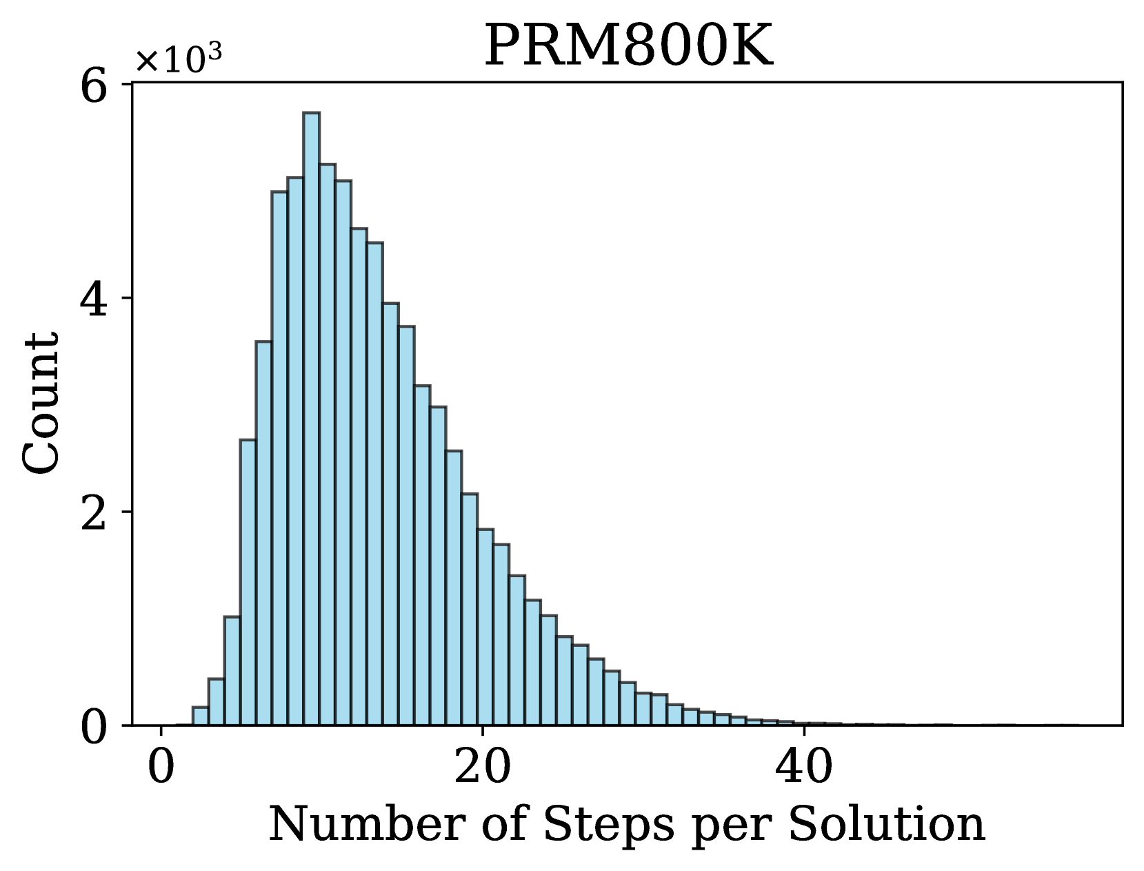
### Visual Description
## Histogram: PRM800K Step Distribution
### Overview
The image displays a histogram titled "PRM800K," illustrating the frequency distribution of the number of steps required for solutions within a dataset or process named PRM800K. The chart shows a right-skewed distribution, indicating that most solutions require a relatively low number of steps, with a long tail of less frequent, more complex solutions.
### Components/Axes
* **Title:** "PRM800K" (centered at the top of the chart).
* **X-Axis:**
* **Label:** "Number of Steps per Solution" (centered below the axis).
* **Scale:** Linear scale from 0 to approximately 45.
* **Major Tick Marks:** Labeled at 0, 20, and 40.
* **Y-Axis:**
* **Label:** "Count" (rotated 90 degrees, positioned to the left of the axis).
* **Scale:** Linear scale from 0 to 6, with a multiplier of "×10³" (indicating thousands) positioned at the top-left of the axis.
* **Major Tick Marks:** Labeled at 0, 2, 4, and 6 (representing 0, 2000, 4000, and 6000 counts).
* **Data Series:** A single series represented by vertical bars (bins). The bars are filled with a light blue color and have thin black outlines.
### Detailed Analysis
* **Distribution Shape:** The histogram is unimodal and right-skewed (positively skewed). The tail extends much further to the right (higher step counts) than to the left.
* **Peak (Mode):** The highest frequency occurs in the bin corresponding to approximately **10-12 steps per solution**. The peak bar reaches a count of approximately **5,800** (just below the 6 ×10³ mark).
* **Range:** The visible data spans from approximately **2 steps** (the first non-zero bar) to about **42 steps**. The frequency becomes negligible (near zero) beyond 40 steps.
* **Key Frequency Points (Approximate):**
* **~5 steps:** Count ≈ 1,000
* **~10 steps (Peak):** Count ≈ 5,800
* **~15 steps:** Count ≈ 4,000
* **~20 steps:** Count ≈ 2,200
* **~25 steps:** Count ≈ 1,000
* **~30 steps:** Count ≈ 400
* **~35 steps:** Count ≈ 100
* **~40 steps:** Count ≈ 20 (very low)
### Key Observations
1. **Concentration of Data:** The vast majority of solutions are completed in **fewer than 20 steps**. The area under the curve from 0 to 20 steps contains the overwhelming majority of the total count.
2. **Rapid Decline:** After the peak at ~10-12 steps, the frequency declines steadily and significantly. The drop from the peak to 20 steps is steep.
3. **Long Tail:** A persistent, low-frequency tail extends to the right, indicating that while rare, solutions requiring 30, 35, or even 40+ steps do exist in the PRM800K dataset.
4. **Absence of Very Short Solutions:** There appear to be no solutions with 0 or 1 step, as the first visible bar starts around 2 steps.
### Interpretation
This histogram characterizes the computational or procedural complexity of the PRM800K dataset. The right-skewed distribution is typical for many real-world processes where simple tasks are common and complex tasks are rare.
* **What it Suggests:** The data implies that the problem space or algorithm generating these solutions is generally efficient, with most instances solvable through a moderate number of steps (centered around a dozen). The long tail suggests the presence of "hard" or "outlier" problems that require significantly more effort.
* **Relationship Between Elements:** The x-axis (step count) is the independent variable measuring complexity, while the y-axis (count) shows how commonly each complexity level occurs. The shape of the distribution directly answers the question: "How many steps does a typical solution in PRM800K require?"
* **Notable Anomalies/Trends:** The most notable trend is the smooth, unimodal decay after the peak. There are no secondary peaks or gaps, suggesting a continuous spectrum of problem difficulty rather than distinct clusters of "easy," "medium," and "hard" problems. The absence of 0-1 step solutions might indicate a minimum baseline complexity for any valid solution in this dataset.
</details>
Figure 4: Number of steps distribution.
In practice, we first examine the distribution of the number of steps per solution in PRM800K and Math-Shepherd, as shown in Fig. 4, noting that most solutions have less than $20$ steps. During binary search, we aim to divide a full solution into $16$ pieces. To calculate the expected step length, we divide the average solution length by $16$ . The binary search terminates when a step is shorter than this value. The resulting distributions of step lengths for OmegaPRM and the other two datasets are shown in Fig. 5. This flexible splitting strategy produces a step length distribution similar to that of the rule-based strategy.
<details>
<summary>x10.png Details</summary>
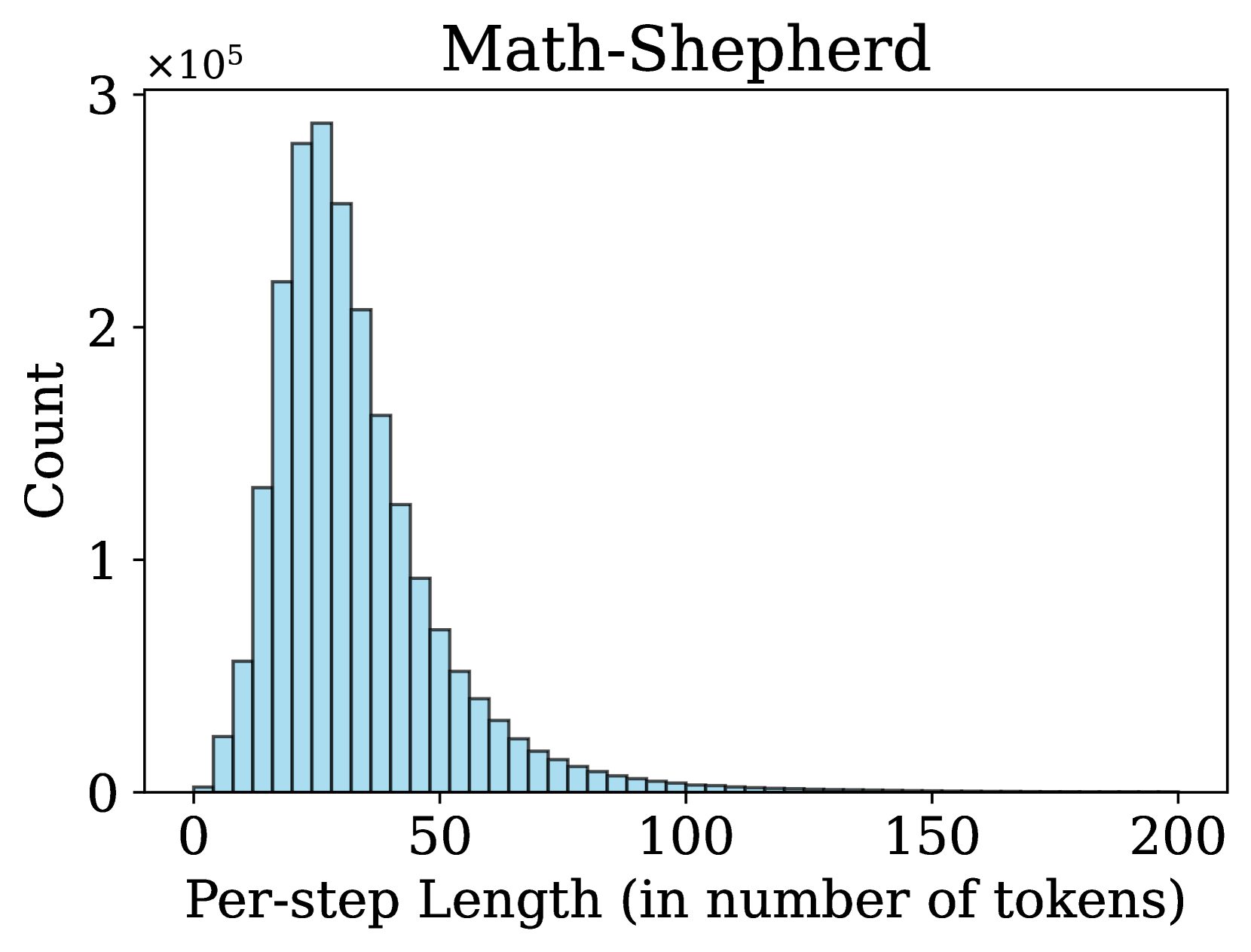
### Visual Description
## Histogram: Math-Shepherd Per-step Token Length Distribution
### Overview
The image displays a histogram titled "Math-Shepherd," illustrating the frequency distribution of per-step lengths, measured in the number of tokens. The data is presented as a series of vertical bars (bins) on a 2D plot, showing a right-skewed distribution.
### Components/Axes
* **Title:** "Math-Shepherd" (centered at the top).
* **Y-axis:**
* **Label:** "Count" (rotated vertically on the left side).
* **Scale:** Linear scale from 0 to 3, with a multiplier of `×10⁵` indicated at the top-left corner of the axis. This means the values represent hundreds of thousands (e.g., 1 = 100,000).
* **Major Ticks:** 0, 1, 2, 3.
* **X-axis:**
* **Label:** "Per-step Length (in number of tokens)" (centered at the bottom).
* **Scale:** Linear scale from 0 to 200.
* **Major Ticks:** 0, 50, 100, 150, 200.
* **Data Series:** A single data series represented by light blue vertical bars. Each bar's height corresponds to the count of steps falling within a specific token-length bin. The bin width appears to be approximately 5 tokens.
### Detailed Analysis
* **Distribution Shape:** The histogram is strongly right-skewed (positively skewed). The tail extends far to the right, indicating a long tail of less frequent, longer steps.
* **Peak (Mode):** The highest frequency occurs in the bin centered approximately between 20 and 30 tokens. The peak count is just below the 3 mark on the y-axis, representing an estimated **~290,000 occurrences** (with uncertainty due to visual estimation).
* **Trend Verification:**
* **Left Slope (0 to ~25 tokens):** The line of bar tops slopes steeply upward from near zero at 0 tokens to the peak.
* **Right Slope (~25 to 200 tokens):** The line of bar tops slopes downward, initially steeply until about 50 tokens, then more gradually, approaching zero count as the per-step length nears 200 tokens.
* **Key Data Points (Approximate):**
* **~10 tokens:** Count ≈ 50,000
* **~20 tokens:** Count ≈ 220,000
* **~25 tokens (Peak):** Count ≈ 290,000
* **~30 tokens:** Count ≈ 250,000
* **~50 tokens:** Count ≈ 90,000
* **~100 tokens:** Count is very low, visually estimated at < 5,000.
* **>150 tokens:** Counts are negligible, approaching zero.
### Key Observations
1. **Concentration of Short Steps:** The vast majority of steps in the "Math-Shepherd" dataset are short, with the highest concentration between approximately 15 and 40 tokens.
2. **Long Tail:** While most steps are short, there is a persistent, long tail of steps extending to 200 tokens and likely beyond, though their frequency is extremely low.
3. **Unimodal Distribution:** The data has a single, clear peak, suggesting a common or typical step length around 25 tokens.
4. **Rapid Drop-off:** The frequency drops off very sharply after the peak, indicating that steps significantly longer than the mode are considerably less common.
### Interpretation
This histogram characterizes the token-length profile of steps within a dataset or process named "Math-Shepherd," which is likely related to mathematical reasoning or problem-solving given the name.
* **What the data suggests:** The distribution implies that the "Math-Shepherd" process or dataset is composed predominantly of short, concise steps (averaging around 25 tokens). This could reflect a dataset of brief reasoning steps, intermediate calculations, or sub-problems in mathematical proofs. The long tail indicates that while rare, some steps require significantly more verbose explanations or computations.
* **How elements relate:** The x-axis (token length) is the independent variable being measured, and the y-axis (count) shows how frequently each length occurs. The shape of the histogram directly visualizes the underlying probability distribution of step lengths.
* **Notable anomalies/trends:** The most notable feature is the extreme right skew. This is not a normal (Gaussian) distribution. It suggests a generative process where short outputs are highly probable, and the probability of generating a step decreases rapidly as the required length increases. This pattern is common in natural language and code generation tasks. The absence of any significant secondary peaks indicates a consistent, unimodal process for generating these steps.
</details>
<details>
<summary>x11.png Details</summary>
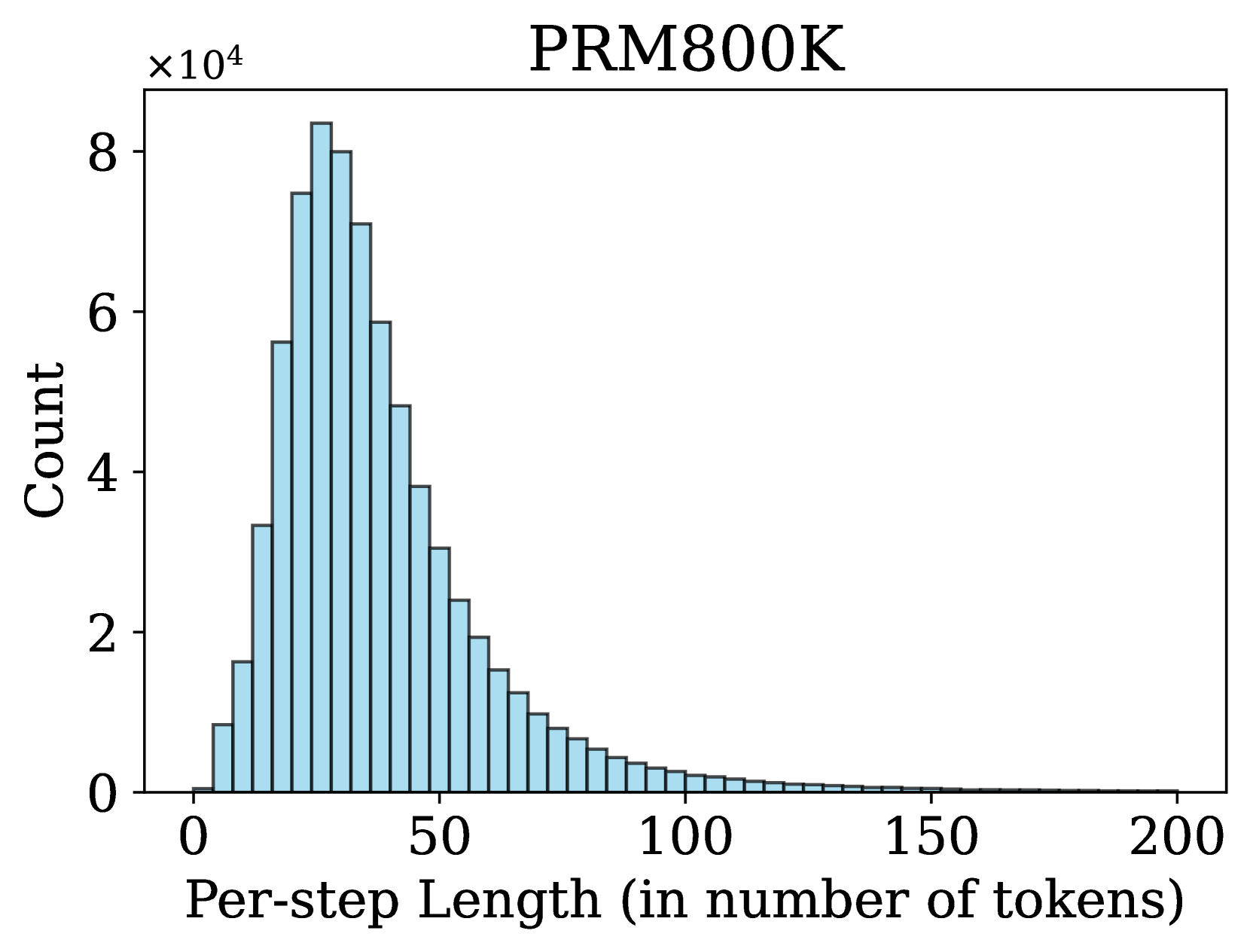
### Visual Description
## Histogram: PRM800K Per-step Length Distribution
### Overview
The image displays a histogram titled "PRM800K" that visualizes the frequency distribution of per-step lengths, measured in the number of tokens. The chart shows a right-skewed distribution, indicating that most steps are relatively short, with a long tail of less frequent, longer steps.
### Components/Axes
* **Title:** "PRM800K" (centered at the top).
* **Y-axis:**
* **Label:** "Count" (rotated vertically on the left).
* **Scale:** Linear scale with a multiplier of `×10⁴` (indicated at the top-left of the axis).
* **Tick Marks:** Major ticks are labeled at 0, 2, 4, 6, and 8. These correspond to counts of 0, 20,000, 40,000, 60,000, and 80,000, respectively.
* **X-axis:**
* **Label:** "Per-step Length (in number of tokens)" (centered at the bottom).
* **Scale:** Linear scale.
* **Tick Marks:** Major ticks are labeled at 0, 50, 100, 150, and 200.
* **Data Series:** A single series represented by light blue vertical bars. Each bar's height represents the count of steps falling within a specific token-length bin.
### Detailed Analysis
* **Distribution Shape:** The histogram is unimodal and strongly right-skewed (positively skewed). The tail extends far to the right.
* **Peak (Mode):** The highest frequency occurs in the bin centered approximately at **25 tokens**. The bar height at this peak is approximately **8.2 × 10⁴ (82,000)**.
* **Range:** The visible data spans from near 0 tokens to just beyond 200 tokens. The vast majority of the data is concentrated below 100 tokens.
* **Key Frequency Estimates (Approximate):**
* **~10 tokens:** ~1.8 × 10⁴ (18,000)
* **~20 tokens:** ~7.5 × 10⁴ (75,000)
* **~25 tokens (Peak):** ~8.2 × 10⁴ (82,000)
* **~30 tokens:** ~8.0 × 10⁴ (80,000)
* **~50 tokens:** ~3.0 × 10⁴ (30,000)
* **~75 tokens:** ~1.0 × 10⁴ (10,000)
* **~100 tokens:** ~0.3 × 10⁴ (3,000)
* **Beyond 150 tokens:** The counts become very low, approaching zero on this scale.
### Key Observations
1. **Concentration of Short Steps:** The overwhelming majority of per-step lengths are short, with the bulk of the distribution lying between approximately 10 and 60 tokens.
2. **Sharp Rise and Gradual Decline:** The frequency rises sharply from 0 to the peak at ~25 tokens and then declines more gradually, creating the characteristic right skew.
3. **Long Tail:** There is a persistent, low-frequency tail extending to 200 tokens and likely beyond, indicating the presence of rare but significantly longer steps.
4. **Mode vs. Median/Mean:** Due to the right skew, the mode (~25 tokens) is less than the median, which in turn is less than the mean. The average step length is pulled higher by the long tail.
### Interpretation
This histogram characterizes the step-length profile of the "PRM800K" dataset or process. The data suggests a system where the typical operational unit (a "step") is concise, often involving around 20-30 tokens. This could reflect, for example, the length of reasoning steps in a process reward model (PRM), short dialogue turns, or brief procedural instructions.
The right-skewed distribution is common in natural language and behavioral data. It implies that while efficiency or brevity is the norm (the high peak), the system must also accommodate occasional, substantially more complex or verbose steps (the long tail). The sparsity of data beyond 100 tokens indicates that such long steps are exceptional events. For technical planning, this distribution informs requirements for context window allocation, memory usage, and performance optimization, highlighting that resources must be sized to handle the common short cases efficiently while not failing on the rare long ones.
</details>
<details>
<summary>x12.png Details</summary>
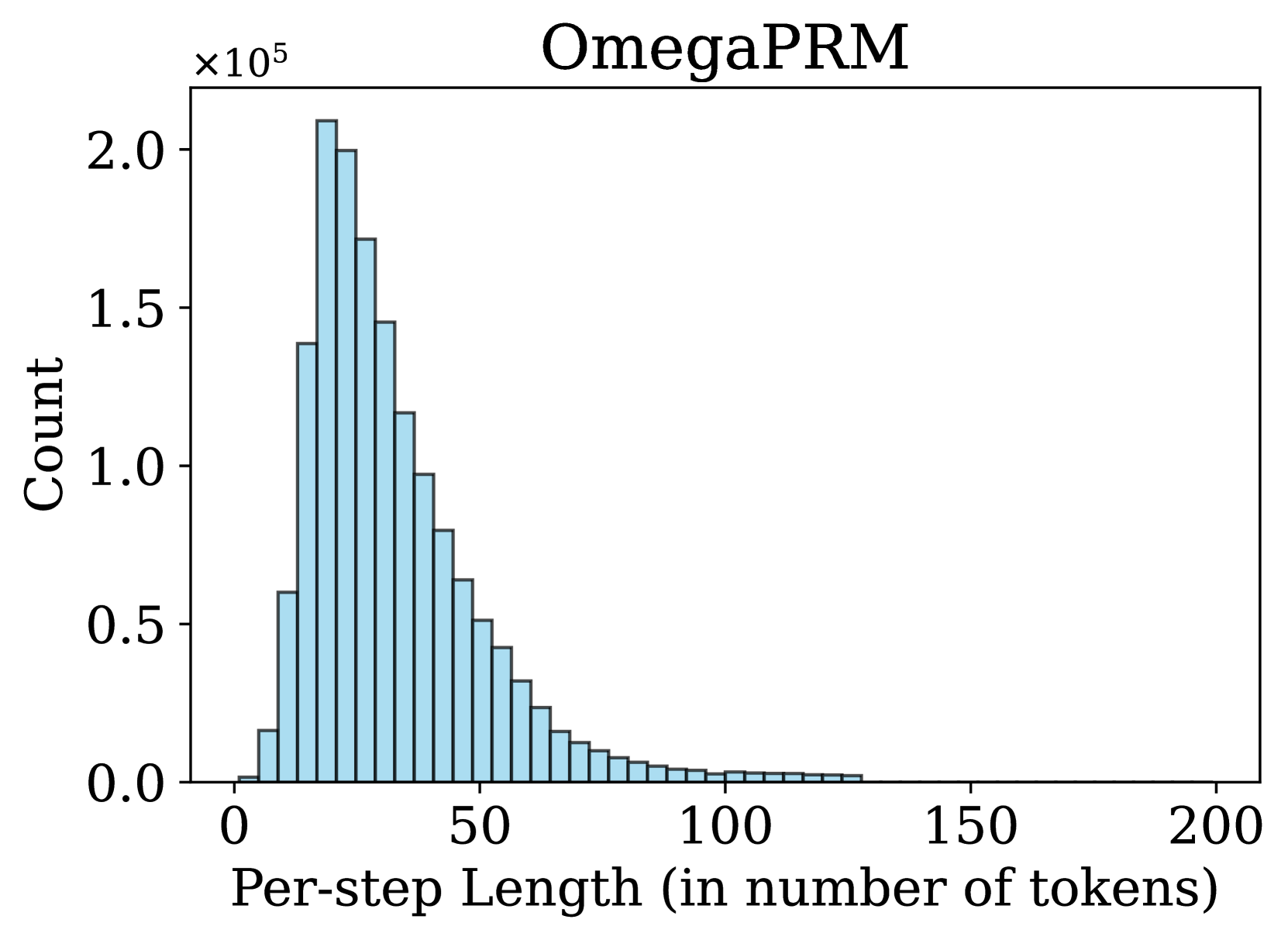
### Visual Description
## Histogram: OmegaPRM Per-step Token Length Distribution
### Overview
The image is a histogram titled "OmegaPRM" that visualizes the frequency distribution of per-step lengths, measured in the number of tokens. The chart displays a single data series represented by light blue bars, showing how many times (count) steps of various token lengths occur within the OmegaPRM dataset or process.
### Components/Axes
* **Title:** "OmegaPRM" (Top center).
* **Y-axis:** Labeled "Count". The scale is linear and includes a multiplier notation "×10⁵" at the top-left of the axis. Major tick marks are at 0.0, 0.5, 1.0, 1.5, and 2.0, representing counts from 0 to 200,000.
* **X-axis:** Labeled "Per-step Length (in number of tokens)". The scale is linear with major tick marks at 0, 50, 100, 150, and 200.
* **Data Series:** A single series of adjacent, light blue bars with black outlines. There is no legend, as only one category is plotted.
### Detailed Analysis
The histogram shows a **right-skewed (positively skewed) distribution**. The trend is a sharp rise to a peak followed by a long, gradual tail extending to the right.
* **Peak (Mode):** The highest frequency occurs for per-step lengths in the approximate range of **20-25 tokens**. The bar at this peak reaches a count of approximately **2.1 x 10⁵ (210,000)**.
* **Distribution Shape:**
* The count rises steeply from near zero at 0 tokens to the peak.
* After the peak, the count decreases steadily. By a length of 50 tokens, the count has fallen to roughly **0.6 x 10⁵ (60,000)**.
* The decline continues, becoming more gradual. At 100 tokens, the count is very low, approximately **0.05 x 10⁵ (5,000)** or less.
* The visible data tail ends around **125-130 tokens**, with counts approaching zero. The x-axis extends to 200, but no significant data is present beyond ~130.
* **Range:** The vast majority of per-step lengths fall between **~5 and ~100 tokens**. Steps shorter than 5 tokens or longer than 100 tokens are comparatively rare.
### Key Observations
1. **Strong Right Skew:** The distribution is not symmetric. The mean per-step length is likely greater than the median, which is greater than the mode (~22 tokens), due to the long tail of longer steps.
2. **Concentrated Mass:** The highest density of data is concentrated in a relatively narrow band between approximately 10 and 40 tokens.
3. **Absence of Very Long Steps:** There is no visible data for steps approaching 200 tokens, suggesting an upper bound or extreme rarity for steps of that length in this dataset.
### Interpretation
This histogram characterizes the "Per-step Length" for a system or dataset named "OmegaPRM." The data suggests that the process generating these steps most commonly produces outputs of moderate length (around 20-25 tokens). The right-skewed nature indicates that while short-to-moderate steps are the norm, there is a significant, diminishing probability of encountering progressively longer steps.
In a technical context, this could represent:
* The length of individual reasoning steps in a chain-of-thought process.
* The size of data chunks processed in an iterative algorithm.
* The length of generated text segments in a language model task.
The distribution implies that the system is optimized for or naturally tends toward concise steps, but retains the capacity for longer, more complex steps when necessary, albeit with decreasing frequency. The lack of steps near 200 tokens may indicate a practical or imposed limit on step length.
</details>
Figure 5: Step length distribution in terms of number of tokens.
### 4.3 PRM Training Objectives
Table 2: Comparison of different training objectives for PRMs.
| PRM Accuracy (%) | Soft Label 70.1 | Hard Label 63.3 | Pairwise 64.2 |
| --- | --- | --- | --- |
As outlined in Section 3.4, PRMs can be trained using multiple objectives. We construct a small process supervision test set using the problems from the MATH test split. We train PRMs using pointwise soft label, pointwise hard label and pairwise loss respectively, and evaluate how accurately they can classify the per-step correctness. Table 2 presents the comparison of different objectives, and the pointwise soft label is the best among them with $70.1$ % accuracy.
### 4.4 Algorithm Efficiency
As described in Section Section 3.2 and Section 3.3, we utilize binary search and Monte Carlo Tree Search to improve the efficiency of OmegaPRM process supervision data collection by effectively identifying the first incorrect step and reusing rollouts in Monte Carlo estimation. To quantitatively measure the efficiency of OmegaPRM, we collected process supervision data using both brute-force-style method (Wang et al., 2024a, b) and OmegaPRM with the same computational budget. As a result, we were able to generate $200$ K data points using the brute-force algorithm compared to $15$ million data points with OmegaPRM, demonstrating a $75$ -times efficiency improvement. In practice, we randomly down-sampled OmegaPRM data to $1.5$ million for PRM training.
## 5 Limitations
There are some limitations with our paper, which we reserve for future work:
#### Automatic process annotation is noisy.
Our method for automatic process supervision annotation introduces noise in the form of false positives and negatives, but experiments indicate that it can still effectively train a PRM. The PRM trained on our dataset performs better than one trained on the human-annotated PRM800K dataset. The precise impact of noise on PRM performance remains uncertain. For future research, a comprehensive comparison of human and automated annotations should be conducted. One other idea is to integrate human and automated annotations, which could result in more robust and efficient process supervision.
#### Human supervision is still necessary.
Unlike the work presented in AlphaGo Zero (Silver et al., 2017), our method requires the question and golden answer pair. The question is necessary for LLM to start the MCTS and the golden answer is inevitable for the LLM to compare its rollouts with and determine the correctness of the current step. This will limit the method to the tasks with such question and golden answer pairs. Therefore, we need to adapt the current method further to make it suitable for open-ended tasks.
## 6 Conclusion
In conclusion, we introduce OmegaPRM, a divide-and-conquer Monte Carlo Tree Search algorithm, designed to automate the process supervision data collection for LLMs. By efficiently pinpointing the first error in the Chain-of-Thought and balancing data quality, OmegaPRM addresses the shortcomings of existing methods. Our automated approach enables the collection of over 1.5 million process supervision annotations, which are used to train a PRM. Leveraging this automated process supervision with the weighted self-consistency algorithm, we improve LLM mathematical reasoning performance, achieving a 69.4% success rate on the MATH benchmark — a 18.4% absolute increase over the base model which amounts to a relative improvement of 36%. Additionally, our method significantly reduces data collection costs compared to human annotation and brute force Monte-Carlo sampling. These findings highlight OmegaPRM’s potential to enhance LLM capabilities in complex multi-step reasoning tasks.
## 7 Acknowledgements
We would like to express our deepest gratitude to Matt Barnes, Jindong Chen and Rif A. Saurous, for their support and helpful feedback to our work. We also thank Peiyi Wang for clarifying the details in Math-Shepherd and providing insightful suggestions.
## References
- Christiano et al. (2017) P. Christiano, J. Leike, T. B. Brown, M. Martic, S. Legg, and D. Amodei. Deep reinforcement learning from human preferences. arXiv preprint arXiv:1706.03741, 2017.
- Cobbe et al. (2021) K. Cobbe, V. Kosaraju, M. Bavarian, M. Chen, H. Jun, L. Kaiser, M. Plappert, J. Tworek, J. Hilton, R. Nakano, C. Hesse, and J. Schulman. Training verifiers to solve math word problems. arXiv preprint arXiv:2110.14168, 2021.
- Feng et al. (2023) X. Feng, Z. Wan, M. Wen, S. M. McAleer, Y. Wen, W. Zhang, and J. Wang. Alphazero-like tree-search can guide large language model decoding and training. arXiv preprint arXiv:2309.17179, 2023.
- Feng et al. (2024) X. Feng, Z. Wan, M. Wen, S. M. McAleer, Y. Wen, W. Zhang, and J. Wang. Alphazero-like tree-search can guide large language model decoding and training. arXiv preprint arXiv:2309.17179, 2024.
- Fu et al. (2023) Y. Fu, H. Peng, A. Sabharwal, P. Clark, and T. Khot. Complexity-based prompting for multi-step reasoning. In Proceedings of the 11th International Conference on Learning Representations (ICLR), May 2023.
- Gemini Team et al. (2024) Gemini Team, M. Reid, N. Savinov, D. Teplyashin, Dmitry, Lepikhin, T. Lillicrap, J. baptiste Alayrac, R. Soricut, A. Lazaridou, O. Firat, J. Schrittwieser, I. Antonoglou, R. Anil, S. Borgeaud, A. Dai, K. Millican, E. Dyer, M. Glaese, T. Sottiaux, B. Lee, F. Viola, M. Reynolds, Y. Xu, J. Molloy, J. Chen, M. Isard, P. Barham, T. Hennigan, R. McIlroy, M. Johnson, J. Schalkwyk, E. Collins, E. Rutherford, E. Moreira, K. Ayoub, M. Goel, C. Meyer, G. Thornton, Z. Yang, H. Michalewski, Z. Abbas, N. Schucher, A. Anand, R. Ives, J. Keeling, K. Lenc, S. Haykal, S. Shakeri, P. Shyam, A. Chowdhery, R. Ring, S. Spencer, E. Sezener, L. Vilnis, O. Chang, N. Morioka, G. Tucker, C. Zheng, O. Woodman, N. Attaluri, T. Kocisky, E. Eltyshev, X. Chen, T. Chung, V. Selo, S. Brahma, P. Georgiev, A. Slone, Z. Zhu, J. Lottes, S. Qiao, B. Caine, S. Riedel, A. Tomala, M. Chadwick, J. Love, P. Choy, S. Mittal, N. Houlsby, Y. Tang, M. Lamm, L. Bai, Q. Zhang, L. He, Y. Cheng, P. Humphreys, Y. Li, S. Brin, A. Cassirer, Y. Miao, L. Zilka, T. Tobin, K. Xu, L. Proleev, D. Sohn, A. Magni, L. A. Hendricks, I. Gao, S. Ontanon, O. Bunyan, N. Byrd, A. Sharma, B. Zhang, M. Pinto, R. Sinha, H. Mehta, D. Jia, S. Caelles, A. Webson, A. Morris, B. Roelofs, Y. Ding, R. Strudel, X. Xiong, M. Ritter, M. Dehghani, R. Chaabouni, A. Karmarkar, G. Lai, F. Mentzer, B. Xu, Y. Li, Y. Zhang, T. L. Paine, A. Goldin, B. Neyshabur, K. Baumli, A. Levskaya, M. Laskin, W. Jia, J. W. Rae, K. Xiao, A. He, S. Giordano, L. Yagati, J.-B. Lespiau, P. Natsev, S. Ganapathy, F. Liu, D. Martins, N. Chen, Y. Xu, M. Barnes, R. May, A. Vezer, J. Oh, K. Franko, S. Bridgers, R. Zhao, B. Wu, B. Mustafa, S. Sechrist, E. Parisotto, T. S. Pillai, C. Larkin, C. Gu, C. Sorokin, M. Krikun, A. Guseynov, J. Landon, R. Datta, A. Pritzel, P. Thacker, F. Yang, K. Hui, A. Hauth, C.-K. Yeh, D. Barker, J. Mao-Jones, S. Austin, H. Sheahan, P. Schuh, J. Svensson, R. Jain, V. Ramasesh, A. Briukhov, D.-W. Chung, T. von Glehn, C. Butterfield, P. Jhakra, M. Wiethoff, J. Frye, J. Grimstad, B. Changpinyo, C. L. Lan, A. Bortsova, Y. Wu, P. Voigtlaender, T. Sainath, S. Gu, C. Smith, W. Hawkins, K. Cao, J. Besley, S. Srinivasan, M. Omernick, C. Gaffney, G. Surita, R. Burnell, B. Damoc, J. Ahn, A. Brock, M. Pajarskas, A. Petrushkina, S. Noury, L. Blanco, K. Swersky, A. Ahuja, T. Avrahami, V. Misra, R. de Liedekerke, M. Iinuma, A. Polozov, S. York, G. van den Driessche, P. Michel, J. Chiu, R. Blevins, Z. Gleicher, A. Recasens, A. Rrustemi, E. Gribovskaya, A. Roy, W. Gworek, S. M. R. Arnold, L. Lee, J. Lee-Thorp, M. Maggioni, E. Piqueras, K. Badola, S. Vikram, L. Gonzalez, A. Baddepudi, E. Senter, J. Devlin, J. Qin, M. Azzam, M. Trebacz, M. Polacek, K. Krishnakumar, S. yiin Chang, M. Tung, I. Penchev, R. Joshi, K. Olszewska, C. Muir, M. Wirth, A. J. Hartman, J. Newlan, S. Kashem, V. Bolina, E. Dabir, J. van Amersfoort, Z. Ahmed, J. Cobon-Kerr, A. Kamath, A. M. Hrafnkelsson, L. Hou, I. Mackinnon, A. Frechette, E. Noland, X. Si, E. Taropa, D. Li, P. Crone, A. Gulati, S. Cevey, J. Adler, A. Ma, D. Silver, S. Tokumine, R. Powell, S. Lee, K. Vodrahalli, S. Hassan, D. Mincu, A. Yang, N. Levine, J. Brennan, M. Wang, S. Hodkinson, J. Zhao, J. Lipschultz, A. Pope, M. B. Chang, C. Li, L. E. Shafey, M. Paganini, S. Douglas, B. Bohnet, F. Pardo, S. Odoom, M. Rosca, C. N. dos Santos, K. Soparkar, A. Guez, T. Hudson, S. Hansen, C. Asawaroengchai, R. Addanki, T. Yu, W. Stokowiec, M. Khan, J. Gilmer, J. Lee, C. G. Bostock, K. Rong, J. Caton, P. Pejman, F. Pavetic, G. Brown, V. Sharma, M. Lučić, R. Samuel, J. Djolonga, A. Mandhane, L. L. Sjösund, E. Buchatskaya, E. White, N. Clay, J. Jiang, H. Lim, R. Hemsley, Z. Cankara, J. Labanowski, N. D. Cao, D. Steiner, S. H. Hashemi, J. Austin, A. Gergely, T. Blyth, J. Stanton, K. Shivakumar, A. Siddhant, A. Andreassen, C. Araya, N. Sethi, R. Shivanna, S. Hand, A. Bapna, A. Khodaei, A. Miech, G. Tanzer, A. Swing, S. Thakoor, L. Aroyo, Z. Pan, Z. Nado, J. Sygnowski, S. Winkler, D. Yu, M. Saleh, L. Maggiore, Y. Bansal, X. Garcia, M. Kazemi, P. Patil, I. Dasgupta, I. Barr, M. Giang, T. Kagohara, I. Danihelka, A. Marathe, V. Feinberg, M. Elhawaty, N. Ghelani, D. Horgan, H. Miller, L. Walker, R. Tanburn, M. Tariq, D. Shrivastava, F. Xia, Q. Wang, C.-C. Chiu, Z. Ashwood, K. Baatarsukh, S. Samangooei, R. L. Kaufman, F. Alcober, A. Stjerngren, P. Komarek, K. Tsihlas, A. Boral, R. Comanescu, J. Chen, R. Liu, C. Welty, D. Bloxwich, C. Chen, Y. Sun, F. Feng, M. Mauger, X. Dotiwalla, V. Hellendoorn, M. Sharman, I. Zheng, K. Haridasan, G. Barth-Maron, C. Swanson, D. Rogozińska, A. Andreev, P. K. Rubenstein, R. Sang, D. Hurt, G. Elsayed, R. Wang, D. Lacey, A. Ilić, Y. Zhao, A. Iwanicki, A. Lince, A. Chen, C. Lyu, C. Lebsack, J. Griffith, M. Gaba, P. Sandhu, P. Chen, A. Koop, R. Rajwar, S. H. Yeganeh, S. Chang, R. Zhu, S. Radpour, E. Davoodi, V. I. Lei, Y. Xu, D. Toyama, C. Segal, M. Wicke, H. Lin, A. Bulanova, A. P. Badia, N. Rakićević, P. Sprechmann, A. Filos, S. Hou, V. Campos, N. Kassner, D. Sachan, M. Fortunato, C. Iwuanyanwu, V. Nikolaev, B. Lakshminarayanan, S. Jazayeri, M. Varadarajan, C. Tekur, D. Fritz, M. Khalman, D. Reitter, K. Dasgupta, S. Sarcar, T. Ornduff, J. Snaider, F. Huot, J. Jia, R. Kemp, N. Trdin, A. Vijayakumar, L. Kim, C. Angermueller, L. Lao, T. Liu, H. Zhang, D. Engel, S. Greene, A. White, J. Austin, L. Taylor, S. Ashraf, D. Liu, M. Georgaki, I. Cai, Y. Kulizhskaya, S. Goenka, B. Saeta, Y. Xu, C. Frank, D. de Cesare, B. Robenek, H. Richardson, M. Alnahlawi, C. Yew, P. Ponnapalli, M. Tagliasacchi, A. Korchemniy, Y. Kim, D. Li, B. Rosgen, K. Levin, J. Wiesner, P. Banzal, P. Srinivasan, H. Yu, Çağlar Ünlü, D. Reid, Z. Tung, D. Finchelstein, R. Kumar, A. Elisseeff, J. Huang, M. Zhang, R. Aguilar, M. Giménez, J. Xia, O. Dousse, W. Gierke, D. Yates, K. Jalan, L. Li, E. Latorre-Chimoto, D. D. Nguyen, K. Durden, P. Kallakuri, Y. Liu, M. Johnson, T. Tsai, A. Talbert, J. Liu, A. Neitz, C. Elkind, M. Selvi, M. Jasarevic, L. B. Soares, A. Cui, P. Wang, A. W. Wang, X. Ye, K. Kallarackal, L. Loher, H. Lam, J. Broder, D. Holtmann-Rice, N. Martin, B. Ramadhana, M. Shukla, S. Basu, A. Mohan, N. Fernando, N. Fiedel, K. Paterson, H. Li, A. Garg, J. Park, D. Choi, D. Wu, S. Singh, Z. Zhang, A. Globerson, L. Yu, J. Carpenter, F. de Chaumont Quitry, C. Radebaugh, C.-C. Lin, A. Tudor, P. Shroff, D. Garmon, D. Du, N. Vats, H. Lu, S. Iqbal, A. Yakubovich, N. Tripuraneni, J. Manyika, H. Qureshi, N. Hua, C. Ngani, M. A. Raad, H. Forbes, J. Stanway, M. Sundararajan, V. Ungureanu, C. Bishop, Y. Li, B. Venkatraman, B. Li, C. Thornton, S. Scellato, N. Gupta, Y. Wang, I. Tenney, X. Wu, A. Shenoy, G. Carvajal, D. G. Wright, B. Bariach, Z. Xiao, P. Hawkins, S. Dalmia, C. Farabet, P. Valenzuela, Q. Yuan, A. Agarwal, M. Chen, W. Kim, B. Hulse, N. Dukkipati, A. Paszke, A. Bolt, K. Choo, J. Beattie, J. Prendki, H. Vashisht, R. Santamaria-Fernandez, L. C. Cobo, J. Wilkiewicz, D. Madras, A. Elqursh, G. Uy, K. Ramirez, M. Harvey, T. Liechty, H. Zen, J. Seibert, C. H. Hu, A. Khorlin, M. Le, A. Aharoni, M. Li, L. Wang, S. Kumar, N. Casagrande, J. Hoover, D. E. Badawy, D. Soergel, D. Vnukov, M. Miecnikowski, J. Simsa, P. Kumar, T. Sellam, D. Vlasic, S. Daruki, N. Shabat, J. Zhang, G. Su, J. Zhang, J. Liu, Y. Sun, E. Palmer, A. Ghaffarkhah, X. Xiong, V. Cotruta, M. Fink, L. Dixon, A. Sreevatsa, A. Goedeckemeyer, A. Dimitriev, M. Jafari, R. Crocker, N. FitzGerald, A. Kumar, S. Ghemawat, I. Philips, F. Liu, Y. Liang, R. Sterneck, A. Repina, M. Wu, L. Knight, M. Georgiev, H. Lee, H. Askham, A. Chakladar, A. Louis, C. Crous, H. Cate, D. Petrova, M. Quinn, D. Owusu-Afriyie, A. Singhal, N. Wei, S. Kim, D. Vincent, M. Nasr, C. A. Choquette-Choo, R. Tojo, S. Lu, D. de Las Casas, Y. Cheng, T. Bolukbasi, K. Lee, S. Fatehi, R. Ananthanarayanan, M. Patel, C. Kaed, J. Li, S. R. Belle, Z. Chen, J. Konzelmann, S. Põder, R. Garg, V. Koverkathu, A. Brown, C. Dyer, R. Liu, A. Nova, J. Xu, A. Walton, A. Parrish, M. Epstein, S. McCarthy, S. Petrov, D. Hassabis, K. Kavukcuoglu, J. Dean, and O. Vinyals. Gemini 1.5: Unlocking multimodal understanding across millions of tokens of context. arXiv preprint arXiv:2403.05530, 2024.
- Gemma Team et al. (2024) Gemma Team, M. Riviere, S. Pathak, P. G. Sessa, C. Hardin, S. Bhupatiraju, L. Hussenot, T. Mesnard, B. Shahriari, A. Ramé, J. Ferret, P. Liu, P. Tafti, A. Friesen, M. Casbon, S. Ramos, R. Kumar, C. L. Lan, S. Jerome, A. Tsitsulin, N. Vieillard, P. Stanczyk, S. Girgin, N. Momchev, M. Hoffman, S. Thakoor, J.-B. Grill, B. Neyshabur, O. Bachem, A. Walton, A. Severyn, A. Parrish, A. Ahmad, A. Hutchison, A. Abdagic, A. Carl, A. Shen, A. Brock, A. Coenen, A. Laforge, A. Paterson, B. Bastian, B. Piot, B. Wu, B. Royal, C. Chen, C. Kumar, C. Perry, C. Welty, C. A. Choquette-Choo, D. Sinopalnikov, D. Weinberger, D. Vijaykumar, D. Rogozińska, D. Herbison, E. Bandy, E. Wang, E. Noland, E. Moreira, E. Senter, E. Eltyshev, F. Visin, G. Rasskin, G. Wei, G. Cameron, G. Martins, H. Hashemi, H. Klimczak-Plucińska, H. Batra, H. Dhand, I. Nardini, J. Mein, J. Zhou, J. Svensson, J. Stanway, J. Chan, J. P. Zhou, J. Carrasqueira, J. Iljazi, J. Becker, J. Fernandez, J. van Amersfoort, J. Gordon, J. Lipschultz, J. Newlan, J. yeong Ji, K. Mohamed, K. Badola, K. Black, K. Millican, K. McDonell, K. Nguyen, K. Sodhia, K. Greene, L. L. Sjoesund, L. Usui, L. Sifre, L. Heuermann, L. Lago, L. McNealus, L. B. Soares, L. Kilpatrick, L. Dixon, L. Martins, M. Reid, M. Singh, M. Iverson, M. Görner, M. Velloso, M. Wirth, M. Davidow, M. Miller, M. Rahtz, M. Watson, M. Risdal, M. Kazemi, M. Moynihan, M. Zhang, M. Kahng, M. Park, M. Rahman, M. Khatwani, N. Dao, N. Bardoliwalla, N. Devanathan, N. Dumai, N. Chauhan, O. Wahltinez, P. Botarda, P. Barnes, P. Barham, P. Michel, P. Jin, P. Georgiev, P. Culliton, P. Kuppala, R. Comanescu, R. Merhej, R. Jana, R. A. Rokni, R. Agarwal, R. Mullins, S. Saadat, S. M. Carthy, S. Perrin, S. M. R. Arnold, S. Krause, S. Dai, S. Garg, S. Sheth, S. Ronstrom, S. Chan, T. Jordan, T. Yu, T. Eccles, T. Hennigan, T. Kocisky, T. Doshi, V. Jain, V. Yadav, V. Meshram, V. Dharmadhikari, W. Barkley, W. Wei, W. Ye, W. Han, W. Kwon, X. Xu, Z. Shen, Z. Gong, Z. Wei, V. Cotruta, P. Kirk, A. Rao, M. Giang, L. Peran, T. Warkentin, E. Collins, J. Barral, Z. Ghahramani, R. Hadsell, D. Sculley, J. Banks, A. Dragan, S. Petrov, O. Vinyals, J. Dean, D. Hassabis, K. Kavukcuoglu, C. Farabet, E. Buchatskaya, S. Borgeaud, N. Fiedel, A. Joulin, K. Kenealy, R. Dadashi, and A. Andreev. Gemma 2: Improving open language models at a practical size. arXiv preprint arXiv:2408.00118, 2024.
- Hao et al. (2023) S. Hao, Y. Gu, H. Ma, J. J. Hong, Z. Wang, D. Z. Wang, and Z. Hu. Reasoning with language model is planning with world model. arXiv preprint arXiv:2305.14992, 2023.
- Hendrycks et al. (2021) D. Hendrycks, C. Burns, S. Kadavath, A. Arora, S. Basart, E. Tang, D. Song, and J. Steinhardt. Measuring mathematical problem solving with the math dataset. NeurIPS, 2021.
- Huang et al. (2022) J. Huang, S. S. Gu, L. Hou, Y. Wu, X. Wang, H. Yu, and J. Han. Large language models can self-improve. arXiv preprint arXiv:2210.11610, 2022.
- Kang et al. (2024) J. Kang, X. Z. Li, X. Chen, A. Kazemi, Q. Sun, B. Chen, D. Li, X. He, Q. He, F. Wen, J. Hao, and J. Yao. Mindstar: Enhancing math reasoning in pre-trained llms at inference time. arXiv preprint arXiv:2405.16265, 2024.
- Li et al. (2023) Y. Li, Z. Lin, S. Zhang, Q. Fu, B. Chen, J.-G. Lou, and W. Chen. Making large language models better reasoners with step-aware verifier. arXiv preprint arXiv:2206.02336, 2023.
- Lightman et al. (2023) H. Lightman, V. Kosaraju, Y. Burda, H. Edwards, B. Baker, T. Lee, J. Leike, J. Schulman, I. Sutskever, and K. Cobbe. Let’s verify step by step. arXiv preprint arXiv:2305.20050, 2023.
- Liu et al. (2024) H. Liu, Y. Zhang, Y. Luo, and A. C.-C. Yao. Augmenting math word problems via iterative question composing. arXiv preprint arXiv:2401.09003, 2024.
- Luo et al. (2023) L. Luo, Z. Lin, Y. Liu, L. Shu, Y. Zhu, J. Shang, and L. Meng. Critique ability of large language models. arXiv preprint arXiv:2310.04815, 2023.
- Ma et al. (2023) Q. Ma, H. Zhou, T. Liu, J. Yuan, P. Liu, Y. You, and H. Yang. Let’s reward step by step: Step-level reward model as the navigators for reasoning. arXiv preprint arXiv:2310.10080, 2023.
- OpenAI (2023) OpenAI. GPT-4 technical report. arXiv preprint arXiv:2303.08774, 2023.
- Ouyang et al. (2022) L. Ouyang, J. Wu, X. Jiang, D. Almeida, C. L. Wainwright, P. Mishkin, C. Zhang, S. Agarwal, K. Slama, A. Ray, J. Schulman, J. Hilton, F. Kelton, L. Miller, M. Simens, A. Askell, P. Welinder, P. Christiano, J. Leike, and R. Lowe. Training language models to follow instructions with human feedback. arXiv preprint arXiv:2203.02155, 2022.
- Perez et al. (2021) E. Perez, D. Kiela, and K. Cho. True few-shot learning with language models. arXiv preprint arXiv:2105.11447, 2021.
- Rosin (2011) C. D. Rosin. Multi-armed bandits with episode context. Annals of Mathematics and Artificial Intelligence, 61(3):203–230, 2011.
- Silver et al. (2016) D. Silver, A. Huang, C. J. Maddison, A. Guez, L. Sifre, G. van den Driessche, J. Schrittwieser, I. Antonoglou, V. Panneershelvam, M. Lanctot, S. Dieleman, D. Grewe, J. Nham, N. Kalchbrenner, I. Sutskever, T. Lillicrap, M. Leach, K. Kavukcuoglu, T. Graepel, and D. Hassabis. Mastering the game of go with deep neural networks and tree search. Nature, 2016. URL https://doi.org/10.1038/nature16961.
- Silver et al. (2017) D. Silver, J. Schrittwieser, K. Simonyan, I. Antonoglou, A. Huang, A. Guez, T. Hubert, L. Baker, M. Lai, A. Bolton, Y. Chen, T. Lillicrap, F. Hui, L. Sifre, G. van den Driessche, T. Graepel, and D. Hassabis. Mastering the game of go without human knowledge. nature, 550(7676):354–359, 2017.
- Tian et al. (2024) Y. Tian, B. Peng, L. Song, L. Jin, D. Yu, H. Mi, and D. Yu. Toward self-improvement of llms via imagination, searching, and criticizing. arXiv preprint arXiv:2404.12253, 2024.
- Touvron et al. (2023) H. Touvron, L. Martin, K. Stone, P. Albert, A. Almahairi, Y. Babaei, N. Bashlykov, S. Batra, P. Bhargava, S. Bhosale, D. Bikel, L. Blecher, C. C. Ferrer, M. Chen, G. Cucurull, D. Esiobu, J. Fernandes, J. Fu, W. Fu, B. Fuller, C. Gao, V. Goswami, N. Goyal, A. Hartshorn, S. Hosseini, R. Hou, H. Inan, M. Kardas, V. Kerkez, M. Khabsa, I. Kloumann, A. Korenev, P. S. Koura, M.-A. Lachaux, T. Lavril, J. Lee, D. Liskovich, Y. Lu, Y. Mao, X. Martinet, T. Mihaylov, P. Mishra, I. Molybog, Y. Nie, A. Poulton, J. Reizenstein, R. Rungta, K. Saladi, A. Schelten, R. Silva, E. M. Smith, R. Subramanian, X. E. Tan, B. Tang, R. Taylor, A. Williams, J. X. Kuan, P. Xu, Z. Yan, I. Zarov, Y. Zhang, A. Fan, M. Kambadur, S. Narang, A. Rodriguez, R. Stojnic, S. Edunov, and T. Scialom. LLaMA 2: Open foundation and fine-tuned chat models. arXiv preprint arXiv:2307.09288, 2023.
- Uesato et al. (2022) J. Uesato, N. Kushman, R. Kumar, F. Song, N. Siegel, L. Wang, A. Creswell, G. Irving, and I. Higgins. Solving math word problems with process-and outcome-based feedback. arXiv preprint arXiv:2211.14275, 2022.
- Wang et al. (2024a) P. Wang, L. Li, Z. Shao, R. X. Xu, D. Dai, Y. Li, D. Chen, Y. Wu, and Z. Sui. Math-Shepherd: Verify and reinforce LLMs step-by-step without human annotations. arXiv preprint arXiv:2312.08935, 2024a.
- Wang et al. (2023) X. Wang, J. Wei, D. Schuurmans, Q. Le, E. Chi, S. Narang, A. Chowdhery, and D. Zhou. Self-consistency improves chain of thought reasoning in language models. In Proceedings of the 11th International Conference on Learning Representations (ICLR), May 2023.
- Wang et al. (2024b) Z. Wang, Y. Li, Y. Wu, L. Luo, L. Hou, H. Yu, and J. Shang. Multi-step problem solving through a verifier: An empirical analysis on model-induced process supervision. arXiv preprint arXiv:2402.02658, 2024b.
- Wei et al. (2022a) J. Wei, Y. Tay, R. Bommasani, C. Raffel, B. Zoph, S. Borgeaud, D. Yogatama, M. Bosma, D. Zhou, D. Metzler, E. H. Chi, T. Hashimoto, O. Vinyals, P. Liang, J. Dean, and W. Fedus. Emergent abilities of large language models, 2022a.
- Wei et al. (2022b) J. Wei, X. Wang, D. Schuurmans, M. Bosma, F. Xia, E. Chi, Q. V. Le, and D. Zhou. Chain-of-thought prompting elicits reasoning in large language models. In Proceedings of the 36th Conference on Neural Information Processing Systems (NeurIPS), Dec 2022b.
- Yao et al. (2023) S. Yao, D. Yu, J. Zhao, I. Shafran, T. L. Griffiths, Y. Cao, and K. Narasimhan. Tree of thoughts: Deliberate problem solving with large language models. arXiv preprint arXiv:2305.10601, 2023.
- Yu et al. (2024) F. Yu, A. Gao, and B. Wang. Ovm, outcome-supervised value models for planning in mathematical reasoning. arXiv preprint arXiv:2311.09724, 2024.
- Yu et al. (2023) L. Yu, W. Jiang, H. Shi, J. Yu, Z. Liu, Y. Zhang, J. T. Kwok, Z. Li, A. Weller, and W. Liu. MetaMath: Bootstrap your own mathematical questions for large language models. arXiv preprint arXiv:2309.12284, 2023.
- Zhang et al. (2024) D. Zhang, S. Zhoubian, Z. Hu, Y. Yue, Y. Dong, and J. Tang. Rest-mcts*: Llm self-training via process reward guided tree search. arXiv preprint arXiv:2406.03816, 2024.
- Świechowski et al. (2021) M. Świechowski, K. Godlewski, B. Sawicki, and J. Mańdziuk. Monte carlo tree search: A review of recent modifications and applications. arXiv preprint arXiv:2103.04931, 2021.
## Appendix
## Appendix A Question Filtering
During the evaluation of partial solution correctness using MC estimation, false negative noise may be introduced when a question is too hard for the model, thus no correct rollout can be found even with correct partial solution. Or false positive noise may be introduced when a question is too easy, that model can conclude in correct answer given partial solution with wrong step. It is not possible to exclude such noise completely, but we can reduce the chance by filtering out questions that are either too hard or too easy for the model. Specifically, we ran a $k=32$ rollouts for each question in the 12K training data, and filter out the questions that with no correct answer (too hard) or no wrong answer (too easy) in the 32 rollouts.
## Appendix B Pairwise Loss Formula
When training with pairwise labels, the Bradley-Terry model (people typically use this objective to train reward models in RLHF) generally accepts two probability scalars summing up to 1. When we select the two actions as a pair, there are two cases. The first case is that one sample with a zero MC value, and the other sample with a positive MC value. The second case is that both samples are with positive MC values. The first case is straight-forward, and a normalization step is required for the second case.
Assume the two MC values are $p$ and $q$ , and they follow the Bernoulli distribution: $P(X=1)=p$ and $P(Y=1)=q$ . We need to calculate the probability that action X is preferred over action Y and vice versa.
$$
\begin{split}P(X>Y)&=P(X=1,Y=0)=p(1-q),\\
P(X<Y)&=P(X=0,Y=1)=(1-p)q,\\
P(X=Y)&=P(X=0,Y=0)+P(X=1,Y=1)=(1-p)(1-q)+pq.\end{split} \tag{5}
$$
For the tied situation, each action has half the chance of being preferred. Thus,
$$
\begin{split}P(\text{action X is preferred})=P(X>Y)+1/2*P(X=Y)=1/2*(1+p-q),\\
P(\text{action Y is preferred})=P(X<Y)+1/2*P(X=Y)=1/2*(1+q-p).\end{split} \tag{6}
$$
Now the MC values are normalized and we can train with the pairwise loss.