# Transcendence: Generative Models Can Outperform The Experts That Train Them
**Authors**:
- Edwin Zhang (OpenAI)
- Humanity Unleashed
- &Vincent Zhu
- UC Santa Barbara
- Humanity Unleashed
- &Naomi Saphra (Harvard University)
- &Anat Kleiman (Harvard University)
- &Benjamin L. Edelman (Princeton University)
- &Milind Tambe (Harvard University)
- &Sham Kakade (Harvard University)
- &Eran Malach (Harvard University)
Abstract
Generative models are trained with the simple objective of imitating the conditional probability distribution induced by the data they are trained on. Therefore, when trained on data generated by humans, we may not expect the artificial model to outperform the humans on their original objectives. In this work, we study the phenomenon of transcendence: when a generative model achieves capabilities that surpass the abilities of the experts generating its data. We demonstrate transcendence by training an autoregressive transformer to play chess from game transcripts, and show that the trained model can sometimes achieve better performance than all players in the dataset. To play with our models, code, and data, please see our website at https://transcendence.eddie.win. We theoretically prove that transcendence can be enabled by low-temperature sampling, and rigorously assess this claim experimentally. Finally, we discuss other sources of transcendence, laying the groundwork for future investigation of this phenomenon in a broader setting.
<details>
<summary>x1.png Details</summary>
### Visual Description
# Technical Data Extraction: Rating vs. Temperature ($\tau$) Analysis
This document provides a comprehensive extraction of data from three line charts illustrating the relationship between "Rating" and "Temperature ($\tau$)" across different training thresholds.
## 1. General Layout and Shared Axes
The image consists of three side-by-side line charts. Each chart shares the same axis scales and labels.
* **Y-Axis (Vertical):**
* **Label:** Rating
* **Range:** 600 to 1800
* **Major Tick Marks:** 600, 800, 1000, 1200, 1400, 1600, 1800
* **X-Axis (Horizontal):**
* **Label:** Temperature ($\tau$)
* **Scale:** Non-linear/Categorical sampling
* **Values:** 0.001, 0.01, 0.1, 0.3, 0.5, 0.75, 1, 1.5
* **Visual Elements:** Each chart contains a solid central line representing the mean/median, a shaded area representing a confidence interval or variance, and a horizontal dashed line representing a training baseline.
---
## 2. Component Analysis
### Chart 1 (Left): Green Series
* **Baseline:** A horizontal dashed green line is set at **1000**.
* **Text Annotation:** "Max Rating Seen During Training: 1000" (positioned above the dashed line).
* **Trend Description:** The rating starts high at low temperatures, peaks slightly at $\tau=0.1$, and then undergoes a significant downward slope as temperature increases beyond 0.5.
| Temperature ($\tau$) | Approximate Rating |
| :--- | :--- |
| 0.001 | 1420 |
| 0.01 | 1380 |
| 0.1 | 1500 (Peak) |
| 0.3 | 1320 |
| 0.5 | 1300 |
| 0.75 | 1050 |
| 1 | 850 |
| 1.5 | 800 |
### Chart 2 (Center): Teal Series
* **Baseline:** A horizontal dashed teal line is set at **1300**.
* **Text Annotation:** "Max Rating Seen During Training: 1300" (positioned above the dashed line).
* **Trend Description:** The rating remains relatively stable and well above the training baseline for low temperatures ($\tau \le 0.3$), followed by a steady decline. It crosses below the training baseline between $\tau=0.75$ and $\tau=1$.
| Temperature ($\tau$) | Approximate Rating |
| :--- | :--- |
| 0.001 | 1520 |
| 0.01 | 1620 (Peak) |
| 0.1 | 1550 |
| 0.3 | 1580 |
| 0.5 | 1450 |
| 0.75 | 1320 |
| 1 | 1180 |
| 1.5 | 820 |
### Chart 3 (Right): Dark Blue Series
* **Baseline:** A horizontal dashed dark blue line is set at **1500**.
* **Text Annotation:** "Max Rating Seen During Training: 1500" (positioned above the dashed line).
* **Trend Description:** This series shows more volatility at low temperatures. It peaks early at $\tau=0.01$, drops sharply at $\tau=0.1$, recovers slightly, and then enters a steep decline after $\tau=0.5$. It stays mostly below the training baseline for all values $\tau \ge 0.1$.
| Temperature ($\tau$) | Approximate Rating |
| :--- | :--- |
| 0.001 | 1450 |
| 0.01 | 1580 (Peak) |
| 0.1 | 1300 |
| 0.3 | 1420 |
| 0.5 | 1450 |
| 0.75 | 1320 |
| 1 | 1000 |
| 1.5 | 820 |
---
## 3. Summary of Key Findings
1. **Inverse Relationship:** In all three scenarios, there is a clear inverse relationship between Temperature ($\tau$) and Rating for values of $\tau > 0.5$. Higher temperatures consistently lead to lower ratings.
2. **Generalization vs. Training:**
* In the **1000 baseline** chart, the model maintains a rating above its training maximum for most of the temperature range until $\tau \approx 0.8$.
* In the **1300 baseline** chart, the model exceeds its training maximum only at lower temperatures ($\tau < 0.75$).
* In the **1500 baseline** chart, the model struggles to exceed the training maximum, only doing so briefly around $\tau=0.01$.
3. **Convergence:** Regardless of the starting "Max Rating Seen During Training," all three models converge toward a similar low rating (between 600 and 900) as the temperature reaches 1.5.
</details>
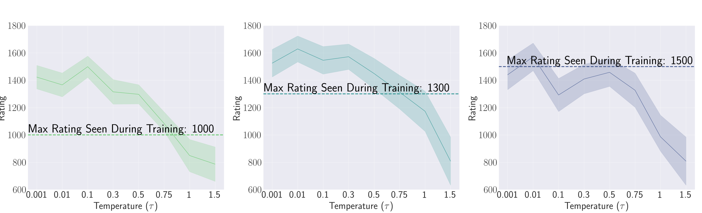
Figure 1: Ratings of our autoregressive decoder-only transformer, ChessFormer, over several different temperatures. We refer to our models as “ChessFormer <Maximum Glicko-2 rating seen during training>" to easily distinguish between different models in subsequent sections. Each model is trained only on games with players up to a certain rating ( $1000$ , $1300$ , $1500$ , respectively). We report 95% confidence intervals calculated through taking $± 1.96\sigma$ .
1 Introduction
Generative models (GMs) are typically trained to mimic human behavior. These humans may be skilled in their various human objectives: answering a question, creating art, singing a song. The model has only one objective: minimizing the cross-entropy loss with respect to the output distribution, thereby adjusting it to match the distribution of human labels Although chatbots are subject to a variety of post-training tuning methods, e.g., RLHF, we restrict our scope by assuming that the specialized knowledge and capacities are already provided by cross-entropy loss.. Therefore, one might assume the model can, at best, match the performance of an expert on their human objectives. Is it possible for these models to surpass—to transcend —their expert sources in some domains?
We illustrate an example of such transcendence in Figure 1, which measures the chess ratings (Glicko-2 [7]) of several transformer [35] models. Our experimental testbed is generative modeling on chess, which we choose as a domain for its well-understood, constrained nature. The transformer models are trained on public datasets of human chess transcripts, autoregressively predicting the next move in the game. To test for transcendence, we limit the maximal rating of the human players in the dataset below a specified score. We find that ChessFormer $1000$ and ChessFormer $1300$ (the latter number being the maximum rating seen during training) achieve significant levels of transcendence, surpassing the maximal rating seen in the dataset. Our focus is this capacity of a GM to transcend its expert sources by broadly outperforming any one expert. The key to our findings is the observation that GMs implicitly perform majority voting over the human experts. As these models are trained on a collection of many experts with diverse capacities, predilections, and biases, this majority vote oftentimes outperforms any individual expert, a phenomena that is known as “wisdom of the crowd”.
Our objective is to formalize the notion of transcendence and focus narrowly on this source of improvement over the experts: the removal of diverse human biases and errors. We prove that this form of denoising is enabled by low-temperature sampling, which implicitly induces a majority vote. Our result draws a subtle but deep connection from our new setting to a rich prior literature on model ensembling [1, 6, 19], enabling several key results. We precisely characterize the conditions under which transcendence is possible, and give a rigorous theoretical framework for enabling future study into the phenomenon. To test the predictive power of our theory, we then empirically demonstrate these effects. Digging deeper into the effects of majority voting, we show that its advantage is primarily due to performing much better on a small subset of states—that is, under conditions that are likely key to determining the outcome of the game. We also find that diversity in the data is a necessary condition for practically effective majority voting, confirming our theoretical findings. In short:
- We formalize the notion of transcendence in generative models (Section 2).
- We find a key insight explaining one cause of transcendence by connecting the case of denoising experts to model ensembling. In low temperature sampling settings, we prove that a generative model can transcend if trained on a single expert that makes mistakes uniformly at random. We then extend this result to transcending a collection of experts that are each skilled in different domains (Section 3).
- We train a chess transformer on game transcripts that only include players up to a particular skill level. We confirm our theoretical prediction that this model only surpasses the maximum rating of its expert data generators at low temperature settings (Section 4).
- We visualize the distribution of changes in reward by setting a lower sampling temperature, attributing the increased performance to large improvements on a relatively small portion of states (Section 4.2).
- We explore the necessity of dataset diversity, and the inability of ChessFormer to transcend when trained on less diverse datasets (Section 4.2).
2 Definition of Transcendence
Denote by $\mathcal{X}$ the (variable-length) input space and by $\mathcal{Y}$ the (finite) output space. Let $\mathcal{F}$ be the class of all functions mapping $\mathcal{X}\mapsto P(\mathcal{Y})$ (where we use the notation $P(\mathcal{Y})$ to denote probability distributions over $\mathcal{Y}$ ). That is, the functions in $\mathcal{F}$ map inputs in $\mathcal{X}$ to probability distributions over $\mathcal{Y}$ , so each function $f∈\mathcal{F}$ defines a conditional probability distribution of $y∈\mathcal{Y}$ given $x∈\mathcal{X}$ . We denote this distribution by $f(y|x)$ .
Fix some input distribution $p$ over $\mathcal{X}$ such that $p$ has full support (namely, for every $x∈\mathcal{X}$ we have $p(x)>0$ ). Throughout the paper, we assume that our data is labeled by $k$ experts, denoted $f_{1},...,f_{k}∈\mathcal{F}$ . Namely, we assume that the inputs are sampled from the input distribution $p$ and then each input $x∈\mathcal{X}$ is labeled by some expert chosen uniformly at random Equivalently, we can assume that each example is labeled by all experts.. This process induces a joint probability distribution over $\mathcal{X}×\mathcal{Y}$ , which we denote by $\operatorname*{D}$ . Specifically, $\operatorname*{D}(x,y)=p(x)\overline{f}(y|x)$ where $\overline{f}$ is the mixture of the expert distributions, namely
$$
\overline{f}(y|x)=\frac{1}{k}\sum_{i=1}^{k}f_{i}(y|x) \tag{1}
$$
We measure the quality of some prediction function $f∈\mathcal{F}$ using a reward assigned to each input-output pair. Namely, we define a reward function $r:\mathcal{X}×\mathcal{Y}→\mathbb{R}$ , s.t. for all $x$ , the function $r(x,·)$ is not constant (i.e., for every input $x$ not all outputs have the same reward). We choose some test distribution $p_{\mathrm{test}}$ over $\mathcal{X}$ , and for some $f∈\mathcal{F}$ define the average reward of $f$ over $p_{\mathrm{test}}$ by:
$$
R_{p_{\mathrm{test}}}(f)=\mathbb{E}_{x\sim p_{\mathrm{test}}}\left[r_{x}(f)%
\right],~{}~{}~{}\mathrm{where}~{}~{}r_{x}(f)=\mathbb{E}_{y\sim f(\cdot|x)}%
\left[r(x,y)\right] \tag{2}
$$
A learner has access to the distribution $\operatorname*{D}$ , and needs to find a function that minimizes the cross-entropy loss over $\operatorname*{D}$ . Namely, the learner chooses some function $\hat{f}∈\mathcal{F}$ s.t. $\hat{f}=\arg\min_{f∈\mathcal{F}}\mathbb{E}_{x\sim p}\left[H(\overline{f},f)\right]$ where $H$ is the cross-entropy function.
**Definition 1**
*We define “transcendence” to be a setting of $f_{1},...,f_{k}∈\mathcal{F}$ and $p∈ P(\mathcal{X})$ where:
$$
R_{p_{\mathrm{test}}}(\hat{f})>\max_{i\in[k]}R_{p_{\mathrm{test}}}(f_{i}) \tag{3}
$$*
In other words, transcendence describes cases where the learned predictor performs better (achieves better reward) than the best expert generating the data. Note that we are focusing on an idealized setting, where the learner has access to infinite amount of data from the distribution $\operatorname*{D}$ , and can arbitrarily choose any function to fit the distribution (not limited to a particular choice of architecture or optimization constraints). As we will show, even in this idealized setting, transcendence can be impossible to achieve without further modifying the distribution.
**Remark 1**
*We have made various simplifying assumptions when introducing our setting. For example, we assume that all experts share the same input distribution, we assume that all inputs have non-zero probability under the training distribution $p$ , and we assume the experts are sampled uniformly at random. We leave a complete analysis of a more general setting to future work, and discuss this point further in section 6.*
3 Conditions for Transcendence
In this section we analyze the necessary and sufficient conditions for transcendence in our setting. We begin by showing that low-temperature sampling is necessary for transcendence in our specific setting. Then, we analyze specific sufficient conditions for transcendence, both in the case where the data is generated by a single expert and when the data is generated by multiple experts. We defer all proofs to Appendix A.
<details>
<summary>extracted/5922169/advantage-analysis.png Details</summary>
### Visual Description
# Technical Document Extraction: Chess Reward Visualization Analysis
This document provides a comprehensive extraction of data and visual components from the provided image, which illustrates the relationship between a temperature parameter ($\tau$) and reward distributions in a chess-based reinforcement learning or decision-making context.
## 1. Image Overview and Structure
The image is organized into three vertical columns, each representing a different value for a temperature parameter $\tau$. Each column contains:
- **Top Section:** A chess board diagram showing a specific game state with highlighted squares and movement arrows.
- **Middle Section:** A label for the temperature parameter $\tau$.
- **Bottom Section:** A bar chart representing the probability or reward distribution for specific moves.
A vertical color legend is located on the far left of the image.
---
## 2. Global Components
### 2.1 Legend (Left Side)
- **Label:** "Reward $R_x(y)$" (Vertical text).
- **Spatial Placement:** $[x \approx 0.05, y \approx 0.35]$
- **Color Scale:** A vertical gradient bar ranging from dark blue (bottom) to deep magenta/maroon (top).
- **Function:** Maps the intensity of the reward/probability to specific colors used in the chess boards and bar charts.
### 2.2 Chess Board Configuration (Common to all boards)
- **Grid:** $8 \times 8$ squares.
- **Horizontal Axis (Files):** labeled 'a' through 'h'.
- **Vertical Axis (Ranks):** labeled '1' through '8'.
- **Key Pieces and Positions:**
- **White:** King on g2, Pawns on a2, e2, h2, b3, f3, g5, Rook on a1, f1, Bishop on c1, Knight on c3.
- **Black:** King on g8, Queen on c6, Rook on d4, f8, Knight on h5, Pawns on a7, b7, f7, g7, h7, d5.
- **White Queen:** Positioned on e7.
---
## 3. Segmented Analysis by Temperature ($\tau$)
### 3.1 Column 1: $\tau = 1.0$
- **Chess Board Visuals:**
- **Highlighted Squares:** Square **e8** is highlighted in deep magenta. Square **g6** is highlighted in blue. Square **g4** is highlighted in dark blue.
- **Movement Arrows:**
- Red arrow from Rook at f8 to e8.
- Red arrow from Queen at c6 to g6.
- Red arrow from Knight at h5 to f4/g4 area.
- Red arrow from Rook at d4 to f4.
- **Bar Chart Data:**
| Move Index | Move Description | Color | Approximate Value |
| :--- | :--- | :--- | :--- |
| 1 | Rook moving left (f8 to e8) | Magenta | 0.35 |
| 2 | Knight moving down-left (h5 to g4) | Blue | 0.22 |
| 3 | Queen moving right (c6 to g6) | Dark Blue | 0.15 |
| 4 | Rook moving right (d4 to f4) | Dark Blue | 0.05 |
### 3.2 Column 2: $\tau = 0.75$
- **Chess Board Visuals:** Similar to $\tau = 1.0$, but the color intensity of the highlighted squares (e8, g6, g4) is slightly more concentrated toward the top-ranked move.
- **Bar Chart Data:**
| Move Index | Move Description | Color | Approximate Value |
| :--- | :--- | :--- | :--- |
| 1 | Rook moving left (f8 to e8) | Magenta | 0.33 |
| 2 | Knight moving down-left (h5 to g4) | Blue | 0.15 |
| 3 | Queen moving right (c6 to g6) | Dark Blue | 0.10 |
| 4 | Rook moving right (d4 to f4) | Dark Blue | 0.08 |
### 3.3 Column 3: $\tau = 0.001$
- **Chess Board Visuals:**
- **Highlighted Squares:** Square **e8** is highlighted in deep magenta. The other squares (g6, g4) have lost their color highlights, indicating they are no longer considered viable under this temperature.
- **Movement Arrows:** Only the arrow from Rook f8 to e8 remains prominent/red.
- **Bar Chart Data:**
| Move Index | Move Description | Color | Approximate Value |
| :--- | :--- | :--- | :--- |
| 1 | Rook moving left (f8 to e8) | Magenta | 1.0 |
| 2 | Knight moving down-left (h5 to g4) | N/A | 0.0 |
| 3 | Queen moving right (c6 to g6) | N/A | 0.0 |
| 4 | Rook moving right (d4 to f4) | N/A | 0.0 |
---
## 4. Summary of Trends and Logic
- **Temperature Effect:** As the temperature $\tau$ decreases from $1.0$ to $0.001$, the "Reward" distribution shifts from a soft, exploratory distribution (where multiple moves have non-zero probability) to a hard, "winner-take-all" distribution.
- **Primary Move:** In all cases, the move **Rook from f8 to e8** (capturing or checking, indicated by the magenta highlight) is identified as the highest reward action.
- **Visual Encoding:** The color of the bars in the charts matches the color of the destination squares on the chessboards, providing a direct spatial-to-statistical mapping.
</details>
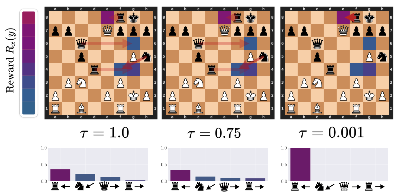
Figure 2: Visualizing the denoising effects of low temperature on the action distribution: an example of ChessFormer shifting probability mass towards the high reward move of trapping the queen with the rook as the temperature $\tau$ decreases. Opacity of the red arrows represent the probability mass given to different moves. The color of the square represent the reward that would be given for taking the action that moves the given piece to that state. Purple here is high reward, while blue is low. For more visualizations, see Appendix B.
3.1 Low-Temperature Sampling is Necessary for Transcendence
Observe that by definition of $\hat{f}$ , and using standard properties of the cross-entropy loss, we get that $\hat{f}=\overline{f}$ , as defined in Eq. (1). Therefore, the conditional probability distribution generated by $\hat{f}$ is simply an average of the distributions generated by the expert. Since the reward is a linear function of these distributions, we get that $\hat{f}$ never achieves transcendence:
**Proposition 1**
*For all choice of $f_{1},...,f_{k}$ and $p_{\mathrm{test}}$ , there exists some $f_{i}$ s.t. $R_{p_{\mathrm{test}}}(f_{i})≥ R_{p_{\mathrm{test}}}(\hat{f})$ .*
Note that in our setting, we assume that all experts are sampled uniformly for a given input $x$ . If instead this assumption is removed, then it may be possible to achieve transcendence with a bayesian weighting. We leave this analysis for future work.
3.2 Transcendence with Low-Temperature Sampling
Now, we consider a temperature sampling scheme over the learned function $\hat{f}$ . Namely, for some temperature $\tau>0$ , and some probability distribution $q∈ P(\mathcal{Y})$ , denote the softmax operator with temperature $\tau$ by $\mathrm{softmax}(q;\tau)∈ P(\mathcal{Y})$ s.t. $\mathrm{softmax}(q;\tau)_{y}=\dfrac{\exp(q_{y}/\tau)}{\sum_{y^{\prime}∈%
\mathcal{Y}}\exp(q_{y^{\prime}}/\tau)}$ . Additionally, we define $\operatorname*{arg\,max}(q)∈ P(\mathcal{Y})$ to be the uniform distribution over the maximal values of $q$ , namely $\operatorname*{arg\,max}(q)=1/{\left\lvert Y_{q}\right\rvert}$ if $y∈ Y_{q}$ and 0 if $y∉ Y_{q}$ , where $Y_{q}=\{y∈\mathcal{Y}:q_{y}=\max(q)\}$ . Now, define $\hat{f}_{\tau}$ to be the temperature sampling of $\hat{f}$ , i.e. $\hat{f}_{\tau}(·|x)=\mathrm{softmax}(\hat{f}(·|x);\tau)$ and $\hat{f}_{\max}$ the arg-max “sampling” of $\hat{f}$ , i.e. $\hat{f}_{\max}(·|x)=\operatorname*{arg\,max}(\hat{f}(·|x))$ . We now show that if the arg-max predictor $\hat{f}_{\max}$ is better than the best expert, then transcendence is possible with low-temperature sampling.
**Proposition 2**
*$R_{p_{\mathrm{test}}}(\hat{f}_{\max})>\max_{i∈[k]}R_{p_{\mathrm{test}}}(f_{i})$ if and only if there exists some temperature $\tau∈(0,1)$ s.t. for all $0≤\tau^{\prime}≤\tau$ , it holds that $R_{p_{\mathrm{test}}}(\hat{f}_{\tau^{\prime}})>\max_{i∈[k]}R_{p_{\mathrm{%
test}}}(f_{i}).$*
The above shows that, even though transcendence cannot be achieved when directly modeling the distribution, it can be achieved by temperature sampling, assuming that the arg-max predictor achieves higher reward compared to all experts. In other words, we make the subtle connection here that low-temperature sampling can be thought of as performning majority vote [1, 6] between the experts. Please see Appendix A for a formal proof of this connection. When the experts put non-negligible mass onto the best actions, the resulting majority vote may find the best action [9], which improves performance compared to individual experts (i.e., “wisdom of the crowd”) and thus achieve transcendence.
3.3 Denoising a Single Expert
We now turn to study particular cases where low-temperature sampling can lead to transcendence. The most simple case is of a single expert that outputs a correct but noisy prediction. Denote by $f^{*}$ the optimal expert, s.t. for all $x$ we have $f^{*}(y|x)=\dfrac{\delta(y∈ Y^{*}_{x})}{\lvert Y^{*}_{x}\rvert}$ , where $Y^{*}_{x}=\{y∈\mathcal{Y}:y=\max_{y^{\prime}}r(x,y^{\prime})\}$ and $\delta(\text{condition})$ is 1 if the condition is true and 0 otherwise. Now, for some $\rho∈(0,1)$ , let $f_{\rho}$ be a “noisy” expert, s.t., for all $x$ , with probability $\rho$ chooses a random output, and with probability $1-\rho$ chooses an output according to the optimal expert $f^{*}(·|x)$ , namely $f_{\rho}(y|x)=\rho/\left\lvert\mathcal{Y}\right\rvert+(1-\rho)f^{*}(y|x)$ . We show that transcendence is achieved with low-temperature sampling for data generated by $f_{\rho}$ :
**Proposition 3**
*Assume the data is generated by a single expert $f_{\rho}$ . Then, there exists some temperature $\tau∈(0,1)$ s.t. for all $\tau^{\prime}≤\tau$ , the predictor $\hat{f}_{\tau^{\prime}}$ achieves “transcendence”.*
3.4 Transcendence from Multiple Experts
Next, we consider the case where the dataset is generated by multiple experts that complement each other in terms of their ability to correctly predict the best output. For example, consider the case where the input space is partitioned into $k$ disjoint subsets, $\mathcal{X}=\mathcal{X}_{1}\dot{\cup}...\dot{\cup}\mathcal{X}_{k}$ , s.t. the $i$ -th expert performs well on the subset $\mathcal{X}_{i}$ , but behaves randomly on other subsets. Namely, assume the expert $f_{i}$ behaves as follows: $f_{i}(y|x)=\biggl{(}\frac{\delta(y∈ Y^{\star}_{x})\delta(x∈\mathcal{X}_{i}%
)}{|Y^{\star}_{x}|}+\frac{\delta(x∉\mathcal{X}_{i})}{|\mathcal{Y}|}\biggr%
{)}$ where $Y_{x}^{*}$ is as previously defined and $\delta(\text{condition})$ is 1 if the condition is true and 0 otherwise. We show that, assuming that the test distribution $p_{\mathrm{test}}$ is not concentrated on a single subset $\mathcal{X}_{i}$ , we achieve transcendence with low-temperature sampling:
**Proposition 4**
*Let $p_{\mathrm{test}}$ be some distribution s.t. there are at least two subsets $\mathcal{X}_{i}≠\mathcal{X}_{j}$ s.t. $p_{\mathrm{test}}(\mathcal{X}_{i}),p_{\mathrm{test}}(\mathcal{X}_{j})>0$ . Then, if the data is generated by $f_{1},...,f_{k}$ , there exists some temperature $\tau∈(0,1)$ s.t. for all $\tau^{\prime}≤\tau$ , the predictor $\hat{f}_{\tau^{\prime}}$ achieves “transcendence”.*
In order to build intuition for Proposition 4, see Appendix C for an intuitive diagram.
4 Experiments
To evaluate the predictive power of our impossibility result of transcendence with no temperature sampling (Proposition 1) as well as our result of transcendence from multiple experts with low temperature sampling (Proposition 2), we turn to modeling and training chess players. Chess stands out as an attractive option for several reasons. Chess is a well-understood domain and more constrained than other settings such as natural language generation, lending to easier and stronger analysis. Evaluation of skill in chess is also natural and well-studied, with several rigorous statistical rating systems available. In this paper, we use the Glicko-2 rating system [7], which is also adopted by https://lichess.org, the free and open-source online chess server from which we source our dataset.
4.1 Experimental Setup
<details>
<summary>extracted/5922169/latent_board_state_reward_tsne.png Details</summary>
### Visual Description
# Technical Document Extraction: Chess Reward Visualization
## 1. Document Overview
This image is a technical visualization, likely from a machine learning or reinforcement learning research paper, illustrating a latent space mapping of chess positions. It utilizes a dimensionality reduction technique (such as t-SNE or UMAP) to project high-dimensional chess states into a 2D plane, colored by a "Reward" metric.
---
## 2. Component Isolation
### Region A: Main Scatter Plot (Top)
* **Type:** 2D Scatter Plot / Heatmap.
* **Content:** A dense collection of data points representing individual chess positions.
* **Spatial Distribution:** The points are clustered into various "islands" or groupings, suggesting that the model has learned to group similar chess positions together in its latent space.
* **Color Gradient:** The points are colored based on a continuous scale.
* **Red/Magenta:** High density of high-reward positions.
* **Blue/Teal:** High density of low-reward positions.
* **Purple:** Intermediate reward values.
### Region B: Legend (Right Side)
* **Location:** [x: ~90%, y: ~40%]
* **Title:** "Reward" (oriented vertically).
* **Scale Type:** Continuous color bar.
* **Markers:**
* **1.0:** Bright Red (Top)
* **0.75:** Magenta
* **0.5:** Purple (Middle)
* **0.25:** Dark Blue
* **0.0:** Teal/Cyan (Bottom)
### Region C: Callout Examples (Bottom)
Four specific chess board configurations are pulled from the main plot via dashed lines to show the relationship between board state and the calculated reward value ($\mathbb{E}_{y \sim f^*}[r_x]$).
---
## 3. Data Extraction: Callout Boards
| Board Index (Left to Right) | Reward Value ($\mathbb{E}_{y \sim f^*}[r_x]$) | Visual Color Correlation | Key Board Features |
| :--- | :--- | :--- | :--- |
| **Board 1** | **1.0** | Red (High) | Endgame state. White has a significant material advantage (Queen, Knight, Bishop, Pawn) against a lone Black King. |
| **Board 2** | **0.0** | Teal (Low) | Endgame state. Black has a significant material advantage (Two Queens, two Bishops) against a lone White King. |
| **Board 3** | **0.53** | Purple (Mid) | Opening/Midgame state. Standard development (e.g., Ruy Lopez or Italian Game variation). Symmetrical material. |
| **Board 4** | **0.54** | Purple (Mid) | Opening/Midgame state. Similar to Board 3, showing a standard development phase with balanced material. |
---
## 4. Mathematical Notation
The image contains the following LaTeX-style mathematical expression beneath each board:
$$\mathbb{E}_{y \sim f^*}[r_x]$$
* **$\mathbb{E}$**: Expected value operator.
* **$y \sim f^*$**: Indicates that $y$ is sampled from the optimal distribution or ground truth function $f^*$.
* **$r_x$**: The reward associated with state $x$.
* **Interpretation:** This represents the expected reward of a given chess position $x$ under an optimal policy or ground truth evaluator.
---
## 5. Trend Analysis and Observations
1. **Clustering by Game Phase:** The scatter plot shows distinct clusters. The callouts suggest that the large, dense cluster on the left contains endgame positions (extreme rewards of 0.0 or 1.0), while the smaller clusters on the right represent opening or midgame positions (neutral rewards around 0.5).
2. **Reward Polarity:** The visualization effectively separates "winning" positions (Red) from "losing" positions (Teal) for the perspective being evaluated (presumably White).
3. **Spatial Grounding Logic Check:**
* The dashed line from **Board 1 (Reward 1.0)** points to a bright **Red** region in the far-left cluster.
* The dashed line from **Board 2 (Reward 0.0)** points to a **Teal** region within the same far-left cluster.
* The dashed lines from **Boards 3 and 4 (Rewards ~0.5)** point to **Purple** clusters on the right side of the map.
* *Verification:* The colors of the target regions in the scatter plot match the legend values and the numerical labels provided under the boards.
</details>
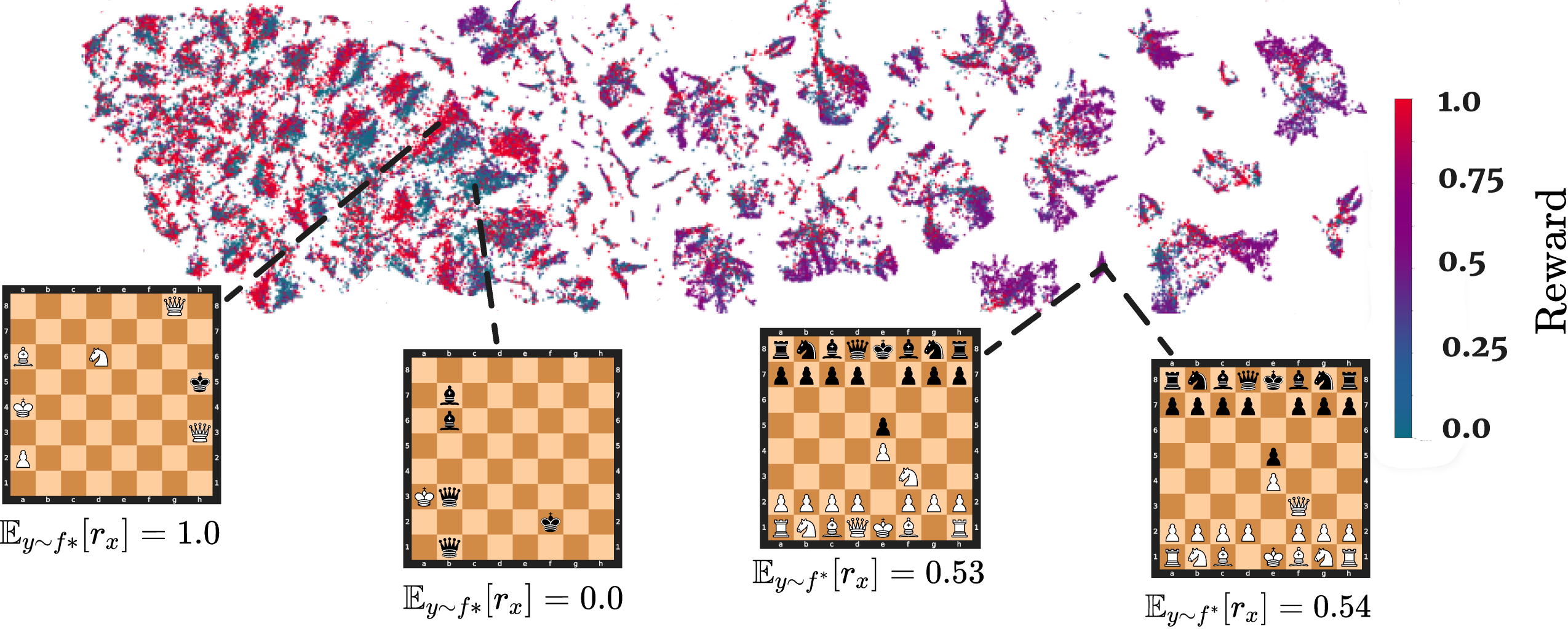
Figure 3: Inspired by Mnih et al. [20], we generate a t-SNE embedding [34] of ChessFormer’s last hidden layer latent representations of game transcripts during training time. The colors represent the probability of winning, with $+1$ corresponding to a state where White has won and $0 0$ to Black. Probabiliy of winning is computed through the Stockfish analysis engine. We also visualize several board states associated with different clusters in the t-SNE embedding, and their associated expected reward when following the expert Stockfish distribution. Note that the model distinguishes between states where the outcome has already been determined (the two left boards), versus opening states that are extremely similar (the two right boards). See the full t-SNE in Appendix G.
Training Details.
We trained several $50$ M parameter autoregressive transformer decoders following best practices from modern large model training, including a cosine learning rate schedule and similar batch size-learning rate ratios as prescribed by the OPT-175B team [37]. Our dataset consists of human chess games from the lichess.org open source database from January 2023 to October 2023. In total, this dataset contains approximately one billion games. In this setting, an expert is a specific individual player. To test for transcendence, we truncate this dataset by a maximum rating, so that during training a model only sees data up to a given rating. We train our model on the next-token prediction objective, and represent our chess games as Portable Game Notation (PGN) strings, such as 1.e4 e5 2.Nf3 Nc6 3.Bb5... 1/2-1/2. Note that we do not give any rating or reward information during training—the only input the model sees are the moves and the outcome of the game. We tokenize our dataset at the $32$ -symbol character level. (For further details, see Appendix E.) Our model plays chess “blind”—without direct access to the board state—and, furthermore, is never explicitly given the rules of the game: at no point is play constrained to valid outputs for a given piece or board state. Nontrivial chess skill is therefore not straightforward to acquire, and if not for the surprising capabilities of modern large transformers, one might imagine such a model would fail to learn even the basic rules of playing chess. This blindfolded setting has also been studied by prior work [23, 30], as discussed further in section 5.
One gap between our theory and practice is that in our theory, we assume that each expert is defined over the entire input space $\mathcal{X}$ . However, in the chess setting such full coverage is extremely unlikely to be the case after around move $15$ , as there are more unique chess games than atoms in the universe due to the high branching factor of the game tree. To address this gap, we visualize the latent representation of our model in Figure 3, where we find the model is able to capture meaningful semantics regarding both the relative advantage of a state, as well as the identity of the black and white player. This visualization illustrates the ability of our model to generalize by compressing games into some shared latent representation, enabling experts to generalize to unseen states, bridging this gap between theory and practice.
Evaluation.
We evaluate each model by its Glicko-2 ratings against Stockfish 16.1 [29], a popular open-source chess engine. Stockfish uses a traditional minimax search equipped with a bespoke CPU-efficient neural network for evaluation [22] and $\alpha$ - $\beta$ pruning for further efficiency. We evaluate Stockfish at levels 1, 3, and 5 with a 100ms timeout directly on Lichess’ platform against the Maia [18] 1, 5, and 9 bots (human behavior cloned convolutional networks trained at rating bins 1100-1200, 1500-1600, and 1900-2000, respectively) for several hundred games, obtaining calibrated Glicko-2 ratings for Stockfish specifically on Lichess’ platform ( $1552± 45.2$ , $1842± 45.2$ , $2142± 59$ for Stockfish Levels 1, 3, and 5, respectively). Next, for evaluating our own models, we then play against Stockfish levels of 1, 3, and 5 for 100 games each, reaching a final rating calculation with 300 games. We then report both the Glicko-2 rating $R$ as well as rating deviation $RD$ of our models, where $R± 2*RD$ provides a $95\%$ confidence interval. To play against Stockfish, we successively prompt our model with the current game PGN string. Note that our output is entirely unconstrained, and may be either illegal in the current board state or altogether unparsable. If our model fails to generate a valid legal move after 5 samples, we consider it to have lost. After generation, we give the updated board state to Stockfish and pass a new PGN string appended with the prior move of Stockfish back to our model. We repeat this process until the game ends.
4.2 Experimental Results
Main Result: Low-temperature sampling enables transcendence.
In this section we attempt to answer our primary research question, can low-temperature sampling actually induce transcendence in practice? We test Proposition 2 by evaluating several ChessFormers across different temperature values, from $0.001$ (nearly deterministic), to $1.0$ (original distribution), to $1.5$ (high entropy). In Figure 1 we definitively confirm the existence of transcendence. Our ChessFormer 1000 (where the latter number refers to the maximum rating seen during training) and ChessFormer 1300 models are able to transcend to around 1500 rating at temperature $\tau$ equal to $0.001$ . Interestingly, ChessFormer 1500 is unable to transcend at test time, a result we further analyze in Dataset Diversity.
To more deeply understand when and why transcendence occurs, we investigate two questions. (1) How does the reward function defined in Equation 2 shift with respect to low-temperature sampling? (2) Does transcendence rely on dataset diversity, as introduced theoretically in subsection 3.4?
Lowering temperature increases rewards in expectation on specific states, leading to transcendence over the full game.
When playing chess, a low-skilled player may play reasonably well until they make a significant blunder at a key point in play. If these errors are idiosyncratic, averaging across many experts would have a denoising effect, leaving the best moves with higher probability. Therefore, low-temperature sampling would move probability mass towards better moves in specific play contexts. Without low-temperature sampling, the model would still put probability mass onto blunders. To gain intuition for this idea, we visualize it theoretically in Appendix C and empirically in Figure 2 and Appendix B. This hypothesis motivates our first research question in this section: Does low-temperature sampling improve the expected reward very much for just some specific key game states, or a little for many game states?
To formalize this notion, we first define a “favor” function, which captures the improvement in reward by following some new probability distribution over some baseline probability distribution. Our definition is inspired by the Performance Difference Lemma (PDL) [10] from Reinforcement Learning (RL), which establishes an equivalence between the change in performance from following some new policy (a probability distribution of actions given a state) over some old policy, and the expected value of the advantage function of the old policy sampled with respect to the new policy. In RL, the advantage function is defined as the difference between the value of taking a single action in a given state versus the expected value of following some policy distribution of actions in that state.
Here, we define the “favor” of $f^{\prime}$ over $f$ in $x$ as the change in the reward function by comparing what $f$ would have done when following $f^{\prime}$ for a given input $x$ :
$$
F(f^{\prime},f;x)=\mathbb{E}_{x\sim d^{f^{\prime}},y\sim f^{\prime}(\cdot|x)}[%
r(x,y)]-\mathbb{E}_{x\sim d^{f^{\prime}},y\sim f(\cdot|x)}[r(x,y)]. \tag{4}
$$
Where $d^{f}$ refers to the state visitation distribution [31] when following $f$ in a sequential setting—informally, this variable can be thought of the distribution of states seen when sampling from $f$ with a fixed transition function that takes in an input $x$ , a output $y$ , and outputs a next input $x$ . Here, that transition function is given by the rules of chess and the opponent player. Given this favor function, we can now quantitatively explore the effects that lead to transcendence by setting the baseline $f$ to be the original imitation-learned probability distribution (temperature $\tau=1$ ), and $f^{\prime}$ as a low-temperature intervention on $f$ (e.g. temperature $\tau=0$ ). We can empirically calculate the reward by using the evaluation function [22] of Stockfish, an expert neural reward function that Stockfish uses to calculate its next move. This reward function is a neural network trained to predict the probability of winning through a sigmoid on a linear combination of handcrafted expert heuristics, such as amount of material versus opponent material, and number of moves to a potential checkmate.
<details>
<summary>extracted/5922169/adv-gain-dist-flat.png Details</summary>
### Visual Description
# Technical Document Extraction: Probability Distribution Analysis
## 1. Component Isolation
* **Header/Legend:** Located in the top-left quadrant of the plot area.
* **Main Chart:** A histogram plot with overlapping distributions and vertical indicator lines.
* **X-Axis:** Horizontal axis at the bottom representing numerical change values.
* **Y-Axis:** Vertical axis on the left representing probability density.
---
## 2. Metadata and Axis Labels
* **Y-Axis Title:** $\mathbb{P}(F')$
* **Y-Axis Markers:** $[0.0, 0.2, 0.4, 0.6]$
* **X-Axis Title:** Change in expected reward over base $f_{\tau=1}$ probability distribution over individual states: $F(f', f)$
* **X-Axis Markers:** $[-10.0, -7.5, -5.0, -2.5, 0.0, 2.5, 5.0, 7.5, 10.0]$
---
## 3. Legend Extraction [Spatial Grounding: Top-Left]
The legend contains five entries, cross-referenced with the visual elements in the chart:
| Legend Icon | Label | Description |
| :--- | :--- | :--- |
| Light Green Box | $f' = f_{\tau=0.001}$ | Distribution for a very low temperature parameter. |
| Light Red Box | $f' = f_{\tau=0.75}$ | Distribution for a moderate temperature parameter. |
| Black Line | Baseline $\mathbb{E}[F] : 0.0$ | Vertical reference line at $x = 0.0$. |
| Green Line | $\mathbb{E}[F] : 2.15$ | Expected value for the green distribution. |
| Red Line | $\mathbb{E}[F] : 0.99$ | Expected value for the red distribution. |
---
## 4. Data Series Analysis and Trends
### Series 1: $f' = f_{\tau=0.001}$ (Light Green Histogram)
* **Visual Trend:** This distribution is highly "heavy-tailed" to the right. While it has a peak near zero, it maintains a significant, low-level density stretching far into the positive x-range (up to 10.0 and likely beyond).
* **Central Tendency:** Indicated by the **Green Vertical Line** at $x = 2.15$.
* **Observation:** The spread is much wider than the red distribution, indicating higher variance in the change of expected reward.
### Series 2: $f' = f_{\tau=0.75}$ (Light Red Histogram)
* **Visual Trend:** This distribution is much more concentrated (peaked) around the zero point. It drops off significantly faster than the green distribution as $x$ increases.
* **Peak Height:** The highest bin is located just to the right of $0.0$, reaching a probability density of approximately $0.65$.
* **Central Tendency:** Indicated by the **Red Vertical Line** at $x = 0.99$.
* **Observation:** This represents a more conservative shift compared to the $\tau=0.001$ setting.
### Overlap (Tan/Brown Areas)
* Where the red and green histograms overlap, the color appears as a muted tan. The highest concentration of overlap is between $x = 0.0$ and $x = 2.5$.
---
## 5. Key Data Points and Indicators
* **Baseline:** A solid black vertical line is fixed at **0.0**, representing the reference point for "no change."
* **Red Mean ($\mathbb{E}[F]$):** Located at **0.99**. It sits within the primary mass of the red histogram.
* **Green Mean ($\mathbb{E}[F]$):** Located at **2.15**. Despite the green histogram having a lower peak than the red one near zero, its long right tail pulls the expected value significantly further to the right.
* **Range:** The data shown spans from approximately $-7.5$ to $10.0$, though the bulk of the probability mass for both distributions is located in the $[0.0, 5.0]$ range.
</details>
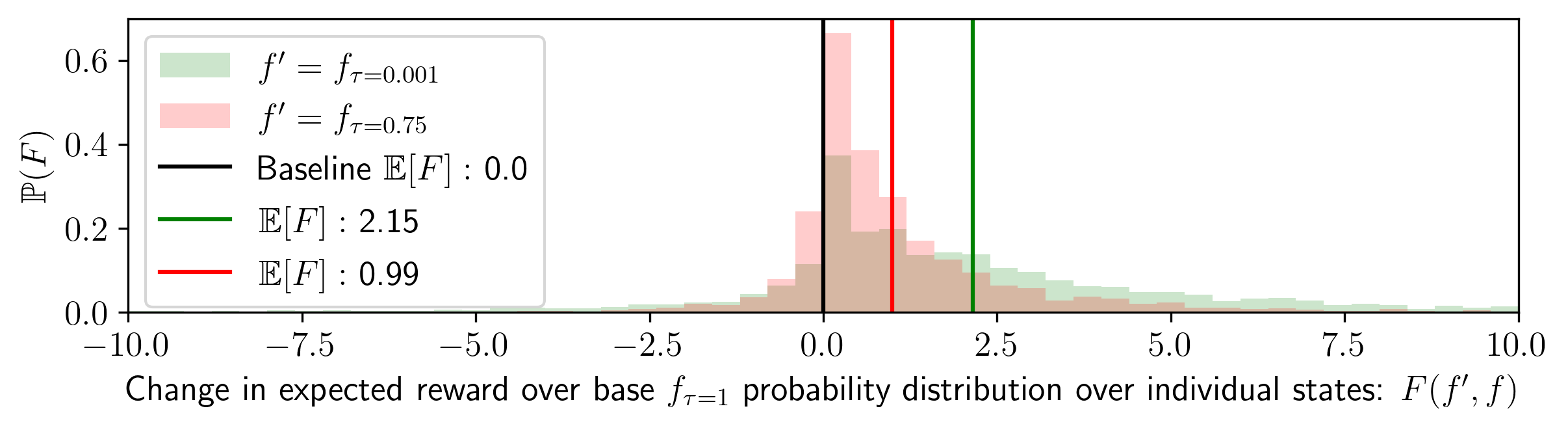
Figure 4: The favor probability distribution, or change in expected reward by setting temperature lower than $\tau=1.0$ . We plot the favor distribution across two different temperatures: setting $\tau=.75$ and $\tau=0.001$ by running the Stockfish analysis engine across $100$ total Chessformer $1000$ games played at $0.001$ temperature against Stockfish level $1$ (as theoretically justified by PDL [10]). We calculate favor by sampling $100$ counterfactual potential moves at $\tau=1.0$ per actual move made at $\tau=0.001$ to compute a baseline expected reward. In total, we gather an empirical probability distribution with $n=382,000$ total samples per $\tau$ ( $38.2$ moves on average per game). Note that we plot the distributions with transparency, so the brownish area is where the two overlap. We visualize several long-tail examples in Appendix B.
In Figure 4, we find that lowering the temperature has the effect of skewing the expected reward distribution to the right, especially for the green $\tau=0.001$ distribution. This result implies that the model does not improve the expected reward by a small amount for many game states, but rather improves the expected reward by a relatively large amount for a few game states. Thus, $\tau=0.001$ improves the expected reward (probability of winning) by an average of $\mathbf{2.15± 0.17\%}$ , but for some states, this expected improvement is over 5%. Note that the original temperature expected reward can be thought of as a Dirac distribution centered at $0 0$ . The above finding answers our research question in this section: Low-temperature sampling is able improves the expected reward by relatively large amounts for some specific game states, which is likely why the ChessFormer $1000$ and $1300$ model was able to achieve transcendence.
| $\tau=0.001$ | $\mathbf{39.95± 0.92}$ | $\mathbf{2.15± 0.17}$ | $\mathbf{29.61± 1.43}$ | $\mathbf{54.26± 1.57}$ | $\mathbf{66.86± 1.47}$ |
| --- | --- | --- | --- | --- | --- |
| $\tau=0.75$ | $38.79± 0.90$ | $0.99± 0.06$ | $25.08± 0.95$ | $47.84± 1.09$ | $60.37± 1.04$ |
| $\tau=1.0$ | $37.80± 0.87$ | $0± 0$ | $22.61± 0.86$ | $44.00± 9.96$ | $56.27± 0.93$ |
Table 1: Table of several statistics describing the relationship between reward at $\tau=0$ vs. $\tau=1$ . In the first column, we display the expected reward across our dataset, which is $\mathbb{P}$ of winning calculated by Stockfish 16.1). In the second column, we display $F$ , or the change in reward for the given temperature $\tau$ versus the baseline. In the last three columns we display the accuracy for the best moves ranked by Stockfish analysis run at a time cutoff of $1$ second. Here, the top- $k$ accuracy is the percentage of games where the actual move sampled by the model was in the top- $k$ moves as ranked by Stockfish. We report 95% bootstrapped confidence intervals with 10K resamples.
In Table 1, we present the statistics of the favor function for different temperature values. From this table, we observe that as the temperature decreases, the top- $k$ accuracies monotonically increase, suggesting that the model becomes more consistent in selecting good moves. We also observe that although the model improves as temperature decreases, the probability of winning is still below $50\%$ , meaning our model should tend to lose more games than it wins against Stockfish $1$ . This result matches with our results in Figure 1, as the rating of Stockfish $1$ is also higher than the reported rating for $\tau=0.001$ ( $1550$ for Stockfish 1 vs $\sim 1450$ for Chessformer $1000$ ). Overall, the analysis of the advantage statistics provides further evidence for the effectiveness of low-temperature sampling in inducing transcendence in chess models.
Dataset diversity is essential for transcendence.
As we note in subsection 3.4, our theory requires dataset diversity as a necessary condition for enabling transcendence. Importantly, we find in Figure 1 that not all models are able to transcend. Unlike ChessFormer 1000 or 1300, the Chessformer 1500 fails to transcend. We hypothesize that this results is due to the fact that in the band of ratings from $1000$ to $1500$ , diversity does not significantly increase. If so, a $1000$ rated player can be thought of as a noisy $1500$ rated player, but a $1500$ rated player cannot be thought of as a noisy $2000$ rated player. In this section we ask the following research question: Is diversity in data required for enabling transcendence?
In Figure 5, we explore this research question by quantifying dataset diversity through the normalized entropy on the action distribution $\mathcal{H}_{f}(Y|X)={\mathbb{E}_{y\sim f(y|x=X)}[-\log_{2}f(y|x=X)]}/{\log_{2%
}|\mathcal{Y}|}.$ To gain intuition for this metric, imagine the action distribution of moves taken for any given state. Entropy will be higher for more uniform action distributions, and lower for more deterministic, peaked action distributions. The average entropy of these action distributions can therefore serve as a measurement of the diversity of the dataset. We normalize this entropy to the range $[0,1]$ by dividing by the binary log of the number of legal moves: $\log_{2}|\mathcal{Y}|$ .
Importantly, we cannot calculate this normalized entropy for every state, as most states after move $16$ in the midgame and before the engame are unique within the dataset and we therefore observe just a single action for thus states. Therefore our metric is limited in that it only considers opening moves, the beginning of the midgame, and the endgame. We consider only common states with greater than $100$ actions by sampling $1,000,000$ games from each dataset. The average entropy confirm our hypothesis: The $<1500$ cut off dataset has on average less diversity than the $<1300$ dataset, which has is again less than the $<1000$ dataset. This result suggests that Chessformer $1500$ likely is not transcendent due to a lack of diversity in its dataset. If the entropy instead stayed constant for each dataset, it would imply that each had a similar level of diversity. In such a case, we would expect that ChessFormer $1500$ likely would also transcend. Instead, as predicted, it is likely not transcendent due to a lack of diversity.
<details>
<summary>x2.png Details</summary>
### Visual Description
# Technical Document Extraction: Entropy of Action Distribution
## 1. Header Information
* **Title:** $\mathcal{H}$ of action distribution over common states
* **Language:** English with mathematical notation (LaTeX).
## 2. Component Isolation
### Region A: Axis Labels and Markers
* **Y-Axis Title:** $\mathbb{P}(\mathcal{H}(Y|X))$
* *Description:* Represents the probability density or frequency of specific entropy values.
* *Markers:* 0.00, 0.05, 0.10, 0.15
* **X-Axis Title:** $\mathcal{H}(Y|X)$
* *Description:* Represents the conditional entropy of action $Y$ given state $X$.
* *Markers:* 0.0, 0.2, 0.4, 0.6, 0.8, 1.0
### Region B: Legend [Top-Left Placement]
The legend identifies three distinct data series based on "Max Rating," which likely refers to player skill levels in a game (e.g., Chess).
* **Green (Light/Transparent):** Max Rating: 1000
* **Orange/Yellow (Light/Transparent):** Max Rating: 1300
* **Red/Pink (Light/Transparent):** Max Rating: 1500
### Region C: Main Chart (Overlaid Histograms)
The chart consists of three overlapping histograms showing the distribution of entropy. All three distributions are negatively skewed (left-skewed), with the bulk of the data concentrated between 0.6 and 0.8 on the x-axis.
* **Trend Analysis:**
* **Max Rating 1000 (Green):** This distribution is shifted furthest to the right. It has the highest peak (mode) around 0.75.
* **Max Rating 1300 (Orange):** This distribution is centered slightly to the left of the 1000 rating group.
* **Max Rating 1500 (Red):** This distribution is shifted furthest to the left compared to the others, indicating lower average entropy.
### Region D: Statistical Annotations (Vertical Lines and Text)
The chart includes vertical lines representing the Expected Value (Mean), denoted as $\mathbb{E}[\mathcal{H}]$.
| Series (Max Rating) | Color of Line | Expected Value ($\mathbb{E}[\mathcal{H}]$) | Visual Position |
| :--- | :--- | :--- | :--- |
| **1000** | Green (Thick) | **0.70** | Furthest right vertical line |
| **1300** | Orange (Thin) | **0.66** | Middle vertical line |
| **1500** | Red (Thin) | **0.64** | Furthest left vertical line |
## 3. Data Summary and Key Findings
* **Inverse Correlation:** There is a clear inverse relationship between "Max Rating" and the entropy ($\mathcal{H}$) of the action distribution. As the player rating increases (from 1000 to 1500), the expected entropy decreases (from 0.70 to 0.64).
* **Interpretation:** In technical terms, higher-rated players (1500) have a more predictable action distribution (lower entropy) over common states compared to lower-rated players (1000), who exhibit higher entropy (more uncertainty or variety in action selection).
* **Distribution Overlap:** While the means are distinct, there is significant overlap between all three groups, particularly in the 0.5 to 0.9 entropy range. All groups show very low probability for entropy values below 0.2.
</details>
Figure 5: Action distribution diversity, as measured by the average normalized entropy over different chess rating dataset cutoffs with $n=2681,3037,3169$ common states for ratings $1000,1300,1500$ , respectively. These entropies are calculated directly from the empiricial frequencies of our dataset, and are model-agnostic.
4.3 Additional Settings
SQuADv2 Natural Language Temperature Denoising Experiment. We extend our analysis to the Natural Language Processing domain by running experiments on the Stanford Question Answering Dataset (SQuAD 2.0). We tested the effects of temperature denoising on the performance of several large language models (LLMs) of varying sizes. The SQuAD task involves reading comprehension and question-answering based on Wikipedia articles, making it an ideal setting to evaluate the impact of denoising on language models. We measured the exact-match, semantic-match, and F1 scores of the model outputs at different temperatures. The results show that temperature denoising leads to improved performance, corroborating the findings of our chess experiments and providing broader validation of the underlying mechanism of temperature denoising in diverse domains.
<details>
<summary>extracted/5922169/nlu_experiment/Combined_SQuADv2_Evaluation_Metrics_Broken_Axis.jpeg Details</summary>
### Visual Description
# Technical Data Extraction: Performance Metrics vs. Temperature
This document provides a comprehensive extraction of data from a series of three line charts comparing the performance of four Large Language Models (LLMs) across varying temperature settings.
## 1. General Metadata and Structure
The image consists of three sub-plots arranged horizontally. Each plot shares a common X-axis and legend but measures a different performance metric. All plots utilize a "broken" Y-axis to show the high-performing models (top section) and the significantly lower-performing GPT-2 model (bottom section) on the same scale.
### Common Legend
The legend is located in the lower-left quadrant of each main plot area.
* **Light Green:** Qwen2 (7B)
* **Teal/Medium Green:** Mistral (7B)
* **Steel Blue:** Gemma 2 (2B)
* **Dark Purple/Navy:** GPT-2 (163M)
### Common X-Axis
* **Title:** Temperature ($\tau$)
* **Markers:** 0.001, 0.25, 0.5, 0.75, 1, 1.5
---
## 2. Chart 1: F1 Score vs Temperature
### Axis Information
* **Y-Axis Title:** F1 Score
* **Y-Axis Markers (Top):** 30, 40, 50, 60, 70
* **Y-Axis Markers (Bottom):** 0, 5
### Data Trends and Values
All models exhibit a **downward trend** as temperature increases, indicating that higher stochasticity reduces F1 performance.
| Model | Trend Description | Approx. Value at $\tau=0.001$ | Approx. Value at $\tau=1.5$ |
| :--- | :--- | :---: | :---: |
| **Qwen2 (7B)** | Highest performer; steady slight decline. | 70 | 60 |
| **Mistral (7B)** | Second highest; parallel decline to Qwen2. | 65 | 52 |
| **Gemma 2 (2B)** | Third highest; steady decline. | 51 | 40 |
| **GPT-2 (163M)** | Significantly lower; slight decline. | 6 | 4 |
---
## 3. Chart 2: Exact Match (%) vs Temperature
### Axis Information
* **Y-Axis Title:** Exact Match (%)
* **Y-Axis Markers (Top):** 30, 40, 50, 60
* **Y-Axis Markers (Bottom):** 0, 1
### Data Trends and Values
All models exhibit a **downward trend**. The performance gap between the 7B models and the 2B/163M models is more pronounced here than in the F1 chart.
| Model | Trend Description | Approx. Value at $\tau=0.001$ | Approx. Value at $\tau=1.5$ |
| :--- | :--- | :---: | :---: |
| **Qwen2 (7B)** | Leading; sharpest drop after $\tau=0.5$. | 62% | 50% |
| **Mistral (7B)** | Second; steady decline. | 57% | 41% |
| **Gemma 2 (2B)** | Third; notable drop between 0.5 and 1.0. | 43% | 31% |
| **GPT-2 (163M)** | Near zero; negligible performance. | 0.4% | 0.0% |
---
## 4. Chart 3: Semantic Match (%) vs Temperature
### Axis Information
* **Y-Axis Title:** Semantic Match (%)
* **Y-Axis Markers (Top):** 30, 40, 50, 60, 70
* **Y-Axis Markers (Bottom):** 0, 5
### Data Trends and Values
The top three models show a **consistent downward trend**. GPT-2 shows a **volatile/flat trend** at a very low baseline.
| Model | Trend Description | Approx. Value at $\tau=0.001$ | Approx. Value at $\tau=1.5$ |
| :--- | :--- | :---: | :---: |
| **Qwen2 (7B)** | Highest; maintains >60% throughout. | 71% | 61% |
| **Mistral (7B)** | Second; steady decline. | 67% | 55% |
| **Gemma 2 (2B)** | Third; steady decline. | 52% | 43% |
| **GPT-2 (163M)** | Low/Flat; slight peak at $\tau=0.5$. | 6% | 5% |
---
## 5. Component Isolation Summary
* **Header:** Contains three distinct titles: "F1 Score vs Temperature", "Exact Match (%) vs Temperature", and "Semantic Match (%) vs Temperature".
* **Main Chart Area:** Features shaded regions around each line, representing confidence intervals or standard deviation. The background uses a light grey grid.
* **Footer:** Contains the X-axis labels "Temperature ($\tau$)" and the numerical scale.
* **Visual Indicators:** Diagonal "break" marks (//) are present on the Y-axes of all three charts between the 5/30 or 1/30 marks to indicate the scale discontinuity.
</details>
Figure 6: We evaluate several pretrained language models on the SQuADv2 Question-Answering reading comprehesion dataset, a task consisting of answering a question given some snippet from a Wikipedia article. We report F1, ’Exact Match’, and ’Semantic Match’ scores of several different language models of varying size from 163M parameters to 7B parameters, over several different temperatures. Semantic Match is calculated by using another LLM (llama3.1) to judge if two responses are equivalent, even if the exact strings slightly differ between the model output and the correct response. We also report 95% confidence intervals calculated through taking $± 1.96\sigma$ .
Toy Model Setting and Results. In addition, we develop a toy theoretical model to further study when transcendence is possible. This model involves a classification task with Gaussian input data and linearly separable classes. Experts label the data with noisy versions of the ground truth separator. We trained a linear model on a dataset labeled by random experts and observed the test accuracy for different temperature settings. The synthetic experiments demonstrated that transcendence occurs when expert diversity is high and temperature is low, aligning with our theoretical and empirical analysis in the chess domain.
<details>
<summary>x3.png Details</summary>
### Visual Description
# Technical Data Extraction: Accuracy vs. Temperature across Standard Deviations
This document contains a detailed extraction of data from a series of four line charts. The charts illustrate the relationship between **Temperature** (x-axis) and **Accuracy** (y-axis) under four different standard deviation (**std**) conditions.
## 1. Global Chart Specifications
* **Layout:** Four subplots arranged horizontally.
* **X-Axis Label:** "Temperature" (Common to all subplots).
* **X-Axis Scale:** Linear, ranging from 0.0 to 0.5 with major ticks at intervals of 0.1.
* **Y-Axis Label:** "Accuracy" (Common to all subplots).
* **Y-Axis Scale:** Linear, ranging from 0.0 to 1.0 with major ticks at intervals of 0.2.
* **Data Series 1 (Solid Pink Line):** Represents the model's performance.
* **Data Series 2 (Dashed Black Line):** Labeled "Best Expert". This represents a constant baseline performance for each specific standard deviation.
---
## 2. Subplot Analysis
### Subplot 1: std: 0.1
* **Baseline (Best Expert):** Constant at approximately **0.92**.
* **Model Trend:** The pink line starts slightly below the expert, remains stable until Temperature 0.1, then exhibits a sharp, accelerating decline.
* **Data Points (Approximate):**
* Temp 0.0: 0.91
* Temp 0.1: 0.91
* Temp 0.2: 0.86
* Temp 0.3: 0.65
* Temp 0.4: 0.35
* Temp 0.5: 0.16
### Subplot 2: std: 0.2
* **Baseline (Best Expert):** Constant at approximately **0.83**.
* **Model Trend:** The pink line starts above the expert baseline. It remains flat until Temp 0.1, then crosses below the expert line at approximately Temp 0.18, continuing a steep decline.
* **Data Points (Approximate):**
* Temp 0.0: 0.86
* Temp 0.1: 0.86
* Temp 0.2: 0.81
* Temp 0.3: 0.62
* Temp 0.4: 0.33
* Temp 0.5: 0.16
### Subplot 3: std: 0.4
* **Baseline (Best Expert):** Constant at approximately **0.72**.
* **Model Trend:** The pink line starts significantly above the expert baseline. It remains flat until Temp 0.1, then crosses below the expert line at approximately Temp 0.22, followed by a steep decline.
* **Data Points (Approximate):**
* Temp 0.0: 0.82
* Temp 0.1: 0.82
* Temp 0.2: 0.78
* Temp 0.3: 0.59
* Temp 0.4: 0.32
* Temp 0.5: 0.15
### Subplot 4: std: 0.6
* **Baseline (Best Expert):** Constant at approximately **0.61**.
* **Model Trend:** The pink line starts well above the expert baseline. It remains flat until Temp 0.1, then crosses below the expert line at approximately Temp 0.28, followed by a steep decline.
* **Data Points (Approximate):**
* Temp 0.0: 0.75
* Temp 0.1: 0.75
* Temp 0.2: 0.71
* Temp 0.3: 0.53
* Temp 0.4: 0.30
* Temp 0.5: 0.15
---
## 3. Comparative Summary and Key Findings
| Standard Deviation (std) | Best Expert Accuracy | Model Initial Accuracy (Temp 0.0) | Temp at which Model falls below Expert |
| :--- | :--- | :--- | :--- |
| **0.1** | ~0.92 | ~0.91 | Immediately (< 0.0) |
| **0.2** | ~0.83 | ~0.86 | ~0.18 |
| **0.4** | ~0.72 | ~0.82 | ~0.22 |
| **0.6** | ~0.61 | ~0.75 | ~0.28 |
### Key Observations:
1. **Inverse Relationship with Temperature:** In all scenarios, increasing Temperature beyond 0.1 leads to a significant and rapid decrease in model Accuracy.
2. **Impact of Noise (std):** As the standard deviation increases, the "Best Expert" baseline accuracy drops significantly (from ~0.92 to ~0.61).
3. **Model Robustness:** Interestingly, as the standard deviation increases, the model is able to maintain performance above the "Best Expert" for a wider range of Temperature values (the crossover point moves from <0.0 to ~0.28).
4. **Convergence:** Regardless of the starting accuracy or standard deviation, all models converge to a very low accuracy (between 0.15 and 0.16) when the Temperature reaches 0.5.
</details>
Figure 7: Toy model for demonstrating transcendence. Input data is $d$ -dimensional Gaussian, with $d=100$ . Output is classification with $10$ classes. Ground-truth is generated by a linear function, i.e. $y=\arg\max_{i}W_{i}^{\star}x$ for some $W^{*}∈\mathbb{R}^{10× d}$ . We sample $k$ experts, with $k=5$ , to label the data, where the labels of each expert are generated by some $W∈\mathbb{R}^{10× d}$ s.t. $W=W^{*}+\xi$ , where $\xi_{i,j}\sim\mathcal{N}(0,\sigma^{2})$ , for some standard deviation $\sigma$ . Namely, each expert labels the data with a noisy version of the ground truth separator, with noise std $\sigma$ . We then train a linear model on a dataset with $10K$ examples, where each example is labeled by a random expert. We plot the test accuracy, measured by the probability assigned to the correct class, for different choices of temperature, and compare to the best expert.
5 Related Work
Chess and AI.
Chess has been motivating AI research since the field began. In 1950, before anyone had used the term “artificial intelligence”, automated chess were explored by both Claude Shannon [26] and Alan Turing [32]. Arguably, this history goes back even further: the famed “mechanical turk” of the 18th century was a fraudulently automated chess player. These centuries of mechanical ambitions were finally realized in 1997, when world champion Garry Kasparov was defeated by IBM’s Deep Blue [3]. Since then, chess program developers have drawn on neural approaches, with the RL-based convolutional network AlphaZero [27] far surpassing prior world champion engines such as Stockfish [25].Our chess model testbed is inspired by a number of existing approaches, including other models trained on lichess data [18], and other transformer-based sequential chess agents [23, 5].
Diversity beats Strength.
Another historical thread in AI research is the strength of diverse learners. Long since the development of ensemble methods that exploit learner diversity—including bagging [1], boosting [6], and model averaging [19] —researchers have continued to articulate this insight across settings. Similar to our chess setting, a diverse team of go playing agents have been proven and empirically shown to outperform solitary agents [9] and homogeneous teams [28], even when the alternative models individually outperform the diverse team members [17]. We draw a connection to this deep literature through our theory, which shows that imitation learning objective and then performing low-temperature sampling subtly implies the same principle of majority voting. Teacher diversity has also been explored in the machine learning literature. One related method is ensemble distillation [16], in which a model is trained with an additional objective to match a variety of weaker teacher models. Closer to our setting, ensemble self-training approaches [24] train a learner directly on the labels produced by varied teachers. Large language models supervised by smaller or less trained models are said to exhibit “weak to strong generalization” [2]. Overall, evidence continues to accrue that the general phenomenon we address is pervasive: that is, models can substantially improve over the experts that generate their training data.
Offline Reinforcement Learning.
Our work also draws connections to the Offline Reinforcement Learning [14] setting, where one attempts to learn a new policy $\pi$ that improves upon a fixed dataset generated by some behavior policy $\pi_{\beta}$ . However, our setting of imitation learning differs substantially from this literature, as we do not explicitly train our model on a RL objective that attempts to improve upon the dataset. Importantly, such an objective oftentimes introduces training instabilities [15] and also assumes reward labels. We defer a more extended discussion of related work to Appendix D.
6 Discussion and Future Work
This paper introduces the concept of transcendence. Our theoretical analysis shows that low-temperature sampling is key to achieving transcendence by denoising expert biases and consolidating diverse knowledge. We validate our findings empirically by training several chess models which, under low-temperature sampling, surpass the performance of the players who produced their training data, as well as further experiments in natural language question-answering and toy Gaussian models. We additionally highlight the necessity of dataset diversity for transcendence, emphasizing the role of varied expert perspectives.
Limitations.
While our work provides a strong foundation for understanding and achieving transcendence in generative models, several avenues for future research remain. Future work may investigate transcendence and its causes in domains and contexts beyond chess, such as natural language processing, computer vision, and text-to-video, to understand the generalizability of our findings. Additionally, our theoretical framework assumes that game conditions at test time match those seen during training; in order to extend our findings to cases of composition or reasoning, we must forego this assumption.
Future Work.
Future work could also explore the practical implementations of transcendence, and ethical considerations in the broader context of deployed generative models. Ultimately, our findings lay the groundwork for leveraging generative models to not only match but exceed human expertise across diverse applications, pushing the theoretical boundaries of what generative models can achieve.
Broader Impact.
The possibility of “superintelligent” AGI has recently fueled many speculative hopes and fears. It is therefore possible that our work will be cited by concerned communities as evidence of a threat, but we would highlight that the denoising effect addressed in this paper does not offer any evidence for a model being able to produce novel solutions that a human expert would be incapable of devising. In particular, we do not present evidence that low temperature sampling leads to novel abstract reasoning, but just denoising of errors.
Acknowledgements
Sham Kakade acknowledges this work has been made possible in part by a gift from the Chan Zuckerberg Initiative Foundation to establish the Kempner Institute for the Study of Natural and Artificial Intelligence; support from the Office of Naval Research under award N00014-22-1-2377, and the National Science Foundation Grant under award #IIS 2229881.
References
- Breiman [1996] L. Breiman. Bagging predictors. Machine Learning, 24:123–140, 1996. URL https://api.semanticscholar.org/CorpusID:47328136.
- Burns et al. [2023] C. Burns, P. Izmailov, J. H. Kirchner, B. Baker, L. Gao, L. Aschenbrenner, Y. Chen, A. Ecoffet, M. Joglekar, J. Leike, et al. Weak-to-strong generalization: Eliciting strong capabilities with weak supervision. arXiv preprint arXiv:2312.09390, 2023.
- Campbell et al. [2002] M. Campbell, A. J. Hoane, and F.-h. Hsu. Deep Blue. Artificial Intelligence, 134(1):57–83, Jan. 2002. ISSN 0004-3702. doi: 10.1016/S0004-3702(01)00129-1.
- Chen et al. [2021] L. Chen, K. Lu, A. Rajeswaran, K. Lee, A. Grover, M. Laskin, P. Abbeel, A. Srinivas, and I. Mordatch. Decision transformer: Reinforcement learning via sequence modeling, 2021.
- Feng et al. [2023] X. Feng, Y. Luo, Z. Wang, H. Tang, M. Yang, K. Shao, D. Mguni, Y. Du, and J. Wang. ChessGPT: Bridging Policy Learning and Language Modeling. Advances in Neural Information Processing Systems, 36:7216–7262, Dec. 2023.
- Freund and Schapire [1999] Y. Freund and R. E. Schapire. A short introduction to boosting, 1999. URL https://api.semanticscholar.org/CorpusID:9621074.
- Glickman [2012] M. E. Glickman. Example of the glicko-2 system. Boston University, 28, 2012.
- Janner et al. [2021] M. Janner, Q. Li, and S. Levine. Offline reinforcement learning as one big sequence modeling problem, 2021.
- Jiang et al. [2014] A. Jiang, L. Soriano Marcolino, A. D. Procaccia, T. Sandholm, N. Shah, and M. Tambe. Diverse randomized agents vote to win. Advances in Neural Information Processing Systems, 27, 2014.
- Kakade and Langford [2002] S. M. Kakade and J. Langford. Approximately optimal approximate reinforcement learning. In International Conference on Machine Learning, 2002. URL https://api.semanticscholar.org/CorpusID:31442909.
- Karpathy [2022] A. Karpathy. NanoGPT. https://github.com/karpathy/nanoGPT, 2022.
- Karvonen [2024] A. Karvonen. Emergent world models and latent variable estimation in chess-playing language models. arXiv preprint arXiv:2403.15498, 2024.
- Kingma and Ba [2014] D. P. Kingma and J. Ba. Adam: A method for stochastic optimization. arXiv preprint arXiv:1412.6980, 2014.
- Levine et al. [2020] S. Levine, A. Kumar, G. Tucker, and J. Fu. Offline reinforcement learning: Tutorial, review, and perspectives on open problems. arXiv preprint arXiv:2005.01643, 2020.
- Li et al. [2023] J. Li, E. Zhang, M. Yin, Q. Bai, Y.-X. Wang, and W. Y. Wang. Offline reinforcement learning with closed-form policy improvement operators. In International Conference on Machine Learning, pages 20485–20528. PMLR, 2023.
- Lin et al. [2020] T. Lin, L. Kong, S. U. Stich, and M. Jaggi. Ensemble distillation for robust model fusion in federated learning. Advances in Neural Information Processing Systems, 33:2351–2363, 2020.
- Marcolino et al. [2013] L. S. Marcolino, A. X. Jiang, and M. Tambe. Multi-agent team formation: Diversity beats strength? In IJCAI, volume 13, 2013.
- McIlroy-Young et al. [2020] R. McIlroy-Young, S. Sen, J. Kleinberg, and A. Anderson. Aligning Superhuman AI with Human Behavior: Chess as a Model System. In Proceedings of the 26th ACM SIGKDD International Conference on Knowledge Discovery & Data Mining, pages 1677–1687, Aug. 2020. doi: 10.1145/3394486.3403219.
- McMahan et al. [2023] H. B. McMahan, E. Moore, D. Ramage, S. Hampson, and B. A. y Arcas. Communication-efficient learning of deep networks from decentralized data, 2023.
- Mnih et al. [2015] V. Mnih, K. Kavukcuoglu, D. Silver, A. A. Rusu, J. Veness, M. G. Bellemare, A. Graves, M. Riedmiller, A. K. Fidjeland, G. Ostrovski, et al. Human-level control through deep reinforcement learning. nature, 518(7540):529–533, 2015.
- Munos et al. [2016] R. Munos, T. Stepleton, A. Harutyunyan, and M. Bellemare. Safe and efficient off-policy reinforcement learning. Advances in neural information processing systems, 29, 2016.
- Nasu [2018] Y. Nasu. Efficiently Updatable Neural-Network-based Evaluation Functions for Computer Shogi, 2018.
- Noever et al. [2020] D. Noever, M. Ciolino, and J. Kalin. The Chess Transformer: Mastering Play using Generative Language Models, Sept. 2020.
- Odonnat et al. [2024] A. Odonnat, V. Feofanov, and I. Redko. Leveraging ensemble diversity for robust self-training in the presence of sample selection bias, 2024.
- Pete [2018] Pete. AlphaZero Crushes Stockfish In New 1,000-Game Match. https://www.chess.com/news/view/updated-alphazero-crushes-stockfish-in-new-1-000-game-match, Dec. 2018.
- Shannon [1950] C. E. Shannon. XXII. Programming a computer for playing chess. The London, Edinburgh, and Dublin Philosophical Magazine and Journal of Science, 41(314):256–275, Mar. 1950. ISSN 1941-5982, 1941-5990. doi: 10.1080/14786445008521796.
- Silver et al. [2017] D. Silver, T. Hubert, J. Schrittwieser, I. Antonoglou, M. Lai, A. Guez, M. Lanctot, L. Sifre, D. Kumaran, T. Graepel, T. Lillicrap, K. Simonyan, and D. Hassabis. Mastering Chess and Shogi by Self-Play with a General Reinforcement Learning Algorithm, Dec. 2017.
- Soriano Marcolino et al. [2014] L. Soriano Marcolino, H. Xu, A. Xin Jiang, M. Tambe, and E. Bowring. Give a Hard Problem to a Diverse Team: Exploring Large Action Spaces. Proceedings of the AAAI Conference on Artificial Intelligence, 28(1), June 2014. ISSN 2374-3468, 2159-5399. doi: 10.1609/aaai.v28i1.8880.
- The Stockfish developers (2024) [see AUTHORS file] The Stockfish developers (see AUTHORS file). Stockfish, 2024. URL https://stockfishchess.org/.
- Toshniwal et al. [2022] S. Toshniwal, S. Wiseman, K. Livescu, and K. Gimpel. Chess as a Testbed for Language Model State Tracking. In Proceedings of the AAAI Conference on Artificial Intelligence, volume 36, pages 11385–11393, June 2022. doi: 10.1609/aaai.v36i10.21390.
- Touati et al. [2020] A. Touati, A. Zhang, J. Pineau, and P. Vincent. Stable policy optimization via off-policy divergence regularization. In Conference on Uncertainty in Artificial Intelligence, pages 1328–1337. PMLR, 2020.
- Turing [2004] A. Turing. Chess (1953). In B. J. Copeland, editor, The Essential Turing, page 0. Oxford University Press, Sept. 2004. ISBN 978-0-19-825079-1. doi: 10.1093/oso/9780198250791.003.0023.
- Uma et al. [2021] A. N. Uma, T. Fornaciari, D. Hovy, S. Paun, B. Plank, and M. Poesio. Learning from disagreement: A survey. Journal of Artificial Intelligence Research, 72:1385–1470, 2021.
- Van der Maaten and Hinton [2008] L. Van der Maaten and G. Hinton. Visualizing data using t-sne. Journal of machine learning research, 9(11), 2008.
- Vaswani et al. [2017] A. Vaswani, N. Shazeer, N. Parmar, J. Uszkoreit, L. Jones, A. N. Gomez, Ł. Kaiser, and I. Polosukhin. Attention is all you need. Advances in neural information processing systems, 30, 2017.
- Xie et al. [2020] Q. Xie, M.-T. Luong, E. Hovy, and Q. V. Le. Self-training with noisy student improves imagenet classification. In Proceedings of the IEEE/CVF conference on computer vision and pattern recognition, pages 10687–10698, 2020.
- Zhang et al. [2022] S. Zhang, S. Roller, N. Goyal, M. Artetxe, M. Chen, S. Chen, C. Dewan, M. Diab, X. Li, X. V. Lin, et al. Opt: Open pre-trained transformer language models. arXiv preprint arXiv:2205.01068, 2022.
Appendix A Proofs
Here we prove Proposition 1, where transcendence cannot occur by purely using imitation learning in our setting where all experts are sampled uniformly across the input distribution.
* Proof*
From linearity of the expectation
| | $\displaystyle R_{p_{\mathrm{test}}}(\hat{f})$ | $\displaystyle=\mathbb{E}_{x\sim p_{\mathrm{test}}}\left[r_{x}(\overline{f})\right]$ | |
| --- | --- | --- | --- |
∎
We now give the proof of Proposition 2 that if the arg-max prediction is better than the best expert, then transcendence is possible with low-temperature sampling.
* Proof*
Observe that for all $q$ , it holds that $\lim_{\tau→ 0}\mathrm{softmax}(q;\tau)=\arg\max(q)$ . Therefore, for all $x$
$$
\lim_{\tau\to 0}r_{x}(\hat{f}_{\tau})=\lim_{\tau\to 0}\sum_{y}r(x,y)\cdot\hat{%
f}_{\tau}(y|x)=\sum_{y}r(x,y)\hat{f}_{\max}(y|x)=r_{x}(\hat{f}_{\max})
$$
and so,
| | $\displaystyle\lim_{\tau→ 0}R_{p_{\mathrm{test}}}(\hat{f}_{\tau})$ | $\displaystyle=\lim_{\tau→ 0}\mathbb{E}_{x\sim p_{\mathrm{test}}}\left[r_{x}(%
\hat{f}_{\tau})\right]$ | |
| --- | --- | --- | --- |
Therefore, the required immediately follows. ∎
To prove Proposition 3, we directly use the result in Proposition 2.
* Proof*
Notice that for this expert, $\operatorname*{arg\,max}(f(·|x))=f^{*}(y|x)$ , which achieves higher reward compared to $f$ . Therefore, Theorem 2 implies that we achieve transcendence in the setting where all the data is generated by a single expert $f$ . ∎
Next, we give the proof for that low-temperature sampling can be thought of as performing majority vote [1, 6] between the experts:
**Proposition 5**
*Let $\mathbf{z}=[z_{1},z_{2},...,z_{n}]$ be a vector and $\tau>0$ be a temperature parameter. Define the softmax function as
$$
\sigma_{\tau}(z_{i})=\frac{e^{z_{i}/\tau}}{\sum_{j=1}^{n}e^{z_{j}/\tau}}.
$$
Then, as $\tau→ 0^{+}$ , the limit of the softmax function is given by
$$
\lim_{\tau\to 0^{+}}\sigma_{\tau}(z_{i})=\begin{cases}\displaystyle\frac{1}{k}%
,&\text{if }z_{i}=z_{\max},\\
0,&\text{otherwise},\end{cases}
$$
where $z_{\max}=\max_{1≤ j≤ n}z_{j}$ , and $k$ is the number of indices $i$ such that $z_{i}=z_{\max}$ .*
* Proof*
Let $z_{\max}=\max_{1≤ j≤ n}z_{j}$ , and define the set
$$
S=\{i\mid z_{i}=z_{\max}\},
$$
with cardinality $k=|S|$ . For each $i$ , let
$$
\Delta_{i}=z_{i}-z_{\max}\leq 0.
$$
Then the softmax function becomes
$$
\sigma_{\tau}(z_{i})=\frac{e^{(z_{\max}+\Delta_{i})/\tau}}{\sum_{j=1}^{n}e^{(z%
_{\max}+\Delta_{j})/\tau}}=\frac{e^{\Delta_{i}/\tau}}{\sum_{j=1}^{n}e^{\Delta_%
{j}/\tau}},
$$
since $e^{z_{\max}/\tau}$ cancels out in the numerator and denominator. We analyze the behavior of the terms as $\tau→ 0^{+}$ . For $i∈ S$ we have $\Delta_{i}=0$ and so:
$$
e^{\Delta_{i}/\tau}=e^{0}=1.
$$ For $i∉ S$ we have $\Delta_{i}<0$ so
$$
\lim_{\tau\to 0}e^{\Delta_{i}/\tau}=0
$$ Therefore, the denominator simplifies to
$$
\lim_{\tau\to 0^{+}}\sum_{j=1}^{n}e^{\Delta_{j}/\tau}=\sum_{j\in S}\lim_{\tau%
\to 0^{+}}e^{\Delta_{j}/\tau}+\sum_{j\notin S}\lim_{\tau\to 0^{+}}e^{\Delta_{j%
}/\tau}=\sum_{j\in S}1+\sum_{j\notin S}0=k.
$$ Similarly, the numerator becomes
$$
\lim_{\tau\to 0^{+}}e^{\Delta_{i}/\tau}=\begin{cases}1,&\text{if }i\in S,\\
0,&\text{if }i\notin S.\end{cases}
$$ Thus, for each $i$ ,
$$
\lim_{\tau\to 0^{+}}\sigma_{\tau}(z_{i})=\frac{\lim_{\tau\to 0^{+}}e^{\Delta_{%
i}/\tau}}{\lim_{\tau\to 0^{+}}\sum_{j=1}^{n}e^{\Delta_{j}/\tau}}=\begin{cases}%
\displaystyle\frac{1}{k},&\text{if }i\in S,\\
0,&\text{if }i\notin S.\end{cases}
$$ This concludes the proof. ∎
Finally, we give the proof of Proposition 4, or the statement that transcendence can occur from multiple experts if the test distribution $p_{\mathrm{test}}$ is spread across multiple disjoing subsets of $\mathcal{X}_{i}$ .
* Proof*
In this case, observe that for all $i$
| | $\displaystyle R_{p_{\mathrm{test}}}(f_{i})$ | $\displaystyle=p_{\mathrm{test}}(\mathcal{X}_{i})·\mathbb{E}_{x\sim p_{%
\mathrm{test}}|_{\mathcal{X}_{i}}}r_{x}(f^{*})+p_{\mathrm{test}}(\mathcal{X}%
\setminus\mathcal{X}_{i})·\mathbb{E}_{x\sim\overline{p}|_{\mathcal{X}%
\setminus\mathcal{X}_{i}}}\left[\mathbb{E}_{y\sim\mathrm{Uni}(\mathcal{Y})}r(x%
,y)\right]$ | |
| --- | --- | --- | --- |
Therefore, we get that for all $x$
$$
\hat{f}(y|x)=\frac{1}{k}\sum_{j=1}^{k}f_{j}(y|x)=\frac{k-1}{k}\cdot\frac{1}{%
\left\lvert\mathcal{Y}\right\rvert}+\frac{1}{k}f^{*}(y|x)=\frac{k-1}{k\cdot%
\left\lvert\mathcal{Y}\right\rvert}+\frac{1}{k\left\lvert Y_{x}^{*}\right%
\rvert}\cdot\mathbf{1}_{y\in Y_{x}^{*}}
$$
Thus, we get $f_{\max}=f^{*}$ , and the required follows from Proposition 2. ∎
Appendix B Additional Denoising Visualizations
<details>
<summary>extracted/5922169/denoising_viz_1.png Details</summary>
### Visual Description
# Technical Document Extraction: Chess Reward Visualization Analysis
This document provides a technical breakdown of an image illustrating the relationship between a temperature parameter ($\tau$), chess move rewards, and probability distributions in a reinforcement learning or AI context.
## 1. Component Overview
The image is organized into three vertical columns, each representing a different value for the parameter $\tau$. Each column consists of:
- **Top:** A chess board heatmap visualization.
- **Middle:** A mathematical label for the $\tau$ value.
- **Bottom:** A bar chart showing the probability distribution of specific moves.
- **Left Margin:** A vertical color scale legend.
---
## 2. Legend and Scale (Left Margin)
**Spatial Placement:** [x: 0, y: 0-500] (Leftmost vertical element).
- **Label:** $Reward \ R_x(y)$
- **Type:** Discrete color gradient scale.
- **Color Mapping:**
- **Dark Blue (Bottom):** Represents lower reward values.
- **Purple/Magenta (Top):** Represents higher reward values.
- **Function:** This scale is used to color-code the squares on the chessboards and the bars in the charts below.
---
## 3. Comparative Analysis by Temperature ($\tau$)
The image compares three states of a Softmax-like distribution where $\tau$ controls the "sharpness" of the selection.
### Region A: $\tau = 1.0$ (High Temperature/Stochastic)
- **Chess Board Visualization:**
- **Highlighted Squares:** Square **d8** is colored Blue (Low reward). Square **e4** is colored Magenta (High reward). Square **c4** is colored Blue (Low reward).
- **Visual Indicators:** Three semi-transparent red arrows originate from pieces:
1. Black Rook on f8 pointing to d8.
2. Black Bishop on e6 pointing to c4.
3. Black Rook on d4 pointing to e4.
- **Bar Chart Data:**
- **Trend:** The distribution is relatively flat (high entropy).
- **Move 1 (Rook right $\rightarrow$):** Magenta bar, value $\approx 0.25$.
- **Move 2 (Rook left $\leftarrow$):** Blue bar, value $\approx 0.10$.
- **Move 3 (Bishop diagonal $\swarrow$):** Dark Blue bar, value $\approx 0.05$.
### Region B: $\tau = 0.75$ (Moderate Temperature)
- **Chess Board Visualization:** The board state and highlighted squares remain identical to the $\tau = 1.0$ board.
- **Bar Chart Data:**
- **Trend:** The gap between the highest reward move and others begins to widen.
- **Move 1 (Rook right $\rightarrow$):** Magenta bar, value $\approx 0.30$ (Slightly higher than $\tau=1.0$).
- **Move 2 (Rook left $\leftarrow$):** Blue bar, value $\approx 0.10$.
- **Move 3 (Bishop diagonal $\swarrow$):** Dark Blue bar, value $\approx 0.05$.
### Region C: $\tau = 0.001$ (Low Temperature/Deterministic)
- **Chess Board Visualization:** The board state remains identical. However, the arrow for the move to **e4** (Rook right) is more opaque/saturated, indicating it is the chosen path.
- **Bar Chart Data:**
- **Trend:** "Winner-take-all" distribution. The highest reward move captures nearly all probability mass.
- **Move 1 (Rook right $\rightarrow$):** Magenta bar, value $= 1.0$.
- **Move 2 (Rook left $\leftarrow$):** Blue bar, value $\approx 0.0$.
- **Move 3 (Bishop diagonal $\swarrow$):** Dark Blue bar, value $\approx 0.0$.
---
## 4. Chess Board Technical Details
All three boards display the same position:
- **Dimensions:** 8x8 grid, labeled **a-h** (horizontal) and **1-8** (vertical).
- **Key Piece Positions:**
- **White:** King (g1), Rook (a1), Knight (c2), Queen (e2), Pawns (b2, d3, f2, g2, h3).
- **Black:** King (g8), Rook (f8), Rook (d4), Queen (c5), Bishop (e6), Pawns (a4, b5, c6, f6, f7, h7).
- **Active Move Analysis (Black to move):**
- **Move 1:** Rook at d4 to e4 (Target square is Magenta/High Reward).
- **Move 2:** Rook at f8 to d8 (Target square is Blue/Low Reward).
- **Move 3:** Bishop at e6 to c4 (Target square is Blue/Low Reward).
---
## 5. Summary of Findings
The document illustrates that as the temperature parameter $\tau$ decreases from $1.0$ to $0.001$:
1. The probability distribution shifts from being spread across multiple moves to being concentrated entirely on the move with the highest reward ($R_x(y)$).
2. At $\tau = 0.001$, the system acts deterministically, selecting the Magenta-coded move (Rook to e4) with 100% probability.
3. The visual encoding (Magenta = High, Blue = Low) is consistent across the heatmap squares and the corresponding bar chart columns.
</details>
Figure 8: An example of where denoising helps black find the only correct move. White has pinned the black rook to the Queen: any move where the rook does not move to e4 results in a heavy loss of material. As $\tau$ decreasses, the expected reward increases substantially and converges onto the correct move.
<details>
<summary>extracted/5922169/denoising_viz_2.png Details</summary>
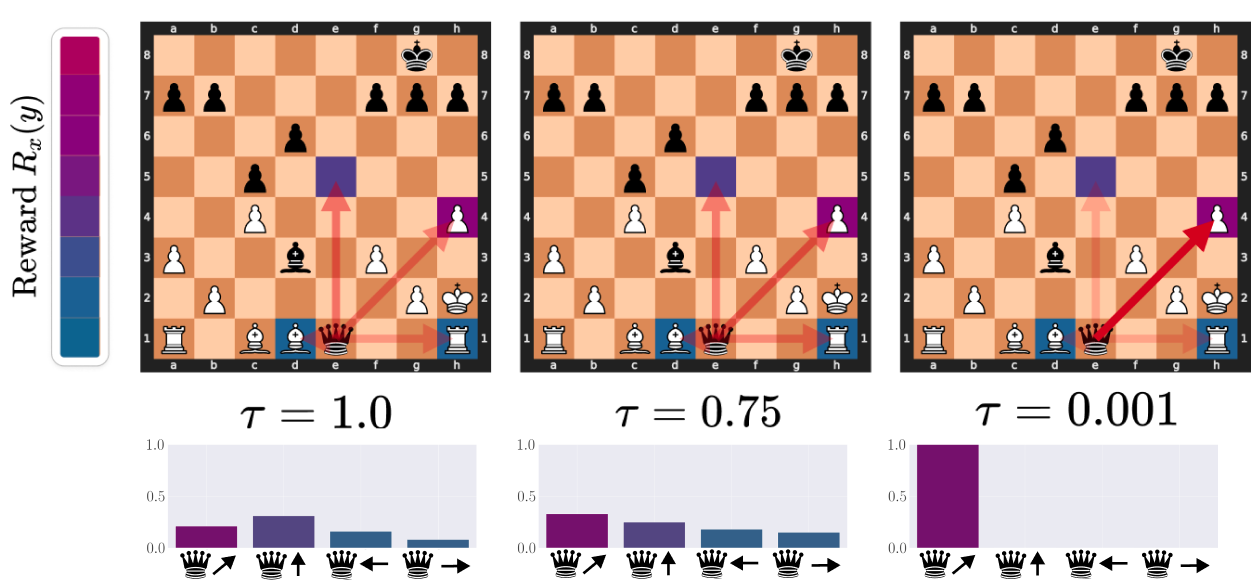
### Visual Description
# Technical Document Extraction: Chess Reward and Policy Visualization
This document analyzes a technical visualization consisting of three panels illustrating the relationship between a reward function, a temperature parameter ($\tau$), and the resulting probability distribution (policy) for a chess engine's move selection.
## 1. Global Components
### 1.1 Legend: Reward Scale
* **Location:** Far left vertical bar.
* **Label:** $\text{Reward } R_x(y)$
* **Description:** A vertical color gradient used as a heatmap for the chessboards.
* **Top (High Reward):** Bright Magenta/Purple.
* **Middle:** Deep Purple/Indigo.
* **Bottom (Low Reward):** Dark Teal/Blue.
### 1.2 Chessboard State (Common to all panels)
The image displays a mid-game chess position.
* **White Pieces:** King (h2), Rook (a1, h1), Bishop (c1, d1), Pawns (a3, b2, c4, f3, g2, h4).
* **Black Pieces:** King (g8), Queen (e1), Bishop (d3), Pawns (a7, b7, d6, c5, f7, g7, h7).
* **Active Piece:** The Black Queen on **e1** is the focus of the analysis.
* **Potential Moves Highlighted:**
1. **Diagonal Up-Right:** To h4 (Capturing White Pawn).
2. **Vertical Up:** To e5.
3. **Horizontal Left:** To d1 (Capturing White Bishop).
4. **Horizontal Right:** To h1 (Capturing White Rook).
---
## 2. Comparative Analysis by Temperature ($\tau$)
The image is divided into three columns, each representing a different value for the temperature parameter $\tau$.
### 2.1 Column 1: High Temperature ($\tau = 1.0$)
* **Chessboard Visualization:**
* The squares e5, h4, d1, and h1 are highlighted with semi-transparent colors.
* The colors are relatively muted (blues and purples), indicating a flattened reward distribution.
* Red arrows point from the Queen at e1 to these four squares with equal visual weight.
* **Bar Chart (Policy Distribution):**
* **Y-axis:** Probability (0.0 to 1.0).
* **X-axis Labels (Icons):** Queen moving Diagonal Up-Right, Vertical Up, Horizontal Left, Horizontal Right.
* **Data Points:**
* Diagonal Up-Right: ~0.22 (Magenta)
* Vertical Up: ~0.32 (Purple) - **Highest in this set**
* Horizontal Left: ~0.18 (Blue)
* Horizontal Right: ~0.08 (Dark Blue)
* **Trend:** The distribution is "soft" or "noisy." While one move is preferred, the probabilities are spread across all options.
### 2.2 Column 2: Medium Temperature ($\tau = 0.75$)
* **Chessboard Visualization:**
* The square h4 (Diagonal Up-Right) becomes a brighter magenta.
* The square e5 (Vertical Up) becomes a darker purple.
* The arrows to h4 and e5 are more prominent than the horizontal arrows.
* **Bar Chart (Policy Distribution):**
* **Data Points:**
* Diagonal Up-Right: ~0.35 (Magenta) - **Now the highest**
* Vertical Up: ~0.25 (Purple)
* Horizontal Left: ~0.18 (Blue)
* Horizontal Right: ~0.15 (Dark Blue)
* **Trend:** The distribution is beginning to peak. The highest reward move (Diagonal Up-Right) is gaining probability mass at the expense of the others.
### 2.3 Column 3: Low Temperature ($\tau = 0.001$)
* **Chessboard Visualization:**
* The square h4 is bright magenta.
* A single, thick, solid red arrow points exclusively to h4.
* Other target squares (e5, d1, h1) have very faint or no highlighting.
* **Bar Chart (Policy Distribution):**
* **Data Points:**
* Diagonal Up-Right: 1.0 (Magenta)
* Vertical Up: ~0.0
* Horizontal Left: ~0.0
* Horizontal Right: ~0.0
* **Trend:** This represents a "greedy" or "winner-take-all" selection. The move with the highest reward (Diagonal Up-Right) captures 100% of the probability distribution.
---
## 3. Summary of Data Trends
| Move Direction | Reward Color | Trend as $\tau \to 0$ | Final Probability |
| :--- | :--- | :--- | :--- |
| **Diagonal Up-Right (h4)** | Magenta (High) | Increases sharply | 1.0 |
| **Vertical Up (e5)** | Purple (Med-High) | Decreases to zero | 0.0 |
| **Horizontal Left (d1)** | Blue (Med-Low) | Decreases to zero | 0.0 |
| **Horizontal Right (h1)** | Dark Blue (Low) | Decreases to zero | 0.0 |
**Technical Conclusion:** The visualization demonstrates the effect of the **Softmax Temperature** on a policy. As $\tau$ decreases, the model transitions from a stochastic exploration of moves (where even lower-reward moves have a chance of selection) to a deterministic exploitation of the single highest-reward move.
</details>
Figure 9: Another example where denoising helps avoid errors. Moving the queen to either d1 or h1 takes a bishop or rook, respectively, but loses the queen in the following turn. While queen to e5 does not put the queen in immediate danger, it allows white to push the pawn on f3 to d3, where it threatens the queen and is protected by the bishop on c1. The queen then must move out of danger, losing its opportunity to take the free pawn on h4 and giving white valuable space towards the center of the board. As $\tau$ decreases, the expected reward converges to the move queen to d4, taking the pawn and checking the black king.
<details>
<summary>extracted/5922169/denoising_viz_3.png Details</summary>
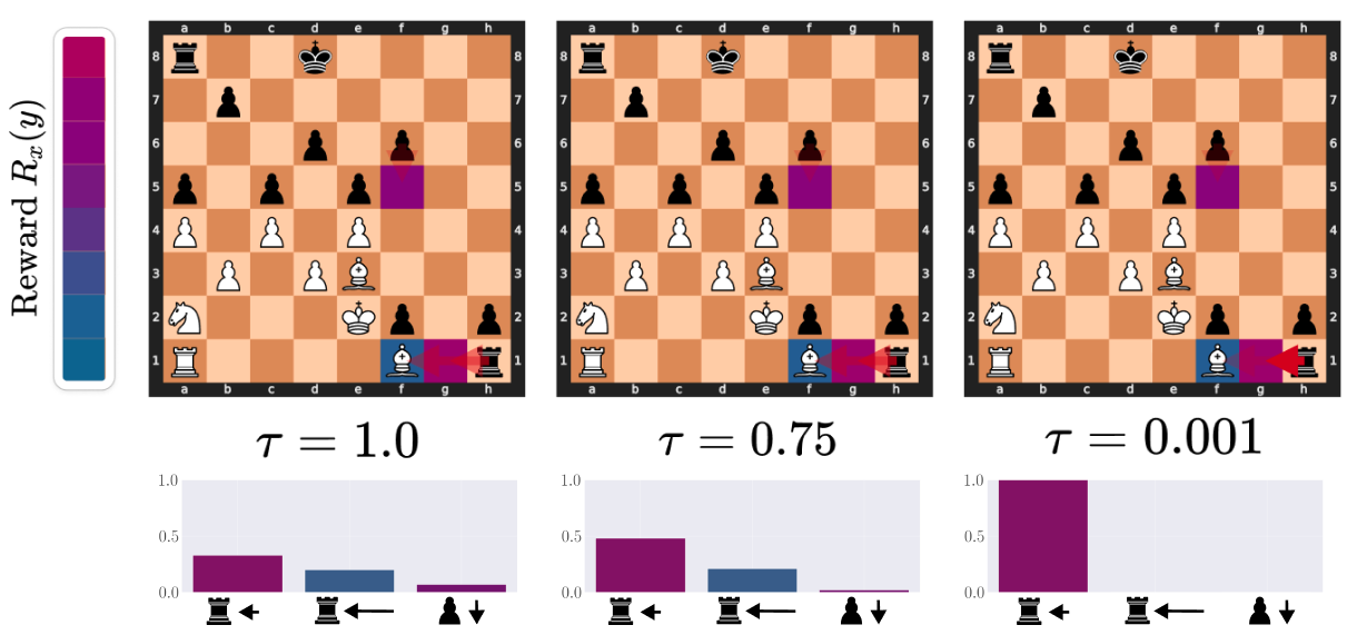
### Visual Description
# Technical Document Extraction: Chess Reward Visualization Analysis
This document provides a comprehensive technical extraction of the provided image, which illustrates the relationship between a reward function $R_x(y)$, a temperature parameter $\tau$, and the resulting probability distribution of chess moves.
## 1. Component Isolation
The image is organized into three vertical columns, each representing a different state of the temperature parameter $\tau$. Each column contains:
* **Top:** A chess board visualization with heatmaps and move arrows.
* **Middle:** A mathematical label for the temperature parameter $\tau$.
* **Bottom:** A bar chart showing the probability distribution of specific moves.
* **Left Margin:** A vertical color scale legend.
---
## 2. Legend and Scale Extraction
**Location:** Left margin $[x \approx 0, y \approx 0.3]$
* **Label:** "Reward $R_x(y)$" (Vertical orientation).
* **Type:** Discrete color gradient scale.
* **Color Mapping:**
* **Top (High Reward):** Deep Magenta/Purple.
* **Middle:** Indigo/Violet.
* **Bottom (Low Reward):** Dark Teal/Blue.
---
## 3. Main Data Analysis (By Column)
### Column 1: High Temperature ($\tau = 1.0$)
**Chess Board State:**
* **Position:** White King on e2, White Bishop on e3 and f1, White Knight on a2, White Rook on a1. Black King on d8, Black Rook on a8 and h1, Black Pawns on b7, d6, f6, a5, c5, e5, f2, h2.
* **Visual Overlays:**
* A magenta heatmap square is located at **f5**.
* A blue heatmap square is located at **f1**.
* A magenta heatmap square is located at **g1**.
* Red arrows indicate potential moves: Black Rook from h1 to g1, Black Rook from h1 to f1, and Black Pawn from f2 to f1.
* **Trend:** At $\tau = 1.0$, the probability distribution is relatively flat (high entropy), showing a spread across multiple moves.
**Bar Chart Data:**
* **Y-axis:** Probability (Scale 0.0 to 1.0).
* **X-axis Categories (Moves):**
1. **Rook to g1 (Short arrow):** ~0.33 probability (Magenta bar).
2. **Rook to f1 (Long arrow):** ~0.20 probability (Blue bar).
3. **Pawn to f1 (Down arrow):** ~0.08 probability (Magenta bar).
---
### Column 2: Medium Temperature ($\tau = 0.75$)
**Chess Board State:**
* The board configuration and overlays remain identical to the first column.
* **Trend:** As $\tau$ decreases, the distribution begins to "sharpen," favoring the highest reward move more significantly.
**Bar Chart Data:**
* **Y-axis:** Probability (Scale 0.0 to 1.0).
* **X-axis Categories (Moves):**
1. **Rook to g1:** ~0.48 probability (Magenta bar).
2. **Rook to f1:** ~0.20 probability (Blue bar).
3. **Pawn to f1:** ~0.02 probability (Magenta bar).
---
### Column 3: Low Temperature ($\tau = 0.001$)
**Chess Board State:**
* The board configuration and overlays remain identical.
* **Trend:** At a very low $\tau$, the distribution becomes "greedy." The move with the highest reward captures nearly 100% of the probability mass.
**Bar Chart Data:**
* **Y-axis:** Probability (Scale 0.0 to 1.0).
* **X-axis Categories (Moves):**
1. **Rook to g1:** ~1.0 probability (Magenta bar).
2. **Rook to f1:** ~0.0 probability (Blue bar - negligible).
3. **Pawn to f1:** ~0.0 probability (Magenta bar - negligible).
---
## 4. Summary of Findings
| Parameter | Move 1 (Rook $\leftarrow$) | Move 2 (Rook $\longleftarrow$) | Move 3 (Pawn $\downarrow$) | Distribution Characteristic |
| :--- | :--- | :--- | :--- | :--- |
| **$\tau = 1.0$** | ~0.33 | ~0.20 | ~0.08 | High Entropy / Exploratory |
| **$\tau = 0.75$** | ~0.48 | ~0.20 | ~0.02 | Moderate Focus |
| **$\tau = 0.001$** | ~1.00 | ~0.00 | ~0.00 | Deterministic / Greedy |
**Technical Conclusion:**
The image demonstrates the effect of the temperature parameter $\tau$ on a Softmax-style distribution over chess moves based on a reward function $R_x(y)$. Higher temperatures result in more uniform move selection, while lower temperatures collapse the probability onto the move with the highest perceived reward (indicated by the magenta color in the heatmap).
</details>
Figure 10: In this setup, a higher temperature shows two plausible moves for the black rook: g1 or f1. As the temperature decreases, the expected reward converges to g1. If the black rook were to move to f1, the white rook would take the black rook, blocking the black pawn on f2 from promoting and protecting the promotion square from the h2 pawn. If the rook were to move to g1, on the other hand, it would open the promotion square from the h2 pawn without being at any immediate risk. If white responded by moving its bishop to g2, protecting the promotion squares from both of the advanced black pawns, black could respond by taking the rook on a1, gaining significant material.
Appendix C Intuition of low temperature sampling inducing transcendence
To build intuition for the primary mechanism of transcendence that we explore in this paper, we give the following toy progression of distributions in order to clearly illustrate how low-temperature sampling can induce transcendence through majority voting. Here, the middle purple action represent the correct, high-reward output, whilst the left and right actions are low-reward bad outputs. We plot the probability of each output as a label on the x axis.
<details>
<summary>extracted/5922169/intuition1.png Details</summary>
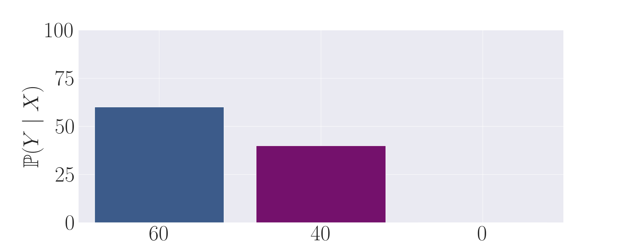
### Visual Description
# Technical Document Extraction: Probability Distribution Bar Chart
## 1. Image Classification and Overview
This image is a **bar chart** representing a discrete probability distribution. It illustrates the conditional probability of a variable $Y$ given $X$, denoted as $\mathbb{P}(Y \mid X)$. The chart features three distinct categories on the x-axis with corresponding vertical bars.
## 2. Component Isolation
### Header / Title
* **Content:** None present.
### Main Chart Area (Data Visualization)
* **Background:** Light grey with a white grid. Horizontal grid lines are aligned with the y-axis major ticks. Vertical grid lines are centered behind each x-axis label.
* **Y-Axis (Vertical):**
* **Label:** $\mathbb{P}(Y \mid X)$ (Rendered in LaTeX-style serif font).
* **Scale:** Linear, ranging from 0 to 100.
* **Markers (Ticks):** 0, 25, 50, 75, 100.
* **X-Axis (Horizontal):**
* **Label:** None explicitly titled, but contains three categorical labels.
* **Categories:** "60", "40", and "0".
* **Data Series:** Three bars of different colors and heights.
### Footer / Legend
* **Content:** None present. The values are indicated by the x-axis labels and the height relative to the y-axis.
---
## 3. Data Extraction and Table Reconstruction
The following table reconstructs the data presented in the chart. Values are estimated based on their alignment with the y-axis grid lines.
| Category (X-axis Label) | Bar Color | Estimated Value ($\mathbb{P}(Y \mid X)$) | Visual Trend Description |
| :--- | :--- | :--- | :--- |
| **60** | Dark Blue / Slate | ~60 | The tallest bar; its top sits exactly on the level of the "60" mark (interpolated between 50 and 75). |
| **40** | Purple / Magenta | ~40 | The middle bar; its top sits slightly below the 50 grid line. |
| **0** | N/A | 0 | No bar is visible; the value is at the baseline. |
---
## 4. Detailed Technical Analysis
### Trend Verification
The chart shows a **decreasing trend** from left to right based on the labels provided:
1. The first category labeled **"60"** has a probability value of approximately **60%**.
2. The second category labeled **"40"** has a probability value of approximately **40%**.
3. The third category labeled **"0"** has a probability value of **0%**.
### Mathematical Observation
The sum of the values represented by the bars ($60 + 40 + 0$) equals **100**. This confirms that the y-axis represents percentages and the chart depicts a complete probability distribution where the total probability sums to 1 (or 100%).
### Spatial Grounding
* **Y-Axis Label:** Located at the far left, rotated 90 degrees counter-clockwise.
* **Y-Axis Ticks:** Located to the left of the vertical axis line.
* **X-Axis Labels:** Centered directly beneath their respective data positions.
* **Grid:** The horizontal grid lines occur at intervals of 25 units.
## 5. Language Declaration
The text in this image is entirely in **English** (using standard Arabic numerals and mathematical notation $\mathbb{P}(Y \mid X)$).
</details>
Figure 11: The first expert output distribution. Although it puts non-negligible mass on the purple, high-reward action, it still samples a low-reward action the majority of the time.
<details>
<summary>extracted/5922169/intuition2.png Details</summary>
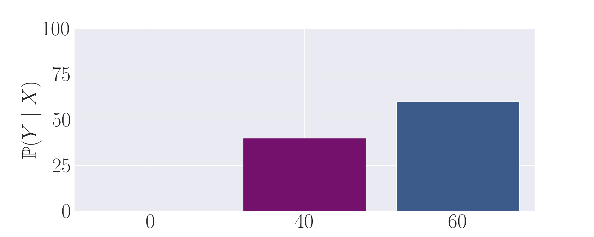
### Visual Description
# Technical Document Extraction: Probability Distribution Bar Chart
## 1. Component Isolation
* **Header:** None present.
* **Main Chart Area:** A bar chart with a light gray grid background, containing three distinct categories on the x-axis and a numerical scale on the y-axis.
* **Footer:** None present.
## 2. Axis and Label Extraction
* **Y-Axis Title:** $\mathbb{P}(Y \mid X)$ (Mathematical notation for the conditional probability of $Y$ given $X$).
* **Y-Axis Markers:** 0, 25, 50, 75, 100.
* **X-Axis Labels:** 0, 40, 60.
* **Legend:** No explicit legend is provided; however, the bars are color-coded (Purple and Blue).
## 3. Data Table Reconstruction
The chart represents the probability values for three specific instances of $X$.
| X-Axis Category | Bar Color | Estimated Y-Value ($\mathbb{P}(Y \mid X)$) | Visual Trend |
| :--- | :--- | :--- | :--- |
| **0** | N/A | 0 | No bar visible; value is at the baseline. |
| **40** | Purple | 40 | Bar rises to the level of the 40 mark (interpolated between 25 and 50). |
| **60** | Blue | 60 | Bar rises to the level of the 60 mark (interpolated between 50 and 75). |
## 4. Detailed Analysis and Trends
* **Trend Verification:** The data shows a positive correlation between the value of the X-axis label and the resulting probability $\mathbb{P}(Y \mid X)$. As the label increases from 0 to 40 to 60, the height of the bars increases accordingly.
* **Visual Encoding:**
* The category **0** has a probability of 0.
* The category **40** is represented by a solid **purple** bar. Its height aligns precisely with the numerical value of its label (40) on the y-axis scale.
* The category **60** is represented by a solid **blue** bar. Its height aligns precisely with the numerical value of its label (60) on the y-axis scale.
* **Mathematical Implication:** The chart suggests a direct identity mapping or a strong linear relationship where $\mathbb{P}(Y \mid X) = X$ for the data points shown, expressed as a percentage or a value out of 100.
## 5. Spatial Grounding
* **Origin [0,0]:** Located at the bottom left of the grid.
* **Purple Bar:** Centered over the "40" tick mark on the x-axis.
* **Blue Bar:** Centered over the "60" tick mark on the x-axis.
* **Grid Lines:** Horizontal white grid lines are placed at intervals of 25 units (0, 25, 50, 75, 100).
</details>
Figure 12: The second expert output distribution. Symmetric to to the first expert, it also puts non-negligible mass on the purple, high-reward action. However, it samples a low-reward action the majority of the time on the right.
<details>
<summary>extracted/5922169/intuition3.png Details</summary>
### Visual Description
# Technical Document Extraction: Probability Distribution Bar Chart
## 1. Component Isolation
* **Header:** None present.
* **Main Chart Area:** A bar chart with three distinct bars plotted against a light gray grid background.
* **Y-Axis (Left):** Vertical axis representing a probability or percentage scale.
* **X-Axis (Bottom):** Horizontal axis containing numerical labels for each bar.
## 2. Axis and Label Extraction
* **Y-Axis Title:** $\mathbb{P}(Y \mid X)$ (Mathematical notation for the conditional probability of Y given X).
* **Y-Axis Markers:** 0, 25, 50, 75, 100.
* **X-Axis Labels:** 30, 40, 30 (Note: These labels correspond to the values/heights of the bars).
## 3. Data Table Reconstruction
The chart visualizes three categorical data points. The height of each bar corresponds exactly to the numerical label placed directly beneath it on the x-axis.
| Bar Position | Color | Label (Value) | Estimated Y-Axis Height |
| :--- | :--- | :--- | :--- |
| Left | Dark Blue/Slate | 30 | 30 |
| Center | Purple/Magenta | 40 | 40 |
| Right | Dark Blue/Slate | 30 | 30 |
## 4. Trend and Visual Analysis
* **Symmetry:** The chart displays a symmetrical "bell-like" distribution pattern. The outer two bars are identical in height and color, while the center bar is taller and a different color.
* **Color Coding:**
* The bars representing the value **30** are colored in a dark blue/slate shade.
* The bar representing the value **40** is colored in a deep purple/magenta shade.
* **Visual Trend:** The data follows a "Low-High-Low" sequence. Starting from the left, the value rises from 30 to 40 (a 33.3% increase) and then returns to 30.
* **Total Sum:** The sum of the values shown (30 + 40 + 30) equals **100**, which is consistent with the Y-axis scale representing a full probability distribution (100%).
## 5. Technical Description
This image is a bar chart representing a discrete conditional probability distribution $\mathbb{P}(Y \mid X)$. The vertical axis ranges from 0 to 100. The chart contains three bars. The first and third bars have a value of 30 and are colored dark blue. The middle bar has a value of 40 and is colored purple. The total area/value of the bars sums to 100, indicating these are likely percentage-based probabilities for three possible outcomes of $Y$ given a specific $X$. The background features a light gray grid with white grid lines aligned with the Y-axis markers at intervals of 25.
</details>
Figure 13: By taking the average of the first and second expert, we observe that this distribution now puts the majority of mass onto the correct action.
<details>
<summary>extracted/5922169/intuition4.png Details</summary>
### Visual Description
# Technical Document Extraction: Probability Distribution Chart
## 1. Image Overview
This image is a bar chart representing a conditional probability distribution. It features three distinct bars against a light gray grid background. The chart uses color coding to differentiate between high and low probability values.
## 2. Component Isolation
### Header/Title
* No explicit title text is present in the image.
### Main Chart Area (Data Visualization)
* **Type:** Vertical Bar Chart.
* **Y-Axis (Vertical):**
* **Label:** $\mathbb{P}(Y \mid X)$ (Mathematical notation for the conditional probability of $Y$ given $X$).
* **Scale Markers:** 0, 25, 50, 75, 100.
* **X-Axis (Horizontal):**
* **Categories/Labels:** "5", "90", "5".
* **Grid:** Horizontal white grid lines are placed at the 25, 50, 75, and 100 markers.
### Footer/Legend
* There is no separate legend box. The data values are labeled directly beneath each bar on the x-axis.
## 3. Data Extraction and Trend Verification
### Trend Analysis
The chart shows a highly peaked distribution (leptokurtic). The central category holds the vast majority of the probability mass, while the two flanking categories represent minor, equal portions of the distribution.
### Data Table Reconstruction
Based on the visual alignment with the y-axis markers and the labels provided on the x-axis:
| X-Axis Category (Label) | Color | Estimated Y-Value ($\mathbb{P}(Y \mid X)$) |
| :--- | :--- | :--- |
| 5 | Dark Blue | 5 |
| 90 | Deep Purple/Magenta | 90 |
| 5 | Dark Blue | 5 |
### Spatial Grounding & Logic Check
* **Left Bar:** Labeled "5". The color is dark blue. Visually, the top of the bar sits significantly below the "25" grid line, consistent with a value of 5.
* **Center Bar:** Labeled "90". The color is deep purple. Visually, the top of the bar sits exactly halfway between the "75" and "100" grid lines (which would be 87.5), but slightly higher, confirming the "90" label.
* **Right Bar:** Labeled "5". The color is dark blue. Visually identical in height to the first bar, confirming the value of 5.
* **Summation Check:** $5 + 90 + 5 = 100$. This confirms the chart represents a full probability distribution where the total sum equals 100%.
## 4. Textual Transcription
* **Y-Axis Label:** `P(Y | X)` (rendered in LaTeX style as `\mathbb{P}(Y \mid X)`)
* **Y-Axis Markers:** `0`, `25`, `50`, `75`, `100`
* **X-Axis Labels:** `5`, `90`, `5`
</details>
Figure 14: Finally, by setting temperature $\tau$ to be $<1$ , more weight is shifted towards the high probability action, leading to a gain in the expected reward.
Appendix D Further Related Work
D.1 Label Disagreement
Label disagreement in training data, in particular, can improve models in practice. Xie et al. [36] empirically show that adding random noise to teacher-generated labels can improve a student model. Uma et al. [33] even survey the literature on human interannotator disagreement and find a trend of improvements when models are trained on the full set of disagreeing labels rather than on majority vote labels or only on data where labelers agree. Our theoretical claims build on these findings by making the point that the learner can even improve on these original diverse labelers.
D.2 Offline Reinforcement Learning
Although most Offline Reinforcement Learning algorithms train on an RL objective, perhaps most similar to our work is Decision Transformer [4] and Trajectory Transformer [8]: prior models trained on just the sequence prediction of trajectories. Most notably, Decision Transformer also finds an alternative form of transcendence than the one explored in this paper: by conditioning the trained transformer by the performance of the trajectory, at inference time they can then prompt the model to perform better than the best trajectory seen during training. This remains another promising direction to explore transcendence under.
Interestingly, an analogue to low-temperature sampling also has been noticed and exploited by Reinforcement Learning practitioners in the context of off-policy learning, where a different exploration policy $\pi_{E}$ is used than the final learned target policy $\pi_{T}$ . Oftentimes $\pi_{T}$ will just be set to a greedy version of $\pi_{E}$ [21], such as choosing $\pi_{T}$ to take the $\operatorname*{arg\,max}$ action of $\pi_{E}$ , which we note is directly equivalent to setting temperature to 0.
Appendix E Training Details
We give a full list of the hyperparameters we used for training here. Note that we largely follow the same hyperparameter set as [37], but lower the batch size to $125K$ as we found training to still be stable ta this level. We also release our code openly to support further research into transcendence, which was built off the wonderful work done by Karvonen [12] and Karpathy [11].
| ChessFormer | Optimizer Activation Function Mini-batch size | AdamW [13] ReLU 125K tokens |
| --- | --- | --- |
| Gradient Accumulation Steps | 1 | |
| Transformer num. layers | 16 | |
| Transformer num. heads | 8 | |
| Transformer embedding dim. | 512 | |
| Dropout | 0.0 | |
| Learning Rate | 3e-4 | |
| Number of gradient steps | 100K | |
| Weight Decay | 0.1 | |
| Critic hidden layers | 3 | |
| Adam $\beta_{1}$ | 0.90 | |
| Adam $\beta_{2}$ | 0.95 | |
| Gradient Clip | 1.0 | |
| Cosine Learning Rate | True | |
| Warmup Iterations | 2000 | |
| Minimum Learning Rate | 3e-5 | |
| Learning Rate Deacy Iterations | 400K | |
| Tensor datatype | bfloat16 | |
Table 2: Hyperparameters for our ChessFormer model.
Appendix F Compute Resources
We train all of our models on the Nvidia H100 80GB GPU. To train one of our models takes around 6 to 12 hours.
Appendix G Full t-SNE
We visualize the full t-SNE here, coloring by the reward of the game. We see that the model has learned some representation of the reward, with high absolute reward states being more likely to be near each other in the latent space. This also points towards evidence that the model has learned some sort equivariant representation of the player identity, as the region of symmetric high reward states indicate. Note that reward is not directly given to the model during training.
{adjustwidth}
-0.1-0.1
<details>
<summary>x4.png Details</summary>
### Visual Description
# Technical Document Extraction: Scatter Plot Analysis
## 1. Component Isolation
* **Header Region:** Contains a partial text string in a serif font.
* **Main Chart Region:** A vertical, high-density scatter plot (likely a t-SNE or UMAP visualization) showing clusters of data points.
* **Footer Region:** Contains a single numerical axis marker.
---
## 2. Textual Information Extraction
### Header Text
* **Transcribed Text:** `rd States`
* **Contextual Inference:** This appears to be the suffix of a title, likely "Standard States" or "Ground States," cut off by the image cropping.
### Footer/Axis Labels
* **Numerical Marker:** `0`
* **Placement:** Centered at the bottom of the horizontal axis.
---
## 3. Data Visualization Analysis (Main Chart)
### Type and Structure
The image is a **high-dimensional dimensionality reduction plot** (scatter plot). It visualizes thousands of individual data points projected onto a 2D plane to show clustering and relationships.
### Color Coding (Data Series)
There is no explicit legend present in the cropped image, but three distinct color populations are visible throughout the clusters:
1. **Purple/Violet:** The most dominant color, forming the "background" or majority of most clusters.
2. **Red/Crimson:** Concentrated in specific sub-regions of clusters, indicating a specific state or category.
3. **Teal/Blue-Green:** Sparsely distributed, often appearing on the periphery of clusters or mixed within purple regions.
### Spatial Distribution and Trends
The data is organized into several distinct morphological structures:
* **Top Region:** Features a large, rectangular-ish cluster at the top right and several smaller, elongated "island" clusters.
* **Middle Region:** Contains highly branched, dendritic structures. These "starburst" patterns suggest a central state with multiple divergent paths or transitions. There is a very high-density circular "core" in the lower-middle section dominated by red and purple points.
* **Bottom Region:** Features more isolated, dense "blob" clusters. The very bottom of the plot shows a few scattered, individual outlier points.
### Trend Verification
* **Clustering Trend:** The data does not follow a linear or functional trend (like a line graph). Instead, it follows a **topological trend** where points are grouped by similarity.
* **Color Mixing:** In the central high-density region, there is a significant overlap between Red and Purple points, suggesting these two categories share similar spatial/mathematical characteristics in this projection.
* **Isolation:** The Teal points appear more frequently in the smaller, isolated clusters at the top and bottom-left, suggesting they represent a more distinct or rare state compared to the Purple/Red majority.
---
## 4. Summary of Facts
* **Data Type:** Categorical scatter plot (3 categories).
* **Language:** English (Latin script).
* **Key Feature:** Complex, branched clustering indicating non-linear relationships between data points.
* **Axis:** Horizontal axis is marked with `0` at the center; vertical axis has no visible markers.
</details>
We visualize the same t-SNE, but this time coloring by game length rather than reward. We see that games with high reward tend to be longer, which makes logical sense as the result of the game will tend to be clearer as the game proogresses.
{adjustwidth}
-0.1-0.1
<details>
<summary>x5.png Details</summary>

### Visual Description
# Technical Document Extraction: Scatter Plot Analysis
## 1. Document Overview
This image is a high-resolution, vertically oriented scatter plot, likely representing a dimensionality reduction visualization (such as t-SNE or UMAP) used in bioinformatics or machine learning to show clusters of data points.
## 2. Component Isolation
### Header Region
- **Text Fragment:** "States C"
- **Description:** A partial title is visible at the top, cut off by the image frame. It is rendered in a serif font. A horizontal black line separates the header text from the main chart area.
### Main Chart Region (Data Visualization)
- **Type:** Scatter Plot / Point Cloud.
- **Data Points:** Thousands of individual micro-dots.
- **Color Gradient:** The points follow a color scale ranging from **Teal/Dark Blue** to **Bright Purple/Magenta**.
- **Spatial Distribution:**
- **Central Density:** There is a high concentration of purple points near the vertical center of the image, suggesting a core state or a high-density region in the original high-dimensional space.
- **Peripheral Clusters:** Numerous smaller, more isolated clusters are scattered throughout the top and bottom of the frame. These are predominantly teal/blue, with occasional purple highlights.
- **Morphology:** Some clusters appear dendritic (branch-like), while others are more globular or elongated.
### Footer Region (Axis)
- **Axis Marker:** A single numerical label **"0"** is centered at the bottom.
- **Axis Line:** A solid black horizontal line serves as the X-axis.
- **Tick Mark:** A small vertical tick mark is positioned directly above the "0".
## 3. Trend and Data Verification
- **Color-Spatial Correlation:** There is a clear gradient trend where the central-most clusters (relative to the vertical axis) exhibit the highest concentration of purple/magenta points. As the clusters move toward the top or bottom extremes of the image, the color shifts toward teal/dark blue.
- **Density Trend:** The center of the plot appears to have the highest point density, with points becoming more sparse and clusters becoming more discrete toward the edges.
## 4. Extracted Textual Information
| Category | Content |
| :--- | :--- |
| **Partial Title** | States C |
| **X-Axis Label** | 0 |
| **Language** | English |
## 5. Technical Summary
The image depicts a complex data manifold. The presence of the word "States" and the "0" axis marker suggests this may be a visualization of latent states in a dynamical system or cell states in a single-cell sequencing dataset. The color gradient likely represents a third dimension or a specific metadata value (e.g., time, expression level, or probability density) mapped onto the 2D coordinates.
</details>