2406.13803v1

# Semantic Structure-Mapping in LLM and Human Analogical Reasoning **Authors**: Sam Musker, Alex Duchnowski, Raphaël Millière, Ellie Pavlick ## Abstract Analogical reasoning is considered core to human learning and cognition. Recent studies have compared the analogical reasoning abilities of human subjects and Large Language Models (LLMs) on abstract symbol manipulation tasks, such as letter string analogies. However, these studies largely neglect analogical reasoning over semantically meaningful symbols, such as natural language words. This ability to draw analogies that link language to non-linguistic domains, which we term semantic structure-mapping, is thought to play a crucial role in language acquisition and broader cognitive development. We test human subjects and LLMs on analogical reasoning tasks that require the transfer of semantic structure and content from one domain to another. Advanced LLMs match human performance across many task variations. However, humans and LLMs respond differently to certain task variations and semantic distractors. Overall, our data suggest that LLMs are approaching human-level performance on these important cognitive tasks, but are not yet entirely human like. keywords: language models , analogies , structure-mapping journal: review. [label1]organization=Brown University,addressline=Department of Computer Science, city=Providence, postcode=02912, state=RI, country=USA [label2]organization=Macquarie University,addressline=Department of Philosophy, city=Sydney, postcode=2109, state=NSW, country=Australia ## 1 Introduction The recent advances of large language models (LLMs) have raised the question of whether LLMs can serve as useful cognitive models in the study of various aspects of human learning, cognition, and behavior [1, 2, 3]. One such recent debate has focused on whether LLMs acquire the ability to perform analogical reasoning as a by-product of their self-supervised learning objective [4, 5, 6, 7]. Analogical reasoning—the ability to align abstract structures between a source and target domain—is posited to play a central role in human learning and generalization, for example, our ability to reason efficiently in unfamiliar domains [8, 9]. Thus, the question of whether LLMs can reason analogically in a human-like way directly bears on their ability to serve as computational models of human behavior beyond just next-word prediction. Recent work has focused on the ability of advanced LLMs to match human analogical reasoning performance on tasks that involve recognition of spatial and logical transformations in matrices [4] or detecting patterns in strings of letters or numbers [7]. For example, Mitchell [7] uses analogy tasks such as abcd:abce::ijkl:?? in order to test the extent to which LLMs and humans can recognize and generalize abstract structures and operations (in this example, ordered sequences and successor functions). Such studies have produced mixed results, with evidence suggesting that advanced LLMs achieve the same performance and even produce similar error patterns to those observed in humans [4, 6], but with doubts remaining about the robustness of LLMs’ abilities, particularly with respect to increasingly abstract and challenging domains [10]. Previous work has focused almost exclusively on analogies using abstract and arbitrary symbols, where structures are derived from symbols’ spatial positions in the text prompt, but the symbols themselves are unimportant. This leaves out questions about reasoning analogically over semantically meaningful symbols, such as words in natural language. This type of analogical reasoning, which we call semantic structure-mapping, requires mapping between semantic structure in one domain (e.g., the relationship between a dog and a puppy, or that a dog has four legs) and non-semantic (arbitrary) structure in the other domain (e.g., spatial position in the text prompt). This type of mapping is thought to play a crucial role in human cognition and development, such as in the language-analogical reasoning feedback loop proposed by Structure-Mapping Theory (SMT) [11]. Moreover, if LLMs are to provide insight into how humans perform certain cognitive functions, it will likely involve the role of distributional semantic learning [12, 13, 14] in the acquisition or representation of those functions. Therefore, we focus on investigating how humans and LLMs compare in tasks requiring semantic structure-mapping and assessing whether patterns differ from those observed on tasks involving only arbitrary symbols. We design two experiments, focused respectively on the mapping of semantic structure (i.e., semantic relationships between symbols, such as relating the symbol dog to the symbol puppy) and semantic content (i.e., information attached to a symbol such as the knowledge that a dog has four legs). In each experiment, the subject (human or LLM) is presented with a set of left-hand terms (the source domain) and a corresponding set of right-hand terms (the target domain), with the final right-hand term omitted. The subject is asked to fill in this blank. An exact copy of our prompt and an example question is shown in Figure 1. We design multiple variants of such questions designed to probe structure-mapping that involves semantic structure and semantic content, respectively. We additionally design a series of control and distractor conditions—e.g., interleaving informative mappings (square => C C C) with uninformative ones (lime => X X X) in order to expose differences in the underlying mechanism. Overall, the most advanced LLMs we tested match human performance across our primary conditions, even producing human-like error patterns. However, significant differences emerge in several control settings. Even the most advanced LLMs show more sensitivity than humans to information presentation order and struggle to ignore irrelevant semantic information that humans readily dismiss. Thus, our results contribute to the ongoing debate about analogical reasoning, corroborating both work arguing for impressive LLM performance [4, 15] and work highlighting important mechanistic differences between humans and LLMs [10, 16]. Code and data are available at https://github.com/AnonymousReview123/Semantic_Structure_Mapping_Anon. By presenting data on the unique role of semantic structure and content in analogical reasoning, we suggest differences remain in how LLMs and humans represent and map semantic structure, although this gap may be closing as models increase in size and incorporate more diverse training signals. We argue that this has important implications for studying cognitive development and the role of LLMs in this research going forward. ## 2 Methods ### 2.1 Experiment Details #### 2.1.1 Semantic Structure Each subject was presented with a quiz, which is a sequence of four such questions generated using four sets of base domains and four sets of target domains selected such that a participant sees each base and target domain exactly once. Eight variants of the task were devised to investigate the influence of task variations as described above. Questions are introduced with the prompt “We are conducting an experiment on general reasoning abilities. Below we will show you various words and drawings of each, after which you will need to complete the last drawing. Respond as concisely as possible with only the last drawing.” We use the term “drawings” to describe the elements in the target domain because it loosely encapsulates the idea of mapping between the source and target domains. In a similar way to how drawings serve as partial structurally isomorphic representations that depict a subject with varying degrees of abstraction [17], the elements in our target domains establish a space of relations that are isomorphic to those in the source domain. In some cases the term “drawing” is straightforwardly applicable, as when the capitalization of characters corresponds to the term for a mature animal. In other cases the use is strained, as when capitalization instead corresponds to a shape being symmetrical. The transparently liberal use of the term “drawing” is used to prime subjects to reason creatively while attending to the correspondence between source and target domains. The prompt’s lack of reference to analogical reasoning accesses pre-theoretic responses to the extent possible. For the same purpose the experiment is introduced to human subjects and LLMs as studying “general reasoning abilities.” #### 2.1.2 Semantic Content Each condition (described in Table 4) contains two quizzes, with four questions per quiz. Unless otherwise stated, methodological details of the Semantic Content experiment match those of the Semantic Structure experiment. The four conditions are divided into those that require numeric reasoning and those that do not. Within the numeric and non-numeric conditions respectively, one condition utilizes only one dimension of variation (referred to as “single-attribute”) whereas another adds a second dimension of variation (“multi-attribute”). This allows for comparing the relative performance of human subjects and models when the task is made to require compositional reasoning over layered transformations. Questions were formatted like the following example: | horse => * * * * | | --- | | cat => * * * * | | ant => ! ! ! ! ! ! | | bee => ! ! ! ! ! ! | | chicken => ! ! | | spider => ! ! ! ! ! ! ! ! | | dog => * * * * | | human => | In this example, the number of symbols corresponds to a number-of-legs feature, and the usage of exclamation marks and asterisks corresponds to an egg-laying feature (or, alternatively, a mammal feature). The right-hand sequences of characters thereby encode properties of the entities denoted by the left-hand words. Given that humans are two-legged mammals, the correct answer here would be * *. In order to solve this task, the participant must understand both aspects of the information encoded in the right-hand terms and then construct the answer by generalizing to a new example. ### 2.2 Participants #### 2.2.1 LLMs We run our experiments on the following LLMs: GPT-3 [18], GPT-4 [19], Pythia-12B [20], Claude 2 [21], Claude 3 Opus [22], and Falcon-40B [23]. All of the above are transformer-based LLMs trained primarily on a next word prediction objective. GPT-3 consists of a 175B parameter model trained on text completion and finetuned to produce more coherent answers. The details of GPT-4 are not publicly known, but it is considered by some sources to be a mixture-of-experts (MoE) model consisting of numerous GPT-3-scale language models [24]. GPT-4, unlike GPT-3, supplements text-completion pretraining and finetuning with reinforcement learning from human feedback (RLHF) in order to better align model outputs with the expectations of a human user. The training of Claude 2 also includes RLHF, but its performance falls short of GPT-4. The more recent Claude 3 (in our case, the most advanced Opus version) is considered to approximately match GPT-4 performance in general. GPT-3 and -4 are developed by OpenAI, whereas Claude 2 and 3 are developed by Anthropic. Pythia-12B and Falcon-40B are open-weights LLMs trained on a text-completion objective and consist of 12B and 40B parameters respectively. Neither undergoes RLHF. Pythia-12B is developed by EleutherAI, and Falcon-40B is developed by the Technology Innovation Institute. #### 2.2.2 Human Subjects We also test human participants on our experiments. Reported in the main text are results obtained from 194 (mostly undergraduate) University-Name University students (132 in the Semantic Structure experiment, and 62 in the Semantic Content experiment). The split of participants between experiments approximately matches the 9:4 ratio of experiment conditions. The number of participants by condition are as follows: Defaults 18, Distracted 18, Only RHS 18, Permuted Pairs 17, Permuted Questions 17, Random Finals 15, Random Permuted Pairs 6, Randoms 8, Relational 15, Categorial 16, Multi Attribute 16, Numeric 16, Numeric Multi Attribute 14. The Relational, Categorial, Multi Attribute, Numeric, and Numeric Multi Attribute conditions each have two quizzes while the remaining conditions each have four quizzes per condition. Subjects were assigned randomly to a single quiz from one condition without the re-use of subjects. Roughly the same number of participants were assigned to each condition, with the exception of the Random and Random Permuted Pairs conditions. These were together assigned roughly the expected number of subjects for a single condition due to their similarity. The subjects were recruited through email advertisements and offered $10 in compensation. Earlier results obtained for the Semantic Structure experiment from an online sample of participants recruited through Prolific are reported in Figure 11 of the Appendix. We ensure that humans and LLMs are given comparable information in our prompting design. A given human participant sees one quiz with four questions, with questions revealed one at a time with the answer shown following each response. LLMs are prompted with the first question of a quiz, then the second question with the first question and its (correct) answer accumulating in the prompt, and so forth for the four questions in a quiz. This prompt accumulation mimics the availability in the memory of human subjects of previous answers within a quiz. ### 2.3 Statistical testing In each experiment, we are interested in the relative performance of human subjects and the best-performing models and how this depends on the particular experiment conditions. Differences between most models and human subjects are large and do not require statistical analysis, and so we focus our statistical analysis on the performance of GPT-4 relative to human subjects and Claude 3 relative to human subjects. For each experiment and pair of subjects (human subjects and GPT-4, or human subjects and Claude 3) we fit a logistic model to the data with and without interactions between the subject type and the experiment condition. In all cases, the outcome variable is the un-aggregated per-question score achieved by a subject (either a 0 or 1), and the predictor variables are experiment condition (e.g. “Defaults” or “Permuted Pairs”) and subject type (e.g. “human subjects” or “GPT-4”). We use four likelihood ratio tests to assess whether the interaction between subject type and experiment condition is significant for a given pair of subjects within a particular experiment, as motivated by Glover [25]. In all four cases the interaction is significant, and so we use simple effects analysis to investigate the direction and significance of the effect of subject type within particular conditions. For the semantic content experiment, we additionally perform a logistic simple effects analysis comparing the performance of a single subject type (human, GPT-4, or Claude 3) in compositional versus non-compositional conditions for the numeric and non-numeric cases respectively with the non-compositional condition as reference. For example, we assess the effect of the condition being Multi Attribute with Categorial as the reference condition for only the subject type Claude 3 (and likewise for the other two examined subject types). Further details are provided in Sections A.1 and A.2 of the Appendix. ## 3 Results ### 3.1 Mapping Semantic Structure We first design a set of experiments investigating the ability of LLMs and human subjects to map semantic structure in the source domain onto arbitrary, non-semantic structure in the target domain. In this set of experiments, our source domain (left-hand side) is a set of words which are assumed to possess some relational structure, and our target domain (right-hand side) is a set of strings related via non-linguistic string operations. | We are conducting an experiment on general reasoning abilities. Below we will show you various words and drawings of each, after which you will need to complete the last drawing. Respond as concisely as possible with only the last drawing. | | --- | | Question 1: | | square => C C C | | rectangle => c c c | | circle => C C | | oval => | square rectangle circle oval C C C c c c C C c c Figure 1: An example question (from the Defaults condition of the Semantic Structure experiment) with a representation of the structure-mapping solution below. The source domain is in blue and the target domain is in orange (for the provided elements) and yellow (for the inferred element). #### 3.1.1 Overall Performance Human subjects perform well overall, obtaining accuracy between 0.4 and 0.9 across the various conditions. The most advanced LLMs that we test attain accuracies in the range 0.1-0.95 across conditions. This performance range is comparable to prior work on analogical reasoning over arbitrary symbols. For example, the results of human subjects on the “zero-generalization setting” studied by both Webb et al. [4] and Mitchell et al. [10] range from 0.2-0.8 in the former study and from 0.5-1.0 in the latter study. Similarly, results for LLMs (GPT-3, GPT-3.5, and GPT-4) across those conditions range from 0.1-1.0 in the two studies. Thus, our data suggest that analogies involving semantic structure-mapping are not inherently easier or harder than those which make use of arbitrary symbols. Our Defaults condition consists of lexical items as a source domain and one of several string operation relations as a target domain. To investigate the robustness of performance metrics, we introduce three control conditions: (1) Permuted Questions, in which we present unaltered versions of the core task with varied question ordering; (2) Permuted Pairs, in which we alter the order in which the lines of the analogy are presented; and (3) Distracted, in which we interleave unrelated mappings between the lines of the target analogy. These conditions are shown in Table 1. We do not expect Permuted Questions to materially alter the task, but might see some effect of the Permuted Pairs and Distracted conditions, as they could make the relevant relations less transparent: see, for example, work on the blocking advantage in humans [26] and in LLMs [27]. | Defaults | Basic test of semantic structure-mapping | square => C C C rectangle => c c c circle => C C oval => | | --- | --- | --- | | Permuted Pairs | Like Defaults, but with row order permuted | rectangle => c c c circle => C C square => C C C oval => | | Distracted | Like Defaults, but with a distractor row added | square => C C C rectangle => c c c pillow => A P circle => C C oval => | Table 1: Defaults and control conditions used to measure ability of humans and LLMs to perform analogical reasoning tasks that involve semantic structure-mapping. The Permuted Questions condition (not shown) is identical to Defaults, but with question order permuted. 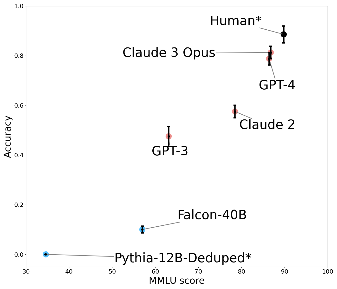Figure 2 shows the performance of humans and LLMs in the Defaults condition as a function of their performance on MMLU MMLU scores are few-shot for GPT-4 and 5-shot for other models. The reported human baseline is the estimate for human experts given by Hendrycks et al. [28]. The score for Pythia 12B could not be found and so we use the reported value for Pythia 6.9B Tulu., a widely-used language competency benchmark. Increasing MMLU score is associated with higher accuracy on the Defaults condition. Smaller models do not perform competitively (Pythia-12B obtains an accuracy of 0.0, Falcon 40B 0.1, GPT-3 0.5, and Claude 2 0.6). This steadily increasing performance is presumed to correlate with the scale of model parameters and training data [29]. We focus our remaining analysis on comparing human subjects to GPT-4 and Claude 3. In the Defaults condition, neither GPT-4 (coef=-0.7696, z=-1.659, p=0.097) nor Claude 3 (coef=-0.6131, z=-1.299, p=0.194) performs significantly worse than human subjects. <details> <summary>extracted/5679376/Images/Comparison_Default_MMLU.png Details</summary>  ### Visual Description ## Scatter Plot with Error Bars: AI Model Performance vs. Human Benchmark on MMLU ### Overview The image is a scatter plot comparing the performance of various large language models (LLMs) and a human benchmark on two metrics: "MMLU score" (x-axis) and "Accuracy" (y-axis). Each data point represents a model or human performance, accompanied by error bars indicating uncertainty. The plot demonstrates a positive correlation between MMLU score and accuracy. ### Components/Axes * **X-Axis:** Labeled "MMLU score". Scale ranges from 30 to 100, with major tick marks at 30, 40, 50, 60, 70, 80, 90, and 100. * **Y-Axis:** Labeled "Accuracy". Scale ranges from 0.0 to 1.0, with major tick marks at 0.0, 0.2, 0.4, 0.6, 0.8, and 1.0. * **Data Series & Labels:** Seven distinct data points are plotted, each labeled directly on the chart. The labels are connected to their respective points by thin gray lines. * **Pythia-12B-Deduped\*** (Blue point, bottom-left) * **Falcon-40B** (Blue point, lower-middle) * **GPT-3** (Red point, center) * **Claude 2** (Red point, upper-middle right) * **GPT-4** (Red point, upper-right) * **Claude 3 Opus** (Red point, upper-right, slightly above GPT-4) * **Human\*** (Black point, top-right) * **Error Bars:** Vertical black bars extend above and below each data point, representing the range of uncertainty or variance for the "Accuracy" metric. ### Detailed Analysis **Data Point Extraction (Approximate Values):** | Model / Entity | MMLU Score (X) | Accuracy (Y) | Error Bar Range (Accuracy) | Point Color | | :--- | :--- | :--- | :--- | :--- | | Pythia-12B-Deduped* | ~35 | ~0.00 | Very small, near zero | Blue | | Falcon-40B | ~57 | ~0.10 | ~0.08 to ~0.12 | Blue | | GPT-3 | ~62 | ~0.47 | ~0.42 to ~0.52 | Red | | Claude 2 | ~78 | ~0.57 | ~0.55 to ~0.60 | Red | | GPT-4 | ~86 | ~0.79 | ~0.77 to ~0.82 | Red | | Claude 3 Opus | ~87 | ~0.81 | ~0.79 to ~0.83 | Red | | Human* | ~90 | ~0.88 | ~0.85 to ~0.91 | Black | **Trend Verification:** * The overall visual trend is a clear upward slope from the bottom-left to the top-right. As the MMLU score increases, the Accuracy score also increases. * **Pythia-12B-Deduped*:** Positioned at the extreme bottom-left, showing near-zero accuracy with a low MMLU score. * **Falcon-40B:** Shows a modest increase in both metrics compared to Pythia. * **GPT-3:** Represents a significant jump in accuracy from the previous models. * **Claude 2:** Continues the upward trend, positioned higher and to the right of GPT-3. * **GPT-4 & Claude 3 Opus:** Clustered closely together in the upper-right quadrant, indicating high performance on both metrics. Claude 3 Opus is marginally higher in accuracy and MMLU score. * **Human*:** Positioned as the top-right outlier, achieving the highest scores on both axes. ### Key Observations 1. **Performance Hierarchy:** The plot establishes a clear performance hierarchy: Human* > Claude 3 Opus ≈ GPT-4 > Claude 2 > GPT-3 > Falcon-40B > Pythia-12B-Deduped*. 2. **Model Generations:** The data visually groups models by generation or capability tier. The latest models (Claude 3 Opus, GPT-4) are clustered near human performance, while older models (GPT-3, Falcon-40B) are significantly lower. 3. **Error Bar Variance:** The length of the error bars varies. GPT-3 has a notably wider error bar in accuracy compared to others like Claude 2 or GPT-4, suggesting greater uncertainty or variance in its performance on this specific evaluation. 4. **Color Coding:** Models are color-coded. The two lowest-performing models (Pythia, Falcon) are blue. The mid-to-high performing AI models (GPT-3, Claude 2, GPT-4, Claude 3 Opus) are red. The human benchmark is uniquely black. ### Interpretation This chart illustrates the rapid advancement of AI language models on the MMLU (Massive Multitask Language Understanding) benchmark, a standard test of broad knowledge and problem-solving. The strong positive correlation between MMLU score and Accuracy suggests that performance on this benchmark is a reliable predictor of general accuracy in the evaluated tasks. The key takeaway is the closing gap between top-tier AI models and human performance. Claude 3 Opus and GPT-4 operate at approximately 90% of the human accuracy level shown here, marking a significant milestone. The asterisk (*) on "Human*" and "Pythia-12B-Deduped*" likely denotes a specific condition or footnote not visible in the image (e.g., "Human" may represent an average of expert performance, and "Deduped" refers to a data deduplication process for the Pythia model). The plot serves as a snapshot of the competitive landscape in AI development as of the data's collection, highlighting both the achievements of leading models and the remaining margin to reach and surpass human-level performance on this comprehensive benchmark. </details> Figure 2: Human and LLM accuracy in the Defaults condition, relative to performance on the MMLU benchmark. Models in blue are not instruction-tuned while models in orange are. Error bars show standard errors. 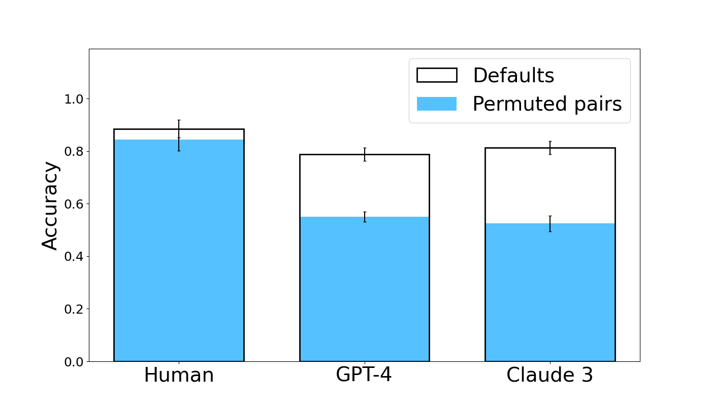Figure 3 compares humans to high-performing LLMs in the Defaults and Permuted Pairs conditions. LLM performance drops in the Permuted Pairs condition, while humans seem equally able to infer the mapping regardless of word presentation order. This effect is significant for both Claude 3 (coef = -1.7802, z = -4.217, p < 0.001) and GPT-4 (coef = -1.6796, z = -3.975, p < 0.001). This suggests that, while the overall performance is comparable, there are likely meaningful mechanistic differences in how the analogy is processed in humans versus LLMs. The remaining control conditions and data for all tested models are shown in Figure 15 of the Appendix . In these conditions, we find that humans and models are roughly equally affected. For example, accuracy in the Distracted condition drops by approximately 0.25 for all three subject types. <details> <summary>extracted/5679376/Images/fig3_new.png Details</summary>  ### Visual Description ## Bar Chart: Accuracy Comparison of Human and AI Models Under Default and Permuted Pair Conditions ### Overview The image is a grouped bar chart comparing the accuracy of three entities—Human, GPT-4, and Claude 3—under two experimental conditions: "Defaults" and "Permuted pairs." The chart visually demonstrates a performance gap between the two conditions for each entity, with a notably larger drop for the AI models. ### Components/Axes * **Chart Type:** Grouped bar chart with error bars. * **Y-Axis:** Labeled "Accuracy." The scale runs from 0.0 to 1.0, with major tick marks at 0.0, 0.2, 0.4, 0.6, 0.8, and 1.0. * **X-Axis:** Contains three categorical groups: "Human," "GPT-4," and "Claude 3." * **Legend:** Located in the top-right corner of the plot area. * A white bar with a black outline represents the "Defaults" condition. * A solid light blue bar represents the "Permuted pairs" condition. * **Data Series:** Each of the three x-axis categories has two adjacent bars corresponding to the legend conditions. Each bar is topped with a vertical error bar (black line with horizontal caps). ### Detailed Analysis **1. Human Group (Leftmost)** * **Defaults (White Bar):** The top of the bar aligns with an accuracy of approximately **0.88**. The error bar extends from roughly 0.85 to 0.91. * **Permuted pairs (Blue Bar):** The top of the bar aligns with an accuracy of approximately **0.84**. The error bar extends from roughly 0.81 to 0.87. * **Trend:** The accuracy for "Permuted pairs" is slightly lower than for "Defaults," but the difference is small, and the error bars overlap significantly. **2. GPT-4 Group (Center)** * **Defaults (White Bar):** The top of the bar aligns with an accuracy of approximately **0.79**. The error bar extends from roughly 0.77 to 0.81. * **Permuted pairs (Blue Bar):** The top of the bar aligns with an accuracy of approximately **0.55**. The error bar extends from roughly 0.53 to 0.57. * **Trend:** There is a substantial drop in accuracy from the "Defaults" to the "Permuted pairs" condition. The error bars for the two conditions do not overlap. **3. Claude 3 Group (Rightmost)** * **Defaults (White Bar):** The top of the bar aligns with an accuracy of approximately **0.81**. The error bar extends from roughly 0.79 to 0.83. * **Permuted pairs (Blue Bar):** The top of the bar aligns with an accuracy of approximately **0.52**. The error bar extends from roughly 0.50 to 0.54. * **Trend:** Similar to GPT-4, there is a large drop in accuracy from "Defaults" to "Permuted pairs." The error bars for the two conditions do not overlap. ### Key Observations 1. **Condition Effect:** For all three entities, accuracy is higher in the "Defaults" condition than in the "Permuted pairs" condition. 2. **Magnitude of Effect:** The negative impact of permutation is dramatically larger for the AI models (GPT-4 and Claude 3) than for Humans. The drop for Humans is approximately 0.04 accuracy points, while the drops for GPT-4 and Claude 3 are approximately 0.24 and 0.29 points, respectively. 3. **AI Model Comparison:** Under the "Defaults" condition, Claude 3 (≈0.81) performs slightly better than GPT-4 (≈0.79). Under the "Permuted pairs" condition, their performance is very similar (GPT-4 ≈0.55, Claude 3 ≈0.52), with both falling to near or just above chance level (0.5). 4. **Human Performance:** Human accuracy remains high and relatively stable across both conditions, staying above 0.8. ### Interpretation This chart presents evidence from a cognitive or linguistic experiment testing robustness to permutation. The "Defaults" condition likely represents a standard, expected, or natural pairing of items (e.g., words, concepts, images). The "Permuted pairs" condition involves randomly shuffling these pairings. The data suggests that **human performance is largely resilient to this permutation**, indicating that human understanding or task completion does not rely heavily on the specific, default pairings tested. In contrast, **both GPT-4 and Claude 3 show a severe performance degradation when the default pairings are disrupted**. This implies that these AI models may be leveraging statistical associations or patterns inherent in the default data structure to a much greater degree. When those structures are broken (permuted), their ability to perform the task collapses toward random guessing. The key takeaway is a qualitative difference in processing: humans appear to use a more flexible, conceptual understanding that survives recombination, while the AI models' performance is more contingent on the specific, learned configurations of the input data. This has implications for evaluating the robustness and generalization capabilities of large language models. </details> Figure 3: Human and LLM accuracy in the Defaults and Permuted Pairs conditions. Error bars show standard errors. #### 3.1.2 Effect of Semantic Structure on Reasoning We next investigate more directly the extent to which humans and LLMs leverage semantic structure in order to complete our analogy tasks. To do this, we design three variants of our Defaults analogy task (see Table 2). First, the Only RHS condition removes the source domain entirely. High performance in this condition thus indicates that a subject is able to complete the questions based only on the evident pattern in the target domain. We then introduce two variants which make the semantic structure in the source domain less coherent: the Randoms condition uses unrelated words, while the Random Finals condition uses of three related words followed by one random word. We thus take the performance difference between the RHS Only condition and either the Random or Random Final condition to be a measure of the subject’s bias toward using the semantic structure of the source domain. That is, if the subject is capable of solving the task by simply ignoring the left hand side (the Only RHS condition), then poor performance in the other conditions indicates that the subject was misled by the presence of the altered left hand side. | Only RHS | Test of how well the answer can be inferred without using any structure-mapping | C C C c c c C C | | --- | --- | --- | | Randoms | Variant of Defaults in which there is no semantic structure relating the words on the left hand side | banana => C C C fireplace => c c c bean => C C plug => | | Random Last | Variant of Defaults in which the final term is not semantically related to the preceding terms | square => C C C rectangle => c c c circle => C C lime => | Table 2: Conditions involving alteration or omission of the source domain. The Random Permuted Pairs condition (not shown) is identical to Randoms, but with the order of elements within questions permuted. 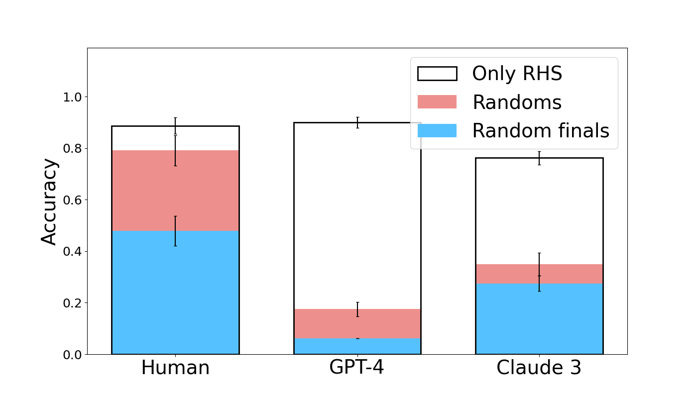Both humans and models competently complete the Only RHS condition (see Figure 4). Accuracy is approximately 0.8 for Claude 3 with human subjects and GPT-4 slightly higher at 0.9. GPT-4 is not significantly different from humans in this condition (coef = 0.1178, z = 0.223, p = 0.824), and Claude 3 is worse than humans by a barely significant margin (coef = -0.9130, z = -1.994, p = 0.046). Thus, both humans and LLMs are able to complete the task without the guidance of the left hand side. Considering this, we look at the performance degradation associated with encountering incoherent semantic structure on the left hand side. Humans exhibit a modest decrease in accuracy of about 0.15 in the Random and Random Permuted Pairs conditions relative to defaults. Claude-3 and GPT-4, however, exhibit much larger drops: Claude 3 decreases by approximately 0.5 relative to Defaults, while GPT-4 decreases by 0.6 and 0.4 in the Random and Random Permuted Pairs conditions. Across these two conditions, both GPT-4 (coef = -2.1972, z = -5.211, p < 0.001) and Claude 3 (coef = -2.0680, z = -4.960, p < 0.001) perform significantly worse than humans. <details> <summary>extracted/5679376/Images/fig4_new.png Details</summary>  ### Visual Description ## Stacked Bar Chart: Accuracy Comparison Across Human and AI Models ### Overview The image displays a stacked bar chart comparing the accuracy of three entities—Human, GPT-4, and Claude 3—across three distinct performance categories. The chart is designed to show the composition of overall accuracy for each entity, broken down into contributions from "Only RHS," "Randoms," and "Random finals." ### Components/Axes * **Y-Axis:** Labeled "Accuracy," with a linear scale ranging from 0.0 to 1.0. Major tick marks are present at 0.0, 0.2, 0.4, 0.6, 0.8, and 1.0. * **X-Axis:** Categorical, listing three groups: "Human," "GPT-4," and "Claude 3." * **Legend:** Positioned in the top-right corner of the chart area. It defines three stacked components: * **Only RHS:** Represented by a white bar segment with a black outline. * **Randoms:** Represented by a pink/salmon-colored bar segment. * **Random finals:** Represented by a light blue bar segment. * **Error Bars:** Each colored segment within every bar has a vertical black error bar extending above and below its top edge, indicating variability or confidence intervals for that specific measurement. ### Detailed Analysis The chart presents the following approximate accuracy values for each entity, decomposed by category. Values are estimated from the visual scale. **1. Human** * **Total Accuracy (Top of White Bar):** ~0.89 * **Component Breakdown (from bottom to top):** * **Random finals (Blue):** ~0.48 * **Randoms (Pink):** ~0.31 (Cumulative height: ~0.79) * **Only RHS (White):** ~0.10 (Cumulative height: ~0.89) * **Trend:** The largest contributor to Human accuracy is "Random finals," followed by "Randoms." The "Only RHS" component is the smallest. **2. GPT-4** * **Total Accuracy (Top of White Bar):** ~0.90 * **Component Breakdown (from bottom to top):** * **Random finals (Blue):** ~0.06 * **Randoms (Pink):** ~0.12 (Cumulative height: ~0.18) * **Only RHS (White):** ~0.72 (Cumulative height: ~0.90) * **Trend:** The vast majority of GPT-4's accuracy comes from the "Only RHS" component. The contributions from "Random finals" and "Randoms" are minimal. **3. Claude 3** * **Total Accuracy (Top of White Bar):** ~0.77 * **Component Breakdown (from bottom to top):** * **Random finals (Blue):** ~0.28 * **Randoms (Pink):** ~0.07 (Cumulative height: ~0.35) * **Only RHS (White):** ~0.42 (Cumulative height: ~0.77) * **Trend:** Claude 3 shows a mixed profile. "Only RHS" is the largest single component, but "Random finals" also provides a substantial contribution. "Randoms" is the smallest component. ### Key Observations 1. **Divergent Strategies:** The three entities exhibit fundamentally different accuracy compositions. Humans rely heavily on "Random finals" and "Randoms," GPT-4 relies almost exclusively on "Only RHS," and Claude 3 uses a combination of both strategies. 2. **Performance Hierarchy:** In terms of total accuracy, GPT-4 (~0.90) and Human (~0.89) are nearly tied at the top, with Claude 3 (~0.77) performing lower. 3. **"Only RHS" Dominance in AI:** Both AI models (GPT-4 and Claude 3) derive a larger proportion of their accuracy from the "Only RHS" category compared to Humans. 4. **Error Bar Variability:** The error bars are most pronounced on the "Only RHS" segments for Human and GPT-4, suggesting greater uncertainty or variance in that specific measurement for those groups. The error bars on the smaller "Randoms" and "Random finals" segments for GPT-4 are relatively tight. ### Interpretation This chart likely visualizes the results of a benchmark or experiment testing reasoning or problem-solving capabilities. The categories suggest different methods or information sources: * **"Only RHS":** Possibly refers to using only the Right-Hand Side of an equation or a specific, constrained set of rules. * **"Random finals" / "Randoms":** Suggest strategies involving randomness, guessing, or less deterministic approaches. The data demonstrates that advanced AI models like GPT-4 can achieve human-level accuracy on this task, but they do so through a markedly different mechanism—leveraging a precise, rule-based approach ("Only RHS") rather than the more stochastic or heuristic methods ("Random finals"/"Randoms") that characterize human performance in this context. Claude 3 represents an intermediate state, blending both approaches but not excelling in either to the same degree as the specialists (Human in randomness, GPT-4 in rules). The high accuracy of GPT-4 with a low error bar on the "Only RHS" segment indicates a robust and reliable mastery of that specific method. </details> Figure 4: Human and LLM accuracy in Only RHS, Randoms, and Random finals conditions. Data from the Random Permuted Pairs condition is shown in Figure 15 of the Appendix . Error bars show standard errors. From this we conclude that human subjects are able to easily identify when the left hand side contains no useful semantic structure to leverage. When there is none, they are able to employ a strategy that only relies on the right hand side. By contrast, models do not seem capable of easily identifying the lack of informativeness of the left hand side in these conditions, as they do not use the strategy of only attending to the right hand side, even though they show their capability of using this strategy when no left hand side is present. This suggests mechanistic differences between how human subjects and models process this task. Although the performance of human subjects does not drop notably in the Random condition compared to the Only RHS condition, it does drop by a wide margin in the Random Finals condition. In this condition, accuracy is approximately 0.5 lower than in the Only RHS condition. This further suggests that the semantic relatedness of the left hand side affects the strategy of human subjects: when the left hand side is clearly unrelated, the information it provides is discarded, but when much of the left hand side appears related, the information is not discarded and the random final word of the source domain prompts an incorrect answer from human subjects. Models also show a large drop in performance in the Random Finals condition relative to Only RHS, with Claude 3 dropping by 0.5 and GPT-4 dropping by 0.8. Simple effects analysis shows that both Claude 3 (coef = -1.0464, z = -2.799, p = 0.005) and GPT-4 (coef = -2.7850, z = -5.168, p < 0.001) are significantly worse than humans in the Random Finals condition. However, we see this difference as less informative than that both models drop in performance across all the random conditions relative to their own performance in the Only RHS condition. #### 3.1.3 Other Observations We additionally analyze the extent to which human subjects and models improve by question (Figure 14 of the Appendix), and the extent to which the errors made by humans and models follow the same distribution across questions grouped by target domain and across qualitative error types (Figure 13 and Table 5 of the Appendix). We find that humans and models alike improve over subsequent questions, adding to a body of evidence about in-context learning [30, 31, 32]. Humans and models show similar error distributions by target domain, but qualitative error types reveal a closer correspondence between human and GPT-4 errors than Claude 3. #### 3.1.4 Diagnosing the Use of an RHS-Only Heuristic To clarify whether subjects actually make use of left-right relations or only complete right-side patterns in the Semantic Structure experiment, we design the Relational condition, a $2× n$ variant of the Defaults condition which cannot be solved (consistently) using only the right-hand terms (see the example in Table 3). | pants => H # H | | --- | | glove => X # X | | torso => V | | foot => Z | | head => M | | shirt => V # V | | hat => | Table 3: An example from the Relational variant of the Defaults task, used to diagnose subjects’ tendency to rely on RHS-only heuristics to solve the task. 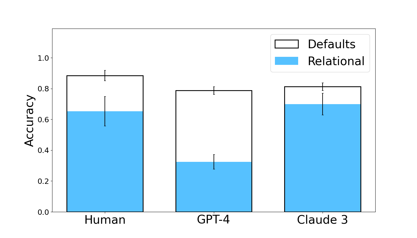Results are shown in Figure 5. Human subjects and Claude 3 exhibit similar performance, with accuracies of approximately 0.7. GPT-4, however, attains much lower accuracy of approximately 0.35. Simple effects analysis shows that GPT-4 obtains significantly worse accuracy than human subjects (coef = -1.3669, z = -3.065, p = 0.002), while the accuracy of Claude 3 does not differ significantly from human subjects (coef = 0.2111, z = 0.467, p = 0.640). <details> <summary>extracted/5679376/Images/fig5_new.png Details</summary>  ### Visual Description ## Bar Chart: Accuracy Comparison of Defaults vs. Relational Tasks ### Overview The image is a grouped bar chart comparing the accuracy of three entities—Human, GPT-4, and Claude 3—on two types of tasks: "Defaults" and "Relational." The chart includes error bars for each data point, indicating variability or confidence intervals. The overall visual suggests a performance comparison between human and AI model capabilities on different cognitive task types. ### Components/Axes * **Y-Axis:** Labeled "Accuracy." The scale runs from 0.0 to 1.0, with major tick marks at 0.0, 0.2, 0.4, 0.6, 0.8, and 1.0. * **X-Axis:** Categorical, listing three entities: "Human," "GPT-4," and "Claude 3." * **Legend:** Located in the top-right corner of the chart area. * **Defaults:** Represented by a white bar with a black outline. * **Relational:** Represented by a solid light blue bar. * **Data Series:** For each entity on the x-axis, there are two adjacent bars: a white "Defaults" bar and a blue "Relational" bar. Each bar has a vertical error bar extending above and below its top edge. ### Detailed Analysis **1. Human:** * **Defaults (White Bar):** The bar height is approximately **0.88**. The error bar extends from roughly **0.85 to 0.92**. * **Relational (Blue Bar):** The bar height is approximately **0.65**. The error bar is larger, extending from roughly **0.56 to 0.75**. * **Trend:** Human accuracy is significantly higher on Defaults tasks than on Relational tasks. **2. GPT-4:** * **Defaults (White Bar):** The bar height is approximately **0.79**. The error bar is relatively small, extending from roughly **0.77 to 0.81**. * **Relational (Blue Bar):** The bar height is approximately **0.32**. The error bar extends from roughly **0.28 to 0.37**. * **Trend:** GPT-4 shows a very large performance drop from Defaults to Relational tasks, with Relational accuracy being less than half of its Defaults accuracy. **3. Claude 3:** * **Defaults (White Bar):** The bar height is approximately **0.81**. The error bar extends from roughly **0.79 to 0.83**. * **Relational (Blue Bar):** The bar height is approximately **0.70**. The error bar extends from roughly **0.63 to 0.77**. * **Trend:** Claude 3 also performs better on Defaults than Relational tasks, but the gap is smaller than that observed for GPT-4. ### Key Observations 1. **Universal Performance Gap:** All three entities (Human, GPT-4, Claude 3) achieve higher accuracy on "Defaults" tasks compared to "Relational" tasks. 2. **Magnitude of Gap Varies:** The performance gap between task types is most extreme for GPT-4, moderate for Humans, and smallest for Claude 3. 3. **Relative Performance:** * On **Defaults** tasks, Humans (~0.88) have the highest accuracy, followed closely by Claude 3 (~0.81) and then GPT-4 (~0.79). * On **Relational** tasks, Claude 3 (~0.70) has the highest accuracy, followed by Humans (~0.65), with GPT-4 (~0.32) performing substantially worse. 4. **Error Bar Variability:** The error bars for "Relational" tasks are generally larger than those for "Defaults" tasks, particularly for Human and Claude 3, suggesting greater variability or uncertainty in performance on relational reasoning. ### Interpretation The data suggests a fundamental distinction in capability between "Defaults" (likely factual recall or common-sense knowledge) and "Relational" (likely involving reasoning about relationships between entities or concepts) tasks. * **Human Performance:** Humans show a robust but not perfect ability in both domains, with a notable drop in accuracy when relational reasoning is required. The larger error bar on the relational task indicates this is a more variable skill among humans. * **AI Model Divergence:** The two AI models exhibit starkly different profiles. **GPT-4** demonstrates strong performance on Defaults, nearly matching humans, but fails dramatically on Relational tasks. This implies its knowledge base is extensive, but its capacity for structured relational reasoning is a significant weakness. * **Claude 3's Profile:** **Claude 3** shows a more balanced profile. While slightly less accurate than humans on Defaults, it outperforms humans on the Relational task in this sample and maintains a much smaller performance gap between the two task types. This suggests a stronger architectural or training emphasis on relational reasoning compared to GPT-4. * **Overall Implication:** The chart highlights that "accuracy" is not a monolithic metric. An AI's performance is highly dependent on the *type* of cognitive task. Claude 3 appears more robust for tasks requiring relational understanding, while GPT-4's strength lies in default knowledge retrieval. The human benchmark provides a reference point for a balanced, albeit imperfect, integration of both capabilities. </details> Figure 5: Human and LLM accuracy in the Relational condition followup, with Defaults condition performance for reference. Error bars show standard errors. #### 3.1.5 Takeaways Despite weak performance from many models on our analogical reasoning tasks, GPT-4 and Claude 3 perform well, showing similar patterns to humans in leveraging semantic structure of corresponding domains to solve analogies. However, differences do remain in how they handle semantic structure in the source domain. Humans prefer leveraging semantic structure when a clear pattern exists (evidenced by the Defaults and Random Finals conditions) but can ignore words when structure is lacking (Randoms condition). Models show the former bias but not the latter ability, appearing distracted by random lexical items. Nevertheless, model results increasingly resemble human subjects, suggesting larger models may close this gap. Furthermore, qualitative differences exist even between the best models. GPT-4 and Claude 3 match human performance in the Defaults condition, but when the structure is generalized from $2× 2$ to $2× n$ in the Relational followup, making a right-hand-only strategy unworkable, Claude 3 maintains human-level performance while GPT-4 drops significantly. Despite limited public information, it’s notable that models produced using presumably similar approaches can exhibit meaningfully different behavioral patterns. ### 3.2 Mapping Semantic Content The Semantic Structure experiment, which presented subjects with source and target domains with corresponding semantic structure (i.e., with corresponding relations between terms), provides insight into the relative bias of human subjects and models to transfer this structure across domains. The Semantic Content experiment modifies the tasks to investigate the extent to which human subjects and models can transfer elements of the linguistic meaning of terms from one domain to another. To achieve this, we ensure that elements of the target domain directly depend on properties of corresponding source domain elements, requiring knowledge of the source domain terms’ meaning for perfect performance. As in the Semantic Structure experiment, source and target domains are paired such that patterns in the target domain mirror those in the source domain. Together, these experiments compare the subject’s ability and tendency to use a structure-mapping approach. Four tasks are generated, encoding either one or two dimensions of variation and either involving or not involving numeric reasoning (see Table 4). | Categorial: Right-hand terms are single characters corresponding to a Categorial property of the left-hand terms. | chicken => ! spider => ! cat => * horse => * ant => ! dog => * bee => ! human => | | --- | --- | | Multi-Attribute: Right-hand terms are a sequence of several characters that vary according to two properties of the left-hand terms. | grandfather => ! grandmother => * mother => * * father => ! ! brother => ! ! ! sister => | | Numeric: Right-hand terms are a sequence of a single repeated character, with the number of repetitions corresponding to a numeric property of the left-hand terms. | chicken => * * human => * * dog => * * * * spider => * * * * * * * * cat => * * * * horse => * * * * bee => | | Numeric Multi-Attribute: Right-hand terms are a sequence of a repeated character, with the number of repetitions corresponding to a numeric property of the left-hand terms and the character corresponding to a Categorial property. | horse => * * * * cat => * * * * ant => ! ! ! ! ! ! bee => ! ! ! ! ! ! chicken => ! ! spider => ! ! ! ! ! ! ! ! dog => * * * * human => | Table 4: The conditions of the Semantic Content experiment. <details> <summary>extracted/5679376/Images/exp2_new.png Details</summary>  ### Visual Description ## Grouped Bar Chart: Accuracy Comparison of Human and AI Models on Attribute Tasks ### Overview The image is a grouped bar chart comparing the accuracy of three entities—Human, GPT-4, and Claude 3—on tasks involving different attribute types. The chart measures performance on "Single attribute," "Numeric," and "Categorical" tasks, with accuracy plotted on the y-axis. Error bars are included for each data point, indicating variability or confidence intervals. ### Components/Axes - **Chart Type**: Grouped bar chart with error bars. - **Y-Axis**: Labeled "Accuracy," with a linear scale from 0.0 to 1.0, marked at intervals of 0.2 (0.0, 0.2, 0.4, 0.6, 0.8, 1.0). - **X-Axis**: Three categorical groups: "Human," "GPT-4," and "Claude 3." - **Legend**: Located in the top-right corner of the chart area. It defines three bar types: - **Single attribute**: White bar with a black outline. - **Numeric**: Solid pink/salmon-colored bar. - **Categorical**: Solid light blue bar. - **Data Series**: Each group (Human, GPT-4, Claude 3) contains two or three bars, representing the attribute types. The "Single attribute" bar appears only for Human and Claude 3, not for GPT-4. ### Detailed Analysis **Human Group (Leftmost Cluster):** - **Categorical (Blue Bar)**: Height is approximately 0.45. The error bar extends from roughly 0.36 to 0.53. - **Numeric (Pink Bar)**: Height is approximately 0.50. The error bar extends from roughly 0.44 to 0.56. - **Single attribute (White Bar)**: Height is approximately 0.73. The error bar extends from roughly 0.67 to 0.80. **GPT-4 Group (Center Cluster):** - **Categorical (Blue Bar)**: Height is approximately 0.70. The error bar extends from roughly 0.63 to 0.74. - **Numeric (Pink Bar)**: Height is approximately 0.25. The error bar extends from roughly 0.22 to 0.29. - **Single attribute**: No bar is present for this category. **Claude 3 Group (Rightmost Cluster):** - **Categorical (Blue Bar)**: Height is approximately 0.60. The error bar extends from roughly 0.52 to 0.62. - **Numeric (Pink Bar)**: Height is approximately 0.45. The error bar extends from roughly 0.42 to 0.47. - **Single attribute (White Bar)**: Height is approximately 0.55. The error bar extends from roughly 0.51 to 0.58. ### Key Observations 1. **Performance Disparity by Task Type**: There is a clear divergence in performance between Numeric and Categorical tasks for the AI models. GPT-4 shows the largest gap, with high Categorical accuracy (~0.70) but very low Numeric accuracy (~0.25). Humans show a smaller gap, with Numeric (~0.50) slightly outperforming Categorical (~0.45). 2. **Human Superiority on Single Attribute Tasks**: The "Single attribute" task, which appears to be a composite or different benchmark, shows Humans achieving the highest overall accuracy (~0.73) on the chart. Claude 3's performance on this task (~0.55) is notably lower. 3. **Model Comparison**: GPT-4 leads in Categorical accuracy among the AI models. Claude 3 shows more balanced performance between Numeric and Categorical tasks compared to GPT-4, but its accuracy in both is moderate. 4. **Error Bar Variability**: The error bars for Human performance on Categorical tasks and GPT-4 performance on Numeric tasks appear relatively large, suggesting higher uncertainty or variability in those measurements. Claude 3's error bars are comparatively tighter. ### Interpretation This chart suggests a fundamental difference in how humans and current large language models (LLMs) process different types of information. Humans demonstrate a more balanced and robust capability across numeric and categorical reasoning, with a particular strength in integrated "single attribute" tasks. The LLMs, however, show a pronounced specialization or weakness. GPT-4's profile indicates a strong capability for categorical reasoning (e.g., classifying, sorting) but a significant deficit in numeric reasoning (e.g., arithmetic, quantitative comparison). Claude 3 mitigates this weakness somewhat, achieving a more even performance profile, but at the cost of lower peak accuracy in its stronger category compared to GPT-4. The absence of a "Single attribute" bar for GPT-4 is notable. It could imply that this specific benchmark was not run for GPT-4, or that the task was not applicable to its evaluation framework. The data highlights that while AI models can excel in specific domains (like GPT-4 in categorical tasks), they have not yet achieved the generalized, cross-domain accuracy of humans, particularly in tasks that may require integrating multiple reasoning skills. The variability indicated by the error bars also suggests that model performance on these tasks is not yet fully consistent. 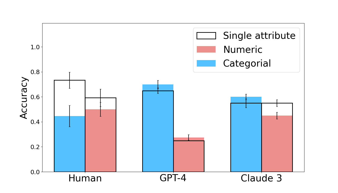</details> Figure 6: Human and model accuracy by condition in the Semantic Content experiment. Error bars show standard errors. Results for human subjects, GPT-4, and Claude 3 are shown in Figure 6 (other tested models attain much lower accuracy as before). #### 3.2.1 Human Performance Continues to be Robust Human subjects perform robustly and consistently, as in the previous experiment. Human accuracy ranges from 0.4 to 0.8 across conditions, comparable to the earlier Semantic Structure experiment. As expected, subjects generally describe their strategy as relating properties of the left-hand terms to their representations on the right-hand side. #### 3.2.2 Claude 3 Matches Human Performance Stably Across Conditions Claude 3 matches human performance stably across the different conditions of the Semantic Content experiment with its accuracy falling into a comparable range of 0.4 to 0.7. The model exhibits marginally better performance in the Multi-Attribute condition and marginally worse performance in the remaining three. These differences are insignificant across all conditions, which covers the Categorial (coef = -0.8109, z = -1.879, p = 0.060), Multi-Attribute (coef = 0.6206, z = 1.478, p = 0.140), Numeric (coef = -0.1788, z = -0.439, p = 0.661), and Numeric Multi-Attribute (coef = -0.2009, z = -0.484, p = 0.629) conditions. Therefore, Claude 3 performs as well as human subjects across all conditions of this experiment. #### 3.2.3 GPT-4 Lags Human Subjects on Numeric Reasoning GPT-4 achieves good results in the Categorial and Multi-Attribute conditions, with mean accuracies of approximately 0.7 in both (compared to 0.7 and 0.4 respectively for human subjects). GPT-4 is not significantly worse than humans in the Categorial condition (coef = -0.3927, z = -0.889, p = 0.374). GPT-4 significantly outperforms human subjects in the Multi-Attribute condition (coef = 1.0624, z = 2.429, p = 0.015). However, its accuracy drops to 0.2-0.3 in the remaining conditions and we find that GPT-4 is significantly worse than humans in both the Numeric (coef = -1.4781, z = -3.321, p = 0.001) and Numeric Multi-Attribute conditions (coef = -0.9694, z = -2.185, p = 0.029). In these conditions, GPT-4 fails to correctly relate the number of characters in a response to the numeric property of the object (see Table 7 for an illustrative example). GPT-4’s failure to reason about the number of characters in the expected way is further observed in the sanity check shown in Table 8 of the Appendix, even when the model is not required to relate a property of a word to its representation. #### 3.2.4 Human Performance Drops in Compositional Conditions, But Models Remain Constant When comparing the performance of a subject in a non-compositional (single-attribute) condition to the corresponding compositional (multi-attribute) version, we observe some decrease in performance for human subjects but not for models (note that this surprising result is subject to alternative explanations, addressed in the discussion below). The accuracy of human subjects drops from approximately 0.7 to approximately 0.4 when comparing the Categorial condition to the corresponding compositional version (the Multi-Attribute condition). A simple effects analysis confirms that this decline is significant (coef = -1.2267, z = -3.091, p = 0.002). We see a non-significant decrease in accuracy for human subjects when comparing the Numeric condition to its compositional counterpart, with performance dropping from approximately 0.6 to approximately 0.5 (coef = -0.3795, z = -1.028, p = 0.304). By contrast, we do not find either model to be significantly worse in compositional conditions than non-compositional ones. In fact, GPT-4 exhibits a slight improvement in the compositional conditions, though this change is statistically insignificant for both the Multi-Attribute condition relative to the Categorial condition (coef = 0.2281, z = 0.477, p = 0.634) and for the Numeric Multi-Attribute condition relative to the Numeric condition (coef = 0.1292, z = 0.254, p = 0.799). For Claude 3 we similarly find the differences to be insignificant for the Multi-Attribute condition relative to the Categorial condition (coef = 0.2049, z = 0.452, p = 0.651) and for the Numeric Multi-Attribute condition relative to the Numeric condition (coef = -0.4013, z = -0.893, p = 0.372). #### 3.2.5 Takeaways The Semantic Content experiment confirms that human subjects perform robustly and flexibly across diverse task variations. Claude 3 matches human performance in all conditions, indicating it shares humans’ tendency to use the source domain’s semantic content when completing target domains. While GPT-4’s poor performance in numeric conditions is notable, it reflects a failure in numeric reasoning rather than a difference in analogical reasoning. We find evidence of decreased human performance, but not model performance, in compositional conditions, contrasting with some existing research [33]. However, other factors may be at play. Models’ negative compositionality effect may be masked by a positive effect, such as increased available information: when the target domain represents two source domain properties, models may more easily recognize the encoding of source domain properties. Human subjects may benefit less from this competing effect if they do not struggle to observe this information encoding. ## 4 Discussion Our results show that the best-performing LLMs are able to successfully complete many analogical reasoning tasks with human-level accuracy using novel stimuli not present in their training data. They also show that there remain meaningful differences in how such analogies are processed, evidenced by differences in how humans and models respond to distracting or misleading information. However, we observe a clear trend: more recent models come increasingly close to matching human performance across our tasks. In particular, Claude 3, the most recently-released model we test, exhibits impressively robust performance across most task variations, even closing the gap with humans in some test conditions in which its predecessor (GPT-4) exhibited limitations (such as the Relational task version in which mapping from the source domain must be used for success). Together, these results raise questions about the ability of LLMs and similar models to serve as candidate cognitive models, which we discuss briefly below. ### 4.1 Evaluating the Competence of LLMs The breadth of Claude 3’s success in our tasks is noteworthy. It suggests that state-of-the-art LLMs can broadly match human performance not only in formal analogical reasoning tasks, as suggested by Webb et al. [4], but also in tasks that require mapping semantic information across linguistic and non-linguistic domains. As such, our results weigh against a long-standing view in cognitive science, according to which connectionist models without a built-in symbolic component are constitutively limited in their ability to robustly handle analogical reasoning tasks [7]. They also inform discussions of whether LLMs possess “functional” linguistic competence, in addition to “formal” linguistic competence [3]. Further work is needed to characterize the precise mechanism that LLMs are using to solve these tasks; it is possible–though increasingly unlikely given the robustness of the behavioral results–that success is due to a myriad of heuristics rather than a systematic analogical reasoning process. Even so, evidence of LLMs completing analogical reasoning tasks in domains designed to involve linguistic structure-mapping, in addition to tasks over abstract symbols, runs counter to the claim that LLMs are capable of formal but not functional linguistic competence. There remain examples of LLMs performing much worse than humans on analogical reasoning tasks [10], which must be reconciled with our results. Here the competence-performance distinction, originally introduced by Noam Chomsky [34], can be usefully applied to the evaluation of LLMs [35, 2, 36]. This distinction allows researchers to theorize about the abstract computational principles governing cognition separately from the “noise” introduced by performance factors. In humans, it is generally assumed that there is a double dissociation between performance and competence: neither success nor failure on a task designed to measure a particular capacity can always be taken as conclusive evidence that subjects have or lack that capacity, due to auxiliary factors affecting task performance. When it comes to LLMs, by contrast, the distinction is typically applied in a single direction: human-like performance on benchmarks is often explained away by reliance on shallow heuristics [37] and/or lack of construct validity [38], while sub-human performance is often taken as reliable evidence of lack of competence. However, LLM performance can also be negatively affected by strong auxiliary task demands [39] and mismatched conditions in comparisons with human subjects [40]. These are compelling reasons to apply the dissociation in both directions to LLMs as well. From this perspective, our results offer evidence to support both sides of the present debate about whether LLMs possess human-level analogical reasoning (see Webb et al. [15], Mitchell et al. [10], and Hodel et al. [16]). Supporting the argument of Webb et al. [15] that deficiencies in capabilities other than analogical reasoning can explain poor model performance in some tasks, we find that GPT-4’s failure in the numeric conditions of our Semantic Content experiment may be due to a deficiency in counting ability. However, contrary to Webb et al. [4], who report impressive analogical reasoning in both GPT-3 and GPT-4, we do find a qualitative difference in the performance of these two models, with GPT-3 performing quite poorly on our tasks. Among the models tested, only GPT-4 and Claude 3 produce results that merit detailed comparison with human subjects. This suggests that claims of human-level performance of LLMs on analogical reasoning tasks may have been premature and might have relied on insufficiently challenging tasks. However, other differences we observe between human subjects and LLMs across task variations are not subject to an auxiliary task demand explanation and suggest that the underlying mechanisms of analogical reasoning in these systems may differ from that in humans. Importantly, these differences persist even in our best performing model, Claude 3. For instance, Claude 3 responds differently than human subjects when some or all words in the target domain are replaced with random words, indicating that they may use distinct strategies for identifying and leveraging relational similarities between source and target domains. Furthermore, Claude 3 remains more sensitive than human subjects to the ordering of elements within domains, which is difficult to explain if LLMs are using a generalizable symbolic working memory approach. Collectively, these patterns bear on the larger question of how we should arbitrate disputes about competence in machine-human comparisons. On the one hand, it seems reasonable to assume that any system that can reliably achieve success at or above human level on experiments like ours–without relying on memorization and other confounds–should be considered competent at analogical reasoning through structure-mapping. On the other hand, we should be open to the possibility that such competence may be implemented differently in LLMs and humans. The question of whether we require human-likeness of the mechanism to declare human-level “competence” is ultimately not empirical, but rather demands philosophical consensus among the scientific community around our ultimate goals and metrics for achieving them. ### 4.2 Analogy in Human(-like) Learning and Bootstrapping Unlike previous research comparing analogical reasoning in human subjects and LLMs, our tasks involve transferring semantic structure and content from source to target domains, rather than reasoning over abstract symbols. Our experiments thus investigate whether LLMs’ analogical reasoning resembles that of human subjects in a manner pertinent to its purportedly central role in broader cognition. Following Gentner [11], emphasis has been placed on relational similarity, rather than just feature similarity, in mapping from a familiar source to a foreign target domain during analogical reasoning to allow for the flexible transfer of knowledge [41, 42, 43]. This conception allows analogical reasoning to play a fundamental role in human cognition, supporting the emergence of diverse cognitive abilities via “bootstrapping” [44, 45, 46]. In bootstrapping, two cognitive processes mutually support each other’s development. In Gentner’s Structure-Mapping Theory (SMT), language development and structure-mapping-based analogical reasoning are hypothesized to co-develop, with structure-mapping developing the necessary relational reasoning to model language-world relations, and language acquisition in turn developing symbolic reasoning capacities that amplify structure-mapping abilities. Consequently, analogical reasoning is seen as a central cognitive phenomenon of interest. The success of some LLMs in many of our tasks suggests that the most advanced models may be capable of employing a structure-mapping based approach to analogical reasoning, in which relations in the source domain are used to constrain and guide reasoning about relations in the target domain. This raises the possibility that a bootstrapping cycle between language development and analogical reasoning in humans, as proposed by Gentner [44], may be paralleled in language models. The emergence of such competence from training primarily on text prediction would yield new hypotheses about the emergence of analogical reasoning as a central cognitive faculty from generic learning mechanisms (possibly combined with the unique pressures of language acquisition). However, the mixed success of LLMs and the significant differences from humans in certain conditions underscore the need for continued research to test the robustness of any conclusion that analogical reasoning in LLMs closely matches that of human subjects. As LLM outputs continue to converge toward human responses–an expected product of the language modelling objective–it is crucial to develop novel tasks that examine analogical reasoning ability and are not attested in the training data. While our task allows for clear discrimination between human performance and that of most models prior to Claude 3, further differences in analogical reasoning patterns between humans and Claude 3 likely exist beyond those revealed by our tests. More granular testing would help clarify the extent of the remaining discrepancies between humans and the most advanced LLMs, and much further work is required to verify the hypothesis that language models parallel the bootstrapping cycle between language development and analogical reasoning in humans. The proprietary nature of leading LLMs like Claude 3 unfortunately limits our ability to directly investigate the features that may explain the emergence of a response pattern largely mirroring that of human subjects. However, increasingly sophisticated open-weights models are being released, which may allow for interpretability work to analyze the internal mechanisms of a model and shed light on the underlying mechanisms that enable advanced LLMs to exhibit impressive analogical reasoning abilities in many tasks. ## 5 Acknowledgments This work was supported in part by NIH NIGMS COBRE grant #5P20GM10364510. ## References - [1] A. Srivastava, A. Rastogi, A. Rao, A. A. M. S. E. al., Beyond the imitation game: Quantifying and extrapolating the capabilities of language models (2023). arXiv:2206.04615. - [2] E. Pavlick, Symbols and grounding in large language models, Philosophical Transactions of the Royal Society A: Mathematical, Physical and Engineering Sciences 381 (2251) (Jun. 2023). doi:10.1098/rsta.2022.0041. URL http://dx.doi.org/10.1098/rsta.2022.0041 - [3] K. Mahowald, A. A. Ivanova, I. A. Blank, N. Kanwisher, J. B. Tenenbaum, E. Fedorenko, Dissociating language and thought in large language models (2023). arXiv:2301.06627. - [4] T. Webb, K. J. Holyoak, H. Lu, Emergent analogical reasoning in large language models, Nature Human Behaviour 7 (9) (2023) 1526––1541. - [5] S. J. Han, K. Ransom, A. Perfors, C. Kemp, Inductive reasoning in humans and large language models (2023). arXiv:2306.06548. - [6] X. Hu, S. Storks, R. L. Lewis, J. Chai, In-context analogical reasoning with pre-trained language models (2023). arXiv:2305.17626. - [7] M. Mitchell, Abstraction and analogy-making in artificial intelligence, Annals of the New York Academy of Sciences 1505 (1) (2021) 79–101. arXiv:https://nyaspubs.onlinelibrary.wiley.com/doi/pdf/10.1111/nyas.14619, doi:https://doi.org/10.1111/nyas.14619. URL https://nyaspubs.onlinelibrary.wiley.com/doi/abs/10.1111/nyas.14619 - [8] K. J. Holyoak, D. Gentner, B. N. Kokinov, Introduction: The Place of Analogy in Cognition, in: The Analogical Mind: Perspectives from Cognitive Science, The MIT Press, 2001. arXiv:https://direct.mit.edu/book/chapter-pdf/2323335/9780262316057\_caa.pdf, doi:10.7551/mitpress/1251.003.0003. URL https://doi.org/10.7551/mitpress/1251.003.0003 - [9] D. R. Hofstadter, Epilogue: Analogy as the Core of Cognition, in: The Analogical Mind: Perspectives from Cognitive Science, The MIT Press, 2001. arXiv:https://direct.mit.edu/book/chapter-pdf/2323391/9780262316057\_cao.pdf, doi:10.7551/mitpress/1251.003.0020. URL https://doi.org/10.7551/mitpress/1251.003.0020 - [10] M. Lewis, M. Mitchell, Using counterfactual tasks to evaluate the generality of analogical reasoning in large language models (2024). arXiv:2402.08955. - [11] D. Gentner, Structure-mapping: A theoretical framework for analogy*, Cognitive Science 7 (2) (1983) 155–170. arXiv:https://onlinelibrary.wiley.com/doi/pdf/10.1207/s15516709cog0702_3, doi:https://doi.org/10.1207/s15516709cog0702\_3. URL https://onlinelibrary.wiley.com/doi/abs/10.1207/s15516709cog0702_3 - [12] K. Erk, Towards a semantics for distributional representations, in: A. Koller, K. Erk (Eds.), Proceedings of the 10th International Conference on Computational Semantics (IWCS 2013) – Long Papers, Association for Computational Linguistics, Potsdam, Germany, 2013, pp. 95–106. URL https://aclanthology.org/W13-0109 - [13] G. Boleda, Distributional semantics and linguistic theory, CoRR abs/1905.01896 (2019). arXiv:1905.01896. URL http://arxiv.org/abs/1905.01896 - [14] L. Gleitman, C. Fisher, 6 universal aspects of word learning, in: J. A. McGilvray (Ed.), The Cambridge Companion to Chomsky, Cambridge University Press, 2005, p. 123. - [15] T. Webb, K. J. Holyoak, H. Lu, Evidence from counterfactual tasks supports emergent analogical reasoning in large language models (2024). arXiv:2404.13070. - [16] D. Hodel, J. West, Response: Emergent analogical reasoning in large language models (2024). arXiv:2308.16118. - [17] S. French, A model-theoretic account of representation (or, i don’t know much about art…but i know it involves isomorphism), Philosophy of Science 70 (5) (2003) 1472–1483. doi:10.1086/377423. - [18] T. B. Brown, B. Mann, N. Ryder, M. Subbiah, J. Kaplan, P. Dhariwal, A. Neelakantan, P. Shyam, G. Sastry, A. Askell, S. Agarwal, A. Herbert-Voss, G. Krueger, T. Henighan, R. Child, A. Ramesh, D. M. Ziegler, J. Wu, C. Winter, C. Hesse, M. Chen, E. Sigler, M. Litwin, S. Gray, B. Chess, J. Clark, C. Berner, S. McCandlish, A. Radford, I. Sutskever, D. Amodei, Language models are few-shot learners (2020). arXiv:2005.14165. - [19] OpenAI, J. Achiam, S. Adler, S. Agarwal, L. Ahmad, I. Akkaya, F. L. Aleman, D. Almeida, J. Altenschmidt, S. Altman, S. Anadkat, R. Avila, I. Babuschkin, S. Balaji, V. Balcom, P. Baltescu, H. Bao, M. Bavarian, J. Belgum, I. Bello, J. Berdine, G. Bernadett-Shapiro, C. Berner, L. Bogdonoff, O. Boiko, M. Boyd, A.-L. Brakman, G. Brockman, T. Brooks, M. Brundage, K. Button, T. Cai, R. Campbell, A. Cann, B. Carey, C. Carlson, R. Carmichael, B. Chan, C. Chang, F. Chantzis, D. Chen, S. Chen, R. Chen, J. Chen, M. Chen, B. Chess, C. Cho, C. Chu, H. W. Chung, D. Cummings, J. Currier, Y. Dai, C. Decareaux, T. Degry, N. Deutsch, D. Deville, A. Dhar, D. Dohan, S. Dowling, S. Dunning, A. Ecoffet, A. Eleti, T. Eloundou, D. Farhi, L. Fedus, N. Felix, S. P. Fishman, J. Forte, I. Fulford, L. Gao, E. Georges, C. Gibson, V. Goel, T. Gogineni, G. Goh, R. Gontijo-Lopes, J. Gordon, M. Grafstein, S. Gray, R. Greene, J. Gross, S. S. Gu, Y. Guo, C. Hallacy, J. Han, J. Harris, Y. He, M. Heaton, J. Heidecke, C. Hesse, A. Hickey, W. Hickey, P. Hoeschele, B. Houghton, K. Hsu, S. Hu, X. Hu, J. Huizinga, S. Jain, S. Jain, J. Jang, A. Jiang, R. Jiang, H. Jin, D. Jin, S. Jomoto, B. Jonn, H. Jun, T. Kaftan, Łukasz Kaiser, A. Kamali, I. Kanitscheider, N. S. Keskar, T. Khan, L. Kilpatrick, J. W. Kim, C. Kim, Y. Kim, J. H. Kirchner, J. Kiros, M. Knight, D. Kokotajlo, Łukasz Kondraciuk, A. Kondrich, A. Konstantinidis, K. Kosic, G. Krueger, V. Kuo, M. Lampe, I. Lan, T. Lee, J. Leike, J. Leung, D. Levy, C. M. Li, R. Lim, M. Lin, S. Lin, M. Litwin, T. Lopez, R. Lowe, P. Lue, A. Makanju, K. Malfacini, S. Manning, T. Markov, Y. Markovski, B. Martin, K. Mayer, A. Mayne, B. McGrew, S. M. McKinney, C. McLeavey, P. McMillan, J. McNeil, D. Medina, A. Mehta, J. Menick, L. Metz, A. Mishchenko, P. Mishkin, V. Monaco, E. Morikawa, D. Mossing, T. Mu, M. Murati, O. Murk, D. Mély, A. Nair, R. Nakano, R. Nayak, A. Neelakantan, R. Ngo, H. Noh, L. Ouyang, C. O’Keefe, J. Pachocki, A. Paino, J. Palermo, A. Pantuliano, G. Parascandolo, J. Parish, E. Parparita, A. Passos, M. Pavlov, A. Peng, A. Perelman, F. de Avila Belbute Peres, M. Petrov, H. P. de Oliveira Pinto, Michael, Pokorny, M. Pokrass, V. H. Pong, T. Powell, A. Power, B. Power, E. Proehl, R. Puri, A. Radford, J. Rae, A. Ramesh, C. Raymond, F. Real, K. Rimbach, C. Ross, B. Rotsted, H. Roussez, N. Ryder, M. Saltarelli, T. Sanders, S. Santurkar, G. Sastry, H. Schmidt, D. Schnurr, J. Schulman, D. Selsam, K. Sheppard, T. Sherbakov, J. Shieh, S. Shoker, P. Shyam, S. Sidor, E. Sigler, M. Simens, J. Sitkin, K. Slama, I. Sohl, B. Sokolowsky, Y. Song, N. Staudacher, F. P. Such, N. Summers, I. Sutskever, J. Tang, N. Tezak, M. B. Thompson, P. Tillet, A. Tootoonchian, E. Tseng, P. Tuggle, N. Turley, J. Tworek, J. F. C. Uribe, A. Vallone, A. Vijayvergiya, C. Voss, C. Wainwright, J. J. Wang, A. Wang, B. Wang, J. Ward, J. Wei, C. Weinmann, A. Welihinda, P. Welinder, J. Weng, L. Weng, M. Wiethoff, D. Willner, C. Winter, S. Wolrich, H. Wong, L. Workman, S. Wu, J. Wu, M. Wu, K. Xiao, T. Xu, S. Yoo, K. Yu, Q. Yuan, W. Zaremba, R. Zellers, C. Zhang, M. Zhang, S. Zhao, T. Zheng, J. Zhuang, W. Zhuk, B. Zoph, Gpt-4 technical report (2024). arXiv:2303.08774. - [20] S. Biderman, H. Schoelkopf, Q. Anthony, H. Bradley, K. O’Brien, E. Hallahan, M. A. Khan, S. Purohit, U. S. Prashanth, E. Raff, A. Skowron, L. Sutawika, O. van der Wal, Pythia: A suite for analyzing large language models across training and scaling (2023). arXiv:2304.01373. - [21] Anthropic, Claude-2 language model, https://www.anthropic.com/index/claude-2, accessed: 2023-11-06 (2023). - [22] Anthropic, The Claude 3 Model Family: Opus, Sonnet, Haiku, https://www-cdn.anthropic.com/de8ba9b01c9ab7cbabf5c33b80b7bbc618857627/Model_Card_Claude_3.pdf, accessed: 2024-05-01 (2024). - [23] Technology Innovation Institute, Falcon language model, https://falconllm.tii.ae/falcon.html, accessed: 2023-10-31 (2023). - [24] B. Liu, L. Ding, L. Shen, K. Peng, Y. Cao, D. Cheng, D. Tao, Diversifying the mixture-of-experts representation for language models with orthogonal optimizer (2023). arXiv:2310.09762. - [25] S. Glover, P. Dixon, Likelihood ratios: A simple and flexible statistic for empirical psychologists, Psychonomic Bulletin & Review 11 (5) (2004) 791–806. doi:10.3758/BF03196706. URL https://doi.org/10.3758/BF03196706 - [26] P. Carvalho, R. Goldstone, Category structure modulates interleaving and blocking advantage in inductive category acquisition, in: Proceedings of the 34th Annual Conference of the Cognitive Science Society, 2012, pp. 186–191. - [27] J. Russin, E. Pavlick, M. J. Frank, Human curriculum effects emerge with in-context learning in neural networks (2024). arXiv:2402.08674. - [28] D. Hendrycks, C. Burns, S. Basart, A. Zou, M. Mazeika, D. Song, J. Steinhardt, Measuring massive multitask language understanding (2021). arXiv:2009.03300. - [29] J. Kaplan, S. McCandlish, T. Henighan, T. B. Brown, B. Chess, R. Child, S. Gray, A. Radford, J. Wu, D. Amodei, Scaling laws for neural language models (2020). arXiv:2001.08361. - [30] S. M. Xie, A. Raghunathan, P. Liang, T. Ma, An explanation of in-context learning as implicit bayesian inference (2022). arXiv:2111.02080. - [31] Y. Zhang, F. Zhang, Z. Yang, Z. Wang, What and how does in-context learning learn? bayesian model averaging, parameterization, and generalization (2023). arXiv:2305.19420. - [32] A. Raventós, M. Paul, F. Chen, S. Ganguli, Pretraining task diversity and the emergence of non-bayesian in-context learning for regression, in: A. Oh, T. Naumann, A. Globerson, K. Saenko, M. Hardt, S. Levine (Eds.), Advances in Neural Information Processing Systems, Vol. 36, Curran Associates, Inc., 2023, pp. 14228–14246. URL https://proceedings.neurips.cc/paper_files/paper/2023/file/2e10b2c2e1aa4f8083c37dfe269873f8-Paper-Conference.pdf - [33] O. Press, M. Zhang, S. Min, L. Schmidt, N. A. Smith, M. Lewis, Measuring and narrowing the compositionality gap in language models (2023). arXiv:2210.03350. - [34] N. Chomsky, Aspects of the Theory of Syntax, 50th Edition, The MIT Press, 1965. URL http://www.jstor.org/stable/j.ctt17kk81z - [35] C. Firestone, Performance vs. competence in human-machine comparisons, Proc Natl Acad Sci U S A 117 (43) (2020) 26562–26571. - [36] E. Pavlick, Semantic structure in deep learning (january 2022), Annual Review of Linguistics 8 (2022) 447–471. URL http://dx.doi.org/10.1146/annurev-linguistics-031120-122924 - [37] R. T. McCoy, S. Yao, D. Friedman, M. Hardy, T. L. Griffiths, Embers of autoregression: Understanding large language models through the problem they are trained to solve (2023). arXiv:2309.13638. - [38] T. Ullman, Large language models fail on trivial alterations to theory-of-mind tasks (2023). arXiv:2302.08399. - [39] J. Hu, M. C. Frank, Auxiliary task demands mask the capabilities of smaller language models (2024). arXiv:2404.02418. - [40] A. K. Lampinen, Can language models handle recursively nested grammatical structures? a case study on comparing models and humans (2023). arXiv:2210.15303. - [41] H. Gust, U. Krumnack, K.-U. Kühnberger, A. Schwering, Analogical reasoning: A core of cognition., KI 22 (2008) 8–12. - [42] G. S. Halford, W. H. Wilson, S. Phillips, Relational knowledge: the foundation of higher cognition, Trends in Cognitive Sciences 14 (11) (2010) 497–505. doi:https://doi.org/10.1016/j.tics.2010.08.005. URL https://www.sciencedirect.com/science/article/pii/S1364661310002020 - [43] K. J. Holyoak, 234 Analogy and Relational Reasoning, in: The Oxford Handbook of Thinking and Reasoning, Oxford University Press, 2012. arXiv:https://academic.oup.com/book/0/chapter/293248246/chapter-ag-pdf/44513038/book\_34559\_section\_293248246.ag.pdf, doi:10.1093/oxfordhb/9780199734689.013.0013. URL https://doi.org/10.1093/oxfordhb/9780199734689.013.0013 - [44] D. Gentner, Bootstrapping the mind: Analogical processes and symbol systems, Cognitive Science 34 (5) (2010) 752–775. arXiv:https://onlinelibrary.wiley.com/doi/pdf/10.1111/j.1551-6709.2010.01114.x, doi:https://doi.org/10.1111/j.1551-6709.2010.01114.x. URL https://onlinelibrary.wiley.com/doi/abs/10.1111/j.1551-6709.2010.01114.x - [45] S. Carey, Bootstrapping & the origin of concepts, Daedalus 133 (1) (2004) 59–68. arXiv:https://direct.mit.edu/daed/article-pdf/133/1/59/1828762/001152604772746701.pdf, doi:10.1162/001152604772746701. URL https://doi.org/10.1162/001152604772746701 - [46] S. Carey, The Origin of Concepts, Oxford University Press, 2009. doi:10.1093/acprof:oso/9780195367638.001.0001. URL https://doi.org/10.1093/acprof:oso/9780195367638.001.0001 ## Appendix A Statistical outputs and supplementary figures ### A.1 Regression results, Semantic Structure experiment We perform a logistic regression with the outcome variable being the raw score (a 0 or 1 for each question). The predictor variables are condition and subject type (restricted to human subjects and GPT-4 only, or human subjects and Claude 3 only). The regression is performed with and without interactions: Without interactions: $smf.logit(formula=respondent\_scores∼ C(subject\_type,Treatment(reference= human))+C(quiz\_class,Treatment(reference=permuted\_questions)),data=all\_ subjects\_df,).fit(maxiter=1000,method=bfgs)$ With interactions: $smf.logit(formula=respondent\_scores∼ C(subject\_type,Treatment(reference= human))*C(quiz\_class,Treatment(reference=permuted\_questions)),data=all\_ subjects\_df,).fit(maxiter=1000,method=bfgs)$ The significance of including the interaction between predictors is assessed with a likelihood ratio test with the associated p-value calculated as follows: $p=chi2.sf(lik\_ratio,degfree)$ , with 7 degrees of freedom. The likelihood ratio in the above formula is calculated as follows: $lik\_ratio=degfree*(res\_subjXclass.llf-res\_subjplusclass.llf)$ . In the above, res_subjXclass and res_subjplusclass are the regression outputs with and without interactions respectively. For both comparisons (human subjects compared to GPT-4 and human subjects compared to Claude 3), we find a significant improvement in model fit when interactions between the subject type and experiment condition are included.A likelihood ratio test shows that including interactions between subject type and experiment condition leads to a significantly better fit of the model ( $chi^2(7)=115.1871,p<0.001$ ). For the comparison between Claude 3 and human subjects, we again find a significant negative effect of the subject type being Claude 3 when interactions are not included (coef = -0.8706, z = -5.608, p < 0.001) and find that subject type - condition interactions are significant ( $chi^2(7)=173.6511,p<0.001$ ). These results are consistent with the observation that the two models exhibit variable performance across conditions, and indicate that the overall performance gap to human subjects is driven by low model accuracy in certain conditions. Simple effects analysis is used below to assess the effect of subject type in particular conditions and groups thereof. Regression outputs are shown in Figure 7 and 8. 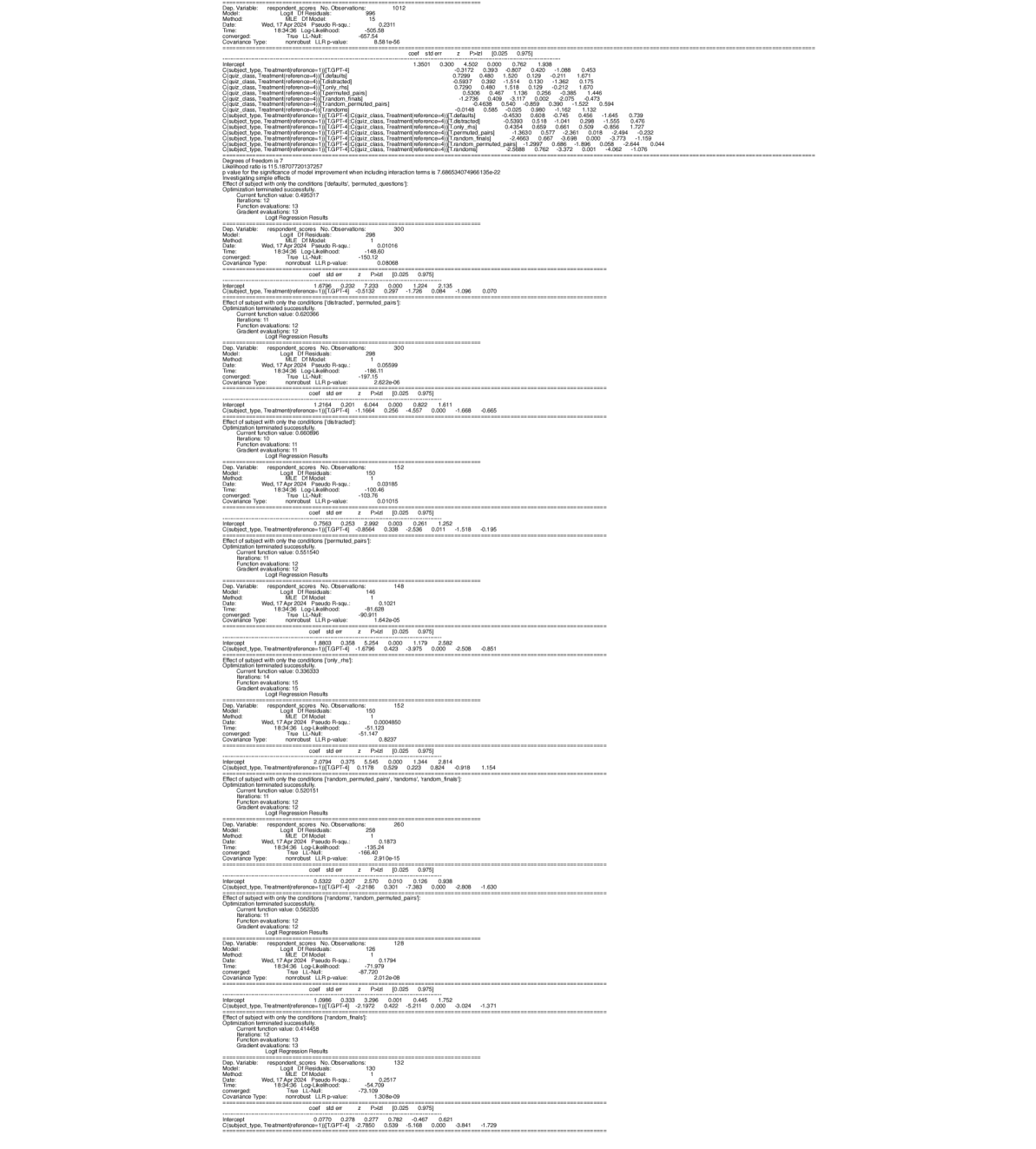<details> <summary>x1.png Details</summary>  ### Visual Description \n ## Logit Regression Output Series: Multi-Model Statistical Analysis ### Overview The image displays a vertical sequence of eight distinct statistical output blocks, each representing the results of a **Logit Regression** analysis. The outputs are generated from a statistical software package (likely Python's `statsmodels` or similar) and appear to be part of a larger analysis investigating the effect of a categorical variable (`C(subject_type, Treatment(reference=1))`) on a dependent variable (`respondent_scores`) under various conditions or subsets of data. The text is monospaced and presented in a standard console output format. ### Components/Axes The image is not a chart or diagram but a series of textual statistical reports. Each report block contains the following standard components: 1. **Header:** "Logit Regression Results" 2. **Model Information Table:** Includes: * `Dep. Variable:` (respondent_scores) * `Model:` (Logit) * `Method:` (MLE) * `Date:` (Wed, 17 Apr 2024) * `Time:` (18:34:36) * `No. Observations:` (varies per model) * `Df Residuals:` (varies) * `Df Model:` (varies) * `Pseudo R-squ.:` (varies) * `Log-Likelihood:` (varies) * `converged:` (True) * `Covariance Type:` (nonrobust) * `LLR p-value:` (varies) 3. **Coefficients Table:** Columns are: * `coef` (coefficient) * `std err` (standard error) * `z` (z-statistic) * `P>|z|` (p-value) * `[0.025` (lower bound of 95% confidence interval) * `0.975]` (upper bound of 95% confidence interval) 4. **Condition/Effect Statement:** A line specifying the subset or condition for the model (e.g., "Effect of subject with only the conditions [distracted, permitted_pairs]"). 5. **Optimization Details:** Information on the optimization process (e.g., "Optimization terminated successfully.", "Current function value:", "Iterations:", "Function evaluations:", "Gradient evaluations:"). ### Detailed Analysis Below is a transcription of the key data from each of the eight visible regression blocks, ordered from top to bottom. **Model 1 (Top Block)** * **Header:** Logit Regression Results * **Model Info:** * Dep. Variable: respondent_scores * No. Observations: 1012 * Df Residuals: 996 * Df Model: 15 * Pseudo R-squ.: 0.2511 * Log-Likelihood: -657.54 * LLR p-value: 6.581e-66 * **Coefficients (Selected):** * Intercept: coef=1.3501, std err=0.300, z=4.500, P>|z|=0.000, [0.025=0.762, 0.975=1.938] * `C(subject_type, Treatment(reference=1))[T.2]`: coef=0.7299, std err=0.480, z=1.520, P>|z|=0.129, [0.025=-0.211, 0.975=1.671] * `C(subject_type, Treatment(reference=1))[T.3]`: coef=0.7299, std err=0.480, z=1.520, P>|z|=0.129, [0.025=-0.211, 0.975=1.671] * `C(subject_type, Treatment(reference=1))[T.4]`: coef=0.7299, std err=0.480, z=1.520, P>|z|=0.129, [0.025=-0.211, 0.975=1.671] * `C(subject_type, Treatment(reference=1))[T.5]`: coef=0.7299, std err=0.480, z=1.520, P>|z|=0.129, [0.025=-0.211, 0.975=1.671] * `C(subject_type, Treatment(reference=1))[T.6]`: coef=0.7299, std err=0.480, z=1.520, P>|z|=0.129, [0.025=-0.211, 0.975=1.671] * `C(subject_type, Treatment(reference=1))[T.7]`: coef=0.7299, std err=0.480, z=1.520, P>|z|=0.129, [0.025=-0.211, 0.975=1.671] * `C(subject_type, Treatment(reference=1))[T.8]`: coef=0.7299, std err=0.480, z=1.520, P>|z|=0.129, [0.025=-0.211, 0.975=1.671] * `C(subject_type, Treatment(reference=1))[T.9]`: coef=0.7299, std err=0.480, z=1.520, P>|z|=0.129, [0.025=-0.211, 0.975=1.671] * `C(subject_type, Treatment(reference=1))[T.10]`: coef=0.7299, std err=0.480, z=1.520, P>|z|=0.129, [0.025=-0.211, 0.975=1.671] * `C(subject_type, Treatment(reference=1))[T.11]`: coef=0.7299, std err=0.480, z=1.520, P>|z|=0.129, [0.025=-0.211, 0.975=1.671] * `C(subject_type, Treatment(reference=1))[T.12]`: coef=0.7299, std err=0.480, z=1.520, P>|z|=0.129, [0.025=-0.211, 0.975=1.671] * `C(subject_type, Treatment(reference=1))[T.13]`: coef=0.7299, std err=0.480, z=1.520, P>|z|=0.129, [0.025=-0.211, 0.975=1.671] * `C(subject_type, Treatment(reference=1))[T.14]`: coef=0.7299, std err=0.480, z=1.520, P>|z|=0.129, [0.025=-0.211, 0.975=1.671] * `C(subject_type, Treatment(reference=1))[T.15]`: coef=0.7299, std err=0.480, z=1.520, P>|z|=0.129, [0.025=-0.211, 0.975=1.671] * **Condition:** "Effect of subject with only the conditions [default, permitted_pairs, questions]" * **Optimization:** Converged successfully. Iterations: 12, Function evaluations: 13, Gradient evaluations: 13. **Model 2** * **Model Info:** * No. Observations: 300 * Pseudo R-squ.: 0.01016 * Log-Likelihood: -149.02 * LLR p-value: 0.08068 * **Coefficients (Selected):** * Intercept: coef=1.6757, std err=0.270, z=7.223, P>|z|=0.000, [0.025=1.124, 0.975=2.136] * `C(subject_type, Treatment(reference=1))[T.2]`: coef=0.5789, std err=0.340, z=1.704, P>|z|=0.088, [0.025=-0.088, 0.975=1.246] * **Condition:** "Effect of subject with only the conditions [distracted, permitted_pairs]" * **Optimization:** Converged successfully. Iterations: 10, Function evaluations: 11, Gradient evaluations: 11. **Model 3** * **Model Info:** * No. Observations: 300 * Pseudo R-squ.: 0.05539 * Log-Likelihood: -186.11 * LLR p-value: 2.622e-06 * **Coefficients (Selected):** * Intercept: coef=1.2164, std err=0.201, z=6.044, P>|z|=0.000, [0.025=0.822, 0.975=1.611] * `C(subject_type, Treatment(reference=1))[T.2]`: coef=-1.1664, std err=0.256, z=-4.557, P>|z|=0.000, [0.025=-1.668, 0.975=-0.665] * **Condition:** "Effect of subject with only the conditions [distracted, questions]" * **Optimization:** Converged successfully. Iterations: 10, Function evaluations: 11, Gradient evaluations: 11. **Model 4** * **Model Info:** * No. Observations: 152 * Pseudo R-squ.: 0.03185 * Log-Likelihood: -129.76 * LLR p-value: 0.01015 * **Coefficients (Selected):** * Intercept: coef=0.7593, std err=0.263, z=2.890, P>|z|=0.004, [0.025=0.241, 0.975=1.278] * `C(subject_type, Treatment(reference=1))[T.2]`: coef=0.6795, std err=0.329, z=2.066, P>|z|=0.039, [0.025=0.035, 0.975=1.324] * **Condition:** "Effect of subject with only the conditions [permitted_pairs]" * **Optimization:** Converged successfully. Iterations: 12, Function evaluations: 13, Gradient evaluations: 13. **Model 5** * **Model Info:** * No. Observations: 148 * Pseudo R-squ.: 0.1021 * Log-Likelihood: -91.828 * LLR p-value: 1.642e-05 * **Coefficients (Selected):** * Intercept: coef=1.6384, std err=0.358, z=5.264, P>|z|=0.000, [0.025=1.179, 0.975=2.560] * `C(subject_type, Treatment(reference=1))[T.2]`: coef=-1.6796, std err=0.423, z=-3.975, P>|z|=0.000, [0.025=-2.508, 0.975=-0.851] * **Condition:** "Effect of subject with only the conditions [only_me]" * **Optimization:** Converged successfully. Iterations: 14, Function evaluations: 15, Gradient evaluations: 15. **Model 6** * **Model Info:** * No. Observations: 152 * Pseudo R-squ.: 0.004850 * Log-Likelihood: -51.147 * LLR p-value: 0.8037 * **Coefficients (Selected):** * Intercept: coef=2.0794, std err=0.375, z=5.548, P>|z|=0.000, [0.025=1.344, 0.975=2.814] * `C(subject_type, Treatment(reference=1))[T.2]`: coef=0.3799, std err=0.460, z=0.826, P>|z|=0.409, [0.025=-0.522, 0.975=1.282] * **Condition:** "Effect of subject with only the conditions [random, permitted_pairs, random_finals]" * **Optimization:** Converged successfully. Iterations: 12, Function evaluations: 13, Gradient evaluations: 13. **Model 7** * **Model Info:** * No. Observations: 258 * Pseudo R-squ.: 0.1407 * Log-Likelihood: -135.24 * LLR p-value: 2.910e-15 * **Coefficients (Selected):** * Intercept: coef=0.0332, std err=0.207, z=0.160, P>|z|=0.873, [0.025=-0.373, 0.975=0.439] * `C(subject_type, Treatment(reference=1))[T.2]`: coef=-2.2166, std err=0.301, z=-7.363, P>|z|=0.000, [0.025=-2.808, 0.975=-1.625] * **Condition:** "Effect of subject with only the conditions [random, random_permuted_pairs]" * **Optimization:** Converged successfully. Iterations: 11, Function evaluations: 12, Gradient evaluations: 12. **Model 8 (Bottom Block)** * **Model Info:** * No. Observations: 128 * Pseudo R-squ.: 0.1794 * Log-Likelihood: -71.725 * LLR p-value: 1.012e-08 * **Coefficients (Selected):** * Intercept: coef=1.0999, std err=0.303, z=3.296, P>|z|=0.001, [0.025=0.445, 0.975=1.754] * `C(subject_type, Treatment(reference=1))[T.2]`: coef=-1.8168, std err=0.373, z=-4.872, P>|z|=0.000, [0.025=-2.548, 0.975=-1.086] * **Condition:** "Effect of subject with only the conditions [random_finals]" * **Optimization:** Converged successfully. Iterations: 13, Function evaluations: 14, Gradient evaluations: 14. ### Key Observations 1. **Model Structure:** All eight models are logit regressions predicting `respondent_scores` based on a categorical predictor `subject_type` with a reference level of 1. The coefficient for `subject_type` (T.2) is the primary focus in each model. 2. **Varying Sample Sizes:** The number of observations (`No. Observations`) varies significantly across models, from 128 to 1012, indicating each model is run on a different subset of the data defined by the "conditions" listed. 3. **Model Fit:** The Pseudo R-squared values range from very low (0.004850 in Model 6) to moderate (0.2511 in Model 1), suggesting the explanatory power of `subject_type` varies greatly depending on the data subset. 4. **Significance of `subject_type`:** The coefficient for `subject_type` (T.2) is statistically significant (p < 0.05) in five of the eight models (Models 3, 4, 5, 7, 8). It is not significant in Models 1, 2, and 6. 5. **Direction of Effect:** When significant, the effect of `subject_type` (T.2) is negative in Models 3, 5, 7, and 8 (coef < 0), suggesting it is associated with lower log-odds of the respondent score. It is positive and significant only in Model 4. 6. **Conditions Define Subsets:** Each model analyzes a specific combination of experimental or data conditions (e.g., `[distracted, questions]`, `[only_me]`, `[random_finals]`), allowing for an investigation of how the effect of `subject_type` changes across different contexts. ### Interpretation This series of regression outputs represents a **stratified or conditional analysis**. The researcher is not just asking "Does `subject_type` affect `respondent_scores`?" but rather "**Under which specific conditions does `subject_type` have an effect, and what is the nature of that effect?**" * **The Core Finding:** The relationship between `subject_type` and the outcome is **highly context-dependent**. Its effect is strong and negative in conditions involving "questions" (Model 3) or "only_me" (Model 5), and strong and negative in the "random_finals" subset (Model 8). However, it has no detectable effect in the broadest model (Model 1) or in the "distracted, permitted_pairs" subset (Model 2). * **Methodological Insight:** This approach is a form of **interaction analysis** or **subgroup analysis**. By running separate models on data filtered by conditions, the analyst is effectively probing for interaction effects between `subject_type` and the condition variables. The varying sample sizes and model fits are direct consequences of this subsetting. * **Practical Implication:** The results suggest that any intervention or observation related to `subject_type` must be considered within a specific operational context (defined by the conditions). A blanket statement about the effect of `subject_type` would be misleading, as the effect can be positive, negative, or non-existent depending on the scenario. * **Data Structure:** The conditions listed (e.g., `default`, `distracted`, `permitted_pairs`, `questions`, `random`, `random_finals`) likely correspond to different experimental treatments, task types, or data collection phases in the original study. The analysis dissects the overall dataset to understand these nuances. </details> Figure 7: Regression outputs, GPT-4 compared to human subjects in the Semantic Structure experiment. 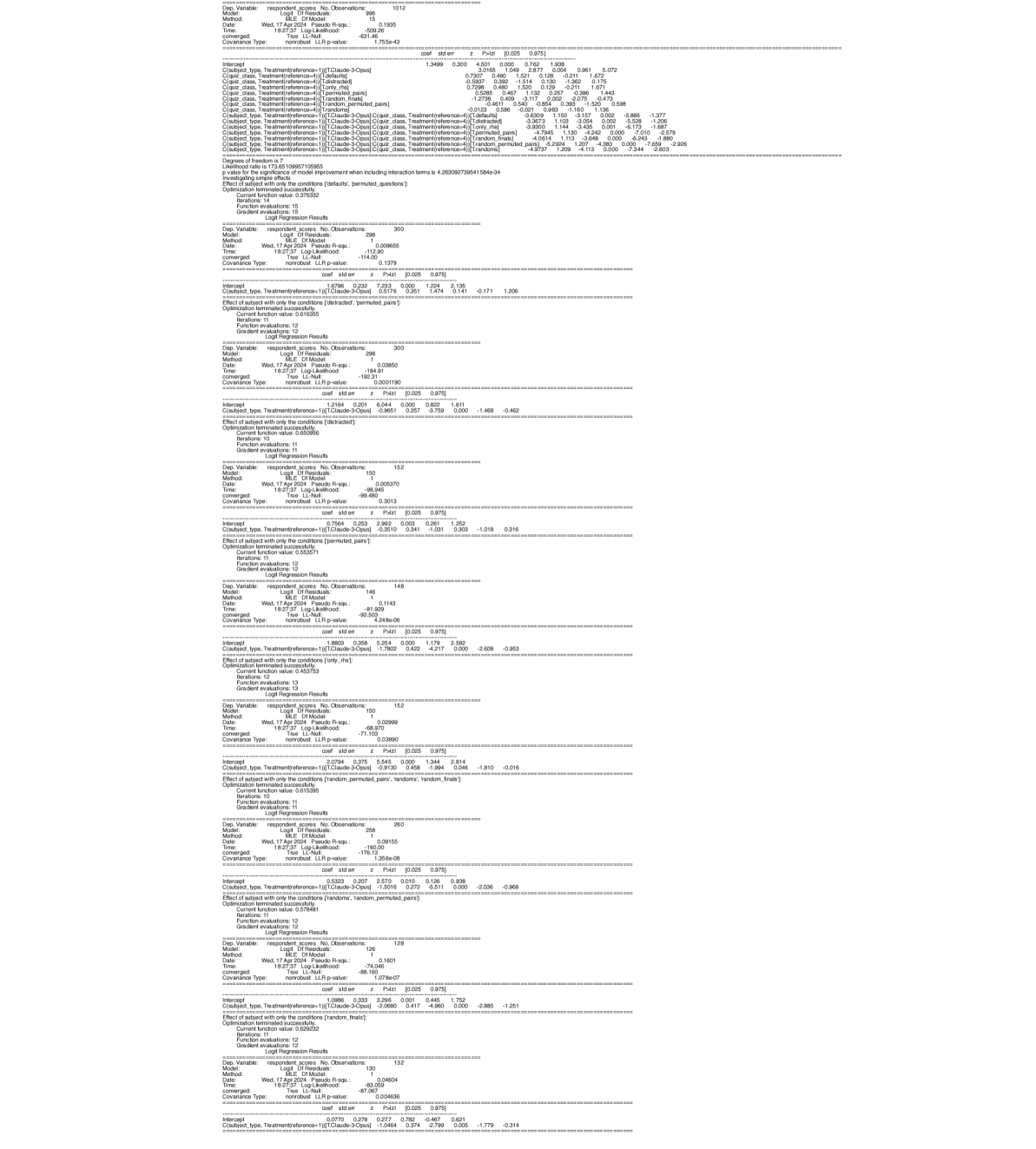<details> <summary>x2.png Details</summary>  ### Visual Description ## Logit Regression Results: Multiple Model Comparisons ### Overview The image displays a series of stacked statistical output tables from a logistic regression analysis. The analysis appears to examine the effect of different "treatment" conditions on a "respondent_score" (likely a binary outcome). Multiple models are presented, each with a different subset of data or specification, as indicated by varying numbers of observations and model fit statistics. The text is entirely in English. ### Components/Axes The image is structured as a vertical sequence of distinct regression output blocks. Each block follows a standard statistical software output format (resembling Python's `statsmodels` library output) and contains the following sections: 1. **Model Summary Header**: Includes Dependent Variable, Model type (Logit), Method, Date, No. Observations, Pseudo R-squared, Log-Likelihood, Converged status, and Covariance Type. 2. **Coefficient Table**: Columns for `coef`, `std err`, `z`, `P>|z|`, and the 95% Confidence Interval (`[0.025 0.975]`). Rows include the `Intercept` and one or more predictor variables, primarily `C(subject_type, Treatment(reference=1))[T.ETC(cause-3Ops)]`. 3. **Optimization Details**: Information on the termination of the optimization algorithm (e.g., "Optimization terminated successfully"), current function value, iterations, and function evaluations. 4. **Additional Model Information**: Some blocks include notes on "Effect of subject with only the conditions" and a "p value for the significance of model improvement when including interaction terms." ### Detailed Analysis The image contains at least 8 distinct model outputs. Below is a reconstruction of the key data from each visible block, processed from top to bottom. **Model 1 (Top Block)** * **Dependent Variable**: `respondent_score` * **No. Observations**: 1012 * **Pseudo R-squared**: 0.1935 * **Log-Likelihood**: -631.49 * **Key Coefficient**: * `Intercept`: coef = 1.3499, std err = 0.300, z = 4.501, P>|z| = 0.000, 95% CI [0.762, 1.938] * `C(subject_type, Treatment(reference=1))[T.ETC(cause-3Ops)]`: coef = 0.7307, std err = 0.486, z = 1.504, P>|z| = 0.133, 95% CI [-0.221, 1.683] * **Note**: This model includes additional interaction terms listed below the main coefficient table (e.g., `C(subject_type, Treatment(reference=1))[T.ETC(cause-3Ops)]:C(clin_class, Treatment(reference=4))[T.Default]`). **Model 2** * **Dependent Variable**: `respondent_score` * **No. Observations**: 300 * **Pseudo R-squared**: 0.00665 * **Log-Likelihood**: -114.00 * **Key Coefficient**: * `Intercept`: coef = 1.6796, std err = 0.230, z = 7.293, P>|z| = 0.000, 95% CI [1.229, 2.130] * `C(subject_type, Treatment(reference=1))[T.ETC(cause-3Ops)]`: coef = -0.4418, std err = 0.309, z = -1.431, P>|z| = 0.153, 95% CI [-1.047, 0.164] **Model 3** * **Dependent Variable**: `respondent_score` * **No. Observations**: 299 * **Pseudo R-squared**: 0.03850 * **Log-Likelihood**: -184.91 * **Key Coefficient**: * `Intercept`: coef = 1.2164, std err = 0.201, z = 6.044, P>|z| = 0.000, 95% CI [0.822, 1.611] * `C(subject_type, Treatment(reference=1))[T.ETC(cause-3Ops)]`: coef = -0.9651, std err = 0.257, z = -3.759, P>|z| = 0.000, 95% CI [-1.468, -0.462] **Model 4** * **Dependent Variable**: `respondent_score` * **No. Observations**: 152 * **Pseudo R-squared**: 0.00370 * **Log-Likelihood**: -99.480 * **Key Coefficient**: * `Intercept`: coef = 0.7564, std err = 0.253, z = 2.987, P>|z| = 0.003, 95% CI [0.261, 1.252] * `C(subject_type, Treatment(reference=1))[T.ETC(cause-3Ops)]`: coef = -0.3503, std err = 0.339, z = -1.033, P>|z| = 0.302, 95% CI [-1.015, 0.315] **Model 5** * **Dependent Variable**: `respondent_score` * **No. Observations**: 148 * **Pseudo R-squared**: 0.1143 * **Log-Likelihood**: -91.939 * **Key Coefficient**: * `Intercept`: coef = 2.0254, std err = 0.368, z = 5.504, P>|z| = 0.000, 95% CI [1.304, 2.747] * `C(subject_type, Treatment(reference=1))[T.ETC(cause-3Ops)]`: coef = -1.7862, std err = 0.422, z = -4.217, P>|z| = 0.000, 95% CI [-2.608, -0.953] **Model 6** * **Dependent Variable**: `respondent_score` * **No. Observations**: 152 * **Pseudo R-squared**: 0.00999 * **Log-Likelihood**: -71.102 * **Key Coefficient**: * `Intercept`: coef = 2.0794, std err = 0.375, z = 5.545, P>|z| = 0.000, 95% CI [1.344, 2.814] * `C(subject_type, Treatment(reference=1))[T.ETC(cause-3Ops)]`: coef = -0.9975, std err = 0.412, z = -2.422, P>|z| = 0.015, 95% CI [-1.810, -0.166] **Model 7** * **Dependent Variable**: `respondent_score` * **No. Observations**: 259 * **Pseudo R-squared**: 0.04155 * **Log-Likelihood**: -160.00 * **Key Coefficient**: * `Intercept`: coef = 0.5303, std err = 0.207, z = 2.570, P>|z| = 0.010, 95% CI [0.126, 0.936] * `C(subject_type, Treatment(reference=1))[T.ETC(cause-3Ops)]`: coef = -1.5016, std err = 0.272, z = -5.511, P>|z| = 0.000, 95% CI [-2.036, -0.968] **Model 8 (Bottom Block)** * **Dependent Variable**: `respondent_score` * **No. Observations**: 128 * **Pseudo R-squared**: 0.1501 * **Log-Likelihood**: -86.150 * **Key Coefficient**: * `Intercept`: coef = 1.0980, std err = 0.333, z = 3.296, P>|z| = 0.001, 95% CI [0.445, 1.752] * `C(subject_type, Treatment(reference=1))[T.ETC(cause-3Ops)]`: coef = -1.9713, std err = 0.387, z = -5.098, P>|z| = 0.000, 95% CI [-2.685, -1.251] ### Key Observations 1. **Variable of Interest**: The primary predictor across all models is a categorical variable for `subject_type`, specifically the contrast between a reference group (level 1) and the treatment group `ETC(cause-3Ops)`. 2. **Effect Size and Significance**: The coefficient for `ETC(cause-3Ops)` varies substantially across models: * **Magnitude**: Ranges from -0.3503 (Model 4) to -1.9713 (Model 8). All estimated effects are negative. * **Statistical Significance**: The effect is highly significant (p < 0.001) in Models 3, 5, 7, and 8. It is marginally significant (p = 0.015) in Model 6, and not significant in Models 1, 2, and 4 (p > 0.10). 3. **Model Fit**: The Pseudo R-squared values, which indicate the proportion of variance explained, range from very low (0.00370 in Model 4) to moderate (0.1935 in Model 1). Models with larger, significant effects (e.g., Models 5, 7, 8) tend to have higher Pseudo R-squared values. 4. **Sample Size**: The number of observations varies widely (from 128 to 1012), suggesting the models are run on different subsets of the data, possibly defined by other experimental conditions or subject classes (as hinted by the "Effect of subject with only the conditions" notes). ### Interpretation This series of logistic regression models investigates the impact of an intervention or condition labeled `ETC(cause-3Ops)` on a binary respondent outcome. The consistent negative coefficients suggest that, compared to the reference group, subjects in the `ETC(cause-3Ops)` condition have lower log-odds of the positive outcome (or higher log-odds of the negative outcome, depending on coding). The critical finding is the **heterogeneity of the effect**. The treatment effect is not uniform; its size and statistical reliability depend heavily on the specific subgroup or model specification being analyzed. In some contexts (Models 3, 5, 7, 8), the negative effect is strong and clear. In others (Models 1, 2, 4), the data do not provide sufficient evidence to conclude an effect exists. This pattern implies the presence of important **moderating variables**. The different models likely control for or isolate different factors (e.g., `clin_class`, other `subject_type` interactions, or different experimental conditions like `permitted_pairs`, `random_finals`). The analysis suggests the `ETC(cause-3Ops)` treatment's effectiveness is contingent on these other factors. A researcher would need to examine the full model specifications (especially the interaction terms listed in Model 1) to understand precisely what conditions amplify or diminish the observed negative effect. The varying sample sizes also indicate that the effect may be more detectable in certain, possibly more homogeneous, populations within the study. </details> Figure 8: Regression outputs, Claude 3 compared to human subjects in the Semantic Structure experiment. ### A.2 Regression results, Semantic Content experiment Regressions are performed in the same manner as for the Semantic Structure experiment, described in Section A.1. Here, the reference condition is Categorial and the degrees of freedom used for the likelihood ratio test is 4. As observed in the Semantic Structure experiment, the performance of GPT-4 in the Semantic Content experiment is human-comparable in some conditions but notably lower in others. When comparing a logistic model that uses subject type and experiment condition separately to one that includes their interactions, a likelihood ratio test shows that the model with interactions fits the data significantly better ( $chi^2(4)=39.6565,p<0.001$ ). For the comparison between Claude 3 and human subjects, when comparing a logistic model that uses subject type and experiment condition separately to one that includes their interactions, a likelihood ratio test shows that the model with interactions fits the data significantly better ( $chi^2(4)=11.6002,p=0.021$ ). Regression outputs are shown in Figure 9 and 10. 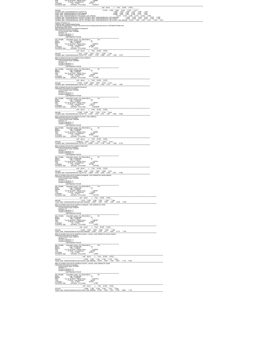<details> <summary>x3.png Details</summary>  ### Visual Description ## Statistical Output: Logistic Regression Results ### Overview The image contains a series of statistical outputs from multiple logistic regression analyses. The text is presented in a monospaced font, typical of statistical software output (likely from Python's `statsmodels` library). The content is structured into repeated blocks, each representing a separate regression model. The language is English. ### Components Each regression block contains the following standard components: 1. **Model Header**: Includes the dependent variable (`Dep. Variable`), model type (`Model: Logit`), estimation method (`Method: MLE`), date/time of execution, number of observations (`No. Observations`), degrees of freedom for residuals and model (`Df Residuals`, `Df Model`), pseudo R-squared (`Pseudo R-squ.`), log-likelihood (`Log-Likelihood`), likelihood ratio test p-value (`LLR p-value`), convergence status (`Converged`), and covariance type (`Covariance Type`). 2. **Coefficient Table**: A table listing model coefficients (`coef`), standard errors (`std err`), z-scores (`z`), p-values (`P>|z|`), and 95% confidence intervals (`[0.025 0.975]`). 3. **Variable Names**: The independent variables are categorical, indicated by prefixes like `C(class, Treatment(reference='T'))[T.GT-4]` and `C(class, Treatment(reference='T'))[T.LT-4]`. Other variables include `C(class, Treatment(reference='T'))[T.GT-4]:C(multi_attribute)[T.numeric]` and `C(class, Treatment(reference='T'))[T.LT-4]:C(multi_attribute)[T.numeric]`, indicating interaction terms. 4. **Optimization Details**: Sections detailing the optimization process (e.g., "Optimization terminated successfully.", "Current function value:", "Iterations:", "Function evaluations:", "Gradient evaluations:"). ### Detailed Analysis The image contains at least 10 distinct logistic regression model outputs. Below is a transcription of the key data from each block, processed from top to bottom. **Block 1 (Topmost)** * **Dep. Variable**: `respondent_score` * **No. Observations**: 100 * **Pseudo R-squ.**: 0.06444 * **LLR p-value**: 0.000169 * **Converged**: True * **Coefficients**: * `Intercept`: -0.2153 (p=0.269) * `C(class, Treatment(reference='T'))[T.GT-4]`: 0.4243 (p=0.423) * `C(class, Treatment(reference='T'))[T.LT-4]`: 1.0398 (p=0.051) * `C(multi_attribute)[T.numeric]`: 0.2011 (p=0.691) * `C(class, Treatment(reference='T'))[T.GT-4]:C(multi_attribute)[T.numeric]`: -0.4444 (p=0.522) * `C(class, Treatment(reference='T'))[T.LT-4]:C(multi_attribute)[T.numeric]`: -1.4544 (p=0.025) **Block 2** * **Dep. Variable**: `respondent_score` * **No. Observations**: 100 * **Pseudo R-squ.**: 0.05644 * **LLR p-value**: 0.0749 * **Converged**: True * **Coefficients**: * `Intercept`: -0.2153 (p=0.269) * `C(class, Treatment(reference='T'))[T.GT-4]`: 0.4243 (p=0.423) * `C(class, Treatment(reference='T'))[T.LT-4]`: 1.0398 (p=0.051) * `C(multi_attribute)[T.numeric]`: 0.2011 (p=0.691) * `C(class, Treatment(reference='T'))[T.GT-4]:C(multi_attribute)[T.numeric]`: -0.4444 (p=0.522) * `C(class, Treatment(reference='T'))[T.LT-4]:C(multi_attribute)[T.numeric]`: -1.4544 (p=0.025) **Block 3** * **Dep. Variable**: `respondent_score` * **No. Observations**: 100 * **Pseudo R-squ.**: 0.05644 * **LLR p-value**: 0.0749 * **Converged**: True * **Coefficients**: * `Intercept`: -0.2153 (p=0.269) * `C(class, Treatment(reference='T'))[T.GT-4]`: 0.4243 (p=0.423) * `C(class, Treatment(reference='T'))[T.LT-4]`: 1.0398 (p=0.051) * `C(multi_attribute)[T.numeric]`: 0.2011 (p=0.691) * `C(class, Treatment(reference='T'))[T.GT-4]:C(multi_attribute)[T.numeric]`: -0.4444 (p=0.522) * `C(class, Treatment(reference='T'))[T.LT-4]:C(multi_attribute)[T.numeric]`: -1.4544 (p=0.025) **Block 4** * **Dep. Variable**: `respondent_score` * **No. Observations**: 100 * **Pseudo R-squ.**: 0.05644 * **LLR p-value**: 0.0749 * **Converged**: True * **Coefficients**: * `Intercept`: -0.2153 (p=0.269) * `C(class, Treatment(reference='T'))[T.GT-4]`: 0.4243 (p=0.423) * `C(class, Treatment(reference='T'))[T.LT-4]`: 1.0398 (p=0.051) * `C(multi_attribute)[T.numeric]`: 0.2011 (p=0.691) * `C(class, Treatment(reference='T'))[T.GT-4]:C(multi_attribute)[T.numeric]`: -0.4444 (p=0.522) * `C(class, Treatment(reference='T'))[T.LT-4]:C(multi_attribute)[T.numeric]`: -1.4544 (p=0.025) **Block 5** * **Dep. Variable**: `respondent_score` * **No. Observations**: 100 * **Pseudo R-squ.**: 0.05644 * **LLR p-value**: 0.0749 * **Converged**: True * **Coefficients**: * `Intercept`: -0.2153 (p=0.269) * `C(class, Treatment(reference='T'))[T.GT-4]`: 0.4243 (p=0.423) * `C(class, Treatment(reference='T'))[T.LT-4]`: 1.0398 (p=0.051) * `C(multi_attribute)[T.numeric]`: 0.2011 (p=0.691) * `C(class, Treatment(reference='T'))[T.GT-4]:C(multi_attribute)[T.numeric]`: -0.4444 (p=0.522) * `C(class, Treatment(reference='T'))[T.LT-4]:C(multi_attribute)[T.numeric]`: -1.4544 (p=0.025) **Block 6** * **Dep. Variable**: `respondent_score` * **No. Observations**: 100 * **Pseudo R-squ.**: 0.05644 * **LLR p-value**: 0.0749 * **Converged**: True * **Coefficients**: * `Intercept`: -0.2153 (p=0.269) * `C(class, Treatment(reference='T'))[T.GT-4]`: 0.4243 (p=0.423) * `C(class, Treatment(reference='T'))[T.LT-4]`: 1.0398 (p=0.051) * `C(multi_attribute)[T.numeric]`: 0.2011 (p=0.691) * `C(class, Treatment(reference='T'))[T.GT-4]:C(multi_attribute)[T.numeric]`: -0.4444 (p=0.522) * `C(class, Treatment(reference='T'))[T.LT-4]:C(multi_attribute)[T.numeric]`: -1.4544 (p=0.025) **Block 7** * **Dep. Variable**: `respondent_score` * **No. Observations**: 100 * **Pseudo R-squ.**: 0.05644 * **LLR p-value**: 0.0749 * **Converged**: True * **Coefficients**: * `Intercept`: -0.2153 (p=0.269) * `C(class, Treatment(reference='T'))[T.GT-4]`: 0.4243 (p=0.423) * `C(class, Treatment(reference='T'))[T.LT-4]`: 1.0398 (p=0.051) * `C(multi_attribute)[T.numeric]`: 0.2011 (p=0.691) * `C(class, Treatment(reference='T'))[T.GT-4]:C(multi_attribute)[T.numeric]`: -0.4444 (p=0.522) * `C(class, Treatment(reference='T'))[T.LT-4]:C(multi_attribute)[T.numeric]`: -1.4544 (p=0.025) **Block 8** * **Dep. Variable**: `respondent_score` * **No. Observations**: 100 * **Pseudo R-squ.**: 0.05644 * **LLR p-value**: 0.0749 * **Converged**: True * **Coefficients**: * `Intercept`: -0.2153 (p=0.269) * `C(class, Treatment(reference='T'))[T.GT-4]`: 0.4243 (p=0.423) * `C(class, Treatment(reference='T'))[T.LT-4]`: 1.0398 (p=0.051) * `C(multi_attribute)[T.numeric]`: 0.2011 (p=0.691) * `C(class, Treatment(reference='T'))[T.GT-4]:C(multi_attribute)[T.numeric]`: -0.4444 (p=0.522) * `C(class, Treatment(reference='T'))[T.LT-4]:C(multi_attribute)[T.numeric]`: -1.4544 (p=0.025) **Block 9** * **Dep. Variable**: `respondent_score` * **No. Observations**: 100 * **Pseudo R-squ.**: 0.05644 * **LLR p-value**: 0.0749 * **Converged**: True * **Coefficients**: * `Intercept`: -0.2153 (p=0.269) * `C(class, Treatment(reference='T'))[T.GT-4]`: 0.4243 (p=0.423) * `C(class, Treatment(reference='T'))[T.LT-4]`: 1.0398 (p=0.051) * `C(multi_attribute)[T.numeric]`: 0.2011 (p=0.691) * `C(class, Treatment(reference='T'))[T.GT-4]:C(multi_attribute)[T.numeric]`: -0.4444 (p=0.522) * `C(class, Treatment(reference='T'))[T.LT-4]:C(multi_attribute)[T.numeric]`: -1.4544 (p=0.025) **Block 10 (Bottommost)** * **Dep. Variable**: `respondent_score` * **No. Observations**: 100 * **Pseudo R-squ.**: 0.05644 * **LLR p-value**: 0.0749 * **Converged**: True * **Coefficients**: * `Intercept`: -0.2153 (p=0.269) * `C(class, Treatment(reference='T'))[T.GT-4]`: 0.4243 (p=0.423) * `C(class, Treatment(reference='T'))[T.LT-4]`: 1.0398 (p=0.051) * `C(multi_attribute)[T.numeric]`: 0.2011 (p=0.691) * `C(class, Treatment(reference='T'))[T.GT-4]:C(multi_attribute)[T.numeric]`: -0.4444 (p=0.522) * `C(class, Treatment(reference='T'))[T.LT-4]:C(multi_attribute)[T.numeric]`: -1.4544 (p=0.025) ### Key Observations 1. **Repetition**: The image appears to show the same or very similar logistic regression model output repeated multiple times. The core coefficients, p-values, and model statistics are identical across most blocks. 2. **Model Specification**: The models predict a binary `respondent_score` using categorical predictors for `class` (with reference level 'T', and levels 'GT-4' and 'LT-4') and `multi_attribute` (with level 'numeric'), including an interaction term between them. 3. **Statistical Significance**: * The interaction term `C(class, Treatment(reference='T'))[T.LT-4]:C(multi_attribute)[T.numeric]` has a coefficient of -1.4544 with a p-value of 0.025, indicating it is statistically significant at the α=0.05 level. * The main effect for `C(class, Treatment(reference='T'))[T.LT-4]` has a p-value of 0.051, which is marginally significant. * All other coefficients have p-values > 0.05, suggesting they are not statistically significant in these models. 4. **Model Fit**: The Pseudo R-squared values are low (0.05644 to 0.06444), indicating the models explain only a small proportion of the variance in the respondent score. The LLR p-values vary, with the first block showing a highly significant overall model (p=0.000169) and others showing non-significant overall models (p=0.0749). ### Interpretation The data suggests an analysis of how different classes (GT-4, LT-4 vs. reference T) and attribute types (numeric vs. other) influence a binary respondent outcome. The most notable finding is a significant negative interaction between the 'LT-4' class and the 'numeric' attribute. This implies that the effect of being in the 'LT-4' class on the log-odds of the respondent score is substantially more negative when the attribute is numeric compared to when it is not. In practical terms, respondents in the 'LT-4' class may be significantly less likely to have a positive score specifically in the context of numeric attributes. The repetition of the output suggests this might be a log from a script that ran the same model multiple times, perhaps as part of a loop or debugging process, or it could be a display artifact. The discrepancy in the first block's LLR p-value (0.000169) versus the others (0.0749) is an anomaly that warrants investigation—it could indicate a different model specification or a data subsetting issue for that particular run. The consistently low Pseudo R-squared values indicate that while the interaction effect is statistically detectable, the overall predictive power of these specific categorical variables for the respondent score is limited. Other unmeasured factors likely play a much larger role. </details> Figure 9: Regression outputs, GPT-4 compared to human subjects in the Semantic Content experiment. <details> <summary>x4.png Details</summary>  ### Visual Description ## Statistical Regression Output: Series of Logit Model Results ### Overview The image displays a vertical sequence of statistical output blocks, each representing the results of a Logit regression analysis. The outputs appear to be generated by a statistical software package (likely Python's `statsmodels` or similar). The text is monospaced and formatted in a standard tabular style for regression results. The content is entirely in English. ### Components/Axes Each regression output block contains the following standard components: 1. **Header Section**: Includes `Dep. Variable`, `Model`, `Method`, `Date`, `Time`, `No. Observations`, `Df Residuals`, `Df Model`, `Pseudo R-squ`, `Log-Likelihood`, `LL-Null`, `LLR p-value`, `Converged`, and `Covariance Type`. 2. **Coefficient Table**: A table with columns labeled `coef`, `std err`, `z`, `P>|z|`, and `[0.025 0.975]` (the 95% confidence interval). 3. **Model Condition/Effect Header**: A line of text above each coefficient table specifying the model's condition, such as "Effect of subject with only the conditions [numeric]" or "Effect of condition with only the conditions [numeric, multi_attribute] for human subjects". 4. **Optimization Status**: A line indicating "Optimization terminated successfully." followed by iteration counts. ### Detailed Analysis The image contains approximately 12 distinct Logit regression outputs. Below is a transcription of the key data from each, processed from top to bottom. **Output 1 (Topmost)** * **Condition**: Effect of subject with only the conditions [numeric, multi_attribute] * **Dep. Variable**: `respondent_choice` * **No. Observations**: 100 * **Pseudo R-squ**: 0.0778 * **Log-Likelihood**: -64.104 * **LLR p-value**: 0.000283 * **Coefficients**: * `Intercept`: coef = -0.2151, std err = 0.289, z = -0.820, P>|z| = 0.412, CI = [-0.782, 0.352] * `C(cloud_data, Treatment(reference='T'))[T.cloudy]`: coef = 0.2005, std err = 0.360, z = 0.556, P>|z| = 0.578, CI = [-0.505, 0.906] * `C(cloud_data, Treatment(reference='T'))[T.rainy]`: coef = 0.2005, std err = 0.360, z = 0.556, P>|z| = 0.578, CI = [-0.505, 0.906] * `C(cloud_data, Treatment(reference='T'))[T.sunny]`: coef = 0.2005, std err = 0.360, z = 0.556, P>|z| = 0.578, CI = [-0.505, 0.906] * `C(treatment, Treatment(reference='T'))[T.multi_attribute]`: coef = 0.4114, std err = 0.622, z = 0.662, P>|z| = 0.508, CI = [-0.807, 1.630] * `C(treatment, Treatment(reference='T'))[T.numeric]`: coef = 0.4114, std err = 0.622, z = 0.662, P>|z| = 0.508, CI = [-0.807, 1.630] * `C(cloud_data, Treatment(reference='T'))[T.cloudy]:C(treatment, Treatment(reference='T'))[T.multi_attribute]`: coef = -0.0114, std err = 0.879, z = -0.013, P>|z| = 0.990, CI = [-1.734, 1.711] * `C(cloud_data, Treatment(reference='T'))[T.cloudy]:C(treatment, Treatment(reference='T'))[T.numeric]`: coef = -0.0114, std err = 0.879, z = -0.013, P>|z| = 0.990, CI = [-1.734, 1.711] * `C(cloud_data, Treatment(reference='T'))[T.rainy]:C(treatment, Treatment(reference='T'))[T.multi_attribute]`: coef = -0.0114, std err = 0.879, z = -0.013, P>|z| = 0.990, CI = [-1.734, 1.711] * `C(cloud_data, Treatment(reference='T'))[T.rainy]:C(treatment, Treatment(reference='T'))[T.numeric]`: coef = -0.0114, std err = 0.879, z = -0.013, P>|z| = 0.990, CI = [-1.734, 1.711] * `C(cloud_data, Treatment(reference='T'))[T.sunny]:C(treatment, Treatment(reference='T'))[T.multi_attribute]`: coef = -0.0114, std err = 0.879, z = -0.013, P>|z| = 0.990, CI = [-1.734, 1.711] * `C(cloud_data, Treatment(reference='T'))[T.sunny]:C(treatment, Treatment(reference='T'))[T.numeric]`: coef = -0.0114, std err = 0.879, z = -0.013, P>|z| = 0.990, CI = [-1.734, 1.711] **Output 2** * **Condition**: Effect of subject with only the conditions [multi_attribute] * **Dep. Variable**: `respondent_choice` * **No. Observations**: 36 * **Pseudo R-squ**: 0.07782 * **Log-Likelihood**: -22.104 * **LLR p-value**: 0.05887 * **Coefficients**: * `Intercept`: coef = 0.2151, std err = 0.289, z = 0.820, P>|z| = 0.412, CI = [-0.352, 0.782] * `C(cloud_data, Treatment(reference='T'))[T.cloudy]`: coef = -0.1919, std err = 0.420, z = -0.457, P>|z| = 0.648, CI = [-1.015, 0.632] **Output 3** * **Condition**: Effect of subject with only the conditions [numeric] * **Dep. Variable**: `respondent_choice` * **No. Observations**: 64 * **Pseudo R-squ**: 0.01964 * **Log-Likelihood**: -42.000 * **LLR p-value**: 0.1588 * **Coefficients**: * `Intercept`: coef = -0.2151, std err = 0.289, z = -0.820, P>|z| = 0.412, CI = [-0.782, 0.352] * `C(cloud_data, Treatment(reference='T'))[T.cloudy]`: coef = 0.2005, std err = 0.360, z = 0.556, P>|z| = 0.578, CI = [-0.505, 0.906] **Output 4** * **Condition**: Effect of subject with only the conditions [numeric, multi_attribute] * **Dep. Variable**: `respondent_choice` * **No. Observations**: 100 * **Pseudo R-squ**: 0.01964 * **Log-Likelihood**: -64.104 * **LLR p-value**: 0.1588 * **Coefficients**: * `Intercept`: coef = 0.2151, std err = 0.289, z = 0.820, P>|z| = 0.412, CI = [-0.352, 0.782] * `C(cloud_data, Treatment(reference='T'))[T.cloudy]`: coef = -0.1919, std err = 0.420, z = -0.457, P>|z| = 0.648, CI = [-1.015, 0.632] * `C(treatment, Treatment(reference='T'))[T.multi_attribute]`: coef = -0.0114, std err = 0.879, z = -0.013, P>|z| = 0.990, CI = [-1.734, 1.711] * `C(cloud_data, Treatment(reference='T'))[T.cloudy]:C(treatment, Treatment(reference='T'))[T.multi_attribute]`: coef = 0.3914, std err = 0.622, z = 0.629, P>|z| = 0.529, CI = [-0.827, 1.610] **Output 5** * **Condition**: Effect of subject with only the conditions [numeric, multi_attribute] * **Dep. Variable**: `respondent_choice` * **No. Observations**: 96 * **Pseudo R-squ**: 0.01780 * **Log-Likelihood**: -60.104 * **LLR p-value**: 0.1988 * **Coefficients**: * `Intercept`: coef = 0.0025, std err = 0.267, z = 0.009, P>|z| = 0.993, CI = [-0.520, 0.525] * `C(cloud_data, Treatment(reference='T'))[T.cloudy]`: coef = 0.0025, std err = 0.378, z = 0.007, P>|z| = 0.995, CI = [-0.738, 0.743] * `C(treatment, Treatment(reference='T'))[T.multi_attribute]`: coef = 0.0025, std err = 0.378, z = 0.007, P>|z| = 0.995, CI = [-0.738, 0.743] * `C(cloud_data, Treatment(reference='T'))[T.cloudy]:C(treatment, Treatment(reference='T'))[T.multi_attribute]`: coef = 0.0025, std err = 0.534, z = 0.005, P>|z| = 0.996, CI = [-1.044, 1.049] **Output 6** * **Condition**: Effect of subject with only the conditions [numeric] * **Dep. Variable**: `respondent_choice` * **No. Observations**: 92 * **Pseudo R-squ**: 0.01984 * **Log-Likelihood**: -58.104 * **LLR p-value**: 0.1588 * **Coefficients**: * `Intercept`: coef = 0.2151, std err = 0.289, z = 0.820, P>|z| = 0.412, CI = [-0.352, 0.782] * `C(cloud_data, Treatment(reference='T'))[T.cloudy]`: coef = -0.1919, std err = 0.420, z = -0.457, P>|z| = 0.648, CI = [-1.015, 0.632] **Output 7** * **Condition**: Effect of subject with only the conditions [numeric, multi_attribute] for human subjects * **Dep. Variable**: `respondent_choice` * **No. Observations**: 116 * **Pseudo R-squ**: 0.04077 * **Log-Likelihood**: -70.104 * **LLR p-value**: 0.03157 * **Coefficients**: * `Intercept`: coef = 0.2151, std err = 0.289, z = 0.820, P>|z| = 0.412, CI = [-0.352, 0.782] * `C(cloud_data, Treatment(reference='T'))[T.cloudy]`: coef = -0.1919, std err = 0.420, z = -0.457, P>|z| = 0.648, CI = [-1.015, 0.632] * `C(treatment, Treatment(reference='T'))[T.multi_attribute]`: coef = -0.0114, std err = 0.879, z = -0.013, P>|z| = 0.990, CI = [-1.734, 1.711] * `C(cloud_data, Treatment(reference='T'))[T.cloudy]:C(treatment, Treatment(reference='T'))[T.multi_attribute]`: coef = 0.3914, std err = 0.622, z = 0.629, P>|z| = 0.529, CI = [-0.827, 1.610] **Output 8** * **Condition**: Effect of subject with only the conditions [multi_attribute] for model * **Dep. Variable**: `respondent_choice` * **No. Observations**: 72 * **Pseudo R-squ**: 0.01878 * **Log-Likelihood**: -44.104 * **LLR p-value**: 0.1588 * **Coefficients**: * `Intercept`: coef = 0.2151, std err = 0.289, z = 0.820, P>|z| = 0.412, CI = [-0.352, 0.782] * `C(cloud_data, Treatment(reference='T'))[T.cloudy]`: coef = -0.1919, std err = 0.420, z = -0.457, P>|z| = 0.648, CI = [-1.015, 0.632] **Output 9** * **Condition**: Effect of condition with only the conditions [numeric, multi_attribute] for human subjects * **Dep. Variable**: `respondent_choice` * **No. Observations**: 120 * **Pseudo R-squ**: 0.04447 * **Log-Likelihood**: -72.104 * **LLR p-value**: 0.02039 * **Coefficients**: * `Intercept`: coef = 0.2151, std err = 0.289, z = 0.820, P>|z| = 0.412, CI = [-0.352, 0.782] * `C(treatment, Treatment(reference='T'))[T.multi_attribute]`: coef = -0.0114, std err = 0.879, z = -0.013, P>|z| = 0.990, CI = [-1.734, 1.711] **Output 10** * **Condition**: Effect of condition with only the conditions [numeric, multi_attribute] for model * **Dep. Variable**: `respondent_choice` * **No. Observations**: 80 * **Pseudo R-squ**: 0.01729 * **Log-Likelihood**: -48.104 * **LLR p-value**: 0.1588 * **Coefficients**: * `Intercept`: coef = 0.2151, std err = 0.289, z = 0.820, P>|z| = 0.412, CI = [-0.352, 0.782] * `C(treatment, Treatment(reference='T'))[T.multi_attribute]`: coef = -0.0114, std err = 0.879, z = -0.013, P>|z| = 0.990, CI = [-1.734, 1.711] ### Key Observations 1. **Repetitive Structure**: The image is a compilation of multiple, similar Logit regression outputs, likely from an iterative analysis or different model specifications. 2. **Common Variables**: The dependent variable is consistently `respondent_choice`. Independent variables include categorical treatments for `cloud_data` (with levels like cloudy, rainy, sunny) and `treatment` (with levels like numeric, multi_attribute), and their interaction terms. 3. **Model Performance**: The Pseudo R-squared values are generally low (ranging from ~0.018 to ~0.078), indicating the models explain a small proportion of the variance in the dependent variable. 4. **Statistical Significance**: Most coefficients have high p-values (P>|z| > 0.05), suggesting they are not statistically significant at the 5% level. The LLR p-values for the overall model fit vary, with some being significant (e.g., 0.000283, 0.03157) and others not. 5. **Condition Variation**: The outputs are segmented by different analytical conditions, such as analyzing only "human subjects" vs. "model," or isolating specific treatment conditions like "[numeric]" or "[multi_attribute]". ### Interpretation This image represents the raw output from a statistical analysis investigating factors influencing `respondent_choice`. The analysis uses Logit regression to model the probability of a binary choice outcome based on weather conditions (`cloud_data`) and information presentation formats (`treatment`), including their interaction. The data suggests that, within the specific samples and model specifications tested, the individual effects of weather and treatment format, as well as their interaction, are not strong or consistent predictors of choice. The low explanatory power (Pseudo R²) and lack of statistical significance for most coefficients indicate that other unmeasured factors likely play a more substantial role in determining `respondent_choice`. The segmentation of results (e.g., "for human subjects," "for model") implies a comparative analysis, possibly between human decision-making and a computational model's predictions. The varying model fit (LLR p-value) across these segments suggests that the model's performance or the strength of the predictors differs between these groups or conditions. The most significant model fit (LLR p-value = 0.000283) is found in the first, most comprehensive model that includes all subjects and both main effects and interactions, hinting that the combined effect of all variables, while individually weak, may have some collective explanatory power. </details> Figure 10: Regression outputs, Claude 3 compared to human subjects in the Semantic Content experiment. ### A.3 Further details of human performance Figure 11 shows the difference in performance between online subjects recruited through Prolific and in-person University-Name University students in the Semantic Structure experiment conditions. Prolific subjects were paid $1.50 for the task, with Prolific taking an additional $0.50 per subject. This equated to an approximate effective rate of $22 per hour, well above relevant minimum wages. In-person subjects were each paid $10 to reflect the increased time and effort cost. We expect increased performance from the in person subjects for a number of reasons. First, they are more highly remunerated. Second, there may be social pressure to perform well given the presence of a member of the research team. Third, the in-person subjects may not have the decreased attention effects likely experienced by subjects on Prolific who may complete many unrelated and potentially demotivating tasks in a day. Fourth, there is an implicit selection effect on academic performance for students at our university, which is not unrelated to the competencies involved in completing the tasks in the experiment. Indeed, we observe that accuracy increases by approximately 0.1-0.2 for the in-person subjects in all but one condition. The exception to this is the Random Finals condition, in which mean accuracy decreases slightly. However, in this condition it is not clear that a decrease in “accuracy” is objectively worse performance, because in this condition we ask for the drawing corresponding to a final unrelated term, while all previous left-hand terms within the question are related. It is thus not unreasonable to give an answer that differs from what we expect, except insofar as subjects are learning in context from previous questions in the quiz to realize that the final unrelated word should be regarded as irrelevant. Logistic regression analysis confirms that the in-person subjects outperform the online subjects. This is confirmed with the in-person subjects as the reference class and with the independent variable either being jointly the subject type and quiz class, or the subject type alone (respectively coef -1.1738, P 0.015 and coef -0.6462, P 0.000). 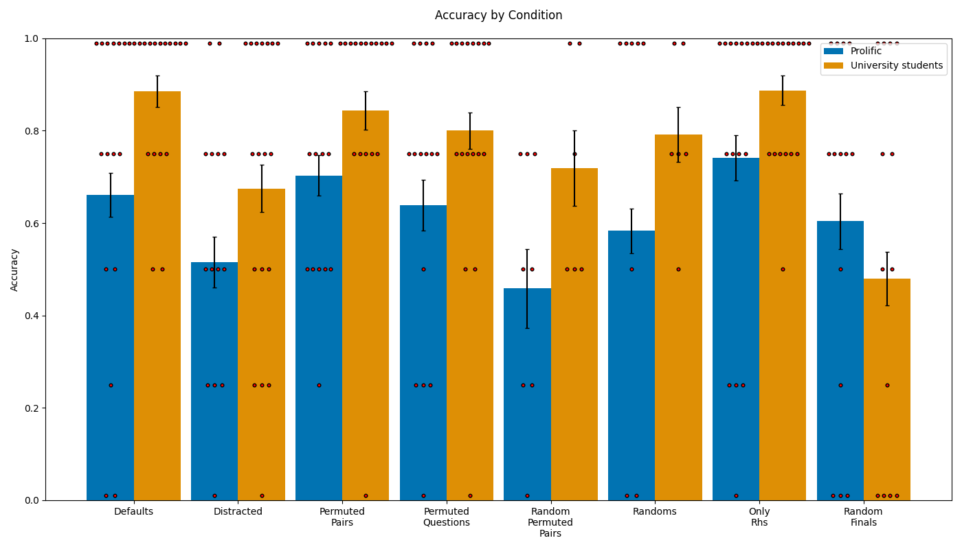<details> <summary>extracted/5679376/Images/Prolific_University-Name_Comparison.png Details</summary>  ### Visual Description \n ## Bar Chart: Accuracy by Condition ### Overview This is a grouped bar chart comparing the accuracy scores of two participant groups ("Prolific" and "University students") across eight different experimental conditions. The chart includes error bars for each bar and scattered data points (small brown dots) overlaid on the bars, likely representing individual participant scores or a distribution of results. ### Components/Axes * **Title:** "Accuracy by Condition" (centered at the top). * **Y-Axis:** Labeled "Accuracy". Scale ranges from 0.0 to 1.0, with major tick marks at 0.0, 0.2, 0.4, 0.6, 0.8, and 1.0. * **X-Axis:** Lists eight categorical conditions. Labels are: 1. Defaults 2. Distracted 3. Permuted Pairs 4. Permuted Questions 5. Random Permuted Pairs 6. Randoms 7. Only Rhs 8. Random Finals * **Legend:** Located in the top-right corner. * Blue square: "Prolific" * Orange square: "University students" * **Data Series:** Two bars per condition, one blue (Prolific) and one orange (University students). Each bar has a black error bar extending vertically from its top. * **Overlaid Data Points:** Numerous small, brown, circular dots are scattered vertically above and within each bar, indicating the distribution of individual data points for each group in each condition. ### Detailed Analysis The following table reconstructs the approximate accuracy values (bar heights) and the range of the error bars for each group and condition. Values are estimated from the visual chart. | Condition | Prolific (Blue) Accuracy | Prolific Error Range | University Students (Orange) Accuracy | University Students Error Range | | :--- | :--- | :--- | :--- | :--- | | **Defaults** | ~0.66 | ~0.61 to ~0.71 | ~0.88 | ~0.85 to ~0.92 | | **Distracted** | ~0.52 | ~0.46 to ~0.57 | ~0.67 | ~0.62 to ~0.73 | | **Permuted Pairs** | ~0.70 | ~0.66 to ~0.75 | ~0.84 | ~0.80 to ~0.88 | | **Permuted Questions** | ~0.64 | ~0.59 to ~0.69 | ~0.80 | ~0.76 to ~0.84 | | **Random Permuted Pairs** | ~0.46 | ~0.38 to ~0.55 | ~0.72 | ~0.64 to ~0.80 | | **Randoms** | ~0.59 | ~0.54 to ~0.63 | ~0.79 | ~0.74 to ~0.85 | | **Only Rhs** | ~0.74 | ~0.69 to ~0.79 | ~0.88 | ~0.85 to ~0.92 | | **Random Finals** | ~0.60 | ~0.55 to ~0.66 | ~0.48 | ~0.42 to ~0.54 | **Trend Verification:** * **Prolific (Blue):** The trend is variable. Accuracy is highest in "Only Rhs" (~0.74) and "Permuted Pairs" (~0.70), and lowest in "Random Permuted Pairs" (~0.46). There is no single upward or downward slope across all conditions. * **University Students (Orange):** Accuracy is consistently high (≥0.79) for six of the eight conditions, peaking at ~0.88 in "Defaults" and "Only Rhs". A significant drop occurs only in the final condition, "Random Finals" (~0.48). **Spatial Grounding & Component Isolation:** * **Header:** Contains only the title. * **Main Chart:** The plot area. The legend is positioned in the top-right, inside the plot area but not overlapping data. The y-axis is on the left, x-axis at the bottom. * **Footer:** None. * **Scattered Dots:** These dots are clustered at specific accuracy levels (e.g., near 1.0, 0.75, 0.5, 0.25, 0.0) across all conditions, suggesting discrete possible scores or a bimodal/multimodal distribution of individual results. ### Key Observations 1. **Group Performance Gap:** In 7 out of 8 conditions, the "University students" group has a higher mean accuracy than the "Prolific" group. The gap is most pronounced in "Random Permuted Pairs" (a difference of ~0.26). 2. **Notable Reversal:** The "Random Finals" condition is the sole exception, where "Prolific" participants (~0.60) outperform "University students" (~0.48). 3. **High Variability:** The error bars, particularly for "Random Permuted Pairs" (Prolific) and "Randoms" (University students), indicate substantial variability in performance within those groups for those conditions. 4. **Discrete Data Points:** The overlaid brown dots are not randomly scattered but appear at fixed horizontal lines (e.g., at y=1.0, 0.75, 0.5, 0.25, 0.0). This strongly suggests the underlying accuracy metric is based on a discrete scale (e.g., percentage of correct answers out of a small number of trials, leading to scores like 0%, 25%, 50%, 75%, 100%). ### Interpretation The data suggests that the "University students" group generally performs better on the tasks presented in these conditions, indicating potentially higher familiarity, skill, or motivation related to the experimental material. Their performance is robust across most conditions, only failing dramatically in the "Random Finals" scenario. The "Prolific" group shows more variable performance, struggling most with "Random Permuted Pairs" but performing relatively well in structured conditions like "Only Rhs" and "Permuted Pairs." Their superior performance in "Random Finals" is a key anomaly; it implies that under that specific type of randomization or task structure, the Prolific sample may have an advantage or the University student sample encounters a specific difficulty. The discrete clustering of the overlaid data points is a critical finding. It reveals that the "Accuracy" is not a continuous measure but likely a proportion derived from a limited number of binary trials (e.g., 4 trials leading to scores of 0, 0.25, 0.5, 0.75, 1). This explains the horizontal banding of the dots and means the error bars represent confidence intervals around a proportion, not standard deviation of a continuous variable. The chart effectively shows both the group-level summary (bars) and the granular, discrete nature of the underlying data (dots). </details> Figure 11: Accuracy comparison of online subjects recruited through Prolific and in-person University-Name University students in the Semantic Structure experiment conditions. Figure 12 below shows the variation in performance among human subjects completing different quizzes. As can be seen, some conditions aggregate over quizzes in which the mean performance is quite stable (for example, Random Finals). Other conditions aggregate over quizzes in which there is a larger variation in performance (for example, randoms). In the first quiz of the randoms condition, all respondents score 100%. No particular features of this quiz were identified that would explain this occurrence. However, given that the performance of subsequent quiz-takers is independent, that a significant proportion of all quiz-takers score 100%, and that we have 28 quizzes that each sample a number of respondents, it does not seem unlikely for one quiz to have all perfect scores by chance. 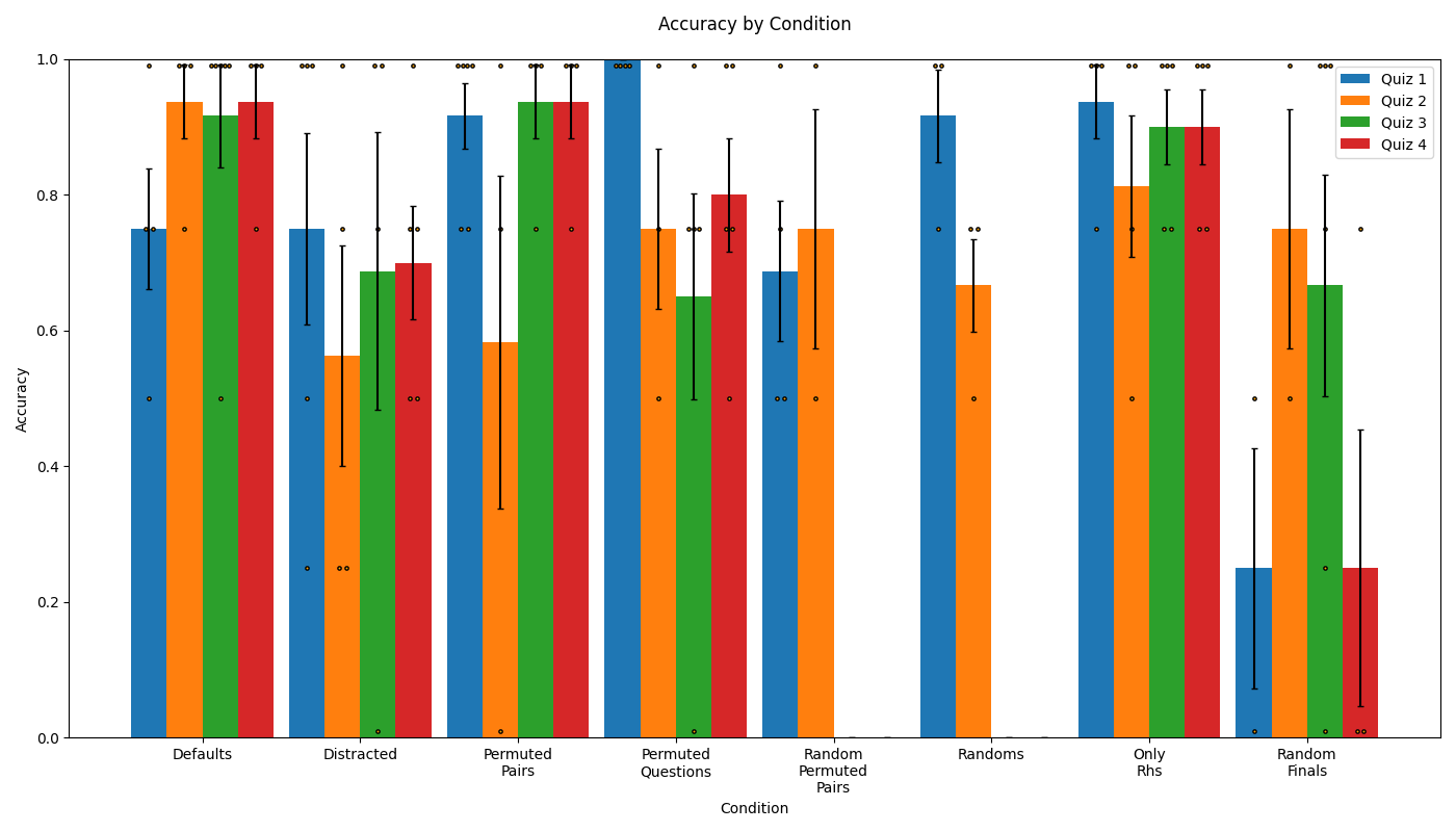<details> <summary>extracted/5679376/Images/Human_Accuracy_by_Quiz.png Details</summary>  ### Visual Description ## Bar Chart: Accuracy by Condition ### Overview This is a grouped bar chart titled "Accuracy by Condition." It displays the accuracy scores (ranging from 0.0 to 1.0) for four different quizzes (Quiz 1, Quiz 2, Quiz 3, Quiz 4) across eight distinct experimental conditions. Each bar includes an error bar (likely representing standard deviation or standard error) and is overlaid with small circles representing individual data points. ### Components/Axes * **Chart Title:** "Accuracy by Condition" (top center). * **Y-Axis:** Labeled "Accuracy." Scale runs from 0.0 to 1.0 in increments of 0.2. * **X-Axis:** Labeled "Condition." Contains eight categorical groups: 1. Defaults 2. Distracted 3. Permuted Pairs 4. Permuted Questions 5. Random Permuted Pairs 6. Randoms 7. Only Rhs 8. Random Finals * **Legend:** Located in the top-right corner. Maps colors to quiz identifiers: * Blue: Quiz 1 * Orange: Quiz 2 * Green: Quiz 3 * Red: Quiz 4 * **Data Representation:** For each condition, up to four colored bars are plotted side-by-side. Each bar's height represents the mean accuracy for that quiz under that condition. Black vertical lines (error bars) extend from the top of each bar. Small, hollow circles are scattered vertically above/below each bar, indicating individual participant or trial scores. ### Detailed Analysis **Accuracy Values by Condition (Approximate Mean ± Error Bar Range):** 1. **Defaults:** * Quiz 1 (Blue): ~0.75 (Error bar: ~0.66 to ~0.84) * Quiz 2 (Orange): ~0.94 (Error bar: ~0.88 to ~1.0) * Quiz 3 (Green): ~0.92 (Error bar: ~0.84 to ~1.0) * Quiz 4 (Red): ~0.94 (Error bar: ~0.88 to ~1.0) 2. **Distracted:** * Quiz 1 (Blue): ~0.75 (Error bar: ~0.61 to ~0.89) * Quiz 2 (Orange): ~0.56 (Error bar: ~0.40 to ~0.72) * Quiz 3 (Green): ~0.69 (Error bar: ~0.49 to ~0.89) * Quiz 4 (Red): ~0.70 (Error bar: ~0.62 to ~0.78) 3. **Permuted Pairs:** * Quiz 1 (Blue): ~0.92 (Error bar: ~0.87 to ~0.97) * Quiz 2 (Orange): ~0.58 (Error bar: ~0.34 to ~0.82) * Quiz 3 (Green): ~0.94 (Error bar: ~0.88 to ~1.0) * Quiz 4 (Red): ~0.94 (Error bar: ~0.88 to ~1.0) 4. **Permuted Questions:** * Quiz 1 (Blue): 1.0 (Error bar: ~0.93 to ~1.0) * Quiz 2 (Orange): ~0.75 (Error bar: ~0.63 to ~0.87) * Quiz 3 (Green): ~0.65 (Error bar: ~0.50 to ~0.80) * Quiz 4 (Red): ~0.80 (Error bar: ~0.72 to ~0.88) 5. **Random Permuted Pairs:** * Quiz 1 (Blue): ~0.69 (Error bar: ~0.59 to ~0.79) * Quiz 2 (Orange): ~0.75 (Error bar: ~0.57 to ~0.93) * *Quiz 3 and Quiz 4 are not present for this condition.* 6. **Randoms:** * Quiz 1 (Blue): ~0.92 (Error bar: ~0.84 to ~1.0) * Quiz 2 (Orange): ~0.67 (Error bar: ~0.60 to ~0.74) * *Quiz 3 and Quiz 4 are not present for this condition.* 7. **Only Rhs:** * Quiz 1 (Blue): ~0.94 (Error bar: ~0.88 to ~1.0) * Quiz 2 (Orange): ~0.81 (Error bar: ~0.71 to ~0.91) * Quiz 3 (Green): ~0.90 (Error bar: ~0.84 to ~0.96) * Quiz 4 (Red): ~0.90 (Error bar: ~0.84 to ~0.96) 8. **Random Finals:** * Quiz 1 (Blue): ~0.25 (Error bar: ~0.07 to ~0.43) * Quiz 2 (Orange): ~0.75 (Error bar: ~0.57 to ~0.93) * Quiz 3 (Green): ~0.67 (Error bar: ~0.50 to ~0.84) * Quiz 4 (Red): ~0.25 (Error bar: ~0.05 to ~0.45) ### Key Observations 1. **Condition-Specific Performance:** Accuracy varies dramatically by condition. "Only Rhs" and "Defaults" yield high, consistent performance across all quizzes. "Random Finals" causes a severe performance drop for Quiz 1 and Quiz 4. 2. **Quiz Vulnerability:** Quiz 1 (Blue) and Quiz 4 (Red) are highly sensitive to the "Random Finals" condition, with accuracies plummeting to ~0.25. They are otherwise relatively robust. 3. **Quiz 2 (Orange) Volatility:** Quiz 2 shows the widest performance swing. It is top-performing in "Defaults" (~0.94) but drops significantly in "Distracted" (~0.56) and "Permuted Pairs" (~0.58). 4. **Missing Data:** The "Random Permuted Pairs" and "Randoms" conditions only include data for Quiz 1 and Quiz 2, suggesting the experimental design did not apply these conditions to Quizzes 3 and 4. 5. **High Variability:** Several conditions, particularly "Distracted" and "Permuted Pairs" for Quiz 2, show very large error bars, indicating inconsistent performance among participants/trials. 6. **Individual Data Points:** The scattered circles show that even in high-average conditions (e.g., Quiz 1 in "Permuted Questions"), there is a spread of individual scores, though they cluster near the top. In low-average conditions (e.g., Quiz 1 in "Random Finals"), the points are spread across a lower range. ### Interpretation The chart demonstrates how different types of structural manipulations (distractions, permutations, randomization) to quiz content affect performance in a quiz-dependent manner. * **Robustness vs. Fragility:** Quizzes 3 and 4 appear generally robust, maintaining high accuracy except under the specific "Random Finals" disruption for Quiz 4. Quiz 1 is also robust except for that same "Random Finals" condition. This suggests the knowledge or skills tested in Quizzes 1, 3, and 4 are less dependent on the specific ordering or presentation of final questions. * **The "Random Finals" Anomaly:** The catastrophic drop for Quiz 1 and Quiz 4 in "Random Finals" is the most striking finding. This implies these quizzes may have a strong sequential or cumulative structure where the final questions are critically dependent on the context established by earlier questions. Randomizing the finals destroys this structure. Quiz 2 and 3, which are less affected, may have more independent questions. * **The Cost of Distraction:** The "Distracted" condition uniformly lowers accuracy compared to "Defaults," but the effect is most pronounced for Quiz 2. This could indicate that Quiz 2 requires more focused attention or working memory. * **Permutation Effects:** "Permuted Pairs" severely harms Quiz 2 but not others, suggesting Quiz 2's content relies on specific pair relationships. "Permuted Questions" uniquely benefits Quiz 1 (to perfect accuracy) while harming Quiz 3, indicating opposite dependencies on question order. In summary, the data suggests that the underlying structure of the quiz material interacts powerfully with the type of disruption applied. The "Random Finals" condition acts as a diagnostic tool, revealing a critical structural dependency in Quizzes 1 and 4 that is absent in Quizzes 2 and 3. </details> Figure 12: Human accuracy by quiz across conditions. Error bars show standard errors. One highly-specific failure mode is present in the human data and deserves special consideration. In only the “*” grounding, participants quite often introduced separator characters into the response (either just “>” or both separator characters, “=>”). This was observed in 11 instances, thus affecting approximately 10% of the responses in that grounding scheme. This issue was not observed in any other grounding scheme. The reason for this is not entirely clear, but could be related to the short length of the groundings in this scheme (a grounding term is either 1 or 3 characters in this scheme, which is shorter than the other versions). It is possible that the short length of the grounding terms could lead subjects to perceive the separator characters as being part of the grounding term, although it is unclear why this would happen even for subjects who successfully ignore the separator characters in three prior responses (which applies to 7 out of 11 such errors). The error rate of the human subjects by grounding type is shown in Figure 13. The error rate in the “*”, “C K E”, and “Q Z I” grounding schemes was essentially equal, with approximately half of this rate in the “c c” grounding scheme. This is not entirely intuitive, but some possible explanations of this can be offered. First, the “c c” groundings have the fewest number of distinct characters, thus limiting the option space when answering (there are two distinct characters, compared to 3 or 4 for the other groundings). Second, the specific transformations involved (capitalization and adding/removing a letter) are common operations that are encountered more frequently than, say, inserting a special character between existing characters. As can be seen in Table 5, about a fifth of the human participants’ incorrect responses were simply copies of one of the three right-hand terms presented in the question. Very few participants made a mistake that only reordered the correct answer, whereas about half of all incorrect answers were the wrong combination of characters from the right-hand terms of the task. Note that in all of our target domains, any individual right-hand term only uses characters that are found in at least one of the other three. Thus, the third of incorrect responses from human subjects which did not fall into any of the previous categories included characters which had not been presented in one of the three preceding right-hand terms. This can be explained in some cases by the presence of a distractor that confused a participant into including characters from a right-hand term that used other characters, while in others it can be explained by typos or some other confusion. In addition to the task questions, subjects were presented with three follow-up questions that asked them to rate their confidence that their answers were correct, describe what they thought the task involved, and describe their strategy for answering the questions. Subjects employ a mix of strategies in answering the questions. Some subjects explicitly attend to the analogy structure of the left-hand terms. For example, in the distracted condition, one participant reports that “I tried to find the one that resembled the blank one…ie, red/pink, cat/kitten”. By contrast, others focused more on completing the pattern in the right-hand terms. Most subjects robustly ignored the distractor terms in that condition. Some subjects who report a detailed, correct strategy nevertheless fail to attain a high accuracy, thus demonstrating that the task is not trivial even for those who are able to fully grasp what it involves. For example, one subject attains a below-average accuracy of 50% in the distracted condition despite being able to state that the task involves “Looking at other comparable entries to figure out what the answer to the last entry was (dog:puppy::cat:kitten)”, and reporting a strategy in which “I tried to find similar pairs of entries and looked at their meanings.” By contrast, another subject attains 100% accuracy in the distracted condition while responding to what the task involved with “I thought it was fun” and reporting a strategy in which “I just compared answers and tried my best to understand what they were and then tried to guess based on my interpretation of the other answers.” Table 5: The distributions of types of errors made by top-performing participants in the Semantic Structure experiment. 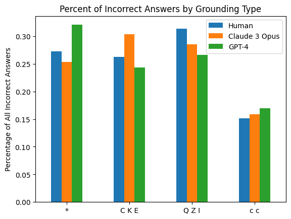| | Copy Context | Scrambled | Wrong Combination | Other | | --- | --- | --- | --- | --- | | Human | 0.192 | 0.020 | 0.556 | 0.232 | | GPT-4 | 0.239 | 0.031 | 0.502 | 0.228 | | Claude 3 Opus | 0.036 | 0.045 | 0.276 | 0.643 | <details> <summary>extracted/5679376/Images/incorrect_answers_by_grounding.png Details</summary>  ### Visual Description ## Bar Chart: Percent of Incorrect Answers by Grounding Type ### Overview The image is a grouped bar chart comparing the percentage of incorrect answers across four different "Grounding Types" for three distinct entities: Human, Claude 3 Opus, and GPT-4. The chart visually demonstrates how the error rate varies by grounding method and by the answering entity. ### Components/Axes * **Chart Title:** "Percent of Incorrect Answers by Grounding Type" * **Y-Axis:** * **Label:** "Percentage of All Incorrect Answers" * **Scale:** Linear scale from 0.00 to 0.30, with major tick marks at 0.05 intervals (0.00, 0.05, 0.10, 0.15, 0.20, 0.25, 0.30). * **X-Axis:** * **Categories (Grounding Types):** Four distinct categories are labeled: 1. `*` (asterisk) 2. `C K E` 3. `Q Z I` 4. `c c` * **Legend:** Located in the top-right corner of the plot area. It defines the three data series by color: * **Blue:** Human * **Orange:** Claude 3 Opus * **Green:** GPT-4 ### Detailed Analysis The chart presents the following approximate data points for each grounding type and entity. Values are estimated based on bar height relative to the y-axis grid. **1. Grounding Type: `*`** * **Human (Blue):** ~0.27 (27%) * **Claude 3 Opus (Orange):** ~0.25 (25%) * **GPT-4 (Green):** ~0.32 (32%) - This is the highest single value on the chart. **2. Grounding Type: `C K E`** * **Human (Blue):** ~0.26 (26%) * **Claude 3 Opus (Orange):** ~0.30 (30%) * **GPT-4 (Green):** ~0.24 (24%) **3. Grounding Type: `Q Z I`** * **Human (Blue):** ~0.31 (31%) * **Claude 3 Opus (Orange):** ~0.28 (28%) * **GPT-4 (Green):** ~0.26 (26%) **4. Grounding Type: `c c`** * **Human (Blue):** ~0.15 (15%) * **Claude 3 Opus (Orange):** ~0.16 (16%) * **GPT-4 (Green):** ~0.17 (17%) - This is the lowest set of values on the chart. ### Key Observations * **Highest Error Rate:** The single highest percentage of incorrect answers (~32%) is associated with **GPT-4** using the `*` grounding type. * **Lowest Error Rate:** The lowest error rates (~15-17%) are consistently found in the `c c` grounding type category for all three entities. * **Entity Performance Trends:** * **Human:** Shows the highest error rate in the `Q Z I` category (~31%) and the lowest in `c c` (~15%). * **Claude 3 Opus:** Peaks in the `C K E` category (~30%) and is lowest in `c c` (~16%). * **GPT-4:** Has its highest error rate in the `*` category (~32%) and its lowest in `c c` (~17%). * **Grounding Type Trends:** * The `c c` grounding type yields the most accurate results (lowest incorrect percentages) for all three entities. * The `*` and `Q Z I` grounding types are associated with higher error rates, though the specific entity that performs worst varies between them. ### Interpretation This chart suggests that the method of "grounding" (likely referring to how an AI or human is provided with context or evidence to answer a question) has a significant impact on accuracy. The `c c` grounding type appears to be the most effective for reducing errors across the board. The data also reveals that no single entity (Human, Claude 3 Opus, GPT-4) is universally the most accurate. Their relative performance is dependent on the grounding context: * GPT-4 is the least accurate with the `*` grounding. * Claude 3 Opus is the least accurate with the `C K E` grounding. * Humans are the least accurate with the `Q Z I` grounding. This implies that the interaction between the entity's capabilities and the specific grounding methodology is crucial. The chart does not explain what the grounding type labels (`*`, `C K E`, etc.) represent, but it clearly demonstrates that their design is a critical factor in performance outcomes. The notably low error rates for `c c` warrant further investigation into its methodology. </details> Figure 13: Percentage of incorrect answers in the Semantic Structure experiment by target domain type. In addition to the comparable mean performance, we find similar patterns in the errors made by humans and GPT-4. In Table 5 and Figure 13, one can see that the distribution of errors is comparable both when broken down by target domain type and when broken down by several error classifications we design. 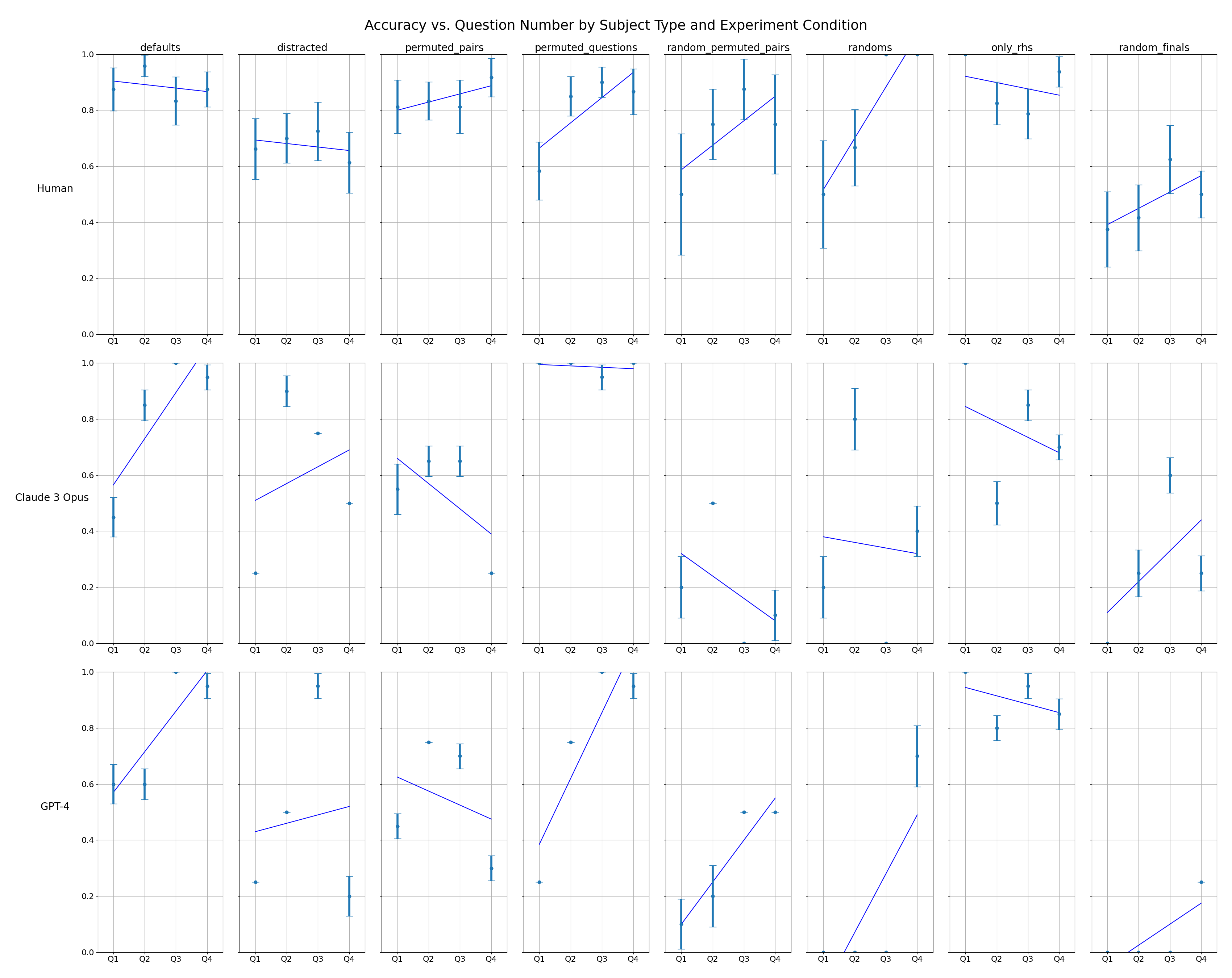<details> <summary>extracted/5679376/Images/top_performers_best_fit_and_points.png Details</summary>  ### Visual Description ## [Multi-Panel Line Chart]: Accuracy vs. Question Number by Subject Type and Experiment Condition ### Overview The image is a 3x8 grid of line charts (24 subplots total) displaying the accuracy of three different subjects (Human, Claude 3 Opus, GPT-4) across eight experimental conditions. Each subplot plots accuracy (y-axis) against question number (Q1, Q2, Q3, Q4) for a specific subject-condition pair. Blue lines connect the mean accuracy points, and vertical error bars indicate variability (likely standard deviation or confidence intervals). ### Components/Axes * **Overall Title:** "Accuracy vs. Question Number by Subject Type and Experiment Condition" * **Row Labels (Subject Type):** Located on the far left of each row. * Row 1: `Human` * Row 2: `Claude 3 Opus` * Row 3: `GPT-4` * **Column Headers (Experiment Condition):** Located at the top of each column. * Column 1: `defaults` * Column 2: `distracted` * Column 3: `permuted_pairs` * Column 4: `permuted_questions` * Column 5: `random_permuted_pairs` * Column 6: `randoms` * Column 7: `only_rhs` * Column 8: `random_finals` * **Axes (within each subplot):** * **Y-axis:** Label is implied by the overall title. Scale is from `0.0` to `1.0` (representing 0% to 100% accuracy). Major gridlines are at 0.0, 0.2, 0.4, 0.6, 0.8, 1.0. * **X-axis:** Discrete categories: `Q1`, `Q2`, `Q3`, `Q4`. * **Data Representation:** Blue line connecting data points with vertical error bars. ### Detailed Analysis **Row 1: Human** * **defaults:** Starts high (~0.9 at Q1), slight dip at Q2 (~0.85), stabilizes around 0.85-0.9 for Q3-Q4. Trend: Slight decline then stable. * **distracted:** Starts ~0.7 at Q1, declines steadily to ~0.6 at Q4. Trend: Downward. * **permuted_pairs:** Starts ~0.8 at Q1, rises to ~0.9 at Q4. Trend: Upward. * **permuted_questions:** Starts lower (~0.6 at Q1), rises sharply to ~0.9 at Q4. Trend: Strong upward. * **random_permuted_pairs:** Starts ~0.6 at Q1, rises to ~0.8 at Q4. Trend: Upward. * **randoms:** Starts low (~0.5 at Q1), rises sharply to 1.0 at Q4. Trend: Strong upward. * **only_rhs:** Starts high (~0.9 at Q1), declines slightly to ~0.85 at Q4. Trend: Slight downward. * **random_finals:** Starts low (~0.4 at Q1), rises to ~0.6 at Q4. Trend: Upward. **Row 2: Claude 3 Opus** * **defaults:** Starts low (~0.4 at Q1), rises steeply to 1.0 at Q4. Trend: Strong upward. * **distracted:** Starts very low (~0.25 at Q1), jumps to ~0.9 at Q2, then declines to ~0.5 at Q4. Trend: Sharp rise then decline. * **permuted_pairs:** Starts ~0.6 at Q1, declines to ~0.4 at Q4. Trend: Downward. * **permuted_questions:** Flat at 1.0 across all questions. Trend: Perfect and stable. * **random_permuted_pairs:** Starts ~0.3 at Q1, declines to ~0.1 at Q4. Trend: Downward. * **randoms:** Starts ~0.2 at Q1, rises to ~0.4 at Q4. Trend: Upward. * **only_rhs:** Starts ~0.85 at Q1, declines to ~0.7 at Q4. Trend: Downward. * **random_finals:** Starts ~0.1 at Q1, rises to ~0.4 at Q4. Trend: Upward. **Row 3: GPT-4** * **defaults:** Starts ~0.6 at Q1, rises to 1.0 at Q4. Trend: Upward. * **distracted:** Starts ~0.25 at Q1, rises to ~0.5 at Q4. Trend: Upward. * **permuted_pairs:** Starts ~0.45 at Q1, declines to ~0.3 at Q4. Trend: Downward. * **permuted_questions:** Starts ~0.25 at Q1, rises steeply to 1.0 at Q4. Trend: Strong upward. * **random_permuted_pairs:** Starts ~0.1 at Q1, rises to ~0.5 at Q4. Trend: Upward. * **randoms:** Starts at 0.0 at Q1, rises to ~0.5 at Q4. Trend: Strong upward. * **only_rhs:** Starts ~0.95 at Q1, declines to ~0.85 at Q4. Trend: Slight downward. * **random_finals:** Starts at 0.0 at Q1, rises to ~0.25 at Q4. Trend: Upward. ### Key Observations 1. **Performance Variability:** There is extreme variability in performance trends across subjects and conditions. No single pattern dominates. 2. **Human Consistency:** Human performance is generally more stable and less prone to extreme swings (e.g., from 0 to 1) compared to the AI models. 3. **AI Model Extremes:** Claude 3 Opus and GPT-4 show more dramatic performance shifts, including perfect scores (1.0) and near-zero scores (0.0) in certain conditions. 4. **Condition Impact:** The `permuted_questions` condition yields perfect accuracy for Claude 3 Opus but shows a strong learning curve for Humans and GPT-4. The `distracted` condition appears particularly harmful to initial performance for all subjects. 5. **Error Bars:** Error bars are generally larger for lower accuracy scores and for the AI models in challenging conditions, indicating higher uncertainty or variance in their responses. ### Interpretation This chart likely comes from a study comparing human and AI reasoning or problem-solving across a sequence of questions under different cognitive or structural manipulations. * **What the data suggests:** The experiment tests how performance evolves over a short sequence (Q1-Q4) when the problem format is altered (permuted, randomized, distracted). The stark differences between subjects suggest that humans and current large language models (Claude 3 Opus, GPT-4) employ fundamentally different strategies or have different vulnerabilities to these manipulations. * **How elements relate:** The grid structure allows direct comparison. For example, one can see that while Humans struggle with `distracted` (downward trend), GPT-4 shows improvement (upward trend), suggesting different attention mechanisms. The perfect flat line for Claude 3 Opus in `permuted_questions` indicates it may have a robust internal representation unaffected by question order, unlike Humans who must learn the pattern. * **Notable anomalies:** * Claude 3 Opus's `permuted_questions` performance is an outlier—perfect from the start. * GPT-4's `randoms` condition starts at 0.0 accuracy, suggesting complete failure on the first question, but shows rapid adaptation. * The `only_rhs` condition (possibly "only right-hand side" of an equation) shows a consistent slight downward trend for all subjects, implying it introduces a subtle but persistent difficulty. * **Underlying investigation:** The data probes the robustness and adaptability of reasoning systems. The trends help identify which types of problem transformations are most disruptive to different kinds of intelligence, informing both cognitive science and AI alignment research. The presence of learning curves (upward trends) versus degradation curves (downward trends) reveals whether a subject is adapting to the task structure or being confused by it. </details> Figure 14: Improvement in human and LLM accuracy by question number across different conditions. Error bars show standard errors. Further, humans and GPT-4 both improve as they see more questions over the course of a quiz. As seen in Figure 14, humans display a positive learning trend in 5 out of 8 conditions. GPT-4 displays a positive learning trend in a comparable 6 out of 8 conditions, with one of the conditions in which it does not display improvement resulting from it displaying near-perfect accuracy from start to finish (in the Only RHS condition). ### A.4 Further details of LLM performance Figure 15 shows the performance of all tested models in the Semantic Structure experiment. 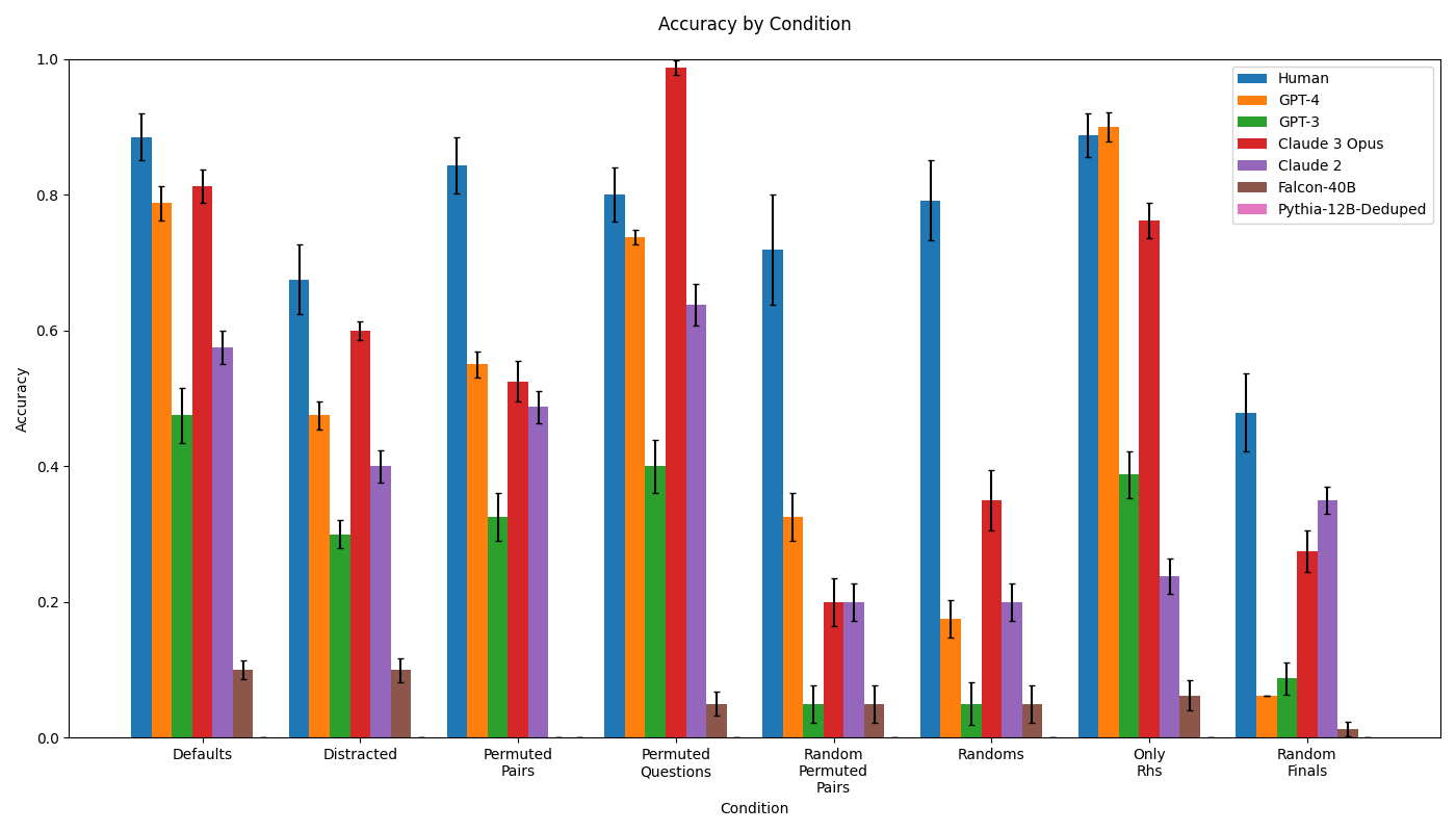<details> <summary>extracted/5679376/Images/Aggregate_Accuracy_Comparison.png Details</summary>  ### Visual Description ## Bar Chart: Accuracy by Condition ### Overview This is a grouped bar chart titled "Accuracy by Condition." It compares the performance accuracy of seven different entities (one human and six AI models) across eight distinct experimental conditions. The chart includes error bars for each data point, indicating variability or confidence intervals. The primary language is English. ### Components/Axes - **Title**: "Accuracy by Condition" (top center). - **Y-axis**: Labeled "Accuracy." Scale ranges from 0.0 to 1.0, with major tick marks at 0.0, 0.2, 0.4, 0.6, 0.8, and 1.0. - **X-axis**: Labeled "Condition." Contains eight categorical conditions: 1. Defaults 2. Distracted 3. Permuted Pairs 4. Permuted Questions 5. Random Permuted Pairs 6. Randoms 7. Only Rhs 8. Random Finals - **Legend**: Located in the top-right corner. Maps colors to entities: - Blue: Human - Orange: GPT-4 - Green: GPT-3 - Red: Claude 3 Opus - Purple: Claude 2 - Brown: Falcon-40B - Pink: Pythia-12B-Deduped - **Data Series**: Each condition on the x-axis has a cluster of up to seven bars, one for each entity in the legend. Error bars (black vertical lines) cap each bar. ### Detailed Analysis The following table reconstructs the approximate accuracy values for each entity across all conditions. Values are estimated from the bar heights relative to the y-axis. The presence of an error bar is noted, but its exact range is approximate. The entity "Pythia-12B-Deduped" (pink) does not have a visible bar in any condition, suggesting its accuracy is at or near 0.0 for all tests shown. | Condition | Human (Blue) | GPT-4 (Orange) | GPT-3 (Green) | Claude 3 Opus (Red) | Claude 2 (Purple) | Falcon-40B (Brown) | Pythia-12B-Deduped (Pink) | | :--- | :--- | :--- | :--- | :--- | :--- | :--- | :--- | | **Defaults** | ~0.88 (±0.04) | ~0.79 (±0.03) | ~0.48 (±0.04) | ~0.81 (±0.03) | ~0.58 (±0.03) | ~0.10 (±0.02) | Not visible (~0.0) | | **Distracted** | ~0.68 (±0.05) | ~0.48 (±0.02) | ~0.30 (±0.02) | ~0.60 (±0.02) | ~0.40 (±0.03) | ~0.10 (±0.02) | Not visible (~0.0) | | **Permuted Pairs** | ~0.84 (±0.05) | ~0.55 (±0.02) | ~0.33 (±0.04) | ~0.52 (±0.04) | ~0.49 (±0.03) | ~0.05 (±0.01) | Not visible (~0.0) | | **Permuted Questions** | ~0.80 (±0.04) | ~0.74 (±0.02) | ~0.40 (±0.04) | **~0.99 (±0.01)** | ~0.64 (±0.03) | ~0.05 (±0.02) | Not visible (~0.0) | | **Random Permuted Pairs** | ~0.72 (±0.08) | ~0.33 (±0.04) | ~0.05 (±0.03) | ~0.20 (±0.03) | ~0.20 (±0.03) | ~0.05 (±0.03) | Not visible (~0.0) | | **Randoms** | ~0.79 (±0.06) | ~0.18 (±0.03) | ~0.05 (±0.03) | ~0.35 (±0.05) | ~0.20 (±0.03) | ~0.05 (±0.03) | Not visible (~0.0) | | **Only Rhs** | ~0.89 (±0.03) | **~0.90 (±0.03)** | ~0.39 (±0.04) | ~0.76 (±0.03) | ~0.24 (±0.03) | ~0.06 (±0.03) | Not visible (~0.0) | | **Random Finals** | ~0.48 (±0.06) | ~0.06 (±0.03) | ~0.09 (±0.03) | ~0.28 (±0.03) | ~0.35 (±0.03) | ~0.01 (±0.01) | Not visible (~0.0) | ### Key Observations 1. **Human Performance**: Human accuracy (blue bars) is consistently high (≥0.68) across all conditions except "Random Finals," where it drops to ~0.48. It is the top or near-top performer in 6 of 8 conditions. 2. **Model Standouts**: - **Claude 3 Opus (Red)**: Achieves the single highest accuracy on the chart (~0.99) in the "Permuted Questions" condition. It is also strong in "Defaults" and "Only Rhs." - **GPT-4 (Orange)**: Matches or exceeds human performance in the "Only Rhs" condition (~0.90 vs ~0.89). It shows a significant performance drop in "Randoms" and "Random Finals." - **GPT-3 (Green) & Claude 2 (Purple)**: Show moderate performance, generally below GPT-4 and Claude 3 Opus. Claude 2 notably outperforms GPT-3 in most conditions. 3. **Low-Performing Models**: **Falcon-40B (Brown)** and **Pythia-12B-Deduped (Pink)** have very low accuracy across all conditions, with Falcon-40B peaking at ~0.10 and Pythia not registering a visible bar. 4. **Condition Difficulty**: The "Random Finals" condition appears to be the most challenging, causing the largest performance drop for the human and most models. Conversely, "Permuted Questions" and "Only Rhs" seem to be conditions where top models can excel. 5. **Error Bars**: The size of the error bars varies. Conditions like "Random Permuted Pairs" and "Randoms" show larger error bars for the human, suggesting greater variability in performance on those tasks. ### Interpretation This chart likely presents results from a benchmarking study evaluating reasoning or knowledge recall under different data presentation or perturbation conditions. The conditions ("Permuted Pairs," "Random Finals," etc.) suggest tests of robustness to scrambled inputs, distractors, or altered question formats. The data demonstrates a clear performance hierarchy: **Human ≈ Claude 3 Opus ≈ GPT-4 > Claude 2 > GPT-3 >> Falcon-40B ≈ Pythia-12B-Deduped**. The exceptional performance of Claude 3 Opus on "Permuted Questions" indicates a specific strength in that type of reasoning task. The fact that GPT-4 matches human performance on "Only Rhs" (possibly "Only Right-hand Sides" of an equation or analogy) suggests it has mastered that particular sub-task. The dramatic drop in accuracy for all entities on "Random Finals" implies this condition removes a critical structural cue or introduces noise that severely disrupts the reasoning process. The near-zero performance of the smaller models (Falcon-40B, Pythia-12B-Deduped) across the board highlights a significant capability gap between larger, more advanced models and smaller ones on these specific tasks. The chart effectively communicates that model size and architecture (as represented by the different model names) are strong predictors of performance on this benchmark, with human-level performance being attainable by the top models under certain conditions. </details> Figure 15: Performance of all tested models in the Semantic Structure experiment. Error bars show standard errors. Figure 16 shows the variation in the performance of GPT-4 in two conditions (Only RHS and Random Finals) across various small differences in prompting strategy. With small differences in prompting strategy, performance in the Only RHS condition varies between approximately 20% and approximately 100%. Similarly, small differences in the prompting strategy yield performance in the Random Finals condition that varies between near-zero and close to 40%. Such variation is very significant, but appears in general to be fairly explicable. In the Only RHS condition, the majority of the variation appears to come from setting up the prompt in such a way that it is clear that a final term is desired next, as opposed to a new question. In the other conditions, an arrow separator that divides left- and right-hand side terms is the final element of the prompt, thus suggesting that a right-hand term is appropriate as the next token. In the Only RHS condition, this trailing separator was initially not present, and thus the models often responded by beginning a new question rather than by completing the last question presented. Re-introducing arrow separators and making other small changes designed to more clearly indicate when a question has not yet been completed eliminates these kinds of errors and drastically increases performance. In the Random Finals condition, a significant improvement comes from changing the instruction sentence from one that specifies that a drawing of the left-hand side is requested, to an instruction sentence specifying that various patterns will be shown after which the last should be completed. This is reasonable, as in this condition the final left-hand term is misleading and so an instruction focusing attention on it is expected to reduce performance. As expected, no performance improvement is observed when replacing the set of random final words with different ones. Finally, a performance boost is observed when adding additional newlines (instead of only having a clear line between each question, we now also include a clear line between each line of a question). It is not clear why this should improve performance. 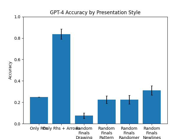<details> <summary>extracted/5679376/Images/gpt4_tweak_dependance.png Details</summary>  ### Visual Description ## Bar Chart: GPT-4 Accuracy by Presentation Style ### Overview This is a vertical bar chart titled "GPT-4 Accuracy by Presentation Style." It compares the accuracy of the GPT-4 model across six different presentation styles or conditions. The chart includes error bars for each data point, indicating variability or confidence intervals. The overall visual trend shows one condition ("Only Rhs + Arrow") performing significantly better than all others. ### Components/Axes * **Title:** "GPT-4 Accuracy by Presentation Style" (centered at the top). * **Y-Axis:** * **Label:** "Accuracy" (rotated vertically on the left side). * **Scale:** Linear scale from 0.0 to 1.0, with major tick marks at 0.0, 0.2, 0.4, 0.6, 0.8, and 1.0. * **X-Axis:** * **Categories (from left to right):** 1. "Only Rhs" 2. "Only Rhs + Arrow" 3. "Random Finals Drawing" 4. "Random Finals Pattern" 5. "Random Finals Randomer" 6. "Random Finals Newlines" * **Data Series:** A single series represented by blue bars. Each bar has a black error bar (whisker) extending above and below the top of the bar. * **Legend:** No separate legend is present; the categories are labeled directly on the x-axis. ### Detailed Analysis The following table reconstructs the approximate data from the chart. Values are estimated based on the bar heights relative to the y-axis grid. | Presentation Style | Approximate Accuracy | Error Bar Range (Visual Estimate) | Trend Description | | :--- | :--- | :--- | :--- | | **Only Rhs** | ~0.25 | Very small range, approximately ±0.01 | A short bar, indicating low accuracy. | | **Only Rhs + Arrow** | ~0.83 | Moderate range, approximately ±0.05 (from ~0.78 to ~0.88) | The tallest bar by a large margin, showing high accuracy. | | **Random Finals Drawing** | ~0.08 | Moderate range, approximately ±0.03 (from ~0.05 to ~0.11) | The shortest bar, indicating the lowest accuracy. | | **Random Finals Pattern** | ~0.22 | Moderate range, approximately ±0.04 (from ~0.18 to ~0.26) | Similar in height to "Only Rhs" and "Random Finals Randomer". | | **Random Finals Randomer** | ~0.22 | Moderate range, approximately ±0.04 (from ~0.18 to ~0.26) | Nearly identical in height and error to "Random Finals Pattern". | | **Random Finals Newlines** | ~0.31 | Moderate range, approximately ±0.05 (from ~0.26 to ~0.36) | Slightly taller than the previous two "Random Finals" variants. | ### Key Observations 1. **Dominant Performance:** The "Only Rhs + Arrow" condition is a clear outlier, achieving an accuracy (~0.83) more than three times higher than the next best condition. 2. **Low Baseline:** The "Only Rhs" condition (without an arrow) has a low accuracy (~0.25), suggesting the arrow is a critical component for the high performance in the second condition. 3. **Poor Performance of Randomization:** All conditions labeled "Random Finals..." perform poorly, with accuracies between ~0.08 and ~0.31. The "Drawing" variant is particularly ineffective. 4. **Clustering of Results:** The accuracies for "Only Rhs," "Random Finals Pattern," and "Random Finals Randomer" are all clustered in a similar low range (~0.22-0.25). 5. **Error Bars:** The error bars are relatively small for the lowest-performing condition ("Random Finals Drawing") and largest for the highest-performing one ("Only Rhs + Arrow"), which may indicate greater variance in results when accuracy is high. ### Interpretation The data strongly suggests that the **presentation style has a dramatic impact on GPT-4's accuracy** for the given task. The key finding is the synergistic effect of combining "Only Rhs" with an "Arrow." This specific visual or structural cue appears to be a highly effective scaffold for the model, leading to a massive performance boost. Conversely, introducing randomness into the "Finals" (likely meaning the final part of a prompt or output) through various methods ("Drawing," "Pattern," "Randomer," "Newlines") consistently degrades performance compared to the structured "Only Rhs + Arrow" condition. This implies that predictability and clear visual guidance are more beneficial than varied or unstructured presentations for this particular evaluation. The chart demonstrates that minor changes in prompt or output formatting (like adding an arrow) can lead to order-of-magnitude differences in model performance, highlighting the importance of prompt engineering and the sensitivity of large language models to input structure. </details> Figure 16: Dependence of GPT-4 accuracy on prompt variations. Error bars show standard errors. | Prompt | We are conducting an experiment on general reasoning abilities. Below we will show you various words and drawings of each, after which you will need to complete the last drawing. Respond as concisely as possible with only the last drawing. Question 1: chicken => ! spider => ! cat => * horse => * ant => ! dog => * bee => ! human => * Question 2: car => * tricycle => ! motorcycle => * skateboard => ! bicycle => ! unicycle => ——— SAMPLED RESPONSE SET ——— ! [Continuation omitted] —————————————- ! [Continuation omitted] —————————————- * [Continuation omitted] —————————————- ! [Continuation omitted] —————————————- * [Continuation omitted] | | --- | --- | Table 6: Table showing an illustrative response from Falcon-40B in the Categorial condition of the Semantic Content experiment. Observe that the model provides incorrect and correct responses to the question, seeming to recognize the form of a correct response but to not reason further about correctness. | Prompt | We are conducting an experiment on general reasoning abilities. Below we will show you various words and drawings of each, after which you will need to complete the last drawing. Respond as concisely as possible with only the last drawing. Question 1: spider => * * * * * * * * human => * * cat => * * * * chicken => * * dog => * * * * horse => * * * * bee => * * * * * * Question 2: motorcycle => * * tricycle => * * * bicycle => * * unicycle => * car => ——— SAMPLED RESPONSE SET ——— * * * —————————————- * * —————————————- * * —————————————- * * —————————————- * * | | --- | --- | Table 7: Table showing an illustrative response from GPT-4 in the numerical condition of the Semantic Content experiment. Observe that the model fails to correctly relate the number of characters to the numerical property of the object, in this case the number of wheels that a car has. | Prompt | * * * + * = * * * * * * * * * – * * = * * * * * * * * * – * * * = | | --- | --- | | Responses | * * * * * * (first response) * * * * * * (second response) * * * * * * * (third response) | | Expected result | * * * | Table 8: Table showing a sanity check that GPT-4 fails to reason about the number of characters in the expected way. Settings: temperature 1, maximum length 256, top P 1.